Compound Poisson disorder problem Savas Dayanik Princeton University, Department of Operations Research and Financial Engineering, and Bendheim Center for Finance, Princeton, NJ 08544 email: [email protected] http://www.princeton.edu/ ∼ sdayanik Semih Onur Sezer Princeton University, Department of Operations Research and Financial Engineering, Princeton, NJ 08544 email: [email protected] http://www.princeton.edu/ ∼ ssezer This paper is dedicated to our teacher and mentor, Professor Erhan C ¸ınlar, on the occasion of his 65th birthday. In compound Poisson disorder problem, arrival rate and/or jump distribution of some compound Poisson process change suddenly at some unknown and unobservable time. The problem is to detect the change (or disorder) time as quickly as possible. A sudden regime-shift may require some counter-measures be taken promptly, and a quickest detection rule can help with those efforts. We describe complete solution of compound Poisson disorder problem with several standard Bayesian risk measures. Solution methods are feasible for numerical implementation and are illustrated on examples. Key words: Poisson disorder problem; quickest detection; compound Poisson processes, optimal stopping MSC2000 Subject Classification: Primary: 62L10; Secondary: 62L15, 62C10, 60G40 OR/MS subject classification: Primary: Statistics: Bayesian, Estimation; Secondary: Dynamic program- ming/optimal control: Applications 1. Introduction. Let (Ω, F, P) be a probability space hosting a compound Poisson process X t = X 0 + Nt k=1 Y k , t ≥ 0. (1) Jumps arrive according to a standard Poisson process N = {N t ; t ≥ 0} at some rate λ 0 > 0. The marks at each jump are i.i.d. R d -valued random variables Y 1 ,Y 2 ,... with some common distribution ν 0 (·) independent of the arrival process N . The process X may represent customer orders arriving in batches to a multi-product service system, claims of various sizes filed with an insurance company, or sizes of electronic files requested for download from a network server. Suppose that, at an unknown and unobservable time θ, the initial arrival rate λ 0 and mark distribution ν 0 (·) of the process X change suddenly to λ 1 and ν 1 (·), respectively. This regime shift at the disorder time θ may become detrimental on the underlying system unless certain counter-measures are taken quickly. For example, optimal inventory levels, insurance premiums, or number of network servers may need to be revised as soon as the regime changes in order to maintain profitability, avoid bankruptcy, or ensure the network availability. The objective of this paper is to detect the disorder time θ as quickly as possible in order to give decision makers an opportunity to react the regime change on a timely basis. We assume that λ 0 , λ 1 , ν 0 (·) and ν 1 (·) are known, and that the disorder time θ is a random variable whose prior distribution is P{θ =0} = π and P{θ>t} = (1 - π)e -λt , t ≥ 0; π ∈ [0, 1),λ> 0. The disorder time θ is still unobservable, and we need a quickest detection rule adapted to the history F of the observation process X in (1). More precisely, we would like to find a stopping time τ of the process X whose Bayes risk R τ (π) P{τ<θ} + c E(τ - θ) + , π ∈ [0, 1),τ ∈ F (2) is the smallest (x + max{x, 0}.) If an F-stopping time τ attains the minimum Bayes risk U (π) inf τ ∈F R τ (π), π ∈ [0, 1), (3) then it is called a Bayes-optimal alarm time and solves optimally the tradeoff between the false-alarm frequency P{τ<θ} and the expected detection delay cost c · E(τ - θ) + . 1

Welcome message from author
This document is posted to help you gain knowledge. Please leave a comment to let me know what you think about it! Share it to your friends and learn new things together.
Transcript

Compound Poisson disorder problem
Savas DayanikPrinceton University, Department of Operations Research and Financial Engineering, and Bendheim Center for
Finance, Princeton, NJ 08544
email: [email protected] http://www.princeton.edu/∼sdayanik
Semih Onur SezerPrinceton University, Department of Operations Research and Financial Engineering, Princeton, NJ 08544
email: [email protected] http://www.princeton.edu/∼ssezer
This paper is dedicated to our teacher and mentor,Professor Erhan Cınlar, on the occasion of his 65th birthday.
In compound Poisson disorder problem, arrival rate and/or jump distribution of some compound Poisson processchange suddenly at some unknown and unobservable time. The problem is to detect the change (or disorder)time as quickly as possible. A sudden regime-shift may require some counter-measures be taken promptly, and aquickest detection rule can help with those efforts. We describe complete solution of compound Poisson disorderproblem with several standard Bayesian risk measures. Solution methods are feasible for numerical implementationand are illustrated on examples.
Key words: Poisson disorder problem; quickest detection; compound Poisson processes, optimal stopping
MSC2000 Subject Classification: Primary: 62L10; Secondary: 62L15, 62C10, 60G40
OR/MS subject classification: Primary: Statistics: Bayesian, Estimation; Secondary: Dynamic program-ming/optimal control: Applications
1. Introduction. Let (Ω,F, P) be a probability space hosting a compound Poisson process
Xt = X0 +Nt∑
k=1
Yk, t ≥ 0. (1)
Jumps arrive according to a standard Poisson process N = Nt; t ≥ 0 at some rate λ0 > 0. Themarks at each jump are i.i.d. Rd-valued random variables Y1, Y2, . . . with some common distribution ν0(·)independent of the arrival process N . The process X may represent customer orders arriving in batchesto a multi-product service system, claims of various sizes filed with an insurance company, or sizes ofelectronic files requested for download from a network server.
Suppose that, at an unknown and unobservable time θ, the initial arrival rate λ0 and mark distributionν0(·) of the process X change suddenly to λ1 and ν1(·), respectively. This regime shift at the disorder timeθ may become detrimental on the underlying system unless certain counter-measures are taken quickly.For example, optimal inventory levels, insurance premiums, or number of network servers may need tobe revised as soon as the regime changes in order to maintain profitability, avoid bankruptcy, or ensurethe network availability.
The objective of this paper is to detect the disorder time θ as quickly as possible in order to givedecision makers an opportunity to react the regime change on a timely basis. We assume that λ0, λ1,ν0(·) and ν1(·) are known, and that the disorder time θ is a random variable whose prior distribution is
Pθ = 0 = π and Pθ > t = (1− π)e−λt, t ≥ 0; π ∈ [0, 1), λ > 0.
The disorder time θ is still unobservable, and we need a quickest detection rule adapted to the history Fof the observation process X in (1). More precisely, we would like to find a stopping time τ of the processX whose Bayes risk
Rτ (π) , Pτ < θ+ c E(τ − θ)+, π ∈ [0, 1), τ ∈ F (2)
is the smallest (x+ , maxx, 0.) If an F-stopping time τ attains the minimum Bayes risk
U(π) , infτ∈F
Rτ (π), π ∈ [0, 1), (3)
then it is called a Bayes-optimal alarm time and solves optimally the tradeoff between the false-alarmfrequency Pτ < θ and the expected detection delay cost c · E(τ − θ)+.
1
2 S. Dayanik and S. O. Sezer: Compound Poisson disorder problemMathematics of Operations Research xx(x), pp. xxx–xxx, c©200x INFORMS
All of the early work has dealed with (simple) Poisson disorder problem. In that problem and inthe notation above, the observation process was the counting process N whose rate changes at someunobservable time θ from some known constant λ0 to some other λ1. While the question was the same;namely, to detect the disorder time θ as quickly as possible, the information about marks Y1, Y2, . . . wereignored completely. This omission was understandable because of the difficulty of the problem: simplePoisson disorder problem was solved completely by Peskir and Shiryaev [13] only recently—more thanthirty years after it was formulated by Galchuk and Rozovskii [9] for the first time. In the meantime,partial solutions and new insights were provided. Most notably, Davis [5] showed that quickest detectionrules should not differ much if they are to minimize some “standard” Bayes risks; namely, one of R(1),R(2) (same as R of (2)), or R(3) in
R(1)τ (π) , Pτ < θ − ε+ c E(τ − θ)+, R(2)
τ (π) , Pτ < θ+ c E(τ − θ)+,
R(3)τ (π) , E(θ − τ)+ + c E(τ − θ)+, R(4)
τ (π) , Pτ < θ+ c E[eα(τ−θ)+ − 1],(4)
where ε, c, and α are some known positive constants (see also Shiryaev [17]). Recently, Bayraktarand Dayanik [1] solved simple Poisson disorder problem with Bayes risk R(4) in (4), whose exponentialdetection-delay penalty makes it more suitable for financial applications. Later, Bayraktar, Dayanik,and Karatzas [2] showed that the measure R(4) is also a “standard” Bayes risk (if the latter is redefinedsuitably) and gave a general solution method for standard problems.
For the first time, Gapeev [10] has recently succeeded to include the observed marks Y1, Y2, . . . into anoptimal decision rule in order to detect the disorder time (more) quickly and accurately. He provided thefull solution for the following very special instance of compound Poisson disorder problem: before andafter the disorder time θ, real-valued marks Y1, Y2, . . . have exponential distributions, and the expectedmark sizes are the same as the corresponding jump arrival rates. Namely, the mark distributions are
νi(A) =∫
A
1λi
exp− 1
λiy
dy, A ∈ B(R+), i = 0, 1, (5)
where λ0 and λ1 are the arrival rates of jumps (i.e., the counting process N in (1)) before and after thedisorder, respectively.
The main contribution of our paper is the complete solution of compound Poisson disorder problemin its full generality. For any pair of arrival rates λ0 and λ1 and mark distributions ν0(·) and ν1(·), wedescribe explicitly a quickest detection rule. These rules depend on the some F-adapted odds-ratio processΦ = Φt; t ≥ 0; see (11). At every t ≥ 0, the random variable Φt is the conditional odds-ratio of theevent θ ≤ t that disorder has happened at or before time t given past and present observations Ft ofthe process X. For a suitable constant ξ > 0, the first crossing time U0 = inft ≥ 0 : Φt ≥ ξ of theprocess Φ turns out to be a quickest detection rule: the Bayes risk RU0 in (2) of U0 is the smallest amongall of the stopping times of the process X. The critical threshold ξ can be calculated numerically, andthe quickest detection rule U0 is suitable for online implementation since Φt, t ≥ 0 can be updated by arecursive formula; see (13).
We also show that every compound Poisson disorder problem with one of “standard” Bayes risks in(4) can be solved in the same way.
Our probabilistic methods are different from the analytical methods of all previously cited work. Thelatter attacked Poisson disorder problems by studying analytical properties of related free-boundaryintegro-differential equations. Instead, we study very carefully sample-paths of the process Φ, which turnout to be piecewise deterministic and Markovian. General characterization of stopping times of jumpprocesses allows us to approximate the minimum Bayes risk successively. This approximation is the keyto our computational and theoretical results.
In the next section we give the precise description of compound Poisson disorder problem and showhow to reduce it to an optimal stopping problem for a suitable Markov process. In Sections 3 and 4, weintroduce successive approximations of the value function of the optimal stopping problem and establishkey results for an efficient numerical method, which is presented in Section 5. We illustrate this methodon several old and new examples and discuss briefly some extensions in Section 6. Finally, we establishin Section 7 the connection between our method and method of variational inequalities as applied tocompound Poisson disorder problem. Appendix A contains some basic derivations and long proofs.

S. Dayanik and S. O. Sezer: Compound Poisson disorder problemMathematics of Operations Research xx(x), pp. xxx–xxx, c©200x INFORMS 3
2. Model and problem description. Starting with a reference probability measure, we shall firstconstruct a model containing all of the random elements of our problem with the correct probability laws.
Model. Let (Ω,F, P0) be a probability space hosting the following independent stochastic elements:
(i) a standard Poisson process N = Nt; t ≥ 0 with the arrival rate λ0,
(ii) independent and identically distributed Rd-valued random variables Y1, Y2, . . . with some commondistribution ν0(B) , P0Y1 ∈ B for every set B in the Borel σ-algebra B(Rd) and ν0(0) = 0,
(iii) a random variable θ with the distribution
P0θ = 0 = π ∈ [0, 1) and P0θ > t = (1− π)e−λt, t ≥ 0, λ > 0. (6)
Let X = Xt; t ≥ 0 be the process defined by (1) with the jump times
σn , inft > σn−1 : Xt 6= Xt−, n ≥ 1 (σ0 ≡ 0), (7)
and F = Ftt≥0 be the augmentation of its natural filtration σ(Xs, s ≤ t), t ≥ 0 with P0-null sets. Thenthe process X is a (P0, F)-compound Poisson process with the arrival rate λ0 and the jump distributionν0(·).
Let λ1 > 0 be a constant, and ν1(·) be a probability measure on (Rd,B(Rd)) absolutely continuous withrespect to the distribution ν0(·). In general, every probability measure ν1(·) is the sum of two probabilitymeasures; one is singular, and the other is absolutely continuous with respect to ν0(·). If it is necessary,the distribution ν1(·) is replaced with its component which is absolutely continuous with respect to themeasure ν0(·) without loss of generality as explained by Poor [14, pp. 269-271]. Then the Radon-Nikodymderivative
f(y) ,dν1
dν0
∣∣∣∣B(Rd)
(y), y ∈ Rd (8)
of ν1(·) with respect to ν0(·) exists and is a ν0-a.e. nonnegative Borel function.
We shall denote by G = Gtt≥0 and Gt , Ft ∨σ(θ), t ≥ 0 the enlargement of the filtration F with thesigma-algebra σ(θ) generated by θ. Let us define a new probability measure P on the measurable space(Ω,∨s≥0Gs) locally in terms of the Radon-Nikodym derivatives
dPdP0
∣∣∣∣Gt
= Zt , 1t<θ + 1t≥θe−(λ1−λ0)(t−θ)
Nt∏k=Nθ−+1
[λ1
λ0f(Yk)
], t ≥ 0, (9)
where Nθ− is the number of arrivals in the time-interval [0, θ). If the disorder time θ is known, then eachrandom variable Zt is simply the likelihood ratio of the interarrival times σ1, σ2−σ1, . . . and the jump sizesY1, Y2, . . . observed at or before time t. Under P, the interarrival times and jump sizes are conditionallyindependent and have the desired conditional distributions given θ: the rate of exponentially distributedinterarrival times and the distribution of the jump sizes change at time θ from λ0 and ν0(·) to λ1 andν1(·), respectively. See also Appendix A.1 for another justification by using an absolutely continuouschange of measure for point processes.
Finally, because Z0 = 1 almost surely and the probability measures P0 and P coincide on G0 = σ(θ),the distribution of θ is the same under P and P0. Hence, under the probability measure P defined by(9), the process X and the random variable θ have the same properties as in the setup of the disorderproblem described in the introduction.
Problem description. In the remainder, we shall work with the concrete model described above.The random variable θ is the unobservable disorder time and must be detected as quickly as possible asthe history F of the observation process X is unfolded. The admissible detection rules are the stoppingtimes of the filtration F.
Our problem is to find the smallest Bayes risk U(·) in (3) by minimizing over all stopping rules τ of thefiltration F the tradeoff Rτ (·) in (2) between the false-alarm frequency and expected detection delay cost.If this infimum is attained, then we also want to describe explicitly a stopping rule with the minimumBayes risk.

4 S. Dayanik and S. O. Sezer: Compound Poisson disorder problemMathematics of Operations Research xx(x), pp. xxx–xxx, c©200x INFORMS
In the remainder of this section, we shall formulate the quickest-detection problem as an optimalstopping problem for a suitable Markov process; see (16) below. In later sections, we solve this optimalstopping problem completely and identify an optimal stopping rule.
One may check as in Bayraktar, Dayanik, and Karatzas [2, Proposition 2.1] that the Bayes risk in (2)can be expressed as
Rτ (π) = (1− π) + c(1− π) E0
[∫ τ
0
e−λt
(Φt −
λ
c
)dt
], π ∈ [0, 1), τ ∈ F (10)
in terms of the F-adapted odds-ratio process
Φt ,Pθ ≤ t|FtPθ > t|Ft
, t ≥ 0. (11)
For every t ≥ 0, the random variable Φt is the conditional odds-ratio of the event that the disorderhappened at or before time t given the history Ft of the process X. In (10), the expectation E0 is takenwith respect to P0, and the probability measure P in (11) is defined by the absolutely continuous changeof measure in (9).
In Appendix A.2, we show that the process Φ = Φt; t ≥ 0 in (11) is a piecewise-deterministic Markovprocess (Davis [6, 7]). If we define
a , λ− λ1 + λ0, φd ,
− λ/a, if a 6= 0−∞, if a = 0
,
x(t, φ) ,
φd + eat [φ− φd] , a 6= 0φ + λt, a = 0
, t ∈ R, φ ∈ R.
(12)
and the σn, n ≥ 0 are the jump times in (7) of the process X, then we getΦt = x
(t− σn−1,Φσn−1
), t ∈ [σn−1, σn)
Φσn=
λ1
λ0f(Yn)Φσn−
, n ≥ 1. (13)
Namely, the process Φ follows one of the deterministic curves t 7→ x(t, φ), φ ∈ R in (12) betweenconsecutive jumps of X and is updated instantaneously at every jump of X as in (13); see also Figure 1on page 9. The (P0, F)-infinitesimal generator of the process Φ coincides on the collection of continuouslydifferentiable functions h : R+ 7→ R with the first-order integro-differential operator (see Appendix A.3)
Ah(x) = [λ + ax]h′(x) + λ0
∫y∈Rd
[h
(λ1
λ0f(y) x
)− h(x)
]ν0(dy), x ∈ R+. (14)
Finally, the minimum Bayes risk in (3, 10) is given by
U(π) = (1− π) + c(1− π) V
(π
1− π
), π ∈ [0, 1) (15)
in terms of the value function
V (φ) , infτ∈F
Eφ0
[∫ τ
0
e−λtg(Φt)dt
], φ ∈ R+ (16)
of a discounted optimal stopping problem with the running cost
g(φ) , φ− λ
c, φ ∈ R+ (17)
and discount rate λ > 0 for the piecewise-deterministic Markov process Φ in (13). In (16), the expectationEφ
0 is taken with respect to the probability measure P0 and P0Φ0 = φ = 1.
Thus, our problem becomes to calculate the value function V (·) in (16) and to find an optimal stoppingrule if the infimum is attained. Our approach is direct and very suitable for piecewise-deterministicMarkov processes. The solution is described in Section 5 in terms of single-jump operators after keyresults are established in Sections 3 and 4.
S. Dayanik and S. O. Sezer: Compound Poisson disorder problemMathematics of Operations Research xx(x), pp. xxx–xxx, c©200x INFORMS 5
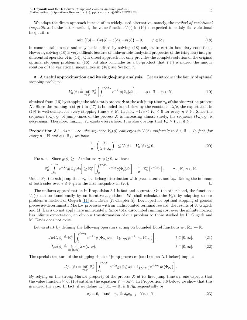
We adopt the direct approach instead of its widely-used alternative, namely, the method of variationalinequalities. In the latter method, the value function V (·) in (16) is expected to satisfy the variationalinequalities
min (A− λ)v(φ) + g(φ),−v(φ) = 0, φ ∈ R+ (18)
in some suitable sense and may be identified by solving (18) subject to certain boundary conditions.However, solving (18) is very difficult because of unfavorable analytical properties of the (singular) integro-differential operator A in (14). Our direct approach not only provides the complete solution of the originaloptimal stopping problem in (16), but also concludes as a by-product that V (·) is indeed the uniquesolution of the variational inequalities in (18); see Section 7.
3. A useful approximation and its single-jump analysis. Let us introduce the family of optimalstopping problems
Vn(φ) , infτ∈F
Eφ0
[∫ τ∧σn
0
e−λtg(Φt)dt
], φ ∈ R+, n ∈ N, (19)
obtained from (16) by stopping the odds-ratio process Φ at the nth jump time σn of the observation processX. Since the running cost g(·) in (17) is bounded from below by the constant −λ/c, the expectation in(19) is well-defined for every stopping time τ ∈ F. In fact, −1/c ≤ Vn ≤ 0 for every n ∈ N. Since thesequence (σn)n≥1 of jump times of the process X is increasing almost surely, the sequence (Vn)n≥1 isdecreasing. Therefore, limn→∞ Vn exists everywhere. It is also obvious that Vn ≥ V , n ∈ N.
Proposition 3.1 As n → ∞, the sequence Vn(φ) converges to V (φ) uniformly in φ ∈ R+. In fact, forevery n ∈ N and φ ∈ R+, we have
−1c·(
λ0
λ + λ0
)n
≤ V (φ)− Vn(φ) ≤ 0. (20)
Proof. Since g(φ) ≥ −λ/c for every φ ≥ 0, we have
Eφ0
[∫ τ
0
e−λsg(Φs)ds
]≥ Eφ
0
[∫ τ∧σn
0
e−λsg(Φs)ds
]− 1
c· Eφ
0
[e−λσn
], τ ∈ F, n ∈ N.
Under P0, the nth jump time σn has Erlang distribution with parameters n and λ0. Taking the infimumof both sides over τ ∈ F gives the first inequality in (20).
The uniform approximation in Proposition 3.1 is fast and accurate. On the other hand, the functionsVn(·) can be found easily by an iterative algorithm. We shall calculate the Vn’s by adapting to ourproblem a method of Gugerli [11] and Davis [7, Chapter 5]. Developed for optimal stopping of generalpiecewise-deterministic Markov processes with an undiscounted terminal reward, the results of U. Gugerliand M. Davis do not apply here immediately. Since total discounted running cost over the infinite horizonhas infinite expectation, an obvious transformation of our problem to those studied by U. Gugerli andM. Davis does not exist.
Let us start by defining the following operators acting on bounded Borel functions w : R+ 7→ R:
Jw(t, φ) , Eφ0
[∫ t∧σ1
0
e−λug (Φu) du + 1t≥σ1e−λσ1w (Φσ1)
], t ∈ [0,∞], (21)
Jtw(φ) , infu∈[t,∞]
Jw(u, φ), t ∈ [0,∞]. (22)
The special structure of the stopping times of jump processes (see Lemma A.1 below) implies
J0w(φ) = infτ∈F
Eφ0
[∫ τ∧σ1
0
e−λtg (Φt) dt + 1τ≥σ1e−λσ1w (Φσ1)
].
By relying on the strong Markov property of the process X at its first jump time σ1, one expects thatthe value function V of (16) satisfies the equation V = J0V . In Proposition 3.6 below, we show that thisis indeed the case. In fact, if we define vn : R+ 7→ R, n ∈ N0, sequentially by
v0 ≡ 0, and vn , J0vn−1 ∀n ∈ N, (23)
6 S. Dayanik and S. O. Sezer: Compound Poisson disorder problemMathematics of Operations Research xx(x), pp. xxx–xxx, c©200x INFORMS
then every vn is bounded and identical to Vn of (19), limn→∞ vn exists and equals the value function Vin (16); see Corollary 3.4 and Proposition 3.5.
Under P0, the first jump time σ1 of the process X has exponential distribution with rate λ0. Usingthe Fubini theorem and (13), we can write (21) as
Jw(t, φ) =∫ t
0
e−(λ+λ0)u(g + λ0 · Sw
)(x(u, φ)
)du, t ∈ [0,∞], (24)
where the function x(·, φ) is given by (12), and S is the linear operator
Sw(x) ,∫
Rd
w
(λ1
λ0f(y) x
)ν0(dy), x ∈ R, (25)
defined on the collection of bounded functions w : R 7→ R.
Remark 3.2 Using the explicit form of x(u, φ) in (12), it is easy to check that the integrand in (24) isabsolutely integrable on R+. Therefore,
limt→∞
Jw(t, φ) = Jw(∞, φ) < ∞,
and the mapping t 7→ Jw(t, φ) : [0,+∞] 7→ R is continuous. Therefore, the infimum Jtw(φ) in (22) isattained for every t ∈ [0,∞].
Lemma 3.3 For every bounded Borel function w : R+ 7→ R, the mapping J0w is bounded. If we define||w|| , supφ∈R+
|w(φ)| < ∞, then
−(
λ
λ + λ0· 1c
+λ0
λ + λ0· ||w||
)≤ J0w(φ) ≤ 0, φ ∈ R+. (26)
If the function w(·) is concave, then so is J0w(·). If w1(·) ≤ w2(·) are real-valued and bounded Borelfunctions defined on R+, then J0w1(·) ≤ J0w2(·). Namely, the operator J0 preserves the boundedness,concavity, and monotonicity.
Proof. The lower bound in (26) follows from the lower bound −λ/c on the running cost g(·) in (16).The concavity and the monotonicity can be checked directly.
Corollary 3.4 Every vn, n ∈ N0 in (23) is bounded and concave, and −1/c ≤ . . . ≤ vn ≤ vn−1 ≤ v1 ≤v0 ≡ 0. The limit
v(φ) , limn→∞
vn(φ), φ ∈ R+ (27)
exists, and is bounded, concave, and nondecreasing. Both vn : R+ 7→ R, n ∈ N and v : R+ 7→ R arecontinuous and nondecreasing. Their left and right derivatives are bounded on every compact subset ofR+.
Proof. By definition, v0 ≡ 0 is bounded, concave, and nondecreasing. By an induction argumenton n, the conclusions follow from Lemma 3.3, the properties of concave functions, and the monotonicityof the functions x(t, ·) for every fixed t ∈ R and g(·) in (12) and (17), and the operator S in (25).
Next proposition describes some ε-optimal stopping rules for each problem in (19). In conjunctionwith Proposition 3.6 below, it is the basic block of the numerical scheme described in Section 5. Its proofis presented in Section A.4.
Proposition 3.5 For every n ∈ N, the functions vn of (23) and Vn of (19) coincide. For every ε ≥ 0,let
rεn(φ) , inf
s ∈ (0,∞] : Jvn
(s, φ)≤ J0vn(φ) + ε
, n ∈ N0, φ ∈ R+,
Sε1 , rε
0
(Φ0
)∧ σ1, and Sε
n+1 ,
rε/2n
(Φ0
), if σ1 > rε/2
n
(Φ0
)σ1 + Sε/2
n θσ1 , if σ1 ≤ rε/2n
(Φ0
) , n ∈ N,(28)
where θs is the shift-operator on Ω: Xt θs = Xs+t. Then
Eφ0
[∫ Sεn
0
e−λtg(Φt
)dt
]≤ vn(φ) + ε, ∀n ∈ N, ∀ ε ≥ 0. (29)
S. Dayanik and S. O. Sezer: Compound Poisson disorder problemMathematics of Operations Research xx(x), pp. xxx–xxx, c©200x INFORMS 7
Proposition 3.6 We have v(φ) = V (φ) for every φ ∈ R+. Moreover, V is the largest nonpositivesolution U of the equation U = J0U .
Proof. Corollary 3.4 and Propositions 3.5 and 3.1 imply that v(φ) = limn→∞ vn(φ) =limn→∞ Vn(φ) = V (φ) for every φ ∈ R+. Next, let us show that V = J0V . Since (vn)n≥1 and (Jvn)n≥1
are decreasing, the bounded convergence theorem gives
V (φ) = limn→∞
vn(φ) = infn≥1
J0vn−1(φ) = inft∈[0,∞]
limn→∞
Jvn−1(t, φ) = inft∈[0,∞]
Jv(t, φ) = J0v(φ).
If U = J0U and U ≤ 0 ≡ v0, then repeated applications of J0 to both sides of the last inequality and themonotonicity of J0 (see Lemma 3.3) imply U ≤ V .
The next lemma and its immediate corollary below characterize the smallest (deterministic) optimalstopping times r0
n(·), n ∈ N of Proposition 3.5 in a way familiar from the general theory of optimalstopping: r0
n(φ) is the first time when the continuous path t 7→ x(t, φ) enters the stopping region x ∈R+ : Vn+1(x) = 0.
Lemma 3.7 Let w : R+ 7→ R be a bounded function. For every t ∈ R+ and φ ∈ R+,
Jtw(φ) = Jw(t, φ) + e−(λ+λ0)t J0w(x(t, φ)
). (30)
Corollary 3.8 Let
rn(φ) = infs ∈ (0,∞] : Jvn
(s, φ)
= J0vn(φ)
(31)
be the same as rεn(φ) in Proposition 3.5 with ε = 0. Then
rn(φ) = inft > 0 : vn+1
(x(t, φ)
)= 0
(inf ∅ ≡ ∞). (32)
Remark 3.9 For every t ∈ [0, rn(φ)], we have Jtvn(φ) = J0vn(φ) = vn+1(φ). Then substituting w(·) =vn(·) in (30) gives the “dynamic programming equation” for the family vk(·)k∈N0 : for every φ ∈ R+
and n ∈ N0
vn+1(φ) = Jvn(t, φ) + e−(λ+λ0)tvn+1(x(t, φ)), t ∈ [0, rn(φ)].
Remark 3.10 Since V (·) is bounded, and V = J0V by Proposition 3.6, Lemma 3.7 gives
JtV (φ) = JV (t, φ) + e−(λ+λ0)t V(x(t, φ)
), t ∈ R+ (33)
for every φ ∈ R+. If we define
r(φ) , inft > 0 : JV (t, φ) = J0V (φ), φ ∈ R+,
then same arguments as in the proof of Corollary 3.8 with obvious changes and (33) give
r(φ) = inft > 0 : V (x(t, φ)) = 0, φ ∈ R+, (34)
V (φ) = JV (t, φ) + e−(λ+λ0)tV (x(t, φ)), t ∈ [0, r(φ)]. (35)
Let us define the F-stopping times
Uε , inft ≥ 0 : V (Φt) ≥ −ε, ε ≥ 0. (36)
Next proposition shows that for the problem in (16) the stopping time U0 = inft ≥ 0 : V (Φt) = 0 isoptimal, and the stopping times Uε in (36), ε ≥ 0 are ε-optimal as in (37).
Proposition 3.11 For every ε ≥ 0, the stopping time Uε in (36) is an ε-optimal stopping time for theoptimal stopping problem (16), i.e.,
Eφ0
[∫ Uε
0
e−λsg(Φs)ds
]≤ V (φ) + ε, for every φ ∈ R+. (37)
The proof in Section A.4 makes use of the local martingales described by the next proposition, whichwill be needed also in Section 7, where we show that the value function V (·) is the unique solution ofvariational equations in (18).

8 S. Dayanik and S. O. Sezer: Compound Poisson disorder problemMathematics of Operations Research xx(x), pp. xxx–xxx, c©200x INFORMS
Proposition 3.12 The process
Mt , e−λtV (Φt) +∫ t
0
e−λsg(Φs)ds, t ≥ 0. (38)
is a (P0, F)-local martingale. For every n ∈ N, ε ≥ 0, and φ ∈ R+, we have Eφ0 [M0] = Eφ
0 [MUε∧σn ], i.e.,
V (φ) = Eφ0
[e−λ(Uε∧σn)V (ΦUε∧σn) +
∫ Uε∧σn
0
e−λsg(Φs)ds
]. (39)
4. Sample paths and bounds on the optimal alarm time. A brief study of sample paths ofthe sufficient statistic Φ in (11-13) gives simple lower and upper bounds on the optimal alarm time U0
in (36). In several special cases, the lower bound becomes optimal. On the other hand, the upper boundhas always finite Bayes risk.
Recall from Section 2 that the sufficient statistic Φ follows the deterministic curves t 7→ x(t, φ), φ ∈ R+
in (12) when the observation process X does not jump. At every jump of the process X, the motion of Φrestarts on a different curve. Between jumps, the process Φ reverts to the mean-level φd if φd is positive,and grows unboundedly otherwise; see Figure 1. A jump at time t of the process Φ is in the forwarddirection if f (YNt
) (λ1/λ0) ≥ 1 and in the backward direction otherwise.
Since the running cost g(φ) = φ − λ/c in (17) is negative on the interval φ ∈ [0, λ/c), the maximumτ ∨ τ of any stopping rule τ and
τ , inft ≥ 0 : Φt ≥ λ/c (40)
gives a lower expected discounted total running cost than τ does:
Eφ0
[∫ τ∨τ
0
e−λtg(Φt)dt
]= Eφ
0
[∫ τ
0
e−λtg(Φt)dt
]+ Eφ
0
[1τ>τ
∫ τ
τ
e−λtg(Φt)dt
]≤ Eφ
0
[∫ τ
0
e−λtg(Φt)dt
], for every φ ∈ R+.
Therefore, the infimum in (16) can be taken over the stopping times τ ∈ F : τ ≥ τ without any loss,and τ in (40) is a lower bound on the optimal alarm time.
Proposition 4.1 Suppose that f(y)(λ1/λ0) ≥ 1 for every y ∈ Rd. If φd < 0 or 0 < λ/c ≤ φd in (12),then the stopping rule τ of (40) is optimal for the problem (16).
By Proposition 3.11, the stopping time U0 = inft ≥ 0 : V (Φt) = 0 is always optimal for the problem(16). Next we show that U0 is bounded almost surely between τ in (40) and
τ , inft ≥ 0 : Φt ≥ ξ
with ξ , max
λ + λ0
c,
[λ + λ0
c− φd
](λ1
λ + λ0
)+ φd
>
λ
c.
(41)
Proposition 4.2 We always have U0 ∈ [τ , τ ] almost surely and
[λ/c,∞) ⊇ φ ∈ R+ : v1(φ) = 0 ⊇ φ ∈ R+ : V (φ) = 0 ⊇ [ξ,∞). (42)
From (10), we find that the Bayes risk of the upper bound τ in (41)
Rτ (π) = 1− π + c(1− π) E0
[∫ τ
0
e−λt
(Φt −
λ
c
)dt
]≤ 1− π + c(1− π)
(ξ − λ
c
)1λ
is finite. Since E[τ ] ≤ E[(τ −θ)+]+E[θ] < (1/c)Rτ (π)+(1/λ) < ∞, the stopping time τ is finite P-almostsurely.

S. Dayanik and S. O. Sezer: Compound Poisson disorder problemMathematics of Operations Research xx(x), pp. xxx–xxx, c©200x INFORMS 9
(c) φd < 0
φd0 λ/c
Φt(ω)t
φφdλ/c0
(a) 0 < λ/c ≤ φd (b) 0 < φd < λ/c
Φt(ω)t
λ/c0 φ
Φt(ω)
t
φ
Figure 1: The sample paths of the process Φ in (11-13). If the quantity φd in (12) is positive, then itis the mean-reversion level for the process Φ: between successive jumps, the process reverts to the levelφd as in (a). If however φd < 0, then the process increases unboundedly between jumps as in (c). Ingeneral, the process Φ may jump in both directions in both cases (compare this with the sample paths ofa similar statistic in the standard Poisson disorder problem; see Bayraktar, Dayanik, and Karatzas [2]).
5. The solution. By Propositions 3.1 and 3.5, the value function V (·) of the optimal stoppingproblem in (16) is approximated uniformly with a decreasing sequence of functions vn(·)n≥0 definedsequentially by v0 ≡ 0, and
vn+1(φ) = inft∈[0,∞]
Jvn(t, φ) =∫ t
0
e−(λ+λ0)u [g + λ0 · Svn] (x(u, φ))du, n ≥ 0, (43)
where S is the operator in (25). The sequence vn(·)n≥1 converges to V (·) pointwise at an exponentialrate, and the explicit bound in (20) determines the number n of iterations of (43) needed in order toachieve any desired accuracy: for any given ε > 0, we have
1c
(λ
λ + λ0
)n+1
< ε =⇒ 0 ≤ V (φ)− vn+1(φ) < ε for every φ ∈ R+. (44)
For every integer n + 1 as in (44), the stopping rule Sn+1 ≡ S0n+1 of Proposition 3.5 is ε-optimal for the
problem in (16):
0 ≤ V (φ)− Eφ0
[∫ Sn+1
0
e−λtg(Φt)dt
]< ε for every φ ∈ R+.
The stopping time Sn+1 is determined collectively by the jump times σ1, . . . , σn+1 of the observationprocess X and the smallest minimizers rn(·), rn−1(·), . . . , r0(·) of the deterministic optimization problemsin (43); see (28) and (31): We wait until the earliest of the first jump at σ1 and the time rn(Φ0). Ifrn(Φ0) occurs first, then we stop; otherwise, we reset the clock and continue to wait until the earliest ofthe next jump at σ2 − σ1 = σ1 θσ1 and the time rn−1(Φσ1). If rn−1(Φσ1) occurs first, then we stop;otherwise, we reset the clock and continue to wait until the earliest of the next jump at σ3−σ2 = σ1 θσ2
and the time rn−2(Φσ2), and so on. We stop at the (n + 1)st jump time σn+1 if we have not stopped yet.

10 S. Dayanik and S. O. Sezer: Compound Poisson disorder problemMathematics of Operations Research xx(x), pp. xxx–xxx, c©200x INFORMS
The original definition of the time rn(·), n ≥ 0 in (28) obscures its simple meaning. Let us introducethe stopping and continuation regions,[
Γn , φ ∈ R+ : vn(φ) = 0, n ≥ 1
Γ , φ ∈ R+ : v(φ) = 0
]and
[Cn , R+ \ Γn, n ≥ 1
C , R+ \ Γ
], (45)
respectively. By Corollary 3.8, the deterministic time
rn(φ) = inft > 0 : x(t, φ) ∈ Γn+1, n ≥ 0 (46)
is the first return time of the continuous and deterministic path t 7→ x(t, φ) in (12) to the stopping regionΓn+1.
Clearly, a concrete characterization of the stopping regions Γn+1, n ≥ 0 will ease the calculation ofthe return times rn(·), n ≥ 0 and an ε-optimal alarm time Sn+1 as described above. Moreover, thefunction vn+1(·) is already known on the set Γn+1 (it equals zero identically), so the location and shapeof the region Cn+1 = R+ \Γn+1 help a better implementation of (43). Since the sequence of nonpositivefunctions vn(·)n≥0 decreases to v(·), Proposition 4.2 implies that
[λ/c,∞) ⊇ Γ1 ⊇ Γ2 ⊇ · · · ⊇ Γn+1 ⊇ · · · ⊇ Γ ⊇ [ξ,∞),
[0, λ/c) ⊆ C1 ⊆ C2 ⊆ · · · ⊆ Cn+1 ⊆ · · · ⊆ C ⊆ [0, ξ),(47)
where ξ is the explicit threshold in (41) for the upper bound on the optimal alarm time U0. Therefore,the deterministic problems in (43) should be solved only for φ ∈ [0, ξ]. The smallest infimum rn(φ) in(46) of the problem (43) is less than or equal to
rn(φ) , inft > 0 : x(t, φ) ≥ ξ,
and the infimum in (43) may be taken only over the interval t ∈ [0, rn(φ)] without any loss. Let us define
ξn , infφ ∈ R+ : vn(φ) = 0, n ≥ 1 and ξ , infφ ∈ R+ : v(φ) = 0. (48)
Proposition 5.1 We have λ/c ≤ ξ1 ≤ ξ2 ≤ · · · ≤ ξn ≤ · · · ≤ ξ ≤ ξ, and
Γn = [ξn,∞), n ≥ 1 and Γ = [ξ,∞). (49)
Moreover, ξn ξ as n →∞. The functions vn(·), n ≥ 1 and v(·) are strictly increasing on Cn = [0, ξn),n ≥ 1 and C = [0, ξ), respectively.
Proof. By (47), we have λ/c ≤ ξn ≤ ξ ≤ ξ for every n ≥ 1, and the sequence (ξn)n≥1 is increasing.
Since the nonpositive functions vn(·), n ≥ 1 and v(·) are increasing and continuous by Corollary 3.4,the identities in (49) follow. Because the functions are also concave, they are strictly increasing on thecorresponding continuation regions.
Because (ξn)n≥1 is increasing, we have ξ ≥ ξ∗ , limn→∞ ξn ∈ Γk and vk(ξ∗) = 0 for every k ≥ 1.Therefore, v(ξ∗) = limk→∞ vn(ξ∗) = 0 and ξ∗ ∈ Γ, i.e., ξ∗ ≥ ξ. Hence ξ = ξ∗ ≡ limn→∞ ξn.
The structure of the problems in (43) helps to lay out a concrete iterative solution algorithm; seeFigure 2. Suppose that vn(·) is already calculated for some n ≥ 0, and vn+1(·) is the next. The infimumin (43) is not reached before the curve t 7→ x(t, φ) leaves the region
An , φ ∈ R+ : [g + λ0 · Svn](φ) < 0 = [0, αn), n ≥ 0, (50)
where the boundary point
αn , infx ∈ R+ : [g + λ0 · Svn](x) = 0 (51)
can be calculated immediately since vn(·) is known. In (50), the identity An = [0, αn) follows fromthat the mapping x 7→ [g + λ0 · Svn](x) : R+ 7→ R is strictly increasing and continuous with limits−λ/r + vn(0) < 0 and +∞ as x goes to 0 and +∞, respectively. Now the unknown boundary ξn+1 ofthe continuation region Cn+1 = [0, ξn+1) and the function vn+1(φ) for φ ∈ Cn+1 can be found from therelation between the known αn in (51) and φd in (12):

S. Dayanik and S. O. Sezer: Compound Poisson disorder problemMathematics of Operations Research xx(x), pp. xxx–xxx, c©200x INFORMS 11
Step 0 Set n = 0 and v0 ≡ 0. Calculate ξ of (41).Step 1 Find αn of (51) by a bisection search in [0, ξ].
• If φd /∈ [0, αn), then set ξn+1 to αn, and calculate on R+ the function
vn+1(φ) =
Jvn(rn(φ), φ), φ < ξn+1
0, φ ≥ ξn+1
, rn(φ) ≡
1a
lnξn+1 − φd
φ− φd, a 6= 0
ξn+1 − φ
λ, a = 0
.
• If φd ∈ [0, αn), then set ξn+1 to the unique root of the strictly increasing mapping φ 7→Jvn(∞, φ) of (52). The root can be found by another bisection search in [αn, ξ]. Calculate onR+ the function
vn+1(φ) =
Jvn(∞, φ), φ < ξn+1
0, φ ≥ ξn+1
.
Step 2 For the (n+1)st problem in (19) set the stopping region Γn+1 to [ξn+1,∞) and the value functionVn+1 to vn+1. Increase n by one and go to Step 1.
Figure 2: The solution of (16) by iterative approximations. In Step 2, the relation (44) may be used asa stopping rule to obtain arbitrarily close approximations Vn+1(·) for the value function V (·) of (16).
Case I: φd /∈ [0, αn): the curve t 7→ x(t, φ), φ ∈ R+ leaves the interval [0, αn) and never comes back;see (12) and Figure 1 on page 9 . Therefore, Cn+1 = An (i.e., ξn+1 = αn) and
vn+1(φ) = Jvn(rn(φ), φ) =∫ rn(φ)
0
e−(λ+λ0)u [g + λ0 · Svn] (x(u, φ))du,
where rn(φ) in (46) becomes the first exit time of t 7→ x(t, φ) from An = [0, αn).
Case II: φd ∈ [0, αn): as t → +∞, we have x(t, φ) → φd monotonically. Therefore, the infimum in(43) is attained at either t = 0 or t = +∞. The continuous function
φ 7→ Jvn(+∞, φ) =∫ ∞
0
e−(λ+λ0)t[g + λ0 · Svn](x(t, φ))dt : R+ 7→ R (52)
is strictly increasing and Jvn(+∞, αn) < 0 < limφ7→∞ Jvn(+∞, φ) = +∞. Therefore, the mappingφ 7→ Jvn(+∞, φ) has unique root, and this root is at ξn+1 > αn, since min0, Jvn(∞, φ) = vn+1(φ)is negative at φ ∈ [0, ξn+1) and zero at φ ∈ [ξn+1,∞). The algorithm is summarized in Figure 2. It isimplemented to solve several numerical examples in Section 6.
We shall close this section with a summary of the discussions above. The following corollary will beneeded later as we describe how smooth the value function V (·) is. Below (i) is proved while discussingCase I and Case II above. The proof of (ii) is very similar.
Corollary 5.2 Recall that the continuation regions Cnn≥1 and C, the sets Ann≥1, the numbersξnn≥1, ξ, αnn≥1, and α are defined as in (45), (50), (48), and (51), respectively. Analogously, letus introduce
α , infx ∈ R+ : [g + λ0 · SV ](x) = 0,A , φ ∈ R+ : [g + λ0 · SV ](φ) < 0 = [0, α).
The identity A = [0, α) follows from that the mapping x 7→ [g+λ0 ·SV ](x) : R+ 7→ R is strictly increasingand continuous with limits −λ/r + V (0) < 0 and +∞ as x goes to 0 and +∞, respectively. Moreover,the followings hold:
(i) If φd /∈ Cn+1 = [0, ξn+1), then Cn+1 = An = [0, αn) and [g+λ0 ·SV ](ξn+1) = [g+λ0 ·SV ](αn) =0. If φd ∈ Cn+1 = [0, ξn+1), then An $ Cn+1 and
vn+1(φ) = Jvn(+∞, φ) =∫ ∞
0
e−(λ+λ0)t[g + λ0 · Svn](x(t, φ))dt, φ ∈ Cn+1.

12 S. Dayanik and S. O. Sezer: Compound Poisson disorder problemMathematics of Operations Research xx(x), pp. xxx–xxx, c©200x INFORMS
(ii) If φd /∈ C = [0, ξ), then C = A = [0, α) and [g + λ0 · SV ](ξ) = [g + λ0 · SV ](α) = 0. Ifφd ∈ C = [0, ξ), then A $ C and
V (φ) = JV (+∞, φ) =∫ ∞
0
e−(λ+λ0)t[g + λ0 · SV ](x(t, φ))dt, φ ∈ C.
6. Examples and extensions. In Section 6.1, we provide numerical examples with discrete andabsolutely continuous jump distributions.
The methods of previous sections apply to quickest detection problems with other “standard” Bayesrisk measures. A few necessary minor changes are explained, and numerical examples are given in Section6.2. Finally, we revisit in Section 6.4 Gapeev’s [10] very special compound Poisson disorder problem.
6.1 Numerical examples. In the first example, jump sizes are discrete. The jump distributionsbefore and after the disorder are
ν0 =(
115
,515
,415
,315
,215
)and ν1 =
(215
,315
,415
,515
,115
)(53)
on the set 1, 2, 3, 4, 5, respectively; see the upper left panel in Figure 3 on page 13. The jump distributionis right skewed before the disorder (histogram with heavy outline in the background) and left skewed afterthe disorder (histogram with filled bars in the foreground). The mode of the jump distribution increasesafter the disorder.
After having set the parameters c (cost per unit delay time), λ (disorder arrival rate), λ0 (arrival rateof observations before the disorder), the quickest-detection problem has been solved for three differentarrival rates λ1 of observations after the disorder; see the upper panels (b)-(d) in Figure 3: (b) λ1 = λ0/2(observations arrive at a lower rate after the disorder), (c) λ1 = λ0 (arrival rate does not change), and(d) λ1 = 2λ0 (observations arrive at a higher rate after the disorder).
In each panel (b)-(d) are the successive approximations V1(·), V2(·), . . . of the value function V (·) of(16) drawn. The successive approximations V1(·), V2(·), . . . are the same as the functions in (19) andare calculated iteratively by using the algorithm in Figure 2. The algorithm is terminated after 13, 14,and 17 iterations, respectively, for (b), (c), and (d), when the largest difference between most recent twoapproximations becomes negligible. The functions V13(·) in (b), V14(·) in (c), and V17(·) in (d) are theapproximations of V (·). In (b), the relation V13(·) ≈ V (·) implies that the disorder time will be spottedas closely as possible by the arrival of the 13th observation with a negligible sacrifice from the optimalBayes risk; see also (20). Similar conclusions are true in (c) and (d).
Given that everything else is the same, we expect that the minimum Bayes risk is smaller when pre- andpost-disorder arrival rates of observations are different than when they are the same. Intuitively, if thearrival rates before and after the disorder are different, then the interarrival times between observationscarry useful information for the quickest detection of the disorder time. In the light of the relation in (15)between the Bayes risk U(·) and the value function V (·), this intuitive remark is confirmed empirically bya comparison of the case (c) with (b) and (d). The value functions in cases (b) and (d) (where λ1 6= λ0)are smaller than that in case (c) (where λ1 = λ0). The difference is more striking between (d) and(c) than between (b) and (c). This is perhaps because case (b) (unlike case (d)) is deprived of usefuladditional information about the jump-sizes due to slow arrival rate of observations after the disorder.
Finally, the rightmost vertical bar at the edge of each panel marks the critical threshold ξ in (49) whichdetermines the optimal alarm time: declare an alarm as soon as the odds-ratio process Φ in (11-13) leavesthe interval [0, ξ).
In the second example, jump-size distributions before and after the disorder are absolutely continuous.Before the disorder, jump sizes are exponentially distributed with some rate µ. After the disorder, theyhave gamma distribution with scale parameter µ—the same as the rate of the exponential distribution.For three different shape parameters—2, 3, and 6, the quickest detection problem is solved; in Figure3, see panel (e) for the comparisons of probability density functions and panels (f)-(h) for successiveapproximations V1(·), V2(·), . . . for each of three cases.
In all of the cases, the arrival rate of observations before and after the disorder is kept the same (i.e.,λ0 = λ1); thus, only observed jump sizes contain useful information to detect quickly the disorder time.
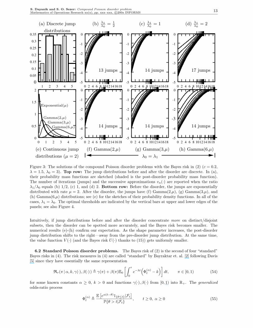
S. Dayanik and S. O. Sezer: Compound Poisson disorder problemMathematics of Operations Research xx(x), pp. xxx–xxx, c©200x INFORMS 13
14 jumps14 jumps
17 jumps14 jumps13 jumps
λ0 = λ1
Gamma(3,µ)
Gamma(6,µ)
Gamma(2,µ)
distributions
(a) Discrete jump (b) λ1λ0
= 12
(c) λ1λ0
= 1 (d) λ1λ0
= 2
Exponential(µ)
(h) Gamma(6,µ)(g) Gamma(3,µ)(f) Gamma(2,µ)
distributions (µ = 2)
(e) Continuous jump
14 jumps
0 -5
0
-1
-2
-4
-5-5
-4
-3
-2
-1
0
-5
0
-1
-2
-3
-4
-5
-5
-4
-3
2
1.5
1
0.5
0
0.05
0.1
-2
-1
00
-1
-2
-3
-4
0.3
0.25
0.2
0.15
1 2 43 5 0 2 1816141210864 0 18161412108642
0.35
0 18161412108642
888 12141618 1210 16181 2 3 4 5
0
-3
-2
-1
0
1210 1416186420146420106420
-3
-4
Figure 3: The solutions of the compound Poisson disorder problems with the Bayes risk in (2) (c = 0.2,λ = 1.5, λ0 = 3). Top row: The jump distributions before and after the disorder are discrete. In (a),their probability mass functions are sketched (shaded is the post-disorder probability mass function).The number of iterations (jumps) and the successive approximations vn(·) are reported when the ratioλ1/λ0 equals (b) 1/2, (c) 1, and (d) 2. Bottom row: Before the disorder, the jumps are exponentiallydistributed with rate µ = 2. After the disorder, the jumps have (f) Gamma(2,µ), (g) Gamma(3,µ), and(h) Gamma(6,µ) distributions; see (e) for the sketches of their probability density functions. In all of thecases, λ1 = λ0. The optimal thresholds are indicated by the vertical bars at upper and lower edges of thepanels; see also Figure 4.
Intuitively, if jump distributions before and after the disorder concentrate more on distinct/disjointsubsets, then the disorder can be spotted more accurately, and the Bayes risk becomes smaller. Thenumerical results (e)-(h) confirm our expectation. As the shape parameter increases, the post-disorderjump distribution shifts to the right—away from the pre-disorder jump distribution. At the same time,the value function V (·) (and the Bayes risk U(·) thanks to (15)) gets uniformly smaller.
6.2 Standard Poisson disorder problems. The Bayes risk of (2) is the second of four “standard”Bayes risks in (4). The risk measures in (4) are called “standard” by Bayraktar et. al. [2] following Davis[5] since they have essentially the same representation
Rτ (π |α, k, γ(·), β(·) ) , γ(π) + β(π)E0
[∫ τ
0
e−λt(Φ(α)
t − k)]
dt, π ∈ [0, 1) (54)
for some known constants α ≥ 0, k > 0 and functions γ(·), β(·) from [0, 1) into R+. The generalizedodds-ratio process
Φ(α)t ,
E[eα(t−θ)1θ≤t|Ft
]Pθ > t|Ft
, t ≥ 0, α ≥ 0 (55)

14 S. Dayanik and S. O. Sezer: Compound Poisson disorder problemMathematics of Operations Research xx(x), pp. xxx–xxx, c©200x INFORMS
(h) Gamma(6,µ)(g) Gamma(3,µ)(f) Gamma(2,µ)
(d) λ1λ0
= 2(c) λ1λ0
= 1(b) λ1λ0
= 12
0131197531
0
5
10
15
20
17151311975310
5
10
15
20
1715131197531
0
5
10
15
20
17151311975310
5
10
15
20
17151311975310
5
10
15
20
1715131197531
17
20
15
10
5
15
Figure 4: The critical thresholds ξn, n = 1, 2, . . . for the compound Poisson disorder problems consideredin Figure 3
becomes the same as the odds-ratio process Φt, t ≥ 0 in (11) when α = 0. If we redefine the parametera in (12) by
a , λ + α− λ1 + λ0,
then the process Φ(α) = Φ(α)t ; t ≥ 0 has the same dynamics as in (13) for every α ≥ 0:
Φ(α)t = x
(t− σn−1,Φ(α)
σn−1
), t ∈ [σn−1, σn)
Φ(α)σn
=λ1
λ0f(Yn)Φ(α)
σn−
, n ≥ 1.
See Bayraktar et. al. [2, Proposition 2.1] for the proof of the following result.
Proposition 6.1 For every π ∈ [0, 1) and stopping time τ ∈ F, we have
R(i)τ (π) = Rτ (π|αi, ki, γi(·), βi(·)), for every i = 1, 2, 3, 4, (56)
where α1 = α2 = α3 = 0, α4 = α; k1 = (λ/c)e−ελ, k2 = λ/c, k3 = 1/c, k4 = λ/(cα); and
γ1(π) = (1− π)e−λε, γ2(π) = 1− π, γ3(π) =1− π
λ, γ4(π) = 1− π
β1(π) = c(1− π), β2(π) = c(1− π), β3(π) = c(1− π), β4(π) = cα(1− π).
For i = 2 the identity in (54, 56) is the same as the representation (10) which was the key for thesolution. Therefore, the solution of the compound Poisson disorder problem with any “standard” Bayesrisk in (4,56) remains the same after a few obvious changes.
The minimum Bayes risk U(π) = infτ∈F R(π|α, k, γ(·), β(·)), π ∈ [0, 1) is given by
U(π) = γ(π) + β(π) V
(π
1− π
), π ∈ [0, 1)

S. Dayanik and S. O. Sezer: Compound Poisson disorder problemMathematics of Operations Research xx(x), pp. xxx–xxx, c©200x INFORMS 15
λ1
λ0= 1
2
(d) R(4), α = 1(c) R(3)(a) R(2)
11 jumps 11 jumps 10 jumps 10 jumps
10 jumps 8 jumps 6 jumps 8 jumps
λ1
λ0= 2
(b) R(1), ε = 0.1λ
0 0 2 4 6 8 10-4
-3.5-3
-2.5-2
-1.5-1
-0.50
0 2 4 6 8 10-4
-3.5-3
-2.5-2
-1.5-1
-0.50
0 2 4 6 8 10
-4-3.5
-3-2.5
-2-1.5
-1-0.5
0
-4-3.5
-3-2.5
-2-1.5
-1-0.5
0
-4-3.5
-3-2.5
-2-1.5
-1-0.5
0
-0.5-1
-1.5-2
-2.5-3
-3.5-4
108642
0
Figure 5: As in Bayraktar, Dayanik, and Karatzas [2], we take c = 0.2, λ = 1.5, λ0 = 3 and ν0(·) ≡ ν1(·) ≡δ1(·). For each case, the rate λ1 is determined according to the ratio λ1/λ0 at the beginning of the samerow. In every column, the disorder problem is solved for one of four penalties (linear, ε, expected miss, andexponential). The number of iterations (jumps) before convergence and the successive approximationsvn(·) of the value function V (·) are displayed for eight cases. In every case, the optimal threshold ξn foreach subproblem vn(·) is indicated by a vertical bar on both top and bottom edges of the panels; see alsoFigure 6.
in terms of the value function
V (φ) , infτ∈F
Eφ0
[∫ τ
0
e−λtg(Φ(α)t )dt
], φ ∈ R+
of a discounted optimal stopping problem with the running cost
g(φ) , φ− k, φ ∈ R+
and discount rate λ > 0 for the piecewise-deterministic Markov process Φ(α) in (55). The successiveapproximations Vn(·)n≥1 in (19) of the value function V (·) are uniformly decreasing; and since g(·) ≥−k, we have
−k
λ·(
λ0
λ + λ0
)n
≤ V (φ)− Vn(φ) ≤ 0.
The results of Sections 3-5 remain valid in this general case.
Figure 5 illustrates solutions of some Poisson disorder problem for each of four “standard” Bayes riskmeasures in (4). For comparison the parameters are chosen the same as in Bayraktar et. al. [2, Table1], whose methods are unable to detect the change in the jump-size distribution, and therefore, can onlyuse the count data on the number of arrivals to detect the disorder. On the other hand, the method ofSections 3-5 can be told to ignore completely the jump-size information (and to use number of arrivalsonly) by setting the density function f(·) in (8) and (13) identically to one (more precisely, the jump-distributions ν0(·) and ν1(·) are replaced with the Dirac measure δ1(·) at one on R+, so that the processX is the same as the counting process N in (1)). In Figure 5, the rightmost vertical bars at the edge ofpanels mark the critical thresholds of the quickest alarm rules and agree with those reported by Bayraktaret. al. [2, Table 1].

16 S. Dayanik and S. O. Sezer: Compound Poisson disorder problemMathematics of Operations Research xx(x), pp. xxx–xxx, c©200x INFORMS
(d) R(4), α = 1(b) R(1), ε = 0.1λ (c) R(3)(a) R(2)
λ1
λ0= 2
λ1
λ0= 1
2
115310
2
4
6
8
10
11975310
2
4
6
8
10
11975310
2
4
6
8
10
1197531
11975310
2
4
6
8
10
11975310
2
4
6
8
10
11975310
2
4
6
8
10
1197531
97
Figure 6: The critical thresholds ξn, n = 1, 2, . . . for the standard Poisson disorder problems consideredin Figure 5.
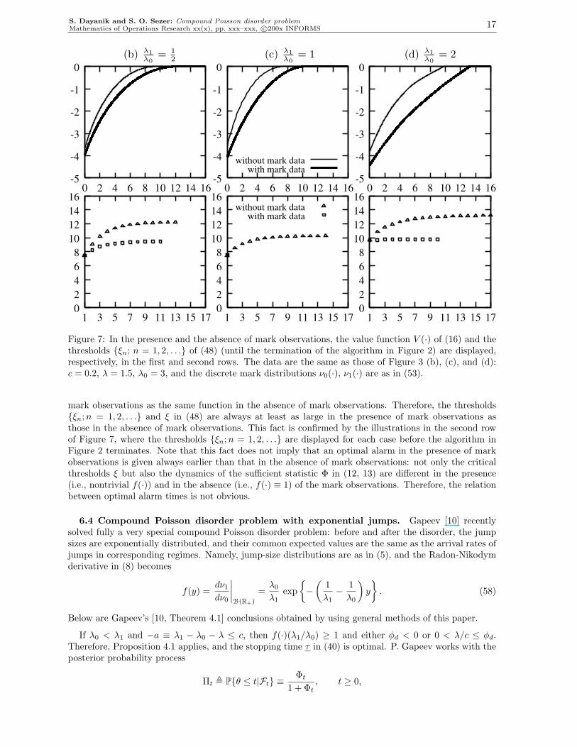
6.3 Reducing the Bayes-risk by observing marks in addition to arrival times. Supposethat in the examples (b)-(d) of Figure 3 the observations of marks are unavailable, and one has to useonly the data on the arrival times in order to detect the disorder time. How do the optimal Bayes risksand optimal strategies differ?
For different values of the ratio λ1/λ0, the value function of (16) is calculated in the presence and theabsence of the mark data and displayed in the first row of Figure 7. In the absence of the mark data,compound Poisson disorder problem reduces to standard Poisson disorder problem, and the solutions ofthe latter are recalled from Figure 5(a) for λ1/λ0 = 1/2 and 2.
If λ1/λ0 = 1, and the mark data is absent, then (i) the sufficient statistic Φ in (11-13) becomes theincreasing deterministic process
Φt = x(t, Φ0) = −1 + eλt [Φ0 + 1] , t ≥ 0 (λ0 = λ1, f(·) ≡ 1), (57)
(ii) following from (16, 17, 19)), the optimal thresholds in (49) become ξ1 = ξ2 = . . . = ξ = λ/c, (iii) theoptimal alarm time t∗(Φ0) = inft ≥ 0 : Φt ≥ λ/c is also deterministic,
t∗(Φ0) =[
1λ
ln(
1 + (λ/c)1 + Φ0
)]+and V (φ) =
1 + φ
λ
[1 + ln
(1 + (λ/c)
1 + φ
)]− λ + c
cλ.
The latter expression is used to draw the graph in Figure 7(b) of the value function V (·) of (16) corre-sponding to the case without mark observations.
The first row of Figure 7 shows that the reduction in the Bayes risk obtained by using the observationsof the marks (in addition to those of the arrival times) can be significant. Moreover, this reduction tendsto grow as the number of arrivals (hence the additional information carried by the accompanying markdata) increases with the increasing rate λ1 for fixed λ0. Finally, observe from (57) that arrival times carryno information about the disorder time if the arrival rate is not expected to change (i.e., λ0 = λ1), andthe observations of marks become more crucial for early detection of the disorder and for lower Bayesrisk; see Figure 7(b).
Since every stopping time of the arrival process N = Nt; t ≥ 0 in (1) is also a stopping timeof X = Xt; t ≥ 0, the value function V (·) of (19) is always at least as small in the presence of
S. Dayanik and S. O. Sezer: Compound Poisson disorder problemMathematics of Operations Research xx(x), pp. xxx–xxx, c©200x INFORMS 17
(d) λ1λ0
= 2(c) λ1λ0
= 1(b) λ1λ0
= 12
-5
-1
0
0 2 4 6 8 10 12 14 16-5
-4
-3
-2
-1
0
0 2 4 6 8 10 12 14 16
with mark data-5
-4
-3
-2
-1
0
0 2 4 6 8 10 12 14 16
02468
10121416
171513119753102468
10121416
1715131197531
without mark datawith mark data
02468
10121416
1715131197531
without mark data
-3
-4
-2
Figure 7: In the presence and the absence of mark observations, the value function V (·) of (16) and thethresholds ξn; n = 1, 2, . . . of (48) (until the termination of the algorithm in Figure 2) are displayed,respectively, in the first and second rows. The data are the same as those of Figure 3 (b), (c), and (d):c = 0.2, λ = 1.5, λ0 = 3, and the discrete mark distributions ν0(·), ν1(·) are as in (53).
mark observations as the same function in the absence of mark observations. Therefore, the thresholdsξn;n = 1, 2, . . . and ξ in (48) are always at least as large in the presence of mark observations asthose in the absence of mark observations. This fact is confirmed by the illustrations in the second rowof Figure 7, where the thresholds ξn;n = 1, 2, . . . are displayed for each case before the algorithm inFigure 2 terminates. Note that this fact does not imply that an optimal alarm in the presence of markobservations is given always earlier than that in the absence of mark observations: not only the criticalthresholds ξ but also the dynamics of the sufficient statistic Φ in (12, 13) are different in the presence(i.e., nontrivial f(·)) and in the absence (i.e., f(·) ≡ 1) of the mark observations. Therefore, the relationbetween optimal alarm times is not obvious.
6.4 Compound Poisson disorder problem with exponential jumps. Gapeev [10] recentlysolved fully a very special compound Poisson disorder problem: before and after the disorder, the jumpsizes are exponentially distributed, and their common expected values are the same as the arrival rates ofjumps in corresponding regimes. Namely, jump-size distributions are as in (5), and the Radon-Nikodymderivative in (8) becomes
f(y) =dν1
dν0
∣∣∣∣B(R+)
=λ0
λ1exp
−(
1λ1− 1
λ0
)y
. (58)
Below are Gapeev’s [10, Theorem 4.1] conclusions obtained by using general methods of this paper.
If λ0 < λ1 and −a ≡ λ1 − λ0 − λ ≤ c, then f(·)(λ1/λ0) ≥ 1 and either φd < 0 or 0 < λ/c ≤ φd.Therefore, Proposition 4.1 applies, and the stopping time τ in (40) is optimal. P. Gapeev works with theposterior probability process
Πt , Pθ ≤ t|Ft ≡Φt
1 + Φt, t ≥ 0,

18 S. Dayanik and S. O. Sezer: Compound Poisson disorder problemMathematics of Operations Research xx(x), pp. xxx–xxx, c©200x INFORMS
and the optimal stopping rule τ can be rewritten as
τ = inf
t ≥ 0 : Πt ≥λ
λ + c
.
If either “λ0 < λ1 and −a > c” or λ0 > λ1, then the stopping rule U0 = inft ≥ 0 : Φt ≥ ξ = inft ≥0 : Πt ≥ ξ/(1+ξ) in (36, 45, 48, 49) is optimal by Propositions 3.11 and 5.1. If λ0 > λ1, then φd < 0 andthe value function V (·) in (16) is continuously differentiable on R+ by Lemma 7.1 below, and V ′(ξ) = 0.
7. Differentiability and variational inequalities. In this final section, smoothness of the valuefunction V (·) in (16) is studied. The function V (·) is shown to be piecewise continuously differentiableand unique bounded solution of the variational inequalities in (18); see Lemma 7.1 and Proposition 7.3on pages 20 and 21, respectively.
7.1 Differentiability of the value function. Since V (·) ≡ 0 on the stopping region Γ = [ξ,∞) by(45, 48, 49), it is obviously continuously differentiable on (ξ,∞). Its smoothness on [0, ξ] is investigatedbelow separately in two cases due to different behavior of functions t 7→ x(t, φ), φ ∈ R+ of (12) forφd /∈ (0, ξ] and φd ∈ (0, ξ]. We summarize our conclusions in Lemma 7.1.
In both case, it will be very useful to recall from Remark 3.10 and (34, 35, 45, 49) that the valuefunction V (·) satisfies some form of dynamic programming equation; namely,
V (φ) = JV (t, φ) + e−(λ+λ0)tV (x(t, φ)), t ∈ [0, r(φ)], (59)r(φ) = inft > 0 : x(t, φ) ≥ ξ, φ ∈ R+
Case I: φd /∈ (0, ξ]. Let us fix some φ ∈ [0, ξ) and define for every 0 < h < ξ − φ that
T (h, φ) , inft ≥ 0 : x(t, φ) ≥ φ + h =
1a· ln(
φ + h− φd
φ− φd
), a 6= 0
h/λ, a = 0
.
The second equality follows from (12). Because T (h, φ) ≤ r(φ), replacing T (h, φ) with t in (59) gives
V (φ) =∫ T (h,φ)
0
e−(λ+λ0)u [g + λ0 · SV ] (x(u, φ))du + e−(λ+λ0)T (h,φ)V (φ + h). (60)
Subtracting V (φ + h) from each side and dividing by −1/h give
V (φ + h)− V (φ)h
= − 1h
∫ T (h,φ)
0
e−(λ+λ0)u [g + λ0 · SV ] (x(u, φ)du
− 1h
[e−(λ+λ0)T (h,φ) − 1
]V (φ + h).
Since V (·) is concave by Corollary 3.4 and Proposition 3.6, it has right derivatives everywhere. As hdecreases to 0, we obtain
limh→0+
V (φ + h)− V (φ)h
= −(g(φ) + λ0 · SV (φ)− (λ + λ0)V (φ)
)·(
∂T (h, φ)∂h
∣∣∣∣h=0
), (61)
since the functions V (·) and SV (·) are bounded and continuous (by bounded convergence theorem).Because
∂T (h, φ)∂h
∣∣∣∣h=0
=
1/[a(φ− φd)
], a 6= 0
1/λ, a = 0
=
1λ + aφ
(62)
is a continuous function of φ ∈ [0, ξ) (recall that φd /∈ [0, ξ), so the denominator is bounded away fromzero on φ ∈ [0, ξ)), the right derivative of V (·) in (61) is continuous on φ ∈ [0, ξ). Since V (·) is concave,this implies that V (·) is continuously differentiable on [0, ξ), and (61, 62) give the derivative
V ′(φ) =g(φ) + λ0 · SV (φ)− (λ + λ0)V (φ)
λ + aφ, φ ∈ [0, ξ). (63)
Finally, V ′(ξ−) = 0 = V ′(ξ+) since V (·) ≡ 0 on [ξ,∞) and [g + λ0 · SV ](ξ) = 0 because of Corollary5.2(ii) and φd /∈ [0, ξ). The concavity of V (·) implies again that V ′(ξ) exists and equals zero. Hence thefunction V (·) is continuously differentiable everywhere on R+ if φd /∈ [0, ξ).
S. Dayanik and S. O. Sezer: Compound Poisson disorder problemMathematics of Operations Research xx(x), pp. xxx–xxx, c©200x INFORMS 19
Case II: φd ∈ (0, ξ]. For every φ ∈ R+, the function x(t, φ) converges monotonically to φd as tincreases to infinity. For every φ ∈ [0, ξ), we have V (φ) = JV (∞, φ) by Corollary 5.2(ii).
If we redefine T (h, φ) , inft ≥ 0 : |x(t, φ) − φ| ≥ h for every φ ∈ [0, ξ) and h > 0, then the samearguments as in the previous case show that V (·) is continuously differentiable (with the same derivativeV ′(φ) as in (63)) on φ ∈ [0, ξ) \ φd.
Let us show now that the function V (φ) is not differentiable at φ = ξ. In terms of
W (φ) , [g + λ0 · SV ](φ), φ ∈ R+,
one can write using Corollary 5.2(ii) that
V (ξ)− V (ξ − h)h
=∫ ∞
0
e−(λ+λ0)u
[W(x(u, ξ)
)−W
(x(u, ξ − h)
)x(u, ξ)− x(u, ξ − h)
]·
[x(u, ξ)− x(u, ξ − h)
h
]du.
Since the functions g(·) and V (·) are increasing, so are SV (·) of (25) and W (·). Therefore,
W(x(u, ξ)
)−W
(x(u, ξ − h)
)x(u, ξ)− x(u, ξ − h)
≥ 0 andx(u, ξ)− x(u, ξ − h)
h= eau;
and Fatou’s Lemma gives
limh→0+
V (ξ)− V (ξ − h)h
≥∫ ∞
0
e−λ1u
[1 + λ0 lim
h→0+
SV(x(u, ξ)
)− SV
(x(u, ξ − h)
)x(u, ξ)− x(u, ξ − h)
]du.
Since SV (·) is increasing, the limit infimum above is non-negative and
limh→0+
V (ξ)− V (ξ − h)h
≥∫ ∞
0
e−λ1udu =1λ1
> 0 = limh→0+
V (ξ + h)− V (ξ)h
. (64)
Hence, the lefthand and righthand derivatives of V (·) are unequal at φ = ξ, and V (·) is not differentiableat φ = ξ.
On the other hand, the function V (·) may or may not be differentiable at φ = φd. Since x(t, φd) = φd
for every t ≥ 0 by (12), Corollary 5.2(ii) gives
V (φd + h)− V (φd)h
=1λ1
+ λ0
∫ ∞
0
e−(λ+λ0)uSV (φd + eauh)− SV (φd)
hdu.
Because SV (·) is nondecreasing, Fatou’s lemma gives
limh→0+
V (φd + h)− V (φd)h
≥ 1λ1
+ λ0
∫ ∞
0
e−(λ+λ0)u[
limh→0+
SV (φd + eauh)− SV (φd)h
]du. (65)
We shall calculate the limit infimum on the righthand side. In terms of the sets
A ,
y ∈ Rd; f(y)λ1
λ0= 1
and B ,
y ∈ Rd; f(y)λ1
λ0φd = ξ
, (66)
the definition in (25) of SV (·) implies
SV (φd + eauh)− SV (φd)h
=∫
Rd\(A∪B)
ν0(dy)
[V(f(y)λ1
λ0(φd + eauh)
)− V
(f(y)λ1
λ0φd
)h
]
+∫
A
ν0(dy)[V (φd + eauh)− V (φd)
h
]+∫
B
ν0(dy)[V (ξ + (ξ/φd)eauh)− V (ξ)
h
].
The last integral is equal to 0 because V (φ) = 0 for every φ ≥ ξ. Since the concave and increasing functionV (·) has bounded right derivatives by Corollary 3.4 and is continuously differentiable on R+ \ φd, ξ,the dominated convergence theorem implies that
limh→0+
SV (φd + eauh)− SV (φd)h
= eau λ1
λ0
∫Rd\(A∪B)
ν1(dy)V ′(f(y)
λ1
λ0φd
)+ eauν0(A). lim
h→0+
V (φd + h)− V (φd)h
for every u ∈ R+. (67)

20 S. Dayanik and S. O. Sezer: Compound Poisson disorder problemMathematics of Operations Research xx(x), pp. xxx–xxx, c©200x INFORMS
Inside the integral above, we used the relation f(y)ν0(dy) = ν1(dy). After plugging (67) into (65),rearrangement of the terms gives[
limh→0+
V (φd + h)− V (φd)h
]·(
1− λ0
λ1ν0(A)
)≥ 1
λ1+∫
Rd\(A∪B)
ν1(dy)V ′(
f(y)λ1
λ0φd
).
Similar arguments will also give[lim
h→0+
V (φd + h)− V (φd)h
]·(
1− λ0
λ1ν0(A)
)≤ 1
λ1+∫
Rd\(A∪B)
ν1(dy)V ′(
f(y)λ1
λ0φd
).
Since φd ∈ (0, ξ] in Case II, we have a < 0, λ0 < λ1, and [1−(λ0/λ1)ν0(A)] > 0. By the last two displayedinequalities, the righthand derivative D+V (φ) of V (·) at φ = φd becomes
D+V (φd) =(
1− λ0
λ1ν0(A)
)−1[
1λ1
+∫
Rd\(A∪B)
ν1(dy)V ′(f(y)
λ1
λ0φd
)].
By following the same arguments, one can show that the lefthand derivative D−V (φ) of V (·) at φ = φd
becomes
D−V (φd) = D+V (φd) +(
1− λ0
λ1ν0(A)
)−1 [λ0ξ
λ1φdν0(B) D−V (ξ)
].
Since the derivative D−V (ξ) on the right does not vanish by (64), this equality shows that the valuefunction V (·) is differentiable at φ = φd (i.e., D−V (φd) = D+V (φd)) if and only if ν0(B) = 0 for the setB defined in (66). Next lemma summarizes main conclusions.
Lemma 7.1 Recall from (45, 48, 49) that the optimal continuation region for the problem (16) is in theform of C = [0, ξ) for some ξ > 0, and the constant φd is given by (12).
(i) If φd /∈ C = [0, ξ), then the value function V (·) in (16) is continuously differentiable on R+.
(ii) If φd ∈ C = [0, ξ), then V (·) is continuously differentiable on R+ \φd, ξ. It is not differentiableat ξ. It is differentiable at φd if and only if
ν0
(y ∈ Rd; f(y)
λ1
λ0φd = ξ
)= 0.
Remark 7.2 If φd ∈ C, then V (φd) < 0. The local martingale in (38) and optional sampling imply that
V (φd) = Eφd
0
[∫ σ1
0
e−λtg(Φ)dt + eλσ1V (Φσ1)]
=g(φd)λ + λ0
+λ0
λ + λ0· SV (φd),
since the process Φ does not leave φd until the first jump time σ1 if it starts initially at φd. This relationof SV (φd) of (25) to V (φd) and Lemma 7.1(ii) suggest that the lack of smoothness of V (·) at φd canoccur if and only if this “ill” behavior can be “transmitted” from ξ. Alternatively, the function V (·)is not differentiable at φd if and only if the process Φ may jump before the disorder from φd to ξ withpositive probability.
7.2 Unique solution of variational inequalities. The value function V (·) satisfies the variationalinequalities in (18) wherever V (·) is differentiable. By Proposition 5.1,
V < 0 on C = [0, ξ) and V = 0 on Γ = R+ \C. (68)
The function V (·) is piecewise continuously differentiable by Lemma 7.1. The derivative V ′(·) exists andequals zero on the stopping region Γ. Since V (·) ≡ 0 on Γ and A , x ∈ R+ : [g + λ0 · SV ](x) < 0 ⊆ Cby Lemma 5.2, we have
(A− λ)V (φ) + g(φ) = [g + λ0 · SV ](φ) ≥ 0 on φ ∈ Γ = [ξ,∞).
The above inequality is strict in the interior of Γ because φ 7→ [g + λ0 · SV ](φ) is strictly increasing. Atevery point φ ∈ C where the derivative V ′(φ) exists (see Lemma 7.1 above), it is given by (63) which canbe rearranged as
0 = (λ + aφ)V ′(φ) + λ0SV (φ)− (λ + λ0)V (φ) + g(φ)
= [λ + aφ]V ′(x) + λ0
∫y∈Rd
[V
(λ1
λ0f(y) φ
)− V (φ)
]ν0(dy)− λV (φ) + g(φ)
= (A− λ)V (φ) + g(φ).
(69)
S. Dayanik and S. O. Sezer: Compound Poisson disorder problemMathematics of Operations Research xx(x), pp. xxx–xxx, c©200x INFORMS 21
It is easy to see from (68-69) that V (·) satisfies the variational inequalities in (18) wherever the derivativeV ′(·) exists. Next result shows that V (·) is the unique piecewise continuously differentiable boundedsolution of (18).
Proposition 7.3 Suppose that U : R+ 7→ R is a continuous and bounded function which is continuouslydifferentiable except at most finitely many points and satisfies (18) everywhere except at those points.Then U = V on R+.
Proof. Let T be any F-stopping time and t ≥ 0 be any constant. As in Appendix A.3,
e−λ(T∧t)U(ΦT∧t)− U(Φ0) =∫ T∧t
0
e−λs(A− λ)U(Φs−)ds
+∫
(0,T∧t]×Rd
e−λs
[U
(λ1
λ0f(y)Φs−
)− U(Φs−)
]q0(dsdy).
Since U(·) is bounded, the integrand of the last integral on the right is absolutely integrable with respectto the (P0, F)-compensator measure p0(dsdy) = λ0ds ν0(dy). Therefore, the last integral on the right is amartingale, and its P0-expectation equals zero. Taking the P0-expectations of both sides and using theinequality (A− λ)U + g ≥ 0 give
U(φ) ≤ Eφ0
[e−λ(T∧t)U(ΦT∧t)
]+ Eφ
0
[∫ T∧t
0
e−λsg(Φs)ds
]. (70)
Since U(·) is bounded and g(·) + λ/c ≥ 0, the bounded convergence and monotone convergence theoremsgive U(φ) ≤ Eφ
0
[∫ T
0e−λsg(Φs)
]when we take limit of both sides as t goes to infinity. Since F-stopping
time T is arbitrary, this implies U ≤ V .
For the opposite inequality, let T∗ , inft ≥ 0 : U(Φt) = 0. Then [(A− λ)U + g](Φs) = 0 for s < T∗,and (70) holds with equality. When we take the limits as before, we obtain U(φ) = Eφ
0
[∫ T∗0
e−λsg(Φs)]≥
V (φ) for every φ ∈ R+.
Acknowledgments. We are grateful to the referee, the associate and area editors for their detailedsuggestions, which improved our presentation. The work is supported by the National Science Foundation,under grant NSF-DMI-04-23327.
Appendix.
A.1 Absolutely continuous change of measure. The process X in (1) can also be expressed asthe integral
Xt = X0 +∫
(0,t]×Rd
y p(dsdy), t ≥ 0 (A.71)
with the respect to the point process
p((0, t]×A) ,∞∑
k=1
1σk≤t1Yk∈A, t ≥ 0, A ∈ B(Rd) (A.72)
on(R+ × Rd,B(R+)⊗B(Rd)
). Let P0 be the probability measure described in Section 2 and define
h(t, y) , 1t<θ + 1t≥θλ1
λ0f(y), t ∈ R+, y ∈ Rd.
Since θ is G0-measurable, the process h(t, y); t ≥ 0 is G-predictable for every y ∈ Rd. Therefore, theprocess
Zt , exp
∫(0,t]×Rd
[lnh(s, y)]p(dsdy)−∫
(0,t]×Rd
[h(s, y)− 1]λ0 ds ν0(dy))
, t ≥ 0
is a (P0, G)-martingale and induces a new probability measure P on the measurable space (Ω,∨s≥0Gs)in terms of the Radon-Nikodym derivatives (9). The exponential formula for Zt above also simplifies tothat in (9). Girsanov theorem for the point processes (Jacod and Shiryaev [12, Chapter III], Cont andTankov [4, p. 305]) guarantees that, under the new probability measure P, the process X has the desiredfinite-dimensional distribution described in the introduction.

22 S. Dayanik and S. O. Sezer: Compound Poisson disorder problemMathematics of Operations Research xx(x), pp. xxx–xxx, c©200x INFORMS
A.2 The dynamics of the odds-ratio process Φ in (11). The Radon-Nikodym derivative Zt in(9) of the restriction to Gt of the probability measure P with respect to that of P0 can be written as
Zt = 1θ>t + 1θ≤tLt
Lθ, where Lt , e−(λ1−λ0)t
Nt∏k=1
[λ1
λ0f(Yk)
], t ≥ 0 (A.73)
is the likelihood ratio process. The process L = Lt; t ≥ 0 is the unique locally bounded solution of thedifferential equation (Elliott [8, p. 155])
dLt = Lt−
[−(λ1 − λ0)dt +
∫y∈Rd
(λ1
λ0f(y)− 1
)p(dtdy)
], t ≥ 0 (L0 = 1), (A.74)
where p(·) is the point process in (A.72). Since the random variable θ is independent of the process Xand has the exponential distribution in (6) under P0, the generalized Bayes theorem (Shiryaev [16, pp.230-231]) and (A.73) give
Φt =E[1θ≤t|Ft]Pτ > θ|Ft
=E0[Zt1θ≤t|Ft]
E0[Zt|Ft]
(E0[Zt1θ>t|Ft]E0[Zt|Ft]
)−1
=eλt
1− πE0
[Lt
Lθ1θ≤t
∣∣∣∣Ft
]=
eλt
1− π
[πLt + (1− π)
∫ t
0
λe−λu Lt
Ludu
]≡ π
1− πUt + Vt
in terms of
Ut , eλtLt and Vt ,∫ t
0
λeλ(t−u) Lt
Ludu.
Using the change-of-variable formula (Protter [15, p. 78], Jacod and Shiryaev [12, p. 57], Cont and Tankov[4, p. 277]) and the dynamics of the process L in (A.74) give
dUt = Ut−
[(λ− λ1 + λ0)dt +
∫y∈Rd
(λ1
λ0f(y)− 1
)p(dtdy)
], U0 = 1,
dVt = λdt + Vt−
[(λ− λ1 + λ0)dt +
∫y∈Rd
(λ1
λ0f(y)− 1
)p(dtdy)
], V0 = 0.
Therefore, the dynamics of the process Φ = [π/(1− π)] · U + V are
dΦt = [λ + (λ− λ1 + λ0)Φt] dt + Φt−
∫y∈Rd
[λ1
λ0f(y)− 1
]p(dtdy), t ≥ 0,
Φ0 =π
1− π.
(A.75)
The stochastic differential equation in (A.75) can be solved pathwise and explicitly for Φ. Let theparameters a = λ− λ1 + λ0, φd = −λ/a be defined as in (12) and let x(·, φ) = x(t, φ); t ∈ R, φ ∈ R bethe unique solution (given explicitly in (12)) of the ordinary differential equation
d
dtx(t, φ) = λ + ax(t, φ), t ∈ R and x(0, φ) = φ. (A.76)
As clearly seen from (A.75), the process Φ follows the integral curves of the differential equation in (A.76)between consecutive jumps of X and is updated instantaneously at every jump of X as summarized in(13).
A.3 The infinitesimal generator of the process Φ. The dynamics of Φ in (A.75) and the(P0, F)-compensator measure p0(dsdy) = λ0dsν0(dy) of the point process p(·) in (A.72) determine the(P0, F)-infinitesimal generator of the process Φ. Let a = λ− λ1 + λ0 as in (12), and h : R+ 7→ R be any
S. Dayanik and S. O. Sezer: Compound Poisson disorder problemMathematics of Operations Research xx(x), pp. xxx–xxx, c©200x INFORMS 23
locally bounded continuously differentiable function. Then
h(Φt)− h(Φ0) =∫ t
0
(λ + aΦs−) h′(Φs−)ds +∫
(0,t]×Rd
[h
(λ1
λ0f(y)Φs−
)− h(Φs−)
]p(dsdy)
=∫ t
0
(λ + aΦs−) h′(Φs−)ds +∫
(0,t]×Rd
[h
(λ1
λ0f(y)Φs−
)− h(Φs−)
]p0(dsdy)
+∫
(0,t]×Rd
[h
(λ1
λ0f(y)Φs−
)− h(Φs−)
]q0(dsdy)
=∫ t
0
(λ + ax) h′(x) + λ0
∫Rd
[h
(λ1
λ0f(y)x
)− h(x)
]ν0(dy)
∣∣∣∣x=Φs−
ds
+∫
(0,t]×Rd
[h
(λ1
λ0f(y)Φs−
)− h(Φs−)
]q0(dsdy).
The last integral with respect to the compensated random measure q0(·) = p0(·) − p0(·) is a (P0, F)-local martingale. Therefore, the integrand of the last Lebesgue integral equals the (P0, F)-infinitesimalgenerator (Ah) Φs− composed with the process Φ; see (14).
A.4 Long proofs. For the proof of Proposition 3.5, we shall need the following result on the char-acterization of F-stopping times; see Bremaud [3, Theorem T33, p. 308], Davis [7, Lemma A2.3, p. 261].
Lemma A.1 For every F-stopping time τ and every n ∈ N0, there is an Fσn-measurable random variableRn : Ω 7→ [0,∞] such that τ ∧ σn+1 = (σn + Rn) ∧ σn+1 P0-a.s. on τ ≥ σn.
Proof of Proposition 3.5. First, we shall establish the inequality
Eφ0
∫ τ∧σn
0
e−λtg(Φt
)dt ≥ vn(φ), τ ∈ F, φ ∈ R+ (A.77)
for every n ∈ N0, by proving inductively on k = 1, . . . , n + 1 that
Eφ0
[∫ τ∧σn
0
e−λtg(Φt
)]dt
≥ Eφ0
[∫ τ∧σn−k+1
0
e−λtg(Φt
)dt + 1τ≥σn−k+1e
−λσn−k+1vk−1
(Φσn−k+1
)]=: RHSk−1. (A.78)
Observe that (A.77) follows from (A.78) when we set k = n + 1.
If k = 1, then the inequality (A.78) is satisfied as an equality since v0 ≡ 0. Suppose that (A.78) holdsfor some 1 ≤ k < n + 1. We shall prove that it must also hold when k is replaced with k + 1. Let usdenote the righthand side of (A.78) by RHSk−1, and rewrite it as
RHSk−1 = RHS(1)k−1 + RHS
(2)k−1 , Eφ
0
[∫ τ∧σn−k
0
e−λtg(Φt
)dt
]+ Eφ
0
[1τ≥σn−k
(∫ τ∧σn−k+1
σn−k
e−λtg(Φt
)dt + 1τ≥σn−k+1e
−λσn−k+1vk−1
(Φσn−k+1
))](A.79)
where we used∫ τ∧σn−k+1
0=
∫ τ∧σn−k
0+1τ≥σn−k
∫ τ∧σn−k+1
τ∧σn−k, as well as 1τ≥σn−k1τ≥σn−k+1 =
1τ≥σn−k+1. By Lemma A.1, there is an Fσn−k-measurable random variable Rn−k such that τ∧σn−k+1 =
(σn−k + Rn−k) ∧ σn−k+1 P0-almost surely on τ ≥ σn−k. Therefore, the second expectation, denotedby RHS
(2)k−1, in (A.79) becomes
Eφ0
1τ≥t
[∫ (t+Rn−k)∧s
t
e−λtg(Φt
)dt + 1t+Rn−k≥se
−λsvk−1
(Φs
)]∣∣∣∣∣t=σn−ks=σn−k+1
= Eφ0
1τ≥σn−ke
−λσn−kfn−k(Rn−k,Φσn−k)

24 S. Dayanik and S. O. Sezer: Compound Poisson disorder problemMathematics of Operations Research xx(x), pp. xxx–xxx, c©200x INFORMS
by the strong Markov property of X, where fk−1(r, φ) equals
Eφ0
[∫ r∧σ1
0
e−λtg(Φt
)dt + 1r≥σ1e
−λσ1vk−1
(Φσ1
)]= Jvk−1(r, φ) ≥ J0vk−1(φ) = vk(φ).
The (in)equalities follow from (21), (22) and (23), respectively. Thus
RHS(2)k−1 ≥ Eφ
0
[1τ≥σn−ke
−λσn−kvk
(Φσn−k
)].
From (A.78) and (A.79), we finally obtain
Eφ0
[∫ τ∧σn
0
e−λtg(Φt
)dt
]≥ RHSk−1 = Eφ
0
[∫ τ∧σn−k
0
e−λtg(Φt
)dt
]+ RHS
(2)k−1
≥ Eφ0
[∫ τ∧σn−k
0
e−λtg(Φt
)dt + 1τ≥σn−ke
−λσn−kvk
(Φσn−k
)]= RHSk.
This completes the proof of (A.78) by induction on k, and (A.77) follows by setting k = n + 1 in (A.78).When we take the infimum of both sides in (A.77), we obtain Vn ≥ vn, n ∈ N.
The opposite inequality Vn ≤ vn, n ∈ N follows immediately from (29) since every F-stopping time Sεn
is less than or equal to σn, P0-a.s. by construction. Therefore, we only need to establish (29). We willprove it by induction on n ∈ N. For n = 1, the lefthand side of (29) becomes Eφ
0
[∫ Sε1
0e−λtg
(Φt
)dt]
=
Eφ0
[∫ rε0(φ)∧σ1
0e−λtg
(Φt
)dt]
= Jv0(rε0(φ), φ). Since Jv0(rε
0(φ), φ) ≤ J0v0(φ) + ε by Remark 3.2, theinequality (29) holds for n = 1.
Suppose that (29) holds for every ε > 0 for some n ∈ N. We will prove that it also holds when n isreplaced with n + 1. Since Sε
n+1 ∧ σ1 = rε/2n
(Φ0
)∧ σ1, P0-a.s., we have
Eφ0
[∫ Sεn+1
0
e−λtg(Φt
)dt
]= Eφ
0
[∫ Sεn+1∧σ1
0
e−λtg(Φt
)dt + 1Sε
n+1≥σ1
∫ Sεn+1
σ1
e−λtg(Φt
)dt
]
= Eφ0
[∫ rε/2n (φ)∧σ1
0
e−λtg(Φt
)dt + 1rε/2
n (φ)≥σ1
∫ σ1+Sε/2n θσ1
σ1
e−λtg(Φt
)dt
]
= Eφ0
[∫ rε/2n (φ)∧σ1
0
e−λtg(Φt
)dt
]+ Eφ
0
[1rε/2
n (φ)≥σ1e−λσ1fn
(Φσ1
)]by strong Markov property of X, where fn(φ) , Eφ
0
[∫ Sε/2n
0e−λtg
(Φt
)dt]≤ vn(φ)+ ε/2. by the induction
hypothesis. Therefore, Eφ0
[∫ Sεn+1
0e−λtg
(Φt
)dt]
is less than or equal to
Eφ0
[∫ rε/2n (φ)∧σ1
0
e−λtg(Φt
)dt + 1rε/2
n (φ)≥σ1e−λσ1vn
(Φσ1
)]+
ε
2= Jvn(rε/2
n (φ), φ) +ε
2.
However, Jvn(rε/2n (φ), φ) ≤ vn+1(φ) + ε/2 by Remark 3.2. The last two inequalities prove (29) when n is
replaced with n + 1.
Proof of Lemma 3.7. Let us fix a constant u ≥ t and φ ∈ R+. Then
Jw(u, φ) = Eφ0
[(∫ t∧σ1
0
+1σ1>t
∫ u∧σ1
t
)e−λsg(Φs)ds + 1u≥σ1e
−λσ1w(Φσ1)]
. (A.80)
On the event σ1 > t, we have u ∧ σ1 = [t + (u − t)] ∧ [t + σ1 θt] = t + [(u − t) ∧ σ1 θt]. Therefore,the strong Markov property of X gives
Eφ0
[1σ1>t
∫ u∧σ1
t
e−λsg(Φs)ds
]= Eφ
0
[1σ1>te
−λtEΦt0
[∫ (u−t)∧σ1
0
e−λsg(Φs)ds
]]= Eφ
0
[1σ1>te
−λt(Jw(u− t, Φt)− EΦt
0
[1u−t≥σ1e
−λσ1w(Φσ1)] )]
= e−(λ+λ0)t Jw(u− t, x(t, φ)
)− Eφ
0
[1σ1>t1u≥σ1e
−λσ1w(Φσ1)].
(A.81)
S. Dayanik and S. O. Sezer: Compound Poisson disorder problemMathematics of Operations Research xx(x), pp. xxx–xxx, c©200x INFORMS 25
The second equality follows from the definition of Jw in (21), and the last from (13) and the strongMarkov property. Substituting (A.81) into (A.80) gives
Jw(u, φ) = Eφ0
[∫ t∧σ1
0
e−λsg(Φs)ds + 1t≥σ1e−λσ1w(Φσ1)
]+ e−(λ+λ0)t Jw
(u− t, x(t, φ)
)= Jw(t, φ) + e−(λ+λ0)t Jw
(u− t, x(t, φ)
).
Finally, taking the infimum of both sides over u ∈ [t, +∞] proves (30).
Proof of Proposition 3.11. Note that the sequence of random variables
∫ Uε∧σn
0
e−λsg(Φs)ds + e−λ(Uε∧σn)V (ΦUε∧σn) ≥ −2∫ ∞
0
e−λs λ
cds = −2
c
is bounded from below; see (16). By (39) and Fatou’s Lemma, we have
V (φ) ≥ Eφ0
[lim
n→∞
(∫ Uε∧σn
0
e−λsg(Φs)ds + e−λ(Uε∧σn)V (ΦUε∧σn)
)]
= Eφ0
[∫ Uε
0
e−λsg(Φs)ds + 1Uε<∞e−λUεV (ΦUε)
]
≥ Eφ0
[∫ Uε
0
e−λsg(Φs)ds
]− ε Eφ
0
[1Uε<∞e
−λUε]≥ Eφ
0
[∫ Uε
0
e−λsg(Φs)ds
]− ε
for every φ ∈ R+. This concludes the proof.
Proof of Proposition 3.12. First, let us show (39) for n = 1. Fix ε ≥ 0 and φ ∈ R+. ByLemma A.1, there exists a constant u ∈ [0,∞] such that Uε ∧ σ1 = u ∧ σ1. Then
Eφ0 [MUε∧σ1 ] = Eφ
0
[∫ u∧σ1
0
e−λsg(Φs)ds + 1u≥σ1e−λσ1V (Φσ1)
]+ Eφ
0
[1u<σ1e
−λuV (Φu)]
= JV (u, φ) + e−(λ+λ0)uV(x(u, φ)
)= JuV (φ), (A.82)
where the second equality follows from (21) and (13), and the last from (33).
Fix any t ∈ [0, u). By (33) and (13),
JV (t, φ) = JtV (φ)− e−(λ+λ0)tV (x(t, φ))
≥ J0V (φ)− e−(λ+λ0)tV (x(t, φ)) = J0V (φ)− Eφ0
[1σ1>te
−λtV (Φt)].
On the event σ1 > t, we have Uε > t (otherwise, Uε ≤ t < σ1 would imply Uε = u ≤ t, whichcontradicts with our initial choice of t < u). Thus, V (Φt) < −ε on σ1 > t. Hence, JV (t, φ) > J0V (φ)+ε Eφ
0
[1σ1>te
−λt]
= J0V (φ) + ε e−(λ+λ0)u ≥ J0V (φ) for every t ∈ [0, u). Therefore, J0V (φ) = JuV (φ),and (A.82) implies Eφ
0 [MUε∧σ1 ] = JuV (φ) = J0V (φ) = V (φ) = Eφ0 [M0]. This completes the proof of (39)
for n = 1.
Now suppose that (39) holds for some n ∈ N, and let us show the same equality for n + 1. Note thatEφ
0 [MUε∧σn+1 ] = Eφ0 [1Uε<σ1MUε ] + Eφ
0 [1Uε≥σ1MUε∧σn+1 ] equals
Eφ0 [1Uε<σ1MUε ] + Eφ
0
[1Uε≥σ1
∫ σ1
0
e−λsg(Φs)ds
]+ Eφ
0
[1Uε≥σ1
∫ Uε∧σn+1
σ1
e−λsg(Φs)ds + e−λ(Uε∧σn+1)V (ΦUε∧σn+1)
].
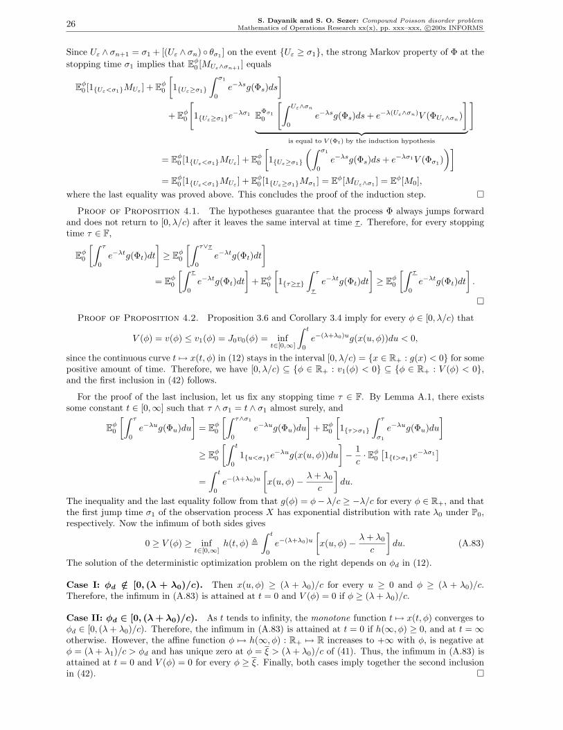
26 S. Dayanik and S. O. Sezer: Compound Poisson disorder problemMathematics of Operations Research xx(x), pp. xxx–xxx, c©200x INFORMS
Since Uε ∧ σn+1 = σ1 + [(Uε ∧ σn) θσ1 ] on the event Uε ≥ σ1, the strong Markov property of Φ at thestopping time σ1 implies that Eφ
0 [MUε∧σn+1 ] equals
Eφ0 [1Uε<σ1MUε ] + Eφ
0
[1Uε≥σ1
∫ σ1
0
e−λsg(Φs)ds
]+ Eφ
0
[1Uε≥σ1e
−λσ1 EΦσ10
[∫ Uε∧σn
0
e−λsg(Φs)ds + e−λ(Uε∧σn)V (ΦUε∧σn)
]︸ ︷︷ ︸
is equal to V (Φt) by the induction hypothesis
]
= Eφ0 [1Uε<σ1MUε ] + Eφ
0
[1Uε≥σ1
(∫ σ1
0
e−λsg(Φs)ds + e−λσ1V (Φσ1))]
= Eφ0 [1Uε<σ1MUε ] + Eφ
0 [1Uε≥σ1Mσ1 ] = Eφ[MUε∧σ1 ] = Eφ[M0],where the last equality was proved above. This concludes the proof of the induction step.
Proof of Proposition 4.1. The hypotheses guarantee that the process Φ always jumps forwardand does not return to [0, λ/c) after it leaves the same interval at time τ . Therefore, for every stoppingtime τ ∈ F,
Eφ0
[∫ τ
0
e−λtg(Φt)dt
]≥ Eφ
0
[∫ τ∨τ
0
e−λtg(Φt)dt
]= Eφ
0
[∫ τ
0
e−λtg(Φt)dt
]+ Eφ
0
[1τ≥τ
∫ τ
τ
e−λtg(Φt)dt
]≥ Eφ
0
[∫ τ
0
e−λtg(Φt)dt
].
Proof of Proposition 4.2. Proposition 3.6 and Corollary 3.4 imply for every φ ∈ [0, λ/c) that
V (φ) = v(φ) ≤ v1(φ) = J0v0(φ) = inft∈[0,∞]
∫ t
0
e−(λ+λ0)ug(x(u, φ))du < 0,
since the continuous curve t 7→ x(t, φ) in (12) stays in the interval [0, λ/c) = x ∈ R+ : g(x) < 0 for somepositive amount of time. Therefore, we have [0, λ/c) ⊆ φ ∈ R+ : v1(φ) < 0 ⊆ φ ∈ R+ : V (φ) < 0,and the first inclusion in (42) follows.
For the proof of the last inclusion, let us fix any stopping time τ ∈ F. By Lemma A.1, there existssome constant t ∈ [0,∞] such that τ ∧ σ1 = t ∧ σ1 almost surely, and
Eφ0
[∫ τ
0
e−λug(Φu)du
]= Eφ
0
[∫ τ∧σ1
0
e−λug(Φu)du
]+ Eφ
0
[1τ>σ1
∫ τ
σ1
e−λug(Φu)du
]≥ Eφ
0
[∫ t
0
1u<σ1e−λug(x(u, φ))du
]− 1
c· Eφ
0
[1t>σ1e
−λσ1]
=∫ t
0
e−(λ+λ0)u
[x(u, φ)− λ + λ0
c
]du.
The inequality and the last equality follow from that g(φ) = φ− λ/c ≥ −λ/c for every φ ∈ R+, and thatthe first jump time σ1 of the observation process X has exponential distribution with rate λ0 under P0,respectively. Now the infimum of both sides gives
0 ≥ V (φ) ≥ inft∈[0,∞]
h(t, φ) ,∫ t
0
e−(λ+λ0)u
[x(u, φ)− λ + λ0
c
]du. (A.83)
The solution of the deterministic optimization problem on the right depends on φd in (12).
Case I: φd /∈ [0, (λ + λ0)/c). Then x(u, φ) ≥ (λ + λ0)/c for every u ≥ 0 and φ ≥ (λ + λ0)/c.Therefore, the infimum in (A.83) is attained at t = 0 and V (φ) = 0 if φ ≥ (λ + λ0)/c.
Case II: φd ∈ [0, (λ + λ0)/c). As t tends to infinity, the monotone function t 7→ x(t, φ) converges toφd ∈ [0, (λ + λ0)/c). Therefore, the infimum in (A.83) is attained at t = 0 if h(∞, φ) ≥ 0, and at t = ∞otherwise. However, the affine function φ 7→ h(∞, φ) : R+ 7→ R increases to +∞ with φ, is negative atφ = (λ + λ1)/c > φd and has unique zero at φ = ξ > (λ + λ0)/c of (41). Thus, the infimum in (A.83) isattained at t = 0 and V (φ) = 0 for every φ ≥ ξ. Finally, both cases imply together the second inclusionin (42).

S. Dayanik and S. O. Sezer: Compound Poisson disorder problemMathematics of Operations Research xx(x), pp. xxx–xxx, c©200x INFORMS 27
References
[1] Erhan Bayraktar and Savas Dayanik, Poisson disorder problem with exponential penalty for delay,Mathematics of Operations Research. To appear, 2005.
[2] Erhan Bayraktar, Savas Dayanik, and Ioannis Karatzas, The standard Poisson disorder problemrevisited, Stochastic Process. Appl. 115 (2005), no. 9, 1437–1450. MR MR2158013
[3] Pierre Bremaud, Point Processes and Queues, Springer-Verlag, New York, 1981, Martingale dynam-ics, Springer Series in Statistics. MR 82m:60058
[4] Rama Cont and Peter Tankov, Financial Modelling with Jump Processes, Chapman & Hall/CRCFinancial Mathematics Series, Chapman & Hall/CRC, Boca Raton, FL, 2004. MR MR2042661
[5] M. H. A. Davis, A note on the Poisson disorder problem, Banach Center Publ. 1 (1976), 65–72.[6] , Piecewise-deterministic Markov processes: a general class of nondiffusion stochastic models,
J. Roy. Statist. Soc. Ser. B 46 (1984), no. 3, 353–388, With discussion. MR 87g:60062[7] , Markov Models and Optimization, Monographs on Statistics and Applied Probability,
vol. 49, Chapman & Hall, London, 1993. MR 96b:90002[8] Robert J. Elliott, Stochastic Calculus and Applications, Applications of Mathematics (New York),
vol. 18, Springer-Verlag, New York, 1982. MR MR678919 (85b:60059)[9] L. I. Galchuk and B. L. Rozovskii, The disorder problem for a Poisson process, Theory of Prob. and
Appl. 16 (1971), 729–734.[10] Pavel V. Gapeev, The disorder problem for compound Poisson processes with exponential jumps,
Ann. Appl. Probab. 15 (2005), no. 1A, 487–499. MR MR2115049[11] U. S. Gugerli, Optimal stopping of a piecewise-deterministic Markov process, Stochastics 19 (1986),
no. 4, 221–236. MR 88j:60084[12] Jean Jacod and Albert N. Shiryaev, Limit Theorems for Stochastic Processes, second ed.,
Grundlehren der Mathematischen Wissenschaften [Fundamental Principles of Mathematical Sci-ences], vol. 288, Springer-Verlag, Berlin, 2003. MR 2003j:60001
[13] Goran Peskir and Albert N. Shiryaev, Solving the Poisson disorder problem, Advances in financeand stochastics, Springer, Berlin, 2002, pp. 295–312. MR 2003i:60071
[14] H. Vincent Poor, An Introduction to Signal Detection and Estimation, second ed., Springer Texts inElectrical Engineering, Springer-Verlag, New York, 1994, A Dowden & Culver Book. MR MR1270019(95c:94004)
[15] Philip E. Protter, Stochastic Integration and Differential Equations, second ed., Applications ofMathematics (New York), vol. 21, Springer-Verlag, Berlin, 2004, Stochastic Modelling and AppliedProbability. MR MR2020294
[16] A. N. Shiryaev, Probability, Graduate Texts in Mathematics, vol. 95, Springer-Verlag, New York,1996. MR 97c:60003
[17] Albert N. Shiryaev, A remark on the quickest detection problems, Statist. Decisions 22 (2004), no. 1,79–82. MR MR2065992
Related Documents