Composition and abundance of freshwater fish communities

1

Composition and abundance of

freshwater fish communities across a

land use gradient in Sabah, Borneo

Clare Wilkinson

September 2013

A thesis submitted in partial fulfilment of the requirements for the degree

of Master of Science and Diploma of Imperial College London

© Clare Wilkinson

© Clare Wilkinson © Clare Wilkinson

“In all works on Natural History, we constantly find details of the marvellous adaptation of animals to

their food, their habits, and the localities in which they are found”. Alfred Russel Wallace

2

Declaration of own work

I declare that this thesis (insert full title)

Composition and abundance of freshwater fish communities across a

land use gradient in Sabah, Borneo

is entirely my own work and that where material could be construed as the

work of others, it is fully cited and referenced, and/or with appropriate

acknowledgement given.

Signature ……………………………………………………..

Name of student: Clare Wilkinson

Name of Supervisor: Dr. Robert Ewers

3

CONTENTS

1. INTRODUCTION…………………………………………………………...9

1.1. Tropical freshwater fish diversity……………………………………..9

1.2. Threats to freshwater fish in Borneo………………………………...10

1.3. The Stability of Altered Forest Ecosystems (SAFE) Project………10

1.4. Project aims and objectives…………………………………………..11

2. BACKGROUND…………………………………………………………...12

2.1. Capture Mark Recapture of Freshwater fish……………………….12

2.1.1. Sampling and tagging methods……………………………………...12

2.1.2. Modelling fish abundance……………………………………………13

2.2. Freshwater fish in Borneo……………………………………………15

2.2.1. Overview of species…………………………………………………..15

2.2.2. Role in tropical forest streams……………………………………….16

2.3. Effects of land use change on freshwater fish in Borneo………...16

2.3.1. Logging………………………………………………………………...16

2.3.2. Conversion…………………………………………………………...18

2.4. Study Site: A land use gradient in Eastern Sabah, Borneo……..19

2.4.1. Yayasan Sabah Concession Area…………………………………19

2.4.2. Virgin Jungle Reserve……………………………………………….20

2.4.3. Benta Wawasan Oil Palm plantation………………………………20

3. METHODS………………………………………………………………....21

3.1. Framework……………………………………………………………..21

3.2. Data Collection………………………………………………………..21

3.2.1. Project design and location………………………………………….21

3.2.2. Trapping………………………………………………………………..22

3.2.3. Tagging protocol………………………………………………………23

3.2.4. Forest quality variables in the riparian zone……………………….24

3.2.5. Stream variables………………………………………………………25

3.3. Data analyses…………………………………………………………26

3.3.1. Dispersal……………………………………………………………….26

3.3.2. Abundance estimation………………………………………………...26

4

3.3.3. Comparison of abundance across the land use gradient………….28

3.3.4. Methodological comparison…………………………………………..29

3.3.5. Community level comparisons across the land use gradient……..29

4. RESULTS…………………………………………………………………..31

4.1. Fish dispersal…………………………………………………………..31

4.2. Indices if land use gradient…………………………………………...32

4.3. Population modelling and estimation………………………………..33

4.4. Comparison of abundance across the land use gradient…………34

4.5. Methodological comparison………………………………………….37

4.6. Community similarity and species turnover rates………………….39

5. DISCUSSION……………………………………………………………...43

5.1. Response of fish to logging and conversion to oil palm…………..43

5.1.1. Species level…………………………………………………………..43

5.1.2. Community level………………………………………………………45

5.2. Dispersal……………………………………………………………….48

5.3. Capture Mark Recapture of fish……………………………………..48

5.4. Review of fish capture techniques at SAFE………………………..50

5.5. Project limitations and further research…………………………….51

5.5.1. Project design…………………………………………………………51

5.5.2. Land use variables……………………………………………………52

5.5.3. Capture Mark Recapture……………………………………………..53

5.6. Conclusion…………………………………………………………….54

6. REFERENCES……………………………………………………………55

7. APPENDICES…………………………………………………………….65

I – Model selection by species/site in Mark………………………...65

II – GLM Abundance estimate model selection……………………67

III – Effects of year and land use on relative species abundance.69

5

LIST OF FIGURES

Figure 2.1: Map of the study site……………………………………………….. .11

Figure 3.1: Fish trapping methods, a) bottle trap, b) cast net……………….. .15

Figure 4.1: Dispersal a)all fish, b)N. everetti c)T. dourensis d)Rasbora……..23

Figure 4.2: PCA of riparian vegetation divides streams by land use…………24

Figure 4.3: Modelled abundance against land use indices……………………28

Figure 4.4: Comparison of trapping methods for focal taxa…………………...30

Figure 4.5: Multivariate ordination using PCoA of sites and species…………32

Figure 4.6: Absolute species turnover rates against indices of land use…….36

LIST OF TABLES

Table 3.1: Variables measured to indicate vegetation quality……………….17

Table 3.2: Models used to estimate abundance………………………………20

Table 4.1: Abundance estimates of focal taxa…………………………………26

Table 4.2: Results of mixed effects models comparing trapping methods…29

6

LIST OF ACRONYMS

AIC Akaike’s Information Criterion

AICc Akaike’s Information Criterion corrected

ANOVA Analysis Of Variance

CMR Capture Mark Recapture

DBH Diameter at Breast Height

DVCA Danum Valley Conservation Area

GLM Generalised Linear Model

LF Logged Forest

OG Old growth (forest)

OP Oil Palm

PC1 Principle Component 1

PCA Principle Component Analysis

PCoA Principle Co-ordinates Analysis

PIT Passive Integrated Transponder

SAFE Stability of Altered Forest Ecosystems

VJR Virgin Jungle Reserve

7

ABSTRACT

Malaysia has the highest levels of deforestation and production of palm oil

around the world. Due to the paucity of data on the ichthyofauna of Sabah,

understanding how this affects the diversity and abundance of freshwater fish,

is of great interest as levels of deforestation and conversion to oil palm

increase. This project used capture-mark-recapture to determine the

abundance and dispersal of three focal taxa (N. everetti, Tor dourensis,

Rasbora). Relative abundance was used to compare community similarity and

absolute species turnover rates, across the land use gradient. 200m stream

transects were established in old growth forest, logged forest and oil palm

catchments as part of the Stability of Altered Forest Ecosystems project.

Abundance of three focal taxa decreased as riparian vegetation and stream

quality decreased; despite this the highest abundance estimate was in oil

palm. Community analysis demonstrated a slight, albeit non-significant

difference between sampling years (p=0.054) and land use (p=0.098)

between sites, and relative abundance of species varied by year and land

use. Results need to be treated cautiously due to low recaptures rates and a

degree of over-dispersion in the data. The difference indicated over a land use

gradient is corroborated, but alternate hypotheses are somewhat divided in

the literature, as suggestions of differences at the mesohabitat scale and

possible barriers to migration need to be further investigated. It is

recommended that intensive research is conducted to obtain a full species list,

for the area in order to fully assess how logging and conversion affects fish

diversity and abundance in the short and long term. A critical assessment of

trapping methodologies was undertaken and recommendations as to the use

of trapping techniques are made accordingly.

Word count: 14,929

8

ACKNOWLEDGMENTS

I would like to thank the SAFE project and the Sime Darby Foundation for

funding this project and allowing it to happen.

I extend great thanks to Dr. Rob Ewers, for giving me this opportunity,

supervising this project and providing invaluable advice in the field and during

the write-up.

All fieldwork was made possible by the SAFE project staff, who make working

in challenging conditions, not only possible, but fun and wanting to do more.

Minsheng and Sarah co-ordinated logistics, enabling research to run smoothly

and to schedule, whilst research assistants Sabri, James, Maria and Opong

are pro’s with a cast net, taught me Malay and enabled fieldwork to not only

happen but successfully catch nearly 3,000 fish and a terrapin! I could not

have completed field work without Rosa Gleave. She provided for support

throughout and made me laugh or a cup of tea after the hardest day’s

fieldwork.

Data contributions and priceless information were contributed from Victoria

Bignet, Sarah Luke, Holly Barclay and Anand Nainar. This enabled data and

relationships to be further explored.

Data analysis was made enjoyable by the great help of Jack Thorley and the

Silwood computer room. I would like to thank Beth Thomas and Sara Eckert

for reading drafts of the thesis, providing advice and cakes throughout the

time of write up.

9

1. INTRODUCTION

Tropical rainforest ecosystems contain two-thirds of the world’s terrestrial

biodiversity (Gardener et al., 2009) but are one of the most threatened

ecosystems on the planet (FAO, 2006). Borneo lies within the Sunderland

hotspot and regrettably has the highest deforestation rates around the world

(Sodhi et al., 2010), with annual rates of deforestation reaching 1.3% (FAO,

2010). This deforestation has resulted in a matrix of degraded forest and

agricultural estates, with little primary forest existing outside forest reserves

and protected areas (McMorrow and Talip, 2001). In addition a shift in

agricultural practices for further economic gain now sees the highest levels of

palm oil production in Malaysia and Indonesia, in the world. Oil palm

plantations cover 1.2 million ha in the Malaysian state of Sabah in North

Borneo, with more being created on degraded, selectively logged, secondary

forest (McMorrow and Talip, 2001; Bradshaw et al., 2009; Bruhl and Eltz,

2010). Forest degradation and the increasing demand for palm oil are

accelerating forest loss. These factors, compounded with few studies

addressing the effects on biodiversity, concerns conservationists and

ecologists around the world (Laurance et al., 2012).

1.1. Tropical freshwater fish diversity

The majority of the world's freshwater fish biodiversity is contained within

tropical regions (Lowe-McConnell, 1987; Kottelat et al., 1993; Kottelat and

Whitten, 1996). Almost 10,000 species of freshwater fishes are currently

recognised (Nelson, 1994) with many more species awaiting discovery and

description (Kottelat and Whitten, 1996). The tropics of South-East Asia

possess less fish species than that of South America, but have a greater

diversity in the number of families (Kottelat et al., 1993). Malaysia (including

the states of Sabah and Sarawak in Borneo) is in the top 10 countries for

highest freshwater fish diversity, with more than 600 described species

(Kottelat and Whitten, 1996). Despite these figures, the ichthyofauna of Asia,

and particularly Borneo, remains patchy because of concentrations of studies

in easily accessible areas. The Kalabakan basin, where this project takes

10

place, is not well documented due to a lack of appropriate species counts and

descriptions (Dudgeon, 2000; Martin-Smith, 1998b).

1.2. Threats to freshwater fish in Borneo

As figures above state, logging and conversion to oil palm in Sabah is

continuing and increasing at an unprecedented rate. A number of projects

have studied forest fragmentation and deforestation (Lovejoy et al., 1983;

Casant et al., 2002; Ritters et al., 2000) but few have directly quantified the

effects of fragmentation and land use change on tropical forest ecosystems

(Ewers et al,. 2011), and fewer still have focused on fish. It is therefore

essential to be able to draw comparisons between land uses, on the effects

on biodiversity at the species and community level.

The removal of tropical forest cover during timber extraction represents an

extreme form of disturbance, with potentially far-reaching effects on fish

biodiversity. Positive and negative effects have been observed on freshwater

fish abundance and community diversity across different land uses (Martin-

Smith, 1998a; Iwato et al., 2005; Nunakawa, 2005). A number of hypotheses

are therefore presented: altered allochthonous inputs and solar regulation

(Nunakawa, 2005), mesohabitats (Martin-Smith, 1998b) and significant

barriers to migration (Martin-Smith and Laird, 1998). The lack of corroboration

between studies strengthens the need to understand the impact land use

change has on freshwater fish. Until now, no study has been conducted to

quantify species abundance or community composition between streams

covered by the SAFE project.

1.3 The Stability of Altered Forest Ecosystems (SAFE) Project

The SAFE project is one of the largest, established ecological experiments

investigating responses of biodiversity to land use change and fragmentation

(Ewers et al., 2011). Based in Sabah, Malaysia, the SAFE project’s principal

aim is to quantify the effects of logging, deforestation and fragmentation on

the biodiversity and physical processes intrinsic to tropical forests. The project

makes use of the planned expansion of oil palm activities over time. While the

focus may be on the responses of forest fragmentation and conversion, the

11

SAFE project has been working on the biological impacts deforestation has

on riparian strips. A group of six small, headstream catchments, currently in

continuous logged forest have been instrumented and transects set up. The

SAFE project has planned manipulations in the future riparian strip after

conversion to oil palm, translating to differences in percentage forest cover in

each catchment. The Brantian Tantulit Virgin Jungle Reserve, the nearby oil

palm estates of Selangan Batu and Merbau, and continuous logged forest

outside the experimental area will act as unlogged primary forest, established

oil palm plantation and logged forest control sites, respectively.

1.4. Project Aims and objectives

This project aims to use capture-mark-recapture (CMR) to investigate the

impact forest modification has on freshwater fish population abundance and

composition. The main objectives are to:

1. Use CMR data to calculate the rate and extent of dispersal of fish to

determine if such studies are justifiable.

2. Compare the abundance of three focal fish species across the land

use gradient at the SAFE project.

3. Utilise previous data collected to compare the species turnover rates

and community similarity of streams, across the land use gradient.

4. Critically assess the trapping methods used at the SAFE project

(cast netting and bottle trapping), for catching fish.

12

2. BACKGROUND

2.1 Capture Mark Recapture of Freshwater Fish

2.1.1 Sampling and tagging methods

Scientists and managers of fish populations need to be able to collect reliable

data, through all environmental conditions in order to understand populations

and increase predictive capabilities for successful management (Barbour et

al., 2011). Sampling methods vary in skill and technical ability to catch fish,

from electrofishing using two electrodes to pass a current through water, to

traditional line and net methods. Electrofishing has short and long term

problems, including immediate and delayed mortality (Neilson, 1998) which is

not an option when sampling endangered species. Whereas, traditional

methods may target specific species when attempting to monitor a whole

stream community, through the chosen net size or the mesohabitat it is used

in (Martin-Smith, 1998a; 1998b). Both of these methods enable CMR, one of

the most widespread tools for monitoring to be used, and a variety of methods

exist in order to do this (Barbour et al. 2011; Pine et al. 2003).

CMR methods are used for estimating the population size and survival

parameters of fish populations (Pine et al., 2003). CMR methods can take the

form of chemical, internal (PIT, radio tags) or external marks (floy, streamer

tags, fin clips and dyes) each with there own advantages and disadvantages.

The methods vary over: the number of fish that can be tagged, the cost to

implement such a study, the information that can be determined about the

population and the fate of tagged fish (Barbour et al., 2011; Pine et al., 2003).

The majority of marking methods require individuals to be physically captured

in order to be marked and recaptured to ‘read’ the tag. Traps can be set along

stream or river transects, and need to be monitored over several trapping

occasions. This may be carried out over successive days if determining

abundance estimates or longer periods if further population parameters (for

example survival and recruitment) are desired (Cooch and White, 2011). The

simplest estimates of abundance can be calculated over two trapping

occasions. On the first, individuals within a population are caught, marked,

and released at the point of capture. After the determined time length (often

13

the next day) the same method is used to re-sample the population. It is noted

which animals already have a mark, and unmarked individuals are marked.

Repeating this process over multiple trapping occasions allows capture

histories (1’s if encountered and 0’s if not encountered for each capture

occasion) to be created for each individual, forming the basis of CMR models.

As mentioned, many different methods can be used to tag fish. Passive

integrated transponder (PIT) tags, introduced in the 1980s have substantially

increased in popularity (Gibbons and Andrews, 2004). Tags are implanted

internally, are available in a range of sizes (6-32mm length), allow for

individual identification and are relatively low cost allowing for a high number

of individuals to be tagged (Barbour et al., 2011). PIT tags are ideal for long-

term studies as they have no battery and very long life spans (Gibbons and

Andrews, 2004). A benefit of PIT tags is that they give flexibility in recapture

methods; through physical recapture or integration with telemetry or

autonomous antenna detection systems and both have been successfully

applied in freshwater environments (Jepsen et al., 2000; Muir et al., 2001;

Sandford and Smith, 2002). Disadvantages include low retention rates for

some species (Barrowman and Myers, 1996) and sparse data outputs that are

typical of traditional CMR studies if physical recapture is required (Adams et

al., 2006). The benefit of individual identification outweighs these negatives,

making pit tagging a good option for conducting a mark recapture study in

headstreams in Borneo.

2.1.2 Modelling fish abundance

Modelling the abundance of fish is dependent upon the efficiency of sampling

methods and model assumptions being adhered to. Freshwater fish studies

typically have low efficiency of sampling methods (Bayley and Austin, 2002)

and very low recapture rates which affect the accuracy and precision of

models (Pine et al., 2003). It is because of this that studies need to clearly

plan fieldwork, to maximise capture efficiencies, and ensure model

assumptions are met.

14

Abundance of sampled populations can be explored and quantified using a

variety of models that fall into two broad categories, open- or closed- capture

models, each with different assumptions (Cooch and White, 2011). Closed-

capture models assume the sampled population has no immigration,

emigration, births or deaths during the study period (Otis et al., 1978; White et

al., 1982), whereas open-capture models allow the population to change in

size and composition over the duration of the study (Lettink and Armstrong,

2003). Closed-capture models can be used over short time periods for

monitoring freshwater fish, if the major assumption of population closure has

to be met (Pine et al., 2003; Lettink and Armstrong, 2003). Open-capture

models can be used if closure cannot be met. The major assumptions of open

models include: the equal catchability of marked and unmarked individuals at

each sampling occasion, tags are not lost, tags are read properly, sampling is

instantaneous, survival probabilities are the same for all individuals between

each sampling occasion and the study area is constant (Cooch and White,

2012; Pine et al., 2003).

The parameters of simple open-capture models that are applied to sampled

populations include: p – the probability of capture of both marked and

unmarked animals, phi – the survival probability of both marked and

unmarked animals between occasions, b – the probability of entrance into the

population and t – time (Cooch and White, 2012). These parameters are used

to estimate N, the initial population size of the sampled population. The

parameters can be manipulated allowing the user to consider biologically

relevant characteristics of animals. The most parsimonious model is sort, to

find the optimal compromise between precision and bias, as this model will be

the best fit to the data and only parameters that are useful in explaining the

data will remain (Burnham and Anderson 2002). This is based on the model

likelihood, Akaike Information Criterion (AIC) value and number of model

parameters (Akaike, 1974; Burnham and Anderson, 2004). Multiple models

may be plausible and the estimate of population abundance can be weighed

in relation to these criteria.

15

2.2 Freshwater fish in Borneo

2.2.1 Overview of species

Despite the lack of information on freshwater fish in Borneo mentioned earlier,

other catchments in Sabah adjacent to this project site have been sampled

and species lists compiled (For example: Danum Valley by Martin-Smith and

Tan, (1998); Kinabatangan by Lim and Wong, (1994); Lower Kinabatagan

earlier this year near Danau Girang Field Centre). Martin-Smith and Tan

(1998b) document finding 65 different species in the Danum valley, Lower

Segama and Upper Kuamut Rivers with the Family Cyprinidae dominating the

diversity. New taxa have been described from the Kalabakan catchment area

(Tan, 2006) and a previous three month study at the SAFE project in 2011,

caught over 2000 fish of 18 different species in 12 different genera (Bignet,

Pers. Comms.). This indicates the high diversity in the region, as species

accumulation curves have long tails, suggesting rare species can be found

opportunistically over time (Martin-Smith, 1998b). However, significant

differences are shown between regions and catchments separated by small

geographical distances (Martin-Smith, 1998b).

The species diversity is dominated by the cyprinid family (Inger and Kong,

2002). Cyprinids vary in size and diet, from detritivores to active predators and

are commonly caught in cast nets in smaller streams (Martin-Smith and Tan,

1998). The most interesting group of endemic fish are the ‘sucker fish’, found

in rocky, fast-flowing streams. These fish feed on the algae on rocks and

comprise the genera Gastromyzon, Glaniopsis, Protomyzon and

Neogastromyzon (Inger and Kong, 2002).

Methods for capture of all species may be biased to certain species, for

example cast netting for pool dwelling Cyprinids, but less so for ‘sucker fish’,

due to the differences in vertical distribution within the water column of

streams. Methods must therefore be diversified in order to obtain a picture of

the whole stream community.

16

2.2.2 Role in tropical forest streams

The relationship between freshwater fish abundance and distributions, and the

physical habitat, have been investigated in a range of temperate environments

(Chipps et al., 1994), but remain largely unexplored in tropical communities

(Martin-Smith, 1998a). However, fish do play important roles in tropical

streams (Chipps et al., 1994), and it is accepted that detrital and algal-feeding

fish are widespread in tropical streams which contrasts to the insectivorous

fish that predominate in temperate streams (Flecker, 1992). These fish can

affect the invertebrate assemblage by modifying the distribution and

abundance of resources available to them (Flecker, 1992), thus impacting the

whole stream biota. Martin-Smith (1998a) comments on the sharp

discontinuities that can exist in small streams giving rise to distinct habitats,

that fish species commonly show preferences towards, giving rise to

differences in species assemblages.

Several additional roles have been suggested for freshwater fish. Firstly, that

frugivorous fish have a possible role in seed dispersal in the neo-tropics (Horn

et al., 2011). Secondly, that fish could have a role as useful bio-indicators of

water quality and pollution levels (Ahmad and Shuihami-Othman, 2010) as

forests are logged and converted to oil palm.

These roles raise the profile of the potential use of freshwater fish in studies

investigating stream quality, health and in studies comparing land use. This is

coupled with a general lack of knowledge about tropical fish rarity, abundance

and effects of land use change.

2.3 Effects of land use change on freshwater fish in Borneo

2.3.1 Logging

There are four main categories of human induced threat to fish: flow alteration

or regulation, pollution, catchment alteration and overharvesting (Dudgeon,

2000). These cause streams to lose integrity, frequently resulting in less

diversity and lower productivity of the ecological communities involved

(Pringle et al., 2000; Jackson et al., 2001; Jungwirth et al., 2002). Logging and

deforestation is a form of catchment alteration, causing changes in water flow

17

and dramatic increases in sedimentation (Iwata et al., 2003; Inoue et al.,

2003). These physical and hydrological modifications have been studied to

some extent in the tropics, but the effects on freshwater fish remains poorly

understood (Martin-Smith, 1998a).

Due to extensive deforestation in the tropics (Archard et al., 2002), the last 25

years has seen a substantial research effort demonstrating that stream

ecosystem maintenance is dependent upon land use regimes (Naiman et al.,

2000). Riparian forests have a strong influence on the abundance, distribution

and assemblage of fish, particularly in headwater and low order streams

(Inoue, 2005). Woody debris can alter the channel and provide cover and

different habitats (Inoue and Nakano, 1998); whereas root systems reduce

sediment inputs by providing bank stability (Tabacchi et al., 1998), as high

sediment loads have negative impacts on stream biota (Iwato et al., 2005).

The forest canopy intercepts solar radiation, reducing light intensity, lowering

the autotrophic production providing a fixed food resource for fish (Inoue,

2005).

Focussing on deforestation in Borneo, Iwato et al. (2005) demonstrate that the

habitat alteration caused by deforestation lowered the abundance of benthic

fish and other taxa through sedimentation, but nektonic (free-swimming) fish

did not suffer from these reductions. However, the practice of slash and burn

agriculture provided long term degradation of streams which has a greater

impact on vegetation and soil conditions than the reductions shown by logging

regimes (Iwato et al., 2005).

In contrast to this, Martin-Smith (1998a) found little or no evidence of

biodiversity loss from streams in logged forest, compared to old growth forest,

but shifts in community structure and dominance were recorded in some

communities. Martin-Smith (1998b) illustrated that mesohabitats (pools and

riffles) in streams were more important in determining community diversity

than the logging history, which did not vary for pools or riffles when comparing

logged and unlogged forest streams. However the time since logging activity

did affect common cyprinids, but it was concluded the type of logging regimes

18

studied had low impact on stream communities and species abundance

through perceived methods of persistence and/or re-colonisation.

2.3.2. Conversion

Oil palm is one of the world’s fasting growing crops and is significantly

contributing to tropical deforestation (Fitzherbert et al., 2008). Oil palm was

first planted on the Malaysia peninsula in 1917 (Corley and Tinker, 2003).

Since this period oil palm plantations moved to Sabah and Sarawak where

more than 1 million hectares of forest were converted between 1990 and 2005

(Koh and Wilcove, 2008).

It is widely accepted that oil palm plantations support less biodiversity for

terrestrial vertebrate and invertebrate taxa (Fitzherbert et al., 2008; Chung et

al., 2000; Aratrakorn et al., 2006). Analyses by Downing et al. (1999) suggest

primary productivity will increase by altering pristine tropical lands, leading to

substantial alterations in freshwater communities. Despite this, less than 1%

of publications in the literature on palm oil are related to biodiversity or

conservation and call for further work to establish the threats for biodiversity

(Turner et al., 2008; Fitzherbert et al., 2008;). No studies at present determine

the effects of oil palm for freshwater fish, except to suggest that fish could be

a useful bio-indicator of water quality and pollution levels (Ahmad and

Shuihami-Othman, 2010). There are no studies on the effects of conversion of

forest to palm oil. It would be interesting to determine to what extent palm oil

plantations affect fish diversity in headstreams.

The conclusion of findings from logging and conversion to palm oil emphasise

the importance and need of clear and implemented management practices

(Iwato et al. 2005) of highly biodiverse forest habitats.

19

2.4 Study Site: A land use gradient in Eastern Sabah, Borneo

2.4.1. Yayasan Sabah Concession Area

Located in South-Eastern Sabah, the Yayasan Sabah Concession Area

comprises one million hectares (ha) of logged forest. Extensive variation is

shown in the quality and structure of the forest, representing the irregular

logging intensities in the past 30 years (McMorrow and Talip, 2001). The

forest has undergone a minimum of two rounds of selective logging with the

majority undergoing additional exploitation. Extensive oil palm plantations at

different stages of development surround the concession. Started in April

2013, part of the forest concession is being converted to oil palm plantation

(The experimental area in Figure 2.1). The current conversion forms the basis

of the SAFE project’s fragmentation and conversion experiment. The project

has established blocks and experimental stream catchments within an area of

continuous forest (7,200ha). After the logging, clearance and conversion, the

surrounding habitat will become oil palm plantation as it undergoes cultivation.

For the extent of this project, the experimental stream catchments within the

SAFE experimental area were comprised of continuous logged forest.

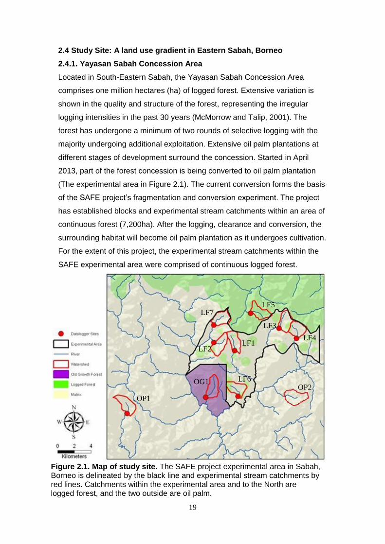
Figure 2.1. Map of study site. The SAFE project experimental area in Sabah, Borneo is delineated by the black line and experimental stream catchments by red lines. Catchments within the experimental area and to the North are logged forest, and the two outside are oil palm.

OP1

LF3

LF2 LF1

OG1 OP2

LF7

LF6

LF5

LF4

20

2.4.2 Virgin Jungle Reserve (VJR)

The Brantian Tantulit VJR is located adjacent to the South-East corner of the

experimental area (Figure 2.1). VJRs are areas of old growth forest that have

been protected and are intended for research and conservation by the Sabah

Forest Department (http://www.parks.it/world/MY/Eindex.html). This reserve

has been established as a control for old growth forest and has a stream

catchment matched in area and slope, to those in the SAFE project

experimental area (Ewers et al., 2011).

2.4.3 Benta Wawasan Oil Palm Plantation

Similarly, adjacent to the Yayasan Sabah Concession Area, is the Benta

Wawasan oil palm plantation that covers 45,601ha over 10 estates with oil

palm varying in age (http://www.bentawawasan.com.my). The estates of

Selangan Batu (South-West) and Merbau (South-East) have become

established as control sites for oil palm catchments within the SAFE project

framework.

21

3. METHODS

3.1 Framework

This project uses CMR to determine the abundance of freshwater fish species

across the land use gradient provided by the SAFE project, ranging from old

growth and logged forest to oil palm plantation. Dispersal rates of freshwater

fish at the VJR were investigated to determine if CMR would provide sufficient

recapture rates across a 200m transect. Capture histories for three focal

species were subsequently created from trapping sessions at eight

experimental streams. This data was compiled with measures of land use

(stream characteristics and riparian vegetation quality), within linear models to

evaluate how abundance varies across streams at the species level. CMR

data was also utilised to critically assess the use of trapping methodologies for

the three focal species across the land use gradient. At the community level,

multivariate ordination and absolute species turnover rates were calculated to

determine community similarity and how communities have changed over two

years.

3.2 Data Collection

3.2.1 Project design and location

The SAFE project catchments have approximately equal area and slope.

Catchments contain headstreams which are typically 2-3m wide, 2km long

and enclosed by the forest canopy (Ewers et al., 2011). Sampling was

conducted at five SAFE project streams (logged forest: LF1-5) and three other

streams outside the experimental area, chosen to match experimental

catchments in size and slope, between April – June 2013. The other streams

consisted of one in the VJR which is considered as old growth (OG1) forest,

and two in palm oil plantations (OP1 and OP2). Sampling transects, 200m in

length, were located within 100m of an in stream data logger for all streams

except OP2 that does not have a data logger (data loggers are not directly

adjacent to transects as they were installed after transects were established).

The Function of the data logger is described below (Stream variables) and the

location of all streams and data loggers can be seen in Figure 2.1.

22

3.2.2 Trapping

Fish were trapped using two methodologies, bottle trapping and cast netting,

at all experimental streams. These methods were based on previous

experimental trapping of fish at the SAFE project, September – November

2011, streams: LF1-7, OG1 and OP1. If possible, all streams were sampled

for 6 consecutive days in order to obtain accurate recapture data to model

population abundance. Due to time constraints on fieldwork and public

holidays in Malaysia during the study period, LF5 and OP1 were sampled for

5 days and LF3 was sampled for 4 days, totalling 720 trap nights for bottle

traps and 1009 cast nets were thrown. Sampling always started at the 0m

point at the downstream end of the transect, moved upstream and cast netting

was completed prior to the setting or checking of bottle traps (except on the

first day of sampling, as the 200m transect had to be marked out), providing

minimum disturbance to fish.

Bottle traps, made from recycled, plastic Blue Sky water bottles (Figure 3.1a),

were set every 10m along the 200m transect, starting at the 10m point. Traps

were placed facing upstream where possible and flush with the stream bed.

Bread and fish were used to bait alternate traps, and traps were set at each of

the experimental streams for five consecutive days. Traps were monitored

every 24 hours; fish were removed and held in containers before release. The

trap was re-baited and re-set in the same location. In the event of a flood in

the previous 24 hours, causing traps to be lost, new traps were baited and set.

In addition, fish were caught every morning of the six trapping days using a 9

foot cast net, with ¼ inch holes. Between 15-25 throws of the cast net were

made along the 200m transect at each experimental stream, with the exact

number determined by the number of pools appropriate for its use along the

transect (Figure 3.1b). Fish were removed from the net by hand and held in

containers prior to release. All fish captured were identified to genus level and

to species if possible (using Inger and Kong, 2002 and a freshwater fish list by

Hoek-Hui, 2013), body length measured, tagged if possible and released at

the point of capture.

23

Figure 3.1. Fish trapping methods. a) Blue sky water bottles had the top removed and inverted to create a trap. Five holes were made in the bottom of the bottle to allow for some water flow and traps were tied to vegetation on the stream bank. b) Photo of Research Assistant, Maria, throwing a cast net at OP2 stream.

3.2.3 Tagging protocol

A pilot study was conducted (as recommended when conducting CMR studies

in order to assess each species responses to anaesthesia, trapping, tagging,

and the precision of estimated parameters (Pine et al., 2003)), with fish caught

from a non-experimental stream. Several fish of each species were killed by

an overdose of clove oil and dissected to determine an appropriate body

cavity and method in which to insert PIT tags. It was decided to exclude all

‘suckerfish’, in the genera Protomyzon, Gastromyzon and Betta because their

flattened morphology provided no obvious body cavity large enough in which

to insert the tag. All other species with a body length (nose to tail tip) of 6cm

or over were tagged, as a conservative measure of 5.5cm recommended in

Baras et al. (2000).

The use of clove oil as an anaesthetic was tested on all species to be tagged

to determine the appropriate concentration that provided sufficient

anaesthesia coupled with rapid recovery as the effects of clove oil vary with

water temperature, fish species, size of fish and actual eugenol concentration

(Blackman, 2002; Coyle et al., 2004; Dolezelova et al., 2011). A concentration

of 30mg/L of clove oil was used as time to reach anaesthesia was on average

one minute for the different species and up to three minutes for recovery. This

a) b)

24

is consistent with recommended doses in other studies (40mg/L – Bayley and

Austen (2002), and Blackman (2002); 30-120mg/L – Hajek et al. (2006)).

Not included in the pilot was the determination of survival rates because

previous studies have shown a tag-related mortality level near zero

(Ombredance et al., 1998; Baras et al., 1999 and 2000; Zydlewshi et al.,

2001). There was no need to investigate tag retention as the ‘scar’ from

inserting the tag doubled as a secondary mark on the fish.

Fish to be tagged were held in containers after capture. The fish were

transferred and placed in 5L of water containing 30mg/L of clove oil. Fish were

held until total loss of equilibrium was reached, with slow but regular opercular

rates indicating a level of surgical anaesthesia had been reached (Coyle et al.,

2004). A 3mm incision was made posterior and ventral to the pectoral fin, and

an 11 x 2mm PIT tag (Biomark®) was inserted into the abdominal cavity and

read with the aid of a portable reader. After tagging, fish were held in 5L of

water until they had recovered, gained equilibrium and were released at the

point of capture. Any fish that did not recover, or were unable to swim, were

not released. There was no evidence of tag loss or tag failure during the

project.

3.2.4 Forest quality variables in the riparian zone

Four forest quality variables were measured in the riparian zone in order to

create an index of riparian vegetation quality that reflects levels of human

disturbance and land use (Table 3.1). Riparian vegetation surrounding each

stream was assessed every 50m, for 500m upstream from the 0m point on

both banks. At each 50m point, measurements were taken approximately 10m

up the bank, or the nearest area of level ground beyond that.

25

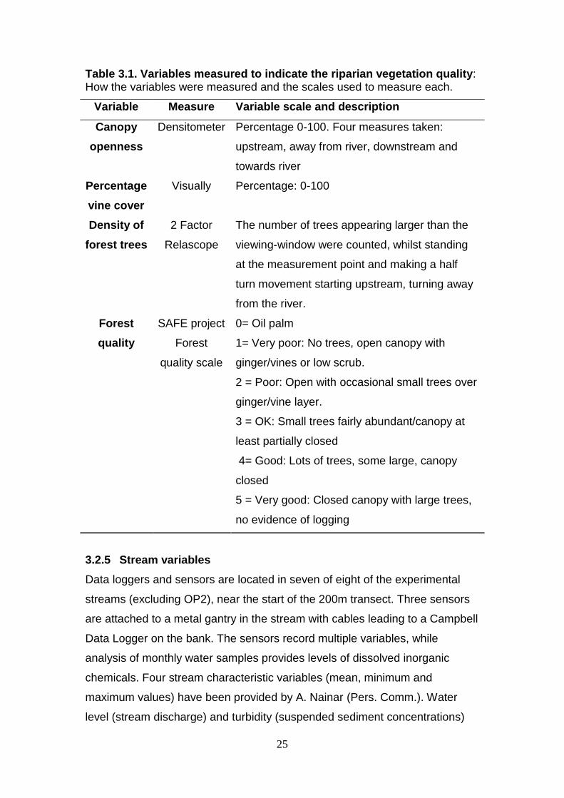
Table 3.1. Variables measured to indicate the riparian vegetation quality: How the variables were measured and the scales used to measure each.

Variable Measure Variable scale and description

Canopy

openness

Densitometer Percentage 0-100. Four measures taken:

upstream, away from river, downstream and

towards river

Percentage

vine cover

Visually Percentage: 0-100

Density of

forest trees

2 Factor

Relascope

The number of trees appearing larger than the

viewing-window were counted, whilst standing

at the measurement point and making a half

turn movement starting upstream, turning away

from the river.

Forest

quality

SAFE project

Forest

quality scale

0= Oil palm

1= Very poor: No trees, open canopy with

ginger/vines or low scrub.

2 = Poor: Open with occasional small trees over

ginger/vine layer.

3 = OK: Small trees fairly abundant/canopy at

least partially closed

4= Good: Lots of trees, some large, canopy

closed

5 = Very good: Closed canopy with large trees,

no evidence of logging

3.2.5 Stream variables

Data loggers and sensors are located in seven of eight of the experimental

streams (excluding OP2), near the start of the 200m transect. Three sensors

are attached to a metal gantry in the stream with cables leading to a Campbell

Data Logger on the bank. The sensors record multiple variables, while

analysis of monthly water samples provides levels of dissolved inorganic

chemicals. Four stream characteristic variables (mean, minimum and

maximum values) have been provided by A. Nainar (Pers. Comm.). Water

level (stream discharge) and turbidity (suspended sediment concentrations)

26

are measured every five minutes by the in stream sensors. Nitrate and

phosphorus concentrations are obtained from analysed monthly water

samples. These four measures are indicators of stream characteristics; and

provide insight into the catchment allochthonous inputs to streams, allowing

for comparisons across the land use gradient.

3.3 Data analyses

3.3.1 Dispersal

The distance travelled by fish indicates the rate and extent of dispersal, which

could justify the use of mark-recapture to study fish over a 200m transect or

prove that 200m is not an adequate distance. This data could also be

essential information if attempting to protect endangered or protected fish or

pescivorous species. OG1 was intensively re-sampled for three days, four

weeks after the first 6 days of sampling. Bottle traps were set every 10m, and

55-60 cast nets thrown along a 600m transect (the experimental transect at

200-400m). Distance since last capture was calculated for each recaptured

individual of the three focal species and plotted on histograms to compare

dispersal rates. The null distribution was calculated from the probability of

being able to be recaptured at each sampling point.

3.3.2 Abundance estimation

The two most common species and one genus (Nematobramis everetti, Tor

dourensis and the genus Rasbora) were modelled using the programme

MARK (White and Burnham, 1999) to obtain population size (N) estimates for

each stream they were present in. These species and genus were chosen due

to sufficient recapture data, and the genera grouped to prevent any mis-

identification. Only streams providing recapture rates could be considered for

modelling. Data input consisted of capture histories, compiled from both bottle

trap and cast netting methods, detailing the unique ID of successive captures

for each individual. Capture histories were input into the programme MARK

and population estimates derived using the POPAN formulation of Jolly Seber

models (Jolly, 1965; Seber, 1965) for live encounters and recaptures, using

the variables: p, phi, b and t.

27

A fully time dependant model was first used to model the data (Table 3.2) as it

consisted of the greatest number of parameters and was therefore tested for

goodness of fit using RELEASE, a programme run within MARK. RELEASE

uses data (in the form of live recaptures) to calculate a c-hat score, which

measures the goodness of fit of the models and degree of dispersion of the

data (Cooch and White, 2012). The results of tests 2 and 3 from RELEASE

enabled the c-hat score to be calculated (c-hat = ∑X2/∑df) and the models

could then be adjusted to account for dispersion of the data (Cooch and

White, 2012). Due to low recapture rates and low captures for some species

and/or locations, several RELEASE goodness of fit tests were unable to be

performed due to ‘insufficient data’. Populations for each species were

grouped and the test re-run to give a c-hat value applicable to each species.

C-hat values were greater than one for Rasbora (1.524) and N. everetti

(1.307) and were adjusted accordingly in Mark to account for over-dispersion

in the data. A C-hat value of one was maintained for T. dourensis as the c-hat

value was less than one (0.486), as there is no consensus within the literature

to estimate under-dispersion of data (Cooch and White, 2012).

Additional models were run, varying time dependence of each or all

parameters, by manipulation of the PIM charts (Table 3.2). The parm-specific

link function was specified in the run menu, and in the design matrix: Sin for p

and phi parameters, MLogit(1) for all b parameters as they need to sum to 1,

and Log for N, the population parameter (Schwarz and Arnason, 2012).

Models were compared using AIC values; the model with the lowest AIC is the

most parsimonious and thus considered the closest to the ‘true’ scenario.

Models were averaged to calculate a population estimate; accounting for all

variation in the models, by taking a weighted average according to the models

corrected AIC (AICc) weight and model likelihood. Models were averaged

using real values, to calculate the initial population size, N, for each population

that could be modelled for the three focal species. If no recapture data was

available for the three focal species, the number of unique individuals was

used as a measure of minimum population size.

28

Table 3.2. Models used to estimate abundance of Rasbora, N. everetti and T. dourensis in the programme mark. The variables in the models are: p – the probability of capture of marked and unmarked individuals, phi – the survival probability of marked and unmarked individuals, b – the probability of individuals entering the modelled area and t – time.

Model Description

p(t), phi(t), b(t)

p(.), phi(t), b(t)

p(.), phi(.), b(t)

p(t), phi(.), b(t)

Time dependant catchability and survival

Constant catchability over time and time dependant

survival.

Constant survival and catchability over time.

Constant survival over time and time dependant

catchability.

3.3.3 Comparison of abundance across the land use gradient

Principle component analysis (PCA) was performed (as was all analysis in the

statistical programme, R (R Development team, 2013)) on four variables of

riparian vegetation quality and four variables of stream characteristics

providing two indices across the land use gradient. To determine if the indices

of land use effectively split up streams by land use, mixed effects models (with

and without the fixed effect) were run on the Principle Component 1 (PC1)

values (as a function of land use (fixed) effect and stream (random) effect).

ANOVA was then conducted to determine if land use had a significant effect,

indicating that the indices represent the land use gradient. Correlation was

tested between riparian vegetation and stream characteristics to determine

that they were different, even though they are not independent.

Poisson’s Generalised Linear Models (GLMs) were performed for each focal

species population abundance estimates to determine which variables (PC1

riparian vegetation, PC1 stream characteristics and/or Land use) predicted the

data. Poisson’s GLMs were used as the outcome variable (abundance) is

count data, with a set of continuous predictor variables. GLMs were run,

starting with the most parameterised model (Abundance estimate ~ PC1value

of riparian vegetation x Land use x PC1 value of streams) and undergoing

model simplification. The stream OP2, was removed from analysis as no data

logger is present in the stream, resulting in no stream characteristics data.

29

The AIC value of the models was compared to that of the null model (~1) and

ANOVA was conducted to determine if there was a significant difference to

the null model.

3.3.4 Methodological comparison

Mixed effects models of standardised catch data (per trap, per day), with the

abundance estimate from MARK as the fixed effect and stream as random the

random effect were run. They were used to determine which trapping method,

bottle traps or cast netting, was most appropriate in predicting the abundance

of the three focal species. ANOVA was used to test the significance of models

against the null model. The chi-squared value and slope of the model were

used to compare the predictive power of models.

3.3.5 Community level comparisons across the land use gradient

Multivariate ordination (Principle Co-ordinates Analysis (PCoA) using the Bray

distance function) in the vegan package of R (Oksanen et al., 2013), was

used to test the similarity between species and streams. A site-by-species

matrix was created utilising catch data from this sampling season and from a

previous sampling season, September - December 2011. Both indices of land

use were fit to the analysis indicating the direction of greatest change.

MANOVA tests were run, to determine the effect of year, land use and the

interaction on the Axis’s co-ordinates of each stream to test for a temporal

difference and/or land use effect. ANOVA were subsequently run to test the

effects of year and land use on relative abundance of two genera, Rasbora

and Tor (grouped to account for identification issues), and three species (N.

everetti, Protomyzon griswoldi and Systomus sealei) all of which were distinct

in the PCoA analysis.

Absolute species turnover rates (β, as a measure of beta diversity) could also

be calculated across the land use gradient between the two sampling years

indicating the change in species composition over time. β = (s1 – c) + (s2 – c),

where s1 = total number of species in first community, s2 = total number of

species in second community and c = number of species in both communities.

30

GLMs were fitted of absolute turnover rates across the land use gradient

indices of riparian vegetation quality and stream characteristics.

31

Figure 4.1. Dispersal of fish from all and the three focal species/genus. Dispersal is measured by the distance (metres) moved by the fish since the last capture, for a) all fish, b) N. everetti c) T. dourensis d) Rasbora. The red line illustrates the expected distribution of fish movement, calculated from the probability of moving each distance from known trapping points in the 600m transect.

4. RESULTS

4.1 Fish Dispersal

Dispersal varied from 0 – 300m for all the fish that were recaptured from the

three focal species at the OG1 stream (Figure 4.1). T. dourensis moved the

least distance, but all fish tended to stay in the same locality over the study

period, with 89% of fish recaptured less than 20m from the point of last

capture. This is despite environmental conditions varying over the project

duration, including regular flood events after periods of heavy rainfall. The

lack of dispersal indicates that a mark-recapture study will be appropriate for

fish in these headstreams and that a 200m transect is a sufficient size to

capture a ‘snapshot’ of species abundance.

32

4.2 Indices of land use gradient

For both indices, the PCA found a gradient across the land uses, from OG

(negative numbers) to OP (positive numbers) with LF ranging between the

two. However, the differences between the land uses was much smaller

between OG and LF, than OP. ANOVA of mixed effects models of the riparian

vegetation PC1 values, showed that the index of riparian vegetation effectively

separated oil palm streams (Figure 4.2) from logged forest and old growth

(p=0.027, chisq=7.188, df=2). The index of stream characteristics was also

shown to effectively split up stream PC1 values in ANOVA tests of mixed

effects models (p<0.001, chisq=21.559 df=2). However, the tests were

inconclusive as there are only single values available for each stream and

only one replicate of each OG and OP, providing little variation.

Correlation between the two indices was tested to determine the relationship

between the land use variables. A weak positive correlation (r=0.283) was

indicated as expected, but there was no significant correlation between the

two variables (p=0.539, t=0.659, df=5), indicating responses to land use will

be different for the two indices.

Figure 4.2. PCA of riparian vegetation variables effectively splits streams up into different land uses. Two models: PC1 values riparian vegetation index as a function of land use (fixed) effect and stream (random) and a null model excluding the fixed effect, were significantly different in an ANOVA test p = 0.02749 (chisq= 7.188, df= 2).

33

4.3 Population modelling and estimation

Only one stream had caught individuals of a focal species with insufficient

data to calculate abundance. Three T. dourensis were caught at OP2 and this

number was used as a minimum abundance estimate since abundance could

not be modelled. Zeros indicate that individuals of the focal species/genus

were not found.

Population abundance has large variation across streams for the three focal

taxa (Table 4.1). The largest population modelled was N. everetti at OP2 and

no fish of the three focal taxa were caught at two streams (OP1 and LF2).

Despite this, the three focal taxa were present at all three land uses and

subsequent models will explore the relationship of abundance across land

use. The large standard errors for abundance estimations, is mainly due to

low capture and recapture rates, but also the altered c-hat values for Rasbora

and N. everetti indicating the level of over-dispersion in the data.

The model of best fit varied by species and stream, for 50% of estimates p(.),

phi(.), b(t) was the best fit to the data. This model indicated a constant

catchability and survival over time, suggesting that all assumptions of mark

recapture modelling were satisfied. The best model for 25% of estimates was

p(.),phi(t),b(t) indicating that survival was time dependant, but the assumption

of equal survival of marked and unmarked animals at each sampling occasion

is still met. The best model for the remaining 25% of estimates was

p(t),phi(.),b(t) suggesting catchability varied between sampling occasions but

the assumption of equal catchability of all animals at each sampling occasion

is still met. The variation in catchability in sampling occasions may be related

to water levels that subsequently reflect weather conditions and flood events.

34

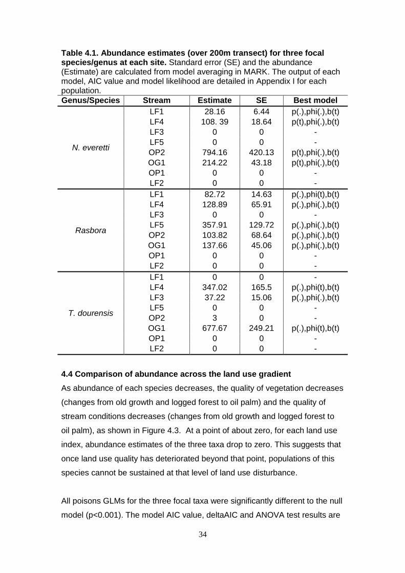
Table 4.1. Abundance estimates (over 200m transect) for three focal species/genus at each site. Standard error (SE) and the abundance (Estimate) are calculated from model averaging in MARK. The output of each model, AIC value and model likelihood are detailed in Appendix I for each population.

Genus/Species Stream Estimate SE Best model

N. everetti

LF1 28.16 6.44 p(.),phi(.),b(t)

LF4 108. 39 18.64 p(t),phi(.),b(t)

LF3 0 0 -

LF5 0 0 -

OP2 794.16 420.13 p(t),phi(.),b(t)

OG1 214.22 43.18 p(t),phi(.),b(t)

OP1 0 0 -

LF2 0 0 -

Rasbora

LF1 82.72 14.63 p(.),phi(t),b(t)

LF4 128.89 65.91 p(.),phi(.),b(t)

LF3 0 0 -

LF5 357.91 129.72 p(.),phi(.),b(t)

OP2 103.82 68.64 p(.),phi(.),b(t)

OG1 137.66 45.06 p(.),phi(.),b(t)

OP1 0 0 -

LF2 0 0 -

T. dourensis

LF1 0 0 -

LF4 347.02 165.5 p(.),phi(t),b(t)

LF3 37.22 15.06 p(.),phi(.),b(t)

LF5 0 0 -

OP2 3 0 -

OG1 677.67 249.21 p(.),phi(t),b(t)

OP1 0 0 -

LF2 0 0 -

4.4 Comparison of abundance across the land use gradient

As abundance of each species decreases, the quality of vegetation decreases

(changes from old growth and logged forest to oil palm) and the quality of

stream conditions decreases (changes from old growth and logged forest to

oil palm), as shown in Figure 4.3. At a point of about zero, for each land use

index, abundance estimates of the three taxa drop to zero. This suggests that

once land use quality has deteriorated beyond that point, populations of this

species cannot be sustained at that level of land use disturbance.

All poisons GLMs for the three focal taxa were significantly different to the null

model (p<0.001). The model AIC value, deltaAIC and ANOVA test results are

35

in Appendix II. The AIC values demonstrated that the model: Abundance

estimate ~ PC1value of riparian vegetation x Land use + PC1 value of stream

characteristics was most significant for N. everetti and T. dourensis. The

model indicated that as the vegetation quality increases along the index

gradient (OG to OP) the amount the abundance decreases is dependent upon

the land use. However, the lack of data points for OG and OP prevent

interpretation of land use interaction. There was no interaction with the PC1 of

stream characteristics indicating that stream characteristics influences

abundance in a linear relationship but is not influenced by the PC1 value of

riparian vegetation or land-use.

In comparison, the most parameterised model (Abundance estimate ~

PC1value of riparian vegetation x Land use x PC1 value of stream

characteristics) had the lowest AIC value for Rasbora. The model shows that

as the vegetation quality increases (OG to OP) along the index gradient and

stream quality increases (OG to OP) along the index gradient, the abundance

decreases with respect to land use (as above, only the LF interaction can be

explored). This interaction or inclusion of all response variables in the models

was expected, as the variables are not independent and all influence the

environment the fish inhabit.

36

.

Figure 4.3. Modelled abundance against indices of riparian vegetation and stream quality, for three focal species. Points labelled by land use; black line indicates the glm Abundance ~ PC1 riparian vegetation and Abundance ~ PC1 stream characteristics and the red lines are the 95% confidence intervals to this model. Riparian vegetation index values are the axis one scores from a PCA of canopy openness, relascope count, percentage vine cover and the SAFE project forest quality scale, and reflect a gradient from high quality (negative values) to low quality (positive values) vegetation. Stream quality index values are the axis one scores from a PCA of water level, turbidity, nitrate concentration and phosphorous concentration, and reflect the same gradient for stream characteristics.

37

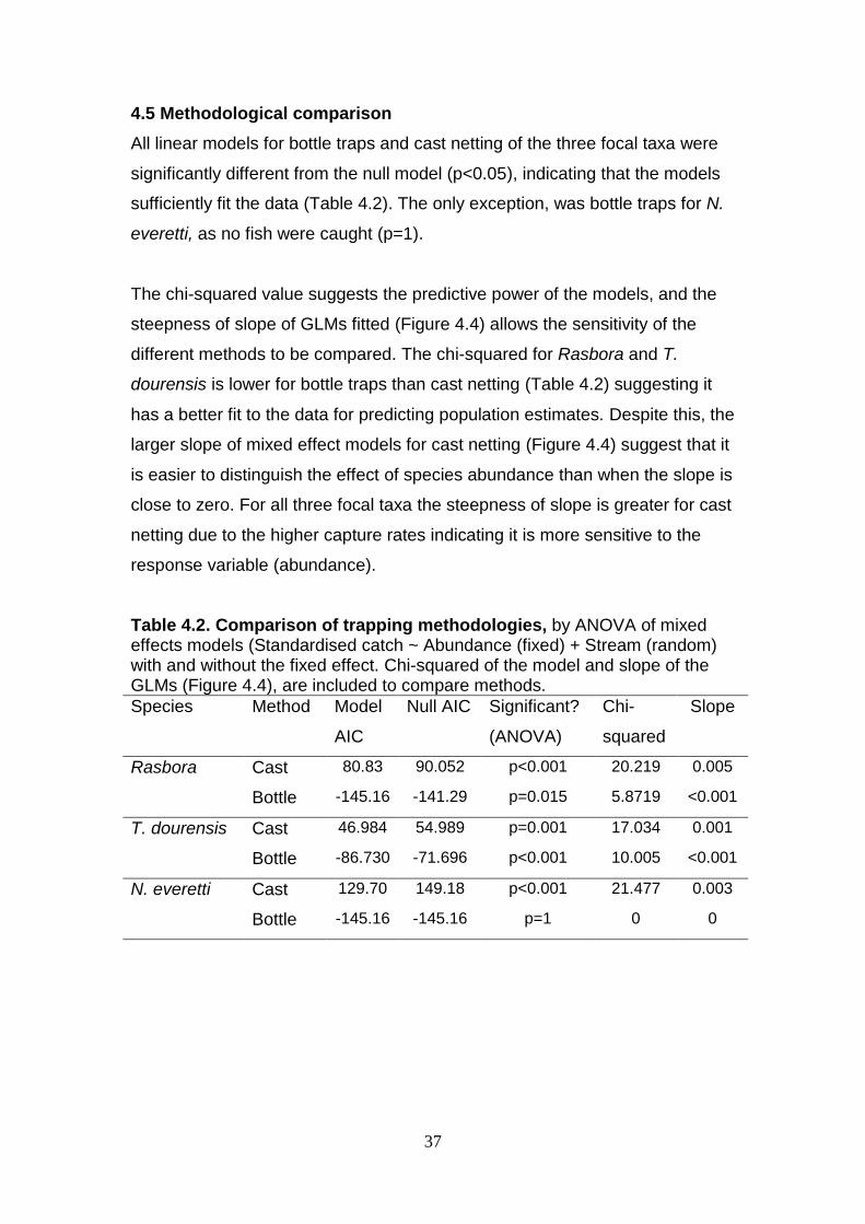
4.5 Methodological comparison

All linear models for bottle traps and cast netting of the three focal taxa were

significantly different from the null model (p<0.05), indicating that the models

sufficiently fit the data (Table 4.2). The only exception, was bottle traps for N.

everetti, as no fish were caught (p=1).

The chi-squared value suggests the predictive power of the models, and the

steepness of slope of GLMs fitted (Figure 4.4) allows the sensitivity of the

different methods to be compared. The chi-squared for Rasbora and T.

dourensis is lower for bottle traps than cast netting (Table 4.2) suggesting it

has a better fit to the data for predicting population estimates. Despite this, the

larger slope of mixed effect models for cast netting (Figure 4.4) suggest that it

is easier to distinguish the effect of species abundance than when the slope is

close to zero. For all three focal taxa the steepness of slope is greater for cast

netting due to the higher capture rates indicating it is more sensitive to the

response variable (abundance).

Table 4.2. Comparison of trapping methodologies, by ANOVA of mixed effects models (Standardised catch ~ Abundance (fixed) + Stream (random) with and without the fixed effect. Chi-squared of the model and slope of the GLMs (Figure 4.4), are included to compare methods.

Species Method Model

AIC

Null AIC Significant?

(ANOVA)

Chi-

squared

Slope

Rasbora Cast 80.83 90.052 p<0.001 20.219 0.005

Bottle -145.16 -141.29 p=0.015 5.8719 <0.001

T. dourensis Cast 46.984 54.989 p=0.001 17.034 0.001

Bottle -86.730 -71.696 p<0.001 10.005 <0.001

N. everetti Cast 129.70 149.18 p<0.001 21.477 0.003

Bottle -145.16 -145.16 p=1 0 0

38

Figure 4.4. Comparison of trapping methods, bottle trapping and cast netting, for the three focal taxa. Methods are standardised to per trap per day (blue = cast netting, red = bottle traps). GLMs (catch ~ abundance) have been fit to the graph, as mixed effects models (used for analysis) cannot be predicted as the random effect value is unknown.

39

4.6 Community similarity and turnover rates

The most recent sampling in 2013 saw a total of 2779 fish captures from 11

genera, totalling 14 different species and the genus Rasbora which was not

identified to species level. The 2011 sampling season saw a total of 2345 fish

captures, of 19 different species in 12 genera. This disparity suggests some

difference of community composition between sampling seasons.

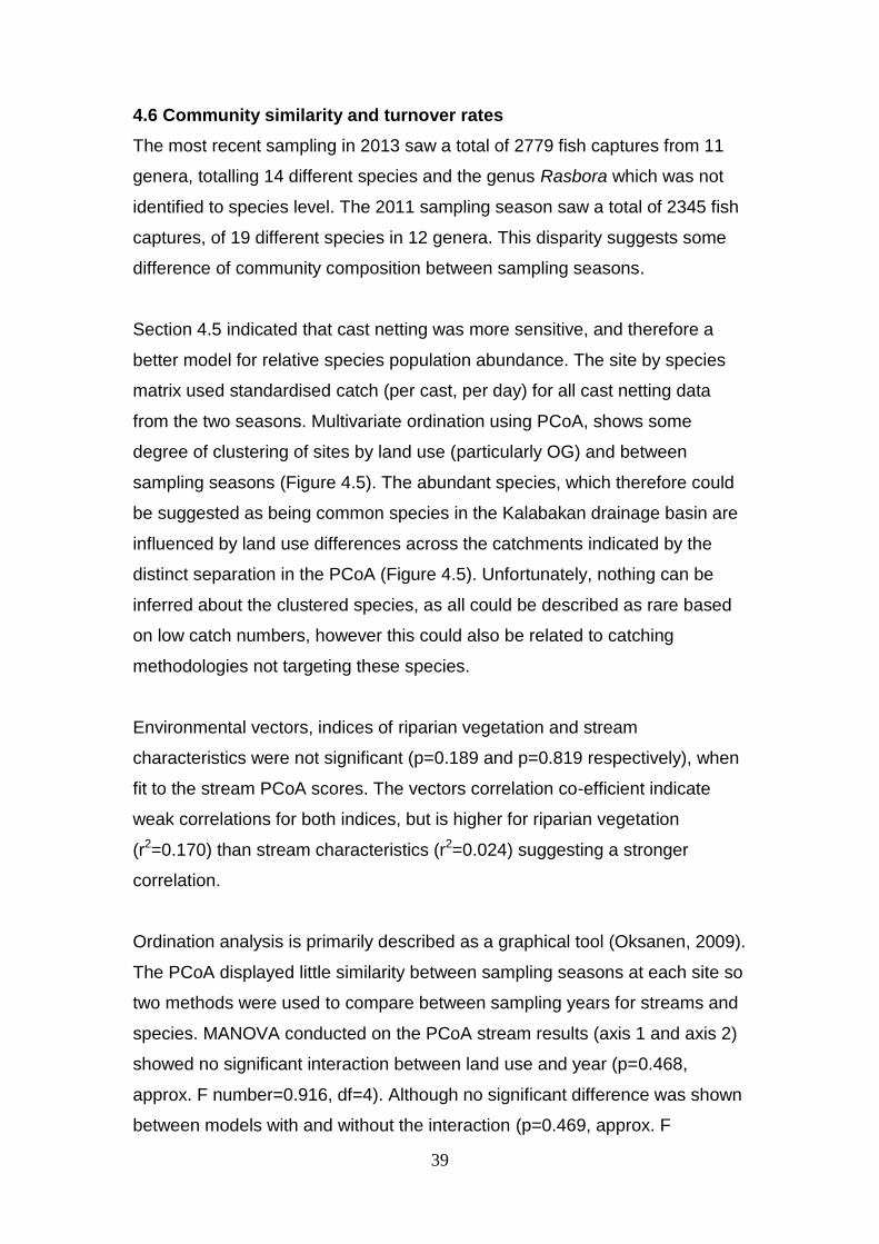
Section 4.5 indicated that cast netting was more sensitive, and therefore a

better model for relative species population abundance. The site by species

matrix used standardised catch (per cast, per day) for all cast netting data

from the two seasons. Multivariate ordination using PCoA, shows some

degree of clustering of sites by land use (particularly OG) and between

sampling seasons (Figure 4.5). The abundant species, which therefore could

be suggested as being common species in the Kalabakan drainage basin are

influenced by land use differences across the catchments indicated by the

distinct separation in the PCoA (Figure 4.5). Unfortunately, nothing can be

inferred about the clustered species, as all could be described as rare based

on low catch numbers, however this could also be related to catching

methodologies not targeting these species.

Environmental vectors, indices of riparian vegetation and stream

characteristics were not significant (p=0.189 and p=0.819 respectively), when

fit to the stream PCoA scores. The vectors correlation co-efficient indicate

weak correlations for both indices, but is higher for riparian vegetation

(r2=0.170) than stream characteristics (r2=0.024) suggesting a stronger

correlation.

Ordination analysis is primarily described as a graphical tool (Oksanen, 2009).

The PCoA displayed little similarity between sampling seasons at each site so

two methods were used to compare between sampling years for streams and

species. MANOVA conducted on the PCoA stream results (axis 1 and axis 2)

showed no significant interaction between land use and year (p=0.468,

approx. F number=0.916, df=4). Although no significant difference was shown

between models with and without the interaction (p=0.469, approx. F

40

number=0.91562, df=4), therefore the interaction was removed from the

analysis. Subsequently, MANOVA conducted on the PCoA stream results

suggested that there is a slight, albeit non-significant difference between

sampling years (p=0.054, approx. F number=3.571, df=2) and land use

(p=0.098, approx. F number=2.1441, df=4) for predicting the similarity

distance between sites.

Tor Rasbora

P. griswoldi

S. sealei

N. everetti

Figure 4.5. Multivariate ordination using PCoA, for two sampling seasons across all experimental streams. Stream and sampling date (black) and species or genus (red) are displayed along the first two axis’s of the analysis. Blue arrows indicate direction of most rapid change for the two environmental indices: stream characteristics (StreamPCA) and riparian vegetation (vegetationPCA). All species names that can be read are abundant species (including the three focal species and others caught at most locations), all others are clustered around 0, 0 and are considered as less abundant.

41

Results of ANOVA of relative abundance by year and land use varied for each

species or genus as all have different biological requirements (for example

food and substrate). Relative abundance of S. sealei decreased from, 2011 to

2013 (p=0.005, F=10.631, df=1), increased from OG to OP (p=0.038,

F=4.047, df=2), but proportionately to land use, with the greatest decrease in

OP and smallest in OG (p=0.008, F=6.591, df=2). No significance for year or

land use (p>0.05) was shown for the other four taxa, although this may be due

to small sample sizes for OG and OP.

Relative abundance, indicated by standardised catch (per cast, per day),

varied by year and land use (Appendix III). Tor and Rasbora had the largest

populations in OG and lowest in OP, whereas the opposite was true for P.

griswoldi and N. everetti. The effect of year was similar, with no clear

difference for Tor and Rasbora, more caught in 2013 for P. griswoldi and more

caught in 2011 for N. everetti. The difference between species response

suggests that the effects of land use and sampling year cannot predict the

community effect as different species can adapt to or may be resilient to

different conditions.

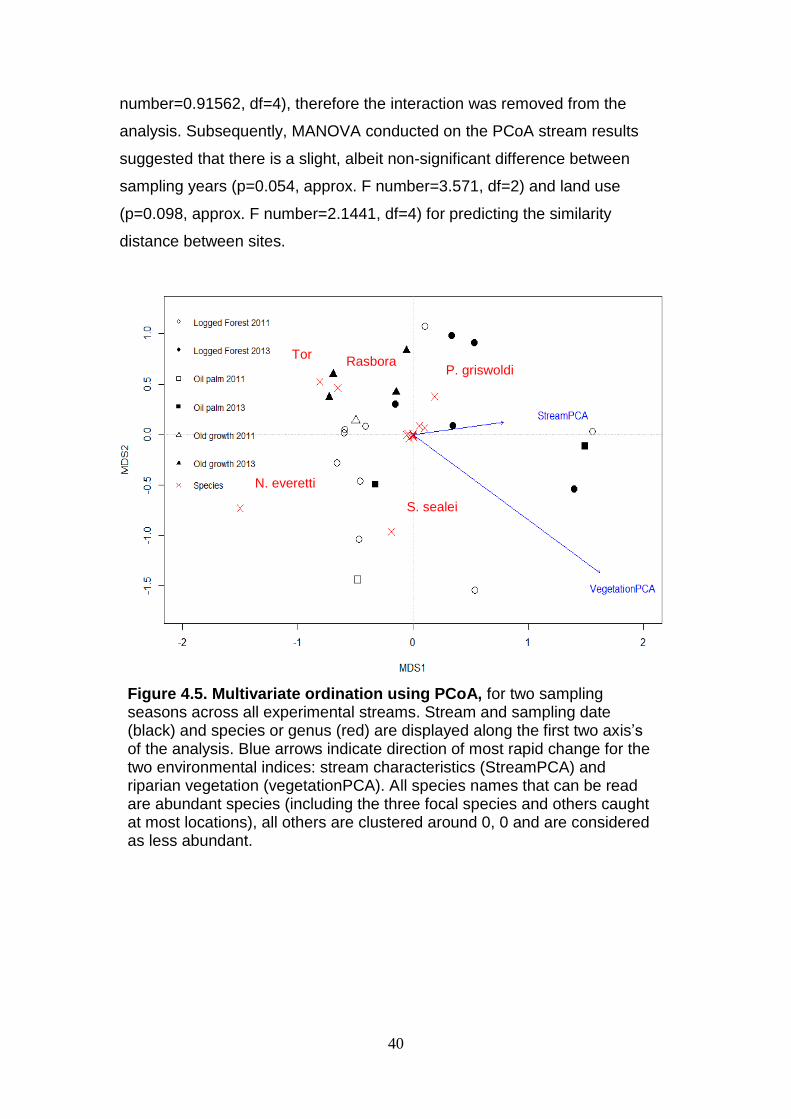
Absolute species turnover rates indicating how stream communities have

changed between seasons (Figure 4.6), were calculated for the seven

streams sampled in both seasons (LF1-5, OG1 and OP1). Species turnover

rates increase as riparian vegetation quality decreases, changes from OG/LF

to OP, although it is not significant (p=0.338), and less than AIC two units

separate experimental (39.1) and null (38.28) models. Species turnover rates

decrease as stream characteristics change from OG/LF streams to that of OP

although it is not significant (p=0.869), and less than two AIC units separate

experimental (40.24) and null (38.28) models. The result concludes that

species turnover rates vary between streams, but the reasoning cannot be

confirmed.

42

Figure 4.6. Absolute species turnover rates against indices of land use, riparian vegetation (left) and stream characteristics (right). Points are labelled by land use and where possible standard error bars fit. Riparian vegetation index values are the axis one scores from a PCA of canopy openness, relascope count, percentage vine cover and the SAFE project forest quality scale, and reflect a gradient from high quality (negative values) to low quality (positive values) vegetation. Stream quality index values are the axis one scores from a PCA of water level, turbidity, nitrate concentration and phosphorous concentration, and reflect a gradient from high quality (negative values) to low quality (positive values) stream conditions.

43

5. DISCUSSION

5.1 Response of fish to logging and conversion to oil palm

5.1.1 Species level

This project illustrates that fish species have varying responses to logging and

conversion to oil palm. Abundance estimates of the three focal, common taxa

decreased across the land use gradient (from old growth and logged forest to

oil palm) for both riparian vegetation and stream characteristics. Tor and

Rasbora had the largest populations in old growth forest whereas the largest

populations for P. griswoldi and N. everetti were in oil palm. The value of

logged forest and oil palm catchments is evident from the results in this

project, as shown by the wide variety in abundance estimates for streams in

the different land use areas.

The paucity of studies on tropical freshwater fish makes comparison to other

areas difficult. Most studies focus on community assemblages and diversity

rather than abundance, as was done in this work. Martin-Smith and Tan

(1998b) recorded 65 different species of fish in DVCA, the Lower Segama and

Upper Kuamut Rivers. However, Martin-Smith and Laird (1998) recorded that

up to 30 species of fish were generally found in medium-sized rainforest

streams across the land use gradient in Sabah. Currently, a total of only 20

species from 5 families have been recorded from the SAFE project area,

although streams are narrow headstreams. This is in line with Martin-Smiths

studies as more species can be expected, once more thorough surveys are

conducted (Hoek-Hui, 2013).

The effects of logging vary widely, but depend upon the extent of logging in

the region, the distribution of commercially valuable trees, and the local

topography (Martin-Smith, 1998b). Typically, selective logging involves the

removal of trees over 60 cm diameter at breast height (DBH). The act of

logging and resultant skidding operations, to remove trees, can kill 30-50% of

trees that are 1-60cm DBH (Pinard and Putz, 1996). In addition, the logging

roads and skid marks created with logging activity have no designed drainage

systems. Sidle et al. (2004) demonstrated how 78% of soil loss from the road

44

system was delivered to a small headwater catchment, in Peninsular

Malaysia. Once in the stream, much of the sediment was temporarily stored

behind fallen woody debris, increasing the stream sediment load (Sidle et al.,

2004). This additional degradation exacerbates the problems of logging in the

region, but it is the type and extent of logging practices that affect fish diversity

and abundance.

Martin-Smith (1998a) demonstrated that there was little difference between

abundance of species in old growth or logged forest, but there was a

difference in abundance and biomass for three fish species in streams that

had been recently logged (3-7 years) and old logged (17-18 years). The focal

species of this project are different to those studied by Martin-Smith and the

diversity of species at the SAFE project is considerably lower than that of

DVCA. In this project logging occurred at all logged forest catchments in the

1970’s and again between 2001-2008, whilst oil palm was planted in 2000 to

2006, dependent upon the estate (Ewers et al., 2011), similar time periods to

Martin-Smiths studies. A distinction across the logging gradient was indicated,

but it is worth noting that the three focal species were not recorded at all

streams, with differences across the LF streams. This indicates fish diversity

and abundance is influenced by additional habitat level factors

Studies by Martin-Smith suggest logging does not affect species abundance

or diversity over the long term, but this is confined to one region in Sabah.

Further studies are needed to quantify the effects of logging on freshwater

biota in a wider geographical context.

The effect of conversion to oil palm cannot be inferred from this project, only

suggestions about post-conversion to oil palm can be discussed. The results

of this project demonstrate that fish species can survive in streams within oil

palm catchments, but abundance and species distribution is varied. One oil

palm stream had the greatest abundance of a focal species and had the

second highest level of diversity. The second oil palm stream had much lower

species diversity and no recapture data was available due to very low catches

or no catches of the focal species were caught. Unfortunately, the stream with

45

higher catch was excluded from the majority of analysis as no in-stream data

logger was present, resulting in little inference from the high level of diversity.

The two oil palm streams differ as one has a narrow forest riparian strip along

the majority of the experimental catchment compared to no riparian strip at the

other (Pers. Obs).

Current environmental legislation in Malaysia states that a 30m buffer strip is

left on either side of streams with permanent water flows (Ewers et al., 2011).

However, previous logging practices and conversion to oil palm often did not

adhere to this, and there is no confirmation that 30m is sufficient to protect

biodiversity and ecosystem services provided by headstreams. The future

direction, to manipulate widths of experimental riparian strips (0–120m), at the

SAFE project catchments will determine the short and long term effects of

logging and conversion to oil palm (Ewers et al., 2011). The results provided

by this large scale experiment at the SAFE project will demonstrate how fish

species are affected by logging disturbance, forest clearance, and eventual

conversion to oil palm plantation over time. As deforestation is going to

continue into the future, results of this work will identify what width of riparian

strip is optimal in maintaining freshwater diversity and abundance in Sabah.

5.1.2 Community level

Community composition varied across the land use gradient of the SAFE

project. Results indicated decreased abundance and diversity as vegetation

and stream quality decreased (old growth and logged forest to oil palm).

There is a dearth of empirical evidence supporting the role of retained riparian

forests in the maintenance of tropical fish assemblages (Dudgeon, 2000;

Iwato et al., 2005; Jackson and Sweeney, 1995). Despite this, literature is

divided on the effects of logging and deforestation on tropical freshwater fish

community assemblages. The few quantitative studies conducted on the

communities and abundance of fish fauna in Sabah remains somewhat

sporadic (Martin-Smith and Hoek-Hui, 1998), but several different hypotheses

have arisen to explain the distribution and diversity of fish.

46

The removal of tropical forest cover during timber extraction represents an

extreme form of disturbance, with potentially far-reaching effects on fish

biodiversity. Martin-Smith et al. (1999) showed few long-term changes in

abundance or species composition from streams around DVCA, with a diverse

assemblage of more than 30 species of fish found in both sets of streams. As

discussed, species can be affected by the time since logging which suggests

logging has an effect on fish communities. Martin-Smith (1998b) suggested

this effect of timber extraction is subtle, with changes being shown in

abundance distributions rather than differences in community composition.

Although, some communities did display short term (<18 months) absence or

decrease in fish species after logging events.

In contrast to Martin-Smith but in agreement to this project, Inoue and

Nunakawa (2005) demonstrated that riparian forests strongly affected the fish

assemblage and abundance in low order streams. This can be explained by

the obvious benefits provided by riparian vegetation to streams, in regulating

allochthonous, sediment and light inputs to streams (Inoue and Nakano, 1998;

Inoue and Nunakawa, 2005; Tabacchi et al., 1998). Iwato et al. (2005)

demonstrated that habitat alteration (through sedimentation, highly associated

with logging and conversion of forest to palm oil) lowered the abundance

and/or diversity of every benthic assemblage. In comparison, nektonic fishes

were less affected, but the overall effects were detrimental, leading to a

reduction in biodiversity of the stream communities.

A third explanation to the distribution and abundance of fish was

demonstrated by Martin-Smith (1998a, 1998b). Martin-Smith (1998a)

suggested that mesohabitats (riffles and pools) within streams and differences

in stream size were more important in determining community structure of

tropical freshwater fish communities in Sabah than logging history. Martin-

Smith (1998a) concluded that the type of selective logging practices used

locally had little impact on fish communities through mechanisms of

persistance and rapid recolinisation. This project has not explicitly tested for

possible differences in mesohabitats and therefore cannot be directly

compared. The majority of sampling was conducted in pools, due to the

47

methods involved in fish capture, so a difference in mesohabitats is not

distinguishable. Explanations for the persistence of fish communities in the

face of high disturbance pressure include high rates of re-colonisation,

movement from undisturbed areas and avoidance or tolerance of disturbance

effects (Martin-Smith,1998b; Martin-Smith et al., 2010), proposing that

communities are highly resilient.

In addition, the reported diversity of fish species at the SAFE project is

currently considerably lower than that of DVCA. Martin-Smith and Laird (1998)

studied depauperate communities (<10 species) in the Segama River region

of Sabah. The streams either had substantial barriers to movement in the form

of waterfalls and cascades, or unrestricted access but few species (Martin-

Smith, 1998). Both of these environments compare to streams in this project,

for example small waterfalls present in three logged forest streams (Pers.

Obs). Martin-Smith and Laird (1998) showed abundance and biomass of fish

above waterfalls were significantly lower than all other sites and fish were

predominantly herbivores. Fishes in the other forest streams were from a

variety of trophic groups. Fish caught in this project encompass all trophic

levels but varied across the land use gradient. Food availability provides a

possible explanation for the difference in abundance and community

composition, both at the SAFE project and at the wider geographic scale.

Further work should be conducted to confirm this assumption, to enable

implications for management and future conservation efforts.

Shifting the focus to temperate freshwater fish, Inoue and Nunakawa (2005)

demonstrated that substrate heterogeneity and competitor abundance were

the most important variables in determining population abundance of two

benthic species in Japanese streams. Riparian vegetation had no effect on

food availability that limited fish populations, whereas this study showed that

land use indices were a significant variable in estimating population

abundance. In addition, a review of temperate stream-fish community studies

concluded that stream and river fish communities were not resilient to logging

in the absence of mitigation effects (Detenbeck et al.,1992). This is in contrast

48

to what is seen in tropical freshwater fish communities (Martin-Smith, 1998b;

Martin-Smith et al., 1999).

The results also demonstrated diversity of species was influenced by

sampling season. The confirmation of difference between sampling years and

the lack of corroboration between species turnover rates across the land use

indices could be explained by a number of factors, none of which can be

confirmed within this study. This difference could relate to actual differences in

community structure and/or diversity, the ability of research assistants

employed to catch fish using a cast net, correct identification of species

(although as far as possible this was controlled for by grouping species to

genera for Tor and Rasbora), and the sampling duration at each stream

(where possible this project sampled a stream for 6 consecutive days, in 2011

sampling was more random). This necessitates the cautious treatment of

results and the inferences that can be drawn, but does not influence how the

diversity varies across the land use gradient focused on in the project, as it is

indicated in both years.

5.2 Dispersal

This project showed fish in headstreams are highly sedentary, which was an

advantage to the project as it enabled fish to be re-caught across a 200m

transect. This is expected as the streams sampled are steep and fast flowing,

with many small waterfalls and drops. Streams are impassable in low water

and a raging torrent in high water (Pers. Obs). As previously stated, Martin-

Smith (1998a) suggested fish are specific to mesohabitats, confining them to

these localities within streams. Martin-Smith (2010) suggested depauperate

communities were present above waterfalls, a significant barrier to migration,

preventing dispersal, although this project did not have the scope to confirm if

this was the cause of limited dispersal.

5.3 Capture-Mark-Recapture of fish

This project was designed, where possible, to maximise fish catch and

recapture rates, as fisheries recapture rates are typically low (Pine et al.,

2003). Recapture rates ranged from 0-35.6%, which potentially affected the

49

accuracy and precision of population parameters, increased uncertainty of

results at the lower end (Adams et al., 2006). Recapture rates are high for

studies that manually recapture fish, as typical recapture rates ranged from 2-

14% (Cunjak et al., 2004; Bayley and Austen, 2002), compared to studies with

in-stream tag readers that have recapture rates of up to 84% (Barbour et al.,

2011; Stakenas et al., 2008).

These results need to be treated cautiously due to the uncertainty in low

recapture rates and as several issues presented themselves when validating

the calculation of abundance. The project focused on a snapshot of fish

abundance and diversity over a short time period (4-6 consecutive days

sampling). Despite the short time period, open modelling was used to

estimate abundance, in order to ensure all the assumptions of models were

met (Cooch and White, 2011). For many species, recapture rates were zero at

several streams or too low in order to calculate abundance, leading to a

deficiency of data and uncertainty in the results (Pine et al., 2003). The data

may therefore not illustrate the true picture of abundance for the three focal

species.

A second potential source of error was a trapping response; less fish were

caught on subsequent days at the majority of streams. Although, nothing in

this study proved what caused this effect, the field of fish psychology and the

shy-bold continuum is being explored (Byrant, 2000; Ward et al., 2004). Fish

may become ‘trap shy’ due to disturbance in the stream prior to capture with a

cast net. However, Stott (1970) suggested that fish did not become trap shy,

so an alternative explanation may be valid for this study.

Thirdly, over- and under-dispersion was demonstrated, resulting in altered c-

hat values. There is no consensus within the literature, to the significance of c-

hat values of less than one (Cooch and White, 2011), resulting in the test

lacking validation. In addition, The RELEASE programme, used to test the

goodness of fit of models (through calculation of c-hat), is just one method of

calculating goodness of fit of the data. Cooch and White (2011) suggest

goodness of fit can be calculated using the median c-hat and bootstrapping

50

goodness of fit tests as alternatives, but there is no agreement on the most

appropriate method (Cooch and White, 2011), begging the question of the

utility of these tests. Tests are also problematic when small populations and

low recapture rates are modelled, such as in this project and other fish CMR

studies. Test results indicated insufficient data to run simplified models

compared to the full time-dependant model. Lettink and Armstrong (2003)

proposed the use of mark recapture studies on small populations of 20-30

individuals. These results suggest that improvements need to be made to

goodness of fit testing, in order to progress with population modelling.

5.4 Review of fish capture techniques at SAFE

Cast netting and bottle trapping was implemented in this project. There had

been previous success with these methods, sampling in 2011 and this work

provided the opportune time to look at a comparison between methods.

Analysis of catch data suggest that cast netting is a better model of relative

population abundance than bottle trapping, although cast netting is biased

towards fish in pools, where it is most used (Pollock et al., 1990).

The most common technique to survey fish is electrofishing, using electricity

to stun fish so they can be caught (Bohlin et al., 1989). Electrofishing has

many short and long term effects, including immediate and delayed mortality

of fish (Neilson, 1998), and it tends to add bias in catch to fish of a certain size

or species more susceptible to electric shock (Bayley and Austin, 2002).

The lack of knowledge on rare and endangered species at the study site (and

most of SE Asia), necessitated the limitation of potential mortality to fish. It is

therefore suggested that traditional capture methods such as cast netting

should be used in future work. In addition to this, cast netting is inexpensive,

requires no technical equipment or experience and can be easily implemented

across many streams.

51

5.5 Project limitations and further research

5.5.1 Project design

Time constraints on this project led to unequal sampling at streams of different

land uses. Three streams were unable to be sampled for the full six days and

only one replicate was available for analysis in old growth and oil palm.

Indices of riparian vegetation quality and stream characteristics were used to

account for this unequal sampling. The indices allowed interpretation of the

varying conditions at each of the logged forest streams, as there is irregular

logging intensity across the SAFE project experimental area.

Many fish could only be identified to genus level due to similar external

morphology, the presence of sub-species, and apparent differences between

sampling seasons. For example, the genus Rasbora is comprised of eight

different species, present in Sabah, which vary by the length of a lateral stripe,

the extent of lateral line and distinctness of black ‘spots’ (Inger and Kong,

2002). The common species list created by Hoek-Hui (2013) was utilized to ID

fish in the field, enabling the immediate release of more than 99% of fish

caught, with few retained to be identified later, but additions to this list would

only be of benefit to anyone entering the field of freshwater fish ecology in

Borneo.

Future sampling in the Kalabakan basin should include all SAFE Project

streams (two were not sampled this season), oil palm and old growth stream

replicates. Further oil palm streams are available at the estates of Binuang,

Gaharu, Keruing in the Benta Wawasan Estate, with different widths of

riparian strip and time since conversion to Oil Palm plantation (S. Luke, Per.

Comms., 2013). DVCA also provides an opportunity to sample additional old

growth streams, as sampled by Martin-Smith (1998a; 1998b), Martin-Smith

and Laird (1998), and Martin-Smith et al. (1999). As mentioned previously, it

will be interesting to understand how the process of logging and conversion to

oil palm affects all taxa in the experimental SAFE Project streams.

52

5.5.2 Land use variables

Four measures were compiled using PCA in order to explain the greatest

variation and obtain an overall picture of riparian forest quality and stream

characteristics for each catchment. Despite high levels of variance explained

in the PC1 values (70.8% and 94.7% for riparian vegetation quality and land

use characteristics, respectively) for each index, several problems arose with

the data. Firstly, information was only available for 500m upstream of the 0m

point, for riparian vegetation quality. It would have greater inference if the

entire 2km catchment had been studied. This would enable a calculation of

the entire catchments forest quality to give a complete view of the

allochthonous inputs to the stream, not just the riparian strip. Secondly, the

data for riparian forest quality was collected in September 2011 and August

2012, giving the potential for changes in quality to have occurred by the time

this project was conducted.

The lack of correlation between the two land use quality variables suggest that

the use of both indices is appropriate, for investigating fish diversity and

abundance, because riparian vegetation is not the only factor influencing

stream quality. However, this work was not able to account for one logged

forest stream being severely affected by an extreme flood event in 2011,

which was exacerbated by logging and altered the stream hydrology (A.

Nainar, Pers. Comms., 2013) with unknown effects on stream biota.

Additionally, the old growth stream, which is described as being unlogged

dipterocarp forest, has previously suffered from illegal logging, evidenced by

tree stumps (Per. Obs) and recorded logging around the area perimeter

(Ewers et al., 2011). This provides a possible explanation for the similar

results depicted and lack of distinction between the logged forest and old

growth streams in either land use index. However, these impacts were not

accounted for in the riparian vegetation index.

Further sampling of upstream riparian vegetation quality and additional

measures of stream quality would benefit the land use indices. This would

allow a greater inference about the results of species abundance across the

land use gradient. The results clearly indicate abundance is influenced by

53

both land use indices and it would be interesting to determine which aspect of

these variables affected fish population abundance and distribution.

5.5.3 Capture-Mark-Recapture

Possible extensions to this project include implementing the robust design

model or using closed and open models to calculate all population parameters

(Pine et al., 2003; Cooch and White, 2011). The pilot study indicated that fish

moved short distances, with 89% of fish moving less than 20m. This

indication, in conjunction with the results of Pine et al. (2003) and Lettink and

Armstrong (2003), suggest that closed models could be used over a short

time period to calculate abundance of fish populations. However further

research is necessary to confirm that the assumption of population closure

could be met.

Another extension of this project, as has happened with other studies of fish

mark-recapture (Adams et al., 2006; Barbour et al., 2011), would be the

implementation of in-stream tag readers to get precise information on species

movement and increase recapture data. However, low dispersal rates in the

streams studied may be verified with this technique, leading to uninteresting

results.

54

5.6 Conclusion

This project demonstrates the lack of data of data on freshwater fish in Sabah,

Borneo, which extends across the majority of the tropics. This paucity is

exacerbated by increasing pressures (economic and geographical) to convert

forest to agricultural land. Many local extinctions of freshwater fish are not

random with respect to ecological and life-history traits because entire

populations are being removed through habitat degradation and loss (Giam et

al., 2011). The presence of a large number of endemic and un-described

species coupled with rapid habitat loss, and possible declines in species

diversity and abundance across the land use gradient validates the need for

the development of further field studies in this region (Claro-Garcia and

Shibatta, 2013). This will enable hotspots of fish endemism to be identified

and determine the species that are vulnerable to extinction (Giam et al.,

2011). The incorporation of this data into management plans could aid

freshwater conservation. However, if protection is not possible, partnerships

could be established with management companies of logging concessions

and plantations with the aim to lessen the impacts on fish.

55

6. References:

Abe, T. & Nakamura, F. 1999. Effects of experimental removal of woody

debris on channel morphology and fish habitats (in Japanese with English

summary). Ecology & Civil Engineering 2, 179–190.

Adams, A.J., Wolfe, R.K., Pine, W.E. & Thornton, B.L. 2006. Efficacy of PIT

tags and an autonomous antenna system to study the juvenile life stage of an

estuarine-dependent fish. Estuaries and Coasts 29(2), 311-317.

Akaike, H. 1974. A new look at the statistical model identification. IEEE

Transactions on Automatic Control 19(6), 716–723.

Aratrakorn, S., Thunhikorn, S. & Donald, P.F. 2006. Changes in bird

communities following conversion of lowland forest to oil palm and rubber

plantations in southern Thailand. Bird Conservation International 16(1), 71-82.

Achard, F., Eva, H.D., Stibig, H.J., Mayaux, P., Gallego, J., Richards, T. &

Malingreau, J.P. 2002. Determination of deforestation rates of the world's

humid tropical forests. Science 297(5583), 999-1002.

Baras, E., Malbrouk, C., Houbart, M., Kestemont, P. & Melard, C. 2000.

The effect of PIT tags on growth and physiology of age-0 cultured Eurasion

perch Perca fluviatilis of variable size. Aquaculture 185, 159–173.

Baras, E., Westerloppe, L., Melard, C. & Philippart. J.C. 1999. Evaluation

of implantation procedures for PIT-tagging juvenile Nile tilapia. North

American Journal of Aquaculture 61, 246–251.

Barbour, A.B., Adams, A.J., Behringer, D.C., Yess, T.A.N.N.E.R. & Wolfe,

R.K. 2011. PIT tag antennae arrays as fishery monitoring tools in tropical

environments. Proceedings of the 63rd Gulf Caribbean Fisheries Institute 118-

124.

56

Barrowman, N.J. & Myers, R.A. 1996. Estimating tag-shedding rates for

experiments with multiple tag types. Biometrics 52, 1410-1416.

Bayley, P.B. & Austin, D.J. 2002. Capture Efficiency of a Boat Electrofisher,

Transactions of the American Fisheries Society 131:3, 435-451

Blackman, B.G. 2002. Notes on the Use of Clove Oil As An Anaesthetic for

Northern Fish Species And for the Surgical Implantation of Radio Transmitters

Into Arctic Grayling (Thymallus Arcticus). Peace/Williston Fish and Wildlife

Compensation Program, Report No. 255. 5pp plus appendices.

Bohlin, T., Hamrin, S., Heggberget, T.G., Rasmussen, G. & Saltveit, S.J.

1989. Electrofishing—theory and practice with special emphasis on

salmonids. Hydrobiologia 173(1), 9-43.

Bradshaw, C.J.A., Sodhi, N.S. & Brook, B.W. 2009. Tropical turmoil: a

biodiversity tragedy in progress. Frontiers in Ecology and the Environment 7,

79–87.

Brühl, C.A. & Eltz,T. 2010. "Fuelling the biodiversity crisis: species loss of

ground-dwelling forest ants in oil palm plantations in Sabah, Malaysia

(Borneo)." Biodiversity and Conservation 19.2, 519-529.

Burnham, K.P. & Anderson, D.R. 2002. Model selection and multi-model

inference: a practical information-theoretic approach. Springer.

Burnham, K.P. & Anderson, D.R. 2004. Multimodel inference understanding

AIC and BIC in model selection. Sociological methods & research 33(2), 261-

304.

Bryant, M.D. 2000. Estimating fish populations by removal methods with

minnow traps in Southeast Alaska streams. North American Journal of

Fisheries Management 20(4), 923-930.

57

Cascante, A., Quesada, M., Lobo, J.J. & Fuchs, E.A. 2002. Effects of dry

tropical forest fragmentation on the reproductive success and genetic

structure of the tree Samanea saman. Conservation biology 16(1), 137-147.

Chin, P.K. & Samat, A. 1992. A new species of loach, Nemacheilus

elegantissimus (Family Balitoridae, Subfamily Nemacheilinae) from Danum

Valley, Sabah, Malaysia. Malaysian National Journal 46, 25-33.

Chung, A.Y.C., Eggleton, P., Speight, M.R., Hammond, P.M. & Chey, V.K.

2000. The diversity of beetle assemblages in different habitat types in Sabah,

Malaysia. Bulletin of Entomology Research 90, 475–496.

Claro-García, A. & Shibatta, O.A. 2013. The fish fauna of streams from the

upper rio Tocantins basin, Goiás State, Brazil. Check List 9(1), 028-033.

Cooch, E.G. & White, G.C. 2011. Program MARK: a gentle introduction. 9th

edition http://www.phidot.org/software/mark/docs/book/ [online], accessed on

10/04/2013.

Corley, R.H.V. & Tinker, P.B. 2003. The Oil Palm, Blackwell Science.

Coyle, S.D., Durborow, R. M. & Tidwell, J. H. 2004. Anaesthetics in

Aquaculture, SRAC Publication No. 3900.

Cunjak, R.A., Roussel, J.M., Gray, M.A., Dietrich, J.P., Cartwright, D.F.,

Munkittrick, K.R. & Jardine, T.D. 2005. Using stable isotope analysis with

telemetry or mark-recapture data to identify fish movement and foraging.

Oecologia 144(4), 636-646.

Detenbeck, N.E., DeVore, P.W., Niemi, G.J. & Lima, A. 1992. Recovery of

temperate-stream fish communities from disturbance: a review of case studies

and synthesis of theory. Environmental Management 16(1), 33-53.

58

Doleželová, P., Mácová, S., Plhalová, L., Pištěková, V. & Zdeňka, S. 2011.

The acute toxicity of clove oil to fish Danio rerio and Poecilia reticulate. Aata

Veterinaria Borneo 80, 305–308.

Downing, J.A., McClain, M., Twilley, R., Melack, J.M., Elser, J., Rabalais,

N.N., Lewis Jr , W.M., Turner, R.E., Corredor, J., Soto, D., Yanez-

Arancibia, A., Kopaska, J.A. & Howarth, R.W. 1999. "The impact of

accelerating land-use change on the N-cycle of tropical aquatic ecosystems:

current conditions and projected changes." Biogeochemistry 46 (1-3), 109-

148.

Dudgeon, D. 2000. Large-Scale Hydrological Changes in Tropical Asia:

Prospects for Riverine Biodiversity: The construction of large dams will have

an impact on the biodiversity of tropical Asian rivers and their associated

wetlands. BioScience 50(9), 793-806.

Ewers, R.M., Didham, R.K., Fahrig, L., Ferraz, G., Hector, A., Holt, R.D.,

Kapos, V., Reynolds, G., Sinun, W., Snaddon, J.L. & Turner, E.C. 2011. A

large-scale forest fragmentation experiment: the Stability of Altered Forest

Ecosystems Project. Philosophical Transactions of the Royal Society B:

Biological Sciences 366(1582), 3292-3302.

FAO. 2006. Global Forest Resources Assessment 2005: Progress Towards

Sustainable Forest Management. Food and Agriculture Organisation (United

Nations), Rome, Italy.

Flecker, A. S. 1992. Fish Trophic Guilds and the Stucture of a Tropical

Stream: Weak Direct vs. Strong Indirect Effects. Ecology 73, 927–940.

Giam, X., Ng, T.H., Lok, A.F. & Ng, H.H. 2011. Local geographic range

predicts freshwater fish extinctions in Singapore. Journal of Applied Ecology

48(2), 356-363.

59

Gibbons, J.W. & K.M. Andrews. 2004. PIT tagging: a simple technology at

its best. BioScience 54,447-454.

Hoek-Hui, T. 2013. Freshwater fish list with pictures. Available online at:

http://www.safeproject.net/news/freshwater-fish-list/ (accessed on: 10/04/13).

Hajek, G.J., Kłyszejko, B. & Dziaman R. 2006.The anaesthetic effect of

clove oil on common carp, Cyprinus carpio L. Acta Ichthyologica et Piscatoria

36 (2), 93–97.

Inger, R.F. & Kong, C.P. 2002. The freshwater-fishes of North Borneo.

Natural History Publications Borneo.

Inoue, M. & Nakano, S. 1998. Effects of woody debris on the habitat of

juvenile masu salmon (Oncorhynchus masou) in northern Japanese

streams. Freshwater Biology 40, 1–16.

Inoue, M. & Nunokawa, M. 2005. Spatial variation in density of stream

benthic fishes in northern Hokkaido, Japan: does riparian vegetation affect

fish density via food availability? Limnology 6(1), 7-14.

Iwata, T., Nakano, S. & Inoue, M. 2003. Impacts of past riparian

deforestation on stream communities in a tropical rain forest in Borneo.

Ecological Applications 13(2), 461-473.

Jackson, J.K. & Sweeney, B.W. 1995. Present status and future directions of

tropical stream research. Journal of the North American Benthological Society

14, 5–11.

Jepsen, N., Koed, A., Thorstad, E.B. & Baras, E. 2002. Surgical

implantation of telemetry transmitters in fish: how much have we learned?

Aquatic Telemetry, 239-248.

60

Jolly, G. M. 1965. Explicit estimates from capture-recapture data with both

death and immigration -Stochastic model. Biometrika 52, 225-247.

Kottelat M. & Whitten A.J. .1996. Freshwater biodiversity in Asia with special

reference to fish. World Bank technical Paper 343: 1-59.

Kottelat M., Whitten A.J., Kartikasari S.N. & Wirjoatmodjo S. 1993.

Freshwater fishes of western Indonesia and Sulawesi. Periplus Editions, Hong

Kong, 219 pp.

Koh, L.P. & Wilcove, D.S. 2008. Is oil palm agriculture really destroying

tropical biodiversity? Conservation Letters 1, 60–64.

Laurance, W.F., Useche, D.C., Rendeiro, J., Kalka, M., Bradshaw, C.J.,

Sloan, S.P., ... & Plumptre, A. 2012. Averting biodiversity collapse in tropical

forest protected areas. Nature 489(7415), 290-294.

Lettink, M. & Armstrong, D.P. 2003. An introduction to using mark-recapture

analysis for monitoring threatened species. New Zealand Department of

Conservation Technical Series A 28, 5-32.

Lim, K.K.P. & Wong, A. 1994. Fishes of the Kinabatangan basin, Sandakan

district, Sabah, East Malaysia. Sabah Museum Journal 1: 39-71.

Lowe-McConnell R.H. 1987. Ecological studies in tropical fish communities.

Cambridge University Press, Cambridge, 382.

Lovejoy, T.E., Bierregaard, R.O., Rankin, J.M. & Schubart, H.O.R. 1983.

Ecological dynamics of tropical forest fragments. In Tropical rain forest:

ecology and management (eds S. L. Sutton, T. C. Whitmore & A. C.

Chadwick), 377–384. Oxford, UK: Blackwell Scientific Publications.

61

MacMorrow, J. & Talip, M.A. 2001. Decline of forest area in Sabah,

Malaysia: relationship to state policies, land code and land capability. Global

Environmental Change 11, 217-230

Martin-Smith, K. M. 1998a. Effects of disturbance caused by selective timber

extraction on fish communities in Sabah, Malaysia. Environmental Biology of

Fishes 53(2), 155-167.

Martin‐Smith, K. M. 1998b. Biodiversity patterns of tropical freshwater fish

following selective timber extraction: a case study from Sabah, Malaysia.

Italian Journal of Zoology 65(S1), 363-368

Martin-Smith, K.M. & Hoek-Hui, T. 1998. Diversity of Freshwater fishes from

Eastern Sabah: Anotated checklist for Danum Valley and a consideration of

inter- and intra- catchment variability. The Raffles Bulletin of Zoology 46(2):

573-604.

Martin‐Smith, K.M. & Laird, L.M. 1998. Depauperate freshwater fish

communities in Sabah: the role of barriers to movement and habitat quality.

Journal of Fish Biology 53(sA), 331-344.

Martin–Smith, K.M., Laird, L.M., Bullough, L. & Lewis, M.G. 1999.

Mechanisms of maintenance of tropical freshwater fish communities in the

face of disturbance. Philosophical Transactions of the Royal Society of

London. Series B: Biological Sciences 354(1391), 1803-1810.

McMorrow, J. & Talip, M.A. 2001. Decline of forest area in Sabah, Malaysia:

relationship to state policies, land code and land capability. Global

Environmental Change 11(3), 217-230.

62

Muir, W.D., Smith, S.G., Williams, J.G., Hockersmith, E.E. & Skalski, J.R.

2001. Survival estimates for migrant yearling Chinook salmon and steelhead

tagged with passive integrated transponders in the lower Snake and lower

Columbia rivers, 1993–1998. North American Journal of Fisheries

Management 21(2), 269-282.

Nelson, J. S. 1994. Fishes of the World (third ed.)Wiley, New York.

Nielsen, J.L. 1998. Scientific Sampling Effects: Electrofishing California's

Endangered Fish Populations. Fisheries 23:12, 6-12.

Oksanen, J. 2009. Multivariate Analysis of Ecological Communities in R:

Vegan Tutorial. URL:http://cran.r-project.org.

Oksanen, J., Guillaume Blanchet, F., Kindt, R., Legendre, P., Minchin,

P.R., O'Hara, R.B., Simpson, G.L., Solymos, P., Stevens, M.H.H. &

Wagner, H. 2013. vegan: Community Ecology Package. R package version

2.0-8. http://CRAN.R-project.org/package=vegan

Ombredane, D., Bagliniere, J.L. & Marchand, F. 1998. The effects of

Passive Integrated Transponder tags on survival and growth of juvenile brown

trout (Salmo trutta L.) and their use for studying movement in a small river.

Hydrobiologia 371/372, 99–106.

Otis, D.L., Burnham, K.P., White, G.C. & Anderson, D.R. 1978. Statistical

inference from capture data on closed animal populations. Wildlife

Monographs 62, 1- 135.

Pinard, M.A. & Putz, F.E. 1996. Retaining forest biomass by reducing logging

damage. Biotropica 278-295.

Pine, W.E., Pollock, J.H., Hightower, J.E., Kwak, T.T. & Rice, J.A. 2003. A

Review of Tagging Methods for Estimating Fish Population Size and

Components of Mortality. Fisheries 28, (10).

63

R Core Team. 2013. R: A language and environment for statistical computing.

R Foundation for Statistical Computing, Vienna, Austria. ISBN 3-900051-07-

0, URL http://www.R-project.org/.

Riitters, K., Wickham, J., O'Neill, R., Jones, B. & Smith, E. 2000. Global-

scale patterns of forest fragmentation. Conservation Ecology 4(2), 3

Samat. A. 1990. Taburan dan populasi ikan air tawar di beberapa altitud di

Taman Kinabalu, Sabah. Pertanika 13, 341-348. (In Malay with English

abstract).

Sandford, B.P. & Smith, S.G. 2002. Estimation of smolt-to-adult return

percentages for Snake River basin anadromous salmonids, 1990–1997.

Journal of Agricultural, Biological, and Environmental Statistics 7(2), 243-263.

Seber, G.A.F. 1965. A note on the multiple recapture census. Biometrika 52,

249-259.

Schwarz, C.J., & Arnason, A.N. 2006. Jolly-Seber models in MARK.

Program MARK ‘‘A Gentle Introduction’’. Online 1-53.

Sidle, R.C., Sasaki, S., Otsuki, M., Noguchi, S. & Rahim Nik, A. 2004.

Sediment pathways in a tropical forest: effects of logging roads and skid trails.

Hydrological Processes 18(4), 703-720.

Stakėnas, S., Copp, G.H., & Scott, D.M. 2009. Tagging effects on three non‐

native fish species in England (Lepomis gibbosus, Pseudorasbora parva,

Sander lucioperca) and of native Salmo trutta. Ecology of Freshwater Fish

18(2), 167-176.

Stott, B. 1970. Some factors affecting the catching power of unbaited fish

traps. Journal of Fish Biology 2(1), 15-22.

64

Tabacchi, E., Correll, D.L., Hauer, R., Pinay, G., Planty-Tabacchi, A. &

Wissmar, R.C. 1998. Development, maintenance and role of riparian

vegetation in the river landscape. Freshwater Biology 40, 497–516.

Tan, H.H. 2006. The Borneo Suckers. [Revision of the torrent loaches of

Borneo (Teleostei: Balitoridae: Gastromyzon, Neogastromyzon)]. Natural

History Publications (Borneo), Kota Kinabalu.

Turner, E.C., Snaddon, J.L., Fayle, T.M. & Foster, W.A. 2008. Oil Palm

Research in Context: Identifying the Need for Biodiversity Assessment. PLoS

ONE 3(2), e1572.

Ward, A.J., Thomas, P., Hart, P.J., & Krause, J. 2004. Correlates of

boldness in three-spined sticklebacks (Gasterosteus aculeatus). Behavioral

Ecology and Sociobiology 55(6), 561-568.

White, G. C. 1982. Capture-recapture and removal methods for sampling

closed populations. Los Alamos National Laboratory.

White, G.C. & Burnham, K.P. 1999. Program MARK: survival estimation from

populations of marked animals. Bird Study 46, 120–138.

Urabe, H. & Nakano, S. 1998. Contribution of woody debris to trout habitat

modification in small streams in secondary deciduous forest, northern Japan.

Ecological Research 13, 335–345.

Zydlewski, G.B., Haro, A., Whalen, K.G. &. McCormick, S.D. 2001.

Performance of stationary and portable passive transponder detection

systems for monitoring of fish movements. Journal of Fish Biology 58, 1471–

1475.

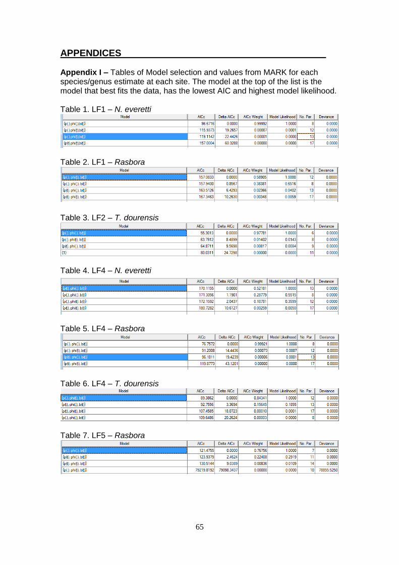
65

APPENDICES Appendix I – Tables of Model selection and values from MARK for each species/genus estimate at each site. The model at the top of the list is the model that best fits the data, has the lowest AIC and highest model likelihood. Table 1. LF1 – N. everetti

Table 2. LF1 – Rasbora

Table 3. LF2 – T. dourensis

Table 4. LF4 – N. everetti

Table 5. LF4 – Rasbora

Table 6. LF4 – T. dourensis

Table 7. LF5 – Rasbora

66

Table 8. Merbau – N. everetti

Table 9. Merbau – Rasbora Table 10. VJR – N.everetti

Table 11. VJR – Rasbora

Table 12. VJR – T. dourensis

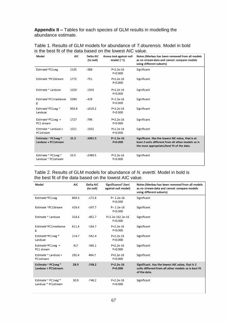
67

Appendix II – Tables for each species of GLM results in modelling the abundance estimate. Table 1. Results of GLM models for abundance of T.dourensis. Model in bold is the best fit of the data based on the lowest AIC value.

Table 2. Results of GLM models for abundance of N. evertti. Model in bold is the best fit of the data based on the lowest AIC value.

68

Table 3. Results of GLM models for abundance of Rasbora. Model in bold is the best fit of the data based on the lowest AIC value.

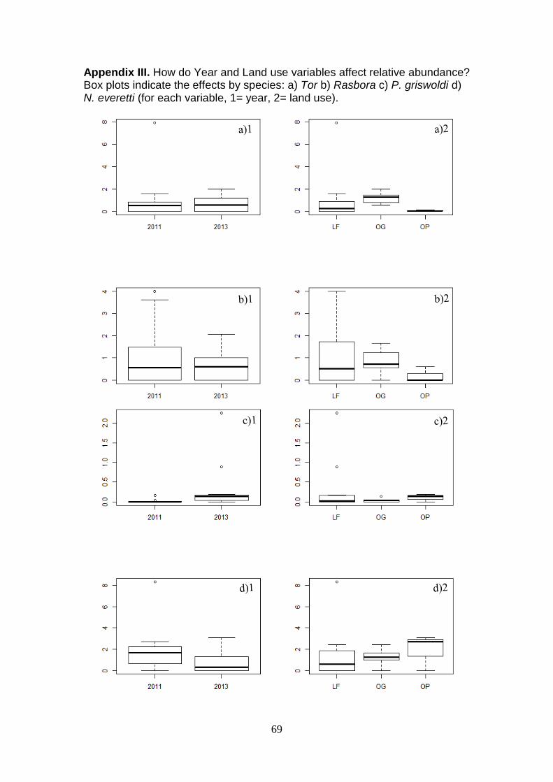
69

Appendix III. How do Year and Land use variables affect relative abundance? Box plots indicate the effects by species: a) Tor b) Rasbora c) P. griswoldi d) N. everetti (for each variable, 1= year, 2= land use).