PROJECT STATIC DEFORMATIONS AND VIBRATION ANALYSIS OF COMPOSITE AND SANDWICH PLATES USING A LAYER WISE THEORY AND RBF-PS DISCRETIZATIONS WITH OPTIMAL SHAPE PARAMETER COMPILED BY KHURAM HINA JANJUA [1] , FOZIA MUNAWAR [2] , MUNIZA AKBAR [3] DEPARTMENT OF MATHEMATICS FRONTIER WOMEN UNIVERSITY COMPOSITE STRUCTURES

Welcome message from author
This document is posted to help you gain knowledge. Please leave a comment to let me know what you think about it! Share it to your friends and learn new things together.
Transcript
PROJECT
STATIC DEFORMATIONS AND VIBRATION ANALYSIS OF COMPOSITE ANDSANDWICH PLATES USING A LAYER WISE THEORY AND RBF-PS
DISCRETIZATIONS WITH OPTIMAL SHAPE PARAMETER
COMPILED BYKHURAM HINA JANJUA[1], FOZIA MUNAWAR[2], MUNIZA AKBAR[3]
DEPARTMENT OF MATHEMATICSFRONTIER WOMEN UNIVERSITY
COMPOSITE STRUCTURES
COMPOSITE STRUCTURES
PESHAWAR
ABSTRACT
This article presents static deformation and free vibration ofshear-deformable or flexible isotropic and laminated compositeplates using layer-wise theory (for laminated/sandwich plates).In order to produce highly accurate results, the approximation ismade by a pseudo spectral method known as radial basis functionsfor the analysis of composite laminates. To optimize the shapeparameter of the basis function (used in RBF-PS method), a cross-validation technique is used. Numerical results for symmetriclaminated composites and sandwich plates are also presented toshow the performance of the method.
COMPOSITE STRUCTURES
ARTICLE OUTLINE
1. INTRODUCTION
2. RBF-PS METHODS
3. FINDING AN ‘OPTIMAL’ SHAPE PARAMETER
4. A LAYERWISE THEORY
5. FREE VIBRATION ANALYSIS
6. INTERPOLATION OF DIFFERENTIAL EQUATIONS OF MOTION AND BOUNDARY
CONDITIONS BY RADIAL BASIS FUNCTIONS
7. CONCLUSIONS

COMPOSITE STRUCTURES
COMPOSITE STRUCTURES
1.INTRODUCTION
In the past two decades, composites have found increasingapplication in many engineering structures. Recent advances inthe technologies of manufacturing and materials have enhanced thecurrent application of composite materials. The compositestructures have become widely known among manufacturers,designers and researchers involved in structures that are formedby using composite materials. Due to the property of nonhomogeneity and anisotropy (having a different value whenmeasured in different directions) of the materials, analysis ofthese composite structures imposes new challenges on engineers.The shear deformation theories are used rapidly in static anddynamic composite and sandwich laminates due to the high ratio ofstiffness in elastic materials. To analyze the compositelaminates, plate and shell structures made of laminated compositematerials have often been modeled by using classical laminatetheory (CLT) and the first order shear deformation theory. Theclassical theory of plates assumes that the normal to the mid-plane before deformation remains straight and normal to the planeafter deformation, under-predicts deflections and over- predictsnatural frequencies and buckling loads. These discrepancies arisedue to the neglect of transverse shear strains. The range ofapplicability of the CLT solution has been well established forlaminated plates by Reddy in 1984. To overcome the deficienciesin CLT, higher order laminate theories have been proposed (mostrecent in 1999).The use of higher order theories is beneficial regarding thewrapping of the normal to the middle surface. These theories havethe advantage of neglecting shear correction factors and producemore promising results for accurate transverse shear stress.These are single-layer theories in which the transverse shearstresses are taken into account. They provide improved globalresponse estimates for deflections, vibration frequencies, andbuckling loads of moderately thick composites when compared withthe CLT.All these theories (i.e. classical laminate plate theory, first-order shear deformation theory and higher-order deformationtheories) also consider laminate-wise or layer-wise rotation. Due
COMPOSITE STRUCTURES
to the difference between the materials properties in laminatesparticularly in sandwich plates, the layer-wise theories areapplied which provide the independent degree of freedom for eachlayer. To analyze the laminated composite plates or sandwichplates, the layer-wise theory proposed by Reddy is considered themost popular while other layer-wise or zigzag theories have beenpresented by Mau, Chou and Corleone, Di Sciuva, Murakami, andRen. The latest theories based on the analysis of multilayeredplates and shells have been presented by Carrera. In this article we adopt a Mindlin type first-order transverseshear deformation theory (SDT) which is a layer-wise theory basedon an expansion of SDT in each layer. A transverse SDT accountsfor the warping of the deformed normal which is required foraccurate prediction of the elastic behavior of multilayeredanisotropic plates and shells. The displacement field iscontinuous at layer’s interface and produces highly accuratetransverse shear stress in each layer middle surface.The discretization techniques for space are normally based onfinite differences and finite elements but in this article weapproach to a new technique where approximation is made by radialbasis functions, viewed as pseudo-spectral method in which layer-wise theory is implemented in order to get the most accurateresults. Further to optimize the shape parameter for the basisfunctions (used in RBF-PS method), we use a cross-validationtechnique named Rippa’s strategy.
The radial basis function method was initially implemented on ageographical scattered data in order to interpolate it. This wasdone by Hardy. Later, Kansa used this method for finding thesolutions of partial differential equations and so far thismethod has been used for solving numerous engineering problems.Liu et al and Ferreira proposed that the radial basis functionsfor two-dimensional solids can also be used for the composite andlaminated plates and beams using the first-order and the third-order shear deformation theory. Recently Ferreira et al has alsoproposed the use of layer-wise theory and radial basis functionsfor the static deformations of composite plates in bending.A summary of this article follows the combination of the layer-wise theory for plates, a RBF-PS Method and an optimization
COMPOSITE STRUCTURES
technique of the shape parameter. The next section discusses thedevelopment of constitutive matrices for composite laminates.Then several numerical examples are presented to demonstrate therange of applicability and accuracy of the proposed theory, andfinally conclusions will be drawn.
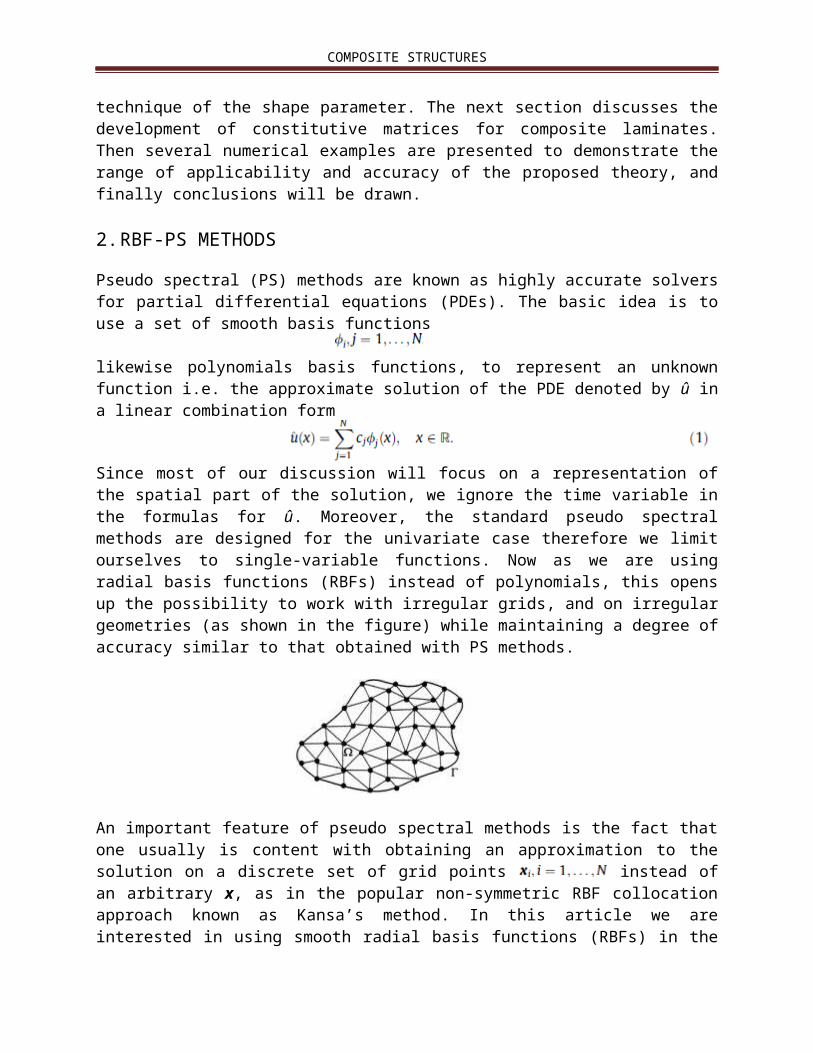
2.RBF-PS METHODS
Pseudo spectral (PS) methods are known as highly accurate solversfor partial differential equations (PDEs). The basic idea is touse a set of smooth basis functions
likewise polynomials basis functions, to represent an unknownfunction i.e. the approximate solution of the PDE denoted by û ina linear combination form
Since most of our discussion will focus on a representation ofthe spatial part of the solution, we ignore the time variable inthe formulas for û. Moreover, the standard pseudo spectralmethods are designed for the univariate case therefore we limitourselves to single-variable functions. Now as we are usingradial basis functions (RBFs) instead of polynomials, this opensup the possibility to work with irregular grids, and on irregulargeometries (as shown in the figure) while maintaining a degree ofaccuracy similar to that obtained with PS methods.
An important feature of pseudo spectral methods is the fact thatone usually is content with obtaining an approximation to thesolution on a discrete set of grid points instead ofan arbitrary x, as in the popular non-symmetric RBF collocationapproach known as Kansa’s method. In this article we areinterested in using smooth radial basis functions (RBFs) in the
COMPOSITE STRUCTURES
spectral expansion (1), with imposing the boundaryconditions (Dirichlet BCs) for the PDE, showing that the PDE andits boundary conditions are satisfied at a set of collocationpoints. This will lead to a system of linear equations which wesolve for the expansion coefficients cj in (1). Once thesecoefficients are found, we can then evaluate the approximatesolution û at any point x by way of (1). So by Kansa’scollocation approach finally we will have an approximate solutionin terms of a (continuous) function. Now we consider the linear elliptic PDE problem
(2)with Dirichlet boundary condition
(3)We are using (infinitely smooth) radial basis functions (RBFs) inthe spectral expansion (1), i.e.
(4)where the points are the centers of the basic functions
and φ is some positive definite univariate basicfunction (or one of the usual radial basis functions). Popularchoices for positive definite functions include inversemultiquadric
(5)the Gaussian
(6)or compactly supported Wendland functions such as
(7)with some additional notational effort all that follows [i.e.(5), (6) and (7)] can also be formulated for conditionallypositive definite functions such as the popular multiquadric
(8)Above, the univariate variable r is a radial variable, i.e., r =x and the positive parameter ε is equivalent to the well-knownshape parameter used to scale the basic functions. We have chosenthe representations above since then ε → 0 always results in“flat” basic functions and it is exactly for this limiting case
COMPOSITE STRUCTURES
that the connection to polynomials mentioned at the beginning ofthis section arises. Since the compactly supported Wendlandfunctions possess only a limited amount of smoothness they willnot be able to provide the full spectral accuracy thatpolynomials and the other infinitely smooth basis functions areable to. However, the experiments below show that they stillprovide very high accuracy, and moreover behave in a more stableway than the other basis functions which proved to be beneficialfor our Eigen value analysis.
Differentiation Matrices:
Now here we will focus on the discussion of differentiationmatrices. Consider expansion (4) where φ is an arbitrary linearlyindependent set of smooth functions that will serve as the basisfor our approximation space. If we evaluate (4) at the gridpoints , then we get
or in matrix-vector notation(9)
where is the coefficient vector, the evaluation matrix A has entries , and
is a vector of values of the approximate solution atthe collocation points.One of several ways to implement the spectral method is the wayof differentiation matrices, i.e. one finds a matrix L such thatat the grid points , we have
(10)
where is the vector of values of û at the gridpoints , and is the vector of values of the‘‘derivatives” of u at the same points .Now in order to get the discrete form of the considered PDE, wewill use the differentiation matrix L and get the discretizedform of the given PDE
(11)
COMPOSITE STRUCTURES
where u is same vector of values of û at the grid points, and f is the vector of values of the right-hand side of theconsidered PDE, evaluated at the collocation points.To compute the derivative of û we can use the expansion (4) bydifferentiating the smooth basis functions. The differentialoperator will be applied on both sides of the original PDEand following the linearity property of derivatives, we get
(12)If we evaluate (12) at the grid points then we get asystem of linear algebraic equations having the matrix-vectornotation
(13)where is the coefficient vector, is avector of values of the approximate solution at the collocationpoints and the matrix has the entries in the case of radialbasis functions as In order to obtain the differentiation matrix L we need to ensureinvertibility of the evaluation matrix A. This depends both onthe basis functions chosen as well as the location of the gridpoints . For univariate polynomials it is well-known thatthe evaluation matrix is invertible for any set of distinct gridpoints. For positive definite radial basis functions, theinvertibility of the matrix A for any set of distinct grid pointsis guaranteed (by Buchner’s theorem). Thus we can use (9) tosolve for the coefficient vector , and then (13) yields
(14)so that the differentiation matrix L corresponding to (10) isgiven by .The matrix L inverts the standard RBF interpolation matrix A,which is clearly nonsingular for all the distributions of centersξj and collocation points . Therefore, we will notconsider the problems of possible non-invertibility of thecollocation matrix that interact with Kansa method.
PDE with Dirichlet Boundary Conditions via RBF-PS Method:
Now we discuss the linear elliptic PDE problem
COMPOSITE STRUCTURES
with Dirichlet boundary condition
We start with the differentiation matrix L based on all gridpoints , and replace the diagonal entries correspondingto the boundary points with ones and the remaining entries ofthose rows with zeros. This corresponds to enforcing the boundarycondition u = g explicitly and we replace the corresponding on the right-hand side by . This will work obviously becausethe resulting product of (boundary) row k of L with the vector unow corresponds to . The resulting matrix LBC which alsoenforces the boundary condition is very closely related to theKansa matrix (which starts with the expansion
(15)The coefficient vector c is determined by inserting (15) into thePDE and boundary conditions and forcing these equations to besatisfied at the grid points . The collocation solutionis therefore obtained by solving a linear system of theseequations) i.e., after a possible permutation of rows we obtain
(16)where , = =The block matrix on the right-hand side is exactly Kansa’smatrix. In order to get the collocation solution of theconsidered linear elliptic problem (2) with the Dirichlet BCs(3), we compute
(17)
implies that , (18)
implies that(19)
The vectors f and g collect the values of f and g at therespective grid points. The last result [i.e. (19)] shows thesolution of discretized PDE (with the differential operatorand Dirichlet BCs) which is exactly to the result when theapproximate solution for the non-symmetric collocation method
COMPOSITE STRUCTURES
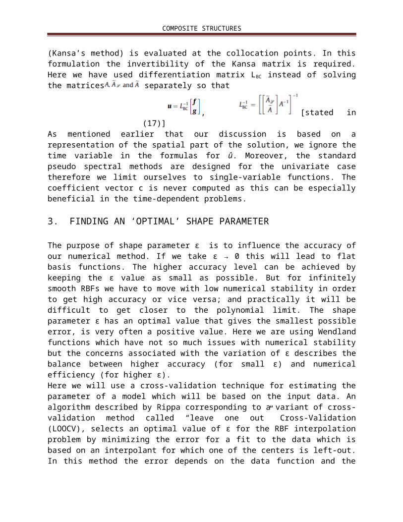
(Kansa’s method) is evaluated at the collocation points. In thisformulation the invertibility of the Kansa matrix is required.Here we have used differentiation matrix LBC instead of solvingthe matrices separately so that
, [stated in(17)]
As mentioned earlier that our discussion is based on arepresentation of the spatial part of the solution, we ignore thetime variable in the formulas for û. Moreover, the standardpseudo spectral methods are designed for the univariate casetherefore we limit ourselves to single-variable functions. Thecoefficient vector c is never computed as this can be especiallybeneficial in the time-dependent problems.
3. FINDING AN ‘OPTIMAL’ SHAPE PARAMETER
The purpose of shape parameter ԑ is to influence the accuracy ofour numerical method. If we take ԑ → 0 this will lead to flatbasis functions. The higher accuracy level can be achieved bykeeping the ԑ value as small as possible. But for infinitelysmooth RBFs we have to move with low numerical stability in orderto get high accuracy or vice versa; and practically it will bedifficult to get closer to the polynomial limit. The shapeparameter ԑ has an optimal value that gives the smallest possibleerror, is very often a positive value. Here we are using Wendlandfunctions which have not so much issues with numerical stabilitybut the concerns associated with the variation of ԑ describes thebalance between higher accuracy (for small ԑ) and numericalefficiency (for higher ԑ). Here we will use a cross-validation technique for estimating theparameter of a model which will be based on the input data. Analgorithm described by Rippa corresponding to a variant of cross-validation method called “leave one out” Cross-Validation(LOOCV), selects an optimal value of ԑ for the RBF interpolationproblem by minimizing the error for a fit to the data which isbased on an interpolant for which one of the centers is left-out.In this method the error depends on the data function and the
COMPOSITE STRUCTURES
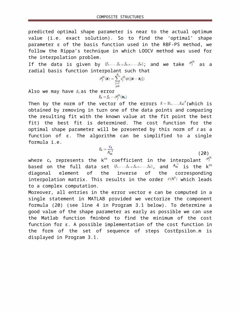
predicted optimal shape parameter is near to the actual optimumvalue (i.e. exact solution). So to find the ‘optimal’ shapeparameter ԑ of the basis function used in the RBF-PS method, wefollow the Rippa’s technique in which LOOCV method was used forthe interpolation problem.If the data is given by ; and we take as aradial basis function interpolant such that
Also we may have Ek as the error
Then by the norm of the vector of the errors (which isobtained by removing in turn one of the data points and comparingthe resulting fit with the known value at the fit point the bestfit) the best fit is determined. The cost function for theoptimal shape parameter will be presented by this norm of E as afunction of ԑ. The algorithm can be simplified to a singleformula i.e.
(20)where ck represents the kth coefficient in the interpolant based on the full data set , and is the kth
diagonal element of the inverse of the correspondinginterpolation matrix. This results in the order which leadsto a complex computation.Moreover, all entries in the error vector e can be computed in asingle statement in MATLAB provided we vectorize the componentformula (20) (see line 4 in Program 3.1 below). To determine agood value of the shape parameter as early as possible we can usethe Matlab function fminbnd to find the minimum of the costfunction for ԑ. A possible implementation of the cost function inthe form of the set of sequence of steps CostEpsilon.m isdisplayed in Program 3.1.
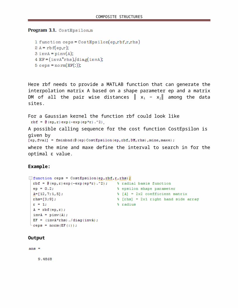
COMPOSITE STRUCTURES
Here rbf needs to provide a MATLAB function that can generate theinterpolation matrix A based on a shape parameter ep and a matrixDM of all the pair wise distances xi − xj among the datasites.
For a Gaussian kernel the function rbf could look like .A possible calling sequence for the cost function CostEpsilon is given by
where the mine and maxe define the interval to search in for theoptimal ԑ value.
Example:
Output
COMPOSITE STRUCTURES
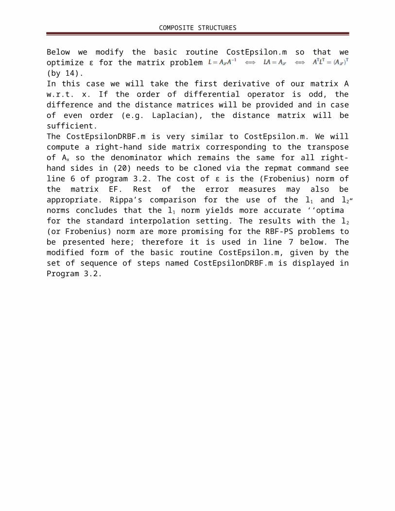
Below we modify the basic routine CostEpsilon.m so that weoptimize ԑ for the matrix problem (by 14). In this case we will take the first derivative of our matrix Aw.r.t. x. If the order of differential operator is odd, thedifference and the distance matrices will be provided and in caseof even order (e.g. Laplacian), the distance matrix will besufficient. The CostEpsilonDRBF.m is very similar to CostEpsilon.m. We willcompute a right-hand side matrix corresponding to the transposeof Ax so the denominator which remains the same for all right-hand sides in (20) needs to be cloned via the repmat command seeline 6 of program 3.2. The cost of ԑ is the (Frobenius) norm ofthe matrix EF. Rest of the error measures may also beappropriate. Rippa’s comparison for the use of the l1 and l2
norms concludes that the l1 norm yields more accurate ‘‘optima”for the standard interpolation setting. The results with the l2
(or Frobenius) norm are more promising for the RBF-PS problems tobe presented here; therefore it is used in line 7 below. Themodified form of the basic routine CostEpsilon.m, given by theset of sequence of steps named CostEpsilonDRBF.m is displayed inProgram 3.2.
COMPOSITE STRUCTURES
Example:
Output:
A program (3.3) that computes the differentiation matrix (withoptimal ԑ) and calls CostEpsilonDRBF as given below.
COMPOSITE STRUCTURES
Example:
COMPOSITE STRUCTURES
Output:
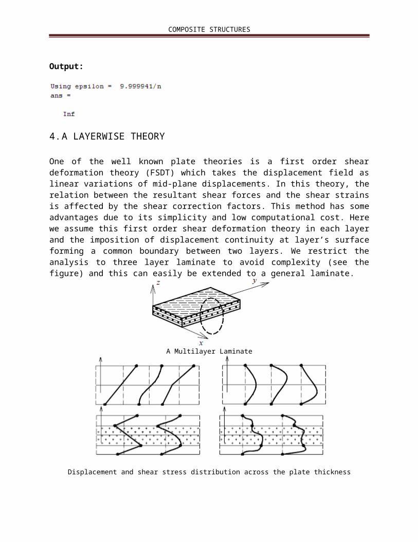
4.A LAYERWISE THEORY
One of the well known plate theories is a first order sheardeformation theory (FSDT) which takes the displacement field aslinear variations of mid-plane displacements. In this theory, therelation between the resultant shear forces and the shear strainsis affected by the shear correction factors. This method has someadvantages due to its simplicity and low computational cost. Herewe assume this first order shear deformation theory in each layerand the imposition of displacement continuity at layer’s surfaceforming a common boundary between two layers. We restrict theanalysis to three layer laminate to avoid complexity (see thefigure) and this can easily be extended to a general laminate.
A Multilayer Laminate
Displacement and shear stress distribution across the plate thickness
COMPOSITE STRUCTURES
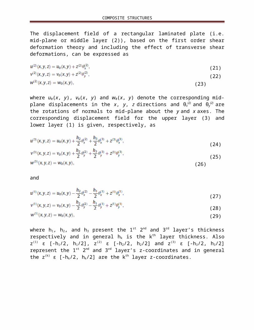
The displacement field of a rectangular laminated plate (i.e.mid-plane or middle layer (2)), based on the first order sheardeformation theory and including the effect of transverse sheardeformations, can be expressed as
(21)(22)
(23)
where u0(x, y), v0(x, y) and w0(x, y) denote the corresponding mid-plane displacements in the x, y, z directions and θx
(2) and θy(2) are
the rotations of normals to mid-plane about the y and x axes. Thecorresponding displacement field for the upper layer (3) andlower layer (1) is given, respectively, as
(24)
(25)(26)
and
(27)
(28)(29)
where h1, h2, and h3 present the 1st 2nd and 3rd layer’s thicknessrespectively and in general hk is the kth layer thickness. Alsoz(1) ϵ [-h1/2, h1/2], z(2) ϵ [-h2/2, h2/2] and z(3) ϵ [-h3/2, h3/2]represent the 1st 2nd and 3rd layer’s z-coordinates and in generalthe z(k) ϵ [-hk/2, hk/2] are the kth layer z-coordinates.
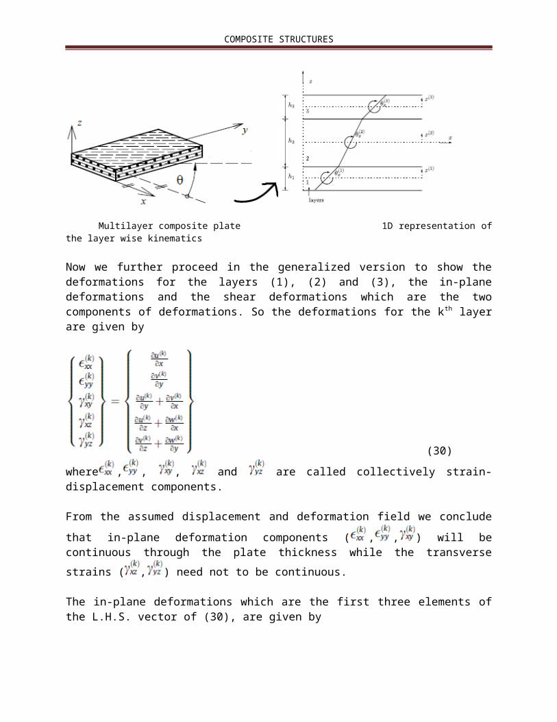
COMPOSITE STRUCTURES
Multilayer composite plate 1D representation ofthe layer wise kinematics
Now we further proceed in the generalized version to show thedeformations for the layers (1), (2) and (3), the in-planedeformations and the shear deformations which are the twocomponents of deformations. So the deformations for the kth layerare given by
(30)where , , , and are called collectively strain-displacement components.
From the assumed displacement and deformation field we concludethat in-plane deformation components ( , , ) will becontinuous through the plate thickness while the transversestrains ( , ) need not to be continuous.
The in-plane deformations which are the first three elements ofthe L.H.S. vector of (30), are given by
COMPOSITE STRUCTURES
(31)
The shear deformations which are the last two elements of theL.H.S. vector of (30), are given by
(32)
Now from the R.H.S. of (31) we have membrane components, bendingcomponents and membrane-bending coupling components respectivelyin the form of vectors as mentioned below.
The membrane components are given by
(33)
The bending components are given by
(34)
And the membrane-bending coupling components for the layers 2(middle layer), 3 (upper layer) and 1 (lower layer) by using (24)and (25) for the upper layer and (27) and (28) for the lowerlayer are given as
COMPOSITE STRUCTURES
(For the middle layer)(35)
(For the upper layer)(36)
(For the lower layer)(37)
Constitutive Equations of Lamina:
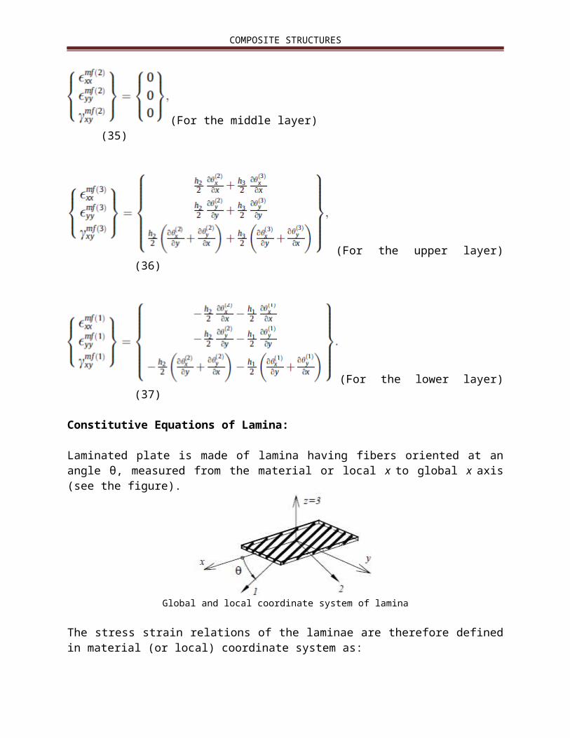
Laminated plate is made of lamina having fibers oriented at anangle θ, measured from the material or local x to global x axis(see the figure).
Global and local coordinate system of lamina
The stress strain relations of the laminae are therefore definedin material (or local) coordinate system as:
COMPOSITE STRUCTURES
(38)
where
are the stress components of kthlamina in material (or local) coordinates.
are the strain components of kthlamina in material (or local) coordinates.
The subscript 1 is the fiber in-plane direction.The subscript 2 is the normal to the fiber in-plane direction.The subscript 3 is the direction normal to the plate.
The Qij(k) matrix of material elastic coefficients (or reduced
stiffness components) for kth laminate is given as:
where
are Young's moduli in 1 and 2 directions,respectively.
COMPOSITE STRUCTURES
Vij(k) are Poisson's ratio defined as ratio of transverse
strain in j-direction to axial strain in i-direction(i,j = 1,2,3).
and are the shear moduli in the 1-2, 2-3 and 3-1planes, respectively.These are collectively called the material properties of lamina k(the kth layer of the laminate k).
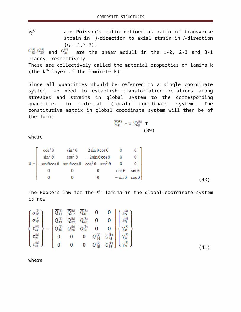
Since all quantities should be referred to a single coordinatesystem, we need to establish transformation relations amongstresses and strains in global system to the correspondingquantities in material (local) coordinate system. Theconstitutive matrix in global coordinate system will then be ofthe form:
(39)
where
(40)
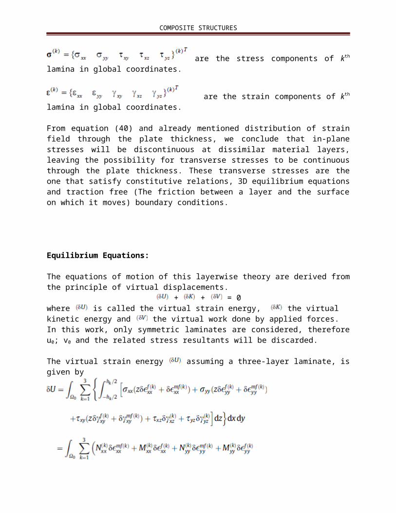
The Hooke's law for the kth lamina in the global coordinate systemis now
(41)
where
COMPOSITE STRUCTURES
are the stress components of kthlamina in global coordinates.
are the strain components of kthlamina in global coordinates.
From equation (40) and already mentioned distribution of strainfield through the plate thickness, we conclude that in-planestresses will be discontinuous at dissimilar material layers,leaving the possibility for transverse stresses to be continuousthrough the plate thickness. These transverse stresses are theone that satisfy constitutive relations, 3D equilibrium equationsand traction free (The friction between a layer and the surfaceon which it moves) boundary conditions.
Equilibrium Equations:
The equations of motion of this layerwise theory are derived fromthe principle of virtual displacements.
+ + = 0where is called the virtual strain energy, the virtual kinetic energy and the virtual work done by applied forces.In this work, only symmetric laminates are considered, thereforeu0; v0 and the related stress resultants will be discarded.
The virtual strain energy assuming a three-layer laminate, isgiven by
COMPOSITE STRUCTURES
(42)
We assume that distributed load acts in the middle surface Ω0 andthe stress resultants are given as:
Similarly we assume for M xx, M yy, M xy. And collectively we have
and (42[a])
(42[b])
where α and β take the symbols x and y.
The virtual kinetic energy assuming a three-layer laminate,is given by
(43)
where ρ(k) is the mass density of the material.
The virtual work done by applied forces assuming a three-layer laminate, are given by
(44)where q is the external distributed load.
COMPOSITE STRUCTURES
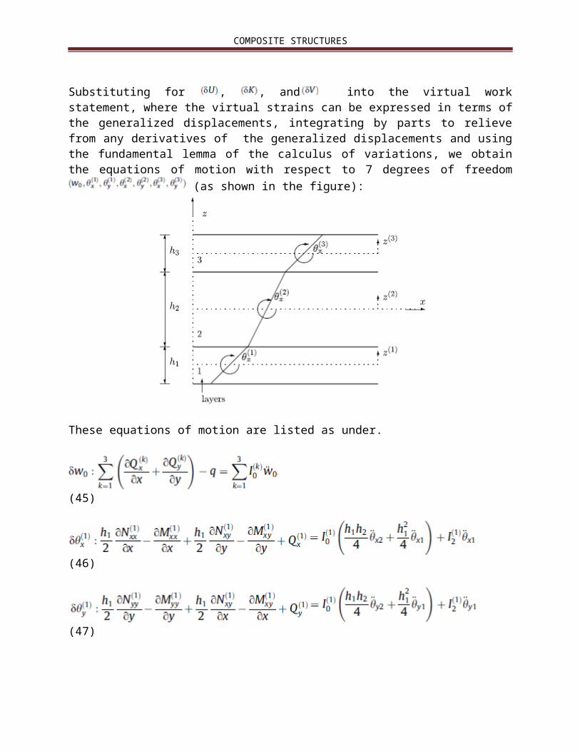
Substituting for , , and into the virtual workstatement, where the virtual strains can be expressed in terms ofthe generalized displacements, integrating by parts to relievefrom any derivatives of the generalized displacements and usingthe fundamental lemma of the calculus of variations, we obtainthe equations of motion with respect to 7 degrees of freedom
(as shown in the figure):
These equations of motion are listed as under.
(45)
(46)
(47)
COMPOSITE STRUCTURES
(48)
(49)
(50)
(51)
where
(52)
where ρ(k) is the mass density of the material and hk thethickness of the kth layer.
The equations of motion can be written in terms of thedisplacements by substituting for strains and stress resultantsinto the equations (45) to (51).
For example, the first equation can be replaced by
COMPOSITE STRUCTURES
(53)
Here the layer-wise theory ends.
5.FREE VIBRATION ANALYSIS
For the analysis of free vibration problems, harmonic solution interms of displacements are assumed in the form
(54)
(55)
(56)
where ω in the exponent denotes the frequency of naturalvibration. Eliminating the external force q and substituting theharmonic expansion into equations of motion (45) to (51), weobtain (53) in terms of the amplitudes , where k = 1,2,3.
(57)
Similarly we proceed for rest of the equations of motion.
6. INTERPOLATION OF DIFFERENTIAL EQUATIONS OF MOTION ANDBOUNDARY CONDITIONS BY RADIAL BASIS FUNCTIONS
An important feature of pseudo spectral methods is the fact thatone usually is content with obtaining an approximation to thesolution on a discrete set of grid points instead of

COMPOSITE STRUCTURES
an arbitrary x, as in the popular non-symmetric RBF collocationapproach used in this article known as Kansa’s method. We areusing (infinitely smooth) radial basis functions (RBFs) in thespectral expansion i.e.
where the points are the centers of the basic functions and φ is some positive definite univariate basic
function (or one of the usual radial basis functions). Theinterpolation of equations of motion is now done by radial basisfunctions, for each node i. For example, (57) is expressed as
(58)
Rest of the six equations are interpolated in the same way. Thevector of unknowns is now composed of the interpolationparameters ɑj, for respectively. The RBFinterpolation is a simple process for each boundary node. As anexample, a simply-supported condition at x = β edge with outwardnormal direction α imposes seven boundary conditions as follows:
1.
2.
3.
or equivalently we have
4.
COMPOSITE STRUCTURES
5.
6.
The RBF interpolation of boundary equations leads to a change inthe global equations system. For each node i where the equationsare valid, the following equations are imposed.For example, the boundary condition (1) is interpolated as
7.
where N represents the total number of grid points.Similarly rest of the boundary conditions (2 - 7) can beinterpolated.
7. CONCLUSION
In this paper, for the first time the free vibration analysis ofcomposite laminated plates by the use of RBFs in a pseudospectralmethod and using a layerwise theory with independent rotations ineach layer is performed. The MatLab implementation including three programs has beendeveloped in order to analyze the optimal shape parameter. In thelayerwise theory the equations of motion were derived and solvedby the RBF collocation method and next the interpolation of theboundary conditions was formulated in a simplified manner. Themethod produces highly accurate results for isotropic, laminatedcomposites and sandwich plates.
Related Documents