Composite Likelihood Estimation of AR-Probit Model: Application to Credit Ratings * Kerem Tuzcuoglu † April 21, 2017 Abstract In this paper, persistent discrete data are modeled by Autoregressive Probit model and esti- mated by Composite Likelihood (CL) estimation. Autocorrelation in the latent variable results in an intractable likelihood function containing high dimensional integrals. CL approach offers a fast and reliable estimation compared to computationally demanding simulation methods. I provide consistency and asymptotic normality results of the CL estimator and use it to study the credit ratings. The ratings are modeled as imperfect measures of the latent and autocorrelated creditworthiness of firms explained by the balance sheet ratios and business cycle variables. The empirical results show evidence for rating assignment according to Through-the-cycle methodol- ogy, that is, the ratings do not respond to the short-term fluctuations in the financial situation of the firms. Moreover, I show that the ratings become more volatile over time, in particular after the crisis, as a reaction to the regulations and critics on credit rating agencies. Keywords: Composite likelihood, autoregressive probit, autoregressive panel probit, stability of credit ratings, through-the-cycle methodology JEL Classification: C23, C25, C58, G24, G31 * I would like to thank Serena Ng, Jushan Bai, Bernard Salani´ e, Sokbae Lee, J´ on Steinsson, Aysun Alp, as well as seminar participants at Columbia University, for their comments and suggestions. All errors are, of course, my own. † Ph.D. Candidate, Economics Department, Columbia University [email protected].

Welcome message from author
This document is posted to help you gain knowledge. Please leave a comment to let me know what you think about it! Share it to your friends and learn new things together.
Transcript

Composite Likelihood Estimation of AR-Probit Model:
Application to Credit Ratings∗
Kerem Tuzcuoglu †
April 21, 2017
Abstract
In this paper, persistent discrete data are modeled by Autoregressive Probit model and esti-
mated by Composite Likelihood (CL) estimation. Autocorrelation in the latent variable results
in an intractable likelihood function containing high dimensional integrals. CL approach offers
a fast and reliable estimation compared to computationally demanding simulation methods. I
provide consistency and asymptotic normality results of the CL estimator and use it to study the
credit ratings. The ratings are modeled as imperfect measures of the latent and autocorrelated
creditworthiness of firms explained by the balance sheet ratios and business cycle variables. The
empirical results show evidence for rating assignment according to Through-the-cycle methodol-
ogy, that is, the ratings do not respond to the short-term fluctuations in the financial situation
of the firms. Moreover, I show that the ratings become more volatile over time, in particular
after the crisis, as a reaction to the regulations and critics on credit rating agencies.
Keywords: Composite likelihood, autoregressive probit, autoregressive panel probit, stability of
credit ratings, through-the-cycle methodology
JEL Classification: C23, C25, C58, G24, G31
∗I would like to thank Serena Ng, Jushan Bai, Bernard Salanie, Sokbae Lee, Jon Steinsson, Aysun Alp, as well asseminar participants at Columbia University, for their comments and suggestions. All errors are, of course, my own.†Ph.D. Candidate, Economics Department, Columbia University [email protected].

1 Introduction
Persistent discrete variables are extensively used in both economics and finance literature. Credit
ratings, changes in the Federal Funds Target Rate, NBER recession dates, unemployment status,
and school grades are just a few important examples among many. These variables have a fair
amount of persistence in them: credit ratings of companies change rarely; the policy rate is usually
adjusted gradually by central banks; a recession (expansion) in a quarter tends to be followed by a
recession (expansion) in the next quarter. To understand the nature of these variables, one needs
to take care of discreteness and persistence at the same time.
But, modeling and estimating persistent discrete data can be challenging. Incorporating time
series concepts (to capture the persistence) into the nonlinear nature of discrete data might need
complex models that are hard to estimate. To deal with such complications, I borrow a method
– composite likelihood estimation – from statistics literature and bring it to economics where the
method is not widely known. Composite likelihood (CL) estimation is a likelihood-based method
that uses the partial specification of full-likelihood. CL becomes very useful especially in cases
where writing or computing the full-likelihood is infeasible, yet marginal or conditional likelihoods
are easier to formulate. In particular, CL can offer a fast and robust estimation for models with
complex likelihood function that can be written only in terms of a large dimensional integral, which
renders implementation of the full-likelihood maximization approach impractical or computation-
ally demanding.
An interesting model with such challenging likelihood is an autoregressive probit (AR-Probit)
model, where discrete (binary or categorical) data are modeled as a nonlinear function of an un-
derlying continuous autoregressive latent process. Mathematically, an AR-Probit model can be
represented as
y∗it = ρy∗i,t−1 + β′xit + εit
yit = 1[y∗it ≥ 0]
where i represents firms, t represents time, and 1(·) represents the indicator function. The discrete
yit can be considered as an imperfect measure of the latent process y∗it. Hence, the autoregressive
property of the latent process drives the persistence in the discrete variable. But, the nonlinear
dynamic dependency between yit and y∗it results in an intractable likelihood function with a high
dimensional integral that does not have an explicit solution. Although there are methods (e.g., sim-
ulated maximum likelihood, Bayesian estimation techniques) to compute/approximate likelihoods
containing integrals, they are computationally demanding. More importantly, they might become
2
unstable and even impractical if the dimension of the integral is large – in the empirical part, my
model has 55 dimensional integral. In this paper, I extend the above model into various directions
and use composite likelihood approach to estimate the complex likelihood of the AR-Probit model.
Lindsay [1988] defined composite likelihood as a likelihood-type object formed by multiplying
together individual component likelihoods, each of which corresponds to a marginal or conditional
event. The merit of CL is to reduce the computational complexity so that it is possible to deal with
large datasets and complex dependencies, especially when the use of standard likelihood methods
are not feasible. The formal definition of composite likelihood is as follows.
Definition 1. Let {f(y; θ), y ∈ Y, θ ∈ Θ} be a parametric statistical model with Y ⊆ RT, Θ ⊆ Rd,
T ≥ 1 and d ≥ 1. Consider a set of events {Ai : Ai ⊆ F , i ∈ I}, where I ⊆ N and F is some sigma
algebra on Y. A composite likelihood is defined as
LC(θ; y) =∏i∈I
f(y ∈ Ai; θ)wi ,
where f(y ∈ Ai; θ) = f({yj ∈ Y : yj ∈ Ai}; θ), with y = (y1, . . . , yT ), while {wi, i ∈ I} is a set of
suitable weights. The associated log-likelihood is LC(θ; y) = log LC(θ; y).
The definition of composite likelihood is very general, even encompassing the full-likelihood as a
special case. Hence, the definition does not tell how to formulate composite likelihood in special
cases; it just states that composite likelihood is a weighted collection of likelihoods. In practice, CL
is chosen as a subset of the full-likelihood. For a T -dimensional data vector y, the most common
choices are marginal composite likelihood LC(θ; y) =∏Tt f(yt|θ) and pairwise composite likelihood
LC(θ; y) =∏Tt=1
∏s 6=t f(yt, ys|θ) or LC(θ; y) =
∏T−Jt=1
∏Jj=1 f(yt, yt+j |θ). In this sense, CL is con-
sidered to be pseudo-likelihood, quasi-likelihood, and partial-likelihood by several authors (Besag
[1974], Cox [1975]). Compared to the traditional maximum likelihood estimator, the CL method
may be statistically less efficient, but consistency, asymptotic normality, and significantly faster
computation are among the appealing properties of the CL estimator. Moreover, it can be more
robust to model misspecification compared to ML estimation or simulation methods since one needs
only correct sub-models in CL approach.
AR-Probit is clearly not the only model to estimate persistent discrete data – though it is more
akin to standard time series models. One can consider replacing the lag of the unobserved vari-
able y∗t−1 by the lag of the observed outcome yt−1. In the literature, this model is called Dynamic
Probit. This is a state-dependence model whereas AR-Probit is closer to habit-persistence models.
Dynamic Probit models are useful when the discrete variable is an important policy variable since
the past discrete observation yt−1 creates a jump in the continuous latent variable. On the other
3
hand, AR-Probit models are useful when the discrete variable is an imperfect measure of the un-
derlying dynamic state variable.
A good example where AR-Probit can be preferred would be credit ratings where the rating
assigned to a firm is an imperfect measure of firm’s underlying creditworthiness evaluated by a
credit rating agency. A firm does receive AA rating not because it was assigned AA previously, but
because the financial situation of the firm is persistent and yields a similar level of credit conditions
as previously. Another example is NBER recession dates. Many papers (e.g., Dueker [1997], Kauppi
and Saikkonen [2008]) use the past recession dummy variable to predict its future values. Here we
should consider this question: “Is the economy in a recession because it was in a recession in the
previous period, or is it because the underlying state of the economy is persistent and was in a bad
state previously?”. A case can be made that, the second argument explains the recessions better.
From this point of view, the AR-Probit seems a better option to model persistent discrete data in
some cases. Moreover, Beck et al. [2001] argued that AR-Probit yields often superior results than
Dynamic Probit. Regarding estimation, maximum likelihood can easily be applied to Dynamic
Probit model (de Jong and Woutersen [2011]) since the discrete data have Markovian property.
However, in AR-Probit model, the discrete data are not Markovian anymore, and the likelihood
contains integrals to be computed or approximated – which can be computationally challenging.
With composite likelihood, in particular, with modeling only pairwise likelihoods, one bypasses the
need for simulations and still achieve an estimator with desirable asymptotic properties.
This paper contributes to two strands of literature. First, it contributes to the composite likeli-
hood literature by providing the consistency and asymptotic normality results of the CL estimator
in the AR-Probit model. CL is gaining substantial attention in the statistics field but has relatively
little coverage in econometrics and other related fields. To be precise, there have been just a handful
of papers that used composite likelihood in the economics and finance literature. Varin and Vidoni
[2008] showed how pairwise likelihood can be applied, from simple models, like AR(1) model with a
dynamic latent process, to more complex ones, like AR-Tobit model. That paper can be considered
an introduction of composite likelihood approach to econometrics literature. Afterwards, Engle
et al. [2008] and Pakel et al. [2011] both utilized CL estimator in multivariate GARCH models to
avoid inverting large-dimensional covariance matrices. Bhat et al. [2010] compared the performance
of simulated maximum likelihood (SML) to CL in a Panel Probit model with autocorrelated error
structure and found that CL needs much less computational time and provides more stable esti-
mation (see Reusens and Croux [2016] for an application of this model to sovereign credit ratings).
CL is attractive to estimate DSGE models, in particular with stochastic singularities (Qu [2015])
or misspecifications (Canova and Matthes [2016]). CL can also be employed to deal with high di-
mensional copulas (Oh and Patton [2016] and Heinen et al. [2014]). Finally, Bel et al. [2016] use CL
4

in a multivariate logit model and show that CL has much smaller computation time with a small
efficiency loss compared to MLE. In statistics literature, Varin and Vidoni [2006] show the appli-
cability and usefulness of CL estimation in AR-Probit model. Standard asymptotic results for CL
estimation under general theory have already been presented in the literature (see Lindsay [1988],
Molenberghs and Verbeke [2005], Varin et al. [2011]). However, finding the required assumptions
and proving the asymptotic results of CL estimator specifically in AR-Probit models, to the best
of my knowledge, is a theoretical contribution. CL, as a general class of estimators, is known to
be consistent and asymptotically normal, but, in this paper, I provide the required assumptions to
achieve these asymptotic results in the AR-Probit model.
Second, this paper contributes to the corporate bond ratings literature by studying the stability
of the ratings in a model with firm specific variables. It is known that there is a trade-off between
accuracy and stability of credit ratings (Cantor and Mann [2006]). More accurate ratings require
more volatility in rating assignments to capture the changes in the creditworthiness of companies in
a timely fashion. This paper contributes by presenting a new methodology and findings in measuring
stability. In particular, to the best of my knowledge, this is the first paper at the firm-level analysis,
where the rating stability is measured by a single estimated coefficient – the persistence parameter ρ.
Moreover, by using time-varying coefficients (ρt), the rating stability changes is estimated over time.
But, why is the rating stability important? The rating stability has its benefits for investors, issuers,
and credit rating agencies. Moreover, rating stability is desirable to prevent pro-cyclical effects in
the economy – ratings that respond to temporary information might exacerbate the situation and
contribute to the market volatility. For this reason, credit rating agencies promised to assign ratings
according to Through-the-cycle (TTC) methodology1, which means that the ratings do not reflect
short-term fluctuations, but rather indicate the long-term trustworthiness of a firm (see Altman and
Rijken [2006] for more details on TTC). The literature is divided on verifying TTC rating claim
by rating agencies. A branch of literature found evidence for pro-cyclical ratings, thus argues that
rating agencies uses Point-in-time (PIT)methodology instead of TTC (Nickell et al. [2000], Bangia
et al. [2002], Amato and Furfine [2004], Feng et al. [2008], Topp and Perl [2010], Freitag [2015]).
On the other hand, there are others showing that rating agencies can in fact see through the cycle
(Carey and Hrycay [2001], Altman and Rijken [2006], Loffler [2004, 2013], and Kiff et al. [2013]). In
this paper, I provide empirical evidence for TTC rating approach by showing that during the Great
Recession, rating agencies actually tried to hold the ratings stable for the first 2-3 quarters of the
recession before starting downgrading the firms. Only afterward, when rating agencies realized that
the changes in the credit situation of the firms are not short-term, ratings are let to be more volatile.
1Standard and Poor’s [2002, p.41]: “The ideal is to rate through the cycle. There is no point in assigning highratings to a company enjoying peak prosperity if that performance level is expected to be only temporary. Similarly,there is no need to lower ratings to reflect poor performance as long as one can reliably anticipate that better timesare just around the corner.”
5

The rest of the paper proceeds as follows. Section 2 gives an overview of the composite likelihood
approach and the advantages over other estimation techniques. Section 3 introduces the Panel AR-
Probit model, explains how to construct the pairwise composite likelihood, and states the theoretical
asymptotic results. The last large section is dedicated to the empirical application. In that section,
extensions of the baseline model are provided together with the estimation results and robustness
checks. All the mathematical proofs are left to the Technical Appendix.
2 Composite Likelihood Literature
The literature on composite likelihood goes back to late 1980s, but it became popular especially
after the early 2000s. The papers using CL are mostly focused on statistics, computer science, and
biology to handle the estimation of very complex systems. In the economics literature, and more so
in finance, CL is relatively an unknown topic. The first paper that defines composite likelihood is
Lindsay [1988]. CL has its roots in the pseudo-likelihood of Besag [1974] and the partial likelihood
of Cox [1975]. Varin et al. [2011] gives a thorough overview of the topic.
CL has a wide variety of applications, but I will focus on the literature involving models that
have dynamic latent variables; a feature that is present in AR-Probit model. The first example is
Le Cessie and Van Houwelingen [1994], where correlated binary data, even though the underlying
process is not explicitly modeled, is estimated by pairwise likelihoods. Varin and Vidoni [2006],
mentioned above, is the first paper that applied CL to AR-Probit. Varin and Czado [2009] of-
fered pairwise composite likelihood in panel probit model with autoregressive error structure. This
model is also used later in Bhat et al. [2010]. Some theoretical results of CL estimator in a general
class of models with a dynamic latent variable (e.g., stochastic volatility, AR-Poisson) is introduced
in Ng et al. [2011]. Gao and Song [2011] applied EM algorithm to composite likelihood in hidden
Markov models. A dynamic factor structure in a probit model was analyzed in Vasdekis et al. [2012].
Theoretical properties of composite likelihood are closely related to pseudo-likelihoods (see
Molenberghs and Verbeke [2005] for some asymptotic results in general context). Because CL
comprises either marginal or conditional likelihoods which are in fact parts of the full likelihood,
some nice theoretical results directly follow from the properties of the full likelihood. For instance,
CL satisfies the Kullback-Leibler information inequality since log-likelihood of each conditional or
marginal event `i belongs to the full likelihood, thus
IEθ0 [`i(θ)] ≤ IEθ0 [`i(θ0)] for all θ.
6
Kullback-Leibler inequality together with some regular mild assumptions gives consistency of the
CL estimator. However, being a “miss-specified likelihood”, the asymptotic variance of the CL
estimator is not the inverse of the information matrix. Instead, it is in the so-called sandwich form
(it also goes by the name Godambe Information in the statistics literature due to Godambe [1960]).
Regarding hypothesis testing, Wald and score test statistics are standard; however (composite)
likelihood ratio test statistic does not have a χ2 distribution asymptotically. It has a non-standard
asymptotic distribution in the form of a weighted summation of independent χ2 distributions where
the weights are the eigenvalues of the multiplication of the inverse Hessian and the information ma-
trix (see Kent [1982]). Adjustments to CL ratio statistics can also be made so that one obtains
asymptotically a χ2 distribution (see Chandler and Bate [2007] and Pace et al. [2011]). Model
selection can be done according to information criteria such as AIC and BIC with composite like-
lihoods as shown in Varin and Vidoni [2005] and Lindsay et al. [2011]. The information criterion
contains the composite likelihood and a penalty term that depends on the multiplication of the
inverse Hessian and the information matrix.
Composite Likelihood provides computational ease and sometimes even computational possi-
bility of the estimation. Moreover, it is more robust than full likelihood approach since only the
likelihoods that are part of the composite likelihood must be correctly modeled instead of the cor-
rectly specified full likelihood. For instance, a pairwise composite likelihood in AR-Probit model
requires the correct specification of the bivariate probabilities instead of the correct specification
of all dependencies of the data. However, composite likelihood comes with a cost: efficiency loss.
It is hard to establish a general efficiency result for composite likelihoods. Mardia et al. [2007]
show that composite conditional estimators are fully efficient in exponential families that have a
certain closure property under subsetting. For instance, AR(1) model falls into this category; it
is easy to show that the conditional composite likelihood∏Tt=1 f(yt|yt−1) actually is the (condi-
tional) full likelihood in AR(1) model. Lindsay et al. [2011] have a theory on optimally weighting
the composite likelihood to increase the efficiency. However, they stated: “We conclude that the
theory of optimally weighted estimating equations has limited usefulness for the efficiency problem
we address.”. Similarly, Harden [2013] proposed a weighting scheme for composite likelihood but
the simulations showed minimal improvements regarding efficiency. There are several studies for
efficiency on specific examples. For instance, Davis and Yau [2011] analyzed the efficiency loss of
the CL estimator in AR(FI)MA models where both the full-likelihood and the pairwise likelihood
can be computed. They find that in AR models and long-memory processes with a small integration
parameter, the efficiency loss is ignorable. However, CL might have substantial efficiency loss in
MA models and long-memory processes if the order of integration is high. Hjort and Varin [2008]
conjectured that CL can be seen as a penalized likelihood in general Markov chain models and find
that efficiency loss of CL estimator compared to ML is negligible. Joe and Lee [2009] and Varin
7

and Vidoni [2006] find evidence that, in time series context, including only nearly adjacent pairs
in the composite likelihood∏T−Jt=1
∏Jj=1 f(yt, yt+j) might have advantages over all-pairs composite
likelihood∏t6=s f(yt, ys) . The idea follows from the fact that far apart observations bring almost
no information but end up bringing more noise to the estimation.
Identification of the parameters in CL is the most tricky part. So far, the literature has not been
able to provide conditions which guarantee identifiability. Since CL can contain very different com-
ponents of the full likelihood, it is not always clear when identification can or cannot be achieved.
A very simple example helps us understand the issue. Consider an AR(1) model yt = ρyt−1 + σet.
If we choose marginal distribution f(yt) = N (0, σ2/(1 − ρ2)) as CL then we cannot identify the
parameters (ρ, σ) separately. However, using conditional distribution f(yt|yt−1) = N (ρyt−1, σ2) as
CL enables us to identify the parameters. Even in such an easy example, the choice of composite
likelihood matters dramatically in terms of identification. In more complex models, it is not clear,
in general, which sub-likelihoods should be included in the CL so that one can identify all of the
parameters. For now, the identification is checked case by case until a unified theory on identifica-
tion in CL literature is developed.
Composite likelihood might be relatively new in the economics literature, but its underlying
idea of modeling misspecified likelihood has been used for many years under different names like
pseudo-likelihood, partial-likelihood or quasi-likelihood. For instance, asymptotic theory on pseudo
maximum likelihood based on exponential families is analyzed by Gourieroux et al. [1984]. Ferma-
nian and Salanie [2004] suggests estimating parts of the full-likelihood of an autoregressive Tobit
model by nonparametric simulated maximum likelihood. Molenberghs and Verbeke [2005] has a
chapter on pseudo-likelihoods with applications and theoretical results. In the finance literature,
Lando and Skødeberg [2002] used partial-likelihood to estimate some of the parameters from only
a particular part of the likelihood function. In Duan et al. [2012], to avoid intensive numerical
estimations in a forward intensity model, pseudo-likelihood is constructed with overlapping data to
utilize the available data to the fuller extent.
CL is not the only estimation technique to estimate complex models where the full-likelihood
contains large dimensional integral. Simulated maximum likelihood (SML) and Bayesian techniques
have been the most common choices in economics and finance literature to compute these integrals.
In economics, Hajivassiliou and Ruud [1994], Gourieroux and Monfort [1996], Lee [1997], Ferma-
nian and Salanie [2004](non-parametric SML); in finance, Gagliardini and Gourieroux [2005], Feng
et al. [2008], Koopman et al. [2009], and Koopman et al. [2012] (Monte Carlo ML) can be given
as examples among many papers that used SML. One concern about SML in these models is the
computational complexity. In fact, Feng et al. [2008] stated that “Practitioners might, however,
8

find this method complicated and possibly time-consuming.” and “Although the SML estimators
are consistent and efficient for large number of simulations, practitioners may find the procedure
quite difficult and time-consuming.”. Thus they offered an auxiliary estimation where the model is
estimated first without dynamics, then the dynamics of the factor are estimated in a second step.
Bhat et al. [2010] compared the performances of SML (GHK simulator – one of the most frequently
used SML techniques) and CL estimation in a Panel Probit with correlated errors model. The
number of categories for the ordered outcome (yit ∈ {1, . . . , S}) and the time dimension are the
key factors for computation times for SML. Thus they were kept at low levels. In their simulations,
N = 1000, T = 5, and S = 5. The results show that both estimation techniques recovered the
true parameters successfully, and there is almost no difference in efficiency between CL and SML.
This result is interesting since CL is supposed to be less efficient than full-likelihood approach.
However, SML is efficient when the number of draws tends to infinity; otherwise, the simulation
error in approximating the likelihood is not negligible. If one cannot simulate a large number of
times – due to computational power and time restrictions, SML also ends up being inefficient.
Hence, CL and SML provide comparable estimation results, but in terms of computation times, CL
is approximately 40 times faster than SML. In terms of Bayesian techniques, Chauvet and Potter
[2005], Dueker [2005], McNeil and Wendin [2007], and Stefanescu et al. [2009] use Gibbs sampling
in latent dynamic probit models. However, Muller and Czado [2012] showed that in such models,
Gibbs sampler exhibits bad convergence properties, therefore, suggested a more sophisticated group
move multigrid Monte Carlo Gibbs sampler. Yet, this proposed technique was criticized by Varin
and Vidoni [2006] and Bhat et al. [2010] for increasing the computational complexity. Finally, it
is worth to mention that Gagliardini and Gourieroux [2014] proposed an efficient estimator that
does not require any simulation. They used Taylor approximation of the likelihood to estimate,
but their theory needs the following conditions in order the approximation error to become negli-
gible: N → ∞, T → ∞, and T ν/N = O(1) for ν > 1 (or ν > 1.5 for stronger results). However,
in their simulations and applications, they used N = 1000 and T = 20, where T is actually not large.
A final word can be said on the similarity between CL and GMM estimation technique. In
GMM, the researcher should choose the orthogonality conditions to estimate the parameters. How-
ever, selecting the most informative moments is not an easy task (see Andrews [1999] for some
optimality conditions). In this regard, CL is similar to GMM since the researcher should choose
the collection of likelihoods which will be included in the composite likelihood. Moreover, there
is no theory that tells how to choose them optimally. CL is attractive when the model is very
complicated; thus, most of the time, the researcher is already limited by the model complexity or
computational burden. For instance, in an AR-Probit model, one can easily model bivariate and
maybe trivariate probabilities, but computing quadruple probabilities becomes complicated and
reduces the attractiveness of the CL. The composite likelihood (as well as maximum likelihood)
9

estimator can be considered a subset of the method of moment estimators. In particular, one can
always choose the orthogonality conditions for GMM estimation as the score functions derived from
the (composite) likelihood. In this sense, it is hard to pin down the difference between GMM and
CL estimator. However, in panel data applications with strictly exogenous regressors, it is well
known that the orthogonality conditions are of order T 2. In an application like the one in this
paper, where N = 516 and T = 55, the number of moment conditions is extremely high. Not
all moments are informative, but choosing “the best ones” among them is a hard exercise. More-
over, computing the optimal weighting matrix and taking its inverse is practically impossible. This
situation results in a noisy GMM estimation whereas there is not such an issue in CL estimation
since one just adds the log-likelihoods for i = 1, . . . , N and t = 1, . . . , T . Simulation results for a
comparison of CL versus GMM are provided in the following section after introducing the pairwise
composite likelihood estimation. The results clearly favors for the CL estimation in a setting similar
to the empirical application of this paper. As a result, GMM can be considered a set of estimators
that contains MLE and CLE as special cases, however, in some large scale applications, it might be
beneficial to use CL over GMM.
3 Panel AR-Probit Model and Pairwise Composite Likelihood
In this section, I introduce the baseline Panel AR-Probit model and construct a pairwise composite
likelihood. Moreover, I state the objective function to be maximized and the assumptions needed for
consistency and asymptotic normality of the resulting composite likelihood estimator. The proofs
are left to the appendix.
For i = 1, . . . , N and t = 1, . . . , T , let i denotes the ith firm and t denotes the time. I assume that
the innovations are εitiid∼ N (0, 1) over both i and t. The choice of normal distribution is somewhat
important: with the estimation approach that is explained below, the errors should belong to a
family of probability distribution that is closed under convolution. More explanation will be given
at the end of the section. The variance of the innovations is assumed to be 1 in order to identify
other parameters, which is a typical assumption in any probit model. The (K × 1) dimensional
explanatory variables are denoted by xit, and are assumed to be strictly exogenous in the sense
that f(εi|xi) = f(εi), where the notation zi denotes the T -dimensional vector (zi1, . . . , ziT )′. More-
over, the regressors are independent and identically distributed on the cross-section. A univariate,
continuous, latent, autoregressive process y∗it is generated by its lag y∗i,t−1, xit and εit in a linear
relationship. Depending on the level of y∗it, the univariate discrete variable yit is generated. The
((K + 1)× 1) dimensional parameters to be estimated are θ ≡ (ρ, β′)′. Theoretically, |ρ| < 1 is not
required for stationarity since T is fixed. However, when T is at least moderately large, |ρ| < 1 is
needed for empirical stability of the estimator.
10

The continuous variable y∗it is unobserved, however the binary variable yit ∈ {0, 1} is observed.
Hence, an autoregressive panel probit model can be written as, for t = 1, . . . , T ,
y∗it = ρy∗i,t−1 + β′xit + εit, (1)
yit = 1[y∗it ≥ 0]. (2)
The initial condition will be defined below. The generating process of the latent autoregressive y∗it is
Markov, however the same is not true for the discrete value yit. The variable yit depends nonlinearly
on the autoregressive y∗it, thus yit does depend not only on yi,t−1 but also on the whole history of
yit, i.e., on {yi,t−1, . . . , yi1}. In other words, yit exhibits non-Markovian property because yi,t−1
contains only partial information – interval information – concerning y∗it. Therefore, the values
{yi,t−2, . . . , yi1} contain additional imperfect but useful information for yit. Hence, the typical
Markov property in linear time series models is not valid in AR-Probit model. For this reason, one
needs to integrate out y∗it, which results in a T dimensional integral in the likelihood function for
each individual firm i that does not have an explicit analytical solution.
Li(yi|xi; θ) =
∫· · ·∫f(yi|yi
∗; θ)f(yi∗|xi; θ)dyi
∗,
It is not feasible to maximize∑N
i=1 logLi(yi|xi; θ) by maximum likelihood estimation unless T is
fairly small (see Matyas and Sevestre [1996]). For a very small T , one can either compute T -variate
probabilities – it gets exponentially complicated as T enlarges to compute the probability of the
history {yi1, . . . , yiT } – or one can approximate the integrals, say by Gauss–Hermite quadrature.
However, all these solutions are feasible for very small T . One can use simulation-based techniques –
as well as Bayesian – to compute large dimensional integrals, however as mentioned in the previous
sections, these estimation techniques are computationally demanding and might have convergence
issues. Hence, composite likelihood estimation is a good alternative for panel AR-Probit models
with large N and not-so-small T . In particular, a composite likelihood consisting of only pairwise
dependencies will be easy to estimate since the nonlinear dependencies are reduced to a level that
is easy to handle. For instance, a composite likelihood of pairs with at most J-lag distant apart
can be formed by
`i(yi|xi; θ) =
T−J∑t=1
J∑j=1
log f(yit, yi,t+j |xi; θ). (3)
One could write composite likelihood of each pairs f(yit, yis|xi; θ) for s 6= t rather than f(yit, yi,t+j |xi; θ).
However, in a time series framework, the dependency between two observations becomes negligible
as they get more distant. Thus, in practice, all-pairs-likelihood might be even inferior to J-pairs
likelihood in terms of estimated variance (Varin and Vidoni [2006], Joe and Lee [2009]). Before
11

computing the pairwise probabilities in (3), it will be constructive to compute marginal probabilities.
First, since y∗i,t−1 is not observed, I use backward substitution on latent process, that is, the
current laten variable becomes a weighted sum of the past observations and innovations, where the
weights are decreasing at an exponential rate. Second, the initial value should be modeled. One
might assume y∗io = 0 or y∗io is drawn from its unconditional distribution2. However, the former is
too unrealistic and the latter requires modelling a process for xit. Hence, I assume that y∗io is drawn
from its conditional distribution, i.e., y∗io = β′xio + 1√1−ρ2
εio.
y∗it = ρty∗io +t−1∑k=0
ρkβ′xi,t−k +t−1∑k=0
ρkεi,t−k,
=
t∑k=0
ρkβ′xi,t−k +ρt√
1− ρ2εio +
t−1∑k=0
ρkεi,t−k, , (4)
which implies that
IE[y∗it|xi] =t∑
k=0
ρkβ′xi,t−k
Var(y∗it|xi) =1
1− ρ2
By using (4), one can compute the marginal probability of a realization yit in the following way.
P (yit = 0 | xi; θ) = P (y∗it < 0 | xi; θ)
= P
(t∑
k=0
ρkβ′xi,t−k +ρt√
1− ρ2εio +
t−1∑k=0
ρkεi,t−k < 0
∣∣∣∣∣ xi; θ
)
= P
(ρt√
1− ρ2εio +
t−1∑k=0
ρkεi,t−k < −t∑
k=0
ρkβ′xi,t−k
∣∣∣∣∣ xi; θ
)
= P
ρt√1−ρ2
εio +∑t−1
k=0 ρkεi,t−k√
11−ρ2
<−∑t
k=0 ρkβ′xi,t−k√1
1−ρ2
∣∣∣∣∣ xi; θ
= Φ
(−√
1− ρ2
t∑k=0
ρkβ′xi,t−k
)= Φ (mt(xi, θ))
where mt(xi, θ) ≡ −√
1− ρ2∑t
k=0 ρkβ′xi,t−k, which can be considered as the normalized condi-
tional mean of the latent process. Note that, the second to last equation follows since ρtεio +
2Note that IE[y∗it] = β′IE[xit]/(1− ρ) and Var[y∗it] = (β′Var[xit]β + 1)/(1− ρ2). Thus, y∗it ∼ N (IE[y∗it],Var[y∗it]).
12

√1− ρ2
∑t−1k=0 ρ
kεi,t−k ∼ N (0, 1). As mentioned at the beginning of the section, this approach can-
not be applied to any type of error distribution; one needs the distribution of the weighted infinite
sum of errors to be the same distribution as that a single error term. In other words, the error
distribution should be a stable distribution 3. While normal distribution is a stable distribution,
logistic distribution is not. That is, the convolution of logistic distribution does not result in a
logistic distribution 4.
Next, let’s compute the bivariate probability of a realization (yit, yi,t+j) = (0, 0).
P (yit = 0, yi,t+j = 0 | xi; θ)
= P(y∗it < 0, y∗i,t+j < 0 | xi; θ
)= P
(t∑
k=0
ρkβ′xi,t−k +ρtεio√1− ρ2
+t−1∑k=0
ρkεi,t−k < 0,
t+j∑k=0
ρkβ′xi,t+j−k +ρt+jεio√
1− ρ2+
t+j−1∑k=0
ρkεi,t+j−k < 0
∣∣∣∣∣ xi; θ
)
= P
ρtεio√1−ρ2
+∑t−1
k=0 ρkεi,t−k√
11−ρ2
< mt(xi, θ),
ρt+jεio√1−ρ2
+∑t+j−1
k=0 ρkεi,t+j−k√1
1−ρ2< mt+j(xi, θ)
∣∣∣∣∣ xi; θ
= P
(Z1 ≤ mt(xi, θ), Z2 ≤ mt+j(xi, θ)
∣∣∣∣∣ xi; θ
), (5)
where (Z1, Z2) are bivariate standard normally distributed with the correlation coefficient r = ρj .
3(Feller [1971], page 169) Let X,X1, X2, . . . be independent and identically distributed. The distribution is calledstable if ∀ n ∃ cn > 0 and γ ∈ R such that (X1 + · · · + Xn) has the same distribution as cnX + γ. The well-knownstable distributions are Gaussian, Cauchy, and Levy distributions. Note that the latter two distributions do not haveeven a well-defined mean. If the stable distributions are in general unknown, can we at least characterize them? Theanswer is yes.(Hall et al. [2002], page 5) A random variable Z has a stable distribution with shape, scale, skewness, and locationparameters (α, σ, β, µ), denoted by Z ∼ S(α, σ, β, µ), if its log characteristics function has the form
log IE[eiuZ ] =
{iµu− σα|u|α[1− iβ sgn(u) tan(πα/2)] if α 6= 1iµu− σ|u|[1− iβ sgn(u)(2/π) log(u)] if α = 1
where α ∈ (0, 2], σ > 0, µ ∈ (−∞,∞), and β ∈ [−1, 1]. It is easy to see that when α = 2, Z is a normal randomvariable with mean µ and variance 2σ2. When α = 1 and β = 0, Z has a Cauchy distribution. Thus, with thischaracterization, one can compute the cumulative probabilities of any stable distribution at a given point; hencenormal distribution is not the only option. However, computationally, the analysis will be very cumbersome.
4(Ojo [2003]) Let X1, X2, . . . , Xn be n iid logistic random variables so that their distribution is F (x) = ex/(1+ex).Let Sn = X1 + · · ·+Xn, then, the distribution of the partial sum Sn is found to be
Fn(S) =
n−1∑j=0
n−1∑k=0
(−1)n+1
(n− 1)!
(n− 1
k
)j!
(j + k + 1− n)!
∞∑r=0
(−1)nrrj+k+1−ne(r+1)Sk∑
m=0
(−1)mk!Sk−m
(k −m)!
13

By using the rectangle property of a bivariate distribution 5, we conclude that
P (yit = 0, yi,t+j = 0 | xi; θ) = Φ2
(mit(θ),mi,t+j(θ)
∣∣ r(θ))P (yit = 1, yi,t+j = 0 | xi; θ) = Φ(mi,t+j(θ))−Φ2
(mit(θ),mi,t+j(θ)
∣∣ r(θ))P (yit = 0, yi,t+j = 1 | xi; θ) = Φ(mit(θ))−Φ2
(mit(θ),mi,t+j(θ)
∣∣ r(θ))P (yit = 1, yi,t+j = 1 | xi; θ) = 1−Φ(mit(θ))−Φ(mi,t+j(θ)) + Φ2
(mit(θ),mi,t+j(θ)
∣∣ r(θ))where r(θ) = ρj , mit(θ) = mt(xi, θ), and Φ2(·, ·|r) denotes the bivariate standard normal distribu-
tion with the correlation coefficient r.
3.1 Pairwise Composite Likelihood Estimator
In this subsection, the objective function, the associated estimator and the assumptions for con-
sistency and asymptotic normality are introduced. Having found the bivariate probabilities, the
objective function – pairwise composite log-likelihood– can be defined as
Lc(θ|y,x) =1
N
N∑i=1
T−J∑t=1
J∑j=1
log f(yit, yi,t+j |xi; θ) (6)
=1
N
N∑i=1
T−J∑t=1
J∑j=1
1∑s1=0
1∑s2=0
1(yit = s1, yi,t+j = s2) logP (yit = s1, yi,t+j = s2 | xi; θ) , (7)
where 1(·) denotes the indicator function, y = (y1, . . . ,yN), and yi = (yi1, . . . , yiT ). The notation
is similar for x. The composite likelihood estimator is found by maximizing the objective function,
where Θ is the parameter space,
θN = arg maxθ∈ΘLc(θ|y,x). (8)
For consistency of the estimator, the following assumptions are needed – some of them have already
been mentioned in the text.
Assumption 1. The true parameter value θ0 ∈ Θ ⊆ RK , Θ is compact.
Assumption 2. The innovations are independent and identically distributed over i and t, that is,
εitiid∼ N (0, 1).
Assumption 3. The covariates xi are independent and identically distributed over i.
Assumption 4. The covariates xi are strictly exogenous. Moreover, IE(xixi′) is invertible.
5For any two random variables X and Y with the bivariate cumulative distribution function G, one can writeP(x1 ≤ X ≤ x2, y1 ≤ Y ≤ y2) = G(x2, y2)−G(x1, y2)−G(x2, y1) +G(x1, y1)
14
Note that, the compactness assumption requires some prior knowledge by the econometrician
about the region where the true parameter might be. Assumptions 2 and 3 are typical in panel
probit models. The first part of Assumption 4 is stringent; it is not always easy to find strictly
exogenous regressors, in particular in time series. For the sake of theoretical part, I will keep this
assumption. One can allow for the endogeneity of the regressors if the model is transformed into
a VAR-Probit model where (y∗it, xit) is modeled endogenously by their past values. It is an inter-
esting model, but it is left as a future work for now. The continuity and the measurability of the
objective function are easy to prove since bivariate Gaussian cumulative distribution function Φ2
and mit(θ) are all continuous and measurable functions. Thus, log f(yit, yi,t+j |xi; θ) is continuous
in θ for a given (yit, yi,t+j ,xi), and is a measurable function of (yit, yi,t+j |xi) for a given θ. Also
note that, since yit is a measurable function of y∗it, its stationarity is implied by the stationarity of y∗it.
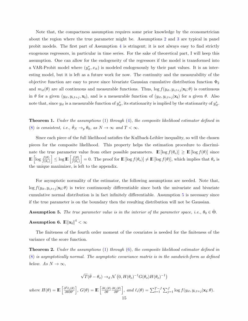
Theorem 1. Under the assumptions (1) through (4), the composite likelihood estimator defined in
(8) is consistent, i.e., θN →p θ0, as N →∞ and T <∞.
Since each piece of the full likelihood satisfies the Kullback-Leibler inequality, so will the chosen
pieces for the composite likelihood. This property helps the estimation procedure to discrimi-
nate the true parameter value from other possible parameters. IE [log f(θo)] ≥ IE [log f(θ)] since
IE[log f(θ)
f(θo)
]≤ log IE
[f(θ)f(θo)
]= 0. The proof for IE [log f(θo)] 6= IE [log f(θ)], which implies that θo is
the unique maximizer, is left to the appendix.
For asymptotic normality of the estimator, the following assumptions are needed. Note that,
log f(yit, yi,t+j |xi; θ) is twice continuously differentiable since both the univariate and bivariate
cumulative normal distribution is in fact infinitely differentiable. Assumption 5 is necessary since
if the true parameter is on the boundary then the resulting distribution will not be Gaussian.
Assumption 5. The true parameter value is in the interior of the parameter space, i.e., θ0 ∈ Θ.
Assumption 6. IE‖xi‖4 <∞
The finiteness of the fourth order moment of the covariates is needed for the finiteness of the
variance of the score function.
Theorem 2. Under the assumptions (1) through (6), the composite likelihood estimator defined in
(8) is asymptotically normal. The asymptotic covariance matrix is in the sandwich-form as defined
below. As N →∞,
√T (θ − θo)→d N
(0, H(θo)
−1G(θo)H(θo)−1)
where H(θ) = IE[∂2`i(θ)∂θ∂θ′
], G(θ) = IE
[∂`i(θ)∂θ
∂`i(θ)∂θ′
], and `i(θ) =
∑T−Jt=1
∑Jj=1 log f(yit, yi,t+j |xi; θ).
15

The asymptotic theory on the CL estimator in AR-Probit model, conceptually, is not differ-
ent than the asymptotic theory on pseudo-likelihoods (or quasi-likelihoods). However, the dif-
ficulty arises due to the nonlinearity in the parameters. The cumulative distribution function
Φ is not the only source of the nonlinearity; the function mit is also nonlinear in parameters –
especially in ρ. This ‘double’ nonlinearity result in complicated derivative functions of the com-
posite likelihood. Hence, computing the derivatives and finding bounds for them become non-
trivial. Despite this extra nonlinearity, the moment conditions on the process xt is not different
than those in static model, thanks to the assumption |ρ| < 1. For instance, the finiteness of
|∑∞
k=0 ρkβ′xt−k| ≤
∑∞k=0|ρ|
k‖β‖‖xt−k‖ in expectation is simply implied by the finiteness of ‖xt‖in expectation since |ρ| < 1. The complications and the nonlinearity of the model disappear when
ρ = 0. Thus, at any point in the proof, one can recover the conditions for static probit by imposing
ρ = 0.
Finally, in order to compute consistent estimator of the asymptotic covariance matrix, I intro-
duce consistent estimators for H(θ0) and G(θ0). They are
H(θN ) =1
N
N∑i=1
T−J∑t=1
J∑j=1
∂2 log f(yit, yi,t+j |xi; θN )
∂θ∂θ′
G(θN ) =1
N
N∑i=1
T−J∑t=1
J∑j=1
∂ log f(yit, yi,t+j |xi; θN )
∂θ
T−J∑t=1
J∑j=1
∂ log f(yit, yi,t+j |xi; θN )
∂θ
′
where the derivatives of the likelihood function are
∂ log f(yit, yi,t+j |xi; θN )
∂θ=
1∑s1=0
1∑s2=0
1s1,s2
∂∂θPs1,s2(θN )
Ps1,s2(θN )
∂2 log f(yit, yi,t+j |xi; θN )
∂θ∂θ′=
1∑s1=0
1∑s2=0
1s1,s2
Ps1,s2(θN )
[∂2Ps1,s2(θN )
∂θ∂θ′− 1
Ps1,s2(θN )
∂Ps1,s2(θN )
∂θ
∂Ps1,s2(θN )
∂θ′
]
Here the notation is simplified and the dependencies on (i, t, j) are suppressed. Clearly, 1s1,s2 de-
notes 1(yit = s1, yi,t+j = s2), and Ps1,s2(θ) denotes P (yit = s1, yi,t+j = s2 | xi; θ). More details on
the derivatives of the probability functions are given in the appendix.
A small note on choosing the lag length is worth to mention. As in the MLE case, one can
use AIC/BIC type of criteria to choose the lag length J in an optimal way. The criteria are in
their usual forms as in the pseudo-likelihood or quasi-likelihood estimation cases: AIC(θN ) =
−2Lc(θN |x, y)+2 tr{G(θN )H(θN )−1} and BIC(θN ) = −2Lc(θN |x, y)+log(N) tr{G(θN )H(θN )−1}.In theory, the larger is the lag length J the more efficient is the estimator; however, in practice
16

with finite N and T , sometimes larger J might bring less efficiency after some point due to the fact
that there might not be any useful information left after a certain J , and including these terms
in the composite likelihood might create extra noise (see Varin and Vidoni [2006] for a simulation
exercise in a time series setting). The same is true with the pairwise f(yit, yi,t+j) vs the triplet
f(yit, yi,t+j , yi,t+j+k) composite likelihood. The triplet composite likelihood is, in theory, more effi-
cient than the pairwise likelihood. However, in practice with finite data application, the (j+k)th lag
might just bring noise instead of useful information; moreover, it increases computational burden
exponentially.
There is nothing particular about large N fixed T setup of the composite likelihood in this paper.
Composite likelihood approach to AR-Probit model can also be used in a univariate time series
setting with N = 1 and large T , as well as in a large N large T panel setting. The identification
conditions and the derivatives of the bivariate probabilities will not be affected by any of these
changes. Certain moment conditions should be adjusted to provide the finiteness of the composite
likelihood and the hessian. Extra attention should be paid to the variance of G(θ0) matrix since
the terms in the score function will be correlated. Therefore, one needs to compute the long-run
variance when computing G(θ0). Thus, its estimator should utilize Newey-West type of long-run
variance estimator.
3.1.1 Comparison of CLE to GMM
As mentioned in the introduction, CLE and GMM resemble each other in the sense that pieces of
likelihoods are chosen for CLE whereas moments are chosen for GMM. They both require a choice
by the researcher. Theoretically, GMM is a more general estimation technique since it assumes
CLE as a special case where one can choose the moments as the score of the CLE. In this case,
CLE will be identical to GMM. In this section, I will compare pairwise CLE and GMM where the
most obvious and common moments are chosen. The simulation setup will mimic the setup of the
empirical part of this paper. In particular, I will argue that in a large N and moderate T panel
setting, GMM is inferior to CLE in terms of estimation performance as well as computation time.
The problem with GMM is that there are too many moments when T is not small, which makes
the computation of the efficient GMM infeasible.
Before showing the simulation result, let’s first analyze the moments for the GMM.
IE[yit|xi] = P(yit = 1|xi) = Φ(−mit)
Var[yit|xi] = Φ(−mit)Φ(mit)
IE[yityi,t+j |xi] = P(yit = 1, yi,t+j = 1|xi) = 1−Φ(mit)−Φ(mi,t+j) + Φ2
(mit,mi,t+j
∣∣ ρj)17

Let’s count the number of moments implied in each moment condition. For a K-dimensional co-
variate vector xit, the condition IE [{yit −Φ(−mit)}xit] = 0 for all t gives TK-many moments. The
moment condition for the variance IE[{
[yit −Φ(−mit)]2 −Φ(−mit)Φ(mit)
}xit]
= 0 for all t implies
also TK-many moments. Finally, IE[{yityi,t+j − 1 + Φ(mit) + Φ(mi,t+j)−Φ2
(mit,mi,t+j
∣∣ ρj)}xit] =
0 for all t and all j yields∑J
j=1(T − j)K-many moments. All in all, just by using the mean, vari-
ance, and covariance moments, we end up with TK +TK +∑J
j=1(T − j)K-many moments. In the
empirical study of this paper, N = 516, T = 55, J = 8, and K = 11. The number of moments in
such a setup would be 5654. To compute the efficient GMM, one needs to invert (5654 × 5654)-
dimensional weighting matrix, which is practically impossible. Thus, the second best thing one can
do is to invert the diagonal (5654×5654)-dimensional weighting matrix, which weights each moment
inversely according to its noise level. For the simulation purposes, I choose a smaller setup than
the empirical study of the paper. In the simulations, (N,T, J,K) = (500, 50, 4, 3) which implies
870 moments. Table 1 shows the simulation results. In this table, GMM indicates the first step
GMM with the identity matrix as the weighting matrix. Hence, it can be considered nonlinear least
squares estimation. E-GMM represents the second step GMM where the weighting matrix is the
inverse of the variances of each moment computed in the first step. Thus, it can be considered
weighted nonlinear least squares. Note that, the efficient GMM is not feasible since one needs to
invert a (870× 870)-dimensional matrix. The simulation study consists of 200 simulations.
The simulations clearly indicate that composite likelihood estimator outperforms GMM estima-
tor in this setup. The estimation of the autocorrelation parameter ρ is very accurate with CLE.
Moreover, the root mean squared errors (RMSE) are smaller for CLE except for one parameter. In
terms of computation times, CLE is around 100 times faster than GMM in a personal computer.
Naturally, this comparison can change from computer to computer, or might depend on the coding;
but, the computational attractiveness of CLE will stay intact.
[Figure 1 here]
4 Large N Moderate T Application: Credit Ratings
4.1 Introduction
Credit ratings reflect the creditworthiness of a borrower or obligor. Hence, they constitute an es-
sential part of investors’ decision of buying a company’s bonds – even its stocks. The accuracy and
timeliness of the ratings are important for the financial markets and the economy. Inaccurate or
miss-timed ratings can aggravate a crisis (Ferri et al. [1999]). Therefore it is important to correctly
18

model credit ratings. A part of credit risk modeling literature goes back to Altman [1968] where
corporate failure is analyzed by discriminant analysis based on accounting ratios (Altman Z-score
models). Since then, there have been numerous papers on credit scoring. However, these firm-level
models have been criticized for being static and missing the dynamic nature of the ratings. In this
paper, I propose a novel model for the credit rating literature: a panel autoregressive ordered probit
which takes into account the persistence of credit ratings, firm-specific variables, and the business
cycle. In this model, the observed discrete variable yit will represent the rating that firm i at time
t receives. The latent variable y∗it can be seen in different ways: y∗it is the continuous rating that
the firm gets during the creditworthiness assessment. Since the rating agency cannot publish a
continuous rating, they discretize these ratings and publishes letter grades. Another interpretation
can be the creditworthiness of the firm estimated by the rating agency. If this estimate falls between
certain threshold, then the firm is assigned a letter grade according to the interval it belongs to. All
in all, the latent variable reflects the view of the rating agency regarding the firm. In the model,
the persistence of the ratings is driven by the autocorrelation in the unobserved credit quality of
the firm as seen from the credit rating agency’s perspective, which depends on the firm’s financial
ratios and the state of the economy. Since the credit quality of a firm, in general, changes slowly,
the assigned ratings change slowly as a result. Moreover, because of the complicated nature of the
model, maximum likelihood estimation is impractical; thus, I use composite likelihood estimation
to estimate the model. The results show a small improvement over the static probit model for in-
sample predictions, but large improvements for pseudo out-of-sample predictions and the estimated
transition matrices. The dynamic nature of the model helps estimate the transition much more
successfully than the static model.
Investors might want to keep the risk level of their portfolio at a certain level. Since re-balancing
a portfolio is costly, investors prefer rating stability rather than ratings to reflect temporary changes
in companies’ financial conditions. At the same time, ratings should reflect an accurate estimate of
the borrower’s condition. Hence, timeliness of ratings is also important. In this regard, credit rating
agencies face a trade-off between rating stability and accuracy (Cantor and Mann [2006]). There
are two conceptual approaches for assigning ratings: Through-the-cycle (TTC) and Point-in-time
(PIT). TTC (also called cycle-neutral) methodology focuses more on the permanent component
of default risk rather than short-term fluctuations due to business cycles. Hence, TTC approach
renders ratings more stable and rating migration more prudent. However, with this methodology,
the timeliness of the ratings can be at question since ratings might lag the actual default risk of
a company. In PIT method, on the other hand, current conditions of a company has a big effect
on its credit rating. With this approach, ratings predominantly reflect the current condition of the
borrower. The question of whether credit rating agencies assign ratings according to TTC or PIT
has attracted a lot of attention from researchers. There are several papers providing evidence for
19

the pro-cyclical behavior of ratings. See, for instance, Nickell et al. [2000], Bangia et al. [2002],
Amato and Furfine [2004], Koopman and Lucas [2005], Feng et al. [2008], Topp and Perl [2010],
Auh [2015], and Freitag [2015]. Some of these papers conclude that this is evidence for PIT rat-
ings. However, rating actions being pro-cyclical does not necessarily imply that the ratings reflect
short-term fluctuations. For instance, during a recession, there might be a significant change in the
long-term credit quality of a firm. Therefore, lower ratings during a recession do not mean that the
rating agencies cannot see through the cycle. On the TTC side of the literature, Loffler [2004, 2013]
and Kiff et al. [2013] show that the credit ratings have predictive power on the long-term component
on default probabilities. The slow and delayed reaction by credit rating agencies are empirically
documented by Altman and Rijken [2006] and Loffler [2005]. The empirical results in this paper
support this phenomenon, thus provide evidence for TTC ratings. In particular, the results show
that at the beginning of Great Recession, the rating agencies waited 2-3 quarters before reflecting
the changes in the credit quality of the firms on their ratings. This finding is quantitatively in line
with the estimates in Altman and Rijken [2006]. They find that the TTC methodology delays the
timing of rating migrations by 0.70 year on average.
[Figure 1 here]
Cheng and Neamtiu [2009] described the rating quality by three properties: accuracy, stability
(or volatility), and timeliness. In this paper, I focus on the stability of the ratings. TTC methodol-
ogy is designed to induce rating stability (Carey and Hrycay [2001]). However, little research is done
on quantifying the stability of the credit ratings. One way of inferring rating stability is through
the frequency of rating transitions. Smaller transition frequencies mean higher stability. Figure 1
displays percentage of issuers for which their ratings stayed unchanged from one year to another.
For instance, the highest stability in the ratings occurred in the year 2004 – more than 75% of the
firms stayed in the same rating class. On the other hand, the lowest stability occurred during the
Great Recession. Motivated by this observation, the rating stability can be measured through the
diagonal (and near diagonal) elements of a transition matrix. The diagonal element of a transition
matrix shows the percentage of firms that stayed in the same rating class in a given year. Jafry
and Schuermann [2004] and Amato et al. [2013] generate “mobility indices” by analyzing the sin-
gular values and the eigenvalues of the yearly rating transition matrices. These indices capture the
time-varying stability of ratings over the years. But, these values are obtained without controlling
for any firm or macroeconomic conditions. In this regard, these indices represent the unconditional
stability of the ratings. There are also portfolio models that use transition matrices and control for
business cycle effects. However, these models are “cohort-style”, that is, all the firms within a rating
class are identical. Hence, the rating classes exhibit persistence and correlations among themselves
20

where individual firms actually do not matter. But, the research by Lando and Skødeberg [2002]
and Frydman and Schuermann [2008] shows that two firms with identical current credit ratings can
have substantially different transition probabilities. This shows that ratings exhibit non-Markovian
property. In this regard, AR-Probit model seems a better model to analyze the ratings since the
ordered outcome variable in this model is non-Markovian. Moreover, the analysis is done at the
firm level by controlling for firm balance sheet ratios and business cycle variables. Finally, the
rating stability is inferred by the autocorrelation parameter (ρ) of the underlying continuous latent
variable. Hence, the stability is induced from the fundamentals of a firm. The higher is ρ the higher
is the stability of ratings. Moreover, the model can be extended to a time-varying parameter model,
where the rating stability can be estimated at a quarterly level.
In Dynamic Probit model, last period’s credit rating yi,t−1 is used to predict the current one yit.
Mizen and Tsoukas [2009] use this model for forecasting purposes. As they noted, the knowledge
of the previous rating helps the forecast but the coefficients of yi,t−1 do not say anything about
persistence, instead, it just shifts the latent credit quality of the firm by constant term. Note
that, the right-hand-side variable yi,t−1 actually represents a dummy variable for each rating class.
Consider a firm with a high rating, say AAA. There is no upper level ratings that a AAA firm
can go to; such firms can face only downgrades. Therefore, a AAA rating in the previous period
will necessarily render the coefficient of yi,t−1 to be negative. A similar argument will be valid for
AA firms as well since it is more likely for a AA firm to face a downgrade than an upgrade. From
the opposite angle, firms that are below investment grade will be more likely to have upgrades –
especially if the data do not include default observations. Thus, the most likely direction for a
speculative grade is upwards, which renders the coefficient of previous BB/B/CCC rating to be
positive. All in all, the coefficients of the previous rating artificially captures the convergence to
the middle rating BBB instead of capturing the stability. The assigned ratings should be a result
of the unobserved creditworthiness of a firm, not a determinant of it.
The empirical analysis focuses on three parts. The first part is a comparison of static probit
model and AR-Probit model. The estimation results show a significant and economically large
persistent parameter. In AR-Probit, one can compute short-term and long-term effects of the
explanatory variables. In static model, however, the effects last only one term. In comparison, I
find that the estimates from the static model are indeed an average between the short-term and long-
term cumulative effects computed from AR-Probit estimates. In particular, static model estimates
are close to the 2-to-4 quarter cumulative effects derived from AR-Probit model. Regarding in-
sample prediction performances, both model performs similarly – though AR-Probit model has a
better prediction for infrequent rating classes. Regarding transition matrix estimates, AR-Probit
model shows 5 times better performance than the static model since it accounts for persistence in
21

the ratings. In the second part, time-varying parameter model is utilized to estimate changes in the
rating stability over time. The results show that the stability declines over time. But, the decline
is more prominent after the crisis. It means that the rating agencies try to assign the ratings more
timely. One reason for that can be the critics on rating agencies during the recession. Another one
is the new regulations enforced on the agencies to increase their liability. Trying to increase the
rating quality after critics and regulations are in line with the findings in the literature (see Cheng
and Neamtiu [2009]). Facing widespread criticism, the credit rating agencies might be concerned
for their reputation and start assigning the ratings more conservatively. In the third part, I show
the evidence for sluggish rating adjustment during the recent crisis. Based on the time-varying
parameter model, the results show that the credit rating agencies increase the weights on the past
information – to keep the ratings stable – when they face changes in the financial situation of the
firm.
4.2 Data
I use Financial Ratios Suite by WRDS database for quarterly balance sheet financial ratios of com-
panies. The measure of credit rating is the S&P Long-Term Issuer Level rating obtained from Com-
pustat in WRDS database. Ratings are available in monthly frequency; I convert them to quarterly
frequency by taking the last rating within each quarter assuming that the most up-to-date informa-
tion on a firm is contained in the most recent rating. Firm-level data are between 2002Q1-2015Q3.
I use the quarterly macro data set of McCracken and Ng [2015] to extract business cycle factors.
The factors are estimated by principal component analysis from a large panel of macro variables
that include real sector, employment, housing, prices, interest rates, money and credit, exchange
rates, and financial data. In the data set, there are in total 218 variables between 1971Q2–2015Q3.
After extracting two principal components with the largest eigenvalues, I took the corresponding
dates of the factors that match with the data range of credit ratings. Hence, the estimated factors
capture the business cycle of the economy. Finally, NBER recession dates are obtained from FRED.
Even though the term “credit rating of a firm” is frequently used, the corporate bond that is
issued by the obligor receives a rating, rather than the obligor itself. An obligor can issue several
bonds, and each issue might have a different rating. However, senior unsecured long-term bonds’
rating are close to the issuer rating since the debt defaults only when the issuer defaults. There-
fore, Long-Term Issuer Level ratings are de-facto the creditworthiness of the obligor. I convert
letter ratings into ordinal numbers from 1 to 7 corresponding to the grades {CCC, B, BB, BBB,
A, AA, AAA}, respectively, that is CCC=1 and AAA=7. Note that, I grouped ratings without
considering notches +/−, e.g., AA−, AA and AA+ belong to a single category denoted as AA.
The CCC category contains all the ratings including any C letter, i.e., CCC+, CCC, CCC−, CC,
and C. Observations with D, SD (Suspended) or NM (Not meaningful) ratings are excluded. In the
22

robustness analyses, defaulted firms will also be included in the dataset.
Using financial ratios for credit rating determination in discrete choice models is common in
the literature. I do not claim that this is the exact method the credit rating agencies do follow to
generate the ratings. Yet, as described in Van Gestel et al. [2007], the real rating process may be
well approximated by such models with financial ratios as determinants. Moreover, Standard and
Poor’s [2013] gave a list of Key Financial Ratios that are used in rating adjustment process. One
thing to note is that some financial ratios are highly correlated with each other, thus one needs to
take this into account while choosing the variables. Another important thing is that some ratios are
not available at a quarterly frequency. Based on these criteria, I use the following set of financial
ratios that capture solvency, financial soundness, profitability, and valuation of a firm: total debt
leverage (debt/assets), long-term debt to total debt ratio (ltd/debt), return on assets (roa), cover-
age ratio (cash/debt), net profit margin, and valuation ratio (price/sales). The detailed definitions
and descriptive statistics of the variables are given in Table 2 and Table 3, respectively.
[Table 2 here]
[Table 3 here]
As a solvency measure, the debt-to-asset ratio is used, which reflects the leverage level of the
firm. In general, the higher is this ratio the riskier is the company in terms of meeting its debt
payments. Financial soundness is implied by the ratios of total long-term debt to total debt 6
and operating cash flow to debt. The former ratio shows the capital structure of the firm and is
negatively related to credit ratings whereas the latter one is a coverage ratio showing the ability to
carry the debt of the company and is positively related to credit ratings. Profitability is another
important aspect showing how easy a firm can generate income. It is captured by return on assets
and net profit margin 7 , which are positively correlated to credit ratings. Finally, as a valuation
ratio, I use market value to sales ratio8.
6In the literature, many papers use the ratios debt-to-assets and long term debt to assets together in regressions.However, these variables are highly correlated (∼ 75%). To avoid multicollinearity, I prefer using long term debt tototal debt ratio to capture the debt structure instead of long term debt to assets.
7Operating profit margin (opm) is more frequently used than net profit margin (npm) in the literature. However,Corr(roa, opm) = 0.84, but Corr(roa, npm) = 0.64. It means that {roa, opm} is likely to create multicollinearityproblem whereas {roa, opm} is not. Moreover, given the fact that Corr(opm, npm) = 0.76 and that opm and npmhave very similar definitions, I choose nmp over opm for the analysis.
8Many papers use price-to-book ratio instead of price-to-sales. However, these papers have annual data. But, atthe quarterly frequency the data for p/b have a lot of missing values. Another famous choice is price-to-earnings ratio.However, especially during the crises many firms suffer losses, i.e., they do not make any earnings, which renders p/e
23

To control for the state of the economy, the literature uses various choices of business cycle
variables. The NBER recession dummy seems the most common choice, but choice of macro funda-
mental variables differ from paper to paper. While some papers use GDP growth rate (Feng et al.
[2008], Koopman et al. [2009], and Alp [2013]), others create their business cycle indicator (Amato
and Furfine [2004], Freitag [2015]). Hence, it is not clear which business cycle variable should be
used. For this reason, I prefer using estimated factors from a large macroeconomic data set. The
first two principal components (called Factor1 and Factor2) explain more than 20% of the total
variation in 218 business cycle variables. They are especially related to the real economy sector.
For instance, they explain around 70% of the variation in real variables such as output, exports,
imports, personal income, private investment, and housing starts. These estimated factors appear
to be positively correlated with the ratings whereas the ratings are lower during the NBER recession
dates, as expected.
For the empirical baseline results, a balanced panel data set is used. In this data set, there are
516 firms over 55 quarters (2002Q1–2015Q3) with no missing data. Hence, they are the firms that
‘survived’ throughout the data period. The frequency of the ratings in this data set is given on
the left side of Table 4. Since more than 70% of the ratings are in the investment grade category,
we can consider this data set as investment-grade firms. As a robustness check, estimation results
based on an unbalanced panel data set are also presented. The reason why this data set is not
the baseline is two folds. First, it is not clear how to model D rated firms. Should the D ratings
be excluded from the analysis or do these observations indeed contain useful information in terms
of rating dynamics? Note that, a D rating does not necessarily mean that the firm is out of the
market. There are firms that have consecutive D ratings for a few quarters, but then continue being
rated without any interruption in their rating history9. Second, due to the autocorrelation in the
latent variable, modeling the missing data in the middle of a firm’s history is not straightforward;
it will result in a complex formulation. As a result, I include data for the firms that do not have
any missing data once they entered the market until they leave. A firm is allowed to enter the data
set after the initial date 2002Q1 and to leave it before 2015Q3. Since the firms with an extremely
short span of data are not representative and exhibit large variations, I excluded firms that have less
than 5 years of quarterly data. Moreover, D ratings are also included in the data set as long as the
balance sheet data are also available. Finally, there are 1406 firms with an average of 38 quarters in
this data set. The frequency of the ratings for the unbalanced panel data is given on the right side
ratio meaningless for a crucial period in the dataset. For these reasons, I prefer using price-to-sales ratio over p/band p/e.
9For instance, Xerium Technologies Inc. filed bankruptcy for 2010Q1–2010Q2, but was rated B in 2010Q3 andcontinued being in the market. As long as we can observe how the defaulted firms’ balance sheet data evolve, comingfrom bankruptcy back to business, in fact, contains useful information. Such cases are obviously rare (most firms’data ends once they default), and omitting them will not affect the estimates.
24
of Table 4. In this data set, ratings are more evenly distributed. In particular, we have a relatively
higher representation of sub-investment firms compared to the balanced panel. This difference will
allow us to highlight characteristic differences between investment and non-investment firms.
[Table 4 here]
4.3 Extensions of the Model
In this subsection, I extend the baseline model into various directions. All these models will be
used in the empirical part to address different aspects of the credit rating data. The first extension
is changing the binary response variable into an ordered one. This model will be the working
model of the empirical part. Another extension is allowing for random effects to control for firm
heterogeneity. Another interesting extension is allowing for time-varying parameters, in particular,
time-varying autocorrelation coefficient. Finally, I will analyze unbalanced panel probit model.
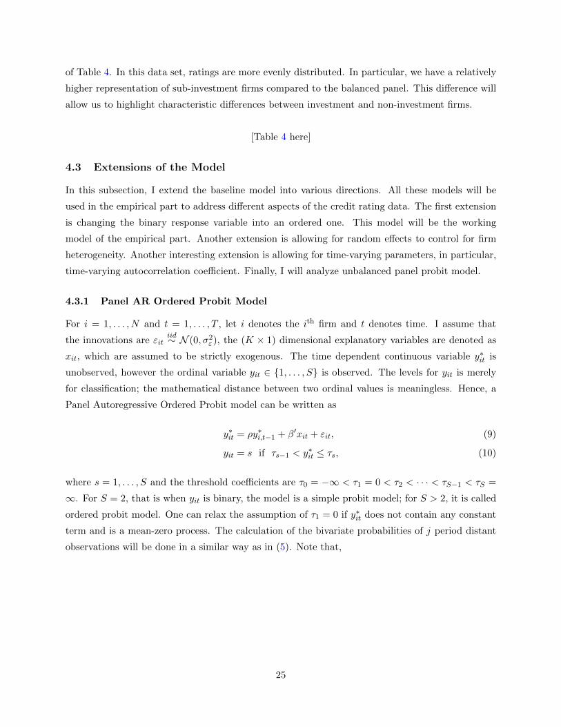
4.3.1 Panel AR Ordered Probit Model
For i = 1, . . . , N and t = 1, . . . , T , let i denotes the ith firm and t denotes time. I assume that
the innovations are εitiid∼ N (0, σ2
ε), the (K × 1) dimensional explanatory variables are denoted as
xit, which are assumed to be strictly exogenous. The time dependent continuous variable y∗it is
unobserved, however the ordinal variable yit ∈ {1, . . . , S} is observed. The levels for yit is merely
for classification; the mathematical distance between two ordinal values is meaningless. Hence, a
Panel Autoregressive Ordered Probit model can be written as
y∗it = ρy∗i,t−1 + β′xit + εit, (9)
yit = s if τs−1 < y∗it ≤ τs, (10)
where s = 1, . . . , S and the threshold coefficients are τ0 = −∞ < τ1 = 0 < τ2 < · · · < τS−1 < τS =
∞. For S = 2, that is when yit is binary, the model is a simple probit model; for S > 2, it is called
ordered probit model. One can relax the assumption of τ1 = 0 if y∗it does not contain any constant
term and is a mean-zero process. The calculation of the bivariate probabilities of j period distant
observations will be done in a similar way as in (5). Note that,
25
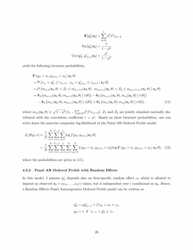
IE[y∗it|xi] =
t∑k=0
ρkβ′xi,t−k
Var[y∗it|xi] =1
1− ρ2
Cov[y∗it, y∗i,t+j |xi] =
ρj
1− ρ2,
yield the following bivariate probabilities.
P (yit = s1, yi,t+j = s2 | xi; θ)
= P(τs1 < y∗it ≤ τs1+1, τs2 < y∗i,t+j ≤ τs2+1 | xi; θ
)= P
(ms1,t(xi, θ) < Z1 ≤ ms1+1,t(xi, θ), ms2,t+j(xi, θ) < Z2 ≤ ms2+1,t+j(xi, θ)
∣∣ xi; θ)
= Φ2
(ms1+1(xi, θ),ms2+1(xi, θ)
∣∣ r(θ))− Φ2
(ms1+1(xi, θ),ms2(xi, θ)
∣∣ r(θ))− Φ2
(ms1(xi, θ),ms2+1(xi, θ)
∣∣ r(θ))+ Φ2
(ms1(xi, θ),ms2(xi, θ)
∣∣ r(θ)) , (11)
where ms,t(xi, θ) ≡√
1− ρ2(τs −
∑tk=0 ρ
kβ′xi,t−k), Z1 and Z2 are jointly standard normally dis-
tributed with the correlation coefficient r = ρj . Based on these bivariate probabilities, one can
write down the pairwise composite log-likelihood of the Panel AR Ordered Probit model.
Lc(θ|y, x) =1
N
N∑i=1
T−J∑t=1
J∑j=1
log f(yit, yi,t+j |xi; θ)
=1
N
N∑i=1
T−J∑t=1
J∑j=1
S∑s1=1
S∑s2=1
1(yit = s1, yi,t+j = s2) logP (yit = s1, yi,t+j = s2 | xi; θ) , (12)
where the probabilities are given in (11).
4.3.2 Panel AR Ordered Probit with Random Effects
In this model, I assume y∗it depends also on firm-specific random effect αi which is allowed to
depend on observed xi = (xi1, . . . , xiT ) values, but is independent over i conditional on xi. Hence,
a Random Effects Panel Autoregressive Ordered Probit model can be written as
y∗it = ρy∗i,t−1 + β′xit + αi + εit,
yit = s if τs−1 < y∗it ≤ τs,
26

The firm-specific random effects will capture the effects that change over firms but not over time. For
instance, it is likely to capture the location of the firm, the sector the firm is operating in, managerial
activities, etc. as long as these variables do not change over time. Otherwise, they will be captured
by idiosyncratic shocks εitiid∼ N (0, σ2
ε). One cannot treat the unobserved firm heterogeneity as fixed
effects and estimate them as parameters due to incidental parameter problem; it will yield biased
and inconsistent estimates. There are a couple of ways to deal with the unobserved random αi: it
can be integrated out or replaced by a reduced form equation. In either way, one needs to make a
distributional assumption for αi, say αiiid∼ N (γo + γ′1xi, σ
2α) where xi is the average of xit over t.
For identification purposes, we need to put a restriction on the variances of the innovations. The
following will be assumed for the random effects model σ2α + σ2
ε = 1. Note that, the parameter θ in
this model also contains the extra parameters arising due to random effects, that is, (γo, γ′1, σ
2α, σ
2ε).
The first approach will yield a likelihood function containing a one-dimensional integral, which can
be approximated as accurately as desired by Gauss–Hermite quadrature 10.
Lθ|y,x) =N∏i=1
∫f(yi|xi, αi)φ
(αi|γo + γ′1xi, σ
2α
)dαi
=N∏i=1
1√π
G∑g=1
wgf(yi
∣∣∣ xi, (√
2σαHg + γo + γ′1xi))
where φ(z|µ, σ2) denotes the normal probability density with mean µ and variance σ2 evaluated
at z, the nodes Hg are the zeros of gth order Hermite polynomial, and wg are the corresponding
weights. Hence,∑G
g=1 approximates the integral by evaluating the function f at specific nodes and
then weighting them. The pairwise likelihood of f(yi|xi, αi) can be computed in the exactly same
way as in (12), where αi will be replaced by normalized nodes√
2σαHg + γo + γ′1xi.
In the other approach, αi is replaced by a reduced form equation. Let’s assume that y∗i0 =
β′xi0 + 11−ραi + 1√
1−ρ2εi0 where εi0
iid∼ N (0, σ2ε) and αi = µ + γ′xi + ηi where ηi ∼ N (0, σ2
α) such
10Gauss–Hermite quadrature is used for numerical integration; it approximates a specific type of integral in thefollowing way. ∫ ∞
−∞h(x) exp(−x2)dx ∼=
K∑k=1
wkh(xk),
where the nodes xk are zeros of kth order Hermite polynomial and wk are corresponding weights. A table for thenodes and the weights can be found in Abramowitz et al. [1972], page 924. If one has a normal density instead ofexp(−x2), a standardization will be needed.∫ ∞
−∞h(x) exp(−0.5(x− µ)2/σ2)dx =
∫ ∞−∞
h(√
2σx+ µ) exp(−x2)dx ∼=K∑k=1
wkh(√
2σxk + µ).
27

that σ2α + σ2
ε = 1.
y∗it = ρy∗i,t−1 + β′xit + αi + εit
= ρty∗i0 +
t−1∑k=0
ρkβ′xi,t−k +1− ρt
1− ραi +
t−1∑k=0
ρkεi,t−k
=t∑
k=0
ρkβ′xi,t−k +1
1− ραi +
ρt√1− ρ2
εi0 +t−1∑k=0
ρkεi,t−k
=µ
1− ρ+
γ′
1− ρxi +
t∑k=0
ρkβ′xi,t−k +1
1− ρηi +
ρt√1− ρ2
εi0 +t−1∑k=0
ρkεi,t−k
The presence of ηi generates autocorrelation in the composite error term ηi + εit, which needs to
be taken into account in calculating bivariate probabilities and the correlation coefficients. The
following statistics will be used in the bivariate probabilities.
IE[y∗it|x] =µ
1− ρ+
γ′
1− ρxi +
t∑k=0
ρkβ′xi,t−k
Var[y∗it|x] =σ2α
(1− ρ)2+
σ2ε
1− ρ2(13)
Cov[y∗it, y∗i,t+j |x] =
σ2α
(1− ρ)2+
ρjσ2ε
1− ρ2
Corr[y∗it, y∗i,t+j |x] =
σ2α
(1−ρ)2+ ρjσ2
ε1−ρ2
σ2α
(1−ρ)2+ σ2
ε1−ρ2
(14)
This correlation formula looks complicated, however, note that if there was no firm heterogeneity,
i.e., if σ2α = 0, then the correlation becomes ρj , as it was the case in Panel AR-Probit model in
(11). If there was no idiosyncratic variation, i.e., σ2ε = 0, then the correlation becomes 1 since the
persistence in the composite error does not diminish due to the presence of ηi for each t. Hence, the
correlation formula above represents the weighted average of these two extreme case correlations.
Based on this correlation coefficient, one can say that in Panel AR-Probit models the interpretation
of ρ is different depending on the presence of random effects. In models without random effects,
ρ solely controls the autocorrelation of the latent state variable y∗it. In contrast, when the firm-
specific random effects exist, ρ is not the only source of persistence because αi also persists over
time thereby adds to the persistence of the latent process.
Denoting xit = (x′it, 1, x′i)′, δ = (β′, µ, γ′1)′, and using backwards substitution on y∗it gives let us
28
compute the bivariate probabilities as follows.
P (yit = s1, yi,t+j = s2 | xi; θ)
= P(τs1 < y∗it ≤ τs1+1, τs2 < y∗i,t+j ≤ τs2+1 | xi; θ
)= P
(ms1,t(xi, θ) < Z1 ≤ ms1+1,t(xi, θ), ms2,t+j(xi, θ) < Z2 ≤ ms2+1,t+j(xi, θ)
∣∣ xi; θ), (15)
where ms,t(xi, θ) ≡√
σ2α
(1−ρ)2+ σ2
ε1−ρ2
(τs − µ
1−ρ −γ′
1−ρ xi −∑t
k=0 ρkβ′xi,t−k
), Z1 and Z2 are jointly
standard normally distributed with the correlation coefficient given in (14). As a result, this ap-
proach resembles the basic model defined in (9)-(10) except that now the errors are allowed to be
autocorrelated with a special structure and that the regressors contain time averages. Therefore,
the pairwise log-likelihood of this model will resemble that in (12) with a more complicated bivariate
probability structure taking into account the extra autocorrelation in the errors.
4.3.3 Panel AR Ordered Probit with Time-Varying Coefficients
In this section, I allow the parameters to change over time – in particular the persistence parameter
ρ. Especially in credit ratings application, time-varying persistence will be important to see how
rating stability changes over time. This will give us some idea whether credit rating agencies assign
their ratings according to the business cycle. In other words, it will indicate whether credit rating
agencies use TIC or PIT approach. Moreover, we can also see whether policy changes, like Dodd–
Frank Act, have any effect on rating stability. The model with time-varying persistence can be
written as
y∗it = ρty∗i,t−1 + β′xit + εit, (16)
yit = s if τs−1 < y∗it ≤ τs, (17)
Let’s assume that y∗i0 = β′xi0 + εi0 where εi0iid∼ N (0, 1) (note that, if y∗i0 = 0 is assumed then ρ1
cannot be estimated). Let’s denote the new parameter vector as θ = (ρ1, . . . , ρT , β′, τ ′)′. A sufficient
condition for a non-explosive behavior of y∗it is |ρt| < 1 for all t. Time-varying parameters will be
identified from the cross-section variation. In other words, information on ρt will be accumulated
by the rating changes of the firms between periods (t − 1) and t. In this model, again backward
substitution will be used, but the time-varying parameters will complicate the bivariate probabilities
29

in terms of parameters.
y∗i1 = ρ1y∗i0 + β′xi1 + εi1
y∗i2 = ρ2y∗i1 + β′xi2 + εi2 = ρ2ρ1y
∗i0 + β′xi2 + ρ2β
′xi1 + εi2 + ρ2xεi1
...
y∗it =
(t∏
k=1
ρk
)y∗i0 + β′xit +
t∑k=2
(t∏
s=k
ρs
)β′xi,k−1 + εit +
t∑k=2
(t∏
s=k
ρs
)εi,k−1
= β′xit +
t∑k=1
(t∏
s=k
ρs
)β′xi,k−1 + εit +
t∑k=1
(t∏
s=k
ρs
)εi,k−1
The following statistics will be used in computing the bivariate probabilities.
IE[y∗it|x] = β′xit +
t∑k=1
(t∏
s=k
ρs
)β′xi,k−1
Var[y∗it|x] = 1 +
t∑k=1
t∏s=k
ρ2s
Cov[y∗it, y∗i,t+j |x] =
(t+j∏
s=t+1
ρs
)[1 +
t∑k=1
t∏s=k
ρ2s
]
Corr[y∗it, y∗i,t+j |x] =
(t+j∏
s=t+1
ρs
)√1 +
∑tk=1
∏ts=k ρ
2s
1 +∑t+j
k=1
∏t+js=k ρ
2s
(18)
As t gets larger, the term inside the square root will be very close to 1. Thus, the correlation
between accumulated discounted errors can be approximated by∏t+j−1s=t ρs+1. This is also the
correlation between y∗it and y∗i,t+j conditional on xi. If all the persistence parameters are the same
ρt = ρ, then the correlation coefficient simply becomes ρj as t gets larger, as in the baseline Panel
AR-Probit case. The bivariate probabilities of the pair (yit, yi,t+j) in this model can be computed
in the following way.
P (yit = s1, yi,t+j = s2 | xi; θ)
= P(τs1 < y∗it ≤ τs1+1, τs2 < y∗i,t+j ≤ τs2+1 | xi; θ
)= P
(τs1 < β′xit +
t−1∑k=1
(t−1∏s=k
ρs+1
)β′xik + εit +
t−1∑k=1
(t−1∏s=k
ρs+1
)εik ≤ τs1+1,
τs2 < β′xi,t+j +
t+j−1∑k=1
(t+j−1∏s=k
ρs+1
)β′xik + εi,t+j +
t+j−1∑k=1
(t+j−1∏s=k
ρs+1
)εik ≤ τs1+1 ≤ τs2+1
∣∣∣∣∣ xi; θ
)
= P
(ms1,t(xi, θ) < Zit ≤ ms1+1,t(xi, θ), ms2,t+j(xi, θ) < Zi,t+j ≤ ms2+1,t+j(xi, θ)
∣∣∣∣∣ xi; θ
), (19)
30

where
ms,t(xi, θ) ≡τs − β′xit −
∑t−1k=1
(∏t−1s=k ρs+1
)β′xik√
1 +∑t−1
k=1
∏t−1s=k ρ
2s+1
and Zit ≡εit +
∑t−1k=1
(∏t−1s=k ρs+1
)εik√
1 +∑t−1
k=1
∏t−1s=k ρ
2s+1
,
Zit and Zi,t+j are jointly normally distributed with zero mean, unit variance, with the correlation
coefficient given in the equation (18). Hence, the pairwise log-likelihood is the same as in (12)
except that the parameter vector now contains {ρt}Tt=2 and the probabilities are given in (19).
4.3.4 Unbalanced Panel AR-Probit
I allow missing values. CL allows any part of the likelihood. Hence, the likelihood of only observed
data will be included. That is, the likelihood of a firm with available data between ti and Ti will
contribute to the composite likelihood. For simplicity, I assume that there is no missing observation
once the data for a firm started. However, a firm may enter the market after the initial date
of data or may leave the market before the end date. Hence, 1 ≤ ti < Ti ≤ T for all i. The
backwards substitution (4) of the state variable for firm i is done for the available observations, i.e.,
for t = ti, . . . , Ti. Similarly for the bivariate probabilities. Hence, the pairwise log-likelihood of the
data including missing values is
Lc(θ|y,x) =1
N
N∑i=1
log f(yi|xi; θ)
=1
N
N∑i=1
Ti−J∑t=ti
J∑j=1
log f(yit, yi,t+j |xi; θ)
=1
N
N∑i=1
Ti−J∑t=ti
J∑j=1
S∑s1=1
S∑s2=1
1(yit = s1, yi,t+j = s2) logP (yit = s1, yi,t+j = s2 | xi; θ) ,
(20)
where ti is the initial date with available observation for firm i, and Ti is the date when the available
observations for firm i ends. I assume between ti and Ti, there is no missing values. In theory,
one can allow for missing observations even between ti and Ti, however, modeling the persistence
in an autoregressive setting with missing values in-between the observations would be extremely
complicated.
4.4 Empirical Results
In this section, I compare the estimation results of static probit and AR-Probit models estimated
by maximum likelihood and composite likelihood, respectively. Table 5 shows the estimates of the
models. In the table, for both static and autoregressive model, the signs of financial ratios and
31
business cycle variables are the same. Moreover, the signs are as expected a priori, except for
cash/debt. The sign of cash related variables is estimated to be negative in many other papers
in the literature, see for example Alp [2013]. This puzzling phenomenon is explained by Acharya
et al. [2012] by observing that firms tend to have high cash holdings for precautionary motive.
In-sample prediction accuracy seems slightly higher for static model compared to AR model (47%
vs. 44% correctly estimated ratings). However, this measure of predictive performance can be
greatly affected when there is a dominant outcome in the data. The correct prediction of each
rating class reveals that this higher prediction accuracy of the static model comes from predicting
accurately only the BBB rating class, which contains the largest number of observations. On the
other hand, AR-Probit model yields more balanced correct prediction over rating classes. To avoid
this seemingly successful predictability, I also report the average of the correct predictions over each
rating class. This measure is in line with the technique proposed by Merton [1981] to distinguish
between true predictability and seemingly successful predictability of a ‘stopped-clock.’ Based on
the average correct prediction, AR-Probit model has a better prediction power overall (26% vs 22%).
The most important difference between the static and autoregressive models is, clearly, a sig-
nificant and economically large persistence parameter (ρ = 0.62), which indicates that there is, in
fact, a need for a time series component in analyzing credit ratings. A significant ρ shows that
the soundness of a company evaluated by the rating agency, represented by latent y∗it, measured
by its financial ratios and the current economic conditions exhibits significant persistence. Any
unexpected change in the rating agency’s view of the soundness of a firm has a half-life more than a
quarter. Even after a year, ρ4 = 15% of the shock is affecting the continuous rating of the firm. In
the static model, on the contrary, there is no difference between the short-term effect and the long-
term effect. Any change affects the current ratings and then disappears. Therefore, the estimates
of the static model reflect the “mid-term effect” of a shock. In particular, the estimates in the static
model is the closest to the 6-month cumulative effects derived from the AR-Probit estimates (see
Table 5).
[Table 5 here]
An important question is how a change in the unobserved state of the firm will be reflected in
its ratings. Due to nonlinearity in the model, it is hard to interpret the coefficients. The impact of
a shock on ratings depends on the current conditions of the firm. Considering the estimated thresh-
olds, (τ1, τ2, τ3, τ4, τ5, τ6) = (0, 1.2, 2.3, 3.6, 4.8, 5.8), the estimated average distance between the
rating categories is (τ6 − τ1)/5 = 1.17. Note that τ1 is set to be zero for identification purposes,
in particular, to identify the constant term in the measurement equation. One should also note
32

that this average distance is valid between the rating categories B–AA because the region for CCC
is (−∞, 0], and the region for AAA is (5.8,∞). Hence, focusing on the middle rating classes, on
average, a 1.17 units increase in the latent variable will result in a rating upgrade in the current
quarter. In reality, a letter grade change within a quarter is an extreme case, but it is still a useful
exercise to understand the dynamics of the model. Because of the persistence, the shock will also
have an effect on the state of the firm in the jth quarter after the shock by a magnitude of 1.17ρj .
In other words, in each quarter over a year, the effect of a shock with a magnitude 1.17 will be
(1.17, 0.73, 0.45, 0.28, 0.18), or in cumulative terms the effect will be (1.17, 1.9, 2.35, 2.63, 2.81).
It means that contemporaneously there is a rating upgrade by one letter, and one more increase
by the end of 6 months, and there are no upgrades afterward. However, note that I am using only
letter grades instead of notches; most ratings have +/- notches as an addition. Let’s assume that
the notches are evenly distributed between two thresholds. As a conclusion, this analysis shows
that, on average, a shock that increases a company’s credit rating contemporaneously by one letter
will result in a further increase in its rating by two notches in the following quarter, and another
notch increase in the second quarter, and one last notch increase in the fourth quarter, which re-
sults in a 2 letter and a notch increase by the end of the year. Hence, a full letter upgrade in a
quarter will have a momentum effect with another letter and a notch upgrade gradually within a
year. The shock that increases a firm’s rating by two letters and a notch within a year must be a
very large shock, which is a rare event clearly. But based on this exercise, more interpretable and
reasonable economic examples will be given below by using shocks to financial ratios and business
cycle variables.
Next, I will analyze the effect of a 1-year long recession on credit ratings. In each quarter during
the recession, the latent variable is down by the estimated coefficient of the recession βrec = −0.27.
Moreover, due to the persistence in y∗it, the negative effects of the previous periods are carried over
with exponentially decaying weights. If we divide this cumulative effect by the average rating dis-
tance, we obtain the normalized cumulative effect of a recession on letter grades. The cumulative
effect at the jth quarter is calculated simply by the formula βrec(1 + ρ + · · · + ρj)/(τ6/5). The
estimated effect of a recession on credit ratings for each quarter is (−0.23,−0.61,−1.07,−1.59).
The results imply that there is one letter and two notches decrease in the credit ratings by the
end of the year during a recession. If we apply the same idea to the financial ratios to see their
long-run effect after a one-time change by a magnitude of their one standard deviation, we obtain
the following results. In the long run, a one standard deviation change in the ratio of long-term
debt to liabilities has the highest impact on credit ratings, which is a downgrade by almost three
notches. The second highest impact occurs when the ratio of operating income before depreciation
to assets, which reflects profitability, increases by one standard deviation. Its long-run effect is an
upgrade by two notches. The valuation variable price/sales appears to affect the rating by one
33
notch increase in the long-run. The effects of other variables are below one notch. These findings
verify that financial soundness and profitability are the most important factors for credit ratings.
Amato and Furfine [2004] and Alp [2013] also find that the Long-term debt ratio is one of the most
influential variable on credit ratings.
Taking into account the persistence of the credit ratings, AR-Probit model results in predicting
the rating transitions much more successfully than the static model. Transition matrices are very
useful in credit risk models to measure future credit loss. Transition matrices are usually estimated
at a one year or five year horizon. At any given horizon, AR-Probit yields a more accurate esti-
mated transition matrix. However, for the sake of brevity, I present rating transition matrix for
the entire sample in Table 7. The first matrix, say Md, is the transition matrix obtained from the
data. For instance, there are 289 instances where AAA rating is followed by the same rating, and
eight downgrades from AAA to AA occurred between 2002Q1–2015Q3. The second matrix, say
Ms, in the table is obtained from the predictions of static probit model, and the last one, say Ma, is
obtained from AR-Probit estimates. While static model over-predicts rating transitions involving
BBB and under-predicts other transition AR-Probit estimates the transitions much more accurately.
To quantify the accuracy comparison, I compute the ratio of matrix norms of the difference, that is,
‖Md−Ms‖/‖Md−Ma‖. A ratio larger than one means AR-Probit model yields closer estimates to
true data transition matrix than the static model does. This ratio is found to be 5.3, which favors
clearly for AR-Probit. A similar performance superiority can be found in pseudo-out-of-sample
predictions results. In this table, I estimate both Static Probit and AR-Probit models by using
the data until 2012Q2. Then, I forecast 2012Q3-2015Q3 data. The Table 8 clearly shows that the
future transitions are captured much better by AR-Probit model compared to Static Probit model.
By a similar comparison, the transition forecast by the latter is 3.4 times better than the former.
[Table 6 here]
[Table 7 here]
[Table 8 here]
34

4.4.1 Rating Stability Over Time and Through-the-cycle Ratings
This section analyzes the rating stability, implied by the persistence parameter, over time. The
model with a time-varying persistence that is explained in (16)-(17) is employed for this analy-
sis. A higher autoregressive coefficient means higher likelihood for ratings to stay where they are.
Hence, more persistence in the latent variable implies more stability (thus less volatility) in the
credit ratings. The estimation results are given in Table 9. The signs and magnitudes of the esti-
mates are very close to corresponding estimates in the Panel AR Ordered Probit model in Table
5. The geometric mean of the time-varying parameters is 0.67 which also close to the estimate in
constant parameter model where ρ was 0.62. Hence, on average, the estimates and the correct pre-
diction performances of constant-parameter and time-varying parameter models are very similar.
However, there are two important findings from the estimation of time-varying persistence model:
1) the stability of the ratings, in general, is declining over time, and even more so after the crisis.
Hence, ratings become more timely and volatile after the crisis. 2) S&P assigns the credit ratings
according to through-the-cycle approach as they claimed it (Standard and Poor’s [2003]). Each of
these results addresses an important aspect of the credit ratings that has attracted attention in the
literature.
[Table 9 here]
The first result is about less persistent and more timely ratings, especially after the recent crisis.
The yearly persistence estimates together with a simple time trend are plotted in Figure 2. The
rating stability is slightly decreasing in the pre-crisis period with a steeper decline in the post-crisis
period. This could be a reaction to the heavy critics directed to credit rating agencies due to their
poor performance right before and during the crisis. This might also be the result of Dodd-Frank
Wall Street Reform and Consumer Protection Act passed on July 2010 that aims to increase the
responsibility of credit rating agencies for their poor performance, thus improving the accuracy of
the ratings. However, the revisions and implementations of Dodd-Frank Act are dispersed over
time. For instance, U.S. Securities and Exchange Commission made final rule-making provisions
on credit rating agencies even as late as July 2014. For this reason, it is hard to tell the underlying
reason of the decline in rating stabilities. But, rating agencies tend to increase the timeliness of
their ratings when they face reputation concerns or new legislative restrictions (Cheng and Neamtiu
[2009]).
[Figure 2 here]
35

[Figure 3 here]
The second result is about whether rating agencies do rate through the cycle. They try to adjust
the ratings slowly to changes in corporate creditworthiness to achieve rating stability (Altman and
Rijken [2006]). Figure 3 (as well as Figure 2) clearly shows this delayed adjustment during the
recession. In 2008Q1, rating agencies saw some deterioration in financial ratios of the companies.
Thus they face a challenging situation to make a decision. They could consider this a transitory
situation and keep the ratings as they are or decrease the ratings because the creditworthiness of
the firms is lower now. Through-the-cycle approach means that agencies do not react to changes
in firms’ financial situations right away. Hence, they wait until they believe that the change in
the firm’s situation is not only a short-term fluctuation. Thus, while rating a firm in 2008Q1, rat-
ing agencies put more weight on the previous level of creditworthiness than the most recent data.
This means that the persistence parameter ρ2008Q1 should increase since it represents the weight
on past creditworthiness. In fact, the estimated persistence parameter went from ρ2007Q4 = 0.656
to ρ2008Q1 = 0.744. In 2008Q2, balance sheet ratios deteriorated further. Thus, it is now harder
to keep the ratings stable, which requires a higher ρ2008Q2 parameter, and its estimate increases to
ρ2008Q2 = 0.751. It may not be a significant increase, but conditional on the business cycle situation
and the fact that the recession started affecting most of the economy, keeping the stability of ratings
even at the same level was a tough decision. Starting 2008Q3, it appeared to the rating agencies
that the changes in the firm’s financial situations are more long-term than just a short-lived shock.
Hence the agencies began reducing the stability of the ratings in fact with a very sharp drop to
ρ2008Q4 = 0.615. This delayed reaction of the credit rating agencies is a clear indication of the fact
that they follow through-the-cycle approach for their rating assignments. This 2-3 quarter sluggish
response from the rating agencies coincide with the estimates of Altman and Rijken [2006]. They
show that the TTC method delays the timing of rating migrations by 0.70 year on average, which
corresponds to 2.8 quarters.
As mentioned previously, the persistence of the ratings are further reduced even after the crisis;
this might be a structural change in the rating assignment. That is, rating agencies might rate less
through-the-cycle and more point-in-time to reduce the critics of missing timely rating changes and
to comply with the new legislations. Whether the agencies changed their rating methodology after
the crisis is an interesting topic, but I will not discuss it further in this paper.
36

4.5 Robustness Checks and Other Estimation Results
4.5.1 Unbalanced Panel AR-Probit Estimations
In this section, I enlarge the cross-section of the data by including firms that left the data set earlier
than 2015Q3 (due to default or any other reason) and that entered the data set after 2002Q1. I
do not treat the default case as an absorbing state since firms might continue doing business while
and after bankruptcy.
The main findings about declining stability and rating through-the-cycle are even more sup-
ported by the unbalanced panel. Figure 4 compares two estimated series for ρt between 2002Q1–
2015Q2 from balanced and unbalanced panel data sets. Before the crisis, the series follow each
other very closely. However, once the crisis started, assuming that lower rating firms are affected
more from the crises than the higher rating ones, unbalanced panel data yields higher persistence
estimates since with more low-level rating firms it requires more weights from the past observations
to keep the ratings stable. In other words, achieving rating stability during the crisis with higher a
representation of junk bonds needs higher persistence parameter. The dashed line emphasizes more
that the rating agencies rate through-the cycle. Moreover, after the crises, the dashed line is under
the solid line, which indicates that the rating agencies try to rate the firms with lower ratings more
timely.
[Figure 4 here]
4.5.2 Panel AR-Probit with Random Effects Estimations
Firm-specific effects might play a significant role in the creditworthiness of the firms. But one
cannot estimate firm-specific fixed effects due to incidental parameter problem. Hence, random
effects model is used, following the Mundlak approach. The details of the model are given in the
Section 4.3.2. In the model with the random effects, it is not clear how the persistence of the
creditworthiness should be calculated. The source of the persistence is not only ρy∗i,t−1 anymore.
The random effects ηi generate persistence in the latent variable since the firm-specific effects are
carried over time. In Table 10, I present random effects estimation results for both balanced and
unbalanced data sets, and compare them with the panel AR-Probit model without random effects.
[Table 10 here]
37

4.5.3 Effect of Dodd-Frank Act on Rating Stability
The quality of ratings issued by credit rating agencies was intensely questioned, especially during
and after the Great Recession. Rating agencies have been blamed for inflated ratings being that
were part of the reason of 2007-2009 crisis. To incentivize the credit rating agencies to provide
more accurate corporate bond ratings and to increase the authority supervision on rating agencies,
Congress passed the Dodd-Frank Wall Street Reform and Consumer Protection Act in July 2010.
This financial reform bill increases the accountability for inaccurate ratings and make the agencies
more liable for misconduct. To assess the effects of Dodd-Frank Act on the persistence of the rat-
ings, I use a restricted version of time-varying parameter model. The values of ρt before 2010Q3
are restricted to be the same, call ρpre-DF. Similarly, the ones after 2010Q4 are set to be the same,
call ρpost-DF. One can consider it a threshold in the persistence parameter at time 2010Q3. The
results show that there is a significant difference in rating stability in pre and post Dodd-Frank Act
periods. However, the autocorrelation coefficient dropping significantly from 0.673 to 0.635 may not
create any significant economic difference. Assuming that stability is inversely related to accuracy,
insignificant decrease in the stability is an indication of insignificant improvement in accuracy. On
a similar basis, Dimitrov et al. [2015] find no significant evidence that Dodd-Frank Act disciplines
rating agencies to provide more accurate and informative credit ratings.
[Table 11 here]
5 Conclusion
In this paper, I borrow a method – composite likelihood estimation – from statistics literature and
bring it to economics where the method is not widely known. Composite likelihood allows me to
solve complex problems in a tractable fashion. One interesting example is Autoregressive Probit
model, where the discrete outcome is a non-linear function of an autocorrelated latent process. The
likelihood function of this model contains high dimensional integrals, which is intractable. Compos-
ite likelihood offers a fast, reliable, and accurate estimation. I prove the consistency and asymptotic
normality of the CL estimator in a Panel AR-Probit model.
In the empirical part, I apply the model to credit ratings. First of all, I compare the AR-Probit
model to Static Probit model, which has been widely employed in the credit rating literature. The
in-sample and out-of-sample prediction performances clearly favors for AR-Probit over the static
version. Then, I extent the AR-Probit model into time-varying parameter setup to understand
the rating process and see whether it has changed over time. Since credit ratings enter into many
38
risk models, it might be useful to know how quickly the ratings are responding to new information
and whether their mobility has changed over time. Time-varying autocorrelation parameter help
measure these aspects. I see evidence for 2-3 quarters of delayed rating adjustment during the
recent crisis. Moreover, I show that the ratings become more responsive over time possible due to
the new regulations (e.g., Dodd-Frank Act) and critics on the credit rating agencies.
References
M. Abramowitz, I. A. Stegun, et al. Handbook of mathematical functions with formulas, graphs,
and mathematical tables. National Bureau of Standards Applied Mathematics Series, 55, 1972.
V. Acharya, S. A. Davydenko, and I. A. Strebulaev. Cash holdings and credit risk. Review of
Financial Studies, 25(12):3572–3609, 2012.
A. Alp. Structural shifts in credit rating standards. The Journal of Finance, 68(6):2435–2470, 2013.
E. I. Altman. Financial ratios, discriminant analysis and the prediction of corporate bankruptcy.
The journal of finance, 23(4):589–609, 1968.
E. I. Altman and H. A. Rijken. A point-in-time perspective on through-the-cycle ratings. Financial
Analysts Journal, 62(1):54–70, 2006.
J. D. Amato and C. H. Furfine. Are credit ratings procyclical? Journal of Banking & Finance, 28
(11):2641–2677, 2004.
P. Amato, G. Ferri, P. Lacitignola, and N. Sinisi. Searching for consistent indices of rating mobility
through the crisis. 2013.
D. W. Andrews. Consistent moment selection procedures for generalized method of moments esti-
mation. Econometrica, 67(3):543–563, 1999.
J. K. Auh. Procyclical credit rating policy. Georgetown McDonough School of Business Research
Paper, (2581738), 2015.
A. Bangia, F. X. Diebold, A. Kronimus, C. Schagen, and T. Schuermann. Ratings migration and the
business cycle, with application to credit portfolio stress testing. Journal of Banking & Finance,
26(2):445–474, 2002.
N. Beck, D. Epstein, S. Jackman, and S. Ohalloran. Alternative models of dynamics in binary
time-series-cross-section models: The example of state failure. In annual meeting of the Society
for Political Methodology, Emory University, 2001.
39

K. Bel, D. Fok, and R. Paap. Parameter estimation in multivariate logit models with many binary
choices. Econometric Reviews, pages 1–17, 2016.
J. Besag. Spatial interaction and the statistical analysis of lattice systems. Journal of the Royal
Statistical Society. Series B (Methodological), pages 192–236, 1974.
C. R. Bhat, C. Varin, and N. Ferdous. A comparison of the maximum simulated likelihood and
composite marginal likelihood estimation approaches in the context of the multivariate ordered-
response model. Advances in Econometrics, 26:65, 2010.
F. Canova and C. Matthes. A composite likelihood approach for dynamic structural models. Tech-
nical report, 2016.
R. Cantor and C. Mann. Analyzing the tradeoff between ratings accuracy and stability. Journal of
Fixed Income, September, 2006.
M. Carey and M. Hrycay. Parameterizing credit risk models with rating data. Journal of banking
& finance, 25(1):197–270, 2001.
R. E. Chandler and S. Bate. Inference for clustered data using the independence loglikelihood.
Biometrika, 94(1):167–183, 2007.
M. Chauvet and S. Potter. Forecasting recessions using the yield curve. Journal of Forecasting, 24
(2):77–103, 2005.
M. Cheng and M. Neamtiu. An empirical analysis of changes in credit rating properties: Timeliness,
accuracy and volatility. Journal of Accounting and Economics, 47(1):108–130, 2009.
D. R. Cox. Partial likelihood. Biometrika, 62(2):269–276, 1975.
R. A. Davis and C. Y. Yau. Comments on pairwise likelihood in time series models. Statistica
Sinica, pages 255–277, 2011.
R. M. de Jong and T. Woutersen. Dynamic time series binary choice. Econometric Theory, 27(04):
673–702, 2011.
V. Dimitrov, D. Palia, and L. Tang. Impact of the dodd-frank act on credit ratings. Journal of
Financial Economics, 115(3):505–520, 2015.
J.-C. Duan, J. Sun, and T. Wang. Multiperiod corporate default predictiona forward intensity
approach. Journal of Econometrics, 170(1):191–209, 2012.
M. Dueker. Dynamic forecasts of qualitative variables: a qual var model of us recessions. Journal
of Business & Economic Statistics, 23(1):96–104, 2005.
40
M. J. Dueker. Strengthening the case for the yield curve as a predictor of us recessions. Review,
79, 1997.
R. F. Engle, N. Shephard, and K. Sheppard. Fitting vast dimensional time-varying covariance
models. 2008.
W. Feller. An introduction to probability and its applications, vol. ii. Wiley, New York, 1971.
D. Feng, C. Gourieroux, and J. Jasiak. The ordered qualitative model for credit rating transitions.
Journal of Empirical Finance, 15(1):111–130, 2008.
J.-D. Fermanian and B. Salanie. A nonparametric simulated maximum likelihood estimation
method. Econometric Theory, 20(04):701–734, 2004.
G. Ferri, L.-G. Liu, and J. E. Stiglitz. The procyclical role of rating agencies: Evidence from the
east asian crisis. Economic Notes, 28(3):335–355, 1999.
L. Freitag. Procyclicality and path dependence of sovereign credit ratings: The example of europe.
Economic Notes, 44(2):309–332, 2015.
H. Frydman and T. Schuermann. Credit rating dynamics and markov mixture models. Journal of
Banking & Finance, 32(6):1062–1075, 2008.
P. Gagliardini and C. Gourieroux. Stochastic migration models with application to corporate risk.
Journal of Financial Econometrics, 3(2):188–226, 2005.
P. Gagliardini and C. Gourieroux. Efficiency in large dynamic panel models with common factors.
Econometric Theory, 30(05):961–1020, 2014.
X. Gao and P. X.-K. Song. Composite likelihood em algorithm with applications to multivariate
hidden markov model. Statistica Sinica, pages 165–185, 2011.
V. P. Godambe. An optimum property of regular maximum likelihood estimation. The Annals of
Mathematical Statistics, 31(4):1208–1211, 1960.
C. Gourieroux and A. Monfort. Simulation-based econometric methods. Oxford university press,
1996.
C. Gourieroux, A. Monfort, and A. Trognon. Pseudo maximum likelihood methods: Theory. Econo-
metrica: Journal of the Econometric Society, pages 681–700, 1984.
V. A. Hajivassiliou and P. A. Ruud. Classical estimation methods for ldv models using simulation.
Handbook of econometrics, 4:2383–2441, 1994.
41
P. Hall, L. Peng, and Q. Yao. Prediction and nonparametric estimation for time series with heavy
tails. Journal of Time Series Analysis, 23(3):313–331, 2002.
S. Harden. Weighted composite likelihoods. PhD thesis, UCL (University College London), 2013.
A. Heinen, J. Kau, D. C. Keenan, M. L. Kim, and C. Slawson. Contagion in subprime mortgage
defaults: a composite likelihood approach. Contagion, 2014.
N. L. Hjort and C. Varin. Ml, pl, ql in markov chain models. Scandinavian Journal of Statistics,
35(1):64–82, 2008.
Y. Jafry and T. Schuermann. Measurement, estimation and comparison of credit migration matrices.
Journal of Banking & Finance, 28(11):2603–2639, 2004.
H. Joe and Y. Lee. On weighting of bivariate margins in pairwise likelihood. Journal of Multivariate
Analysis, 100(4):670–685, 2009.
H. Kauppi and P. Saikkonen. Predicting us recessions with dynamic binary response models. The
Review of Economics and Statistics, 90(4):777–791, 2008.
J. T. Kent. Robust properties of likelihood ratio tests. Biometrika, 69(1):19–27, 1982.
J. Kiff, M. Kisser, and M. L. Schumacher. Rating through-the-cycle: What does the concept imply
for rating stability and accuracy? Number 13-64. International Monetary Fund, 2013.
S. J. Koopman and A. Lucas. Business and default cycles for credit risk. Journal of Applied
Econometrics, 20(2):311–323, 2005.
S. J. Koopman, R. Kraussl, A. Lucas, and A. B. Monteiro. Credit cycles and macro fundamentals.
Journal of Empirical Finance, 16(1):42–54, 2009.
S. J. Koopman, A. Lucas, and B. Schwaab. Dynamic factor models with macro, frailty, and industry
effects for us default counts: the credit crisis of 2008. Journal of Business & Economic Statistics,
30(4):521–532, 2012.
D. Lando and T. M. Skødeberg. Analyzing rating transitions and rating drift with continuous
observations. journal of banking & finance, 26(2):423–444, 2002.
S. Le Cessie and J. Van Houwelingen. Logistic regression for correlated binary data. Applied
Statistics, pages 95–108, 1994.
L.-F. Lee. Simulation estimation of dynamic switching regression and dynamic disequilibrium
modelssome monte carlo results. Journal of Econometrics, 78(1):179–204, 1997.
B. G. Lindsay. Composite likelihood methods. Contemporary mathematics, 80(1):221–39, 1988.
42

B. G. Lindsay, G. Y. Yi, and J. Sun. Issues and strategies in the selection of composite likelihoods.
Statistica Sinica, pages 71–105, 2011.
G. Loffler. An anatomy of rating through the cycle. Journal of Banking & Finance, 28(3):695–720,
2004.
G. Loffler. Avoiding the rating bounce: Why rating agencies are slow to react to new information.
Journal of Economic Behavior & Organization, 56(3):365–381, 2005.
G. Loffler. Can rating agencies look through the cycle? Review of Quantitative Finance and
Accounting, 40(4):623–646, 2013.
K. V. Mardia, G. Hughes, and C. C. Taylor. Efficiency of the pseudolikelihood for multivariate
normal and von mises distributions. Preprint, 2007.
L. Matyas and P. Sevestre. The econometrics of panel data. A Handbook of the Theory with
Applications, 1996.
M. W. McCracken and S. Ng. Fred-md: A monthly database for macroeconomic research. Journal
of Business & Economic Statistics, (just-accepted), 2015.
A. J. McNeil and J. P. Wendin. Bayesian inference for generalized linear mixed models of portfolio
credit risk. Journal of Empirical Finance, 14(2):131–149, 2007.
R. C. Merton. On market timing and investment performance. i. an equilibrium theory of value for
market forecasts. Journal of business, pages 363–406, 1981.
P. Mizen and S. Tsoukas. Modelling the persistence of credit ratings when firms face financial
constraints, recessions and credit crunches. Technical report, 2009.
G. Molenberghs and G. Verbeke. Models for discrete longitudinal data. Technical report, Springer,,
2005.
G. Muller and C. Czado. An autoregressive ordered probit model with application to high-frequency
financial data. Journal of Computational and Graphical Statistics, 2012.
C. T. Ng, H. Joe, D. Karlis, and J. Liu. Composite likelihood for time series models with a latent
autoregressive process. Statistica Sinica, pages 279–305, 2011.
P. Nickell, W. Perraudin, and S. Varotto. Stability of rating transitions. Journal of Banking &
Finance, 24(1):203–227, 2000.
D. H. Oh and A. J. Patton. High-dimensional copula-based distributions with mixed frequency
data. Journal of Econometrics, 2016.
43

M. O. Ojo. A remark on the convolution of the generalized logistic random variables. ASSET serves
A, 1(2), 2003.
L. Pace, A. Salvan, and N. Sartori. Adjusting composite likelihood ratio statistics. Statistica Sinica,
pages 129–148, 2011.
C. Pakel, N. Shephard, and K. Sheppard. Nuisance parameters, composite likelihoods and a panel
of garch models. Statistica Sinica, pages 307–329, 2011.
Z. Qu. A composite likelihood framework for analyzing singular dsge models. Technical report,
Boston University-Department of Economics, 2015.
P. Reusens and C. Croux. Sovereign credit rating determinants: the impact of the european debt
crisis. Available at SSRN 2777491, 2016.
Standard and Poor’s. Corporate ratings criteria. RatingsDirect, 2002.
Standard and Poor’s. Corporate ratings criteria. RatingsDirect, 2003.
Standard and Poor’s. Corporate methodology: Ratios and adjustments. RatingsDirect, 2013.
C. Stefanescu, R. Tunaru, and S. Turnbull. The credit rating process and estimation of transition
probabilities: A bayesian approach. Journal of Empirical Finance, 16(2):216–234, 2009.
T. M. Stoker. Consistent estimation of scaled coefficients. Econometrica: Journal of the Econometric
Society, pages 1461–1481, 1986.
R. Topp and R. Perl. Through-the-cycle ratings versus point-in-time ratings and implications of
the mapping between both rating types. Financial Markets, Institutions & Instruments, 19(1):
47–61, 2010.
T. Van Gestel, D. Martens, B. Baesens, D. Feremans, J. Huysmans, and J. Vanthienen. Forecasting
and analyzing insurance companies’ ratings. International Journal of Forecasting, 23(3):513–529,
2007.
C. Varin and C. Czado. A mixed autoregressive probit model for ordinal longitudinal data. Bio-
statistics, page kxp042, 2009.
C. Varin and P. Vidoni. A note on composite likelihood inference and model selection. Biometrika,
92(3):519–528, 2005.
C. Varin and P. Vidoni. Pairwise likelihood inference for ordinal categorical time series. Computa-
tional Statistics & Data Analysis, 51(4):2365–2373, 2006.
44
C. Varin and P. Vidoni. Pairwise likelihood inference for general state space models. Econometric
Reviews, 28(1-3):170–185, 2008.
C. Varin, N. Reid, and D. Firth. An overview of composite likelihood methods. Statistica Sinica,
pages 5–42, 2011.
V. G. Vasdekis, S. Cagnone, and I. Moustaki. A composite likelihood inference in latent variable
models for ordinal longitudinal responses. Psychometrika, 77(3):425–441, 2012.
45

6 Figures
Figure 1: Percentage of issuers with unchanged ratings (year-to-year)
Note: This figure shows the percentage of issuers whose ratings remain unchanged from year to year. These dataare taken directly from annual public S&P reports (see 2015 Annual Global Corporate Default Study And RatingTransitions)
46

Figure 2: Time-varying persistence ρt (yearly)
Note: This figure shows how the stability of the ratings change over time. Time-varying persistence parameter ρt isassumed to be constant within a year
Figure 3: Time-varying persistence ρt (quarterly)
Note: This figure shows how the stability of the ratings change over time. Stability is measured by the time-varyingparameter ρt.
47

Figure 4: Time-varying persistence ρt – Balanced vs Unbalanced Panel
Note: This figure compares the time-varying persistence parameter estimates ρt from balanced panel (solid) versusunbalanced panel data (dashed). The correlation between the two series is 78%.
48

7 Tables
Table 1: (N,T, J,K) = (500, 50, 4, 3), #Sim=200, (#moments=870)
ESTIMATES RMSE
TRUE CLE E-GMM GMM CLE E-GMM GMMρ 0.8 0.796 0.769 0.771 0.005 0.034 0.033β0 0.8 0.856 0.968 0.945 0.059 0.170 0.146β1 0.0 -0.000 0.001 0.000 0.006 0.012 0.011β2 -0.8 -0.850 -0.788 -0.783 0.051 0.029 0.042
Table 2: Financial ratios affecting the credit ratings of corporate firms
Class Variable Description
Solvency debt/assets Total debt as a fraction of total assetsFin. Soundness ltd/debt Long-term debt as a fraction of total debtFin. Soundness cash/debt Operating cash flow as a fraction of total debt
Profitability return on assets Operating income before depreciation as a fraction of total assetsProfitability profit margin Net income (income after interest and taxes) as a fraction of sales
Valuation price/sales Market capitalization as a fraction of total sales
49
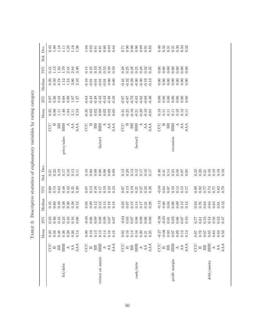
Table3:
Des
crip
tive
stat
isti
csof
exp
lan
ator
yva
riab
les
by
rati
ng
cate
gory
Mea
n25%
Med
ian
75%
Std
.D
ev.
Mea
n25%
Med
ian
75%
Std
.D
ev.
ltd/deb
t
CC
C0.4
30.2
30.4
50.6
00.2
1
pri
ce/sa
les
CC
C0.3
50.0
70.2
00.4
10.4
3B
0.5
60.4
00.6
00.7
40.2
2B
0.8
60.2
60.5
01.1
31.0
0B
B0.4
80.3
50.4
90.6
20.1
9B
B1.1
10.4
30.7
81.3
21.1
8B
BB
0.3
60.2
30.3
80.4
80.1
7B
BB
1.4
00.6
81.1
21.7
91.1
1A
0.2
90.1
60.3
00.4
20.1
6A
1.8
40.9
81.5
42.4
11.2
5A
A0.2
60.1
60.2
80.3
50.1
3A
A2.1
11.0
72.0
62.8
41.1
8A
AA
0.1
40.0
60.1
20.2
00.1
1A
AA
2.5
31.2
72.4
33.3
01.3
6
retu
rnon
ass
ets
CC
C0.0
0-0
.05
0.0
30.0
70.1
0
fact
or1
CC
C-0
.35
-0.6
3-0
.10
0.1
51.0
4B
0.1
00.0
60.0
90.1
30.0
8B
-0.0
2-0
.43
-0.0
10.4
50.8
2B
B0.1
30.0
90.1
20.1
60.0
9B
B0.0
2-0
.38
-0.0
10.5
30.8
1B
BB
0.1
30.0
80.1
20.1
70.0
8B
BB
0.0
0-0
.43
-0.0
10.5
30.8
1A
0.1
40.0
90.1
40.1
90.0
8A
0.0
2-0
.43
-0.0
10.5
30.8
0A
A0.1
60.0
70.1
80.2
30.0
9A
A0.0
2-0
.38
0.0
00.5
90.8
3A
AA
0.1
60.0
70.1
80.2
30.0
9A
AA
0.0
5-0
.29
0.0
00.5
90.8
4
cash
/deb
t
CC
C0.0
2-0
.04
0.0
30.0
70.1
3
fact
or2
CC
C-0
.31
-0.8
7-0
.45
0.2
80.7
1B
0.1
00.0
30.0
70.1
30.2
0B
-0.2
5-0
.87
-0.3
20.2
50.9
0B
B0.1
40.0
70.1
20.1
90.1
3B
B-0
.18
-0.7
9-0
.29
0.2
80.9
0B
BB
0.1
60.0
80.1
40.2
10.1
2B
BB
-0.2
1-0
.82
-0.3
00.2
50.9
0A
0.2
00.0
90.1
70.2
70.1
7A
-0.2
0-0
.82
-0.3
00.2
80.8
9A
A0.2
10.0
60.2
10.3
20.1
6A
A-0
.10
-0.6
8-0
.19
0.3
20.9
1A
AA
0.2
50.0
80.2
80.3
80.1
7A
AA
-0.0
1-0
.49
-0.1
30.3
50.8
5
pro
fit
marg
in
CC
C-0
.27
-0.3
8-0
.12
-0.0
40.4
6
rece
ssio
n
CC
C0.1
90.0
00.0
00.0
00.4
0B
-0.0
6-0
.05
0.0
00.0
40.4
1B
0.1
10.0
00.0
00.0
00.3
2B
B0.0
30.0
10.0
40.0
70.1
4B
B0.1
10.0
00.0
00.0
00.3
1B
BB
0.0
70.0
30.0
60.1
00.2
4B
BB
0.1
10.0
00.0
00.0
00.3
1A
0.0
90.0
60.0
90.1
40.5
8A
0.1
00.0
00.0
00.0
00.3
0A
A0.1
20.0
70.1
20.1
50.0
7A
A0.1
20.0
00.0
00.0
00.3
3A
AA
0.1
30.1
00.1
20.1
70.0
5A
AA
0.1
10.0
00.0
00.0
00.3
2
deb
t/ass
ets
CC
C0.8
70.7
70.8
30.9
90.2
2B
0.7
80.6
10.7
60.9
20.2
8B
B0.6
70.5
50.6
40.7
70.2
1B
BB
0.6
50.5
40.6
40.7
40.1
6A
0.6
40.5
00.6
30.7
70.1
9A
A0.6
40.5
20.6
10.8
20.1
9A
AA
0.5
90.4
70.5
20.7
90.1
6
50

Table 4: Frequency of ratings (2002Q1-2015Q3)
2002Q1-2015Q3 Surviving Firms 2002Q1-2015Q3 All Firms
Rating # of Obs Percentage Rating # of Obs PercentageD (—) (—) D 389 0.4%
CCC 41 0.6% CCC 1863 1.8%B 613 8.5% B 18190 17.3%
BB 1473 20.3% BB 25355 24.1%BBB 2963 40.8% BBB 31201 29.7%
A 1796 24.8% A 21996 20.9%AA 292 4.0% AA 5059 4.8%
AAA 77 1.1% AAA 1144 1.1%
N T NT N Avg Ti NT516 55 28380 1406 38 53999
51

Table 5: Estimation Results: Static vs AR-Probit
6-month Cum.Effect Long-run EffectStatic AR-Probit β(1 + ρ) β/(1− ρ)
ρ — 0.62debt/assets -0.77 -0.37 -0.60 -0.98
ltd/debt -3.04 -1.62 -2.63 -4.30return on assets 3.70 2.57 4.17 6.82
cash/debt -0.57 -0.53 -0.86 -1.41profit margin 0.40 0.21 0.34 0.56
price/sales 0.15 0.11 0.18 0.29factor1 -0.03 -0.04factor2 0.04 0.08
recession -0.11 -0.27const 4.56 1.75τ2 1.64 1.20τ3 2.64 2.33τ4 3.94 3.57τ5 5.26 4.78τ6 6.06 5.83
% of correct prediction 47% 44%
CCC 2% 7%B 12% 30%
BB 32% 41%BBB 78% 56%
A 29% 39%AA 0% 7%
AAA 0% 3%
Average of correct prediction 22% 26%
52

Table 6: Actual vs Predicted Ratings
AR-Probit
CCC B BB BBB A AA AAA CorPred (44%)
CCC 10 53 65 18 0 0 0 7%B 84 719 993 480 87 16 1 30%
BB 37 455 2342 2293 576 59 15 41%BBB 9 230 1950 6495 2607 289 32 56%
A 4 64 476 3196 2773 444 77 39%AA 0 6 67 254 729 74 2 7%
AAA 0 0 10 43 114 122 10 3%Avg = 26%
Static Probit
CCC B BB BBB A AA AAA CorPred (47%)
CCC 3 14 82 47 0 0 0 2%B 2 286 1269 747 73 3 0 12%
BB 0 102 1860 3485 320 10 0 32%BBB 1 11 871 9039 1671 15 4 78%
A 4 1 101 4808 2061 57 2 29%AA 0 0 13 556 560 3 0 0%
AAA 0 0 0 52 238 9 0 0%Avg = 22%
53

Table 7: Rating Transition Matrix (entire sample)
Data
CCC B BB BBB A AA AAACCC 121 22 0 0 0 0 0
B 19 2244 68 0 0 0 0BB 4 80 5510 84 0 0 0
BBB 0 2 95 11233 63 0 0A 0 0 0 106 6789 12 0
AA 0 0 0 0 31 1084 0AAA 0 0 0 0 0 8 289
AR-Probit
CCC B BB BBB A AA AAACCC 122 21 0 0 0 0 0
B 20 1088 390 0 0 0 0BB 0 101 5021 671 1 0 0
BBB 0 1 298 11752 482 0 0A 1 0 1 350 6308 104 0
AA 0 0 0 0 95 873 27AAA 0 0 0 0 0 27 110
Static Probit
CCC B BB BBB A AA AAACCC 5 3 1 0 0 0 0
B 3 340 59 3 0 0 0BB 0 64 3712 341 0 0 0
BBB 2 1 326 17677 382 0 0A 0 1 1 386 4433 21 0
AA 0 0 0 0 27 69 1AAA 0 0 0 0 0 3 3
54

Table 8: 3-Year Forecast (2012Q3-2015Q3) – Rating Transition Matrix
Data
CCC B BB BBB A AA AAACCC 23 3 0 0 0 0 0
B 3 537 12 0 0 0 0BB 0 8 1058 11 0 0 0
BBB 0 0 10 2394 20 0 0A 0 0 0 10 1390 2 0
AA 0 0 0 0 0 167 0AAA 0 0 0 0 0 1 27
AR-Probit
CCC B BB BBB A AA AAACCC 12 2 0 0 0 0 0
B 1 333 255 0 0 0 0BB 0 12 1476 405 0 0 0
BBB 0 0 29 2128 152 0 0A 0 0 0 23 802 9 0
AA 0 0 0 0 0 37 0AAA 0 0 0 0 0 0 0
Static Probit
CCC B BB BBB A AA AAACCC 0 0 0 0 0 0 0
B 1 89 9 0 0 0 0BB 0 14 728 59 0 0 0
BBB 0 0 77 3745 71 0 0A 0 0 0 78 805 0 0
AA 0 0 0 0 0 0 0AAA 0 0 0 0 0 0 0
55

Table 9: Time-varying Persistence Parameter
AR-Probit (ρt)
ρ2003 0.686ρ2004 0.711ρ2005 0.673ρ2006 0.664ρ2007 0.661ρ2008 0.762ρ2009 0.691ρ2010 0.683ρ2011 0.656ρ2012 0.635ρ2013 0.655ρ2014 0.645ρ2015 0.598
debt/assets -0.347ltd/debt -1.602
return on assets 2.681cash/debt -0.676
profit margin 0.202price/sales 0.097
factor1 -0.077factor2 -0.010
recession -0.400const 1.710τ2 1.432τ3 2.744τ4 4.136τ5 5.624τ6 6.750
% of correct prediction 44%
CCC 8%B 29%
BB 40%BBB 58%
A 39%AA 6%
AAA 6%
Average correct prediction 26%
N × T 28380
56

Table 10: Estimation Results for AR-Probit and AR-Probit with Random Effects
Balanced Panel Unbalanced Panel
AR-Probit AR-Probit RE AR-Probit AR-Probit REρ 0.623 0.500 0.782 0.484
debt/assets -0.368 -0.950 -0.282 -0.412ltd/debt -1.622 -0.160 -1.122 -0.143
return on assets 2.571 1.921 2.169 1.757cash/debt -0.535 0.304 -0.256 2.770
profit margin 0.207 0.016 0.000 0.030price/sales 0.113 0.017 0.002 0.097
d/a — 0.071 — -0.036
ltd/d — -2.711 — -2.171roa — 1.858 — 1.042
c/d — -1.771 — 0.049npm — 2.074 — -0.254
p/s — 0.119 — -0.118factor1 -0.035 -0.049 -0.141 0.089factor2 0.080 -0.011 0.161 0.333
recession -0.266 -0.275 -0.661 -0.727const 1.753 3.472 1.524 4.564
σε — 0.587 — 0.565τ2 1.200 1.775 0.578 2.352τ3 2.325 3.312 2.082 2.910τ4 3.574 5.288 3.430 3.827τ5 4.784 7.228 4.893 5.416τ6 5.831 9.326 6.373 7.397τ7 — — 7.477 8.450
57

Table 11: Dodd-Frank Threshold in Persistence Parameter ρ
AR-Probit
ρpre-DF 0.673ρpost-DF 0.635
debt/assets -0.388ltd/debt -1.542
return on assets 2.346cash/debt -0.492
profit margin 0.190price/sales 0.087
factor1 -0.104factor2 0.035
recession -0.349const 1.741τ2 1.311τ3 2.517τ4 3.872τ5 5.183τ6 6.209
% of correct prediction 44%
CCC 7%B 30%
BB 41%BBB 59%
A 35%AA 5%
AAA 3%
Average correct prediction 26%
58

A Technical Appendix
Let’s re-write the likelihood and the associated probabilities.
Lc(θ|y, x) =1
N
N∑i=1
`i(θ|yi,xi),
`i(θ|yi,xi) =
T−J∑t=1
J∑j=1
log f(yit, yi,t+j |xi; θ)
log f(yit, yi,t+j |xi; θ) = 100 logP00 + · · ·111 logP11
P00 ≡ P (yit = 0, yi,t+j = 0|xi; θ) = Φ2 (mi,t(θ),mi,t+j(θ)|r(θ))
P10 ≡ P (yit = 1, yi,t+j = 0|xi; θ) = Φ(mi,t+j(θ))− P00
P01 ≡ P (yit = 0, yi,t+j = 1|xi; θ) = Φ(mi,t(θ))− P00
P11 ≡ P (yit = 1, yi,t+j = 1|xi; θ) = 1−Φ(mi,t(θ))−Φ(mi,t+j(θ)) + P00
A.1 The Consistency Proof
Lemma 1. IE [supθ∈Θ|log f(yit, yi,t+j |xi; θ)|] <∞
Proof of Lemma 1. First, I find an upper bound for |log f(yit, yi,t+j |xi; θ)| in terms of bivariate
probabilities. Next, I will show that each of the log bivariate probabilities are bounded by the
same term. To keep the notation short, I will suppress the parameters and the data dependencies
in the probabilities whenever explicit dependency is not needed. For example, Pkl will denote
P (yit = k, yi,t+j = l | xi; θ) for {k, l} ∈ {0, 1}. Similarly, 1kl denotes 1(yit = k, yi,t+j = l).
∣∣log f(yit, yi,t+j |xi; θ)∣∣ =
∣∣100 logP00 + 110 logP10 + 101 logP01 + 111 logP11
∣∣≤∣∣logP00
∣∣+ · · ·+∣∣logP11
∣∣Let’s begin analyzing the probability logP00 by using the mean value expansion. For a θ between
θ and 0,
∣∣logP00(θ)∣∣ =
∣∣∣logP00(0) + θ′∂ logP00(θ)
∂θ
∣∣∣ =
∣∣∣∣∣log Φ2(0, 0|0) + θ′∂P00(θ)∂θ
P00(θ)
∣∣∣∣∣ ≤ 1
4+ ‖θ‖
∥∥∥∥∥∂P00(θ)∂θ
P00(θ)
∥∥∥∥∥Let’s focus on the last norm. Using the equation (28) in the section B, which provides the first
59

derivative of P00, yields
∥∥∥∥∥ ∂∂θP00
P00
∥∥∥∥∥ =
∥∥∥∥∥ ∂∂θΦ2 (mi,t,mi,t+j |r)Φ2 (mi,t,mi,t+j |r)
∥∥∥∥∥ ≤ ‖m′i,t‖∣∣∣∣∣φ(mi,t)Φ
(−rmi,t+mi,t+j√
1−r2
)Φ2 (mi,t,mi,t+j |r)
∣∣∣∣∣+ ‖m′i,t+j‖
∣∣∣∣∣φ(mi,t+j)Φ(mi,t−rmi,t+j√
1−r2
)Φ2 (mi,t,mi,t+j |r)
∣∣∣∣∣+‖r′‖√1− r2
∣∣∣∣∣φ(mi,t)φ(−rmi,t+mi,t+j√
1−r2
)Φ2 (mi,t,mi,t+j |r)
∣∣∣∣∣ (21)
We need to find upperbounds for the terms in the absolute value. The idea of these upperbounds
can be understood when one considers the special case of no autocorrelation, i.e., when ρ = 0.
Hence, if r = ρj = 0, then the ratios in (21) become
φ (mi,t) Φ(mi,t+j)
Φ(mi,t)Φ(mi,t+j)≤ c(1 + |mi,t|) and
φ (mi,t)φ(mi,t+j)
Φ(mi,t)Φ(mi,t+j)≤ c(1 + max{m2
i,t,m2i,t+j})
A non-zero autocorrelation does not change the limiting behavior of these ratios. The details are
given in the subsection B.2, in particular in the equations (39) and (41).∥∥∥∥∥ ∂∂θP00
P00
∥∥∥∥∥ ≤ c‖m′i,t‖ (1 + max{|mi,t|, |mi,t+j |})
+ c‖m′i,t+j‖ (1 + max{|mi,t|, |mi,t+j |})
+ c‖r′‖√1− r2
(1 + max{m2
i,t,m2i,t+j}
)The same upperbounds are found for other probabilities. For instance, consider the first ratio in
‖P′10/P10‖ when r = 0.
φ(mi,t)Φ(−rmi,t+mi,t+j√
1−r2
)Φ(mi,t+j)−Φ2 (mi,t,mi,t+j |r)
(r=0)=
φ(mi,t)Φ(mi,t+j)
Φ(mi,t+j)−Φ(mi,t)Φ(mi,t+j)=φ(−mi,t)
Φ(−mi,t)≤ c(1 + |mi,t|)
Thus, the limiting behavior of the ratios involving normal pdf and cdf’s is common for each proba-
bility. Therefore, if we combine all four bivariate probabilities and the associated upperbpunds, we
obtain an upper bound for the log likelihood in terms of m and its derivative m′. Without loss of
generality, let’s assume that |mi,t+j | ≤ |mi,t| and ‖m′i,t+j‖ ≤ ‖m′i,t‖.
∣∣log f(yit, yi,t+j |xi; θ)∣∣ ≤ ∣∣logP00
∣∣+ · · ·+∣∣logP11
∣∣ ≤ 1 + ‖θ‖
(∥∥∥∥∥ ∂∂θP00(θ)
P00(θ)
∥∥∥∥∥+ · · ·
∥∥∥∥∥ ∂∂θP11(θ)
P11(θ)
∥∥∥∥∥)
≤ 1 + c‖θ‖(‖m′i,t‖(1 + |mi,t|) +
‖r′‖√1− r2
(1 +m2
i,t
))60

IE
[supθ∈Θ
∣∣log f(yit, yi,t+j |xi; θ)∣∣]
≤ IE
[supθ∈Θ
∣∣logP00(θ)∣∣+ · · ·+
∣∣logP11(θ)∣∣]
≤ 1 + IE
[supθ∈Θ
c‖θ‖
(‖m′i,t(θ)‖(1 + |mi,t(θ)|) +
‖r′(θ)‖√1− r2(θ)
(1 +m2
i,t(θ)))]
≤ 1 + CIE
(supθ∈Θ‖m′i,t(θ)‖ (1 + |mi,t(θ)|)
)+ CIE
(supθ∈Θ
m2i,t(θ)
)≤ C
{IE
[supθ∈Θ
(t∑
k=0
(ρ2
1− ρ2+ k
)|ρ|k−1‖β‖‖xi,t−k‖+
t∑k=0
|ρ|k‖xi,t−k‖
)(1 +
t∑k=0
|ρ|k‖β‖‖xi,t−k‖
)]
+IE
[supθ∈Θ
t∑k=0
t∑l=0
|ρ|k+l‖β‖2‖xi,t−k‖‖xi,t−l‖
]}
≤ C
{IE
[(t∑
k=0
(1 + k)ρk‖xi,t−k‖
)(1 +
t∑k=0
ρk‖xi,t−k‖
)]+ IE
[t∑
k=0
t∑l=0
ρk+l‖xi,t−k‖‖xi,t−l‖
]}
≤ C
{t∑
k=0
(1 + k)ρkIE‖xi,t−k‖+t∑
k=0
t∑l=0
(1 + k)ρ(k+l−1)IE‖xi,t−k‖‖xi,t−l‖
},
where 1 > ρ is an upperbound for ρ. The details for each upperbound regarding |mi,t|, ‖m′i,t‖ and
m2it can be found in B.3. Thus, it follows that IE [supθ∈Θ | log f(yit, yi,t+j |xi; θ)|] <∞ provided that
IE(xixi′) is nonsingular, which implies IE‖xi‖2 <∞.
Lemma 2. θ 6= θ0 implies f(yit, yi,t+j |xi; θ) 6= f(yit, yi,t+j |xi; θ0).
Proof of Lemma 2. I already showed that IE[log f(yit, yi,t+j |xi; θ0)] ≥ IE[log f(yit, yi,t+j |xi; θ)] for all
θ ∈ Θ. This lemma shows that θ0 is the unique maximizer. It is easier to work with univariate case
as opposed to bivariate probabilities. Remember that
P(yit = 0|xi; θ) = Φ
(−√
1− ρ2
t∑k=0
ρkβ′xi,t−k
)= Φ
(t∑
k=0
ρkβ′xi,t−k
),
where β = −√
1− ρ2β. This transformation is one-to-one. Thus, identifying (ρ, β) would be the
same as identifying (ρ, β). Let’s denote xi,0:t = (x′i0, . . . , x′it)′ and rt(θ) = (ρtβ′, . . . , ρβ′, β′)′, which
are both ((t+ 1)K × 1) dimensional vectors. Note that B′t(θ)xi,0:t =∑t
k=0 ρkβ′xi,t−k.
61

θ 6= θo =⇒ Bt(θ) 6= Bt(θ0)
=⇒ B′t(θ)xi,0:t 6= B′t(θ0)xi,0:t with positive probability if IE[xi,0:tx′i,0:t] > 0
=⇒ Φ(B′t(θ)xi,0:t
)6= Φ
(B′t(θ0)xi,0:t
)with positive probability
=⇒ P(yit = 0|xi; θ) 6= P(yit = 0|xi; θ0) with positive probability
=⇒ f(yit, yi,t+j |xi; θ) 6= f(yit, yi,t+j |xi; θ0) with positive probability
We need the positive definiteness of E[xi,0:tx′i,0:t] for each t. Hence, the required condition for iden-
tification is IE[xixi′] > 0. If the parameters are identified in the univariate model, then they will also
be identified in the bivariate model since using more information will only help the identification
in estimation.
An alternative way for identification in the bivariate case would be using an approach that
is commonly used in average derivative estimation techniques (see, for instance, Stoker [1986]).
Assume that there is at least one continuous regressor, and let the first regressor, denoted by x(1)it ,
be one of the continuous regressors.
∂IE [1 (yit = 0, yi,t+j = 0) |xi; θ]
∂x(1)it
=
∂Φ2
(∑tk=0 ρ
kβ′xi,t−k,∑t+j
k=0 ρkβ′xi,t+j−k
∣∣∣∣ r = ρj)
∂x(1)it
= β1Φ
(−rmi,t +mi,t+j√
1− r2
)+ ρjβ1Φ
(mi,t − rmi,t+j√
1− r2
)Similarly,
∂IE [1 (yit = 0, yi,t+j = 0) |xi; θ]
∂x(1)i,t−1
= ρβ1Φ
(−rmi,t +mi,t+j√
1− r2
)+ ρj+1β1Φ
(mt − rmt+j√
1− r2
)= ρ
[β1Φ
(−rmi,t +mi,t+j√
1− r2
)+ ρjβ1Φ
(mi,t − rmi,t+j√
1− r2
)]= ρ
∂IE [1 (yit = 0, yi,t+j = 0) |xi; θ]
∂x(1)it
Thus, taking their ratio would isolate ρ. After identifying ρ, we can proceed to identify β in a
62

similar way as in the univarite case.
β 6= βo
=⇒ Bt(ρ, β) 6= Bt(ρ, β0) for all t
=⇒ B′t(ρ, β)xi,0:t 6= B′t(ρ, β0)xi,0:t for all t with positive probability if IE[xi,0:tx′i,0:t] > 0
=⇒ Φ2
(B′t(ρ, β)xi,0:t, B
′t+j(ρ, β)xi,0:t+j |ρj
)6= Φ2
(B′t(ρ, β0)xi,0:t, B
′t+j(ρ, β0)xi,0:t+j |ρj
)with pos. prob.
=⇒ P(yit = 0|xi; ρ, β) 6= P(yit = 0|xi; ρ, β0) with positive probability
=⇒ f(yit, yi,t+j |xi; ρ, β) 6= f(yit, yi,t+j |xi; ρ, β0) with positive probability
The third step needs some explanation since for constants (a, b, a, b) such that a > a and b < b
one can still have Φ2(a, b|r) = Φ2(a, b|r). But, this is not the case with probability one as long
as xit is a well-behaving random variable with a full support. Consider a simple case where
β 6= βo but Φ2(β′xio, β′xi1 + ρβ′xio|ρ) = Φ2(β′oxio, β
′oxi1 + ρβ′oxio|ρ). The equality holds if
β′xio > β′oxio and β′xi1 + ρβ′xio < β′oxi1 + ρβ′oxio (note that the inequalities between argu-
ments can flip without loss of generality.) Moreover, for given β, βo, and xio; xi1 is determined
uniquely since Φ2 is strictly increasing in its both arguments. Hence, any other xi1 that can
be picked with a positive probability will render β = βo, thus, will provide the identification.
The assumption IE[xixi′] > 0 ensures that we can pick another xi1 with a positive probability.
Since IE[log f(yit, yi,t+j |xi; θ0)] ≥ IE[log f(yit, yi,t+j |xi; θ)] is already shown, we can conclude that
IE[log f(yit, yi,t+j |xi; θ0)] > IE[log f(yit, yi,t+j |xi; θ)] for all θ ∈ Θ. Hence, IE[`i(θ0)] > IE[`i(θ)] for all
θ ∈ Θ.
Lemma 1 and Lemma 2 constitute the consistency proof for θ.
A.2 The Asymptotic Normality Proof
In this section, I analyze the asymptotic distribution of θ. In particular, I will prove that
√N(θ − θ0) −→d N
(0, H(θ0)−1G(θ0)H(θ0)−1
),
where
H(θ) = IE
[∂2`i(θ)
∂θ∂θ′
]= IE
T−J∑t=1
J∑j=1
∂2 log f(yit, yi,t+j |xi; θ)
∂θ∂θ′
G(θ) = IE
[∂`i(θ)
∂θ
∂`i(θ)
∂θ′
]= IE
T−J∑t=1
J∑j=1
∂ log f(yit, yi,t+j |xi; θ)
∂θ
T−J∑t=1
J∑j=1
∂ log f(yit, yi,t+j |xi; θ)
∂θ
′63
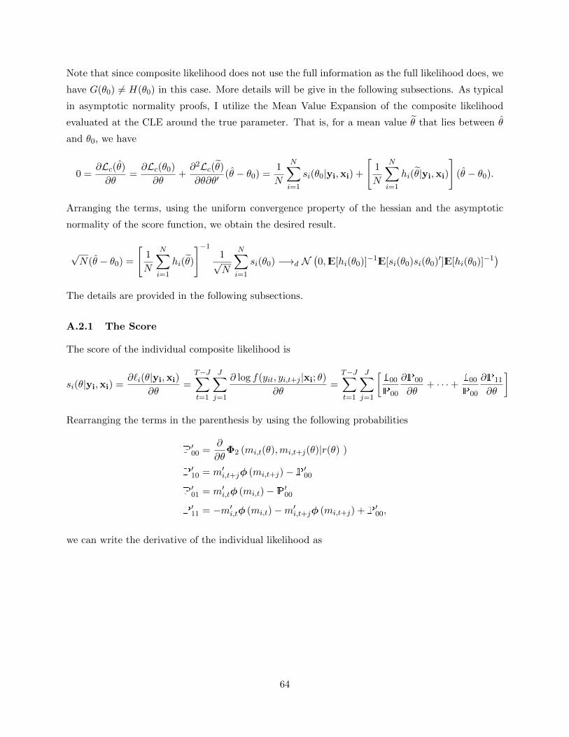
Note that since composite likelihood does not use the full information as the full likelihood does, we
have G(θ0) 6= H(θ0) in this case. More details will be give in the following subsections. As typical
in asymptotic normality proofs, I utilize the Mean Value Expansion of the composite likelihood
evaluated at the CLE around the true parameter. That is, for a mean value θ that lies between θ
and θ0, we have
0 =∂Lc(θ)∂θ
=∂Lc(θ0)
∂θ+∂2Lc(θ)∂θ∂θ′
(θ − θ0) =1
N
N∑i=1
si(θ0|yi,xi) +
[1
N
N∑i=1
hi(θ|yi,xi)
](θ − θ0).
Arranging the terms, using the uniform convergence property of the hessian and the asymptotic
normality of the score function, we obtain the desired result.
√N(θ − θ0) =
[1
N
N∑i=1
hi(θ)
]−11√N
N∑i=1
si(θ0) −→d N(0, IE[hi(θ0)]−1IE[si(θ0)si(θ0)′]IE[hi(θ0)]−1
)The details are provided in the following subsections.
A.2.1 The Score
The score of the individual composite likelihood is
si(θ|yi,xi) =∂`i(θ|yi,xi)
∂θ=
T−J∑t=1
J∑j=1
∂ log f(yit, yi,t+j |xi; θ)
∂θ=
T−J∑t=1
J∑j=1
[100
P00
∂P00
∂θ+ · · ·+ 100
P00
∂P11
∂θ
]
Rearranging the terms in the parenthesis by using the following probabilities
P′00 =
∂
∂θΦ2 (mi,t(θ),mi,t+j(θ)|r(θ) )
P′10 = m′i,t+jφ (mi,t+j)−P′00
P′01 = m′i,tφ (mi,t)−P′00
P′11 = −m′i,tφ (mi,t)−m′i,t+jφ (mi,t+j) +P′00,
we can write the derivative of the individual likelihood as
64
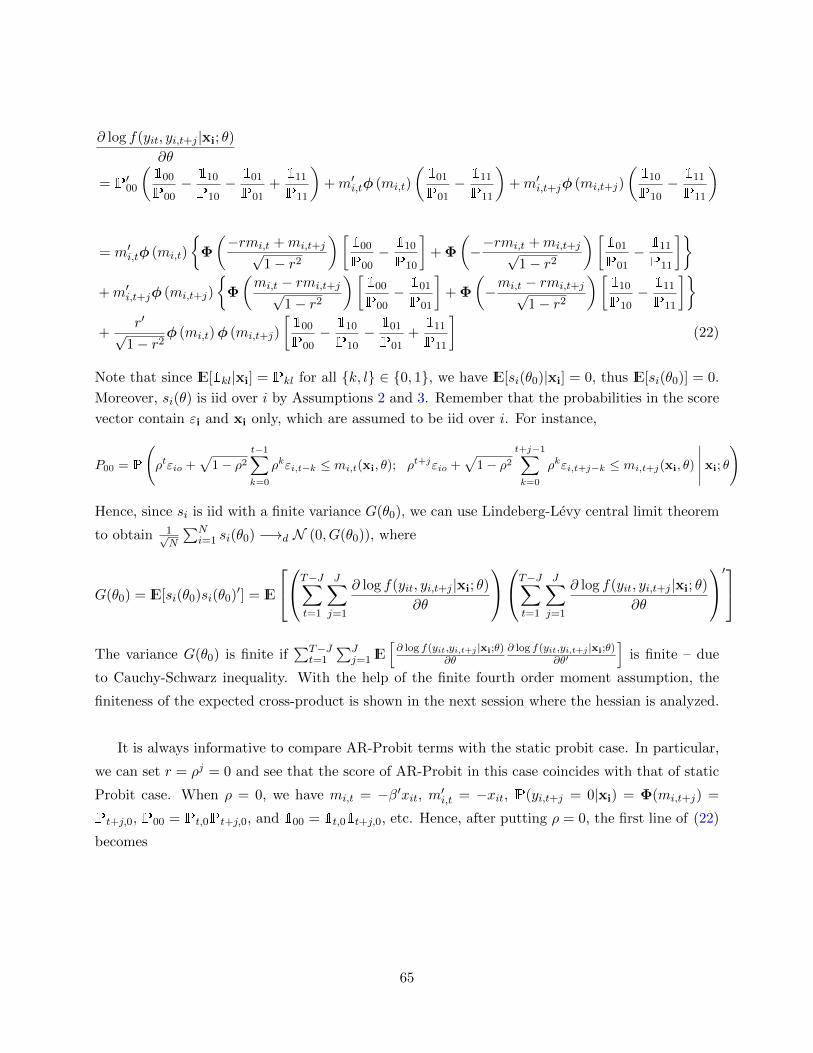
∂ log f(yit, yi,t+j |xi; θ)
∂θ
= P′00
(100
P00− 110
P10− 101
P01+111
P11
)+m′i,tφ (mi,t)
(101
P01− 111
P11
)+m′i,t+jφ (mi,t+j)
(110
P10− 111
P11
)
= m′i,tφ (mi,t)
{Φ
(−rmi,t +mi,t+j√
1− r2
)[100
P00− 110
P10
]+ Φ
(−−rmi,t +mi,t+j√
1− r2
)[101
P01− 111
P11
]}+m′i,t+jφ (mi,t+j)
{Φ
(mi,t − rmi,t+j√
1− r2
)[100
P00− 101
P01
]+ Φ
(−mi,t − rmi,t+j√
1− r2
)[110
P10− 111
P11
]}+
r′√1− r2
φ (mi,t)φ (mi,t+j)
[100
P00− 110
P10− 101
P01+111
P11
](22)
Note that since IE[1kl|xi] = Pkl for all {k, l} ∈ {0, 1}, we have IE[si(θ0)|xi] = 0, thus IE[si(θ0)] = 0.
Moreover, si(θ) is iid over i by Assumptions 2 and 3. Remember that the probabilities in the score
vector contain εi and xi only, which are assumed to be iid over i. For instance,
P00 = P
(ρtεio +
√1− ρ2
t−1∑k=0
ρkεi,t−k ≤ mi,t(xi, θ); ρt+jεio +√
1− ρ2t+j−1∑k=0
ρkεi,t+j−k ≤ mi,t+j(xi, θ)
∣∣∣∣∣ xi; θ
)
Hence, since si is iid with a finite variance G(θ0), we can use Lindeberg-Levy central limit theorem
to obtain 1√N
∑Ni=1 si(θ0) −→d N (0, G(θ0)), where
G(θ0) = IE[si(θ0)si(θ0)′] = IE
T−J∑t=1
J∑j=1
∂ log f(yit, yi,t+j |xi; θ)
∂θ
T−J∑t=1
J∑j=1
∂ log f(yit, yi,t+j |xi; θ)
∂θ
′The variance G(θ0) is finite if
∑T−Jt=1
∑Jj=1 IE
[∂ log f(yit,yi,t+j |xi;θ)
∂θ∂ log f(yit,yi,t+j |xi;θ)
∂θ′
]is finite – due
to Cauchy-Schwarz inequality. With the help of the finite fourth order moment assumption, the
finiteness of the expected cross-product is shown in the next session where the hessian is analyzed.
It is always informative to compare AR-Probit terms with the static probit case. In particular,
we can set r = ρj = 0 and see that the score of AR-Probit in this case coincides with that of static
Probit case. When ρ = 0, we have mi,t = −β′xit, m′i,t = −xit, P(yi,t+j = 0|xi) = Φ(mi,t+j) =
Pt+j,0, P00 = Pt,0Pt+j,0, and 100 = 1t,01t+j,0, etc. Hence, after putting ρ = 0, the first line of (22)
becomes
65

− xitφ(β′xit)
{Pt+j,0
[1t,01t+j,0
Pt,0Pt+j,0− 1t,11t+j,0
Pt,1Pt+j,0
]+ Pt+j,1
[1t,01t+j,1
Pt,0Pt+j,1− 1t,11t+j,1
Pt,1Pt+j,1
]}= −xitφ(β′xit)
[1t,0
Pt,0− 1t,1Pt,1
]= −xitφ(β′xit)
[1− yitPt,0
− yitPt,1
]= xitφ(β′xit)
yit −Φ(β′xit)
Φ(β′xit)Φ(−β′xit)
which is exactly the score function of the Static Probit model.
A.2.2 The Hessian
In this subsection, I compute the hessian of the composite likelihood function and show that it is
uniformly bounded. The hessian is found to be
h(θ|yi,xi) =∂2`i(θ|yi,xi)
∂θ∂θ′=
T−J∑t=1
J∑j=1
∂2 log f(yit, yi,t+j |xi; θ)
∂θ∂θ′
where
∂2 log f(yit, yi,t+j |xi; θ)
∂θ∂θ′=100
P00
(∂2P00
∂θ∂θ′− 1
P00
∂P00
∂θ
∂P00
∂θ′
)+ · · ·+ 111
P11
(∂2P11
∂θ∂θ′− 1
P11
∂P11
∂θ
∂P11
∂θ′
)An upperbound for the individual hessian h(θ|yi,xi) will depend on an upperbound for the second
derivative of log-likelihood.
∥∥∥∂2 log f(yit, yi,t+j |xi; θ)
∂θ∂θ′
∥∥∥ ≤ ∥∥∥ 1
P00
∂2P00
∂θ∂θ′− 1
P200
∂P00
∂θ
∂P00
∂θ′
∥∥∥+ · · ·+∥∥∥ 1
P11
∂2P11
∂θ∂θ′− 1
P211
∂P11
∂θ
∂P11
∂θ′
∥∥∥The norms are analyzed in the section B.2. For instance, the first norm – as well as other three
norms – are bounded by
∥∥∥∂2 log f(yit, yi,t+j |xi; θ)
∂θ∂θ′
∥∥∥ (23)
≤ c(1 + |mi,t|)(∥∥∥∂2mi,t
∂θ∂θ′
∥∥∥+∥∥∥∂2mi,t+j
∂θ∂θ′
∥∥∥+∥∥∥ ∂2r
∂θ∂θ′
∥∥∥) (24)
+ c(1 +m2i,t)
(∥∥∥∂mi,t
∂θ
∂mi,t
∂θ′
∥∥∥+∥∥∥∂mi,t+j
∂θ
∂mi,t+j
∂θ′
∥∥∥+∥∥∥∂mi,t
∂θ
∂mi,t+j
∂θ′
∥∥∥+∥∥∥∂mi,t+j
∂θ
∂mi,t
∂θ′
∥∥∥) (25)
+ c(1 + |mi,t|3)
(∥∥∥∂mi,t
∂θ
∂r
∂θ′
∥∥∥+∥∥∥∂r∂θ
∂mi,t
∂θ′
∥∥∥+∥∥∥∂mi,t+j
∂θ
∂r
∂θ′
∥∥∥+∥∥∥∂r∂θ
∂mi,t+j
∂θ′
∥∥∥) (26)
+ c(1 +m4i,t)∥∥∥∂r∂θ
∂r
∂θ′
∥∥∥ (27)
66

Note that, the norms in (25) contain norms of second order moments of xi; the norms in (26)
contain norms of first order moments of xi; and∥∥∥∂r∂θ ∂r∂θ′∥∥∥ in (27) is finite. Also note that, except the
line (24), every other line contains norms of the fourth order moment of xi. Thus, if IE‖xi‖4 <∞,
then
IE
[supθ∈Θ‖h(θ|yi,xi)‖
]≤
T−J∑t=1
J∑j=1
IE
[supθ∈Θ
∥∥∥∂2 log f(yit, yi,t+j |xi; θ)
∂θ∂θ′
∥∥∥] <∞This condition gives the uniform convergence of 1
N
∑Ni=1 h(θ|yi,xi) for any consistent estimator θ.
Hence,
1
N
N∑i=1
h(θ|yi,xi) −→p H(θ0)
H(θ0) = IE [h(θ0|yi,xi)] =T−J∑t=1
J∑j=1
IE
[∂2 log f(yit, yi,t+j |xi; θ0)
∂θ∂θ′
]
We need H(θ0) to be nonsingular. It is usually hard to prove negative definiteness of the hessian
matrix in non-linear models. However, with composite likelihood we can utilize its nice features
that it borrows from the full likelihood. In particular, note that even thought the Bartlett equality
does not hold for the composite likelihood, in general, it still holds for each piece of the composite
likelihood. That is, IE[∂`i(θo)∂θ∂`i(θo)∂θ′ ] 6= −IE[∂
2`i(θo)∂θ∂θ′ ]. However,
IE
[∂ log f(yit, yi,t+j |xi; θ0)
∂θ
∂ log f(yit, yi,t+j |xi; θ0)
∂θ′
]= −IE
[∂2 log f(yit, yi,t+j |xi; θ0)
∂θ∂θ′
]< 0
Hence, H(θ0) is invertible. Therefore, we can conclude that, for any consistent estimator θ,
[1
N
N∑i=1
h(θ|yi,xi)
]−1
−→p H(θ0)−1
B Mathematical Details
This section analyzes mathematical properties of functions of normal density and normal cumulative
distribution, especially the ones that are need throughout the analysis in this paper.
B.1 Derivatives of a Bivariate Normal Distribution
The derivative of bivariate normal distribution with respect to the mean and variance parameters are
analyzed in this subsection. To facilitate the algebra, I use the change of variables in the following
67
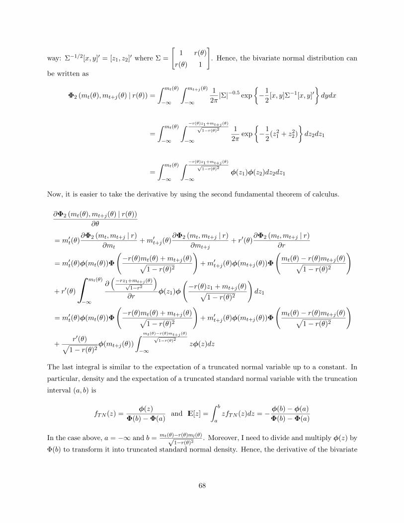
way: Σ−1/2[x, y]′ = [z1, z2]′ where Σ =
[1 r(θ)
r(θ) 1
]. Hence, the bivariate normal distribution can
be written as
Φ2 (mt(θ),mt+j(θ) | r(θ)) =
∫ mt(θ)
−∞
∫ mt+j(θ)
−∞
1
2π|Σ|−0.5 exp
{−1
2[x, y]Σ−1[x, y]′
}dydx
=
∫ mt(θ)
−∞
∫ −r(θ)z1+mt+j(θ)√1−r(θ)2
−∞
1
2πexp
{−1
2(z2
1 + z22)
}dz2dz1
=
∫ mt(θ)
−∞
∫ −r(θ)z1+mt+j(θ)√1−r(θ)2
−∞φ(z1)φ(z2)dz2dz1
Now, it is easier to take the derivative by using the second fundamental theorem of calculus.
∂Φ2 (mt(θ),mt+j(θ) | r(θ))∂θ
= m′t(θ)∂Φ2 (mt,mt+j | r)
∂mt+m′t+j(θ)
∂Φ2 (mt,mt+j | r)∂mt+j
+ r′(θ)∂Φ2 (mt,mt+j | r)
∂r
= m′t(θ)φ(mt(θ))Φ
(−r(θ)mt(θ) +mt+j(θ)√
1− r(θ)2
)+m′t+j(θ)φ(mt+j(θ))Φ
(mt(θ)− r(θ)mt+j(θ)√
1− r(θ)2
)
+ r′(θ)
∫mt(θ)
−∞
∂(−rz1+mt+j(θ)√
1−r2
)∂r
φ(z1)φ
(−r(θ)z1 +mt+j(θ)√
1− r(θ)2
)dz1
= m′t(θ)φ(mt(θ))Φ
(−r(θ)mt(θ) +mt+j(θ)√
1− r(θ)2
)+m′t+j(θ)φ(mt+j(θ))Φ
(mt(θ)− r(θ)mt+j(θ)√
1− r(θ)2
)
+r′(θ)√
1− r(θ)2φ(mt+j(θ))
∫ mt(θ)−r(θ)mt+j(θ)√1−r(θ)2
−∞zφ(z)dz
The last integral is similar to the expectation of a truncated normal variable up to a constant. In
particular, density and the expectation of a truncated standard normal variable with the truncation
interval (a, b) is
fTN (z) =φ(z)
Φ(b)−Φ(a)and IE[z] =
∫ b
azfTN (z)dz = − φ(b)− φ(a)
Φ(b)−Φ(a)
In the case above, a = −∞ and b = mt(θ)−r(θ)ml(θ)√1−r(θ)2
. Moreover, I need to divide and multiply φ(z) by
Φ(b) to transform it into truncated standard normal density. Hence, the derivative of the bivariate
68
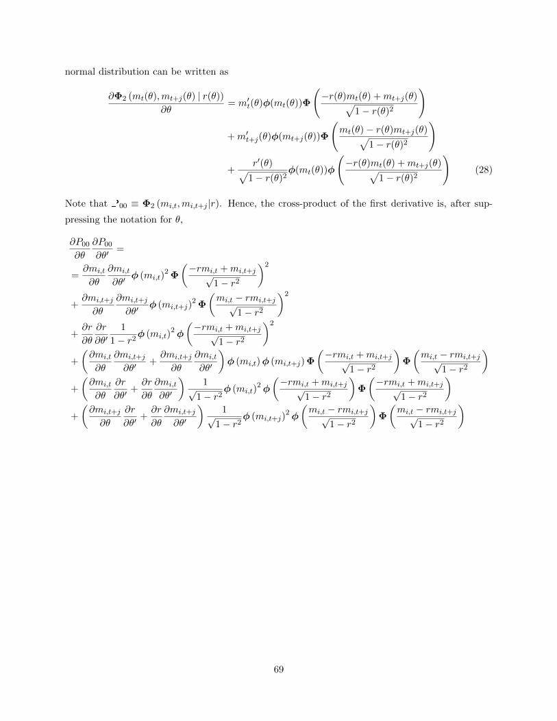
normal distribution can be written as
∂Φ2 (mt(θ),mt+j(θ) | r(θ))∂θ
= m′t(θ)φ(mt(θ))Φ
(−r(θ)mt(θ) +mt+j(θ)√
1− r(θ)2
)
+m′t+j(θ)φ(mt+j(θ))Φ
(mt(θ)− r(θ)mt+j(θ)√
1− r(θ)2
)
+r′(θ)√
1− r(θ)2φ(mt(θ))φ
(−r(θ)mt(θ) +mt+j(θ)√
1− r(θ)2
)(28)
Note that P00 ≡ Φ2 (mi,t,mi,t+j |r). Hence, the cross-product of the first derivative is, after sup-
pressing the notation for θ,
∂P00
∂θ
∂P00
∂θ′=
=∂mi,t
∂θ
∂mi,t
∂θ′φ (mi,t)
2 Φ
(−rmi,t +mi,t+j√
1− r2
)2
+∂mi,t+j
∂θ
∂mi,t+j
∂θ′φ (mi,t+j)
2 Φ
(mi,t − rmi,t+j√
1− r2
)2
+∂r
∂θ
∂r
∂θ′1
1− r2φ (mi,t)
2φ
(−rmi,t +mi,t+j√
1− r2
)2
+
(∂mi,t
∂θ
∂mi,t+j
∂θ′+∂mi,t+j
∂θ
∂mi,t
∂θ′
)φ (mi,t)φ (mi,t+j) Φ
(−rmi,t +mi,t+j√
1− r2
)Φ
(mi,t − rmi,t+j√
1− r2
)+
(∂mi,t
∂θ
∂r
∂θ′+∂r
∂θ
∂mi,t
∂θ′
)1√
1− r2φ (mi,t)
2φ
(−rmi,t +mi,t+j√
1− r2
)Φ
(−rmi,t +mi,t+j√
1− r2
)+
(∂mi,t+j
∂θ
∂r
∂θ′+∂r
∂θ
∂mi,t+j
∂θ′
)1√
1− r2φ (mi,t+j)
2φ
(mi,t − rmi,t+j√
1− r2
)Φ
(mi,t − rmi,t+j√
1− r2
)
69
The second derivative would be
∂2P00
∂θ∂θ′=∂2mi,t
∂θ∂θ′φ (mt) Φ
(−rmt +mt+j√
1− r2
)+∂mi,t
∂θ
∂mi,t
∂θ′(−mi,t)φ (mi,t) Φ
(−rmi,t +mi,t+j√
1− r2
)+∂mi,t
∂θ
∂
∂θ′
[−rmi,t +mi,t+j√
1− r2
]φ (mi,t)φ
(−rmi,t +mi,t+j√
1− r2
)+∂2mi,t+j
∂θ∂θ′φ (mi,t+j) Φ
(mi,t − rmi,t+j√
1− r2
)+∂mi,t+j
∂θ
∂mi,t+j
∂θ′(−mi,t+j)φ (mi,t+j) Φ
(mi,t − rmi,t+j√
1− r2
)+∂mi,t+j
∂θ
∂
∂θ′
[mi,t − rmi,t+j√
1− r2
]φ (mi,t+j)φ
(mi,t − rmi,t+j√
1− r2
)+
∂
∂θ′
[r′√
1− r2
]φ (mi,t)φ
(−rmi,t +mi,t+j√
1− r2
)+∂r
∂θ
∂mi,t
∂θ′1√
1− r2(−mi,t)φ (mi,t)φ
(−rmi,t +mi,t+j√
1− r2
)+∂r
∂θ
∂
∂θ′
[−rmi,t +mi,t+j√
1− r2
]1√
1− r2
(−−rmi,t +mi,t+j√
1− r2
)φ (mi,t)φ
(−rmi,t +mi,t+j√
1− r2
)The following terms will be replaced in the above equation.
∂
∂θ
[−rmi,t +mi,t+j√
1− r2
]= − r√
1− r2
∂mi,t
∂θ+
1√1− r2
∂mi,t+j
∂θ−
∂r∂θ√
1− r2
(mi,t − rmi,t+j√
1− r2
)∂
∂θ
[mi,t − rmi,t+j√
1− r2
]=
1√1− r2
∂mi,t
∂θ− r√
1− r2
∂mi,t+j
∂θ−
∂r∂θ√
1− r2
(−rmi,t +mi,t+j√
1− r2
)∂
∂θ′
[r′√
1− r2
]=
∂2r∂θ∂θ′√1− r2
+∂r∂θ
∂r∂θ′
1− r2
r√1− r2
70
Hence, the second derivative of P00 is found to be
∂2P00
∂θ∂θ′
=∂2mi,t
∂θ∂θ′φ (mi,t) Φ
(−rmi,t +mi,t+j√
1− r2
)+∂2mi,t+j
∂θ∂θ′φ (mi,t+j) Φ
(mi,t − rmi,t+j√
1− r2
)+
∂2r
∂θ∂θ′1√
1− r2φ (mi,t)φ
(−rmi,t +mi,t+j√
1− r2
)+∂mi,t
∂θ
∂mi,t
∂θ′
[−mi,tφ (mi,t) Φ
(−rmi,t +mi,t+j√
1− r2
)− r√
1− r2φ (mi,t)φ
(−rmi,t +mi,t+j√
1− r2
)]+∂mi,t+j
∂θ
∂mi,t+j
∂θ′
[−mi,t+jφ (mi,t+j) Φ
(mi,t − rmi,t+j√
1− r2
)− r√
1− r2φ (mi,t+j)φ
(mi,t − rmi,t+j√
1− r2
)]+∂r
∂θ
∂r
∂θ′1
(1− r2)3/2φ (mi,t)φ
(−rmi,t +mi,t+j√
1− r2
)[r +
mi,t − rmi,t+j√1− r2
−rmi,t +mi,t+j√1− r2
]+
(∂mi,t
∂θ
∂mi,t+j
∂θ′+∂mi,t+j
∂θ
∂mi,t
∂θ′
)1√
1− r2φ (mi,t)φ
(−rmi,t +mi,t+j√
1− r2
)+
(∂mi,t
∂θ
∂r
∂θ′+∂r
∂θ
∂mi,t
∂θ′
)1
1− r2φ (mi,t)φ
(−rmi,t +mi,t+j√
1− r2
)[−mi,t − rmi,t+j√
1− r2
]+
(∂mi,t+j
∂θ
∂r
∂θ′+∂r
∂θ
∂mi,t+j
∂θ′
)1
1− r2φ (mi,t)φ
(−rmi,t +mi,t+j√
1− r2
)[−−rmi,t +mi,t+j√
1− r2
]
71

The following will be useful in computing the hessian.
1
P00
∂2P00
∂θ∂θ′− 1
P200
∂P00
∂θ
∂P00
∂θ′(29)
=∂2mi,t
∂θ∂θ′
φ (mi,t) Φ(−rmi,t+mi,t+j√
1−r2
)Φ2 (mi,t,mi,t+j |r)
(30)
+∂2mi,t+j
∂θ∂θ′
φ (mi,t+j) Φ(mi,t−rmi,t+j√
1−r2
)Φ2 (mi,t,mi,t+j |r)
(31)
+∂2r
∂θ∂θ′1√
1− r2
φ (mi,t)φ(−rmi,t+mi,t+j√
1−r2
)Φ2 (mi,t,mi,t+j |r)
(32)
+∂mi,t
∂θ
∂mi,t
∂θ′
φ (mi,t) Φ(−rmi,t+mi,t+j√
1−r2
)Φ2 (mi,t,mi,t+j |r)
×
−mi,t −r√
1− r2
φ(−rmi,t+mi,t+j√
1−r2
)Φ(−rmi,t+mi,t+j√
1−r2
) − φ (mi,t) Φ(−rmi,t+mi,t+j√
1−r2
)Φ2 (mi,t,mi,t+j |r)
(33)
+∂mi,t+j
∂θ
∂mi,t+j
∂θ′
φ (mi,t+j) Φ(mi,t−rmi,t+j√
1−r2
)Φ2 (mi,t,mi,t+j |r)
×
−mi,t+j −r√
1− r2
φ(mi,t−rmi,t+j√
1−r2
)Φ(mi,t−rmi,t+j√
1−r2
) − φ (mi,t+j) Φ(mi,t−rmi,t+j√
1−r2
)Φ2 (mi,t,mi,t+j |r)
(34)
+∂r
∂θ
∂r
∂θ′1
(1− r2)3/2
φ (mi,t)φ(−rmi,t+mi,t+j√
1−r2
)Φ2 (mi,t,mi,t+j |r)
×
r +mi,t − rmi,t+j√
1− r2
−rmi,t +mi,t+j√1− r2
−√
1− r2φ (mi,t)φ
(−rmi,t+mi,t+j√
1−r2
)Φ2 (mi,t,mi,t+j |r)
(35)
+
(∂mi,t
∂θ
∂mi,t+j
∂θ′+∂mi,t+j
∂θ
∂mi,t
∂θ′
) φ (mi,t)φ(−rmi,t+mi,t+j√
1−r2
)Φ2 (mt,mt+j |r)
×
1√1− r2
−Φ(−rmi,t+mi,t+j√
1−r2
)φ(−rmi,t+mi,t+j√
1−r2
) φ (mi,t+j) Φ(mi,t−rmi,t+j√
1−r2
)Φ2 (mi,t,mi,t+j |r)
(36)
+
(∂mi,t
∂θ
∂r
∂θ′+∂r
∂θ
∂mi,t
∂θ′
)1
1− r2
φ (mi,t)φ(−rmi,t+mi,t+j√
1−r2
)Φ2 (mi,t,mi,t+j |r)
×
−mi,t − rmi,t+j√1− r2
−√
1− r2φ (mi,t) Φ
(−rmi,t+mi,t+j√
1−r2
)Φ2 (mi,t,mi,t+j |r)
(37)
+
(∂mi,t+j
∂θ
∂r
∂θ′+∂r
∂θ
∂mi,t+j
∂θ′
)1
1− r2
φ (mi,t)φ(−rmi,t+mi,t+j√
1−r2
)Φ2 (mi,t,mi,t+j |r)
×
−−rmi,t +mi,t+j√1− r2
−√
1− r2φ (mi,t+j) Φ
(mi,t−rmi,t+j√
1−r2
)Φ2 (mi,t,mi,t+j |r)
(38)72
The limiting behavior of∥∥∥ 1P00
∂2P00∂θ∂θ′ −
1P
200
∂P00∂θ
∂P00∂θ′
∥∥∥ will be analyzed in Section B.2
B.2 Limits on Functions of Univariate and Bivariate Normal Distribution
The ratio φ(x)/Φ(x) is known to be bounded by C(1 + |x|). Note that the ratio approaches 0 as x
approaches positive infinity, and approaches to the negative 45 degree line as x approaches negative
infinity. One can show it by taking the limit and using L’Hopital rule, i.e., limx→−∞φ(x)/Φ(x) =
limx→−∞−xφ(x)/φ(x). Hence, the ratio goes to∞ with a linear rate. A slightly more general case
will be needed for the analysis. Let a > 0 and c > 0, where it is easy to calculate for other cases
too.
limx→−∞
φ(ax+ b)
Φ(cx+ d)= lim
x→−∞
−a(ax+ b)φ(ax+ b)
cφ(cx+ d)=
0 if a > c
0 if a = c and b > d
∞ if a < c
∞ if a = c and b < d
limx→−∞−(ax+ b) if (a, b) = (c, d)
Depending on the parameters, ratio of two normal densities is also a normal density up to a constant
multiplicative term. For constants (a, b, c, d) with |a| > |c|, a straightforward calculation yields
φ(ax+ b)
φ(cx+ d)=φ(√
a2 − c2x+ ab−cd√a2−c2
)φ(
ad−bc√a2−c2
)If |a| < |c|, then we can consider the reciprocal of the ratio, which will give again a normal density.
Next, I will analyze the limiting behavior of two ratios that appear throughout the analysis.
Claim 1. The following ratio diverges to ∞ at a linear rate. In particular,
φ (mt) Φ(−rmt+mt+j√
1−r2
)Φ2 (mt,mt+j |r)
≤ c (1 + max{|mt|, |mt+j |}) (39)
I will prove the claim by looking at different cases on mt and mt+j.
Proof.
Case 1. mt: fixed, mt+j →∞The ratio in (39) is finite since
φ (mt) Φ(−rmt+mt+j√
1−r2
)Φ2 (mt,mt+j |r)
−→ φ (mt)
Φ (mt)<∞
73

Case 2. mt: fixed, mt+j → −∞The ratio in (39) converges to 0, if r > 0. Otherwise, (39) diverges to ∞ with a linear rate, that
is, (39) is bounded by a multiple of |mt+j |. We’ll use L’Hopital rule due to 0/0 indeterminacy.
∂(·)∂mt+j=⇒
1√1−r2φ (mt)φ
(−rmt+mt+j√
1−r2
)φ (mt+j) Φ
(mt−rmt+j√
1−r2
) = c1
φ(
r√1−r2 (mt+j + c2)
)Φ(mt−rmt+j√
1−r2
) {−→ 0
1 = 0 if r > 0
≤ c(1 + |mt+j |) if r < 0
(40)
Case 3. mt →∞, mt+j: fixed
The ratio in (39) converges to 0 since
φ (mt) Φ(−rmt+mt+j√
1−r2
)Φ2 (mt,mt+j |r)
−→ 0
Φ (mt+j)= 0
Case 4. mt → −∞, mt+j: fixed
The ratio in (39) is bounded by a multiple of |mt|.
∂(·)∂mt=⇒−mtφ (mt) Φ
(−rmt+mt+j√
1−r2
)− r√
1−r2φ (mt)φ(−rmt+mt+j√
1−r2
)φ (mt) Φ
(−rmt+mt+j√
1−r2
) = −mt −r√
1− r2
φ(−rmt+mt+j√
1−r2
)Φ(−rmt+mt+j√
1−r2
)
A≈ −mt +
r√1− r2
−rmt +mt+j√1− r2
=mt − rmt+j√
1− r2≤ c (1 + |mt|)
Case 5. mt →∞, mt+j →∞The ratio in (39) converges to 0.
φ (mt) Φ(−rmt+mt+j√
1−r2
)Φ2 (mt,mt+j |r)
−→ 0
1= 0
Case 6. mt →∞, mt+j = kmt with k < 0 and k < r
The ratio in (39) is bounded by a multiple of |mt|.
φ (mt) Φ(−rmt+mt+j√
1−r2
)Φ2 (mt,mt+j |r)
=φ (mt) Φ
(k−r√1−r2mt
)Φ (mt, kmt|r)
−→ 0× 0
0
74
∂(·)∂mt=⇒−mtφ (mt) Φ
(k−r√1−r2mt
)+ k−r√
1−r2φ (mt)φ(
k−r√1−r2mt
)φ (mt) Φ
(k−r√1−r2mt
)+ kφ(kmt)Φ
(1−kr√1−r2mt
) =
−mt
Φ
(k−r√1−r2
mt
)φ
(k−r√1−r2
mt
) + k−r√1−r2
Φ
(k−r√1−r2
mt
)φ
(k−r√1−r2
mt
) + kφ(kmt)Φ
(1−kr√1−r2
mt
)φ(mt)φ
(k−r√1−r2
mt
)
=
−mt
Φ
(k−r√1−r2
mt
)φ
(k−r√1−r2
mt
) + k−r√1−r2
Φ
(k−r√1−r2
mt
)φ
(k−r√1−r2
mt
) + kΦ
(1−kr√1−r2
mt
)φ
(1−kr√1−r2
mt
)A≈
−mt−√
1−r2(k−r)
1mt− k−r√
1−r2
−√
1−r2(k−r)
1mt
+k−√
1−r2(1−kr)
1mt
≤ c (1 + |mt|) if 1− kr < 0
−mt−√
1−r2(k−r)
1mt− k−r√
1−r2
−√
1−r2(k−r)
1mt
+kΦ(0)φ(0)
−→ c <∞ if 1− kr = 0
−mt−√
1−r2(k−r)
1mt− k−r√
1−r2
−√
1−r2(k−r)
1mt
+k exp
(1−kr√1−r2
mt
) −→ 0 if 1− kr > 0
Case 7. mt →∞, mt+j = kmt with k = r < 0.
The ratio in (39) is bounded by a multiple of |mt|.
φ (mt) Φ(−rmt+mt+j√
1−r2
)Φ2 (mt,mt+j |r)
=φ (mt) Φ(0)
Φ (mt, rmt|r)−→ 0
0
∂(·)∂mt=⇒ −mtφ (mt) Φ(0)
φ (mt) Φ(0) + rφ(rmt)Φ(√
1− r2mt)=
−mt
12 + rΦ(
√1−r2mt)
φ(√
1−r2mt)
A≈ −mt
12 −
r√1−r2
1mt
≤ c (1 + |mt|)
Case 8. mt →∞, mt+j = kmt with −1 < r < k < 0.
The ratio in (39) is bounded by a multiple of |mt|.
φ (mt) Φ(−rmt+mt+j√
1−r2
)Φ2 (mt,mt+j |r)
=φ (mt) Φ
(k−r√1−r2mt
)Φ (mt, kmt|r)
−→ 0× 1
0
∂(·)∂mt=⇒ −mtφ (mt)
φ (mt) Φ(
k−r√1−r2mt
)+ kφ(kmt)Φ
(1−kr√1−r2mt
) =−mt
12 + rΦ(
√1−r2mt)
φ(√
1−k2mt)
A≈ −mt
12 − r × 0
≤ c (1 + |mt|)
Note that Φ(√
1− r2mt)/φ(√
1− k2mt)→ 0 exponentially fast since√
1− r2 >√
1− k2.
Case 9. mt → −∞, mt+j = kmt with k < r
75
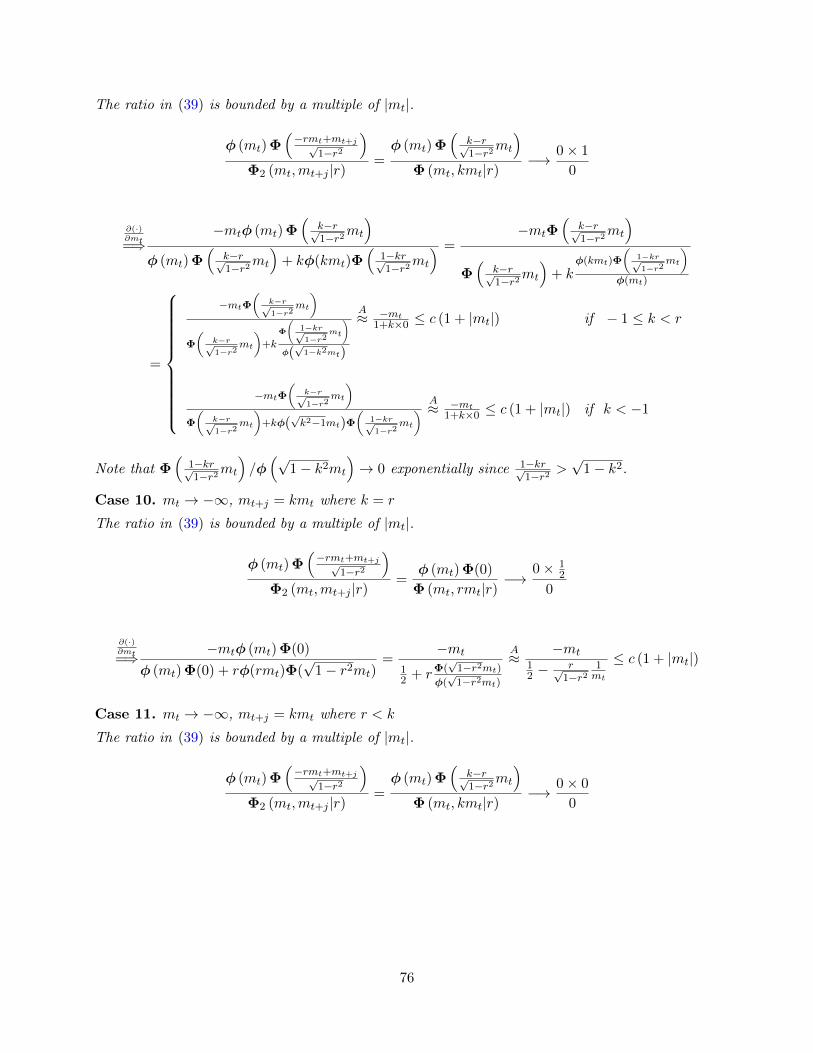
The ratio in (39) is bounded by a multiple of |mt|.
φ (mt) Φ(−rmt+mt+j√
1−r2
)Φ2 (mt,mt+j |r)
=φ (mt) Φ
(k−r√1−r2mt
)Φ (mt, kmt|r)
−→ 0× 1
0
∂(·)∂mt=⇒
−mtφ (mt) Φ(
k−r√1−r2mt
)φ (mt) Φ
(k−r√1−r2mt
)+ kφ(kmt)Φ
(1−kr√1−r2mt
) =−mtΦ
(k−r√1−r2mt
)Φ(
k−r√1−r2mt
)+ k
φ(kmt)Φ
(1−kr√1−r2
mt
)φ(mt)
=
−mtΦ(
k−r√1−r2
mt
)
Φ
(k−r√1−r2
mt
)+k
Φ
(1−kr√1−r2
mt
)φ(√
1−k2mt)
A≈ −mt
1+k×0 ≤ c (1 + |mt|) if − 1 ≤ k < r
−mtΦ(
k−r√1−r2
mt
)Φ
(k−r√1−r2
mt
)+kφ(
√k2−1mt)Φ
(1−kr√1−r2
mt
) A≈ −mt
1+k×0 ≤ c (1 + |mt|) if k < −1
Note that Φ(
1−kr√1−r2mt
)/φ(√
1− k2mt
)→ 0 exponentially since 1−kr√
1−r2 >√
1− k2.
Case 10. mt → −∞, mt+j = kmt where k = r
The ratio in (39) is bounded by a multiple of |mt|.
φ (mt) Φ(−rmt+mt+j√
1−r2
)Φ2 (mt,mt+j |r)
=φ (mt) Φ(0)
Φ (mt, rmt|r)−→
0× 12
0
∂(·)∂mt=⇒ −mtφ (mt) Φ(0)
φ (mt) Φ(0) + rφ(rmt)Φ(√
1− r2mt)=
−mt
12 + rΦ(
√1−r2mt)
φ(√
1−r2mt)
A≈ −mt
12 −
r√1−r2
1mt
≤ c (1 + |mt|)
Case 11. mt → −∞, mt+j = kmt where r < k
The ratio in (39) is bounded by a multiple of |mt|.
φ (mt) Φ(−rmt+mt+j√
1−r2
)Φ2 (mt,mt+j |r)
=φ (mt) Φ
(k−r√1−r2mt
)Φ (mt, kmt|r)
−→ 0× 0
0
76

∂(·)∂mt=⇒−mtφ (mt) Φ
(k−r√1−r2mt
)+ k−r√
1−r2φ (mt)φ(
k−r√1−r2mt
)φ (mt) Φ
(k−r√1−r2mt
)+ kφ(kmt)Φ
(1−kr√1−r2mt
) =
−mt
Φ
(k−r√1−r2
mt
)φ
(k−r√1−r2
mt
) + k−r√1−r2
Φ
(k−r√1−r2
mt
)φ
(k−r√1−r2
mt
) + kφ(kmt)Φ
(1−kr√1−r2
mt
)φ(mt)φ
(k−r√1−r2
mt
)
=
−mt
Φ
(k−r√1−r2
mt
)φ
(k−r√1−r2
mt
) + k−r√1−r2
Φ
(k−r√1−r2
mt
)φ
(k−r√1−r2
mt
) + kΦ
(1−kr√1−r2
mt
)φ
(1−kr√1−r2
mt
)A≈−mt
−√
1−r2(k−r)
1mt− k−r√
1−r2
−√
1−r2(k−r)
1mt
+ k−√
1−r2(1−kr)
1mt
≤ c (1 + |mt|)
Note thatφ(mt)φ
(k−r√1−r2
mt
)φ(kmt)
= φ(
1−kr√1−r2mt
).
Claim 2. The following ratio diverges to ∞ at a quadratic rate. In particular,
φ (mt)φ(−rmt+mt+j√
1−r2
)Φ2 (mt,mt+j |r)
≤ c(1 + max{m2
t ,m2t+j}
)(41)
I will prove the claim by looking at different cases on mt and mt+j.
Proof.
Case 1. mt: fixed, mt+j →∞The ratio in (41) is finite since
φ (mt)φ(−rmt+mt+j√
1−r2
)Φ2 (mt,mt+j |r)
−→ 0
Φ (mt)= 0
Case 2. mt: fixed, mt+j → −∞The ratio in (41) converges to 0, if r > 0. Otherwise, (41) diverges to ∞ with a quadratic rate, that
is, (41) is bounded by a multiple of |mt+j |2. We’ll use the results in (40).
∂(·)∂mt+j=⇒ − −rmt +mt+j√
1− r2
1√1−r2φ (mt)φ
(−rmt+mt+j√
1−r2
)φ (mt+j) Φ
(mt−rmt+j√
1−r2
) {−→ 0 if r > 0
≤ c(1 + |mt+j |2) if r < 0
77

Case 3. mt →∞, mt+j: fixed
The ratio in (39) converges to 0 since
φ (mt)φ(−rmt+mt+j√
1−r2
)Φ2 (mt,mt+j |r)
−→ 0
Φ (mt+j)= 0
Case 4. mt → −∞, mt+j: fixed
The ratio in (41) is bounded by a multiple of |mt|2.
φ (mt)φ(−rmt+mt+j√
1−r2
)Φ2 (mt,mt+j |r)
−→ 0
0
∂(·)∂mt=⇒−mtφ (mt)φ
(−rmt+mt+j√
1−r2
)+ r√
1−r2−rmt+mt+j√
1−r2 φ (mt)φ(−rmt+mt+j√
1−r2
)φ (mt) Φ
(−rmt+mt+j√
1−r2
)
=φ (mt)φ
(−rmt+mt+j√
1−r2
) [−mt + r√
1−r2−rmt+mt+j√
1−r2
]φ (mt) Φ
(−rmt+mt+j√
1−r2
) = −φ(−rmt+mt+j√
1−r2
)Φ(−rmt+mt+j√
1−r2
)mt − rmt+j√1− r2
A≈ − r√
1− r2
−rmt +mt+j√1− r2
mt − rmt+j√1− r2
≤ c(1 + |mt+j |2)
Case 5. mt →∞, mt+j →∞The ratio in (41) converges to 0.
φ (mt)φ(−rmt+mt+j√
1−r2
)Φ2 (mt,mt+j |r)
−→ 0
1= 0
For the following cases when mt+j = kmt, we will transform the ratio (41) into
φ (mt)φ(−rmt+mt+j√
1−r2
)Φ2 (mt,mt+j |r)
=φ (mt) Φ
(k−r√1−r2mt
)φ (mt, kmt|r)
=
φ
(√1 + (k−r)2
1−r2 mt
)φ (mt, kmt|r)
78

Moreover, the derivative of the numerator and denumerator yields
−[1 + (k−r)2
1−r2
]mtφ
(√1 + (k−r)2
1−r2 mt
)φ (mt) Φ
(k−r√1−r2mt
)+ kφ(kmt)Φ
(1−kr√1−r2mt
) =−[1 + (k−r)2
1−r2
]mt
Φ
(k−r√1−r2
mt
)φ
(k−r√1−r2
mt
) + kΦ
(1−kr√1−r2
mt
)φ
(1−kr√1−r2
mt
)(42)
Case 6. mt →∞, mt+j = kmt with k < 0
The ratio in (41) is bounded by a multiple of |m2t |.
φ (mt)φ(−rmt+mt+j√
1−r2
)Φ2 (mt,mt+j |r)
−→ 0
0
Note that
Φ(
k−r√1−r2mt
)φ(
k−r√1−r2mt
) A≈
−√
1−r2k−r
1mt→ 0 at a linear rate if k < r
φ(0)Φ(0) <∞ if k = r
exp(
k−r√1−r2mt
)→∞ exponentially if k > r
Φ(
1−kr√1−r2mt
)φ(
1−kr√1−r2mt
) A≈
−√
1−r21−kr
1mt→ 0 at a linear rate if 1 < kr
φ(0)Φ(0) <∞ if 1 = kr
exp(
1−kr√1−r2mt
)→∞ exponentially if 1 > kr
Hence, we have three possible limits for (42).
−[1 + (k−r)2
1−r2
]mt
Φ
(k−r√1−r2
mt
)φ
(k−r√1−r2
mt
) + kΦ
(1−kr√1−r2
mt
)φ
(1−kr√1−r2
mt
)
−→ 0 exponentiallyA≈ c(1 + |mt|)A≈ c(1 + |mt|2)
Case 7. mt → −∞, mt+j = kmt
The ratio in (41) is bounded by a multiple of |m2t |.
φ (mt)φ(−rmt+mt+j√
1−r2
)Φ2 (mt,mt+j |r)
−→ 0
0
79
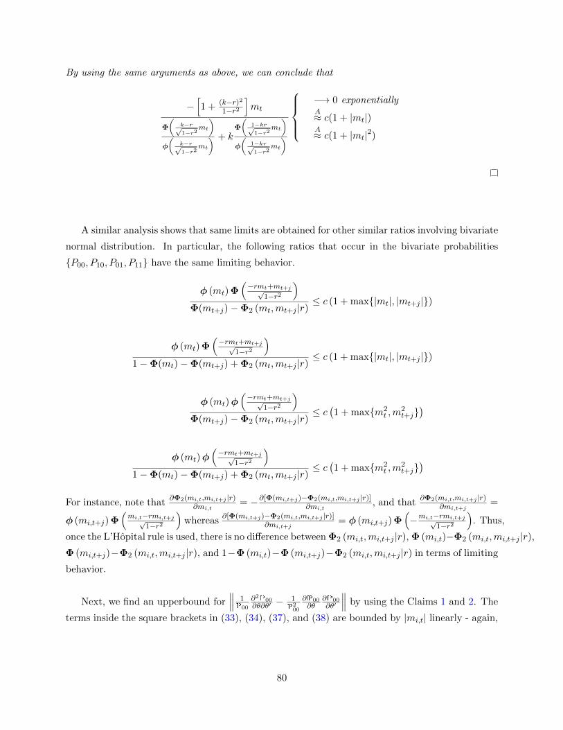
By using the same arguments as above, we can conclude that
−[1 + (k−r)2
1−r2
]mt
Φ
(k−r√1−r2
mt
)φ
(k−r√1−r2
mt
) + kΦ
(1−kr√1−r2
mt
)φ
(1−kr√1−r2
mt
)
−→ 0 exponentiallyA≈ c(1 + |mt|)A≈ c(1 + |mt|2)
A similar analysis shows that same limits are obtained for other similar ratios involving bivariate
normal distribution. In particular, the following ratios that occur in the bivariate probabilities
{P00, P10, P01, P11} have the same limiting behavior.
φ (mt) Φ(−rmt+mt+j√
1−r2
)Φ(mt+j)−Φ2 (mt,mt+j |r)
≤ c (1 + max{|mt|, |mt+j |})
φ (mt) Φ(−rmt+mt+j√
1−r2
)1−Φ(mt)−Φ(mt+j) + Φ2 (mt,mt+j |r)
≤ c (1 + max{|mt|, |mt+j |})
φ (mt)φ(−rmt+mt+j√
1−r2
)Φ(mt+j)−Φ2 (mt,mt+j |r)
≤ c(1 + max{m2
t ,m2t+j}
)
φ (mt)φ(−rmt+mt+j√
1−r2
)1−Φ(mt)−Φ(mt+j) + Φ2 (mt,mt+j |r)
≤ c(1 + max{m2
t ,m2t+j}
)For instance, note that
∂Φ2(mi,t,mi,t+j |r)∂mi,t
= −∂[Φ(mi,t+j)−Φ2(mi,t,mi,t+j |r)]∂mi,t
, and that∂Φ2(mi,t,mi,t+j |r)
∂mi,t+j=
φ (mi,t+j) Φ(mi,t−rmi,t+j√
1−r2
)whereas
∂[Φ(mi,t+j)−Φ2(mi,t,mi,t+j |r)]∂mi,t+j
= φ (mi,t+j) Φ(−mi,t−rmi,t+j√
1−r2
). Thus,
once the L’Hopital rule is used, there is no difference between Φ2 (mi,t,mi,t+j |r), Φ (mi,t)−Φ2 (mi,t,mi,t+j |r),Φ (mi,t+j)−Φ2 (mi,t,mi,t+j |r), and 1−Φ (mi,t)−Φ (mi,t+j)−Φ2 (mi,t,mi,t+j |r) in terms of limiting
behavior.
Next, we find an upperbound for∥∥∥ 1P00
∂2P00∂θ∂θ′ −
1P
200
∂P00∂θ
∂P00∂θ′
∥∥∥ by using the Claims 1 and 2. The
terms inside the square brackets in (33), (34), (37), and (38) are bounded by |mi,t| linearly - again,
80

I assume without loss of generality, |mi,t| ≥ |mi,t+j | and m2i,t ≥ m2
i,t+j .
∣∣∣∣∣−mi,t −r√
1− r2
φ(−rmi,t+mi,t+j√
1−r2
)Φ(−rmi,t+mi,t+j√
1−r2
) − φ (mi,t) Φ(−rmi,t+mi,t+j√
1−r2
)Φ2 (mi,t,mi,t+j |r)
∣∣∣∣∣ ≤ c(1 + |mi,t|)
∣∣∣∣∣−mi,t+j −r√
1− r2
φ(mi,t−rmi,t+j√
1−r2
)Φ(mi,t−rmi,t+j√
1−r2
) − φ (mi,t+j) Φ(mi,t−rmi,t+j√
1−r2
)Φ2 (mi,t,mi,t+j |r)
∣∣∣∣∣ ≤ c(1 + |mi,t|)
∣∣∣∣∣−mi,t − rmi,t+j√1− r2
−√
1− r2φ (mi,t) Φ
(−rmi,t+mi,t+j√
1−r2
)Φ2 (mi,t,mi,t+j |r)
∣∣∣∣∣ ≤ c(1 + |mi,t|)
∣∣∣∣∣−−rmi,t +mi,t+j√1− r2
−√
1− r2φ (mi,t+j) Φ
(mi,t−rmi,t+j√
1−r2
)Φ2 (mi,t,mi,t+j |r)
∣∣∣∣∣ ≤ c(1 + |mi,t|)
The term inside the square brackets in (35) is bounded by |mi,t| quadratically
∣∣∣∣∣r +mi,t − rmi,t+j√
1− r2
−rmi,t +mi,t+j√1− r2
−√
1− r2φ (mi,t)φ
(−rmi,t+mi,t+j√
1−r2
)Φ2 (mi,t,mi,t+j |r)
∣∣∣∣∣ ≤ c(1 +m2i,t)
The term inside the square brackets in (36) is finite
∣∣∣∣∣ 1√1− r2
−Φ(−rmi,t+mi,t+j√
1−r2
)φ(−rmi,t+mi,t+j√
1−r2
) φ (mi,t+j) Φ(mi,t−rmi,t+j√
1−r2
)Φ2 (mi,t,mi,t+j |r)
∣∣∣∣∣ <∞Therefore, we can conclude that the norm of (29) is bounded by
∥∥∥ 1
P00
∂2P00
∂θ∂θ′− 1
P200
∂P00
∂θ
∂P00
∂θ′
∥∥∥ ≤ ∥∥∥∂2mi,t
∂θ∂θ′
∥∥∥c(1 + |mi,t|)
+∥∥∥∂2mi,t+j
∂θ∂θ′
∥∥∥c(1 + |mi,t|)
+∥∥∥ ∂2r
∂θ∂θ′
∥∥∥c(1 + |mi,t|)
+∥∥∥∂mi,t
∂θ
∂mi,t
∂θ′
∥∥∥c(1 +m2i,t)
+∥∥∥∂mi,t+j
∂θ
∂mi,t+j
∂θ′
∥∥∥c(1 +m2i,t)
+∥∥∥∂r∂θ
∂r
∂θ′
∥∥∥c(1 +m4i,t)
+∥∥∥∂mi,t
∂θ
∂mi,t+j
∂θ′+∂mi,t+j
∂θ
∂mi,t
∂θ′
∥∥∥c(1 +m2i,t)
+∥∥∥∂mi,t
∂θ
∂r
∂θ′+∂r
∂θ
∂mi,t
∂θ′
∥∥∥c(1 + |mi,t|3)
+∥∥∥∂mi,t+j
∂θ
∂r
∂θ′+∂r
∂θ
∂mi,t+j
∂θ′
∥∥∥c(1 + |mi,t|3)
81

Arranging the terms yields
∥∥∥ 1
P00
∂2P00
∂θ∂θ′− 1
P200
∂P00
∂θ
∂P00
∂θ′
∥∥∥≤ c(1 + |mi,t|)
(∥∥∥∂2mi,t
∂θ∂θ′
∥∥∥+∥∥∥∂2mi,t+j
∂θ∂θ′
∥∥∥+∥∥∥ ∂2r
∂θ∂θ′
∥∥∥)+ c(1 +m2
i,t)
(∥∥∥∂mi,t
∂θ
∂mi,t
∂θ′
∥∥∥+∥∥∥∂mi,t+j
∂θ
∂mi,t+j
∂θ′
∥∥∥+∥∥∥∂mi,t
∂θ
∂mi,t+j
∂θ′
∥∥∥+∥∥∥∂mi,t+j
∂θ
∂mi,t
∂θ′
∥∥∥)+ c(1 + |mi,t|3)
(∥∥∥∂mi,t
∂θ
∂r
∂θ′
∥∥∥+∥∥∥∂r∂θ
∂mi,t
∂θ′
∥∥∥+∥∥∥∂mi,t+j
∂θ
∂r
∂θ′
∥∥∥+∥∥∥∂r∂θ
∂mi,t+j
∂θ′
∥∥∥)+ c(1 +m4
i,t)∥∥∥∂r∂θ
∂r
∂θ′
∥∥∥A similar analysis not shown here indicates that the same upperbound is found for the other three
norms∥∥∥ 1Pkl
∂2Pkl∂θ∂θ′ −
1P
2kl
∂Pkl∂θ
∂Pkl∂θ′
∥∥∥ for {k, l} ∈ {0, 1}.
B.3 Bounds on functions of mt(θ)
In this subsection, I analyze the upperbounds for functions of mi,t(θ), in particular the bounds for
mi,t,m2i,t,m
′i,t. First, remember that mi,t(xi, θ) =
√1− ρ2
∑tk=0 ρ
kβ′xi,t−k.
The bound for mi,t(θ) is
|mi,t(θ)| =∣∣∣√1− ρ2
t∑k=0
ρkβ′xi,t−k
∣∣∣ ≤√1− ρ2
t∑k=0
|ρkβ′xi,t−k| ≤t∑
k=0
|ρ|k‖β‖‖xi,t−k‖
The bound for m2i,t(θ) is
m2i,t(θ) =
(√1− ρ2
t∑k=0
ρkβ′xi,t−k
)2
= (1− ρ2)
t∑k=0
t∑l=0
ρk+lβ′xi,t−kx′i,t−lβ
≤ (1− ρ2)∣∣∣ t∑k=0
t∑i=0
ρk+lβ′xi,t−kx′t−iβ
∣∣∣≤ (1− ρ2)
t∑k=0
t∑i=0
|ρ|k+l∣∣β′xi,t−kx′t−iβ∣∣
≤t∑
k=0
t∑l=0
|ρ|k+l‖β‖2‖xi,t−k‖‖xi,t−l‖
82

The first derivative of mi,t(θ) is
∂mi,t(θ)
∂θ′= −
t∑k=0
∂(√
1− ρ2ρkβ′xi,t−k
)∂ρ
,∂(√
1− ρ2ρkβ′xi,t−k
)∂β′
= −
t∑k=0
[(−ρ√1− ρ2
ρk +√
1− ρ2kρk−1
)β′xi,t−k,
√1− ρ2ρkx′i,t−k
]
= −√
1− ρ2
t∑k=0
[(−ρ2
1− ρ2+ k
)ρk−1β′xi,t−k, ρkx′i,t−k
]
Next, let’s write the norm of the derivative.
∥∥∥∂mi,t(θ)
∂θ′
∥∥∥ ≤ t∑k=0
∥∥∥∥∥[(−ρ2
1− ρ2+ k
)ρk−1β′xi,t−k, ρkx′i,t−k
]∥∥∥∥∥≤
t∑k=0
∣∣∣∣∣(−ρ2
1− ρ2+ k
)ρk−1β′xi,t−k
∣∣∣∣∣+
t∑k=0
∥∥ρkx′i,t−k∥∥≤
t∑k=0
(ρ2
1− ρ2+ k
)|ρ|k−1‖β‖‖xi,t−k‖+
t∑k=0
|ρ|k‖xi,t−k‖
Hence, supθ∈Θ
∥∥∥∂mi,t(θ)∂θ
∥∥∥ ≤M∑tk=0(1 + k)ρk‖xi,t−k‖.
The second derivative of mi,t(θ) is
∂mi,t(θ)
∂θ∂θ′= −
t∑k=0
(− 2k+1√
1−ρ2ρk − ρk+2
√1−ρ2
3 +√
1− ρ2k(k − 1)ρk−2
)β′xi,t−k
∂2mi,t∂ρ∂β′(
−ρ√1−ρ2
ρk +√
1− ρ2kρk−1
)xi,t−k 0
Hence, supθ∈Θ
∥∥∥∂mi,t(θ)∂θ∂θ′
∥∥∥ ≤M∑tk=0(1 + k2)ρk‖xi,t−k‖.
83
Related Documents