composing timbre spaces - Stacks are the Stanford

COMPOSING TIMBRE SPACES, COMPOSING TIMBRE IN SPACE:

AN EXPLORATION OF THE POSSIBILITIES OF MULTIDIMENSIONAL TIMBRE REPRESENTATIONS AND THEIR COMPOSITIONAL APPLICATIONS

A FINAL PROJECTSUBMITTED TO THE DEPARTMENT OF MUSIC

AND THE COMMITTEE ON GRADUATE STUDIES OF STANFORD UNIVERSITY

IN PARTIAL FULFILLMENT OF THE REQUIREMENTS FOR THE DEGREE OF

DOCTOR OF MUSICAL ARTS

Leah Christinne Reid June 2013

http://creativecommons.org/licenses/by-nc/3.0/us/

This dissertation is online at: http://purl.stanford.edu/kp339nk6272

Includes supplemental files:

1. Original size 11 x 17 score of Ostiatim (Reid_Ostiatim_Score.pdf)

2. Original size 11 x 17 score of Clocca (Reid_Clocca_Score.pdf)

3. Original size 11 x 17 score of Occupied Spaces (Reid_Occupied_Spaces_Score.pdf)

4. Recording of Ostiatim (Reid_Ostiatim_Recording.mp3)

5. Recording of Clocca (Reid_Clocca_Recording 3.mp3)

6. Recording of Occupied Spaces (Reid_Occupied_Spaces_Recording.mp3)

© 2013 by Leah Christinne Reid. All Rights Reserved.

Re-distributed by Stanford University under license with the author.

This work is licensed under a Creative Commons Attribution-Noncommercial 3.0 United States License.

ii

I certify that I have read this dissertation and that, in my opinion, it is fully adequatein scope and quality as a dissertation for the degree of Doctor of Musical Arts.

Mark Applebaum, Primary Adviser

I certify that I have read this dissertation and that, in my opinion, it is fully adequatein scope and quality as a dissertation for the degree of Doctor of Musical Arts.

Jonathan Berger

I certify that I have read this dissertation and that, in my opinion, it is fully adequatein scope and quality as a dissertation for the degree of Doctor of Musical Arts.

Brian Ferneyhough

I certify that I have read this dissertation and that, in my opinion, it is fully adequatein scope and quality as a dissertation for the degree of Doctor of Musical Arts.

Jaroslaw Kapuscinski

Approved for the Stanford University Committee on Graduate Studies.

Patricia J. Gumport, Vice Provost Graduate Education

This signature page was generated electronically upon submission of this dissertation in electronic format. An original signed hard copy of the signature page is on file inUniversity Archives.

iii

ABSTRACT

This final project is comprised of three works completed over the past two years,

and an introductory paper that briefly outlines the approaches to timbre taken in each

piece. All three of the compositions approach timbre from a different perspective and

explore the possibilities and compositional applications of multidimensional timbre

representations. The final project does not present a comprehensive history of timbre, all

the research that has been undertaken on the topic, or a complete account of the

composers who have used timbre models. Rather, the models and compositions presented

here are meant to provide insight into my own compositional thought process. The three

original pieces illustrate a trajectory through which composing with timbre yielded new

creative insights and compositional techniques. Emergent in these works is a common

theme and exploration of “timbre space” and “timbre in space.”

The first piece presented in this portfolio is Ostiatim, for string quartet. It explores

timbre space as a morphing device for sculpting material. Ostiatim was premiered by the

Jack Quartet.

The second piece, Clocca, for chamber ensemble, examines timbre space as a

structuring device. Clocca was premiered by the Talea Ensemble.

Finally, the third piece in the collection, Occupied Spaces, for two piano and

percussion, explores a series of timbral spaces, presented as “rooms,” which grow, shrink,

and continuously shift in shape. Unlike Ostiatim and Clocca, this final piece explores

timbre in space. Occupied Spaces was premiered by the ensemble Yarn/Wire.

iv

TABLE OF CONTENTS

v

List of Figures

List of Supplemental Materials

Acknowledgements

I. Introduction 1.1 What is Timbre?

1.1.1 Timbral Parameters 1.1.2 What is a Timbre Space?

1.2 Select Timbre Models and Their Compositional Applications 1.2.1 Pollard & Janson (1982) 1.2.2 Grey (1977) and McAdams et al. (1995)

1.3 The Temporality of Timbre 1.4 Timbre Models in Select Compositions

1.4.1 Krystof Penderecki: Classification and Timbral Categories 1.4.2 Mathias Spahlinger’s Timbre Space 1.4.3 Kaija Saariaho’s “Timbral Axis”

1.5 Timbre Models in My Music

II. Ostiatim 2.1 Introduction 2.2 Form 2.3 Timbre as a Morphing Device

III. Clocca 3.1 Introduction 3.2 Form: Timbre as a Structuring Device 3.3 Treatment of Time

IV. Occupied Spaces 4.1 Introduction 4.2 Form 4.3 Eleven Rooms: Timbre in Space

V. Summary and Conclusions

VI. Scores 6.1 Score for Ostiatim 6.2 Score for Clocca 6.3 Score for Occupied Spaces

Bibliography

vi

vii

viii

1 1 2 334 510131417 1921

24242626

3131 3238

39394043

57

595971

106

154

LIST OF FIGURES

vi

568

1012151820222527282930323335373741424244

46-4748-52

Figure 1 — Diagram of Pollard & Janson’s tristimulus model (1982) Figure 2 — Grey’s timbre space (1977) Figure 3 — McAdams et al.’s timbre space (1995) Figure 4 — Proposed compositional application of Grey’s timbre space Figure 5 — Musique Concrète diagram Figure 6 — Pairs of materials in Penderecki’s timbre system Figure 7 — Timbre space from Spahlinger’s 128 erfüllte augenblicke Figure 8 — Saariaho’s “timbral axis” Figure 9 — Timbre spaces used in my own works Figure 10 — Anish Kapoor’s Memory Figure 11 — Ostiatim’s Form Figure 12 — Timbre cubes as they relate to Ostiatim Figure 13 — Ostiatim’s Fragment 1—points in space for cubes 1 and 2 Figure 14 — Ostiatim’s Fragment 2—trajectories in space for cubes 1 and 2 Figure 15 — Analysis of Clocca’s bell sound illustrating 37 partials and their cut-offs Figure 16 — Partial numbers and cutoff times for the bell sound Figure 17 — Structural partials and gradual distortion of spectra in Clocca Figure 18 — Graphical illustration of Clocca’s structural partials Figure 19 — Graphical depiction of Clocca’s block structures Figure 20 — Example of Occupied Spaces two-part theme Figure 21 — Spectrogram and graphical representation of Occupied Spaces’ form Figure 22 — Graphical illustration of the temporal room spatialization Figure 23 — Frequencies of the largest bands for sections 1-5 Figure 24 — Original analyses of rooms on the pitch B4 Figure 25 — Orchestration of rooms

SUPPLEMENTAL MATERIALS

Recording of Ostiatim — performed by the Jack Quartet, 2011Recording of Clocca — performed by the Talea Ensemble, 2012Recording of Occupied Spaces — performed by Yarn/Wire, 2013Original size 11 x 17 score of OstiatimOriginal size 11 x 17 score of CloccaOriginal size 11 x 17 score of Occupied Spaces

vii

ACKNOWLEDGEMENTS

I wish to thank my primary adviser Mark Applebaum and advisors Jonathan

Berger, Brian Ferneyhough, and Jaroslaw Kapuscinski for their invaluable insight,

support, and guidance throughout my time at Stanford University. Thanks also goes to

Sean Ferguson from McGill University, who first opened my ears to the world of timbre.

Special gratitude goes to my parents, Christinne and Ronald Reid, and my

husband, James DeMuth, for their unwavering support and encouragement. This final

project is dedicated to them.

viii

I. INTRODUCTION

“The whole of our sound world is available for music-mode listening, but it probably takes a catholic taste and a well-developed interest to find jewels in the auditory garbage of machinery, jet planes, traffic, and other mechanical chatter that constitute our sound environment. Some of us, and I confess I am one, strongly resist the thought it is garbage. The more one listens the more one finds that it is all jewels.”

—Robert Erickson, Sound Structure in Music (1975, p.1)

1.1 What is Timbre?

Timbre is a complex dimension of auditory perception. Its definition is elusive.

The most widely used definition of timbre, that of The American National Standards

Institute (1960) describes the term as “that attribute of auditory sensation in terms of

which a listener can judge two sounds...having the same loudness and pitch as

dissimilar”—in effect, a definition based on what is excluded from the term. Unlike pitch

and loudness there is no simple, objective, or single dimensional scale that describes this

phenomenon (Rossing, 1990). Timbre can, however, be described as a multidimensional

attribute of sound, where many physical aspects correlate with perceptual dimensions

pertaining to “spectral, temporal, and spectrotemporal properties of sound

events” (McAdams, 2006).

As timbre became increasingly central in my composition, I adopted a hybrid

model that integrates both the “color” and “texture” of sound, and incorporates both static

and dynamic attributes of timbre. The “color” of sound is described in terms of an

“instantaneous snapshot of the spectral envelope,” while the “texture” of a sound

describes the “the sequential changes in color with an arbitrary time scale” (as cited in

Rossing, 2012). This view of timbre has been developed at CCRMA by Hiroko Terasawa

1

and Professor Jonathan Berger, and hints at two important compositional elements in a

piece: 1) static, vertical pitch and chordal structures, and 2) dynamic, horizontal temporal

processes. While these elements are important, this definition is still rather vague as to

the descriptive factors of timbre. In order to better understand how to compose with

timbre it becomes necessary to view the physical parameters associated with timbre

perception.

1.1.1 Timbral Parameters

The multidimensionality and complexity of timbre is best illustrated by the

following list from Traube’s lecture “Instrumental and Vocal Timbre Perception” (2006):

- Temporal Envelope- Spectral Envelope- Absolute Frequency Position of Spectral Envelope- Variations of Harmonic Contents- Position of Spectral Centroid, or rather the brightness or sharpness of a sound- Harmonic and Noise Components Ratio- Inharmonic Ratio- Odd/Even Harmonic Ratio- Synchronicity of Partials- Onset Effects:

- Rise time, presence of noise or inharmonic partials during onset, unequal rise of partials, characteristic shape of rise curves

- Steady State Effects: - Vibrato, amplitude modulation, gradual swelling, pitch instability

Traube’s list notably focuses on the overall spectrum, as well as the dynamic features of

individual components. These parameters begin to give one a better idea of what timbre

actually is, but they still do not give a full view of how these parameters interact or

provide a basis for one to compose with timbre. This is where a spatial or geometric

model of timbre is beneficial.

2

1.1.2 What is a Timbre Space?

The complexity of timbre is clear when one attempts to visually represent it in

space. Since the 1970s, many multidimensional perception studies have been conducted,

and researchers have tackled timbre’s dimensions from various angles to find the best

descriptive words to characterize them. These multidimensional “spaces” are commonly

referred to as timbre spaces. A timbre space is “a model that predicts the perceptual

results such as auditory stream formation, [and] timbral interval perception” (McAdams,

2006). Depending on the stimuli tested, different correlates are produced. For example,

Lakatos’ study in 2000 included recorded wind, string, percussion, and combined sounds;

Grey’s 1977 study used recorded and modified instrument tones; Iverson & Krumhansl’s

1993 study used attack and remainder portions of tones; and McAdams’ 1995 study used

FM-synthesized simulations of orchestral instrument tones. The aim of these studies is to

“find robust descriptors that explain perceptual data across studies, [to] develop

perceptually relevant acoustic distance models for measuring similarity objectively, [and

to] find powerful descriptors for sound categorization and source identification”

(McAdams, 2006). The understanding of these descriptive terms, spaces, and their

dimensions offer perspective on how timbre should be treated in a compositional model.

1.2 Select Timbre Models and Their Compositional Applications

There are many timbre models worth studying in the pursuit of understanding

timbre. While I will not go into detail about every timbre model in the literature, for the

purpose of this project I will examine three classic timbre models and their possible

3

compositional applications: Pollard and Janson’s tristimulus model, and both Grey’s and

McAdams’ timbre spaces. Here is a list of some of the other models I have found

particularly useful: Singh & Woods (1970), Pratt & Doak (1976), Von Bismark (1974),

Grey & Gordon (1978), Wessel (1979), Krumshansl (1989), Iverson & Krumshansl

(1993), Lakatos (2000), and Peterson & Barney (1952). While the examination of these

and other timbre spaces is useful for cultivating a definition of timbre, the real question

for me is how does one use timbre as a compositional model?

1.2.1 Pollard & Janson (1982)

The first model, Pollard and Janson’s tristimulus method (1982), was inspired by

the RGB color model developed in the world of visual perception. The RGB color model

describes the way three primary colors—red, green, and blue—can be mixed to create an

infinitely broad array of colors. The musical tristimulus model is a timbre descriptor that

measures the mixture of harmonics in a given sound in three bands. The first band, or

tristimulus, measures the relative weight—or rather amplitude—of the fundamental of the

sound; the second measures the relative weight of the second, third, and fourth mid-

frequency harmonics; and the third measures the relative weight of the remaining high-

frequency harmonics. The model is often arranged in a triangular space where the three

dimensions meet in a single point. The corners represent the maximum values of each

band. This model in itself represents a steady state spectrum and was specifically

designed to analyze the timbre of a single tone. While it lacks a representation of time,

one can convert the tristimulus model into a temporal model by imposing a trajectory

within the space. A diagram of the tristimulus model can be seen in figure 1.

4

The tristimulus model could potentially inform compositional decisions both by

selecting (either algorithmically or arbitrarily) points within the space, as well as

imposing trajectories between multiple points. At each point, a different ratio of the

fundamental to upper partials is possible. Therefore, one could develop a timbral

“harmonic” progression in which particular partials are highlighted and emphasized while

the fundamental stays the same. The tristimulus model is, conceptually, a framework for

additive synthesis in that the position in the space dictates the respective ratios of

amplitudes of the fundamental, low-order, and higher partials. Additive synthesis has

been extremely important in the works of spectral composers.1

1.2.2 Grey (1977) and McAdams et al. (1995)

Next, I will briefly discuss both Grey’s 1977 and McAdams’ 1995 timbre spaces.

In the former, Grey analyzed sixteen instrument tones and created computer synthesized

5

1 “[Additive synthesis] creates complex sounds by combining simple sounds with different amplitudes. The mixture stops on organs are the oldest form of additive synthesis” (Fineberg, 2000, p.111). An example of additive synthesis used in a composition can be seen in Gerard Grisey’s Partiels.

Figure 1. Diagram of Pollard & Janson’s tristimulus model. Adapted from “A Tristimulus Method for the Specification of Musical Timbre,” by H.F. Pollard and E.V. Janson, 1982, International Journal of Acoustics, 51, p.166.

stimuli with equal pitch, loudness, and subjective duration. Listeners rated the

dissimilarities for all pairs of tones (Grey, 1977). The resulting timbre space can be

viewed in figure 2. The first dimension, labeled brightness, represents the spectral

envelope of the sound. Brighter sounds are seen at the bottom of the cube. For example, a

sound that has “low brightness” would be a French horn or a violoncello playing sul

tasto. In contrast, a sound that had “high brightness” on this scale would be an oboe or a

muted trumpet (Traube, 2006).

Dimension 2 represents the spectral flux of the sound and explains how the sound

evolves over time. In this model, the greater the flux, the more to the right of the cube it

appears. “This dimension is related to a combination of the degree of fluctuation in the

spectral envelope and the synchronicity of onsets of the different harmonics” (Traube,

2006). To illustrate, sounds that have high synchronicity and low fluctuation are clarinet

6

Figure 2. Grey’s timbre space. Reproduced and altered in “Instrumental and Vocal Timbre Perception,” by C. Traube, 2006; adapted from “Multidimensional Perceptual Scaling of Musical Timbres,” by J. M. Grey, 1977, Journal of the Acoustical Society of America, 61.

and saxophone; sounds that have low synchronicity and high fluctuation are flute and

violoncello (Traube, 2006).

The third dimension, labeled as transients density, “represents the degree of

presence of the attack transients” (Traube, 2006). Examples of sounds with more

transients include: strings, flute, and single reed instruments such as clarinet and

saxophone. Examples of sounds that have fewer transients are: brass, bassoon, and

English horn (Traube, 2006).

McAdams’ timbre space is essentially a verification of Grey’s studies and can be

viewed in figure 3. In this study, “McAdams and his colleagues (1995) employed

eighteen FM timbres, including both instrument imitations and hybrids... Dissimilarity

ratings were made on a nine point scale, with nine being ‘very dissimilar’” (McAdams,

2011, p.88). The experiment selected a three-dimensional model with attack time,

spectral centroid, and spectral flux. The first dimension is labeled rise or attack time,

which is essentially the same as transients density; the second is spectral centroid, which

is equivalent to brightness; and the third is spectral flux (which is labeled the same in

Grey’s study) (McAdams et al., 1995).

Both of these models were created using a technique called multidimensional

scaling (MDS) which is a statistical technique used for data visualization. MDS is a tool

that studies “(dis)similarity” ratings, reveals relationships, and then maps them into a

geometric space (McAdams, 1995). They are then interpreted by an investigator that

“...attempts to interpret the configuration with regard to factors which may explain the

ordering of points along the various axes, or dimensions, of the space” (Grey, 1977, p.

7

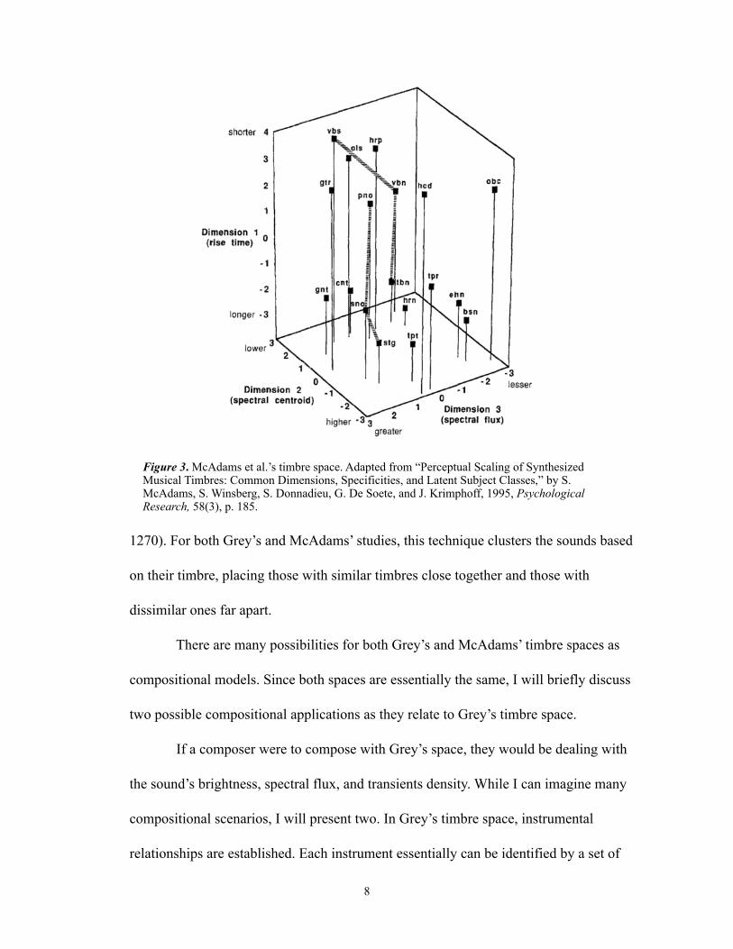
1270). For both Grey’s and McAdams’ studies, this technique clusters the sounds based

on their timbre, placing those with similar timbres close together and those with

dissimilar ones far apart.

There are many possibilities for both Grey’s and McAdams’ timbre spaces as

compositional models. Since both spaces are essentially the same, I will briefly discuss

two possible compositional applications as they relate to Grey’s timbre space.

If a composer were to compose with Grey’s space, they would be dealing with

the sound’s brightness, spectral flux, and transients density. While I can imagine many

compositional scenarios, I will present two. In Grey’s timbre space, instrumental

relationships are established. Each instrument essentially can be identified by a set of

8

Figure 3. McAdams et al.’s timbre space. Adapted from “Perceptual Scaling of Synthesized Musical Timbres: Common Dimensions, Specificities, and Latent Subject Classes,” by S. McAdams, S. Winsberg, S. Donnadieu, G. De Soete, and J. Krimphoff, 1995, Psychological Research, 58(3), p. 185.

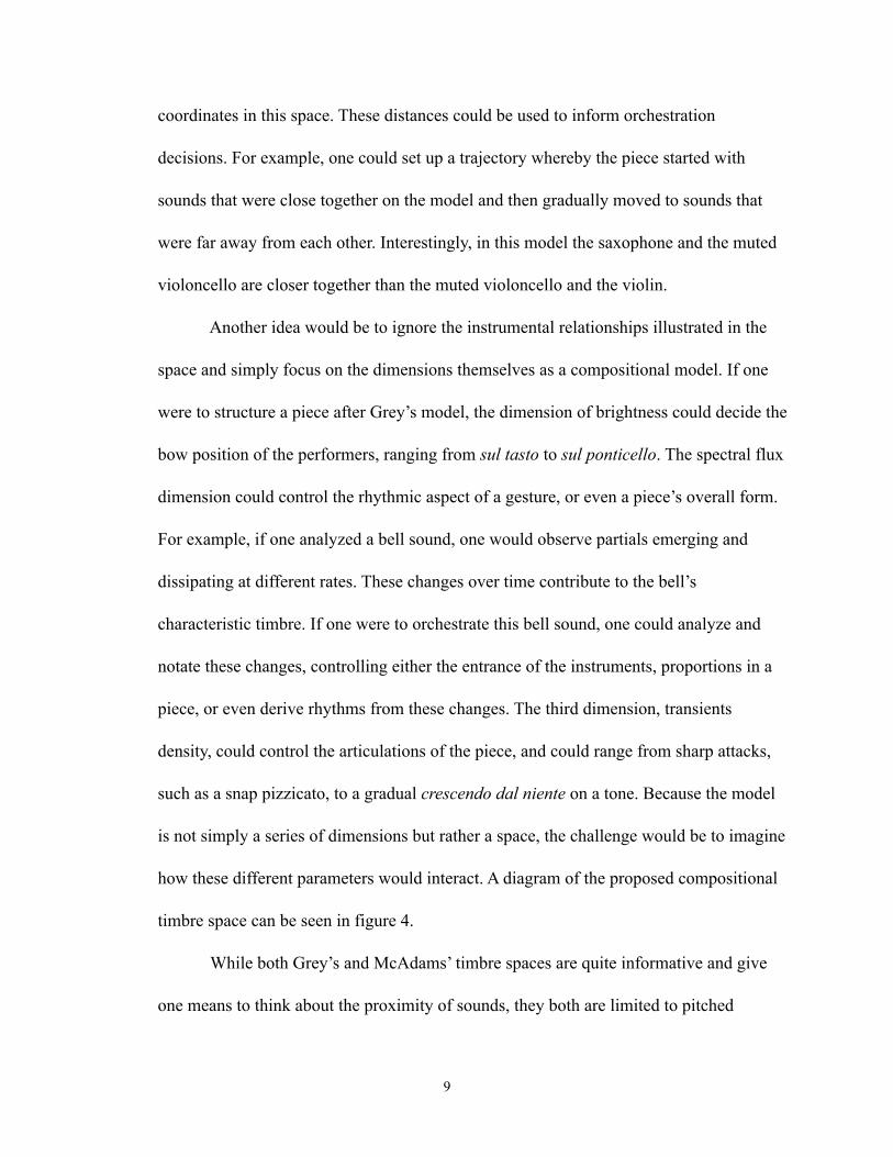
coordinates in this space. These distances could be used to inform orchestration

decisions. For example, one could set up a trajectory whereby the piece started with

sounds that were close together on the model and then gradually moved to sounds that

were far away from each other. Interestingly, in this model the saxophone and the muted

violoncello are closer together than the muted violoncello and the violin.

Another idea would be to ignore the instrumental relationships illustrated in the

space and simply focus on the dimensions themselves as a compositional model. If one

were to structure a piece after Grey’s model, the dimension of brightness could decide the

bow position of the performers, ranging from sul tasto to sul ponticello. The spectral flux

dimension could control the rhythmic aspect of a gesture, or even a piece’s overall form.

For example, if one analyzed a bell sound, one would observe partials emerging and

dissipating at different rates. These changes over time contribute to the bell’s

characteristic timbre. If one were to orchestrate this bell sound, one could analyze and

notate these changes, controlling either the entrance of the instruments, proportions in a

piece, or even derive rhythms from these changes. The third dimension, transients

density, could control the articulations of the piece, and could range from sharp attacks,

such as a snap pizzicato, to a gradual crescendo dal niente on a tone. Because the model

is not simply a series of dimensions but rather a space, the challenge would be to imagine

how these different parameters would interact. A diagram of the proposed compositional

timbre space can be seen in figure 4.

While both Grey’s and McAdams’ timbre spaces are quite informative and give

one means to think about the proximity of sounds, they both are limited to pitched

9

instrument sounds and thus omit any sound with a noise spectrum. Since noise is an

important parameter in contemporary music, any compositional timbre model would need

to address this crucial dimension.

1.3 The Temporality of Timbre

Timbre representation is typically rooted in Fourier analysis which describes a

discrete spectral slice solely in the frequency domain. By piecing these discrete

“snapshots” sequentially we can create a representation in the time-domain (this is called

a spectrogram). As previously mentioned, the perception of timbre has both “static” and

“temporal” aspects. To illustrate, I will reduce a few perceptual studies down to their

basic forms, representing only their title, year, and dimensions (McAdams, 2006):

10

Figure 4. Proposed compositional application of Grey’s timbre space.

- Grey & Gordon (1978)- Dimension 1 = Spectral centroid- Dimension 2 = Attack synchronicity/spectral flux - Dimension 3 = Attack centroid

- Krumhansl (1989)- Dimension 1 = Attack time - Dimension 2 = Spectral centroid - Dimension 3 = Spectral deviation

- McAdams et al. (1995)- Dimension 1 = Attack time - Dimension 2 = Spectral centroid - Dimension 3 = Spectral flux

As is the case with most perceptual timbre models, all of the studies listed above have at

least one dimension that describes the “brightness” of the sound (spectral centroid), and

one dimension that describes the sound’s temporal nature (spectral flux, attack

synchronicity, spectral deviation, and attack time). One can view a sound’s

transformation over time in sonograms.

Because our perception of timbre has a temporal element it is important to

understand how the envelope of a sound works. Each sound has a beginning, middle, and

end, or rather an attack, sustain, and decay. The attack portion of a signal envelope traces

the sound signal from zero intensity to its maximum amplitude; the steady state is the

portion of the signal that remains fairly constant; and the decay is the portion of the

envelope that traces the drop in amplitude to zero (Vassilakis, 1995). The temporal shape

of an envelope plays an important role in defining the timbre of a sound. Understanding

how the three “sections” of a sound work is essential for composing with timbre as a

compositional model.

In Musique Concrète, Pierre Schaeffer made use of these elements in his

compositions. To illustrate, figure 5 elegantly depicts a possible solution for how timbre

11

and time could interact. In Schaeffer’s system, the “Plan mélodique ou des tessitures

[describes] the evolution of pitch parameters with respect to time...[the] Plan dynamique

ou des formes [outlines] the evolution of intensity parameters with respect to time...[and

the] Plan harmonique ou des timbres [describes] the reciprocal relationship between the

parameters of pitch and intensity represented as a spectrum analysis” (Manning, 2013, p.

30-31). For more information on his studies of the nature and inner structure of sounds

defined in the concept of the object sonore, I refer the reader to his informative book:

Traité des objets musicaux (1966).

If one were to center a composition around timbre, at the bare minimum one

would have to define how the static and temporal components of the piece were

behaving. There are many ways to approach this. For example, one could model a piece

on an already existing sound, such as a bell tone or a clarinet’s multiphonic. An example

of such a work is Jonathan Harvey’s Mortuos Plango, Vivos Voco. In this piece Harvey

12

Figure 5. Musique Concrète diagram. Adapted from Electronic and Computer Music (p.31), by P. Manning, 2013, New York: Oxford University Press.

used the spectrum of a bell tone and sound of the singing voice of a boy. The composition

has eight sections that are set around eight pitches from the bell’s spectrum. In this piece

Harvey transforms one bell sound to another through glissandi and a pivot through a

center tone. The eight spectra of the piece are static snapshots of sound, and the temporal

elements of the piece are the transformations and modulations between these snapshots

(Harvey, 1981).

While understanding that timbre has both static and temporal elements is

important, the composer also needs to master the understanding and manipulation of the

perception of time. As Julio D’Escrivan’s surmised in his article “Reflections on the

Poetics of Time in Electroacoustic Music,” time becomes a poetic element. The composer

can “speed up” or “slow down” time. The experience of time can be subjective and

people often perceive that time has different “speeds.” This subjectivity of time has to do

with the psychological state of the listener (1989). As noted in Philippe Manoury’s paper

“The Arrow of Time,” pleasant experiences seem to move by “too quickly” while

boredom seems to make time “slow down.” These variations in state gives one the

concept of form (Manoury, 1984).2

1.4 Timbre Models in Select Compositions

I have been influenced by many different works, composers, and theorists,

including: Gérard Grisey, Tristain Murail, Joshua Fineberg, Jonathan Harvey, Arnold

Schoenberg, Olivier Messiaen, Claude Debussy, Wayne Slawson, Fred Lerdahl, Robert

13

2 A more extensive description of this process can be found in Grisey’s “Tempus ex Machina: a Composer’s Reflection on Musical Time.”

Cogan, Edgard Varèse, Helmut Lachenmann, Harry Partch, Pierre Henri, Herbert Eimert,

Luc Ferrari, La Monte Young, George Crumb, Luigi Nono, Gyorgy Ligeti, Anton

Webern, Philippe Manoury, Andre Dalbavie, John Cage, Jean-Claude Risset, and Claude

Vivier, to name a few. However, there are not many composers that make timbre the

primary concern in their works. While the first composers that may come to mind are

from the spectral school, notably Grisey and Murail, the timbral systems of Krystof

Penderecki, Mathias Spahlinger, and Kaija Saariaho are particularly compelling. Timbre

is of primary importance in their music and manifests itself in every aspect of the

compositional process, from pitch to form. Their systems seem to resonate most strongly

with my current exploration of timbre. I will briefly present their models and explain my

interest.

1.4.1 Krystof Penderecki: Classification and Timbral Categories

Penderecki’s approach to timbre in the early sixties was inspired by Drobner’s

book Instrumentoznawstwo i akustyka, a classic Polish handbook for organology and

acoustics. Penderecki studied the ways sounds were generated and understood timbre

primarily as a function of materials that were employed in the process of sound

generation. In his book, Drobner labeled the sound source a vibrator and the body which

agitates the vibrator an inciter. The combination of the two is a sound generator. This

terminology became a point of departure for a timbre organization system elaborated by

Penderecki in eight of his pieces written between 1960-1962: Anaklasis for 42 strings and

percussion; Threnody—To the Victims of Hiroshima for 52 strings; String Quartet No. 1;

Dimensions of Time and Silence for mixed choir, strings, and percussion; Fonogrammi

14

for flute and chamber orchestra; Polymorphia for 48 strings; Fluorescences for orchestra;

and Canon for string orchestra and tape (Mirka, 2001).

In his system, Penderecki derived timbral categories based upon materials most

commonly used in the construction of musical instruments and accessories, including

metal, wood, leather, felt, and hair. All of these materials can serve as both vibrators and

inciters. However, for practical reasons, while the role of inciter can be played by any of

the listed materials, the vibrator can only be made of metal, wood, or leather. These three

sounding bodies become primary material categories and can interact with any material,

including themselves. Hair and felt, on the other hand, never interact with each other or

itself within Penderecki’s system (Mirka, 2001).

The matrix in figure 6 illustrates the possible pairs of interacting materials. Every

pair in the diagram indicates one type of sound generator as well as the type of timbre

characteristic of sounds generated by it (Mirka, 2001).

15

Figure 6. Pairs of materials in Penderecki’s timbre system. Adapted from “To Cut the Gordian Knot: The Timbre System of Krysztof Penderecki,” by D. Mirka, 2001, Journal of Music Theory, 45(2), p. 437.

While the system explains the individual categories of sounds used in

Penderecki’s music, it does not explain how these sounds interact. Penderecki solved this

problem by grouping sounds together into sets which he called segments. Generators in

the segments often featured the same principle material which was excited in different

ways. For example, if the main material in a segment was wood then it could be excited

by metal, leather, or hair. Segments therefore became defined based on their main

materials and can be viewed as the elementary building blocks of the composition

(Mirka, 2001).

Penderecki’s timbre system controls both the morphology and the succession of

segments throughout a piece. The eight pieces that were written using this system are

structured around the timbral oppositions between metal, wood, and leather as primary

materials. These opposing timbral poles provide the overarching structural components

for a piece. For example, if a segment whose main material is wood is followed by a

metal segment, one will perceive a timbral opposition. These poles can also be treated

transitionally, and one timbre can gradually morph into another one (Mirka, 2001).

While Penderecki only used this timbre system for three years, from 1960-1962, it

offers a great insight into his view of timbre. This system fascinates me because

Penderecki essentially created a lexicon of all possible sounds and structured his pieces

based around these choices. In my own model, I similarly make exhaustive lists of the

sounds that can be created by the available instruments and group them based on pre-

defined qualities. While I do not use material classification as the basis for my timbre

16

system, the process of categorization, creation of poles, and morphing between these

poles is quite similar.

1.4.2 Mathias Spahlinger’s Timbre Space

Spahlinger’s 128 erfüllte augenblicke is an example of a piece that uses a

compositional timbre space model as a formal structuring device. The piece itself consists

of 128 one-page pieces for soprano, clarinet in B-flat, and violoncello. The performers

are in charge of choosing both the pieces that they will perform (because not all 128 need

be played) and the order in which they will perform them. They can repeat each piece

freely and separate them by any duration of pauses. If all 128 pieces were played

consecutively with only brief pauses between them, the resulting duration would be

approximately one hour. Each piece is labeled by a three-digit code and an inequality

symbol. The code indicates the piece’s position in a three-dimensional matrix printed in

the preface to the score. The three numbers of the code represent the specific location of

the piece in the structure. The inequality symbols—given as either an increase (<) or

decrease (>) sign—show the piece’s tendencies across unspecified dimensions (Blume,

2008).

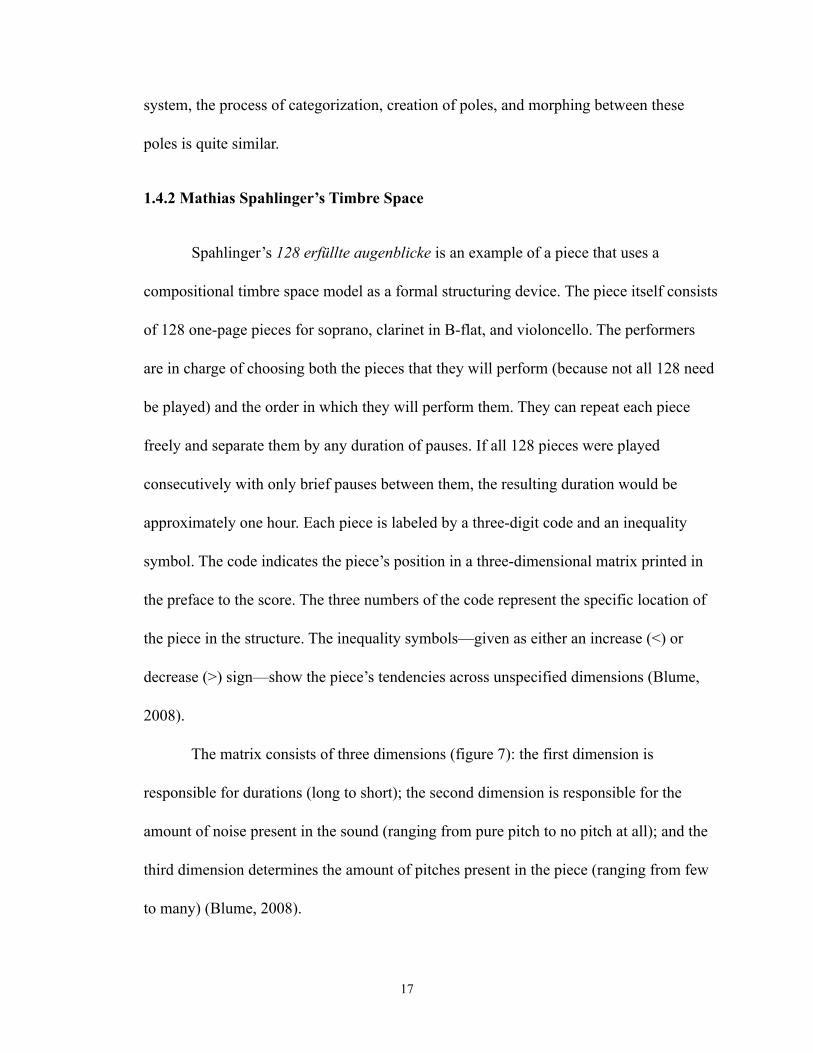
The matrix consists of three dimensions (figure 7): the first dimension is

responsible for durations (long to short); the second dimension is responsible for the

amount of noise present in the sound (ranging from pure pitch to no pitch at all); and the

third dimension determines the amount of pitches present in the piece (ranging from few

to many) (Blume, 2008).

17

The matrix configuration is theoretically set up to allow the listener to be able to

tell where the individual piece is within the space. This interpretation is aided by the

division of each dimension into four units. Each unit (labeled 1-4 in its slot), controls a

distribution of identifiable extremes. For example, in the duration axis, the scale ranges

from longer to shorter. Instead of breaking this down into extremely short, short, medium,

and long, the units each contain a range of events. For example, in the type n2n (the 2

refers to the second unit along the duration axis) long values dominate the majority of the

sounds. In contrast, n3n has more short than long values (Blume, 2008).

In the case of the pitch to noise dimension (the third digit), nn1 indicates that the

sounds are pitched; nn2 denotes that there are mostly pitched sounds with a few noisy

ones; nn3 signifies that the piece consists of mostly noisy sounds with some clear pitches;

and nn4 is essentially noise (Blume 2008).

18

Figure 7. Timbre space from Spahlinger’s 128 erfüllte augenblicke. As adapted from the preliminary remark to 128 erfüllte augenblicke, by M. Spahlinger, 1975.

In the “different pitches” axis (indicated by the first digit), 1nn means that all the

sounds have the same pitch; 2nn means that the majority of the pitches are repeated; 3nn

means that pitches rarely repeat themselves; and 4nn means that no pitch is repeated

(Blume, 2008).

While the dimensions and units of the piece seem fairly straightforward, the

inequality symbols are a little more vague. Each piece appears to represent a motion

relative to its position in an unspecified direction which either gradually increases or

decreases along individual axes in terms of its rate of pitch repetitions, noise factor, or

shortness/longness of notes. These transitional factors can combine with one another or

cross paths. In essence, the inequality signs suggest movement within each piece (Blume,

2008).

I find this timbral model interesting because it sets up identifiable coordinates for

the listener. In my own pieces, I similarly use categories that explore noise and the

amount of material present at any one time.

1.4.3 Kaija Saariaho’s “Timbral Axis”

Saariaho’s work approaches timbre from many different angles. I have been

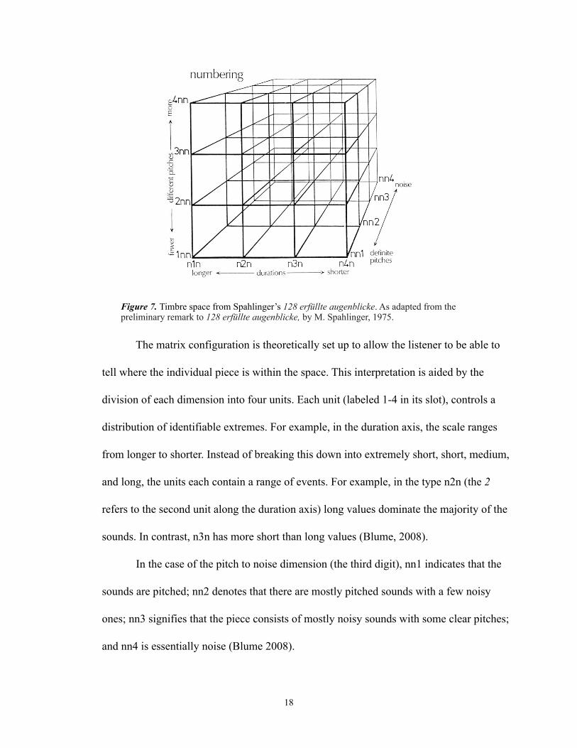
intrigued by both her works and her “timbral axis” (illustrated in figure 8). Using this

axis, Saariaho formally controls the timbral organization of her compositions. Similar to

both Penderecki’s and Spahlingers’ spaces, Saariaho sets up a system that allows for clear

timbral poles. These poles create a sense of tension and relaxation in her music and could

be described as sine waves versus white noise, or clear versus noisy sounds. In her article

“Timbre and harmony: interpolations of timbral structures” Saariaho pondered: “along

19

this axis, generally speaking, ‘noise’ replaces the concept of dissonance and ‘sound’ that

of consonance” (Saariaho, 1987, p.93). Saariaho uses this axis to develop both musical

phrases and larger forms which she believes creates inner tension in her works.

Saariaho often speaks of how she perceives timbre and harmony as separate entities,

timbre being a vertical process and harmony a horizontal one. She thinks that “harmony...

provides the impetus for movement, whilst timbre constitutes the matter which follows

this movement. On the other hand, when timbre is used to create musical form it is

precisely the timbre which takes the place of harmony as the progressive element in

music” (Saariaho, 1987, p.94). These two elements can become confused when timbre

becomes an integral part of form and when harmony is confined to determining the

general sonority. As with many spectral and post-spectral composers, timbre and

harmony end up as indistinguishable through the morphology of the sounds. Saariaho’s

sound axis is reminiscent of the system used by Grisey which controls the harmonic

progression from harmonicity to inharmonicity, as well as the temporal progression from

order to disorder (Rose, 1996). The concept of the “timbral axis” was important in

Saariaho’s first major orchestral work, Verblendungen, which was composed at IRCAM,

and can also be seen in her piece Jardin secret I.

20

Figure 8. Saariaho’s “timbral axis.” Adapted from “The Works of Kaija Saariaho, Philippe Hurel and Marc-André Dalbavie—Stile Concertato, Stile Concitato, Stile Rappresentativo,” by S. Pousset, 2000, Contemporary Music Review, 19(3), p. 83.

Saariaho’s timbral axis has been very influential in my works, and I have based a

few of my compositions on it, including my piece Sparrow (Spero). Also, in my most

recent timbre model, my noise dimension behaves very similarly to Saariaho’s “timbral

axis.”

1.5 Timbre Models in My Music

While I have been attracted to timbre models conceived by other composers and

researchers, I have sought a model for my purposes that is less limited and open to deeper

dimensionality. Saariaho questioned the mono-dimensionality of her axis. She pondered,

“...I wonder if there might be ways to organize timbre in more complex—hierarchical?—

ways” (Saariaho, 1987, p.93). The goal for creating my own compositional timbre model

was to find a way to allow the perceptual properties of timbre to address and control any

aspect of a composition across multiple dimensions.

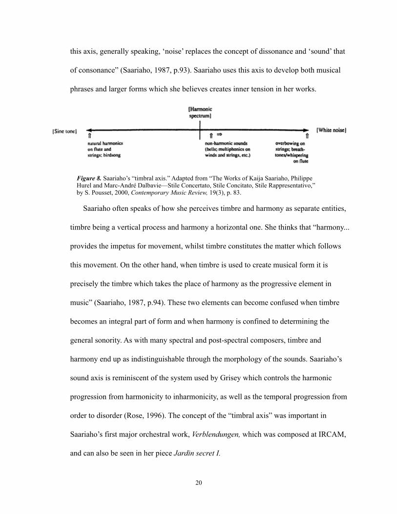
For my own works I propose a set of two interlocking spaces or “cubes” as I like

to call them. Diagrams of the timbre spaces can be seen in figure 9.

The first cube essentially controls the frequency components of the sound. This

compositional timbre space has the following three dimensions: spectral flux, spectral

centroid, and noise-to-pitch ratio. The first dimension, spectral flux, measures the

Euclidean distance between two spectra, or rather, the change of spectral energy over

time. By extension, this dimension can be used to control rhythms or the frequency of

pitch changes. This analogy provides a measure of density in time analogous to spectral

flux at the intra-event level. For example, in my model, a sound with high flux means that

there is a high rhythmic activity, or that pitches are changing quickly, while a sound with

21

low flux would be one in which there is either a low rhythmic activity, or the pitches are

stagnant.

The second dimension controls the noise-to-pitch ratio and is similar to Saariaho’s

“timbral axis.” On one end of the axis there are sounds that are mostly “pure” pitch—that

is, sounds that are close to sine waves. By contrast, the other end of the axis is “mostly

noise.”

The third dimension controls the spectral centroid, or rather, the average centroid

over time, and controls the brightness and darkness of the sound. For example, if the

space was evaluating the spectral centroid for a violin sound, this axis would have four

reference points—con sordino, sul tasto, normale, and sul ponticello—plus every shifting

possibility in between.

22

Figure 9. Timbre spaces used in my own works

In this model, each dimension changes depending on the source material inserted

into it and the function of the desired result. To illustrate I will briefly examine some of

the compositional possibilities of the noise-to-pitch axis. This dimension could be used to

control the bow and finger pressure of a string player (pure sounds being harmonics and

noisy sounds being increased bow pressure), or it could be used as a filtering device for

material (a single filtered frequency on the “mostly pitch” end and the maximum number

of desired frequencies on the “mostly noise” end). One could also use this model to learn

more about a sound’s timbral characteristics, or one could map a composition’s

instrumentation onto the space, thereby creating spatial coordinates for every sound they

wish to use and “seeing” the possible relationships among them. Using this model timbre

itself can be used to control and inform a composition. It can be used to derive rhythms,

generate a form, harmony, and rate of material, or simply inform the orchestration of the

piece. With this model one can work with any sound or instrumentation. While this

process is far more intuitive than scientific, it abstracts the original sound and allows one

to base a piece’s timbral decisions upon an already existing acoustic model.

Cube I is, however, missing key information, namely: the quality of the attack, the

dynamic level, and the length of the event entering into the space. To solve this dilemma I

use a secondary cube to inform these decisions. This second cube works in conjunction

with cube I. The first dimension—attack—controls how the sound or gesture’s

articulations are treated, ranging from no attack (or a smooth onset) to a sharp attack

(sharp onset); the second dimension controls the length of the event, sound, or gesture

that enters into the timbre cube; and the third dimension controls the dynamics. Virtually

23

any aspect of a composition can be viewed and decisions can be made based on these two

combined cubes.

This space was used in three of my most recent pieces: Ostiatim, Clocca, and

Occupied Spaces.

II. Ostiatim (2011)

2.1 Introduction

Through a series of fifteen fragments, Ostiatim explores the sounds produced by

doors and the emotional inflections of the people who interact with them. The title,

meaning “door-to-door,” is meant to depict the timeline of the piece. Each fragment

should be treated like a fleeting memory. Sometimes connections are made, and other

times the moment slips away.

The composition was inspired by the sculpture Memory by Anish Kapoor. I saw

the work at the Guggenheim Museum in 2010. The sculpture plays with one’s memory by

giving the viewer limited access points from which to view it. The majority of the

sculpture is hidden from view, and the observer is charged with mentally placing the

pieces of the puzzle—what the entirety looks like—together.

The sculpture inspired Ostiatim in many ways. Firstly, the title of the sculpture,

Memory, influenced the fragment form of the piece and the long pauses often found

between fragments. Secondly, the overall number of fragments (fifteen) was based on the

ribbing from a particular angle of the sculpture. From this view (seen in figure 10), the

sculpture has fifteen sections that all meet and touch at both an inner and outer circle.

Finally, the source materials for the piece, door sounds, were chosen because they

24

reminded me of both the passageways that one had to walk through, and the window that

one had to look into in order to view the sculpture. Similarly for me, the shapes formed

by the sculpture’s ribbing were reminiscent of doors. Ostiatim takes these shapes and

translates them into doors, or rather uses them as catalysts for exploring the emotions of

the people who interact with them.

I began work on the piece by recording a variety of door sounds. I was amazed to

find that specific emotions can be inferred based on how one opens, closes, or knocks on

a door.3 While the sound of doors is common in electronic music my goal was to

acoustically orchestrate these doors and abstract them, teasing out gestures and melodies

25

3 I became intrigued by the idea after examining the research done by Stanford student Laurel Anderson on the possible emotional inflections of door sounds. The research paper was completed for the class “Psychophysics and Cognitive Psychology for Musicians,” taught by Jonathan Berger at Stanford University.

Figure 10. Anish Kapoor’s Memory. Adapted from The Deutsche Bank Series at the Guggenheim Anish Kapoor Memory,” by D. Heald, Retreived May 31, 2013, from http://web.guggenheim.org/exhibitions/kapoor/index2.html. Copyright 2008 by The Solomon R. Guggenheim Foundation.

in the process and allowing the listener to hear the same sounds with different musical

intentions.

The six sounds used in this piece are: doorchimes, westminster doorchimes, a

door banging, a door slamming, knocking, and a door creaking. For each sound, I made

dozens of analyses, both of the sound’s original form, and of compressed and expanded

temporal forms. Then I chose a certain number of these analyses and built a program in

OpenMusic4 to help me study them more carefully. I quantized the frequency analyses

into chromatic semitones and then chose between one and three versions of each of these

sounds. Finally, I arranged them into fifteen fragments.

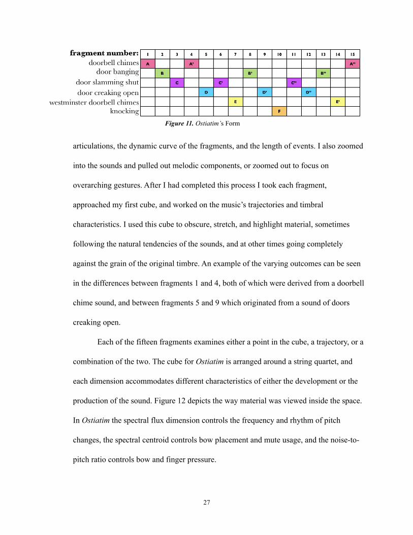
2.2 Form

The fifteen fragments of the piece were arranged according to a set of simple pre-

defined rules: no two pairs of sounds could repeat in the same order twice over the course

of the piece5 and the sounds were meant to be gradually introduced over time. The form

for the source materials in Ostiatim can be seen in figure 11.

2.3 Timbre as a Morphing Device

In this piece timbre was largely treated as a morphing device. After determining

the overall form of the piece I began to massage the analyses of the sounds and form

material. The first pass at the piece was composed with cube II in mind. I focused on

26

4 OpenMusic (OM) is a visual programming language based on Common Lisp. The program is a particularly useful environment for music composition. OM was designed by the IRCAM Music Representation research group.

5 For example, if the sound doorbell chimes (listed as A) and door banging sounds (listed as B) were played in succession, the AB pattern could not occur again over the course of the piece.

articulations, the dynamic curve of the fragments, and the length of events. I also zoomed

into the sounds and pulled out melodic components, or zoomed out to focus on

overarching gestures. After I had completed this process I took each fragment,

approached my first cube, and worked on the music’s trajectories and timbral

characteristics. I used this cube to obscure, stretch, and highlight material, sometimes

following the natural tendencies of the sounds, and at other times going completely

against the grain of the original timbre. An example of the varying outcomes can be seen

in the differences between fragments 1 and 4, both of which were derived from a doorbell

chime sound, and between fragments 5 and 9 which originated from a sound of doors

creaking open.

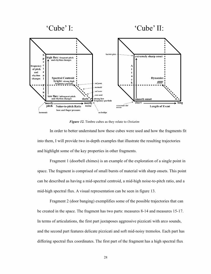
Each of the fifteen fragments examines either a point in the cube, a trajectory, or a

combination of the two. The cube for Ostiatim is arranged around a string quartet, and

each dimension accommodates different characteristics of either the development or the

production of the sound. Figure 12 depicts the way material was viewed inside the space.

In Ostiatim the spectral flux dimension controls the frequency and rhythm of pitch

changes, the spectral centroid controls bow placement and mute usage, and the noise-to-

pitch ratio controls bow and finger pressure.

27

Figure 11. Ostiatim’s Form

In order to better understand how these cubes were used and how the fragments fit

into them, I will provide two in-depth examples that illustrate the resulting trajectories

and highlight some of the key properties in other fragments.

Fragment 1 (doorbell chimes) is an example of the exploration of a single point in

space. The fragment is comprised of small bursts of material with sharp onsets. This point

can be described as having a mid-spectral centroid, a mid-high noise-to-pitch ratio, and a

mid-high spectral flux. A visual representation can be seen in figure 13.

Fragment 2 (door banging) exemplifies some of the possible trajectories that can

be created in the space. The fragment has two parts: measures 8-14 and measures 15-17.

In terms of articulations, the first part juxtaposes aggressive pizzicati with arco sounds,

and the second part features delicate pizzicati and soft mid-noisy tremolos. Each part has

differing spectral flux coordinates. The first part of the fragment has a high spectral flux

28

Figure 12. Timbre cubes as they relate to Ostiatim

while the second part has a mid-low flux. The spectral centroid has multiple trajectories.

One can observe the motion in the second violin and the violoncello. For example, in

measure 8 they move from sul ponticello to ordinario which can be viewed as a

movement from a high to a mid spectral centroid. Another example can be seen in

measure 12 with a movement back to sul ponticello. Here, the spectral centroid shifts

back to high. In measure 13 they shift to sul tasto which can be viewed as a movement to

a low spectral centroid. The violoncello then does one more movement to sul ponticello,

and then plays ordinario in measures 13-15 which can be viewed as the trajectory of a

high to low spectral centroid.

In terms of the noise-to-pitch axis, in measure 8 both the second violin and the

violoncello move from over-pressured bowing to normale bowing. This can be viewed on

the timbre cube as a movement from a high noise-to-pitch ratio to a mid-low one. The

opposite motion can be seen again in measures 11-12 and 13-14. Furthermore, in the

second part of this fragment (measures 15-17) the second violin and viola explore a mid-

29

Figure 13. Ostiatim’s Fragment 1—points in space for cubes 1 and 2

high noise-to-pitch ratio while the first violin (mm.15-17) and the second violin (mm.17)

explore a mid-noise coordinate. A visual representation of these trajectories can be seen

in figure 14.

While I will not go into detail on every fragment, I will point out some highlights:

fragment 5 (door creaking open) primarily explores the noise-to-pitch axis through finger

pressure; fragment 6 primarily has to do with the mode of attack, dynamics, and length of

events; and fragment 7’s primary motion is one from a high spectral flux in measures

47-50 to a low spectral flux in measures 51-53.

There are also overarching timbral poles and trajectories occurring in the piece.

For example, the “brightest” fragment is number 12 while the “darkest” one is fragment

14. Also, the noisiest fragment is number 10 while the “purest” one is fragment 14.

The finished composition is a series of abstracted door sounds that explore both

the gritty noisy aspects of these sounds and the beautiful “emotional” side of them. The

30

Figure 14. Ostiatim’s Fragment 2—trajectories in space for cubes 1 and 2

finished product is not meant to be a replica of the original but rather an interpretation of

it.

With this piece I was working with a type of musique concrète instrumentale. The

term was coined by composer Helmut Lachenmann. In essence, musique concrète

instrumentale honors the original sound sources by observing what happened within the

sounds. Here is an example given by Lachenmann himself: “If I hear two cars crashing—

each against the other—I hear maybe some rhythms or some frequencies, but I do not say

‘Oh, what interesting sounds!’ I say, ‘What happened?’ The aspect of observing an

acoustic event from the perspective of ‘What happened?’, this is what I call musique

concrète instrumentale” (Steenhuisen, 2004, p.10).

III. Clocca

3.1 Introduction

The next piece in my portfolio is titled Clocca, and is for chamber ensemble.

Clocca is a piece that explores sounds associated with time. The latin title, meaning

“bell,” is a precursor to the English word “clock,” and is meant to illustrate the intrinsic

connection between time, clocks, and bells.

The piece was written as a response to Sparrow (spero), for flute, violin, horn,

piano, percussion, and live-electronics, which I wrote in 2008 at McGill University.

While both pieces have entirely different focal points, they are both structured around the

same bell sound. This bell resides in a historical meeting house in my home town of

Jaffrey, NH. Similar to many New England towns, this bell sounds every hour. While it is

31

one of the sounds of my childhood, the bell’s location and history are also important. It is

housed in a meeting house that was erected on June 17, 1775 during the battle of Bunker

Hill. Tradition tells us that the workers could hear the sounds of cannon fire from

Charlestown. The bell tower was added in 1822 and the bell was cast by the Paul Revere

Foundry (Stephenson & Seiberling, 1994). The form for Clocca is based on the structure

of this bell sound.

3.2 Form: Timbre as a Structuring Device

! I began this piece by analyzing the bell’s spectrum and spectral flux. I reduced the

bell sound to its 37 most salient partials and analyzed their decay. An analysis that

illustrates the 37 partials and their cut-offs can be seen in figure 15.

The overarching form of the piece is a retrograde of the bell sound followed by

an original bell sound. I used the bell’s individual partials as structuring mechanisms.

Other bell sounds commonly associated with time and bells were also inserted between

32

Figure 15. Analysis of Clocca’s bell sound illustrating 37 paritals and their cut-offs

the structural partials as blocks of material. For the retrograde of the bell sound I

calculated the timings of each partial and then multiplied them by a factor of seven.6 A

diagram that lists the partial numbers and the approximation of their cut-offs in seconds

can be seen in figure 16.

33

6 The number seven was chosen because it best represented the proportions I had envisioned for the piece.

Figure 16. Partial numbers and cutoff times for the bell sound

In the piece, each partial is presented in retrograde as it would appear in the bell

sound. For example, the partial that lasts the longest, number 37, has a frequency of 236

and lasts 38.2 seconds. In the piece itself this is the first presented partial and was

structured to enter 4 minutes and 27.4 seconds before the climax. As the bell gets closer

to its attack, the introduction rate of partials increase. The piece ends with an “original”

38-second version of the bell, played forward and in “real time.” For each retrograde bell

partial entrance I generated a series of spectra that moved from the original bell’s

spectrum to an increasingly distorted spectrum. The fundamental frequency of each

spectrum gradually shifts down. The original bell’s partials function as center frequencies

in the distorted spectrum and were part of the process that derived the new spectra. In the

piece itself each original partial is played as a held note while the new spectral

components are articulated through sweeping upward or downward gestures. The gradual

distortion of the spectra and original entrance partials can be seen in figure 17.

While the original bell does provide the overall vertical structuring points for the

piece, other material associated with time and bells is used as well. These are inserted

between structural moments. The first partial of the piece is not even presented until

approximately two minutes into the piece and simply appears to blend into the

background. The piece begins with large blocks of materials derived from other bell and

clock sounds. Examples of these other sounds are: alarm clocks, kitchen timers, chimes,

school bells, domestic clocks, fire alarms, wind chimes, and some more abstract

representations of sounds such as crickets and dripping water.

34

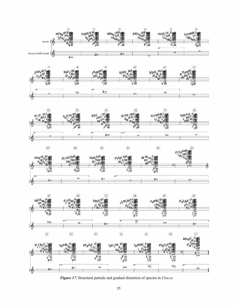
35

Figure 17. Structural partials and gradual distortion of spectra in Clocca

The blocks gradually become shorter and shorter as the piece progresses and more

bell partials are introduced. The partials become so frequent as they near the bell’s attack

that they completely overtake the material. As previously mentioned, the piece ends with

a single iteration of the overarching bell sound. This “coda” of sorts is the first time the

listener hears all of the bell’s partials together.

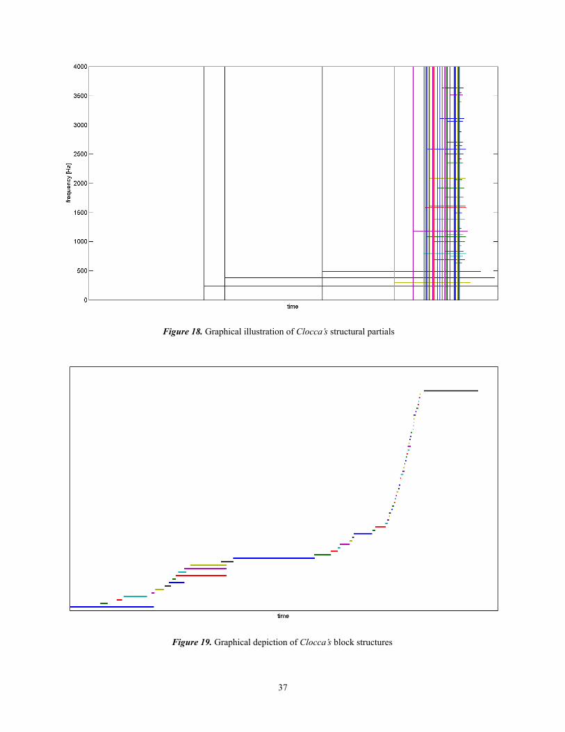
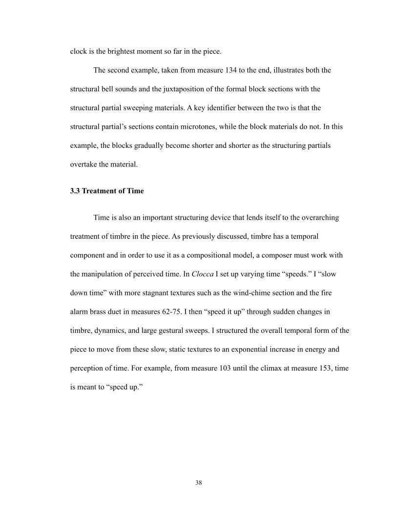
Figures 18 and 19 are graphical representations of the form that help illustrate the

processes occurring in Clocca. Figure 18’s vertical lines depict the piece’s structural

partials and their beginning and end points. The horizontal lines illustrate the 37 entrance

points. Figure 19 visually depicts the blocks of material over time.

In terms of the piece’s timbral trajectory, the two iterations of the bell sound

(elongated retrograde and original) provide the large-scale trajectory of the piece, while

the individual blocks provide separate small-scale ones. To illustrate I will discuss two

examples. The first example illustrates the small-scale trajectories and occurs from

measures 1-59, and the second occurs from measure 134 to the end.

At the beginning of the piece, I began with a sparse, dry, and percussive timbre.

The source material is dripping water, a reference to the modern clock’s water clock

origin. The piece begins with percussive woodwind and wooden percussion drips, and

gradually increases in density, activity, and noise. The strings enter with a subtle

introduction of select bands of the original bell sound and then add to the dripping texture

before gesturally sweeping upwards. This section is followed by the piano playing

“clock” material. It begins with regular, metrical “ticks” that gradually become sporadic

and are interrupted by a shocking, bright, and metallic “alarm clock” sound. This alarm

36

37

Figure 18. Graphical illustration of Clocca’s structural partials

Figure 19. Graphical depiction of Clocca’s block structures

clock is the brightest moment so far in the piece.

The second example, taken from measure 134 to the end, illustrates both the

structural bell sounds and the juxtaposition of the formal block sections with the

structural partial sweeping materials. A key identifier between the two is that the

structural partial’s sections contain microtones, while the block materials do not. In this

example, the blocks gradually become shorter and shorter as the structuring partials

overtake the material.

3.3 Treatment of Time

Time is also an important structuring device that lends itself to the overarching

treatment of timbre in the piece. As previously discussed, timbre has a temporal

component and in order to use it as a compositional model, a composer must work with

the manipulation of perceived time. In Clocca I set up varying time “speeds.” I “slow

down time” with more stagnant textures such as the wind-chime section and the fire

alarm brass duet in measures 62-75. I then “speed it up” through sudden changes in

timbre, dynamics, and large gestural sweeps. I structured the overall temporal form of the

piece to move from these slow, static textures to an exponential increase in energy and

perception of time. For example, from measure 103 until the climax at measure 153, time

is meant to “speed up.”

38

IV. Occupied Spaces

4.1 Introduction

The third piece presented in this portfolio is Occupied Spaces, a work for two

pianos and percussion. It was premiered by the ensemble Yarn/Wire. The idea for the

piece originated through the concept of timbre in space and the topic of Normalized Echo

Density (NED). NED describes how the reflections of a sound in a given space interact

over time, and the texture that results. Some of the key terms and components associated

with NED are: the sound’s clarity, focus and blur, the perception of smoothness and

roughness or rather the degree of granularity of the sound, the ratio of direct to reflected

signal in the sound, the dryness or wetness of a signal, and the description of the number

of reflections per second of an acoustic signal. For example, noises with low NED would

be perceived as “sputtery” and noises with high NED, would be perceived as

“smooth” (Huang, Abel, Terasawa & Berger, 2008).

Occupied spaces is a piece that explores timbre through a series of eleven

“rooms” or conceptual spaces. Some of these spaces have been modeled after physically

existing rooms, others are either imagined (and do not follow the rules of physics), or

occur inside one’s mind/head.7 There are three impulses in the piece: a zipper, a clap, and

a balloon pop. These impulses form the material that is inserted into the various rooms.

The sounds are filtered to various degrees, and over the course of the piece frequencies

39

7 The room that occurs “inside” the listener’s mind/head includes two categories. The first is a figurative and imagined space that is devoid of walls and quite literally can be thought of as the listener imagining material. The “physical” space is the listener’s skull cavity. This “space” somewhat changes in dimensions as the piece progresses and is (clearly) imagined.

are added to the impulses, thereby creating an increasingly dense—and by analogy—

noisy texture.8 For example, in measure 7 near the beginning of the piece, only a single

frequency is present within the room. By contrast, over 43 partials are present during the

climax in measure 289. The full spectrum of the clap can be seen in measure 288.

Similarly, the full spectrum of the balloon pop can be seen in measure 289. The zipper is

treated gesturally and is often marked through steady sweeps upwards and/or accelerating

tremolos in tam-tams, gongs, or other metallic percussion. Specific “zipper” pitches can

be periodically heard, for example in measures 34, 71, 110, 135, 139, 156, 166, and 174.

4.2 Form

The piece’s overall form is divided into an introduction and six main sections.

Each section determines which rooms are presented, how many rooms can be present at

any one time, and the degree of the noise-to-pitch ratio. Also, in each section impulses

have been organized into various strands of material. Each strand comes from a two-part

theme that is presented in the first section. Each section takes this theme and

destructively varies it. The original theme can be seen in figure 20. This first iteration can

be found in measures 7-33. As one can see, part A of the theme is comprised of balloon

material, and part B of clap material.

The piece begins with an introduction of the zipper in room 19 that hints at some

of the characteristics of the rooms, followed by section 1 that introduces rooms 2-4 and

40

8 While the densification of frequencies in itself does not equate with an increased level of noisiness, in the case of Occupied Spaces, the impulses themselves are different noises. Therefore, as more frequencies are added, by analogy, the true “noisy” nature of the sound is revealed, thus creating an increasingly noisy texture.

9 In Occupied Spaces, the zipper always occurs in room 1.

the two basic strands of thematic material. Section 2 introduces rooms 5 and 6 and the

strands begin to grow and overlap. Section 3 presents rooms 7 and 10 and the possibility

of three simultaneous strings and two overlapping rooms. Section 4 introduces room 8

and strings begin to multiply and deteriorate the “structure” of all the rooms.10 The zipper

attempts to overwhelm the material but it is repeatedly interrupted and cut off by room 8.

Section 5 begins after a final failed attempt by the zipper and the first iteration of room 9.

The balloon and clap theme begins section 6 and tentatively attempts to reset the rooms,

however, they have deteriorated and reflections begin to multiply. The strands proliferate

while the reflections increase in density until they have completely saturated all of the

rooms. A final iteration of the clap, balloon, and zipper form the climax of the piece.

Section 6 is marked by the second iteration of room 9, which takes the third climactic

impulse (the zipper, which finally succeeds in overwhelming the material) and leads the

listener into the final new room: number 11. This last room reminiscently employs a

41

10 The deterioration is accomplished through a combination of the rooms misbehaving and by an uncontrollable increase in the number of reflections and echoes. As the rooms begin to increasingly overlap and thematic strands of material begin to multiply, the rooms begin losing or exchanging some of their characteristic components, thereby dissolving into the listener’s imagination (room 1).

Figure 20. Example of Occupied Spaces two-part theme

small bandwidth of frequencies from the previously heard impulses, creating a ghost-like

resonance. The piece closes with a brief recap and final presentation of fragments of the

original theme and a brief presentation of select rooms. A visual representation of the

overarching formal structure of the piece can be seen in figure 21 and a graph that

illustrates the individual timings of the rooms can be seen in figure 22.11

42

11 Figures 21 and 22 illustrate different aspects of the form. The timings for figure 21 were taken from the premiere performance, whereas the timings for figure 22 were taken directly from the score. Slight differences are the consequence of performance liberties. Figure 22 depicts the room start and stop times. Please note: after section 4, the rooms have deteriorated to a point that many are unrecognizable. For the purpose of the graph they have been listed as room 1, however, they stem from other spaces.

Figure 21. Spectrogram and graphical representation of Occupied Spaces’ form

Figure 22. Graphical illustration of the temporal room spatialization

As previously mentioned, each section controls the noise-to-pitch ratio present at

any given time. Each section ranges from having one to multiple noise trajectories and

strands of thematic material. Similarly, the overall piece moves from small bands of

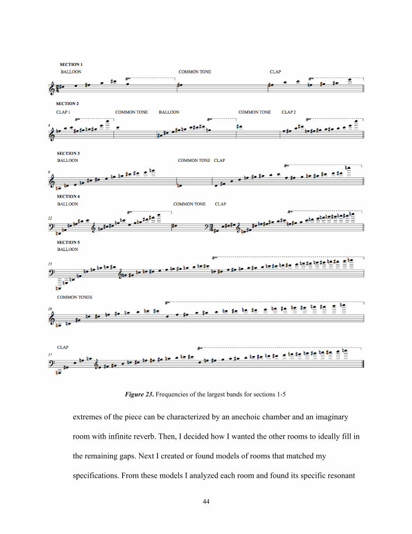
filtered material to the sound’s “full spectrum12.” Figure 23 illustrates the frequencies of

the largest band in the first five sections. It is worth noting that, between the clap and the

balloon, in sections 1-4 there is only one common pitch present at any given time. In

section 5 there are many common pitches present. As previously mentioned, the rooms

have deteriorated and there are so many layered strands of material that both the balloon

and clap pitches become nearly indistinguishable.

4.3 Eleven Rooms: Timbre in Space

Now that the treatment of the zipper, clap, and balloon material has been

discussed, it is important to understand how the rooms themselves work, and how they

interact with the inserted sounds.

When creating the form of the piece I decided there would be eleven individual

rooms. In my research, I looked at different impulse responses in various rooms, analyzed

reverbs, created delay patterns, and considered the resonant properties of different spaces.

Similar to the NED properties already discussed, I came up with room classifications that

were based on the following specifications: how dry/wet the sound is, how many

reflections there are, the degree of granularity, the characteristics of the overall sound,

and how resonant the space is. I wanted to make sure I covered a broad range of room

possibilities so I first determined what the extremes of the rooms would be. The two

43

12 The “full” spectrum is taken to be all spectral components retained after initial filtering and reduction.

extremes of the piece can be characterized by an anechoic chamber and an imaginary

room with infinite reverb. Then, I decided how I wanted the other rooms to ideally fill in

the remaining gaps. Next I created or found models of rooms that matched my

specifications. From these models I analyzed each room and found its specific resonant

44

Figure 23. Frequencies of the largest bands for sections 1-5

properties, determined the exact rhythm of the reflections (if there were any), and

analyzed the room’s dynamic curve. Then, I inserted the impulses themselves into each

room and analyzed the results. I carried out this process with both the original noise

impulses and with a single pitch—B4. The resulting analyses can be seen in figure 24.

After completing this process I orchestrated the results, choosing the instruments that best

followed the room’s characteristic properties. The rooms themselves are described below,

and the resulting orchestration can be viewed in figure 25.

Room 1 first appears in the introduction from measures 1-6. As previously

described, this room is imaginary and “places” the impulse material inside the listener’s

head/mind. In essence, the material is either left untouched (if it is inside the listener’s

mind), or has a slight echo (it if is inside the listener’s head) and is devoid of any further

manipulation. The impulse can be played by any instrument; however, the piano most

commonly plays this material.

Room 2 is first introduced in measure 7. This room is the driest of all the (actual)

rooms and has no reflections or added resonance. The room is essentially an anechoic

chamber. The inserted material remains very short with no sustain. In this space the

impulse is colored by what would be the naturally occurring harmonic series for the given

pitches. These harmonics are always three dynamic levels lower than the impulse

material. For example, if the impulse is f, then the emphasized harmonics would be p.

The impulse and the room can be played solo by either piano 1 or 2, or in combination by

both pianos.

45

46

{{

{{

pp

1 2

f f

f mf mf mp

3 4

3

pp ppp f mf

°f mf mp mf p

°

5 6

5

mp f p pp ppp

° ø f mp mf p

°

mp f ppp

7

7

f ppp

°

24

24

&

Instrumentation: anyFirst appearance: mm. 1-7

!

Instrumentation: pianos 1 & 2 First appearance: mm. 7 ”“Æ

Original Analyses

& Æ

&

Instrumentation: xylophone & marimbaFirst appearance: mm. 10

*Æ> -”“ Instrumentation: toy piano, piano 2, cow bell, suspended cymbal and marimba

First appearance: mm. 15”“

&

*The xylophone and marimba natrually sustain the material. Regardless of whatis written in the score, the result will remain constant.

Æ ->

*These pitches are a resonant characteristic of the room. Depending on the impulse material the upper notes may change. The A3 will remain constant.

*

&

Instrumentation: piano (either 1 or 2), wind chimes, crotales and vibraphoneFirst appearance: mm. 39

Instrumentation: piano 1, celesta and triangleFirst appearance: mm. 56

> > >”“

3

& >>

3

&

Instrumentation: celesta, vibraphone, glockenspiel, crotalesFirst appearance: mm. 73 (beat 5) - 75”“

3

&

œœœœœœ###

"

œ " œ "

œœœœœœ###R

œœœœœœ ™™™™™™ œœœœœ#

##" Œ

" œ " Œ

œR œ ™ ˙" "œœœ#nn

" Œ

œœœœ

#

#

œœœœ##

# œ œ œ ‰ Œ Ó !œœœœœ### ™™™™™

œ œ œ œ œ œ œ œ " ™

œœ ™™™™ œœ ™™ œœ œœ œœ ™™ œœ œ ™ w œ ™ Ù ‰ œ ‰ œœœœœ# œœœœ œ œ œ œ "

œœœœ## œœœœ# œœœ

" ™œœœœ " ™

œ œ œ œ œ œ œ œœ œÙ ® " Ù

œ ™ œ ™ œ œ ™ œ œ œ œ ™ œŒ

œ ™ œ œ œ ™ œ ™ œ œ ™ œ œ œ œ œ ™ œ ™ œ œ ™ œ œ œ œ ™ œ Œ

Figure 24 (Part I). Original analyses of rooms on the pitch B4

47

Figure 24 (Part II). Original analyses of rooms on the pitch B4

48

{

{

{

{

{

°

¢{°

¢{

{

1 2 3 4

Triangle

Wind Chimes

Cymbal

Wood Block

Bass Drum

Crotales

Tubular Bells

Marimba

CymbalCowbell

GongTam-tam

Timpani

Glockenspiel

Xylophone

Vibraphone

Piano I

Toy Piano

Piano II

Celesta

1414141414

14

14

14

14

141414

14

14

14

14

14

14

14

14

14

2424242424

24

24

24

24

242424

24

24

24

24

24

24

24

24

24

8484848484

84

84

84

84

848484

84

84

84

84

84

84

84

84

84

/First appearance: mm. 1

!First appearance: mm. 7

! ! ! ! !First appearance: mm. 10

!First appearance: mm. 15

!/ ! ! ! ! ! ! ! !/ ! ! ! ! ! ! ! !/ ! ! ! ! ! ! ! !/ ! ! ! ! ! ! ! !

& ! ! ! ! ! ! ! !

& ! ! ! ! ! ! ! !

& ! ! ! ! ! ! impulse

pp ppp

reflection 1Æ -mf

reflection 1

/ ! ! ! ! ! ! !mp p

/ ! ! ! ! ! ! ! !? ! ! ! ! ! ! ! !

& ! ! ! ! ! ! ! !

& ! ! ! ! ! !

emphasis of harmonics in room

f mf

Æ> -!

& ! ! ! ! ! ! ! !

&

can appear in any instrument

!

room: slight emphasis of harmonics

pp

!pp

room: slight emphasis of harmonics

Æ”“! ! ! !

Æ

&impulse

f

impulse

f

! ! ! impulse

f

Æ ! !Æ

& ! ! ! ! ! ! ! impulse

f

>

& !pp

room: slight emphasis of harmonics

! !pp

room: slight emphasis of harmonics

Æ!

Æreflection 1

mp

”“

& ! impulse

f

impulse

f

Æ ! ! !mf

room: emphasis of harmonics

Æ”“

& ! ! ! ! ! ! ! !

? ! ! ! ! ! ! ! !

œR œ ™ " " œœœ#nn " Œ

œ œ ‰ Œ

œœœœœœ###R

œœœœœœ ™™™™™™

"

œœœœœœ###

‰™œœœœœœ###

‰™

œ ‰™ œ ‰™ œ ‰™

˙

Œœœœœœœ###

‰™œœœœœœ###

‰™ "œ

" Œ

Œ œ ‰™ œ ‰™ œœœœœ###

Œ

Figure 25 (Part I). Orchestration of rooms

49

{

{

{

{

{

°

¢{°

¢{

{

5

9

6

Tri.

W.Ch.

Cym.

W.B.

B. D.

Crot.

Tub. B.

Mar.

Cym.Cow.B.

Gong

Timp.

Glock.

Xyl.

Vib.

Pno. I

T. Pno.

Pno. II

Cel.

°

° ø °

°

8484848484

84

84

84

84

8484

84

84

84

84

84

84

84

84

84

84

2424242424

24

24

24

24

2424

24

24

24

24

24

24

24

24

24

24

7474747474

74

74

74

74

7474

74

74

74

74

74

74

74

74

74

74

/First appearance: mm. 15

Úmf

First appearance: mm. 56

mp

>pp

/mp

sputtery nature of the room

!

/ Ú !/ Ú !/ Ú

sputter - emphasizing a harmonic of the impulse

!

&mf

resonance of the room

mp

!

& Ú !

& Ú !

/ Ú !

/ Ú !? Ú !

& Ú !

& Ú !

&mf

sputter - resonance of the room

emphasizing a harmonic of the impulse

!

&mp

impulse + room emphasis of harmonic

f

reflection 1reflection 2

p

reflection 3

pp

reflection 4

ppp f

impulse

reflection 2

mp

reflection 3 + room emphasis of harmonics

mf

>> reflection 4

reflection 5reflection 6

p

reflection 7

3

& Ú !

& Ú !

&the material in piano 1 above can also be played by piano 2 as need be Ú !

& Ú !

& Úroom emphasis of harmonics

f mf

reflection 1

mp

reflection 2

*

* on occasion, this is absent

mf

reflection 3> > >reflection 4

reflection 5

p

reflection 6

3

? Ú !

œ ™ œ ® œ " ‰

œ ‰ Œ Ó !

" œ œ œ ‰ Œ Ó !

œœ#œ ‰™ Œ Ó !

œœ ™™™™ œœ ™™ œœ œœ œœ ™™ œœ œ ™ w œ ™ Ù ‰ œ ‰ œœœœœ# œœœœ œ œ œ œ "

œœœœœ### ™™™™™

œ œ œ œ œ œ œ œ " ™

Figure 25 (Part II). Orchestration of rooms

50

{

{

{{

{

°

¢{

°

¢

{

{

711

8

Tri.

W.Ch.

Cym.

W.B.

B. D.

Crot.

Tub. B.

Mar.

Cym.Cow.B.

Gong

Timp.

Glock.

Xyl.

Vib.

Pno. I

T. Pno.

Pno. II

Cel.

°

°

°

°

747474747474

74

74

7474

74

74

74

74

74

74

74

74

74

74

74

181818181818

18

18

1818

18

18

18

18

18

18

18

18

18

18

18

585858585858

58

58

5858

58

58

58

58

58

58

58

58

58

58

58

404404404404404404

404

404

404404

404

404

404

404

404

404

404

404

404

404

404

/First appearance: mm. 73 (beat 5) - 75

!First appearance: mm. 136-137

! !/ ! ! !/ ! ! !/ ! ! !/ ! ! !

&ppp

room - sputtery harmonics

ppp

! !

& ! ! !

& !room

f

>

p ff

/ ! ! !

/ ! ! !

? !

* from the highest to lowest possible pitch

f

*>

p

reflections

ff

>

&mp

*room - sputtery harmonics

f ppp

! !3

& ! ! !

&

* not all of these pitches are played. Material is taken from these figures

mp

reflection 2* reflection 3

reflection 4reflection 5

p

(room harmonics)

p

(echo)

pppp

! !

& !

impulse

f

>

p

harmonics emphasized by the room

˙̇#ff

& ! ? room

>‘“& ?

& ! ! !

& ! !

harmonics emphasized by the room

f

”“> >

& ! !>

?

&f mf p ppp

! !

?impulse reflection 1 reflection 6 reflection 7 reflection 8

! !

Œ Œ ‰™ Ù œ# ™ œ ™ œ œ ™ œ œ œ œ ™ œ Œ

œ#J æææœn æææœ æææœ# æææœ ™ æææœn æææœ æææœ ‰

1J æææ æææ ææææææ- -

œœœœ##

œœœœ# œœœ " ™ œœœœ " ™ œ œ œ œ œ œ œ œœ œ Ù ® ‰ !

Œ " ™ œ ™ œ œ ™ œ œ œ# ™™™ Œ Œ " ® œ ™ œ œ ™ œ Ù œ# ™™™

œJ˙̇b

‰

œœœœœ#n j ‰

œœœœ## œœœœ## ™™™™

‰ ‰ Œœœœœ# ™™™™ ‰ Œ

Œ Œ ‰™ Ùœ# ™ œ ™ œ œ ™ œ œ œ œ ™ œ

Œ

œ ™ œ œ œ œ ™ œ œ ™ œ ™ œ œ ™ œ œ œ œ ™ œ Œ

Figure 25 (Part III). Orchestration of rooms

51

{

{{

{{

°

¢

{°

¢{

{

914

Tri.

W.Ch.

Cym.

W.B.

B. D.

Crot.

Tub. B.

Mar.

Cym.Cow.B.

Gong

Timp.

Glock.

Xyl.

Vib.

Pno. I

T. Pno.

Pno. II

Cel.

404404404404404404

404

404

404404

404

404

404

404

404

404

404

404

404

404404

545454545454

54

54

5454

54

54

54

54

54

54

54

54

54

5454

/ !First appearance: mm. 177-181

/ !/

fff

room

>

/ !/

fff

room

>p o

& !

&reflection 1*

f* The placement of this pitch varies

& !

/ !

/ !

? !

& !

& !

&

room resonance / reflections

MOTOR ON

* pitches and rhythms were selected from here

mp

*

pp

°

&fffff

impulse>*

?

* pitches and rhythms were selected from here

room resonance / reflections

p

*

pp ppp°

& !

&fffff

impulse>

?p

room resonance / reflections

* pitches and rhythms were selected from here

*

*

pp ppp°&

& !? !

œ Œ Œ Ó™ Ó™ Ó™ Ó™ Ó™ Ó™ Ó™ Ó™ Ó™ Ó ! !

œ Œ Ó æææ̇ æææw æææw ™ æææw æææw ™ æææw æææw æææw æææ̇

‰ œ Œ Œ Ó™ Ó™ Ó™ Ó™ Ó™ Ó™ Ó™ Ó™ Ó™ Ó ! !

Ó˙̇̇̇̇̇̇̇̇̇̇˙̇̇̇̇˙̇̇

###

n#n##n#nn##nn#

˙̇̇̇̇˙̇̇̇̇˙̇nnn

™™™™™™™™™™™™ ˙̇̇

˙̇̇̇̇˙

œœœœœœœœœ ™™™™™™™™™

œœœœœœœ#n ™™™™™

™™wwwwwww

œœœœœœœ

™™™™™™™ œœœ

jwww ™™™ ˙̇̇ œœœ

j˙ œ ™ w ™ ˙ œj œ ™

w Œ Œ Ó™ Ó™ Ó™ Ó™ Ó™ Ó™ Ó™ Ó™ Ó ! !

Ó

˙̇̇̇̇̇̇˙̇̇̇̇̇̇̇̇̇˙̇̇̇̇̇˙̇̇˙

#

n##n#n###n####nnn#n##n ˙̇̇̇̇

˙̇̇̇̇̇˙̇̇̇˙

nn#n

™™™™™™™™™™™™™™™™ ˙̇̇

˙̇̇̇̇˙̇̇˙n

n

Œ Ó ! ! ! ! ! ! !

w Œ Œ Ó™ Ó™ Ó™ Ó™ Ó™ Ó™ Ó™ Ó™ Ó ! !

Ó

˙̇̇̇̇̇̇˙̇̇̇̇̇̇̇̇̇˙̇̇̇̇̇˙̇̇˙

#

n##n#n###n####nnn#n##n ˙̇̇̇̇

˙̇̇̇̇̇˙̇̇̇˙

nn#n

™™™™™™™™™™™™™™™™ ˙̇̇

˙̇̇̇̇˙̇̇˙n

n

Œ Ó ! ! ! ! ! ! !

Figure 25 (Part IV). Orchestration of rooms

52

{

{

{

{

{

°

¢

{°

¢

{

{

1015

11

Tri.

W.Ch.

Cym.

W.B.

B. D.

Crot.

Tub. B.

Mar.

Cym.Cow.B.

Gong

Timp.

Glock.

Xyl.

Vib.

Pno. I

T. Pno.

Pno. II

Cel.

545454545454

54

54

545454

54

54

54

54

54

54

54

54

54

54

444444444444

44

44

444444

44

44

44

44

44

44

44

44

44

44

/First appearance: mm. 90-94

! !First appearance: mm. 296-300

/ ! !/ ! !

/ ! !/ ! !& ! !

& ! !

&p

reflectionsthese begin steady and become erratic

pp

. . . . . . . . . etc.

o!

. .

/ ! !

/ ! !? ! !

& ! !

&these begin steady and become erraticreflections

pp ppp

. . . . . . .etc.

o!. .

&

MOTOR OFFroom resonance

!

°

&f

impulse

mf

reflectionsthese begin steady and become erratic- . . . . . . .

o.

impulse e-bowU

? ! !

& ! !

&mf

echo

mp

reflectionsthese begin steady and become erratic- . . . . . etc.

o

. . . room 11 can be played by both pianos 1 and 2.

!

& ! !

& ! !

? ! !

Œ ‰™ œ# œ œ# œ œ# œ œ œ# œ œb œb‰

Œ Œ " œ# œ œ# œ œ# œn œn œ# œn ‰

˙̇̇̇n# ™™™™ Ó

œ œ œ# œ œ# œ œ œ# œ ‰™ Ó w

" " œ œ œ# œ œ# œ œ œ# œ " Œ Œ

Figure 25 (Part V). Orchestration of rooms

Room 3 first appears in measure 10 and is the brightest of all the rooms. This

room alters the perception of the original impulse. The overall effect of this room is an

EQed sound that is extremely dry and bright. The room has one reflection and a short

reverb of approximately two seconds. The reflection always occurs one sixteenth-note

after the impulse and is slightly sustained. Similar to Room 2, the impulse’s natural

harmonics are present; however, in Room 3 the harmonics are emphasized and

overshadow the original impulse. In the dynamic curve of the room, the harmonics are

always three dynamic levels higher than the impulse material and the reflection is one

dynamic level lower than the impulse. For example, if the impulse is p, then the

emphasized harmonics (or rather the resonance of the room) would be f. For this room

the impulse is articulated by the marimba and the room/harmonics are played by the

xylophone.

Room 4 is introduced in measure 15 and has a slight reverb of just under 1.4

seconds, a high resonant factor, and one audible reflection. The room distorts the sound

of the impulse by adding inharmonic components and adds both a high resonance that

occurs with the attack of the sound and a low addition tone that occurs with the

reflection.

In this room the impulse is played by the toy piano which is naturally inharmonic.

The resonance of the room is emphasized by piano 2 and the suspended cymbal which is

played simultaneously by the toy piano at one to two dynamic levels lower than the

impulse. The piano plays one dynamic level lower than the toy piano and the cymbal

plays two levels lower. The reflection is played by the marimba, piano 2, and the cow

53

bell, and occurs one sixteenth-note after the impulse. The marimba and cow bell represent

the room’s resonance.The marimba always plays an A4 and one to three additional

pitches from the room’s natural resonance. This reflection is one dynamic level lower

than the original impulse. The piano’s reflection is a high harmonic of the original

impulse and is two dynamic levels lower than the original impulse.

The first instance of Room 5 occurs in measure 39. Room 5 has a moderate reverb

and an overall sound that is slightly sputtery. There are four clear reflections following

the impulse. The room emphasizes the first natural harmonic (an octave higher) of both

the impulse and three of the following reflections. The reflections have the following

dynamic curve: two dynamic levels higher, one lower, two lower, and then three lower

than the initial impulse. For example, if the impulse was mp, the reflections would be f,

p, pp, and ppp, respectfully.

Overall, the room has a “shimmery” quality, which is reflected by the

orchestration. The granularity of the impulse is orchestrated via a sweep of the wind

chimes that coincide with two 32nd notes played by the vibraphone, followed by two

64th notes and one 32nd note in the crotales. The room’s natural resonance is played by

both the vibraphone and the crotales. The vibraphone plays an A#3 and C4, and the

crotales play a G6 and C6. After playing the room’s resonant pitches, the vibraphone and

crotales emphasize harmonics from the impulse.

Room 6 first appears in measure 56. This room has seven reflections and an

approximate reverb time of 3.6 seconds. The overall sound of the room is highly

resonant, bright, and metallic. Piano 1 plays the initial impulse plus six reflections.

54

During the third reflection the piano also highlights some of the sound’s upper harmonics.

In the orchestration the celesta acts as the part of the room that emphasizes the impulse’s

harmonics which it cycles through with each reflection. The triangle both colors the

impulse and highlights individual reflections. The dynamic characteristics of the room

follow the subsequent sequence: impulse; followed by the first reflection which is one

dynamic level lower than the impulse; reflection 2 which is two dynamic levels lower;

reflection 3 that features a slight surge in the signal and is only one dynamic level; and

reflections 4, 5, 6, and 7 which naturally fade to three dynamic levels lower than the

original impulse.

Room 7 is not heard until measure 73 (beat 5) and persists to measure 75. Room 7

is highly reflective, has a moderate reverb, and an overall sputtery sound. The room has a

high resonance and is the most “metallic” of all the rooms. The impulse has eight clear

reflections that gradually fade. The room highlights the impulse’s upper harmonics and

causes a kind of swirl pattern that slowly dissipates. The impulse and initial attack is

highly colored by harmonics.

In this room the impulse is played by the celesta. The vibraphone and the celesta

play the subsequent reflections. The glockenspiel, crotales, and the celesta play the

sputtery metallic harmonics that are emphasized in the room.

Room 8 is first introduced in measures 136-137. This room is very dry and has a

maximum number of reflections. It is an “imagined” space and reflections increase in

intensity as time passes—something that would not naturally occur in a real room. In my

55

original analyses 33 clear reflections could be identified. However, due to the speed of

the reflections I simplified them into a multi instrument tremolo.

The instruments used to orchestrate this room are marimba, timpani, piano 1, and

piano 2. The marimba plays a figure (common in both the original analyses and the

orchestration), and represents part of the natural resonance of the room. The timpani

plays the reflections of the impulse. Piano 1’s left hand plays the impulse, while the right

hand plays the dark and gritty resonance of the room, followed by harmonics of the

impulse (mixed with room’s resonance) as a tremolo. Piano 2 plays harmonics of the

original impulse.

Room 9 only appears twice throughout the piece. It first appears from measures

177-181. Room 9 is the most reverberant of all the rooms. It is also highly reflective and

sputtery. The reverb tail is approximately 20-25 seconds. The resulting resonance of the

room seems to pulse and is dark and low in pitch.

The room was orchestrated using pianos 1 and 2 as the impulse, and the bass

drum and vibraphone as the resonance and reflections of the room. The vibraphone’s

motor is on for this section and provides a pulsing sensation. The tubular bells articulate a

single clear reflection and the cymbal and bass drum color the impulse, helping

orchestrate the gritty nature of the room.

Room 10 first appears in measures 90-94. The room is very dry and has many

clear reflections. This room is somewhat odd because it starts with the impulse and then

articulates a repetitive strand of sporadic and sputtery sixteenth-note reflections that step

upwards chromatically. The impulse and the strand are echoed as well. This echo begins

56

on the third sixteenth-note of the original strand. The room itself has a resonance that

presents itself with the initial impulse.

For orchestration, room 10 uses both pianos, the marimba, xylophone, and

vibraphone. The impulse, first strand, and echo begin in pianos 1 and 2. Strand one then

moves to the marimba while strand two moves to the xylophone. The overall effect is that

the sounds are thinning out and becoming dryer and brighter. The room’s resonance is

played by the vibraphone. In the original analysis the resonance is quite dense and

gradually steps upwards with the reflections. I simplified this in the piece and the

vibraphone plays a single four-note sustained chord.

The eleventh and final room of the piece represents an imaginary space that has a

smooth onset and an infinite sustain. There are no reflections in this space, simply an

“infinite reverb.” This sound is achieved by the pianists playing e-bows on the piano

strings and occasional bowed vibraphone sounds. Room 11 first appears in measures

296-300 and is the last new room presented.

In Occupied Spaces the impulses interact with the rooms. Both are essentially

convolved. The rooms morph the inserted material and provide their own timbral

trajectories. The finished piece is the result of the collision of two formal elements: the

rooms themselves and the material inserted into them.

V. Summary and Conclusions

My primary objective as a composer is to write beautiful and stimulating music.

For me, “beauty” is embodied by temporal, and in particular, timbral attributes. Over the

past five years I have been working towards a compositional model in which the “color”

57

and “texture” of available sounds are derived from models of timbre spaces.

While I have been attracted to other composers’ and researchers’ timbre models

(including Penderecki, Spahlinger, Saariaho, Grisey, Slawson, Lerdahl, Cogan, and

Erickson, to name just a few), I found them too limited in their scope and therefore

strived to create one that combined many models into one. In my own research I have

pored over the literature, studied perceptual timbre models, and picked a few studies,

including Pollard and Janson’s tristimulus model, Wessel’s timbre model, Grey’s timbre

space, McAdams’ timbre space, and the vocal tract filter, and tried to imagine how these

studies could inform a composition. While this exercise was useful and suggests ways for

a composer to manipulate musical parameters, they are missing a key element: no

unpitched percussion or noise elements are explained. In order to encompass this crucial

dimension I proposed a set of two spaces. The first space covers the frequency

components of the sound and has the following dimensions: spectral flux, spectral

centroid, and noise-to-pitch ratio. The second space controls the evolution of the sound

and controls the attack quality, event duration, and the dynamic curve for any entering

sound, gesture, or material. With this model, one can work with any sound or

instrumentation. While this process is intuitive, it allows one to base a piece’s timbral

decisions on an already existing acoustic model.

In my most recent works I have used nature sounds as stimuli and “everyday”

sounds as material for my pieces. I am fascinated by the “color” of sounds and timing of

events that surround us in our everyday lives. They are filled with rich material and offer

incredible musical possibilities. With my model one can insert material into the space and

58

zoom in and out of it as one desires. Similar to painting, with this model the composer

not only gets to choose the “landscape,” the composer can also control the perception and

magnification of the material. The dimensions change slightly depending on what one

chooses to highlight. Similar to visual art, the resulting piece would not be a copy of the

source, but rather a representation of it.

The three pieces that form my final project examine both the compositional

application of timbre spaces and the exploration of the concept “timbre in space.” Each

piece approaches timbre from a different perspective. Ostiatim explores the orchestration

of noise and the use of timbre as a morphing device. Timbre informs the overarching

formal structure as well as the material in Clocca; and Occupied Spaces explores timbre

in space through filtered impulses and a series of rooms or spaces.

With each piece I compose I understand more, not only about timbre and the

different ways to approach my composition model, but also about time and space. With

this model each composition serves as a piece of a puzzle whose image reveals a more

clear and complete understanding of not only timbre, but all musical parameters.

VI. Scores

6.1 Score for Ostiatim

The score for Ostiatim appears on pages 60-70.

59

60

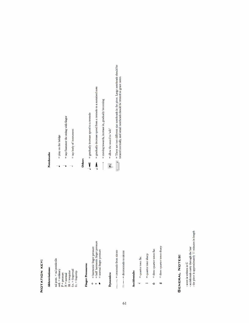
61

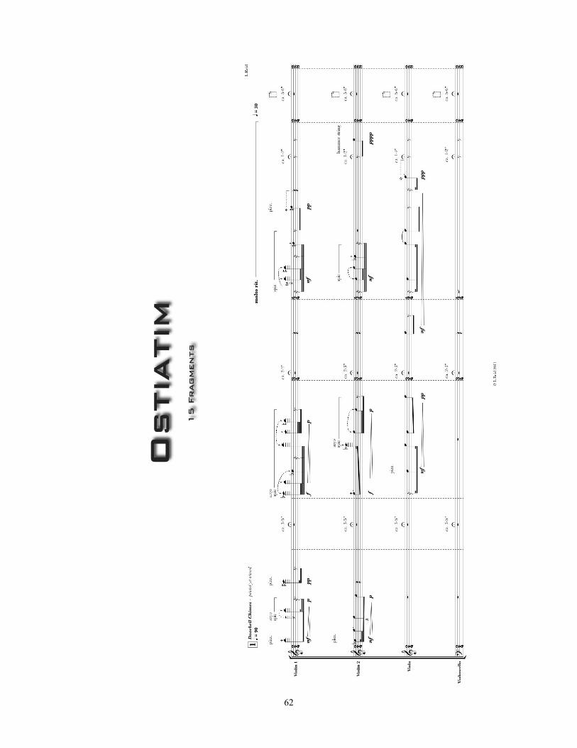
62

63

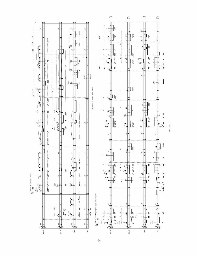
64

65

66

67

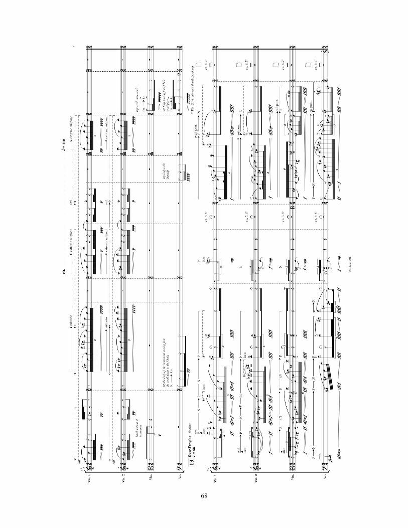
68

69

70

6.2 Score for Clocca

The score for Clocca appears on pages 72-105.

71

72

73

74

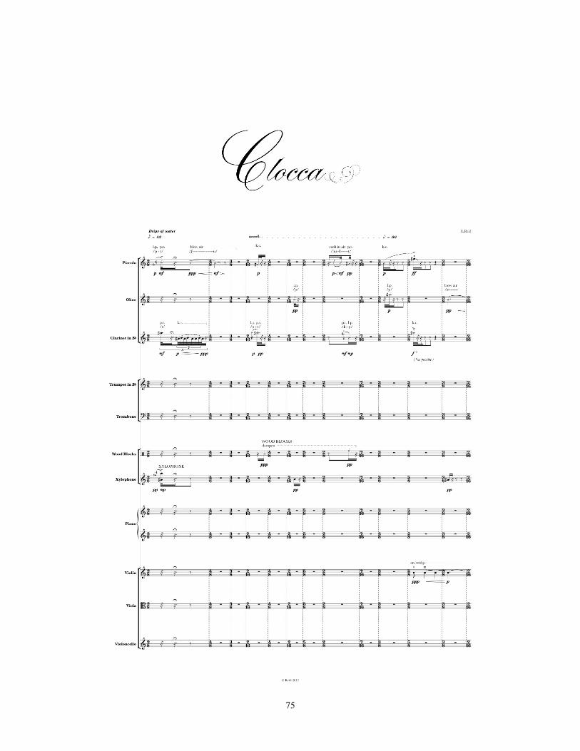
75

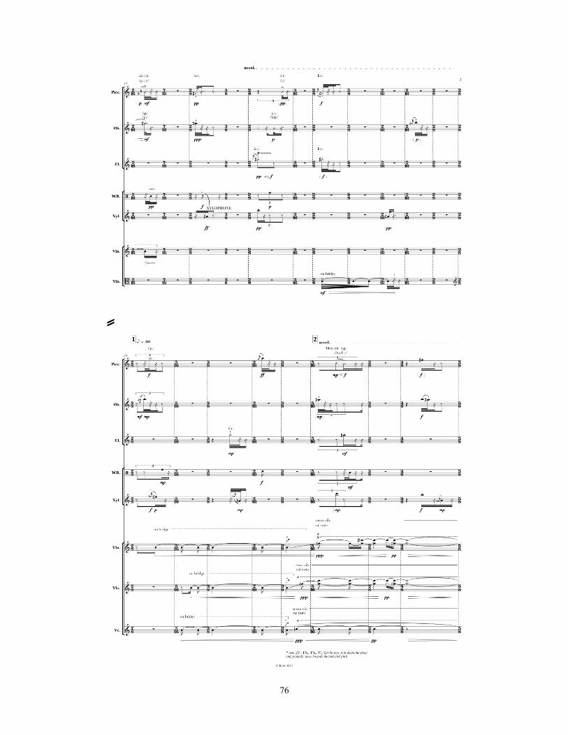
76

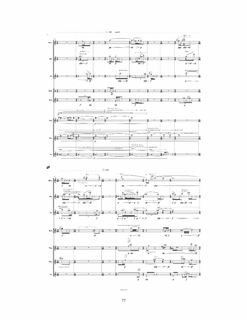
77

78

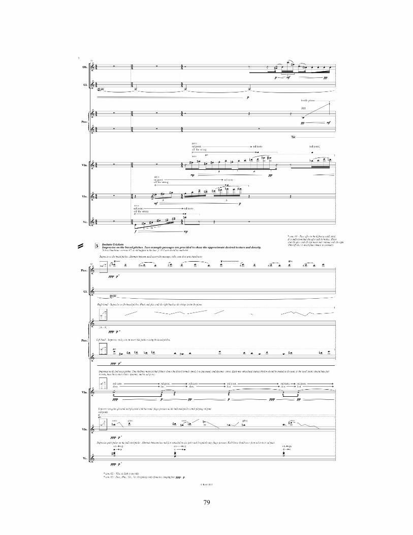
79

80

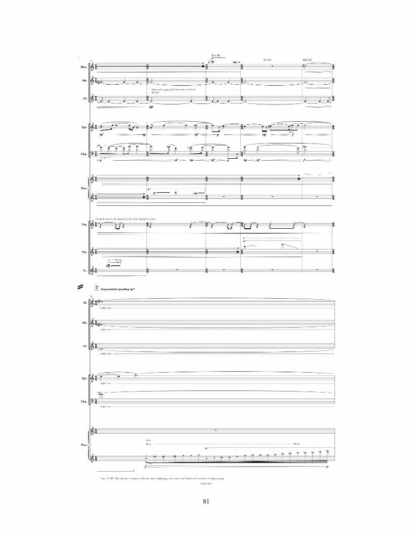
81

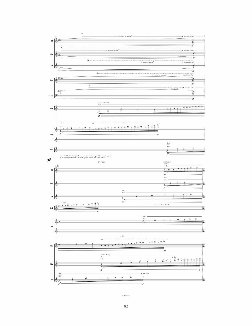
82

83

84

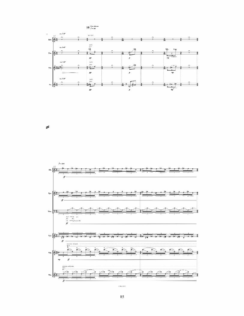
85

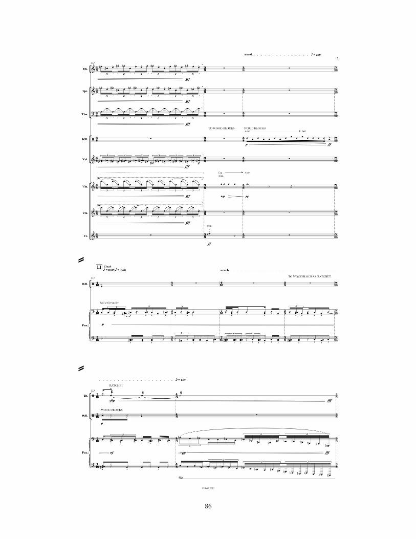
86

87

88

89

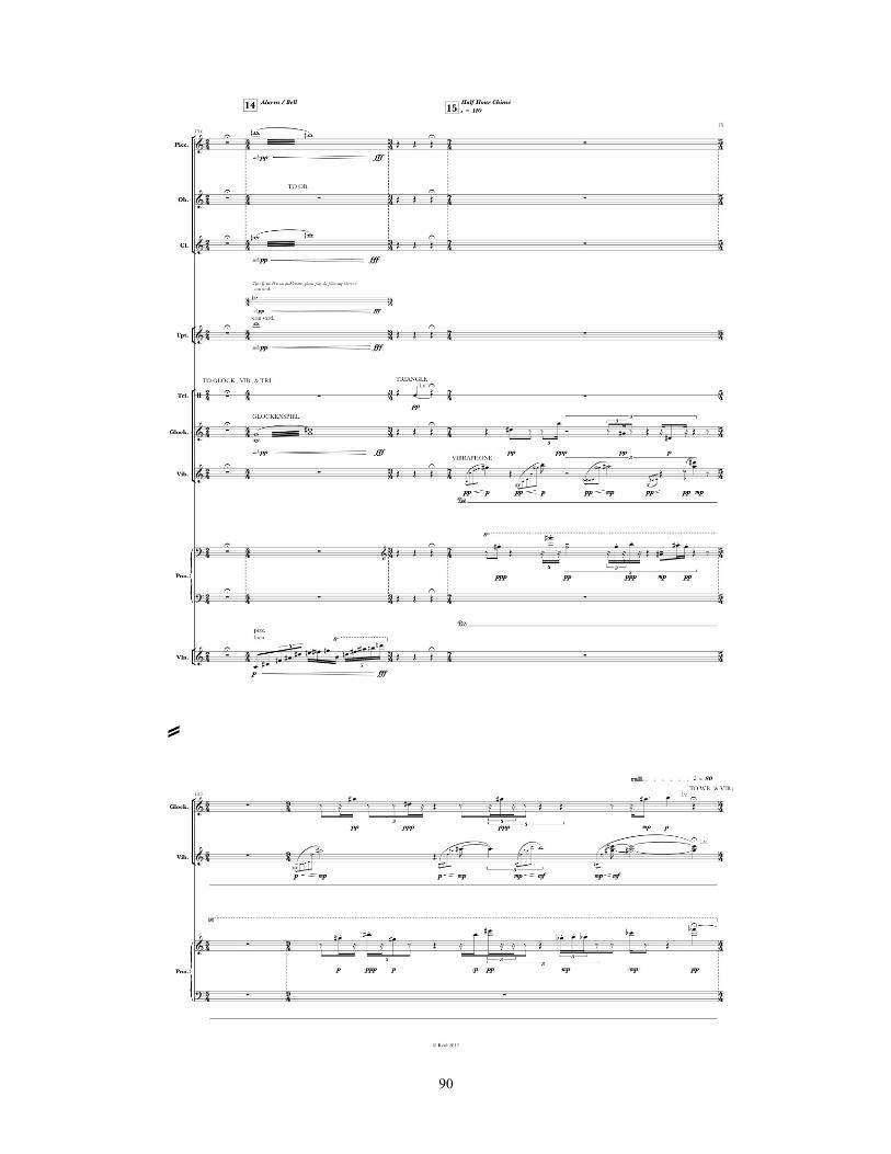
90

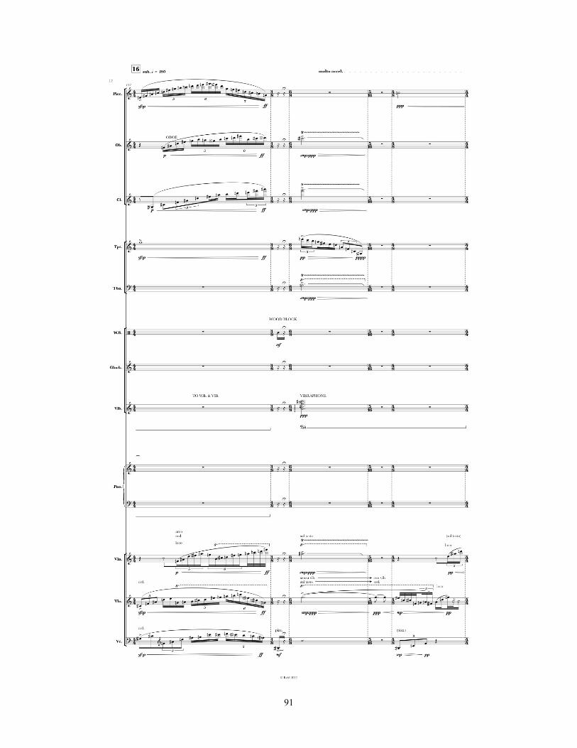
91

92

93

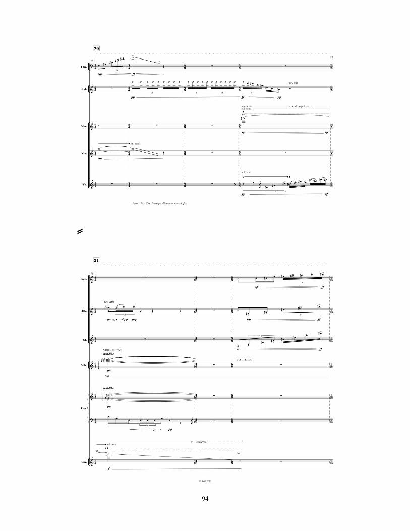
94

95

96

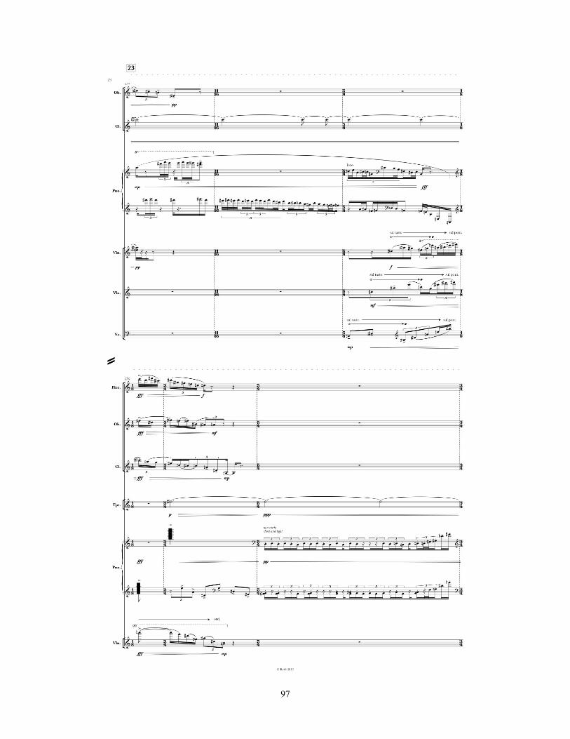
97

98

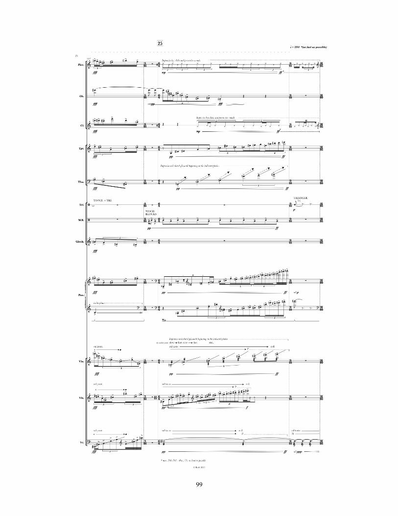
99

100

101

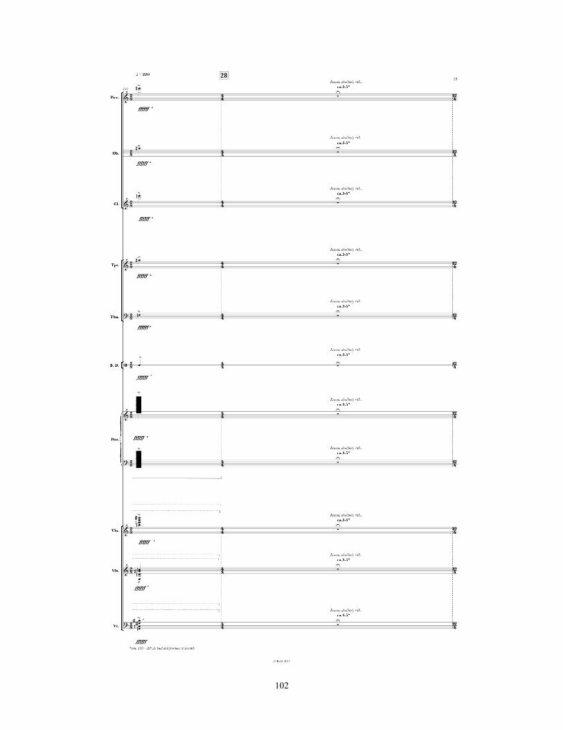
102

103

104

105

6.3 Score for Occupied Spaces

The score for Occupied Spaces appears on pages 107-153.

106

107

108

109

110

111

112

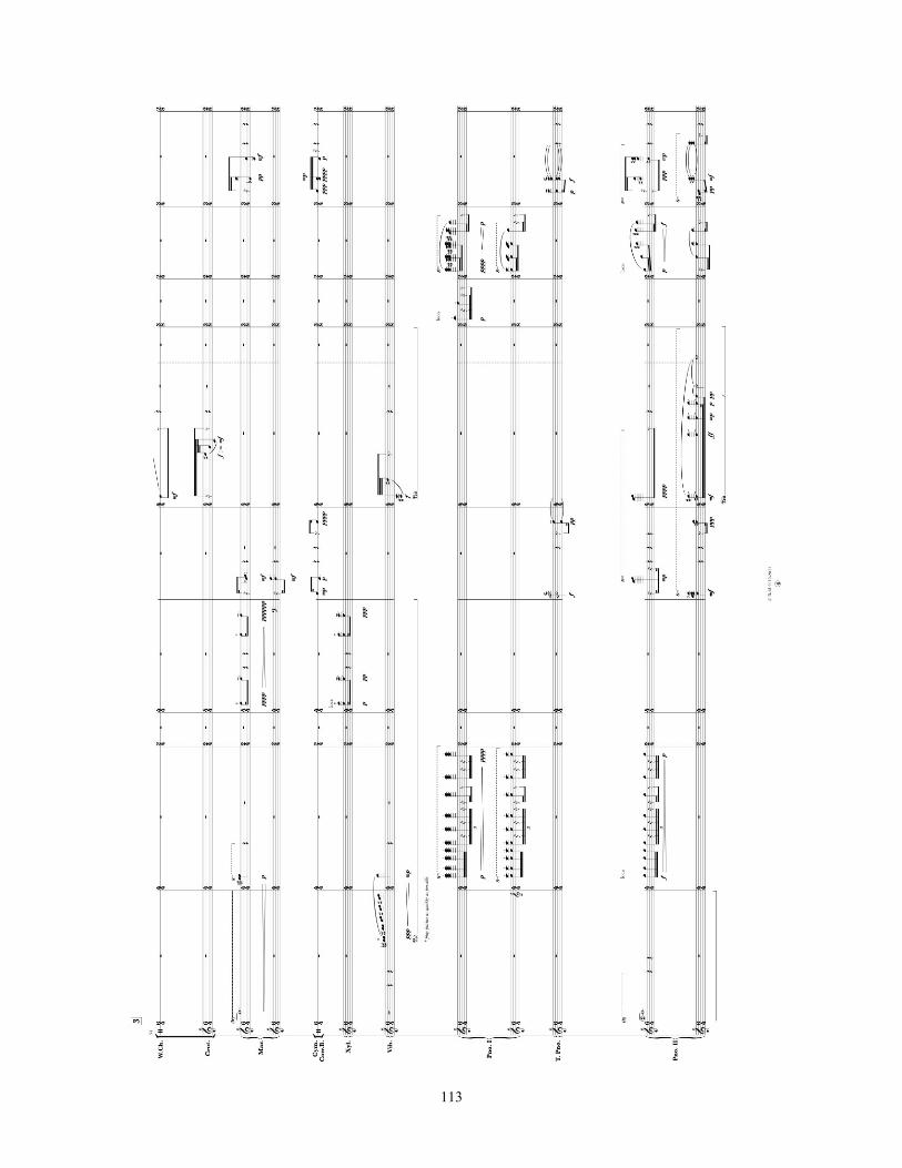
113

114

115

116

117

118

119

120

121

122

123

124

125

126

127

128

129

130

131

132

133

134

135

136

137

138

139

140

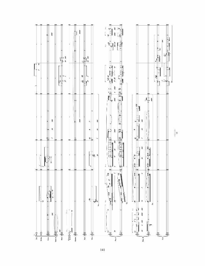
141

142

143

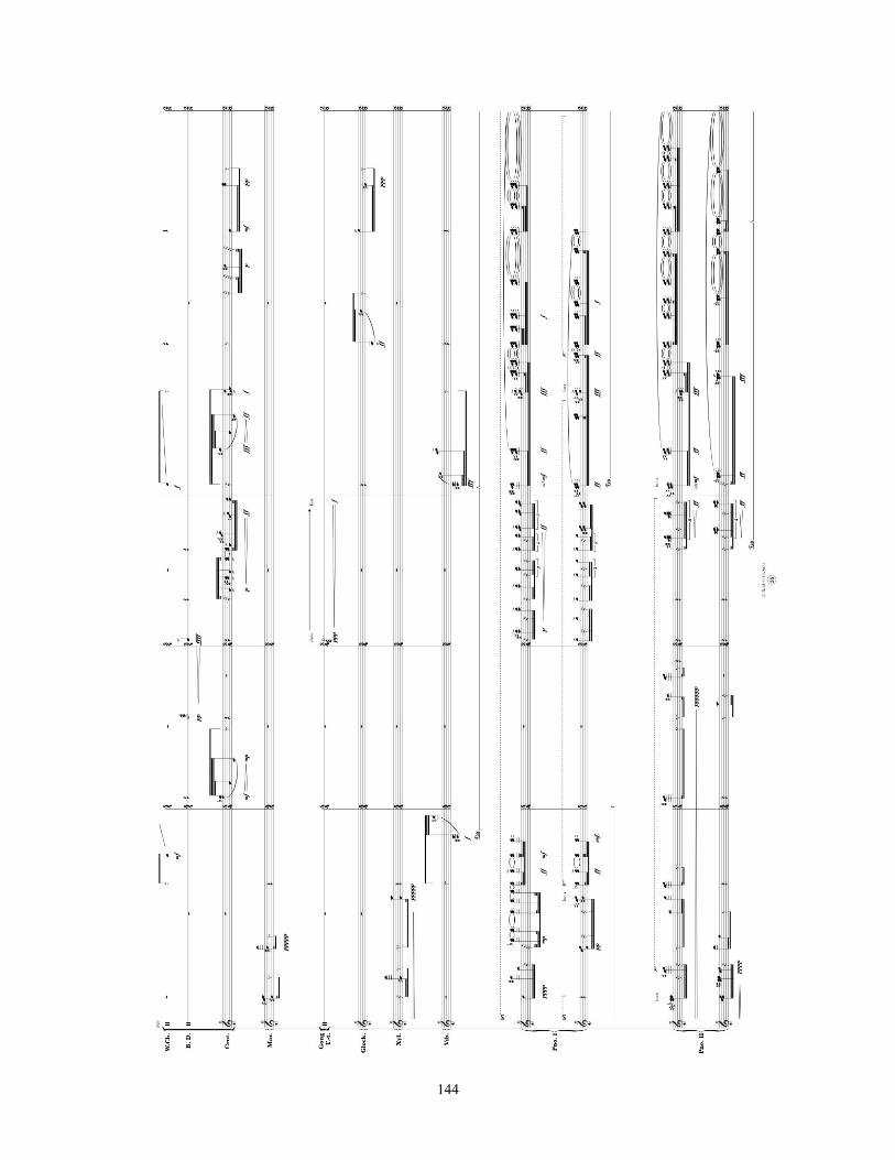
144

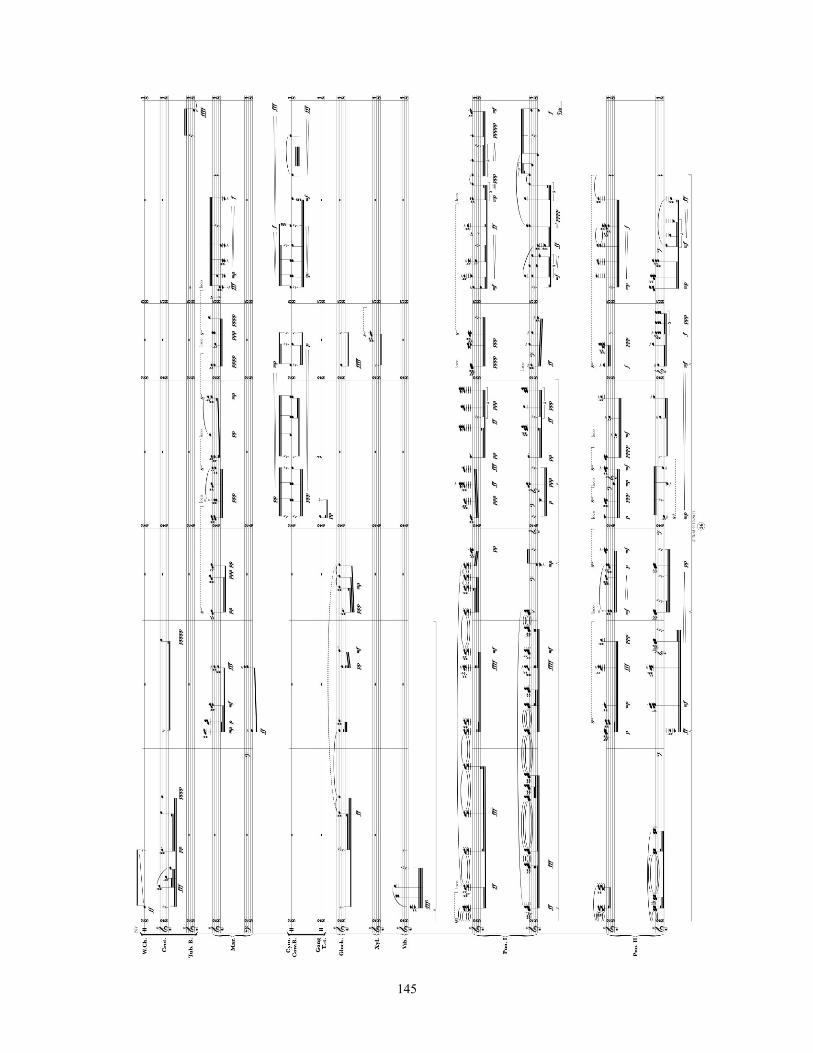
145

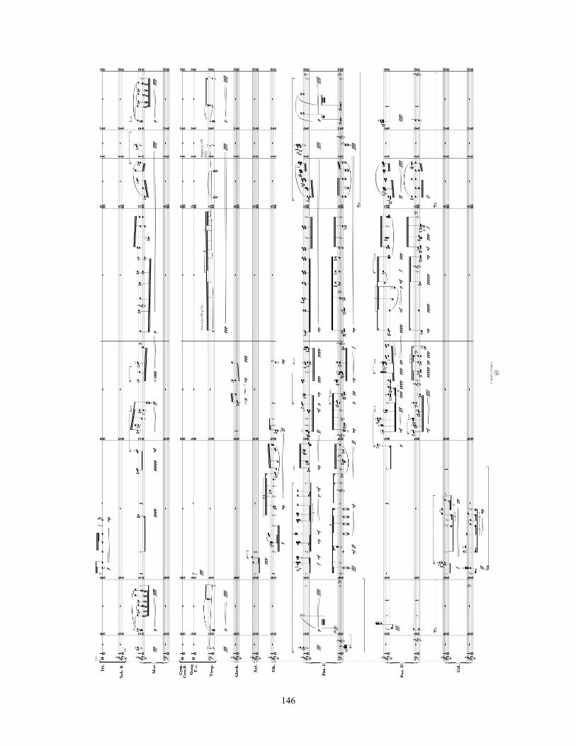
146

147

148

149

150

151

152

153

Bibliography

Abel, J. S., & Huang, P. (2006). A Simple, Robust Measure of Reverberation Echo Density. In Proceedings of the 121st AES Convention, 1–10.

Alberman, D. (2005). Abnormal Playing Techniques in the String Quartets of Helmut Lachenmann. Contemporary Music Review, 24(1), 39–51.

Anderson, J. (2000). A Provisional History of Spectral Music. Contemporary Music Review, 19(1989), 7–22.

ANSI, American National Standards Institute. (1960, (R1979)). 12.9 timbre. ANSI S1.1.

Aucouturier, J. (2006). Ten experiments on the modeling of polyphonic timbre. PhD thesis, L’Université Paris 6, Paris, France.

Bismarck, G. V. (1974). Sharpness as an Attribute of the Timbre of Steady Sounds. Acustica, 30.

Bismarck, G. V. (1974). Timbre of steady sounds: A factorial investigation of its verbal attributes. Acustica, 30, 146–59.

Blume, P. (2008). Mathias Spahlinger’s 128 erfüllte augenblicke and the Parameters of Listening. Contemporary Music Review, 27(6), 625–642.

Boulez, P. (1987). Timbre and composition–timbre and language. Contemporary Music Review, 2(1), 161–171.

Castanet, P. A., & Fineberg, J. (2000). Gérard Grisey and the Foliation of Time. Contemporary Music Review, 19(3), 29–40.

Erickson, R. (1975). Sound structure in music. Berkeley: University of California Press.

D’Escrivan, J. (1989). Reflections on the poetics of time in electroacoustic music. Contemporary Music Review, 3(1), 197–201.

Daubresse, E., Assayag, G., & Fineberg, J. (2000). Technology and creation — The creative evolution. Contemporary Music Review, 19(2), 61–80.

Feron, F.-X. (2012). The Emergence of Spectra in Gérard Grisey’s Compositional Process: From Dérives (1973-74) to Les espaces acousiques (1974-85). Contemporary Music Review, 30(5), 343–375.

Fineberg, J. (2000a). Appendix I: Guide to the Basic Concepts and Techniques of Spectral Music. Contemporary Music Review, 19(2), 81–113.

154

Fineberg, J. (2000b). Appendix II: Musical Examples. Contemporary Music Review, 19(1975), 115–134.

Fineberg, J. (2000c). Spectral music. Contemporary Music Review, 19(2), 1–5.

Fletcher, H. B. T. L. (1934). Loudness, Pitch and the Timbre of Musical Tones and Their Relation to the Intensity, the Frequency and the Overtone Structure. October, 6(2), 59–69.

Gayou, É. (2007). The GRM: landmarks on a historic route. Organised Sound, 12(03), 203–211.

Giordano, B. L., & McAdams, S. (2006). Material identification of real impact sounds: Effects of size variation in steel, glass, wood, and plexiglass plates. The Journal of the Acoustical Society of America, 119(2), 1171–1181.

Grella-Możejko, P. (2005). Helmut Lachenmann—Style, Sound, Text. Contemporary Music Review, 24(1), 57–75.

Grey, J. M. (1975). An exploration of musical timbre. PhD thesis, Stanford University, Center for Computer Research in Music and Acoustics, Report No. STAN-M-2.

Grey, J. M. (1977). Multidimensional perceptual scaling of musical timbres. The Journal of the Acoustical Society of America, 61(5), 1270–7.

Grey, J. M., & Gordon, J. W. (1978). Perceptual effects of spectral modifications on musical timbres. Journal of the Acoustical Society of America, 63(5), 1493–1500.

Grey, J. M. & Moorer, J.A. (1977). Perceptual evaluations of synthesized musical instrument tones. The Journal of the Acoustical Society of America, 62(2).

Grisey, G. (1987). Tempus ex Machina: A composer’s reflections on musical time. Contemporary Music Review, 2, 239–275.

Grisey, G., & Fineberg, J. (2000). Did You Say Spectral? Contemporary Music Review, 19(3), 1–3.

Hall, M. D., & Beauchamp, J. W. (2009). Clarifying spectral and temporal dimensions of musical instrument timbre. Acoustique Canadienne, Journal of the Canadian Acoustical Association, 37(1), 3–22.

Helmholtz, H. L. F. (Original German Edition in 1863, English translation in 1954). On the Sensation of Tone. Mineola, NY: Dover Publications.

155

Harvey, J. (1981). “Mortuos Plango, Vivos Voco”: A Realization at IRCAM. Computer Music Journal, 5(4), 22–24.

Harvey, J. (2001). Spectralism. Contemporary Music Review, 19(3), 11–14.

Heald, D. The Deutsche Bank Series at the Guggenheim Anish Kapoor Memory. Guggenheim. 2008. Retrieved May 31, 2013, from http://web.guggenheim.org/exhibitions/kapoor/index2.html

Huang, P. and Abel, J. (2007). Aspects of reverberation echo density. In Proceedings of the 121st AES Convention, Reprint 7163.

Huang, P., Abel, J. S., Terasawa, H., & Berger, J. (2008). Reverberation Echo Density Psychoacoustics. Audio Engineering Society Convention 125. Audio Engineering Society.

Irino, T., & Patterson, R. D. (2002). Segregating information about the size and shape of the vocal tract using a time-domain auditory model: The stabilised wavelet-Mellin transform. Speech Communication, 36(3-4), 181–203.

Iverson, P., & Krumhansl, C. L. (1993). Isolating the dynamic attributes of musical timbre. The Journal of the Acoustical Society of America, 94(5), 2595–603.

Klein, W., Plomp, R., & Pols, L. C. (1970). Vowel spectra, vowel spaces, and vowel identification. Journal of the Acoustical Society of America, 48(4), 999–1009.

Lakatos, S. (2000). A common perceptual space for harmonic and percussive timbres. Perception & psychophysics, 62(7), 1426–39.

Lalitte, P. (2011). The theories of Helmholtz in the work of Varese. Contemporary Music Review, 30(5), 329–344.

Ledoux, C., & Fineberg, J. (2000). From the philosophical to the Practical: An imaginary proposition concerning the music of Tristan Murail. Contemporary Music Review, 19(3), 41–65.

Lerdahl, F. (1987). Timbral hierarchies. Contemporary Music Review, 2(1), 135–160.

Malherbe, C., Fineberg, J., & Hayward, B. (2000). Seeing light as color; hearing sound as timbre. Contemporary Music Review, 19(3), 15–27.

Manning, P. (2013). Electronic and Computer Music. Oxford University Press.

Manoury, P. (1984). The arrow of time. Contemporary Music Review, 1(1), 131–145.

156

McAdams, S., & Cunible, J.-C. (1992). Perception of timbral analogies. Philosophical transactions: Biological sciences, Processing of Complex Sounds by the Auditory System, 336(1278), 383–389.

McAdams, S., Giordano, B., Susini, P., Peeters, G., & Rioux, V. (2006). A meta-analysis of acoustic correlates of timbre dimensions [Lecture slides]. Retrieved from McGill University: http://www.dafx.ca/slides/keynote3.pdf

McAdams, S., & Saariaho, K. (1985). Qualities and Functions of Musical Timbre. International Computer Music Conference, 367–374.

McAdams, S., Winsberg, S., Donnadieu, S., De Soete, G., & Krimphoff, J. (1995). Perceptual scaling of synthesized musical timbres: common dimensions, specificities, and latent subject classes. Psychological Research, 58(3), 177–192.

Mirka, D. (2012). To cut the Gordian Knot: the timbre system of Krzysztof Penderecki. Journal of Music Theory, 45(2), 435–456.

Murail, T. (2000). After-thoughts. Contemporary Music Review, 19(3), 5–9.

Murail, T. (2005c). The Revolution of Complex Sounds. Contemporary Music Review, 24(2-3), 121–135.

Murail, T. (2005d). Spectra and Sprites. Contemporary Music Review, 24(2-3), 137–147.

Pasler, J. (1982). Debussy, “Jeux”: Playing with Time and Form. 19th Century Music, 6(1), 60–75.

Peeters, G., Giordano, B. L., Susini, P., Misdariis, N., & McAdams, S. (2011). The Timbre Toolbox: extracting audio descriptors from musical signals. The Journal of the Acoustical Society of America, 130(5), 2902–16.

Peterson, G. E. (1952). Control Methods Used in a Study of the Vowels. The Journal of the Acoustical Society of America, 24(2), 175.

Plomp, R. (1976). Aspects of tone sensation: a psychophysical study. Academic Press.

Pollard, H. F., & Jansson, E. V. (1982). A Tristimulus Method for the Specification of Musical Timbre. International Journal of Acoustics, 51, 162–171.

Poli, G. D., & Prandoni, P. (1997). Sonological models for timbre characterization. Journal of New Music Research, 26(2), 170–197.

Pousset, D., Fineberg, J., & Hyacinthe, R. (2000). The Works of Kaija Saariaho, Philippe Hurel and Marc-André Dalbavie—Stile Concertato, Stile Concitato, Stile Rappresentativo. Contemporary Music Review, 19(3), 67–110.

157

Pratt, R. (1976). A subjective rating scale for timbre. Journal of Sound and Vibration, 45(3), 317–328.

Puckette, M. (2007). The theory and technique of electronic music. Hackensack, N.J: World Scientific Publishing Co.

Risset, J. C. (1994). Sculpting sounds with computers: music, science, technology. Leonardo, 27(3), 257–261.

Risset, J. C. (2002). Electroacoustic Music: Analytical Perspectives. London, UK: Greenwood Press.

Risset, J. C., & Wessel, D. (1999). Exploration of Timbre by Analysis Synthesis. The Psychology of Music. San Diego: Academic Press.

Rose, F. (1996). Introduction to the pitch organization of French spectral music. Perspectives of New Music, 34(2), 6–39.

Rose, F., & Kapuscinski, J. (2009). Japanese Traditional Orchestral Music: The Correlation between Time and Timbre. In Proceedings from the Conference of Interdisciplinary Musicology, 1–6.

Rossing, T. (1990). The science of sound. Reading, Mass.: Addison-Wesley Pub. Co.

Rossing, T.D. (2012). Pitch and Timbre. Lecture conducted from Stanford University, CA.

Saariaho, K. (1987). Timbre and harmony: Interpolations of timbral structures. Contemporary Music Review, 2(1), 93–133.

Schaeffer, P. (1966). Traité des objets musicaux, essai interdisciplines. Paris: Éditions du Seuil.

Schubert, E., & Wolfe, J. (2006). Does Timbral Brightness Scale with Frequency and Spectral Centroid? ACTA Acustica United with Acustica, 92(5), 820–825.

Stephenson, R. B., & Seiberling, C. L. (1994). Jaffrey then and now: Changes in community character. Jaffrey, N.H: Jaffrey Historic District Commission.

Singh, S., & Woods, D. R. (1971). Perceptual structure of 12 American English vowels. The Journal of the Acoustical Society of America, 49(6), 1861–6.

Slawson, W. (1985). Sound color. Berkeley: University of California Press.

158

Smalley, D. (1997). Spectromorphology: explaining sound-shapes. Organised Sound, 2(2), 107–126.

Spahlinger, M. (2008). This Is the Time of Conceptive Ideologues No Longer. Contemporary Music Review, 27(6), 579–594.

Steenhuisen, P. (2004). Interview with Helmut Lachenmann—Toronto, 2003. Contemporary Music Review, 23(3-4), 9–14.

Sundberg, J. (1977). Vibrato and vowel identification. Arch Acoust, 2, 257–266.

Surianu, H., & Fineberg, J. (2000). Romanian spectral music or another expression freed. Contemporary Music Review, 19(2), 23–32.

Terasawa, H. (2009). A Hybrid Model for Timbre Perception: Quantitative Representations of Sound, Color, and Density. PhD thesis, Stanford University, Center for Computer Research in Music and Acoustics.

Terasawa, H., Slaney, M., & Berger, J. (2005a). A Timbre Space for Speech. Interspeech, 4–7.

Terasawa, H., Slaney, M., & Berger, J. (2005b). Perceptual Distance in Timbre Space. Eleventh Meeting of the International Converence on Auditory Display, 5, 61–68. Limerick, Ireland.

Terasawa, H., Slaney, M., & Berger, J. (2005c). The Thirteen Colors of Timbre. 2005 IEEE Workshop on Applications of Signal Processing to Audio and Acoustics, 323–326. New Paltz, NY: IEEE.

Traube, C. (2006). Instrumental and Vocal Timbre Perception [Lecture slides]. Retrieved from the University of Graz Psychology of Music Performance Seminar: http://www.uni-graz.at/richard.parncutt/guests/2006/traube/Slides_CTraube_timbre.pdf

Traube, C., & Depalle, P. (2004). Phonetic gestures underlying guitar timbre description. Proceedings of the International Conference on Music Perception and Cognition,658–661.

Vassilakis, P. N. (1995). Introduction to Psychoacoustics and Sound Perception—Timbre. Retrieved from http://acousticslab.org/psychoacoustics/

Wessel, D. L. (1979). Timbre Space as a Musical Control Structure. (C. Roads & J. Strawn, Eds.) Computer Music Journal, 3(2), 45–52.

Wishart, T., & Emmerson, S. (1996). On sonic art. Amsterdam: Harwood Academic Publishers.

159