Composer Classification Models for Music-Theory Building

Chapter 14Composer Classification Models forMusic-Theory Building

Dorien Herremans, David Martens, and Kenneth Sorensen

Abstract The task of recognizing a composer by listening to a musical piece usedto be reserved for experts in music theory. The problems we address here are, first,that of constructing an automatic system that is able to distinguish between musicwritten by different composers; and, second, identifying the musical properties thatare important for this task. We take a data-driven approach by scanning a largedatabase of existing music and develop five types of classification model that canaccurately discriminate between three composers (Bach, Haydn and Beethoven).More comprehensible models, such as decision trees and rulesets, are built, as wellas black-box models such as support vector machines. Models of the first type offerimportant insights into the differences between composer styles, while those of thesecond type provide a performance benchmark.

14.1 Introduction

Automatic composer-identification is a complex task that remains a challenge in thefield of music information retrieval (MIR). The problems we address here are, first,that of constructing an automatic system that is able to distinguish between musicwritten by different composers; and, second, that of identifying the musical propertiesthat are important for this task. The latter can offer interesting insights for musictheorists.

A data-driven approach is taken in this research by extracting global features froma large database of existing music. Based on this data, five types of classification

Dorien Herremans · Kenneth SorensenANT/OR, University of Antwerp Operations Research Group, Antwerp, Belgiume-mail: {dorien.herremans, kenneth.sorensen}@uantwerpen.be

David MartensApplied Data Mining Research Group, University of Antwerp, Antwerp, Belgiume-mail: [email protected]

369Preprint accepted for publication in the Springer bookon Computational Music Analysis, ISBN: 978-3-319-25929-1,

pages 369-392, Editor: David Meredith

370 Dorien Herremans, David Martens, and Kenneth Sorensen

model (decision tree, ruleset, logistic regression, support vector machines and NaiveBayes) are developed that can accurately classify a musical piece between Bach,Haydn or Beethoven. Most of the developed models are comprehensible and offerinsight into the styles of the composers. Yet, a few black-box models were also builtas a performance benchmark.

14.2 Prior Work in Music Information Retrieval

The task of composer classification belongs to the domain of Music InformationRetrieval (MIR), a multidisciplinary field concerned with retrieving and analysingmultifaceted information from large music databases (Downie, 2003). The field ofMIR has grown rapidly in recent years due to the digitization of the music industry.In 2011 alone, the European consumer expenditure on digital media exceeded 33billion euros (Stenzel and Downes, 2012).

The first mention of the term MIR is due to Kassler (1966), who named theprogramming language he developed to extract information from music files “MIR”.The early work done on the topic of computational music analysis is described inmore detail by Mendel (1969).

Recently, many topics have been explored in the field of MIR. Examples of theseare the content-based music search engine “query-by-humming”, which allows a userto hum a tune in order to search for the original song in a large database (Ghias et al.,1995; Tseng, 1999). Pfeiffer et al. (1997) developed a system that can detect violencein video soundtracks. The techniques developed by Wold et al. (1996) are used to, forinstance, identify different types of human speaker (e.g., female versus male). Musicsimilarity research is another topic that has been explored by MIR scientists, in whichthe similarity of two musical pieces is measured (Berenzweig et al., 2004). For moredetailed surveys of research done in the field of MIR, see Typke et al. (2005), Weihset al. (2007) and Casey et al. (2008). In the current chapter, however, the focus willbe on composer classification.

14.2.1 Classification Systems

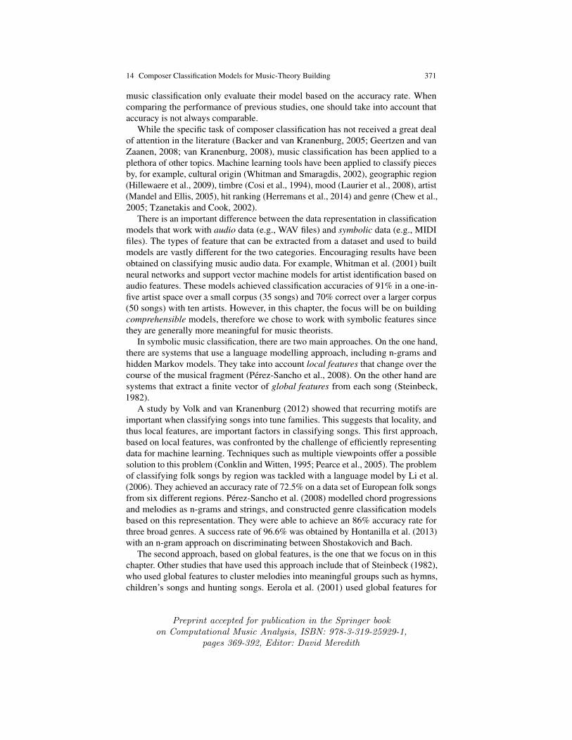
The task of music classification can be seen as building models that assign one ormore class labels to musical pieces based on their content. These models are oftenevaluated based on accuracy, i.e., the number of correctly classified instances versusthe total number of instances. It should be noted however that accuracy is not alwaysthe best performance measure, for instance in the case of an unbalanced dataset. Inthis research, the area under the curve (AUC) of the receiver operating characteristic(ROC) is used to evaluate the performance of the models. This metric, which takesinto account the true positives versus the false positives, is more suitable since thedataset is slightly skewed (see Fig. 14.1) (Fawcett, 2004). Most existing studies on

Preprint accepted for publication in the Springer bookon Computational Music Analysis, ISBN: 978-3-319-25929-1,


14 Composer Classification Models for Music-Theory Building 371

music classification only evaluate their model based on the accuracy rate. Whencomparing the performance of previous studies, one should take into account thataccuracy is not always comparable.

While the specific task of composer classification has not received a great dealof attention in the literature (Backer and van Kranenburg, 2005; Geertzen and vanZaanen, 2008; van Kranenburg, 2008), music classification has been applied to aplethora of other topics. Machine learning tools have been applied to classify piecesby, for example, cultural origin (Whitman and Smaragdis, 2002), geographic region(Hillewaere et al., 2009), timbre (Cosi et al., 1994), mood (Laurier et al., 2008), artist(Mandel and Ellis, 2005), hit ranking (Herremans et al., 2014) and genre (Chew et al.,2005; Tzanetakis and Cook, 2002).

There is an important difference between the data representation in classificationmodels that work with audio data (e.g., WAV files) and symbolic data (e.g., MIDIfiles). The types of feature that can be extracted from a dataset and used to buildmodels are vastly different for the two categories. Encouraging results have beenobtained on classifying music audio data. For example, Whitman et al. (2001) builtneural networks and support vector machine models for artist identification based onaudio features. These models achieved classification accuracies of 91% in a one-in-five artist space over a small corpus (35 songs) and 70% correct over a larger corpus(50 songs) with ten artists. However, in this chapter, the focus will be on buildingcomprehensible models, therefore we chose to work with symbolic features sincethey are generally more meaningful for music theorists.

In symbolic music classification, there are two main approaches. On the one hand,there are systems that use a language modelling approach, including n-grams andhidden Markov models. They take into account local features that change over thecourse of the musical fragment (Perez-Sancho et al., 2008). On the other hand aresystems that extract a finite vector of global features from each song (Steinbeck,1982).

A study by Volk and van Kranenburg (2012) showed that recurring motifs areimportant when classifying songs into tune families. This suggests that locality, andthus local features, are important factors in classifying songs. This first approach,based on local features, was confronted by the challenge of efficiently representingdata for machine learning. Techniques such as multiple viewpoints offer a possiblesolution to this problem (Conklin and Witten, 1995; Pearce et al., 2005). The problemof classifying folk songs by region was tackled with a language model by Li et al.(2006). They achieved an accuracy rate of 72.5% on a data set of European folk songsfrom six different regions. Perez-Sancho et al. (2008) modelled chord progressionsand melodies as n-grams and strings, and constructed genre classification modelsbased on this representation. They were able to achieve an 86% accuracy rate forthree broad genres. A success rate of 96.6% was obtained by Hontanilla et al. (2013)with an n-gram approach on discriminating between Shostakovich and Bach.

The second approach, based on global features, is the one that we focus on in thischapter. Other studies that have used this approach include that of Steinbeck (1982),who used global features to cluster melodies into meaningful groups such as hymns,children’s songs and hunting songs. Eerola et al. (2001) used global features for




assessing similarity. Ponce de Leon and Inesta (2003) used global melodic, harmonicand rhythmic descriptors for style classification. The ensemble method based on aneural network and a k-nearest neighbour developed by McKay and Fujinaga (2004)for genre classification used 109 global features and achieved an accuracy of 98% forroot genres and 90% for leaf genres. Moreno-Seco et al. (2006) also applied ensemblemethods based on global features to a style classification problem. Bohak and Marolt(2009) used the same type of features to assess the similarity between Slovenianfolk song melodies. Herlands et al. (2014) combined typical global features with anovel class of local features to detect nuanced stylistic elements. Their classificationmodels obtained an accuracy of 80% when discriminating between Haydn’s andMozart’s string quartets.

A small number of studies have compared both types of feature and comparedtheir performance on the folk music classification problem. Jesser (1991) createdclassification models based on both features using the dataset from Steinbeck (1982).Her conclusion was that global features do not contribute much to the classification.A study by Hillewaere et al. (2009) found that event models outperform a globalfeature approach for classifying folk songs by their geographical origin (England,France, Ireland, Scotland, South East Europe and Scandinavia). In another studywith European folk tunes, Hillewaere et al. (2012) compared string methods withn-gram models and global features for genre classification of 9 dance types. Theyconcluded that features based on duration lead to better classification, no matterwhich method is used, although the n-gram method performed best overall. VanKranenburg et al. (2013) obtained similar results for the classification of Dutch folktunes into tune families. Their study showed that local features always obtain thebest results, yet global features can be successful on a small corpus when the optimalsubset of features is used. Similar results were obtained in a study to detect similaritybetween folk tunes (van Kranenburg, 2010).

Since the dataset used in our research was relatively small and global featureswere a relatively simple way of representing melodies that can be easily processed bydifferent types of classifier, we opted to use a carefully selected set of global featuresin the research reported in this chapter.

14.2.2 Composer Classification

While a lot of research has been done on the task of automatic music classification (seeSect. 14.2.1), the subtask of composer classification remains relatively unexplored.

Wołkowicz et al. (2007) used n-grams to classify piano files into groups of fivecomposers. Hillewaere et al. (2010) also used n-grams and compared them withglobal feature models to distinguish between string quartets by Haydn and Mozart.The classification accuracy of their trigram approach for recognizing composers forstring quartets was 61% for violin and viola, and 75% for cello. Another system thatclassifies string quartet pieces by composer has been implemented by Kaliakatsos-Papakostas et al. (2011). They used a Markov chain to represent the four voices of




the quartets as a monophonic melody. A classification success rate of 59 to 88%was achieved when classifying between two composers with their weighted Markovchain model. The study performed by Pollastri and Simoncelli (2001) had a loweraccuracy rate than the previously discussed research. The Hidden Markov Modelsthey designed for the classification of 605 monophonic themes by five composershad an accuracy of 42% on average. Backer and van Kranenburg (2005) have appliedstatistical pattern recognition to the problem of distinguishing Bach from Handel,Telemann, Haydn and Mozart using 20 features in different time slices throughoutthe pieces. They concluded that it is “very possible to isolate the style of J.S. Bachfrom Telemann, Handel, Haydn or Mozart”.

Van Kranenburg and Backer (2004) used 20 global style markers based on proper-ties of counterpoint. A decision tree (C4.5) (Quinlan, 1993) and nearest neighbourclassification algorithm are built on a database of 320 pieces from the eighteenth andearly nineteenth century. They are able to achieve a fairly low error rate. Althoughthe features are described in the paper, a detailed description of the models is missing.Similar features based on counterpoint are used by Mearns et al. (2010) to developa C4.5 decision tree and naive Bayes models. Their models correctly classified 44out of 66 pieces with 7 groups of composers. The resulting decision tree could givemusic theorists insight into the differences between styles of composers; however,the tree is not shown in the paper.

In the following sections, the dataset used in this research is discussed togetherwith the chosen features. These are then used to build accurate and comprehensibleclassification models (Sect. 14.4). The resulting models are described in detail in thischapter and give insight into the differences between the styles of Haydn, Beethovenand Bach.

14.3 Data Sources

The range of features that can be extracted from music depends heavily on the typeof file they have to be extracted from. Computational music analysis is typicallyperformed on two types of music file, those based on audio signals and structuredfiles. The first category includes files representing audio signals (e.g., WAV and MP3)and files containing the values of features derived from audio signals (e.g., short-termFourier spectra, MFCCs, etc.). While there is a large quantity of music available insuch formats, the types of feature that result from analysing these files (e.g., spectralflux and zero-crossing rate (Tzanetakis et al., 2003)) are not the most comprehensible,especially for music theorists. For the purpose of our research, it was therefore moreappropriate to work with files of the second type, i.e., structured files.

Structured, symbolic files, such as MIDI files, contain high-level structured infor-mation about music. MIDI files, in particular, describe a specific way of performinga piece and contain information such as the start, duration, velocity and instrumentof each note. These files allow us to extract musically meaningful features.




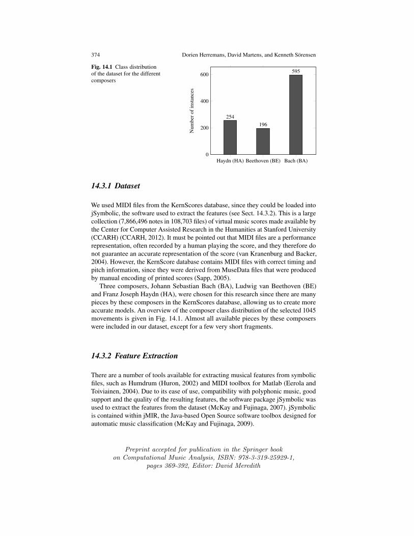
Fig. 14.1 Class distributionof the dataset for the differentcomposers

Haydn (HA) Beethoven (BE) Bach (BA)0

200

400

600

254196

595

Num

bero

fins

tanc

es14.3.1 Dataset

We used MIDI files from the KernScores database, since they could be loaded intojSymbolic, the software used to extract the features (see Sect. 14.3.2). This is a largecollection (7,866,496 notes in 108,703 files) of virtual music scores made available bythe Center for Computer Assisted Research in the Humanities at Stanford University(CCARH) (CCARH, 2012). It must be pointed out that MIDI files are a performancerepresentation, often recorded by a human playing the score, and they therefore donot guarantee an accurate representation of the score (van Kranenburg and Backer,2004). However, the KernScore database contains MIDI files with correct timing andpitch information, since they were derived from MuseData files that were producedby manual encoding of printed scores (Sapp, 2005).

Three composers, Johann Sebastian Bach (BA), Ludwig van Beethoven (BE)and Franz Joseph Haydn (HA), were chosen for this research since there are manypieces by these composers in the KernScores database, allowing us to create moreaccurate models. An overview of the composer class distribution of the selected 1045movements is given in Fig. 14.1. Almost all available pieces by these composerswere included in our dataset, except for a few very short fragments.

14.3.2 Feature Extraction

There are a number of tools available for extracting musical features from symbolicfiles, such as Humdrum (Huron, 2002) and MIDI toolbox for Matlab (Eerola andToiviainen, 2004). Due to its ease of use, compatibility with polyphonic music, goodsupport and the quality of the resulting features, the software package jSymbolic wasused to extract the features from the dataset (McKay and Fujinaga, 2007). jSymbolicis contained within jMIR, the Java-based Open Source software toolbox designed forautomatic music classification (McKay and Fujinaga, 2009).




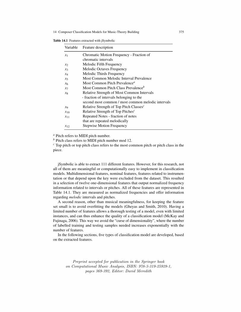
Table 14.1 Features extracted with jSymbolic

Variable Feature description

x1 Chromatic Motion Frequency - Fraction ofchromatic intervals

x2 Melodic Fifth Frequencyx3 Melodic Octaves Frequencyx4 Melodic Thirds Frequencyx5 Most Common Melodic Interval Prevalencex6 Most Common Pitch Prevalencea

x7 Most Common Pitch Class Prevalenceb

x8 Relative Strength of Most Common Intervals- fraction of intervals belonging to thesecond most common / most common melodic intervals

x9 Relative Strength of Top Pitch Classesc

x10 Relative Strength of Top Pitchesc

x11 Repeated Notes - fraction of notesthat are repeated melodically

x12 Stepwise Motion Frequency

a Pitch refers to MIDI pitch number.b Pitch class refers to MIDI pitch number mod 12.c Top pitch or top pitch class refers to the most common pitch or pitch class in thepiece.

jSymbolic is able to extract 111 different features. However, for this research, notall of them are meaningful or computationally easy to implement in classificationmodels. Multidimensional features, nominal features, features related to instrumen-tation or that depend upon the key were excluded from the dataset. This resultedin a selection of twelve one-dimensional features that output normalized frequencyinformation related to intervals or pitches. All of these features are represented inTable 14.1. They are measured as normalized frequencies and offer informationregarding melodic intervals and pitches.

A second reason, other than musical meaningfulness, for keeping the featureset small is to avoid overfitting the models (Gheyas and Smith, 2010). Having alimited number of features allows a thorough testing of a model, even with limitedinstances, and can thus enhance the quality of a classification model (McKay andFujinaga, 2006). This way we avoid the “curse of dimensionality”, where the numberof labelled training and testing samples needed increases exponentially with thenumber of features.

In the following sections, five types of classification model are developed, basedon the extracted features.




14.4 Classification Models

Predictive models can be used not only for classification, but also in theory-buildingand testing (Shmueli and Koppius, 2011). Using powerful models, in combinationwith high-level musical features enables us to construct models that give usefulinsights into the characteristics of the style of a composer. The first models in thissection (i.e., rulesets and trees) are of a more linguistic nature and therefore fairlyeasy to understand (Martens, 2008). Support vector machines and naive Bayes classi-fiers are more black-box, as they provide a complex non-linear output score. Usingpedagogical rule extraction techniques like Trepan and G-REX (Martens et al., 2007),comprehensible rulesets can still be extracted from black-box models. However, thisfalls outside the scope of this chapter. The ruleset described in Sect. 14.4.2 simplyinduces the rules directly from the data. While this research focuses on building com-prehensible models, some black-box models were included to provide performancebenchmarks.

The open source software, Weka, is used to create five different types of classifica-tion model, each with varying levels of comprehensibility, using supervised learningtechniques (Witten and Frank, 2005). This toolbox and framework for data miningand machine learning is a landmark system in this field (Hall et al., 2009). jSymbolic,used to extract features as described in Sect. 14.3.2 above, outputs the features of allinstances in ACE XML files. The jMIR toolbox offers a tool to convert these featuresinto Weka ARFF format (McKay and Fujinaga, 2008).

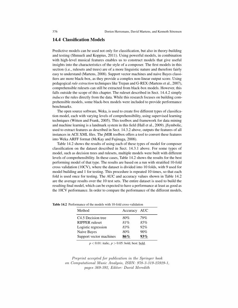
Table 14.2 shows the results of using each of these types of model for composerclassification on the dataset described in Sect. 14.3.1 above. For some types ofmodel, such as decision trees and rulesets, multiple models were built with differentlevels of comprehensibility. In these cases, Table 14.2 shows the results for the bestperforming model of that type. The results are based on a run with stratified 10-foldcross validation (10CV), where the dataset is divided into 10 folds, with 9 used formodel building and 1 for testing. This procedure is repeated 10 times, so that eachfold is used once for testing. The AUC and accuracy values shown in Table 14.2are the average results over the 10 test sets. The entire dataset is used to build theresulting final model, which can be expected to have a performance at least as good asthe 10CV performance. In order to compare the performance of the different models,

Table 14.2 Performance of the models with 10-fold cross-validation

Method Accuracy AUC

C4.5 Decision tree 80% 79%RIPPER ruleset 81% 85%Logistic regression 83% 92%Naive Bayes 80% 90%Support vector machines 86% 93%

p < 0.01: italic, p > 0.05: bold, best: bold.




a Wilcoxon signed-rank test was conducted, the null hypothesis of this test being thatthere is no difference between the performance of a model and that of the best model.

14.4.1 C4.5 Tree

In this section we describe a decision tree classifier, which is a simple, yet widelyused and comprehensible classification technique. Even though decision trees are notalways the most competitive models in terms of accuracy, they are computationallyefficient and offer a visual understanding of the classification process. A decision treeis a tree data structure that consists of decision nodes and leaves, where the leavesspecify the class value (i.e., composer) and the nodes specify a test of one of thefeatures. A predictive rule is found by following a path from the root to a leaf basedon the feature values of a particular piece. The resulting leaf indicates the predictedcomposer for that particular piece (Ruggieri, 2002).

J48 (Witten and Frank, 2005), Weka’s implementation of the C4.5 algorithm, isused to build decision trees (Quinlan, 1993). A “divide and conquer” approach is usedby C4.5 to build trees recursively. This is a top-down approach, which repeatedlyseeks a feature that best separates the classes, based on normalized information gain(i.e., difference in entropy). After this step, subtree raising is done by pruning thetree from the leaves to the root (Wu et al., 2008).

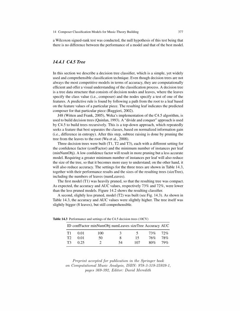
Three decision trees were built (T1, T2 and T3), each with a different setting forthe confidence factor (confFactor) and the minimum number of instances per leaf(minNumObj). A low confidence factor will result in more pruning but a less accuratemodel. Requiring a greater minimum number of instances per leaf will also reducethe size of the tree, so that it becomes more easy to understand; on the other hand, itwill also reduce accuracy. The settings for the three trees are shown in Table 14.3,together with their performance results and the sizes of the resulting trees (sizeTree),including the numbers of leaves (numLeaves).

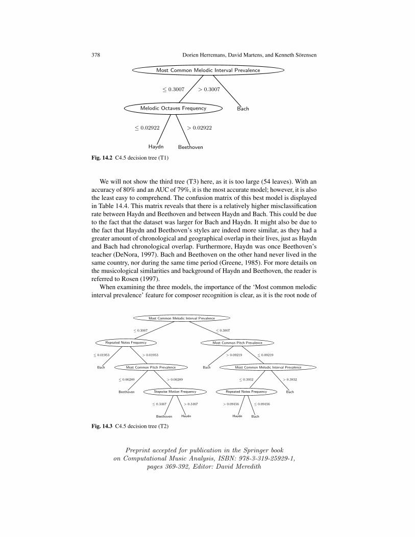
The first model (T1) was heavily pruned, so that the resulting tree was compact.As expected, the accuracy and AUC values, respectively 73% and 72%, were lowerthan the less pruned models. Figure 14.2 shows the resulting classifier.

A second, slightly less pruned, model (T2) was built (see Fig. 14.3). As shown inTable 14.3, the accuracy and AUC values were slightly higher. The tree itself wasslightly bigger (8 leaves), but still comprehensible.

Table 14.3 Performance and settings of the C4.5 decision trees (10CV)

ID confFactor minNumObj numLeaves sizeTree Accuracy AUC

T1 0.01 100 3 5 73% 72%T2 0.01 50 8 15 76% 78%T3 0.25 2 54 107 80% 79%




Most Common Melodic Interval Prevalence

Melodic Octaves Frequency

≤ 0.3007

Haydn

≤ 0.02922

Beethoven

> 0.02922

Bach

> 0.3007

Fig. 14.2 C4.5 decision tree (T1)

We will not show the third tree (T3) here, as it is too large (54 leaves). With anaccuracy of 80% and an AUC of 79%, it is the most accurate model; however, it is alsothe least easy to comprehend. The confusion matrix of this best model is displayedin Table 14.4. This matrix reveals that there is a relatively higher misclassificationrate between Haydn and Beethoven and between Haydn and Bach. This could be dueto the fact that the dataset was larger for Bach and Haydn. It might also be due tothe fact that Haydn and Beethoven’s styles are indeed more similar, as they had agreater amount of chronological and geographical overlap in their lives, just as Haydnand Bach had chronological overlap. Furthermore, Haydn was once Beethoven’steacher (DeNora, 1997). Bach and Beethoven on the other hand never lived in thesame country, nor during the same time period (Greene, 1985). For more details onthe musicological similarities and background of Haydn and Beethoven, the reader isreferred to Rosen (1997).

When examining the three models, the importance of the ‘Most common melodicinterval prevalence’ feature for composer recognition is clear, as it is the root node of


Repeated Notes Frequency

≤ 0.3007

Bach

≤ 0.01953

Most Common Pitch Prevalence

> 0.01953

Beethoven

≤ 0.06289

Stepwise Motion Frequency

> 0.06289

Beethoven

≤ 0.3467

Haydn

> 0.3467

Most Common Pitch Prevalence

≤ 0.3007

Bach

> 0.09219


≤ 0.09219

Repeated Notes Frequency

≤ 0.3932

Haydn

> 0.09456

Bach

≤ 0.09456

Bach

> 0.3932

Fig. 14.3 C4.5 decision tree (T2)




all three models. It indicates that Bach focuses more on one particular interval thanthe other composers. Bach also seems to use fewer repeated notes than the other twocomposers. The ‘Melodic octaves frequency’ feature indicates that Beethoven usesmore octaves in melodies than Haydn.

14.4.2 RIPPER

As with the decision trees just described, the rulesets presented in this section werebuilt with an inductive rule-learning algorithm (as opposed to rule-extraction tech-niques such as Trepan and G-REX (Martens et al., 2007)). They are comprehensiblemodels based on “if-then” rules, that are computationally efficient to implement.

JRip, Weka’s implementation of the ‘Repeated Incremental Pruning to ProduceError Reduction’ (RIPPER) algorithm, was used to build a ruleset for composerclassification (Cohen, 1995). RIPPER uses sequential covering to generate the ruleset.It consists of a building stage and an optimization stage. The building stage starts bygrowing one rule by greedily adding antecedents (or conditions) to the rule, until it isperfect (i.e., 100% accurate) based on an initial growing and pruning set (ratio 2:1).The algorithm tries every possible value for each attribute and selects the conditionwith the highest information gain. Then each condition is pruned in last-to-first order.This is repeated until either there are no more positive examples, or the descriptionlength (DL) is 64 bits greater than the smallest DL found so far, or the error rate is>50%. In the optimization phase, the instances covered by existing rules are removedfrom the pruning set. Based on this new pruning set, each rule is reconsidered andtwo variants are produced. If one of the variants offers a better description length, itreplaces the rule. This process is repeated (Hall et al., 2009). The models below werecreated with 50 optimizations.

We again built three models (R1, R2 and R3), each with varying levels of com-plexity. This was achieved by varying the minimum total weight of the instances in arule (minNo). Setting a higher level for this parameter forces the algorithm to havemore instances for each rule, thus reducing the total number of rules in the model.The settings and performance results of the models are summarized in Table 14.5.

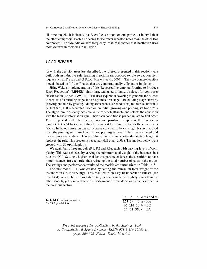
The first model (R1) was created by setting the minimum total weight of theinstances in a rule very high. This resulted in an easy-to-understand ruleset (seeFig. 14.4). As can be seen in Table 14.5, its performance is slightly lower than theother models, yet comparable to the performance of the decision trees, described inthe previous section.

Table 14.4 Confusion matrixfor C4.5 (model T3)

a b c classified as175 39 40 a = HA66 110 20 b = BE24 21 550 c = BA




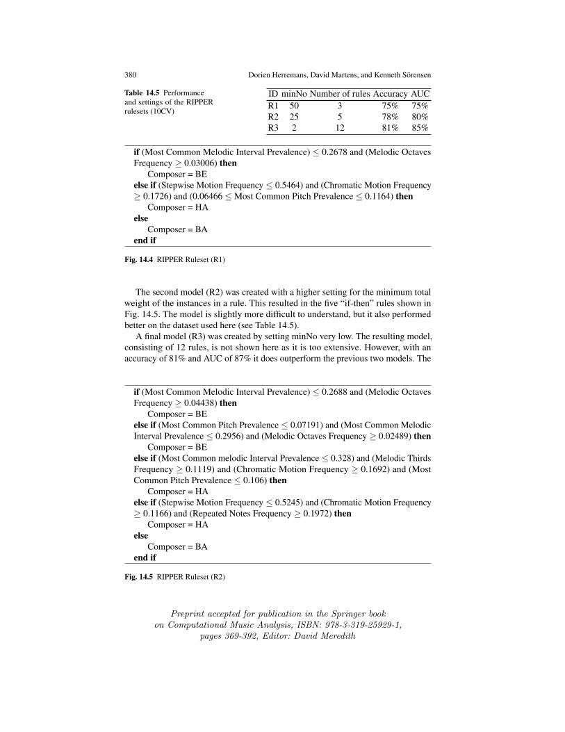
Table 14.5 Performanceand settings of the RIPPERrulesets (10CV)

ID minNo Number of rules Accuracy AUCR1 50 3 75% 75%R2 25 5 78% 80%R3 2 12 81% 85%

if (Most Common Melodic Interval Prevalence) ≤ 0.2678 and (Melodic OctavesFrequency ≥ 0.03006) then

Composer = BEelse if (Stepwise Motion Frequency ≤ 0.5464) and (Chromatic Motion Frequency≥ 0.1726) and (0.06466 ≤Most Common Pitch Prevalence ≤ 0.1164) then

Composer = HAelse

Composer = BAend if

Fig. 14.4 RIPPER Ruleset (R1)

The second model (R2) was created with a higher setting for the minimum totalweight of the instances in a rule. This resulted in the five “if-then” rules shown inFig. 14.5. The model is slightly more difficult to understand, but it also performedbetter on the dataset used here (see Table 14.5).

A final model (R3) was created by setting minNo very low. The resulting model,consisting of 12 rules, is not shown here as it is too extensive. However, with anaccuracy of 81% and AUC of 87% it does outperform the previous two models. The

if (Most Common Melodic Interval Prevalence) ≤ 0.2688 and (Melodic OctavesFrequency ≥ 0.04438) then

Composer = BEelse if (Most Common Pitch Prevalence ≤ 0.07191) and (Most Common MelodicInterval Prevalence ≤ 0.2956) and (Melodic Octaves Frequency ≥ 0.02489) then

Composer = BEelse if (Most Common melodic Interval Prevalence ≤ 0.328) and (Melodic ThirdsFrequency ≥ 0.1119) and (Chromatic Motion Frequency ≥ 0.1692) and (MostCommon Pitch Prevalence ≤ 0.106) then

Composer = HAelse if (Stepwise Motion Frequency ≤ 0.5245) and (Chromatic Motion Frequency≥ 0.1166) and (Repeated Notes Frequency ≥ 0.1972) then

Composer = HAelse

Composer = BAend if

Fig. 14.5 RIPPER Ruleset (R2)




Table 14.6 Confusion matrixfor RIPPER


confusion matrix of the model is shown in Table 14.6. The misclassification ratesare very similar to those of the decision trees in the previous section, with fewestmisclassifications occurring between Beethoven and Bach.

It is noticeable that the first feature evaluated by the rulesets is the same as theroot feature of the decision trees in Sect. 14.4.1 above, which confirms its importance.The rulesets and decision trees can be interpreted in a similar way. Like the decisiontrees, the rulesets suggest that Beethoven uses more melodic octaves than the othercomposers and that Haydn uses more repeated notes than Bach.

14.4.3 Logistic Regression

In the previous sections, two techniques were explored to build comprehensiblemodels. Both trees and rulesets provide crisp classification. This means that theyclassify a musical piece as being either by a certain composer or not. The logisticregression model built in this section offers a continuous measure that indicates theprobability that a piece is by each composer under consideration. These models arebuilt for each composer and the one with the highest probability is chosen as thepredicted class. Just like the previously discussed models, implementing logisticregression models is computationally efficient. They are also less prone to overfittingthan other models such as neural networks (Tu, 1996).

A logistic regression model was built with Weka’s SimpleLogistic function. Thisimplementation uses LogitBoost, an algorithm that performs additive logistic regres-sion (Witten and Frank, 2005). LogitBoost sequentially applies a simple regressionfunction to re-weighted versions of the training data. The optimal number of Log-itBoost iterations to perform is cross-validated, which leads to automatic attributeselection (Landwehr et al., 2005). This simple boosting strategy often results indramatic performance improvements (Friedman et al., 2000).

The resulting model that we obtained outputs the probability, P(Ly), that a pieceis by a certain composer, y. P(Ly) is defined as follows:

P(Ly) =1

1+ e−Ly, (14.1)

where




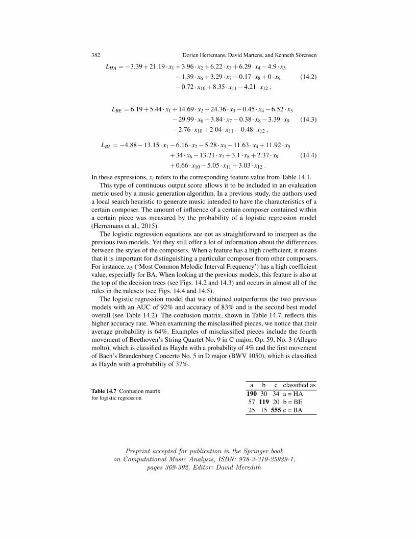
LHA =−3.39+21.19 · x1 +3.96 · x2 +6.22 · x3 +6.29 · x4−4.9 · x5

−1.39 · x6 +3.29 · x7−0.17 · x8 +0 · x9

−0.72 · x10 +8.35 · x11−4.21 · x12 ,

(14.2)

LBE = 6.19+5.44 · x1 +14.69 · x2 +24.36 · x3−0.45 · x4−6.52 · x5

−29.99 · x6 +3.84 · x7−0.38 · x8−3.39 · x9

−2.76 · x10 +2.04 · x11−0.48 · x12 ,

(14.3)

LBA =−4.88−13.15 · x1−6.16 · x2−5.28 · x3−11.63 · x4 +11.92 · x5

+34 · x6−13.21 · x7 +3.1 · x8 +2.37 · x9

+0.66 · x10−5.05 · x11 +3.03 · x12 .

(14.4)

In these expressions, xi refers to the corresponding feature value from Table 14.1.This type of continuous output score allows it to be included in an evaluation

metric used by a music generation algorithm. In a previous study, the authors useda local search heuristic to generate music intended to have the characteristics of acertain composer. The amount of influence of a certain composer contained withina certain piece was measured by the probability of a logistic regression model(Herremans et al., 2015).

The logistic regression equations are not as straightforward to interpret as theprevious two models. Yet they still offer a lot of information about the differencesbetween the styles of the composers. When a feature has a high coefficient, it meansthat it is important for distinguishing a particular composer from other composers.For instance, x5 (‘Most Common Melodic Interval Frequency’) has a high coefficientvalue, especially for BA. When looking at the previous models, this feature is also atthe top of the decision trees (see Figs. 14.2 and 14.3) and occurs in almost all of therules in the rulesets (see Figs. 14.4 and 14.5).

The logistic regression model that we obtained outperforms the two previousmodels with an AUC of 92% and accuracy of 83% and is the second best modeloverall (see Table 14.2). The confusion matrix, shown in Table 14.7, reflects thishigher accuracy rate. When examining the misclassified pieces, we notice that theiraverage probability is 64%. Examples of misclassified pieces include the fourthmovement of Beethoven’s String Quartet No. 9 in C major, Op. 59, No. 3 (Allegromolto), which is classified as Haydn with a probability of 4% and the first movementof Bach’s Brandenburg Concerto No. 5 in D major (BWV 1050), which is classifiedas Haydn with a probability of 37%.

Table 14.7 Confusion matrixfor logistic regression





14.4.4 Naive Bayes

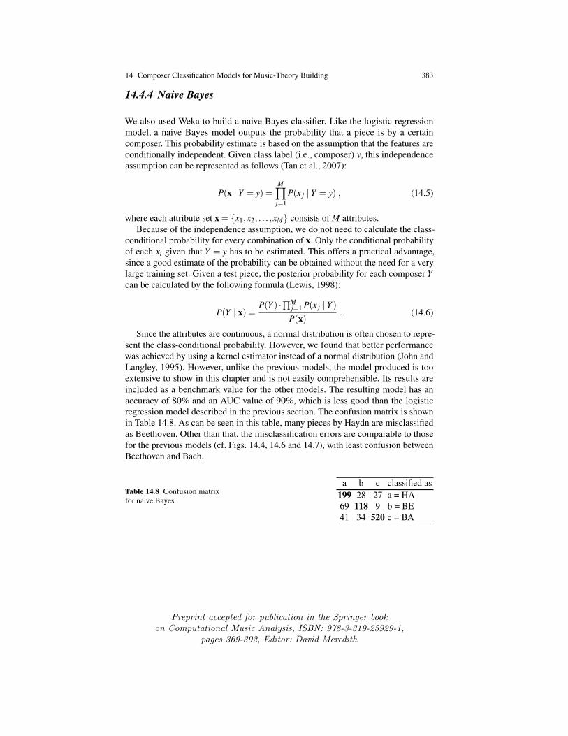
We also used Weka to build a naive Bayes classifier. Like the logistic regressionmodel, a naive Bayes model outputs the probability that a piece is by a certaincomposer. This probability estimate is based on the assumption that the features areconditionally independent. Given class label (i.e., composer) y, this independenceassumption can be represented as follows (Tan et al., 2007):

P(x | Y = y) =M

∏j=1

P(x j | Y = y) , (14.5)

where each attribute set x = {x1,x2, . . . ,xM} consists of M attributes.Because of the independence assumption, we do not need to calculate the class-

conditional probability for every combination of x. Only the conditional probabilityof each xi given that Y = y has to be estimated. This offers a practical advantage,since a good estimate of the probability can be obtained without the need for a verylarge training set. Given a test piece, the posterior probability for each composer Ycan be calculated by the following formula (Lewis, 1998):

P(Y | x) =P(Y ) ·∏M

j=1 P(x j | Y )P(x)

. (14.6)

Since the attributes are continuous, a normal distribution is often chosen to repre-sent the class-conditional probability. However, we found that better performancewas achieved by using a kernel estimator instead of a normal distribution (John andLangley, 1995). However, unlike the previous models, the model produced is tooextensive to show in this chapter and is not easily comprehensible. Its results areincluded as a benchmark value for the other models. The resulting model has anaccuracy of 80% and an AUC value of 90%, which is less good than the logisticregression model described in the previous section. The confusion matrix is shownin Table 14.8. As can be seen in this table, many pieces by Haydn are misclassifiedas Beethoven. Other than that, the misclassification errors are comparable to thosefor the previous models (cf. Figs. 14.4, 14.6 and 14.7), with least confusion betweenBeethoven and Bach.

Table 14.8 Confusion matrixfor naive Bayes





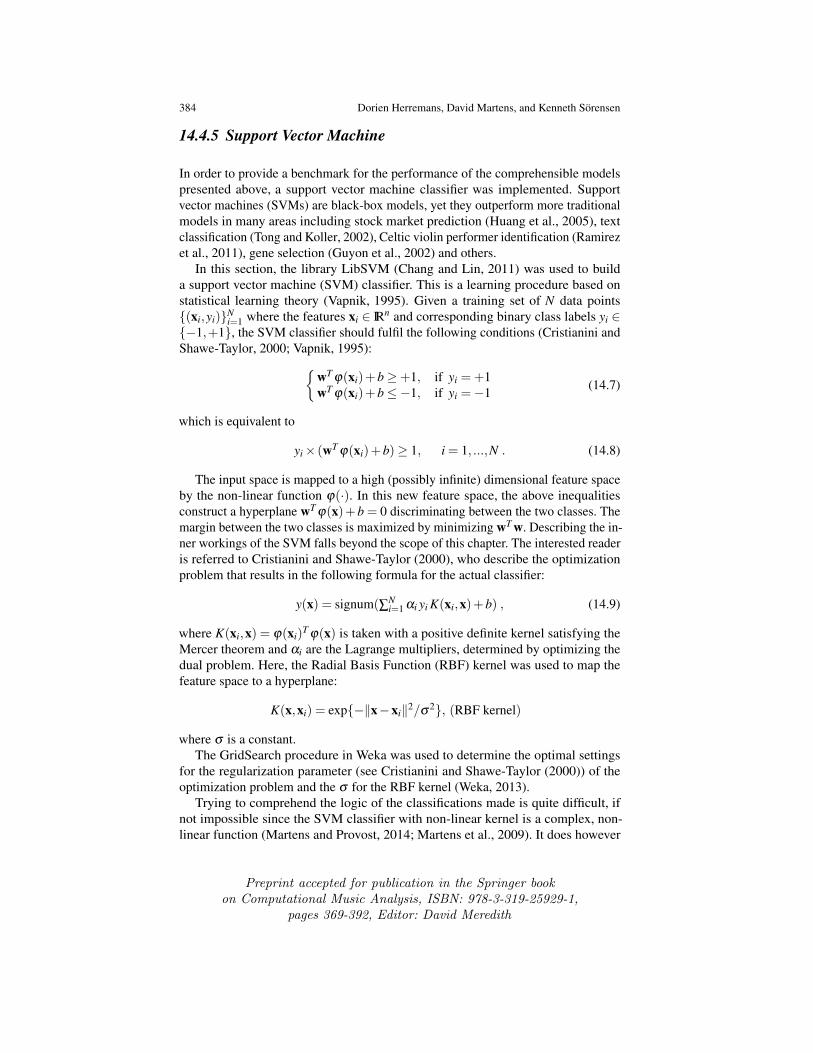
14.4.5 Support Vector Machine

In order to provide a benchmark for the performance of the comprehensible modelspresented above, a support vector machine classifier was implemented. Supportvector machines (SVMs) are black-box models, yet they outperform more traditionalmodels in many areas including stock market prediction (Huang et al., 2005), textclassification (Tong and Koller, 2002), Celtic violin performer identification (Ramirezet al., 2011), gene selection (Guyon et al., 2002) and others.

In this section, the library LibSVM (Chang and Lin, 2011) was used to builda support vector machine (SVM) classifier. This is a learning procedure based onstatistical learning theory (Vapnik, 1995). Given a training set of N data points{(xi,yi)}N

i=1 where the features xi ∈ IRn and corresponding binary class labels yi ∈{−1,+1}, the SVM classifier should fulfil the following conditions (Cristianini andShawe-Taylor, 2000; Vapnik, 1995):{

wT ϕ(xi)+b≥+1, if yi =+1wT ϕ(xi)+b≤−1, if yi =−1 (14.7)

which is equivalent to

yi× (wT ϕ(xi)+b)≥ 1, i = 1, ...,N . (14.8)

The input space is mapped to a high (possibly infinite) dimensional feature spaceby the non-linear function ϕ(·). In this new feature space, the above inequalitiesconstruct a hyperplane wT ϕ(x)+b = 0 discriminating between the two classes. Themargin between the two classes is maximized by minimizing wT w. Describing the in-ner workings of the SVM falls beyond the scope of this chapter. The interested readeris referred to Cristianini and Shawe-Taylor (2000), who describe the optimizationproblem that results in the following formula for the actual classifier:

y(x) = signum(∑Ni=1 αi yi K(xi,x)+b) , (14.9)

where K(xi,x) = ϕ(xi)T ϕ(x) is taken with a positive definite kernel satisfying the

Mercer theorem and αi are the Lagrange multipliers, determined by optimizing thedual problem. Here, the Radial Basis Function (RBF) kernel was used to map thefeature space to a hyperplane:

K(x,xi) = exp{−‖x−xi‖2/σ2}, (RBF kernel)

where σ is a constant.The GridSearch procedure in Weka was used to determine the optimal settings

for the regularization parameter (see Cristianini and Shawe-Taylor (2000)) of theoptimization problem and the σ for the RBF kernel (Weka, 2013).

Trying to comprehend the logic of the classifications made is quite difficult, ifnot impossible since the SVM classifier with non-linear kernel is a complex, non-linear function (Martens and Provost, 2014; Martens et al., 2009). It does however




Table 14.9 Confusion matrixfor support vector machines


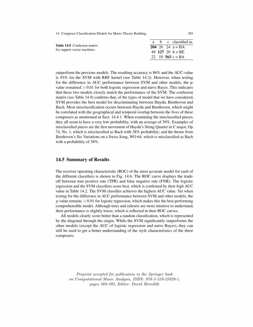
outperform the previous models. The resulting accuracy is 86% and the AUC-valueis 93% for the SVM with RBF kernel (see Table 14.2). However, when testingfor the difference in AUC performance between SVM and other models, the p-value remained > 0.01 for both logistic regression and naive Bayes. This indicatesthat these two models closely match the performance of the SVM. The confusionmatrix (see Table 14.9) confirms that, of the types of model that we have considered,SVM provides the best model for discriminating between Haydn, Beethoven andBach. Most misclassification occurs between Haydn and Beethoven, which mightbe correlated with the geographical and temporal overlap between the lives of thesecomposers as mentioned in Sect. 14.4.1. When examining the misclassified pieces,they all seem to have a very low probability, with an average of 39%. Examples ofmisclassified pieces are the first movement of Haydn’s String Quartet in C major, Op.74, No. 1, which is misclassified as Bach with 38% probability; and the theme fromBeethoven’s Six Variations on a Swiss Song, WO 64, which is misclassified as Bachwith a probability of 38%.

14.5 Summary of Results

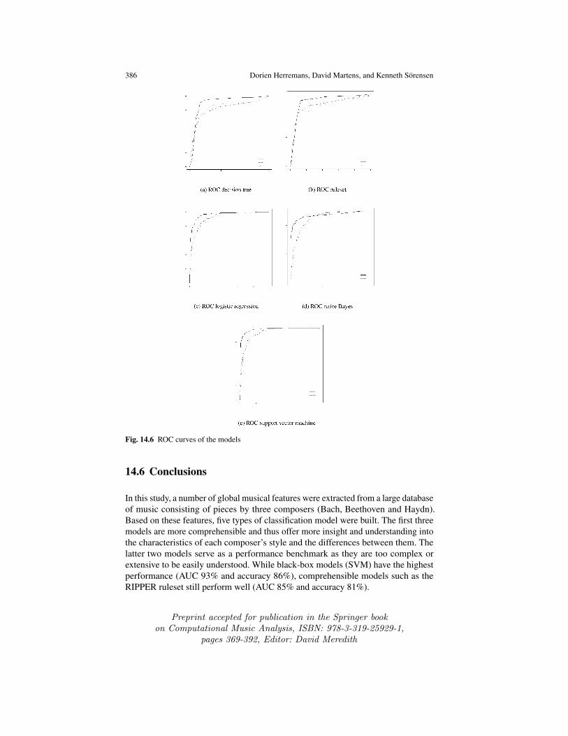
The receiver operating characteristic (ROC) of the most accurate model for each ofthe different classifiers is shown in Fig. 14.6. The ROC curve displays the trade-off between true positive rate (TPR) and false negative rate (FNR). The logisticregression and the SVM classifiers score best, which is confirmed by their high AUCvalue in Table 14.2. The SVM classifier achieves the highest AUC value. Yet whentesting for the difference in AUC performance between SVM and other models, thep-value remains > 0.01 for logistic regression, which makes this the best-performingcomprehensible model. Although trees and rulesets are more intuitive to understand,their performance is slightly lower, which is reflected in their ROC curves.

All models clearly score better than a random classification, which is representedby the diagonal through the origin. While the SVM significantly outperforms theother models (except the AUC of logistic regression and naive Bayes), they canstill be used to get a better understanding of the style characteristics of the threecomposers.




Fig. 14.6 ROC curves of the models

14.6 Conclusions

In this study, a number of global musical features were extracted from a large databaseof music consisting of pieces by three composers (Bach, Beethoven and Haydn).Based on these features, five types of classification model were built. The first threemodels are more comprehensible and thus offer more insight and understanding intothe characteristics of each composer’s style and the differences between them. Thelatter two models serve as a performance benchmark as they are too complex orextensive to be easily understood. While black-box models (SVM) have the highestperformance (AUC 93% and accuracy 86%), comprehensible models such as theRIPPER ruleset still perform well (AUC 85% and accuracy 81%).




The comprehensible models give us musical insights and can suggest directionsfor further musicological research. For example, the results of this study suggest thatBeethoven typically does not focus on using one particular interval, in contrast toHaydn or Bach, who have a higher prevalence of the most common melodic interval.Clearly, this result is based on a limited corpus and cannot be generalized withoutfurther investigation.

It would be interesting to examine whether an approach based on local featurescould contribute to gaining even more insight into the styles of composers. Classifi-cation models with an even higher accuracy rate might also be developed. It could beinteresting to extract comprehensible rules from SVM models with rule extractiontechniques such as Trepan and G-REX (Martens et al., 2007). This might providemore accurate comprehensible models. According to Backer and van Kranenburg(2005), the composers examined in the study reported in this chapter are relativelyeasy to distinguish. It would therefore be interesting to apply the methods from thischapter to distinguishing between composers whose styles are more similar, such asBach, Telemann and Handel.

References

Backer, E. and van Kranenburg, P. (2005). On musical stylometry—a pattern recog-nition approach. Pattern Recognition Letters, 26(3):299–309.

Berenzweig, A., Logan, B., Ellis, D., and Whitman, B. (2004). A large-scale eval-uation of acoustic and subjective music-similarity measures. Computer MusicJournal, 28(2):63–76.

Bohak, C. and Marolt, M. (2009). Calculating similarity of folk song variants withmelody-based features. In Proceedings of the 10th International Society for MusicInformation Retrieval Conference (ISMIR), pages 597–602, Kobe, Japan.

Casey, M., Veltkamp, R., Goto, M., Leman, M., Rhodes, C., and Slaney, M. (2008).Content-based music information retrieval: Current directions and future chal-lenges. Proceedings of the IEEE, 96(4):668–696.

CCARH (2012). KernScores, http://kern.ccarh.org. Last accessed: November 2012.Chang, C.-C. and Lin, C.-J. (2011). LIBSVM: A library for support vector machines.

ACM Transactions on Intelligent Systems and Technology (TIST), 2(3):27.Chew, E., Volk, A., and Lee, C.-Y. (2005). Dance music classification using inner

metric analysis. In Golden, B. L., Raghaven, S., and Wasil, E. A., editors, The NextWave in Computing, Optimization, and Decision Technologies, pages 355–370.Springer.

Cohen, W. (1995). Fast effective rule induction. In Proceedings of the 12th Interna-tional Conference on Machine Learning, pages 115–123, Tahoe City, CA.

Conklin, D. and Witten, I. H. (1995). Multiple viewpoint systems for music prediction.Journal of New Music Research, 24(1):51–73.




Cosi, P., De Poli, G., and Lauzzana, G. (1994). Auditory modelling and self-organizing neural networks for timbre classification. Journal of New MusicResearch, 23(1):71–98.

Cristianini, N. and Shawe-Taylor, J. (2000). An Introduction to Support VectorMachines and Other Kernel-Based Learning Methods. Cambridge UniversityPress.

DeNora, T. (1997). Beethoven and the Construction of Genius: Musical Politics inVienna, 1792-1803. University of California Press.

Downie, J. (2003). Music information retrieval. Annual Review of InformationScience and Technology, 37(1):295–340.

Eerola, T., Jarvinen, T., Louhivuori, J., and Toiviainen, P. (2001). Statistical featuresand perceived similarity of folk melodies. Music Perception, 18(3):275–296.

Eerola, T. and Toiviainen, P. (2004). MIR in Matlab: The Midi Toolbox. In Proceed-ings of 6th International Conference on Music Information Retrieval (ISMIR 2005),pages 22–27, London, UK.

Fawcett, T. (2004). ROC graphs: Notes and practical considerations for data miningresearchers. Technical Report HPL-2003-4, HP Laboratories, Palo Alto, CA.

Friedman, J., Hastie, T., and Tibshirani, R. (2000). Additive logistic regression: Astatistical view of boosting (with discussion and a rejoinder by the authors). TheAnnals Of Statistics, 28(2):337–407.

Geertzen, J. and van Zaanen, M. (2008). Composer classification using grammaticalinference. In Proceedings of the International Workshop on Machine Learningand Music (MML 2008), pages 17–18, Helsinki, Finland.

Gheyas, I. and Smith, L. (2010). Feature subset selection in large dimensionalitydomains. Pattern Recognition, 43(1):5–13.

Ghias, A., Logan, J., Chamberlin, D., and Smith, B. (1995). Query by humming:Musical information retrieval in an audio database. In Proceedings of the ThirdACM International Conference on Multimedia, pages 231–236, San Francisco,CA.

Greene, D. (1985). Greene’s Biographical Encyclopedia of Composers. The Repro-ducing Piano Roll Foundation. Edited by Alberg M. Petrak.

Guyon, I., Weston, J., Barnhill, S., and Vapnik, V. (2002). Gene selection for cancerclassification using support vector machines. Machine Learning, 46(1-3):389–422.

Hall, M., Frank, E., Holmes, G., Pfahringer, B., Reutemann, P., and Witten, I. (2009).The Weka data mining software: An update. ACM SIGKDD Explorations Newslet-ter, 11(1):10–18.

Herlands, W., Der, R., Greenberg, Y., and Levin, S. (2014). A machine learning ap-proach to musically meaningful homogeneous style classification. In Proceedingsof the 28th AAAI Conference on Artificial Intelligence (AAAI-14), pages 276–282,Quebec, Canada.

Herremans, D., Martens, D., and Sorensen, K. (2014). Dance hit song prediction.Journal of New Music Research, 43(3):291–302.

Herremans, D., Sorensen, K., and Martens, D. (2015). Classification and generationof composer-specific music using global feature models and variable neighborhoodsearch. Computer Music Journal, 39(3). In press.




Hillewaere, R., Manderick, B., and Conklin, D. (2009). Global feature versus eventmodels for folk song classification. In Proceedings of the 10th InternationalSociety for Music Information Retrieval Conference (ISMIR 2009), Kobe, Japan.

Hillewaere, R., Manderick, B., and Conklin, D. (2010). String quartet classificationwith monophonic models. In Proceedings of the 11th International Society forMusic Information Retrieval Conference (ISMIR 2010), Utrecht, The Netherlands.

Hillewaere, R., Manderick, B., and Conklin, D. (2012). String methods for folk tunegenre classification. In Proceedings of the 13th International Society for MusicInformation Retrieval Conference (ISMIR 2012), pages 217–222, Porto, Portugal.

Hontanilla, M., Perez-Sancho, C., and Inesta, J. (2013). Modeling musical style withlanguage models for composer recognition. In Sanchez, J. M., Mico, L., and Car-doso, J., editors, Pattern Recognition and Image Analysis: 6th Iberian Conference,IbPRIA 2013, Funchal, Madeira, Portugal, June 5–7. 2013, Proceedings, volume7887 of Lecture Notes in Computer Science, pages 740–748. Springer.

Huang, W., Nakamori, Y., and Wang, S.-Y. (2005). Forecasting stock market move-ment direction with support vector machine. Computers & Operations Research,32(10):2513–2522.

Huron, D. (2002). Music information processing using the Humdrum Toolkit:Concepts, examples, and lessons. Computer Music Journal, 26(2):11–26.

Jesser, B. (1991). Interaktive Melodieanalyse. Peter Lang.John, G. and Langley, P. (1995). Estimating continuous distributions in Bayesian

classifiers. In Proceedings of the Eleventh conference on Uncertainty in ArtificialIntelligence, pages 338–345, Montreal, Canada.

Kaliakatsos-Papakostas, M., Epitropakis, M., and Vrahatis, M. (2011). WeightedMarkov chain model for musical composer identification. In Chio, C. D., Cagnoni,S., Cotta, C., Ebner, M., and et al., A. E., editors, Applications of EvolutionaryComputation, volume 6625 of Lecture Notes in Computer Science, pages 334–343.Springer.

Kassler, M. (1966). Toward musical information retrieval. Perspectives of NewMusic, 4(2):59–67.

Landwehr, N., Hall, M., and Frank, E. (2005). Logistic model trees. MachineLearning, 59(1-2):161–205.

Laurier, C., Grivolla, J., and Herrera, P. (2008). Multimodal music mood classificationusing audio and lyrics. In Seventh International Conference on Machine Learningand Applications (ICMLA’08), pages 688–693, La Jolla, CA.

Lewis, D. (1998). Naive (Bayes) at forty: The independence assumption in in-formation retrieval. In Nedellec, C. and Rouveirol, C., editors, Machine Learn-ing: ECML-98, volume 1398 of Lecture Notes in Computer Science, pages 4–15.Springer.

Li, X., Ji, G., and Bilmes, J. (2006). A factored language model of quantized pitchand duration. In International Computer Music Conference (ICMC 2006), pages556–563, New Orleans, LA.

Mandel, M. and Ellis, D. (2005). Song-level features and support vector machinesfor music classification. In Proceedings of the 6th International Conference onMusic Information Retrieval (ISMIR 2006), pages 594–599, London, UK.




Martens, D. (2008). Building acceptable classification models for financial engineer-ing applications. SIGKDD Explorations, 10(2):30–31.

Martens, D., Baesens, B., Van Gestel, T., and Vanthienen, J. (2007). Comprehen-sible credit scoring models using rule extraction from support vector machines.European Journal of Operational Research, 183(3):1466–1476.

Martens, D. and Provost, F. (2014). Explaining data-driven document classifications.MIS Quarterly, 38(1):73–99.

Martens, D., Van Gestel, T., and Baesens, B. (2009). Decompositional rule extractionfrom support vector machines by active learning. IEEE Transactions on Knowledgeand Data Engineering, 21(2):178–191.

McKay, C. and Fujinaga, I. (2004). Automatic genre classification using large high-level musical feature sets. In Proceedings of the 5th International Conference onMusic Information Retrieval (ISMIR 2004), Barcelona, Spain.

McKay, C. and Fujinaga, I. (2006). jSymbolic: A feature extractor for MIDI files.In Proceedings of the International Computer Music Conference (ICMC 2006),pages 302–5, New Orleans, LA.

McKay, C. and Fujinaga, I. (2007). Style-independent computer-assisted exploratoryanalysis of large music collections. Journal of Interdisciplinary Music Studies,1(1):63–85.

McKay, C. and Fujinaga, I. (2008). Combining features extracted from audio, sym-bolic and cultural sources. In Proceedings of the 9th International Society forMusic Information Retrieval Conference (ISMIR 2008), pages 597–602, Philadel-phia, PA.

McKay, C. and Fujinaga, I. (2009). jMIR: Tools for automatic music classification.In Proceedings of the International Computer Music Conference (ICMC 2009),pages 65–8, Montreal, Canada.

Mearns, L., Tidhar, D., and Dixon, S. (2010). Characterisation of composer styleusing high-level musical features. In Proceedings of 3rd International Workshopon Machine Learning and Music, pages 37–40, Florence, Italy.

Mendel, A. (1969). Some preliminary attempts at computer-assisted style analysis inmusic. Computers and the Humanities, 4(1):41–52.

Moreno-Seco, F., Inesta, J., Ponce de Leon, P. J., and Mico, L. (2006). Comparison ofclassifier fusion methods for classification in pattern recognition tasks. In Yeung,D.-Y., Kwok, J. T., Roli, A. F. F., and de Ridder, D., editors, Structural, Syntactic,and Statistical Pattern Recognition: Joint IAPR International Workshops, SSPR2006 and SPR 2006, Hong Kong, China, August 17–19, 2006. Proceedings, volume4109 of LNCS, pages 705–713. Springer.

Pearce, M., Conklin, D., and Wiggins, G. (2005). Methods for combining statisticalmodels of music. In Kronland-Martinet, R., Voinier, T., and Ystad, S., editors,Computer Music Modeling and Retrieval, volume 3902 of LNCS, pages 295–312.Springer.

Perez-Sancho, C., Rizo, D., and Inesta, J. M. (2008). Stochastic text models for musiccategorization. In da Vitoria Lobo, N. and others, editors, Structural, Syntactic,and Statistical Pattern Recognition, volume 5342 of LNCS, pages 55–64. Springer.




Pfeiffer, S., Fischer, S., and Effelsberg, W. (1997). Automatic audio content analysis.In Proceedings of the 4th ACM International Conference on Multimedia, pages21–30, Boston, MA.

Pollastri, E. and Simoncelli, G. (2001). Classification of melodies by composer withhidden Markov models. In Web Delivering of Music, 2001. Proceedings. FirstInternational Conference on, pages 88–95. IEEE.

Ponce de Leon, P. J. and Inesta, J. (2003). Feature-driven recognition of music styles.In Perales, F. J., Campilho, A. J. C., de la Blanca, N. P., and Sanfeliu, A., editors,Pattern Recognition and Image Analysis: First Iberian Conference, IbPRIA 2003,Puerto de Andratx, Mallorca, Spain, volume 2652 of Lecture Notes in ComputerScience, pages 773–781. Springer.

Quinlan, J. (1993). C4.5: Programs for Machine Learning, volume 1. MorganKaufmann.

Ramirez, R., Maestre, E., Perez, A., and Serra, X. (2011). Automatic performeridentification in Celtic violin audio recordings. Journal of New Music Research,40(2):165–174.

Rosen, C. (1997). The Classical Style: Haydn, Mozart, Beethoven, volume 1. Norton.Ruggieri, S. (2002). Efficient C4. 5 [classification algorithm]. Knowledge and Data

Engineering, IEEE Transactions on, 14(2):438–444.Sapp, C. (2005). Online database of scores in the Humdrum file format. In Pro-

ceedings of the 6th International Conference on Music Information Retrieval(ISMIR 2005), pages 664–665, London, UK.

Shmueli, G. and Koppius, O. (2011). Predictive analytics in information systemsresearch. MIS Quarterly, 35(3):553–572.

Steinbeck, W. (1982). Struktur und Ahnlichkeit. In Methoden automatisierterMelodieanalyse. Barenreiter.

Stenzel, U. Lima, M. and Downes, J. . (2012). Study on Digital Content Products inthe EU, Framework contract: Evaluation impact assessment and related services;Lot 2: Consumer’s Policy. Technical report, EU, Brussels.

Tan, P. et al. (2007). Introduction to Data Mining. Pearson Education.Tong, S. and Koller, D. (2002). Support vector machine active learning with applica-

tions to text classification. The Journal of Machine Learning Research, 2:45–66.Tseng, Y.-H. (1999). Content-based retrieval for music collections. In Proceed-

ings of the 22nd Annual International ACM SIGIR Conference on Research andDevelopment in Information Retrieval, pages 176–182.

Tu, J. (1996). Advantages and disadvantages of using artificial neural networksversus logistic regression for predicting medical outcomes. Journal of ClinicalEpidemiology, 49(11):1225–1231.

Typke, R., Wiering, F., and Veltkamp, R. (2005). A survey of music informationretrieval systems. In Proceedings of the 6th International Conference on MusicInformation Retrieval (ISMIR 2005), pages 153–160, London, UK.

Tzanetakis, G. and Cook, P. (2002). Musical genre classification of audio signals.IEEE Transactions on Speech and Audio Processing, 10(5):293–302.




Tzanetakis, G., Ermolinskyi, A., and Cook, P. (2003). Pitch histograms in audio andsymbolic music information retrieval. Journal of New Music Research, 32(2):143–152.

van Kranenburg, P. (2008). On measuring musical style—The case of some disputedorgan fugues in the J. S. Bach (BWV) catalogue. Computing in Musicology,15:120–137.

van Kranenburg, P. (2010). A computational approach to content-based retrieval offolk song melodies. PhD thesis, Utrecht University.

van Kranenburg, P. and Backer, E. (2004). Musical style recognition—A quantitativeapproach. In Proceedings of the Conference on Interdisciplinary Musicology(CIM04), pages 106–107, Graz, Austria.

van Kranenburg, P., Volk, A., and Wiering, F. (2013). A comparison between globaland local features for computational classification of folk song melodies. Journalof New Music Research, 42(1):1–18.

Vapnik, V. (1995). The Nature of Statistical Learning Theory. Springer.Volk, A. and van Kranenburg, P. (2012). Melodic similarity among folk songs: An

annotation study on similarity-based categorization in music. Musicae Scientiae,16(3):317–339.

Weihs, C., Ligges, U., Morchen, F., and Mullensiefen, D. (2007). Classification inmusic research. Advances in Data Analysis and Classification, 1(3):255–291.

Weka (2013). Weka documentation, class GridSearch. Last accessed: October 2014.Whitman, B., Flake, G., and Lawrence, S. (2001). Artist detection in music with

Minnowmatch. In Neural Networks for Signal Processing XI, 2001. Proceedingsof the 2001 IEEE Signal Processing Society Workshop, pages 559–568. IEEE.

Whitman, B. and Smaragdis, P. (2002). Combining musical and cultural features forintelligent style detection. In Proceedings of the 3rd International Symposium onMusic Information Retrieval (ISMIR 2002), pages 47–52, Paris, France.

Witten, I. and Frank, E. (2005). Data Mining: Practical Machine Learning Toolsand Techniques. Morgan Kaufmann.

Wold, E., Blum, T., Keislar, D., and Wheaten, J. (1996). Content-based classification,search, and retrieval of audio. MultiMedia, IEEE, 3(3):27–36.

Wołkowicz, J., Kulka, Z., and Keselj, V. (2007). N-gram-based approach to composerrecognition. Master’s thesis, Warsaw University of Technology.

Wu, X., Kumar, V., Ross Quinlan, J., Ghosh, J., Yang, Q., Motoda, H., McLachlan, G.,Ng, A., Liu, B., Yu, P., et al. (2008). Top 10 algorithms in data mining. Knowledgeand Information Systems, 14(1):1–37.



Composer Classification Models for Music-Theory Building

Documents