Complexity and Entanglement for Pure and Mixed States in Quantum Field Theories Dissertation zur Erlangung des Grades eines Doktors der Naturwissenschaften am Fachbereich Physik der Freien Universit¨ at Berlin vorgelegt von Hugo Antonio Camargo Montero Berlin, August 2021

Welcome message from author
This document is posted to help you gain knowledge. Please leave a comment to let me know what you think about it! Share it to your friends and learn new things together.
Transcript
Complexity and Entanglement
for Pure and Mixed States in
Quantum Field Theories
Dissertation
zur Erlangung des Grades eines
Doktors der Naturwissenschaften
am
Fachbereich Physik
der
Freien Universitat Berlin
vorgelegt von
Hugo Antonio Camargo Montero
Berlin, August 2021

Betreuer Dr. Michal P. Heller
Hochschullehrer am Fachbereich Prof. Felix von Oppen, PhD
Zweitgutachter Prof. Dr. Jens Eisert
Datum der Disputation 6. Dezember 2021
Selbststandigkeitserklarung
Name: Camargo MonteroVorname: Hugo Antonio
Ich erklare gegenuber der Freien Universitat Berlin, dass ich die vorliegende Dis-sertation selbststandig und ohne Benutzung anderer als der angegebenen Quellenund Hilfsmittel angefertigt habe. Die vorliegende Arbeit ist frei von Plagiaten. AlleAusfuhrungen, die wortlich oder inhaltlich aus anderen Schriften entnommen sind,habe ich als solche kenntlich gemacht. Diese Dissertation wurde in gleicher oderahnlicher Form noch in keinem fruheren Promotionsverfahren eingereicht.
Mit einer Prufung meiner Arbeit durch ein Plagiatsprufungsprogramm erklare ichmich einverstanden.
Datum: 18.08.21 Unterschrift:

Abstract
Over the past two decades, ideas coming from quantum information science havesubstantially influenced the research carried out in the field of high-energy physics.This is particularly evident in the AdS/CFT correspondence, a framework whichpostulates a duality between certain gravitational theories on negatively-curved anti-de Sitter (AdS) spacetimes and conformal field theories (CFTs).
In this thesis we take a close look at quantities associated with two quantum in-formation theoretic notions which have led to novel insights into quantum gravitywithin the AdS/CFT correspondence: entanglement and complexity. Entanglemententropy (EE) is a well studied quantity that quantifies the pure state entanglementbetween a subregion and its complement, whose study has lead to outstanding res-ults in the field. Complexity, on the other hand, appeared recently in the context ofquantum field theories (QFTs) motivated by the aim of understanding the interior ofblack holes in the AdS/CFT and whose study in QFTs represents a very promisingresearch direction.
Particularly compelling open problems in our understanding of these quantities in-clude the time-dependence of complexity and the interplay between complexity andentanglement both in non-equilibrium systems and for subregions in QFTs cor-responding to mixed states. In this work we explore these problems in scenarioswhich allow us to make tractable computations and extract their universal proper-ties.
Within the former context, the study of quantum quenches is one of the most activeareas of research into non-equilibrium quantum dynamics. In this regard, we explorethe pure state complexity of exact time-dependent solutions for free scalar theoriesundergoing a quench through a critical point, finding evidence for universal scalingbehaviour dominated by the zero mode.
An intimately connected problem is the study of quantum information-theoreticproperties of mixed states in QFTs. In this context, we study complexity of puri-fication (CoP), entanglement of purification (EoP) and reflected entropy (RE). Forset-ups in free QFTs on a lattice which lead to Gaussian mixed states, we con-sider the most general Gaussian purifications and find universal properties using themathematical machinery of covariance matrices. In settings which lead to genuinelynon-Gaussian settings, we find a general proof valid for a CFT in any dimensionwith a gap in the operator spectrum, that EoP and RE exhibit an enhancementwith respect to the known power-law decay of mutual information measuring thecorrelations of a mixed state consisting of two subregions which are largely separ-ated. These result open a new avenue of research to study the properties of thesequantities from the perspective of CFT data.
Collectively, these findings set the stage to a better understanding of complexity andentanglement in QFTs by providing insights into their universal properties. Thisis paramount to elucidating the mechanism which connects gravity and quantumtheories within the AdS/CFT correspondence. Consequently, we believe that thesecan lead to a better understanding of quantum gravity and quite possibly to newtools in the study of quantum many-body systems.

Zusammenfassung
Ideen aus der Quanteninformation haben die Forschung auf dem Gebiet der Hochener-giephysik in den letzten zwei Jahrzehnten wesentlich beeinflusst. Dies zeigt sich insbesonderein der AdS/CFT-Korrespondenz, einer vorgeschlagenen Dualitat zwischen bestimmten Grav-itationstheorien auf negativ gekrummten Anti-De-Sitter (AdS)-Raumzeiten und konformenFeldtheorien (CFTs).
In dieser Arbeit studieren wir detailliert zwei Konzepte der Quanteninformation, welche zuneuen Einsichten in die Quantengravitation innerhalb der AdS/CFT-Korrespondenz gefuhrthaben: Verschrankung und Komplexitat. Die Verschrankungsentropie als eine bereits viel-fach untersuchte physikalische Große quantifiziert die Verschrankung reiner Zustande zwis-chen einem Teilgebiet und seinem Komplement. Ihre Untersuchung hat zu herausragendenErgebnissen auf diesem Gebiet gefuhrt. Andererseits tauchte Komplexitat erst kurzlich imKontext von Quantenfeldtheorien (QFTs) auf, motiviert durch das Ziel, das Innere vonSchwarzen Lochern mittels der AdS/CFT-Korrespondenz zu verstehen. Die damit einherge-henden Untersuchungen entwickeln sich zu einer sehr vielversprechenden neuen Forschung-srichtung.
Die Zeitabhangigkeit der Komplexitat und das Zusammenspiel zwischen Komplexitat undVerschrankung sowohl in Nicht-Gleichgewichtssystemen als auch in gemischten Zustandenin QFTs sind offene Probleme in unserem Verstandnis dieser Großen. In dieser Arbeit er-forschen wir diese Fragestellungen in Szenarien, die es uns erlauben, nachvollziehbare Berech-nungen durchzufuhren, um deren universelle Eigenschaften zu extrahieren.
Im ersteren Kontext ist das Studium von sogenannten Quantenquenchen eines der akt-ivsten Forschungsgebiete der Nicht-Gleichgewichts-Quantendynamik. Hier untersuchen wirdie reine Zustandskomplexitat von exakten zeitabhangigen Losungen fur freie Skalarthe-orien, die einen Quench durch einen kritischen Punkt durchlaufen. Wir finden Beweise furein universelles Skalierungsverhalten, das durch den Nullmodus dominiert wird.
Eine eng damit verbundene Problemstellung ist die Untersuchung der quanteninformations-theoretischen Eigenschaften von Mischzustanden in QFTs. In diesem Zusammenhang unter-suchen wir die sogenannte Komplexitat der Reinigung (CoP), die Verschrankung der Reini-gung (EoP) und die reflektierte Entropie (RE). Wir betrachten die allgemeinsten GaußschenReinigungen fur freie QFTs auf einem Gitter, die zu Gaußschen Mischzustanden fuhren, undfinden universelle Eigenschaften unter Verwendung mathematischer Methoden basierend aufKovarianzmatrizen. Fur echte nicht-Gaußsche Szenarien beweisen wir, dass EoP und REeine Verstarkung gegenuber dem bekannten Potenzgesetz-Abfall der sogenannten gegenseit-igen Information aufweisen, welche die Korrelationen gemischter Zustande misst, die auszwei weit voneinander entfernten Teilbereichen bestehen. Dieses Ergebnis gilt fur eine CFTin beliebiger Dimension mit einer Lucke im Operatorspektrum und eroffnet einen neuenForschungszweig, um die Eigenschaften dieser Großen aus der Perspektive von CFT-Datenzu untersuchen.
Zusammengenommen stellen diese Ergebnisse die Weichen fur ein besseres Verstandnis vonKomplexitat und Verschrankung in QFTs, indem sie Einblicke in deren universelle Ei-genschaften geben. Dies ist von entscheidender Bedeutung, um Aufschluss daruber zuerlangen, welche Mechanismen Gravitations- und Quantentheorien innerhalb der AdS/CFT-Korrespondenz miteinander verbinden. Folglich glauben wir, dass diese zu einem besserenVerstandnis der Quantengravitation und moglicherweise zu neuen methodischen Werkzeugenbei der Untersuchung von Quanten-Vielkorpersystemen fuhren konnen.

List of Contributions
This dissertation is based on the journal publications and preprint listed below.Chapter 4 is based on [CamH03]. Chapter 5 is based on [CamH02] and [CamH03].Chapter 6 is based on [CamH02] and [CamH01].
[CamH01] H. A. Camargo, L. Hackl, M. P. Heller, A. Jahn and B. Windt,“Long-distance entanglement of purification and reflected entropy in conformalfield theory”, arXiv:2102.00013 [hep-th] , Phys. Rev. Lett., vol. 127, p.141604, 2021, DOI: https://doi.org/10.1103/PhysRevLett.127.141604 . Note:
The preprint (arXiv) version of this publication, as published on arXiv, wasreviewed and approved by the Doctoral Thesis Committee.
My main contributions in this work involved performing numerical computationsfor entanglement of purification and reflected entropy as well as writing sectionsof the manuscript, producing figures and managing the journal submission.
[CamH02] H. A. Camargo, L. Hackl, M. P. Heller, A. Jahn, T. Takay-anagi and B. Windt, “Entanglement and Complexity of Purification in (1+1)-dimensional free Conformal Field Theories”, Phys. Rev. Res., vol. 3, p. 013248,2019, DOI: https://doi.org/10.1103/PhysRevResearch.3.013248 .
My main contributions in this work involved the initial formulation and earlydevelopment of the numerical algorithm used throughout this work and its im-plementation in the study of complexity of purification as well as writing sectionsof the manuscript, producing figures and managing the journal submission.
[CamH03] H. A. Camargo, P. Caputa, D. Das, M. P. Heller and R. Jef-ferson, “Complexity as a novel probe of quantum quenches: universal scalingsand purifications”, Phys. Rev. Lett. vol 122, no. 8, p. 081601, 2019, DOI: ht-tps://doi.org/10.1103/PhysRevLett.122.081601 .
My main contributions in this work involved performing analytical and numericalcomputations particularly in the context of complexity of purification as well aswriting the section of the appendix where details of this quantity are provided.
The following publications, not included in this thesis, were also produced duringthe course of doctoral research.
• H. A. Camargo, P. Caputa and P. Nandy, “Q-curvature and Path IntegralComplexity”, (2022), arXiv:2201.00562 [hep-th] .
• H. A. Camargo, M. P. Heller, R. Jefferson and J. Knaute, “Path integral op-timization as circuit complexity,”Phys. Rev. Lett., vol. 123, no. 1, p. 011601,2019, DOI: https://doi.org/10.1103/PhysRevLett.123.011601 .

Acknowledgments
I would like to begin by expressing my gratitude to my supervisor Michal P. Heller. Iwant to thank him for his patience, tireless support and scientific advice throughoutthese past four years. His commitment to hard work and passion for science arelessons that I will carry with me to the future. I am privileged to have been able togrow as scientist under his supervision.
I would also like to thank my fellow GQFI-ers, past and present, for many interestingphysics discussions, conversations, collaborations and advice. Thank you Nishan C J,Diptarka Das, Ro Jefferson, Eivind Jørstad, Johannes Knaute, Fernando Pastawski,Ignacio Reyes, Leo Shaposhnik, Sukhi Singh and Viktor Svensson. I am also gratefulto Jens Eisert for welcoming me into his group at FU and for our brief yet stimulatingphysics discussions.
My special gratitude also to my amazing collaborators throughout these years; PawelCaputa, Lucas Hackl, Alexander Jahn, Pratik Nandy, Tadashi Takayanagi and Ben-net Windt. I am thankful for the privilege of working with you and for all theinspiring discussions about physics that we had during the course of our collabora-tions.
I am indebted to the Konrad-Adenauer-Stiftung for giving me the opportunity tostudy in Germany. I would like to express my special gratitude to Simon Backovsky,Diego Cuadra, Maike Ender, Berthold Gees, Stefan Jost, Kerim Kudo and AndreaStudemann for their support and for allowing me to participate in many fascinatingseminars about Germany’s history, society and complex political reality.
I am also grateful to all the marvelous people that I met at the Max Planck In-stitute for Gravitational Physics (the Albert Einstein Institute). I would like tothank my friends at the AEI for all the great times throughout these years. AndreaAntonelli, Ana Alonso, Teresa Bautista, Enrico Brehm, Matteo Broccoli, LorenzoCasarin, Franz Ciceri, Roberto Cotesta, Alice Di Tucci, Shane Farnsworth, MarcoFinocchiaro, Jan Gerken, Serena Giardino, Hadi Godazgar, Alex Goeßmann, Car-oline Jonas, Isha Kotecha, Lars Kreutzer, Hannes Malcha, Matin Mojaza, AlejandroPenuela, Tung Tran, and Adriano Vigano. My special gratitude to Matthias Blit-tersdorf, Axel Kleinschmidt, Darya Niakhaichyk, Hermann Nicolai, Anika Rast andthe IT Department for all their kind help.
Being far away from home can be a challenging experience. I am grateful for myfamily and friends back home for their support throughout these past four years andspecially in recent times. I am especially thankful to my endless source of love, mymom. I would not have reached this point without her continuous encouragement.Finally, I am deeply grateful to Penelope for teaching me to smile again.

Contents
List of Contributions
1. Introduction 11.1. The Holographic Principle and the AdS/CFT Correspondence . . . . 4
1.1.1. The AdS/CFT Dictionary . . . . . . . . . . . . . . . . . . . . 81.2. Tensor Networks . . . . . . . . . . . . . . . . . . . . . . . . . . . . . 111.3. Organization of this thesis . . . . . . . . . . . . . . . . . . . . . . . . 16
2. Quantum Information Aspects of the AdS/CFT Correspondence 192.1. Holographic Entanglement Entropy . . . . . . . . . . . . . . . . . . . 19
2.1.1. The Ryu–Takayanagi Formula . . . . . . . . . . . . . . . . . 202.2. The Entanglement Wedge . . . . . . . . . . . . . . . . . . . . . . . . 23
2.2.1. The Entanglement Wedge Cross-Section . . . . . . . . . . . . 252.3. The Holographic Complexity Proposals . . . . . . . . . . . . . . . . 28
2.3.1. Actions and Volumes . . . . . . . . . . . . . . . . . . . . . . . 302.3.2. The Subregion Complexity Proposals . . . . . . . . . . . . . . 32
3. Complexity in Quantum Field Theory 373.1. Complexity in Quantum Information . . . . . . . . . . . . . . . . . . 37
3.1.1. The Geometric Approach to Circuit Complexity . . . . . . . 393.2. Gaussian Techniques . . . . . . . . . . . . . . . . . . . . . . . . . . . 41
3.2.1. The Covariance Matrix Approach . . . . . . . . . . . . . . . . 423.2.2. The Symplectic and Orthogonal Groups . . . . . . . . . . . . 443.2.3. The Relative Complex Structure and its Spectrum . . . . . . 45
3.3. Complexity in Quantum Field Theories . . . . . . . . . . . . . . . . 493.3.1. Complexity of the Klein–Gordon Vacuum . . . . . . . . . . . 503.3.2. Complexity of the Ising CFT Vacuum . . . . . . . . . . . . . 56
3.4. Discussion . . . . . . . . . . . . . . . . . . . . . . . . . . . . . . . . . 62
4. Complexity in Non-equilibrium Quantum Dynamics 654.1. Quenches in Quantum Field Theories . . . . . . . . . . . . . . . . . . 65
4.1.1. A Solvable Quench Model . . . . . . . . . . . . . . . . . . . . 674.2. The Universal Scalings of Complexity . . . . . . . . . . . . . . . . . 71
4.2.1. “Slow” Kibble–Zurek Regime . . . . . . . . . . . . . . . . . . 744.2.2. Fast Regime . . . . . . . . . . . . . . . . . . . . . . . . . . . . 77
4.3. Discussion . . . . . . . . . . . . . . . . . . . . . . . . . . . . . . . . . 78
5. Complexity of Purification 815.1. The Concept of Complexity of Purification . . . . . . . . . . . . . . 81
5.1.1. A Simple Model: Two Harmonic Oscillators . . . . . . . . . . 875.2. Vacuum Subregions of free Quantum Field Theories . . . . . . . . . 91
5.2.1. Fermionic Complexity of Purification . . . . . . . . . . . . . . 94
i
5.2.2. Bosonic Complexity of Purification . . . . . . . . . . . . . . . 955.2.3. Comparison of bosonic CoP with other methods . . . . . . . 97
5.3. Discussion . . . . . . . . . . . . . . . . . . . . . . . . . . . . . . . . . 102
6. Entanglement of Purification and Reflected Entropy 1056.1. The Concept of Entanglement of Purification and Reflected Entropy 105
6.1.1. The Concept of Entanglement of Purification . . . . . . . . . 1076.1.2. The Concept of Reflected Entropy . . . . . . . . . . . . . . . 108
6.2. Gaussian Entanglement of Purification . . . . . . . . . . . . . . . . . 1116.2.1. Adjacent Intervals in Free Conformal Field Theories . . . . . 1126.2.2. Small Separations in Free Bosonic CFTs . . . . . . . . . . . . 1146.2.3. Large Separations in Free Bosonic CFTs . . . . . . . . . . . . 1156.2.4. Universal Behaviour of Reflected Entropy in 2-dimensional
Conformal Field Theories . . . . . . . . . . . . . . . . . . . . 1166.3. Long Distance Behaviour in Free Conformal Field Theories . . . . . 116
6.3.1. General Argument . . . . . . . . . . . . . . . . . . . . . . . . 1176.3.2. MI, EoP and RE for Free Fermions and Ising Spins for Single
Site Intervals . . . . . . . . . . . . . . . . . . . . . . . . . . . 1216.4. Discussion . . . . . . . . . . . . . . . . . . . . . . . . . . . . . . . . . 123
7. Summary and Outlook 127
A. Appendices 133Appendices . . . . . . . . . . . . . . . . . . . . . . . . . . . . . . . . . . . 133A. Long-Distance Behaviour of MI, EoP and RE . . . . . . . . . . . . . 133
A.1. Free Fermions . . . . . . . . . . . . . . . . . . . . . . . . . . . 133A.2. Ising Spins . . . . . . . . . . . . . . . . . . . . . . . . . . . . 137
Bibliography 141
List of Figures
1.1. Diagram of the light-sheet constructed from the non-expanding lightrays emanating from a closed surface. . . . . . . . . . . . . . . . . . 6
1.2. Diagram of anti-de Sitter space and the bulk/boundary correspondence. 81.3. A multi-scale entanglement renormalization ansatz (MERA) tensor
network. . . . . . . . . . . . . . . . . . . . . . . . . . . . . . . . . . . 141.4. The MERA tensor network as a toy model of the AdS/CFT Corres-
pondence. . . . . . . . . . . . . . . . . . . . . . . . . . . . . . . . . . 15
2.1. Diagrams of a Ryu–Takayanagi surface in anti-de Sitter space. . . . 202.2. Diagram of RT surfaces in the bulk of a time-slice of an AdS3 Black
Hole. . . . . . . . . . . . . . . . . . . . . . . . . . . . . . . . . . . . . 212.3. Heuristic interpretation of the construction of the thermofield double
(TFD) state . . . . . . . . . . . . . . . . . . . . . . . . . . . . . . . . 242.4. Diagram of the entanglement wedge in anti-de Sitter space. . . . . . 252.5. Diagram of the entanglement wedge cross-section in anti-de Sitter space. 262.6. Representation of the time evolution of complexity in a strongly-
coupled system. . . . . . . . . . . . . . . . . . . . . . . . . . . . . . . 302.7. Diagrams of the holographic complexity proposals defined on an eternal
AdS black hole, dual to the thermofield-double (TFD) state. . . . . . 322.8. Diagrams of the holographic subregion complexity proposals. . . . . 34
3.1. An example of a quantum circuit. . . . . . . . . . . . . . . . . . . . . 383.2. Representation of the Jordan–Wigner transformation on a lattice. . . 58
4.1. Plot of the quench profile. . . . . . . . . . . . . . . . . . . . . . . . . 694.2. Plot of the time-dependence of complexity for different values of the
quench parameter. . . . . . . . . . . . . . . . . . . . . . . . . . . . . 744.3. Plot of complexity at the critical point as a function of the quench
parameter. . . . . . . . . . . . . . . . . . . . . . . . . . . . . . . . . . 754.4. Plot of single-mode contributions to complexity at the critical point as
a function of the quench parameter for different values of the angularwave number. . . . . . . . . . . . . . . . . . . . . . . . . . . . . . . . 76
4.5. Plot of the zero-mode contribution to complexity at the critical pointas a function of the quench parameter. . . . . . . . . . . . . . . . . . 77
5.1. Sketch of the geometric interpretation behind the complexity of puri-fication. . . . . . . . . . . . . . . . . . . . . . . . . . . . . . . . . . . 83
5.2. Comparison of the full complexity with complexity of purification fortwo harmonic oscillators. . . . . . . . . . . . . . . . . . . . . . . . . . 90
5.3. Sketch of the periodic lattice set-up used for the discretized (1 + 1)-dimensional Klein–Gordon and critical transverse Ising models. . . . 92
5.4. Fermionic complexity of purification for two adjacent subsystems. . . 95
iii
5.5. Bosonic complexity of purification for two adjacent subsystems inunits of the reference state frequency. . . . . . . . . . . . . . . . . . . 97
5.6. Comparison of the complexity of purification obtained using the fulloptimization algorithm and the approximate one obtained using thesingle-mode decomposition. . . . . . . . . . . . . . . . . . . . . . . . 100
5.7. Comparison of complexity of purification obtained using the Gaussianoptimization algorithm and the Fisher–Rao distance function for asingle interval and two adjacent intervals. . . . . . . . . . . . . . . . 101
6.1. Sketch of entanglement of purification and reflected entropy on aninfinite lattice. . . . . . . . . . . . . . . . . . . . . . . . . . . . . . . 110
6.2. Gaussian bosonic and fermionic entanglement of purification for ad-jacent subsystems. . . . . . . . . . . . . . . . . . . . . . . . . . . . . 113
6.3. Plots of the long-distance behaviour of mutual information, entangle-ment of purification and reflected entropy for free fermions and Isingspins. . . . . . . . . . . . . . . . . . . . . . . . . . . . . . . . . . . . 122
A.1. Visualization of the Jordan–Wigner transform in a one-dimensionallattice with subsystems consisting of two disjoint lattice sites. . . . . 134

List of Tables
6.1. Analytical and numerical results for the leading coefficient and theoffset for mutual information, entanglement of purification and reflec-ted entropy of vacuum subregions of the critical Ising model in termsof spins and free fermions. . . . . . . . . . . . . . . . . . . . . . . . . 121
v

1. Introduction
In the past ten years we have witnessed three historical events that stand out aslandmarks in humanity’s scientific enterprise. In 2012 the ATLAS and CMS ex-periments at the Large Hadron Collider (LHC) found experimental evidence for theexistence of the Higgs boson [1, 2]; a key ingredient of the Standard Model of particlephysics predicted over fifty years ago by Engler, Brout and Higgs [3, 4]. A few yearslater, the Laser Interferometer Gravitational-Wave Observatory (LIGO) detectedgravitational waves [5, 6]; originally predicted by Einstein himself over a hundredyears ago [7] and produced by the coalescence of compact binary objects such asblack holes. More recently, in 2019, the Event Horizon Telescope (EHT) collabora-tion obtained the first images of a black hole at the center of the Galaxy Messier 87(M87) [8], cementing our view that black holes are astrophysical objects that notonly exist as mathematical constructions and opening new avenues for studying theirastrophysical properties.
These unprecedented achievements are based on our two most successful physicaltheories to date: the Standard Model of particle physics, and Einstein’s generaltheory of relativity (GR). The former is based on quantum field theory (QFT) andis the framework with which we describe three of the fundamental interactions innature [9, 10]. The latter, on the other hand, is a geometric theory of the fundamentalinteraction between space, time and matter which has allowed us to tackle questionsabout gravity and the large-scale structure of the Universe [11–13].
Together, these theories make up the foundation of our most basic understanding ofnature. As a consequence, there exists a long-standing hope that these two distinctapproaches can be reconciled within a single framework. However, attempts to carryout this task have so far been either unsuccessful, or beyond our abilities to test them.Indeed, in certain cases these two theories even provide different and irreconcilablepredictions for the same phenomena and this fact is nowhere more evident than inthe study of black holes.
Classically, black holes are perfect traps in time and space from which nothing canescape. As astrophysical objects they represent the last stage of stellar evolutionand can even be found at galactic nuclei. From a mathematical perspective, thesefascinating objects were found to have mechanical properties which are analogous tothe laws of thermodynamics [14, 15]. Completing the thermodynamical picture ofblack holes was Hawking’s realisation that by taking into account quantum effectsnear the event horizon of a black hole, it could be shown that these objects infact produce radiation in a black-body-like fashion at a given temperature [16, 17],leading to their eventual and complete evaporation as they radiate their energyaway.
This inevitable evaporation of a black hole raises a profound question about the fateof the information contained in it once it completely evaporates. After all, a basic
1
CHAPTER 1. INTRODUCTION
principle of quantum mechanics is that the unitary evolution of a pure quantumstate into another one preserves the information contained therein. To put differ-ently, a pure state cannot evolve in time via a unitary operation into a mixed one,thereby losing information. As a consequence, an evident contradiction arises whenattempting to reconcile a black hole’s inevitable evaporation and the preservationof any in-falling information in the form of the unitary evolution of a quantumstate.
This so-called black hole information paradox, whose detailed explanation is beyondthe scope of this work, has stood as one of theoretical physics’ most puzzling openquestions for almost fifty years. Quite remarkably however, recent developmentsinvolving novel semi-classical computations [18, 19] have been used to reproduce thePage curve [20, 21], a necessary feature of unitary black hole evaporation, leading toa new phase in our understanding of the information paradox. See [22] for a reviewof such developments. Nevertheless, work remains to be done in order to claimits complete resolution. One can even argue that this would either require a moreprecise understanding of the quantum properties of gravity beyond semi-classicalapproaches [23, 24] or provide it.
At the same time, the black hole interior presents another outstanding puzzle. Inour classical understanding of black holes, nothing which travels through a blackhole horizon can ever get out. As a consequence, it is not possible to know whetherany unfortunate astronauts who attempt to take a closer look at a black hole willsmoothly traverse the horizon and continue to their inexorable death at a singularity,if they will instead violently combust at a firewall [25], or something completelydifferent all together.
Fortunately, over the past twenty years it has become increasingly clear that avery fruitful tool to tackle these and other pressing issues in our understanding ofgravity and its relation to the other fundamental interactions is to bring in quantuminformation science [26–28] into the equation.
Indeed a framework which has become the main stage for the convergence of ideascoming from different areas of physics is the anti-de Sitter/conformal field theory(AdS/CFT) correspondence [29–31]; a conjectured duality between certain quantumgravity and quantum field theories. Though arising from within the realm of stringtheory [32–37], over the past twenty years the correspondence has become a bridgebetween several disciplines ranging from condensed matter, to high-energy physicsand quantum information.
In particular, by looking at gravity through the lens of quantum information via theAdS/CFT correspondence, we are uncovering deep connections between spacetime,entanglement, tensor networks and quantum error correcting codes. The powerfuldual description of physical quantities enabled by the correspondence linking grav-ity and physics in negatively-curved spaces to quantum theory on a flat geometry isarguably the reason why it is one of the most active areas of research in theoreticalphysics, allowing us to tackle some of quantum gravity’s most challenging and press-ing issues while at the same time providing useful tools for understanding quantumsystems in regimes where it would otherwise be an insurmountable task.
2
In this thesis we take a close look at quantities associated with two quantum in-formation theoretic notions which have led to novel insights into quantum gravitywithin the AdS/CFT correspondence: entanglement and complexity. Entanglemententropy (EE) is a well studied quantity that quantifies the pure state entanglementbetween a subregion and its complement, whose study has lead to outstanding res-ults in the field. Complexity, on the other hand, appeared recently in the context ofquantum field theories (QFTs) motivated by the aim of understanding the interior ofblack holes in the AdS/CFT and whose study in QFTs represents a very promisingresearch direction.
Within the AdS/CFT correspondence, entanglement entropy (EE) and complexityacquire a geometric realization in terms of properties of certain hypersurfaces char-acterized by their codimension. This term refers to the complementary dimension ofgeometric objects and can be understood as follows: a hypersurface corresponding toa time-slice of a (D+1)-dimensional spacetime is be a codimension-1 object, while aregion such as the causal development of said time-slice D(Σt) is a codimension-0 ob-ject, regardless of the dimension (D+1) of the spacetime which contains them.
To be precise, holographic entanglement entropy (EE) acquires a natural geometricdescription as a generalization of the Bekenstein–Hawking entropy obtained fromthe area of codimension-2 surfaces in AdS and its connection to EE in CFTs hasalready been established for several years. Complexity, on the other hand, appearsas a conjectured realization of the observation that codimension-1 maximal volumesand codimension-0 causal developments which penetrate the event horizon of AdSblack holes have properties expected from the “difficulty” of preparing states inrandom quantum many-body systems.
Indeed a vast effort in the field has been devoted to understanding the propertiesof the holographic realization of complexity and to uncovering its field-theoreticproperties. The main reason being that understanding complexity within QFTspresents computational challenges surmounted by remaining within the field of freetheories or by exploiting the symmetries of CFTs, making a connection with itsholographic counterpart(s) beyond our reach for the moment.
At the same time, the quantum information-theoretic properties of mixed statescorresponding to spatial subregions in AdS are much less understood than their en-larged, pure-state counterparts. In particular, both the geometric and field-theoreticproperties of correlations between components of subregions and the complexity ofmixed states have not been completely understood despite their key roles within theAdS/CFT correspondence.
As a consequence, it is an essential task to improve our understanding of thesequantities both from the perspective of the AdS/CFT correspondence and of QFTs.Particularly compelling open problems in this direction include the time-dependenceof complexity and the interplay between complexity and entanglement both in non-equilibrium systems and for subregions in QFTs corresponding to mixed states. Inthis work we explore these problems in scenarios which allow us to make tractablecomputations and extract their universal properties in QFTs.
Within the former context, the study of quantum quenches is one of the most act-
3
CHAPTER 1. INTRODUCTION
ive areas of research into non-equilibrium quantum dynamics. In this regard, wewill explore the pure state complexity of exact time-dependent solutions for freescalar theories undergoing a quench through a critical point, with the goal of findingevidence for universal scalings. It has been proven, in fact, that EE exhibits uni-versal behaviour and it will be therefore interesting to contrast these findings withcomplexity.
In the context of quantum information-theoretic properties of mixed states, ourobjective will be to study mixed-state generalizations of pure state complexity andEE, as well as another interesting correlation measure in mixed states called reflectedentropy (RE). Our aim is to find properties of these quantities which are universalin CFTs and a natural stage for this exercise will be provided by lattice realizationsof said theories.
Collectively, our goal is to set the stage to a better understanding of complexity andentanglement in QFTs by providing insights into their universal properties. Thisis paramount to elucidating the mechanism which connects gravity and quantumtheories within the AdS/CFT correspondence. As argued above, this would lead toa better understanding of quantum gravity and quite possibly to new tools in thestudy of quantum many-body systems.
1.1. The Holographic Principle and the AdS/CFT Correspondence
The Anti-de Sitter/Conformal Field Theory (AdS/CFT) correspondence [38] is apowerful framework which posits an equivalence between two distinct physical the-ories; one which describes gravitational phenomena on an asymptotically anti-deSitter spacetime in D + 1 dimensions and another one which describes quantummany-body phenomena at theD-dimensional conformal boundary of said negatively-curved spacetime.
It is also a realization of the holographic principle [39–41]: a proposed tenet ofquantum gravity which roughly states that the physical information contained in aspacetime volume VD+1 can be thought of as encoded in its boundary (@V )D. Thename of the principle alludes to an analogy with optical holograms: the gravitationaltheory is the extra-dimensional image which emerges from the quantum theory livingon its lower-dimensional boundary. Originally discussed by ’t Hooft in the contextof black holes, this observation was elevated to the status of principle through ananalysis of entropy bounds for matter in gravitational systems.
The origin of the holographic principle dates back to the studies of black hole ther-modynamics and in particular to the statement that the entropy of a black hole isproportional to the area of its event horizon H via the Bekenstein–Hawking entropyformula
SBH =Area(H )
4GN, (1.1)
where GN is Newton’s constant [42]. This property of black holes is in contrast withother thermodynamical systems whose entropy scales with the volume enclosing thesystem rather than its area. Since one typically associates the number of degrees of
4
1.1. THE HOLOGRAPHIC PRINCIPLE AND THE ADS/CFTCORRESPONDENCE
freedom, or microstates, with the exponential of the entropy N eSBH , this suggeststhat the microstates describing a black hole with temperature TBH given by
TBH =
2, (1.2)
where is the event horizon’s surface gravity, are holographically encoded in its eventhorizon H . For example, for a Schwarzschild black hole of mass M the surfacegravity and area of the event horizon H are given respectively by = 1/4GNMand Area(H ) = 16G2
NM2 leading to a temperature and entropy given by TBH =1/(8GNM) and SBH = 4GNM2.
Following the generalized second law of black hole thermodynamics [43], Bekensteinargued that the entropy of in-falling matter into a black hole via a“Geroch process”, athought experiment proposed by Robert Geroch during a 1970 Princeton colloquiumin which a small thermodynamic system is moved from infinity into a black hole,must be bounded from above by
SMatter 2ER , (1.3)
where E is the energy of the in-falling matter contained in a sphere of radius R [44].This entropy bound was proven for quantum field theories in [45] based on thepositivity of relative entropy. Considering a matter system which instead of fallinginto a black hole collapses to form one, Susskind further argued [40] that the entropyof such a system is bounded by the area of the smallest sphere S that can containit
SMatter Area(S)
4GN. (1.4)
A drawback of Susskind’s spherical entropy bound (1.4) is that it is not generallyvalid in cosmological spacetimes. However, in 1999 Bousso [46] proposed a covariantgeneralization of it, formalized in terms of the area of the light-sheet L(B) of asurface B
S(L(B)) Area(B)
4GN, (1.5)
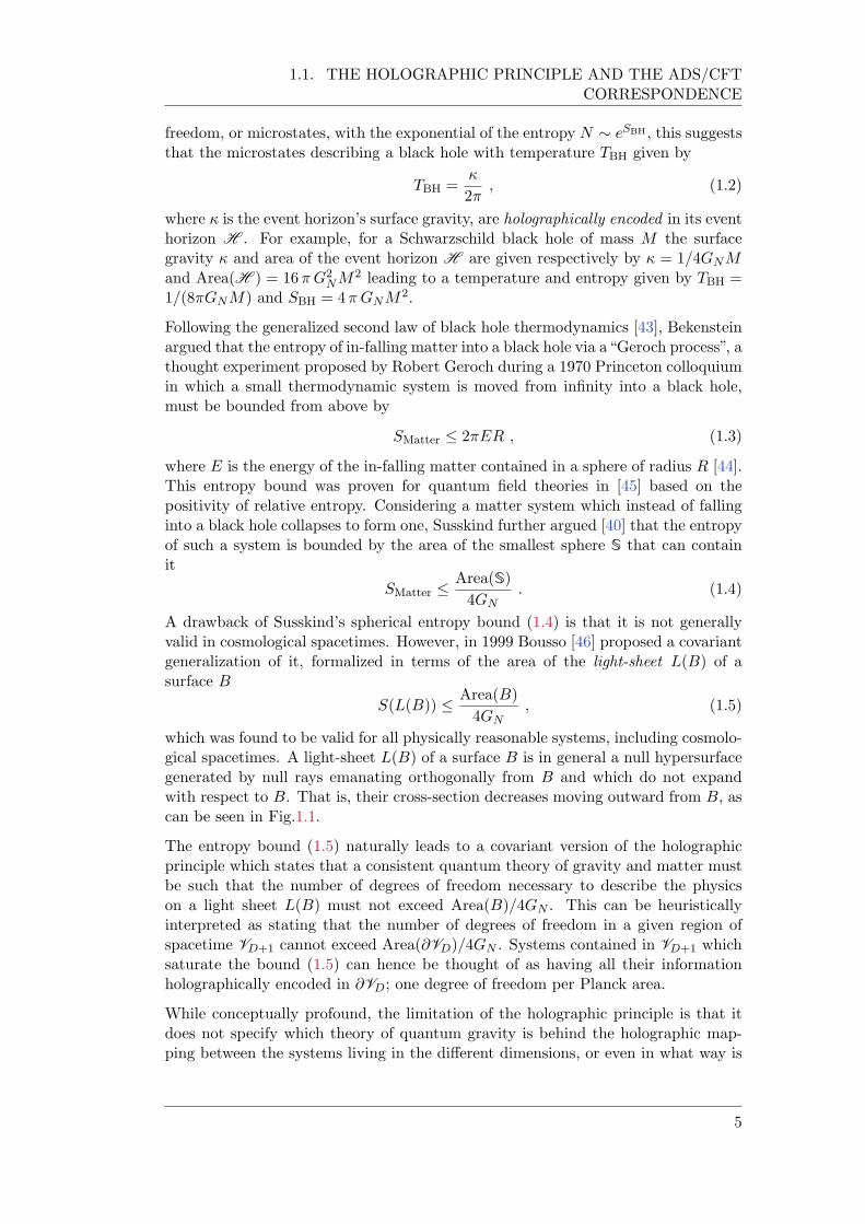
which was found to be valid for all physically reasonable systems, including cosmolo-gical spacetimes. A light-sheet L(B) of a surface B is in general a null hypersurfacegenerated by null rays emanating orthogonally from B and which do not expandwith respect to B. That is, their cross-section decreases moving outward from B, ascan be seen in Fig.1.1.
The entropy bound (1.5) naturally leads to a covariant version of the holographicprinciple which states that a consistent quantum theory of gravity and matter mustbe such that the number of degrees of freedom necessary to describe the physicson a light sheet L(B) must not exceed Area(B)/4GN . This can be heuristicallyinterpreted as stating that the number of degrees of freedom in a given region ofspacetime VD+1 cannot exceed Area(@VD)/4GN . Systems contained in VD+1 whichsaturate the bound (1.5) can hence be thought of as having all their informationholographically encoded in @VD; one degree of freedom per Planck area.
While conceptually profound, the limitation of the holographic principle is that itdoes not specify which theory of quantum gravity is behind the holographic map-ping between the systems living in the different dimensions, or even in what way is
5
CHAPTER 1. INTRODUCTION
Figure 1.1.: Diagram of the light-sheet L(B) constructed from the non-expandinglight rays emanating from a closed surface B. In this picture, the spher-ical surface B has four null hypersurfaces which are orthogonal to it.From these only two have a negative expansion and correspond to thefuture and past cones of the light-sheet L(B).
it implemented. This is why the AdS/CFT correspondence was not only rapidly em-braced by the community, but it was also met with an incredible amount of researchactivity: it provides a specific holographic mapping between two theories.
The most prominent example of the AdS/CFT correspondence is the dynamicalequivalence between N = 4 Super Yang–Mills (SYM) theory in (3 + 1)-dimensionalMinkoswki spacetime R
3,1 and type IIB superstring theory on AdS5 S5. Thisis in fact the original form of the conjecture and is sometimes also referred to asMaldacena’s AdS5/CFT4 correspondence.
N = 4 SYM is a non-Abelian gauge theory with gauge group SU(N) and Yang–Mills coupling constant gYM. It is also a maximally supersymmetric theory thatis also invariant under transformations of the conformal group SO(4, 2) and it ishence a conformal field theory (CFT). It corresponds to the “CFT” side of thecorrespondence.
Type IIB superstring theory, on the other hand, is a proposed quantum theory ofgravity characterized by two parameters; the string length ls =
p↵0 and the string
coupling gs. It is defined on the product spacetime AdS5S5, which involves anti-deSitter space of radius of curvature L and N units of Ramond-Ramond flux throughthe five-sphere S5. The dimensionless ratio L/
p↵0 and the coupling gs are the
independent parameters of the theory, which corresponds to the “AdS” side of thecorrespondence.
The free parameters on both sides of the correspondence are identified in the follow-ing way
g2YM = 2gs , 2g2YMN = L4/(↵0)2 . (1.6)
The second identification can be also be written in terms of the ‘t Hooft coupling := g2YMN as
=1
2
L
ls
4
. (1.7)
6
1.1. THE HOLOGRAPHIC PRINCIPLE AND THE ADS/CFTCORRESPONDENCE
The conjectured dynamical equivalence between these two theories implies that theydescribe the same physics from two different perspectives. The remarkable con-sequence of this is that we can describe a theory of quantum gravity, type IIBsuperstring theory, in terms of a gauge theory without any gravitational degrees offreedom, N = 4 SYM, and vice-versa. This interpretation of the correspondence isthe reason why it is also sometimes referred to as the gauge/gravity duality.
In its strongest form, the AdS5/CFT4 correspondence deals with arbitrary valuesof the dimension N of the gauge group SU(N) and the ‘t Hooft coupling , leadingto a full quantum description of the superstring theory on the gravitational side.However, since string theory is better understood perturbatively, one can considerthe weak string-coupling regime gs 1 while keeping the ratio L/ls constant. Atleading order in gs, this corresponds to classical string theory. On the CFT side,this leads to the large-N limit N ! 1 for fixed ; known as the ‘t Hooft limit.This is known as the strong form of Maldacena’s AdS5/CFT4 correspondence andis a realization of ‘t Hooft’s observation that a quantum field theory in the large-Nlimit has a perturbation series similar to that of a string theory in terms of planardiagrams [47].
In the limit where the string length ↵0 = l2s is taken to be small compared to theAdS radius L, i.e., ls/L ! 0, this equivalence leads to the strong/weak dualitybetween strongly-coupled N = 4 SYM with ! 1 and type IIB supergravityon weakly curved AdS5 S5. Hence in this regime classical gravity on a weaklynegatively-curved background is equivalent to a strongly-coupled quantum field the-ory. This is one of the main reasons why the AdS/CFT correspondence becamea very promising approach to study strongly-coupled quantum field theories, anotherwise monumental and in some cases even unfeasible task.
Indeed, one of the first successes of the correspondence was the computation ofthe ratio between the shear viscosity and the entropy density s of the deconfinedphase of N = 4 SYM [48] as a model for the quark-gluon plasma (QGP) of quantumchromodynamics (QCD). The expression for /s which was found to be universalin the ! 1 limit [49], is in remarkable semi-quantative agreement with estima-tions arising from experimental data obtained at the Relativistic Heavy Ion Collider(RHIC) laboratory in Brookhaven and the Large Hadron Collider (LHC) at CERN,where heavy-ion collisions are performed to study systems such as the QGP.
Nonetheless and as alluded to earlier in this section, the applicability of the Ad-S/CFT correspondence can be thought of as being broader than this particularexample. That is, other AdSD+1/CFTD correspondences can in principle be con-structed between different theories for different dimensions D. Indeed, even in Mal-dacena’s original work [38] other examples were proposed.
This observation is also consistent with the symmetries on both sides of the corres-pondence. AdSD+1 is a maximally symmetric (D + 1)-dimensional spacetime withsymmetry group SO(D, 2) which can be embedded in flat R
D,2 spacetime as a hy-perboloid. The symmetries of AdSD+1 precisely match the conformal and spacetimesymmetries of CFTD, also given by the conformal group SO(D, 2). A remarkableexample is the case of AdS3/CFT2 where it was found years prior to the original pro-posal, that the algebra of AdS3 generators turns into the SO(2, 2) conformal algebra
7
CHAPTER 1. INTRODUCTION
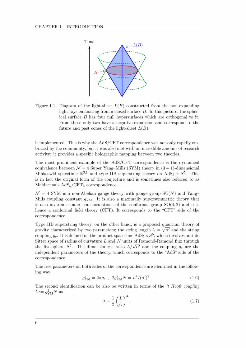
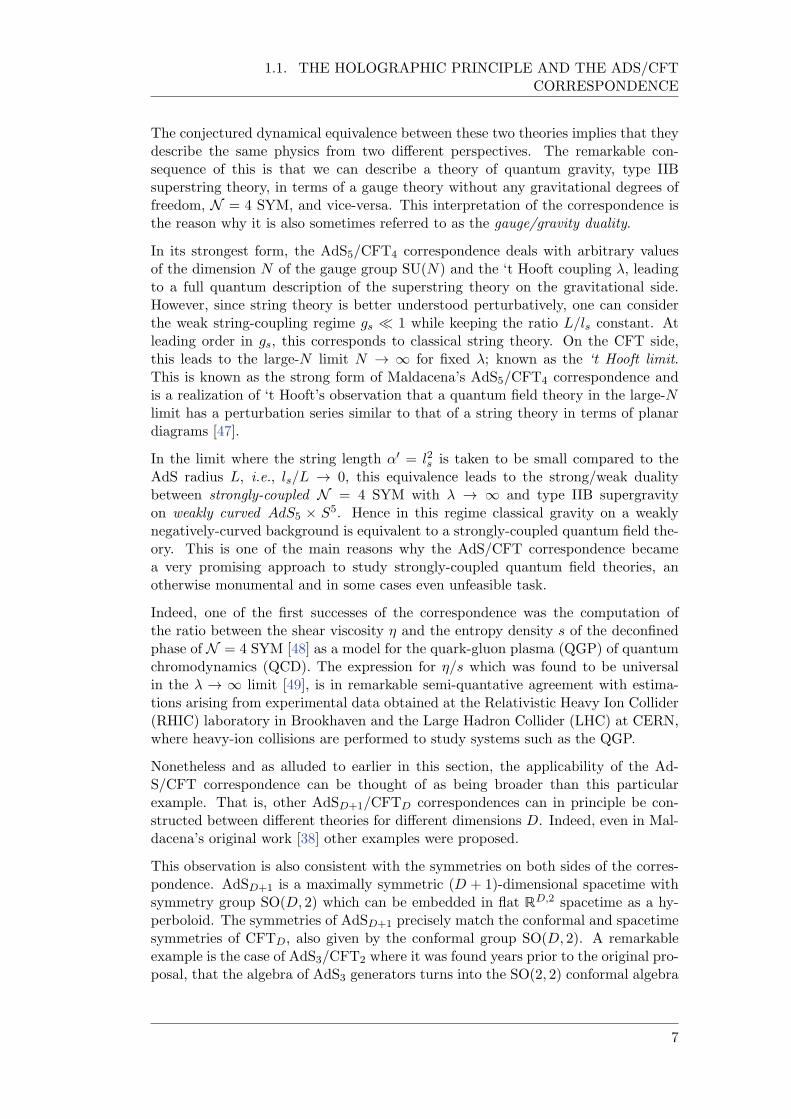
Figure 1.2.: Diagram of the bulk/boundary correspondence in AdS/CFT. TheAdSD+1 spacetime is represented by the interior (bulk) of the cylin-der, with its conformal boundary located represented by the boundaryof said cylinder. A time slice t =const of AdSD+1 is a negatively-curvedhyperbolic space. The pink shaded region corresponds to the Poincarepatch characterized by the metric (1.8).
at the conformal boundary of AdS3 [50].
Moreover, it can be seen that the supersymmetries of the field theory are relatedto the compact symmetries of the gravitational theory. In Maldacena’s AdS5/CFT4
case, the isometry group of S5 is SO(6), which coincides with part of the bosonicsubgroup of the supergroup of N = 4 SYM given by SU(4) SO(6). Together withthe spacetime symmetries discussed above, there is a full agreement between thesymmetries of both theories. A natural question, however, in this case is whethersupersymmetries are a necessary ingredient of the correspondence. Since these can beargued to be related to the compact dimensions in the case of AdS5S5, it is perhapsreasonable to suspect the validity of a non-supersymmetric type of duality.
1.1.1. The AdS/CFT Dictionary
The AdS/CFT correspondence is a duality between two theories. As such, it providesa one-to-one mapping between objects such as operators and fields on both sides.This mapping is collectively called the AdS/CFT dictionary.
The first entry in the dictionary is the identification of the flat background spacetimeR
D1,1 of the CFTD with the conformal boundary of the AdSD+1 spacetime, whichis consistent with the analysis of symmetries from the previous section. In thisregard, one often refers to the interior of the AdSD+1 spacetime as the bulk and tothe asymptotic R
D1,1 spacetime where the CFTD “lives”, as the boundary. Thiscan be seen in Fig. 1.2.
8
1.1. THE HOLOGRAPHIC PRINCIPLE AND THE ADS/CFTCORRESPONDENCE
To be precise, consider the Euclidean AdSD+1 spacetime whose metric in local Poin-care coordinates z, , ~x is given by
ds2 =L2
z2dz2 + d2 + d~x2
, (1.8)
which has constant negative curvature R = D(D+1)/L2 and satisfies the vacuumEinstein equations with cosmological constant Λ = D(D1)/(2L2). This coordin-ate system covers only a portion of global ADS called the Poincare patch. In thiscase, the conformal boundary of AdSD+1 is located at z = 0, while the Poincare ho-rizon is located at z !1. In Fig. 1.2, t is a global time coordinate while z extendsfrom the boundary of the cylinder towards its central axis bounded by the Poincarehorizon. Furthermore, in these coordinates, each z =const. slice corresponds to aflat RD1,1 spacetime.
The bulk/boundary mapping between the two theories relates objects on both sides,such as fields on the AdS side with operators O on the holographic CFT side. Itis based on the identification of partition functions Z on both sides of the corres-pondence
ZCFT[O] ZAdS[] , (1.9)
as proposed in the Gubser-Klebanov-Polyakov-Witten (GKPW) method [51, 52].To be precise, boundary configurations of sources, as encoded in the path-integrals,specify gravitational problems whose solution in semi-classical configurations providean approximation to the evaluation of the path-integral in the holographically dualCFT.
Consider, for example, a CFT operator O with scaling dimension∆, whose two-pointcorrelation function in the vacuum is
hO(~x)O(~y)i / 1
|~x ~y|2∆ , (1.10)
and where ~x and ~y are two points at the boundary. The GKPW method relates theboundary operator O with a dual field in the bulk, with boundary value (0), thatis
limz!0
(z,x) = z∆±(0)(x) := ±(x) , (1.11)
where the coefficient ∆+ ∆ leads to a so-called leading mode +, ∆ = D ∆
leads to a sub-leading mode and where ∆ coincides with the scaling dimensionof the CFT operator O dual to the field . Focusing on the sub-leading mode in thestandard quantisation allows us to compute the partition function (1.9) which takesthe form
ZAdS[]
φ(0)(x)=limz!0(z∆Dφ(z,x))
=
exp
ZdDx O (0)
CFT
, (1.12)
where one typically takes the saddle-point approximation on the left hand side.That is, the boundary value (0) of the field is interpreted as a source of thedual CFT operator O. This relation has been used, for example, to compute therelation between the mass m of a bulk scalar field and the scaling dimension ∆ of its
9
CHAPTER 1. INTRODUCTION
dual operator [52], showing how indeed the AdS/CFT dictionary provides a precisemapping between asymptotic bulk fields and boundary CFT operators.
Despite the fact that there is not a formal proof of the AdS/CFT correspondence,several entries of the AdS/CFT dictionary have been found both in the originalexample as well as in several others, providing evidence that the conjecture is correctand applicable in more general scenarios.1 Furthermore, Maldacena’s AdS5/CFT4
conjecture has been extremely well tested at the planar level using integrabilitytechniques (see e.g., [55–57] for some reviews). Such entries have applications rangingfrom high energy physics to condensed matter physics. Indeed, since the inception ofthe AdS/CFT correspondence there has been an extraordinary amount of exchangeof ideas between these disciplines which are reshaping the way we approach differentphenomena in various areas of physics. For a review of applications of AdS/CFT tocondensed matter physics see [30, 58–60]. Other resources for its applications to thestudy of QCD are [61–63]and we further refer the reader to the earlier discussion ofthe ratio /s of the deconfined phase of N = 4 SYM as a model for the QGP ofQCD.
Despite the successes of the AdS/CFT correspondence there are still outstandingquestions about the mechanism behind it. For example, how are the spacetimegeometry and other local gravitational observables encoded in a CFT state, or whatare the necessary and sufficient conditions for a QFT to have a dual gravitationaltheory.
However, over the past fifteen years it has become increasingly clear that a very usefulway to tackle these questions and other related ones, is to think about the CFT fromthe perspective of quantum information science. For example, a considerable amountof evidence has arisen which shows that the entanglement structure of CFT statesis directly related to the geometrical structure of the dual spacetime. Quantuminformation-theoretic quantities such as entanglement entropy and relative entropyhave been shown to have natural gravitational duals. At the same time, complexityhas emerged as a quantum information-theoretic quantity conjectured to encodeinformation about black hole interiors. This thesis deals with the field-theoreticproperties of mixed-state generalizations of these notions.
Further evidence for this intimate relation has also emerged from tensor networks(TN), a powerful computational tool used in quantum many-body systems, and alsofrom associated quantum error-correcting codes. In the following Section we give abrief review of the former, while a discussion of the latter is beyond the scope of thisthesis, but the reader can refer to [64, 65] for a review on the topic.
1While this claim is conjectured to hold between any CFT on R SD1 and a quantum theoryon gravity in asymptotically AdSD+1 M , where M is some compact manifold, in practice oneassumes that the gravitational dual of the CFT is a semicalssical theory of gravity described
by an effective action with a UV cutoff Λ such that 1/L Λ 1/G1
(D−1)
N . This implies inparticular that gapped large-N CFTs are expected have a semiclassical dual [53, 54].
10
1.2. TENSOR NETWORKS
1.2. Tensor Networks
Tensor network (TN) states are variational wavefunction ansatze for states in quantummany-body systems whose coefficients can be written as a contraction of “funda-mental” tensors which encode correlations between different subsystems. Their con-struction usually takes place within lattice models although some TNs have a con-tinuous counterpart. They are useful for representing ground states of local Hamilto-nians and they have also been used as toy models for holographic error-correctingcodes. See [66, 67] for recent reviews.
Consider a pure state |Ψi in a Hilbert space H with N degrees of freedom, whereeach one of them corresponds to an M -level system. That is, each degree of freedomcan take M different values. In a basis of H given by
|j1, . . . , jN i = |j1i . . . |jN i , (1.13)
we can represent the state |Ψi as
|Ψi =MX
j1,...,jN=1
Ψj1,...,jN |j1, . . . , jN i , (1.14)
where the MN coefficients Ψj1,...,jN 2 C define a complex-valued tensor Ψ of rank N .In general, the dimension of the indices ji is called the physical dimension j = M ,since it describes the dimension of local Hilbert spaces. The question which lies at thefoundation of TN is whether all the information encoded in the coefficients Ψj1,...,jN
is useful or needed to study specific properties of the state |Ψi.
Hence, the TN representation of |Ψi consists in writing the coefficients Ψj1,...,jN
as contractions of more fundamental tensors which accurately capture said correl-ations between different subsystems in H. For example, in the case N = 4 we canwrite
Ψj1,j2,j3,j4 =
χkX
k1,k2,k3,k4=1
Tj1,k4,k1Uj2,k1,k2Vj3,k2,k3Wj4,k3,k4 , (1.15)
where T, U, V,W, are tensors of rank 3 and where k is the bond dimension of the kindices.
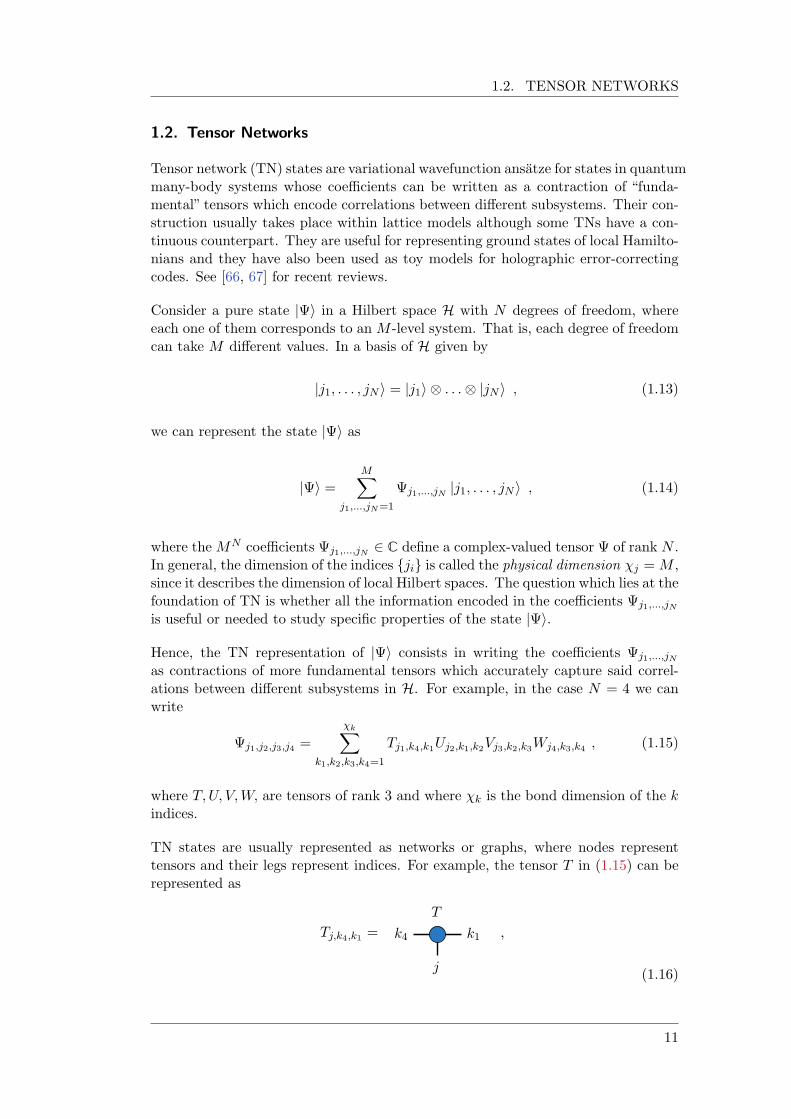
TN states are usually represented as networks or graphs, where nodes representtensors and their legs represent indices. For example, the tensor T in (1.15) can berepresented as
Tj,k4,k1 =
T
j
k4 k1 ,
(1.16)
11
CHAPTER 1. INTRODUCTION
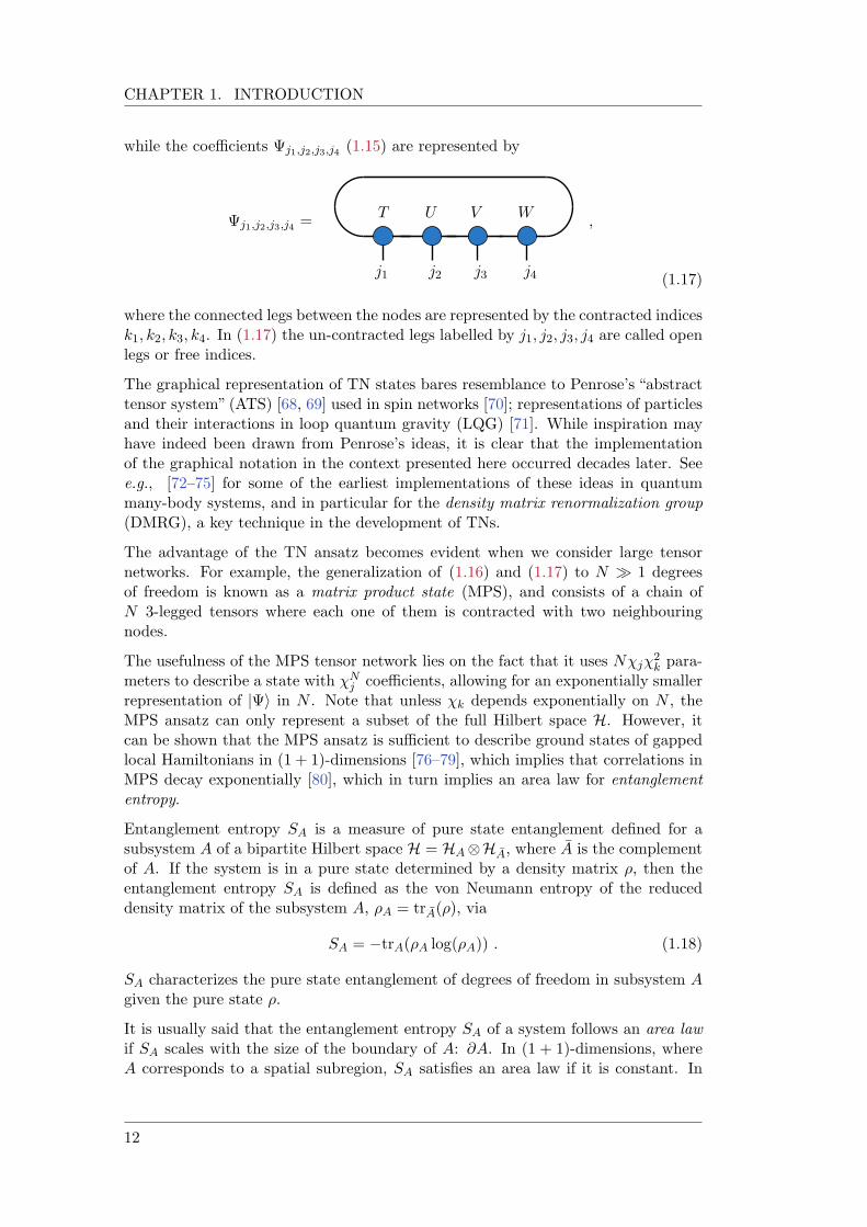
while the coefficients Ψj1,j2,j3,j4 (1.15) are represented by
Ψj1,j2,j3,j4 =T U V W
j1 j2 j3 j4
,
(1.17)
where the connected legs between the nodes are represented by the contracted indicesk1, k2, k3, k4. In (1.17) the un-contracted legs labelled by j1, j2, j3, j4 are called openlegs or free indices.
The graphical representation of TN states bares resemblance to Penrose’s “abstracttensor system” (ATS) [68, 69] used in spin networks [70]; representations of particlesand their interactions in loop quantum gravity (LQG) [71]. While inspiration mayhave indeed been drawn from Penrose’s ideas, it is clear that the implementationof the graphical notation in the context presented here occurred decades later. Seee.g., [72–75] for some of the earliest implementations of these ideas in quantummany-body systems, and in particular for the density matrix renormalization group(DMRG), a key technique in the development of TNs.
The advantage of the TN ansatz becomes evident when we consider large tensornetworks. For example, the generalization of (1.16) and (1.17) to N 1 degreesof freedom is known as a matrix product state (MPS), and consists of a chain ofN 3-legged tensors where each one of them is contracted with two neighbouringnodes.
The usefulness of the MPS tensor network lies on the fact that it uses Nj2k para-
meters to describe a state with Nj coefficients, allowing for an exponentially smaller
representation of |Ψi in N . Note that unless k depends exponentially on N , theMPS ansatz can only represent a subset of the full Hilbert space H. However, itcan be shown that the MPS ansatz is sufficient to describe ground states of gappedlocal Hamiltonians in (1 + 1)-dimensions [76–79], which implies that correlations inMPS decay exponentially [80], which in turn implies an area law for entanglemententropy.
Entanglement entropy SA is a measure of pure state entanglement defined for asubsystem A of a bipartite Hilbert space H = HAHA, where A is the complementof A. If the system is in a pure state determined by a density matrix , then theentanglement entropy SA is defined as the von Neumann entropy of the reduceddensity matrix of the subsystem A, A = trA(), via
SA = trA(A log(A)) . (1.18)
SA characterizes the pure state entanglement of degrees of freedom in subsystem Agiven the pure state .
It is usually said that the entanglement entropy SA of a system follows an area lawif SA scales with the size of the boundary of A: @A. In (1 + 1)-dimensions, whereA corresponds to a spatial subregion, SA satisfies an area law if it is constant. In
12
1.2. TENSOR NETWORKS
general, area laws are characteristic of ground states of gapped local Hamiltonians,and have been proven rigorously in (1 + 1)-dimensions [76] and for non-interactingsystems in arbitrary dimensions [81, 82]. For example, the entanglement entropyof connected subsystems in an MPS is constant in their size. See [83] for a review.We will discuss entanglement entropy and other correlation measures in detail inChapter 6 of this thesis.
For TN states of arbitrary geometry it can be shown that the entanglement entropySA of a subregion A is generally bounded from above as
SA |A| log(k) , (1.19)
where k is the bond dimension of all internal contracted legs in the network andwhere |A| is the length of the minimal cut A as counted by the number of legs itcuts; i.e., A is the line that divides the tensor network into two pieces correspondingtoA and A and which cuts through the smallest number of legs between tensors in thenetwork. This bound can be derived by a careful analysis of the Schmidt and singularvalue decompositions (SVD) of a bipartite quantum state. The entanglement entropySA will be maximal if all the Schmidt coefficients of the state are equal to thereciprocal of the bond dimension.
Not all TN represent states whose entanglement satisfies an area law. States thatarise from critical or gapless Hamiltonians, as in the case for conformal field theories(CFTs), have a more complicated entanglement structure. In (1 + 1)-dimensionalCFTs, the entanglement entropy SA of a subsystem A of size ` = |A| has a logar-ithmic scaling [84–86]
SA =c
3log
`
, (1.20)
where c is the central charge of the CFT and is a lattice (UV) regulator.
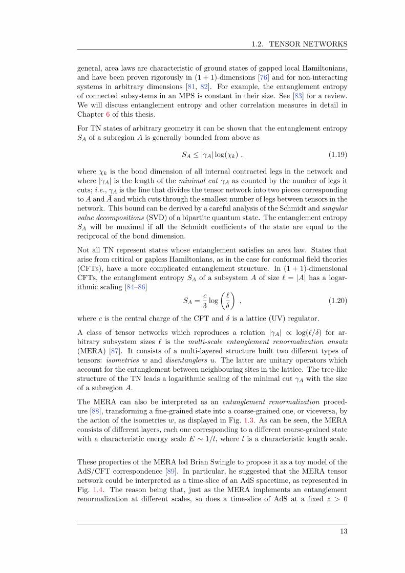
A class of tensor networks which reproduces a relation |A| / log(`/) for ar-bitrary subsystem sizes ` is the multi-scale entanglement renormalization ansatz(MERA) [87]. It consists of a multi-layered structure built two different types oftensors: isometries w and disentanglers u. The latter are unitary operators whichaccount for the entanglement between neighbouring sites in the lattice. The tree-likestructure of the TN leads a logarithmic scaling of the minimal cut A with the sizeof a subregion A.
The MERA can also be interpreted as an entanglement renormalization proced-ure [88], transforming a fine-grained state into a coarse-grained one, or viceversa, bythe action of the isometries w, as displayed in Fig. 1.3. As can be seen, the MERAconsists of different layers, each one corresponding to a different coarse-grained statewith a characteristic energy scale E 1/l, where l is a characteristic length scale.
These properties of the MERA led Brian Swingle to propose it as a toy model of theAdS/CFT correspondence [89]. In particular, he suggested that the MERA tensornetwork could be interpreted as a time-slice of an AdS spacetime, as represented inFig. 1.4. The reason being that, just as the MERA implements an entanglementrenormalization at different scales, so does a time-slice of AdS at a fixed z > 0
13
CHAPTER 1. INTRODUCTION
Figure 1.3.: A MERA tensor network composed of disentanglers u (squares) andisometries w (triangles). On the left, the entanglement renormalizationof MERA on lattice sites (circles) at various coarse-grained scales. Thevertical direction corresponds to the depth of the network, increasinglycoarse-graining the state as it moves upward. On the right, the identitiesof disentanglers and isometries for contractions with their Hermitianconjugates.
describes an increasingly coarse-grained state. Moreover, the critical states that areproduced by the MERA resemble those of conformal field theories.
However, the network geometry does not exactly match that of a time-slice ofAdS, leading to inconsistencies [90]. Alternative proposals have also interpreted theMERA network geometry as a path integral discretization of a null cone in AdS [91],as a time-like surface in de Sitter [92], and as a discretization of the kinematic spaceof AdS [93].
In [91], authors also proposed an extension of MERA which incorporates Euclideantime-evolution in (1 + 1)-dimensional CFTs through operators known as euclideonse, leading to a TN known as Euclidean MERA. Such operators are inserted betweenthe output of isometries w and the input of disentanglers u and implement an infin-
itesimal Euclidean time evolution given by eδτH where H is the CFT Hamiltonianand is a time-step in Euclidean time . That is, each layer of euclideons im-plements a one-step Euclidean time evolution.2 Furthermore, the eMERA has beenargued to correspond to hyperbolic space H
2 from a path-integral perspective, per-haps realizing a toy model of the AdS/CFT correspondence though this idea hasyet to be formalized. More concrete toy models include the well-known Harlow-Pastawski-Preskill-Yoshida (HaPPY) quantum error-correcting code [94].
Though TN are highly efficient numerical tools in discretized theories, a natural ques-
2A similar extension of the MERA based on operators which implement real-time evolution was alsoconjectured to represent two-dimensional de Sitter space dS2 from the path-integral perspective.
14
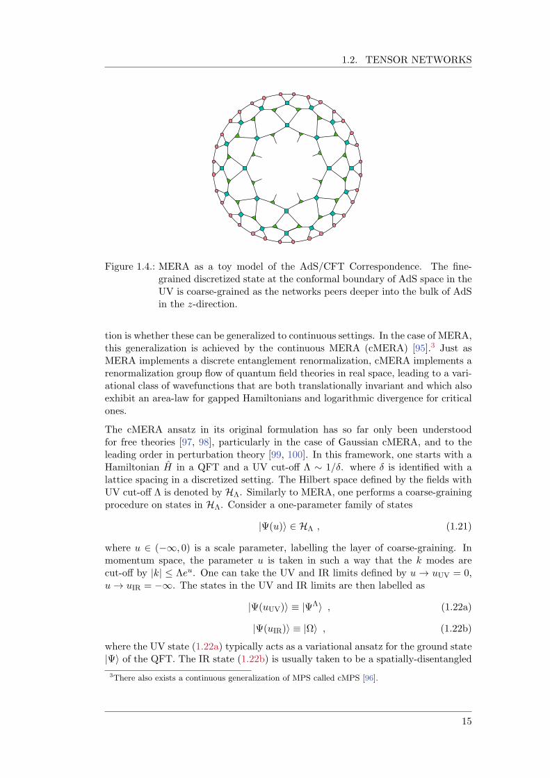
1.2. TENSOR NETWORKS
Figure 1.4.: MERA as a toy model of the AdS/CFT Correspondence. The fine-grained discretized state at the conformal boundary of AdS space in theUV is coarse-grained as the networks peers deeper into the bulk of AdSin the z-direction.
tion is whether these can be generalized to continuous settings. In the case of MERA,this generalization is achieved by the continuous MERA (cMERA) [95].3 Just asMERA implements a discrete entanglement renormalization, cMERA implements arenormalization group flow of quantum field theories in real space, leading to a vari-ational class of wavefunctions that are both translationally invariant and which alsoexhibit an area-law for gapped Hamiltonians and logarithmic divergence for criticalones.
The cMERA ansatz in its original formulation has so far only been understoodfor free theories [97, 98], particularly in the case of Gaussian cMERA, and to theleading order in perturbation theory [99, 100]. In this framework, one starts with aHamiltonian H in a QFT and a UV cut-off Λ 1/. where is identified with alattice spacing in a discretized setting. The Hilbert space defined by the fields withUV cut-off Λ is denoted by HΛ. Similarly to MERA, one performs a coarse-grainingprocedure on states in HΛ. Consider a one-parameter family of states
|Ψ(u)i 2 HΛ , (1.21)
where u 2 (1, 0) is a scale parameter, labelling the layer of coarse-graining. Inmomentum space, the parameter u is taken in such a way that the k modes arecut-off by |k| Λeu. One can take the UV and IR limits defined by u ! uUV = 0,u! uIR = 1. The states in the UV and IR limits are then labelled as
|Ψ(uUV)i |ΨΛi , (1.22a)
|Ψ(uIR)i |Ωi , (1.22b)
where the UV state (1.22a) typically acts as a variational ansatz for the ground state|Ψi of the QFT. The IR state (1.22b) is usually taken to be a spatially-disentangled
3There also exists a continuous generalization of MPS called cMPS [96].
15
CHAPTER 1. INTRODUCTION
product state, such that the entanglement entropy vanishes SA = 0 for any subsys-tem bipartition in the IR state.
The crucial point is that the one-parameter family of states (1.21) can be obtainedfrom the IR state (1.22b) via a quantum circuit defined through a unitary trans-formation
|Ψ(u)i := U(u, uIR) |Ωi P
exp
i
Z u
1du0 (L+ K(u0))
|Ωi , (1.23)
where P denote a path-ordered exponential, the operators L and K(u0) are respect-
ively the generator of scale transformations (coarse-graining) and the entangler. Inother words, L and K are the continuum analogues of the disentanglers u and iso-metries w in the MERA. Note that the unitaries K and u can be thought of asentanglers or disentanglers depending on the direction of the entanglement renor-malization, just as the scalings L and w can be thought of as performing a coarse-or fine-graining. While the scaling operator L is independent of u0 and only dependson the generic properties of the QFT, the entangler K(u0) is theory-dependent andis the basis for the variational ansatz.
The UV state (1.22a) can also be obtained from the on-parameter family (1.21) as|ΨΛi := U(uUV, u) |Ψ(u)i, where |Ψ(u)i is given by (1.23). In this framework, the IRstate |Ωi is invariant under re-scalings L, L |Ωi = 0, since it is a completely spatiallydisentangled state. On the other hand, the operator K(u) generates entanglementfor modes |k| Λeu. One can then see from (1.23) that the UV state |ΨΛi isobtained from the disentangled state |Ωi by a continuous generation of entanglementas the scale parameter varies from 1 to 0. As mentioned before, this process canbe reverted, starting from the UV state and flowing to the IR in which case theoperator K(u) disentangles the system as the operator L coarse-grains it.
The cMERA circuit (1.23) was central to early efforts in defining a notion of com-plexity in quantum field theories [101, 102]. The reason being that it is natural toask what is the minimal number of tensors needed to produce a state. On one hand,if a state is simple, then it should be possible, at least in principle, to produce itusing fewer tensors than a more “complex” state. In this sense, one can heuristicallyassociate a notion of complexity to the number of tensors needed to produce a givenstate. This applies in particular to MERA and cMERA states and is the origin ofcomplexity in quantum-many body systems and quantum fields as studied in thecourse of the past four years.
We review the general notion of complexity arising from quantum circuits for QFTsin Chapter 3. Other proposals to realize an AdS/TN correspondence include thepath-integral optimization approach [103, 104]. More recent efforts to construct TNstates in the AdS/CFT correspondence include [105–107].
1.3. Organization of this thesis
This thesis is organized as follows: Chapter 2 is dedicated to presenting the notionsof entanglement entropy, complexity and related quantities from the perspective of
16
1.3. ORGANIZATION OF THIS THESIS
the AdS/CFT correspondence. The goal of this Chapter is to provide a conceptualbackground for the developments presented in this thesis.
In Chapter 3 we present the mathematical techniques and tools necessary for de-scribing the computation of circuit complexity of vacuum states of free bosonic andfermionic QFTs. We also describe the motivation and geometrical tools developedby Michael Nielsen and collaborators used to study circuit complexity in quantummechanics and which led to the recent implementation of the concept of complexitygeometry in QFTs. The aim of this Chapter is to present the necessary mathem-atical and physical background that will be used in the subsequent chapters of thethesis.
Chapter 4 deals with the study of complexity in a time-dependent setting and isbased on [CamH03]. We do this by considering a smooth quench through a crit-ical point in a free bosonic CFT. We analyse the complexity of the time-dependentground state and study the universal scalings. We show that complexity, like en-tanglement entropy, can be used as a probe of phase transitions in quantum-manybody systems providing a foundation for further studies in this direction.
In Chapter 5 we present the study of complexity of purification, a measure of com-plexity which generalizes the notion from pure to mixed quantum states, basedon [CamH03, CamH02]. We study complexity of purification for vacuum subre-gions of free QFTs and show that complexity of purification captures the divergencestructure of pure state complexity. In the case of two adjacent intervals we showthat complexity of purification exhibits a logarithmic divergence akin to the holo-graphic subregion complexity proposals. We also compare our bosonic complexityof purification results with two other approaches present in the literature.
In Chapter 6, based on [CamH02, CamH01], we present the study of entanglementof purification, a correlation measure which generalizes the notion of entanglemententropy to mixed states, and of reflected entropy, another correlation measure builtfrom the so-called canonical purification We first focus on entanglement of purifica-tion, and discuss its behaviour for vacuum subregions of free CFT consisting of twoadjacent intervals. We show that it behaves in agreement both with holographicand CFT expectations. We then compare our results for entanglement of purific-ation and reflected entropy for subregions of free CFTs consisting of two disjointintervals which are largely separated from each other. Here we focus specifically onthe c = 1/2 Ising CFT and show that both entanglement of purification and reflectedentropy present a logarithmic enhancement with respect to the leading power-lawdivergence in the separation, a feature which provides new insights into the largedistance behaviour of these correlation measures.
Finally, in Chapter 7 we discuss the developments presented in this thesis, theirsignificance in the current state of research in this field and future directions.
17

CHAPTER 1. INTRODUCTION
18
2. Quantum Information Aspects of the AdS/CFT
Correspondence
In this Chapter we review recent developments in the AdS/CFT correspondencethat have been motivated by connections between quantum gravity and quantuminformation. We start with a discussion of holographic entanglement entropy andthe Ryu–Takayanagi formula in Sec. 2.1.1. We follow this discussion by a review ofentanglement wedge reconstruction and the holographic interpretation of its crosssection in Sec. 2.2. Finally, we present the holographic complexity proposals inSec. 2.3 as well as the holographic subregion complexity proposals. By the end ofthis Chapter, we will have motivated the study of quantum information-theoreticquantities such as complexity, entanglement of purification and reflected entropy inthe context of quantum field theories.
2.1. Holographic Entanglement Entropy
Entanglement is a fundamental property of quantum systems that distinguishes themfrom classical ones. A particular notion of it, entanglement entropy (EE) (1.18),has played a key role in recent developments in quantum field theory (QFT) and ingravity through the AdS/CFT correspondence for more than two decades. This hasbeen motivated on one hand by the study of black hole entropy (1.1) and quantumgravity, and on the other by the study of quantum many-body systems in condensedmatter physics.
In the former case, it was understood that the leading UV divergent term in theentropy of a region is proportional to its surface area [108–111] and therefore blackhole entropy SBH must be understood, at least to some extent, as arising fromthe entanglement of quantum fields across its horizon H . This in turn inspireda deeper study of EE in QFTs, where useful techniques such as the replica trickwere developed [85, 112] and which led to a variety of results in (1 + 1)-dimensionalconformal field theories (CFTs) [86, 113], in gapped systems [114], topological set-ups [115, 116], and related to the quantum Hall effect [117].
In the context of high-energy physics and particularly within the AdS/CFT com-munity, the proposal of Shinsei Ryu and Tadashi Takayanagi [118, 119] representsarguably the most groundbreaking discovery since Maldacena’s conjecture. It isalso one of the first and most representative connections between AdS/CFT andquantum-information, together with Swingle’s description of MERA as a toy modelof AdS (see Fig. 1.4).
19
CHAPTER 2. QUANTUM INFORMATION ASPECTS OF THE ADS/CFTCORRESPONDENCE
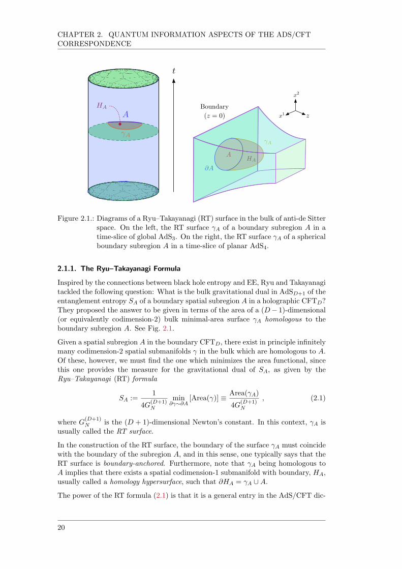
Figure 2.1.: Diagrams of a Ryu–Takayanagi (RT) surface in the bulk of anti-de Sitterspace. On the left, the RT surface A of a boundary subregion A in atime-slice of global AdS3. On the right, the RT surface A of a sphericalboundary subregion A in a time-slice of planar AdS4.
2.1.1. The Ryu–Takayanagi Formula
Inspired by the connections between black hole entropy and EE, Ryu and Takayanagitackled the following question: What is the bulk gravitational dual in AdSD+1 of theentanglement entropy SA of a boundary spatial subregion A in a holographic CFTD?They proposed the answer to be given in terms of the area of a (D 1)-dimensional(or equivalently codimension-2) bulk minimal-area surface A homologous to theboundary subregion A. See Fig. 2.1.
Given a spatial subregion A in the boundary CFTD, there exist in principle infinitelymany codimension-2 spatial submanifolds in the bulk which are homologous to A.Of these, however, we must find the one which minimizes the area functional, sincethis one provides the measure for the gravitational dual of SA, as given by theRyu–Takayanagi (RT) formula
SA :=1
4G(D+1)N
min∂γ∂A
[Area()] Area(A)
4G(D+1)N
, (2.1)
where G(D+1)N is the (D + 1)-dimensional Newton’s constant. In this context, A is
usually called the RT surface.
In the construction of the RT surface, the boundary of the surface A must coincidewith the boundary of the subregion A, and in this sense, one typically says that theRT surface is boundary-anchored. Furthermore, note that A being homologous toA implies that there exists a spatial codimension-1 submanifold with boundary, HA,usually called a homology hypersurface, such that @HA = A [A.
The power of the RT formula (2.1) is that it is a general entry in the AdS/CFT dic-
20
2.1. HOLOGRAPHIC ENTANGLEMENT ENTROPY
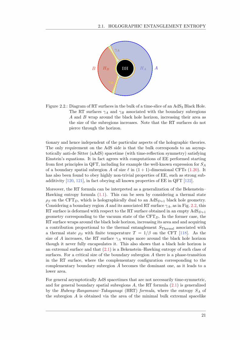
Figure 2.2.: Diagram of RT surfaces in the bulk of a time-slice of an AdS3 Black Hole.The RT surfaces A and B associated with the boundary subregionsA and B wrap around the black hole horizon, increasing their area asthe size of the subregions increases. Note that the RT surfaces do notpierce through the horizon.
tionary and hence independent of the particular aspects of the holographic theories.The only requirement on the AdS side is that the bulk corresponds to an asymp-totically anti-de Sitter (aAdS) spacetime (with time-reflection symmetry) satisfyingEinstein’s equations. It in fact agrees with computations of EE performed startingfrom first principles in QFT, including for example the well-known expression for SA
of a boundary spatial subregion A of size ` in (1 + 1)-dimensional CFTs (1.20). Ithas also been found to obey highly non-trivial properties of EE, such as strong sub-additivity [120, 121], in fact obeying all known properties of EE in QFT [122].
Moreover, the RT formula can be interpreted as a generalization of the Bekenstein–Hawking entropy formula (1.1). This can be seen by considering a thermal stateβ on the CFTD, which is holographically dual to an AdSD+1 black hole geometry.Considering a boundary region A and its associated RT surface A, as in Fig. 2.2, thisRT surface is deformed with respect to the RT surface obtained in an empty AdSD+1
geometry corresponding to the vacuum state of the CFTD. In the former case, theRT surface wraps around the black hole horizon, increasing its area and and acquiringa contribution proportional to the thermal entanglement SThermal associated witha thermal state β with finite temperature T = 1/ on the CFT [118]. As thesize of A increases, the RT surface A wraps more around the black hole horizonthough it never fully encapsulates it. This also shows that a black hole horizon isan extremal surface and that (2.1) is a Bekenstein–Hawking entropy of such class ofsurfaces. For a critical size of the boundary subregion A there is a phase-transitionin the RT surface, where the complementary configuration corresponding to thecomplementary boundary subregion A becomes the dominant one, as it leads to alower area.
For general asymptotically AdS spacetimes that are not necessarily time-symmetric,and for general boundary spatial subregions A, the RT formula (2.1) is generalizedby the Hubeny–Rangamani–Takayanagi (HRT) formula, where the entropy SA ofthe subregion A is obtained via the area of the minimal bulk extremal spacelike
21
CHAPTER 2. QUANTUM INFORMATION ASPECTS OF THE ADS/CFTCORRESPONDENCE
hypersurface homologous to A [123]. In this context, the area of A is taken to beextremal under small variations of its position in spacetime [124], provided @A =@A. In this case, A is said to be minimal in the sense that there is no otherhypersurface with a strictly smaller area which satisfies these conditions.
The RT formula was proven within the AdS/CFT correspondence for (1 + 1)-dimensional CFTs in [125, 126] and subsequently for more general scenarios in [127].In particular, the HRT formula was proven in [128] by implementing the Schwinger-Keldysh construction [129–131] on the bulk side in order to compute the reduceddensity matrix of a boundary subregion. In the context of spherical vacuum subre-gions for arbitrary dimensions, the RT formula was proven in [132]. However, theRT formula and its covariant generalization, the HRT formula, hold only for classicalbulk spacetimes satisfying Einstein’s equations.
Beyond Einstein gravity, there are generalizations of these formulas for classicalbulk geometries arising from higher-derivative gravitational theories [133] such asLovelock theories [134, 135]. There also exist conjectured generalizations for 3-dimensional Chern–Simons theories [136] and higher-spin gravity [137].
Beyond classical gravitational theories, there must to be quantum corrections tothe RT formula appearing as a perturbative expansion in GN . At order G0
N suchcorrection is given by a semiclassical treatment of the bulk fields,i.e., by treatingthem as quantum fields on a fixed classical background and computing SA for thehomology hypersurface HA. The expression containing this quantum correction isknown as the Faulkner–Lewkowycz–Maldacena (FLM) formula [138], for which thereexists a conjectured generalization to all-orders in O(1/GN ) [139]. Precious little isknown beyond such perturbative quantum corrections to RT, but they are thoughtto be relevant for smoothening phase transitions of RT surfaces e.g., in the presenceof a black hole.
In this regard, it was further argued in [139] that in the presence of quantum fields,the RT prescription needs to be modified in order to account for the entropy arisingfrom the entanglement of the quantum fields across the minimal (or extremal) sur-face A. This observation is the natural holographic analogue of the generalizedsecond law of black hole thermodynamics [43]. In this construction, one has thatthe holographic entanglement entropy of a boundary subregion A is given by
SA := min ext(Sgen()) = min∂γ∂A
(ext
Area()
4G(D+1)N
+ Sbulk()
!), (2.2)
where is the bulk surface homologous to the boundary subregion A, and whereSbulk() is the entropy of quantum fields in the homology hypersurface HA. Thesurface which extremizes the generalized entropy is called a quantum extremalsurface (QES) [139]. In formula (2.2) one first needs to find the surface whichextremizes the generalized entropy Sgen() and in case there is more than one surfacewhich does this, then one needs to choose the one yielding the minimum value ofSgen().
This approach has led to novel insights in holographic models of black hole evapor-ation and in particular it has been used to compute the Page curve in a controlled
22
2.2. THE ENTANGLEMENT WEDGE
manner [18, 19, 140]. The surprising aspect, as we mentioned in the Introduction 1,is that the Page curve can be obtained from semi-classical gravity computationsinvolving saddle points for the QES. In this case, the computation of the EE of theHawking radiation is encapsulated by the island formula [140]. While we will notexplore the details of this construction and the consequences of the island formula,we would be remiss not to mention its relevance in understanding this crucial aspectof unitary black hole evaporation. Despite this significant breakthrough, however,we cannot claim that the black hole information paradox has been resolved. In fact,as we will discuss in the later sections of this chapter, it can be argued that onerequires additional information about the quantum state involved int he black holeevaporation process beyond what can be captured by entanglement entropy.
2.2. The Entanglement Wedge
Perhaps the most fascinating aspect of the AdS/CFT correspondence is that itrelates a quantum theory of gravity to a theory without it. In the regime wherethe quantum theory is strongly-coupled this duality relates such a theory with aclassical theory of gravity. This, as we have mentioned, has led to new insightsinto the properties of strongly-coupled theories. However from a fundamental per-spective, the correspondence has also opened the path to understand gravity froma different perspective; that of a quantum theory without gravitational degrees offreedom.
Indeed, an idea which has taken a central role in recent investigations of the Ad-S/CFT correspondence is that gravity, at least when it pertains to the physics onnegatively-curved spaces, is an emergent phenomenon. This idea was argued by MarkVan Raamsdonk, stating that an essential ingredient in the emergence of spacetimeis quantum entanglement [141]. Van Raamsdonk’s claim was that the connectiv-ity between different regions in spacetime could be seen as a consequence of theentanglement between them. This proposal was motivated by Maldacena’s observa-tion that the eternal AdS black hole geometry is obtained by maximally-entanglingtwo spatially-separated copies of a CFT in a thermal state which are initially un-entangled form each other [142], see Fig. 2.3. In said entangled state of two copiesof the CFT, entanglement is measured by the mutual information (MI)
I(A : B) := SA + SB SA[B , (2.3)
where here A and B represent spatial subregions on the entangled CFT states. In thecontext of the AdS/CFT correspondence, the behaviour of MI has been understoodas a function of the distance between subsystems A and B [143, 144]. Furthermore,it is also an upper-bound to two-point correlation functions [145], which are expectedto decay exponentially with the bulk geodesic distance [144]. This means that anincrement in the entanglement implies a shorter bulk distance between the subsys-tems and viceversa. This observation was then taken as heuristically implying thatentanglement between the subregions is responsible for binding the bulk spacetimebetween them.
Though the precise connection between entanglement and the emergence of grav-ity has not been rigorously established or even understood, it has led to new in-
23
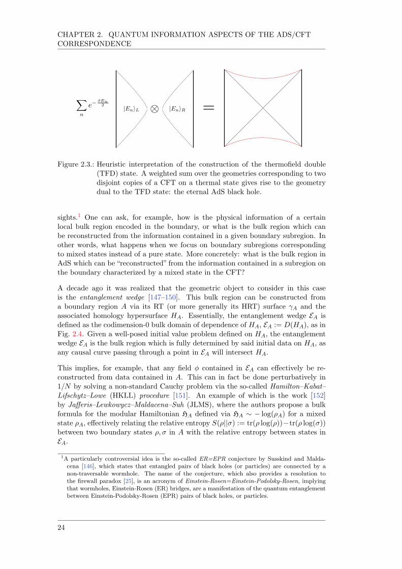
CHAPTER 2. QUANTUM INFORMATION ASPECTS OF THE ADS/CFTCORRESPONDENCE
Figure 2.3.: Heuristic interpretation of the construction of the thermofield double(TFD) state. A weighted sum over the geometries corresponding to twodisjoint copies of a CFT on a thermal state gives rise to the geometrydual to the TFD state: the eternal AdS black hole.
sights.1 One can ask, for example, how is the physical information of a certainlocal bulk region encoded in the boundary, or what is the bulk region which canbe reconstructed from the information contained in a given boundary subregion. Inother words, what happens when we focus on boundary subregions correspondingto mixed states instead of a pure state. More concretely: what is the bulk region inAdS which can be “reconstructed” from the information contained in a subregion onthe boundary characterized by a mixed state in the CFT?
A decade ago it was realized that the geometric object to consider in this caseis the entanglement wedge [147–150]. This bulk region can be constructed froma boundary region A via its RT (or more generally its HRT) surface A and theassociated homology hypersurface HA. Essentially, the entanglement wedge EA isdefined as the codimension-0 bulk domain of dependence of HA, EA := D(HA), as inFig. 2.4. Given a well-posed initial value problem defined on HA, the entanglementwedge EA is the bulk region which is fully determined by said initial data on HA, asany causal curve passing through a point in EA will intersect HA.
This implies, for example, that any field contained in EA can effectively be re-constructed from data contained in A. This can in fact be done perturbatively in1/N by solving a non-standard Cauchy problem via the so-called Hamilton–Kabat–Lifschytz–Lowe (HKLL) procedure [151]. An example of which is the work [152]by Jafferis–Lewkowycz–Maldacena–Suh (JLMS), where the authors propose a bulkformula for the modular Hamiltonian HA defined via HA log(A) for a mixedstate A, effectively relating the relative entropy S(||) := tr( log())tr( log())between two boundary states , in A with the relative entropy between states inEA.
1A particularly controversial idea is the so-called ER=EPR conjecture by Susskind and Malda-cena [146], which states that entangled pairs of black holes (or particles) are connected by anon-traversable wormhole. The name of the conjecture, which also provides a resolution tothe firewall paradox [25], is an acronym of Einstein-Rosen=Einstein-Podolsky-Rosen, implyingthat wormholes, Einstein-Rosen (ER) bridges, are a manifestation of the quantum entanglementbetween Einstein-Podolsky-Rosen (EPR) pairs of black holes, or particles.
24
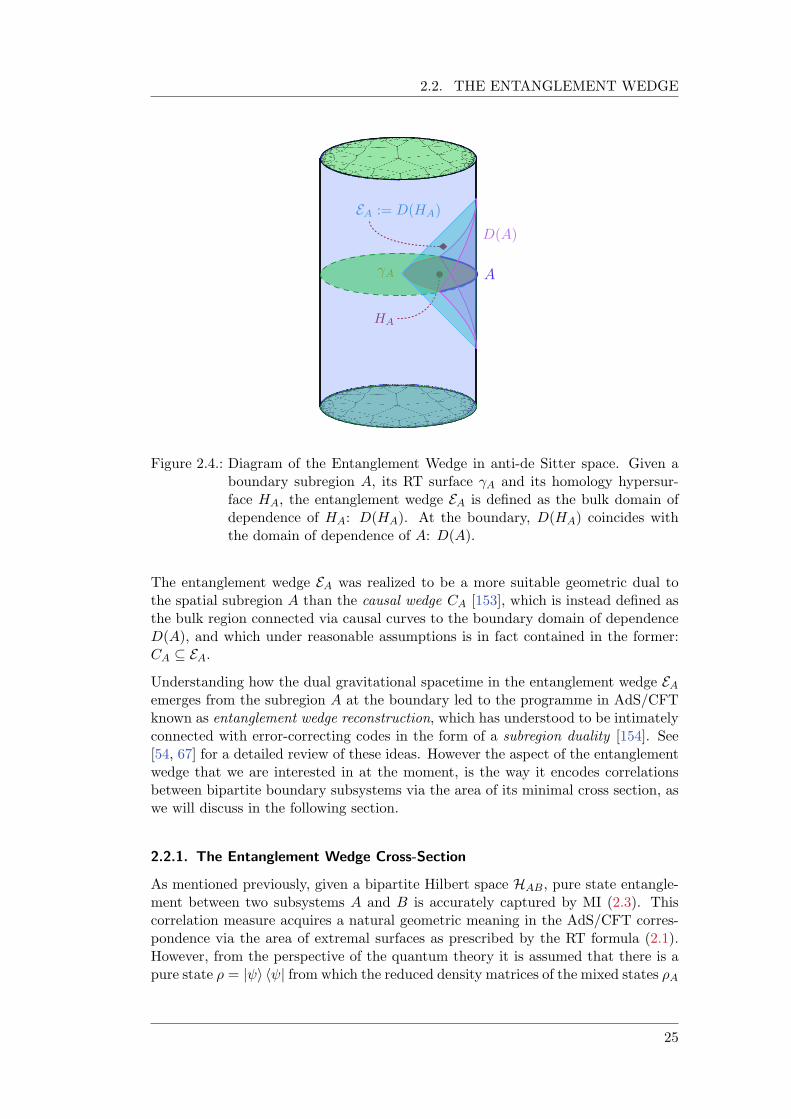
2.2. THE ENTANGLEMENT WEDGE
Figure 2.4.: Diagram of the Entanglement Wedge in anti-de Sitter space. Given aboundary subregion A, its RT surface A and its homology hypersur-face HA, the entanglement wedge EA is defined as the bulk domain ofdependence of HA: D(HA). At the boundary, D(HA) coincides withthe domain of dependence of A: D(A).
The entanglement wedge EA was realized to be a more suitable geometric dual tothe spatial subregion A than the causal wedge CA [153], which is instead defined asthe bulk region connected via causal curves to the boundary domain of dependenceD(A), and which under reasonable assumptions is in fact contained in the former:CA EA.
Understanding how the dual gravitational spacetime in the entanglement wedge EAemerges from the subregion A at the boundary led to the programme in AdS/CFTknown as entanglement wedge reconstruction, which has understood to be intimatelyconnected with error-correcting codes in the form of a subregion duality [154]. See[54, 67] for a detailed review of these ideas. However the aspect of the entanglementwedge that we are interested in at the moment, is the way it encodes correlationsbetween bipartite boundary subsystems via the area of its minimal cross section, aswe will discuss in the following section.
2.2.1. The Entanglement Wedge Cross-Section
As mentioned previously, given a bipartite Hilbert space HAB, pure state entangle-ment between two subsystems A and B is accurately captured by MI (2.3). Thiscorrelation measure acquires a natural geometric meaning in the AdS/CFT corres-pondence via the area of extremal surfaces as prescribed by the RT formula (2.1).However, from the perspective of the quantum theory it is assumed that there is apure state = | i h | from which the reduced density matrices of the mixed states A
25
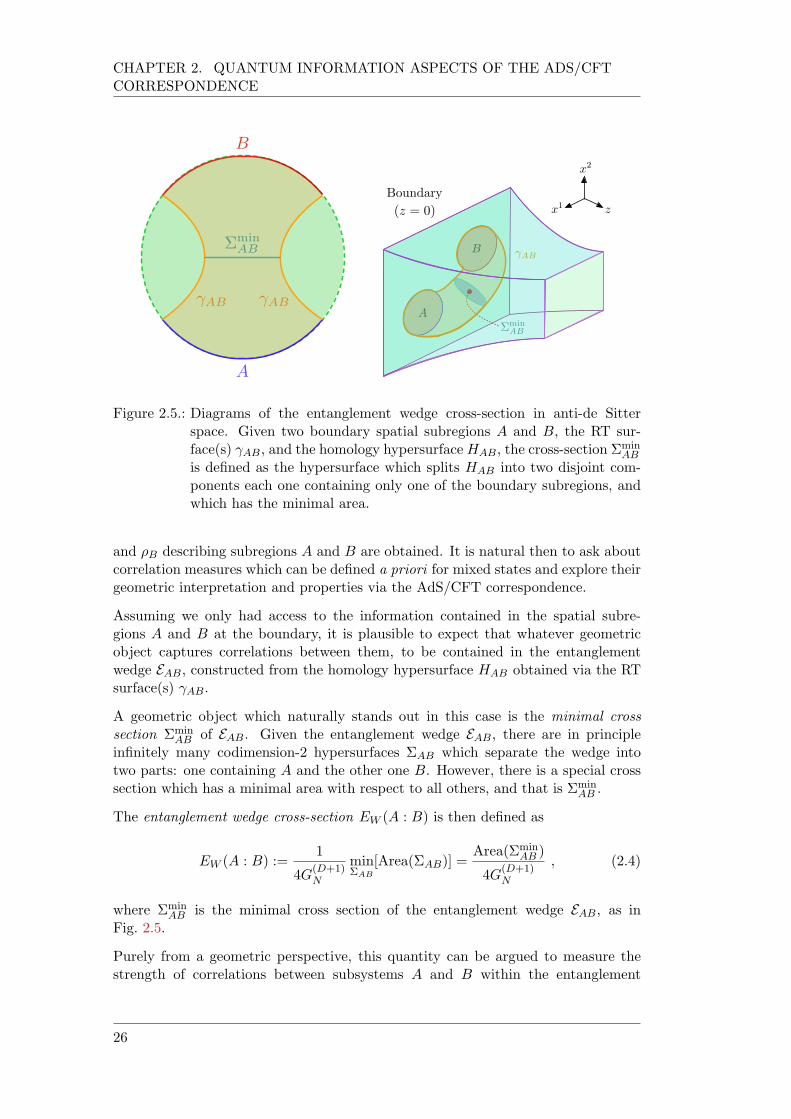
CHAPTER 2. QUANTUM INFORMATION ASPECTS OF THE ADS/CFTCORRESPONDENCE
Figure 2.5.: Diagrams of the entanglement wedge cross-section in anti-de Sitterspace. Given two boundary spatial subregions A and B, the RT sur-face(s) AB, and the homology hypersurfaceHAB, the cross-section Σ
minAB
is defined as the hypersurface which splits HAB into two disjoint com-ponents each one containing only one of the boundary subregions, andwhich has the minimal area.
and B describing subregions A and B are obtained. It is natural then to ask aboutcorrelation measures which can be defined a priori for mixed states and explore theirgeometric interpretation and properties via the AdS/CFT correspondence.
Assuming we only had access to the information contained in the spatial subre-gions A and B at the boundary, it is plausible to expect that whatever geometricobject captures correlations between them, to be contained in the entanglementwedge EAB, constructed from the homology hypersurface HAB obtained via the RTsurface(s) AB.
A geometric object which naturally stands out in this case is the minimal crosssection Σ
minAB of EAB. Given the entanglement wedge EAB, there are in principle
infinitely many codimension-2 hypersurfaces ΣAB which separate the wedge intotwo parts: one containing A and the other one B. However, there is a special crosssection which has a minimal area with respect to all others, and that is Σmin
AB .
The entanglement wedge cross-section EW (A : B) is then defined as
EW (A : B) :=1
4G(D+1)N
minΣAB
[Area(ΣAB)] =Area(Σmin
AB )
4G(D+1)N
, (2.4)
where ΣminAB is the minimal cross section of the entanglement wedge EAB, as in
Fig. 2.5.
Purely from a geometric perspective, this quantity can be argued to measure thestrength of correlations between subsystems A and B within the entanglement
26
2.2. THE ENTANGLEMENT WEDGE
wedge, since it reduces to EE if the total system AB is in a pure state EW (A :B) = SA = SB and because it also satisfies the following bounds [155]
1
2I(A : B) EW (A : B) min[SA, SB] , (2.5)
as well as strong subadditivity
EW (AB CD) EW (AB) + EW (CD) . (2.6)
However in [156, 157] authors went beyond this general connection and conjecturedthe entanglement wedge cross-section EW to be dual to a mixed state generalizationof EE known as the entanglement of purification (EoP)
EW (A : B) EP (A : B) , (2.7)
where this expression holds to the leading order in N and for all CFTs with aholographic dual. EoP is a measure of total correlations between two subsystemsthat includes both classical and quantum correlations [158, 159], and which is wellknown in the quantum information community.
Given a mixed state in a bipartite Hilbert space HAB with reduced density mat-rix AB : HAB ! HAB, one can construct a purification | i 2 H of AB byextending the Hilbert space HAB according to HAB ! HAB HA0B0 , such thatAB = trA0B0(| i h |). The EoP, EP (AB) EP (A : B), is then defined as theminimum of the entanglement entropy S(A [ A0) = SAA0 = trAA0(AA0 log(AA0))for the reduced density matrix AA0 = trBB0(| i h |) with respect to all possiblepurifications | i 2 H.
The conjecture (2.7) was based on tensor network interpretations of the AdS/CFTcorrespondence, supported by CFT techniques in specific examples [160] and hassince been an active topic of research [161–168], which strongly motivates its studyin QFTs, being one of the main objectives of this thesis.
The main obstacle, or perhaps the unsatisfactory aspect of EoP, is that it intrins-ically requires to solve a challenging minimization procedure, in principle over allpossible purifications of the given mixed state. This makes any efforts to test theconjecture (2.7) equally challenging.
Because of this, authors in [169] proposed a “simpler” holographic dual to the entan-glement wedge cross section EW which does not require any minimization like EoP.They argued that in QFTs with a holographic dual, a quantity known as reflectedentropy SR is also dual to EW . They proposed the identification
EW (A : B) 1
2SR(A : B) , (2.8)
which they conjectured to be valid to leading order in N and also for all CFTs witha holographic dual.
For a bipartite quantum system HAB, the reflected entropy (RE) SR of a mixedstate AB is defined as the von-Neumann entropy
SR(AB) := S (trBB0 (|pABi h
pAB|)) , (2.9)
27
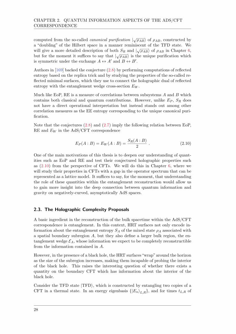
CHAPTER 2. QUANTUM INFORMATION ASPECTS OF THE ADS/CFTCORRESPONDENCE
computed from the so-called canonical purification |pABi of AB, constructed by
a “doubling” of the Hilbert space in a manner reminiscent of the TFD state. Wewill give a more detailed description of both SR and |
pABi of AB in Chapter 6,
but for the moment it suffices to say that |pABi is the unique purification which
is symmetric under the exchange A$ A0 and B $ B0.
Authors in [169] backed the conjecture (2.8) by performing computations of reflectedentropy based on the replica trick and by studying the properties of the so-called re-flected minimal surfaces, which they use to connect the holographic dual of reflectedentropy with the entanglement wedge cross-section EW .
Much like EoP, RE is a measure of correlations between subsystems A and B whichcontains both classical and quantum contributions. However, unlike EP , SR doesnot have a direct operational interpretation but instead stands out among othercorrelation measures as the EE entropy corresponding to the unique canonical puri-fication.
Note that the conjectures (2.8) and (2.7) imply the following relation between EoP,RE and EW in the AdS/CFT correspondence
EP (A : B) = EW (A : B) =SR(A : B)
2. (2.10)
One of the main motivations of this thesis is to deepen our understanding of quant-ities such as EoP and RE and test their conjectured holographic properties suchas (2.10) from the perspective of CFTs. We will do this in Chapter 6, where wewill study their propreties in CFTs with a gap in the operator spectrum that can berepresented as a lattice model. It suffices to say, for the moment, that understandingthe role of these quantities within the entanglement reconstruction would allow usto gain more insight into the deep connection between quantum information andgravity on negatively-curved, asymptotically AdS spaces.
2.3. The Holographic Complexity Proposals
A basic ingredient in the reconstruction of the bulk spacetime within the AdS/CFTcorrespondence is entanglement. In this context, HRT surfaces not only encode in-formation about the entanglement entropy SA of the mixed state A associated witha spatial boundary subregion A, but they also define a larger bulk region, the en-tanglement wedge EA, whose information we expect to be completely reconstructiblefrom the information contained in A.
However, in the presence of a black hole, the HRT surfaces“wrap”around the horizonas the size of the subregion increases, making them incapable of probing the interiorof the black hole. This raises the interesting question of whether there exists aquantity on the boundary CFT which has information about the interior of theblack hole.
Consider the TFD state |TFDi, which is constructed by entangling two copies of aCFT in a thermal state. In an energy eigenbasis |EniL,R, and for times tL,R of
28
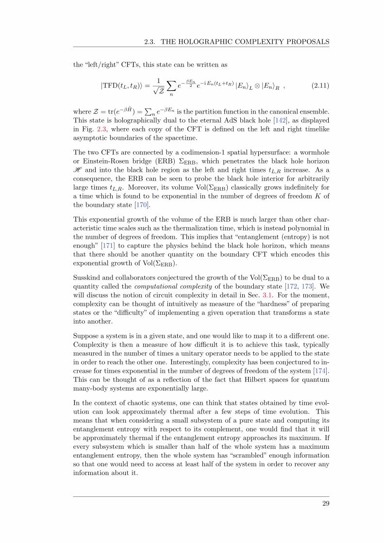
2.3. THE HOLOGRAPHIC COMPLEXITY PROPOSALS
the “left/right” CFTs, this state can be written as
|TFD(tL, tR)i =1pZ
X
n
eβEn2 eiEn(tL+tR) |EniL |EniR , (2.11)
where Z = tr(eβH) =P
n eβEn is the partition function in the canonical ensemble.
This state is holographically dual to the eternal AdS black hole [142], as displayedin Fig. 2.3, where each copy of the CFT is defined on the left and right timelikeasymptotic boundaries of the spacetime.
The two CFTs are connected by a codimension-1 spatial hypersurface: a wormholeor Einstein-Rosen bridge (ERB) ΣERB, which penetrates the black hole horizonH and into the black hole region as the left and right times tL,R increase. As aconsequence, the ERB can be seen to probe the black hole interior for arbitrarilylarge times tL,R. Moreover, its volume Vol(ΣERB) classically grows indefinitely fora time which is found to be exponential in the number of degrees of freedom K ofthe boundary state [170].
This exponential growth of the volume of the ERB is much larger than other char-acteristic time scales such as the thermalization time, which is instead polynomial inthe number of degrees of freedom. This implies that “entanglement (entropy) is notenough” [171] to capture the physics behind the black hole horizon, which meansthat there should be another quantity on the boundary CFT which encodes thisexponential growth of Vol(ΣERB).
Susskind and collaborators conjectured the growth of the Vol(ΣERB) to be dual to aquantity called the computational complexity of the boundary state [172, 173]. Wewill discuss the notion of circuit complexity in detail in Sec. 3.1. For the moment,complexity can be thought of intuitively as measure of the “hardness” of preparingstates or the “difficulty” of implementing a given operation that transforms a stateinto another.
Suppose a system is in a given state, and one would like to map it to a different one.Complexity is then a measure of how difficult it is to achieve this task, typicallymeasured in the number of times a unitary operator needs to be applied to the statein order to reach the other one. Interestingly, complexity has been conjectured to in-crease for times exponential in the number of degrees of freedom of the system [174].This can be thought of as a reflection of the fact that Hilbert spaces for quantummany-body systems are exponentially large.
In the context of chaotic systems, one can think that states obtained by time evol-ution can look approximately thermal after a few steps of time evolution. Thismeans that when considering a small subsystem of a pure state and computing itsentanglement entropy with respect to its complement, one would find that it willbe approximately thermal if the entanglement entropy approaches its maximum. Ifevery subsystem which is smaller than half of the whole system has a maximumentanglement entropy, then the whole system has “scrambled” enough informationso that one would need to access at least half of the system in order to recover anyinformation about it.
29
CHAPTER 2. QUANTUM INFORMATION ASPECTS OF THE ADS/CFTCORRESPONDENCE
Figure 2.6.: Pictorial representation of the time evolution of complexity in strongly-coupled system, conjectured in [174] and recently proven in [176] forrandom quantum circuits. Quantum circuit complexity exhibits a lineargrowth for times of the order O(eK) where K is the number of degreesof freedom of the quantum state. Quantum recurrences are expected tooccur at double exponential times ee
Kbringing the complexity down to
its initial value.
One typically expects that the so-called scrambling time in a system described byan interacting Hamiltonian scales as the logarithm of the degrees of freedom of thesystem, while complexity still increases for exponentially large times. In this sense,one typically expects the complexity of a state in a chaotic system to increase forlong times, even after the thermalization of perturbations. For longer times, doublyexponential in the number of degrees of freedom, one typically expects quantumrecurrences to occur so that the system returns to its initial state [175].
In the regime of linear growth, complexity C is conjectured to increase proportionallyto the energy E of the system
dC
dt
teK
E , (2.12)
where K is the number of degrees of freedom of the system, see Fig. 2.6. It isimportant to mention that this linear growth of complexity conjectured in [174] hasrecently been proven in [176] for random quantum circuits.
Returnig to the discussion regarding the volume of the ERB; the fact that thereis a property of the bulk geometry that keeps increasing for much longer timeseven though the entanglement has thermalized is what motivated Susskind andcollaborators to argue that the growth of the volume of the ERB captures propertiesof the complexity of the time evolution of the TFD state.
2.3.1. Actions and Volumes
Motivated by the analogy between the growth of the black hole interior as measuredby the volume of the ERB and the growth of computational complexity, Susskind
30
2.3. THE HOLOGRAPHIC COMPLEXITY PROPOSALS
proposed the notion of holographic complexity as the quantity which encodes thisevolution of the ERB from the perspective of the boundary CFT.
Together with collaborators, he proposed two gravitational observables which accur-ately capture the late time growth of the ERB. The first one of these is known as the“complexity=volume” (CV) proposal [170, 173], which postulates that the complex-ity of the boundary state is proportional to the volume of a maximal codimension-1bulk hypersurface B that extends to the asymptotic boundary and which asymptotesto the time slice Σ where the boundary state is defined
CV[Σ] :=1
`bulkG(D+1)N
maxΣ=∂B
[Vol(B)] =Vol(Σmax)
`bulkG(D+1)N
, (2.13)
where `bulk is an arbitrary length scale needed to make complexity dimensionlessand which is typically chosen to be the AdS radius L, though certain authors [177]proposed a sophisticated approach in order to determine this length scale. In thecase of the eternal AdS black hole, this bulk surface connects the time slices at timestL,R through the ERB, as shown on the left side in Fig. 2.7.
The second conjecture goes by the name of “complexity=action” (CA) proposal [178,179] and identifies the complexity of the boundary state with the gravitational actionIG evaluated on a codimension-0 bulk region known as theWheeler-De Witt (WDW)patch
CA[Σ] :=IG[WWDW]
=
IWDW
, (2.14)
where the WDW patch WWDW is defined as the causal development of the spacelikehypersurface Σ
max singled out by the CV construction, as shown on the right sidein Fig. 2.7. The factor of 1/ was a chosen by authors of [178, 179] in an attemptto connect to a suggestion that computation rates are bounded, a conjecture knownas Lloyd’s bound [180]. However, that this bound is generically violated in the CAproposal [181].
This gravitational action IG consists of various terms which include the bulk actionIBulk, proportional to the spacetime volume of the WDW patch Vol(WWDW), as wellas a Gibbons–Hawking–York term defined on the timelike and spacelike boundaries,as well as other terms arising from the null boundaries [182, 183], Hayward (joint)terms [184, 185] and counter-terms. A third conjecture, the “complexity=volume2.0” (CV2) proposal [186] was proposed some years later stating that the complexityof the boundary state is instead identified with the spacetime volume of the WDWpatch
CV2.0 [Σ] :=fVol(WWDW)
L2G(D+1)N
. (2.15)
The properties of these holographic complexity conjectures have been studied in avariety of settings and the structure of their UV divergences has been understoodin several asymptotically AdS spacetimes [181, 187–192].
31
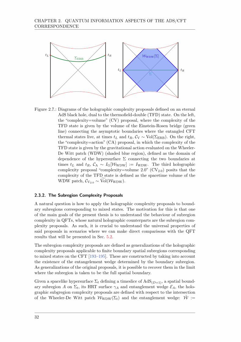
CHAPTER 2. QUANTUM INFORMATION ASPECTS OF THE ADS/CFTCORRESPONDENCE
Figure 2.7.: Diagrams of the holographic complexity proposals defined on an eternalAdS black hole, dual to the thermofield-double (TFD) state. On the left,the “complexity=volume” (CV) proposal, where the complexity of theTFD state is given by the volume of the Einstein-Rosen bridge (greenline) connecting the asymptotic boundaries where the entangled CFTthermal states live, at times tL and tR, CV Vol(ΣERB). On the right,the “complexity=action” (CA) proposal, in which the complexity of theTFD state is given by the gravitational action evaluated on the Wheeler-De Witt patch (WDW) (shaded blue region), defined as the domain ofdependence of the hypersurface Σ connecting the two boundaries attimes tL and tR, CA IG[WWDW] := IWDW. The third holographiccomplexity proposal “complexity=volume 2.0” (CV2.0) posits that thecomplexity of the TFD state is defined as the spacetime volume of theWDW patch, CV2.0 fVol(WWDW).
2.3.2. The Subregion Complexity Proposals
A natural question is how to apply the holographic complexity proposals to bound-ary subregions corresponding to mixed states. The motivation for this is that oneof the main goals of the present thesis is to understand the behaviour of subregioncomplexity in QFTs, whose natural holographic counterparts are the subregion com-plexity proposals. As such, it is crucial to understand the universal properties ofsaid proposals in scenarios where we can make direct comparisons with the QFTresults that will be presented in Sec. 5.2.
The subregion complexity proposals are defined as generalizations of the holographiccomplexity proposals applicable to finite boundary spatial subregions correspondingto mixed states on the CFT [193–195]. These are constructed by taking into accountthe existence of the entangelement wedge determined by the boundary subregion.As generalizations of the original proposals, it is possible to recover them in the limitwhere the subregion is taken to be the full spatial boundary.
Given a spacelike hypersurface Σt defining a timeslice of AdS(D+1), a spatial bound-ary subregion A on Σt, its HRT surface A and entanglement wedge EA, the holo-graphic subgregion complexity proposals are defined with respect to the intersectionof the Wheeler-De Witt patch WWDW(Σt) and the entanglement wedge: W :=
32
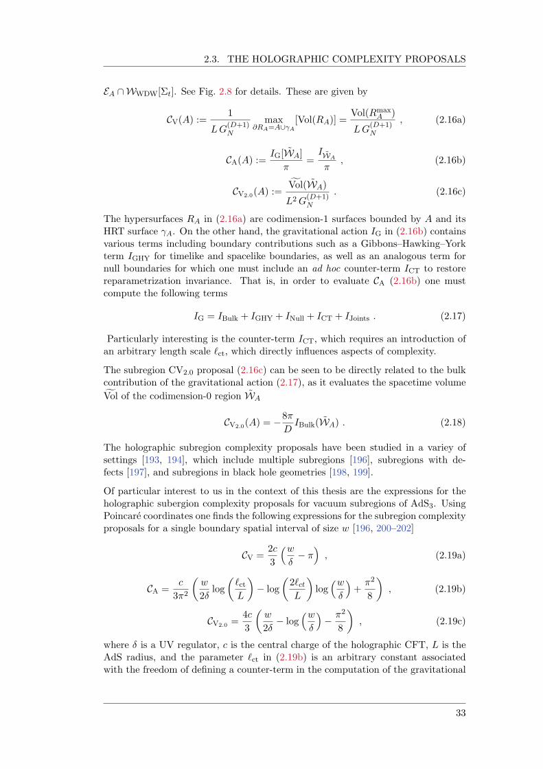
2.3. THE HOLOGRAPHIC COMPLEXITY PROPOSALS
EA \WWDW[Σt]. See Fig. 2.8 for details. These are given by
CV(A) :=1
LG(D+1)N
max∂RA=A[γA
[Vol(RA)] =Vol(Rmax
A )
LG(D+1)N
, (2.16a)
CA(A) :=IG[WA]
=
IWA
, (2.16b)
CV2.0(A) :=fVol(WA)
L2G(D+1)N
. (2.16c)
The hypersurfaces RA in (2.16a) are codimension-1 surfaces bounded by A and itsHRT surface A. On the other hand, the gravitational action IG in (2.16b) containsvarious terms including boundary contributions such as a Gibbons–Hawking–Yorkterm IGHY for timelike and spacelike boundaries, as well as an analogous term fornull boundaries for which one must include an ad hoc counter-term ICT to restorereparametrization invariance. That is, in order to evaluate CA (2.16b) one mustcompute the following terms
IG = IBulk + IGHY + INull + ICT + IJoints . (2.17)
Particularly interesting is the counter-term ICT, which requires an introduction ofan arbitrary length scale `ct, which directly influences aspects of complexity.
The subregion CV2.0 proposal (2.16c) can be seen to be directly related to the bulkcontribution of the gravitational action (2.17), as it evaluates the spacetime volumefVol of the codimension-0 region WA
CV2.0(A) = 8
DIBulk(WA) . (2.18)
The holographic subregion complexity proposals have been studied in a variey ofsettings [193, 194], which include multiple subregions [196], subregions with de-fects [197], and subregions in black hole geometries [198, 199].
Of particular interest to us in the context of this thesis are the expressions for theholographic subergion complexity proposals for vacuum subregions of AdS3. UsingPoincare coordinates one finds the following expressions for the subregion complexityproposals for a single boundary spatial interval of size w [196, 200–202]
CV =2c
3
w
, (2.19a)
CA =c
32
w
2log
`ct
L
log
2`ctL
log
w
+2
8
, (2.19b)
CV2.0 =4c
3
w
2 log
w
2
8
, (2.19c)
where is a UV regulator, c is the central charge of the holographic CFT, L is theAdS radius, and the parameter `ct in (2.19b) is an arbitrary constant associatedwith the freedom of defining a counter-term in the computation of the gravitational
33
CHAPTER 2. QUANTUM INFORMATION ASPECTS OF THE ADS/CFTCORRESPONDENCE
Figure 2.8.: Diagrams of the holographic subregion complexity proposals. On theleft, a diagram of an eternal AdS black hole showing the entanglementwedges EL,R (shaded green regions) of the left and right CFTs, theWheeler-De Witt (WDW) patch WWDW (shaded blue) and their inter-sections WL,R := EL,R\WWDW. On the right, a detail of one such inter-sections for a spatial subregion A on AdS3. The subregion CV proposalposits the equivalence of the complexity of the mixed state A definedon A to be given by the volume (area in this case) of HA, CV Vol(HA).The subregion CA and CV2.0 proposals posit instead that the complex-ity of A is given respectively by the evaluation of the gravitationalaction on, and by the spacetime volume of WA := EA \WWDW, namelyCA IG[WA] and CV2.0 fVol(WA).
action, as we mentioned previously. The central charge c of the CFT enters theexpressions via the Brown–Henneaux formula [50]
c =3L
2G(3)N
. (2.20)
Note the general structure of the UV divergences in the expressions (2.19)
Cholo(w) a2w
+ a1 log
w
+ a0 , (2.21)
where the coefficients ai can be directly identified by comparing with each individualresult. In particular, note that the CV result (2.19a) does not have a subleading log-arithmic UV divergence in contrast with the other two results (2.19b), (2.19c).
It is natural to ask whether these results can be generalized to boundary subregionsconsisting of more than one interval. In particular, considering a set-up where theboundary subregion consists of two components A [ B naturally leads to a notionwhich is adequate for studying complexity of multi-component boundary subregions,akin to how mutual information (MI) I(A : B) is an adequate correlation measurefor bipartite Hilbert spaces. Such notion is mutual complexity (MC) ∆C [203].
MC disposes of (some of) the UV divergences inherent to complexity and is there-fore regarded as an appropriate quantity for studying subregion complexity. This
34

2.3. THE HOLOGRAPHIC COMPLEXITY PROPOSALS
quantity can hence be thought of as a “UV-regularised” measure of complexitybetween subsystems. For general boundary spatial subregions A and B, ∆C isdefined as:
∆C(A : B) := C(A) + C(B) C(A [B) . (2.22)
In particular, MC can be used to study the complexity of two spatial intervals in thevacuum of AdS3 characterized by expressions (2.19). A direct computation showsthat the MC of adjacent boundary spatial intervals A and B of sizes wA and wB
respectively are given by
∆CV(A : B) = 2 c
3, (2.23a)
∆CA(A : B) = c
32log
2L
`ct
log
wAwB
(wA + wB)
+
c
24, (2.23b)
∆CV2.0(A : B) = 4c
3log
wAwB
(wA + wB)
2c
6. (2.23c)
From these expressions we find the general structure of their UV divergences to begiven by
∆Cholo(A : B) a1 log
wAwB
(wA + wB)
+ a0 , (2.24)
where it can be seen that in all three cases the leading UV divergence proportionalto the sizes of the individual intervals directly cancels out, leaving the logarithmicdivergence as the leading one, except for the CV expression (2.23a) which is constant.Furthermore, it can be seen that in all three cases (2.23) the mutual complexity isnegative ∆C(A : B) < 0 since a1, a0 < 0, which implies that the complexity ofvacuum subregions in AdS3 is superadditive. Of course in the case of the subregion-CA proposal this is mediated by the relation between the constant `ct and the AdSradius L.
It can also be seen that if the adjacent intervals are taken to be of sizes wA = wB =`/2, then one can see that the mutual complexity is proportional to the EE, SA[B,of an interval of size `
∆Cholo a1 log
`
/ SA[B . (2.25)
A natural and fundamental question arises when one seeks to establish a concreteconnection between the gravitational observables defined by the original and sub-region holographic complexity proposals, and a specific quantity on the boundaryCFT. Can one go beyond the qualitative analogy provided by Susskind and computea notion of “complexity” on the CFT side of the AdS/CFT correspondence?
Though we currently do not have a complete understanding of complexity in CFTs,by now there exist two main approaches at characterizing the so-called pure statecomplexity of a quantum state. The first one is based on a notion of circuit com-plexity arising from minimizations of unitary quantum circuits. We will review thisconstruction, apply it to (1 + 1)-dimensional free theories in Chapter 3 and we willstudy its time-dependent behaviour in the context of non-equilibrium quantum dy-namics in Chapter 4. The other approach is based on the optimization of Euclidean
35
CHAPTER 2. QUANTUM INFORMATION ASPECTS OF THE ADS/CFTCORRESPONDENCE
path-integrals which evaluate CFT wavefunctionals, and is known as path-integralcomplexity.
In the context of spatial subregions, there exist a few proposals for characterizingthe complexity of mixed states from the perspective of CFTs. One of these no-tions, complexity of purification (CoP) will be the main focus of Chapter 5 of thisthesis. We will show how this notion is capable of characterizing the mixed-statecomplexity of spatial intervals in (1 + 1)-dimensional free CFTs, displaying a beha-viour in remarkable agreement with expressions (2.19) though satisfying the oppositeinequality.
We should remark the study of circuit complexity in CFTs and more generallyin QFTs has remained within the realm of free theories [101, 102, 204, 205] andof circuits constructed from the stress-energy tensor in 2-dimensional CFTs [206–209]. We currently do not have an understanding of how to compute the complexityof states in interacting theories. Nevertheless, the results that will be presentedin the later Chapters of this thesis are intended to lay a foundation for furtherinvestigations that will hopefully lead to a better understanding of complexity inmore general settings and ultimately to understanding the connection between theconjecture holographic complexity proposals and a concrete notion of complexityin QFTs. The expectation is undoubtedly that by understanding complexity instrongly interacting theories and for states whose holographic dual corresponds toan AdS black hole geometry, we will gain insights into the physics behind the blackhole horizon.
36
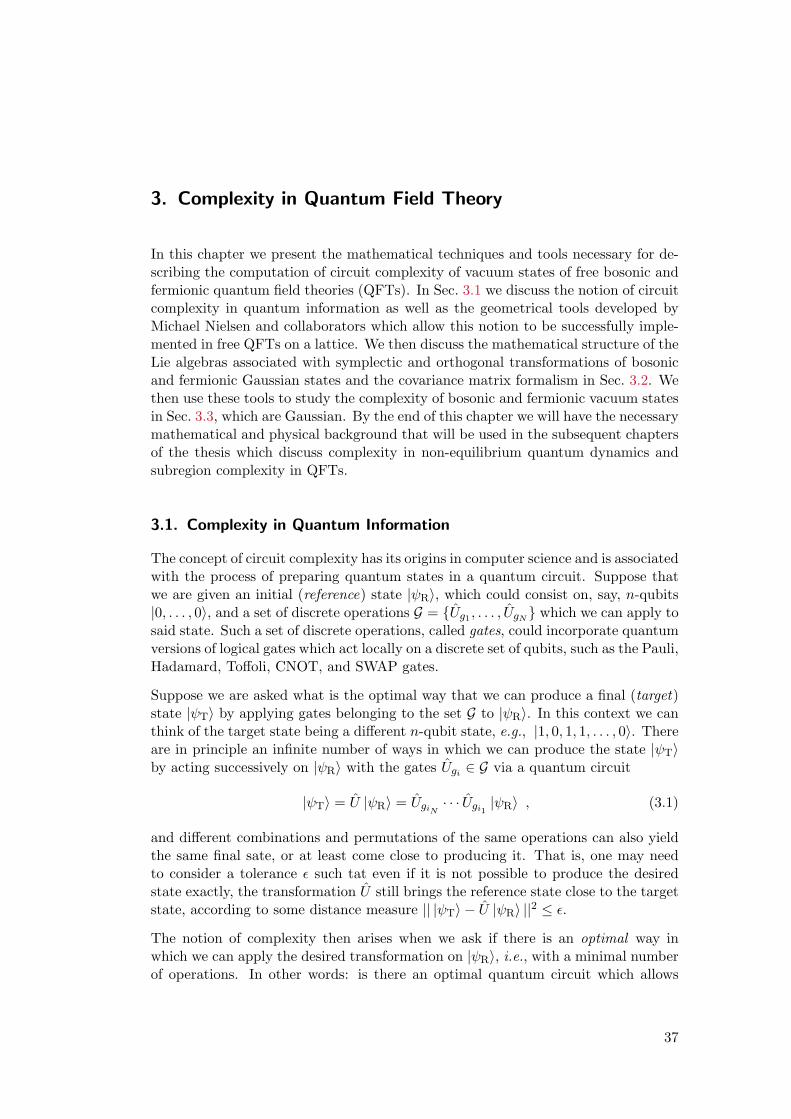
3. Complexity in Quantum Field Theory
In this chapter we present the mathematical techniques and tools necessary for de-scribing the computation of circuit complexity of vacuum states of free bosonic andfermionic quantum field theories (QFTs). In Sec. 3.1 we discuss the notion of circuitcomplexity in quantum information as well as the geometrical tools developed byMichael Nielsen and collaborators which allow this notion to be successfully imple-mented in free QFTs on a lattice. We then discuss the mathematical structure of theLie algebras associated with symplectic and orthogonal transformations of bosonicand fermionic Gaussian states and the covariance matrix formalism in Sec. 3.2. Wethen use these tools to study the complexity of bosonic and fermionic vacuum statesin Sec. 3.3, which are Gaussian. By the end of this chapter we will have the necessarymathematical and physical background that will be used in the subsequent chaptersof the thesis which discuss complexity in non-equilibrium quantum dynamics andsubregion complexity in QFTs.
3.1. Complexity in Quantum Information
The concept of circuit complexity has its origins in computer science and is associatedwith the process of preparing quantum states in a quantum circuit. Suppose thatwe are given an initial (reference) state | Ri, which could consist on, say, n-qubits|0, . . . , 0i, and a set of discrete operations G = Ug1 , . . . , UgN which we can apply tosaid state. Such a set of discrete operations, called gates, could incorporate quantumversions of logical gates which act locally on a discrete set of qubits, such as the Pauli,Hadamard, Toffoli, CNOT, and SWAP gates.
Suppose we are asked what is the optimal way that we can produce a final (target)state | Ti by applying gates belonging to the set G to | Ri. In this context we canthink of the target state being a different n-qubit state, e.g., |1, 0, 1, 1, . . . , 0i. Thereare in principle an infinite number of ways in which we can produce the state | Tiby acting successively on | Ri with the gates Ugi 2 G via a quantum circuit
| Ti = U | Ri = UgiN· · · Ugi1
| Ri , (3.1)
and different combinations and permutations of the same operations can also yieldthe same final sate, or at least come close to producing it. That is, one may needto consider a tolerance such tat even if it is not possible to produce the desiredstate exactly, the transformation U still brings the reference state close to the targetstate, according to some distance measure || | Ti U | Ri ||2 .
The notion of complexity then arises when we ask if there is an optimal way inwhich we can apply the desired transformation on | Ri, i.e., with a minimal numberof operations. In other words: is there an optimal quantum circuit which allows
37
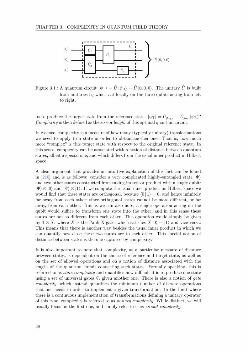
CHAPTER 3. COMPLEXITY IN QUANTUM FIELD THEORY
Figure 3.1.: A quantum circuit | Ti = U | Ri = U |0, 0, 0i. The unitary U is built
from unitaries Ui which act locally on the three qubits acting from leftto right.
us to produce the target state from the reference state: | Ti = UgαM· · · Ugα1
| Ri?Complexity is then defined as the size or length of this optimal quantum circuit.
In essence, complexity is a measure of how many (typically unitary) transformationswe need to apply to a state in order to obtain another one. That is, how muchmore “complex” is this target state with respect to the original reference state. Inthis sense, complexity can be associated with a notion of distance between quantumstates, albeit a special one, and which differs from the usual inner product in Hilbertspace.
A clear argument that provides an intuitive explanation of this fact can be foundin [210] and is as follows: consider a very complicated highly-entangled state |Ψiand two other states constructed from taking its tensor product with a single qubit:|Ψi |0i and |Ψi |1i. If we compute the usual inner product on Hilbert space wewould find that these states are orthogonal, because h0 | 1i = 0, and hence infinitelyfar away from each other; since orthogonal states cannot be more different, or faraway, from each other. But as we can also note, a single operation acting on thequbit would suffice to transform one state into the other; and in this sense thesestates are not so different from each other. This operation would simply be givenby 1 X, where X is the Pauli X-gate, which satisfies X |0i = |1i and vice versa.This means that there is another way besides the usual inner product in which wecan quantify how close these two states are to each other. This special notion ofdistance between states is the one captured by complexity.
It is also important to note that complexity, as a particular measure of distancebetween states, is dependent on the choice of reference and target state, as well ason the set of allowed operations and on a notion of distance associated with thelength of the quantum circuit connecting such states. Formally speaking, this isreferred to as state complexity and quantifies how difficult it is to produce one stateusing a set of universal gates G, given another one. There is also a notion of gatecomplexity, which instead quantifies the minimum number of discrete operationsthat one needs in order to implement a given transformation. In the limit wherethere is a continuous implementation of transformations defining a unitary operatorof this type, complexity is referred to as unitary complexity. While distinct, we willusually focus on the first one, and simply refer to it as circuit complexity.
38
3.1. COMPLEXITY IN QUANTUM INFORMATION
These are intimately connected with another concept commonly used in computerscience called computational complexity. This notion refers to the hardness of com-putational problems and is often formalized in terms of number of steps required bydeterministic Turing machines to solve given computational problems [28, 211, 212].In computational complexity theory one studies different classes of promise prob-lems and attempts to classify whether they are solvable and under which conditions.While this concept does not enter the main discussion of this work, it is still relevantto establish a connection between the notion of complexity that we are interestedin, and other ones which are also used in computer science, and which are centralto the efforts of realizing quantum computers.
Coming back to quantum circuits such as (3.1), it’s not too difficult to convinceoneself that it is in general a complicated question to ask what is the optimal choiceof gates that produces a desired target state. Or what is the most efficient way toimplement a desired operation on a given reference state. This is in fact a centralproblem of quantum computing and apart from certain known examples, it is ingeneral not known how to efficiently, i.e., in polynomial time, implement unitaryoperations on quantum systems comprised of many qubits.
3.1.1. The Geometric Approach to Circuit Complexity
It is because of this, that the ideas developed by Michael Nielsen and collaboratorson how to tackle the construction of quantum circuits using geometric tools [213–215] became relevant and even crossed the border of quantum computing and intothe high-energy physics community. Over such series of works, they systematicallytranslated the problem of finding optimal quantum circuits that efficiently imple-ment a unitary operation U , into the problem of finding geodesics in Riemannianmanifolds. Initially Nielsen intended his computations to serve as a lower bound onthe minimal size of a quantum circuit that exactly implements an n-qubit operation,as can be seen in [214].
In order to do this, they used the theory of optimal quantum control [216–218] toconstruct a time-dependent Hamiltonian H(t) that generates the desired unitary Uin (3.1) via
U = P
exp
i
Z 1
0dt H(t)
, (3.2)
where the control Hamiltonian H(t) is expanded in terms of elementary operationsKI as
1
H(t) =X
I
Y I(t)KI , (3.3)
where the symbol P in (3.2) denotes a path-ordering such that the operations at
earlier time-steps are applied to the reference state first, i.e., the quantum circuitis built from right to left. The Y I(t) are control functions which are responsible for
1In Nielsen’s original works the elementary operations KI corresponded to Pauli matrices, giventhat he was interested in studying the action of SU(2n) gates on quantum circuits comprised ofn-qubit states.
39
CHAPTER 3. COMPLEXITY IN QUANTUM FIELD THEORY
“activating” a particular gate KI at time t. Note that in order for U in (3.2) to beunitary, the generators KI in (3.3) must be Hermitian.
Note that (3.2) defines path in the space of unitaries G via
U() = P
exp
i
Z τ
0dt H(t)
, (3.4)
with boundary conditions: U( = 1) = U , as in (3.2), and U( = 0) = 1. Then,for every value of 2 [0, 1], the action of the unitary U() on the reference state| Ri defines a state | ()i which is constructed from the successive application ofgates KI activated by functions Y I(t). From (3.4) we can also see that the controlfunctions Y I define in general a tangent vector to the trajectory U() with
X
I
Y I()KI =dU()
dU1() . (3.5)
The idea is then to associate a cost for different circuits associated with paths inHilbert space defined by unitaries (3.4). This is done by considering a cost functionF (U(), @τ U()), such that
DF (U) =
Z 1
0d F (U(), @τ U()) , (3.6)
defines the depth, or length lF (U), of the circuit. In order to identify the optimalcircuit one should find the minimum of DF (U) for a choice of cost function F .
The authors of [213–215] identified the properties that cost functions F (U, v) withU 2 G and v 2 TU (G) should have in order to by physically reasonable. Theseproperties include continuity, positivity, (positive) homogeneity and subadditivity.If one further imposes the condition of smoothness, then (3.6) defines a distanceor length functional for a class of smooth manifolds called Finsler manifolds [219].Essentially, a Finsler manifold is a manifold where each tangent space is equippedwith a norm that is not necessarily induced by an inner product.
In such a way, the authors of [213–215] translated the problem of finding optimalcircuits into the problem of finding geodesics in Finsler geometries, where the com-plexity of the circuit is identified with the length of the geodesic joining the referenceand target states. In other words
CF := min[DF ] . (3.7)
Regarding the cost functions F (3.6), the authors of [213–215] the properties ofpossibilities such as
F p1 (U,
~Y ) =X
I
pI(U)Y I
, (3.8a)
F q2 (U,
~Y ) =
sX
IJ
qIJ(U)Y IY J , (3.8b)
where the functions pI(U), qIJ(U) are penalty factors, i.e., numbers or functionswhich are meant to penalize certain functions Y I in order to control how much
40
3.2. GAUSSIAN TECHNIQUES
a particular operator KI contributes to the circuit depth at given points of thepath U() thus providing a way of distinguishing between gates which are “easy”to implement, and gates which are “hard” to implement. That is, penalty factorsare used to “penalize” certain gates in the quantum circuit. In the case in whichthere are no penalty factors, i.e., pI / 1 and qIJ / 12, these cost functions aresimply denoted respectively by F1 and F2, and define the known L1 and L2 normsin finite-dimensional vector spaces.
The authors of [213–215] were particularly interested in the first one of these,namely (3.8a), since its associated circuit depth (3.6) can be interpreted as thetime needed to implement the unitary (3.4). However its main disadvantage is thatit is not smooth. As a consequence, the cost function (3.8a) does not define aFinsler metric and one cannot directly apply the calculus of variations to find itsminimal-length curves. In other words, minimizing such cost function is in generala challenging task.
This is not the case for (3.8b). Here, the positive-definite functions qIJ(U) can bethought of as defining a local metric on the tangent space TY (U). In this sense, thiscost function induces the known L2-type norm or distance, used to characterize thelength of curves in Riemannian geometry, and which allows for a minimization ofthe circuit depth D2 (3.6) using the known techniques of calculus of variations anddifferential geometry.
Apart from these two, one could in principle consider other cost functions whichincorporate sums of products of p control functions with an appropriate power of1/p. Such functions would be of the form Fp (
PI |Y
I|p)1/p and would lead to Lp
norms. While mathematically interesting, these kinds of norms are less studied inthe context of complexity.
Even though in the context of [213–215] only the F1 cost function appeared to haveinteresting properties, it is a priori not clear which one of these would be “appro-priate” in a different scenario. Of course, the advantage of the F2 cost function isthat it is in principle possible to minimize its associated circuit depth D2, while thephysical interpretation of the F1 cost function is closer to the original motivationof understanding how to efficiently implement an n-qubit operation as in the caseof [213–215]. As we will see in Sec. 3.3.1 and Sec. 3.3.2, the geometric approachput forth by the authors of [213–215] will allow us to study the complexity of va-cuum states of free quantum field theories. In these cases, the spaces of unitarieswill consist of symplectic and orthogonal transformations allowing for an elegantdescription using the covariance matrix formalism, which will be the focus of thefollowing section.
3.2. Gaussian Techniques
Given a quantum field theory (QFT) in D-dimensions, one is typically interestedin computing n-point correlation functions, such as h0|O1(x1) · · · On(xn)|0i for a setof operators Oi associated with physical observables, as these are directly relatedto the probability amplitude of physical processes in said theory. In momentum
41
CHAPTER 3. COMPLEXITY IN QUANTUM FIELD THEORY
space, such correlators give rise to scattering amplitudes which yield the probabilityamplitude of scattering processes of particles in the theory.
In essence, knowing the n-point correlation functions of a state in a quantum fieldtheory amounts to having access to all its relevant physical information. However, itis in practice a difficult task to actually compute these n-point functions, althoughcrucial results such as Wick’s theorem allows us to reduce the problem of computinghigher-point functions to lower-point functions. At the same time, in conformal fieldtheories in D-dimensions, two and three-point functions of primary fields are com-pletely fixed, up to normalization, by conformal symmetry [220]. In contrast, higher-point functions are not fully determined by conformal symmetry and are in generalfunctions of cross-ratios of spacetime coordinates and are theory-dependent.
The choice of a quantum state is also implicit in the computation of the correlationfunctions. Typically one considers ground states of free theories or primary statesin the case of conformal field theories. Of special interest in this work, however, arethe ground states of free Hamiltonians in quantum field theories, as these have theproperty of being completely characterised by their two-point functions. While atfirst glance this fact could be interpreted as signaling the mathematical triviality ofsuch states, they are in fact used extensively in quantum information and quantumfield theory. The fact that Gaussian states are completely characterized by theirtwo-point functions also allows us to use the mathematical machinery of symplecticand orthogonal transformations and their associated Lie groups to describe them. Aswe will show in the following chapters, this will in turn allow to study the complexityand entanglement of vacuum states of free quantum field theories in a compact andelegant way, providing also a clear picture of how the physical information of suchstates is encoded in these quantities.
3.2.1. The Covariance Matrix Approach
In the following sections and chapters, we will be interested in studying the com-plexity of Gaussian states in free bosonic QFTs on a lattice. As a consequence, itwill be useful to have a complete description of their mathematical properties. Wewill do this in this section.
A bosonic or fermionic system with N degrees of freedom can be described by 2Nobservables a q1, p1, . . . , qN , pN which correspond to canonical coordinates in aclassical phase space. Such phase space coordinates satisfy canonical commutationor anticommutation relations
[a, b] = iΩab , (3.9a)
a, b = Gab , (3.9b)
where Gab is a symmetric positive definite metric and Ωab is a non-degenerate anti-
symmetric symplectic form.
A normalized Gaussian quantum state | i with vanishing one-point functions h |a| i =0 is completely characterised by its two-point function Cab
2 with entries definedby
Cab2 := h | ab | i . (3.10)
42
3.2. GAUSSIAN TECHNIQUES
We can also decompose it into a symmetric and an antisymmetric part
Cab2 =
1
2
Gab + iΩab
. (3.11)
It can be shown that due to the commutation and anticommutation relations (3.9)and up to basis’ transformations, Gab is fixed for fermions while Ω
ab is fixed forbosons, which implies that only the other piece of the two-point function (3.11),namely Gab for bosons and Ω
ab for fermions, will depend on the state | i. By thiswe mean that for a given choice of basis a, the expressions for Ω
ab and Gab arefixed. For example, in canonical coordinates a = (q1, p1, . . . , qN , pN )
Ω =
0 1N
1N 0
, G =
1N 00 1N
, (3.12)
where 1N is the identity matrix in N dimensions. As a consequence, Ωab and Gab
completely characterize Gaussian states and are respectively called the fermionicand bosonic covariance matrices.
Consider, for example, a pure Gaussian state | i corresponding to the ground state ofa single harmonic oscillator in a bosonic free quantum field theory, i.e., | i describesa single bosonic mode. Such a state can be characterized by its wavefunction
hq| i = (q) =a
1/4exp
1
2(a+ ib)q2
, (3.13)
where a, b 2 R, and a > 0. In this case, the covariance matrix
Gab := h | (ab + ba) | i , (3.14)
can be computed directly using canonical coordinates a = q, p and is givenby
G =
1a
ba
ba
a2+b2
a
. (3.15)
In the wavefunction (3.13), the functions a and b completely characterize the Gaus-sian state. Equivalently, one can think of these as given in terms of the covariancematrix entries (3.15), which are related to the 2-point correlation functions via
a =1
G11=
1
h | 2q2 | i , (3.16a)
b =G21
G11=h | (qp+ pq) | ih | 2q2 | i , (3.16b)
where G11 = h | 2q2 | i > 0, thus showing that the covariance matrix (3.15) containsthe same physical information about the state as the wavefunction (3.13). Thereare other equivalent ways of representing Gaussian states which are not coveredin this present work, such as the characteristic function and the quasi-probabilitydistribution. The reader can refer to [221] for a detailed description of them.
One can further check that in this case det(G) = 1 and therefore the entry G22
of (3.15) doesn’t carry additional information about the state. The fact that the
43
CHAPTER 3. COMPLEXITY IN QUANTUM FIELD THEORY
determinant of the covariance matrix of state (3.13) is the unity is a general propertyof pure Gaussian states.
This can be made more precise by the definition of a linear map called the linearcomplex structure Jab defined via
Jab := Gac
Ω1cb = Ω
acG1cb . (3.17)
It can be shown that | i is a pure Gaussian state, if and only if J2 = 1, whichimplies that the eigenvalues of J , called symplectic eigenvalues, which in generalcome in pairs, are given in this case by ±i [222, 223].
It is also important to note that the complex structure J provides a unified way ofdenoting both bosonic and fermionic Gaussian states simply by |Ji, as it integratesboth the symmetric and antisymmetric part of the 2-point function (3.11). It alsoallows to define a notion of creation and annihilation operators [224] and on themathematical level, it endows the phase space of Gaussian states with a Kaler struc-ture, a full description of which escapes the scope of this work. However, the readercan refer to the elegant discussion of this aspect of Gaussian states in [221].
Of course, not only pure Gaussian states can be described in terms of their complexlinear structure. Mixed Gaussian states described by a density matrix are alsouniquely characterized by their covariance matrix, computed in this case via
Gabρ = tr
ab + ba
, (3.18a)
Ωabρ = tr
ab ba
, (3.18b)
in which case, their complex structures now satisfies the inequalities: 1 J2 forbosons, and 0 J2 1 for fermions. Additionally, in order for a mixed state tobe Gaussian, there should exist a positive-definite bilinear form qab and a constantc0 such that
=
(eqabξ
aξbc0 ,
ei qabξaξbc0 ,
(3.19)
where the top expression corresponds to bosons, and the bottom one to fermions. Wewill return to mixed Gaussian states when we discuss complexity and entanglementof purification, in Ch. 5 and 6.
3.2.2. The Symplectic and Orthogonal Groups
The usefulness of the covariance matrix approach, however, becomes manifest whenone studies trajectories of states within the subspace of Gaussian states. By con-sidering only such a class of states one gets restricted to transformations belongingto the symplectic group Sp(2N,R) in the case of bosons, and to the orthogonalgroup O(2N,R) in the case of fermions. The reason being that these Lie groupspreserve the symplectic form Ω
ab and the metric Gab respectively, allowing us to re-main within the subspace of Gaussian states. These Lie groups are formally definedin the following way
Sp(2N,R) := Mab 2 GL(2N,R) |MΩM| = Ω , (3.20a)
44
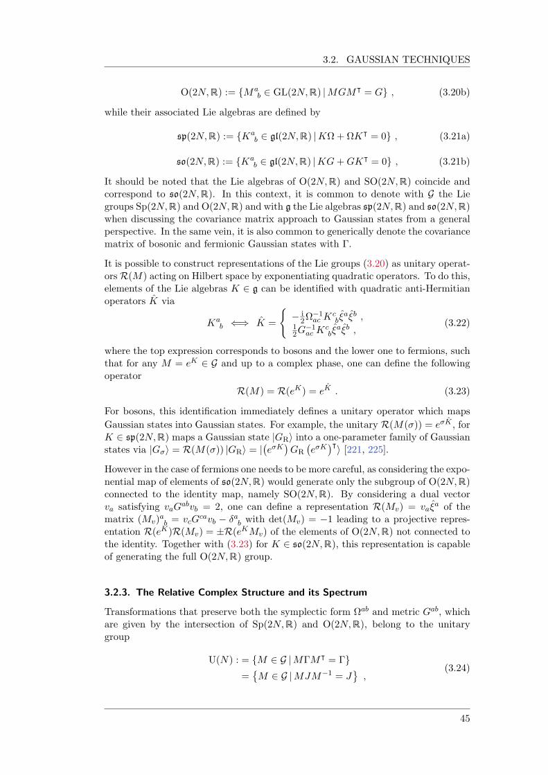
3.2. GAUSSIAN TECHNIQUES
O(2N,R) := Mab 2 GL(2N,R) |MGM| = G , (3.20b)
while their associated Lie algebras are defined by
sp(2N,R) := Kab 2 gl(2N,R) |KΩ+ ΩK| = 0 , (3.21a)
so(2N,R) := Kab 2 gl(2N,R) |KG+GK| = 0 , (3.21b)
It should be noted that the Lie algebras of O(2N,R) and SO(2N,R) coincide andcorrespond to so(2N,R). In this context, it is common to denote with G the Liegroups Sp(2N,R) and O(2N,R) and with g the Lie algebras sp(2N,R) and so(2N,R)when discussing the covariance matrix approach to Gaussian states from a generalperspective. In the same vein, it is also common to generically denote the covariancematrix of bosonic and fermionic Gaussian states with Γ.
It is possible to construct representations of the Lie groups (3.20) as unitary operat-orsR(M) acting on Hilbert space by exponentiating quadratic operators. To do this,elements of the Lie algebras K 2 g can be identified with quadratic anti-Hermitianoperators K via
Kab () K =
( i
2Ω1ac K
cb
ab ,12G
1ac K
cb
ab ,(3.22)
where the top expression corresponds to bosons and the lower one to fermions, suchthat for any M = eK 2 G and up to a complex phase, one can define the followingoperator
R(M) = R(eK) = eK . (3.23)
For bosons, this identification immediately defines a unitary operator which maps
Gaussian states into Gaussian states. For example, the unitary R(M()) = eσK , forK 2 sp(2N,R) maps a Gaussian state |GRi into a one-parameter family of Gaussianstates via |Gσi = R(M()) |GRi = |
eσK
GR
eσK
|i [221, 225].
However in the case of fermions one needs to be more careful, as considering the expo-nential map of elements of so(2N,R) would generate only the subgroup of O(2N,R)connected to the identity map, namely SO(2N,R). By considering a dual vectorva satisfying vaG
abvb = 2, one can define a representation R(Mv) = vaa of the
matrix (Mv)ab = vcG
cavb ab with det(Mv) = 1 leading to a projective repres-entation R(eK)R(Mv) = ±R(eKMv) of the elements of O(2N,R) not connected tothe identity. Together with (3.23) for K 2 so(2N,R), this representation is capableof generating the full O(2N,R) group.
3.2.3. The Relative Complex Structure and its Spectrum
Transformations that preserve both the symplectic form Ωab and metric Gab, which
are given by the intersection of Sp(2N,R) and O(2N,R), belong to the unitarygroup
U(N) : = M 2 G |MΓM| = Γ
=M 2 G |MJM1 = J
,
(3.24)
45
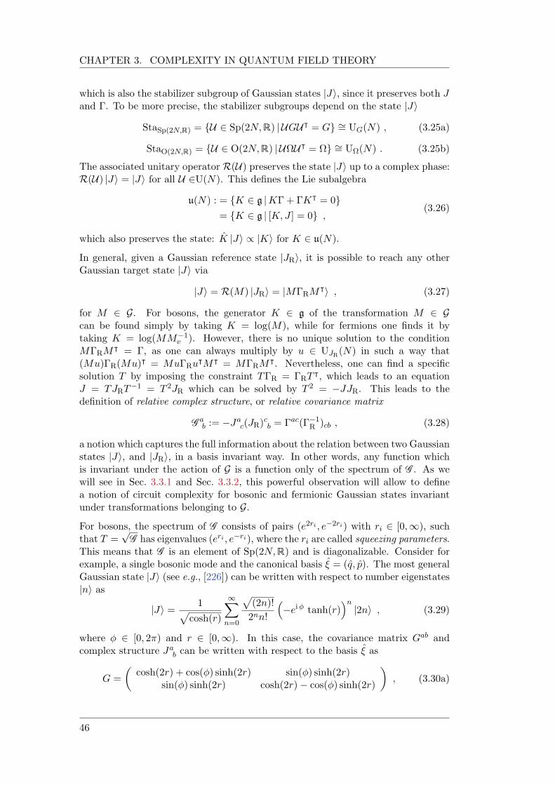
CHAPTER 3. COMPLEXITY IN QUANTUM FIELD THEORY
which is also the stabilizer subgroup of Gaussian states |Ji, since it preserves both Jand Γ. To be more precise, the stabilizer subgroups depend on the state |Ji
StaSp(2N,R) = U 2 Sp(2N,R) | UGU| = G = UG(N) , (3.25a)
StaO(2N,R) = U 2 O(2N,R) | UΩU| = Ω = UΩ(N) . (3.25b)
The associated unitary operator R(U) preserves the state |Ji up to a complex phase:R(U) |Ji = |Ji for all U 2U(N). This defines the Lie subalgebra
u(N) : = K 2 g |KΓ+ ΓK| = 0
= K 2 g | [K, J ] = 0 ,(3.26)
which also preserves the state: K |Ji / |Ki for K 2 u(N).
In general, given a Gaussian reference state |JRi, it is possible to reach any otherGaussian target state |Ji via
|Ji = R(M) |JRi = |MΓRM|i , (3.27)
for M 2 G. For bosons, the generator K 2 g of the transformation M 2 Gcan be found simply by taking K = log(M), while for fermions one finds it bytaking K = log(MM1
v ). However, there is no unique solution to the conditionMΓRM
| = Γ, as one can always multiply by u 2 UJR(N) in such a way that(Mu)ΓR(Mu)| = MuΓRu
|M| = MΓRM|. Nevertheless, one can find a specific
solution T by imposing the constraint TΓR = ΓRT|, which leads to an equation
J = TJRT1 = T 2JR which can be solved by T 2 = JJR. This leads to the
definition of relative complex structure, or relative covariance matrix
Gab := Ja
c(JR)cb = Γ
ac(Γ1R )cb , (3.28)
a notion which captures the full information about the relation between two Gaussianstates |Ji, and |JRi, in a basis invariant way. In other words, any function whichis invariant under the action of G is a function only of the spectrum of G . As wewill see in Sec. 3.3.1 and Sec. 3.3.2, this powerful observation will allow to definea notion of circuit complexity for bosonic and fermionic Gaussian states invariantunder transformations belonging to G.
For bosons, the spectrum of G consists of pairs (e2ri , e2ri) with ri 2 [0,1), suchthat T =
pG has eigenvalues (eri , eri), where the ri are called squeezing parameters.
This means that G is an element of Sp(2N,R) and is diagonalizable. Consider forexample, a single bosonic mode and the canonical basis = (q, p). The most generalGaussian state |Ji (see e.g., [226]) can be written with respect to number eigenstates|ni as
|Ji = 1pcosh(r)
1X
n=0
p(2n)!
2nn!
eiφ tanh(r)
n|2ni , (3.29)
where 2 [0, 2) and r 2 [0,1). In this case, the covariance matrix Gab andcomplex structure Ja
b can be written with respect to the basis as
G =
cosh(2r) + cos() sinh(2r) sin() sinh(2r)
sin() sinh(2r) cosh(2r) cos() sinh(2r)
, (3.30a)
46
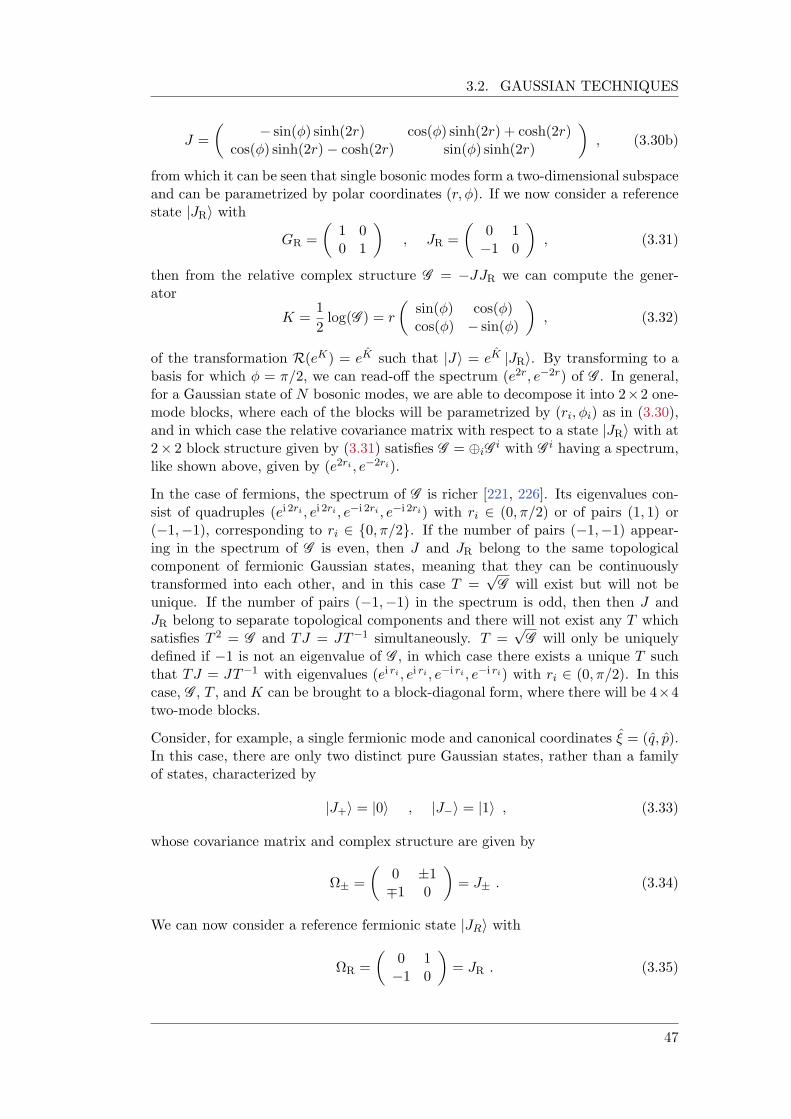
3.2. GAUSSIAN TECHNIQUES
J =
sin() sinh(2r) cos() sinh(2r) + cosh(2r)
cos() sinh(2r) cosh(2r) sin() sinh(2r)
, (3.30b)
from which it can be seen that single bosonic modes form a two-dimensional subspaceand can be parametrized by polar coordinates (r,). If we now consider a referencestate |JRi with
GR =
1 00 1
, JR =
0 11 0
, (3.31)
then from the relative complex structure G = JJR we can compute the gener-ator
K =1
2log(G ) = r
sin() cos()cos() sin()
, (3.32)
of the transformation R(eK) = eK such that |Ji = eK |JRi. By transforming to abasis for which = /2, we can read-off the spectrum (e2r, e2r) of G . In general,for a Gaussian state of N bosonic modes, we are able to decompose it into 22 one-mode blocks, where each of the blocks will be parametrized by (ri,i) as in (3.30),and in which case the relative covariance matrix with respect to a state |JRi with at2 2 block structure given by (3.31) satisfies G = iG
i with G i having a spectrum,like shown above, given by (e2ri , e2ri).
In the case of fermions, the spectrum of G is richer [221, 226]. Its eigenvalues con-sist of quadruples (ei 2ri , ei 2ri , ei 2ri , ei 2ri) with ri 2 (0,/2) or of pairs (1, 1) or(1,1), corresponding to ri 2 0,/2. If the number of pairs (1,1) appear-ing in the spectrum of G is even, then J and JR belong to the same topologicalcomponent of fermionic Gaussian states, meaning that they can be continuouslytransformed into each other, and in this case T =
pG will exist but will not be
unique. If the number of pairs (1,1) in the spectrum is odd, then then J andJR belong to separate topological components and there will not exist any T whichsatisfies T 2 = G and TJ = JT1 simultaneously. T =
pG will only be uniquely
defined if 1 is not an eigenvalue of G , in which case there exists a unique T suchthat TJ = JT1 with eigenvalues (ei ri , ei ri , ei ri , ei ri) with ri 2 (0,/2). In thiscase, G , T , and K can be brought to a block-diagonal form, where there will be 44two-mode blocks.
Consider, for example, a single fermionic mode and canonical coordinates = (q, p).In this case, there are only two distinct pure Gaussian states, rather than a familyof states, characterized by
|J+i = |0i , |Ji = |1i , (3.33)
whose covariance matrix and complex structure are given by
Ω± =
0 ±11 0
= J± . (3.34)
We can now consider a reference fermionic state |JRi with
ΩR =
0 11 0
= JR . (3.35)
47
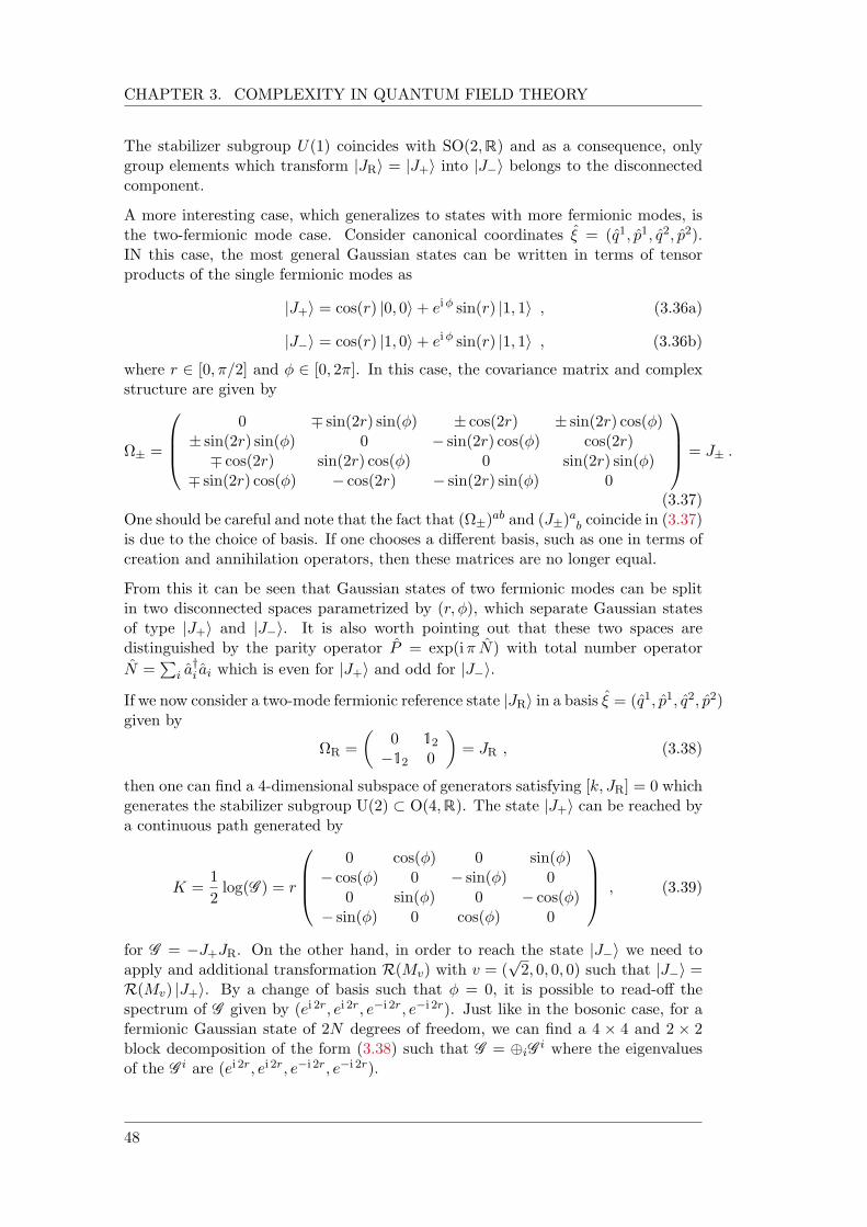
CHAPTER 3. COMPLEXITY IN QUANTUM FIELD THEORY
The stabilizer subgroup U(1) coincides with SO(2,R) and as a consequence, onlygroup elements which transform |JRi = |J+i into |Ji belongs to the disconnectedcomponent.
A more interesting case, which generalizes to states with more fermionic modes, isthe two-fermionic mode case. Consider canonical coordinates = (q1, p1, q2, p2).IN this case, the most general Gaussian states can be written in terms of tensorproducts of the single fermionic modes as
|J+i = cos(r) |0, 0i+ eiφ sin(r) |1, 1i , (3.36a)
|Ji = cos(r) |1, 0i+ eiφ sin(r) |1, 1i , (3.36b)
where r 2 [0,/2] and 2 [0, 2]. In this case, the covariance matrix and complexstructure are given by
Ω± =
0BB@
0 sin(2r) sin() ± cos(2r) ± sin(2r) cos()± sin(2r) sin() 0 sin(2r) cos() cos(2r) cos(2r) sin(2r) cos() 0 sin(2r) sin()
sin(2r) cos() cos(2r) sin(2r) sin() 0
1CCA = J± .
(3.37)One should be careful and note that the fact that (Ω±)
ab and (J±)ab coincide in (3.37)
is due to the choice of basis. If one chooses a different basis, such as one in terms ofcreation and annihilation operators, then these matrices are no longer equal.
From this it can be seen that Gaussian states of two fermionic modes can be splitin two disconnected spaces parametrized by (r,), which separate Gaussian statesof type |J+i and |Ji. It is also worth pointing out that these two spaces aredistinguished by the parity operator P = exp(i N) with total number operator
N =P
i a†i ai which is even for |J+i and odd for |Ji.
If we now consider a two-mode fermionic reference state |JRi in a basis = (q1, p1, q2, p2)given by
ΩR =
0 12
12 0
= JR , (3.38)
then one can find a 4-dimensional subspace of generators satisfying [k, JR] = 0 whichgenerates the stabilizer subgroup U(2) O(4,R). The state |J+i can be reached bya continuous path generated by
K =1
2log(G ) = r
0BB@
0 cos() 0 sin() cos() 0 sin() 0
0 sin() 0 cos() sin() 0 cos() 0
1CCA , (3.39)
for G = J+JR. On the other hand, in order to reach the state |Ji we need toapply and additional transformation R(Mv) with v = (
p2, 0, 0, 0) such that |Ji =
R(Mv) |J+i. By a change of basis such that = 0, it is possible to read-off thespectrum of G given by (ei 2r, ei 2r, ei 2r, ei 2r). Just like in the bosonic case, for afermionic Gaussian state of 2N degrees of freedom, we can find a 4 4 and 2 2block decomposition of the form (3.38) such that G = iG
i where the eigenvaluesof the G i are (ei 2r, ei 2r, ei 2r, ei 2r).
48
3.3. COMPLEXITY IN QUANTUM FIELD THEORIES
3.3. Complexity in Quantum Field Theories
The holographic complexity proposals discussed in Sec. 2.3 raised a challenge on ourunderstanding the black hole interior, provided a definition of its volume in a covari-ant way and made a conjecture relating it to complexity, opening a new perspectiveinto the study of the holographic black holes. The fact that these gravitationalquantities capable of probing the interior of AdS black holes are conjectured to berelated to the difficulty of preparing states in chaotic quantum many-body systemsprovides another prime example of how deeply intertwined ideas from quantum in-formation are with gravity in negatively curved spaces.
Of course, the prototypical example of this intimate relation between quantum in-formation and gravity is encapsulated by the notion of entanglement entropy, whichhas played a key role in the development of the field over the past fifteen years. TheRyu–Takayanagi formula [118, 227], discussed in Sec. 2.1.1, and its covariant general-ization [123] provided a stepping stone for understanding the way that gravitationalquantities are encoded in the boundary quantum field theories.
However a key aspect of the development of the study of entanglement entropy inholographic theories, and particularly in the AdS/CFT correspondence, is that priorto the Ryu–Takayanagi conjecture in the AdS/CFT Correspondence, the concept ofentanglement entropy had already been established in quantum field theories bypioneering works such as [109, 111] (see Sec. 2.1 for more details). Afterwards andthrough a series of pivotal works [127, 128, 132, 138, 228, 229] the validity of theduality of descriptions of entanglement entropy was strengthened. One could evenargue that a significant amount of the “success” of the Ryu–Takayanagi formula isdue to the possibility of matching its predictions from both sides of the holographicduality.
In stark contrast, the notion of complexity in the AdS/CFT correspondence enteredthrough the holographic proposals (see Sec. 2.3.1 and Sec. 2.3.2) without a preex-isting notion of complexity in quantum field theory. While the arguments in theoriginal holographic proposals [170, 173, 178, 179] indeed connect a notion of com-plexity arising from tensor network arguments with such gravitational observables,the lack of a concrete definition of it on the quantum field theory side hinders thepossibility of reconciling their proposals with any computation of complexity arisingfrom first-principles.
As a consequence of this, a significant amount of effort in the community over thepast five years has been devoted to bringing the notion of complexity on a similarfooting to entanglement entropy in quantum field theories. Two fundamental worksin this direction [101, 102] were inspired by the geometric approach developed byauthors of [213–215] (see Sec. 3.1.1) and by the continuous multi-scale entanglementrenormalization ansatz (cMERA) [95] (see Sec. 1.2). The first of these relied on alattice approach to study the complexity of the vacuum state of a free scalar fieldtheory, where the measure of complexity was defined via the geodesic distance ofa Riemannian metric defined through the generators of unitaries belonging to thegeneral linear group GL(N,R), in a manner akin to the geometric approach. Thesecond one was based on the cMERA approach to quantum field theories, and the
49
CHAPTER 3. COMPLEXITY IN QUANTUM FIELD THEORY
authors obtained complexity as a geodesic distance of the Fubini-Study metric forthe SU(1, 1)N group of Gaussian states generated by the action of this group.
In a subsequent works such techniques were applied to study the circuit complexityof free fermions [204] with an approach based on the notion of geodesic distance onthe SO(2N,R) group. One should also mention [205], where the cMERA approachwas used to study complexity once again in fermionic field theories. Similar methodshave also been applied in other relevant set-ups, such as thermofield double (TDF)states [230] and conformal field theories [206, 208, 209, 231].
In this section we review the construction and results for circuit complexity for thevacuum states of two free quantum field theories in (1 + 1)-dimensions: the Klein–Gordon field and the critical transverse field Ising model. This section lays thefoundation for subsequent chapters in this thesis, in particular to Chap 5, where wediscuss a notion of complexity for mixed states called complexity of purification. Atthe same time, the models that we are considering will also appear in Chap 4 wherewe study the time-dependence of complexity and also in Chap 6 where we insteadstudy entanglement of purification and reflected entropy.
Vacuum states of two free quantum field theories in (1 + 1)-dimensions have theproperty of being Gaussian and we will hence be able to use the machinery describedin Sec. 3.2 to study the complexity of their vacuum states. In order to regularize theUV divergences, we will consider lattice representations of such theories, even thoughone could also regularise it by placing a cut-off ΛUV in momentum space.
The approach that we will follow is based on the geometrization of complexity asdescribed in Sec. 3.1.1 where circuits are built from a continuous representationof unitaries, which in the case of bosons will correspond to unitaries built fromsymplectic transformations and for fermions from orthogonal ones. Furthermore, wewill focus on the F2 cost function (3.8b) as derived originally in [204, 230], whichis based on a natural metric on the group manifold and which coincides with thegeodesic distance on the Gaussian state manifold, i.e., with the Fubini-Study metric,studied originally in [101]. The main reason for this is that such cost function allowsfor an analytical minimization, in contrast with other cost functions, such as F1. Oneshould mention, nonetheless, that the latter one is expected to have properties whichmore closely resemble the holographic complexity proposals. The following sectionswill also serve as the basis for the content of chapters 4 and 5, where we will studycomplexity in the context of quantum quenches and complexity of purification.
3.3.1. Complexity of the Klein–Gordon Vacuum
Consider the Hamiltonian of a free massive scalar field in (1 + 1)- spacetime dimen-sions
H =1
2
Zdx
(x)2 + '0(x)2 +m2'(x)2
, (3.40)
where '(x) and (x) are the field and conjugate momentum operators, respectively.This theory describes the well known Klein–Gordon field with mass m.
We now introduce a lattice spacing and discretize the Hamiltonian (3.40) on a
50
3.3. COMPLEXITY IN QUANTUM FIELD THEORIES
circular lattice with N sites and circumference L = N
H =
2
N1X
i=0
2i +
m2
2'2i +
1
4('i 'i+1)
2
, (3.41)
where 'i := '(xi) and i := (xi) correspond to our choice of canonical variablesai = ('i, i), and where a = 1, 2. Positions xi label the lattice site i, with i 20, . . . , N 1 with periodic boundary condition: xN+i = xi 8 i.The Hamiltonian (3.41) can be diagonalized via a discrete Fourier transform
'j =1pN
N1X
k=0
exp (2i k j/N) 'k , (3.42a)
j =1pN
N1X
k=0
exp (2i k j/N) k , (3.42b)
leading to
H =1
2
N1X
k=0
|k|
2 +!2k
|'k|
2
, (3.43)
which describes a system of N decoupled harmonic oscillators with frequencies
!k =
sm2 +
4
2sin2
k
N
. (3.44)
The ground state |0i of the Hamiltonian (3.43) is Gaussian, and hence fully charac-terized by its covariance matrix (3.14), written in a momentum basis ai = ('k, k)as
Gabij : = h | (ab + ba) | i
=1
N
N1X
k=0
ei2πkN
(ij)
1ωk
0
0 !k
,
(3.45)
where a, b labels the entries of Gij for sites i and j of the lattice. Note that the fullcovariance matrix can be decomposed in 2 2 blocks
G =N1M
k=0
1ωk
0
0 !k
=
N1M
k=0
Gk , (3.46)
which is just a consequence of the fact that we have decoupled the system by per-forming a normal mode decomposition.
Considering the continuum limit on a circle of circumference L = N requires totake the limit N !1 while keeping the product of meaningful combinations such asmL = mN fixed. Strictly speaking, each value of this combination corresponds toa different QFT in the continuum limit within the class of Klein–Gordon theories.In Chap. 5 we will be interested in considering subsystems and in this case thecontinuum limit will further require that as N is increased, quantities such as the
51
CHAPTER 3. COMPLEXITY IN QUANTUM FIELD THEORY
mutual information stabilize to a value in the vicinity of their QFT expectations. Ifw is the size of the subsystem, then the results of numerical computations shouldbe indistinguishable from the set-up when the spatial direction is a line. In thiscase, the mass of the field m 1/ becomes the only dimensionful parameter of thetheory in the continuum limit. Furthermore, in this case the discrete k associatedwith different momentum modes in (3.44) become a continuum variable and thediscrete sum in (3.45) must be replaced by an integral.
Before proceeding to the discussion of the reference state and complexity, it is worthpointing out a known subtlety of this discretized model, namely the zero-mode prob-lem: The frequency of the oscillator with zero momentum mode k = 0 is given by!0 = m, which vanishes in the massless limit m ! 0. This entails a divergence ofthe '' two-point function
h0|'0(xi)'0(xj)|0i 1
m
m!0!1 , (3.47)
leading to divergences in the covariance matrix (3.45), implying that in this limitthe ground state |0i approaches a delta distribution. This means that in this limitthe ground state of the theory (3.43) is only defined distributionally, and does notlie in Hilbert space, since it is not square integrable, i.e., it is not in L2(C).
If there is a problem with the zero-mode in the massless limit, then why bothertaking it at all? Because the massless limit of the Klein–Gordon model (3.40) is afree conformal field theory in (1 + 1)-dimensions with central charge c = 1, and itwill be the focus of Sec. 5.2.2.
To be precise, the c = 1 CFT with the periodic boundary conditions that we im-posed previously can be regarded as a 1-parameter family of theories which arisein the path-integral language from the compactification of the bosonic field ' withperiodicity
'+ 2R = ' , (3.48)
where R here is a dimensionless parameter corresponding to the compactificationradius in field space and that plays the role of a moduli which specifies a particularc = 1 CFT [232]. In this case, the scaling dimension of the lowest lying operator isgiven by
∆min = min
1
R2,R2
4
. (3.49)
Note that this expression is the same for a theory with a compactification radiusgiven by 2/R, which shows an underlying duality between theories with compatific-ation radii R and 2/R [232].
The massless limit of the discretized Klein–Gordon theory (3.41) corresponds tothe decompactification limit, R ! 1 of free compact bosonic CFTs, which as wejust mentioned, is a subtle limit since in this case the gap in the operator spectrumapproaches zero (3.49). This limit leads to the correct correlation functions of vertexoperators and single interval entanglement entropy. However, for other quantitiesthis limit is more complicated. Particularly for the partition function of the theory.
52
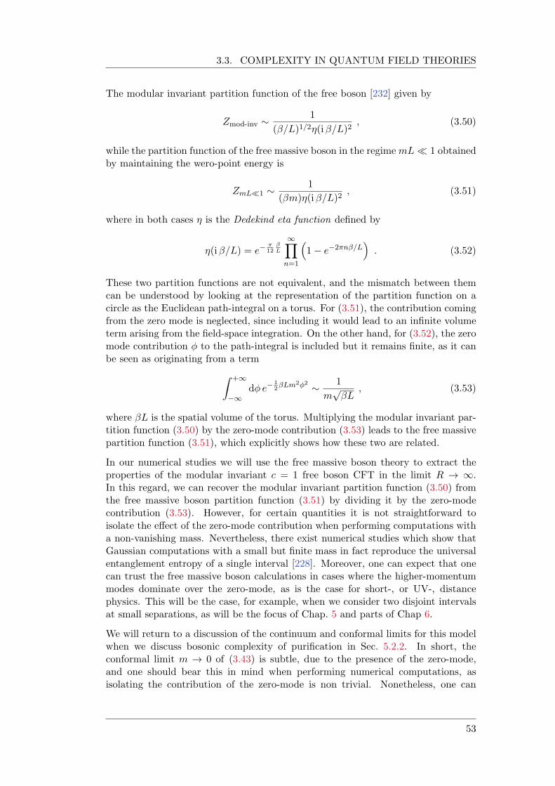
3.3. COMPLEXITY IN QUANTUM FIELD THEORIES
The modular invariant partition function of the free boson [232] given by
Zmod-inv 1
(/L)1/2(i/L)2, (3.50)
while the partition function of the free massive boson in the regimemL 1 obtainedby maintaining the wero-point energy is
ZmL1 1
(m)(i/L)2, (3.51)
where in both cases is the Dedekind eta function defined by
(i/L) = eπ12
β
L
1Y
n=1
1 e2πnβ/L
. (3.52)
These two partition functions are not equivalent, and the mismatch between themcan be understood by looking at the representation of the partition function on acircle as the Euclidean path-integral on a torus. For (3.51), the contribution comingfrom the zero mode is neglected, since including it would lead to an infinite volumeterm arising from the field-space integration. On the other hand, for (3.52), the zeromode contribution to the path-integral is included but it remains finite, as it canbe seen as originating from a term
Z +1
1d e
12βLm2φ2 1
mpL
, (3.53)
where L is the spatial volume of the torus. Multiplying the modular invariant par-tition function (3.50) by the zero-mode contribution (3.53) leads to the free massivepartition function (3.51), which explicitly shows how these two are related.
In our numerical studies we will use the free massive boson theory to extract theproperties of the modular invariant c = 1 free boson CFT in the limit R ! 1.In this regard, we can recover the modular invariant partition function (3.50) fromthe free massive boson partition function (3.51) by dividing it by the zero-modecontribution (3.53). However, for certain quantities it is not straightforward toisolate the effect of the zero-mode contribution when performing computations witha non-vanishing mass. Nevertheless, there exist numerical studies which show thatGaussian computations with a small but finite mass in fact reproduce the universalentanglement entropy of a single interval [228]. Moreover, one can expect that onecan trust the free massive boson calculations in cases where the higher-momentummodes dominate over the zero-mode, as is the case for short-, or UV-, distancephysics. This will be the case, for example, when we consider two disjoint intervalsat small separations, as will be the focus of Chap. 5 and parts of Chap 6.
We will return to a discussion of the continuum and conformal limits for this modelwhen we discuss bosonic complexity of purification in Sec. 5.2.2. In short, theconformal limit m ! 0 of (3.43) is subtle, due to the presence of the zero-mode,and one should bear this in mind when performing numerical computations, asisolating the contribution of the zero-mode is non trivial. Nonetheless, one can
53
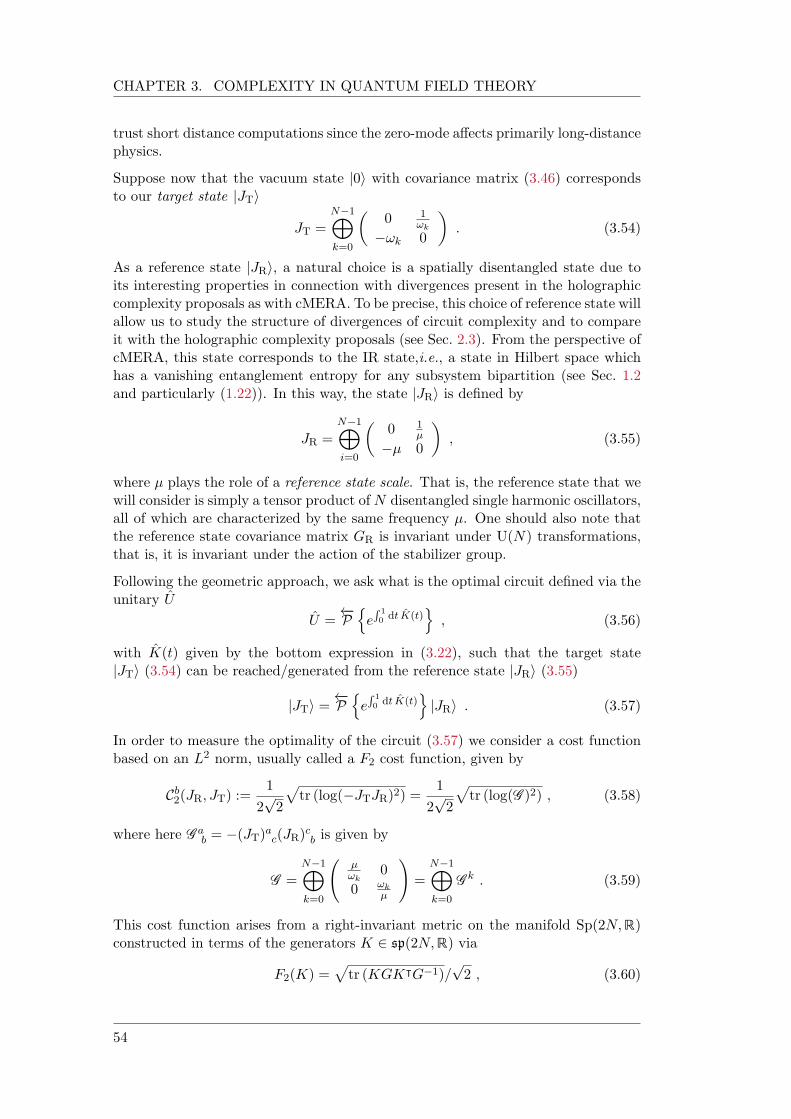
CHAPTER 3. COMPLEXITY IN QUANTUM FIELD THEORY
trust short distance computations since the zero-mode affects primarily long-distancephysics.
Suppose now that the vacuum state |0i with covariance matrix (3.46) correspondsto our target state |JTi
JT =N1M
k=0
0 1
ωk
!k 0
. (3.54)
As a reference state |JRi, a natural choice is a spatially disentangled state due toits interesting properties in connection with divergences present in the holographiccomplexity proposals as with cMERA. To be precise, this choice of reference state willallow us to study the structure of divergences of circuit complexity and to compareit with the holographic complexity proposals (see Sec. 2.3). From the perspective ofcMERA, this state corresponds to the IR state,i.e., a state in Hilbert space whichhas a vanishing entanglement entropy for any subsystem bipartition (see Sec. 1.2and particularly (1.22)). In this way, the state |JRi is defined by
JR =N1M
i=0
0 1
µ
µ 0
, (3.55)
where µ plays the role of a reference state scale. That is, the reference state that wewill consider is simply a tensor product ofN disentangled single harmonic oscillators,all of which are characterized by the same frequency µ. One should also note thatthe reference state covariance matrix GR is invariant under U(N) transformations,that is, it is invariant under the action of the stabilizer group.
Following the geometric approach, we ask what is the optimal circuit defined via theunitary U
U = PneR 10 dt K(t)
o, (3.56)
with K(t) given by the bottom expression in (3.22), such that the target state|JTi (3.54) can be reached/generated from the reference state |JRi (3.55)
|JTi = PneR 10 dt K(t)
o|JRi . (3.57)
In order to measure the optimality of the circuit (3.57) we consider a cost functionbased on an L2 norm, usually called a F2 cost function, given by
Cb2(JR, JT) :=
1
2p2
ptr (log(JTJR)2) =
1
2p2
ptr (log(G )2) , (3.58)
where here G ab = (JT)ac(JR)cb is given by
G =N1M
k=0
µωk
0
0 ωk
µ
!=
N1M
k=0
Gk . (3.59)
This cost function arises from a right-invariant metric on the manifold Sp(2N,R)constructed in terms of the generators K 2 sp(2N,R) via
F2(K) =ptr (KGK|G1)/
p2 , (3.60)
54
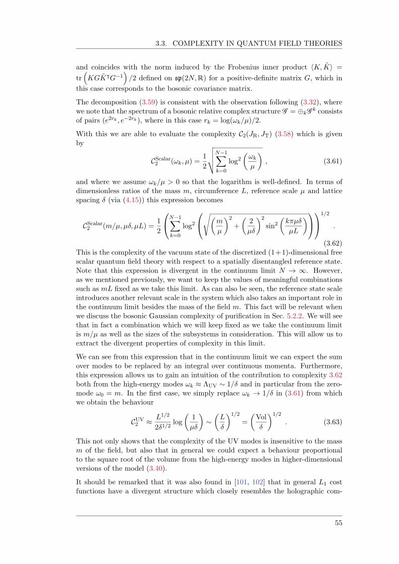
3.3. COMPLEXITY IN QUANTUM FIELD THEORIES
and coincides with the norm induced by the Frobenius inner product hK, Ki =
trKGK|G1
/2 defined on sp(2N,R) for a positive-definite matrix G, which in
this case corresponds to the bosonic covariance matrix.
The decomposition (3.59) is consistent with the observation following (3.32), wherewe note that the spectrum of a bosonic relative complex structure G = kG
k consistsof pairs (e2rk , e2rk), where in this case rk = log(!k/µ)/2.
With this we are able to evaluate the complexity C2(JR, JT) (3.58) which is givenby
CScalar2 (!k, µ) =
1
2
vuutN1X
k=0
log2!k
µ
, (3.61)
and where we assume !k/µ > 0 so that the logarithm is well-defined. In terms ofdimensionless ratios of the mass m, circumference L, reference scale µ and latticespacing (via (4.15)) this expression becomes
CScalar2 (m/µ, µ, µL) =
1
2
0@
N1X
k=0
log2
0@s
m
µ
2
+
2
µ
2
sin2kµ
µL
1A1A
1/2
.
(3.62)This is the complexity of the vacuum state of the discretized (1+1)-dimensional freescalar quantum field theory with respect to a spatially disentangled reference state.Note that this expression is divergent in the continuum limit N ! 1. However,as we mentioned previously, we want to keep the values of meaningful combinationssuch as mL fixed as we take this limit. As can also be seen, the reference state scaleintroduces another relevant scale in the system which also takes an important role inthe continuum limit besides the mass of the field m. This fact will be relevant whenwe discuss the bosonic Gaussian complexity of purification in Sec. 5.2.2. We will seethat in fact a combination which we will keep fixed as we take the continuum limitis m/µ as well as the sizes of the subsystems in consideration. This will allow us toextract the divergent properties of complexity in this limit.
We can see from this expression that in the continuum limit we can expect the sumover modes to be replaced by an integral over continuous momenta. Furthermore,this expression allows us to gain an intuition of the contribution to complexity 3.62both from the high-energy modes !k ΛUV 1/ and in particular from the zero-mode !0 = m. In the first case, we simply replace !k ! 1/ in (3.61) from whichwe obtain the behaviour
CUV2 L1/2
21/2log
1
µ
L
1/2
=
Vol
1/2
. (3.63)
This not only shows that the complexity of the UV modes is insensitive to the massm of the field, but also that in general we could expect a behaviour proportionalto the square root of the volume from the high-energy modes in higher-dimensionalversions of the model (3.40).
It should be remarked that it was also found in [101, 102] that in general L1 costfunctions have a divergent structure which closely resembles the holographic com-
55
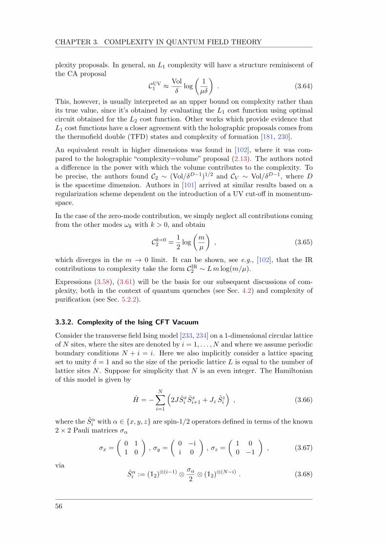
CHAPTER 3. COMPLEXITY IN QUANTUM FIELD THEORY
plexity proposals. In general, an L1 complexity will have a structure reminiscent ofthe CA proposal
CUV1 Vol
log
1
µ
. (3.64)
This, however, is usually interpreted as an upper bound on complexity rather thanits true value, since it’s obtained by evaluating the L1 cost function using optimalcircuit obtained for the L2 cost function. Other works which provide evidence thatL1 cost functions have a closer agreement with the holographic proposals comes fromthe thermofield double (TFD) states and complexity of formation [181, 230].
An equivalent result in higher dimensions was found in [102], where it was com-pared to the holographic “complexity=volume” proposal (2.13). The authors noteda difference in the power with which the volume contributes to the complexity. Tobe precise, the authors found C2 (Vol/D1)1/2 and CV Vol/D1, where Dis the spacetime dimension. Authors in [101] arrived at similar results based on aregularization scheme dependent on the introduction of a UV cut-off in momentum-space.
In the case of the zero-mode contribution, we simply neglect all contributions comingfrom the other modes !k with k > 0, and obtain
Ck=02 =
1
2log
m
µ
, (3.65)
which diverges in the m ! 0 limit. It can be shown, see e.g., [102], that the IRcontributions to complexity take the form CIR
2 Lm log(m/µ).
Expressions (3.58), (3.61) will be the basis for our subsequent discussions of com-plexity, both in the context of quantum quenches (see Sec. 4.2) and complexity ofpurification (see Sec. 5.2.2).
3.3.2. Complexity of the Ising CFT Vacuum
Consider the transverse field Ising model [233, 234] on a 1-dimensional circular latticeof N sites, where the sites are denoted by i = 1, . . . , N and where we assume periodicboundary conditions N + i = i. Here we also implicitly consider a lattice spacingset to unity = 1 and so the size of the periodic lattice L is equal to the number oflattice sites N . Suppose for simplicity that N is an even integer. The Hamiltonianof this model is given by
H = NX
i=1
2JSx
i Sxi+1 + Jz S
zi
, (3.66)
where the Sαi with ↵ 2 x, y, z are spin-1/2 operators defined in terms of the known
2 2 Pauli matrices α
x =
0 11 0
, y =
0 ii 0
, z =
1 00 1
, (3.67)
viaSαi := (12)
(i1) α
2 (12)
(Ni) . (3.68)
56
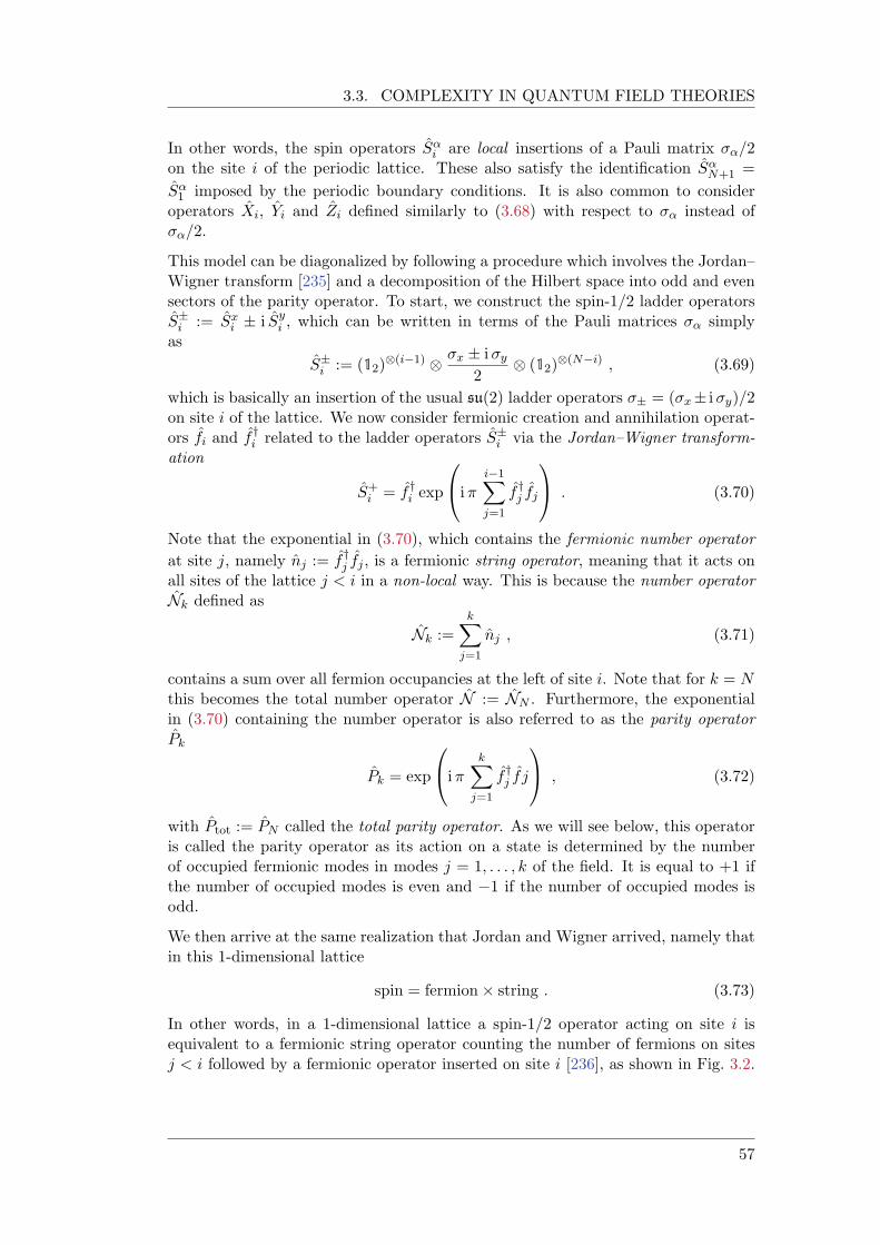
3.3. COMPLEXITY IN QUANTUM FIELD THEORIES
In other words, the spin operators Sαi are local insertions of a Pauli matrix α/2
on the site i of the periodic lattice. These also satisfy the identification SαN+1 =
Sα1 imposed by the periodic boundary conditions. It is also common to consider
operators Xi, Yi and Zi defined similarly to (3.68) with respect to α instead ofα/2.
This model can be diagonalized by following a procedure which involves the Jordan–Wigner transform [235] and a decomposition of the Hilbert space into odd and evensectors of the parity operator. To start, we construct the spin-1/2 ladder operatorsS±i := Sx
i ± i Syi , which can be written in terms of the Pauli matrices α simply
as
S±i := (12)
(i1) x ± iy2
(12)(Ni) , (3.69)
which is basically an insertion of the usual su(2) ladder operators ± = (x± iy)/2on site i of the lattice. We now consider fermionic creation and annihilation operat-ors fi and f †
i related to the ladder operators S±i via the Jordan–Wigner transform-
ation
S+i = f †
i exp
0@i
i1X
j=1
f †j fj
1A . (3.70)
Note that the exponential in (3.70), which contains the fermionic number operator
at site j, namely nj := f †j fj , is a fermionic string operator, meaning that it acts on
all sites of the lattice j < i in a non-local way. This is because the number operatorNk defined as
Nk :=
kX
j=1
nj , (3.71)
contains a sum over all fermion occupancies at the left of site i. Note that for k = Nthis becomes the total number operator N := NN . Furthermore, the exponentialin (3.70) containing the number operator is also referred to as the parity operatorPk
Pk = exp
0@i
kX
j=1
f †j f j
1A , (3.72)
with Ptot := PN called the total parity operator. As we will see below, this operatoris called the parity operator as its action on a state is determined by the numberof occupied fermionic modes in modes j = 1, . . . , k of the field. It is equal to +1 ifthe number of occupied modes is even and 1 if the number of occupied modes isodd.
We then arrive at the same realization that Jordan and Wigner arrived, namely thatin this 1-dimensional lattice
spin = fermion string . (3.73)
In other words, in a 1-dimensional lattice a spin-1/2 operator acting on site i isequivalent to a fermionic string operator counting the number of fermions on sitesj < i followed by a fermionic operator inserted on site i [236], as shown in Fig. 3.2.
57
CHAPTER 3. COMPLEXITY IN QUANTUM FIELD THEORY
Figure 3.2.: Representation of the Jordan–Wigner transformation on a lattice. the
ladder spin operator S+4 is written as the product of the fermionic cre-
ation operator f †4 and the string (parity) operator eiπ(n1+n2+n3).
This observation (3.73) has profound implications on the notion of locality, par-ticularly when splitting the lattice into two spatial subregions and tracing out thedegrees of freedom of one of them. A partial trace which is local on the spin picture isnon-local in the fermionic picture. This non-locality has unavoidable consequenceswhen computing the entanglement entropy of a spatial subregion, and therefore alsoquantities obtained thereof, such as mutual information. One should mention theinteresting series of papers [237–240] investigating dualities in spin systems and thenotion of locality from the perspective of the algebraic approach to quantum fieldtheory, based on operator algebras. We will return to this discussion in 6 when westudy entanglement of purification for adjacent and disjoint subregions. This canalso be seen more clearly be considering the inverse transformations to (3.70), whichfollowing our conventions (3.68) are given by
fi =
0@
i1Y
j=1
Zj
1A (Xi i Yi)
2, (3.74a)
f †i =
0@
i1Y
j=1
Zj
1A (Xi + i Yi)
2. (3.74b)
which shows that the transformation between spins and fermions inevitably requiresan insertion of Zi, acting as a string of operators. Let us now return to the diagon-alization of the Hamiltonian (3.66).
We can also introduce 2N Majorana modes by
2k1 := (k1)z x 1
(Nk) =
0@
k1Y
j=1
Zj
1A Xk , (3.75a)
2k := (k1)z y 1
(Nk) =
0@
k1Y
j=1
Zj
1A Yk . (3.75b)
That is, on every site i = k/2 of the lattice, we have two Majorana modes: 2k1, 2k.These are related to the fermionic operators via fk = (2k1 i 2k)/2. In terms
58
3.3. COMPLEXITY IN QUANTUM FIELD THEORIES
of Majorana modes, the total parity operator PN can be written asQN
k=1 Zk =QNk=1(i 2k12k).
We can now write the Hamiltonian (3.66) in terms of fermionic creation and anni-hilation operators. By using (3.69) we arrive at the Hamiltonian
H =NX
i=1
J
2
hf †i (fi+1 + f †
i+1) + h.c.i+ Jz f
†i fi
+J
2
hf †N (f1 + f †
1) + h.c.i(PN + 1) +
N Jz2
,
(3.76)
where the last term, namely N Jz/2 corresponds to a boundary term.
The total parity operator PN in (3.76) makes the Hamiltonian not exactly quadratic
in f †i and fi. Moreover, the presence of the term containing it makes the Hamiltonian
distinguish between sectors of even and odd eigenvalues of the total number operatorN . As a consequence, the Hilbert space of the theory can be decomposed as a directsum
H = H+ H , (3.77)
where H+ and H are eigenspaces of the total parity operator PN associated witheigenvalues ±1. This means that the fermionic Hamiltonian (3.76) can be writtenas a sum of two Hamiltonians H±
H = H+P+ + HP+ , (3.78)
with P± = (1± PN )/2 the orthogonal projectors on each of the eigenspaces
H± = Spann|n1, . . . , nN i 2 H | PN |n1, . . . , nN i = ± |n1, . . . , nN i
o, (3.79)
where ni |n1, . . . , nN i = ni |n1, . . . , nN i. The even sector H+ is usually referred toas the Neveu-Schwarz (NS) sector, while the odd sector H is referred to as theRamond (R) sector.
We can also write the Hamiltonian (3.76) in terms of Majorana modes ak = 2k1,2k as
H =i
2
12N PN + J
N1X
k=1
2k2k+1 + Jz
NX
k=1
2k12k
!. (3.80)
We are interested in the ground state |0i of the critical model J = Jz = 1 whoseHamiltonian is
H =i
2
12N PN +
2N1X
k=1
kk+1
!. (3.81)
which in terms of canonical coordinates ai = qi, pi with qi = 2i1 and pi = 2ican be written as
H =i
2
NX
i=1
(piqi+1 qipi) pN q1(PN + 1)
!. (3.82)
In the limit N !1 this leads to a lattice model of the c = 1/2 Ising CFT.
59
CHAPTER 3. COMPLEXITY IN QUANTUM FIELD THEORY
We will now focus on the even-parity sector of the theory (consistent with of choiceof even N), as it corresponds to the true ground state.2 The ground state |0i is aGaussian state, and is hence characterized by its covariance matrix
Ωabij = h | (ai bj bj ai ) | i
=1
N
X
κ
0 cos
(12 + i j)
cos(12 + j i)
0
,
(3.83)
where = πN (2k + 1) with k 2 N
2 , . . . ,N2 1 for even N . In other words,
belongs to
K+ =
N+
2k
N
k 2 Z , N
2 k N
2 1
. (3.84)
Much like in the bosonic case, in (3.83) a and b label the entries of Ωij for sites iand j of the lattice. Because of this we can write the full covariance matrix as
Ωab =
1
N
X
κ2K+
0 cos
(1+2N
2 )
cos(12N
2 )
0
, (3.85)
It is important to mention, however, that when we study fermionic complexity andentanglement of purification in Sec. 5.2.1, Sec. 6.2 and Sec. 6.3, the covariance mat-rix (3.83) as well as its infinite size limit, i.e., in the continuum limit, N !1 givenby
Ωjk =
(0 k = j(1)kj1π(kj) k 6= j
, (3.86)
will be relevant, as they will allow us to study subsystems corresponding to spatialsubregions in an efficient manner. At this point we will also return to the discussionof locality and partial traces when computing bipartite entanglement of adjacentand disjoint regions.
From (3.85) we can see that the covariance matrix can be decomposed in 2 2blocks
Ω =
N1M
k=0
0 cos (2rk)
cos (2rk) 0
=
N1M
k=0
Ωk , (3.87)
where here rk := (1 + 2k +N)/4N . It is important to note that in contrast withthe discussion in Sec. 3.2.3 where we focused on two-fermionic state systems, in thiscase we only have one fermionic state, namely |J+i at each site of the lattice. If weincluded the other state |Ji then we would have a decomposition into 4 4 blocksper site in terms of Majorana modes.
We now want to study the complexity of the ground state with respect to a Gaussianreference state. We will also consider the ground state (3.87) as our target sate,characterized by its complex structure via
JT =
N1M
k=0
0 cos (2rk)
cos (2rk) 0
, (3.88)
2For a detailed discussion see [241] and [240].
60
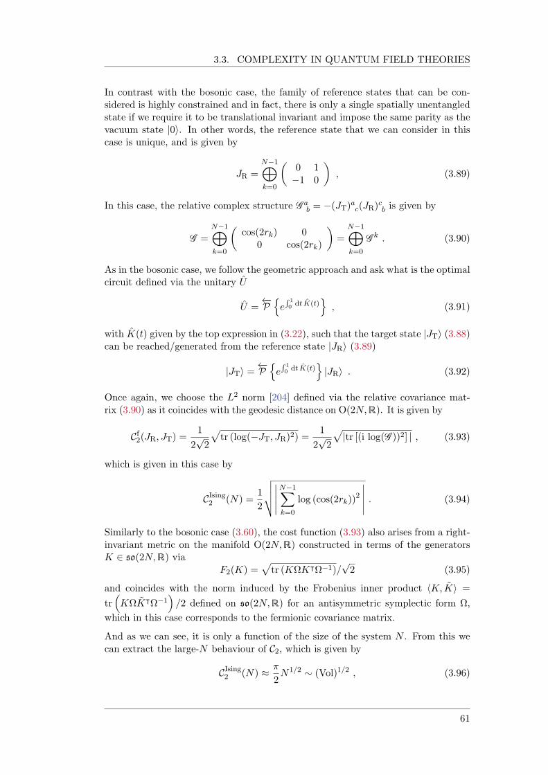
3.3. COMPLEXITY IN QUANTUM FIELD THEORIES
In contrast with the bosonic case, the family of reference states that can be con-sidered is highly constrained and in fact, there is only a single spatially unentangledstate if we require it to be translational invariant and impose the same parity as thevacuum state |0i. In other words, the reference state that we can consider in thiscase is unique, and is given by
JR =N1M
k=0
0 11 0
, (3.89)
In this case, the relative complex structure G ab = (JT)ac(JR)cb is given by
G =N1M
k=0
cos(2rk) 0
0 cos(2rk)
=
N1M
k=0
Gk . (3.90)
As in the bosonic case, we follow the geometric approach and ask what is the optimalcircuit defined via the unitary U
U = PneR 10 dt K(t)
o, (3.91)
with K(t) given by the top expression in (3.22), such that the target state |JTi (3.88)can be reached/generated from the reference state |JRi (3.89)
|JTi = PneR 10 dt K(t)
o|JRi . (3.92)
Once again, we choose the L2 norm [204] defined via the relative covariance mat-rix (3.90) as it coincides with the geodesic distance on O(2N,R). It is given by
Cf2(JR, JT) =
1
2p2
ptr (log(JT, JR)2) =
1
2p2
p|tr [(i log(G ))2] | , (3.93)
which is given in this case by
CIsing2 (N) =
1
2
vuut
N1X
k=0
log (cos(2rk))2
. (3.94)
Similarly to the bosonic case (3.60), the cost function (3.93) also arises from a right-invariant metric on the manifold O(2N,R) constructed in terms of the generatorsK 2 so(2N,R) via
F2(K) =ptr (KΩK|Ω1)/
p2 (3.95)
and coincides with the norm induced by the Frobenius inner product hK, Ki =
trKΩK|
Ω1/2 defined on so(2N,R) for an antisymmetric symplectic form Ω,
which in this case corresponds to the fermionic covariance matrix.
And as we can see, it is only a function of the size of the system N . From this wecan extract the large-N behaviour of C2, which is given by
CIsing2 (N)
2N1/2 (Vol)1/2 , (3.96)
61
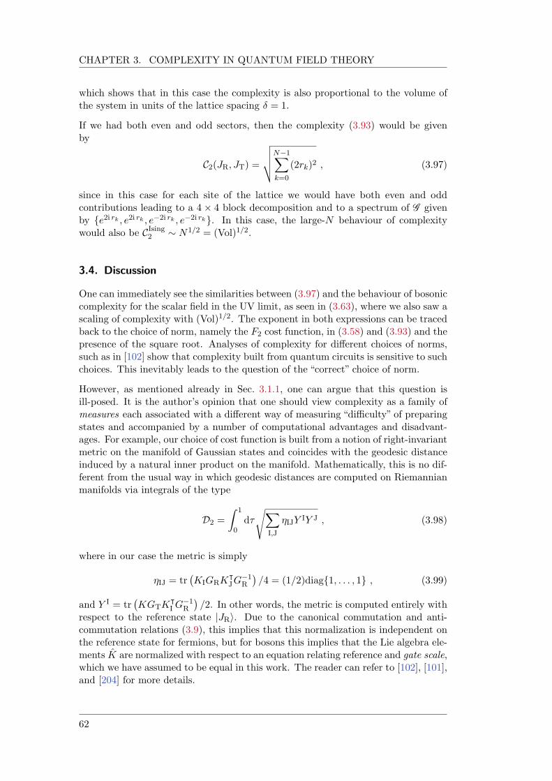
CHAPTER 3. COMPLEXITY IN QUANTUM FIELD THEORY
which shows that in this case the complexity is also proportional to the volume ofthe system in units of the lattice spacing = 1.
If we had both even and odd sectors, then the complexity (3.93) would be givenby
C2(JR, JT) =
vuutN1X
k=0
(2rk)2 , (3.97)
since in this case for each site of the lattice we would have both even and oddcontributions leading to a 4 4 block decomposition and to a spectrum of G givenby e2i rk , e2i rk , e2i rk , e2i rk. In this case, the large-N behaviour of complexitywould also be CIsing
2 N1/2 = (Vol)1/2.
3.4. Discussion
One can immediately see the similarities between (3.97) and the behaviour of bosoniccomplexity for the scalar field in the UV limit, as seen in (3.63), where we also saw ascaling of complexity with (Vol)1/2. The exponent in both expressions can be tracedback to the choice of norm, namely the F2 cost function, in (3.58) and (3.93) and thepresence of the square root. Analyses of complexity for different choices of norms,such as in [102] show that complexity built from quantum circuits is sensitive to suchchoices. This inevitably leads to the question of the “correct” choice of norm.
However, as mentioned already in Sec. 3.1.1, one can argue that this question isill-posed. It is the author’s opinion that one should view complexity as a family ofmeasures each associated with a different way of measuring “difficulty” of preparingstates and accompanied by a number of computational advantages and disadvant-ages. For example, our choice of cost function is built from a notion of right-invariantmetric on the manifold of Gaussian states and coincides with the geodesic distanceinduced by a natural inner product on the manifold. Mathematically, this is no dif-ferent from the usual way in which geodesic distances are computed on Riemannianmanifolds via integrals of the type
D2 =
Z 1
0d
sX
I,J
IJY IY J , (3.98)
where in our case the metric is simply
IJ = trKIGRK
|JG
1R
/4 = (1/2)diag1, . . . , 1 , (3.99)
and Y I = trKGTK
|I G
1R
/2. In other words, the metric is computed entirely with
respect to the reference state |JRi. Due to the canonical commutation and anti-commutation relations (3.9), this implies that this normalization is independent onthe reference state for fermions, but for bosons this implies that the Lie algebra ele-ments K are normalized with respect to an equation relating reference and gate scale,which we have assumed to be equal in this work. The reader can refer to [102], [101],and [204] for more details.
62
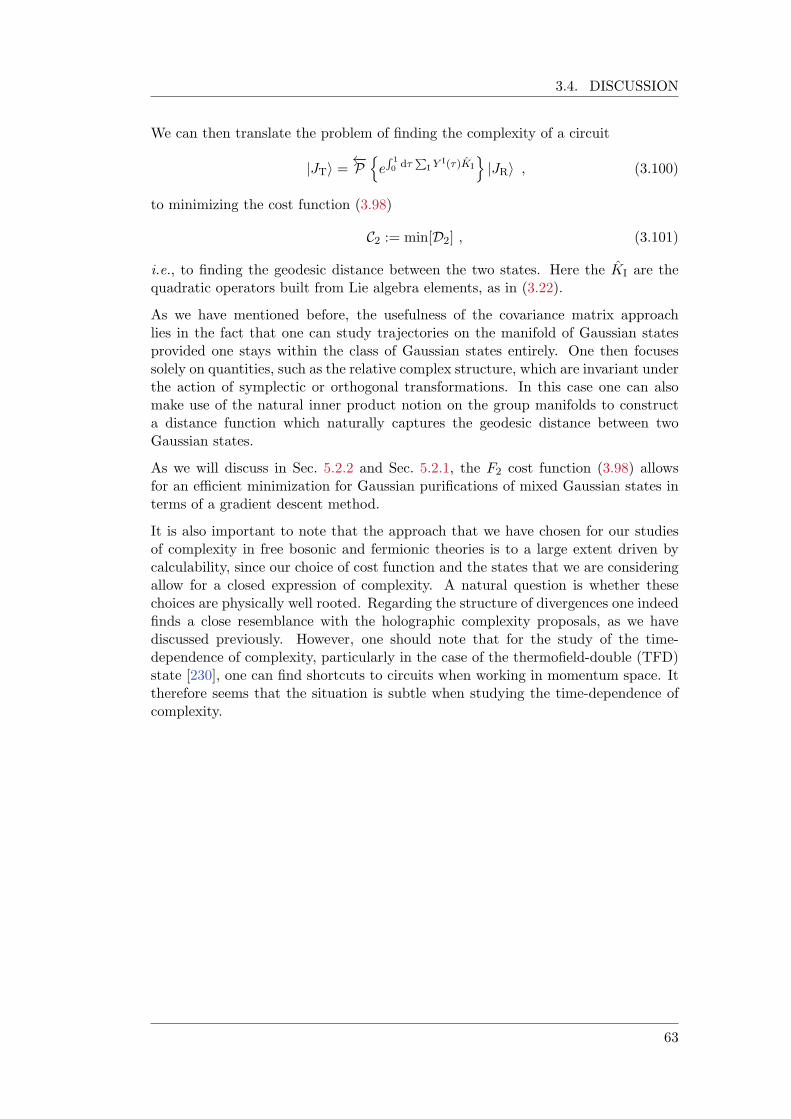
3.4. DISCUSSION
We can then translate the problem of finding the complexity of a circuit
|JTi = PneR 10 dτ
PI Y
I(τ)KI
o|JRi , (3.100)
to minimizing the cost function (3.98)
C2 := min[D2] , (3.101)
i.e., to finding the geodesic distance between the two states. Here the KI are thequadratic operators built from Lie algebra elements, as in (3.22).
As we have mentioned before, the usefulness of the covariance matrix approachlies in the fact that one can study trajectories on the manifold of Gaussian statesprovided one stays within the class of Gaussian states entirely. One then focusessolely on quantities, such as the relative complex structure, which are invariant underthe action of symplectic or orthogonal transformations. In this case one can alsomake use of the natural inner product notion on the group manifolds to constructa distance function which naturally captures the geodesic distance between twoGaussian states.
As we will discuss in Sec. 5.2.2 and Sec. 5.2.1, the F2 cost function (3.98) allowsfor an efficient minimization for Gaussian purifications of mixed Gaussian states interms of a gradient descent method.
It is also important to note that the approach that we have chosen for our studiesof complexity in free bosonic and fermionic theories is to a large extent driven bycalculability, since our choice of cost function and the states that we are consideringallow for a closed expression of complexity. A natural question is whether thesechoices are physically well rooted. Regarding the structure of divergences one indeedfinds a close resemblance with the holographic complexity proposals, as we havediscussed previously. However, one should note that for the study of the time-dependence of complexity, particularly in the case of the thermofield-double (TFD)state [230], one can find shortcuts to circuits when working in momentum space. Ittherefore seems that the situation is subtle when studying the time-dependence ofcomplexity.
63

CHAPTER 3. COMPLEXITY IN QUANTUM FIELD THEORY
64
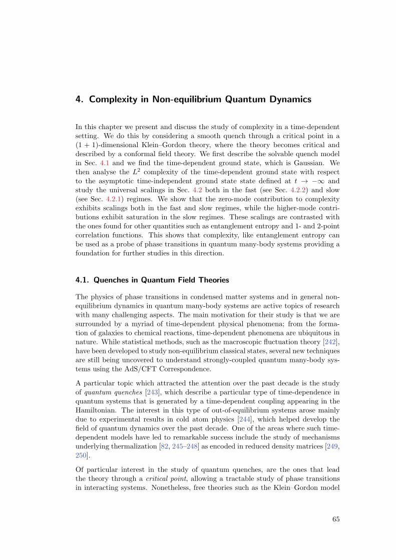
4. Complexity in Non-equilibrium Quantum Dynamics
In this chapter we present and discuss the study of complexity in a time-dependentsetting. We do this by considering a smooth quench through a critical point in a(1 + 1)-dimensional Klein–Gordon theory, where the theory becomes critical anddescribed by a conformal field theory. We first describe the solvable quench modelin Sec. 4.1 and we find the time-dependent ground state, which is Gaussian. Wethen analyse the L2 complexity of the time-dependent ground state with respectto the asymptotic time-independent ground state state defined at t ! 1 andstudy the universal scalings in Sec. 4.2 both in the fast (see Sec. 4.2.2) and slow(see Sec. 4.2.1) regimes. We show that the zero-mode contribution to complexityexhibits scalings both in the fast and slow regimes, while the higher-mode contri-butions exhibit saturation in the slow regimes. These scalings are contrasted withthe ones found for other quantities such as entanglement entropy and 1- and 2-pointcorrelation functions. This shows that complexity, like entanglement entropy canbe used as a probe of phase transitions in quantum many-body systems providing afoundation for further studies in this direction.
4.1. Quenches in Quantum Field Theories
The physics of phase transitions in condensed matter systems and in general non-equilibrium dynamics in quantum many-body systems are active topics of researchwith many challenging aspects. The main motivation for their study is that we aresurrounded by a myriad of time-dependent physical phenomena; from the forma-tion of galaxies to chemical reactions, time-dependent phenomena are ubiquitous innature. While statistical methods, such as the macroscopic fluctuation theory [242],have been developed to study non-equilibrium classical states, several new techniquesare still being uncovered to understand strongly-coupled quantum many-body sys-tems using the AdS/CFT Correspondence.
A particular topic which attracted the attention over the past decade is the studyof quantum quenches [243], which describe a particular type of time-dependence inquantum systems that is generated by a time-dependent coupling appearing in theHamiltonian. The interest in this type of out-of-equilibrium systems arose mainlydue to experimental results in cold atom physics [244], which helped develop thefield of quantum dynamics over the past decade. One of the areas where such time-dependent models have led to remarkable success include the study of mechanismsunderlying thermalization [82, 245–248] as encoded in reduced density matrices [249,250].
Of particular interest in the study of quantum quenches, are the ones that leadthe theory through a critical point, allowing a tractable study of phase transitionsin interacting systems. Nonetheless, free theories such as the Klein–Gordon model
65
CHAPTER 4. COMPLEXITY IN NON-EQUILIBRIUM QUANTUMDYNAMICS
described in Sec. 3.3.1 are also used as interesting models to study the emergenceof universal properties, such as scalings, for interesting observables. For example,if one takes the mass in (3.40) to be time-dependent such that at time t0 the massgoes to zero, then at this point the theory becomes critical, in this case becomingconformally invariant. When the mass is abruptly taken to zero, e.g., via a step-function, this leads to an instant quench corresponding to a discontinuous phasetransition. If one takes the mass to zero in a smooth way, i.e., with a smoothfunction m(t), then this type of quench is called smooth.
In this case one can also control how fast the theory approaches its critical point.This turns out to be a crucial aspect of the study of smooth quenches since de-pending how slow or how fast this critical point is reached, it will ultimately leadto different scaling behaviour for observables in the theory. In this regard, one cantypically distinguish between two different regimes. One such regime, often calledthe Kibble–Zurek (KZ) regime [251, 252], occurs when the approach to criticality isdone slowly in an attempt to adiabatically evolve the system. This regime attracteda considerable amount of attention in the last decade both in the context of theAdS/CFT correspondence and in quantum field theories [253–257].
On the other hand, one can also evolve the system in a “fast” non-adiabatic way,leading to a different scaling behaviour than the KZ regime. This regime, which hasbeen studied in the AdS/CFT Correspondence [258–262], free field theory [263–266]and lattice spin models [267, 268], also appears to lead to universal scalings presentin interacting theories which flow from a conformal field theory [269, 270]. Most ofthese studies focused on a particular class of one and two point functions, althoughmore recent works also studied the universal scaling of entanglement entropy [271–273] and complexity [274, 275, CamH03].
It is worth noting that there are several motivations for studying complexity in thecontext of quantum quenches. On one hand, it allows to study the time-dependenceof complexity in simple yet revealing models bringing its study closer to the ori-ginal motivation in the AdS/CFT correspondence where, as we saw in Sec. 2.3, thetime-dependence of the holographic complexity proposals was crucial to establish-ing a connection with a notion of complexity. On the other hand it is interestingto determine whether complexity also exhibits universal scalings like entanglemententropy, and to compare them. At the same time, since entanglement entropy iscomputed for a reduced density matrix corresponding to spatial subsystems andcomplexity for the full pure state, it is interesting to determine how the physicalinformation of the system undergoing the quench is captured distinctly by complex-ity and entanglement. In a following chapter, Ch. 5, we will explicitly consider anotion of complexity for spatial subsystems which probes to the same amount ofinformation about the system as entanglement entropy.
We will now describe a particular solvable quench protocol in Sec. 4.1.1 and thenproceed to study the universal scalings of circuit complexity of the vacuum statein both regimes in Sec. 4.2. First we will do this for a single bosonic mode,i.e.,for a harmonic oscillator and then we will consider a lattice of oscillators, such asin (3.41).
66
4.1. QUENCHES IN QUANTUM FIELD THEORIES
4.1.1. A Solvable Quench Model
We begin by considering a single harmonic oscillator described by the followingtime-dependent Hamiltonian
H(t) =1
2p2 +
1
2!2(t/t)q2 , (4.1)
where t is the quench rate or quench parameter and where !(t/t) is a time-dependent frequency profile. We introduce this quench parameter in order to have!(t/t) varying over one unit of its argument. Here = q, p are canonical (dimen-sionless) variables which satisfy [q, p] = i. Note that in principle one can also chooseto work with dimensionful variables by introducing a mass M , although this doesn’talter our analysis of complexity, as such a mass would get adjusted by appropriatelychoosing a gate scale.
In order to find the time-dependent ground state, we propose a solution of theequations of motion
d2 q(t)
dt2+ !2(t/t)q(t) = 0 , p(t) =
d q(t)
dt, (4.2)
of the formq(t) = f(t)a+ f(t)a† , (4.3a)
p(t) =d f(t)
dta+
d f(t)dt
a† , (4.3b)
where f(t) is a time-dependent complex function and where a, a† are annihilationand creation operators respectively, which satisfy [a, a†] = 1. Here f(t) denotes thecomplex conjugate of f(t). This leads to the following Wronskian constraint forf(t)
f(t)d f(t)dt
f(t)d f(t)
dt= i , (4.4)
where now f(t) is a solution of the equation of motion
d2 f(t)
dt2+ !2(t/t)f(t) = 0 , (4.5)
for all t. We choose the asymptotic boundary condition
f(t! 1)! fin(t) =1p2!in
eiωint , (4.6)
where !in := !(t! 1). Even though we do not explicitly write down the depend-ence on t, the reader should be aware that the time-dependent function f(t) is inreality a function of the ratio t/t. That is, we want our system to start with the“in” vacuum of the asymptotic (time-independent) Hamiltonian at t! 1.
We now construct the time-dependent ground state | 0i by imposing that it isannihilated by a
a | 0i = id f(t)dt
q f(t)p
| 0i = 0 . (4.7)
67
CHAPTER 4. COMPLEXITY IN NON-EQUILIBRIUM QUANTUMDYNAMICS
In position space this condition becomes the following differential equation for theground state wavefunction 0(q, t)
d f(t)dt
q + i f(t)d
dq
0(q, t) = 0 , (4.8)
which is solved by
0(q, t) =
1
2 f(t)f(t)
1/4
exp
i
1
f(t)d f(t)dt
q2
2
. (4.9)
This is the most general ground state solution to the time-dependent equations ofmotion for a generic frequency profile !(t/t). Of course, we still need to find asolution f(t) to (4.5) for a specific profile, but we have already found the generalform of the ground state wavefunction. We can immediately see that this is a Gaus-sian state, as expected. In particular, we can bring the wavefunction (4.9) to theform (3.13), where now a(t) and b(t) are time-dependent real-valued functions cor-responding to the real and imaginary parts of i(1/f(t))(d f(t)/dt). The preciseform of a(t) and b(t) in this case is not particularly revealing, although one can cer-tainly do the algebra to obtain them in terms of the real and imaginary part of f(t)and their time-derivatives. The normalizability condition a(t) > 0 is now imposedon the function f(t).
One can also see that at early times the ground state solution is simply given by
0(q, t! 1) = in0 (q) =
!in
1/4exp
!in q
2
2
, (4.10)
which is the“in”vacuum ground state obtained simply by taking (4.6) in (4.9).
What we now need is a particular quench profile !(t/t) with the properties that wediscussed at the beginning of this chapter; that is, a profile which asymptotes to aconstant both at early and late times and which takes the theory through a criticalpoint in the interval [t, t]. One such profile, which has also been used to studythe scalings of entanglement entropy [272], is:
!(t/t) = !0
1 1
cosh2
tδt
!1/2
= !0 tanh
t
t
, (4.11)
where !0 is a free parameter corresponding to the “in” asymptotic value of thefrequency !0 = !in. As we can see from Fig. 4.1, the quench parameter t controlshow fast the system approaches the critical point at t = 0 where !(0) = 0. Inparticular, one can see that for t !1
0 the approach to the critical point att = 0 is “slow”. This corresponds to the Kibble–Zurek regime, which we alreadymentioned in the introduction to this chapter. On the other hand for 0 < t < !1
0 ,the approach to the critical point is more sudden, corresponding to the “fast” quenchregime and which in the limit t! 0 corresponds to a sudden quench. We will returnto an analysis these two regimes in Sec. 4.2.1 and Sec. 4.2.2 respectively.
With this profile it is possible solve the equation (4.5) for !(t/) given by (4.11),which now takes the form
f 00() + w20 tanh
2 () f() = 0 , (4.12)
68
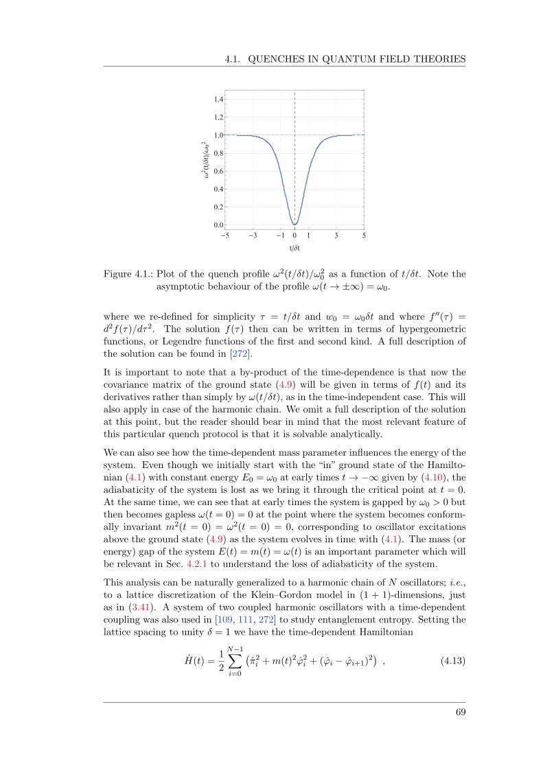
4.1. QUENCHES IN QUANTUM FIELD THEORIES
-5 -3 -1 0 1 3 5
0.0
0.2
0.4
0.6
0.8
1.0
1.2
1.4
t/ t
2(t/t)/02
Figure 4.1.: Plot of the quench profile !2(t/t)/!20 as a function of t/t. Note the
asymptotic behaviour of the profile !(t! ±1) = !0.
where we re-defined for simplicity = t/t and w0 = !0t and where f 00() =d2f()/d2. The solution f() then can be written in terms of hypergeometricfunctions, or Legendre functions of the first and second kind. A full description ofthe solution can be found in [272].
It is important to note that a by-product of the time-dependence is that now thecovariance matrix of the ground state (4.9) will be given in terms of f(t) and itsderivatives rather than simply by !(t/t), as in the time-independent case. This willalso apply in case of the harmonic chain. We omit a full description of the solutionat this point, but the reader should bear in mind that the most relevant feature ofthis particular quench protocol is that it is solvable analytically.
We can also see how the time-dependent mass parameter influences the energy of thesystem. Even though we initially start with the “in” ground state of the Hamilto-nian (4.1) with constant energy E0 = !0 at early times t! 1 given by (4.10), theadiabaticity of the system is lost as we bring it through the critical point at t = 0.At the same time, we can see that at early times the system is gapped by !0 > 0 butthen becomes gapless !(t = 0) = 0 at the point where the system becomes conform-ally invariant m2(t = 0) = !2(t = 0) = 0, corresponding to oscillator excitationsabove the ground state (4.9) as the system evolves in time with (4.1). The mass (orenergy) gap of the system E(t) = m(t) = !(t) is an important parameter which willbe relevant in Sec. 4.2.1 to understand the loss of adiabaticity of the system.
This analysis can be naturally generalized to a harmonic chain of N oscillators; i.e.,to a lattice discretization of the Klein–Gordon model in (1 + 1)-dimensions, justas in (3.41). A system of two coupled harmonic oscillators with a time-dependentcoupling was also used in [109, 111, 272] to study entanglement entropy. Setting thelattice spacing to unity = 1 we have the time-dependent Hamiltonian
H(t) =1
2
N1X
i=0
2i +m(t)2'2
i + ('i 'i+1)2, (4.13)
69
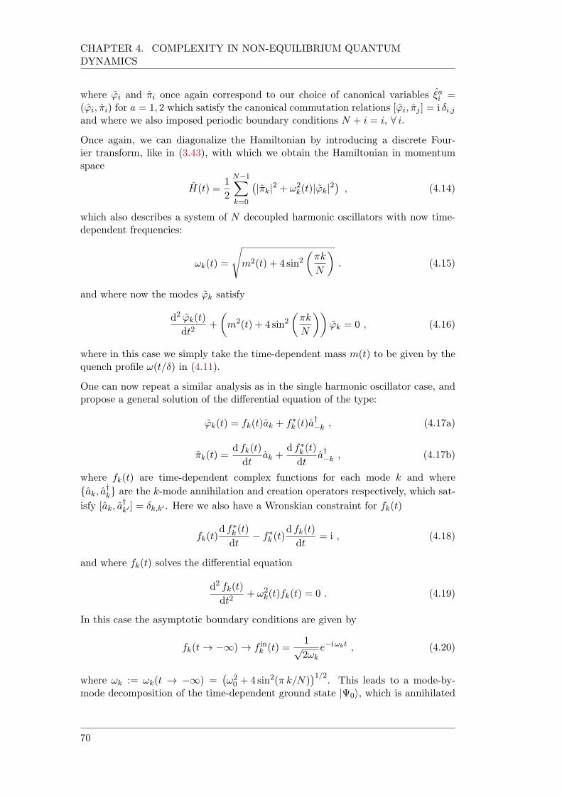
CHAPTER 4. COMPLEXITY IN NON-EQUILIBRIUM QUANTUMDYNAMICS
where 'i and i once again correspond to our choice of canonical variables ai =('i, i) for a = 1, 2 which satisfy the canonical commutation relations ['i, j ] = i i,jand where we also imposed periodic boundary conditions N + i = i, 8 i.
Once again, we can diagonalize the Hamiltonian by introducing a discrete Four-ier transform, like in (3.43), with which we obtain the Hamiltonian in momentumspace
H(t) =1
2
N1X
k=0
|k|
2 + !2k(t)|'k|
2, (4.14)
which also describes a system of N decoupled harmonic oscillators with now time-dependent frequencies:
!k(t) =
sm2(t) + 4 sin2
k
N
. (4.15)
and where now the modes 'k satisfy
d2 'k(t)
dt2+
m2(t) + 4 sin2
k
N
'k = 0 , (4.16)
where in this case we simply take the time-dependent mass m(t) to be given by thequench profile !(t/) in (4.11).
One can now repeat a similar analysis as in the single harmonic oscillator case, andpropose a general solution of the differential equation of the type:
'k(t) = fk(t)ak + fk (t)a
†k , (4.17a)
k(t) =d fk(t)
dtak +
d fk (t)
dta†k , (4.17b)
where fk(t) are time-dependent complex functions for each mode k and where
ak, a†k are the k-mode annihilation and creation operators respectively, which sat-
isfy [ak, a†k0 ] = k,k0 . Here we also have a Wronskian constraint for fk(t)
fk(t)d f
k (t)
dt f
k (t)d fk(t)
dt= i , (4.18)
and where fk(t) solves the differential equation
d2 fk(t)
dt2+ !2
k(t)fk(t) = 0 . (4.19)
In this case the asymptotic boundary conditions are given by
fk(t! 1)! f ink (t) =
1p2!k
eiωkt , (4.20)
where !k := !k(t ! 1) =!20 + 4 sin2( k/N)
1/2. This leads to a mode-by-
mode decomposition of the time-dependent ground state |Ψ0i, which is annihilated
70
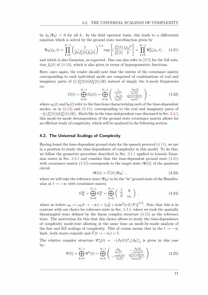
4.2. THE UNIVERSAL SCALINGS OF COMPLEXITY
by ak |Ψ0i = 0 for all k. In the field operator basis, this leads to a differentialequation which is solved by the ground state wavefunction given by
Ψ0('k, t) =N1Y
k=0
1
2fk (t)fk(t)
1/4
exp
"ifk (t)
fk (t)
|'k|2
2
#=
N1Y
k=0
Ψk0('k, t) , (4.21)
and which is also Gaussian, as expected. One can also refer to [272] for the full solu-tion fk(t) of (4.19), which is also given in terms of hypergeometric functions.
Here, once again, the reader should note that the entries of the covariance matrixcorresponding to each individual mode are comprised of combinations of real andimaginary parts of (i/f
k (t))(dfk (t)/dt) instead of simply the k-mode frequencies
!k:
G(t) =
N1M
k=0
Gk(t) =
N1M
k=0
1
ak(t)bk(t)ak(t)
bk(t)ak(t)
a2k(t)+b2
k(t)
ak(t)
!, (4.22)
where ak(t) and bk(t) refer to the functions characterizing each of the time-dependentmodes, as in (3.13) and (3.15), corresponding to the real and imaginary parts of(i/f
k (t))(dfk (t)/dt). Much like in the time-independent case discussed in Sec. 3.3.1,
this mode-by-mode decomposition of the ground state covariance matrix allows foran efficient study of complexity, which will be analysed in the following section.
4.2. The Universal Scalings of Complexity
Having found the time-dependent ground state for the quench protocol (4.11), we arein a position to study the time-dependence of complexity in this model. To do this,we follow the geometric procedure described in Sec. 3.1.1 applied to bosonic Gaus-sian states in Sec. 3.3.1 and consider that the time-dependent ground state (4.21)with covariance matrix (4.22) corresponds to the target state |Ψ(t)i of the quantumcircuit
|Ψ(t)i = U(t) |ΨRi , (4.23)
where we will take the reference state |ΨRi to be the“in”ground state of the Hamilto-nian at t! 1 with covariance matrix
GinR =
N1M
k=0
Gink =
N1M
k=0
1ωk
0
0 !k
, (4.24)
where as before !k := !k(t ! 1) =!20 + 4 sin2( k/N)
1/2. Note that this is in
contrast with our choice for reference state in Sec. 3.3.1, where we took the spatiallydisentangled state defined by the linear complex structure (3.55) as the referencestate. The motivation for this that this choice allows to study the time-dependenceof complexity mode-wise allowing at the same time an mode-by-mode analysis ofthe fast and KZ scalings of complexity. This of course means that in the t ! 1limit, both states coincide and U(t! 1) = 1.
The relative complex structure G ab(t) = (JT(t))ac(JR)cb is given in this case
by:
G (t) =N1M
k=0
Gk(t) =
N1M
k=0
ωk
ak(t) bk(t)
ωkak(t)
ωkbk(t)ak(t)
a2k(t)+b2
k(t)
ωkak(t)
!. (4.25)
71
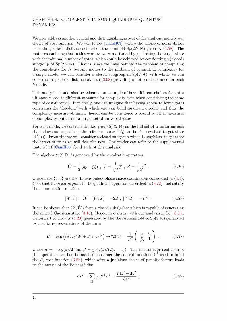
CHAPTER 4. COMPLEXITY IN NON-EQUILIBRIUM QUANTUMDYNAMICS
We now address another crucial and distinguishing aspect of the analysis, namely ourchoice of cost function. We will follow [CamH03], where the choice of norm differsfrom the geodesic distance defined on the manifold Sp(2N,R) given by (3.58). Themain reason being that in this work we were motivated by generating the target statewith the minimal number of gates, which could be achieved by considering a (closed)subgroup of Sp(2N,R). That is, since we have reduced the problem of computingthe complexity for N bosonic modes to the problem of computing complexity fora single mode, we can consider a closed subgroup in Sp(2,R) with which we canconstruct a geodesic distance akin to (3.98) providing a notion of distance for eachk-mode.
This analysis should also be taken as an example of how different choices for gatesultimately lead to different measures for complexity even when considering the sametype of cost-function. Intuitively, one can imagine that having access to fewer gatesconstrains the “freedom” with which one can build quantum circuits and thus thecomplexity measure obtained thereof can be considered a bound to other measuresof complexity built from a larger set of universal gates.
For each mode, we consider the Lie group Sp(2,R) as the full set of transformationsthat allows us to get from the reference state |Ψk
Ri to the time-evolved target state|Ψk
T(t)i. From this we will consider a closed subgroup which is sufficient to generatethe target state as we will describe now. The reader can refer to the supplementalmaterial of [CamH03] for details of this analysis.
The algebra sp(2,R) is generated by the quadratic operators
W =i
2(qp+ pq) , V =
ip2q2 , Z =
ip2p2 , (4.26)
where here q, p are the dimensionless phase space coordinates considered in (4.1).Note that these correspond to the quadratic operators described in (3.22), and satisfythe commutation relations
[W , V ] = 2V , [W , Z] = 2Z , [V , Z] = 2W . (4.27)
It can be shown that V , W form a closed subalgebra which is capable of generatingthe general Gaussian state (3.15). Hence, in contrast with our analysis in Sec. 3.3.1,we restrict to circuits (4.23) generated by the the submanifold of Sp(2,R) generatedby matrix representations of the form
U = exp↵(z, y)W + (z, y)V
! R(U) =
1pz
z 0yp2
1
!, (4.28)
where ↵ = log(z)/2 and = y log(z)/(2(z 1)). The matrix representation ofthis operator can then be used to construct the control functions Y I used to buildthe F2 cost function (3.8b), which after a judicious choice of penalty factors leadsto the metric of the Poincare disc
ds2 =X
IJ
gIJYIY J =
2dz2 + dy2
8z2, (4.29)
72
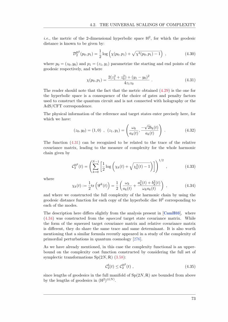
4.2. THE UNIVERSAL SCALINGS OF COMPLEXITY
i.e., the metric of the 2-dimensional hyperbolic space H2, for which the geodesic
distance is known to be given by:
DH2
2 (p0, p1) =1
2log
(p0, p1) +
p2(p0, p1) 1
, (4.30)
where p0 = (z0, y0) and p1 = (z1, y1) parametrize the starting and end points of thegeodesic respectively, and where
(p0, p1) =2(z21 + z20) + (y1 y0)
2
4z1z0. (4.31)
The reader should note that the fact that the metric obtained (4.29) is the one forthe hyperbolic space is a consequence of the choice of gates and penalty factorsused to construct the quantum circuit and is not connected with holography or theAdS/CFT correspondence.
The physical information of the reference and target states enter precisely here, forwhich we have:
(z0, y0) = (1, 0) , (z1, y1) =
!k
ak(t),p2bk(t)
ak(t)
!. (4.32)
The function (4.31) can be recognized to be related to the trace of the relativecovariance matrix, leading to the measure of complexity for the whole harmonicchain given by
CH2
2 (t) =
N1X
k=0
1
2log
k(t) +
q2k(t) 1
!1/2
, (4.33)
where
k(t) :=1
2trG
k(t)=
1
2
!k
ak(t)+
a2k(t) + b2k(t)
!kak(t)
, (4.34)
and where we constructed the full complexity of the harmonic chain by using thegeodesic distance function for each copy of the hyperbolic disc H
2 corresponding toeach of the modes.
The description here differs slightly from the analysis present in [CamH03], where(4.34) was constructed from the squeezed target state covariance matrix. Whilethe form of the squeezed target covariance matrix and relative covariance matrixis different, they do share the same trace and same determinant. It is also worthmentioning that a similar formula recently appeared in a study of the complexity ofprimordial perturbations in quantum cosmology [276].
As we have already mentioned, in this case the complexity functional is an upper-bound on the complexity cost function constructed by considering the full set ofsymplectic transformations Sp(2N,R) (3.58):
Cb2(t) CH2
2 (t) , (4.35)
since lengths of geodesics in the full manifold of Sp(2N,R) are bounded from aboveby the lengths of geodesics in (H2)(N).
73
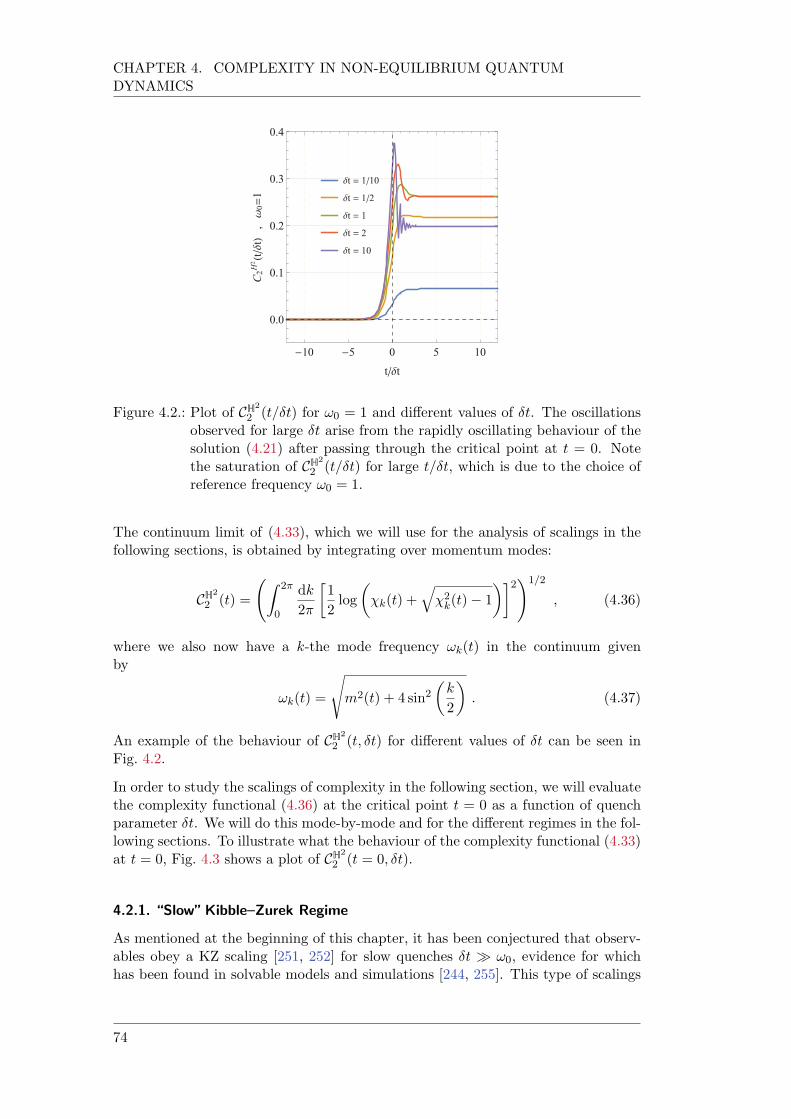
CHAPTER 4. COMPLEXITY IN NON-EQUILIBRIUM QUANTUMDYNAMICS
t = 1/10
t = 1/2
t = 1
t = 2
t = 10
-10 -5 0 5 10
0.0
0.1
0.2
0.3
0.4
t/ t
C2H2
(t/t),
0=1
Figure 4.2.: Plot of CH2
2 (t/t) for !0 = 1 and different values of t. The oscillationsobserved for large t arise from the rapidly oscillating behaviour of thesolution (4.21) after passing through the critical point at t = 0. Notethe saturation of CH2
2 (t/t) for large t/t, which is due to the choice ofreference frequency !0 = 1.
The continuum limit of (4.33), which we will use for the analysis of scalings in thefollowing sections, is obtained by integrating over momentum modes:
CH2
2 (t) =
Z 2π
0
dk
2
1
2log
k(t) +
q2k(t) 1
2!1/2
, (4.36)
where we also now have a k-the mode frequency !k(t) in the continuum givenby
!k(t) =
sm2(t) + 4 sin2
k
2
. (4.37)
An example of the behaviour of CH2
2 (t, t) for different values of t can be seen inFig. 4.2.
In order to study the scalings of complexity in the following section, we will evaluatethe complexity functional (4.36) at the critical point t = 0 as a function of quenchparameter t. We will do this mode-by-mode and for the different regimes in the fol-lowing sections. To illustrate what the behaviour of the complexity functional (4.33)at t = 0, Fig. 4.3 shows a plot of CH2
2 (t = 0, t).
4.2.1. “Slow”Kibble–Zurek Regime
As mentioned at the beginning of this chapter, it has been conjectured that observ-ables obey a KZ scaling [251, 252] for slow quenches t !0, evidence for whichhas been found in solvable models and simulations [244, 255]. This type of scalings
74
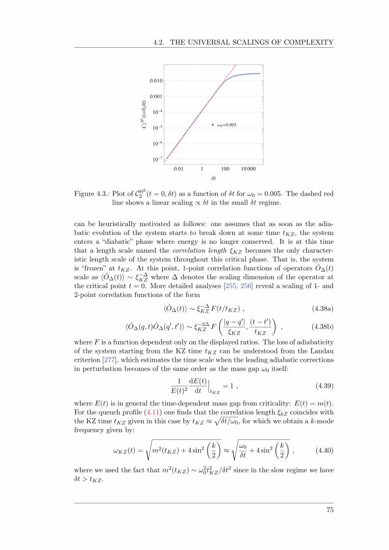
4.2. THE UNIVERSAL SCALINGS OF COMPLEXITY
0=0.005
0.01 1 100 10000
10-7
10-6
10-5
10-4
0.001
0.010
t
C2H2
(t=0,t)
Figure 4.3.: Plot of CH2
2 (t = 0, t) as a function of t for !0 = 0.005. The dashed redline shows a linear scaling / t in the small t regime.
can be heuristically motivated as follows: one assumes that as soon as the adia-batic evolution of the system starts to break down at some time tKZ , the systementers a “diabatic” phase where energy is no longer conserved. It is at this timethat a length scale named the correlation length KZ becomes the only character-istic length scale of the system throughout this critical phase. That is, the systemis “frozen” at tKZ . At this point, 1-point correlation functions of operators O∆(t)scale as hO∆(t)i ∆
KZ where ∆ denotes the scaling dimension of the operator atthe critical point t = 0. More detailed analyses [255, 256] reveal a scaling of 1- and2-point correlation functions of the form
hO∆(t)i ∆
KZ F (t/tKZ) , (4.38a)
hO∆(q, t)O∆(q0, t0)i 2∆
KZ F
|q q0|KZ
,(t t0)tKZ
, (4.38b)
where F is a function dependent only on the displayed ratios. The loss of adiabaticityof the system starting from the KZ time tKZ can be understood from the Landaucriterion [277], which estimates the time scale when the leading adiabatic correctionsin perturbation becomes of the same order as the mass gap !0 itself:
1
E(t)2dE(t)
dt
tKZ
= 1 , (4.39)
where E(t) is in general the time-dependent mass gap from criticality: E(t) = m(t).For the quench profile (4.11) one finds that the correlation length kZ coincides withthe KZ time tKZ given in this case by tKZ
pt/!0, for which we obtain a k-mode
frequency given by:
!KZ(t) =
sm2(tKZ) + 4 sin2
k
2
s!0
t+ 4 sin2
k
2
, (4.40)
where we used the fact that m2(tKZ) !20t
2KZ/t
2 since in the slow regime we havet > tKZ .
75
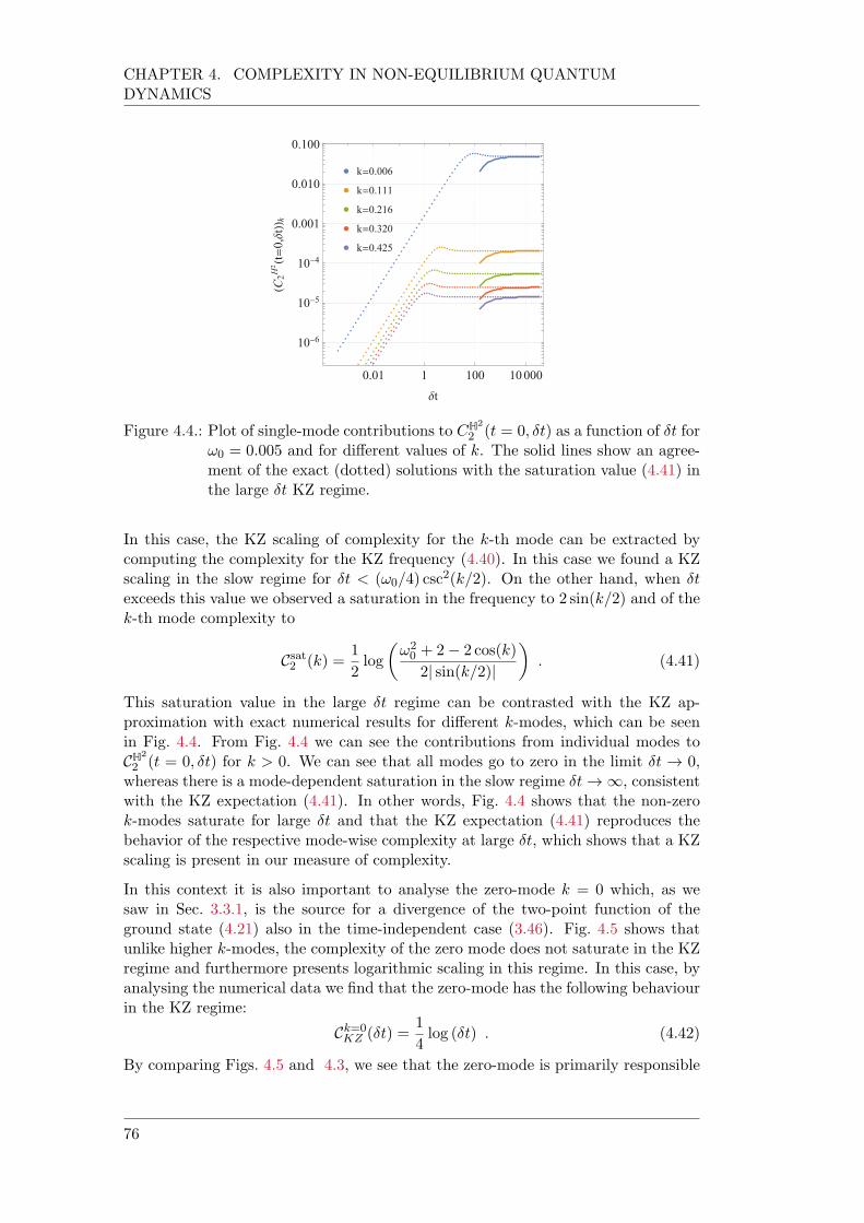
CHAPTER 4. COMPLEXITY IN NON-EQUILIBRIUM QUANTUMDYNAMICS
k=0.006
k=0.111
k=0.216
k=0.320
k=0.425
0.01 1 100 10000
10-6
10-5
10-4
0.001
0.010
0.100
t
(C2H2
(t=0,t)) k
Figure 4.4.: Plot of single-mode contributions to CH2
2 (t = 0, t) as a function of t for!0 = 0.005 and for different values of k. The solid lines show an agree-ment of the exact (dotted) solutions with the saturation value (4.41) inthe large t KZ regime.
In this case, the KZ scaling of complexity for the k-th mode can be extracted bycomputing the complexity for the KZ frequency (4.40). In this case we found a KZscaling in the slow regime for t < (!0/4) csc
2(k/2). On the other hand, when texceeds this value we observed a saturation in the frequency to 2 sin(k/2) and of thek-th mode complexity to
Csat2 (k) =
1
2log
!20 + 2 2 cos(k)
2| sin(k/2)|
. (4.41)
This saturation value in the large t regime can be contrasted with the KZ ap-proximation with exact numerical results for different k-modes, which can be seenin Fig. 4.4. From Fig. 4.4 we can see the contributions from individual modes toCH2
2 (t = 0, t) for k > 0. We can see that all modes go to zero in the limit t ! 0,whereas there is a mode-dependent saturation in the slow regime t!1, consistentwith the KZ expectation (4.41). In other words, Fig. 4.4 shows that the non-zerok-modes saturate for large t and that the KZ expectation (4.41) reproduces thebehavior of the respective mode-wise complexity at large t, which shows that a KZscaling is present in our measure of complexity.
In this context it is also important to analyse the zero-mode k = 0 which, as wesaw in Sec. 3.3.1, is the source for a divergence of the two-point function of theground state (4.21) also in the time-independent case (3.46). Fig. 4.5 shows thatunlike higher k-modes, the complexity of the zero mode does not saturate in the KZregime and furthermore presents logarithmic scaling in this regime. In this case, byanalysing the numerical data we find that the zero-mode has the following behaviourin the KZ regime:
Ck=0KZ (t) =
1
4log (t) . (4.42)
By comparing Figs. 4.5 and 4.3, we see that the zero-mode is primarily responsible
76
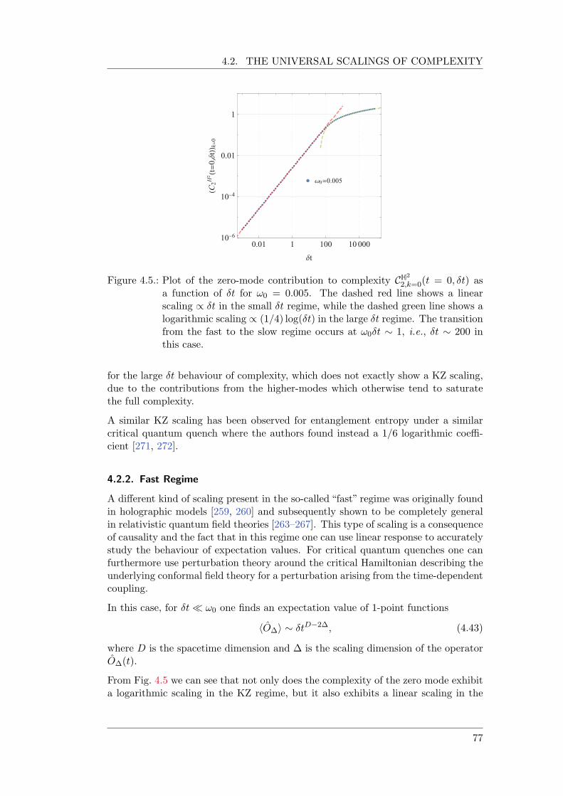
4.2. THE UNIVERSAL SCALINGS OF COMPLEXITY
0=0.005
0.01 1 100 1000010
-6
10-4
0.01
1
t
(C2H2
(t=0,t)) k
=0
Figure 4.5.: Plot of the zero-mode contribution to complexity CH2
2,k=0(t = 0, t) asa function of t for !0 = 0.005. The dashed red line shows a linearscaling / t in the small t regime, while the dashed green line shows alogarithmic scaling / (1/4) log(t) in the large t regime. The transitionfrom the fast to the slow regime occurs at !0t 1, i.e., t 200 inthis case.
for the large t behaviour of complexity, which does not exactly show a KZ scaling,due to the contributions from the higher-modes which otherwise tend to saturatethe full complexity.
A similar KZ scaling has been observed for entanglement entropy under a similarcritical quantum quench where the authors found instead a 1/6 logarithmic coeffi-cient [271, 272].
4.2.2. Fast Regime
A different kind of scaling present in the so-called “fast” regime was originally foundin holographic models [259, 260] and subsequently shown to be completely generalin relativistic quantum field theories [263–267]. This type of scaling is a consequenceof causality and the fact that in this regime one can use linear response to accuratelystudy the behaviour of expectation values. For critical quantum quenches one canfurthermore use perturbation theory around the critical Hamiltonian describing theunderlying conformal field theory for a perturbation arising from the time-dependentcoupling.
In this case, for t !0 one finds an expectation value of 1-point functions
hO∆i tD2∆, (4.43)
where D is the spacetime dimension and ∆ is the scaling dimension of the operatorO∆(t).
From Fig. 4.5 we can see that not only does the complexity of the zero mode exhibita logarithmic scaling in the KZ regime, but it also exhibits a linear scaling in the
77
CHAPTER 4. COMPLEXITY IN NON-EQUILIBRIUM QUANTUMDYNAMICS
fast regime
Ck=0fast (t) / t . (4.44)
A transition between these two regimes occurs around t!0 1.
Furthermore, in the fast regime t < !0, the full state complexity also grows linearlywith t, as can be seen from Fig. 4.3. While these fast scalings are also present forhigher modes as well, as in Fig. 4.4, the reader can see that they are confined toincreasingly narrow regions of t for larger values of k.
4.3. Discussion
One natural question to ask at this point is whether the observation of scalingsin complexity depends on the choice of norm, namely of our cost function (4.36).Fig. 4.4 shows that as we approach the UV modes, both the exact solution as wellas the KZ approximation for non-zero modes (4.41) saturate to smaller values ofcomplexity at lower values of t. However, as we already mentioned, it is the zeromode 4.5 which dominates the large t limit. This means that the full complexity,when written in terms of the Fourier (momentum) modes, approximately inheritsthe scaling behaviour of the zero mode. This in turn implies that for complexitymeasures arising from Fp cost functions with p > 2, we can generically expect thatthe full state complexity constructed from Fourier modes will be dominated by thezero mode and will also approximately inherit its logarithmic behaviour in the KZregime.
The exception to this analysis, however, is the F1 cost function (3.8a) which givesrise to an L1 norm. In this case it is not entirely clear what universal scalings canbe extracted from the full state complexity, since the saturation values for higherk-modes would not be as suppressed as in the other cases. The reason is that theexponent with which the different contributions are summed-over is 1. In this caseit is hence not clear how much the scalings of zero-mode contribution to complexitywould dominate over the higher-mode contributions.
The reader could also wonder what would happen if we considered the spatially disen-tangled reference state (3.55) as the reference state, instead of the time-independentground state. In this case, numerical studies show that only the zero-mode exhibitsequivalent scalings in both regimes, as expected, while higher k-modes do not. Thedifference between this choice and our initial choice of reference state case, is thatthe non-zero k mode saturations occur at larger values of t. Thus, in the previouscase when the small contributions from higher k-modes are squared and became sub-dominant in the k-mode sum, in this case they remain relevant. This is also the samemechanism why the F2 cost function “gets rid” of the non-zero k mode saturationsmore efficiently than the F1 cost function. When the individual mode contributionsto complexity are risen to higher powers, the non-zero saturations (which are !0)essentially become subdominant.
Similar studies were carried out in the context of the relativistic fermionic Isingtheory in [275]. In this case, a linear behaviour of complexity was also observed inthe instantaneous quench regime !0t 1, as well as a saturation of the higher
78
4.3. DISCUSSION
modes in the slow quench regime t < (!0/4) csc2(k/2). The main difference in
this case is that the zero-mode contribution to the complexity vanishes. This isbecause the Bogoliubov transformation of the zero-mode which is used to determinethe contribution is trivial, which is in turn due to the fact that Majorana modeshave independent zero modes. Of course, in this case the zero-mode simply refers tothe momentum mode with k = 0, and does not have any associated IR divergenceas in the bosonic case.
Another difference between the work [275] and our analysis is that the former eval-uates complexity using the L1 norm assuming that the shortest circuit minimizesan L2 complexity. This is a commonly used technique to studying the former casesince the minimization of F1 cost functions are in general a challenging task. Re-gardless of this, the analysis of the universal scalings fermionic complexity presentedin [275] presents strong similarities with the bosonic case. As a consequence, theseworks provide strong evidence that complexity is a useful quantity to study universalscalings in quantum quenches that take a theory through criticality.
79

CHAPTER 4. COMPLEXITY IN NON-EQUILIBRIUM QUANTUMDYNAMICS
80
5. Complexity of Purification
In this chapter we present the study of complexity of purification, a measure of com-plexity which generalizes the notion from pure to mixed quantum states. In Sec. 5.1we present the basic ideas behind the notion of complexity of purification and applyit to a system of two coupled harmonic oscillators using of our critical quench modelpresented in the previous chapter. This allows us to study this notion also in a time-dependent scenario while setting the stage for the next section (Sec. 5.2), where westudy complexity of purification in the general context of Gaussian mixed bosonicand fermionic states. In this section we study complexity of purification for vacuumsubregions of free quantum field theories following Sec. 3.3.1 and Sec. 3.3.2 usingthe most general Gaussian purifications. We show that complexity of purificationcaptures the divergence structure of pure state complexity, where the size of thefull system is replaced by the size of the spatial subregion. This occurs for subsys-tems consisting of a single interval. In the case of two adjacent intervals, of whichour studies are pioneering, we show that complexity of purification exhibits a logar-ithmic divergence akin to the holographic subregion complexity proposals describedin Sec. 2.3.2. We end this chapter by comparing our bosonic complexity of purific-ation results with two other approaches present in the literature. This comparisonshows that our method based on a general optimization over Gaussian purificationsprovide better results as the conformal limit of the massive Klein–Gordon theory isapproached.
5.1. The Concept of Complexity of Purification
While we have focused so far on the study of complexity in the context of purequantum states, the reader may wonder if the same formalism applies directly tomixed states described by a density matrix . The main motivation being that mixedstates are also ubiquitous in nature; considering a finite subregion from a largersystem described by a pure quantum state irrevocably leads to the consideration ofmixed states, which in most cases will have entangled degrees of freedom with itsexterior. However, it is not possible to construct mixed states via quantum circuitscomprised only of unitary gates [278], rendering our approach to study complexityof pure states in quantum field theory inapplicable to mixed ones in its presentform. The reason being that unitary operators map pure states into pure states,while it is not possible to obtain a mixed state by acting on a pure state only withunitary operators, since unitary operators do not change the spectrum of the densityoperator. As a consequence, it is not possible to change the spectrum of a densitymatrix via circuits constructed solely of unitary operators.
It should be pointed out, however, that works such as [207] deal with the study ofcomplexity involving non-unitary circuits. In this case, authors study the Euclidean
81
CHAPTER 5. COMPLEXITY OF PURIFICATION
time evolution of mixed states in the context of (1 + 1)-dimensional CFTs wherecircuits consist of both Hermitian (Euclidean) and unitary transformations.
A way of circumventing this difficulty would be to consider pure states in an enlargedHilbert space corresponding to purifications of the mixed states where ancillarydegrees of freedom are entangled with the physical degrees of freedom of the mixedstate. In this case, one can apply the machinery presented in previous chapters tostudy the complexity of the purified state. One would then need to find the optimalpurification which minimizes the complexity of said state.
This is precisely one of the approaches which authors in [198] proposed in order totackle the problem of defining complexity for conformal field theory subregions inthe context of the AdS/CFT Correspondence. In said work, authors proposed twonotions for complexity of mixed states based on a study of subregion complexityin neutral and charged black hole spacetimes. Such notions are the complexity ofpurification, which will be the main focus of this chapter, and spectrum complex-ity.1 These notions were also explored further in [279]. The reader should also recallthat the study of complexity in dual gravitational theories led to the holographicsubregion complexity proposals discussed previously in Sec. 2.3.2 and developed ori-ginally in [188, 193–195, 280, 281].
While we will focus on the complexity of purification as a natural extension ofcomplexity for mixed states, it is worth pointing out that there have been otherrecent approaches [282, 283] which avoid the problem of considering purifications.In particular, authors in [283] consider a geodesic distance in the manifold of mixedGaussian states arising from the Fisher information metric which agrees with theL2 norm when restricted to pure states. We will come back to a comparison of themethods presented in this work with this approach in Sec. 5.2.2. It is also importantto mention that first efforts to apply complexity of purification to Gaussian statescorresponding to vacuum subregions of free quantum field theories was done in [202],albeit with approximations that we will mention in Sec. 5.2.2.
The complexity of purification is a measure of complexity for mixed states which usesthe definition of complexity for pure states, where this complexity is minimized withrespect to all possible purifications. This includes in principle purifications whichcontain an arbitrary number of ancillae greater or equal to the number of degreesof freedom in the subsystem. To be precise, given a mixed state characterizedby a density matrix A defined in a Hilbert space HA, we consider a new Hilbertspace
H0 = HA HA0 , (5.1)
where HA0 is the Hilbert space of an ancillary system A0. In this new Hilbert spaceH0, we consider a purification | Ti 2 H of A such that A = trHA0
(| Ti h T|).We then define the complexity of purification CoP CP of A as the minimum of
1Given a mixed state , an reference state | Ri = |0, . . . , 0i, a set of universal gates G and atolerance , the spectrum complexity CS of is defined as the minimum number of unitariesfrom G needed to transform the | Ri state plus ancillae into a state | Ti whose partial trace hasthe same spectrum as and such that all ancilla are entangled with the original system. Since has the same spectrum as itself, in general the spectrum complexity CS will be smaller thanthe complexity of purification CP .
82
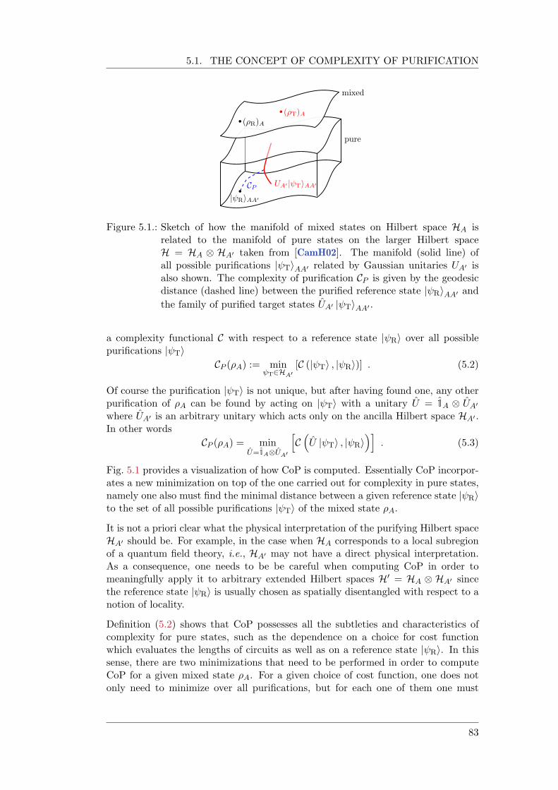
5.1. THE CONCEPT OF COMPLEXITY OF PURIFICATION
pure
UA |ψTiAACP
|ψRiAA
mixed
(ρR)A
(ρT)A
Figure 5.1.: Sketch of how the manifold of mixed states on Hilbert space HA isrelated to the manifold of pure states on the larger Hilbert spaceH = HA HA0 taken from [CamH02]. The manifold (solid line) ofall possible purifications | TiAA0 related by Gaussian unitaries UA0 isalso shown. The complexity of purification CP is given by the geodesicdistance (dashed line) between the purified reference state | RiAA0 and
the family of purified target states UA0 | TiAA0 .
a complexity functional C with respect to a reference state | Ri over all possiblepurifications | Ti
CP (A) := minψT2HA0
[C (| Ti , | Ri)] . (5.2)
Of course the purification | Ti is not unique, but after having found one, any otherpurification of A can be found by acting on | Ti with a unitary U = 1A UA0
where UA0 is an arbitrary unitary which acts only on the ancilla Hilbert space HA0 .In other words
CP (A) = minU=1AUA0
hCU | Ti , | Ri
i. (5.3)
Fig. 5.1 provides a visualization of how CoP is computed. Essentially CoP incorpor-ates a new minimization on top of the one carried out for complexity in pure states,namely one also must find the minimal distance between a given reference state | Rito the set of all possible purifications | Ti of the mixed state A.
It is not a priori clear what the physical interpretation of the purifying Hilbert spaceHA0 should be. For example, in the case when HA corresponds to a local subregionof a quantum field theory, i.e., HA0 may not have a direct physical interpretation.As a consequence, one needs to be be careful when computing CoP in order tomeaningfully apply it to arbitrary extended Hilbert spaces H0 = HA HA0 sincethe reference state | Ri is usually chosen as spatially disentangled with respect to anotion of locality.
Definition (5.2) shows that CoP possesses all the subtleties and characteristics ofcomplexity for pure states, such as the dependence on a choice for cost functionwhich evaluates the lengths of circuits as well as on a reference state | Ri. In thissense, there are two minimizations that need to be performed in order to computeCoP for a given mixed state A. For a given choice of cost function, one does notonly need to minimize over all purifications, but for each one of them one must
83
CHAPTER 5. COMPLEXITY OF PURIFICATION
also solve the problem of finding the optimal circuit. Moreover, one would need inprinciple to consider purifications with an arbitrary number of ancillae, as there isa priori no reason why minimal purifications, i.e., purifications whose ancilla havethe same number of degrees of freedom as the reduced density matrix, would be theoptimal or even sufficient to minimize complexity.
It is therefore to be expected that the efficient evaluation of CoP is in general achallenging task. The main reason being that generally the minimization proceduremust be done numerically, where the dimension of the manifold over which one mustperform the minimization grows rapidly with the number of degrees of freedom inHA. In order to make the study of CoP tractable, we will study CoP for Gaussianpurifications of mixed Gaussian states. That is, starting from a Gaussian mixedstate GA we will consider Gaussian purifications | Gi and then perform the minim-
ization only over Gaussian states UG | Gi where UG = 1A UGA0 is a unitary which
defines a family of Gaussian states. That is, we will focus on Gaussian complexityof purification
CGP (
GA) = min
UG=1AUGA0
hC(UG | Gi , | Ri)
i, (5.4)
which satisfies CP (GA) CG
P (GA). That is, the Gaussian CoP bounds the “true”CoP
from above. As we will see in Chap 6, there is numerical evidence that supports theconjectured equality for entanglement of purification EP (
GA) = EG
P (GA), although
this is not straightforward to verify in the case of CoP. However, studying CoPor in general complexity for non-Gaussian states remains a challenge and limitedprogress has been achieved on this front so far. It is therefore meaningful to restrictto Gaussian purifications of Gaussian mixed states.
In this case we will be able to use the machinery of the covariance matrix and linearcomplex structure formalism to Gaussian states described in detail in Sec. 3.2. Fora mixed Gaussian state A, its linear complex structure JA has purely imaginary ei-genvalues ±i ci, where ci 2 [1,1) and ci 2 [0, 1] for bosons and fermions respectively.A parametrization of these eigenvalues is ci = cosh(2ri) for bosons and ci = cos(2ri)for fermions. As we saw in (3.17), the Gaussian state will be pure in the case inwhich ci = 1 for all i. The general form of JA for a mixed Gaussian state GA in a
canonical basis aA = q1A, p1A, . . . , q
NA
A , pNA
A is given by
JA =
0B@
c1A2 0 0
0. . . 0
0 0 cNAA2
1CA where A2 =
0 11 0
, (5.5)
or equivalently
JA =
NAM
i=1
0 cici 0
. (5.6)
We can always find a basis aA0 = q1A0 , p1A0 , . . . , qNA0
A0 , pNA0
A0 such that the complex
84
5.1. THE CONCEPT OF COMPLEXITY OF PURIFICATION
structure J of a Gaussian purification | Gi of GA is given by [224]
J =
0BBBBBBBBBBBBBBB@
c1A2 · · · 0 s1S2 · · · 0 0 · · · 0...
. . ....
.... . .
......
. . ....
0 · · · cNAA2 0 · · · sNA
S2 0 · · · 0
±s1S2 · · · 0 c1A2 · · · 0 0 · · · 0...
. . ....
.... . .
......
. . ....
0 · · · ±sNAS2 0 · · · cNA
A2 0 · · · 0
0 · · · 0 0 · · · 0 A2 . . . 0
.... . .
......
. . ....
.... . .
...0 · · · 0 0 · · · 0 0 . . . A2
1CCCCCCCCCCCCCCCA
, (5.7)
where (+) and si =q
c2i 1 corresponds to bosons and () and si =q
1 c2i to
fermions, and where
S2 =
0 1
1 0
!. (5.8)
An equivalent parametrization of si in terms of ri, where si = sinh(2ri) for bosonsand si = sin(2ri) for fermions.
Here we have considered a purification with NA0 = NA + Nnm NA degrees offreedom, where Nnm corresponds to the number of additional ancillary degrees offreedom for a non-minimal purification. From (5.7) we see that in general the formof the linear complex structure J of the general Gaussian purification | Gi is
J =
JA JAA0
JA0A JA0
, (5.9)
which is of dimension (NA + NA0) (NA + NA0) = (2NA + Nnm) (2NA + Nnm).It is important to note that different purifications of GA only differ by the choice
of the basis of the purifying system A0, namely aA0 , for which J takes the standardform (5.7). Because of this, the action of the corresponding Lie group GA0 can beused to transform J !MJM1 withM = 1AMA0 where MA0 2 GA0 is representedby a (2NA0) (2NA0) matrix.
The next step is to identify the possible reference states |JRi that can be considered.Two straightforward choices are thermal states and mixed states arising from spatialsubsystems. In the latter case, which will be the focus of our approach, we startfrom a pure Gaussian state | i 2 H = HA HA which is then reduced to a localsubsystem A = trHA
(| i h |). In said subsystem, there is a pure and spatiallydisentangled Gaussian reference state |JRiA which can be extended to the purifyingsystem as |JRi = |JRiA |JRiA0 2 H0 = HA HA0 . In this case, only the targetstate |JTi is entangled in H0 = HA HA0 , while the reference state is a productstate |JRi = |JRiA |JRiA0 . Since there is a priori no physical notion of locality inthe ancillary system A0, as we mentioned previously, the only requirement is that|JRiA is pure and Gaussian. Hence, the natural choices for bosonic and fermionicreference states are:
JR =
NAM
i=1
0 1
µ
µ 0
, (bosons) (5.10a)
85
CHAPTER 5. COMPLEXITY OF PURIFICATION
JR =
NAM
i=1
0 11 0
, (fermions) (5.10b)
where here i denotes the local sites, and where here µ is the reference state scale orfrequency, as in (3.55).
Another consequence of our decision to focus on Gaussian states is that we canchoose the L2 cost function, which is the geodesic distance between Gaussian states|JTi and |JRi within the manifold of Gaussian states, as a measure of pure-statecomplexity in (5.4) and which is given by
C(|JTi , |JRi) =1
2p2
p|tr (log(G )2) | =
1
2p2
p|tr (log(JTJR)2) | , (5.11)
for G = JTJR, as in (3.58) and (3.93). Note that by construction the complexityfunctional (5.11) is invariant under the action of a Gaussian unitary U acting bothon the reference state and target state:
C(|JTi , |JRi) = C(U |JTi , U |JRi) , (5.12)
where U is related to a group transformation Mab 2 G via U †aU = Ma
bb. Con-
sequently, the optimization over all Gaussian purifications in (5.4) can be thereforeperformed over the reference or target state. As mentioned previously, we will optim-ize over all Gaussian purifications for the target state; having found one purification|JTi, any other purification is generated by unitaries of the form (1A UA0) |JTi.Hence
CP (|JTi , |JRi) = minUA0
hC(1A UA0) |JTi , |JRi
i
= minVA0
hCh(|JTi , (1A VA0) |JRi
i
= minUA0 ,VA0
hC(1A UA0) |JTi , (1A VA0) |JRi
i,
(5.13)
where UA0 and VA0 are both Gaussian unitaries acting only on the ancillary systemA0. This follows from (5.12). As a consequence, we can choose to begin with a basisaA such that (JT)A has the form (5.5) and then purify the system with respect to a
basis (0)a = (aA, aA0) so that JT takes the standard form (5.7) with respect to (0)a.
The purification of the reference state will then have the block diagonal form
JR = (JR)A (JR)A0 =
(JR)A 0
0 (JR)A0
, (5.14)
since it is a product state. For M = 1A MA0 we have (1A UA0) |Ji = |MJM1iso that
CP (JT, JR) = minM=1AMA0
"1
2p2
rtrlog (MJTM1JR)
2#
. (5.15)
By the cyclicity of the trace, this transformation on the target state can be equival-ently thought of as acting on the reference state via JR !M1JRM . This explicitly
86
5.1. THE CONCEPT OF COMPLEXITY OF PURIFICATION
shows our claim that we can choose to perform the optimization over the referencestate rather than on the target state. In practical terms, it is actually convenientto do this as the stabilizer group of the reference state is larger, leading to fewerparameters over which one must optimize.
Furthermore, let us emphasize that the L2 cost function (5.11) allows for a tractablecomputation of the complexity of purification given that the expressions for thepure-state Gaussian complexity both for bosonic and fermionic states are knownas a function of the reference and target states, as we saw in Sec. 3.3 (see (3.61)for bosons and (3.94) for fermions). For other cost functions, e.g., the L1, evenwithin the realm of Gaussian states, it would be necessary to optimize both overall purifications and over each purification it would be necessary to find the optimalcircuit connecting the reference and target states.
Having discussed the details of the Gaussian Cop, in Sec. 5.1.1 we will give an first ex-ample of CoP for a system of two coupled harmonic oscillators in the time-dependentsetting discussed in the previous chapter, namely that of a smooth quantum quenchthrough a critical point. This will set the stage for Sec. 5.2 where we will study CoPfor spatial subregions of vacuum states of the two (1+1)-dimensional free fermionicand bosonic quantum field theories that we described in Sec. 3.3.1 and Sec. 3.3.2,namely the Klein–Gordon and Ising CFT theories. In all cases we will also focuson minimal purifications Nnm = 0, given that a considerable amount of numericalevidence for the cost function (5.15) shows that adding additional ancillae does notlower the value of CoP.
While we do not possess at the moment a concrete mathematical argument in favourof minimal purifications, the reader should note that it is at least in principle possiblethat adding additional ancilla to general purifications could open the possibilityfor shorter circuits connecting the purified reference and target states. It wouldbe interesting to explore whether this observation is special to the choice of costfunction or if it’s a more general statement applicable to a larger class of complexitymeasures.
5.1.1. A Simple Model: Two Harmonic Oscillators
One of the simplest setups where one can study complexity of purification is thecase of a system comprised of two coupled harmonic oscillators. We begin with apure state describing the ground state of such system, which in position space ischaracterized by its wavefunction
(q1, q2) =
a1a2 a23
1/4p
exp!1
2q21
!2
2q22 !3q1q2
, (5.16)
where !i = ai + i bi and ai, bi 2 R such that ai > 0 and a1a2 > a23. The covariancematrix of the state (5.16) has the form:
G =
G11 G12
G21 G22
, (5.17)
where the blocks G12 and G21 describe the entanglement between the oscillators la-belled by 1 and 2 given by the cross-correlations q1p2 and q2p1. One can make
87
CHAPTER 5. COMPLEXITY OF PURIFICATION
a Fourier transform effectively performing a normal mode decomposition of theground state as in (3.46) arriving at a block diagonal structure of the covariancematrix (5.17). This indeed will be the strategy of Sec. 5.2.2 where we will study CoPof subsystems of N coupled harmonic oscillators corresponding to spatial subregionsof the vacuum state of the Klein–Gordon theory. However, it is also interesting forthe moment to remain in the basis a = q1, p1, q2, p2 in order to appreciate somefurther subtleties of CoP. We will thus follow the strategy of [CamH03].
From the pure state (5.16) we can obtain two mixed states corresponding to twosubsystems; each comprised of a single harmonic oscillator. The reduced densitymatrix corresponding to the first oscillator obtained simply by tracing out the secondoscillator 1 := tr2(| i h |) in position-space via
1(q1, q1) =
Z +1
1dq2
(q1, q2) (q1, q2) , (5.18)
is given by
1(q1, q1) =
r↵1
exp
1
2↵1(q
21 + q21)
i
2↵2(q
21 q21) + q1q1
, (5.19)
or equivalently 1(q1, q1) = exp(qaba1 b1 c0) as in (3.19) and where
↵1 = a1 a23 b232a2
, ↵2 = b1 +a3b3a2
, =a23 + b232a2
. (5.20)
Here the basis is a1 = q1, p1, q1, p1, c0 = log(/(↵1 ))/2 and
qab =
(↵1 + i↵2)/2 /2
/2 (↵1 i↵2)/2
. (5.21)
The reader should note that the three parameters ↵1,↵2, completely characterizethe covariance matrix G11, computed as in (3.18a), and linear complex structure J1corresponding to the first harmonic oscillator
G11 =
1
α1βα2
α1β
α2α1β
α21+α2
2β2
α1β
!, J1 =
α2
α1β 1
α1βα21+α2
2β2
α1β α2
α1β
!. (5.22)
Note that the parameter arising purely from the coupling between oscillators 1and 2 prevents the density matrix (5.19) from describing a pure state, as can be seenby computing the square of its linear complex structure
J21 =
α1+βα1β
0
0 α1+βα1β
!6= 12 . (5.23)
This can also be directly seen by noting that the covariance matrix of 1(q1, q1) (5.22)requires three parameters to be specified, as opposed to two, as would be in the caseof a pure state. This extra parameter arises from the entanglement between the twooscillators, namely from .
88
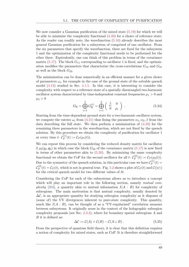
5.1. THE CONCEPT OF COMPLEXITY OF PURIFICATION
We now consider a Gaussian purification of the mixed state (5.19) for which we willbe able to minimize the complexity functional (4.33) for a choice of reference state.As the reader can readily note, the wavefunction (5.16) already describes the mostgeneral Gaussian purification for a subsystem of comprised of one oscillator. Fromthe six parameters that specify the wavefunction, three are fixed for the subsystem1 and the optimization of the complexity functional needs to be performed for theother three. Equivalently, one can think of this problem in terms of the covariancematrix (5.17). The block G11 corresponding to oscillator 1 is fixed, and the optimiz-ation modifies the parameters that characterize the cross-correlations G12 and G21
as well as the block G22.
The minimization can be done numerically in an efficient manner for a given choiceof parameters !i, for example in the case of the ground state of the solvable quenchmodel (4.13) studied in Sec. 4.1.1. In this case, it is interesting to consider thecomplexity with respect to a reference state of a spatially disentangled two-harmonicoscillator system characterized by time-independent constant frequencies µ1 > 0 andµ2 > 0
GR =2M
i=1
G(i)R =
2M
i=1
1µi
0
0 µi
. (5.24)
Starting from the time-dependent ground state for a two-harmonic oscillator system,we compute the entries !i from (4.21) thus fixing the parameters ↵1,↵2, from thedata describing the full state. We then perform a minimization of (4.33) for theremaining three parameters in the wavefunction, which are not fixed by the quenchsolution. By this procedure we obtain the complexity of purification for oscillator 1
at every time t: C(1)P (t) := CP (1(t)).
We can repeat this process by considering the reduced density matrix for oscillator2 2(q2, q2) in which case the block G22 of the covariance matrix (5.17) is now fixedin terms of other parameters akin to (5.20). By minimizing the same complexity
functional we obtain the CoP for the second oscillator for all t: C(2)P (t) := CP (2(t)).
Due to the symmetry of the quench solution, in this particular case we have C(1)P (t) =
C(2)P (t) = CP (t), which is not in general true. Fig. 5.2 shows a plot of CP (t) and C(| i)
for the critical quench model for two different values of t.
Considering the CoP for each of the subsystems allows us to introduce a conceptwhich will play an important role in the following section, namely mutual com-plexity [203], a quantity akin to mutual information I(A : B) for complexity ofsubregions. The main motivation is that mutual complexity, usually denoted by∆C, is an appropriate quantity for studying subregion complexity as it disposes of(some of) the UV divergences inherent to pure-state complexity. This quantity,much like I(A : B), can be thought of as a “UV-regularised” correlation measurebetween subsystems. It originally arose in the context of the holographic subregioncomplexity proposals (see Sec. 2.3.2), where for boundary spatial subregions A andB it is defined as:
∆C := C(A) + C(B) C(A [B) . (5.25)
From the perspective of quantum field theory, it is clear that this definition requiresa notion of complexity for mixed states, such as CoP. It is therefore straightforward
89
CHAPTER 5. COMPLEXITY OF PURIFICATION
t=10
t=1
-4 -2 0 2 4 6 8 100.2
0.4
0.6
0.8
1.0
1.2
1.4
t
C2(t)vsCP(t)
Figure 5.2.: Comparison of complexity of the pure target state C( ) as a functionof time t (solid) and the purification CP (dashed) for t = 10 (blue)and t = 1 (red), with µ1 = µ2 = 1/2 for both oscillators, taken from[CamH03].
to apply the notion of CoP to define the mutual complexity in terms of complexityof purification as
∆C(1)P := CP (A) + CP (B) CP (A[B) , (5.26)
where A and B are reduced density matrices corresponding to spatial subregionsA and B and where here CP (A[B) could be immediately replaced by C(| i h |) inthe case in which the union A[B coincides with the whole system defined by a purestate | i. We will focus on this notion of mutual complexity for the moment, butwe will in fact use an alternative one in Sec. 5.2 more adequate to eliminating theUV divergences which arise from an L2 norm.
It is also worth pointing out that one generally expects CoP to diverge in the con-tinuum limit as circuits acting on spatially disentangled states need to build entan-glement on all scales in order to match the features of vacuum states of free quantumfield theories, a fact which is also supported by explicit results such as [202]. There-fore, it is meaningful to consider a combination of CoP would cancel such divergenceswhile at the same time allowing to extract relevant physical information from thesubsystems.
Again from Fig. 5.2 we can see in this case that , for all t, CoP is smaller than the fullcomplexity but larger than half of it: C(| i)/2 CP (1,2) C(| i). This inequalitycan be also be numerically verified for a wide range of parameters independently ofthe quench solution. The inequality CP (1,2) C(| i) is saturated in the case inwhich the original target state is already the least complex state among all possiblepurifications. Meanwhile, the inequality C(| i)/2 CP (1,2) is saturated in the casewhere the original target state is a product state with respect to the chosen bipar-tition; i.e., if the subsystem of each individual oscillator is actually in a pure state.The previous inequality leads to the conjecture that complexity of purification forspatial subregions satisfies subadditivity CP (1) + CP (2) = 2 CP (1,2) C(| i).2 In
2Subadditivity can in general be defined for real-valued functions or set functions. In the lattercase, if R is a set and f : P (R) ! R is a set function, where P (R) denotes the power set of R,then f is said to be subadditive if for any S, T R we have f(S) + f(T ) f(S [ T ) 0.
90
5.2. VACUUM SUBREGIONS OF FREE QUANTUM FIELD THEORIES
other words,
∆C(1)P 0 . (5.27)
A striking consequence of this observation is that it contradicts the holographicsubregion proposals in Sec. 2.3.2, which are superadditive. We will explore morein detail the connection between these holographic proposals and the field theoreticproperties of bosonic and fermionic CoP in the following section.
It is also interesting to compare the complexity of purification C(1)P and entanglement
entropy S1 := tr(1 log(1)) for a single oscillator given by
S1(↵1,) =1
2
" 1
s↵1 +
↵1
!log
1
2
1
s↵1 +
↵1
!+ 1 +
s↵1 +
↵1
!log
1
2
1 +
s↵1 +
↵1
!
#.
(5.28)
Note that while C(1)P depends non-trivially on the parameter ↵2 of (5.19), as well as
the full state complexity C, S1 is insensitive to such parameter, which gives a hintas to how different information about the full state is encoded differently in entan-glement and complexity. For completeness one can also see that the entanglemententropy S1 goes to zero as the parameter which characterizes the entanglementbetween the two oscillators goes to zero.
Before moving on, the reader may also note how quickly this minimization procedureof the complexity functional can become computationally challenging as we increasethe number of degrees of freedom in the subsystem described by a Gaussian reduceddensity matrix. Already for a subsystem consisting of two harmonic oscillatorsdescribed by a reduced density matrix one would need to minimize a functional for10 parameters in the case of a minimal purification.3 If we are to make statementsabout CoP in quantum field theory we inevitably have to consider larger subsystems.This presents a challenging problem for which simplifying assumptions have beenconsidered recently, for example approximating the true CoP by a sum of single-mode optimizations of the complexity functional [202] or avoiding purifying themixed state all together [282, 283]. However, as we have already anticipated, byexploiting the natural structure of Gaussian pure and mixed states we are able toefficiently perform the optimization required to compute CoP in the case of Gaussianpurifications. This will be the focus of the next section, Sec. 5.2.
5.2. Vacuum Subregions of free Quantum Field Theories
In this section we will be interested in studying CoP for vacuum subregions of the(1+1)-dimensional Klein–Gordon model (see Sec. 3.3.1) and of the critical transverseIsing model (see Sec. 3.3.2). We will present the results of numerical computations
3For a bosonic system or subsystem described by N degrees of freedom, the dimension of themanifold of pure Gaussian states with vanishing one-point functions is N(N + 1), while thedimension of the manifold of mixed Gaussian states with vanishing one-point functions isN(2N+1) [221].
91
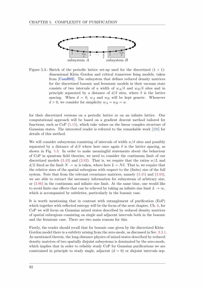
CHAPTER 5. COMPLEXITY OF PURIFICATION
d
δ
. . .1 1 . . . wB
δwA
δ
. . .1
subsystem A subsystem B
Figure 5.3.: Sketch of the periodic lattice set-up used for the discretized (1 + 1)-dimensional Klein–Gordon and critical transverse Ising models, takenfrom [CamH02]. The subsystem that defines reduced density matricesfor the discretized bosonic and fermionic models in their vacuum stateconsists of two intervals of a width of wA/ and wB/ sites and inprinciple separated by a distance of d/ sites, where is the latticespacing. When d = 0, wA and wB will be kept generic. Wheneverd > 0, we consider for simplicity wA = wB = w.
for their discretized versions on a periodic lattice or on an infinite lattice. Ourcomputational approach will be based on a gradient descent method tailored forfunctions, such as CoP (5.15), which take values on the linear complex structure ofGaussian states. The interested reader is referred to the remarkable work [226] fordetails of this method.
We will consider subsystems consisting of intervals of width w/ sites and possiblyseparated by a distance of d/ where here once again is the lattice spacing, asshown in Fig. 5.3. In order to make meaningful statements about the behaviourof CoP in quantum field theories, we need to consider the continuum limit of ourdiscretized models (3.43) and (3.82). That is, we require that the ratios w/L andd/L fixed as the limit N !1 is taken, where here L = N. That is, we require thatthe relative sizes of the spatial subregions with respect to the (finite) size of the fullsystem. Note that from the relevant covariance matrices, namely (3.45) and (3.83),we are able to extract the necessary information for subsystems of arbitrary size,or (3.86) in the continuum and infinite size limit. At the same time, one would liketo avoid finite size effects that can be relieved by taking an infinite size limit L!1,which is accompanied by subtleties, particularly in the bosonic case.
It is worth mentioning that in contrast with entanglement of purification (EoP)which together with reflected entropy will be the focus of the next chapter, Ch. 6, forCoP we will focus on Gaussian mixed states described by reduced density matricesof spatial subregions consisting on single and adjacent intervals both in the bosonicand the fermionic case. There are two main reasons for this.
Firstly, the reader should recall that for bosonic case given by the discretized Klein–Gordon model there is a subtlety arising from the zero-mode, as discussed in Sec. 3.3.1.As mentioned therein, the long-distance physics of mixed states described by reduceddensity matrices of two spatially disjoint subsystems is dominated by the zero-mode,which implies that in order to reliably study CoP for Gaussian purifications we areconstrained in principle to study single, adjacent (d = 0) or disjoint intervals sep-
92
5.2. VACUUM SUBREGIONS OF FREE QUANTUM FIELD THEORIES
arated by a short distance d w. For the latter case, however, we would need toconsider subsystem sizes consisting of a large number of lattice sites w/ of order> O(10) in order to properly characterize CoP as a function of d/w in the con-tinuum limit while at the same time avoiding finite size effects occurring for smallseparations d/ O(1). Precise numerical computations for such cases are partic-ularly challenging due to the dimension of the parameter manifold over which theoptimization needs to be performed.
To give an example, consider the case for which d/w O(1/10), which arguablysatisfies the condition d w. Suppose for example that the separation betweenthe subsystems is d/ O(3 4) lattice sites in order to avoid finite size effects.This implies that the subsystems should have a size of at least w/ O(30 40)lattice sites, implying that the number of degrees of freedom of the reduced densitymatrix for this subsystem is NA = 2w O(60 80), for which the manifold ofGaussian purifications will be of dimension 2NA(2NA + 1) O(3660 6480) andwhere the optimization should be performed in principle for a subspace of dimensionNA(2NA + 1) O(1830 3240).
At the moment, exploratory computations in this regime yield a behaviour of mutualCoP (5.26) in the continuum limit N !1 for a small d/w range given by
∆C(1)P (d/w,m/µ, µ)
dw
f(m/µ, µ) log(d/w) + · · · , (5.29)
where the precise form of the function f(m/µ, µ) as well as the character of sublead-
ing contributions to (∆C(1)P )dw has not been fully determined. As a consequence,
we leave the details of the d > 0 case for bosonic CoP for the future and outside thescope of the present work.
The second reason is related with the notion of locality in the Ising CFT and thenon-Gaussian nature of the reduced density matrix for disjoint subsystems. Thebasic idea, as discussed already in Sec. 3.3.2, is that there are different notions oflocality in the spin and fermion pictures which lead to a different notion of partialtrace in lattice systems with a Jordan–Wigner duality [284]. This leads in particularto a different notion of entanglement entropy in the two pictures, a fact has alreadybeen recognised in the literature [237, 238, 285–287] and which plays a substantialrole when relating the lattice model with the continuum CFT [240]. However, thisdifferent notion only affects disjoint subregions, i.e., mixed states whose reduceddensity matrix describes a subsystem consisting of two non-adjacent intervals. Thisfact constrains us to consider only single and adjacent intervals d = 0 in Fig. 5.3,of the Ising CFT model. In Sec. 6.3, however, we will return to the study of thelong-distance behaviour of two quantities of interest, namely of entanglement ofpurification and reflected entropy.
It would be remiss not to address the CFT limit of both discretized models. Inthe bosonic case, this limit is naively achieved by taking m ! 0 which leads to aconformal field theory with central charge c = 1. However to be precise, the masslesslimit of the Hamiltonian (3.41) actually corresponds to the decompactification limitof a one-parameter family of compact free boson conformal field theories arisingfrom the compactification of the bosonic field ' and which has corresponds to a
93
CHAPTER 5. COMPLEXITY OF PURIFICATION
different conformal field theory with a different partition function than the modular-invariant c = 1 CFT. This difference can be understood by studying the zero-modecontribution to the path-integral. While distinct, we will use our discretized modelof a free massive boson as a proxy for extracting the properties of CoP for themodular invariant c = 1 free boson conformal field theory in the regimes for whichthe zero-mode is subdominant namely for single and adjacent intervals. One couldalso in principle study the regime d w without worrying too much about the zeromode. The reader can refer to [CamH02] where a thorough discussion of the CFTlimit of both discretized models is made, as well as of the zero-mode problem and theinequivalent notions of partial trace and tensor product under the Jordan–Wignerduality for lattice spin systems.
As a final comment before proceeding to the following sections, it is worth pointingout that given that our choice of cost function (5.15) is based on an L2 norm whichhas a square root, it makes sense to consider a variation of the mutual complex-ity formula (5.26) more appropriate to dispose of the UV divergencies inherent tocomplexity, namely (3.63) and (3.96). We propose the L2 mutual complexity forreduced density matrices A and B corresponding to subregions A and B to bedefined by
∆C(2)P := CP (A)
2 + CP (B)2 CP (A[B)
2 , (5.30)
where here the (2) on the superscript on the left hand side does not signify a square,but rather simply that it is based on taking the square of individual contributionsand then adding them.
5.2.1. Fermionic Complexity of Purification
We begin with the study of the fermionic case as it is far simpler than the bosonicone mainly due to the fact that there are fewer parameters. In particular, there is noreference state scale associated to the reference state. As we mentioned previously,see e.g., the paragraph preceding (3.89), in contrast with the bosonic case, fermi-onic reference states are highly constrained as there exists only a single spatiallyunentangled state with the same parity as the vacuum state which is translationalinvariant.
For a single interval on a line, fermionic CoP can only be a function of the ratio w/as the system becomes large N !1. In this limit, fermionic CoP behaves as
C2P = e2
w
+ e1 log
w
+ e0 , (5.31)
where the ei are numerical coefficients which can be determined up to the accuracypermitted by the optimization algorithm and which are found to be
e0 = 0.0894 , e1 = 0.0544 , e2 = 0.103 . (5.32)
This functional form (5.31) was tested numerically by computing discrete derivativesof C2
P with respect to w/. Note that in (5.31) we are directly considering the squareof the CoP.
Formula (5.31) for fermionic CoP matches the structure of leading divergence forvacuum complexity in free fermionic conformal field theories [204, 205] and also in
94
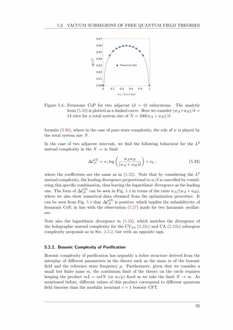
5.2. VACUUM SUBREGIONS OF FREE QUANTUM FIELD THEORIES
Numerical data
0 0.2 0.4 0.6 0.8 1.
0.00
0.01
0.02
0.03
0.04
0.05
0.06
0.07
wA / (wA+wB)CP2
Figure 5.4.: Fermionic CoP for two adjacent (d = 0) subsystems. The analyticform (5.33) is plotted as a dashed curve. Here we consider (wA+wB)/ =14 sites for a total system size of N = 100(wA + wB)/.
formula (3.96), where in the case of pure state complexity, the role of w is played bythe total system size N .
In the case of two adjacent intervals, we find the following behaviour for the L2
mutual complexity in the N !1 limit
∆C(2)P = e1 log
wAwB
(wA + wB)
+ e0 , (5.33)
where the coefficients are the same as in (5.32). Note that by considering the L2
mutual complexity, the leading divergence proportional to w/ is cancelled by consid-ering this specific combination, thus leaving the logarithmic divergence as the leading
one. The form of ∆C(2)P can be seen in Fig. 5.4 in terms of the ratio wA/(wA +wB),
where we also show numerical data obtained from the optimization procedure. It
can be seen from Fig. 5.4 that ∆C(2)P is positive, which implies the subadditivity of
fermionic CoP, in line with the observation (5.27) made for two harmonic oscillat-ors.
Note also the logarithmic divergence in (5.33), which matches the divergence ofthe holographic mutual complexity for the CV2.0 (2.23c) and CA (2.23b) subregioncomplexity proposals as in Sec. 2.3.2, but with an opposite sign.
5.2.2. Bosonic Complexity of Purification
Bosonic complexity of purification has arguably a richer structure derived from theinterplay of different parameters in the theory such as the mass m of the bosonicfield and the reference state frequency µ. Furthermore, given that we consider asmall but finite mass m, the continuum limit of the theory on the circle requireskeeping the product mL = mN (or m/µ) fixed as we take the limit N ! 1. Asmentioned before, different values of this product correspond to different quantumfield theories than the modular invariant c = 1 bosonic CFT.
95
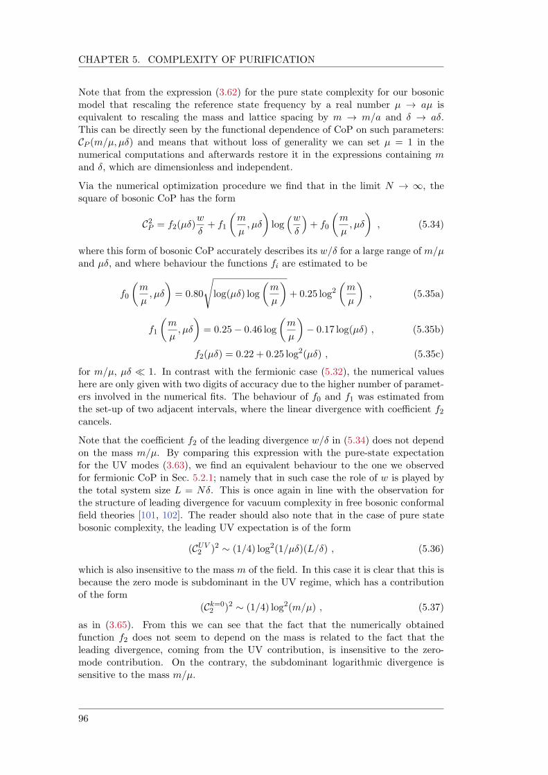
CHAPTER 5. COMPLEXITY OF PURIFICATION
Note that from the expression (3.62) for the pure state complexity for our bosonicmodel that rescaling the reference state frequency by a real number µ ! aµ isequivalent to rescaling the mass and lattice spacing by m ! m/a and ! a.This can be directly seen by the functional dependence of CoP on such parameters:CP (m/µ, µ) and means that without loss of generality we can set µ = 1 in thenumerical computations and afterwards restore it in the expressions containing mand , which are dimensionless and independent.
Via the numerical optimization procedure we find that in the limit N ! 1, thesquare of bosonic CoP has the form
C2P = f2(µ)
w
+ f1
m
µ, µ
log
w
+ f0
m
µ, µ
, (5.34)
where this form of bosonic CoP accurately describes its w/ for a large range of m/µand µ, and where behaviour the functions fi are estimated to be
f0
m
µ, µ
= 0.80
slog(µ) log
m
µ
+ 0.25 log2
m
µ
, (5.35a)
f1
m
µ, µ
= 0.25 0.46 log
m
µ
0.17 log(µ) , (5.35b)
f2(µ) = 0.22 + 0.25 log2(µ) , (5.35c)
for m/µ, µ 1. In contrast with the fermionic case (5.32), the numerical valueshere are only given with two digits of accuracy due to the higher number of paramet-ers involved in the numerical fits. The behaviour of f0 and f1 was estimated fromthe set-up of two adjacent intervals, where the linear divergence with coefficient f2cancels.
Note that the coefficient f2 of the leading divergence w/ in (5.34) does not dependon the mass m/µ. By comparing this expression with the pure-state expectationfor the UV modes (3.63), we find an equivalent behaviour to the one we observedfor fermionic CoP in Sec. 5.2.1; namely that in such case the role of w is played bythe total system size L = N. This is once again in line with the observation forthe structure of leading divergence for vacuum complexity in free bosonic conformalfield theories [101, 102]. The reader should also note that in the case of pure statebosonic complexity, the leading UV expectation is of the form
(CUV2 )2 (1/4) log2(1/µ)(L/) , (5.36)
which is also insensitive to the mass m of the field. In this case it is clear that this isbecause the zero mode is subdominant in the UV regime, which has a contributionof the form
(Ck=02 )2 (1/4) log2(m/µ) , (5.37)
as in (3.65). From this we can see that the fact that the numerically obtainedfunction f2 does not seem to depend on the mass is related to the fact that theleading divergence, coming from the UV contribution, is insensitive to the zero-mode contribution. On the contrary, the subdominant logarithmic divergence issensitive to the mass m/µ.
96
5.2. VACUUM SUBREGIONS OF FREE QUANTUM FIELD THEORIES
m = 10-2, = 10-2
m = 10-2, = 10-4
m = 10-4, = 10-2
m = 10-4, = 10-4
0.0 0.2 0.4 0.6 0.8 1.00
10
20
30
40
wA / (wA+wB)
CP2
Figure 5.5.: Bosonic CoP for two adjacent (d = 0) subsystems in units of the ref-erence state frequency µ = 1. The analytic form (5.38) is plotted asa dashed curve for different values of m . The numerical data is alsoshown. Here we consider (wA +wB)/ = 20 sites for a total system sizeof N = 100(wA + wB)/.
In the case of two adjacent intervals we use the single interval expression (5.34) toobtain the expression for mutual bosonic CoP
∆C(2)P = f1
m
µ, µ
log
wAwB
(wA + wB)
+ f0
m
µ, µ
, (5.38)
from which we can see that the leading divergence cancels, as expected, leaving thelogarithmic divergence as the leading one. Furthermore, the coefficients f0 and f1are the same as in the single interval case. Fig. 5.5 shows the behaviour of mutualbosonic CoP in terms of wA/(wA + wB). From Fig. 5.5 the reader can see thatas well as in the fermionic case, mutual complexity of purification is subadditive
∆C(2)P 0, which is also consistent with our observation (5.27) for two harmonic
oscillators.
Finally, note that the logarithmic divergence (5.38) also matches the divergence ofthe holographic mutual complexity for the CV2.0 (2.23c) and CA (2.23b) subregioncomplexity proposals as in Sec. 2.3.2, but just as the fermionic CoP result (5.33) ithas the opposite sign.
5.2.3. Comparison of bosonic CoP with other methods
In the previous section we presented the results for bosonic complexity of purifica-tion which were obtained via an optimization algorithm based on a steepest-descentmethod using the most general Gaussian purifications for mixed Gaussian states. Inorder to efficiently perform the minimization of the complexity functional, the nat-ural geometric structure of Gaussian states was crucial, which in the bosonic casearises from the manifold of symplectic transformations G =Sp(2N,R).
As we discussed, while this general method provides an accurate result for the result-ing CoP, it is not insensitive to computational difficulties associated with considering
97
CHAPTER 5. COMPLEXITY OF PURIFICATION
subsystems with a large number of degrees of freedom. A natural question whicharises in this case is whether we can translate the problem of finding the CoP for asystem with NA degrees of freedom, into the problem of finding CoP for NA systemswith a single degree of freedom.
This is the strategy that authors in [202] used to approximate the complexity ofpurification for single degrees of freedom of certain Gaussian states using an L1
norm arising from an F1 cost function (3.8a) derived originally for similar set-upsin [102]. In this work, authors define two types of L1 bases with which they performthe minimization of the geodesic distance with respect to an L2 norm since, as wementioned in Sec.(3.1.1), it is challenging to minimize the length of a path withrespect to a L1 norm, specially for several modes.
A key feature of subsystems of the Klein–Gordon model consisting several modes isthat it is in general not sufficient to optimize over individual modes in order to obtainthe true Gaussian CoP. The reason being that it is generally not possible to bringboth the (JT)A of a mixed Gaussian state A describing a subregion of the vacuumand the (JR)A of a spatially unentangled product state simultaneously into block-diagonal form. However, there may be cases in which the standard decompositionof the mixed target state also approximately decomposes the reference state intoindividual modes.
To see this, consider a single bosonic mode in the case of pure Gaussian refer-ence state and a mixed Gaussian target state which do not have ' -correlations.This is a more restricted setup compared with the two-harmonic oscillator casethat we studied in Sec. 5.1.1 for which we assumed in general non-vanishing ' -correlations.
This subsystem can be extended to a subsystem consisting of two bosonic modesH0 = HA HA0 with extended reference state |JRi and purified target state |JTisuch that their respective linear complex structures are given by
JT =
0BBBB@
0 0p2 1
0p2 1 0
0p2 1 0 p
2 1 0 0
1CCCCA
, (5.39a)
JR =
0BBB@
0 1µ 0 0
µ 0 0 0
0 0 0 1ν
0 0 0
1CCCA , (5.39b)
where 2 [1,1) is equivalent to the parameters ci for several degrees of freedom asin (5.6), µ is the reference state frequency for the original single bosonic mode and is a parameter for the extender reference state over which the minimization of thecomplexity functional (5.15) has to be performed. In this case, the L2 complexityfunctional has the form
C(, µ, ) =1
2
slog2
!+
µ
+ log2
!µ
, (5.40)
98
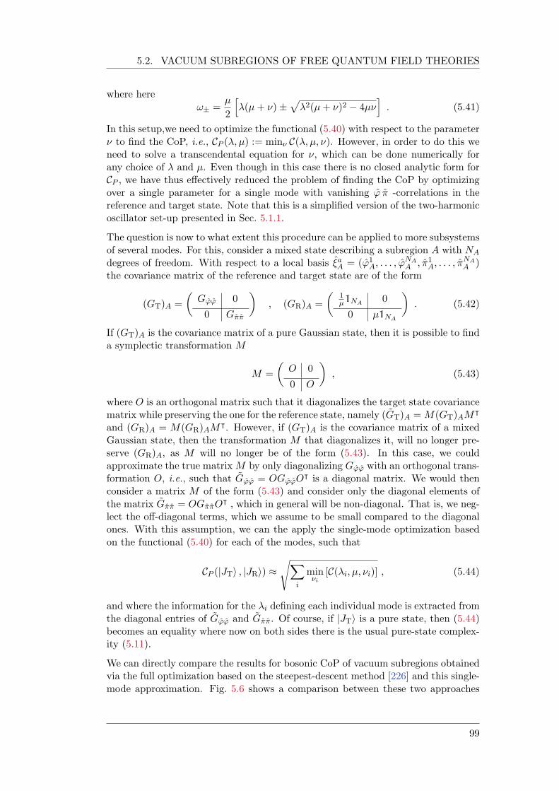
5.2. VACUUM SUBREGIONS OF FREE QUANTUM FIELD THEORIES
where here
!± =µ
2
h(µ+ )±
p2(µ+ )2 4µ
i. (5.41)
In this setup,we need to optimize the functional (5.40) with respect to the parameter to find the CoP, i.e., CP (, µ) := minν C(, µ, ). However, in order to do this weneed to solve a transcendental equation for , which can be done numerically forany choice of and µ. Even though in this case there is no closed analytic form forCP , we have thus effectively reduced the problem of finding the CoP by optimizingover a single parameter for a single mode with vanishing ' -correlations in thereference and target state. Note that this is a simplified version of the two-harmonicoscillator set-up presented in Sec. 5.1.1.
The question is now to what extent this procedure can be applied to more subsystemsof several modes. For this, consider a mixed state describing a subregion A with NA
degrees of freedom. With respect to a local basis aA = ('1A, . . . , '
NA
A , 1A, . . . , NA
A )the covariance matrix of the reference and target state are of the form
(GT)A =
Gϕϕ 0
0 Gππ
, (GR)A =
1µ1NA
0
0 µ1NA
. (5.42)
If (GT)A is the covariance matrix of a pure Gaussian state, then it is possible to finda symplectic transformation M
M =
O 0
0 O
, (5.43)
where O is an orthogonal matrix such that it diagonalizes the target state covariancematrix while preserving the one for the reference state, namely (GT)A = M(GT)AM
|
and (GR)A = M(GR)AM|. However, if (GT)A is the covariance matrix of a mixed
Gaussian state, then the transformation M that diagonalizes it, will no longer pre-serve (GR)A, as M will no longer be of the form (5.43). In this case, we couldapproximate the true matrix M by only diagonalizing Gϕϕ with an orthogonal trans-formation O, i.e., such that Gϕϕ = OGϕϕO
| is a diagonal matrix. We would thenconsider a matrix M of the form (5.43) and consider only the diagonal elements ofthe matrix Gππ = OGππO
| , which in general will be non-diagonal. That is, we neg-lect the off-diagonal terms, which we assume to be small compared to the diagonalones. With this assumption, we can the apply the single-mode optimization basedon the functional (5.40) for each of the modes, such that
CP (|JTi , |JRi) sX
i
minνi
[C(i, µ, i)] , (5.44)
and where the information for the i defining each individual mode is extracted fromthe diagonal entries of Gϕϕ and Gππ. Of course, if |JTi is a pure state, then (5.44)becomes an equality where now on both sides there is the usual pure-state complex-ity (5.11).
We can directly compare the results for bosonic CoP of vacuum subregions obtainedvia the full optimization based on the steepest-descent method [226] and this single-mode approximation. Fig. 5.6 shows a comparison between these two approaches
99
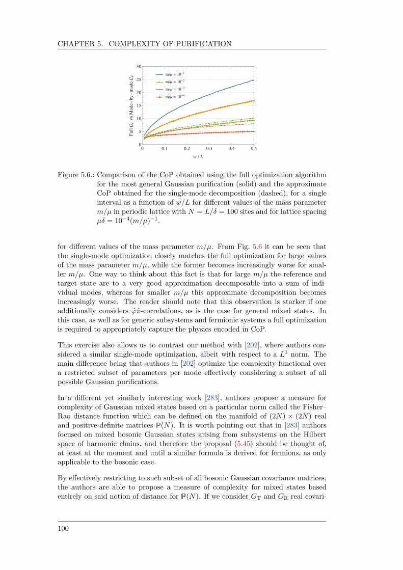
CHAPTER 5. COMPLEXITY OF PURIFICATION
m/ = 10-1
m/ = 10-2
m/ = 10-3
m/ = 10-4
0 0.1 0.2 0.3 0.4 0.50
5
10
15
20
25
30
w / L
Full
PvsMode-by-mode
P
Figure 5.6.: Comparison of the CoP obtained using the full optimization algorithmfor the most general Gaussian purification (solid) and the approximateCoP obtained for the single-mode decomposition (dashed), for a singleinterval as a function of w/L for different values of the mass parameterm/µ in periodic lattice with N = L/ = 100 sites and for lattice spacingµ = 104(m/µ)1.
for different values of the mass parameter m/µ. From Fig. 5.6 it can be seen thatthe single-mode optimization closely matches the full optimization for large valuesof the mass parameter m/µ, while the former becomes increasingly worse for smal-ler m/µ. One way to think about this fact is that for large m/µ the reference andtarget state are to a very good approximation decomposable into a sum of indi-vidual modes, whereas for smaller m/µ this approximate decomposition becomesincreasingly worse. The reader should note that this observation is starker if oneadditionally considers '-correlations, as is the case for general mixed states. Inthis case, as well as for generic subsystems and fermionic systems a full optimizationis required to appropriately capture the physics encoded in CoP.
This exercise also allows us to contrast our method with [202], where authors con-sidered a similar single-mode optimization, albeit with respect to a L1 norm. Themain difference being that authors in [202] optimize the complexity functional overa restricted subset of parameters per mode effectively considering a subset of allpossible Gaussian purifications.
In a different yet similarly interesting work [283], authors propose a measure forcomplexity of Gaussian mixed states based on a particular norm called the Fisher–Rao distance function which can be defined on the manifold of (2N) (2N) realand positive-definite matrices P(N). It is worth pointing out that in [283] authorsfocused on mixed bosonic Gaussian states arising from subsystems on the Hilbertspace of harmonic chains, and therefore the proposal (5.45) should be thought of,at least at the moment and until a similar formula is derived for fermions, as onlyapplicable to the bosonic case.
By effectively restricting to such subset of all bosonic Gaussian covariance matrices,the authors are able to propose a measure of complexity for mixed states basedentirely on said notion of distance for P(N). If we consider GT and GR real covari-
100
5.2. VACUUM SUBREGIONS OF FREE QUANTUM FIELD THEORIES
m/ = 10-1
m/ = 10-2
m/ = 10-3
m/ = 10-4
0 0.1 0.2 0.3 0.4 0.50
5
10
15
20
25
30
w / L
Pvsd(G,G0)
m/ = 10-3 , = 1/140
m/ = 10-4 , = 1/14
m/ = 10-5 , = 10/14
0 0.2 0.4 0.6 0.8 1.-15
-10
-5
0
5
10
15
wA / (wA+wB)
CP2vsd(G,G0)
Figure 5.7.: Comparison of CoP obtained using the Gaussian optimization algorithm(solid) and the Fisher–Rao distance function (dashed) for a single in-terval (top) and two adjacent intervals (bottom). The data for thesingle interval case were generated for a mass parameter m/µ =101, 102, 103, 104, N = L/ = 100, and for lattice spacing µ =104(m/µ)1, while the data for the adjacent interval case were gener-ated for a mass parameter m/µ = 103, 104, 105, N = L/ = 1400,(wA + wB) = 14, and for lattice spacing µ = (1/14) 104(m/µ)1.
ance matrices for mixed target and reference Gaussian states, then the Fisher–Raodistance function
d(GT, GR) =1
2p2
qtrlog2(GTG
1R )
, (5.45)
which measures the geodesic distance between the two matrices is interpreted asthe complexity of one state with respect to the other. Fig. 5.7 shows a comparisonbetween the CoP obtained with the full optimization algorithm and the Fisher–Raodistance function (5.45). From it we can see that for the case of a single intervalthere is both a quantitative and qualitative agreement between both notions, whereasfor the two adjacent intervals these deviate notable and significantly although thequalitative behaviour remains comparable.
It is also interesting to note that the single-interval agreement is particularly remark-able, given the fact that these two notions are distances defined on different spaces.While CoP is defined as the geodesic distance between purified reference and targetstates on an enlarged Hilbert space H0 = HA HA0 , as can be seen in Fig. 5.1, theFisher–Rao distance function is a measure defined entirely on the manifold of mixed
101
CHAPTER 5. COMPLEXITY OF PURIFICATION
states associated with the Hilbert space HA, and in principle these needn’t even becomparable to each other.
5.3. Discussion
In this Chapter we discussed complexity of purification (CoP) for vacuum subregionsof (1 + 1)-dimensional free conformal field theories. We focused on two particularset-ups; one related to the discussion of Chapter 4 of complexity in non-equilibriumquantum dynamics, and one related to the study of CoP in subsystems comprisedof single and two adjacent intervals in the vacuum of lattice discretizations of freebosonic and fermionic theories. In both cases we exploited the Gaussian character ofthe mixed states in consideration to use the full machinery of Gaussian techniquesof Chapter 3 in order to study CoP.
In the first set-up, we studied CoP for a subsystem comprised of two harmonic oscil-lators with a time dependent mass, following Chapter 4. This simple yet revealingset-up allowed us to present the concept of CoP while at the same time provid-ing evidence for the sub-additivity of mutual complexity, a UV-regulated quantityakin to mutual information adequate for studying the CoP for bipartite subsystems.Furthermore, this set-up provided an example to the known claim in the AdS/CFTcorrespondence that“entanglement entropy is not enough”to capture the full inform-ation about a quantum system (which has a gravitational dual). We showed this bycomparing the functional dependence of entanglement entropy with the complexityof purification of a single oscillator.
In the second set-up, we studied CoP for vacuum subregions of free CFTs consistingof a single and two adjacent intervals. In the first case, we found that the leadingdivergence of CoP is a direct generalization of the leading divergence of pure-statecomplexity, which was studied in Chapter 3. We also found a subleading logar-ithmic divergence as well as a third term, which in the fermionic case is a simpleconstant, but in the bosonic case is a logarithmic divergence corresponding to thezero-mode.
For two adjacent intervals, we found a logarithmic divergence of the mutual com-plexity in both fermionic and bosonic models, which matches the holographic ex-pectation of the subregion complexity CA and CV2.0 proposals, though with theopposite sign. In the fermionic case, we find a simple characterization of the log-arithmic divergence with a constant coefficient, while in the bosonic case we find acoefficient with a complex interplay between different parameters such as the massand reference scales. This contradiction between the subadditive and superadditivebehaviours of subregion complexity from QFT and holography has been noticed be-fore (see e.g., [202]), but this is the first time that a full comparison between bothquantities has been done for both fermions and bosons, especially using the mostgeneral Gaussian purifications.
We also compared our approach and results for bosonic CoP with two recently-developed methods that have been used to study it, namely mode-by-mode purific-ations and the Fisher–Rao distance proposal. For the first method, we found thatour approach based on an optimization over the full Gaussian manifold provides
102
5.3. DISCUSSION
a better minimization of the complexity functional particularly when the theory istaken closer to criticality. This implies that the mode-by-mode approximation isinsufficient to accurately capture the behaviour of CoP in the critical theory. Forthe second one, we found that while the Fisher–Rao distance function appears tobehave similarly to the full CoP, the “mutual Fisher–Rao distance” seems to violatesubadditivity in some cases. Furthermore, this mixed-state proposal is only definedfor bosonic Gaussian states, as the positive-definiteness of the covariance matrix isnecessary for the implementation of the distance measure.
As a consequence, there are two main novelties of the results presented in thisChapter. Firstly, we provided results using a general optimization method for CoPfor any Gaussian mixed state in the vacuum of a CFT and showed that the mu-tual complexity computed via it has an equivalent logarithmic divergence akin totwo of the holographic subregion complexity proposals but is subadditive instead ofsuperadditive. We also showed that said method leads to an optimal minimizationof complexity which is stable and efficient also near criticality. As a consequence,these studies lay the foundation for a more complete understanding of CoP in freeCFTs.
103

CHAPTER 5. COMPLEXITY OF PURIFICATION
104
6. Entanglement of Purification and Reflected Entropy
In this chapter we present the study of entanglement of purification (EoP), a correl-ation measure which generalizes the notion of entanglement entropy to mixed states,and of reflected entropy (RE), another correlation measure built from the so-calledcanonical purification; both conjectured to be holographically dual to the entangle-ment wedge cross section (see Sec. 2.2.1). We introduce both notions in Sec. (6.1)and briefly discuss them. In Sec. 6.2.1 we focus entirely on Gaussian EoP, anddiscuss its behaviour for vacuum subregions of free quantum field theories (QFT)consisting of two adjacent intervals using the most general Gaussian purifications,following Sec. 3.3.1 and Sec. 3.3.2. We show that in both cases Gaussian EoP has aleading behaviour proportional to half the mutual information (MI) in accordancewith holographic and CFT expectations. In Sec. 6.2.2 we study bosonic GaussianEoP for disjoint intervals in the small separation regime, showing an agreement bothwith holographic and CFT expectations. Then in Sec. 6.3 we study EoP and RE fortwo largely-separated spherical subregions in the vacuum of a CFT in any dimen-sion with a gape in the operator spectrum. Using general arguments applicable tolattice realizations of said theories, we provide a proof that both quantities presenta logarithmic enhancement with respect to the leading power-law divergence in theseparation of the subregions, a feature which provides new insights into the largedistance behaviour of these correlation measures. Finally, using the c = 1/2 IsingCFT as a concrete example of a lattice model, we explicitly compute the overallcoefficients for both quantities.
6.1. The Concept of Entanglement of Purification and ReflectedEntropy
Quantifying the entanglement properties of quantum many-body systems is a chal-lenging and vast enterprise in quantum information science (see e.g., [288–291]).Of the several entanglement measures which can be defined, however, entanglemententropy (EE) stands out as arguably one of the most studied ones in the field ofhigh-energy physics. From quantum field theory (see [86, 228, 292, 293]), to con-formal field theory (see [294]) and the AdS/CFT correspondence (see [132, 227, 229]),quantum entanglement and the entropy associated with it has played a key role inthe development of the field over the past twenty years. See e.g., [229, 295] forrecent reviews.
In essence, EE is a measure of pure state entanglement between a subregion andits complement. Given a system in a pure quantum state described by a densitymatrix = | i h | and a subsystem A with reduced density matrix A = trA(), EEis defined as the von Neumann entropy of A
SA = S(A) := trA(A log(A)) , (6.1)
105
CHAPTER 6. ENTANGLEMENT OF PURIFICATION AND REFLECTEDENTROPY
where A denotes the complement of A. One can think of EE as measuring howentangled subsystem A is with its complement A in the state . In quantumfield theories, EE is an UV-divergent quantity due to correlations at arbitrarilyshort distances and its computation is in general a difficult task. However, sev-eral results are known in a variety of settings such as free theories [221, 296–299], two-dimensional CFTs [85, 300–303], two-dimensional gapped and gapless sys-tems [76, 88] and strongly-coupled holographic QFTs [118, 123, 127, 128].
For subsystems consisting of two components A[B, i.e., for bipartite Hilbert spacesH = HA HB, a quantity known as mutual information (MI) defined through EEas
I(A : B) := SA + SB SA[B , (6.2)
is used to characterize the correlations between them in a given pure state . MIhas the property of being a UV-regulated version of EE in quantum field theoriesand is therefore adequate for studying the correlations of bipartite spatial subre-gions. It should also be noted that in conformal field theories, MI is genericallynon-universal, as it is computed via a 4-point function of twist operators, which isspectrum dependent [86].
Note that the definition of entanglement entropy SA of a subregion A (6.1) intrinsic-ally requires the knowledge of the pure state = | i h | of which the subregion char-acterized by the reduced density matrix A is a subsystem of. The natural questionthen arises: how can we characterize the correlations between different componentsof a subsystem corresponding to a mixed state characterized by a reduced densitymatrix?
Of the correlation measures that can be defined for mixed states, two stand outin the context of the AdS/CFT correspondence, namely entanglement of purific-ation (EoP) and reflected entropy (RE).1 While EoP can be considered a mixedstate generalization of EE measuring the correlations of bipartite subsystems, REarises from an algebraic construction as the von Neumann entropy of the canonicalpurification of the mixed state describing the bipartite subsystem. Remarkably, inthe case of strongly-interacting QFTs with a holographic dual, both notions havebeen conjectured to be dual to the same gravitational quantity, namely the entangle-ment wedge cross section EW (see Sec. 2.2.1). As a consequence, contrasting thesetwo notions in conformal field theories can help elucidate their precise role in theAdS/CFT correspondence and their connection with the entanglement wedge crosssection.
In the next sections, Sec. 6.1.1 and Sec. 6.1.2, we define these two correlation meas-ures. In Sec. 6.2.1, we focus on the study of EoP for mixed Gaussian states cor-responding to spatial subregions of vacuum states of free bosonic and fermionictheories consisting of two adjacent subsystems. We then study Gaussian EoP infree bosonic theories consisting of two disjoint subsystems in the small separationregime in Sec. 6.2.2. Finally, in Sec. 6.3 we compare EoP and RE for spatial sub-regions consisting of two disjoint subsystems in the large separation regime, which
1There exists indeed a plethora of correlation measures for mixed states and which reduce to EEfor pure states; some of which have also been studied in the AdS/CFT correspondence, such asentanglement negativity, entanglement of formation or squashed entanglement.
106

6.1. THE CONCEPT OF ENTANGLEMENT OF PURIFICATION ANDREFLECTED ENTROPY
reveals an interesting enhancement of the leading divergent behaviour that has beenextensively studied also for MI.
6.1.1. The Concept of Entanglement of Purification
Entanglement of purification EoP is a measure of total correlations between two sub-systems that includes both classical and quantum correlations.2 It can be regardedas a mixed state generalization of EE [158, 159].
Given a mixed state with reduced density matrix AB : HAB ! HAB, we consider apurification | i 2 H by extending the Hilbert space HAB according to
HAB = HA HB ! H := HA HB HA0 HB0 , (6.3)
such that AB = trA0B0(| i h |). EoP, EP (AB), is then defined as the minimumof the entanglement entropy S(A [ A0) = SAA0 = trAA0(AA0 log(AA0)) for thereduced density matrix AA0 = trBB0(| i h |) over all possible purifications | i 2 H.In other words,
EP (AB) := min|ψi2H
[SAA0 ] . (6.4)
Note that EoP reduces to the usual entanglement entropy if AB is a pure stateEP (AB) = SA = SB and vanishes for product states EP (AB) = EP (A B) =0. Furthermore, one should in principle consider a minimization over all possiblepurifications, including ones with a larger number of ancillary degrees of freedomthan in the original Hilbert space HAB, which makes in practice the computation ofEoP in general a challenging task.
The operational interpretation of EoP can be explained via a regularized versionbuilt from considering n-copies of the reduced density matrix as: ELOq(AB) =E1
P (AB) := limn!1EP (nAB)/n. This version of EoP can be interpreted as count-
ing the number of initial EPR pairs required to create the mixed state AB by localoperations and asymptotically vanishing communication [156, 158].
EoP made its appearance in quantum field theories relatively recently due to itsconjectured holographic realization in the AdS/CFT correspondence as the dual ofthe entanglement wedge cross-section:
EW (AB) =Area(Σmin
AB )
4GN, (6.5)
where ΣminAB is the minimal cross section of the entanglement wedge, as explained in
Sec. 2.2.1. That is,
EholoP (AB) = EW (AB) . (6.6)
2In general, distinguishing between classical and quantum correlations of subsystems in mixedstates, specially in quantum field theories, is a challenging task. This stems from the factthat the decomposition of a mixed state into a combination of pure states is in general notunique, and given the ambiguity of state preparation, it is a priori not clear whether correlationsbetween subsystems arise from classical (local operations and classical communication - LOCC)or quantum (entanglement) interactions.
107
CHAPTER 6. ENTANGLEMENT OF PURIFICATION AND REFLECTEDENTROPY
This connection between holographic EP and EW (AB) (6.5) was conjectured in [156,157] based on tensor network interpretations of the AdS/CFT Correspondence, sup-ported by conformal field theory techniques in specific examples [160] and has sincebeen an active topic of research [161–168], which strongly motivated its study inquantum field theories. Note that the first studies in this direction include [304,305].
It is interesting to compare the definition of EoP (6.4) with CoP (5.2). In contrastwith the latter, for which one must solve an intricate minimization problem for thecircuit length computed for each purification, EoP requires only one minimization,namely that of the entanglement entropy of the appropriate reduced density matrixof the purification. Furthermore, and as mentioned in Sec. (5.1), there is no needto specify a reference state | Ri in order to compute EoP. In this sense, finding theEoP for a given mixed state is more straightforward than finding the CoP. However,as we said before, it is still a challenging computation which requires a minimizationover an infinite number for purifications of the given mixed state.
Given the inherent challenges to the minimization procedure, we must consider scen-arios where such task is manageable. One such scenario deals with Gaussian statesand is based on the Gaussian techniques that we have discussed in Sec. 3.2 andwhich we also applied to CoP in Sec. 5.2. By focusing on Gaussian purificationsof Gaussian mixed states corresponding to vacuum subregions of free bosonic andfermionic theories, we are able tackle this problem efficiently, particularly in the caseof subregions comprised of a single and two adjacent intervals. This is the strategythat we pursue in Sec. 6.2.1 and which allows us to extract the properties of Gaus-sian EoP for single or adjacent vaccuum subregions of free CFTs. We also tacklethe case of two disjoint intervals with a small separations for bosonic theories inSec. 6.2.2.
The other scenario that we will consider deals with the opposite regime; namelythat of vacuum subregions of free CFTs comprised of two disjoint intervals in thelarge separation limit. In this case, we focus on free fermionic CFTs, for which weare compelled to go beyond the Gaussian Ansatz. This allows us to step into thedirection of non-Gaussian states in CFTs, a vastly unexplored territory for manyquantum information-theoretic quantities in high energy physics. We will focus onthis regime in Sec. 6.3.
6.1.2. The Concept of Reflected Entropy
Given a mixed state there is an infinite number of ways in which we can purifyit. However, there exists a unique and special purification called the canonicalpurification. Consider a mixed state with reduced density matrix AB : HAB ! HAB
and take its decomposition into a basis of eigenstates | ii with eigenvalues pias AB =
Pi pi | ii h i| with
Pi pi = 1 and pi 0. The canonical purification of
AB denoted by |pABi is given by
|pABi =
X
i
ppi | iiAB | iiA0B0 , (6.7)
108
6.1. THE CONCEPT OF ENTANGLEMENT OF PURIFICATION ANDREFLECTED ENTROPY
where | iiA0B0 is a basis of eigenstates on the ancillary Hilbert space HA0B0 = HA0HB0 which in this case is equal to the original bipartite Hilbert space HA HB.That is, |
pABi is the unique purification which is symmetric under the exchange
A $ A0 and B $ B0. Every other purification of AB can be written as | i =(1AB UA0B0) |
pABi where UA0B0 is a unitary acting only on HA0B0 .
Note the similarity between the canonical purification and the known thermofielddouble (TFD) state |TFDi written in an energy eigenbasis |EniAB as
|TFDi = 1pZ
X
n
eβEn2 |EniAB |EniA0B0 , (6.8)
where Z = tr(eβH) =P
n eβEn is the partition function in the canonical ensemble.
The TFD state is the canonical purification of the thermal density matrix β :=
eβH/Z = (1/Z)P
n eβEn |EniAB hEn|, i.e., β = trA0B0(|TFDi hTFD|). Because
of this, the canonical purification is sometimes referred to as the thermofield double(TFD) purification.
The doubling of the Hilbert space HAB ! H = HAB HA0B0 can be thought ofas arising from the Gelfand–Neumark–Segal (GNS) representation [306, 307] of thematrix algebra which acts on the original Hilbert space. For a detailed analysis ofthe algebraic approach to quantum field theories see [308–310].
Using the canonical purification construction, authors in [169] proposed a “simpler”holographic dual to the entanglement wedge cross section EW which does not requireany minimization like EoP. For a bipartite quantum system HAB, mixed state AB
with canonical purification |pABi, the reflected entropy (RE) is defined as
SR(AB) := S (trBB0 (|pABi h
pAB|)) . (6.9)
Much like EoP, RE is a measure of correlations between subsystems A and B whichcontains both classical and quantum contributions. However, unlike EP , SR does notseem to have a direct operational interpretation but stands out among other correl-ation measures as the EE corresponding to the unique canonical purification.
However, note that the canonical purification is in particular one of the purificationsover which we optimize in the definition of EoP, leading to the following connectionbetween EoP and RE
EP (AB) = min|ψi2H
[S (trBB0(| i h |))]
= minUA0B0
hStrBB0
(1AB UA0B0) |
pABi h
pAB| (1AB UA0B0)†
i
S (trBB0(|pABi h
pAB|)) = SR(AB) ,
(6.10)
where UA0B0 is a unitary acting on HA0B0 . i.e., EP (AB) SR(AB). Note that thisis valid for symmetric purifications in which dim(HA[B) =dim(HA0[B0). In general,one can consider dim(HA[B) <dim(HA0[B0). The unitary UA0B0 mentioned previ-ously applies only to the former case, since for RE one has dim(HA[B) =dim(HA0[B0)by definition.
109
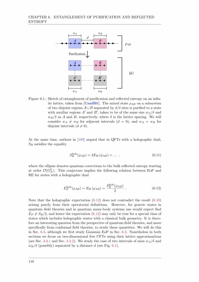
CHAPTER 6. ENTANGLEMENT OF PURIFICATION AND REFLECTEDENTROPY
wA wB
d
A B
Purification
A B
A B
AB
|
wA' wB'
Figure 6.1.: Sketch of entanglement of purification and reflected entropy on an infin-ite lattice, taken from [CamH01]. The mixed state AB on a subsystemof two disjoint regions A[B separated by d/ sites is purified to a statewith auxiliar regions A0 and B0, taken to be of the same size wA/ andwB/ as A and B, respectively, where is the lattice spacing. We willconsider wA 6= wB for adjacent intervals (d = 0), and wA = wB fordisjoint intervals (d 6= 0).
At the same time, authors in [169] argued that in QFTs with a holographic dual,SR satisfies the equality
SholoR (AB) = 2EW (AB) + . . . , (6.11)
where the ellipsis denotes quantum corrections to the bulk reflected entropy startingat order O(G0
N ). This conjecture implies the following relation between EoP andRE for states with a holographic dual
EholoP (AB) = EW (AB) =
SholoR (AB)
2. (6.12)
Note that the holographic expectation (6.12) does not contradict the result (6.10)arising purely from their operatorial definitions. However, for generic states inquantum field theories and in quantum many-body systems one would expect findEP 6= SR/2, and hence the expectation (6.12) may only be true for a special class ofstates which includes holographic states with a classical bulk geometry. It is there-fore an interesting question from the perspective of quantum field theories, and morespecifically from conformal field theories, to study these quantities. We will do thisin Sec. 6.3, although we first study Gaussian EoP in Sec. 6.2. Nonetheless in bothsections we focus on two-dimensional free CFTs using their lattice approximations(see Sec. 3.3.1 and Sec. 3.3.2). We study the case of two intervals of sizes wA/ andwB/ (possibly) separated by a distance d (see Fig. 6.1).
110
6.2. GAUSSIAN ENTANGLEMENT OF PURIFICATION
6.2. Gaussian Entanglement of Purification
Until very recently, most of the understanding of EoP came from its conjecturedholographic realization as the dual of the entanglement wedge cross-section (6.5),a series of results determined by local conformal transformations in CFTs and bystudies in free QFTs for subsystems with a small number of degrees of freedom.In this section, based on [CamH02], we go beyond the previously known results inthe latter case by computing EoP using the most general Gaussian purificationsof Gaussian mixed states corresponding to vacuum subregions of free bosonic andfermionic CFTs; that is, essentially using the same models that we used for CoP inSec. 5.2. This allows us to approach the QFT limit and uncover properties of EoPin this regime.
Starting from a Gaussian mixed state GAB, we consider a Gaussian purification| Gi 2 H0 = HAB HA0B0 and then perform minimization of the entanglemententropy of the reduced density matrix GAA0 = trBB0(| Gi h G|) over Gaussian states
of the form UG | Gi where UG = 1AB UGA0B0 is a Gaussian unitary. In other words,
we focus on Gaussian entanglement of purification
EGP (
GAB) := min
UG=1ABUGA0B0
hStrBB0
UG | Gi h G| (UG)†
i, (6.13)
which in general is expected to satisfy the inequality EP (GAB) EG
P (GAB). That
is, Gaussian EoP EGP (
GAB) bounds the true EoP EP (
GAB) from above. How-
ever, as mentioned in Sec. 5.1, there is numerical evidence [226] which supportsthe conjecture [304] that for Gaussian mixed states this is actually an equalityEP (
GAB) EG
P (GAB), meaning that Gaussian purifications of Gaussian mixed states
suffice to reach the true minimum over all possible purifications.
Similarly to CoP, we can rephrase this minimization in terms of the complex struc-ture of the Gaussian purification |Ji of the Gaussian mixed state AB. In thiscase, all the necessary information about the purified Gaussian state is encoded inthe complex structure J of the state, which can be decomposed similarly to (5.9)as
J =
JAB JABA0B0
JA0B0AB JA0B0
, (6.14)
and which is of dimension (NA[B + NA0[B0) (NA[B + NA0[B0). In this case, the(Gaussian) entanglement entropy SAA0(|Ji) can be direclty computed via
SAA0(|Ji) =(
trAA0
1A+i JAA0
2 log1A+i JAA0
2
, (bosons)
trAA0
1A+i JAA0
2 log1A+i JAA0
2
, (fermions) .
(6.15)
These analytical expressions for entanglement entropy of Gaussian states were firstderived in [296, 297] and rephrased in terms of linear complex structures in [299,311].
The procedure to compute Gaussian EoP is then straightforward: we start with amatrix representation of the complex structure JAB of the mixed Gaussian state
AB in a basis a =aA,
aB
which decomposes JAB to a matrix of the form (5.5).
111
CHAPTER 6. ENTANGLEMENT OF PURIFICATION AND REFLECTEDENTROPY
This basis can be found from the eigenvectors of JAB. With this, we construct astarting purification of the form (5.7), with Nnm the number of ancillary degrees offreedom beyond the minimal purification.
In the basis a =aA,
aB,
aA0 , aB0
, the complex structure of the purified state has
the block form (6.14), where the diagonal blocks are precisely the complex structuresrestricted to the mixed states AB and A0B0 . By varying the block JA0B0 and theoff-diagonal blocks in a compatible way, we have access different purifications of AB.As a consequence, the Gaussian manifold over which we perform the minimizationis parametrized by transformations MA0B0 which act solely on the reduced complexstructure JA0B and acting on the full complex structure via M = 1AB MA0B0 . Theminimization can then be iteratively performed by varying MA0B0 with the steepest-descent method developed in [226].
In the following section (Sec. 6.2.1) we discuss the numerical results obtained in[CamH02] for Gaussian EoP for adjacent intervals for the discretized (1 + 1) -dimensional Klein–Gordon and critical transverse Ising CFT models using minimalpurifications Nnm = 0. The reason being that there exists numerical evidence [226]which shows that the minimum of (6.4) is reached when choosing the numbers ofdegrees of freedom of the purifying systems A0 and B0 is equal to the respectivenumbers of degrees of freedom in the original subsystems A and B, i.e., NA0 = NA
and NB0 = NB.
6.2.1. Adjacent Intervals in Free Conformal Field Theories
The guiding principle for our analysis of Gaussian EoP for adjacent intervals comesfrom the holographic expectation, represented in terms of the holographic formula (6.6).In particular, studies such as [160] performed analytical computations of EoP basedon path-integral optimization (see [104]) for holographic CFTs. In this case, foradjacent subsystems A and B of a boundary CFT it was found that
EW (A : B) =c
6log
2wAwB
(wA + wB)
, (6.16)
where here c is the central charge of the boundary CFT, wA and wB are the lengthsof the spatial boundary intervals A and B and where is a UV-regulator.
Starting from an equivalent adjacent interval setting, we applied the steepest des-cent method to the covariance matrices (3.45) and (3.83) in order to compute theGaussian EoP using minimal purifications (Nnm = 0) according to (6.13) and wefound
EP (A : B) =
(16 log
2wAwB
(wA+wB)δ
, (bosons)
112 log
2wAwB
(wA+wB)δ
, (fermions) ,
(6.17)
where here is the lattice spacing which acts as a UV regulator. These results arerepresented in Fig. 6.2 together with numerical data obtained for (wA+wB)/ = 12sites in chains of N = 100(wA + wB)/ total sites. From Fig. 6.2 we see a closeagreement between the numerical results and the holographic expectation (6.16)
112
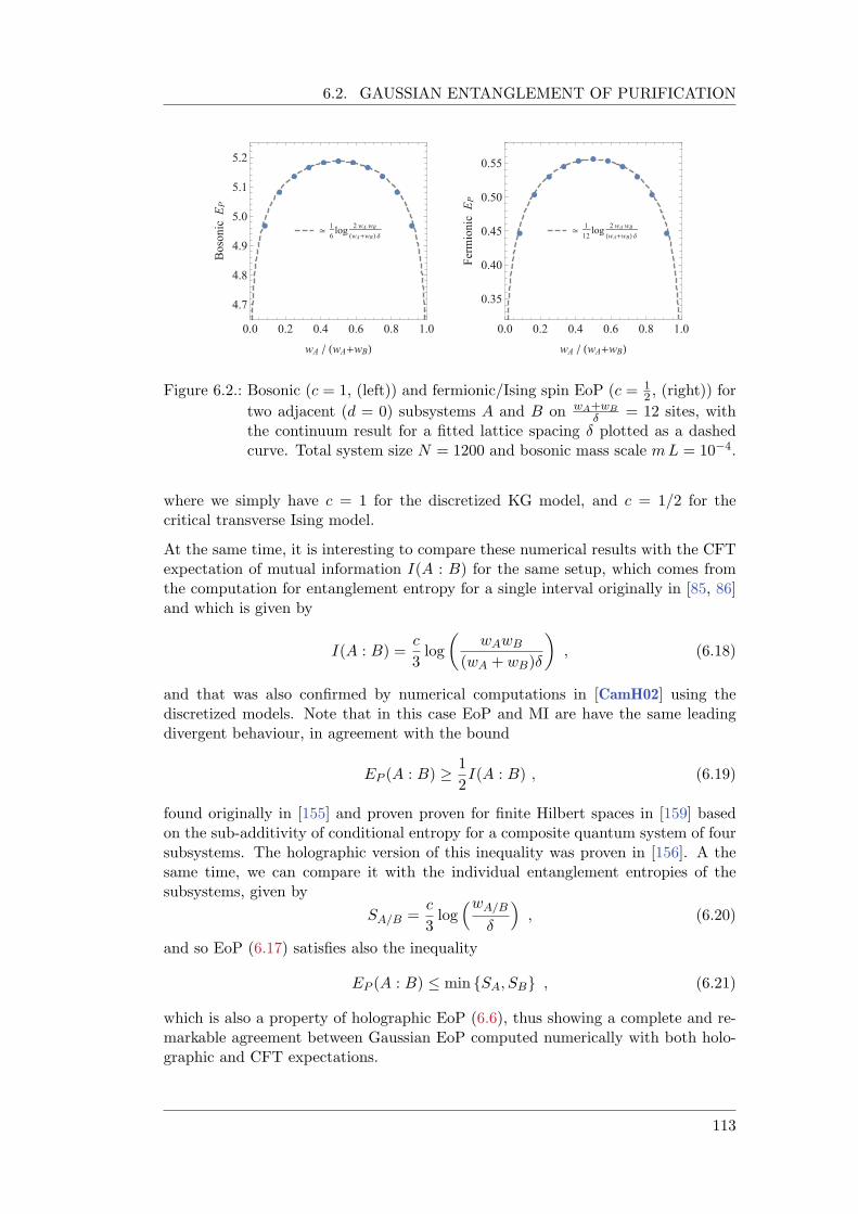
6.2. GAUSSIAN ENTANGLEMENT OF PURIFICATION
1
6log
2wA wB
(wA+wB)
0.0 0.2 0.4 0.6 0.8 1.0
4.7
4.8
4.9
5.0
5.1
5.2
wA / (wA+wB)
BosonicEP
1
12log
2wA wB
(wA+wB)
0.0 0.2 0.4 0.6 0.8 1.0
0.35
0.40
0.45
0.50
0.55
wA / (wA+wB)
FermionicEP
Figure 6.2.: Bosonic (c = 1, (left)) and fermionic/Ising spin EoP (c = 12 , (right)) for
two adjacent (d = 0) subsystems A and B on wA+wB
δ= 12 sites, with
the continuum result for a fitted lattice spacing plotted as a dashedcurve. Total system size N = 1200 and bosonic mass scale mL = 104.
where we simply have c = 1 for the discretized KG model, and c = 1/2 for thecritical transverse Ising model.
At the same time, it is interesting to compare these numerical results with the CFTexpectation of mutual information I(A : B) for the same setup, which comes fromthe computation for entanglement entropy for a single interval originally in [85, 86]and which is given by
I(A : B) =c
3log
wAwB
(wA + wB)
, (6.18)
and that was also confirmed by numerical computations in [CamH02] using thediscretized models. Note that in this case EoP and MI are have the same leadingdivergent behaviour, in agreement with the bound
EP (A : B) 1
2I(A : B) , (6.19)
found originally in [155] and proven proven for finite Hilbert spaces in [159] basedon the sub-additivity of conditional entropy for a composite quantum system of foursubsystems. The holographic version of this inequality was proven in [156]. A thesame time, we can compare it with the individual entanglement entropies of thesubsystems, given by
SA/B =c
3log
wA/B
, (6.20)
and so EoP (6.17) satisfies also the inequality
EP (A : B) min SA, SB , (6.21)
which is also a property of holographic EoP (6.6), thus showing a complete and re-markable agreement between Gaussian EoP computed numerically with both holo-graphic and CFT expectations.
113
CHAPTER 6. ENTANGLEMENT OF PURIFICATION AND REFLECTEDENTROPY
6.2.2. Small Separations in Free Bosonic CFTs
Here we investigate the behaviour Gaussian EoP for two disjoint intervals for thediscretized Klein–Gordon model in the small separation regime. We focus on thebosonic theory since the vacuum state of the critical transverse Ising CFT modelis generically non Gaussian for subsystems comprised of two disjoint intervals. Westudy EoP and RE for this model in the large separation limit in the followingsection, Sec. 6.3. At the same time, we focus on small separations for the bosonicmodel, since in this regime we can expect the zero-mode to be sub-dominant withrespect to the UV behaviour of EoP that we wish to extract. We comment on thebehaviour of bosonic EoP in the large separation limit also in Sec. 6.3.
We can use our Gaussian methods to study bosonic EoP for disjoint subsystems Aand B of sizes wA = wB = w in the small separation d regime, namely d w(see Fig. 6.1.). In this case, the holographic expectation [156, 157] and path-integraloptimization approach [160] predict a behaviour of EW (AB) of the form
EW (A : B)dw
=c
6log
2w
d
, (6.22)
which is consistent with (6.16) under the simple replacement = d and wA = wB =w.
Numerical results obtained with the steepest descent method for the discretizedKlein–Gordon model for a mass scale mL = 103 yield a logarithmic dependence ofbosonic Gaussian EoP in the d w regime given by
Ep(A : B)dw
1
6log
wd
1
2log(mL) + c0 , (6.23)
where c0 is a constant. Note that this result is consistent with the holographicexpectation (6.22) for c = 1.
At the same time, there exists the following universal result for mutual informationat small separations d w [86, 294]
I(A : B)dw
' c
3log
w
2d
, (6.24)
which is corroborated by numerical computations performed on the discretized modeland which yield the behaviour in the small d/w regime given by
I(A : B)num
dw a1 log
wd
1
2log(mL) + a0 . (6.25)
where a0 is a constant. The coefficient a1 can be bound according to 0.27 . a1 . 0.40by closely analysing the numerical behaviour of I(A : B) and S(A [ B) as donein [CamH02], suggesting an asymptotic behaviour a1 / 1/3 consistent with (6.24)for c = 1.
Note the logarithmicmL dependence present in both numerical results for EoP (6.23)and MI (6.25), which is a consequence of the fact that we are considering a massiveKG field model with small mass scale mL as a proxy for the modular invariant c = 1
114
6.2. GAUSSIAN ENTANGLEMENT OF PURIFICATION
bosonic CFT, as explained in Sec. 3.3.1. For MI this logarithmic divergence was firstobserved in [305].
We therefore also find in this case a remarkable agreement between the numericalresults for Gaussian EoP and the CFT and holographic expectations, which reliedon a benchmark set by an analysis of MI in this regime.
6.2.3. Large Separations in Free Bosonic CFTs
We now turn to the case of the large separation behaviour of bosonic GaussianEoP. In this case, numerical computations (see [CamH02]) show a behaviour akinto bosonic MI.3 This observation had already been made for smaller subsystemsand smaller separations in [305] and is consistent with the observation that EoPweighs classical and quantum correlations differently at mall distances, when bothbecome relevant. At large separations, both EoP and MI have a zero-mode contri-bution alongside a sub-polynomial (logarithmic or double-logarithmic) decay. Thatis, both MI and EoP suffer from an infrared divergence which can be regulated bya log(mL)/2 and log(log(mL))/2 term respectively. That is, bosonic EoP behavesin this limit as
EP (A : B)boswd
d1
wd
d2 1
2log(mL) + d0 , (6.26)
with d2 . 0.15 and d0 a constant, which is consistent with the absence of a long-distance power behavior. On the other hand, bosonic MI behaves as
I(A : B)boswd
' fMI
d
w
+
1
2log
log
1
m
, (6.27)
where two possibilities for a behaviour of the coefficient fMI explored in [CamH02]are given by
fMI (
g0 g1log
dw
g2,
h0 h1log
log
dw
h2,
(6.28)
with g2 . 0.1 and h2 . 1.3, showing the likelihood of a double-logarithmic decay ofbosonic MI in an infinite line set-up.
As opposed to (6.26), in (6.27) the numerical computations were performed on aninfinite line, i.e., taking the limit m ! 0 only after the limit N ! 1. Thisanalysis differs from the periodic set-up, which was used to find (6.26) and where weconsidered the limit of a large number of sites N with the mass scale mL = mNconstant and small. In this limit, the mass dependence of both MI and EoP isaccurately described by log(mL)/2. The sub-polynomial dependence (6.28) in theinfinite line (as well as in the periodic setup) for MI contradicts earlier numericalobservations of a power law [312].
3Recall that a free scalar field (~x) in D dimensions has a scaling dimension ∆ = (D2)/2, whichimplies that in D = 2 the scalar field operator transforms trivially ! under a scalingtransformation ~x ! ~x. Therefore, the formula (6.31) for MI and analysis of the previoussection do not apply to the discretized Klein–Gordon model in (1 + 1)-dimensions, which leadsto a gapless CFT at criticality m ! 0.
115
CHAPTER 6. ENTANGLEMENT OF PURIFICATION AND REFLECTEDENTROPY
6.2.4. Universal Behaviour of Reflected Entropy in 2-dimensional ConformalField Theories
So far we have discussed the behaviour of EoP in the context of free (1 + 1)-dimensional bosonic and fermionic CFTs. However, the behaviour of reflected en-tropy (RE) in CFTs has also been explored in [313–315].
In particular, authors in [313] find a universal behaviour of RE across 2-dimensionalCFTs corroborated by [314, 315]. Authors compute RE using replica techniquesaccording to [169] yielding an expression of RE determined by conformally invariantcross-ratios xA,B, which in the case of two intervals of sizes wA and wB separatedby a distance d take the form
xA,B =wAwB
(d+ wA)(d+ wB), (6.29)
in such a way that for adjacent intervals d = 0 RE has the universal form
SR(A : B) =c
3log
2wAwB
(wA + wB)
, (6.30)
where here is also a UV regulator. From here we can see that EoP and RE ofadjacent intervals follow closely the holographic expectation (6.12). We will see inthe following section, that generically this is not the case for disjoint intervals thatare separated from each other.
6.3. Long Distance Behaviour in Free Conformal Field Theories
In this final section of the Chapter, we present the study of EoP and RE for twospherical subregions far away from each other in the vacuum of a CFT in any dimen-sion, following [CamH01]. This simple yet revealing set-up will allow us to extractuniversal properties of EoP and RE across CFTs which do not rely on intrinsic prop-erties of the states in consideration, such as Gaussianity, or particular propertiesof the CFT. In particular, we will perform this analysis using quantum many-bodytechniques and elementary properties of EE without relying on conformal symmetry.We will first present the general arguments which we propose to hold in general forCFTs in any dimension with a gap in the operator spectrum and then provide aconcrete example with explicit computations using the (1 + 1)-dimensional c = 1/2Ising CFT in the language of spins and fermions.
The basic setting of interest consists of two spherical regions of equal diameter wseparated by a distance d. Fig. 6.1 displays this set-up in the case of a (1 + 1)-dimensional CFT where the spherical subregions correspond to intervals of size w.The starting point for our analysis is the behaviour of MI (6.2) in the large separationregime. Recall that MI is generically a non-universal quantity which is computedfrom the 4-point function of twist operators, which is spectrum dependent [86]. Atlarge separations between two subregions in a CFT, such that d/w 1, MI decaysas
I(A : B) ' NΓ(3/2)Γ(2∆+ 1)
24∆+1Γ(2∆+ 3/2) 2∆ + . . . , (6.31)
116
6.3. LONG DISTANCE BEHAVIOUR IN FREE CONFORMAL FIELDTHEORIES
where
∆ :=wd
2∆, (6.32)
and where ∆ corresponds to the scaling dimension of the lowest non-trivial oper-ator(s) in the theory [302, 303], N is a factor denoting the possible degeneracyof such operators and the ellipsis denotes additional terms with a faster decay in∆ [301, 303, 316]. Formula (6.31) applies to CFTs with a gap in the operatorspectrum with the lowest one(s) being scalar(s).
6.3.1. General Argument
Our goal in this section is to find and prove an analogous formula to (6.31) for EoPand RE assuming the existence of a gap in the operator spectrum of the CFT. ForRE there is in fact recent numerical evidence [314, 315] which shows that in freeCFTs
SR ' ↵2∆ log(2∆
) + . . . with ∆ 1 , (6.33)
where ↵ is a positive constant which depends on the particular theory. We willshow that this asymptotic form holds both for EoP and RE in CFTs with a gappedspectrum and which have a lattice realization.
The fundamental assumption that will be the basis for our analysis and which willbe valid both for EoP and RE is that the density matrix AB of spherical subregionsA and B which are largely separated from each other can be written in the followingway
AB(∆) ' (0)A (0)B + ∆
(1)AB +
1
2∆
(2)AB + · · · , (6.34)
where the ellipsis denotes terms with higher (non necessarily integer) powers of ∆.We also assume that this asymptotic behaviour of the reduced density matrix holdsfor any sizes of the Hilbert spaces associated with the spherical subregions A and B.Note that terms with negative powers of ∆ are not allowed as these would contradictthe known decay of correlations with the separation d between A and B.
It is important to note that the linear term in ∆ in (6.34) must be non-vanishingin order to have a power-law scaling of correlations functions which involve theinsertions of the operator with the lowest scaling dimension in A and B. We willnot assume anything in particular about the term which is quadratic in ∆, thoughwe will show that it does not contribute to the leading term in the large distancebehaviour of EoP and RE.
The asymptotic behaviour of the reduced density matrix (6.34) can be seen as aconsequence of the formal expression of a generic purification | iABA0B0 | i 2HABA0B0 with perturbative expansion
| i ' | (0)i+ ∆ | (1)i+ 1
22∆ | (2)i+ . . . , (6.35)
where the leading term | (0)i factorizes as
| (0)i | (0)AA0i |
(0)BB0i , (6.36)
117
CHAPTER 6. ENTANGLEMENT OF PURIFICATION AND REFLECTEDENTROPY
in order to be consistent with the decomposition of (0)AB =
(0)A
(0)B in (6.34).
Furthermore, both the purification | i (6.35) as well as the term responsible for theinfinite separation behaviour, namely, | (0)i, are normalized
h | i = 1 , (6.37a)
h (0)| (0)i = h (0)AA0 |
(0)AA0i h (0)
BB0 | (0)BB0i = 1 , (6.37b)
with h (0)AA0 |
(0)BB0i = 0. These normalization conditions, in turn, lead to the following
constraints for | (1)i and | (2)i
h (0)| (1)i+ h (1)| (0)i = 0 , (6.38a)
h (0)| (2)i+ 2 h (1)| (1)i+ h (2)| (0)i = 0 . (6.38b)
From the definitions of EoP and RE, (6.4) and (6.9) respectively, we see that theirlarge separation asymptotics is determined by the behaviour of the eigenvalues µjof the reduced density matrix
AA0 := trBB0(| i h |) , (6.39)
as these determine the EE
SAA0 := trAA0(AA0 log(AA0)) = X
j0
µj log(µj) . (6.40)
From here we can see that in the infinite separation limit ∆ ! 0 the fact that
AB(∆ ! 0) factorizes to (0)A
(0)B also implies that in this limit the reduced
density matrix AA0(∆ ! 0) describes a pure state and as a consequence has a singlenon-zero eigenvalue µ0 = 1, with µj>1 = 0. Of course, this behaviour is modified byconsidering a large but finite separation of the spherical subregions.
We can generically expect that the density matrix AA0 be well-defined regardlessof the sign of ∆ when viewed as a formal parameter. As a consequence the linearcorrection to µj0 proportional to ∆ can be expected to vanish and therefore thefirst possible correction to µj0 in the large distance expansion must be proportionalto 2
∆. In other words, we can expect the leading asymptotic behaviour of the
eigenvalues of AA0 to be given by
µ0 1 ↵tot2∆ , (6.41a)
µj>0 ↵j2∆ , (6.41b)
where
↵tot :=X
j>0
↵j . (6.42)
for ↵j>0 0. We stress that this is not necessarily the case for AA0 arising from ageneric CFT but that the form (6.41) indeed encapsulates the possible leading orderasymptotic behaviour. In particular, if ↵j = 0 for all j > 0, then the behaviour (6.41)would simply involve an expression in terms of k
∆for k > 2.
118

6.3. LONG DISTANCE BEHAVIOUR IN FREE CONFORMAL FIELDTHEORIES
Assuming that the eigenvalues µj0 of AA0(∆) indeed have the asymptotic beha-viour (6.41), we directly find the EE (6.43) for any purification | i with perturbativeexpansion (6.35) given by
SAA0 ' ↵tot2∆ log(2
∆) + 2∆ + . . . , (6.43)
where
:=X
j>0
↵j (1 log(↵j)) . (6.44)
where the ellipsis in (6.43) denotes terms with higher powers in 2∆. Of course, there
are additional constraints on the purification (6.35) arising from the definitions ofEoP and RE which will determine the precise form of the leading coefficient ↵tot andoffset , as we will show. However, as we can already see, the form of the EE (6.43)has the same leading order behaviour as the numerical fits obtained in [314, 315] forRE encapsulated by (6.33).
A general guiding principle that we will follow is the observation that SAA0 isbounded from below [169] by
SAA0(| i) 1
2IAB(AB) , (6.45)
regardless of the purification | i and the long distance asymptotics, as proven inEq. (6) of [159]. As a consequence, given the asymptotic behaviour of MI (6.31), thebound (6.45) implies that at long distances SAA0 cannot have a leading behaviourwhich scales with a higher power than 2
∆. This fact combined with the analysis of
the eigenvalues µj of AA0 predicting that the highest power-law factor is exactly2∆
implies that ↵tot must be greater than 0. The consequence of this is that theasymptotic behaviour (6.45) necessarily applies to both EoP and RE for any CFTwith an operator gap and with a lattice realization.
Furthermore, since ↵tot > 0 is defined by (6.42) this means that there must existat least one ↵j>0 > 0 which in turn implies that the term in (6.43) containing theoffset must generically appear in such an expression. We remark once again thatthis is consistent with the results reported in [314, 315] where such a term was alsopresent in RE.
While this general argument only proves that ↵tot must be greater than zero, we cannevertheless provide more details about the information of the purification | i (6.35)which determines ↵tot. Indeed, a straightforward way to compute ↵tot is by calcu-lating the trace of 2AA0 which is giving lo leading order by
trAA0(2AA0) ' 1 2↵tot2∆ + · · · . (6.46)
Considering the general form of the purification (6.35) and defining
| (i)AA0i =
1AA0 h (0)
BB0 || (i)i , (6.47a)
| (i)BB0i =
h (0)
AA0 | 1BB0
| (i)i , (6.47b)
119
CHAPTER 6. ENTANGLEMENT OF PURIFICATION AND REFLECTEDENTROPY
for i 2 0, 1, 2, we find that the reduced density matrix AA0 is in general givenby
AA0 = | (0)AA0i h (0)
AA0 |+ ∆
|
(0)AA0i h (1)
AA0 |+ | (1)AA0i h (0)
AA0 |+
+1
22∆
|
(2)AA0i h (0)
AA0 |+ 2trBB0
| (1)i h (1)|
+ |
(0)AA0i h (2)
AA0 |
,(6.48)
which allows us to directly compute tr(2AA0). By imposing the constraints (6.38)arising from the normalization conditions (6.37) we find that ↵tot is given by
↵tot = k| (1)ik2 + |h (0)| (1)i|2 k| (1)AA0ik2 k| (1)
BB0ik2 . (6.49)
As claimed in the paragraph below (6.34), from (6.49) we can see that indeed theterm proportional to 2
∆in AB given by (6.34) does not contribute to the leading
coefficient ↵tot. This insight has the potential to provide a way of fixing the the formof ↵tot for EoP and RE in terms of CFT data in an akin manner as to how (6.31)provides it for the computation of MI.
While for RE obtaining ↵tot involves a direct computation using the canonical puri-fication of the reduced density matrix AB, for EoP it amounts to solving a minim-ization problem of the quadratic polynomial (6.49) obtained from the componentsof | (1)i and subject to the constraint (6.37a) and additional condition
(1)AB = trA0B0
| (1)i h (0)|+ | (0)i h (1)|
, (6.50)
generally leading to constraints on | (1)i. We expect these expressions to have awell-defined minimum based on the arguments that we presented above. At thesame time, it is important to note that while ↵tot does not depend on 2AB, theindividual ↵j>0 do, and as a consequence so does the offset (6.44).
To provide a concrete realization of this analysis we will now consider on the criticalIsing model and the closely related fermionic CFT, which have also been the focus ofthe previous chapter on CoP. We will show how we can obtain the numerical valuesof the leading coefficient ↵tot and offset for EoP and RE and in particular comparewith the numerical results for RE appearing in [314, 315].
Consider the (1 + 1)-dimensional critical (J = Jz = 1) transverse Ising model on aninfinite line with Hamiltonian (3.66) given in terms of generalized Pauli operatorsSx,zi (see (3.68))
H = 1X
i=1
2Sx
i Sxi+1 + Sz
i
, (6.51)
which defines the c = 1/2 Ising CFT. In this case the non-degenerate (N = 1)lightest operator of scaling dimension ∆ = 1/8 corresponds to the spin operator Sx
i ,often called the spin field and denoted simply by .
The Ising model can be mapped to a free fermion theory in terms of Majorana modesusing the Jordan–Wigner transformation, as we did in Sec. 3.3.2. It is important tomention, however, that the set-up we are interested in, namely the reduced density
120
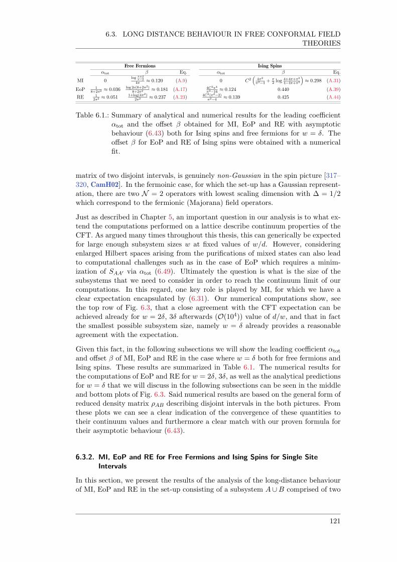
6.3. LONG DISTANCE BEHAVIOUR IN FREE CONFORMAL FIELDTHEORIES
Free Fermions Ising Spins
↵tot Eq. ↵tot Eq.
MI 0log π+2
π2
4π 0.120 (A.9) 0 C2
4π2
π24+ π
2 log4+4π+π2
44π+π2
0.298 (A.31)
EoP 18+2π2 0.036 log 2e(8+2π2)
8+2π2 0.181 (A.17) 4C2π4
π416 0.124 0.440 (A.39)
RE 12π2 0.051 1+log(4π2)
2π2 0.237 (A.23) 4C2(π22)π24
0.139 0.425 (A.44)
Table 6.1.: Summary of analytical and numerical results for the leading coefficient↵tot and the offset obtained for MI, EoP and RE with asymptoticbehaviour (6.43) both for Ising spins and free fermions for w = . Theoffset for EoP and RE of Ising spins were obtained with a numericalfit.
matrix of two disjoint intervals, is genuinely non-Gaussian in the spin picture [317–320, CamH02]. In the fermoinic case, for which the set-up has a Gaussian represent-ation, there are two N = 2 operators with lowest scaling dimension with ∆ = 1/2which correspond to the fermionic (Majorana) field operators.
Just as described in Chapter 5, an important question in our analysis is to what ex-tend the computations performed on a lattice describe continuum properties of theCFT. As argued many times throughout this thesis, this can generically be expectedfor large enough subsystem sizes w at fixed values of w/d. However, consideringenlarged Hilbert spaces arising from the purifications of mixed states can also leadto computational challenges such as in the case of EoP which requires a minim-ization of SAA0 via ↵tot (6.49). Ultimately the question is what is the size of thesubsystems that we need to consider in order to reach the continuum limit of ourcomputations. In this regard, one key role is played by MI, for which we have aclear expectation encapsulated by (6.31). Our numerical computations show, seethe top row of Fig. 6.3, that a close agreement with the CFT expectation can beachieved already for w = 2, 3 afterwards (O(104)) value of d/w, and that in factthe smallest possible subsystem size, namely w = already provides a reasonableagreement with the expectation.
Given this fact, in the following subsections we will show the leading coefficient ↵tot
and offset of MI, EoP and RE in the case where w = both for free fermions andIsing spins. These results are summarized in Table 6.1. The numerical results forthe computations of EoP and RE for w = 2, 3, as well as the analytical predictionsfor w = that we will discuss in the following subsections can be seen in the middleand bottom plots of Fig. 6.3. Said numerical results are based on the general form ofreduced density matrix AB describing disjoint intervals in the both pictures. Fromthese plots we can see a clear indication of the convergence of these quantities totheir continuum values and furthermore a clear match with our proven formula fortheir asymptotic behaviour (6.43).
6.3.2. MI, EoP and RE for Free Fermions and Ising Spins for Single SiteIntervals
In this section, we present the results of the analysis of the long-distance behaviourof MI, EoP and RE in the set-up consisting of a subsystem A[B comprised of two
121
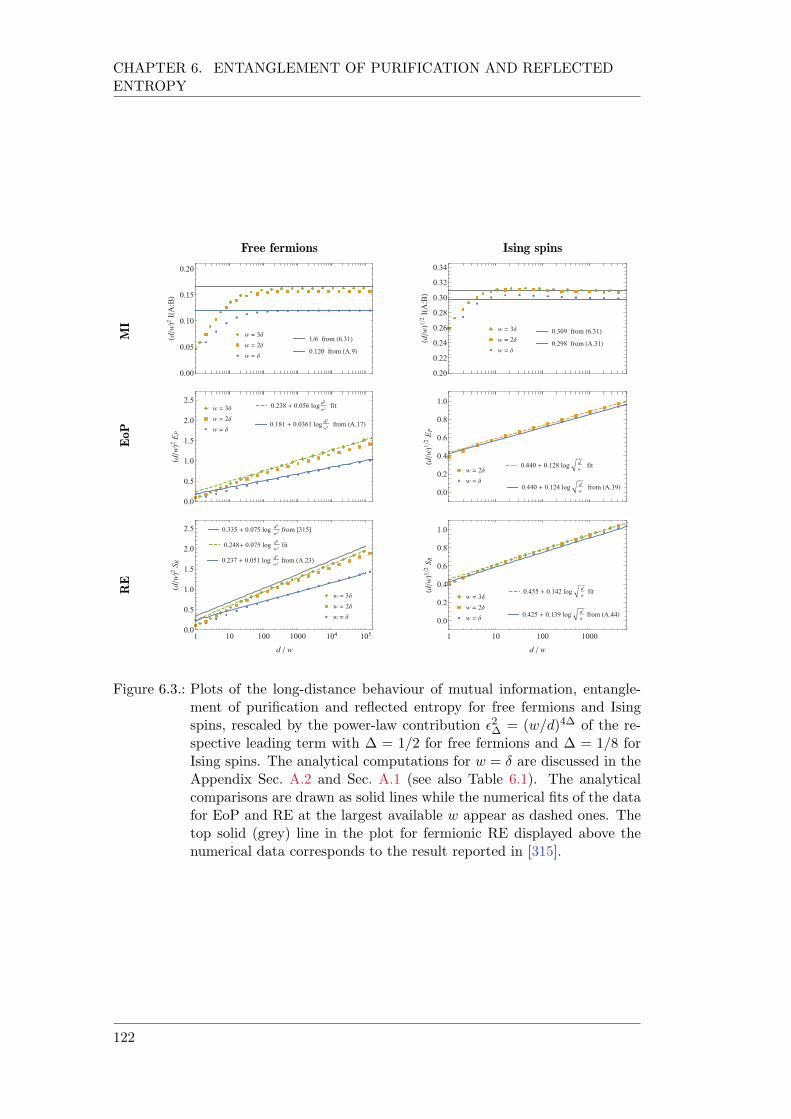
CHAPTER 6. ENTANGLEMENT OF PURIFICATION AND REFLECTEDENTROPY
Free fermions Ising spins
MI
1/6 from (6.31)
0.120 from (A.9)
w = 3
w = 2
w =
0.00
0.05
0.10
0.15
0.20
(d/w)2I(A:B)
0.309 from (6.31)
0.298 from (A.31)
w = 3
w = 2
w =
0.20
0.22
0.24
0.26
0.28
0.30
0.32
0.34
(d/w)12I(A:B)
EoP
w = 3
w = 2
w =0.181 + 0.0361 log
d2
w2from (A.17)
0.238 + 0.056 logd2
w2fit
0.0
0.5
1.0
1.5
2.0
2.5
(d/w)2EP
w = 2
w =0.440 + 0.124 log
d
wfrom (A.39)
0.440 + 0.128 logd
wfit
0.0
0.2
0.4
0.6
0.8
1.0
(d/w)12EP
RE
w = 3
w = 2
w =
0.335 + 0.075 logd2
w2from [315]
0.248+ 0.075 logd2
w2fit
0.237 + 0.051 logd2
w2from (A.23)
1 10 100 1000 104
105
0.0
0.5
1.0
1.5
2.0
2.5
d / w
(d/w)2SR
w = 3
w = 2
w =
0.455 + 0.142 logd
wfit
0.425 + 0.139 logd
wfrom (A.44)
1 10 100 1000
0.0
0.2
0.4
0.6
0.8
1.0
d / w
(d/w)12SR
Figure 6.3.: Plots of the long-distance behaviour of mutual information, entangle-ment of purification and reflected entropy for free fermions and Isingspins, rescaled by the power-law contribution 2
∆= (w/d)4∆ of the re-
spective leading term with ∆ = 1/2 for free fermions and ∆ = 1/8 forIsing spins. The analytical computations for w = are discussed in theAppendix Sec. A.2 and Sec. A.1 (see also Table 6.1). The analyticalcomparisons are drawn as solid lines while the numerical fits of the datafor EoP and RE at the largest available w appear as dashed ones. Thetop solid (grey) line in the plot for fermionic RE displayed above thenumerical data corresponds to the result reported in [315].
122
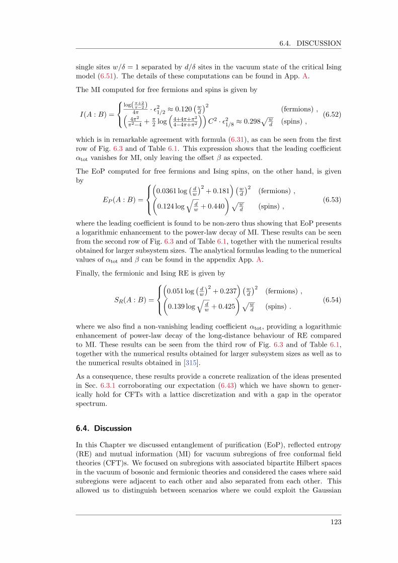
6.4. DISCUSSION
single sites w/ = 1 separated by d/ sites in the vacuum state of the critical Isingmodel (6.51). The details of these computations can be found in App. A.
The MI computed for free fermions and spins is given by
I(A : B) =
8<:
log(π+2π2)4π · 21/2 0.120
wd
2(fermions) ,
4π2
π24+ π
2 log4+4π+π2
44π+π2
C2 · 21/8 0.298
pwd (spins) ,
(6.52)
which is in remarkable agreement with formula (6.31), as can be seen from the firstrow of Fig. 6.3 and of Table 6.1. This expression shows that the leading coefficient↵tot vanishes for MI, only leaving the offset as expected.
The EoP computed for free fermions and Ising spins, on the other hand, is givenby
EP (A : B) =
8><>:
0.0361 log
dw
2+ 0.181
wd
2(fermions) ,
0.124 logq
dw + 0.440
pwd (spins) ,
(6.53)
where the leading coefficient is found to be non-zero thus showing that EoP presentsa logarithmic enhancement to the power-law decay of MI. These results can be seenfrom the second row of Fig. 6.3 and of Table 6.1, together with the numerical resultsobtained for larger subsystem sizes. The analytical formulas leading to the numericalvalues of ↵tot and can be found in the appendix App. A.
Finally, the fermionic and Ising RE is given by
SR(A : B) =
8><>:
0.051 log
dw
2+ 0.237
wd
2(fermions) ,
0.139 logq
dw + 0.425
pwd (spins) .
(6.54)
where we also find a non-vanishing leading coefficient ↵tot, providing a logarithmicenhancement of power-law decay of the long-distance behaviour of RE comparedto MI. These results can be seen from the third row of Fig. 6.3 and of Table 6.1,together with the numerical results obtained for larger subsystem sizes as well as tothe numerical results obtained in [315].
As a consequence, these results provide a concrete realization of the ideas presentedin Sec. 6.3.1 corroborating our expectation (6.43) which we have shown to gener-ically hold for CFTs with a lattice discretization and with a gap in the operatorspectrum.
6.4. Discussion
In this Chapter we discussed entanglement of purification (EoP), reflected entropy(RE) and mutual information (MI) for vacuum subregions of free conformal fieldtheories (CFT)s. We focused on subregions with associated bipartite Hilbert spacesin the vacuum of bosonic and fermionic theories and considered the cases where saidsubregions were adjacent to each other and also separated from each other. Thisallowed us to distinguish between scenarios where we could exploit the Gaussian
123
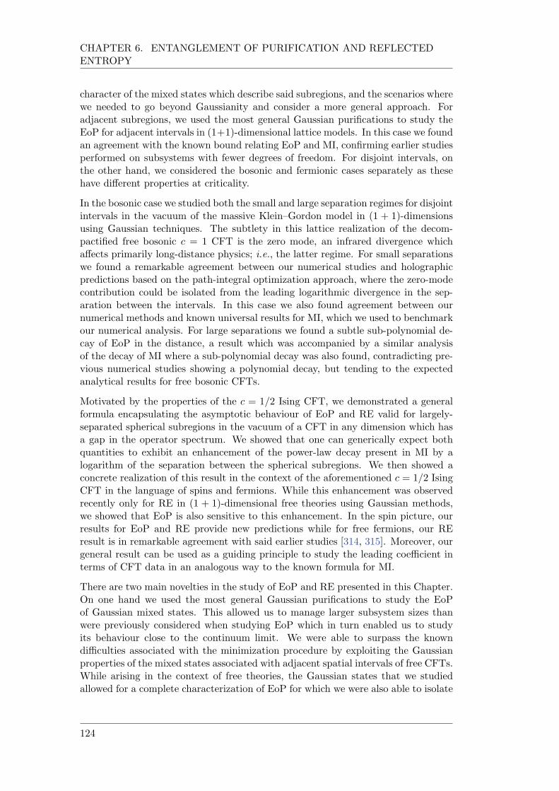
CHAPTER 6. ENTANGLEMENT OF PURIFICATION AND REFLECTEDENTROPY
character of the mixed states which describe said subregions, and the scenarios wherewe needed to go beyond Gaussianity and consider a more general approach. Foradjacent subregions, we used the most general Gaussian purifications to study theEoP for adjacent intervals in (1+1)-dimensional lattice models. In this case we foundan agreement with the known bound relating EoP and MI, confirming earlier studiesperformed on subsystems with fewer degrees of freedom. For disjoint intervals, onthe other hand, we considered the bosonic and fermionic cases separately as thesehave different properties at criticality.
In the bosonic case we studied both the small and large separation regimes for disjointintervals in the vacuum of the massive Klein–Gordon model in (1 + 1)-dimensionsusing Gaussian techniques. The subtlety in this lattice realization of the decom-pactified free bosonic c = 1 CFT is the zero mode, an infrared divergence whichaffects primarily long-distance physics; i.e., the latter regime. For small separationswe found a remarkable agreement between our numerical studies and holographicpredictions based on the path-integral optimization approach, where the zero-modecontribution could be isolated from the leading logarithmic divergence in the sep-aration between the intervals. In this case we also found agreement between ournumerical methods and known universal results for MI, which we used to benchmarkour numerical analysis. For large separations we found a subtle sub-polynomial de-cay of EoP in the distance, a result which was accompanied by a similar analysisof the decay of MI where a sub-polynomial decay was also found, contradicting pre-vious numerical studies showing a polynomial decay, but tending to the expectedanalytical results for free bosonic CFTs.
Motivated by the properties of the c = 1/2 Ising CFT, we demonstrated a generalformula encapsulating the asymptotic behaviour of EoP and RE valid for largely-separated spherical subregions in the vacuum of a CFT in any dimension which hasa gap in the operator spectrum. We showed that one can generically expect bothquantities to exhibit an enhancement of the power-law decay present in MI by alogarithm of the separation between the spherical subregions. We then showed aconcrete realization of this result in the context of the aforementioned c = 1/2 IsingCFT in the language of spins and fermions. While this enhancement was observedrecently only for RE in (1 + 1)-dimensional free theories using Gaussian methods,we showed that EoP is also sensitive to this enhancement. In the spin picture, ourresults for EoP and RE provide new predictions while for free fermions, our REresult is in remarkable agreement with said earlier studies [314, 315]. Moreover, ourgeneral result can be used as a guiding principle to study the leading coefficient interms of CFT data in an analogous way to the known formula for MI.
There are two main novelties in the study of EoP and RE presented in this Chapter.On one hand we used the most general Gaussian purifications to study the EoPof Gaussian mixed states. This allowed us to manage larger subsystem sizes thanwere previously considered when studying EoP which in turn enabled us to studyits behaviour close to the continuum limit. We were able to surpass the knowndifficulties associated with the minimization procedure by exploiting the Gaussianproperties of the mixed states associated with adjacent spatial intervals of free CFTs.While arising in the context of free theories, the Gaussian states that we studiedallowed for a complete characterization of EoP for which we were also able to isolate
124
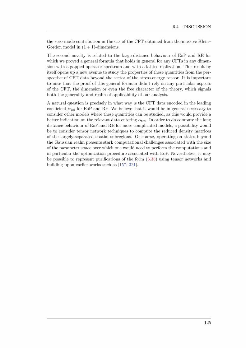
6.4. DISCUSSION
the zero-mode contribution in the cas of the CFT obtained from the massive Klein–Gordon model in (1 + 1)-dimensions.
The second novelty is related to the large-distance behaviour of EoP and RE forwhich we proved a general formula that holds in general for any CFTs in any dimen-sion with a gapped operator spectrum and with a lattice realization. This result byitself opens up a new avenue to study the properties of these quantities from the per-spective of CFT data beyond the sector of the stress-energy tensor. It is importantto note that the proof of this general formula didn’t rely on any particular aspectsof the CFT, the dimension or even the free character of the theory, which signalsboth the generality and realm of applicability of our analysis.
A natural question is precisely in what way is the CFT data encoded in the leadingcoefficient ↵tot for EoP and RE. We believe that it would be in general necessary toconsider other models where these quantities can be studied, as this would provide abetter indication on the relevant data entering ↵tot. In order to do compute the longdistance behaviour of EoP and RE for more complicated models, a possibility wouldbe to consider tensor network techniques to compute the reduced density matricesof the largely-separated spatial subregions. Of course, operating on states beyondthe Gaussian realm presents stark computational challenges associated with the sizeof the parameter space over which one would need to perform the computations andin particular the optimization procedure associated with EoP. Nevertheless, it maybe possible to represent purifications of the form (6.35) using tensor networks andbuilding upon earlier works such as [157, 321].
125
CHAPTER 6. ENTANGLEMENT OF PURIFICATION AND REFLECTEDENTROPY
126
7. Summary and Outlook
In this thesis we explored various aspects of complexity and entanglement for pureand mixed states in quantum field theory (QFT) inspired by the AdS/CFT cor-respondence. We focused primarily on three aspects of these quantities: the time-dependence of complexity in the context of non-equilibrium quantum dynamics real-ised through a solvable quantum quench model studied in detail in Chapter 4, theuniversal quantum information-theoretic properties of Gaussian mixed states en-capsulated by vacuum subregions of free CFTs and the long distance behaviour ofcorrelations in general bipartite subregions in any CFT with a gap in the operatorspectrum studied in Chapters 5 and 6.
Our study of non-equilibrium dynamics in Chap. 4 was based on a solvable quenchmodel through a critical point applied to a (1 + 1)-dimensional Klein–Gordon the-ory and was based on [CamH03]. Here we found that the complexity of the time-dependent ground state exhibits universal scalings which are dependent on the rateof the quantum quench t. In order to make our computations tractable, we con-sidered a lattice discretization of the theory which led us to consider the behaviour ofcomplexity in terms of the Fourier (momentum) mode decomposition of the groundstate. Then, by using the L2 norm of the circuit complexity constructed from unitarycircuits built from gates belonging to a closed subalgebra of the 2-dimensional sym-plectic algebra sp(2,R), we found that the full state complexity exhibits universalscalings as the theory goes through the critical point.
The Fuourier mode decomposition of the ground state allowed us to decompose thecomplexity of the full state in terms of the complexity of the individual momentummodes. We observed that both in the fast !0t 1 and slow Kibble–Zurek (KZ)!0t 1 regimes the zero-mode of the ground state dominates over higher mo-mentum modes and thus determines the overall scaling behaviour of complexity.The zero mode was found to have a logarithmic scaling in the slow regime and alinear one in the fast. The finding in the slow regime is particularly interestingsince it was also observed that entanglement entropy (EE) exhibits an equivalentscaling albeit with a different coefficient. In the case of a slow quantum quench, weshowed that the higher momentum modes saturate, a feature which prevents the fullcomplexity from exhibiting a clear scaling in this regime.
As we mentioned in Sec. 4.3, similar studies were carried out in the context ofthe relativistic fermionic Ising theory in [275]. In this case, a linear behaviour ofcomplexity was also observed in the sudden quench regime !0t ! 0, as well asa saturation of the higher modes in the slow quench regime t < (!0/4) csc
2(k/2).The main difference in this case is that the zero-mode contribution to the complexityvanishes. This is because the Bogoliubov transformation of the zero-mode which isused to determine the contribution is trivial, which is in turn due to the fact thatMajorana modes have independent zero-modes. Of course, in this case the zero-
127
CHAPTER 7. SUMMARY AND OUTLOOK
mode simply refers to the momentum mode with k = 0, and does not have anyassociated IR divergence as in the bosonic case.
Another difference between the work [275] and our results from Chapter 4 is that theformer evaluates complexity using the L1 norm assuming that the shortest circuitminimizes an L2 complexity. This is a commonly used technique to studying theformer case since the minimization of F1 cost functions are in general a challengingtask. Regardless of this, the analysis of the universal scalings fermionic complexitypresented in [275] presents strong similarities with the bosonic case. These workstherefore provide strong evidence that complexity, much like correlation functions orEE, is a useful quantity to study universal scalings in quantum quenches that takea theory through criticality.
A natural question which stems from this analysis is whether complexity is sensitiveto other kinds of phase transitions in quantum many-body systems out of equilib-rium. An example of an interesting question would be whether complexity is sensitiveto topological phase transitions. This has been studied recently in [322, 323] whereit was found that complexity can be used used to detect equilibrium and dynamicaltopological phase transitions by the presence of non-analyticity. An outstandingquestion is then whether complexity can be used for defining topological order. Cer-tain authors [324] claim that this is not the case, since complexity is an extensivequantity on the size of the system, and is thus inadequate for defining topologicalorder. It would be interesting to understand to what complexity can play a role inthe definition of topological order. A long-term goal would be to understand therole of complexity in more general models in condensed matter physics both in andout of equilibrium.
As we also mentioned previously, complexity has also entered the realm of cosmo-logy through the study of primordial perturbations [276]. It has also been used tostudy chaotic quantum systems [325–331]. It will be interesting to study whethercomplexity can bring new insights in other areas of physics. Whether it be in otherinteresting quantum many-body models, or to offer a new perspective on phenomenaseemingly unrelated to quantum information.
In the context of complexity of purification (CoP) discussed in Chapter 5 and basedon [CamH03, CamH02] we showed that our results obtained from Gaussian mixedstates corresponding to vacuum subregions of free CFTs (Sec. 5.2) are in remarkableagreement with holographic expectations (2.19). To be precise, we showed that theleading divergences of CoP obtained for a single and two adjacent intervals in thevacuum of Ising (c = 1/2) and bosonic (c = 1) CFTs match the divergences ofthe dual holographic computations carried out in AdS3. In the case of subregionsconsisting of two compontents, as is the case for the adjacent intervals, we showedthat mutual complexity is a appropriate quantity which disposes of the leadingdivergence both in the fermionic and bosonic case. We also showed how an effectivemethod for computing the Gaussian CoP based on the steepest-descent methodallows for an effective method which does not require any further assumptions andsimplifications about the purifications of the mixed Gaussian states.
We also showed in the case of a two-harmonic oscillator system how the notions ofpure state complexity, CoP and EE capture different information about the state
128
as encoded in its covariance matrix. The claim that complexity of the pure state issensitive to more information about the state than EE is not surprising, however itremains to be determined what is the connection between complexity of subregions,as captured e.g., by CoP, and EE. In order to determine this, it is likely that we wouldneed to go beyond states which are Gaussian and hence completely characterised bytheir 2-point functions.
This naturally leads to the question whether one goes beyond Gaussian states infree theories and beyond scenarios in CFTs governed by the stress tensor sector. Inthe former case it would be interesting to study cases where the Gaussian Ansatz ofthe quantum state in consideration, whether it be pure or mixed, does not apply asthis would be the case in interacting theories. In this regard there would be bothconceptual and computational challenges that one would need to overcome.
One of the main challenges would be how to properly choose a universal gate set ofunitaries with which one can construct the quantum circuit relating the (potentially)non-Gaussian reference and target states. For Hilbert spaces of a sufficiently smalldimension this may not be too difficult and one can imagine having a universal gateset from which certain unitaries can be constructed. However the main difficultywould arise when asking about the optimal circuit which takes the reference stateto the target state. Assuming that one would work using an F2 cost function (3.8b)the challenge here would be how to find the geodesic distance. Computationallyspeaking, this is the biggest challenge that one needs to overcome in order to definea notion of circuit complexity for non-Gaussian states.
An approach which could be useful in this case can be drawn from the work [332],where authors quantify the non-Gaussian character of a (bosonic) quantum stateby introducing a non-Gaussianity measure based on the Hilbert–Schmidt distancebetween the state under examination and a reference Gaussian state. It his worthnoting that this definition applies to mixed states. This construction has beenused to define a notion of non-Gaussianity in continuous-variable systems naturallyappearing in quantum information [333].
In the context of complexity, these ideas could perhaps be applied to constructa notion of complexity for non-Gaussian states. A general strategy would be thefollowing: We first choose pure non-Gaussian target state and a Gaussian referencestate . We then construct a mixed Gaussian “intermediate” state such that its1- and 2-point functions match the ones for . This is because a non-Gaussian purestate will always define a mixed Gaussian reference state. In other words, only apure Gaussian state has 1- and 2-point functions of a pure Gaussian state, whilenon-Gaussian states have 1- and 2-point functions that can only be matched to amixed Gaussian state. We then compute the Gaussian notion of complexity CG(,)between and using complexity of purification (5.4) or the Fisher–Rao distancefunction (5.45) as in [283]. We then construct the non-Gaussian complexity CnG(, )by using the Hilbert–Schmidt distance between and . Having computed bothcomplexities, we could need to compute the “total” complexity Ctot using a weightedsum of the individual complexities.
Conceptually, we would be solving the problem of defining non-Gaussian complex-ity by incorporating the standard Gaussian methods and a simple non-Gaussian
129
CHAPTER 7. SUMMARY AND OUTLOOK
method. This definition has furthermore have some desirable properties: If thenon-Gaussian target state is taken to be close to a Gaussian state, the previousdefinition will reduce to the usual Gaussian definition. More importantly, this mightbe a computable notion of non-Gaussian complexity. This notion, however, shouldperhaps be interpreted as a first order non-Gaussian approximation of a potentiallymore complicated definition of non-Gaussian complexity.
An example of a scenario were we could apply this ideas could be the case of twospins located in two separated sites in the vacuum of the critical Ising model con-sidered in Chapters 5 and 6 of this thesis. This set-up, as we thoroughly discussedin Sec. 6.3, is genuinely non-Gaussian and could potentially lead to a tractable im-plementation of these ideas. Essentially, the goal would be to arrive at a meaningfulnotion of complexity which we could use in interacting theories in order to bring thestudy of complexity in QFTs on similar footing to the status that EE has in theAdS/CFT correspondence: with well-defined computable notions on both sides ofthe holographic duality. Ultimately we would like to understand how exactly is theinformation about the interior of AdS black holes encoded in complexity.
Returning to the context of Gaussian states corresponding to vacuum subregions offree CFTs in (1+1)-dimensions, we performed analogous computations for entangle-ment of purification (EoP) based on [CamH02] where we were also able to find theleading divergent behaviour in agreement with holographic expectations obtainedwith the path-integral optimization method and with known bounds involving mu-tual information (MI) in for finite size Hilbert spaces in quantum information.
Of course, one can also wonder whether the computations that we have done forfree theories have some counterpart in a genuine string theory dual, based on theAdS/CFT correspondence. This is because following the discussion in the Intro-duction 1, one can also wonder if by taking the opposite limit which leads to thestrong/weak duality, i.e., the limit of small (1.7), one could arrive at a complement-ary weak/strong duality. That is, a strongly-interacting quantum gravity theory isdual to a weakly-coupled CFT. On this regard there are proposals in the contextof AdS4 holography [334], with a non-trivial test that triggered many developmentsin [335], and more recently in [336].
Insofar as the AdS/CFT correspondence provides a dynamical equivalence betweenthese theories for any values of the parameters which defines them it is to be expec-ted, at least in principle, that the free theory computations that we have discussedboth in the context of quantum quenches and of vacuum subregions of free CFTshave a counterpart at the level of the strongly-interacting string theory. This ofcourse, is an exceptionally difficult statement to prove, as string duals are notori-ously hard to work with.
Finally, in our study of the long-distance behaviour of EoP and reflected entropy(RE) presented in Sec. 6.3 and based on [CamH01] we proved a general formula whichapplies to any CFT with a gap in the operator spectrum and for any dimensions.The main assumption in this case being that the reduced density matrix defining theset-up of two spherical subregions of diameter w largely separated from each other(d/w 1) has a formal expansion in terms of the parameter ∆ = (w/d)2∆ aroundthe infinite separation limit, where we expect the state to be described by a product
130
state. Following these assumptions and assuming that the CFTs in question havea gap in the operator spectrum and a realization as lattice models, we prove thatEoP and RE have a logarithmic enhancement with respect to the known power-lawdecay of MI. This result opens the avenue for studying these quantities in a set-upwithin CFTs which is beyond the stress-energy tensor.
Understanding the way that the CFT data is encoded in these quantities can bridgethe gap between our understanding of their conjectured realizations in the AdS/CFTcorrespondence via the entanglement wedge cross-section, and their behaviour inCFTs. Given the relevance that the entanglement wedge has in the reconstructionof bulk regions associated with spatial boundary subregions, it is therefore necessaryto have a better understanding of these quantities from this perspective and ourresults set the stage for this enterprise.
In conclusion, the results that we discussed in this thesis set the stage for a betterunderstanding of complexity and entanglement in QFTs. This is paramount forelucidating the mechanism which connects gravity and quantum theories within theAdS/CFT correspondence. As a consequence, we believe that these can lead toa better understanding of quantum gravity and quite possible to new tools in thestudy of quantum many-body systems.
131
CHAPTER 7. SUMMARY AND OUTLOOK
132
A. Appendices
A. Long-Distance Behaviour of MI, EoP and RE
In this appendix we review the details of the computations of MI, EoP and RE inthe set-up consisting of a subsystem comprised of two single sites w/ = 1 in thevacuum state of the critical Ising model as discussed in Chap 6, Sec. 6.3.
A.1. Free Fermions
The starting point of our analysis of MI, EoP and RE is the set-up shown in Fig. A.1.
The first step for computing the MI involves the computation of the covariancematrix and reduced density matrix corresponding to the subsystem consisting of1 + 1 sites separated by d/w = d/ sites from the fermionic perspective, i.e., usingthe Majorana modes i (3.75). In this case ∆ = 1/2, ∆ = (w/d)2∆ correspondssimply to 1/2 = w/d. The fermionic covariance matrix is fully determined byrestricting the general expression of the infinite-size covariance matrix (3.86) to theaforementioned number of sites and is given by
ΩfermAB =
0BBB@
2π
2(2d/w+3)π
2π
2(2d/w+3)π
2(2d/w+3)π 2
π2
(2d/w+3)π2π
0
1CCCA . (A.1)
Note that the anti-diagonal terms in (A.1) can be rewritten in terms of 1/2 as21/2/(2+31/2). The reduced density matrix AB associated to this mixed statewith asymptotic behaviour (6.34) given by
fermAB ' (0)A
(0)B + 1/2
(1)AB + . . . , (A.2)
can be computed explicitly with respect to the basis ofHAB given by |##i , |"#i , |#"i ,|""i and is given by
fermAB '
0BB@
D 12π 1/2
EE
12π 1/2 F
1CCA , (A.3)
where
D =1
4+
1
+
1
2, E =
1
4 1
2, F =
1
4 1
+
1
2. (A.4)
133
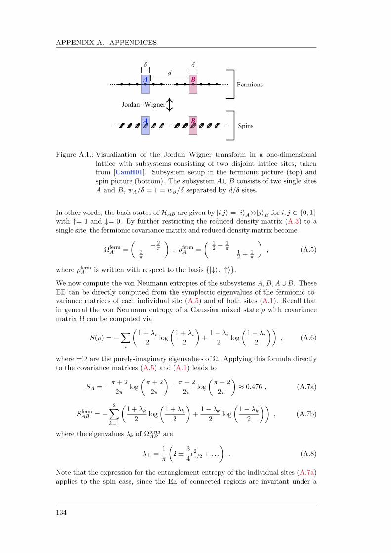
APPENDIX A. APPENDICES
d
A B
Jordan-Wigner
A B
Fermions
Spins
Figure A.1.: Visualization of the Jordan–Wigner transform in a one-dimensionallattice with subsystems consisting of two disjoint lattice sites, takenfrom [CamH01]. Subsystem setup in the fermionic picture (top) andspin picture (bottom). The subsystem A[B consists of two single sitesA and B, wA/ = 1 = wB/ separated by d/ sites.
In other words, the basis states of HAB are given by |i ji = |iiA|jiB for i, j 2 0, 1with "= 1 and #= 0. By further restricting the reduced density matrix (A.3) to asingle site, the fermionic covariance matrix and reduced density matrix become
ΩfermA =
2
π2π
, fermA =
12 1
π12 + 1
π
, (A.5)
where fermA is written with respect to the basis |#i , |"i.We now compute the von Neumann entropies of the subsystems A,B,A[B. TheseEE can be directly computed from the symplectic eigenvalues of the fermionic co-variance matrices of each individual site (A.5) and of both sites (A.1). Recall thatin general the von Neumann entropy of a Gaussian mixed state with covariancematrix Ω can be computed via
S() = X
i
1 + i
2log
1 + i
2
+
1 i2
log
1 i
2
, (A.6)
where ±i are the purely-imaginary eigenvalues of Ω. Applying this formula directlyto the covariance matrices (A.5) and (A.1) leads to
SA = + 2
2log
+ 2
2
2
2log
2
2
0.476 , (A.7a)
SfermAB =
2X
k=1
1 + k
2log
1 + k
2
+
1 k2
log
1 k
2
, (A.7b)
where the eigenvalues k of ΩfermAB are
± =1
2±
3
421/2 + . . .
. (A.8)
Note that the expression for the entanglement entropy of the individual sites (A.7a)applies to the spin case, since the EE of connected regions are invariant under a
134
A. LONG-DISTANCE BEHAVIOUR OF MI, EOP AND RE
Jordan–Wigner transformation. This implies a similar expansion for SAB (A.7b)which leads to a behaviour of the MI for w = given by
I ferm(A : B) 'log
π+2π2
421/2 + · · · ' 0.120
wd
2, (A.9)
which reproduces the correct power law of fermionic MI in the continuum limit, butwith a smaller coefficient than the continuum value (6.31). Note that this result alsomatches the long distance expansion of results known for Dirac fermions [337]
IDirac(A : B) =c
3log
(d+ w)2
d(2w + d)
=
1
621/2 =
1
6
wd
2, (A.10)
computed for two intervals of equal and arbitrary size w.
We use a similar perturbative expansion of the fermionic covariance matrix for twodisjoint intervals akin to (A.2) in terms of 1/2 in order to compute the fermionicEoP. For subsystems comprised of a single lattice site, the large separation expansionw = d of a purification of Ωferm
AB (A.1) is
Ω ' Ω(0) + 1/2Ω
(1) +1
221/2Ω
(2) + . . . , (A.11)
obtained in the limit 1/2 ! 0 and where
Ω(0) =
0BBBBBBBBBB@
G LG L
G LG L
L GL G
L GL G
1CCCCCCCCCCA
, (A.12)
is the purification of ΩAB in the infinite separation limit d/ ! 1 in the Hilbertspace HAB HA0B0 with G = 2/ and L =
p1G2.
By further imposing the constraint that Ω represents a pure sate Ω2 = 1 together
with constraints for Ω(1)AB and Ω
(2)AB arising from (6.38), one can find Ω
(0) and Ω(1) in
an iterative manner, first by solving Ω(1) in terms of Ω(0) and then Ω
(2) in terms ofΩ(0) and Ω
(1).
In order to determine the asymptotic behaviour of the symplectic eigenvalues iof ΩAA0 , we use the strategy mentioned in Sec. 6.3.1 which relies on computingtr(Ω2
AA0). In this case we have tr(Ω2AA0) = 2(21 + 22) and tr(Ω4
AA0) = 2(41 + 42),which allows us to obtain the asymptotic behaviour of the eigenvalues i given inthe limit 1/2 ! 0 by
1 = 2 1 ↵tot 21/2 , (A.13)
135
APPENDIX A. APPENDICES
where ↵tot depends on parameters found in Ω(1) and Ω
(2). With this computationwe directly find
↵tot =x14a23 x13x24 + 2
2+
G(x14 x23)1
2L
+(x14 x23)
2 + (x13 + x24)2
4L2,
(A.14)
where the parameters xij correspond to the unconstrained entries in the term Ω(1)
appearing in the expansion (A.11). In order to find the EoP, given by the theminimum of SAA0 , we need to minimize ↵tot over the xij . Given that (A.14) isquadratic in xij , its minimum value can be computed analytically leading to
↵tot =1
8 + 22 0.03605 . (A.15)
Similarly to MI, we can expand SAA0 P
i(log 2 λi
2 ) via the eigenvalues i up tosecond order in 1/2. In this way, we find both ↵tot the offset analytically leadingto
SAA0 ' 21/2↵tot log(
21/2) + ↵tot log
2e
↵tot
. (A.16)
Combining this expression with (A.15) yields the asymptotic behaviour of fermionicEoP given by
EfermP (A : B) '
1
8 + 22log(2
12
) +log 2e(8 + 22)
8 + 22
212
' 0.0361 log
d
w
2
+ 0.181
!wd
2,
(A.17)
which agrees with the expected behaviour (6.43).
On the other hand, in order to compute the fermionic RE, we need to construct thecanonical purification of (A.3) via
|pABi =
X
i
pei |eii |eii = | (0)i+ 1/2 | (1)i+ . . . , (A.18)
where AB |eii = ei |eii. Note that we can construct the canonical purification|pABi exactly for the given form of the initial reduced density matrix AB and
hence we do not need to phrase our computation of RE in terms of covariancematrices as in the case of MI and EoP.
The term | (1)i can be computed directly using (A.18), leading to
| (1)i = 12π (|4i+ |13i) , (A.19)
with the states |ii forming the basis of HABA0B0 ordered as |####i , |"###i , |#"##i, |""##i , . . . , |""""i. From the density matrix of the canonical purification :=|pABi h
pAB| we restrict ourselves to the subsystems AA0 given by the reduced
136
A. LONG-DISTANCE BEHAVIOUR OF MI, EOP AND RE
density matrix AA0 = trBB0() and which has the asymptotic behaviour AA0 =
(0)A
(0)A0 + 21/2
(2)AA0/2 explicitly given by
AA0 ' (0)AA0 +1
221/2
(2)AA0 =
0BB@
G1 H
J
J
H G1 2π
1CCA , (A.20)
where
G1 = + 2
221/2
42, H =
p2 4
2p2 421/2
4(2 4), J =
21/2
42. (A.21)
We follow the same strategy as for EoP and compute the trace of the square of (A.20)from which we obtain
↵tot =1
22 0.051 . (A.22)
This shows that the fermionic RE, SR(AB) = SAA0(), exhibits the following asymp-totic behaviour
SfermR (A : B) '
1
22log 2
1/2 +1 + log(42)
22
21/2
=
0.051 log
d
w
2
+ 0.237
!wd
2,
(A.23)
where the offset in (A.23) was computed from the eigenvalues of (A.20) accordingto (6.44).
A.2. Ising Spins
The reduced density matrix of the Ising vacuum subregion of two disjoint siteswritten in terms of spin operators spinAB is genuinely non-Gaussian. However, follow-ing [319] we can still use Gaussian techniques to deduce its asymptotic behaviourin the limit d/w ! 1, or equivalently 1/8 ! 0. In this case, the reduced densitymatrix in the spin picture written with respect to the basis |""i , |#"i , |"#i , |##iconsistent with an asymptotic behaviour
spinAB '
(0)A
(0)B + 1/8
(1)AB + . . . , (A.24)
is given by
spinAB '
0BB@
D C · 1/8E C · 1/8
C · 1/8 E
C · 1/8 F
1CCA (A.25)
with D,E, F given by (A.4). As mentioned previously, in this case the lowest lyingoperator corresponds to the spin field with scaling dimension ∆ = 1/8 and as such
137
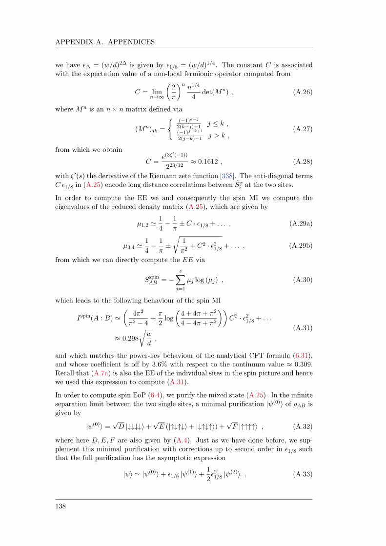
APPENDIX A. APPENDICES
we have ∆ = (w/d)2∆ is given by 1/8 = (w/d)1/4. The constant C is associatedwith the expectation value of a non-local fermionic operator computed from
C = limn!1
2
n n1/4
4det(Mn) , (A.26)
where Mn is an n n matrix defined via
(Mn)jk =
((1)kj
2(kj)+1 j k ,(1)jk+1
2(jk)1 j > k ,(A.27)
from which we obtain
C =e(3ζ
0(1))
223/12 0.1612 , (A.28)
with 0(s) the derivative of the Riemann zeta function [338]. The anti-diagonal termsC 1/8 in (A.25) encode long distance correlations between Sx
i at the two sites.
In order to compute the EE we and consequently the spin MI we compute theeigenvalues of the reduced density matrix (A.25), which are given by
µ1,2 '1
4 1
± C · 1/8 + . . . , (A.29a)
µ3,4 '1
4 1
±
r1
2+ C2 · 21/8 + . . . , (A.29b)
from which we can directly compute the EE via
SspinAB =
4X
j=1
µj log (µj) , (A.30)
which leads to the following behaviour of the spin MI
Ispin(A : B) '
42
2 4+
2log
4 + 4 + 2
4 4 + 2
C2 · 21/8 + . . .
0.298
rw
d,
(A.31)
and which matches the power-law behaviour of the analytical CFT formula (6.31),and whose coefficient is off by 3.6% with respect to the continuum value 0.309.Recall that (A.7a) is also the EE of the individual sites in the spin picture and hencewe used this expression to compute (A.31).
In order to compute spin EoP (6.4), we purify the mixed state (A.25). In the infiniteseparation limit between the two single sites, a minimal purification | (0)i of AB isgiven by
| (0)i =pD |####i+
pE (|"#"#i+ |#"#"i) +
pF |""""i , (A.32)
where here D,E, F are also given by (A.4). Just as we have done before, we sup-plement this minimal purification with corrections up to second order in 1/8 suchthat the full purification has the asymptotic expression
| i ' | (0)i+ 1/8 | (1)i+ 1
221/8 |
(2)i , (A.33)
138
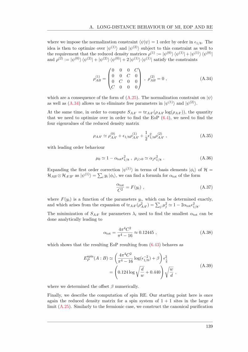
A. LONG-DISTANCE BEHAVIOUR OF MI, EOP AND RE
where we impose the normalization constraint h | i = 1 order by order in 1/8. The
idea is then to optimize over | (1)i and | (2)i subject to this constraint as well tothe requirement that the reduced density matrices (1) := | (0)i h (1)|+ | (1)i h (0)|and (2) := | (0)i h (2)|+ | (2)i h (0)|+ 2 | (1)i h (1)| satisfy the constraints
(1)AB =
0BB@
0 0 0 C0 0 C 00 C 0 0C 0 0 0
1CCA ,
(2)AB = 0 , (A.34)
which are a consequence of the form of (A.25). The normalization constraint on | ias well as (A.34) allows us to eliminate free parameters in | (1)i and | (2)i.
At the same time, in order to compute SAA0 = trAA0(AA0 log(AA0)), the quantitythat we need to optimize over in order to find the EoP (6.4), we need to find thefour eigenvalues of the reduced density matrix
AA0 ' (0)AA0 + 1/8(1)AA0 +
1
221/8
(2)AA0 , (A.35)
with leading order behaviour
µ0 ' 1 ↵tot21/8 , µj>0 ' ↵j
21/8 . (A.36)
Expanding the first order correction | (1)i in terms of basis elements |ii of H =HAB HA0B0 as | (1)i =
Pi yi |ii, we can find a formula for ↵tot of the form
↵tot
C2= F (yi) , (A.37)
where F (yi) is a function of the parameters yi, which can be determined exactly,and which arises from the expansion of trAA0(2AA0) =
Pj µ
2j ' 1 2↵tot
21/8.
The minimization of SAA0 for parameters i used to find the smallest ↵tot can bedone analytically leading to
↵tot =44C2
4 16 0.12445 , (A.38)
which shows that the resulting EoP resulting from (6.43) behaves as
EspinP (A : B) '
44C2
4 16log(2
1/8) +
218
=
0.124 log
rd
w+ 0.440
!rw
d,
(A.39)
where we determined the offset numerically.
Finally, we describe the computation of spin RE. Our starting point here is onceagain the reduced density matrix for a spin system of 1 + 1 sites in the large dlimit (A.25). Similarly to the fermionic case, we construct the canonical purification
139
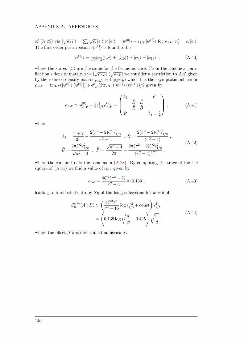
APPENDIX A. APPENDICES
of (A.25) via |pABi =
Pi
pei |eii |eii = | (0)i+ 1/8 |
(1)i for AB |eii = ei |eii.The first order perturbation | (1)i is found to be
| (1)i = πpπ24
(|7i+ |10i) + |4i+ |13i , (A.40)
where the states |ii are the same for the fermionic case. From the canonical puri-fication’s density matrix := |
pABi h
pAB| we consider a restriction to AA0 given
by the reduced density matrix AA0 = trBB0() which has the asymptotic behaviourAA0 = trBB0(| (0)i h (0)|) + 21/8(2trBB0(| (1)i h (1)|))/2 given by
AA0 ' (0)AA0 +12
21/8
(2)AA0 =
0BB@
A1 F
B E
E B
F A1 2π
1CCA , (A.41)
where
A1 = + 2
2
2(2 2)C221/8
2 4, B =
2(2 2)C221/8
(2 4),
E =2C221/8p2 4
, F =
p2 4
2
2(2 2)C221/8
(2 4)3/2,
(A.42)
where the constant C is the same as in (A.28). By computing the trace of the thesquare of (A.41) we find a value of ↵tot given by
↵tot =4C2(2 2)
2 4 0.139 , (A.43)
leading to a reflected entropy SR of the Ising subsystem for w = of
SspinR (A : B) '
4C24
4 16log 2
1/8 + const
21/8
=
0.139 log
rd
w+ 0.425
!rw
d,
(A.44)
where the offset was determined numerically.
140
Bibliography
[1] G. Aad et al., “Observation of a new particle in the search for the StandardModel Higgs boson with the ATLAS detector at the LHC,” Phys. Lett. B,vol. 716, pp. 1–29, 2012.
[2] S. Chatrchyan et al., “Observation of a New Boson at a Mass of 125 GeV withthe CMS Experiment at the LHC,” Phys. Lett. B, vol. 716, pp. 30–61, 2012.
[3] F. Englert and R. Brout, “Broken Symmetry and the Mass of Gauge VectorMesons,” Phys. Rev. Lett., vol. 13, pp. 321–323, 1964.
[4] P. W. Higgs, “Broken symmetries, massless particles and gauge fields,” Phys.Lett., vol. 12, pp. 132–133, 1964.
[5] B. P. Abbott et al., “Observation of Gravitational Waves from a Binary BlackHole Merger,” Phys. Rev. Lett., vol. 116, no. 6, p. 061102, 2016.
[6] B. P. Abbott et al., “Astrophysical Implications of the Binary Black-Hole Mer-ger GW150914,”Astrophys. J. Lett., vol. 818, no. 2, p. L22, 2016.
[7] A. Einstein, “Uber gravitationswellen,”Sitzungsberichte der Koniglich Preußis-chen Akademie der Wissenschaften (Berlin), pp. 154–167, 1918.
[8] K. Akiyama et al., “First M87 Event Horizon Telescope Results. I. The Shadowof the Supermassive Black Hole,”Astrophys. J. Lett., vol. 875, p. L1, 2019.
[9] M. Srednicki, Quantum field theory. Cambridge University Press, 1 2007.
[10] M. D. Schwartz, Quantum Field Theory and the Standard Model. CambridgeUniversity Press, 3 2014.
[11] S. W. Hawking and G. F. R. Ellis, The Large Scale Structure of Space-Time. Cambridge Monographs on Mathematical Physics, Cambridge Uni-versity Press, 2 2011.
[12] C. W. Misner, K. S. Thorne, and J. A. Wheeler, Gravitation. San Francisco:W. H. Freeman, 1973.
[13] R. M. Wald, General Relativity. Chicago, USA: Chicago Univ. Pr., 1984.
[14] J. D. Bekenstein, “Black holes and the second law,” Lett. Nuovo Cim., vol. 4,pp. 737–740, 1972.
[15] J. M. Bardeen, B. Carter, and S. W. Hawking, “The Four laws of black holemechanics,”Commun. Math. Phys., vol. 31, pp. 161–170, 1973.
[16] S. W. Hawking, “Black hole explosions?,”Nature, vol. 248, pp. 30–31, 1974.
[17] S. W. Hawking, “Particle Creation by Black Holes,” Commun. Math. Phys.,vol. 43, pp. 199–220, 1975. [Erratum: Commun.Math.Phys. 46, 206 (1976)].
141
Bibliography
[18] G. Penington, “Entanglement Wedge Reconstruction and the InformationParadox,” JHEP, vol. 09, p. 002, 2020.
[19] A. Almheiri, N. Engelhardt, D. Marolf, and H. Maxfield, “The entropy of bulkquantum fields and the entanglement wedge of an evaporating black hole,”JHEP, vol. 12, p. 063, 2019.
[20] D. N. Page, “Information in black hole radiation,” Phys. Rev. Lett., vol. 71,pp. 3743–3746, 1993.
[21] D. N. Page, “Time Dependence of Hawking Radiation Entropy,”JCAP, vol. 09,p. 028, 2013.
[22] A. Almheiri, T. Hartman, J. Maldacena, E. Shaghoulian, and A. Tajdini, “Theentropy of Hawking radiation,” arXiv:2006.06872 [hep-th], 6 2020.
[23] N. D. Birrell and P. C. W. Davies, Quantum Fields in Curved Space. Cam-bridge Monographs on Mathematical Physics, Cambridge, UK: CambridgeUniv. Press, 2 1984.
[24] R. M. Wald, Quantum Field Theory in Curved Space-Time and Black HoleThermodynamics. Chicago Lectures in Physics, Chicago, IL: University ofChicago Press, 1995.
[25] A. Almheiri, D. Marolf, J. Polchinski, and J. Sully, “Black Holes: Comple-mentarity or Firewalls?,” JHEP, vol. 02, p. 062, 2013.
[26] A. Y. Kitaev, A. H. Shen, and M. N. Vyalyi, Classical and Quantum Com-putation. Graduate Studies in Mathematics, American Mathematical Society,2006.
[27] I. Bengtsson and K. Zyczkowski, Geometry of Quantum States: An Introduc-tion to Quantum Entanglement. Cambridge University Press, 2006.
[28] M. A. Nielsen and I. L. Chuang, Quantum Computation and Quantum Inform-ation: 10th Anniversary Edition. Cambridge University Press, 2010.
[29] O. Aharony, S. S. Gubser, J. M. Maldacena, H. Ooguri, and Y. Oz, “Large Nfield theories, string theory and gravity,” Phys. Rept., vol. 323, pp. 183–386,2000.
[30] J. McGreevy, “Holographic duality with a view toward many-body physics,”Adv. High Energy Phys., vol. 2010, p. 723105, 2010.
[31] M. Ammon and J. Erdmenger, Gauge/gravity duality: Foundations and ap-plications. Cambridge: Cambridge University Press, 4 2015.
[32] D. Lust and S. Theisen, Lectures on string theory, vol. 346 of Lecture Notes inPhysics. Springer-Verlag Berlin Heidelberg, 1989.
[33] J. Polchinski, String theory. Vol. 1: An introduction to the bosonic string.Cambridge Monographs on Mathematical Physics, Cambridge UniversityPress, 12 2007.
142
Bibliography
[34] J. Polchinski, String theory. Vol. 2: Superstring theory and beyond. CambridgeMonographs on Mathematical Physics, Cambridge University Press, 12 2007.
[35] M. B. Green, J. H. Schwarz, and E. Witten, Superstring Theory Vol. 1: 25thAnniversary Edition. Cambridge Monographs on Mathematical Physics, Cam-bridge University Press, 11 2012.
[36] M. B. Green, J. H. Schwarz, and E. Witten, Superstring Theory Vol. 2: 25thAnniversary Edition. Cambridge Monographs on Mathematical Physics, Cam-bridge University Press, 11 2012.
[37] R. Blumenhagen, D. Lust, and S. Theisen, Basic concepts of string theory.Theoretical and Mathematical Physics, Heidelberg, Germany: Springer, 2013.
[38] J. M. Maldacena, “The Large N limit of superconformal field theories andsupergravity,” Int. J. Theor. Phys., vol. 38, pp. 1113–1133, 1999.
[39] G. ’t Hooft, “Dimensional reduction in quantum gravity,” Conf. Proc. C,vol. 930308, pp. 284–296, 1993.
[40] L. Susskind, “The World as a hologram,” J. Math. Phys., vol. 36, pp. 6377–6396, 1995.
[41] R. Bousso, “The Holographic principle,”Rev. Mod. Phys., vol. 74, pp. 825–874,2002.
[42] J. D. Bekenstein, “Black holes and entropy,” Phys. Rev. D, vol. 7, pp. 2333–2346, 1973.
[43] J. D. Bekenstein, “Generalized second law of thermodynamics in black holephysics,” Phys. Rev. D, vol. 9, pp. 3292–3300, 1974.
[44] J. D. Bekenstein, “A Universal Upper Bound on the Entropy to Energy Ratiofor Bounded Systems,” Phys. Rev. D, vol. 23, p. 287, 1981.
[45] H. Casini, “Relative entropy and the Bekenstein bound,”Class. Quant. Grav.,vol. 25, p. 205021, 2008.
[46] R. Bousso, “A Covariant entropy conjecture,” JHEP, vol. 07, p. 004, 1999.
[47] G. ’t Hooft, “A Planar Diagram Theory for Strong Interactions,”Nucl. Phys.B, vol. 72, p. 461, 1974.
[48] G. Policastro, D. T. Son, and A. O. Starinets, “The Shear viscosity of stronglycoupled N=4 supersymmetric Yang-Mills plasma,” Phys. Rev. Lett., vol. 87,p. 081601, 2001.
[49] P. Kovtun, D. T. Son, and A. O. Starinets, “Viscosity in strongly interactingquantum field theories from black hole physics,” Phys. Rev. Lett., vol. 94,p. 111601, 2005.
[50] J. D. Brown and M. Henneaux, “Central Charges in the Canonical Realizationof Asymptotic Symmetries: An Example from Three-Dimensional Gravity,”Commun. Math. Phys., vol. 104, pp. 207–226, 1986.
143
Bibliography
[51] S. S. Gubser, I. R. Klebanov, and A. M. Polyakov, “Gauge theory correlatorsfrom noncritical string theory,” Phys. Lett. B, vol. 428, pp. 105–114, 1998.
[52] E. Witten, “Anti-de Sitter space and holography,” Adv. Theor. Math. Phys.,vol. 2, pp. 253–291, 1998.
[53] T. De Jonckheere, “Modave lectures on bulk reconstruction in AdS/CFT,”PoS, vol. Modave2017, p. 005, 2018.
[54] D. Harlow, “TASI Lectures on the Emergence of Bulk Physics in AdS/CFT,”PoS, vol. TASI2017, p. 002, 2018.
[55] N. Beisert et al., “Review of AdS/CFT Integrability: An Overview,” Lett.Math. Phys., vol. 99, pp. 3–32, 2012.
[56] D. Serban, “Integrability and the AdS/CFT correspondence,” J. Phys. A,vol. 44, p. 124001, 2011.
[57] A. Sfondrini, “Towards integrability for AdS3/CFT2,” J. Phys. A, vol. 48,no. 2, p. 023001, 2015.
[58] S. A. Hartnoll, “Lectures on holographic methods for condensed matter phys-ics,”Class. Quant. Grav., vol. 26, p. 224002, 2009.
[59] J. Zaanen, Y.-W. Sun, Y. Liu, and K. Schalm, Holographic Duality in Con-densed Matter Physics. Cambridge Univ. Press, 2015.
[60] S. A. Hartnoll, A. Lucas, and S. Sachdev, Holographic quantum matter. TheMIT Press, 12 2016.
[61] J. Casalderrey-Solana, H. Liu, D. Mateos, K. Rajagopal, and U. A.Wiedemann, Gauge/String Duality, Hot QCD and Heavy Ion Collisions. Cam-bridge University Press, 2014.
[62] N. Brambilla et al., “QCD and Strongly Coupled Gauge Theories: Challengesand Perspectives,” Eur. Phys. J. C, vol. 74, no. 10, p. 2981, 2014.
[63] M. Baggioli, Applied Holography: A Practical Mini-Course. SpringerBriefs inPhysics, Springer, 2019.
[64] S. J. Devitt, W. J. Munro, and K. Nemoto, “Quantum error correction forbeginners,”Reports on Progress in Physics, vol. 76, p. 076001, Jun 2013.
[65] B. M. Terhal, “Quantum error correction for quantum memories,” Reviews ofModern Physics, vol. 87, p. 307–346, Apr 2015.
[66] R. Orus, “Tensor networks for complex quantum systems,”APS Physics, vol. 1,pp. 538–550, 2019.
[67] A. Jahn and J. Eisert, “Holographic tensor network models and quantum errorcorrection: A topical review,” arXiv:2102.02619 [quant-ph], 2 2021.
[68] R. Penrose, “Applications of negative dimensional tensors,” in Combinatorialmathematics and its applications (D. J. A. Welsh, ed.), Proceedings of a Con-ference held at the Mathematical Institute, Oxford, from 7-10 July, (London-New York), Academic Press, 1971.
144
Bibliography
[69] R. Penrose, “Angular momentum: an approach to combinatorial space-time,”in Quantum Theory and Beyond (T. Bastin, ed.), (Cambridge), pp. 151–180,Cambridge University Press, 1971.
[70] C. Rovelli and L. Smolin, “Spin networks and quantum gravity,” Phys. Rev.D, vol. 52, pp. 5743–5759, 1995.
[71] C. Rovelli, “Loop quantum gravity,” Living Rev. Rel., vol. 1, p. 1, 1998.
[72] S. R. White, “Density matrix formulation for quantum renormalizationgroups,” Phys. Rev. Lett., vol. 69, pp. 2863–2866, 1992.
[73] S. R. White, “Density-matrix algorithms for quantum renormalization groups,”Phys. Rev. B, vol. 48, pp. 10345–10356, 1993.
[74] S. Ostlund and S. Rommer, “Thermodynamic limit of density matrix renor-malization,” Physical Review Letters, vol. 75, p. 3537–3540, Nov 1995.
[75] J. Dukelsky, M. A. Martın-Delgado, T. Nishino, and G. Sierra, “Equivalence ofthe variational matrix product method and the density matrix renormalizationgroup applied to spin chains,”Europhysics Letters (EPL), vol. 43, p. 457–462,Aug 1998.
[76] M. B. Hastings, “An area law for one-dimensional quantum systems,” J. Stat.Mech., vol. 0708, p. P08024, 2007.
[77] F. Verstraete and J. I. Cirac, “Matrix product states represent ground statesfaithfully,” Physical Review B, vol. 73, Mar 2006.
[78] D. Perez-Garcia, F. Verstraete, M. M. Wolf, and J. I. Cirac, “Matrix ProductState Representations,” arXiv e-prints, pp. quant–ph/0608197, Aug. 2006.
[79] A. Weichselbaum, F. Verstraete, U. Schollwock, J. I. Cirac, and J. von Delft,“Variational matrix-product-state approach to quantum impurity models,”Physical Review B, vol. 80, Oct 2009.
[80] M. B. Hastings and T. Koma, “Spectral gap and exponential decay of correl-ations,”Commun. Math. Phys., vol. 265, pp. 781–804, 2006.
[81] M. Cramer, J. Eisert, M. B. Plenio, and J. Dreissig, “An Entanglement-arealaw for general bosonic harmonic lattice systems,” Phys. Rev. A, vol. 73,p. 012309, 2006.
[82] M. Srednicki, “Chaos and quantum thermalization,”Physical Review E, vol. 50,p. 888–901, Aug 1994.
[83] J. Eisert, M. Cramer, and M. B. Plenio, “Area laws for the entanglemententropy - a review,”Rev. Mod. Phys., vol. 82, pp. 277–306, 2010.
[84] J. L. Cardy and I. Peschel, “Finite Size Dependence of the Free Energy in Two-dimensional Critical Systems,”Nucl. Phys. B, vol. 300, pp. 377–392, 1988.
[85] C. Holzhey, F. Larsen, and F. Wilczek, “Geometric and renormalized entropyin conformal field theory,”Nucl. Phys. B, vol. 424, pp. 443–467, 1994.
145
Bibliography
[86] P. Calabrese and J. L. Cardy, “Entanglement entropy and quantum field the-ory,” J. Stat. Mech., vol. 0406, p. P06002, 2004.
[87] G. Vidal, “Entanglement Renormalization,” Phys. Rev. Lett., vol. 99, no. 22,p. 220405, 2007.
[88] G. Vidal, “Class of Quantum Many-Body States That Can Be Efficiently Sim-ulated,” Phys. Rev. Lett., vol. 101, p. 110501, 2008.
[89] B. Swingle, “Entanglement Renormalization and Holography,” Phys. Rev. D,vol. 86, p. 065007, 2012.
[90] N. Bao, C. Cao, S. M. Carroll, A. Chatwin-Davies, N. Hunter-Jones, J. Pollack,and G. N. Remmen, “Consistency conditions for an AdS multiscale entangle-ment renormalization ansatz correspondence,” Phys. Rev. D, vol. 91, no. 12,p. 125036, 2015.
[91] A. Milsted and G. Vidal, “Geometric interpretation of the multi-scale entan-glement renormalization ansatz,” arXiv:1812.00529 [hep-th], 2018.
[92] C. Beny, “Causal structure of the entanglement renormalization ansatz,”NewJ. Phys., vol. 15, p. 023020, 2013.
[93] B. Czech, L. Lamprou, S. McCandlish, and J. Sully, “Tensor Networks fromKinematic Space,” JHEP, vol. 07, p. 100, 2016.
[94] F. Pastawski, B. Yoshida, D. Harlow, and J. Preskill, “Holographic quantumerror-correcting codes: Toy models for the bulk/boundary correspondence,”JHEP, vol. 06, p. 149, 2015.
[95] J. Haegeman, T. J. Osborne, H. Verschelde, and F. Verstraete, “EntanglementRenormalization for Quantum Fields in Real Space,”Phys. Rev. Lett., vol. 110,no. 10, p. 100402, 2013.
[96] F. Verstraete and J. I. Cirac, “Continuous Matrix Product States for QuantumFields,” Phys. Rev. Lett., vol. 104, p. 190405, 2010.
[97] M. Nozaki, S. Ryu, and T. Takayanagi, “Holographic Geometry of Entangle-ment Renormalization in Quantum Field Theories,” JHEP, vol. 10, p. 193,2012.
[98] A. Mollabashi, M. Nozaki, S. Ryu, and T. Takayanagi, “Holographic Geometryof cMERA for Quantum Quenches and Finite Temperature,” JHEP, vol. 03,p. 098, 2014.
[99] J. S. Cotler, M. Reza Mohammadi Mozaffar, A. Mollabashi, and A. Naseh,“Entanglement renormalization for weakly interacting fields,” Phys. Rev. D,vol. 99, no. 8, p. 085005, 2019.
[100] J. Cotler, M. R. Mohammadi Mozaffar, A. Mollabashi, and A. Naseh, “Renor-malization Group Circuits for Weakly Interacting Continuum Field Theories,”Fortsch. Phys., vol. 67, no. 10, p. 1900038, 2019.
146
Bibliography
[101] S. Chapman, M. P. Heller, H. Marrochio, and F. Pastawski, “Toward a Defin-ition of Complexity for Quantum Field Theory States,” Phys. Rev. Lett.,vol. 120, no. 12, p. 121602, 2018.
[102] R. Jefferson and R. C. Myers, “Circuit complexity in quantum field theory,”JHEP, vol. 10, p. 107, 2017.
[103] P. Caputa, N. Kundu, M. Miyaji, T. Takayanagi, and K. Watanabe, “Anti-deSitter Space from Optimization of Path Integrals in Conformal Field Theories,”Phys. Rev. Lett., vol. 119, no. 7, p. 071602, 2017.
[104] P. Caputa, N. Kundu, M. Miyaji, T. Takayanagi, and K. Watanabe, “LiouvilleAction as Path-Integral Complexity: From Continuous Tensor Networks toAdS/CFT,” JHEP, vol. 11, p. 097, 2017.
[105] N. Bao, G. Penington, J. Sorce, and A. C. Wall, “Beyond Toy Models: Dis-tilling Tensor Networks in Full AdS/CFT,” JHEP, vol. 11, p. 069, 2019.
[106] N. Bao, G. Penington, J. Sorce, and A. C. Wall, “Holographic Tensor Networksin Full AdS/CFT,” arXiv:1902.10157 [hep-th], 2 2019.
[107] P. Caputa, J. Kruthoff, and O. Parrikar, “Building Tensor Networks for Holo-graphic States,” JHEP, vol. 05, p. 009, 2021.
[108] G. ’t Hooft, “On the Quantum Structure of a Black Hole,” Nucl. Phys. B,vol. 256, pp. 727–745, 1985.
[109] L. Bombelli, R. K. Koul, J. Lee, and R. D. Sorkin, “A Quantum Source ofEntropy for Black Holes,” Phys. Rev. D, vol. 34, pp. 373–383, 1986.
[110] L. Susskind, “Some speculations about black hole entropy in string theory,” inThe Black Hole, 25 Years After (C. Teitelboim and J. Zanelli, eds.), pp. 118–131, World Scientific, 10 1993.
[111] M. Srednicki, “Entropy and area,”Phys. Rev. Lett., vol. 71, pp. 666–669, 1993.
[112] C. G. Callan, Jr. and F. Wilczek, “On geometric entropy,” Phys. Lett. B,vol. 333, pp. 55–61, 1994.
[113] P. Calabrese and J. L. Cardy, “Evolution of entanglement entropy in one-dimensional systems,” J. Stat. Mech., vol. 0504, p. P04010, 2005.
[114] M. B. Hastings, “Solving gapped hamiltonians locally,” Physical Review B,vol. 73, Feb 2006.
[115] A. Kitaev and J. Preskill, “Topological entanglement entropy,” Phys. Rev.Lett., vol. 96, p. 110404, 2006.
[116] M. Levin and X.-G. Wen, “Detecting topological order in a ground state wavefunction,” Physical Review Letters, vol. 96, Mar 2006.
[117] H. Li and F. D. M. Haldane, “Entanglement spectrum as a generalizationof entanglement entropy: Identification of topological order in non-abelianfractional quantum hall effect states,” Physical Review Letters, vol. 101, Jul2008.
147
Bibliography
[118] S. Ryu and T. Takayanagi, “Holographic derivation of entanglement entropyfrom AdS/CFT,” Phys. Rev. Lett., vol. 96, p. 181602, 2006.
[119] S. Ryu and T. Takayanagi, “Aspects of Holographic Entanglement Entropy,”JHEP, vol. 08, p. 045, 2006.
[120] M. Headrick and T. Takayanagi, “A Holographic proof of the strong subaddit-ivity of entanglement entropy,” Phys. Rev. D, vol. 76, p. 106013, 2007.
[121] M. Headrick,“General properties of holographic entanglement entropy,”JHEP,vol. 03, p. 085, 2014.
[122] P. Hayden, M. Headrick, and A. Maloney, “Holographic Mutual Informationis Monogamous,” Phys. Rev. D, vol. 87, no. 4, p. 046003, 2013.
[123] V. E. Hubeny, M. Rangamani, and T. Takayanagi, “A Covariant holographicentanglement entropy proposal,” JHEP, vol. 07, p. 062, 2007.
[124] A. C. Wall, “Maximin Surfaces, and the Strong Subadditivity of the CovariantHolographic Entanglement Entropy,” Class. Quant. Grav., vol. 31, no. 22,p. 225007, 2014.
[125] T. Faulkner, “The Entanglement Renyi Entropies of Disjoint Intervals in Ad-S/CFT,” arXiv:1303.7221 [hep-th], 3 2013.
[126] T. Hartman, “Entanglement Entropy at Large Central Charge,”arXiv:1303.6955 [hep-th], 3 2013.
[127] A. Lewkowycz and J. Maldacena, “Generalized gravitational entropy,” JHEP,vol. 08, p. 090, 2013.
[128] X. Dong, A. Lewkowycz, and M. Rangamani, “Deriving covariant holographicentanglement,” JHEP, vol. 11, p. 028, 2016.
[129] J. S. Schwinger, “Brownian motion of a quantum oscillator,” J. Math. Phys.,vol. 2, pp. 407–432, 1961.
[130] L. V. Keldysh, “Diagram technique for nonequilibrium processes,” Zh. Eksp.Teor. Fiz., vol. 47, pp. 1515–1527, 1964.
[131] C. P. Herzog and D. T. Son, “Schwinger-Keldysh propagators from AdS/CFTcorrespondence,” JHEP, vol. 03, p. 046, 2003.
[132] H. Casini, M. Huerta, and R. C. Myers, “Towards a derivation of holographicentanglement entropy,” JHEP, vol. 05, p. 036, 2011.
[133] X. Dong, “Holographic Entanglement Entropy for General Higher DerivativeGravity,” JHEP, vol. 01, p. 044, 2014.
[134] J. de Boer, M. Kulaxizi, and A. Parnachev, “Holographic Entanglement En-tropy in Lovelock Gravities,” JHEP, vol. 07, p. 109, 2011.
[135] L.-Y. Hung, R. C. Myers, and M. Smolkin, “On Holographic EntanglementEntropy and Higher Curvature Gravity,” JHEP, vol. 04, p. 025, 2011.
148
Bibliography
[136] J. de Boer and J. I. Jottar, “Entanglement Entropy and Higher Spin Holo-graphy in AdS3,” JHEP, vol. 04, p. 089, 2014.
[137] M. Ammon, A. Castro, and N. Iqbal, “Wilson Lines and Entanglement Entropyin Higher Spin Gravity,” JHEP, vol. 10, p. 110, 2013.
[138] T. Faulkner, A. Lewkowycz, and J. Maldacena, “Quantum corrections to holo-graphic entanglement entropy,” JHEP, vol. 11, p. 074, 2013.
[139] N. Engelhardt and A. C. Wall, “Quantum Extremal Surfaces: HolographicEntanglement Entropy beyond the Classical Regime,” JHEP, vol. 01, p. 073,2015.
[140] A. Almheiri, R. Mahajan, J. Maldacena, and Y. Zhao, “The Page curve ofHawking radiation from semiclassical geometry,” JHEP, vol. 03, p. 149, 2020.
[141] M. Van Raamsdonk, “Building up spacetime with quantum entanglement,”Gen. Rel. Grav., vol. 42, pp. 2323–2329, 2010.
[142] J. M. Maldacena, “Eternal black holes in anti-de Sitter,”JHEP, vol. 04, p. 021,2003.
[143] M. Headrick, “Entanglement Renyi entropies in holographic theories,” Phys.Rev. D, vol. 82, p. 126010, 2010.
[144] J. Molina-Vilaplana, “An Operator Product Expansion for the Mutual Inform-ation in AdS/CFT,”Nucl. Phys. B, vol. 888, pp. 1–16, 2014.
[145] M. M. Wolf, F. Verstraete, M. B. Hastings, and J. I. Cirac, “Area Laws inQuantum Systems: Mutual Information and Correlations,” Phys. Rev. Lett.,vol. 100, no. 7, p. 070502, 2008.
[146] J. Maldacena and L. Susskind, “Cool horizons for entangled black holes,”Fortsch. Phys., vol. 61, pp. 781–811, 2013.
[147] B. Czech, J. L. Karczmarek, F. Nogueira, and M. Van Raamsdonk, “RindlerQuantum Gravity,”Class. Quant. Grav., vol. 29, p. 235025, 2012.
[148] B. Czech, J. L. Karczmarek, F. Nogueira, and M. Van Raamsdonk, “TheGravity Dual of a Density Matrix,” Class. Quant. Grav., vol. 29, p. 155009,2012.
[149] M. Headrick, V. E. Hubeny, A. Lawrence, and M. Rangamani, “Causality &holographic entanglement entropy,” JHEP, vol. 12, p. 162, 2014.
[150] X. Dong, D. Harlow, and A. C. Wall, “Reconstruction of Bulk Operators withinthe Entanglement Wedge in Gauge-Gravity Duality,”Phys. Rev. Lett., vol. 117,no. 2, p. 021601, 2016.
[151] A. Hamilton, D. N. Kabat, G. Lifschytz, and D. A. Lowe, “Holographic rep-resentation of local bulk operators,” Phys. Rev. D, vol. 74, p. 066009, 2006.
[152] D. L. Jafferis, A. Lewkowycz, J. Maldacena, and S. J. Suh, “Relative entropyequals bulk relative entropy,” JHEP, vol. 06, p. 004, 2016.
149
Bibliography
[153] V. E. Hubeny and M. Rangamani, “Causal Holographic Information,” JHEP,vol. 06, p. 114, 2012.
[154] A. Almheiri, X. Dong, and D. Harlow, “Bulk Locality and Quantum ErrorCorrection in AdS/CFT,” JHEP, vol. 04, p. 163, 2015.
[155] M. Freedman and M. Headrick, “Bit threads and holographic entanglement,”Commun. Math. Phys., vol. 352, no. 1, pp. 407–438, 2017.
[156] T. Takayanagi and K. Umemoto, “Entanglement of purification through holo-graphic duality,”Nature Phys., vol. 14, no. 6, pp. 573–577, 2018.
[157] P. Nguyen, T. Devakul, M. G. Halbasch, M. P. Zaletel, and B. Swingle, “En-tanglement of purification: from spin chains to holography,” JHEP, vol. 01,p. 098, 2018.
[158] B. M. Terhal, M. Horodecki, D. W. Leung, and D. P. DiVincenzo, “Theentanglement of purification,” Journal of Mathematical Physics, vol. 43,p. 4286–4298, Sep 2002.
[159] S. Bagchi and A. K. Pati, “Monogamy, polygamy, and other properties ofentanglement of purification,” Physical Review A, vol. 91, Apr 2015.
[160] P. Caputa, M. Miyaji, T. Takayanagi, and K. Umemoto, “Holographic En-tanglement of Purification from Conformal Field Theories,” Phys. Rev. Lett.,vol. 122, no. 11, p. 111601, 2019.
[161] N. Bao and I. F. Halpern, “Holographic Inequalities and Entanglement ofPurification,” JHEP, vol. 03, p. 006, 2018.
[162] H. Hirai, K. Tamaoka, and T. Yokoya, “Towards Entanglement of Purificationfor Conformal Field Theories,” PTEP, vol. 2018, no. 6, p. 063B03, 2018.
[163] R. Espındola, A. Guijosa, and J. F. Pedraza, “Entanglement Wedge Recon-struction and Entanglement of Purification,” Eur. Phys. J. C, vol. 78, no. 8,p. 646, 2018.
[164] K. Umemoto and Y. Zhou, “Entanglement of Purification for MultipartiteStates and its Holographic Dual,” JHEP, vol. 10, p. 152, 2018.
[165] R.-Q. Yang, C.-Y. Zhang, and W.-M. Li, “Holographic entanglement of puri-fication for thermofield double states and thermal quench,” JHEP, vol. 01,p. 114, 2019.
[166] N. Bao, A. Chatwin-Davies, and G. N. Remmen,“Entanglement of Purificationand Multiboundary Wormhole Geometries,” JHEP, vol. 02, p. 110, 2019.
[167] N. Bao, A. Chatwin-Davies, J. Pollack, and G. N. Remmen, “Towards aBit Threads Derivation of Holographic Entanglement of Purification,” JHEP,vol. 07, p. 152, 2019.
[168] W.-Z. Guo,“Entanglement of purification and projection operator in conformalfield theories,” Phys. Lett. B, vol. 797, p. 134934, 2019.
150
Bibliography
[169] S. Dutta and T. Faulkner,“A canonical purification for the entanglement wedgecross-section,” JHEP, vol. 03, p. 178, 2021.
[170] L. Susskind, “Computational Complexity and Black Hole Horizons,” Fortsch.Phys., vol. 64, pp. 24–43, 2016. [Addendum: Fortsch.Phys. 64, 44–48 (2016)].
[171] L. Susskind, “Entanglement is not enough,”Fortsch. Phys., vol. 64, pp. 49–71,2016.
[172] L. Susskind,“ER=EPR, GHZ, and the consistency of quantum measurements,”Fortsch. Phys., vol. 64, pp. 72–83, 2016.
[173] D. Stanford and L. Susskind, “Complexity and Shock Wave Geometries,”Phys.Rev. D, vol. 90, no. 12, p. 126007, 2014.
[174] A. R. Brown and L. Susskind, “Second law of quantum complexity,” Phys.Rev. D, vol. 97, no. 8, p. 086015, 2018.
[175] P. Bocchieri and A. Loinger, “Quantum recurrence theorem,” Phys. Rev.,vol. 107, pp. 337–338, Jul 1957.
[176] J. Haferkamp, P. Faist, N. B. T. Kothakonda, J. Eisert, and N. Y. Halpern,“Linear growth of quantum circuit complexity,” arXiv:2106.05305 [quant-ph],6 2021.
[177] J. Couch, S. Eccles, T. Jacobson, and P. Nguyen, “Holographic Complexityand Volume,” JHEP, vol. 11, p. 044, 2018.
[178] A. R. Brown, D. A. Roberts, L. Susskind, B. Swingle, and Y. Zhao, “Holo-graphic Complexity Equals Bulk Action?,” Phys. Rev. Lett., vol. 116, no. 19,p. 191301, 2016.
[179] A. R. Brown, D. A. Roberts, L. Susskind, B. Swingle, and Y. Zhao, “Com-plexity, action, and black holes,”Phys. Rev. D, vol. 93, no. 8, p. 086006, 2016.
[180] S. Lloyd, “Ultimate physical limits to computation,” Nature, vol. 406,p. 1047–1054, Aug 2000.
[181] S. Chapman, H. Marrochio, and R. C. Myers, “Complexity of Formation inHolography,” JHEP, vol. 01, p. 062, 2017.
[182] L. Lehner, R. C. Myers, E. Poisson, and R. D. Sorkin, “Gravitational actionwith null boundaries,” Phys. Rev. D, vol. 94, no. 8, p. 084046, 2016.
[183] A. Reynolds and S. F. Ross, “Divergences in Holographic Complexity,”Class.Quant. Grav., vol. 34, no. 10, p. 105004, 2017.
[184] G. Hayward, “Gravitational action for space-times with nonsmooth boundar-ies,” Phys. Rev. D, vol. 47, pp. 3275–3280, 1993.
[185] D. Brill and G. Hayward, “Is the gravitational action additive?,” Phys. Rev.D, vol. 50, pp. 4914–4919, 1994.
[186] J. Couch, W. Fischler, and P. H. Nguyen, “Noether charge, black hole volume,and complexity,” JHEP, vol. 03, p. 119, 2017.
151
Bibliography
[187] B. Swingle and Y. Wang, “Holographic Complexity of Einstein-Maxwell-Dilaton Gravity,” JHEP, vol. 09, p. 106, 2018.
[188] D. Carmi, S. Chapman, H. Marrochio, R. C. Myers, and S. Sugishita, “On theTime Dependence of Holographic Complexity,” JHEP, vol. 11, p. 188, 2017.
[189] S. Chapman, H. Marrochio, and R. C. Myers, “Holographic complexity inVaidya spacetimes. Part I,” JHEP, vol. 06, p. 046, 2018.
[190] K. Goto, H. Marrochio, R. C. Myers, L. Queimada, and B. Yoshida, “Holo-graphic Complexity Equals Which Action?,” JHEP, vol. 02, p. 160, 2019.
[191] S. Chapman, H. Marrochio, and R. C. Myers, “Holographic complexity inVaidya spacetimes. Part II,” JHEP, vol. 06, p. 114, 2018.
[192] A. R. Brown, H. Gharibyan, H. W. Lin, L. Susskind, L. Thorlacius, andY. Zhao, “Complexity of Jackiw-Teitelboim gravity,” Phys. Rev. D, vol. 99,no. 4, p. 046016, 2019.
[193] M. Alishahiha, “Holographic Complexity,” Phys. Rev. D, vol. 92, no. 12,p. 126009, 2015.
[194] D. Carmi, R. C. Myers, and P. Rath, “Comments on Holographic Complexity,”JHEP, vol. 03, p. 118, 2017.
[195] O. Ben-Ami and D. Carmi, “On Volumes of Subregions in Holography andComplexity,” JHEP, vol. 11, p. 129, 2016.
[196] R. Abt, J. Erdmenger, H. Hinrichsen, C. M. Melby-Thompson, R. Meyer,C. Northe, and I. A. Reyes, “Topological Complexity in AdS3/CFT2,”Fortsch.Phys., vol. 66, no. 6, p. 1800034, 2018.
[197] S. Chapman, D. Ge, and G. Policastro, “Holographic Complexity for DefectsDistinguishes Action from Volume,” JHEP, vol. 05, p. 049, 2019.
[198] C. A. Agon, M. Headrick, and B. Swingle, “Subsystem Complexity and Holo-graphy,” JHEP, vol. 02, p. 145, 2019.
[199] A. Bhattacharya, K. T. Grosvenor, and S. Roy, “Entanglement Entropy andSubregion Complexity in Thermal Perturbations around Pure-AdS Space-time,” Phys. Rev. D, vol. 100, no. 12, p. 126004, 2019.
[200] R. Abt, J. Erdmenger, M. Gerbershagen, C. M. Melby-Thompson, andC. Northe, “Holographic Subregion Complexity from Kinematic Space,”JHEP,vol. 01, p. 012, 2019.
[201] R. Auzzi, S. Baiguera, A. Legramandi, G. Nardelli, P. Roy, and N. Zenoni,“On subregion action complexity in AdS3 and in the BTZ black hole,” JHEP,vol. 01, p. 066, 2020.
[202] E. Caceres, S. Chapman, J. D. Couch, J. P. Hernandez, R. C. Myers, andS.-M. Ruan, “Complexity of Mixed States in QFT and Holography,” JHEP,vol. 03, p. 012, 2020.
152
Bibliography
[203] M. Alishahiha, K. Babaei Velni, and M. R. Mohammadi Mozaffar, “Black holesubregion action and complexity,” Phys. Rev. D, vol. 99, no. 12, p. 126016,2019.
[204] L. Hackl and R. C. Myers, “Circuit complexity for free fermions,” JHEP,vol. 07, p. 139, 2018.
[205] R. Khan, C. Krishnan, and S. Sharma, “Circuit Complexity in Fermionic FieldTheory,” Phys. Rev. D, vol. 98, no. 12, p. 126001, 2018.
[206] P. Caputa and J. M. Magan, “Quantum Computation as Gravity,”Phys. Rev.Lett., vol. 122, no. 23, p. 231302, 2019.
[207] H. A. Camargo, M. P. Heller, R. Jefferson, and J. Knaute, “Path integraloptimization as circuit complexity,”Phys. Rev. Lett., vol. 123, no. 1, p. 011601,2019.
[208] M. Flory and M. P. Heller, “Geometry of Complexity in Conformal Field The-ory,” Phys. Rev. Res., vol. 2, no. 4, p. 043438, 2020.
[209] M. Flory and M. P. Heller, “Conformal field theory complexity from Euler-Arnold equations,” JHEP, vol. 12, p. 091, 2020.
[210] A. R. Brown and L. Susskind, “Complexity geometry of a single qubit,”Phys.Rev. D, vol. 100, no. 4, p. 046020, 2019.
[211] J. Watrous, “Quantum computational complexity,” in Encyclopedia of Com-plexity and Systems Science (R. A. Meyers, ed.), (New York, NY), pp. 7174–7201, Springer New York, 2009.
[212] S. Aaronson, “The Complexity of Quantum States and Transformations: FromQuantum Money to Black Holes,” arXiv:1607.05256 [quant-ph], 7 2016.
[213] M. A. Nielsen, “A geometric approach to quantum circuit lower bounds,”arXiv:quant-ph/0502070, 02 2005.
[214] M. A. Nielsen, M. R. Dowling, M. Gu, and A. C. Doherty, “Quantum compu-tation as geometry,” Science, vol. 311, no. 5764, pp. 1133–1135, 2006.
[215] M. R. Dowling and M. A. Nielsen, “The geometry of quantum computation,”arXiv:quant-ph/0701004, vol. 8, p. 861–899, 11 2008.
[216] R. J. Gordon and S. A. Rice, “Active control of the dynamics of atoms andmolecules,” Annual review of physical chemistry, vol. 48, no. 1, pp. 601–641,1997.
[217] H. Rabitz, R. de Vivie-Riedle, M. Motzkus, and K. Kompa, “Whither the fu-ture of controlling quantum phenomena?,”Science, vol. 288, no. 5467, pp. 824–828, 2000.
[218] M. Shapiro and P. Brumer, Quantum Control of Molecular Processes. JohnWiley & Sons, Ltd, 2012.
[219] D. Bao and Z. Chern, S.-S.and Shen, An Introduction to Riemann-FinslerGeometry. New York, NY: Springer New York, 2000.
153
Bibliography
[220] P. H. Ginsparg, “Applied Conformal Field Theory,” in Les Houches Sum-mer School in Theoretical Physics: Fields, Strings, Critical Phenomena LesHouches, France, June 28-August 5, 1988, pp. 1–168, 9 1988.
[221] L. Hackl and E. Bianchi, “Bosonic and fermionic Gaussian states from Kahlerstructures,” arXiv:2010.15518 [quant-ph], 10 2020.
[222] J. Eisert and M. B. Plenio, “Introduction to the basics of entanglement theoryin continuous-variable systems,” International Journal of Quantum Informa-tion, vol. 01, no. 04, pp. 479–506, 2003.
[223] C. Weedbrook, S. Pirandola, R. Garcıa-Patron, N. J. Cerf, T. C. Ralph, J. H.Shapiro, and S. Lloyd, “Gaussian quantum information,” Reviews of ModernPhysics, vol. 84, p. 621–669, May 2012.
[224] L. Hackl and R. H. Jonsson, “Minimal energy cost of entanglement extraction,”Quantum, vol. 3, p. 165, 2019.
[225] G. Adesso, S. Ragy, and A. R. Lee, “Continuous variable quantum information:Gaussian states and beyond,”Open Systems & Information Dynamics, vol. 21,no. 01n02, p. 1440001, 2014.
[226] B. Windt, A. Jahn, J. Eisert, and L. Hackl, “Local optimization on pure Gaus-sian state manifolds,” SciPost Phys., vol. 10, p. 066, 2021.
[227] T. Nishioka, S. Ryu, and T. Takayanagi, “Holographic Entanglement Entropy:An Overview,” J. Phys. A, vol. 42, p. 504008, 2009.
[228] H. Casini and M. Huerta, “Entanglement entropy in free quantum field theory,”J. Phys. A, vol. 42, p. 504007, 2009.
[229] M. Rangamani and T. Takayanagi, Holographic Entanglement Entropy,vol. 931. Springer, 2017.
[230] S. Chapman, J. Eisert, L. Hackl, M. P. Heller, R. Jefferson, H. Marrochio, andR. C. Myers, “Complexity and entanglement for thermofield double states,”SciPost Phys., vol. 6, no. 3, p. 034, 2019.
[231] N. Chagnet, S. Chapman, J. de Boer, and C. Zukowski, “Complexity for Con-formal Field Theories in General Dimensions,” arXiv:2103.06920 [hep-th], 32021.
[232] P. Di Francesco, P. Mathieu, and D. Senechal, Conformal Field Theory. Gradu-ate Texts in Contemporary Physics, New York: Springer-Verlag, 1997.
[233] P. Pfeuty, “The one-dimensional ising model with a transverse field,”ANNALSof Physics, vol. 57, no. 1, pp. 79–90, 1970.
[234] S. Katsura, “Statistical mechanics of the anisotropic linear heisenberg model,”Physical Review, vol. 127, no. 5, p. 1508, 1962.
[235] P. Jordan and E. P. Wigner, “Uber das paulische aquivalenzverbot,” in TheCollected Works of Eugene Paul Wigner, pp. 109–129, Springer, 1993.
154
Bibliography
[236] P. Coleman, Introduction to Many-Body Physics. Cambridge University Press,2015.
[237] D. Radicevic, “Entanglement Entropy and Duality,” JHEP, vol. 11, p. 130,2016.
[238] J. Lin and D. Radicevic, “Comments on defining entanglement entropy,”Nucl.Phys. B, vol. 958, p. 115118, 2020.
[239] D. Radicevic, “Spin Structures and Exact Dualities in Low Dimensions,”arXiv:1809.07757 [hep-th], 9 2018.
[240] D. Radicevic, “The Lattice-Continuum Correspondence in the Ising Model,”arXiv:1912.13462 [hep-th], 12 2019.
[241] L. Hackl, L. Vidmar, M. Rigol, and E. Bianchi, “Average eigenstate entan-glement entropy of the XY chain in a transverse field and its universality fortranslationally invariant quadratic fermionic models,” Phys. Rev. B, vol. 99,no. 7, p. 075123, 2019.
[242] L. Bertini, A. De Sole, D. Gabrielli, G. Jona-Lasinio, and C. Landim, “Mac-roscopic fluctuation theory,” Reviews of Modern Physics, vol. 87, p. 593–636,Jun 2015.
[243] A. K. Chandra, A. Das, and B. K. Chakrabarti, Quantum Quenching, Anneal-ing and Computation. Lect. Notes in Physics, Springer-Verlag Berlin Heidel-berg 2010, 2010.
[244] A. Polkovnikov, K. Sengupta, A. Silva, and M. Vengalattore, “Nonequilibriumdynamics of closed interacting quantum systems,” Rev. Mod. Phys., vol. 83,p. 863, 2011.
[245] J. M. Deutsch, “Quantum statistical mechanics in a closed system,”Phys. Rev.A, vol. 43, pp. 2046–2049, Feb 1991.
[246] L. D’Alessio, Y. Kafri, A. Polkovnikov, and M. Rigol, “From quantum chaosand eigenstate thermalization to statistical mechanics and thermodynamics,”Adv. Phys., vol. 65, no. 3, pp. 239–362, 2016.
[247] C. Gogolin and J. Eisert, “Equilibration, thermalisation, and the emergence ofstatistical mechanics in closed quantum systems,” Rept. Prog. Phys., vol. 79,no. 5, p. 056001, 2016.
[248] J. M. Deutsch, “Eigenstate thermalization hypothesis,”Reports on Progress inPhysics, vol. 81, p. 082001, Jul 2018.
[249] M. Rigol, V. Dunjko, and M. Olshanii, “Thermalization and its mechanism forgeneric isolated quantum systems,”Nature, vol. 452, p. 854–858, Apr 2008.
[250] T. Langen, T. Gasenzer, and J. Schmiedmayer, “Prethermalization and univer-sal dynamics in near-integrable quantum systems,” J. Stat. Mech., vol. 1606,no. 6, p. 064009, 2016.
[251] T. W. B. Kibble, “Topology of Cosmic Domains and Strings,” J. Phys. A,vol. 9, pp. 1387–1398, 1976.
155
Bibliography
[252] W. H. Zurek, “Cosmological Experiments in Superfluid Helium?,” Nature,vol. 317, pp. 505–508, 1985.
[253] V. Gritsev and A. Polkovnikov, “Universal Dynamics Near Quantum CriticalPoints,” in Developments in Quantum Phase Transitions (L. D. Carr, ed.), 102009.
[254] S. Mondal, D. Sen, and K. Sengupta, Non-equilibrium Dynamics of QuantumSystems: Order Parameter Evolution, Defect Generation, and Qubit Transfer,pp. 21–56. Berlin, Heidelberg: Springer Berlin Heidelberg, 2010.
[255] J. Dziarmaga, “Dynamics of a quantum phase transition and relaxation to asteady state,”Advances in Physics, vol. 59, no. 6, pp. 1063–1189, 2010.
[256] A. Chandran, A. Erez, S. S. Gubser, and S. L. Sondhi, “Kibble-zurek problem:Universality and the scaling limit,” Physical Review B, vol. 86, Aug 2012.
[257] K. Levin, A. Fetter, and D. Stamper-Kurn, Ultracold Bosonic and FermionicGases. Contemporary Conecpts of Condensed Matter Science, Elsevier, 2012.
[258] A. Buchel, L. Lehner, and R. C. Myers, “Thermal quenches in N=2* plasmas,”JHEP, vol. 08, p. 049, 2012.
[259] A. Buchel, R. C. Myers, and A. van Niekerk, “Universality of Abrupt Holo-graphic Quenches,” Phys. Rev. Lett., vol. 111, p. 201602, 2013.
[260] A. Buchel, L. Lehner, R. C. Myers, and A. van Niekerk, “Quantum quenchesof holographic plasmas,” JHEP, vol. 05, p. 067, 2013.
[261] M. Nozaki, T. Numasawa, and T. Takayanagi, “Holographic Local Quenchesand Entanglement Density,” JHEP, vol. 05, p. 080, 2013.
[262] Y. Kusuki and K. Tamaoka, “Entanglement Wedge Cross Section from CFT:Dynamics of Local Operator Quench,” JHEP, vol. 02, p. 017, 2020.
[263] S. R. Das, D. A. Galante, and R. C. Myers, “Universal scaling in fast quantumquenches in conformal field theories,” Phys. Rev. Lett., vol. 112, p. 171601,2014.
[264] S. R. Das, D. A. Galante, and R. C. Myers, “Universality in fast quantumquenches,” JHEP, vol. 02, p. 167, 2015.
[265] S. R. Das, “Old and New Scaling Laws in Quantum Quench,”PTEP, vol. 2016,no. 12, p. 12C107, 2016.
[266] S. R. Das, D. A. Galante, and R. C. Myers, “Quantum Quenches in Free FieldTheory: Universal Scaling at Any Rate,” JHEP, vol. 05, p. 164, 2016.
[267] D. Das, S. R. Das, D. A. Galante, R. C. Myers, and K. Sengupta, “An exactlysolvable quench protocol for integrable spin models,” JHEP, vol. 11, p. 157,2017.
[268] M. Goykhman, T. Shachar, and M. Smolkin, “On fast quenches and spinningcorrelators,” JHEP, vol. 06, p. 168, 2018.
156
Bibliography
[269] A. Dymarsky and M. Smolkin, “Universality of fast quenches from the con-formal perturbation theory,” JHEP, vol. 01, p. 112, 2018.
[270] P. Caputa, T. Numasawa, T. Shimaji, T. Takayanagi, and Z. Wei, “DoubleLocal Quenches in 2D CFTs and Gravitational Force,” JHEP, vol. 09, p. 018,2019.
[271] M. Nishida, M. Nozaki, Y. Sugimoto, and A. Tomiya, “Entanglement Spread-ing and Oscillation,” J. Stat. Mech., vol. 1905, no. 5, p. 053102, 2019.
[272] P. Caputa, S. R. Das, M. Nozaki, and A. Tomiya, “Quantum Quench andScaling of Entanglement Entropy,” Phys. Lett. B, vol. 772, pp. 53–57, 2017.
[273] A. Bhattacharyya, T. Takayanagi, and K. Umemoto, “Universal Local Oper-ator Quenches and Entanglement Entropy,” JHEP, vol. 11, p. 107, 2019.
[274] D. W. F. Alves and G. Camilo, “Evolution of complexity following a quantumquench in free field theory,” JHEP, vol. 06, p. 029, 2018.
[275] S. Liu, “Complexity and scaling in quantum quench in 1 + 1 dimensional fer-mionic field theories,” JHEP, vol. 07, p. 104, 2019.
[276] J.-L. Lehners and J. Quintin, “Quantum Circuit Complexity of PrimordialPerturbations,” Phys. Rev. D, vol. 103, no. 6, p. 063527, 2021.
[277] L. D. Landau, “9 - a theory of energy transfer. ii,” in Collected Papers of L.D.Landau (D. TER HAAR, ed.), pp. 63–66, Pergamon, 1965.
[278] D. Aharonov, A. Kitaev, and N. Nisan, “Quantum circuits with mixed states,”in Proceedings of the Thirtieth Annual ACM Symposium on Theory of Comput-ing, STOC ’98, (New York, NY, USA), p. 20–30, Association for ComputingMachinery, 1998.
[279] H. Stoltenberg, “Properties of the (Un)Complexity of Subsystems,”Phys. Rev.D, vol. 98, no. 12, p. 126012, 2018.
[280] N. S. Mazhari, D. Momeni, S. Bahamonde, M. Faizal, and R. Myrzakulov,“Holographic Complexity and Fidelity Susceptibility as Holographic Informa-tion Dual to Different Volumes in AdS,” Phys. Lett. B, vol. 766, pp. 94–101,2017.
[281] Y. Zhao, “Uncomplexity and Black Hole Geometry,” Phys. Rev. D, vol. 97,no. 12, p. 126007, 2018.
[282] S.-M. Ruan, “Purification Complexity without Purifications,” JHEP, vol. 01,p. 092, 2021.
[283] G. Di Giulio and E. Tonni, “Complexity of mixed Gaussian states from Fisherinformation geometry,” JHEP, vol. 12, p. 101, 2020.
[284] A. Coser, E. Tonni, and P. Calabrese, “Spin structures and entanglement oftwo disjoint intervals in conformal field theories,” J. Stat. Mech., vol. 1605,no. 5, p. 053109, 2016.
157
Bibliography
[285] P. Caban, K. Podlaski, J. Rembielinski, K. A. Smolinski, and Z. Walczak,“Entanglement and tensor product decomposition for two fermions,” Journalof Physics A: Mathematical and General, vol. 38, no. 6, p. L79, 2005.
[286] M.-C. Banuls, J. I. Cirac, and M. M. Wolf, “Entanglement in fermionic sys-tems,” Physical Review A, vol. 76, no. 2, p. 022311, 2007.
[287] N. Friis, A. R. Lee, and D. E. Bruschi, “Fermionic-mode entanglement inquantum information,” Physical Review A, vol. 87, no. 2, p. 022338, 2013.
[288] J. Eisert and M. B. Plenio, “A Comparison of entanglement measures,”J. Mod.Opt., vol. 46, pp. 145–154, 1999.
[289] M. J. Donald, M. Horodecki, and O. Rudolph, “The uniqueness theorem for en-tanglement measures,”Journal of Mathematical Physics, vol. 43, p. 4252–4272,Sep 2002.
[290] L. Amico, R. Fazio, A. Osterloh, and V. Vedral, “Entanglement in many-bodysystems,”Rev. Mod. Phys., vol. 80, pp. 517–576, 2008.
[291] R. Horodecki, P. Horodecki, M. Horodecki, and K. Horodecki, “Quantum en-tanglement,”Rev. Mod. Phys., vol. 81, pp. 865–942, 2009.
[292] H. Casini and M. Huerta, “A Finite entanglement entropy and the c-theorem,”Phys. Lett. B, vol. 600, pp. 142–150, 2004.
[293] P. Calabrese and J. L. Cardy, “Entanglement entropy and quantum field the-ory: A Non-technical introduc3tion,” Int. J. Quant. Inf., vol. 4, p. 429, 2006.
[294] P. Calabrese and J. Cardy, “Entanglement entropy and conformal field theory,”J. Phys. A, vol. 42, p. 504005, 2009.
[295] M. Headrick, “Lectures on entanglement entropy in field theory and holo-graphy,” arXiv:1907.08126 [hep-th], 7 2019.
[296] R. D. Sorkin, “On the entropy of the vacuum outside a horizon,” in Tenth In-ternational Conference on General Relativity and Gravitation (held in Padova,4-9 July, 1983), Contributed Papers, vol. 2, pp. 734–736, 1983.
[297] I. Peschel,“Calculation of reduced density matrices from correlation functions,”Journal of Physics A: Mathematical and General, vol. 36, no. 14, p. L205, 2003.
[298] C. Weedbrook, S. Pirandola, R. Garcıa-Patron, N. J. Cerf, T. C. Ralph, J. H.Shapiro, and S. Lloyd, “Gaussian quantum information,” Reviews of ModernPhysics, vol. 84, pp. 621–669, may 2012.
[299] E. Bianchi, L. Hackl, and N. Yokomizo, “Entanglement entropy of squeezedvacua on a lattice,” Phys. Rev. D, vol. 92, no. 8, p. 085045, 2015.
[300] P. Calabrese, J. Cardy, and E. Tonni, “Entanglement entropy of two disjointintervals in conformal field theory,” J. Stat. Mech., vol. 0911, p. P11001, 2009.
[301] P. Calabrese, J. Cardy, and E. Tonni, “Entanglement entropy of two disjointintervals in conformal field theory II,” J. Stat. Mech., vol. 1101, p. P01021,2011.
158
Bibliography
[302] J. Cardy, “Some results on the mutual information of disjoint regions in higherdimensions,” J. Phys., vol. A46, p. 285402, 2013.
[303] T. Ugajin, “Mutual information of excited states and relative entropy of twodisjoint subsystems in CFT,” JHEP, vol. 10, p. 184, 2017.
[304] A. Bhattacharyya, T. Takayanagi, and K. Umemoto, “Entanglement of Puri-fication in Free Scalar Field Theories,” JHEP, vol. 04, p. 132, 2018.
[305] A. Bhattacharyya, A. Jahn, T. Takayanagi, and K. Umemoto, “Entanglementof Purification in Many Body Systems and Symmetry Breaking,” Phys. Rev.Lett., vol. 122, no. 20, p. 201601, 2019.
[306] I. Gelfand and M. Neumark, “On the imbedding of normed rings into the ringof operators in hilbert space,” Rec. Math. [Mat. Sbornik] N.S., vol. 12 (54),pp. 197–217, 1943.
[307] I. E. Segal, “Irreducible representations of operator algebras,” Bull. Amer.Math. Soc., vol. 53, pp. 73–88, 1947.
[308] R. Haag, Local Quantum Physics. Texts and Monographs in Physics, Germany:Springer-Verlag, Berlin, Heidelberg, 1996.
[309] H. Araki, Mathematical Theory of Quantum Fields. International Series ofMonographs on Physics, New York: Oxford University Press, 2007.
[310] V. Moretti, Spectral Theory and Quantum Mechanics. UNITEXT, Italy:Springer International Publishing AG, 2017.
[311] L. Vidmar, L. Hackl, E. Bianchi, and M. Rigol, “Entanglement Entropy ofEigenstates of Quadratic Fermionic Hamiltonians,” Phys. Rev. Lett., vol. 119,no. 2, p. 020601, 2017.
[312] S. Marcovitch, A. Retzker, M. Plenio, and B. Reznik, “Critical and noncriticallong-range entanglement in Klein-Gordon fields,”Phys. Rev. A, vol. 80, no. 1,p. 012325, 2009.
[313] J. Kudler-Flam, Y. Kusuki, and S. Ryu, “Correlation measures and the en-tanglement wedge cross-section after quantum quenches in two-dimensionalconformal field theories,” JHEP, vol. 04, p. 074, 2020.
[314] P. Bueno and H. Casini, “Reflected entropy for free scalars,” JHEP, vol. 11,p. 148, 2020.
[315] P. Bueno and H. Casini, “Reflected entropy, symmetries and free fermions,”JHEP, vol. 05, p. 103, 2020.
[316] C. Agon and T. Faulkner, “Quantum Corrections to Holographic Mutual In-formation,” JHEP, vol. 08, p. 118, 2016.
[317] F. Igloi and I. Peschel, “On reduced density matrices for disjoint subsystems,”EPL (Europhysics Letters), vol. 89, p. 40001, Feb 2010.
[318] M. Fagotti and P. Calabrese, “Entanglement entropy of two disjoint blocks inXY chains,” J. Stat. Mech., vol. 1004, p. P04016, 2010.
159
Bibliography
[319] A. Coser, E. Tonni, and P. Calabrese, “Partial transpose of two disjoint blocksin XY spin chains,” J. Stat. Mech., vol. 1508, no. 8, p. P08005, 2015.
[320] A. Coser, E. Tonni, and P. Calabrese,“Spin structures and entanglement of twodisjoint intervals in conformal field theories,” Journal of Statistical Mechanics:Theory and Experiment, vol. 2016, no. 5, p. 053109, 2016.
[321] J. Hauschild, E. Leviatan, J. H. Bardarson, E. Altman, M. P. Zaletel, andF. Pollmann, “Finding purifications with minimal entanglement,”Physical Re-view B, vol. 98, Dec 2018.
[322] F. Liu, S. Whitsitt, J. B. Curtis, R. Lundgren, P. Titum, Z.-C. Yang, J. R.Garrison, and A. V. Gorshkov, “Circuit complexity across a topological phasetransition,” Phys. Rev. Res., vol. 2, no. 1, p. 013323, 2020.
[323] Z. Xiong, D.-X. Yao, and Z. Yan, “Nonanalyticity of circuit complexity acrosstopological phase transitions,”Phys. Rev. B, vol. 101, no. 17, p. 174305, 2020.
[324] A. Jamadagni and H. Weimer, “An Operational Definition of Topological Or-der,” arXiv:2005.06501 [cond-mat.str-el], 5 2020.
[325] J. Cotler, N. Hunter-Jones, J. Liu, and B. Yoshida, “Chaos, Complexity, andRandom Matrices,” JHEP, vol. 11, p. 048, 2017.
[326] J. M. Magan, “Black holes, complexity and quantum chaos,” JHEP, vol. 09,p. 043, 2018.
[327] P. D. Bergamasco, G. G. Carlo, and A. M. F. Rivas, “OTOC, complexity andentropy in bi-partite systems,” Phys. Rev. Research., vol. 1, p. 033044, 2019.
[328] V. Balasubramanian, M. Decross, A. Kar, and O. Parrikar, “Quantum Com-plexity of Time Evolution with Chaotic Hamiltonians,” JHEP, vol. 01, p. 134,2020.
[329] T. Ali, A. Bhattacharyya, S. S. Haque, E. H. Kim, N. Moynihan, and J. Mur-ugan, “Chaos and Complexity in Quantum Mechanics,”Phys. Rev. D, vol. 101,no. 2, p. 026021, 2020.
[330] B. Bertini, P. Kos, and T. Prosen, “Operator Entanglement in Local QuantumCircuits I: Chaotic Dual-Unitary Circuits,”SciPost Phys., vol. 8, no. 4, p. 067,2020.
[331] A. Bhattacharyya, W. Chemissany, S. S. Haque, J. Murugan, and B. Yan,“TheMulti-faceted Inverted Harmonic Oscillator: Chaos and Complexity,” SciPostPhys. Core, vol. 4, p. 002, 2021.
[332] M. G. Genoni, M. G. A. Paris, and K. Banaszek, “Measure of the non-gaussiancharacter of a quantum state,” Physical Review A, vol. 76, Oct 2007.
[333] M. G. Genoni and M. G. A. Paris, “Quantifying non-gaussianity for quantuminformation,” Physical Review A, vol. 82, Nov 2010.
[334] I. R. Klebanov and A. M. Polyakov, “AdS dual of the critical O(N) vectormodel,” Phys. Lett. B, vol. 550, pp. 213–219, 2002.
160
Bibliography
[335] S. Giombi and X. Yin, “Higher Spin Gauge Theory and Holography: TheThree-Point Functions,” JHEP, vol. 09, p. 115, 2010.
[336] M. R. Gaberdiel and R. Gopakumar, “The String Dual to Free N = 4 SuperYang-Mills,” arXiv:2104.08263 [hep-th], 4 2021.
[337] H. Casini, C. D. Fosco, and M. Huerta, “Entanglement and alpha entropies fora massive Dirac field in two dimensions,” J. Stat. Mech., vol. 0507, p. P07007,2005.
[338] B. McCoy, “Ising model: exact results,” Scholarpedia, vol. 5, no. 7, p. 10313,2010. revision #137428.
161

Related Documents


![Entanglement Entropy and AdS/CFT · description in terms of a (d+1) dim. theory without gravity. ['t Hooft 93, Susskind 94] AdS/CFT correspondence: Type IIB string theory on AdS 5](https://static.cupdf.com/doc/110x72/5f337f62c5061d70f12c3bf3/entanglement-entropy-and-adscft-description-in-terms-of-a-d1-dim-theory-without.jpg)


![Comments on entanglement entropy in the dS/CFT correspondence Yoshiki Sato ( Kyoto U. ) PRD 91 (2015) 8, 086009 [arXiv:1501.04903] GRaB100@NTU 9th July.](https://static.cupdf.com/doc/110x72/5697bffc1a28abf838cc194b/comments-on-entanglement-entropy-in-the-dscft-correspondence-yoshiki-sato.jpg)
