COMPLEX WAVELET TRANSFORMS AND THEIR APPLICATIONS By Panchamkumar D SHUKLA For Master of Philosophy (M.Phil.) 2003 Signal Processing Division Department of Electronic and Electrical Engineering University of Strathclyde Glasgow G1 1XW Scotland United Kingdom

Welcome message from author
This document is posted to help you gain knowledge. Please leave a comment to let me know what you think about it! Share it to your friends and learn new things together.
Transcript

COMPLEX WAVELET TRANSFORMS AND
THEIR APPLICATIONS
By
Panchamkumar D SHUKLA
For
Master of Philosophy (M.Phil.)
2003
Signal Processing Division
Department of Electronic and Electrical Engineering
University of Strathclyde
Glasgow G1 1XW
Scotland
United Kingdom

COMPLEX WAVELET TRANSFORMS AND
THEIR APPLICATIONS
A DISSERTATION
SUBMITTED TO THE SIGNAL PROCESSING DIVISION,
DEPARTMENT OF ELECTRONIC AND ELECTRICAL ENGINEERING
AND THE COMMITTEE FOR POSTGRADUATE STUDIES
OF THE UNIVERSITY OF STRATHCLYDE
IN PARTIAL FULFILMENT OF THE REQUIREMENTS
FOR THE DEGREE OF
MASTER OF PHILOSOPHY
By
Panchamkumar D SHUKLA
October 2003
ii

The copyright of this thesis belongs to the author under the terms of the United
Kingdom Copyright Act as qualified by University of Strathclyde Regulation 3.49.
Due acknowledgement must always be made of the use of any material contained in,
or derived from, this thesis.
© Copyright 2003
iii

Dedicated to
my parents
Rajeshwari and Dilip
and to my wife
Krupa
iv

Declaration
I declare that this Thesis embodies my own research work and that is composed by
myself. Where appropriate, I have made acknowledgements to the work of others.
Panchamkumar D SHUKLA
v
Acknowledgements First of all, I am very much thankful to my supervisor, Prof. John Soraghan, for his
excellent guidance, support and patience to listen. His always-cheerful conversations,
a friendly behaviour, and his unique way to make his students realise their hidden
research talents are extraordinary. I heartily acknowledge his constant
encouragements and his genuine efforts to explore possible funding routes for the
continuation of my research studies. I am also thankful to him for giving me an
opportunity to work as a Teaching Assistant for MSc courses.
My sincere acknowledgements to Dr. Kingsbury (Cambridge University),
Prof. Selesnick (Polytechnic University, NY, USA) and Dr. Fernandes (Rice
University, USA) for their useful suggestions on complex wavelets transforms, and
answering my queries. I also acknowledge Dr. P. Wolfe (Cambridge University) for
giving useful information about applying wavelets in audio signals processing. I
extend my thanks to my senior research colleague Mr. Akbar for his encouragement
and tips regarding statistical validation of my results.
I will always remember my friends Chirag, Ratnakar, Satya, (Flatmates), and
Nandu, Santi, Stefan, Fadzli etc. (from Signal Processing Group) that I have made
during my stay in Glasgow, and with whom I have cherished some joyous moments
and refreshing exchanges.
I wish to extend my utmost thanks to my relatives in India, especially my
parents, and parents’ in-law for their love and continuous support. Finally, my thesis
would have never been in this shape without lovely efforts from my wife Krupa. Her
invaluable companionship, warmth, strong faith in my capabilities and me has
always helped me to be assertive in difficult times. Her optimistic and enlightening
boosts have made this involved research task a pleasant journey.
vi

Abstract
Standard DWT (Discrete Wavelet Transform), being non-redundant, is a very
powerful tool for many non-stationary Signal Processing applications, but it suffers
from three major limitations; 1) shift sensitivity, 2) poor directionality, and 3)
absence of phase information. To reduce these limitations, many researchers
developed real-valued extensions to the standard DWT such as WP (Wavelet Packet
Transform), and SWT (Stationary Wavelet Transform). These extensions are highly
redundant and computationally intensive. Complex Wavelet Transform (CWT) is
also an alternate, complex-valued extension to the standard DWT. The initial
motivation behind the development of CWT was to avail explicitly both magnitude
and phase information. This thesis presents a detailed review of Wavelet Transforms
(WT) including standard DWT and its extensions. Important forms of CWTs; their
theory, properties, implementation, and potential applications are investigated in this
thesis.
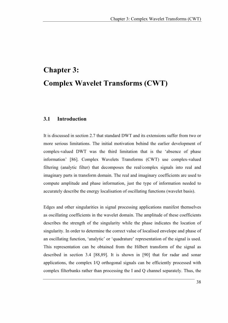
Recent developments in CWTs are classified into two important classes first
is, Redundant CWT (RCWT), and second is Non-Redundant CWT (NRCWT). The
important forms of RCWT include Kingsbury’s and Selesnick’s Dual-Tree DWT
(DT-DWT), whereas the important forms of NRCWT include Fernandes’s and
Spaendonck’s Projection based CWT (PCWT), and Orthogonal Hilbert transform
filterbank based CWT (OHCWT) respectively. All recent forms of CWTs try to
reduce two or more limitations of standard DWT with limited (or controllable)
redundancy, or without any redundancy. Potential applications such as Motion
estimation, Image fusion/registration, Denoising, Edge detection, and Texture
analysis are suggested for further investigation with RCWT. Directional and phase
based Compression is suggested for investigation with NRCWT.
Denoising and Edge detection applications are investigated with DT-DWTs.
Promising results are compared with other DWT extensions, and with the classical
approaches. After thorough investigations, it is proposed that by employing DT-
DWT for Motion estimation and NRCWT for Compression might significantly
improve the performance of the next generation video codecs.
vii

Acronyms 1-D One Dimensional
2-D Two Dimensional
FT Fourier Transform
DFT Discrete Fourier Transform
FFT Fast Fourier Transform
WT Wavelet Transform
DWT Discrete Wavelet Transform
MRA Multi-Resolution Analysis
PR Perfect Reconstruction
WP Wavelet Packet Transform
SWT Stationary Wavelet Transform
TFR Time Frequency Representation
STFT Short Time Fourier Transform
AWT Analog (Continuous) Wavelet Transform
CoWT Continuous (Analog) Wavelet Transform
CWT Complex Wavelet Transform
FIR Finite Impulse Response
GUI Graphical User Interface
SDW Symmetric Daubechies Wavelets
RCWT Redundant Complex Wavelet Transform
NRCWT Non Redundant Complex Wavelet Transform
DT-DWT Dual Tree Discrete Wavelet Transform
DT-DWT(K) Kingsbury’s Dual Tree Discrete Wavelet Transform
DT-DWT(S) Selesnick’s Dual Tree Discrete Wavelet Transform
DDWT Double Density Discrete Wavelet Transform
DDTWT Double Density Discrete Wavelet Transform
CDDWT Complex Double Density Wavelet Transform
PCWT Projection based Complex Wavelet Transform
viii

PCWT-CR Projection based Complex wavelet Transform with
Controllable Redundancy
PCWT-NR Projection based Complex wavelet Transform with No
Redundancy
OHCWT Orthogonal Hilbert Transform Filterbank based Complex
Wavelet Transform
MSE Mean Square Error
RMSE Root Mean Square Error
SNR Signal to Noise Ratio
PSNR Peak Signal to Noise Ratio
SURE Stein’s Unbiased Risk Estimator
MRI Magnetic Resonance Imaging
SAR Synthetic Aperture Radar
HMM Hidden Markov Model
STSA Short Time Spectrum Attenuation
STWA Short Time Wavelet Attenuation
MZ-MED Mallat and Zong’s Multiscale Edge Detection
ECG Electrocardiogram
FMED Fuzzy Multiscale Edge Detection
FWOMED Fuzzy Weighted Offset Multiscale Edge Detection
DBFMED Dual Basis Fuzzy Multiscale Edge Detection
CMED Complex Multiscale Edge Detection
IMED Imaginary Multiscale Edge Detection
FCMED Fuzzy Complex Multiscale Edge Detection
SFCMED Spatial Fuzzy Complex Multiscale Edge Detection
NFCMED Non-decimated Fuzzy Complex Multiscale Edge Detection
CBIR Content Based Image Retrieval
MSD Mean Square Distance
FOM Figure of Merit
ix

Table of Contents
Declaration v
Acknowledgement vi
Abstract vii
Acronyms viii
Table of Contents x
List of Figures xiv
List of Table xviii
1. Introduction 1 1.1 Introduction…………………………………………………………… 1
1.2 Motivation and Scope of Research……………………………………2
1.3 Organisation of Thesis……………………………………………….. 3
2. Wavelet Transforms (WT) 5 2.1 Introduction…………………………………………………………… 5
2.1.1 Wavelet Definition……………………………………………….. 5
2.1.2 Wavelet Characteristics………………………………………….. 6
2.1.3 Wavelet Analysis………………………………………………… 6
2.1.4 Wavelet History………………………………………………….. 6
2.1.5 Wavelet Terminology……………………………………………. 7
2.2 Evolution of Wavelet Transform…………………………………….. 8
2.2.1 Fourier Transform (FT)………………………………………….. 8
2.2.2 Short Time Fourier Transform (STFT)………………………….. 8
2.2.3 Wavelet Transform (WT)……………………………………….. 10
2.2.4 Comparative Visualisation………………………………………. 11
2.3 Theoretical Aspects of Wavelet Transform…………………………. 15
2.3.1 Continuous Wavelet Transform (CoWT)…………………………15
2.3.2 Discrete Wavelet Transform (DWT)…………………………….. 16
x

2.4 Implementation of DWT………………………………………………18
2.4.1 Multiresolution Analysis (MRA)………………………………… 18
2.4.2 Filterbank Implementation……………………………………….. 20
2.4.3 Perfect Reconstruction (PR)………………………………………22
2.5 Extensions of DWT…………………………………………………… 24
2.5.1 Two Dimensional DWT (2-D DWT)…………………………….. 25
2.5.2 Wavelet Packet Transform (WP)………………………………… 29
2.5.3 Stationary Wavelet Transform (SWT)…………………………… 32
2.6 Applications of Wavelet Transforms…………………………………33
2.7 Limitations of Wavelet Transforms…………………………………. 33
2.8 Summary………………………………………………………………. 36
3. Complex Wavelet Transforms (CWT) 38 3.1 Introduction…………………………………………………………… 38
3.2 Earlier Work………………………………………………………….. 39
3.3 Recent Developments…………………………………………………. 40
3.4 Analytic Filter…………………………………………………………. 43
3.5 Redundant Complex Wavelet Transforms (RCWT)……………….. 45
3.5.1 Introduction………………………………………………………. 45
3.5.2 Filterbank Structure of Dual-Tree DWT based CWT……….…… 46
3.5.3 Kingsbury’s Dual-Tree DWT (DT-DWT(K))…………………… 49
3.5.4 Selesnick’s Dual-Tree DWT (DT-DWT(S))…………………….. 56
3.5.5 Properties of DT-DWT……………………………………………58
3.6 Non-Redundant Complex wavelet Transforms (NRCWT)…………61
3.6.1 Introduction………………………………………………………. 61
3.6.2 Projection based CWT (PCWT)…………………………………. 62
3.6.2.1 Generic Structure……………………………………………62
3.6.2.2 Theory of Complex Projection ……………………………..63
3.6.2.3 Realisation of Complex Projection………………………… 64
3.6.2.4 Non-redundant Complex Projection……………………….. 67
3.6.3 PCWT with Controllable Redundancy (PCWT-CR)…………….. 69
3.6.4 PCWT with No-Redundancy (PCWT-NR)……………………… 70
xi
3.6.5 Orthogonal Hilbert Transform-
Filterbank based CWT (OHCWT) ………………………… 72
3.7 Advantages and Applications of CWT………………………………. 74
3.8 Summary………………………………………………………………. 76
4. Application I – Denoising 80 4.1 Introduction…………………………………………………………… 80
4.2 Wavelet Shrinkage Denoising…………………………………………81
4.2.1 Basic Concept……………………………………………………. 81
4.2.2 Shrinkage Strategies……………………………………………… 82
4.3 1-D Denoising…………………………………………………………. 83
4.3.1 Signal and Noise Model………………………………………….. 83
4.3.2 Shrinkage Strategy……………………………………………….. 84
4.3.3 Algorithm………………………………………………………… 84
4.3.4 Performance Measure……………………………………………. 85
4.3.5 Results and Discussion……………………………………………85
4.4 Audio Signal Denoising………………………………………………..92
4.4.1 WT for Audio Signals……………………………………………. 92
4.4.2 Denoising Model…………………………………………………. 92
4.4.3 Shrinkage Strategies……………………………………………… 93
4.4.4 Performance Measure……………………………………………..94
4.4.5 Results and Discussion……………………………………………94
4.5 2-D Denoising…………………………………………………………. 98
4.5.1 Image and Noise Model………………………………………….. 98
4.5.2 Shrinkage Strategy……………………………………………….. 98
4.5.3 Algorithm………………………………………………………… 98
4.5.4 Performance Measure……………………………………………. 99
4.5.5 Results and Discussion……………………………………………99
4.6 Conclusion…………………………………………………………….. 117
5. Application II - Edge Detection 118 5.1 Introduction…………………………………………………………… 118
xii

5.2 Edge Detection Approaches………………………………………….. 119
5.2.1 Classical Approaches…………………………………………….. 119
5.2.2 Multiscale Approaches…………………………………………… 120
5.3 1-D Edge Detection…………………………………………………… 121
5.3.1 Review of Existing Approaches…………………………………..121
5.3.2 Edge Model………………………………………………………. 122
5.3.3 Multiscale Decomposition……………………………………….. 122
5.3.4 FMED (Fuzzy Multiscale Edge Detection) Algorithms…………. 123
5.3.5 CMED (Complex Multiscale Edge Detection) Algorithms……… 126
5.3.6 Performance Measure……………………………………………. 127
5.3.7 Results and Discussion…………………………………………... 128
5.4 2-D Edge Detection…………………………………………………… 137
5.4.1 Basic Approach………………………………………………….. 137
5.4.2 Algorithms……………………………………………………….. 138
5.4.2.1 WT based Algorithm………………………………………..138
5.4.2.2 CWT based Algorithm……………………………………... 138
5.4.3 Performance Measure……………………………………………. 139
5.4.4 Results and Discussion…………………………………………... 140
5.5 Conclusion…………………………………………………………….. 142
6. Conclusions and Future Scope 143 6.1 Conclusions……………………………………………………………. 143
6.2 Future Scope…………………………………………………………... 146
Appendix A 148
Appendix B 150
Appendix C 152
References 153
xiii

List of Figures
Figure 2.1 Representation of a wave (a), and a wavelet (b)………………….. 5
Figure 2.2 (a) Uniform division of frequency with constant bandwidth in
STFT, (b) logarithmic division of frequency with constant-Q in
WT…………………………………………………………………
10
Figure 2.3 Comparative visualisation of time-frequency representation of an
arbitrary non-stationary signal in various transform domains…….
12
Figure 2.4 Two signals x1(t) and x2(t) and their FFTs………………………... 13
Figure 2.5 Spectrograms and scalograms of signals x1(t) and x2(t)…………... 14
Figure 2.6 Standard DWT on dyadic time-scale grid………………………… 17
Figure 2.7 Nested vector spaces spanned by scaling and wavelet basis……… 18
Figure 2.8 Two-channel, three-level analysis filterbank with 1-D DWT…….. 21
Figure 2.9 Two-channel, three-level synthesis filterbank with 1-D DWT…… 21
Figure 2.10 A simple 2-channel filterbank model……………………………... 22
Figure 2.11 Single level analysis filterbank for 2-D DWT……………………. 25
Figure 2.12 Multilevel decomposition hierarchy of an image with 2-D DWT... 26
Figure 2.13 Frequency plane partitioning with 2-D DWT…………………….. 27
Figure 2.14 (a) Test image ‘Pattern’, (b) single level 2-D DWT decomposition
of the same………………………………………………………...
28
Figure 2.15 Wavelet packet transform:(a) binary-tree decomposition, (b) time-
frequency tiling of basis…………………………………………...
30
Figure 2.16 Vector subspaces for WP…………………………………………. 31
Figure 2.17 Uniform frequency division for WP………………………………. 31
Figure 2.18 Flexible representation with WP: either with boxes or with circles 31
Figure 2.19 Three level decomposition with SWT…………………………….. 32
Figure 2.20 Shift-sensitivity of standard 1-D DWT…………………………… 34
Figure 2.21 Directionality of standard 2D DWT………………………………. 35
Figure 2.22 Presentation of (a) real, and (b) analytic wavelets……………….. 36
Figure 3.1 Hilbert Transform in (a) polar form, (b) frequency domain……… 43
Figure 3.2 Spectral representation of (a) original signal f(t), (b) analytic signal
xiv

x(t)………………………………………………………….. 44
Figure 3.3 Interpretation of an analytic filter by 2-real filters………………... 45
Figure 3.4 (a) Analysis filterbank for 1-D DT-DWT, (b) synthesis filterbank
for 1-D DT-DWT…………………………………………………
47
Figure 3.5 Filterbank structure for 2-D DT-DWT……………………………. 48
Figure 3.6 Filterbank structure of tree-a of figure 3.5………………………... 49
Figure 3.7 Analysis tree using odd-even filters………………………………. 50
Figure 3.8 Analysis tree using Q-shift filters…………………………………. 50
Figure 3.9 Modelling of DT-DWT(K) filter structure for deriving the shift-
invariance constraints……………………………………………...
51
Figure 3.10 Shift-invariance property of 1-D DT-DWT………………………. 59
Figure 3.11 Directionality of 2-D DT-DWT…………………………………... 59
Figure 3.12 3-D representation of 12 wavelets of DT-DWT…………………... 60
Figure 3.13 A complex wavelet as a quadrature combination of real and
imaginary wavelets for 1-D DT-DWT…………………………….
61
Figure 3.14 Generic implementation of PCWT………………………………... 63
Figure 3.15 Realisable complex projection in softy-space…………………….. 65
Figure 3.16 |H+(ω)|, the magnitude response of complex projection filter h+…. 66
Figure 3.17 Relation between function spaces………………………………… 66
Figure 3.18 Non-redundant complex projection……………………………….. 67
Figure 3.19 The relationship between non-redundant mapping +H~ and Softy-
space mapping h+…………………………………………………..
68
Figure 3.20 Implementation of realisable PCWT: PCWT-CR………………… 69
Figure 3.21 Realisation of non-redundant mapping…………………………… 70
Figure 3.22 3-band filterbank structure for 1-D OHCWT……………………... 72
Figure 3.23 Single level analysis filterbank equivalence of 1-D OHCWT for
real signal as shown in figure (3.22)………………………………
73
Figure 3.24 Three possible ways of implementing CWT for natural signals….. 79
Figure 4.1 Thresholding functions; (a) linear, (b) hard, (c) soft……………… 82
Figure 4.2 (a) Denoising of signal ‘blocks’ with standard DWT, WP and
SWT, (b) Denoising of signal ‘blocks’ with redundant CWT, DT-
DWT(S) and DT-DWT(K)………………………………………...
90
91
xv

Figure 4.3 Block diagram of STWA (short time wavelet attenuation) method.. 92
Figure 4.4 Spectrograms of audio signals with standard DWT based
denoising……………………………………………………………
96
Figure 4.5 Spectrograms of audio signals with DT-DWT(K) based denoising.. 97
Figure 4.6 Conventional filtering methods for denoising of ‘Lenna’ image
with reference to tables (4.7) and (4.8)……………………………..
107
Figure 4.7 Wavelet Transform based methods for denoising of ‘Lenna’ image
with reference to tables (4.7) to (4.9)………………………………
108
Figure 4.8 Threshold vs MSE for determination of optimum threshold value
for all wavelet based methods. Image for denoising is ‘Lenna’ with
reference to table (4.9)……………………………………………...
109
Figure 4.9 Conventional filtering methods for denoising of ‘Lenna’ image
with reference to tables (4.10) and (4.11)…………………………..
110
Figure 4.10 Wavelet Transform based methods for denoising of ‘Lenna’ image
with reference to tables (4.10) to (4.12)……………………………
111
Figure 4.11 Threshold Vs MSE for determination of optimum threshold value
for all wavelet based methods. Image for denoising is ‘Lenna’ with
reference to table (4.12)…………………………………………….
112
Figure 4.12 DWT based denoising of ‘Lenna’ image using hard and soft
thresholding with reference to tables (4.10) to (4.12)……………...
113
Figure 4.13 SWT based denoising of ‘Lenna’ image using hard and soft
thresholding with reference to tables (4.10) to (4.12)……………...
114
Figure 4.14 DT-DWT(K) based denoising of ‘Lenna’ image using hard and
soft thresholding with reference to tables (4.10) to (4.12)…………
115
Figure 4.15 DT-DWT(S) based denoising of ‘Lenna’ image using hard and
soft thresholding with reference to tables (4.10) to (4.12)…………
116
Figure 5.1 Generalised step edge model………………………………………. 122
Figure 5.2 Cubic spline smoothing function φ(t) and its derivative ψ(t) =
d/dt(φ(t))……………………………………………………………
123
Figure 5.3 1-D edge detection with FMED (‘cubic’) with σ =0.6 and ∆=5…... 133
Figure 5.4 J level wavelet coefficients (left) and their only positive parts
(right) with FMED(‘cubic’) under the noise of σ =0.6 and slope of
xvi

∆=5………………………………………………………………… 133
Figure 5.5 J level fuzzy subsets (left) and their corresponding 2 to J level
fuzzy intersection (right) for the computation of minimum fuzzy
set (right top) employing FMED (‘cubic’) under the noise of σ
=0.6 and slope of ∆=5………………………………………………
134
Figure 5.6 1-D edge detection with CMED: σ =0.6 and ∆=5…………………. 134
Figure 5.7 J level of decimated real and imaginary coefficients with CMED:
σ =0.6 and ∆=5……………………………………………………..
135
Figure 5.8 J level of decimated original and modified (inverted and left cyclic
shift of 1 sample for levels 2 to J ) real coefficients with CMED:
σ =0.6 and ∆=5……………………………………………………..
135
Figure 5.9 J level of interpolated modified real and original imaginary
coefficients with CMED: σ =0.6 and ∆=5…………………………
136
Figure 5.10 J level of complex magnitude coefficients (left) and fuzzy subsets
of complex magnitudes (right). Top left shows detected edge with
complex magnitude (at level 5) and top right shows detected edge
with fuzzy subset (at level 5) employing CMED: σ =0.6 and ∆=5...
136
Figure 5.11 2-D edge detection with conventional edge operators…………….. 140
Figure 5.12 2-D edge detection with wavelet based methods………………….. 141
xvii
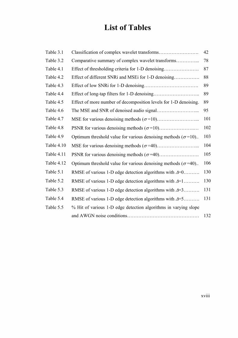
List of Tables
Table 3.1 Classification of complex wavelet transforms……………………. 42
Table 3.2 Comparative summary of complex wavelet transforms…………... 78
Table 4.1 Effect of thresholding criteria for 1-D denoising…………………. 87
Table 4.2 Effect of different SNRi and MSEi for 1-D denoising……………. 88
Table 4.3 Effect of low SNRi for 1-D denoising……………………………. 89
Table 4.4 Effect of long-tap filters for 1-D denoising……………………….. 89
Table 4.5 Effect of more number of decomposition levels for 1-D denoising. 89
Table 4.6 The MSE and SNR of denoised audio signal……………………... 95
Table 4.7 MSE for various denoising methods (σ =10)……………………... 101
Table 4.8 PSNR for various denoising methods (σ =10)………………….… 102
Table 4.9 Optimum threshold value for various denoising methods (σ =10).. 103
Table 4.10 MSE for various denoising methods (σ =40)……………………... 104
Table 4.11 PSNR for various denoising methods (σ =40)……………………. 105
Table 4.12 Optimum threshold value for various denoising methods (σ =40).. 106
Table 5.1 RMSE of various 1-D edge detection algorithms with ∆=0………. 130
Table 5.2 RMSE of various 1-D edge detection algorithms with ∆=1………. 130
Table 5.3 RMSE of various 1-D edge detection algorithms with ∆=3………. 131
Table 5.4 RMSE of various 1-D edge detection algorithms with ∆=5………. 131
Table 5.5 % Hit of various 1-D edge detection algorithms in varying slope
and AWGN noise conditions………………………………………
132
xviii

Chapter 1: Introduction
Chapter 1:
Introduction
1.1 Introduction
Fourier Transform (FT) with its fast algorithms (FFT) is an important tool for
analysis and processing of many natural signals. FT has certain limitations to
characterise many natural signals, which are non-stationary (e.g. speech). Though a
time varying, overlapping window based FT namely STFT (Short Time FT) is well
known for speech processing applications, a new time-scale based Wavelet
Transform (WT) is a powerful mathematical tool for non-stationary signals.
WT uses a set of damped oscillating functions known as wavelet basis. WT in
its continuous (analog) form is represented as CoWT. CoWT with various
deterministic or non-deterministic basis is a more effective representation of signals
for analysis as well as characterisation. Continuous wavelet transform (CoWT) is
powerful in singularity detection. A discrete and fast implementation of CoWT
(generally with real valued basis) is known as the standard DWT (Discrete Wavelet
Transform).
With standard DWT, signal has a same data size in transform domain and
therefore it is a non-redundant transform. Standard DWT can be implemented
through a simple filterbank structure of recursive FIR filters. A very important
property; Multiresolution Analysis (MRA) allows DWT to view and process 1

Chapter 1: Introduction different signals at various resolution levels. The advantages such as non-
redundancy, fast and simple implementation with digital filters using micro-
computers, and MRA capability popularised the DWT in many signal processing
applications since last decade. Many researches have successfully applied and proved
the advantages of DWT for signal denoising and compression in a number of diverse
fields.
1.2 Motivation and Scope of Research
Though standard DWT is a powerful tool for analysis and processing of many real-
world signals and images, it suffers from three major disadvantages, (1) Shift-
sensitivity, (2) Poor directionality, and (3) Lack of phase information. These
disadvantages severely restrict its scope for certain signal and image processing
applications (e.g. edge detection, image registration/segmentation, motion
estimation).
Other extensions of standard DWT such as Wavelet Packet Transform (WP)
and Stationary Wavelet Transform (SWT) reduce only the first disadvantage of shift-
sensitivity but with the cost of very high redundancy and involved computation.
Recent research suggests the possibility of reducing two or more above-mentioned
disadvantages using different forms of Complex Wavelet Transforms (CWT)
[93,98,101,103] with only limited (and controllable) redundancy and moderate
computational complexity.
The objectives of research in this thesis include:
1. Review of Wavelet Transforms: History, Theory, Various forms of WTs and
their properties, and Applications.
2. Thorough study of Complex Wavelet Transforms (CWT): History, Theory,
Various forms, Properties, and Investigations for potential applications.
2
Chapter 1: Introduction 3. Comprehensive and collective analysis of recently proposed CWTs, and a
comparison with existing forms of WTs.
4. Implementation: Practical realisation of various CWTs and WTs through
individual Matlab simulations. Review of selected applications like denoising
and edge detection. Individual implementation of selected application with
suitable WTs and CWTs. Incorporating novel ideas culminating in the
original and novel outcomes. Statistical validation of original results.
5. Comparative study: Critical evaluation of the original results obtained from
individual implementations of existing and novel algorithms for selected
applications using various forms of WTs and CWTs.
1.3 Organisation of Thesis
The thesis is organised in to six chapters as follows:
Chapter 1 is an introduction with the comprehensive description of the central
theme of this research. A systematic organisation of thesis is also presented.
Chapter 2 is a detailed review of Wavelet Transforms (WT). A brief history,
evolution and fundaments of wavelet transforms are presented. The structure of fast
and reversible implementation of standard DWT (Discrete wavelet Transform)
through filterbank is explained. Concept of separable and multidimensional DWT as
an extension of 1-D DWT is described. Other important variants of WTs like SWT
(Stationary wavelet Transforms) and WP (Wavelet Packet Transforms) with their
properties are reviewed. Finally, the applications and limitations of the popular
standard DWT are enlisted.
Chapter 3 is the heart of this thesis. It presents a thorough study of CWT
(Complex wavelet Transforms). The history, evolution and recent advances in the
field of CWTs are comprehensively analysed. Recent developments and newer
3

Chapter 1: Introduction extensions of CWTs with their theories, structures and properties are critically
explored. Advantages and limitations of various CWTs are analysed through
individual implementations and simulations. Potential applications of various forms
of CWTs are suggested after thorough investigations.
Chapter 4 and chapter 5 are about practical implementations and simulations
carried out with various WTs (reviewed in chapter 2) and CWTs (investigated in
chapter 3). Key signal and image processing applications such as Denoising and
Edge-detection are thoroughly reviewed. In chapter 4, Denoising application is
explored in both 1-D and 2-D cases with WTs, and redundant CWTs (i.e. DT-DWT).
In chapter 5, Edge-detection application is explored in similar manner.
Individual simulations with WTs and CWTs algorithms are carried out for the
mentioned applications and performances are compared with other conventional
algorithms. Some novel ideas are incorporated in existing algorithms and available
results are presented after statistical validation.
Chapter 6 is the summary of investigation on ‘complex wavelet transforms
and their applications’. The advantages and limitations of CWTs over other WTs for
the selected applications (namely denoising and edge-detection) are concluded.
Future directions are given for further investigations using CWTs in other relevant
applications (such as Motion estimation and Compression for video coding).
4

Chapter2: Wavelet Transforms (WT)
Chapter 2:
Wavelet Transforms (WT)
2.1 Introduction
2.1.1 Wavelet Definition
A ‘wavelet’ is a small wave which has its energy concentrated in time. It has an
oscillating wavelike characteristic but also has the ability to allow simultaneous time
and frequency analysis and it is a suitable tool for transient, non-stationary or time-
varying phenomena [1,2].
Figure 2.1: Representation of a wave (a), and a wavelet (b)
5

Chapter2: Wavelet Transforms (WT) 2.1.2 Wavelet Characteristics
The difference between wave (sinusoids) and wavelet is shown in figure (2.1).
Waves are smooth, predictable and everlasting, whereas wavelets are of limited
duration, irregular and may be asymmetric. Waves are used as deterministic basis
functions in Fourier analysis for the expansion of functions (signals), which are time-
invariant, or stationary. The important characteristic of wavelets is that they can
serve as deterministic or non-deterministic basis for generation and analysis of the
most natural signals to provide better time-frequency representation, which is not
possible with waves using conventional Fourier analysis.
2.1.3 Wavelet Analysis
The wavelet analysis procedure is to adopt a wavelet prototype function, called an
‘analysing wavelet’ or ‘mother wavelet’. Temporal analysis is performed with a
contracted, high frequency version of the prototype wavelet, while frequency
analysis is performed with a dilated, low frequency version of the same wavelet [12].
Mathematical formulation of signal expansion using wavelets gives Wavelet
Transform (WT) pair, which is analogous to the Fourier Transform (FT) pair.
Discrete-time and discrete-parameter version of WT is termed as Discrete Wavelet
Transform (DWT). DWT can be viewed in a similar framework of Discrete Fourier
Transform (DFT) with its efficient implementation through fast filterbank algorithms
similar to Fast Fourier Transform (FFT) algorithms [1].
2.1.4 Wavelet History
Wavelet theory has been developed as a unifying framework only recently, although
similar ideas and constructions took place as early as the beginning of the century
[3,4]. The idea of looking at a signal at various scales and analyzing it with various
resolutions has in fact emerged independently in many different fields of
mathematics, physics and engineering. In mid-eighties, researchers of the ‘French
school’ [5-7] built strong mathematical foundation around the subject and named
6

Chapter2: Wavelet Transforms (WT) their work ‘ondeletts’ (wavelets). Brief history of early research on wavelets can be
found in [8]. A very good overview of the philosophy of wavelet analysis and history
of its development is given in [9]. Introductory tutorial articles on wavelets are [10-
13]. Readable books on wavelet theory and applications are [1,2,14-25].
2.1.5 Wavelet Terminology
The applications of wavelets to signal processing can be attributed to [26-27].
Wavelet theory is closely related to filter bank theory [15,28]. In [28] the concept of
Multiresolution Analysis (MRA) was introduced leading to an implementation of
DWT with octave-band filterbank, while [26] showed that under certain condition
filter bank converges to orthonormal wavelet bases. Generation of various wavelet
families (Daubecheis, Coiflets, Symlets etc.) through modifications in
parameterization of wavelets availed some useful properties such as compact-
support, symmetry, regularity, and smoothness [24].
The wavelet systems with biorthogonalily gives flexibility [29,30],
overcompleteness removes certain disadvantages of DWT [24,31], and Perfect
Reconstruction (PR) filterbank implementation is utmost essential for retrieval of
original signal [15,32-33]. Wavelet Packet Transform (WP) is an efficient
decomposition of filterbank [65-68]. All these newer techniques have broaden the
scope of wavelets in various signal and image processing applications [11,20,34-36].
Section 2.2 leads towards the evolution of wavelet transform through various
time-frequency representations. Section 2.3 describes the theoretical aspects of the
WT in continuous and discrete domains, whereas section 2.4 deals with the
implementation aspects of the WT. Section 2.5 introduces the useful extensions of
generic WT in discrete domain. Sections 2.6 and 2.7 are about the applications and
limitations of various WTs. Section 2.8 is a summary highlighting the need for an
alternate form of WT namely Complex Wavelet Transform (CWT).
7
Chapter2: Wavelet Transforms (WT) 2.2 Evolution of Wavelet Transform
The need of simultaneous representation and localisation of both time and frequency
for non-stationary signals (e.g. music, speech, images) led toward the evolution of
wavelet transform from the popular Fourier transform. Different ‘time-frequency
representations’ (TFR) are very informative in understanding and modelling of WT
[37-39].
2.2.1 Fourier Transform (FT)
Fourier transform is a well-known mathematical tool to transform time-domain
signal to frequency-domain for efficient extraction of information and it is reversible
also. For a signal x(t), the FT is given by:
dtetxfX tfj π2)()( −∞
∞−∫= (2.1)
Though FT has a great ability to capture signal’s frequency content as long as x(t) is
composed of few stationary components (e.g. sine waves). However, any abrupt
change in time for non-stationary signal x(t) is spread out over the whole frequency
axis in X(f). Hence the time-domain signal sampled with Dirac-delta function is
highly localised in time but spills over entire frequency band and vice versa. The
limitation of FT is that it cannot offer both time and frequency localisation of a signal
at the same time.
2.2.2 Short Time Fourier Transform (STFT)
To overcome the limitations of the standard FT, Gabor [39] introduced the initial
concept of Short Time Fourier Transform (STFT). The advantage of STFT is that it
uses an arbitrary but fixed-length window g(t) for analysis, over which the actual
nonstationary signal is assumed to be approximately stationary. The STFT
decomposes such a pseudo-stationary signal x(t) into a two dimensional time-
8

Chapter2: Wavelet Transforms (WT) frequency representation S(τ , f) using that sliding window g(t) at different times τ .
Thus the FT of windowed signal x(t) g*(t-τ) yields STFT as:
STFTx (τ , f ) = x(t) g∫∞
∞−
*(t-τ) e-j2π f t dt (2.2)
Filterbank interpretation is an alternative way of seeing ‘windowing of the
signal’ viewpoint of STFT [41,42]. With the modulated filterbank, a signal can be
seen as passing through a bandpass filter centred at frequency f with an impulse
response of the window function modulated to that frequency. The division of
frequency is uniform as shown in figure (2.2 a).
From this dual interpretation, a possible drawback related to time-frequency
resolution of STFT can be shown through ‘Heisenberg’s uncertainty principle’
[2,43,44]. For a window g(t) and its Fourier transform G(f), both centred around the
origin in time as well as in frequency, that is satisfying ∫ t g(t)2dt =0 and ∫ f
G(f)2df =0. Then the spreads in time and frequency are defined as:
∆t2 =
∫
∫∞
∞−
∞
∞−
dttg
dttgt
2
22
)(
)(
∆f2 =
∫
∫∞
∞−
∞
∞−
dffG
dffGf
2
22
)(
)( (2.3)
Thus, the time-frequency resolution for STFT is lower bounded by their product as:
Time-Bandwidth product = ∆t ∆f ≥ π41 (2.4)
9
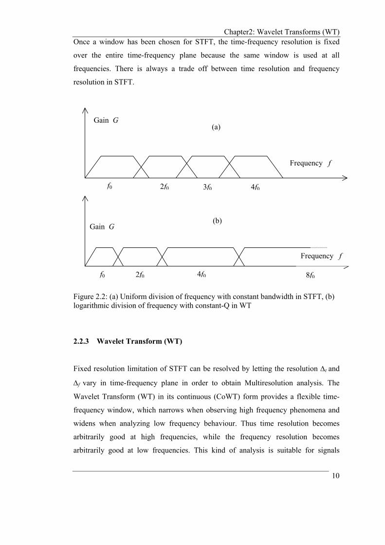
Chapter2: Wavelet Transforms (WT) Once a window has been chosen for STFT, the time-frequency resolution is fixed
over the entire time-frequency plane because the same window is used at all
frequencies. There is always a trade off between time resolution and frequency
resolution in STFT.
Gain G
Gain G
Frequency f
f0 2f0 3f0 4f0
f0 2f0 4f0 8f0
Frequency f
(a)
(b)
Figure 2.2: (a) Uniform division of frequency with constant bandwidth in STFT, (b) logarithmic division of frequency with constant-Q in WT
2.2.3 Wavelet Transform (WT)
Fixed resolution limitation of STFT can be resolved by letting the resolution ∆t and
∆f vary in time-frequency plane in order to obtain Multiresolution analysis. The
Wavelet Transform (WT) in its continuous (CoWT) form provides a flexible time-
frequency window, which narrows when observing high frequency phenomena and
widens when analyzing low frequency behaviour. Thus time resolution becomes
arbitrarily good at high frequencies, while the frequency resolution becomes
arbitrarily good at low frequencies. This kind of analysis is suitable for signals
10

Chapter2: Wavelet Transforms (WT) composed of high frequency components with short duration and low frequency
components with long duration, which is often the case in practical situations [11].
When analysis is viewed as a filterbank, the WT, generally termed as
standard Discrete Wavelet Transform (DWT), is seen as a composition of bandpass
filters with constant relative bandwidth (constant–Q) such that ∆f /f is always
constant. As ∆f changes with frequencies, corresponding time resolution ∆t also
changes so as to satisfy the uncertainty condition. The frequency responses of
bandpass filters are logarithmically spread over frequency as shown in figure (2.2 b).
A generalisation of the concept of changing resolution at different frequencies is
obtained with so-called Wavelet Packet Transform (WP) [67], where arbitrary time-
frequency resolutions are chosen depending on the signal. More detailed description
about the WT is given in subsequent sections of this chapter.
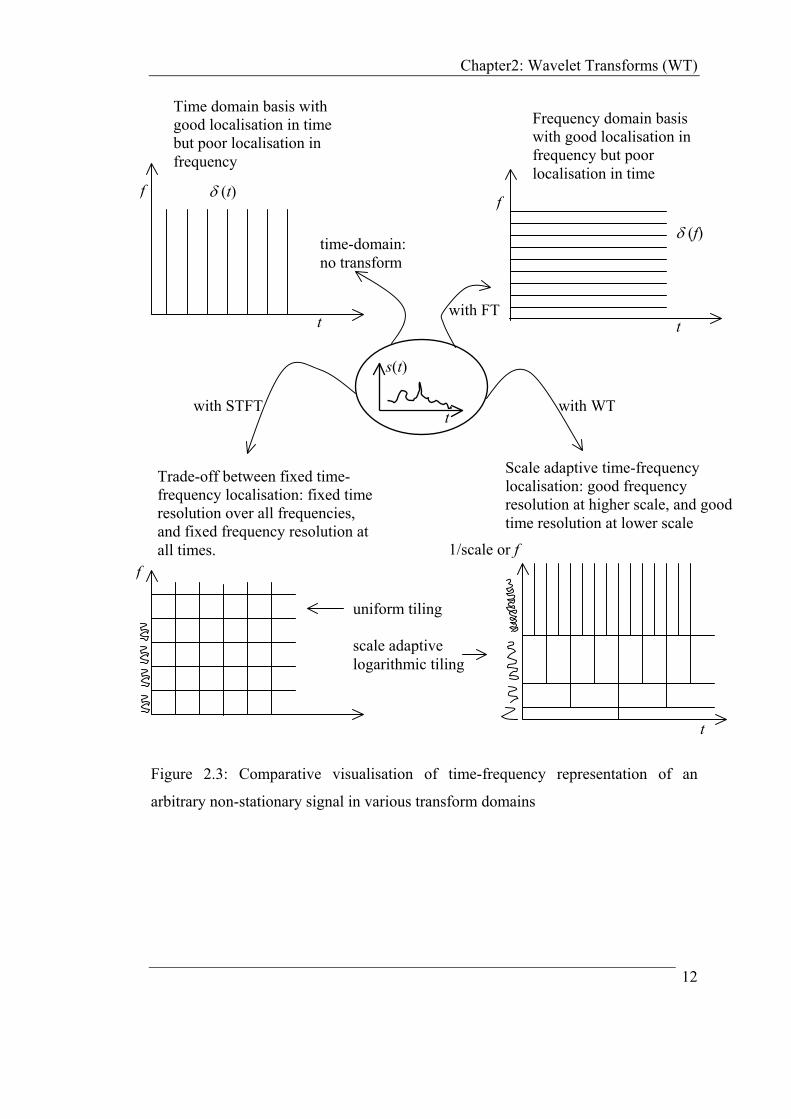
2.2.4 Comparative Visualisation
A comprehensive visualization of various time-frequency representations, shown in
figure (2.3), demonstrates the time-frequency resolution for a given signal in various
transform domains with their corresponding basis functions [1].
The time-frequency representation problem is illustrated with Matlab
simulations in figure (2.4) and figure (2.5) using two signals x1(t) and x2(t). The
signals are analysed through their corresponding FTs with FFTs, through STFTs with
spectrograms, and through their CoWTs with scalograms [25]. Signal x1(t) =
sin(2π10t)+ sin(2π35t)+ sin(2π50t) is a stationary signal composed of three
sinusoids of 10Hz, 35Hz, and 50Hz. Signal x2(t) is non-stationary, which contains the
same three distinct frequency components but over three adjoining time slots such
that only one frequency component is present in a particular time interval. In both
cases, the FFT picks up frequency contents very well but it fails to demonstrate the
time varying nature of signal x2(t).
11
Chapter2: Wavelet Transforms (WT)
s(t)
t
δ (t)
t
δ (f)
f
t
t
1/scale or f
Time domain basis with good localisation in time but poor localisation in frequency
Frequency domain basis with good localisation in frequency but poor localisation in time
Trade-off between fixed time- frequency localisation: fixed time resolution over all frequencies, and fixed frequency resolution at all times.
uniform tiling scale adaptive logarithmic tiling
with FT
time-domain: no transform
with WT with STFT
f
f
Scale adaptive time-frequency localisation: good frequency resolution at higher scale, and good time resolution at lower scale
Figure 2.3: Comparative visualisation of time-frequency representation of an
arbitrary non-stationary signal in various transform domains
12

Chapter2: Wavelet Transforms (WT)
Figure 2.4: Two signals x1(t) and x2(t) and their FFTs
13

Chapter2: Wavelet Transforms (WT)
Figure 2.5: Spectrograms and scalograms of signals x1(t) and x2(t) 14

Chapter2: Wavelet Transforms (WT) Spectrograms (modulus of STFT) and scalograms (modulus of CoWT) for both
signals x1(t) and x2(t) are shown in figure (2.5), which show the stationarity of x1(t)
and the time-varying nature of signal x2(t). Spectrogram has fixed resolution for x2(t),
where as scalogram gives good frequency- resolution at lower frequency (high scale)
and limited frequency-resolution at high frequency (low scale) for the same signal
x2(t). But the time localization is good at higher frequency (low scale) compared to
low frequency (high scale).
2.3 Theoretical Aspects of Wavelet Transform Wavelet transform can represented in continuous as well as in discrete domain as
follows.
2.3.1 Continuous Wavelet Transform (CoWT)
For a prototype function ψ (t) ∈ L2(ℜ) called the mother wavelet, the family of
functions can be obtained by shifting and scaling this ψ (t) as:
ψ a,b(t) = a
1 ψ (a
bt − ) , where a , b ∈ ℜ ( a > 0) (2.5)
Parameter a is a scaling factor and b is shifting factor. Normalization ensures that ||ψ
a,b(t)|| = ||ψ (t)||. The mother wavelet has to satisfy the following admissibility
condition
Cψ = ∫∞
∞−
Ψωω 2|)(| dω < ∞ , where )(ωΨ is the Fourier transform of ψ (t).
In practice )(ωΨ will have sufficient decay, so that the admissibility condition
reduces to
∫∞
∞−
)(tψ dt = (0) = 0. (2.6) Ψ
Thus, the wavelet will have bandpass behaviour.
15

Chapter2: Wavelet Transforms (WT) The ‘continuous wavelet transform’ (CoWT) of a function f (t) ∈ ℜ is then
defined as:
CoWTf (a,b) = ψ*∫∞
∞−
a,b(t) f (t) dt = ⟨ψ a,b(t), f (t) ⟩ (2.7)
A basis function ψa,b(t), can also be seen as filterbank impulse response. With the
increase in scale (a >1), the function ψ a,b(t) is dilated in time to focus on long-time
behaviour of associated signal f (t) with it. In general, very large scale means global
view of the signal while very small-scale means a detailed view of the signal. A
related notion with scale is resolution. The resolution of a signal is limited to its
frequency content. The scale change of continuous time signals in CoWT does not
alter their resolution, since the scale change can be reversed [11].
Through continuous wavelet transform analysis, a set of wavelet coefficients
{CoWTf (a,b)} are obtained. These coefficients indicate how close the signal is to a
particular basis function. Since, the CoWT behaves like orthonormal basis
decomposition, it can be shown that it is isometric [6], i.e. it preserves energy. Hence
the function f(t) can be recovered from its transform by the following reconstruction
formula:
f (t) = ψC1
2, )(),(a
dbdatbaCWT baf∫ ∫∞
∞−
∞
∞−
ψ (2.8)
2.3.2 Discrete Wavelet Transform (DWT)
The CoWT has the drawbacks of redundancy and impracticability with digital
computers. As parameters (a, b) take continuous values, the resulting CoWT is a
very redundant representation, and impracticability is the result of redundancy.
Therefore, the scale and shift parameters are evaluated on a discrete grid of time-
scale plane leading to a discrete set of continuous basis functions [38]. The
discretization is performed by setting 16
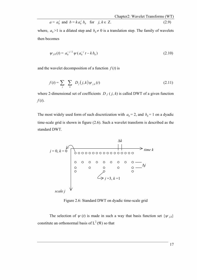
Chapter2: Wavelet Transforms (WT) a = a and b = k for j, k ∈ Ζ. (2.9) j
0ja0 0b
where, >1 is a dilated step and b ≠ 0 is a translation step. The family of wavelets
then becomes
0a 0
ψ j,k (t) = ψ ( ) (2.10) 2/0
ja −00 bkta j −−
and the wavelet decomposition of a function f (t) is
f (t) = ( ) )(, , tkjD kjj k
f ψ∑ ∑ (2.11)
where 2-dimensional set of coefficients D f ( j, k) is called DWT of a given function
f (t).
The most widely used form of such discretization with a = 2, and = 1 on a dyadic
time-scale grid is shown in figure (2.6). Such a wavelet transform is described as the
standard DWT.
0 0b
scale j
time k
j =3, k =1
j = 0, k = 0
∆j
∆k
Figure 2.6: Standard DWT on dyadic time-scale grid
The selection of ψ (t) is made in such a way that basis function set {ψ j,k}
constitute an orthonormal basis of L2 (ℜ) so that
17
Chapter2: Wavelet Transforms (WT)
D f (j, k) = = ⟨∫∞
∞−
dttftkj )()(*,ψ )()(, tftkjψ ⟩ (2.12)
Several such wavelet bases have been reported in literature [45-48] to evaluate f (t)
using the summation of finite basis over index j and k with finite DWT coefficients
with almost no error. All these wavelets can be derived with an arbitrary resolution
and with finite DWT coefficients.
2.4 Implementation of DWT The practical usefulness of DWT comes from its Multi-Resolution Analysis (MRA)
ability [48-50], and efficient Perfect Reconstruction (PR) filterbank structures.
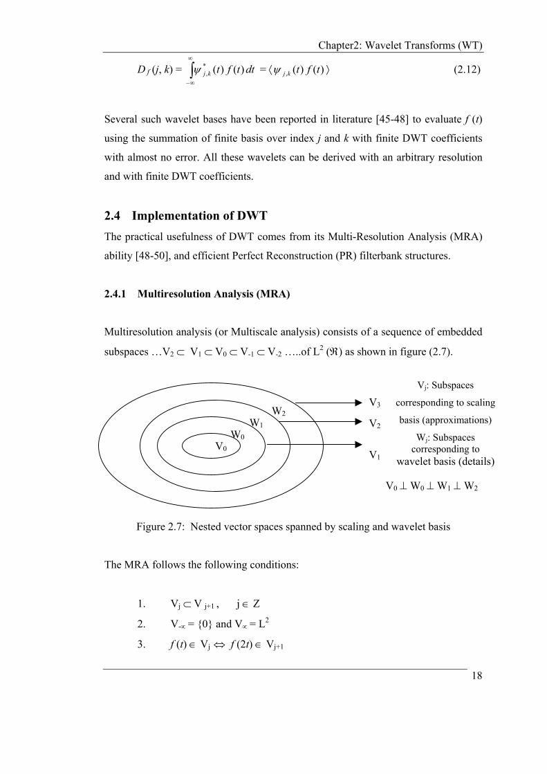
2.4.1 Multiresolution Analysis (MRA)
Multiresolution analysis (or Multiscale analysis) consists of a sequence of embedded
subspaces …V2 ⊂ V1 ⊂ V0 ⊂ V-1 ⊂ V-2 …..of L2 (ℜ) as shown in figure (2.7).
W2 W1
W0V0 V1
V2
V3 Vj: Subspaces
corresponding to scaling
basis (approximations)
Wj: Subspaces corresponding to
wavelet basis (details)
V0 ⊥ W0 ⊥ W1 ⊥ W2
Figure 2.7: Nested vector spaces spanned by scaling and wavelet basis
The MRA follows the following conditions:
1. Vj ⊂ V j+1 , j ∈ Ζ
2. V-∝ = {0} and V∝ = L2
3. f (t) ∈ Vj ⇔ f (2t) ∈ Vj+1
18
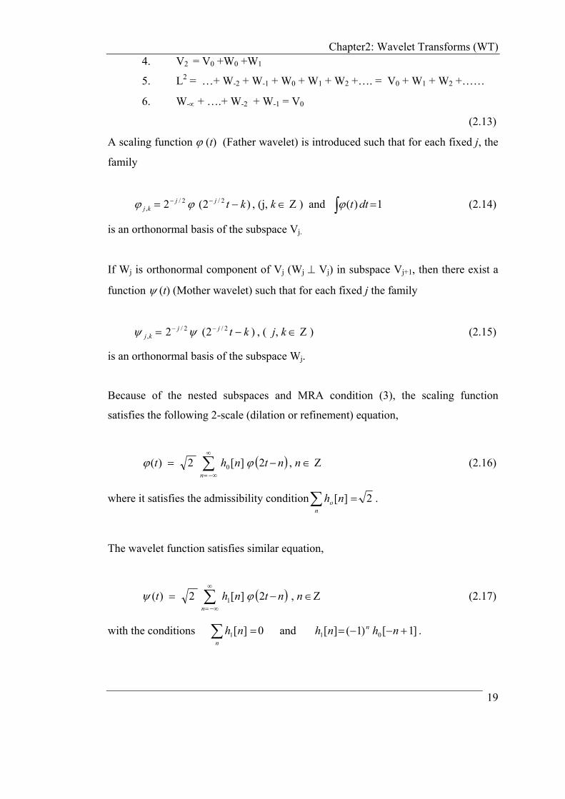
Chapter2: Wavelet Transforms (WT) 4. V2 = V0 +W0 +W1
5. L2 = …+ W-2 + W-1 + W0 + W1 + W2 +…. = V0 + W1 + W2 +……
6. W-∝ + ….+ W-2 + W-1 = V0
(2.13)
A scaling function ϕ (t) (Father wavelet) is introduced such that for each fixed j, the
family
, (j, k ∈ Ζ ) and )2(2 2/2/, ktjjkj −= −− ϕϕ ∫ =1)( dttϕ (2.14)
is an orthonormal basis of the subspace Vj.
If Wj is orthonormal component of Vj (Wj ⊥ Vj) in subspace Vj+1, then there exist a
function ψ (t) (Mother wavelet) such that for each fixed j the family
)2(2 2/2/, ktjjkj −= −− ψψ , ( j, k ∈ Ζ ) (2.15)
is an orthonormal basis of the subspace Wj.
Because of the nested subspaces and MRA condition (3), the scaling function
satisfies the following 2-scale (dilation or refinement) equation,
( ntnhtn
−= ∑∞
∞−=
2][2)( 0 ϕϕ ) , n ∈ Ζ (2.16)
where it satisfies the admissibility condition 2][ =∑ nhn
o .
The wavelet function satisfies similar equation,
( ntnhtn
−= ∑∞
∞−=
2][2)( 1 ϕ )ψ , n ∈Ζ (2.17)
with the conditions and . 0][1 =∑ nhn
]1[)1(][ 01 +−−= nhnh n
19

Chapter2: Wavelet Transforms (WT) where, [n] and [n] can be viewed as the coefficients of lowpass and highpass
filters. For a function f(t), the wavelet coefficients ⟨ψ
0h 1h
j,k(t), f(t)⟩ describes the
information loss when going from projection of f(t) onto the space Vj+1, to the
projection onto the lower resolution space Vj. With MRA, any function f (t) ∈ L2
described by equation (2.11) can be modified by using both scaling function and
wavelet function as:
( )tkjDtkjCftf kj
J
Jj kf
J
Jj kkJ ,, ),()(),()(
1
0
1
0
1ψϕ ∑ ∑∑ ∑
=
∞
∞−==
∞
∞−=
+= (2.18)
where, ( ) ( )⟩⟨= tftkjC kjf ,),( ,ϕ are the scaling function coefficients, J0 is an arbitrary
starting scale for coarsest resolution, and J1 is an arbitrary finite upper limit for
highest resolution with J1 > J0.
In practice, the selection of J0 and J1 depends on the characteristics of the signal f (t),
range of resolution required and the sampling rate of the signal as per Ch:9 [1].
2.4.2 Filterbank Implementation
AssumingC and are the scaling coefficients (approximations) and
wavelet coefficients (details) of the projection of a signal f onto V
),( kjf fD ),( kj
j and Wj
respectively, the successive lower resolution coefficients are then recursively derived
based on equations (2.16) and (2.17) with MRA concept as:
),(]2[),1( 0 njCknhkjC fn
f −=+ ∑
),(]2[),1( 1 njDknhkjD fn
f −=+ ∑ (2.19)
These equations can be implemented as a tree-structured filterbank shown in
figure (2.8) [27]. Because of the orthonormal wavelet basis, this 3-level analysis
filterbank also satisfies the synthesis of high resolution scaling coefficients from the
next immediate level lower resolution scaling and wavelet coefficients as:
20

Chapter2: Wavelet Transforms (WT) ),1(]2[),1(]2[),( 10 njDnkhnjCnkhkjC f
nf
nf +−++−= ∑∑ (2.20)
Highpass channel
Lowpass channel
C f (j, k) D f (j+ 1, k)
D f (j+ 2, k)
D f (j+3, k)
C f (j+ 3, k)
h 0
h 1
h 0
h 1
h 0
h 1
2
2
2
2
2
2
Figure 2.8: Two-channel, three-level analysis filterbank with 1-D DWT
h~ 0
h~ 1 2
2
2 h~ 0
h~ 1 2 2 h~ 0
h~ 1 2
C f (j+ 3, k)
D f (j+3, k)
D f (j+ 2, k)
D f (j+ 1, k) C f (j, k)
Highpass channel
Lowpass channel
Figure 2.9: Two-channel, three-level synthesis filterbank with 1-D DWT
For a sampled signal, the filterbank tree is also viewed as an implementation
of 1-D DWT with initial maximum resolution component and its
decomposition into number of details at successive lower resolution scales.
),0( kjC f =
),( kjD f
21

Chapter2: Wavelet Transforms (WT) For the standard DWT, the size of approximate (scaling) coefficients and detail
(wavelet) coefficients decreases by a factor of 2 at each successive decomposition
level. Thus the standard DWT is perfectly non-redundant of O(n) representation of a
given signal in multi-resolution, multi-scale environment. The sparse representation
with energy compaction makes the standard DWT widely accepted for signal
compression.
The reconstruction filterbank structure shown in figure (2.9) follows the
recursive synthesis similar to equation (2.20) with reconstruction filters 0~h and 1
~h ,
which are identical to their corresponding decomposition filters and but with
time reversal.
0h 1h
The most important criterion with filterbank implementation (subband
decomposition) of DWT is the proper retrieval of signal, which is commonly termed
as perfect reconstruction in literature [14-15, 28, 51-52]. The perfect reconstruction
imposes certain constraints on analysis and synthesis filters. The nature of constraints
relates these filters to either the orthogonal wavelet bases or to the biorthogonal
wavelet basis as discussed in section 2.4.3.
2.4.3 Perfect Reconstruction (PR)
As shown in figure (2.10), when reconstructed signal )(~ tf is identical to the original
signal for a simple 2-channel filterbank structure, the associated analysis and
synthesis filters satisfy certain conditions.
)(tf
h~ 0
h 1
)(~ tff(t)
2
2
2
2 h 0
h~ 1
Figure 2.10: A simple 2-channel filterbank model
22

Chapter2: Wavelet Transforms (WT) These perfect reconstruction (PR) conditions finally boils down as:
0)(~)()(~)(
2)(~)()(~)(
1100
1100
=−+−
=+
zHzHzHzH
zHzHzHzH (2.21)
where, and are the Z-transforms of h)(0 zH )(1 zH 0 [n] and h1 [n] respectively.
Most of the orthonormal wavelet basis associated with PR filterbank of figure
(2.10) has prototype wavelet ψ with infinite support (length). Hence all the filters
require infinite taps. A design method introduced by [26] generates a finite support
orthonormal wavelet ψ , and the associated filterbank can be realized through finite
tap FIR filters.
If the FIR filterbank shown in figure (2.8) is iterated on the lowpass channel,
the overall impulse response of the iterated filter-tree takes the form of continuous
time function with compact support. With infinite iterations over filter-tree, the
impulse response converges to a smooth function (mother wavelet). Filter having this
property are called ‘regular’ [51,53-55]. A necessary condition for regularity is for
lowpass filter to have at least one zero at the aliasing frequency ω = π. The number
of zeros at ω = π determines the degree of smoothness or differentiability of the
resulting wavelet. Regularity (smoothness) is an important feature of wavelet for its
application in detection of discontinuities [56].
For an orthogonal wavelet system, the conditions for analysis and synthesis
filters are given as:
)(]2[~][
][][~][][~
00
11
00
kknhnh
nhnh
nhnh
n
δ=+−
−=
−=
∑ (2.22)
In signal processing applications, it is often desirable to use FIR filters with
linear phase [33]. It has been shown that there are no nontrivial orthonormal linear
23

Chapter2: Wavelet Transforms (WT) phase FIR filters [53]. By allowing non-orthogonal and dual basis, a biorthogonal
wavelet system is formed. Biorthogonal wavelet basis have the advantages of linear
phase, and more degrees of freedom in filter design [29,30,32]. If the scaling
function set )}(~),( ., tt kjkj{ ϕϕ , and the wavelet function set )}(~),( ,, tt kjkj{ ψψ represent
the dual basis for analysis and synthesis for biorthogonal system then the 2-scale
equations similar to equation (2.16) and (2.17) are given as:
∑ −=n
ntnht )2(][2)( 0 ϕϕ , ∑ −=n
ntnht )2(][~2)(~0 ϕϕ
( )∑ −=n
ntnht 2][2)( 1 ψψ , ( )∑ −=n
ntnht 2][~2)(~1 ψψ (2.23)
Biorthogonal wavelet basis also satisfy the relation:
][][)(~),( ,, nkmjtt nmkj −−=⟩⟨ δδψψ
and reconstruction formula becomes:
( )∑ ∑ ⟩⟨=j k
kjkj ttfttf ,,~)(),()( ψψ (2.24)
For the biorthogonal wavelet system, the constraints for analysis and synthesis filters
are given as:
( ) ]1[1][~01 +−−= nhnh n
]1[~)1(][ 01 +−−= nhnh n
)(]2[~][ 00 kknhnhn
δ=+−∑ (2.25)
2.5 Extensions of DWT
The DWT is extensively used in its non-redundant form known as standard DWT.
The filterbank implementation of standard DWT for images is viewed as 2-D DWT.
There are certain applications for which the optimal representation can be achieved
24

Chapter2: Wavelet Transforms (WT) through more redundant extensions of standard DWT such as WP (Wavelet Packet
Transform) and SWT (Stationary Wavelet Transform).
2.5.1 Two Dimensional Discrete Wavelet Transform (2-D DWT)
Filterbank structure discussed in section 2.4.2 is the simple implementation of 1-D
DWT, whereas image-processing applications requires two-dimensional
implementation of wavelet transform. Implementation of 2-D DWT is also referred
to as ‘multidimensional’ wavelet transform in literature [11,27,57]. The state of the
art image coding algorithms such as e.g. the recent JPEG2000 standard [58] make
use of the separable dyadic 2-D DWT, which is only an extension of 1-D DWT
applied separately on rows and columns of an image.
The implementation of an analysis filterbank for a single level 2-D DWT is
shown in figure (2.11). This structure produces three detailed sub-images (HL, HL,
HH) corresponding to three different directional-orientations (Horizontal, Vertical
and Diagonal) and a lower resolution sub-image LL. The filterbank structure can be
iterated in a similar manner on the LL channel to provide multilevel decomposition.
Multilevel decomposition hierarchy of an image is illustrated in figure (2.12).
LL Can be iterated further…
2
2
2
2
h 1
h 0
h 1
h 0
2
2 h 1
h 0
2-D
Image
Restore 2-D
Image and form
1-D column
sequence
Form 1-D row sequence
Restore 2-D
Image and form
1-D column
sequence
HH (d)
HL (h)
LH (v)
Figure 2.11: Single level analysis filterbank for 2-D DWT
25

Chapter2: Wavelet Transforms (WT)
DecompositionLevel 3
Level 2
Level 1
Original 2-D Image
LHL
LLH
LLL
LLLL
LL
HL HH
LH
LHH
Figure 2.12: Multilevel decomposition hierarchy of an image with 2-D DWT
Each decomposition breaks the parent image into four child images. Each of
such sub-images is of one fourth of the size of a parent image. The sub-images are
placed according to the position of each subband in the two-dimensional partition of
frequency plane as shown in figure (2.13). The structure of synthesis filterbank
follows the reverse implementation of analysis filterbank but with the synthesis
filters 0~h and 1
~h .
The separable wavelets are also viewed as tensor products of one-
dimensional wavelets and scaling functions. If )(xψ is the one-dimensional wavelet
associated with one-dimensional scaling function )(xϕ , then three 2-D wavelets
associated with three sub-images are given as:
)()(),( yxyxV ψϕψ = → LH
)()(),( yxyxH ϕψψ = → HL
)()(),( yxyxD ψψψ = → HH (2.26)
26

Chapter2: Wavelet Transforms (WT)
LL
HL
LH
HH
f2 or y
f1 or x
Figure 2.13: Frequency plane partitioning with 2-D DWT
The test image ‘Pattern’ and its 2-D DWT decomposition is shown in figure (2.14).
This decomposition is done with the help of ‘wavelet toolbox’ of Matlab [25].
There are also various extensions available for 2-D wavelet transform in non-
separable form. Non-separable multidimensional filterbanks and wavelets bases with
their applications to image coding can be found from [59-62]. Non-separable
methods offer true multidimensional processing, freedom in filter design, non-
rectangular sub-sampling (e.g quincunx [63] and hexagonal [64]), and even linear
phase. Though the non-separable methods have several advantages, separable
filtering is a common choice because of the simplicity of its implementation.
27

Chapter2: Wavelet Transforms (WT)
50
100
150
200
250
50 100 150 200 250
50
100
150
200
250
(a)
Approximation LL
50 100 150 200 250
50
100
150
200
250
Diagonal Detail HH
50 100 150 200 250
50
100
150
200
250
Vertical Detail LH
50 100 150 200 250
50
100
150
200
250 50 100 150 200 250
50
100
150
200
250
Horizontal Detail HL
(b)
Figure 2.14: (a) Test image ‘Pattern’, (b) single level 2-D DWT decomposition of the
same
28
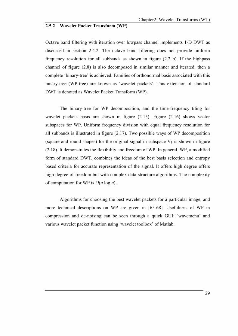
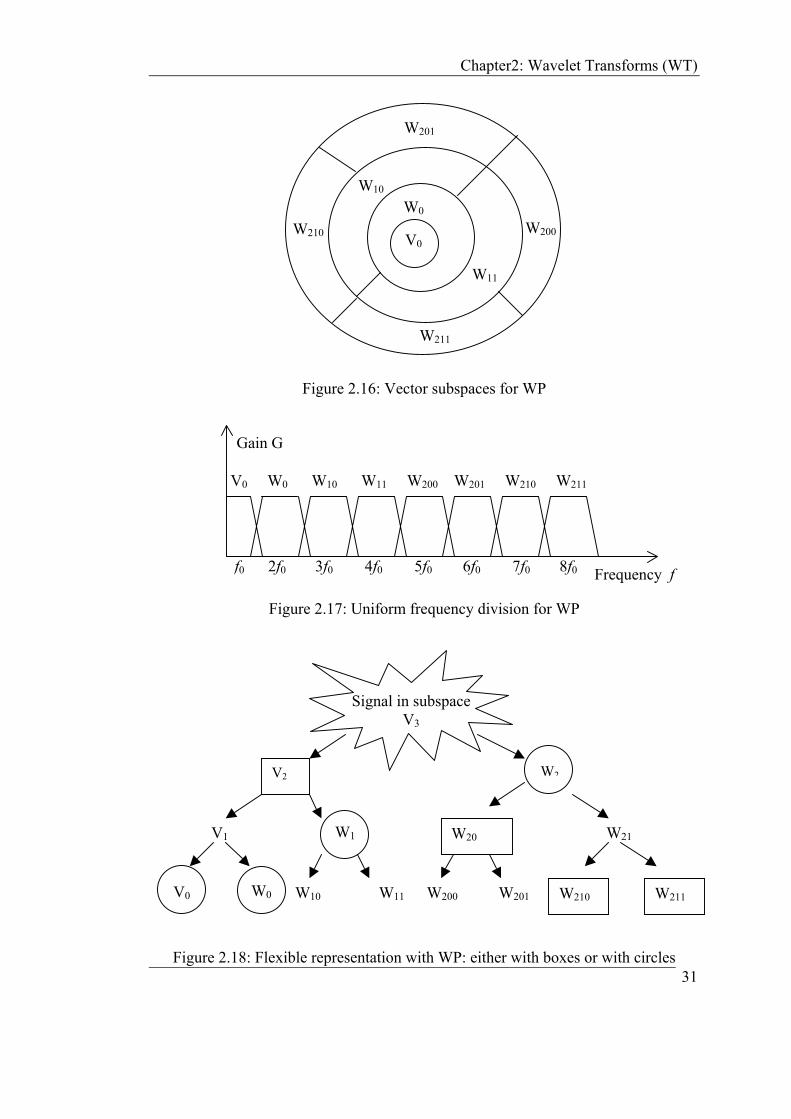
Chapter2: Wavelet Transforms (WT) 2.5.2 Wavelet Packet Transform (WP)
Octave band filtering with iteration over lowpass channel implements 1-D DWT as
discussed in section 2.4.2. The octave band filtering does not provide uniform
frequency resolution for all subbands as shown in figure (2.2 b). If the highpass
channel of figure (2.8) is also decomposed in similar manner and iterated, then a
complete ‘binary-tree’ is achieved. Families of orthonormal basis associated with this
binary-tree (WP-tree) are known as ‘wavelet packets’. This extension of standard
DWT is denoted as Wavelet Packet Transform (WP).
The binary-tree for WP decomposition, and the time-frequency tiling for
wavelet packets basis are shown in figure (2.15). Figure (2.16) shows vector
subspaces for WP. Uniform frequency division with equal frequency resolution for
all subbands is illustrated in figure (2.17). Two possible ways of WP decomposition
(square and round shapes) for the original signal in subspace V3 is shown in figure
(2.18). It demonstrates the flexibility and freedom of WP. In general, WP, a modified
form of standard DWT, combines the ideas of the best basis selection and entropy
based criteria for accurate representation of the signal. It offers high degree offers
high degree of freedom but with complex data-structure algorithms. The complexity
of computation for WP is O(n log n).
Algorithms for choosing the best wavelet packets for a particular image, and
more technical descriptions on WP are given in [65-68]. Usefulness of WP in
compression and de-noising can be seen through a quick GUI: ‘wavemenu’ and
various wavelet packet function using ‘wavelet toolbox’ of Matlab.
29

Chapter2: Wavelet Transforms (WT)
(a)
(b)
W21
W20
W1
V1
V2
W2
V3
↓2
↓2
↓2
↓2
↓2
↓2
↓2
↓2
h1
h0
h1
h0
h1
h0
h0
h1
↓2
↓2
↓2
↓2h1
h0
h1
h0
↓2 h1
↓2 h0
f
t
Equal bandwidth ∆f for all subbands
V0
W0
W10
W11
W200
W201
W210
W211
30
Figure 2.15: Wavelet packet transform:(a) binary-tree decomposition, (b) time-
frequency tiling of basis
Chapter2: Wavelet Transforms (WT)
W11
W210
W211
W201
W200
W0
V0
W10
Figure 2.16: Vector subspaces for WP
f0 2f0 3f0 4f0 5f0 6f0 7f0 8f0
Gain G
Frequency f
V0 W0 W10 W11 W200 W201 W210 W211
Figure 2.17: Uniform frequency division for WP
W1
V 0
W211 W210 W11 W200 W201 W10
W21 W20 V1
V2
Signal in subspace V3
2W
W 0
31Figure 2.18: Flexible representation with WP: either with boxes or with circles

Chapter2: Wavelet Transforms (WT) 2.5.3 Stationary Wavelet Transform (SWT)
The standard DWT as discussed in section 2.4.2 is a non-redundant and compact
representation of signal in transform domain. The decimation step after filtering
makes the standard DWT time shift-variant. The stationary wavelet transform (SWT)
has a similar tree structured implementation without any decimation (sub-sampling)
step. The balance for PR is preserved through level dependent zero-padding
interpolation of respective lowpass and high pass filters in the filter bank structures.
DWT of such kind is based on the ‘A Trous’ algorithm, which modifies the filters
through insertion of holes [69].
In literature, various interpretations of SWT are referred to as redundant, non-
decimated, overcomplete or shift-invariant wavelet transform. The implementation
structure for SWT is shown in figure (2.19), where * denotes the discrete time
convolution, di are detail (wavelet) coefficients and ci are approximate (scaling)
coefficients generated through the convolution chain originated from an original
signal sequence c0 and level-adaptive size-varying highpass filter h1 and lowpass
filter h0 respectively.
c0
c3c2c1
d1
h1
h0
22
∗ ∗ ∗
2
∗ ∗
2
∗
d2 d3
Figure 2.19: Three level decomposition with SWT
32

Chapter2: Wavelet Transforms (WT) SWT has equal length wavelet coefficients at each level. The computational
complexity of SWT is Ο (n2). The redundant representation makes SWT shift-
invariant and suitable for applications such as edge detection, denoising and data
fusion. The wavelet toolbox function ‘swt’ is the Matlab implementation of the same
algorithm.
2.6 Applications of Wavelet Transforms
Finally, applications of widely used standard DWT implementations, utilizing its
Multiscale and Multiresolution capabilities with fast filterbank algorithms are
numerous to describe. Depending upon the application, extensions of standard DWT
namely WP and SWT are also employed for improved performance at the cost of
higher redundancy and computational complexity.
A few of such applications in Data compression, Denoising, Source and
channel coding, Biomedical, Non-destructive evaluation, Numerical solutions of
PDE, Study of distant universe, Zero-crossings, Fractals, Turbulence, and Finance
etc. are comprehensively covered in [13]. Wavelet applications in many diverse
fields such as Physics, Medicine and biology, Computer Graphics, Communications
and multimedia etc. can be found in various books on wavelets [70-74].
2.7 Limitations of Wavelet Transforms Although the standard DWT is a powerful tool, it has three major disadvantages that
undermines its application for certain signal and image processing tasks [75]. These
disadvantages are described as below.
1. Shift Sensitivity:
A transform is shift sensitive, if the shifting in time, for input-signal causes an
unpredictable change in transform coefficients. It has been observed that the standard
DWT is seriously disadvantaged by the shift sensitivity that arises from down
samplers in the DWT implementation [14,76]. Shift sensitivity is an undesirable
property because it implies that DWT coefficients fail to distinguish between input-
33

Chapter2: Wavelet Transforms (WT) signal shifts. The shift variant nature of DWT is demonstrated with three shifted
step-inputs in figure (2.20). In figure (2.20) input shifted signals are decomposed up
to J= 4 levels using ‘db5’. It shows the unpredictable variations in the reconstructed
detail signal at various levels and in final approximation. Wavelet packets have also
been investigated for shift sensitivity. WP gives better results than standard DWT
implementation at the cost of complexity. The selection of best bases and cycle
spinning reduces shift sensitivity, but a general representation of WP is not shift
invariant [31,77]. Though SWT is shift invariant, it has a very large redundancy and
increased computational complexity.
Figure 2.20: Shift-sensitivity of standard 1-D DWT
2. Poor Directionality:
An m- Dimensional transform (m>1) suffers poor directionality when the transform
coefficients reveal only a few feature orientations in the spatial domain. As discussed
in section 2.5.1, the separable 2-D DWT partitions the frequency domain into three
directional subbands.
34

Chapter2: Wavelet Transforms (WT) As shown in figures (2.14 b) and (2.21), 2-D DWT can resolve only three
spatial-domain feature orientations: horizontal (HL), vertical (LH) and diagonal
(HH). Natural images contain number of smooth regions and edges with random
orientations; hence poor directionality affects the optimal representation of natural
images with of the separable standard 2-D DWT.
LH HL HH
Figure 2.21: Directionality of standard 2D DWT
Implementations of 2-D WP explore all frequency bands, and it can be
tailored for the selection of the best pattern (basis). However, the Multiscale structure
of wavelet decomposition and the concept of ‘spatial orientation tree’ [78] are lost. 2-
D form of WP is investigated for directionality in texture analysis applications
[79,80]. When compared with the standard 2-D DWT, because of its richer set of
basis, WP perform better in terms of fidelity of direction but not in terms of
improved directionality. The SWT is based on a filterbank structure, identical to
standard DWT as far as directionality is concerned, and hence SWT has poor
directionality. But SWT has improved fidelity in available direction because of large
redundancy.
3. Absence of Phase Information:
For a complex valued signal or vector, its phase can be computed by its real and
imaginary projections. Digital image is a data matrix with a finite support in 2-D.
Filtering the image with 2-D DWT increases its size and adds phase distortion.
Human visual system is sensitive to phase distortion [81]. Further more, ‘Linear
phase’ filtering can use symmetric extension methods to avoid the problem of
35
Chapter2: Wavelet Transforms (WT) increased data size in image processing [81]. Phase information is valuable in many
signal processing applications [83] such as e.g. in image compression and power
measurement [84,85].
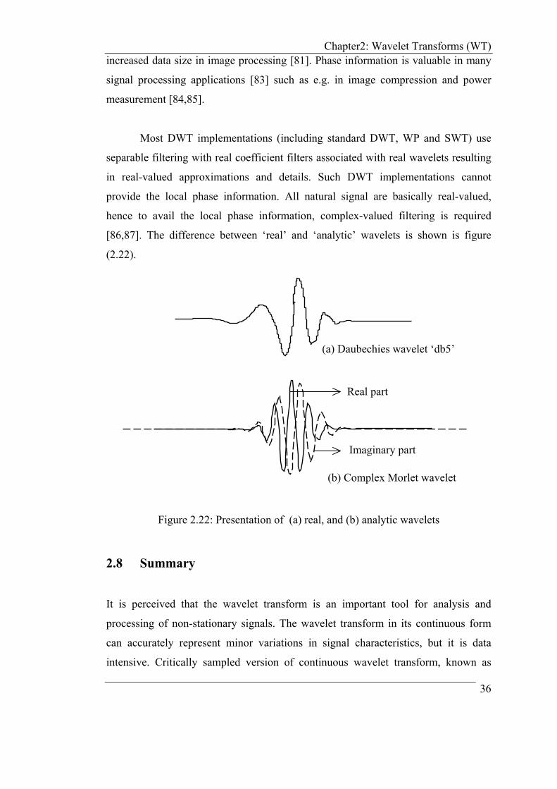
Most DWT implementations (including standard DWT, WP and SWT) use
separable filtering with real coefficient filters associated with real wavelets resulting
in real-valued approximations and details. Such DWT implementations cannot
provide the local phase information. All natural signal are basically real-valued,
hence to avail the local phase information, complex-valued filtering is required
[86,87]. The difference between ‘real’ and ‘analytic’ wavelets is shown is figure
(2.22).
(a) Daubechies wavelet ‘db5’
(b) Complex Morlet wavelet
Imaginary part
Real part
Figure 2.22: Presentation of (a) real, and (b) analytic wavelets
2.8 Summary
It is perceived that the wavelet transform is an important tool for analysis and
processing of non-stationary signals. The wavelet transform in its continuous form
can accurately represent minor variations in signal characteristics, but it is data
intensive. Critically sampled version of continuous wavelet transform, known as
36

Chapter2: Wavelet Transforms (WT) standard DWT, is very popular for denoising and compression in a number of
applications by the virtue of its computational simplicity through fast filterbank
algorithms, and non-redundancy. Though there are certain signal processing
applications (e.g. Edge detection, Time-division multiplexing in
Telecommunication), where more optimal representation is achieved through
redundant and computationally intensive extensions of standard DWT such as WP
and SWT.
All these forms of DWTs result in real valued transform coefficients with two
or more limitations as discussed in section 2.7. There is an alternate way of reducing
these limitations with a limited redundant representation in complex domain.
Formulation of complex-valued ‘analytic∗ filters’ or ‘analytic wavelets’ helps to get
the required phase information, more orientations, and reduced shift-sensitivity.
Various approaches of filterbank implementation employing analytic filters
associated with analytic wavelets are commonly referred to as ‘Complex Wavelet
Transforms’ (CWT). The formulations of analytic filter and associated complex
wavelet transforms are discussed in chapter 3.
∗ An ‘Analytic function’ is a complex valued function, constructed form a given real-valued
function by its projections on real and imaginary subspaces (Hilbert space). These projections are
termed as ‘Hardy space’ projections. The important property of an analytic signal is that its FT has
single-sided spectral components [2,88,89].
37
Chapter 3: Complex Wavelet Transforms (CWT)
Chapter 3:
Complex Wavelet Transforms (CWT)
3.1 Introduction
It is discussed in section 2.7 that standard DWT and its extensions suffer from two or
more serious limitations. The initial motivation behind the earlier development of
complex-valued DWT was the third limitation that is the ‘absence of phase
information’ [86]. Complex Wavelets Transforms (CWT) use complex-valued
filtering (analytic filter) that decomposes the real/complex signals into real and
imaginary parts in transform domain. The real and imaginary coefficients are used to
compute amplitude and phase information, just the type of information needed to
accurately describe the energy localisation of oscillating functions (wavelet basis).
Edges and other singularities in signal processing applications manifest themselves
as oscillating coefficients in the wavelet domain. The amplitude of these coefficients
describes the strength of the singularity while the phase indicates the location of
singularity. In order to determine the correct value of localised envelope and phase of
an oscillating function, ‘analytic’ or ‘quadrature’ representation of the signal is used.
This representation can be obtained from the Hilbert transform of the signal as
described in section 3.4 [88,89]. It is shown in [90] that for radar and sonar
applications, the complex I/Q orthogonal signals can be efficiently processed with
complex filterbanks rather than processing the I and Q channel separately. Thus, the
38

Chapter 3: Complex Wavelet Transforms (CWT)
complex orthogonal wavelet may prove to be a good choice, since it will allow
processing of both magnitude and phase simultaneously.
Chapter 3 is organised into eight sections. An introduction to complex wavelet
transforms is given in section 3.1. A review of earlier work and the recent
developments in the field of complex wavelet transforms are given in section 3.2 and
in section 3.3 respectively. Formal definition and mathematical formulation of
‘analytic filter’ is described in section 3.4, which is central to the design of all recent
complex wavelet transforms (CWT). In section 3.5, Dual-Tree DWT (DT-DWT)
forms of Redundant Complex Wavelet Transforms (RCWT) are discussed. The
filterbank structure, design methods and typical properties of DT-DWTs are also
described in section 3.5. Section 3.6 describes the basic design concept of complex
projection (mapping) based Non-Redundant CWT (NRCWT) and their properties.
All forms of CWTs are comprehensively compared in section 3.7, their advantages
and applications over standard DWT are also presented. Section 3.8 is a summary of
the investigations on CWTs.
3.2 Earlier Work
There is no one unique extension of the standard DWT into the complex plane.
Lawton [86], and Lina [91], showed that complex solutions of Daubechies wavelets
are possible. The complex valued Symmetric Daubechies Wavelets (SDW) has been
used for applications such as image enhancement, restoration and coding
[86,87,91,92]. The filterbank design to generate complex wavelets with useful
properties of orthogonality, symmetry and linear phase is described by Zang et. al.
[90].
The orthogonality is necessary to preserve the energy in transform domain.
The symmetry property of filter makes it easy to handle the boundary problem for
finite length signals [14]. Linear phase response of the filter is necessary, to reduce
the visually objectionable artifacts caused by nonlinear phase distortion, for the
quality of image [32]. All these complex solutions [86,87,90] result in orthogonal, 39

Chapter 3: Complex Wavelet Transforms (CWT)
symmetric, linear phase filter pairs, resulting in a combination of beneficial
properties that cannot be obtained with real-valued filter bank.
However, the impulse responses of the filters of all such complex solutions
lack the quadrature (Hilbert pair) between their real and imaginary parts, a desirable
property for the correct interpretation of local phase of the signal. As the Hilbert
transform is global in nature (infinitely extended in both time/frequency domain), it
is not directly applicable to localised wavelets with compact support. This
observation points to the need for the design of local filters with properties similar to
the Hilbert transform. The recent research in the field of CWT is directed towards the
design of complex valued filter bank structure such that the resulting wavelets (real
and imaginary parts) after high pass filtering form the (approximately) Hilbert
transform pairs at each successive level in the framework of standard DWT
decomposition structure (as described in section 2.4.2) [93-100].
3.3 Recent Developments
Recent research in the development of CWTs can be broadly classified in two
groups; RCWT (Redundant CWTs) and NRCWT (Non-redundant CWTs) as shown
in table (3.1). Standard DWT is critically decimated and gives N samples in
transform domain for the same N samples of a given signal. While the redundant
transform gives M samples in transform domain for N samples of given input signal
(where M>N) and hence it is expensive by the factor M/N. The NRCWT follows the
design aim to approach towards N samples in transform domain for a given N input
samples [101-105].
The RCWT include two almost similar CWTs. They are denoted as DT-DWT
(Dual-Tree DWT based CWT) with two almost similar versions namely Kingsbury’s
DT-DWT(K), and Selesnick’s DT-DWT(S) as classified in table (3.1). These
redundant transforms consist of two conventional DWT filterbank trees working in
parallel with respective filters of both the trees in approximate quadrature. The
filterbank structure of both DT-DWTs (as described in section 3.5.2) is same but the 40

Chapter 3: Complex Wavelet Transforms (CWT)
design methods to generate the filter coefficients are different. Both DT-DWTs
provide phase information; they are shift-invariant with improved directionality
[94,98-99]. Selesnick [98,99] proposed an alternative filter design methods for DT-
DWT(K) and designed DT-DWT(S), almost equivalent to DT-DWT(K) such that in
the limit the scaling and wavelet functions form Hilbert transform pairs. DT-DWT(S)
is designed with simple methods to obtain filter coefficients.
Selesnick’s DDTWT (Double Density Dual-Tree DWT) [108] is the initial
and more redundant version of DT-DWT(S). DDTWT can be viewed as the
combination of DDWT (Double Density DWT) [107] and DT-DWT(K). DDTWT
again consists of two DDWT (Double Density DWT) trees working in parallel with
respective filters in both trees are in approximate quadrature. Though the dual-tree
DWT based CWT reduce all three disadvantages of standard DWT, the redundancy
(though limited) of the transform is a drawback for applications like compression.
To remove this disadvantage, Spaendonck et. al. [104] created a set of
projection-based non-redundant complex wavelet transforms (NRCWT). The
projection (mapping) means converting a real signal to analytic (complex) form
through digital filtering. NRCWT is the DWT of that complex valued projection.
While these transforms are restricted to IIR filters, Fernandes et. al. [105] showed
that they produce orthogonal solutions. Fernandes’s projection based CWT (PCWT)
use flexible design techniques to trade-off between redundancy and shift-invariance.
Spaendonck’s OHCWT (Orthogonal Hilbert transform filterbank based
CWT) [103] is a three-band orthonormal complex wavelet transform with no-
redundancy for both real- and complex- valued signals. The class of projection based
NRCWT suggest their potential benefit in compression. Various design approaches
to reduce one or more disadvantages of standard DWT are summarized in [75].
41
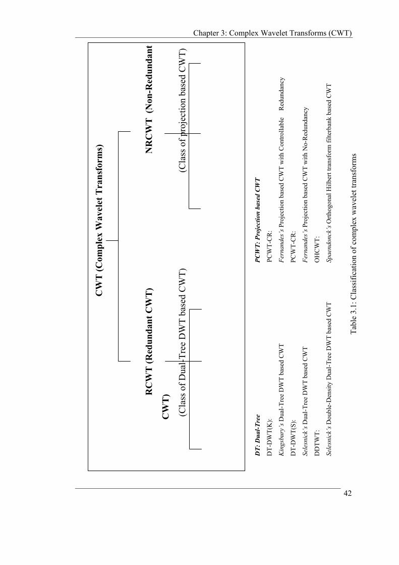
Chapter 3: Complex Wavelet Transforms (CWT)
DT:
Dua
l-Tre
e
PCW
T: P
roje
ctio
n ba
sed
CW
T
DT-
DW
T(K
):
P
CW
T-C
R:
Kin
gsbu
ry’s
Dua
l-Tre
e D
WT
base
d C
WT
Fe
rnan
des’
s Pro
ject
ion
base
d C
WT
with
Con
trolla
ble
R
edun
danc
y
DT-
DW
T(S)
:
PC
WT-
CR
:
Sele
snic
k’s D
ual-T
ree
DW
T ba
sed
CW
T
Fe
rnan
des’
s Pro
ject
ion
base
d C
WT
with
No-
Red
unda
ncy
DD
TWT:
O
HC
WT:
Sele
snic
k’s D
oubl
e-D
ensi
ty D
ual-T
ree
DW
T ba
sed
CW
T
Sp
aend
onck
’s O
rthog
onal
Hilb
ert t
rans
form
filte
rban
k ba
sed
CW
T
Tabl
e 3.
1: C
lass
ifica
tion
of c
ompl
ex w
avel
et tr
ansf
orm
s
CW
T (C
ompl
ex W
avel
et T
rans
form
s)
RC
WT
(Red
unda
nt C
WT
)
NR
CW
T (
Non
-Red
unda
nt
CW
T)
(Cla
ss o
f Dua
l-Tre
e D
WT
base
d C
WT)
(Cla
ss o
f pro
ject
ion
base
d C
WT)
42
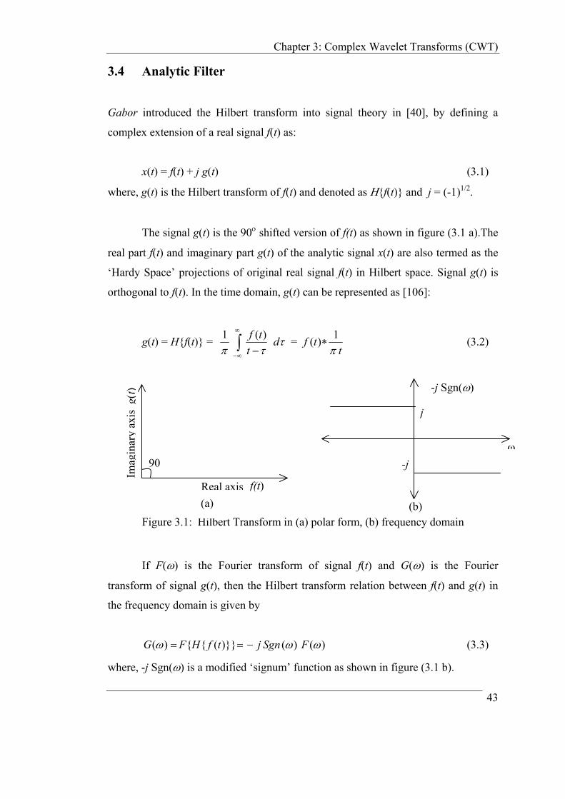
Chapter 3: Complex Wavelet Transforms (CWT)
3.4 Analytic Filter
Gabor introduced the Hilbert transform into signal theory in [40], by defining a
complex extension of a real signal f(t) as:
x(t) = f(t) + j g(t) (3.1)
where, g(t) is the Hilbert transform of f(t) and denoted as Η{f(t)} and j = (-1)1/2.
The signal g(t) is the 90ο shifted version of f(t) as shown in figure (3.1 a).The
real part f(t) and imaginary part g(t) of the analytic signal x(t) are also termed as the
‘Hardy Space’ projections of original real signal f(t) in Hilbert space. Signal g(t) is
orthogonal to f(t). In the time domain, g(t) can be represented as [106]:
g(t) = H{f(t)} = ττπ
dt
tf∫∞
∞− −)(1 =
ttf
π1)( ∗ (3.2)
Figure 3.1: Hilbert Transform in (a) polar form, (b) frequency domain
90
f(t) Real axis
Imag
inar
y ax
is g
(t)
(a)
ω
j
-j
(b)
-j Sgn(ω)
If F(ω) is the Fourier transform of signal f(t) and G(ω) is the Fourier
transform of signal g(t), then the Hilbert transform relation between f(t) and g(t) in
the frequency domain is given by
)()()}}({{)( ωωω FSgnjtfHFG −== (3.3)
where, -j Sgn(ω) is a modified ‘signum’ function as shown in figure (3.1 b).
43

Chapter 3: Complex Wavelet Transforms (CWT)
This analytic extension provides the estimate of instantaneous frequency and
amplitude of the given signal x(t) as:
Magnitude of x(t) = ))()(( 22 tgtf +
Angle of x(t) = tan-1[ g(t)/ f(t) ] (3.4)
The other unique benefit of this quadrature representation is the non-negative
spectral representation in Fourier domain [89,106], which leads toward half the
bandwidth utilisation. The reduced bandwidth consumption is helpful to avoid
aliasing of filter bands especially in multirate signal processing applications. The
reduced aliasing of filter bands is the key for shift-invariant property of CWT. The
single-sided spectral representation of an analytic signal is illustrated in figure (3.2).
(a) ω ω
X(ω) F(ω)
(b)
12
Figure 3.2: Spectral representation of (a) original signal f(t), (b) analytic signal x(t)
The same concept of analytic or quadrature formulation is applied to the
filterbank structure of standard DWT to produce complex solutions and in turn the
CWT. The real-valued filter coefficients are replaced by complex-valued coefficients
by proper design methodology that satisfies the required conditions for convergence.
Then the complex filter can again be decomposed into two real-valued filters. Thus,
two real-valued filters that give their respective impulse responses in quadrature will
form the Hilbert transform pair. The combined pair of two such filters is termed as an
analytic filter. The formulation and interpretation of the analytic filter is shown in
figure (3.3).
44
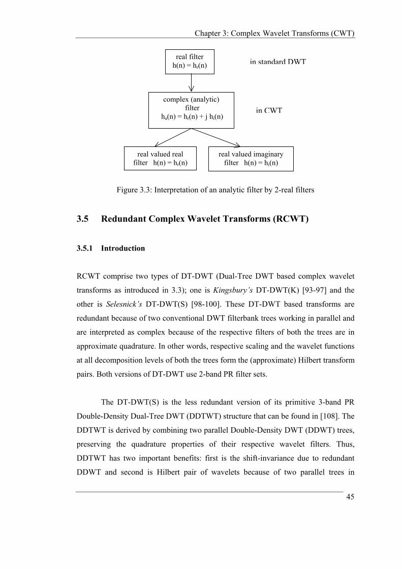
Chapter 3: Complex Wavelet Transforms (CWT)
real valued real filter h(n) = hr(n)
real valued imaginary filter h(n) = hi(n)
real filter h(n) = hr(n)
complex (analytic) filter
ha(n) = hr(n) + j hi(n)
in standard DWT
in CWT
Figure 3.3: Interpretation of an analytic filter by 2-real filters
3.5 Redundant Complex Wavelet Transforms (RCWT)
3.5.1 Introduction
RCWT comprise two types of DT-DWT (Dual-Tree DWT based complex wavelet
transforms as introduced in 3.3); one is Kingsbury’s DT-DWT(K) [93-97] and the
other is Selesnick’s DT-DWT(S) [98-100]. These DT-DWT based transforms are
redundant because of two conventional DWT filterbank trees working in parallel and
are interpreted as complex because of the respective filters of both the trees are in
approximate quadrature. In other words, respective scaling and the wavelet functions
at all decomposition levels of both the trees form the (approximate) Hilbert transform
pairs. Both versions of DT-DWT use 2-band PR filter sets.
The DT-DWT(S) is the less redundant version of its primitive 3-band PR
Double-Density Dual-Tree DWT (DDTWT) structure that can be found in [108]. The
DDTWT is derived by combining two parallel Double-Density DWT (DDWT) trees,
preserving the quadrature properties of their respective wavelet filters. Thus,
DDTWT has two important benefits: first is the shift-invariance due to redundant
DDWT and second is Hilbert pair of wavelets because of two parallel trees in
45

Chapter 3: Complex Wavelet Transforms (CWT)
quadrature. It is important to note that DDWT is a shift invariant 3-band redundant
DWT but not a CWT [107].
Both DT-DWTs have same filterbank structure, which is described in 3.5.2.
The DT-DWTs use the analysis and synthesis filterbank structures (figure (3.4)) that
seem identical to those used for standard DWT as shown in figures (2.8) and (2.9).
The key difference is that all the real filters are replaced with analytic filters
formulated in figure (3.3) to have complex solutions. The replacement of real filters
with analytic filters makes the new structure equivalent to two standard DWT
filterbank structures operating in parallel. Because of two parallel trees for analysis
as well as synthesis, these CWT are described as Dual-Tree DWT based CWT. The
insertion of the parallel structure eliminates the disadvantages of standard DWT but
makes it redundant (limited) and expensive for applications like signal compression.
3.5.2 Filterbank Structure of Dual-Tree DWT based CWT
The filterbank structures for both DT-DWTs are identical. Figure (3.4) shows 1-D
analysis and synthesis filterbanks spanned over three levels. It is evident from the
filterbank structure of DT-DWT that it resembles the filterbank structure of standard
DWT with twice the complexity. It can be seen as two standard DWT trees operating
in parallel. One tree is called as a real tree and other is called as an imaginary tree.
Sometimes in future discussions the real tree will be referred to as tree-a and the
imaginary tree as tree-b.
The form of conjugate filters used in 1-D DT-DWT is given as:
(hx + j gx)
where, hx is the set of filters {h0, h1}, and gx is the set of filters {g0, g1} both sets in
only x-direction (1-D).
The filters h0 and h1 are the real-valued lowpass and highpass filters respectively for
real tree. The same is true for g0 and g1 for imaginary tree.
46
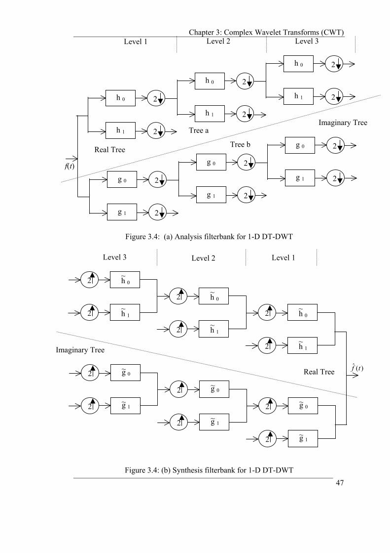
Chapter 3: Complex Wavelet Transforms (CWT)
Level 1 Level 2 Level 3
h 1
h 0 2
2
h 1
h 0 2
2
h 1
h 0 2
2
g 1
g 0 2
2
g 1
g 0 2
2
g 1
g 0 2
2
Real Tree
Imaginary Tree
f(t)
Tree a
Tree b
Figure 3.4: (a) Analysis filterbank for 1-D DT-DWT
h~ 0 2
2
h~ 1
h~ 0 2
2
h~ 1
h~ 0 2
2
g~ 1
g~ 0 2
2
g~ 1
g~ 0 2
2
g~ 1
g~ 0 2
2
)(ˆ tf
Level 3 Level 2 Level 1
Real Tree
Imaginary Tree
h~ 1
Figure 3.4: (b) Synthesis filterbank for 1-D DT-DWT
47

Chapter 3: Complex Wavelet Transforms (CWT)
Though the notation of h0 and h1 are use for all level in the real part of analysis tree,
h0 and h1 of first level are numerically different then the respective filters at all other
levels above level-1. The reason for such difference will be discussed later in the
filter designs for both the DT-DWTs separately. The same notion is applied for
imaginary tree filters g0 and g1. The synthesis filter pairs 10~,~ hh , and 1,0
~~ gg as shown
in figure (3.4 b) form orthogonal or biorthogonal pairs with their respective
counterpart filters of analysis tree as shown in figure (3.4 a).
The 2-D DT-DWT structure has an extension of conjugate filtering in 2-D
case. The filterbank structure of 2-D dual-tree is shown in figure (3.5). 2-D structure
needs four trees for analysis as well as for synthesis. The pairs of conjugate filters are
applied to two dimensions (x and y), which can be expressed as:
(hx + j gx) (hy + j gy) = (hxhy - gxgy) + j (hxgy + gxhy) (3.5)
Tree a (hx hy)
Tree b (gx gy)
Tree c (hx gy)
Tree d (gx hy)
Tree a~ ( yh~h~x )
Tree b~ ( ygxg~ )
Tree c~ ( yg~h~x )
Tree d~ ( yh~g~x )
Real Trees
Imaginary Trees
(t) )(~ tf
Analysis Synthesis
f
Figure 3.5: Filterbank structure for 2-D DT-DWT
48

Chapter 3: Complex Wavelet Transforms (CWT)
The filterbank structure of tree-a, similar to standard 2-D DWT spanned over
3-level, is shown in figure (3.6). All other trees-(b,c,d) have similar structures with
the appropriate combinations of filters for row- and column- filtering. The overall 2-
D dual-tree structure is 4-times redundant (expensive) than the standard 2-D DWT.
The tree-a and tree-b form the real pair, while the tree-c and tree-d form the
imaginary pair of the analysis filterbank. Trees-( ba ~,~ ) and trees-( dc ~,~ ) are the real
and imaginary pairs respectively in the synthesis filterbank similar to their
corresponding analysis pairs.
hx0
hx1
hy0
hy1
hy0
hy1
hx0
hx1
hy0
hy1
hy0
hy1
hx0
hx1
hy0
hy1
hy0
hy1
Level 1 Level 2 Level 3
Figure 3.6: Filterbank structure of tree-a of figure 3.5
3.5.3 Kingsbury’s Dual-Tree DWT (DT-DWT(K))
It is observed that approximate shift invariance is possible with standard DWT (i.e.
tree-a) by doubling the sampling rate at each level of the tree [95]. For this to work,
the samples must be evenly spaced and down samplers must be eliminated after the
level-1 filters. This is equivalent to having two parallel fully decimated trees, real
(tree-a) and imaginary (tree-b) as in figure (3.4) if the delays of first level filters of
tree-b are one sample offset by their corresponding filter in tree-a. 49

Chapter 3: Complex Wavelet Transforms (CWT) Level 1 Level 2 Level 3
h 1a
h 0a 2
2
h 01a
h 00a 2
2
h 001a
h 000a 2
2
g 1b
g 0b 2
2
g 01b
g 00b 2
2
g 001b
g 000b 2
2
Real Tree
Imaginary Tree
f(t)
Tree a Tree b
odd
odd
even
even
odd
odd
½ sample delay
½ sample delay
1 sample delay
Figure 3.7: Analysis tree using odd-even filters
50
odd
odd
even
even
even
½ sample delay
½ sample delay
1 sample delay even
Level 1 Level 2 Level 3
h 000a (3q) 2
h 00a(3q) 2
h 001a (q) h(1) 0a 2 2
h 01a(q) 2
Imaginary Tree h(0) 1a Tree a 2
b (q) Tree b g 000 2 Real Tree
g 00b(q) 2 f(t)
g 001b (3q) g(0) 0b 2 2
1b(3q)g 0 2
g(1) 1b 2
Figure 3.8: Analysis tree using Q-shift filters. Figure in brackets inside a filter block indicates the delay for each filter, where q = ¼ samples

Chapter 3: Complex Wavelet Transforms (CWT)
This offset ensures the pickup of opposite samples in both trees. To get uniform
interval between the samples of both trees after level-1, filters in one tree must
provide delays that are half a sample different from those in opposite tree.
The DT-DWT(K) can be designed in two ways to have required delays. The
first is based on odd-even length filters and the second employs Q-shift (quarter
shift) filter design. The filterbank structures of analysis tree with odd-even filters and
Q-shift filters are shown in figures (3.7) and (3.8) respectively. The key issue in the
design of DT-DWT(K) is to obtain (approximate) shift invariance using any of the
filter forms.
Constraints for Shift Invariance:
To check the shift invariance, only one type of coefficients (either scaling or
wavelet) of both the trees at any one level is retained and all other coefficients at all
other levels are set to zero. If the reconstructed signal )(~ tf from these coefficients is
free of aliasing and follows the PR then the transform is said to be shift-invariant at
that level.
DT-DWT(K) structure (same as shown in figure 3.4) can be modelled as
shown in figure (3.9) using either odd-even (figure 3.7), or Q-shift (figure 3.8) filter
types.
Analysis Synthesis
M
M
M
C(Z)
D(Z)
Tree a
Tree b
)(~ ZF
)(~ ZFa
)(~ ZFb
)(ZF
M
B(Z)
A(Z)
Figure 3.9: Modelling of DT-DWT(K) filter structure for deriving the shift-invariance constraints
51

Chapter 3: Complex Wavelet Transforms (CWT)
The PR condition for DT-DWT(K) model (shown in figure (3.9)), using standard
multirate identities of [14] is given as:
)()(~)(~)(~ ZFZFZFZF ba =+=
= [ ])()()()()(1 1
0ZDZWBZCZWAZWX
Mkk
M
k
k +∑−
=
(3.6)
where, M = 2m is the total up/down sampling factor determined by the number of
levels (m) of the dual-tree. The factor W = Mj π2
e . Letters A, B represent transfer
functions of the analysis dual-tree and C, D represent the corresponding transfer
functions for the synthesis dual-tree.
For the sake of simplicity (by taking m =3), and only the wavelet coefficients
of level-3 are chosen to derive the constraints of shift invariance of DT-DWT(K). In
this case the transfer function A(Z) (h0a to h001a) and B(Z) (g0b to g001b) as shown in
figure (3.7) are modelled as:
)()()()( 4001
2000 ZHZHZHZA aaa=
)()()()( 4001
2000 ZGZGZGZB bbb= (3.7)
Similarly, C(Z) and D(Z) can be derived for synthesis tree.
The DT-DWT(K) can be shift-invariant if the aliasing terms
and of equation (3.6) are either very small or cancel
each other for k . The designing strategies, to reduce these aliasing terms for
approximate shift-invariance, are different for scaling (lowpass) and wavelet
(highpass) coefficients [95].
)()( ZCZWA k )()( ZDZWB k
0≠
For lowpass case aliasing can be reduced by letting:
52

Chapter 3: Complex Wavelet Transforms (CWT)
)()( 2 ZAzZBM
±= and )()( 2 ZCzZD
Mm
= so that
)()( ZDZWB k = (-1)k )()( ZCZWA k , for odd values of k. (3.8)
For highpass (bandpass) case, aliasing is generated by overlap of opposite
frequency pass bands in a single wavelet tree, where as wanted terms (k = 0) are
produced by overlap of same frequency pass bands. The solution is to give B and D
the upper and lower passbands of opposite polarity while A and C have the
passbands of the same polarity (or vice versa). The need to discriminate in this way
suggests the use of complex filters. Suppose P(Z) and Q(Z) are the prototype
complex filters, each with just a single sided passband, and let
[ ] )()()(2)( * ZPZPZPZA +=ℜ=
[ ] )]()([)(2)( * ZPZPjZPZB −−=ℑ=
[ ] )()()(2)( * ZQZQZQZC +=ℜ=
[ ] )]()([)(2)( * ZQZQjZQZD −=ℑ−= (3.9)
where [] and [] take real and imaginary parts, and conjugation of is given
by .
ℜ
)(Z
ℑ )(ZP*P
Hence P and Q are filters corresponding to the upper passbands of A and C
while *P and correspond to their lower passbands. This also applies to filters B
and D, except that their lower passbands are negated. The (real) impulse responses of
B and D are the Hilbert transforms of those of A and C. The portion of equation (3.6)
can be written as:
*Q
)()()()( ZDZWBZCZWA kk + = (3.10) )()(2)()(2 ** ZQZWPZQZWP kk +
The task of designing the filters such that the positive frequency complex
filter does not overlap with shifted versions of the similar filter becomes
easy due to their single sided spectral representation. The formulations in equation
)(ZQ )(ZP
53

Chapter 3: Complex Wavelet Transforms (CWT)
(3.9) show that the bandpass filter responses for trees-(a, b) (A, B for analysis; C, D
for reconstruction) should be regarded as the ‘real’ and ‘imaginary’ parts of complex
responses (P for analysis; Q for synthesis) that have passbands only on one side of
zero frequency. It is also possible to relate the pairs of scaling function coefficients
of both trees as real and imaginary parts.
The design of DT-DWT(K) is based on viewing the scaling coefficients from
tree-b as interpolating mid-way between the corresponding ones from tree-a. In
practice, the filters with compact support will not have zero gain in their stop bands
and the aliasing terms in equation (3.6) will not be zero. Furthermore, odd-length
filters cannot have precisely the same frequency responses as the even-length ones.
So a typical DT-DWT(K) will only be ‘approximately’ shift-invariant.
Odd-even length filters:
To have linear phase filters with required delay offset between filters beyond level-1
of both trees, it is necessary to have odd-length filters in one tree and even-length
filters in the other tree (figure 3.7). Greater symmetry between two trees can be
achieved if each tree uses odd and even filters alternately from level to level. The
filters at level-1 in both trees are odd length, and the corresponding lowpass and
highpass filter pairs are apart by one sample. The filters in synthesis tree may be
biorthogonal for PR or near-orthogonal for energy preservation (in transform
domain) to the filters of analysis tree. The odd-even filter design is based on
minimum mean squared error in the approximation. The coefficients of (13-19) tap
odd length and (12-16) even length filters can be found in [94,95].
Q-shift filters:
There are certain problems with odd-even length filter approach. First is that the sub-
sampling structure is not very symmetrical (wavelet and scaling functions at a given
scale are not well aligned). Second, the two trees have slightly different frequency
responses and the third problem is that filter sets must be biorthogonal, rather than
orthogonal, because they are linear phase.
54
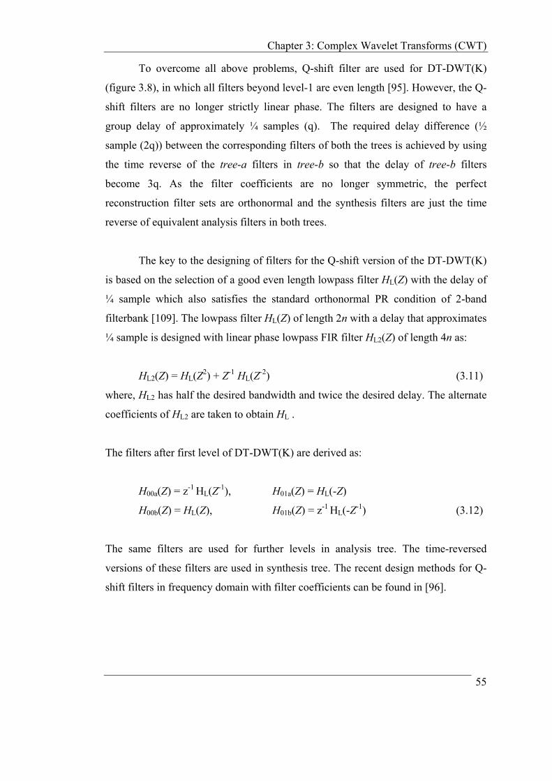
Chapter 3: Complex Wavelet Transforms (CWT)
To overcome all above problems, Q-shift filter are used for DT-DWT(K)
(figure 3.8), in which all filters beyond level-1 are even length [95]. However, the Q-
shift filters are no longer strictly linear phase. The filters are designed to have a
group delay of approximately ¼ samples (q). The required delay difference (½
sample (2q)) between the corresponding filters of both the trees is achieved by using
the time reverse of the tree-a filters in tree-b so that the delay of tree-b filters
become 3q. As the filter coefficients are no longer symmetric, the perfect
reconstruction filter sets are orthonormal and the synthesis filters are just the time
reverse of equivalent analysis filters in both trees.
The key to the designing of filters for the Q-shift version of the DT-DWT(K)
is based on the selection of a good even length lowpass filter HL(Z) with the delay of
¼ sample which also satisfies the standard orthonormal PR condition of 2-band
filterbank [109]. The lowpass filter HL(Z) of length 2n with a delay that approximates
¼ sample is designed with linear phase lowpass FIR filter HL2(Z) of length 4n as:
HL2(Z) = HL(Z2) + Z-1 HL(Z-2) (3.11)
where, HL2 has half the desired bandwidth and twice the desired delay. The alternate
coefficients of HL2 are taken to obtain HL .
The filters after first level of DT-DWT(K) are derived as:
H00a(Z) = z-1 HL(Z-1), H01a(Z) = HL(-Z)
H00b(Z) = HL(Z), H01b(Z) = z-1 HL(-Z-1) (3.12)
The same filters are used for further levels in analysis tree. The time-reversed
versions of these filters are used in synthesis tree. The recent design methods for Q-
shift filters in frequency domain with filter coefficients can be found in [96].
55

Chapter 3: Complex Wavelet Transforms (CWT)
3.5.4 Selesnick’s Dual-Tree DWT (DT-DWT(S))
The DT-DWT(S) is again a DT-DWT form of redundant complex wavelet transform
having the 1-D filterbank structure shown in figure (3.4). DT-DWT(S), proposed by
Selesnick [98] is an alternate design approach to Kingsbury’s DT-DWT(K) discussed
in section 3.5.3.
In [98,99], the alternate way to design the quadrature wavelet pair with
specified length and vanishing moment multiplicity is shown. The DT-DWT(S)
employs either ‘Grobner bases’ or general ‘spectral factorization’ methods for the
design of analytic filters to have quadrature pair of wavelets in a dual-tree structure.
The design of Hilbert transform pairs of wavelet basis with general spectral
factorization using flat-delay allpass filters is simpler than the Grobner bases based
solutions. The design of DT-DWT(S) also proves that for two orthogonal wavelets to
form a Hilbert transform pair, the scaling filters of both trees should be offset by a
half sample. The design is based on the limit function defined by infinite product
formula rather than the concept of midway interpolation of two lowpass filters for
approximate shift invariance (as in the case of DT-DWT(K)). The underlying
constraints for the design of DT-DWT(S) are discussed here with key equations from
[99].
For the filterbank structure, shown in figure (3.4), let h0 and h1 represent CQF
(Conjugate Quadrature Filter) pair [53]. That is,
)1()1()( 0)1(
1 nhnh n −−= − (3.13)
and, in Z-transform domain
)1(1)(
2)1()()1()(
01
0000
ZH
zZH
ZHZH
ZHZH
−=
=−−+ (3.14)
56

Chapter 3: Complex Wavelet Transforms (CWT)
The filters g0 and g1 represent a second CQF pair.
For all these real-valued filters hi and gi of DT-DWT(S), the dilation and
wavelet equations give the scaling and wavelet functions for the real tree as:
).2()(2)(
)2()(2)(
1
0
ntnht
ntnht
hn
h
hn
h
−=
−=
∑
∑ψψ
ϕϕ (3.15)
The scaling function )(tgϕ and wavelet )(tgψ are defined similarly for the imaginary
tree.
As discussed in section 3.4, )(tgψ is the Hilbert transform of )(thψ , )(tgψ =
H{ )(thψ }, if
0,)(
0,)()(
<=
>−=
ωωψ
ωωψωψ
h
hg
j
j (3.16)
where, )(ωψ h and )(ωψ g are the Fourier transforms of the wavelets associated with
the highpass filters of real and imaginary parts of DT-DWT(S). Similarly, )(0 ωH =
DTFT{h0(n)}, )(0 ωG = DTFT{g0(n)}are the Fourier transforms of scaling filters h0
and g0 respectively.
If )(thψ and )(tgψ form Hilbert transform pair, then
)()( ωψωψ gh = and therefore )()( 00 ωω GH = (3.17)
That is, the two lowpass filters are related as:
)(0 ωG = )(0 ωH )(ωθje− (3.18)
It is derived using infinite-product formula in [98] that it is possible only when
57

Chapter 3: Complex Wavelet Transforms (CWT)
πωωωθ <= ,2
)( (3.19)
Equivalently, the digital filter g0(n) is a half-sample delayed version of h0(n),
g0(n) = h0(n-1/2) (3.20)
As a half-sample delay can not be implemented with FIR filter, the
approximate design of FIR filters h0(n) and g0(n) is employed with Grobner bases or
spectral factorization [98,99]. The filter coefficients for DT-DWT(S) can be found
from [110]. Orthogonal filter sets are used for DT-DWT(S). First level of analysis
filterbank of DT-DWT(S) employs a unique lowpass filter pair to produce one pair
of Hilbert wavelets at that level, and after first level, a second distinct pair of lowpass
filters is repeated for the rest of the structure to produce the pairs of Hilbert wavelets
at all subsequent levels of the DT-DWT(S). All the synthesis filters are the time-
reversed version of their corresponding analysis filters.
3.5.5 Properties of DT-DWT
Both DT-DWTs (Dual-Tree DWT based CWTs) have similar properties because of
their identical filterbank structures. The important properties for the comparison with
standard DWT are Shift-sensitivity, Directionality and Phase-information. The key
properties of DT-DWT(K) and DT-DWT(S) are [95,99]:
1. Shift Invariance:
DT-DWT has approximate shift-invariance, or in other words, improved
time-shift sensitivity in comparison with standard DWT. The reconstructed
details at various levels and approximation at the last level have almost
uniform shifts for the time-shifted unit step functions. This property is very
clear from figure (3.10) compared to figure (2.20). The property of shift
invariance makes the DT-DWT well suited for applications such as Motion
estimation [111], and Image fusion [112] at various resolution levels.
58
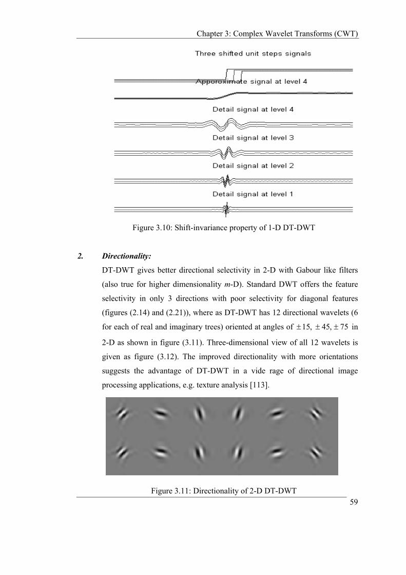
Chapter 3: Complex Wavelet Transforms (CWT)
Figure 3.10: Shift-invariance property of 1-D DT-DWT
2. Directionality:
DT-DWT gives better directional selectivity in 2-D with Gabour like filters
(also true for higher dimensionality m-D). Standard DWT offers the feature
selectivity in only 3 directions with poor selectivity for diagonal features
(figures (2.14) and (2.21)), where as DT-DWT has 12 directional wavelets (6
for each of real and imaginary trees) oriented at angles of in
2-D as shown in figure (3.11). Three-dimensional view of all 12 wavelets is
given as figure (3.12). The improved directionality with more orientations
suggests the advantage of DT-DWT in a vide rage of directional image
processing applications, e.g. texture analysis [113].
75,45,15 ±±±
Figure 3.11: Directionality of 2-D DT-DWT
59
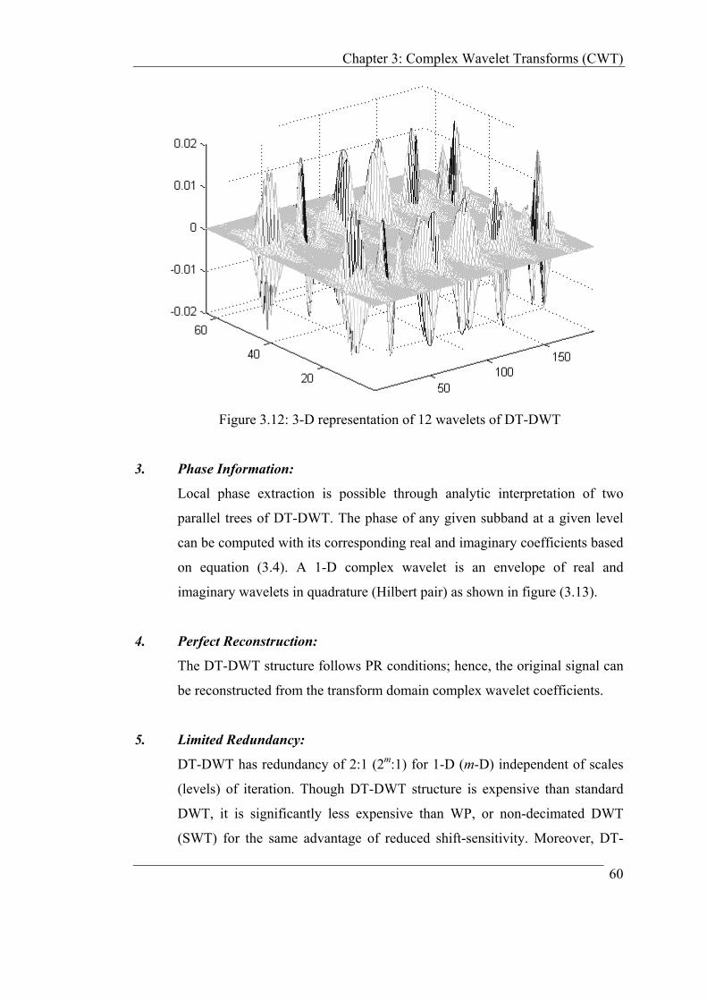
Chapter 3: Complex Wavelet Transforms (CWT)
Figure 3.12: 3-D representation of 12 wavelets of DT-DWT
3. Phase Information:
Local phase extraction is possible through analytic interpretation of two
parallel trees of DT-DWT. The phase of any given subband at a given level
can be computed with its corresponding real and imaginary coefficients based
on equation (3.4). A 1-D complex wavelet is an envelope of real and
imaginary wavelets in quadrature (Hilbert pair) as shown in figure (3.13).
4. Perfect Reconstruction:
The DT-DWT structure follows PR conditions; hence, the original signal can
be reconstructed from the transform domain complex wavelet coefficients.
5. Limited Redundancy:
DT-DWT has redundancy of 2:1 (2m:1) for 1-D (m-D) independent of scales
(levels) of iteration. Though DT-DWT structure is expensive than standard
DWT, it is significantly less expensive than WP, or non-decimated DWT
(SWT) for the same advantage of reduced shift-sensitivity. Moreover, DT-
60

Chapter 3: Complex Wavelet Transforms (CWT)
DWT has other advantages such as improved directionality and phase
information to compensate for its limited redundancy over standard DWT.
Figure 3.13: A complex wavelet as a quadrature combination of real and imaginary wavelets for 1-D DT-DWT
3.6 Non-Redundant Complex Wavelet Transforms (NRCWT)
3.6.1 Introduction
NRCWT is the class of complex projection (mapping) based DWT introduced in
section 3.3. NRCWT has two-stage implementation (figure 3.14); first is the complex
projection of a given signal and second is the implementation of any type of DWT on
that complex valued projection. The independence of two stages allows them to be
performed separately and alternatively leading towards a greater flexibility of
implementation.
61

Chapter 3: Complex Wavelet Transforms (CWT)
In true sense, all of the class of NRCWT are not exactly non-redundant CWT,
which are designed to mitigate all three disadvantages of standard DWT. These
complex wavelet transforms are categorized under NRCWT because of their two
broad design aims. First is to offer controllable redundancy that is equal or less than
the redundancy of DT-DWT (Dual-Tree based CWT or RCWT) while preserving all
the benefits similar to DT-DWT. Second aim is to offer improved directionality and
phase information with perfect non-redundancy at the cost of shift-invariant property
targeting mainly the signal compression applications.
Three types of NRCWT are listed in table (3.1). Fernandes’s PCWT-CR
(Projection based CWT with Controllable Redundancy) are the arbitrary DWT
implemented on redundant complex projection of the original signal to preserve all
potential benefits of DT-DWT. The PCWT-NR (Projection based CWT with No-
Redundancy) can be designed with perfectly no-redundancy using non-redundant
complex projection (mapping). PCWT-NR is directional but not shift-invariant. In
the same way Spaendonck’s OHCWT (Orthogonal Hilbert transform filterbank based
CWT) is a 3-band perfectly non-redundant and directional transform but is not shift-
invariant.
3.6.2 Projection based CWT (PCWT)
Fernandes et al. [75,105,114] introduced 2-stage projection (mapping) based CWT
that consist of mapping of a given real-world signal onto complex function space
through some digital filtering technique (will be discussed later) followed by any
type of DWT on the complex mapping.
3.6.2.1 Generic Structure
A generic implementation of projection based complex wavelet transform (PCWT) is
shown in figure (3.14). The forward CWT consists of an arbitrary DWT filterbank
preceded by a mapping stage (or vice versa). The reverse CWT has inverse mapping
stage after a synthesis DWT filterbank (or vice versa).
62
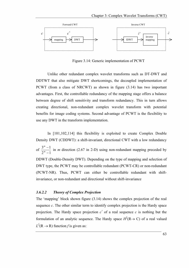
Chapter 3: Complex Wavelet Transforms (CWT)
Forward CWT Inverse CWT
63
Figure 3.14: Generic implementation of PCWT
Unlike other redundant complex wavelet transforms such as DT-DWT and
DDTWT that also mitigate DWT shortcomings, the decoupled implementation of
PCWT (from a class of NRCWT) as shown in figure (3.14) has two important
advantages. First, the controllable redundancy of the mapping stage offers a balance
between degree of shift sensitivity and transform redundancy. This in turn allows
creating directional, non-redundant complex wavelet transform with potential
benefits for image coding systems. Second advantage of PCWT is the flexibility to
use any DWT in the transform implementation.
In [101,102,114] this flexibility is exploited to create Complex Double
Density DWT (CDDWT): a shift-invariant, directional CWT with a low redundancy
of 1213
−−
m
m
in m direction (2.67 in 2-D) using non-redundant mapping preceded by
DDWT (Double-Density DWT). Depending on the type of mapping and selection of
DWT type, the PCWT may be controllable redundant (PCWT-CR) or non-redundant
(PCWT-NR). Thus, PCWT can either be controllable redundant with shift-
invariance, or non-redundant and directional without shift-invariance
3.6.2.2 Theory of Complex Projection
The ‘mapping’ block shown figure (3.14) shows the complex projection of the real
sequence c. The other similar term to identify complex projection is the Hardy space
projection. The Hardy space projection c+ of a real sequence c is nothing but the
formulation of an analytic sequence. The Hardy space H2(R→ C) of a real valued
L2(R → R) function f is given as:
mapping DWT
c+ +c c cinverse
IDWT mapping
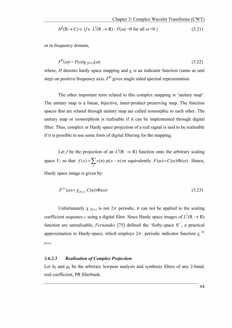
Chapter 3: Complex Wavelet Transforms (CWT)
H2(R→ C) ≡ {f ∈ L2(R → R) : F(ω) =0 for all ω <0 } (3.21)
or in frequency domain,
FH(ω) = F(ω)χ [0,∞)(ω) (3.22)
where, H denotes hardy space mapping and χ is an indicator function (same as unit
step) on positive frequency axis. FH gives single sided spectral representation.
The other important term related to this complex mapping is ‘unitary map’.
The unitary map is a linear, bijective, inner-product preserving map. The function
spaces that are related through unitary map are called isomorphic to each other. The
unitary map or isomorphism is realisable if it can be implemented through digital
filter. Thus, complex or Hardy space projection of a real signal is said to be realisable
if it is possible to use some form of digital filtering for the mapping.
Let f be the projection of an L2(R → R) function onto the arbitrary scaling
space V1 so that or equivalently ∑ −=n
nxncxf )()()( ϕ )()()( ωωω Φ=CF . Hence,
Hardy space image is given by:
)()()( ),0[ ωωχω Φ= ∞ CF H (3.23)
Unfortunately χ [0,∞) is not 2π periodic, it can not be applied to the scaling
coefficient sequence c using a digital filter. Since Hardy space images of L2(R → R)
function are unrealisable, Fernandes [75] defined the ‘Softy-space S+’, a practical
approximation to Hardy-space, which employs 2π periodic indicator function χ 2π
[0,∞).
3.6.2.3 Realisation of Complex Projection
Let h0 and g0 be the arbitrary lowpass analysis and synthesis filters of any 2-band,
real coefficient, PR filterbank.
64

Chapter 3: Complex Wavelet Transforms (CWT)
The mapping and inverse mapping filters h+ and g+ respectively are created by
shifting H0(ω) and G0(ω) by π/2 so that,
),()( 0 jZHZH −=+ ) (3.24) ()( 0 jZGZG −=+
Let the real scaling-coefficient sequence c be associated with function f in
some arbitrary MRA subspace V1. The mapping filter h+ in figure (3.15) illustrates
the forward map to the scaling-coefficient sequence c+ associated with f+ ∈ V1+, the
image of f where,
}.)()()(),()()(
),()()(,:{ 11
ωωω
ωωω
ωωω
Φ=
=
Φ=∈∀≡
++
++
++
CFCHCdefine
CFwhereVffV
(3.25)
Forward mapping
ĉ c+c Real {.} g+
h+
Inverse mapping
Figure 3.15: Realisable complex projection in softy-space
Figure (3.15) demonstrates that unitary map between V1 and V1+ is realisable as it is
implemented with digital filters h+ and g+. The same concept can be extended to
multilevel representation i.e. V1 to Vk, Zk∈∀ . All representation of Vk to Vk+ also
follows the unitary map.
A filter h+ is a complex-coefficient forward mapping filter. It enables
mapping of function f from Vk to Vk+. Since h+ is a complex valued, it introduces
redundancy by a factor of two when applied to real valued scaling-coefficient
sequence. Filter g+ is an inverse mapping from Vk+ to Vk. Typical frequency
response of the forward mapping filter H+(ω) is given in figure (3.16).
65

Chapter 3: Complex Wavelet Transforms (CWT)
|H+(ω)|
-π π ω
Figure 3.16: |H+(ω)|, the magnitude response of complex projection filter h+
The projection filter h+ significantly suppresses negative frequency. Hence
the projection filter h+ maps original sequence c of L2(R → R) to c+ of Softy-space
S+, which is equivalent to the analytic or Hardy space projection cH (f H) in H2(R →
C) of the sequence c associated with function f. For a lowpass filter h0 of length M
and a mapping filter h+ of length N, the Softy-space associated with h0 and h+ is
given as +∈
+ ≡ kZkNM US V , where S+ is the family of function space spanned by
multiresolution representation of function f in the Softy-space.
The relation between L2(R → R), Hardy-space H2(R → C) and Softy-space S+ can
be depicted as figure (3.17).
realizable
unrealizable
H2(R → C) f H
L2(R → R) f
approximation
Softy-space S+ f+
Figure 3.17: Relation between function spaces
66

Chapter 3: Complex Wavelet Transforms (CWT)
3.6.2.4 Non-Redundant Complex Projection
The non-redundant complex projection is defined as the concatenation a projection
filter h+ and a down sampler as shown in figure (3.18). The down sampler eliminates
odd-indexed scaling coefficients and removes the redundancy created by the
complex valued projection filter h+. It is important to note that the scaling coefficient
sequence c and +c~ can both be represented by N real numbers with in a digital
computer; therefore, there is no data redundancy in sequence +c~ .
+c~+cc h+ ↓2
N/2 complex scaling coefficients
N complex scaling coefficients
N real scaling coefficients
(= N real numbers) (= 2N real numbers)(= N real numbers)
Figure 3.18: Non-redundant complex projection
Let the non-redundant complex projection be defined as +H~ such that the
scaling coefficient sequence c of function f in scaling space V1 is mapped to a
sequence +c~ of +f~ in the function space +0
~V as:
{ ( )
}1
20
),()()(),()()(
,~,2)2(~)(~:~~
VfCFwithCHCand
ccwhereCFfV
∈∀Φ==
↓=Φ=≡++
+++++ +
ωωωωωω
ωωω
(3.26)
The equivalent relationship between the Non-redundant complex projection
and Softy-space projection is given in figure (3.19). Let V1L denote the subset of
lowpass functions in V1. Where, f1 is the function associated with the original scaling
coefficient sequence c1, and f0 is the lowpass function in lower resolution space V0
after 1-level DWT decomposition through MRA. The function f0+ associated with
sequence c+ is a Softy-space projection in V0L+ of a given lowpass function f0
67

Chapter 3: Complex Wavelet Transforms (CWT)
associated with the c0 (decimation of sequence c1) through a complex projection
filter h+.
The +H~ is a direct non-redundant complex projection of function f1 of V1 to +
0~f of +
0~V through the decimation of complex coefficients of Softy-space
projections. It is proved in [114], that the non-redundant complex projection of a
real signal approximates its Softy-space projection, if the signal has a lowpass
characteristic. It is shown as +0
~f ≈ f0+ in figure (3.19).
+H~
+0
~f
+0
~V
+H~ V1L
h+ ↓2, hs
V0L V0
L+ V1L
V1
f0 f1 f0+
Non-redundant mapping space L2(R → R)
Figure 3.19: The relationship between non-redundant mapping +H~ and softy-space mapping h+ shows that for all lowpass functions f1, the associated functions +
0~f and
f0+are approximately equal.
68

Chapter 3: Complex Wavelet Transforms (CWT)
3.6.3 PCWT with Controllable Redundancy (PCWT-CR)
Softy-space S+ projection as discussed in section 3.6.2.3 is way of practical
realisation of complex projection f+ of f which is equivalent to the Hardy space
projection fH of f (figure 3.17). Such a complex projection without any decimation
step is redundant by nature. The projection based CWT (PCWT) of figure (3.14) with
realisable redundant complex projection through Softy-space S+ can be viewed as
figure (3.20).
f +f
+f
mapping [g+]
DWT
IDWT
L → R) Softy-space, S+ 2(R
inverse
mapping [h+]
processing
DWT( )
DWT(f+)
f+
f
Figure 3.20: Implementation of realisable PCWT: PCWT-CR
The complex projection of real valued data introduces the redundancy by a factor of
two. Hence, PCWT shown in figure (3.20) is denoted as ‘projection based CWT with
controllable redundancy’ (PCWT-CR).
Due to the redundant projection and flexible arbitrary DWT implementation,
PCWT can be controllable redundant with the minimum redundancy equal to that of
DT-DWT. Since f+ ≈ fH, the PCWT-CR has approximate shiftability: the subband
energy in DWT(f+) will remain approximately constant under shifts of f . The
PCWT-CR has also improved directionality. It also exhibits explicit phase
information using complex valued DWT implementation of a complex projection f+ .
69

Chapter 3: Complex Wavelet Transforms (CWT)
3.6.4 PCWT with No-Redundancy (PCWT-NR)
As discussed in section 3.6.3, a PCWT-CR has all the advantages that are possible
with DT-DWT (a class of RCWT) with the same controllable redundancy. Still the
main disadvantage with PCWT-CR is the redundant projection (mapping). The softy
space projection of a function f is redundant by a factor of two because of its
complex valued nature. This redundancy is unacceptable in application such as data
compression.
Thus, the technique of non-redundant projection is developed as discussed in
section 3.6.3.4. PCWT based on non-redundant mapping incurs no data redundancy
while mapping L2(R → R) function onto the function space that approximates Softy
space as shown in figures (3.18) and (3.19). The arbitrary DWT of the non-redundant
complex projection of an L2(R → R) function is defined as PCWT-NR. The
implementation scheme for PCWT-NR is same as generic PCWT but with non-
redundant projects is shown in figure (3.18).
The reversible implementation (realisable bijection or PR) of non-redundant
complex projection through digital filter ensures its potential applicability in signal
processing applications. The realisation of non-redundant mapping through real-
valued allpass filters is shown in figure (3.21).
)(~ ZH +1c
+H~
)(1
201 ZH −
1−Z
)(1
200 ZH −
+0
~c 1c
1)~ −+H
+0
~c
+0
~c
Im{ }
inverse mapping (
↑2
↑2
Re{ } forward mapping
↓2
Figure 3.21: Realisation of non-redundant mapping
70

Chapter 3: Complex Wavelet Transforms (CWT)
Let h00 and h01 are the even and odd polyphase components of a kernel
lowpass filter h0 then
)()()( 201
12000 ZHZZHZH −+= (3.27)
The projection filter h+ is such that If and are
the even and odd polyphase component of the projection filter h
).()( 01 jZHZH −=+
)(
)(0 ZH + )(1 ZH +
+, and c10 and c11 are
of original sequence c1 then the sequence ~0 Z+C can be represented as:
)(~0 ZC + = )()()()( 111
1100 ZCZHZZCZH +
−+ +
= (3.28) )()()()( 11011
1000 ZCZHjZZCZH −+− −
where = and = j)(0 ZH + )(00 ZH − )(1 ZH + )(01 ZH −
For the reversible implementation of figure (3.21), it is derived in [114] that 11ˆ cc =
can be realised through inverse map 1)~( since −+H
)()(
1 100
00
−−=−
ZHZH
, and )()(
1 101
01
−−=−
ZHZH
(3.29)
because )(00 ZH − and )(01 ZH − are allpass filters.
The DWT implementation with PCWT-CR or with PCWT-NR is flexible and
arbitrary depending on the application to tradeoff between redundancy and shift-
invariance. Thus by using Selesnick’s [107] Double Density DWT (DDWT) after
non-redundant complex mapping yields Complex Double Density DWT (CDDWT)
[75,101] that has redundancy of 2.67 in 2-D. In other words, CDDWT is a kind of
PCWT-NR, which is not perfectly non-redundant.
The non-redundant projection preserves the advantages such as phase
information and improved directionality of Softy-space mapping. But due to the
insertion of decimator block in non-redundant projection, it is not shift-invariant.
71
Chapter 3: Complex Wavelet Transforms (CWT)
The advantage of PCWT-NR is the reduced and controllable redundancy in
comparison with DT-DWT based redundant CWT (with redundancy of 4 in 2-D).
3.6.5 Orthogonal Hilbert Transform Filterbanks based CWT (OHCWT)
The Orthogonal Hilbert Transform Filterbanks based CWT (OHCWT) proposed by
Spaendonck et al. [103] is a kind of non-redundant CWT. It uses the basic concept of
complex projection in a modified from.
The 3-band filterbank structure of OHCWT is shown in figure (3.22). This
structure is derived with the design specification such as preservation of polynomial
trend, Hilbert transform pairs of wavelets, orthogonality and realisation with FIR
filters. The design aim of OHCWT is to offers no redundancy for both real and
complex valued signals. The filterbank features one real lowpass filter and two
complex highpass filters. All filters are critically sampled. The formulation of
complex wavelets is achieved through two complex highpass filters.
)(ˆ nf
H(1/Z)
G(1/Z)
↓ 2↓ 2
↓ 4↓ 4
↓ 4↓ 4 G*(1/Z)
H(Z)
G*(Z)
G(Z)
f (n)
Figure 3.22: 3-band filterbank structure for 1-D OHCWT
The foundation filterbank structure shown in figure (3.22) has unbalanced
down/up sampling. The lowpass branch consist of a conventional real-valued
lowpass filter H(Z) whose output is down sampled by two. The two highpass
branches consist of two complex highpass filters G(Z) and G*(Z) whose outputs are
down sampled by four. The suitability of OHCWT for processing real valued signal
demands special symmetry between two complex highpass filters such that one can
be removed in case of real signal.
72

Chapter 3: Complex Wavelet Transforms (CWT)
It is also shown in [103] that for real signals, a single highpass filter with
down sampling by four can be decomposed as a two stage filterbank, in which the
first stage consists of a real valued highpass filter and subsampler, and the second
stage contains a complex projection filter (Hilbert transform). This equivalent
decomposed structure is shown in figure (3.23).
real highpassfilter
real lowpassfilter
complex projection filter
Hilbert pair of wavelets
same iteration structure
↓ 2Q*(Z) f (n) ↓ 2
↓ 2
↓ 2
H(Z)
G(Z)
Q(Z)
Figure 3.23: Single level analysis filterbank equivalence of 1-D OHCWT for real signal as shown in figure (3.22). One highpass filter is removed and other highpass filter is decomposed in two-stage filterbank.
The complex projection filter and its complex conjugate form a separable
filterbank that can be designed in isolation. Thus, OHCWT can be implemented
with standard DWT followed by the complex projection of highpass branch output.
The transform can be computed up to desired level by iterating the modified
filterbank structure of figure (3.23) on the real lowpass branch.
The crucial problem of designing a complex highpass filter G(Z) for OHCWT
is simplified to the design of a conventional real orthonormal filterbank structure
G(Z), and the orthogonal conjugate symmetric complex filterbank structure Q(Z)
and Q*(Z). The filter G(Z) in figure (3.23) is the complementary to the lowpass
filter H(Z). The orthoconjugate complex projection FIR filter can be obtained from
an orthonormal filter U(Z) which satisfies half sample symmetry condition as:
U(Z) = zU(Z-1) (3.30)
Through a simple shift of π/2 in frequency so that the projection filter Q(Z) is
73

Chapter 3: Complex Wavelet Transforms (CWT)
Q(Z) = U(-jZ) (3.31)
Coefficients of such projection filters can be availed through the complex
Daubechies solutions of Lawton, and Lina [85, 86]. These are the shortest FIR
solutions with required half-sample symmetry.
The OHCWT proposed by Spaendonck et al. [103] with orthonormal bases
has a simple filterbank structure. This structure permits the design of two types of
FIR filterbanks; a general (standard) multiresolution DWT and a complex conjugate
symmetric filterbank with Hilbert transform properties. Separable and isolated
implementation of both filterbank makes this transform very flexible. Due to its non-
redundancy for real- and complex- valued signals, the transform is promising for
application such as compression and related problems where both amplitude and
phase play pivotal role. The approximate Hilbert transform imposition between real
and imaginary parts of the conjugate filters show substantial aliasing energy in
negative frequency range, which may affect the reliability of amplitude and phase
information.
3.7 Advantages and Applications of CWT
The initial versions of complex wavelet transforms by Lina, and Lawton [86,87]
proved their potential for signal/image denoising and enhancement in comparison
with standard real wavelet transform. As classified in section 3.3, the recent
developments in CWT can be broadly categorised in two groups; first is RCWT
(redundant complex wavelet transforms) with the important DT-DWT forms as
discussed in section 3.5, and the second is NRCWT (non redundant complex wavelet
transforms) with PCWT variants as discussed in section 3.6.
The DT-DWT versions of RCWT have limited redundancy with very good
properties of shift-invariance, improved directionality and availability of phase
information, which are not present in standard DWT. RCWT has a huge potential in
signal/image Denoising, Enhancement, Segmentation, Edge detection and Motion 74
Chapter 3: Complex Wavelet Transforms (CWT)
estimation. The investigations in [112,115] also suggest the potential of RCWT in
Image fusion and Digital watermarking, but RCWT is not suitable for applications
like image compression, where no-redundancy is of primary concern. The suitable
class of CWTs for compression is NRCWT (non-redundant complex wavelet
transforms).
All forms of NRCWT discussed in section 3.6 are based on complex
projection filters. The PCWT (projection based CWT) and OHCWT (orthogonal
Hilbert transform filterbank based CWT) are designed with the aim to have non-
redundancy for improved image compression applications where the directionality
and phase information play an important role. Though the class of NRCWT with
non-redundant mapping achieves the non-redundancy, the approximate and tight
design of Hilbert transform pairs of wavelets does not give approximate shift-
invariance. The filterbank design for CWT to achieve all the benefits with non-
redundancy is still an active and challenging area. The comparative summary of all
CWT (as classified in table 3.1) is given in the table (3.2).
The possible advantages of the recent CWTs, either RCWT or NRCWT have
yet not been investigated in many signal/image processing applications. It has been
suggested in [93], that DT-DWT based RCWT can yield better results in
signal/image Denoising and Enhancement. Because of the additional advantages of
RCWT, there are ample potential applications for investigation such as Motion
estimation for video signal processing, Remote sensing, Bio-medical image
analysis/registration, and Texture analysis/classification. The PCWT (from the class
of NRCWT) has potential for improved image compression especially for the
transmission and storage of information. NRCWT has also some of the available
benefits of RCWT in terms of directionality and phase information.
DT-DWT can be investigated for many 1-D signal (e.g. ECG, Speech) and 2-
D imaging (e.g. MRI, SAR) for analysis, denoising and enhancement. Due to the
properties of shift-invariance, better directionality, and explicit phase information, it
is proposed that RCWT may yield improved analysis/denoising of various signals
75
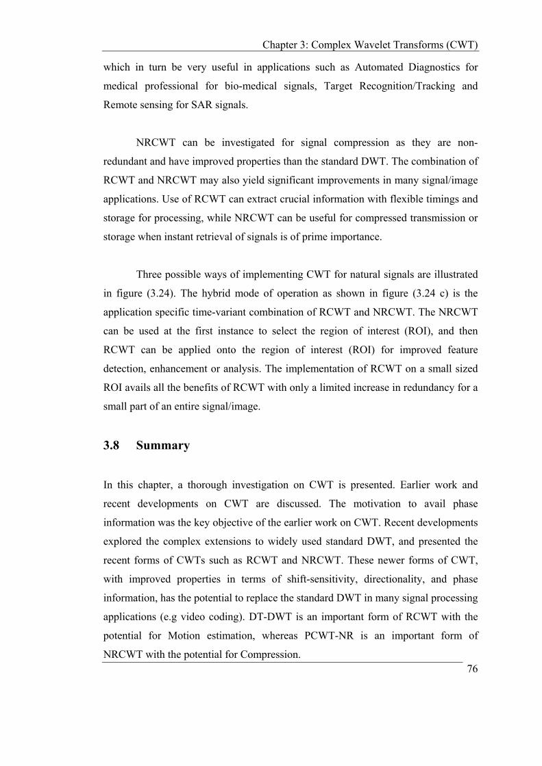
Chapter 3: Complex Wavelet Transforms (CWT)
which in turn be very useful in applications such as Automated Diagnostics for
medical professional for bio-medical signals, Target Recognition/Tracking and
Remote sensing for SAR signals.
NRCWT can be investigated for signal compression as they are non-
redundant and have improved properties than the standard DWT. The combination of
RCWT and NRCWT may also yield significant improvements in many signal/image
applications. Use of RCWT can extract crucial information with flexible timings and
storage for processing, while NRCWT can be useful for compressed transmission or
storage when instant retrieval of signals is of prime importance.
Three possible ways of implementing CWT for natural signals are illustrated
in figure (3.24). The hybrid mode of operation as shown in figure (3.24 c) is the
application specific time-variant combination of RCWT and NRCWT. The NRCWT
can be used at the first instance to select the region of interest (ROI), and then
RCWT can be applied onto the region of interest (ROI) for improved feature
detection, enhancement or analysis. The implementation of RCWT on a small sized
ROI avails all the benefits of RCWT with only a limited increase in redundancy for a
small part of an entire signal/image.
3.8 Summary
In this chapter, a thorough investigation on CWT is presented. Earlier work and
recent developments on CWT are discussed. The motivation to avail phase
information was the key objective of the earlier work on CWT. Recent developments
explored the complex extensions to widely used standard DWT, and presented the
recent forms of CWTs such as RCWT and NRCWT. These newer forms of CWT,
with improved properties in terms of shift-sensitivity, directionality, and phase
information, has the potential to replace the standard DWT in many signal processing
applications (e.g video coding). DT-DWT is an important form of RCWT with the
potential for Motion estimation, whereas PCWT-NR is an important form of
NRCWT with the potential for Compression. 76

Chapter 3: Complex Wavelet Transforms (CWT)
T
ype
Features
Standard
DWT
RCWT
DT-DWT(K)
DT-DWT(S)
NRCWT
PCWT-CR
PCWT-NR (CDDWT)
OHCWT
Proposed by Mallat
[27]
Kingsbury
[93]
Selesnick
[98]
Fernandes
[101, 114]
Fernandes
[101,114]
Spaendonck et
al [103]
Key
identification
feature
Multilevel
Resolution
Two parallel
standard
DWT
trees in
quadrature
Two parallel
standard
DWT
trees in
quadrature
Redundant
complex
mapping
followed by
any DWT or
vice versa
Non-
redundant
complex
mapping
followed by
any DWT or
vice versa
3-band structure
with two
conjugate high
pass filters
decimated by 4
Shift-
invariance
No
Poor
Yes
Very good
Yes
Very good
Yes
Good
No
Poor
No
Poor
Directionality
(for 2-D)
Poor
3 at each
level
Very good
6 at each
level for
each tree
Very good
6 at each
level for
each tree
Good
6 at each
level
Fair
6 at each
level
with
distortion in
image shape
in LH and
HL subbands
Fair
6 at each level
Phase
Information
No Yes
Very good
Yes
Very good
Yes
Good
Yes
Fair
Yes
Fair
Redundancy
(for 2-D)
No
1:1
Fixed
4:1
Fixed
4:1
Flexible
but
>= 4:1
Flexible
1:1 with
standard
DWT, and
2.67 with
DDWT
No
1:1
Table 3.2: Comparative summary of complex wavelet transforms (Contd.)
77
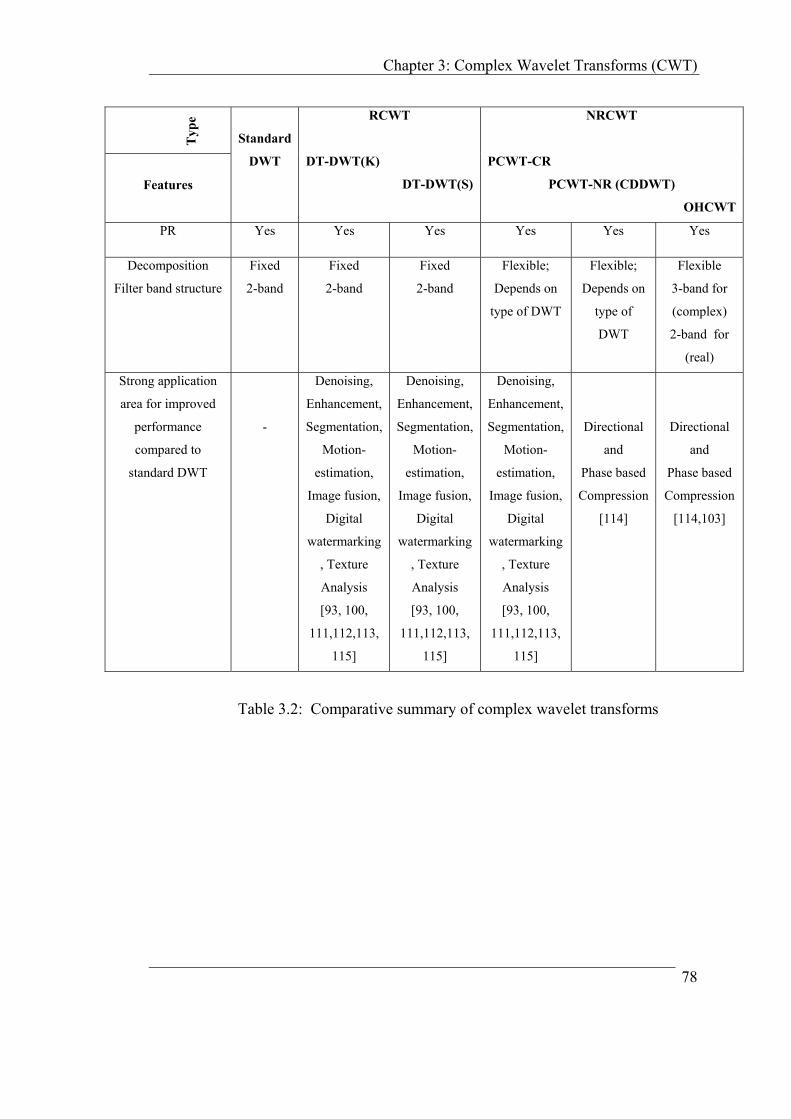
Chapter 3: Complex Wavelet Transforms (CWT)
T
ype
Features
NRCWT
PCWT-CR
PCWT-NR (CDDWT)
OHCWT
PR Yes Yes Yes Yes Yes Yes
Decomposition
Filter band structure
Fixed
2-band
Fixed
2-band
Fixed
2-band
Flexible; Flexible;
Depends on
type of
DWT
Flexible
3-band for
(complex)
2-band for
(real)
Strong application
area for improved
performance
compared to
standard DWT
-
Denoising,
Enhancement,
Segmentation,
Motion-
estimation,
Image fusion,
Digital
watermarking
, Texture
Analysis
[93, 100,
111,112,113,
115]
Denoising,
Enhancement,
Segmentation,
Motion-
estimation,
Image fusion,
Digital
watermarking
, Texture
Analysis
[93, 100,
111,112,113,
115]
Denoising,
Enhancement,
Segmentation,
Motion-
estimation,
Image fusion,
Digital
watermarking
, Texture
Analysis
[93, 100,
111,112,113,
115]
Directional
and
Phase based
Compression
[114]
Directional
and
Phase based
Compression
[114,103]
RCWT
Standard
DWT DT-DWT(K)
DT-DWT(S)
Depends on
type of DWT
Table 3.2: Comparative summary of complex wavelet transforms
78

Chapter 3: Complex Wavelet Transforms (CWT)
source forward
RCWT
inverse
RCWT
redundancy (1:2 for 1-D)
processingon
coefficients
analysis
a. Redundant processing: when redundancy is allowed for analysis, improved
processing (denoising, enhancement, estimation) or for feature detection.
source forward NRCWT
inverse
NRCWT
redundancy (≈1:1)
instant retrieval
transmission
storage
compressedcoefficients
lossy
b. Non-redundant processing: when non-redundancy is of prime importance for
high-resolution compression in transmission or storage at the cost of shift-
invariance.
non-redundant
processing
redundant processing
1 (a) 1 (a)
2 (b) 2 (b)
3 (c)
3 (c)
source sink hybrid-mode
c. Hybrid processing: 1(a) for denoising, enhancement or motion estimation 2(b)
for compression: transmission and storage, 3(c) for time-context variant
applications based on ROI
Figure 3.24: Three possible ways of implementing CWT for natural signals
79

Chapter 4: Application I- Denoising
Chapter 4:
Application I- Denoising
4.1 Introduction
Many scientific experiments result in a datasets corrupted with noise, either because
of the data acquisition process, or because of environmental effects. A first pre-
processing step in analyzing such datasets is denoising, that is, estimating the
unknown signal of interest from the available noisy data. There are several different
approaches to denoise signals and images. Despite similar visual effects, there are
subtle differences between denoising, de-blurring, smoothing and restoration.
Generally smoothing removes high frequency and retains low frequency
(with blurring), de-blurring increases the sharpness signal features by boosting the
high frequencies, whereas denoising tries to remove whatever noise is present
regardless of the spectral content of a noisy signal [116]. Restoration is kind of
denoising that tries to retrieve the original signal with optimal balancing of de-
blurring and smoothing. Traditional smoothing filters such as Mean, Median and
Gaussian filters are liner operators normally employed in spatial domain, which
smooth the signals with blurring effects [117-119].
80
A frequency domain approach (high pass) of ‘Inverse’ filtering for de-
blurring [120] is sensitive to noise, and is not alone suitable for denoising. The
Wiener filtering executes an optimal tradeoff (in MSE sense) between inverse

Chapter 4: Application I- Denoising filtering and noise smoothing. It is useful in restoration by removing the additive
noise and inverting the blurring simultaneously [120-122]. Wavelet based denoising
schemes, widely popular since last decade, are non-linear thresholding of wavelet
coefficients in time-scale transform domain.
Recent advances in wavelet based denoising combine variants of wavelet
transforms with computationally involved Hidden Markov models, spatially adaptive
methods and interscale dependency [125, 137-139] for improved performance.
Newer generations of basis functions such as Ridgelets, Curvelets and Contourlets
[140-142] have shown noticeable effectiveness over wavelets for images and higher
dimensional data processing employing complicated mathematical models.
The fundamental concepts and classifications of Wavelet Transforms (WTs)
and Complex Wavelet Transforms (CWTs) are discussed in Chapter 2 and Chapter 3
respectively. Some of the numerous applications of WTs and CWTs in many diverse
fields are enlisted in sections 2.6 and 3.7 respectively. The basic purpose of this
chapter is to describe the implementation of CWTs for Denoising. For critical
evaluation, the performance of redundant CWTs (DT-DWT(K) and DT-DWT(S)) is
compared with suitable type(s) of WTs and other conventional approaches.
Chapter 4 is organised into six sections. Section 4.1 is an introduction.
Section 4.2 describes the concept of signal and image denoising in wavelet domain.
Section 4.3 discusses generalised 1-D denoising, and section 4.4 is about a special
case of 1-D denoising for audio signals. Section 4.5 presents 2-D denoising for
various images. Section 4.6 is the conclusion for denoising application.
4.2 Wavelet Shrinkage Denoising
4.2.1 Basic Concept
Wavelet Thresholding, Wavelet Shrinkage, and Non-linear Shrinkage are widely
used terms for wavelet domain denoising. Denoising by thresholding in wavelet
81

Chapter 4: Application I- Denoising domain has been developed principally by Donoho et al. [123,124]. In wavelet
domain, large coefficients correspond to the signal, and small ones represent mostly
noise. The denoised data is obtained by inverse-transforming the suitably
thresholded, or shrunk, coefficients.
4.2.2 Shrinkage Strategies
The standard thresholding of wavelet coefficients is governed mainly by either ‘hard’
or ‘soft’ thresholding function as shown in figure (4.1). The first function in figure
(4.1 a) is a ‘liner’ function, which is not useful for denoising, as it does not alter the
coefficients. The ‘linear’ characteristic is presented in the figure just for comparing
the non-linearity of other two functions.
The hard thresholding function is given as:
z = ( ) λ>= www ,hard , and
z = ( ) λ<== wwhard ,0 (4.1)
where, w and z are the input and output wavelet coefficients respectively. λ is a
threshold value selected.
Similarly, soft thresholding function is given as:
( ) )0,max()sgn( λ−⋅== wwwsoftz , λ>w and
( ) 0== wsoftz , λ<=w (4.2)
output
input
Slope =1
a
-λ λ
-λ λ
Figure 4.1: Thresholding functions
b c
; (a) linear, (b) hard, (c) soft
82

Chapter 4: Application I- Denoising In hard thresholding, the wavelet coefficients (at each level) below threshold
λ are made zero and coefficients above threshold are not changed whereas in soft
thresholding, the wavelet coefficients are shrunk towards zero by an offset λ .
Generally soft thresholding gives fewer artifacts and preserves the smoothness. The
choice of threshold value is very crucial for a given signal for denoising.
Donoho et al. [123,124] introduced various shrinkage rules based on different
threshold values and thresholding functions such as ‘visushrink’ with fixed universal
threshold n2log2σλ = and ‘sureshrink’ based on Stein’s Unbiased Risk
Estimator (SURE), where λ is not fixed but statistically related to the associated
transform domain data sets.
There are other variants of thresholds and thresholding functions optimised
for specific applications (e.g. MRI, Ultrasonic and SAR signal processing) that
shrink the wavelet coefficients in between hard and soft thresholding under varying
noise distributions [125-132]. Typically, wavelet based denoising is performed with
fast and space saving decimated wavelet transforms. It is observed that the use of
non-decimated transforms minimizes the artifacts in the denoised data [133-135]. In
[136], it is demonstrated that the complex wavelet transforms (CWTs), being more
directional, posses a good potential to tradeoff the denoising performance with its
limited redundancy.
4.3 1-D Denoising In section 4.3, level adaptive thresholding (hard and soft) is applied separately for
each subband of 1-D signal using standard DWT, WP, SWT and redundant CWTs
(DT-DWT(K) and DT-DWT(S)) for a comparative investigation.
4.3.1 Signal and Noise Model
Signal and noise model for 1-D denoising simulations is given as:
)()()( ngnsnx σ+= , n = 1 to N (4.3)
83

Chapter 4: Application I- Denoising where, s(n) is an N point original signal, x(n) is a noisy signal corrupted by (0,1)
additive white Gaussian noise g(n) with a spread of σ as standard deviation. For
experiment, a number of signals with varying degree of smoothness (blocks, bumps,
heavy sine etc) and of various SNR are generated using Matlab function ‘wnoise’.
4.3.2 Shrinkage Strategy
Level adaptive threshold values are selected in transform domain based on various
strategies (rigrsure, heursure etc) using Matlab function ‘thselect’ and actual hard or
soft thresholding is performed using Matlab function ‘wthresh’
4.3.3 Algorithm
The wavelet shrinkage denoising of 1-D noisy signal x(n), in order to recover y(n) as
an estimate of original signal s(n) is represented as a 4-step algorithm [116] with j as
decomposition levels, W as forward WT and W-1 as inverse WT.
1. ωj = W(x), j = 1 to J
2. λj = Level adaptive threshold selection (ωj)
3. zj = Thresholding(ωj, λj)
4. y = W-1(zj)
The standard DWT is performed with Matlab (wavelet toolbox) functions
‘wavedec’ and ‘waverec’, wavelet packet (WP) algorithm is implemented with
functions ‘wpdec’, ‘bestree’, ‘wprec’ and with various tree management utilities
available. The SWT is implemented with functions ‘swt’ and ‘iswt’. The DT-DWT
algorithms employing DT-DWT(K) and DT-DWT(S) are implemented with Matlab
following the discussion given in section 3.5.
84

Chapter 4: Application I- Denoising 4.3.4 Performance Measure
The performance of various denoising algorithms is quantitatively compared using
MSE (mean square error) and SNR (signal to noise ratio) as:
MSE = 2
1)()(1 ∑
=
−N
nnyns
N
SNR = 10 log10
−∑
∑
=
=2
1
1
2
)()(
)(
N
n
N
n
nyns
ns (4.4)
where, s(n) is an original signal and y(n) is an estimate of s(n) after denoising.
The qualitative performance is compared by plotting the original and recovered
signals based on human visual perspective.
4.3.5 Results and Discussion
Some sample results of experiment to compare performance measures for various
signals under different SNR conditions are shown in tables (4.1) to (4.5). Figures (4.2
a) and (4.2 b) show the qualitative comparisons of denoising of 1-D ‘blocks’ signal
using various WTs for ‘rigrsure’ case of table (4.1). Where MSEi = initial MSE of
noisy signal, SNRi= initial SNR of noisy signal. MSEh, MSEs = MSE after hard and
soft thresholding respectively.
After observing and analysing the statistics of large number of experiments,
the conclusions are as follows:
1. The ‘rigrsure’ and ‘minimax’ are optimum for soft and hard thresholding
respectively. The threshold value selection based on ‘rigrsure’ is based on
SURE criteria and is suitable for level adaptive thresholding with various
amounts of noise and for large range of decomposition levels.
85
Chapter 4: Application I- Denoising 2. Though threshold value with ‘sqtwolog’ gives the best performance with hard
thresholding in case of ‘blocks’, it is not suitable for all types of signals with
varying degree of noise and decomposition levels.
3. Denoising performance varies with type of signal under consideration.
4. Redundant CWT namely DT-DWT(K) and DT-DWT(S) perform better than
standard DWT and WP but slightly poorer than SWT.
5. Standard DWT has improved performance than the entropy based WP. In
case of very high SNR, standard DWT and entropy based WP have the same
results because under this condition the best tree is same as standard DWT
tree.
6. Denoising with DT-DWT(K) is slightly superior than DT-DWT(S). In poor
SNR conditions, DT-DWT(K) performs equally well with either hard of soft
thresholding.
7. DT-DWT(K) gives better performance with hard thresholding whereas DT-
DWT(S) gives improved performance with soft thresholding.
8. Increasing the filter tap length improves the denoising performance with hard
thresholding but degrades the SNR and MSE with soft thresholding. There is
no change in performance of DT-DWT algorithms, as the filter lengths are
kept fixed for both DT-DWT.
9. Increase in decomposition levels (J=8) degrades the performance of standard
DWT, and SWT with soft thresholding. It also degrades the performance of
WP, DT-DWT(K) and DT-DWT(S) for both hard and soft thresholding.
86

Chapter 4: Application I- Denoising Performance
Measure
DWT WP SWT DT-
DWT(K)
DT-
DWT(S)
Threshold criteria: ‘rigrsure’
MSEh 0.63 0.76 0.54 0.24 0.52
MSEs 0.24 0.31 0.19 0.29 0.23
SNRh (dB) 17.53 16.73 18.23 21.81 18.36
SNRs (dB) 21.69 20.64 22.68 20.86 21.90
Threshold criteria: ‘heursure’
MSEh 0.37 0.47 0.24 0.32 0.27
MSEs 0.37 0.40 0.31 0.57 0.31
SNRh (dB) 19.84 18.85 21.84 20.53 21.21
SNRs (dB) 19.86 19.52 20.65 17.98 20.59
Threshold criteria: ‘sqtwolog’
MSEh 0.27 0.37 0.14 0.34 0.19
MSEs 0.55 0.58 0.52 0.37 0.49
SNRh (dB) 21.17 19.87 24.07 20.30 22.82
SNRs (dB) 18.17 17.93 18.40 16.93 18.63
Threshold criteria: ‘minimaxi’
MSEh 0.43 0.61 0.22 0.20 0.37
MSEs 0.27 0.32 0.26 0.37 0.25
SNRh (dB) 19.18 17.70 22.16 22.64 19.85
SNRs (dB) 21.21 20.44 21.43 19.86 21.50
Table 4.1: Effect of thresholding criteria for 1-D denoising on a signal ‘blocks’ with N=1024 points, initial SNRi= 15.36 dB, MSEi= 1.05, level of WT decomposition J=4, wavelet type for DWT, WP and SWT is ‘db2’, filters for DT-DWT(K) are ‘near_sym_b’ and ‘qshift_b’ as given in appendix A, filters for DT-DWT(S) are as given in appendix B.
87

Chapter 4: Application I- Denoising
Performance
Measure
DWT WP SWT DT-
DWT(K)
DT-
DWT(S)
Signal: ‘bumps’ with SNRi= 7.18, MSEi=1.05
MSEh 0.34 0.59 0.20 0.10 0.20
MSEs 0.16 0.21 0.11 0.12 0.11
SNRh (dB) 12.11 9.70 14.37 17.18 14.36
SNRs (dB) 15.26 14.18 17.15 16.45 17.13
Signal: ‘heavy sine’ with SNRi= 20.13, MSEi= 1.05
MSEh 0.28 0.56 0.14 0.12 0.21
MSEs 0.13 0.19 0.09 0.11 0.10
SNRh (dB) 25.81 22.87 28.94 29.65 26.99
SNRs (dB) 29.17 27.64 30.94 29.80 30.50
Signal: ‘doppler’ with SNRi= 5.94, MSEi= 1.05
MSEh 0.28 0.50 0.20 0.12 0.15
MSEs 0.15 0.19 0.l0 0.11 0.11
SNRh (dB) 11.72 9.17 13.10 15.31 12.14
SNRs (dB) 14.51 13.43 16.02 15.74 15.84
Signal: ‘quad chirp’ with SNRi= 11.86, MSEi= 1.06
MSEh 1.05 0.98 1.02 0.82 1.00
MSEs 0.87 0.70 0.78 0.74 0.72
SNRh (dB) 11.84 12.11 11.97 12.91 12.03
SNRs (dB) 12.68 13.59 13.12 13.34 13.43
Table 4.2: Effect of different SNRi and MSEi for 1-D denoising with ‘rigrsure’ thresholding on various signals with N=1024 points, level of WT decomposition J= 4, wavelet type for DWT, WP and SWT is ‘db2’, filters for DT-DWT(K) (‘near_sym_b’ and ‘qshift_b’) and filters for DT-DWT(S) are as given in appendix A and B respectively.
88

Chapter 4: Application I- Denoising
Performance
Measure
DWT WP SWT DT-
DWT(K)
DT-
DWT(S)
MSEh 0.21 0.48 0.14 0.11 0.22
MSEs 0.14 0.18 0.10 0.11 0.11
SNRh (dB) 10.25 6.73 12.06 12.96 10.00
SNRs (dB) 12.11 10.91 13.44 12.97 12.97
Table 4.3: Effect of low SNRi for 1-D denoising on ‘blocks’ signal with N=1024 points, threshold criteria is ‘rigrsure’, SNRi= 3.32, MSEi=1.05, level of WT decomposition J= 4, wavelet type for DWT, WP and SWT is ‘db2’.
Performance
Measure
DWT WP SWT DT-
DWT(K)
DT-
DWT(S)
MSEh 0.61 0.72 0.53 0.24 0.52
MSEs 0.28 0.36 0.25 0.29 0.23
SNRh (dB) 17.69 17.01 18.30 21.81 18.36
SNRs (dB) 21.09 19.94 21.59 20.86 21.90
Table 4.4: Effect of long tap filters for 1-D denoising on ‘blocks’ signals with N =1024 points, threshold criteria = ‘rigrsure’, SNRi= 15.36, MSEi=1.05, level of WT decomposition J=4, wavelet type for DWT, WP and SWT = ‘db6’.
Performance
Measure
DWT WP SWT DT-
DWT(K)
DT-
DWT(S)
MSEh 0.64 0.95 0.54 0.58 0.59
MSEs 0.27 0.75 0.19 0.32 0.44
SNRh (dB) 17.53 15.76 18.24 20.51 17.36
SNRs (dB) 21.30 16.78 22.67 17.92 19.13
Table 4.5: Effect of more number of decomposition levels for 1-D denoising on ‘blocks’ signal with N=1024 points, threshold criteria = ‘rigrsure’, SNRi= 15.36, MSEi=1.05, level of WT decomposition J= 8, wavelet type for DWT, WP and SWT = ‘db2’.
89
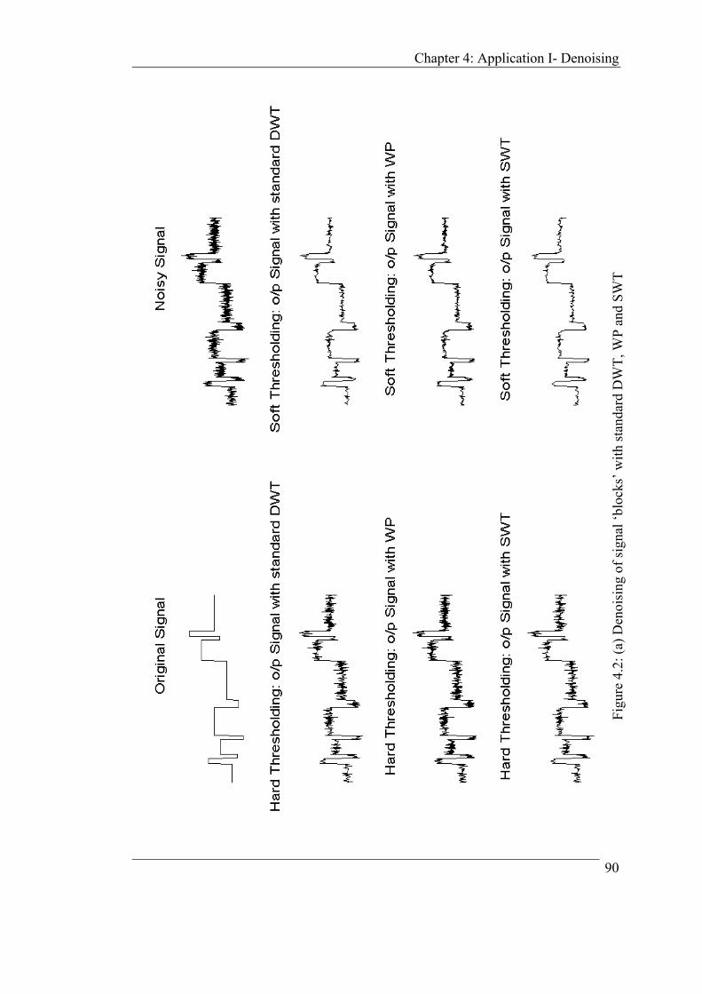
Chapter 4: Application I- Denoising
Figu
re 4
.2: (
a) D
enoi
sing
of s
igna
l ‘bl
ocks
’ with
stan
dard
DW
T, W
P an
d SW
T
90

Chapter 4: Application I- Denoising
Figu
re 4
.2: (
b) D
enoi
sing
of s
igna
l ‘bl
ocks
’ with
redu
ndan
t CW
T, D
T-D
WT(
S) a
nd D
T-D
WT(
K)
91

Chapter 4: Application I- Denoising 4.4 Audio Signal Denoising
4.4.1 WT for Audio Signals
Audio signal denoising is a special 1-D application. Traditionally audio signal
processing is based on time-frequency (STFT) representation rather than time-scale.
The choice of wavelets for audio signal processing is due to it multiresolution
properties with constant-Q filterbank, which is a suitable model for the internal
auditory processing of inner ear. The CWTs are more closely related to Fourier
techniques (due to their complex valued representation) than the real valued WTs.
The basic approach of denoising audio signal with redundant CWT (namely DT-
DWT(K)) mentioned in this section is taken from [143]. Various other approaches to
wavelet based audio signal processing can be found in [144-146].
4.4.2 Denoising Model
The traditional Fourier based model for noise reduction in many audio signals
of interest (e.g. speech, music) is known as STSA (Short Time Spectrum
Attenuation) [147]. The variant of STSA derived in wavelet domain is STWA (Short
Time Wavelet Attenuation) as shown in figure (4.3).
|Xw|
|Gw|
|Zw|
∠Xwx = s + σ g
y
g
s Short-time Analysis
(Forward WT)Suppression
rule
Noise
estimation
Short-time Analysis
(InverseWT)
Short-time Analysis
(Forward WT)
Figure 4.3: Block diagram of STWA (short time wavelet attenuation) method
92

Chapter 4: Application I- Denoising STWA is equivalent to applying a real valued gain between 0 and 1 with
threshold based offset to the wavelet coefficients at each level of the noisy
(observed) short time audio signal x(n) based on a predefined thresholding strategy in
order to get an estimated wavelet coefficients Zw for the recovered signal y(n). The
formula governing this wavelet attenuation is termed as ‘noise suppression rule’; it
depends in general on the power of signal PXw and power of noise PGw in wavelet
domain. The observed signal magnitude is termed as |Xw| and the estimate of noise
magnitude is as |Gw|. The noise estimate is assumed to be accurate as it can be
derived in the absence of actual audio signal (assuming noise remains stationary
between such observation intervals).
4.4.3 Shrinkage Strategies
The noise suppression rule in wavelet domain is based on heuristic thresholding in
order to optimise quantitative measures like MSE and SNR (defined in equation 4.4)
or qualitative human perceptual (through eyes and ears). The global thresholding is
optimised to minimise the artifacts or residual noise, which is known as bird noise,
warble, clicks, whistles or musical noise.
The approach of denoising audio signal mentioned in this section compares
the performance of standard DWT and redundant CWT. Processing of wavelet
coefficient processing is investigated with 4 different thresholding rules namely hard,
soft, Wiener filtering and raised-cosine-law. In all cases, wavelet coefficients above
predetermined threshold are unchanged but the coefficients below threshold are
attenuated in different ways with [147]
XwP = 2||∑ Xw and = GwP 2||∑ Gw as:
Hard thresholding: Threshold value (λ) = 2 GwP
Zw = Xw for Xw ||∀ ≥ λ
Zw = 0 for |Xw|∀ <λ
93
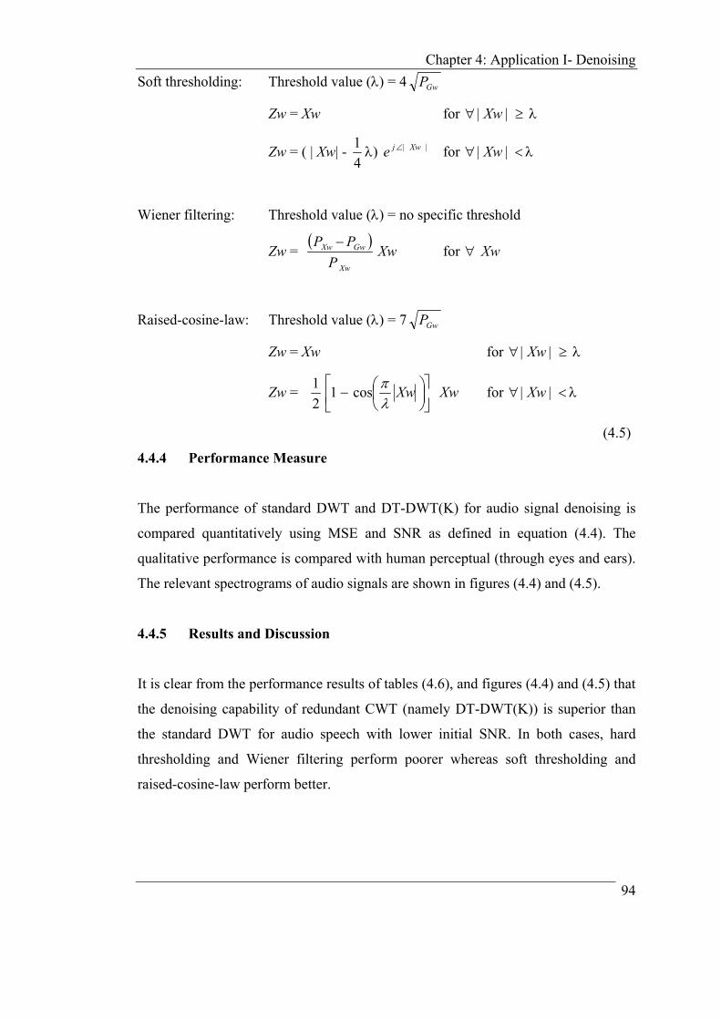
Chapter 4: Application I- Denoising Soft thresholding: Threshold value (λ) = 4 GwP
Zw = Xw for |Xw|∀ ≥ λ
Zw = ( | Xw| - 41λ) for || Xwje ∠ || Xw∀ <λ
Wiener filtering: Threshold value (λ) = no specific threshold
Zw = ( )
Xw
GwXw
PPP −
Xw for Xw∀
Raised-cosine-law: Threshold value (λ) = 7 GwP
Zw = Xw for || Xw∀ ≥ λ
Zw =
− Xwλπcos1
21 Xw for | Xw |∀ <λ
(4.5)
4.4.4 Performance Measure
The performance of standard DWT and DT-DWT(K) for audio signal denoising is
compared quantitatively using MSE and SNR as defined in equation (4.4). The
qualitative performance is compared with human perceptual (through eyes and ears).
The relevant spectrograms of audio signals are shown in figures (4.4) and (4.5).
4.4.5 Results and Discussion
It is clear from the performance results of tables (4.6), and figures (4.4) and (4.5) that
the denoising capability of redundant CWT (namely DT-DWT(K)) is superior than
the standard DWT for audio speech with lower initial SNR. In both cases, hard
thresholding and Wiener filtering perform poorer whereas soft thresholding and
raised-cosine-law perform better.
94

Chapter 4: Application I- Denoising
Methods and Initial
Parameters Standard DWT DT-DWT(K)
Thresholding Rule
MSE
MSEi= 824
SNR (dB)
SNRi= 5.00
MSE
MSEi= 824
SNR (dB)
SNRi= 5.00
Hard 343 8.81 212 10.90
Soft 237 10.40 175 11.72
Wiener 625 6.20 630 6.17
Raised-cosine 205 11.04 161 12.10
Table 4.6: The MSE and SNR of denoised audio signal (y) from the observed noisy signal (x) with respect to original signal (s). The initial value of MSE and SNR for noisy signal are MSEi= 824 , SNRi= 5.00 dB . The wavelets used for standard DWT is ‘bior6.8’ and for DT-DWT(K) is ‘near_sym_b’ and ‘qshift_b’. The maximum decomposition level employed is J = log2(N), where N = 65536 = size of audio signal. The audio signal contains a microphone quality snap shot of a male lecturer’s speech.
95
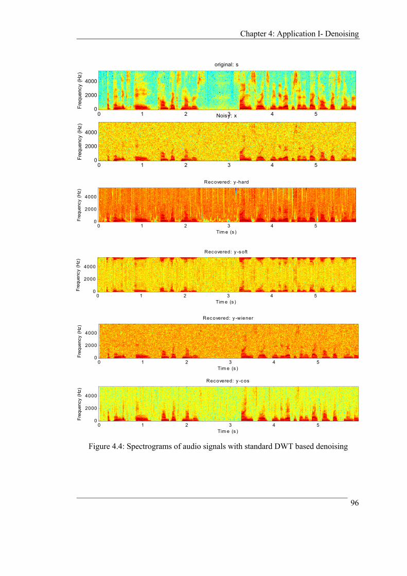
Chapter 4: Application I- Denoising
original: s
Freq
uenc
y (H
z)
0 1 2 3 4 50
2000
4000
Noisy: x
Freq
uenc
y (H
z)
0 1 2 3 4 50
2000
4000
Rec overed: y -hard
Freq
uenc
y (H
z)
Tim e (s )0 1 2 3 4 5
0
2000
4000
Rec overed: y -s oft
Freq
uenc
y (H
z)
0 1 2 3 4 50
2000
4000
Tim e (s )
Rec overed: y -wiener
Freq
uenc
y (H
z)
0
2000
4000
Ti m e (s )
0 1 2 3 4 5
Recovered: y -cos
Freq
uenc
y (H
z)
0
2000
4000
Ti m e (s )
0 1 2 3 4 5
Figure 4.4: Spectrograms of audio signals with standard DWT based denoising
96

Chapter 4: Application I- Denoising
original: s
Freq
uenc
y (H
z)
0 1 2 3 4 50
2000
4000
Noisy: x
Freq
uenc
y (H
z)
0 1 2 3 4 50
2000
4000
Rec overed: y -hard
Freq
uenc
y (H
z)
0
2000
4000
Ti m e (s )
0 1 2 3 4 5
Rec overed: y -s oft
Freq
uenc
y (H
z)
0
2000
4000
T e (s )im
0 1 2 3 4 5
Recovered: y -wiener
Freq
uenc
y (H
z)
0
2000
4000
Tim e (s )
0 1 2 3 4 5
Recovered: y -cos
Freq
uenc
y (H
z)
0 1 2 3 4 50
2000
4000
Ti e (s )m
Figure 4.5: Spectrograms of audio signals with DT-DWT(K) based denoising
97
Chapter 4: Application I- Denoising 4.5 2-D Denoising In this section 2-D denoising performance of redundant CWTs (both DT-DWT(K)
and DT-DWT(S)) is compared with other wavelet based algorithms such as standard
DWT, SWT. The results are also compared with conventional image filtering
(denoising/smoothing) methods such as Average (Mean), Median, and Wiener
filtering [148-150]. For conventional filtering methods, relevant Matlab (Image
processing toolbox) functions are employed [151].
4.5.1 Image and Noise Model
The standard test images such as Lenna, Goldhill, Peppers, Airplane and Pattern are
taken for experiments (see Appendix C). Original images are corrupted by additive
white Gaussian noise.
The image and noise model is given as:
x = s + σ⋅g
where, s is an original image and x is a noisy image corrupted by additive white
Gaussian noise g of standard deviation σ. Both images s and x are of size N by M
(mostly M =N and always power of 2).
4.5.2 Shrinkage Strategy
All wavelet-based algorithms in this section determine the optimum threshold value
iteratively with a selected resolution-step size from ‘stpsz’ = {1,2,5,10} to minimize
the MSE for both hard and soft thresholding options separately.
4.5.3 Algorithm
2-D denoising is an extension of 1-D denoising based on 2-D separable WT
implementation (discussed in section 2.5.1). The basic algorithm for wavelet
shrinkage denoising remains same as listed in section 4.3.3 but is applied to the
matrix of 2-D data.
98

Chapter 4: Application I- Denoising For all conventional filtering methods, 3-by-3 filter kernel is taken for
convolution. For all wavelet based methods, decomposition is performed up to J
levels. For standard DWT and SWT the arbitrary wavelet basis employed is ‘wtype’.
Filters for DT-DWT(K) (‘wtype-k’), and DT-DWT(S) (‘wtype-s’), are given in
Appendix A and B respectively.
4.5.4 Performance Measure
The quantitative measures for 2-D denoising, namely MSE (Mean Square error) and
PSNR (Peak Signal to Noise Ratio) are determined as:
MSE = [ ]2
1 1),(),(1 ∑ ∑
= =
−N
n
M
mmnymns
NM
PSNR = 10 log10
MSE255
(4.7)
where, s is an original image and y is a recovered image from a noisy image x.
The qualitative performance is evaluated through human visual system by
observing the recovered images with various algorithms.
4.5.5 Results and Discussion
A few sample results of denoising performance (using various methods) based on
quantitative measure are presented in tables (4.7) to (4.12) and the qualitative
performance based on human visual system for various algorithms are shown in
figures (4.6) to (4.15).
The performance results of various algorithms can be evaluated for low and high
noise conditions as follows:
99

Chapter 4: Application I- Denoising 1. Under low noise conditions (σ=10), conventional filtering methods namely
Median and Weiner perform better than standard DWT. Though the
performance of Mean filter is poorer than standard DWT.
2. The denoising capability (σ=10) of both DT-DWTs is better than SWT and
standard DWT for all natural images as well as for synthetic ‘Pattern’ image.
The performance of both DT-DWTs is nearly same with DT-DWT(K)
slightly better then DT-DWT(S).
3. Under high noise conditions (σ=40), all conventional filtering methods give
poor denoising results than even standard DWT. For all images, performance
of both DT-DWTs is better than SWT and standard DWT. The performance
of DT-DWT(K) is the best using both hard and soft thresholding.
4. The lowest values of optimum threshold (for both hard and soft thresholding)
for DT-DWT(K) in all noise conditions (σ= 10 or 40) suggest its superior
denoising capabilities with improved feature preservation (with less blurring).
5. The effect of improved directionality on denoising for redundant CWT (both
DT-DWTs) compared to less directional standard DWT is quite clear for
‘pattern’ image for all noise conditions.
6. From human visual perspective, the performance of various algorithms for
high noise conditions is quite clear. The performance of DT-DWTs is
distinguishably superior to standard DWT. But under low noise conditions,
minute differences are very difficult to perceive hence all wavelet based
methods seem to have nearly same visual effects.
100

Chapter 4: Application I- Denoising
Images with σ =10 Performance Measure
for
Denoising Methods Lenna Goldhill Peppers Airplane Pattern
Initial MSE (MSEi) 100 100 100 100 99
(a) MSE (Conventional filtering)
Mean 68 75 57 64 153
Median 60 65 41 44 69
Wiener 40 42 30 28 67
(b) MSE (Hard thresholding)
Standard DWT 56 65 43 45 79
SWT 39 41 28 26 42
DT-DWT(K) 35 39 27 24 29
DT-DWT(S) 35 38 26 23 30
(c) MSE (Soft thresholding)
Standard DWT 44 48 38 40 63
SWT 36 39 28 28 47
DT-DWT(K) 33 37 27 27 35
DT-DWT(S) 33 37 27 27 38
Table 4.7: MSE for various denoising methods (σ =10) for different images: (a) Conventional filtering (b) Hard thresholding (c) Soft thresholding with parameters J=3, stpsz =1, wtype = ‘db2’, wtype-k = ‘near_sym_b’ and ‘qshift_b’, wtype-s = ‘FSfilt’ and ‘otherfilt’.
101

Chapter 4: Application I- Denoising
Images with σ =10 Performance Measure
for
Denoising Methods
Lenna Goldhill Peppers Airplane Pattern
Initial PSNR (PSNRi in dB)
28.12 28.15 28.12 28.12 28.15
(a) PSNR in dB (Conventional filtering)
Mean 29.82 29.34 30.57 30.02 26.26
Median 30.35 29.99 32.02 31.71 29.69
Wiener 32.08 31.87 33.33 33.62 29.82
(b) PSNR in dB (Hard thresholding)
Standard DWT 30.63 29.99 31.71 31.52 29.15
SWT 32.24 31.95 33.65 33.93 31.88
DT-DWT(K) 32.65 32.19 33.75 34.25 33.49
DT-DWT(S) 32.64 32.25 33.84 34.38 33.28
(c) PSNR in dB (Soft thresholding)
Standard DWT 31.65 31.28 32.23 32.10 30.14
SWT 32.59 32.18 33.60 33.53 31.39
DT-DWT(K) 32.91 32.37 33.77 33.77 32.65
DT-DWT(S) 32.87 32.33 33.77 33.76 32.27
Table 4.8: PSNR for various denoising methods (σ =10) for different images: (a) Conventional filtering (b) Hard thresholding (c) Soft thresholding with parameters J=3, stpsz =1, wtype = ‘db2’, wtype-k = ‘near_sym_b’ and ‘qshift_b’, wtype-s = ‘FSfilt’ and ‘otherfilt’.
102

Chapter 4: Application I- Denoising
Images with σ =10 Denoising Methods
Lenna Goldhill Peppers Airplane Pattern
(a) Optimum threshold value (λh)
for Hard thresholding
Standard DWT 30 27 30 28 22
SWT 28 27 31 30 30
DT-DWT(K) 16 15 17 17 17
DT-DWT(S) 32 30 35 34 35
(b) Optimum threshold value (λs)
for Soft thresholding
Standard DWT 11 10 12 11 7
SWT 12 11 14 13 11
DT-DWT(K) 7 7 8 8 7
DT-DWT(S) 15 14 16 16 14
Table 4.9: Optimum threshold value for various denoising methods (σ =10) for different images: (a) Hard Thresholding λh (b) Soft thresholding λs. with parameters J=3, stpsz =1, wtype = ‘db2’, wtype-k = ‘near_sym_b’ and ‘qshift_b’, wtype-s = ‘FSfilt’ and ‘otherfilt’. 103

Chapter 4: Application I- Denoising
Images with σ =40 Performance Measure
for
Denoising Methods Lenna Goldhill Peppers Airplane Pattern
Initial MSE (MSEi) 1593 1600 1605 1593 1595
(a) MSE (Conventional filtering)
Mean 234 242 223 231 317
Median 322 325 304 310 388
Wiener 317 322 305 301 342
(b) MSE (Hard thresholding)
Standard DWT 177 224 199 242 609
SWT 124 162 114 141 294
DT-DWT(K) 113 155 108 135 212
DT-DWT(S) 116 161 110 139 225
(c) MSE (Soft thresholding)
Standard DWT 186 224 207 240 521
SWT 133 172 137 168 376
DT-DWT(K) 121 159 125 156 252
DT-DWT(S) 124 168 129 159 275
Table 4.10: MSE for various denoising methods (σ =40) for different images: (a) Conventional filtering (b) Hard thresholding (c) Soft thresholding with parameters J=4, stpsz =1 wtype = ‘db2’, wtype-k = ‘near_sym_b’ and ‘qshift_b’, wtype-s = ‘FSfilt’ and ‘otherfilt’
104

Chapter 4: Application I- Denoising
Images with σ =40 Performance Measure
for
Denoising Methods Lenna Goldhill Peppers Airplane Pattern
Initial PSNR (PSNRi in dB)
16.11 16.09 16.10 16.10 16.10
(a) PSNR in dB (Conventional filtering)
Mean 24.45 24.28 24.60 24.50 23.10
Median 23.05 23.00 23.30 23.20 22.20
Wiener 23.12 23.06 23.30 23.40 22.80
(b) PSNR in dB (Hard thresholding)
Standard DWT 25.66 24.63 25.10 24.30 20.30
SWT 27.12 26.03 27.60 26.60 23.40
DT-DWT(K) 27.62 26.23 27.80 26.80 24.90
DT-DWT(S) 27.48 26.06 27.70 26.70 24.60
(c) PSNR in dB (Soft thresholding)
Standard DWT 25.44 24.63 25.00 24.30 21.00
SWT 26.88 25.75 26.80 25.90 22.40
DT-DWT(K) 27.30 26.09 27.10 26.20 24.10
DT-DWT(S) 27.29 25.88 27.00 26.10 23.70
Table 4.11: PSNR for various denoising methods (σ =40) for different images: (a) Conventional filtering (b) Hard thresholding (c) Soft thresholding with parameters J=4, stpsz =1, wtype = ‘db2’, wtype-k = ‘near_sym_b’ and ‘qshift_b’, wtype-s = ‘FSfilt’ and ‘otherfilt’.
105

Chapter 4: Application I- Denoising
Images with σ =40 Denoising
Methods Lenna Goldhill Peppers Airplane Pattern
(a) Optimum threshold value (λh)
for Hard thresholding
Standard DWT 146 147 140 137 117
SWT 133 131 131 128 122
DT-DWT(K) 78 75 78 75 71
DT-DWT(S) 153 147 148 142 141
(b) Optimum threshold value (λs)
for Soft thresholding
Standard DWT 75 73 71 68 50
SWT 76 71 73 69 55
DT-DWT(K) 45 43 43 41 36
DT-DWT(S) 88 83 85 80 70
Table 4.12: Optimum threshold value for various denoising methods (σ =40) for diffferent images: (a) Hard Thresholding λh (b) Soft thresholding λs with parameters J=4, stpsz =1, wtype = ‘db2’, wtype-k = ‘near_sym_b’ and ‘qshift_b’, wtype-s = ‘FSfilt’ and ‘otherfilt’.
106
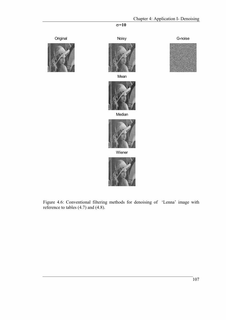
Chapter 4: Application I- Denoising σ=10
Original Noisy G-noise
Mean
Median
Wiener
Figure 4.6: Conventional filtering methods for denoising of ‘Lenna’ image with reference to tables (4.7) and (4.8).
107

Chapter 4: Application I- Denoising σ = 10, J=3
DWT-hard
100 200 300 400 500
100
200
300
400
500
DWT-soft
100 200 300 400 500
100
200
300
400
500
SWT-hard
100 200 300 400 500
100
200
300
400
500
SWT-soft
100 200 300 400 500
100
200
300
400
500
DT-DWT(K)-hard
100 200 300 400 500
100
200
300
400
500
DT-DWT(K)-soft
100 200 300 400 500
100
200
300
400
500
DT-DWT(S)-hard
100 200 300 400 500
100
200
300
400
500
DT-DWT(S)-soft
100 200 300 400 500
100
200
300
400
500
Figure 4.7: Wavelet Transform based methods for denoising of ‘Lenna’ image with reference to tables (4.7) to (4.9).
108
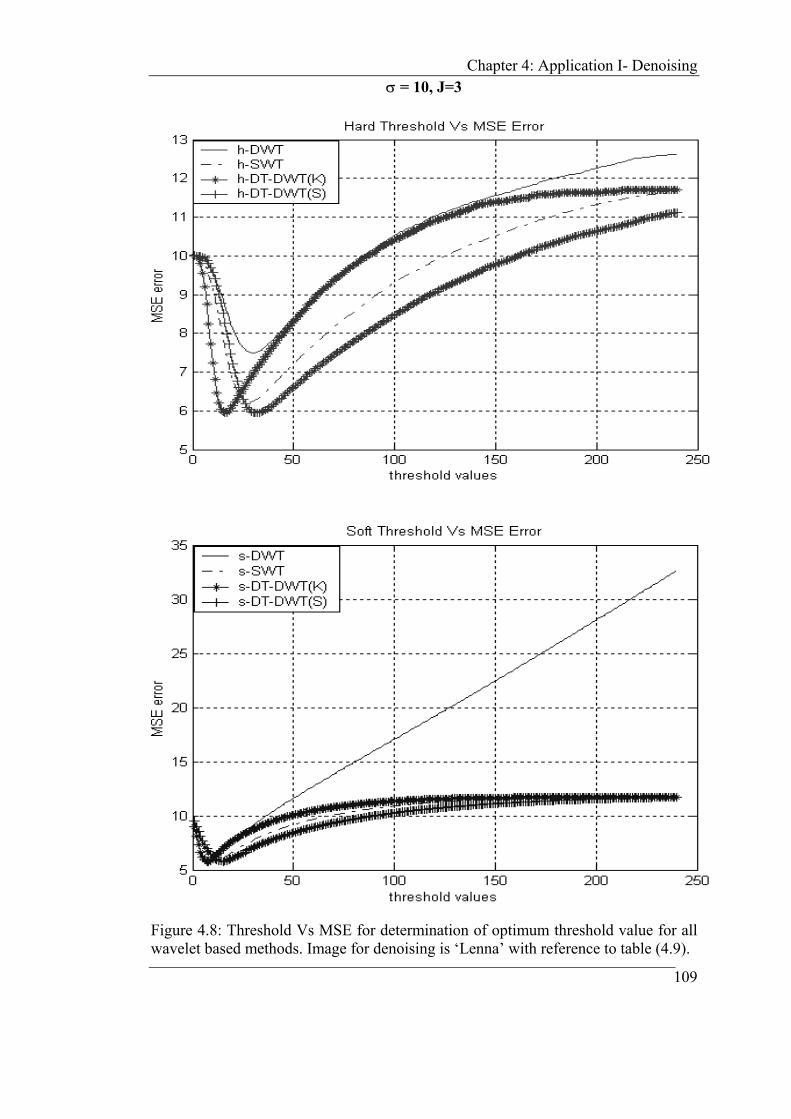
Chapter 4: Application I- Denoising σ = 10, J=3
Figure 4.8: Threshold Vs MSE for determination of optimum threshold value for all wavelet based methods. Image for denoising is ‘Lenna’ with reference to table (4.9).
109

Chapter 4: Application I- Denoising σ = 40
Original Noisy G-noise
Mean
Median
Wiener
Figure 4.9: Conventional filtering methods for denoising of ‘Lenna’ image with reference to tables (4.10) and (4.11).
110
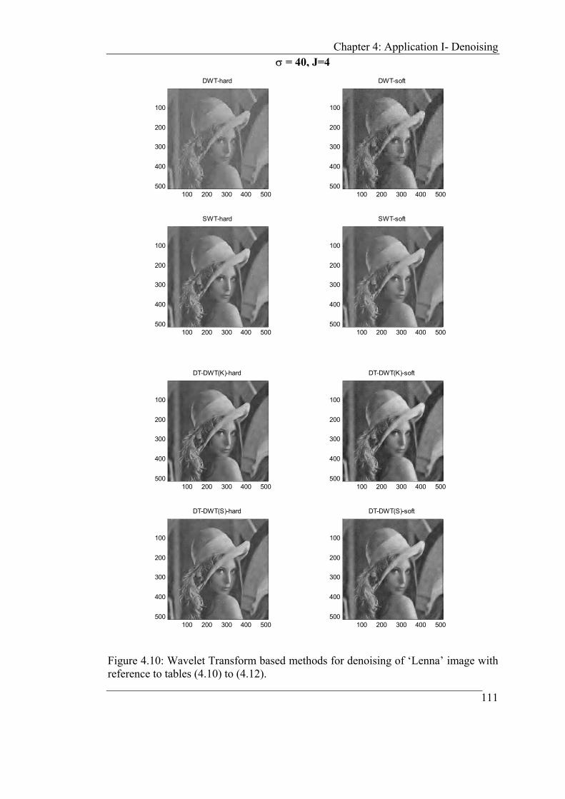
Chapter 4: Application I- Denoising σ = 40, J=4
DWT-hard
100 200 300 400 500
100
200
300
400
500
DWT-soft
100 200 300 400 500
100
200
300
400
500
SWT-hard
100 200 300 400 500
100
200
300
400
500
SWT-soft
100 200 300 400 500
100
200
300
400
500
DT-DWT(K)-hard
100 200 300 400 500
100
200
300
400
500
DT-DWT(K)-soft
100 200 300 400 500
100
200
300
400
500
DT-DWT(S)-hard
100 200 300 400 500
100
200
300
400
500
DT-DWT(S)-soft
100 200 300 400 500
100
200
300
400
500
Figure 4.10: Wavelet Transform based methods for denoising of ‘Lenna’ image with reference to tables (4.10) to (4.12).
111

Chapter 4: Application I- Denoising σ = 40, J=4
Figure 4.11: Threshold Vs MSE for determination of optimum threshold value for all wavelet based methods. Image for denoising is ‘Lenna’ with reference to table (4.12). 112

Chapter 4: Application I- Denoising
DWT:hard
50 100 150 200 250 300 350 400 450 500
50
100
150
200
250
300
350
400
450
500
DWT:soft
50 100 150 200 250 300 350 400 450 500
50
100
150
200
250
300
350
400
450
500
Figure 4.12: DWT based denoising of ‘Lenna’ image using hard and soft thresholding with reference to tables (4.10) to (4.12).
113

Chapter 4: Application I- Denoising
SWT:hard
50 100 150 200 250 300 350 400 450 500
50
100
150
200
250
300
350
400
450
500
SWT:soft
50 100 150 200 250 300 350 400 450 500
50
100
150
200
250
300
350
400
450
500
Figure 4.13: SWT based denoising of ‘Lenna’ image using hard and soft thresholding with reference to tables (4.10) to (4.12).
114

Chapter 4: Application I- Denoising
DT-DWT(K)-hard
50 100 150 200 250 300 350 400 450 500
50
100
150
200
250
300
350
400
450
500
DT-DWT(K)-soft
50 100 150 200 250 300 350 400 450 500
50
100
150
200
250
300
350
400
450
500
Figure 4.14: DT-DWT(K) based denoising of ‘Lenna’ image using hard and soft thresholding with reference to tables (4.10) to (4.12).
115

Chapter 4: Application I- Denoising
DT-DWT(S)-hard
50 100 150 200 250 300 350 400 450 500
50
100
150
200
250
300
350
400
450
500
DT-DWT(S)-soft
50 100 150 200 250 300 350 400 450 500
50
100
150
200
250
300
350
400
450
500
Figure 4.15: DT-DWT(S) based denoising of ‘Lenna’ image using hard and soft thresholding with reference to tables (4.10) to (4.12).
116
Chapter 4: Application I- Denoising 4.6 Conclusion
It is concluded that DT-DWTs are superior to standard DWT for all 1-D and 2-D
denoising application. The choice of shrinkage (thresholding) strategy, and selection
of optimum threshold value are very crucial for wavelet shrinkage denoising using
any form of WT. DT-DWTs are especially efficient in higher noise conditions.
Entropy based WP is not suitable for generalised denoising applications in poor SNR
conditions. Almost equal performance of limited redundant DT-DWT with other
advantages makes it a promising choice over highly redundant SWT for signal and
image denoising applications.
117

Chapter 5: Application II- Edge Detection
Chapter 5:
Application II- Edge Detection
5.1 Introduction
For many natural signals the vital information about its originating source, external
environment, processing, and the characterisation of important features is closely
linked with the transients (or local singularities, edges) in those signals under
consideration [148,150,152-154]. For 1-D signal, edge is considered as a distinct
observable variation in the smoothness or continuity. For 2-D, image intensity is
often proportional to scene radiance, physical edges (corresponding to the significant
variations in reflectance, illumination, orientation and depth of scene surfaces) are
represented in the image by changes in the intensity function.
Due to wealth of information associated with edges, edge detection is an
important task for many applications related to computer vision and pattern
recognition [154,155]. There are various categories of edges such as step, ramp,
exponential or certain non-deterministic singularities with varying degree of
sharpness [156]. Steps (and its combinations) are the most common type of edge
encountered. This type of edges result from various phenomena; for example when
one object hides another, or when there is shadow on a surface. It generally occurs
between two regions having almost common, but different grey levels.
118

Chapter 5: Application II- Edge Detection Chapter 5 is organised into five sections. Section 5.1 is an introduction.
Section 5.2 presents the survey of various classical edge detection approaches and
highlights a few important multiscale approaches. Section 5.3 is about 1-D edge
detection in higher noise environment using multiscale algorithms. In this section,
existing algorithms are critically reviewed and compared with individually developed
new algorithms. In section 5.4, a very simple 2-D edge detection methodology is
presented to compare edge detection performance of the extensions of DWT with
DT-DWT(K). Section 5.5 is the conclusion of the study of edge detection.
5.2 Edge Detection Approaches
5.2.1 Classical Approaches
In a function, singularities can be characterised as discontinuities where derivative(s)
or gradient approaches infinity. However, if the signal data is discrete, then the edges
are often defined as the local maxima of the derivative(s). Essentially an edge
detector is a high pass filter (operator) that can be applied to extract the edge points
in a signal [118,148,150]. The classical 2-D gradient operators such as Roberts,
Prewitt, Sobel and Fri-Chen for edge detection reduce to an FIR filter with impulse
response [-1,0,1] in 1-D [148]. All these operators being high pass filters are
sensitive to noise (especially widely used AWGN) [157].
To combat with noise, more general robust extensions, so-called filtered
derivate methods (e.g. Marr and Hildreth) are devised [158-160]. These pre-
smoothing approaches combine various smoothing operators (e.g Gaussian) with
gradient estimation are more effective in higher noise conditions and are attractive
due to low complexity linear implementation. The weakness of all above approaches
is that the optimal result may not be obtained by using a fixed size operator.
Attempting to achieve simultaneously detection and localisation of an edge results in
a tradeoff between the level of smoothing and the accuracy of estimated edge
location. The tradeoff is also sensitive to category of edge (sharp or smooth) and
SNR of the signal. Canny [161] in his computational approach to edge detection
119

Chapter 5: Application II- Edge Detection showed exploited such tradeoff and derived an improved edge detector for noisy
environment by different size kernels in filtered derivative method with non-
maximum suppression and dual thresholding.
Various attempts for edge detection in noisy conditions are based on
combinations of many different explicit and heuristic models (e.g. liner filtering,
covariance models, dispersion of gradient, regularisation, statistics, neural networks,
genetic algorithms, fuzzy reasoning etc.) in order to closely approximate the
uncertainty of noise distributions. Most of these attempts compare the results with
well-known detectors such as Sobel, Canny, DoG, and LoG. Because of only
qualitative performance comparisons (without well accepted objective performance
measure based on ground-truth calibration), there is a belief that edge detection
algorithms are reaching an asymptotic level of performance [162].
5.2.2 Multiscale Approaches
The developments in the field of multi-resolution wavelet transforms with their
ability to detect and characterise singularities, attracted many researchers to explore
the optimal edge detection problem in higher noise conditions [163-166,176,177].
The advantage with multiscale approach is its inherent implementation, with variable
size derivative operators at various scales, to tradeoff between detection and
localisation of local singularities. The indirect inter-dependence of wavelet
coefficients at different scales opens the possibility to explore the hidden association
of information at various scales (levels).
The important investigations of multiscale edge detection include MZ-MED
(Mallat and Zong’s Multiscale Edge Detection) based on modulus maxima evolution
from course to fine scales [164], multiscale products by Xu et.al. [165] based on
Rosenfeld’s idea of cross-scale correlation [166]. A few other multiscale singularity
detection approaches are as [167-170].
120

Chapter 5: Application II- Edge Detection Usefulness of wavelet based singularity detection in natural signals (e.g.
Speech, ECG and Seismic) is evident from [173-175]. All these multiscale edge
detection methods use fast implementation of non-decimated, non-orthogonal dyadic
wavelet transform based on ‘a-trous’ algorithm with a cubic spline kernel. Higher
redundant non-decimated wavelet transform is a practical approximation (in discrete
domain) to continuous wavelet transforms that is more appropriate for accurate
localisation of detected edge. The spline kernel has simplicity of iterative MRA
implementation. The spline kernel generates wavelets similar to derivative of
Gaussian, optimal in noisy environment [171,172].
5.3 1-D Edge Detection
5.3.1 Review of Existing Approaches
The existing multiscale edge detection research (at Signal Processing Group of
University of Strathclyde) in higher noise environment include Setarehdan and
Soraghan’s FMED (Fuzzy Multiscale Edge Detection) approach of fuzzy-based
modulus maxima across scales [176], and Akbari and Soraghan’s FWOMED (Fuzzy-
based Weighted Offset MED) across scales [177].
In this section, 1-D edge detection is critically reviewed with existing
multiscale methods for single step-edge detection with varying slope and noise. The
standard FMED (Fuzzy Multiscale Edge Detection) algorithm is explored with
different wavelet basis (e.g ‘cubic spline’, ‘db3’), and new FMED (‘db3’) and DB-
FMED (Dual-Basis FMED) algorithms are developed. Also redundant CWT (based
on DT-DWT(K)) is employed for edge detection, and a new and an original CMED
(Complex Multiscale Edge Detection) algorithm is developed. The performance (in
terms of RMSE of detected edge localisation in terms of sample points) of new
algorithms is compared with the available results from relevant existing techniques.
121
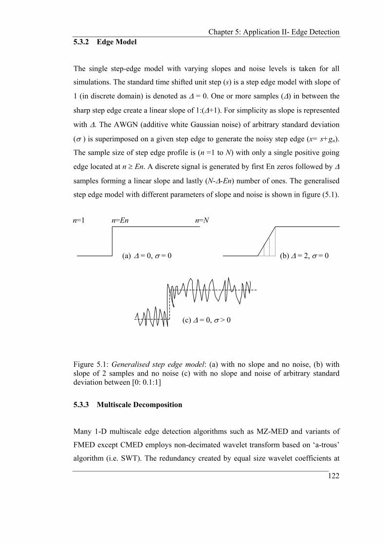
Chapter 5: Application II- Edge Detection 5.3.2 Edge Model
The single step-edge model with varying slopes and noise levels is taken for all
simulations. The standard time shifted unit step (s) is a step edge model with slope of
1 (in discrete domain) is denoted as ∆ = 0. One or more samples (∆) in between the
sharp step edge create a linear slope of 1:(∆+1). For simplicity as slope is represented
with ∆. The AWGN (additive white Gaussian noise) of arbitrary standard deviation
(σ ) is superimposed on a given step edge to generate the noisy step edge (x= s+gn).
The sample size of step edge profile is (n =1 to N) with only a single positive going
edge located at n ≥ En. A discrete signal is generated by first En zeros followed by ∆
samples forming a linear slope and lastly (N-∆-En) number of ones. The generalised
step edge model with different parameters of slope and noise is shown in figure (5.1).
(b) ∆ = 2, σ = 0
(c) ∆ = 0, σ > 0
(a) ∆ = 0, σ = 0
n=1 n=En n=N
Figure 5.1: Generalised step edge model: (a) with no slope and no noise, (b) with slope of 2 samples and no noise (c) with no slope and noise of arbitrary standard deviation between [0: 0.1:1]
5.3.3 Multiscale Decomposition
Many 1-D multiscale edge detection algorithms such as MZ-MED and variants of
FMED except CMED employs non-decimated wavelet transform based on ‘a-trous’
algorithm (i.e. SWT). The redundancy created by equal size wavelet coefficients at
122

Chapter 5: Application II- Edge Detection all levels is important for correct detection and localisation of the step edge without
any loss of information.
Using SWT, N point edge profile is decomposed up to J=log2(N) levels. The
filterbank implementation of classical MZ-MED and standard FMED of uses a
lowpass and highpass filters derived from cubic spline kernel (approximately
Gaussian) and its scale dependent derivatives as shown in figure (5.2).
Figure 5.2: Cubic spline smoothing function φ(t) and its derivative ψ(t) = d/dt(φ(t)). ψj(t)= (1/j)ψ (t/j) is a wavelet yielding a filter bank that estimates the derivative at a level j.
Singularity information at various scales (levels) is used in different ways by
different algorithms to determine the correct edge location.
5.3.4 FMED (Fuzzy Multiscale Edge Detection) Algorithms
Novel implementations of existing standard FMED (Fuzzy Multiscale Edge
Detection) algorithm include FMED (‘db3’), which uses multiscale decomposition
with 6-tap ‘db3’ wavelet, and DB-FMED (Dual-Basis FMED), which uses the
combination of ‘cubic-spline’ scaling kernel and ‘db3’. The implementation steps for
all FMED based algorithms are described as:
1. Non-decimated WT is computed for edge profile x using SWT (Matlab
function swt) up to j = 1 to J=log2(N) levels. FMED (‘cubic’) uses cubic
spline scaling kernel, FMED (‘db3’) uses wavelet basis ‘db3’ for J level
123

Chapter 5: Application II- Edge Detection decomposition while DB-FMED uses two parallel SWT decomposition trees,
one with ‘db3’ and other with ‘cubic spline’ kernel. For cubic spline
implementation, lowpass filter taken is h0 = [1,4,6,4,1]/16 and other analysis
and synthesis filters are computed with matlab function ‘orthfilt’.
w(j,n) = WT(x(n)), j =1 to J, n= 1 to N
2. For DB-FMED, coefficients of both trees at each level are combined with
wavelet fusion averaging rule resulting in only one decomposition tree.
w(j,n)= average{w(j,n)(‘db3’) + w(j,n)(‘cubic spline’)}
3. Depending on size of edge profile (x), slope, and on the wavelet basis
selection, there is a localisation error (in terms of samples) of true edge from
fine to course level in multiscale propagation. This error is reduced with
predetermined offset (± noff) by proper amount and in correct direction (+ for
right and - for left) through cyclic shift of wavelet coefficients at each level.
wo(j,n) = offset { w(j,n), ± noff }
In simulations the relevant offsets for all J levels are selected as:
FMED(‘cubic spline’): noff = 0 (∆ =0) and noff = -(∆-1) (∆>0)
FMED(‘db3’): noff = -(∆-2) (for all ∆>=0)
DB-FMED: noff = +1 (∆ =0) and noff = -(∆-2) (∆>0)
Wavelet coefficients at each level (scale) are zero clipped w+ such that only
positive coefficients are selected for positive going edge model (considered
as per figure (5.1)) and negative w- coefficients if negative going edge model
is considered.
w+ (j,n) = +Ve_clip{wo(j,n)}, w- (j,n) = -Ve_clip{wo(j,n)}
124

Chapter 5: Application II- Edge Detection 4. Coefficients at each level are normalised between [0,1] to be consistent with
fuzzy membership axioms and set operations [178]. Now wavelet coefficients
at each level j can be viewed as fuzzy subset Fj of (µFj(n),n), where µ is the
membership value associated with each of n wavelet coefficients at level j.
Fj = (µFj(n),n) = Normalised {w+ (j,n) or w- (j,n)}
5. Each local maximum of normalised wavelet coefficients (at each level) is a
potential representative of actual step edge in a given signal. Hence at each
scale, a membership value (µFj(n),n) with local maxima (modulus maxima) is
identified and boosted by assigning the highest fuzzy membership value 1.
(µFj(n), n) = 1, if (µFj(n), n) is a local maximum
6. At finer levels the amount of noise is higher and also the chances of false
edge detection are more while at courser levels, the amount of noise is less
but the localisation of true edge is ambiguous. So depending on the edge
location En (in original edge profile) and noise variance, heuristically some
arbitrary number of levels (fuzzy subsets) is selected to compute a minimum
fuzzy set (Fmin) in vertical direction for optimal edge detection.
Fmin = Minimum {Fj} such that
(µFmin(n), n) = Minimum{ (µFj(n), n) }
for j = k1 to k2 ∈ {1 to J}, n= 1 to N
In the presented experiments with FMED algorithms, number of levels
considered are j = 2 to J.
7. The final step of the algorithm is to find the position (index) of a sample
having maximum membership value (horizontal operation) from the
computed minimum fuzzy set (Fmin). The detected position (index) reveals
the true position of an edge in a given noisy edge profile.
125
Chapter 5: Application II- Edge Detection Detected Edge (Dn) = Position{Maximum{ Fmin }}
8. Performance of FMED algorithm is judged by minimisation of RMSE
between the true edge En and detected edge Dn.
5.3.5 CMED (Complex Multiscale Edge Detection) Algorithms
Basic CMED (Complex Multiscale Edge Detection) algorithm is based on redundant
CWT using DT-DWT(K) to exploit the limited redundancy with improved denoising
ability for 1-D edge detection. DT-DWT(K) is a kind of two standard DWT trees
working in parallel, so at each subsequent decomposition there is a data size
reduction by a factor of 2.
Due to quadrature nature of DT-DWT(K), the wavelet coefficients of two trees
pick up the same singularity with some offset and polarity inversion between
respective real and imaginary levels. The novelty of the CMED algorithm is in the
proper alignment of wavelet coefficients of both real and imaginary trees from fine to
course level for efficient edge detection under noisy conditions.
The key steps of basic CMED algorithm are as follows:
1. A given noisy single step-edge profile (x) is decomposed using multi-scale
DT DWT(K) up to J levels in two trees.
2. To compensate for offset and polarity discrepancies, real-tree coefficients are
left shifted (cyclically) by 1-sample (noff = -1) for all levels (j = 1 to J) and
polarity of real-tree coefficients are reverses (for j = 2 to J).
3. For maintaining the same size of coefficients at all levels, both real and
imaginary trees coefficients are interpolated with right amount of level
dependent zeros (2j-1) at each level (j = 1 to J) before each coefficient.
126

Chapter 5: Application II- Edge Detection 4. All coefficients at each level of both trees are zero clipped (keeping only +ve
values) to account for positive going edge.
5. All the coefficients are normalised between [0,1].
6. Coefficients of both real and imaginary trees at each level are combined using
the formula of complex magnitude and phase. The magnitude tree is used for
further processing.
7. Depending on the true location of edge, optimum level jopt = log2(En) is
selected for edge detection with minimum RMSE.
8. The position of maximum magnitude coefficient at a selected optimum level
gives the location of detected edge.
The basic CMED algorithm is not fuzzy based and it works only at a unique level
for optimum edge detection using combined real and imaginary trees. Variants of
CMED algorithm such as CMED algorithm with only imaginary tree (IMED), and
CMED algorithm with fuzzy union of various scales are also investigated (FCMED).
The other variant of CMED namely SFCMED (Spatial Fuzzy CMED) is also
explored through fuzzy combination of reconstructions (of decimated coefficients) at
different scales in spatial domain.
5.3.6 Performance Measure
Root Mean Square Error (RMSE) and percentage Hit (% Hit) are taken for
evaluating the performance of single positive going step edge with different slope
conditions (∆) under varying degree of SNR. Related definitions and equations are
given as:
RMSE (in terms of samples) = 2)( EnEd − (5.1)
where, Ed = Position of detected edge, En = Position of correct edge
127

Chapter 5: Application II- Edge Detection The percentage Hit is defined in two forms, first is percentage Accurate Hit
(%AHit) that is the percentage of detected edge Ed exactly at the true edge location
En (detected without noise), and the second form is percentage Interval Hit (%IHit)
that is the percentage of detected edge Ed within [En-1 to En+∆+1], in the portion of
transition of step edge profile. In other words,
%AHit Ed at En (where En is dependent on basis function and slope) and
%IHit Ed is within [En-1 to En+∆+1] samples. (5.2)
SNR(dB) = 10 log10{ }
−2
2)(σ
ssE (5.3)
where, E(⋅) is an expectation operation, s is an original single step-edge profile with-
out noise, s is the mean value of signal s, and σ 2 is the variance of AWGN super
imposed on signal s.
Slope (∆) = number of samples within the transition of step-edge profile. (5.4)
5.3.7 Results and Discussion
The results of MZ-MED and FWOMED are taken from [177], results of FMED
(‘cubic’) are taken from an individual implementation of the standard FMED
algorithm developed in [176]. Other novel implementations of standard FMED with
different basis such as FMED(‘db3’) and DB-FMED are developed individually
during the studies of standard FMED. An original CMED algorithm is developed
using DT-DWT(K). A quantitative comparison of various algorithms for a selected
step-edge profile, with different parameters is given in tables (5.1) to (5.5), uniformly
iterated 50, 000 times for all algorithms using Monte-Carlo simulations.
Implementation of FMED (‘cubic’) for a noisy and sloppy single edge step-
edge profile (with nearly accurate detection of the edge as a result) is shown in figure
(5.3). Wavelet coefficients at J levels and their zero clipped +ve parts are shown in
figure (5.4). J level fuzzy subsets of clipped coefficients and their interactions (at 128

Chapter 5: Application II- Edge Detection level 2 to J) to form a minimum fuzzy set are shown in figure (5.5). Processing steps
related to basic CMED algorithm are highlighted through figures (5.6) to (5.10).
From the results in tables (5.1) to (5.5), it can be concluded that for all noise
and slope conditions, the FWOMED algorithm is better than well known MZ-MED
algorithm and FMED (‘cubic’) algorithm in terms of RMSE error. Two FMED based
algorithms namely FMED (‘db3’) and DB-FMED perform better than all other non-
decimated multiscale edge detection algorithms in varying slope and noise
conditions. Performance of FMED (‘db3’) is optimum in lower slope conditions (∆
=0,1), where as DB-FMED is optimum for moderate to higher slope conditions (∆
=3,5). Basic CMED algorithm is comparable to other FMED algorithms in lower
noise conditions (σ ≤ 0.4) for all slope conditions.
CMED algorithm is significantly poorer in higher noise conditions. Also the
other major disadvantage of basic CMED algorithm is its limitation to detect the
edges located only at power of two indices. The other variants such as IMED,
FCMED and SFCMED are even poorer than basic CMED. The limitations of basic
CMED algorithm are because of the use of decimated DT-DWT(K) and single level
detection strategy. But the promising %Hit results (table 5.5) with accurate
localisation of edge at courser levels (at level 4 and 5 in figure (5.9)) with DT-
DWT(K) suggest its potential for further investigations to generalise the basic
CMED algorithm.
It is proposed that by developing new non-decimated version of DT-DWT(K)
with multilevel fuzzy reasoning might generalise a basic CMED to NFCMED (Non-
decimated Fuzzy CMED) for detection of any arbitrary edge (not exactly at power of
2 locations). NFCMED being equally redundant at all levels and having all the
benefits of CWT might prove to be a challenging research for comparable
performance against the variants of FMED algorithms.
129
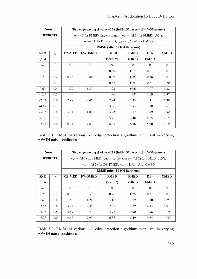
Chapter 5: Application II- Edge Detection
Step edge having ∆ =0, N =128 (initial 32 zeros + ∆ + N-32-∆ ones)
noff = 0 for FMED(‘cubic_spline’), noff = -(∆-2) for FMED(‘db3’),
noff = +1 for DB-FMED, noff = -1, jopt =5 for CMED
Noise
Parameters
RMSE (after 50 000 iterations)
SNR
(dB)
σ MZ-MED FWOMED FMED
(‘cubic’)
FMED
(‘db3’)
DB-
FMED
CMED
∞ 0 0 0 0 0 0 0
12.73 0.1 0.30 0.17 0.21 0
6.71 0.2 0.26 0.86 0.48 0.35 0.38 0
3.19 0.3 0.67 0.65 0.61 0.20
0.69 0.4 1.29 1.33 1.23 0.96 1.07 1.32
-1.25 0.5 1.96 1.68 1.69 3.37
-2.83 0.6 2.98 2.45 2.94 2.35 2.41 6.30
-4.17 0.7 3.86 2.93 3.18 8.63
-5.33 0.8 5.81 4.83 5.23 3.82 3.99 10.65
-6.35 0.9 5.71 4.48 4.85 12.79
-7.27 1.0 9.31 7.83 6.45 5.36 5.70 14.48
Table 5.1: RMSE of various 1-D edge detection algorithms with ∆=0 in varying AWGN noise conditions.
Step edge having ∆ =1, N =128 (initial 32 zeros + ∆ + N-32-∆ ones)
noff = -(∆-1) for FMED(‘cubic_spline’), noff = -(∆-2) for FMED(‘db3’),
noff = -(∆-2) for DB-FMED, noff = -1, jopt =5 for CMED
Noise
Parameters
RMSE (after 50 000 iterations)
SNR
(dB)
σ MZ-MED FWOMED FMED
(‘cubic’)
FMED
(‘db3’)
DB-
FMED
CMED
∞ 0 0 0 0 0 0 0
6.71 0.2 0.75 0.57 0.26 0.25 0.31 0.01
0.69 0.4 1.56 1.24 1.16 1.09 1.10 1.25
-2.83 0.6 3.27 2.44 2.86 2.39 2.44 6.07
-5.33 0.8 5.89 4.73 4.76 3.90 3.98 10.78
-7.27 1.0 9.67 7.93 6.37 5.49 5.64 14.40
Table 5.2: RMSE of various 1-D edge detection algorithms with ∆=1 in varying AWGN noise conditions. 130
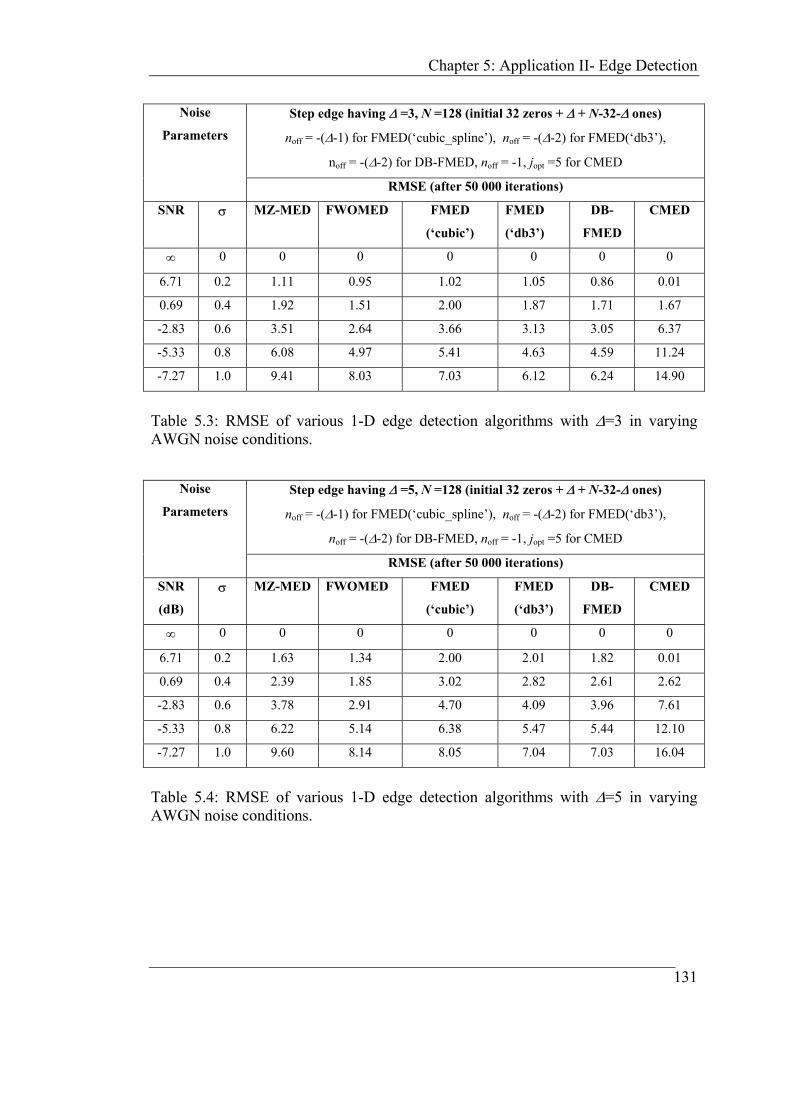
Chapter 5: Application II- Edge Detection
Step edge having ∆ =3, N =128 (initial 32 zeros + ∆ + N-32-∆ ones)
noff = -(∆-1) for FMED(‘cubic_spline’), noff = -(∆-2) for FMED(‘db3’),
noff = -(∆-2) for DB-FMED, noff = -1, jopt =5 for CMED
Noise
Parameters
RMSE (after 50 000 iterations)
SNR σ MZ-MED FWOMED FMED
(‘cubic’)
FMED
(‘db3’)
DB-
FMED
CMED
∞ 0 0 0 0 0 0 0
6.71 0.2 1.11 0.95 1.02 1.05 0.86 0.01
0.69 0.4 1.92 1.51 2.00 1.87 1.71 1.67
-2.83 0.6 3.51 2.64 3.66 3.13 3.05 6.37
-5.33 0.8 6.08 4.97 5.41 4.63 4.59 11.24
-7.27 1.0 9.41 8.03 7.03 6.12 6.24 14.90
Table 5.3: RMSE of various 1-D edge detection algorithms with ∆=3 in varying AWGN noise conditions.
Step edge having ∆ =5, N =128 (initial 32 zeros + ∆ + N-32-∆ ones)
noff = -(∆-1) for FMED(‘cubic_spline’), noff = -(∆-2) for FMED(‘db3’),
noff = -(∆-2) for DB-FMED, noff = -1, jopt =5 for CMED
Noise
Parameters
RMSE (after 50 000 iterations)
SNR
(dB)
σ MZ-MED FWOMED FMED
(‘cubic’)
FMED
(‘db3’)
DB-
FMED
CMED
∞ 0 0 0 0 0 0 0
6.71 0.2 1.63 1.34 2.00 2.01 1.82 0.01
0.69 0.4 2.39 1.85 3.02 2.82 2.61 2.62
-2.83 0.6 3.78 2.91 4.70 4.09 3.96 7.61
-5.33 0.8 6.22 5.14 6.38 5.47 5.44 12.10
-7.27 1.0 9.60 8.14 8.05 7.04 7.03 16.04
Table 5.4: RMSE of various 1-D edge detection algorithms with ∆=5 in varying AWGN noise conditions.
131

Chapter 5: Application II- Edge Detection
Step edge having N =128 (initial 32 zeros + ∆ + N-32-∆ ones) Noise
and
Slope % AHit (after 50 000 iterations) % IHit (after 50 000 iterations)
σ ∆ FMED
(‘cubic’)
FMED
(‘db3’)
DB-
FMED
CMED
FMED
(‘cubic’)
FMED
(‘db3’)
DB-
FMED
CMED
0 100 100 100 100 100 100 100 100
1 100 100 100 100 100 100 100 100
3 100 100 100 100 100 100 100 100 0
5 100 100 100 100 100 100 100 100
0 54 67 63 100 100 98 100 100
1 76 78 71 99 98 99 98 99
3 32 30 39 99 99 99 100 99 0.2
5 17 15 18 99 99 100 100 99
0 38 48 41 98 83 82 88 98
1 46 46 46 98 81 85 84 98
3 20 20 25 97 88 93 94 97 0.4
5 12 12 13 96 89 93 93 96
0 25 33 27 89 61 63 70 89
1 29 29 30 90 59 67 67 90
3 14 15 16 89 72 80 81 89 0.6
5 8 9 10 87 74 82 83 87
0 17 23 19 81 44 59 54 81
1 19 20 21 81 44 53 53 81
3 10 11 12 80 59 68 69 80 0.8
5 7 7 8 79 63 71 72 79
0 13 17 14 73 34 38 44 73
1 14 16 15 74 34 44 43 74
3 8 9 10 73 48 58 58 73 1.0
5 6 6 7 71 54 62 62 71
Table 5.5: % Hit of various 1-D edge detection algorithms in varying slope and AWGN noise conditions.
132

Chapter 5: Application II- Edge Detection
Figure 5.3: 1-D edge detection with FMED (‘cubic’) with σ =0.6 and ∆=5.
Figure 5.4: J level wavelet coefficients (left) and their only positive parts (right) with FMED(‘cubic’) under the noise of σ =0.6 and slope of ∆=5. 133

Chapter 5: Application II- Edge Detection
Figure 5.5: J level fuzzy subsets (left) and their corresponding 2 to J level fuzzy intersection (right) for the computation of minimum fuzzy set (right top) employing FMED (‘cubic’) under the noise of σ =0.6 and slope of ∆=5
Figure 5.6: 1-D edge detection with CMED: σ =0.6 and ∆=5
134
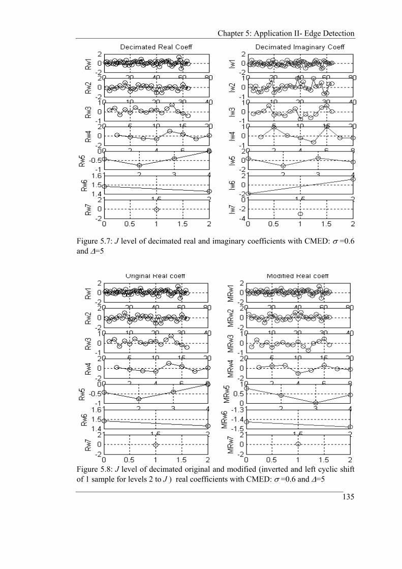
Chapter 5: Application II- Edge Detection
Figure 5.7: J level of decimated real and imaginary coefficients with CMED: σ =0.6 and ∆=5
Figure 5.8: J level of decimated original and modified (inverted and left cyclic shift of 1 sample for levels 2 to J ) real coefficients with CMED: σ =0.6 and ∆=5
135

Chapter 5: Application II- Edge Detection
Figure 5.9: J level of interpolated modified real and original imaginary coefficients with CMED: σ =0.6 and ∆=5
Figure 5.10: J level of complex magnitude coefficients (left) and fuzzy subsets of complex magnitudes (right). Top left shows detected edge with complex magnitude (at level 5) and top right shows detected edge with fuzzy subset (at level 5) employing CMED: σ =0.6 and ∆=5 136

Chapter 5: Application II- Edge Detection 5.4 2-D Edge Detection
As discussed in the introduction of section 5.1, edge information is very precious for
various image-processing applications. Review of many conventional algorithms and
methods based on edge detection for image processing can be found in [179-181].
Though Canny’s operator is a robust edge detector in a noisy environment [161],
some less noticed and unconventional methods for edge in noisy conditions can be
found in [182,183].
5.4.1 Basic Approach
Multiscale methods based on non-orthogonal (and redundant) wavelet transform
[163,164] showed promising performance for edge detection in noisy environment,
and are widely employed in many applications. Object segmentation, Motion
estimation, Image fusion, Image registration and CBIR (Content Based Image
Retrieval) are just a few examples utilising the multiscale edge information for image
processing [184-190]. More recently many researchers have combined advanced
techniques such as Fuzzy reasoning [191-193], HMM (Hidden Markov Models)
[194,195], Neural networks [196,197], and Genetic algorithms [198] for improved
multiscale image segmentation, registration and object extraction in wide range of
applications.
Though redundancy and Gaussian like wavelet basis are common in many
multiscale edge-detection applications, viewpoint of our research is different for 2-D
edge detection. Central theme of this research is to investigate the effects of
redundancy, shift-invariance and directionality of different types of wavelet
transforms in edge detection. In this section, 2-D edge detection is investigated using
various wavelet based, and conventional algorithms. 2-D separable wavelet-based
algorithms employ standard DWT, SWT and redundant CWT (namely DT-DWT(K)
and DT-DWT(S)), whereas conventional algorithms are based on 2-D edge operators
such as Prewitt, Sobel, and Canny.
137
Chapter 5: Application II- Edge Detection 5.4.2 Algorithms
5.4.2.1 WT based Algorithm
2. The lowpass subband is filled with zeros and all high-pass subbands are
unchanged.
3. A J level reconstruction is performed with relevant inverse wavelet
transform.
4. From recovered image, 2-D edge thinning mask is computed using local
maxima approach.
5. The recovered image is thresholded by a suitable heuristic threshold to
eliminate features below certain intensities.
6. Final edge detection is achieved by multiplying the thresholded image with
thinning mask.
5.4.2.2 CWT based Algorithm
With DT-DWT(K) and DT-DWT(S)
1. An image (of size in power of 2 in both directions) is taken.
Conventional 2-D edge detection is performed using Matlab (image processing
toolbox) function ‘edge’ with default settings. The wavelet-based algorithms employ
a simple strategy (without any advanced optimisation techniques to combat with
noise) to verify the subtle differences of edge detection performance of various
wavelet transforms.
With standard DWT and SWT
1. A given image (2-D signal) is decomposed to J levels using standard DWT or
SWT with suitable wavelet basis.
138

Chapter 5: Application II- Edge Detection 2. The image is decomposed with the redundant CWT (using DT-DWT(K) or
DT-DWT(S)) to the depth of J levels.
3. All lowpass subbands (four) of last levels are set to zeros.
4. Any highpass subbands of real or imaginary trees are not altered
5. J level inverse transform is taken to reconstruct the image.
6. A 2-D thinning mask from reconstructed image is computed by finding local
maximum (horizontal and vertical). Comparative neighbour-hood approach is
used to form this mask.
7. Reconstructed image is thresholded with heuristic threshold value using hard
or soft thresholding to form a binary image.
8. A refined image with sharp edges is obtained by multiply a thinning mask
with binary output image.
5.4.3 Performance Measure
In general it is quite challenging to compare the performance of edge detection
algorithms in quantitative manner. Even though the definition of edge is also difficult
to quantify objectively, there are a few proposed measure to quantify the
performance of edge detectors such as conditional probabilities P(ntnd ), P(
ntnd ),
MSD (Mean Squared Distance) and FOM (Figure of Merit) as suggested in
[199,200].
MSD = ∑=
nd
idi
nd 1
21
FOM = ∑= +
nd
i dintnd 129.01
1},max{
1 (5.5)
139

Chapter 5: Application II- Edge Detection where, nd = no. of detected edge pixels, nt = no. of true edge pixels, di = edge
deviation of ith detected pixel from its true position.
These quantitative measures may be reasonable for predetermined and simple
test images but not practical for natural images, and are not widely used. Hence in
this research, the results are presented for qualitative comparisons relying on the
human visual system.
5.4.4 Results and Discussion
The results of various edge detectors for a test image are shown in figures (5.11) and
(5.12).
Original
50 100 150 200 250
50
100
150
200
250
Sobel
50 100 150 200 250
50
100
150
200
250
Prewitt
50 100 150 200 250
50
100
150
200
250
Canny
50 100 150 200 250
50
100
150
200
250
Figure 5.11: 2-D edge detection with conventional edge operators
140

Chapter 5: Application II- Edge Detection
Standard DWT
50 100 150 200 250
50
100
150
200
250
SWT
50 100 150 200 250
50
100
150
200
250
DT-DWT(S)
50 100 150 200 250
50
100
150
200
250
DT-DWT(K)
50 100 150 200 250
50
100
150
200
250
Figure 5.12: 2-D edge detection with wavelet based methods. For all method, test image is 256×256 ‘ring.jpg’, J =2 and threshold value = 35. For standard DWT and SWT wavelet basis is ‘db2’. The wavelet filters used for DT-DWT(K) are ‘near_sym_b’ and ‘qshift_b’ as given in appendix A and the filters for DT-DWT(S) are as given is appendix B.
From the figures (5.11) and (5.12), it is clear that conventional 2-D edge
detectors (of matlab) with default thresholding schemes are better than simple
implementation of wavelet based detectors for detection boundaries with very good
sharpness and resolutions without noise as well and in noisy conditions. Canny edge
detector with its defaults settings is more liberal (and more leaky) than Prewitt and
Sobel but flexibility makes it more robust in blurred images.
141
The results in figure (5.12) show that the performance of both DT-DWT
methods is superior to the standard DWT due to its (4:1) redundancy, and improved
directionality (with more spatial orientations). The superior performance of SWT
Chapter 5: Application II- Edge Detection compared to standard DWT lies in its highly redundant representation. Visually,
performance of SWT is comparable to both DT-DWTs. The results presented here
are without the presence of noise.
A set of experiments show that the redundancy is of prime importance for
improved edge detection in wavelet domain. Improved directionality also plays an
important role in images with large number of randomly oriented edges. More
sophisticated techniques may be employed in wavelet domain to combat with noise
utilizing the directionality and/or redundancy of the transforms for improvement over
conventional edge detectors.
5.5 Conclusion
It is concluded that redundancy of the transform is very important for efficient Edge
detection with multiscale approaches. Directionality of the transform also plays an
important role in fidelity of Edge detection in multi dimensions.
Multiscale algorithms (FMED extensions) with non-decimated SWT having
Gaussian like kernel are promising for single edge, 1-D Edge detection in higher
noise environment over other classical Edge detection approaches (Canny, Prewitt
etc.). Limited redundant DT-DWT, being a decimated extension, is not very
promising for 1-D Edge detection in its original form with CMED. The accuracy of
edge localisation at lower resolution scales is higher with DT-DWT (using CMED
algorithm) than with SWT (using FMED algorithms) suggests it potential for further
investigations using its non-decimated extension.
For 2-D Edge detection, performance of DT-DWT is superior to standard
DWT but almost similar to SWT. Integration of advanced noise removal, and multi-
edge detection techniques with non-decimated DT-DWT might be suitable for
efficient Edge detection in images corrupted by higher noise.
142

Chapter 6: Conclusions and Future Scope
Chapter 6:
Conclusions and Future Scope
6.1 Conclusions
In this thesis, Wavelet Transforms (WT) is reviewed in detail. The history, evolution,
and various forms of WTs are investigated. Advantages, applications, and limitations
of popular standard DWT and its extensions are realised. Complex Wavelet
Transforms (CWT), a powerful extension to real valued WT is thoroughly
investigated to reduce the major limitations of standard DWT and its extensions in
certain signal processing applications.
The history, basic theory, recent trends, and various forms of CWTs with
their applications are collectively and comprehensively analysed. Recent
developments in CWTs are critically compared with existing forms of WTs.
Potential applications are investigated and suggested that can be benefited with the
use of different variants of CWTs.
143
Individual software codes are developed for simulation of selected
applications such as Denoising and Edge detection using both WTs and CWTs. The
performance is statistically validated and compared to determine the advantages and
limitations of CWTs over well-established WTs. Promising results are obtained using
individual implementation of existing algorithms incorporating novel ideas into well-
established frameworks.

Chapter 6: Conclusions and Future Scope In chapter 2, the background for analysing the CWTs is presented. WTs are
reviewed in detail with individual investigations and simulations. Complex
mathematical formulations and important properties of WTs are studied. Evolution
and advantages of WTs as an alternative to FT for non-stationary signals are studied.
1-D and 2-D implementations of various versions of WTs are realised with software
simulations. Applications of various forms of WTs are surveyed. It is realised that
WT is an important tool for non-stationary signal processing applications. WT has a
great potential for singularity detection, denoising and compression and it presents a
novel framework of time-scale for analysing and characterising many natural signals
with the wealth of time-varying information. Chapter 2 concludes with three major
disadvantages of widely used standard DWT, namely; Shift-sensitivity, Poor-
directionality, and Lack of Phase-information. These disadvantages severely limit the
applications of WTs in certain signal processing applications. It ends with motivation
to reduce these disadvantages of WTs through a complex extension known as CWTs.
Thorough analysis of CWTs is presented in chapter 3. The limitations of the
earlier work on CWTs (with the motivation to utilise both the magnitude and phase
information in more effective manner than real valued WTs) are presented. Recent
developments in the field of CWTs, with the motivation to reduce all three
limitations of standard DWT, are critically analysed. CWTs are classified into two
important categories namely RCWT (Redundant CWT) and NRCWT (Non-
redundant CWT). RCWT include DT-DWT(S) (Selesnick’s Dual-Tree DWT) and
DT-DWT(K) (Kingsbury’s Dual-Tree DWT). Theory, filterbank structure and
properties of both DT-DWTs are critically investigated and compared. Similarly for
NRCWT, Fernandes’s PCWT (Projection based CWT), and Spaendonck’s non-
redundant OHCWT (Orthogonal Hilbert Transform filterbank based CWT) are
investigated.
Implementation for both DT-DWTs and PCWT is realised through Matlab
simulations based on the theories of sections 3.5 and 3.5. Comparative summary of
all CWTs are presented in table (3.2). Depending upon the redundancy and
properties, potential applications are suggested (based on literature review, thorough
144

Chapter 6: Conclusions and Future Scope investigations, and after primary level implementations) that can be benefited by
further investigations with various forms of CWTs as an alternative to existing DWT
extensions.
In chapter 4, individual implementations of WTs and CWTs (explicitly DT-
DWTs) with Matlab simulations are presented for an important signal/image
processing application namely Denoising. In chapter 4, 1-D and 2-D CWTs are
implemented for signals and images in exiting framework of wavelet shrinkage
denoising algorithms. Some novel modifications are made in threshold selections and
thresholding strategies. The results are compared with variants of WT based
algorithms and other conventional filtering techniques such as Mean, Median and
Wiener Filtering. It is observed that in general for higher noise environment, CWTs
perform better than WTs and other conventional techniques for different 1-D and 2-
D signals. Effects of number of wavelet parameters are investigated. 1-D CWTs are
also investigated with certain novel ideas for audio denoising (with initially poor
SNR), producing some promising results over standard DWT.
In chapter 5, for Edge Detection application, the background research in the
Signal Processing Group of University of Strathclyde is explored further with the
novel ideas in existing frameworks. The existing WT based 1-D edge-detection
algorithms such as MZ-MED, FMED and FWOMED are reviewed. Individual
implementation of cubic spline base FMED algorithm culminated in newer FMED
(‘db3’) and DB-FMED algorithms with their novel implementation using different
bases. The newer algorithms showed an improved performance over both FMED and
FWOMED in higher noise and slope conditions. Experiments with CWT for 1-D
edge detection resulted in a basic CMED algorithm. CMED algorithm is still in its
primary stage, with promising edge localisation property at lower resolution scales,
compared to other WT based multiscale algorithms. For 2-D edge detection, a very
basic strategy of neglecting the lowpass subband is applied to investigate the
advantage of CWT over standard DWT. Other conventional edge detectors such as
Prewitt and Canny are also implemented for comparison. The result of 2-D edge
detection shows the improved performance of CWTs over standard DWT because of
145

Chapter 6: Conclusions and Future Scope its improved directionality and limited redundancy. The performance of redundant
WT (i.e. SWT) compared to DT-DWT based CWT suggests the importance of higher
redundancy in edge detection.
6.2 Future Scope
It is concluded that CWT (having separable implementation, perfect
reconstruction, limited (or no) redundancy, and improved properties over real-valued
WTs) has a potential for many signal and image processing applications yet to be
explored.
Due to limited academic time span, NRCWT such as Fernandes’s PCWT and
Spaendonck’s OHCWT have yet to be explored for denoising applications. It is
assumed that the properties of PCWT-CR similar to DT-DWTs will result in a
comparable performance. Even non-decimated DT-DWTs might even improve the
denoising performance over existing DT-DWTs.
The initial simulations for 1-D edge detection show potential scope of further
investigation to enhance basic CMED algorithm in higher noise conditions. The
suggested NFCMED (Non-decimated Fuzzy CMED) algorithm should be explored
for improved 1-D edge detection in higher noise conditions. The extension of
NFCMED in 2-D incorporating multiple edge detection and other techniques suitable
for higher noise might yield a robust and optimum algorithm for object extraction
and segmentation from noisy video clips. Fernandes’s PCWT with redundant
projections (PCWT-CR) should also be explored in similar manner that gives fully
redundant projection based CWT suitable for edge detection applications.
DT-DWTs with their good shift invariance should be considered for potential
investigations in applications such as Motion estimation in video coding, SAR
remote sensing, Texture segmentation, and Image fusion. The non-redundant
NRCWT (explicitly PCWT-NR and OHCWT) has a strong potential for further
146

Chapter 6: Conclusions and Future Scope investigations in directional compression leading toward an improved moderate to
low bit-rate video codecs.
Potential applications for further investigations with CWTs are summarised
in table (3.2). There is also a potential challenge for improvement in filter designs to
further minimising the aliasing of subbands for immunity towards shift-sensitivity,
and merging the standard DWT strategies to add two more orientations at 0° and 90°
to the available orientations of CWT for further improved directionality. Many
researchers perceived that though wavelets showed tremendous applications in signal
processing, they are still not optimum in dealing with sparse singularises in natural
images. Curvelets, Contourlets, and Piecewise approximations are the newer basis
emerging beyond wavelets. It would be interesting to explore the possibility of
similar complex extensions to such newer basis and analyse their properties in signal
processing context.
147

Appendices
Appendix A Filters used to implement DT-DWT(K) uses Kingsbury’s Dual-Tree Complex
Wavelet Transform available from: [email protected] ,
http://www-sigproc.eng.cam.ac.uk/~ngk/
First stage Filters:
Antonini, Legall, near_sym_a and near_sym_b.
Q-shift Filters (after first stage):
qshift_06, qshift_a, qshift_b, qshift_c, and qshift_d.
For example ‘near_sym_b’ filters:
Real-tree Analysis Filter Lowpass Filter (h0) Highpass Filter (h1) 1 -0.00175781250000 -0.00007062639509 2 0 0 3 0.02226562500000 0.00134190150670 4 -0.04687500000000 -0.00188337053571 5 -0.04824218750000 -0.00715680803571 6 0.29687500000000 0.02385602678571 7 0.55546875000000 0.05564313616071 8 0.29687500000000 -0.05168805803571 9 -0.04824218750000 -0.29975760323661 10 -0.04687500000000 0.55943080357143 11 0.02226562500000 -0.29975760323661 12 0 -0.05168805803571 13 -0.00175781250000 0.05564313616071 14 0.02385602678571 15 -0.00715680803571 16 -0.00188337053571 17 0.00134190150670 18 0 19 -0.00007062639509
Table (A1): First stage filters (for near_sym_b): Imaginary-tree analysis filters are one sample delayed than the real-tree filters. Synthesis filters are obtained by negating odd-indexed coefficients and swapping bands.
148
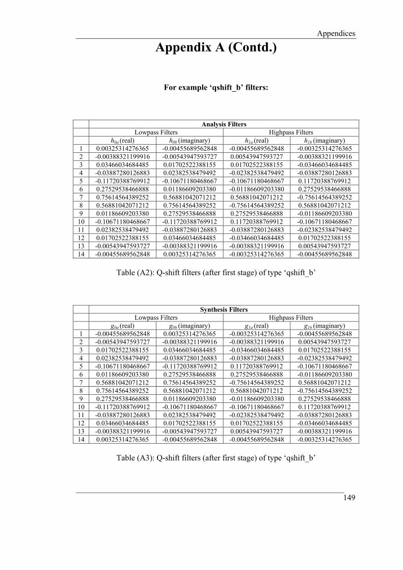
Appendices
Appendix A (Contd.)
For example ‘qshift_b’ filters:
Analysis Filters Lowpass Filters Highpass Filters h0a (real) h0b (imaginary) h1a (real) h1b (imaginary)
1 0.00325314276365 -0.00455689562848 -0.00455689562848 -0.00325314276365 2 -0.00388321199916 -0.00543947593727 0.00543947593727 -0.00388321199916 3 0.03466034684485 0.01702522388155 0.01702522388155 -0.03466034684485 4 -0.03887280126883 0.02382538479492 -0.02382538479492 -0.03887280126883 5 -0.11720388769912 -0.10671180468667 -0.10671180468667 0.11720388769912 6 0.27529538466888 0.01186609203380 -0.01186609203380 0.27529538466888 7 0.75614564389252 0.56881042071212 0.56881042071212 -0.75614564389252 8 0.56881042071212 0.75614564389252 -0.75614564389252 0.56881042071212 9 0.01186609203380 0.27529538466888 0.27529538466888 -0.01186609203380
10 -0.10671180468667 -0.11720388769912 0.11720388769912 -0.10671180468667 11 0.02382538479492 -0.03887280126883 -0.03887280126883 -0.02382538479492 12 0.01702522388155 0.03466034684485 -0.03466034684485 0.01702522388155 13 -0.00543947593727 -0.00388321199916 -0.00388321199916 0.00543947593727 14 -0.00455689562848 0.00325314276365 -0.00325314276365 -0.00455689562848
Table (A2): Q-shift filters (after first stage) of type ‘qshift_b’
Synthesis Filters Lowpass Filters Highpass Filters g0a (real) g0b (imaginary) g1a (real) g1b (imaginary)
1 -0.00455689562848 0.00325314276365 -0.00325314276365 -0.00455689562848 2 -0.00543947593727 -0.00388321199916 -0.00388321199916 0.00543947593727 3 0.01702522388155 0.03466034684485 -0.03466034684485 0.01702522388155 4 0.02382538479492 -0.03887280126883 -0.03887280126883 -0.02382538479492 5 -0.10671180468667 -0.11720388769912 0.11720388769912 -0.10671180468667 6 0.01186609203380 0.27529538466888 0.27529538466888 -0.01186609203380 7 0.56881042071212 0.75614564389252 -0.75614564389252 0.56881042071212 8 0.75614564389252 0.56881042071212 0.56881042071212 -0.75614564389252 9 0.27529538466888 0.01186609203380 -0.01186609203380 0.27529538466888
10 -0.11720388769912 -0.10671180468667 -0.10671180468667 0.11720388769912 11 -0.03887280126883 0.02382538479492 -0.02382538479492 -0.03887280126883 12 0.03466034684485 0.01702522388155 0.01702522388155 -0.03466034684485 13 -0.00388321199916 -0.00543947593727 0.00543947593727 -0.00388321199916 14 0.00325314276365 -0.00455689562848 -0.00455689562848 -0.00325314276365
Table (A3): Q-shift filters (after first stage) of type ‘qshift_b’
149

Appendices
Appendix B Filters used to implement DT-DWT(S) uses Selesnick’s Dual-Tree DWT available
from: [email protected], http://taco.poly.edu/selesi/
Analysis Filters Real Tree Imaginary Tree Lowpass Highpass Lowpass Highpass
1 0 0 0.01122679215254 0 2 -0.08838834764832 -0.01122679215254 0.01122679215254 0 3 0.08838834764832 0.01122679215254 -0.08838834764832 -0.08838834764832 4 0.69587998903400 0.08838834764832 0.08838834764832 -0.08838834764832 5 0.69587998903400 0.08838834764832 0.69587998903400 0.69587998903400 6 0.08838834764832 -0.69587998903400 0.69587998903400 -0.69587998903400 7 -0.08838834764832 0.69587998903400 0.08838834764832 0.08838834764832 8 0.01122679215254 -0.08838834764832 -0.08838834764832 0.08838834764832 9 0.01122679215254 -0.08838834764832 0 0.01122679215254
10 0 0 0 -0.01122679215254
Table (B1): First stage analysis filters
Synthesis Filters Real Tree Imaginary Tree Lowpass Highpass Lowpass Highpass
1 0 0 0 -0.01122679215254 2 0.01122679215254 -0.08838834764832 0 0.01122679215254 3 0.01122679215254 -0.08838834764832 -0.08838834764832 0.08838834764832 4 -0.08838834764832 0.69587998903400 0.08838834764832 0.08838834764832 5 0.08838834764832 -0.69587998903400 0.69587998903400 -0.69587998903400 6 0.69587998903400 0.08838834764832 0.69587998903400 0.69587998903400 7 0.69587998903400 0.08838834764832 0.08838834764832 -0.08838834764832 8 0.08838834764832 0.01122679215254 -0.08838834764832 -0.08838834764832 9 -0.08838834764832 -0.01122679215254 0.01122679215254 0
10 0 0 0.01122679215254 0
Table (B2): First stage synthesis filters
150
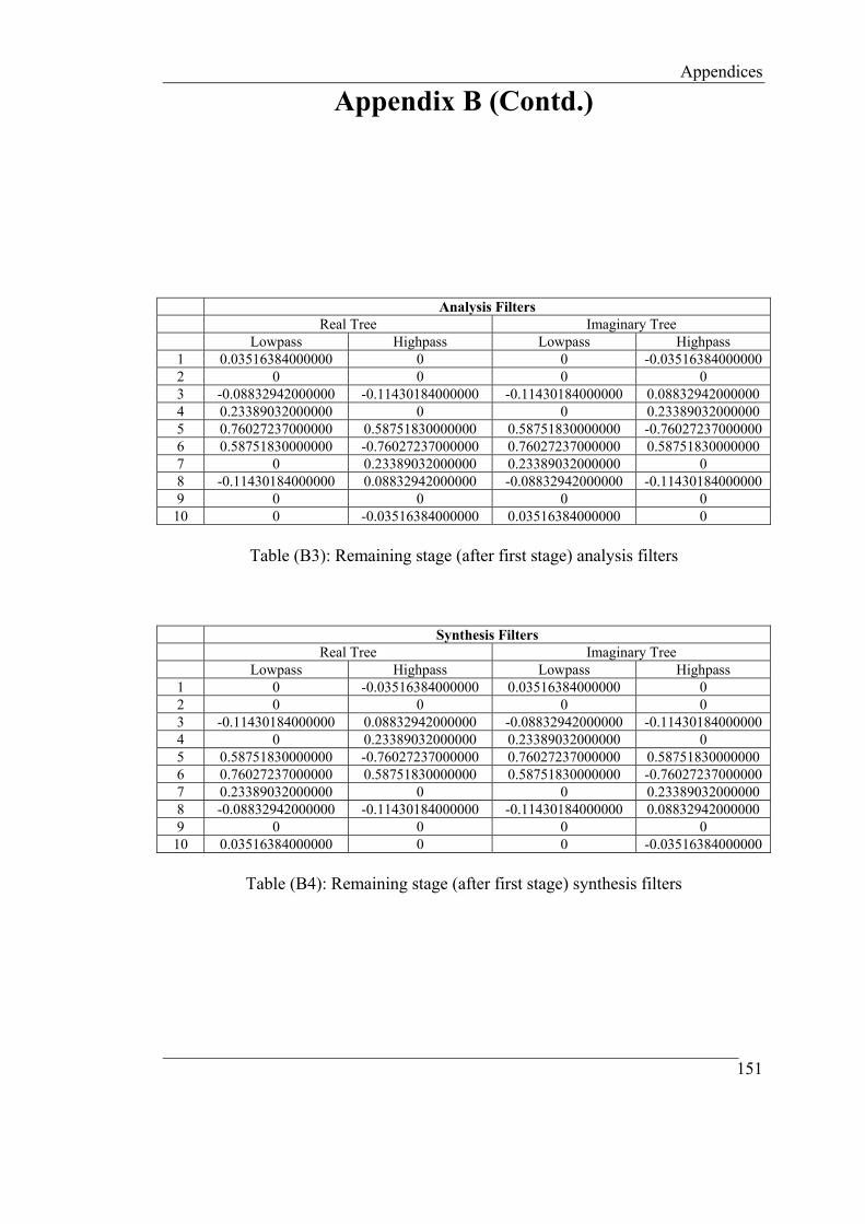
Appendices
Appendix B (Contd.)
Analysis Filters Real Tree Imaginary Tree Lowpass Highpass Lowpass Highpass
1 0.03516384000000 0 0 -0.03516384000000 2 0 0 0 0 3 -0.08832942000000 -0.11430184000000 -0.11430184000000 0.08832942000000 4 0.23389032000000 0 0 0.23389032000000 5 0.76027237000000 0.58751830000000 0.58751830000000 -0.76027237000000 6 0.58751830000000 -0.76027237000000 0.76027237000000 0.58751830000000 7 0 0.23389032000000 0.23389032000000 0 8 -0.11430184000000 0.08832942000000 -0.08832942000000 -0.11430184000000 9 0 0 0 0
10 0 -0.03516384000000 0.03516384000000 0
Table (B3): Remaining stage (after first stage) analysis filters
Synthesis Filters Real Tree Imaginary Tree Lowpass Highpass Lowpass Highpass
1 0 -0.03516384000000 0.03516384000000 0 2 0 0 0 0 3 -0.11430184000000 0.08832942000000 -0.08832942000000 -0.11430184000000 4 0 0.23389032000000 0.23389032000000 0 5 0.58751830000000 -0.76027237000000 0.76027237000000 0.58751830000000 6 0.76027237000000 0.58751830000000 0.58751830000000 -0.76027237000000 7 0.23389032000000 0 0 0.23389032000000 8 -0.08832942000000 -0.11430184000000 -0.11430184000000 0.08832942000000 9 0 0 0 0
10 0.03516384000000 0 0 -0.03516384000000
Table (B4): Remaining stage (after first stage) synthesis filters
151
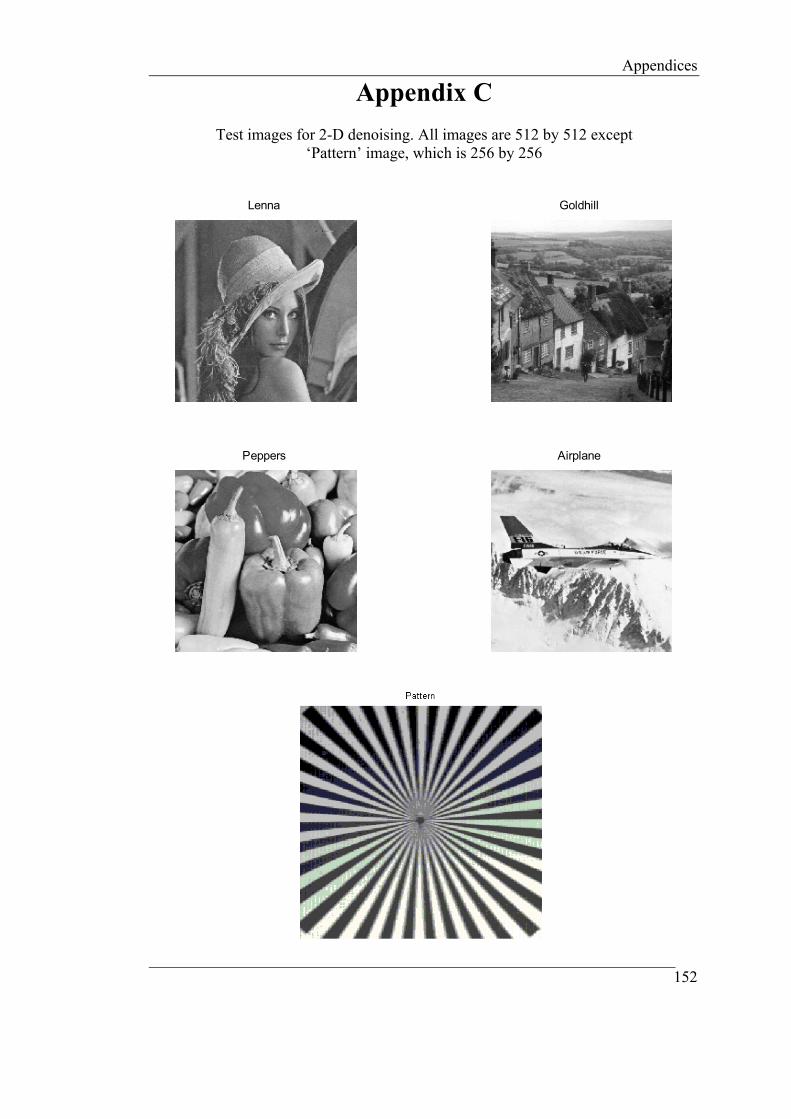
Appendices
Appendix C
Test images for 2-D denoising. All images are 512 by 512 except ‘Pattern’ image, which is 256 by 256
Lenna Goldhill
Peppers Airplane
152

References
References
1 C Sidney Burrus, R A Gopinath, and Haitao Guo, ‘Introduction to Wavelets
and Wavelet Transforms: A Primer’, Prentice Hall, NJ, 1998
2 Stephane Mallat, ‘A Wavelet Tour of Signal Processing’, 2/ed, Academic
Press, 1999
3 J Littlewood, and R Paley, ‘Theorems on Fourier Series and Power Series’,
Proc. London Math. Soc., 42, 52-89, 1937
4 A Calderon, ‘Intermediate Spaces and Interpolation, the Complex Method’,
Studia Math., 24, 113-190, 1964
5 J Morlet et al., ‘Wave Propagation and Sampling Theory’, Geophysics, 47,
203-236, 1982
6 A Grossmann, and J Morlet, ‘ Decomposition of Hardy Functions into Square
Integrable Wavelets of Constant Shape’, SIAM J. Math. Anal., 15, 723-736,
1984
7 Y Meyer, ‘Orthonormal Wavelets’ in Wavelets: Time-Frequency Methods
and Phase Spaces (J M Combes, A Grossmann and Ph Tchamitchian,
editors), 2/ed, Springer Verlag, NY, 21-37, 1989
8 I Daubechies, ‘Where do Wavelets Come From?- A Personal Point of View’,
Proc. IEEE, 84(4), 510-513, 1996
9 Barbara B Hubbard, ‘The World According to Wavelets’, A K Peters Ltd.,
Wellesley, MA, 1996
10 G Strang, ‘Wavelets and Dilation Equations: A Brief Introduction’, SIAM
Review, 31(4), 614-627, 1989
11 O Rioul, and M Vetterli, ‘Wavelets and Signal Processing’, IEEE Sig. Proc.
Mag., 14-38, 1991
12 Amara Graps, ‘Introduction to Wavelets’, IEEE Computational Sciences and
Engineering,2(2),50-61,1995,
URL:http://www.cis.udel.edu/~amer/CISC651/IEEEwavelet.pdf
13 Robi Polikar, ‘The Story of Wavelets’, In physics and Modern topics in
Mechanical and Electrical Engineering (ed. N Mastorakis), 192-197, World
153
References Scientific and Eng. Society Press,
URL:http://engineering.rowan.edu/%7epolikar/WAVELETS/WTtutorial.ht
14 G Strang, and T Nguyen, ‘Wavelets and Filter Banks’, Wellesley-Cambridge
Press, 1996
15 M Vetterli, and J Kovacevic, ‘Wavelets and Subband Coding’, Prentice Hall,
NJ, 1995
16 R M Rao, and A S Bopardikar, ‘Wavelet Transforms: Introduction to Theory
and Applications’, Prentice Hall PTR, 1998
17 J S Walker, ‘A Primer on Wavelets and their Scientific Applications’, CRC
Press, 1999
18 Jaideva C Goswami, and A K Chan, ‘Fundamentals of Wavelets: Theory,
Algorithm and Applications’, John Wiley & Sons, 1999
19 A Jensen, and A la Cour-Harbo, ‘Ripples in Mathematics’, Springer Verlag,
2001
20 C K Chui, ‘Wavelets: A Tutorial in Theory and Applications’, Academic
Press, NY, 1992
21 C K Chui, S J Liu, and A K Chan, ‘Wavelets in a Box’, Academic Press,
1998
22 G Kaiser, ‘A Friendly Guide to Wavelets’, Birkhauser, Boston, 1994
23 D Lokenath, ‘Wavelets Transforms and their Applications’, Birkhauser,
Boston, 2002
24 I Daubechies, ‘Ten Lectures on Wavelets’, 61, SIAM Publications, 1992
25 The Mathworks, ‘Wavelet Toolbox (ver 2.2) User’s Guide’, 2002,
URL: www.mathworks.com
26 I Daubechies, ‘Orthonormal Bases of Compactly Supported Wavelets’,
Comm. Pure and Applied Math., 41, 909-996, 1988
27 S G Mallat, ‘A Theory for Multiresolution Signal Decomposition: The
Wavelet Representation’, IEEE Trans. Pattern Reco. and Machine Int., 11(7),
674-693, 1989
28 P P Vidyanathan, ‘Multirate Systems and Filter Banks’, Prentice Hall, 1993
154

References 29 A Cohen, I Daubechies, and J C Feauveau, ‘Biorthogonal Bases of
Compactly Supported Wavelets’, Communications of Pure and Applied
Math., 45(5), 485-560, 1992
30 W Sweldens, ‘The Lifting Schemes: A Custom Design Construction of
Biorthogonal Wavelets’, Applied and Communicational Harmonic Analysis,
3(2), 186-200, 1996
31 R R Coifman and D L Donoho, ‘Translation Invariant De-noising’, in A
Antoniadis (editor): Wavelets and Statistics, Springer Verlag, 1995
32 M Vetterli, and C Herley, ‘Wavelets and Filterbanks: Theory and Design’,
IEEE Trans. ASSP, 2207-2232, 1992
33 A K Soman, P P Vidyanathan, and T Q Nguyen, ‘Linear Phase Paraunitary
Filterbanks: Theory, Factorization and Designs’, IEEE Trans. Sig. Proc.,
41(12), 3480-3496, 1993
34 IEEE93, ‘Special Issue on Wavelets and Signal Processing’, IEEE Trans. Sig.
Proc., 41(12), 3213-3600, 1993
35 IEEE92, ‘Special Issue on Wavelet Transform and Multiresolution Signal
Analysis’, IEEE Trans. Info. Theory, 38(2, PartII), 529-924, 1992
36 A Brice, D L Donoho, and H Y Gao, ‘Wavelets Analysis’, IEEE Spectrum,
33(10), 26-35, 1996
37 F Hlawatsch, and G F Boudreaux-Bartles, ‘Linear and Quadratic Time-
Frequency Signal Representations’, IEEE Sig. Proc. Magazine, 9 (2), 21-67,
1992
38 I Daubechies, ‘The Wavelet Transform, Time-Frequency Localization and
Signal Analysis’, IEEE Trans. Info. Theory, 36, 961-1005, 1990
39 L Cohen, ‘Time-Frequency Distributions- A Review’, Proc. of IEEE, 77(7),
941-981, 1989
40 D Gabor, ‘Theory of Communication’, Journal of the IEE, 93, 429-457, 1946
41 J B Allen, and L R Rabinar, ‘A Unified Approach to Short-Time Fourier
Analysis and Synthesis’, Proc. IEEE, 65, 1558-1564, 1977
42 M R Portnoff, ‘Time-Frequency Representation of Digital Signals and
Systems Based on Short-Time Fourier Analysis’, IEEE Trans. ASSP, 28, 55-
69, 1980
155
References 43 R Bracewell, ‘The Fourier Transform and its Applications’, 2/ed, McGraw-
Hill, NY, 1986
44 W M Siebert, ‘Circuits, Signals and Systems’, MIT Press and McGraw-Hill,
1986
45 J O Stromberg, ‘A Modified Franklin System and Higher Order Spline
Systems on RN as Unconditional Bases for Hardy Spaces’, in W
Beckner(editor): Proc. of Conf. In Honour of A Zygmund, 475-493,
Wadsworth Mathematics Series, 1992
46 G Battle, ‘A Block Spin Construction of Ondeletts; Part I: Lamarie
Functions’, Commu. Math. Phys., 110, 601-615, 1987
47 G Battle, ‘A Block Spin Construction of Ondeletts; Part I: The QFT
Connection’, Commu. Math. Phys., 114, 93-102, 1988
48 Y Meyer, ‘Ondeletts, Ondeletts et Operateurs’, Paris: Hermann, 1990
49 S Mallat, ‘Multiresolution Approximations and Wavelet Orthonormal Bases
of L2(R)’, Trans. American Math. Soc., 315, 69-87, 1989
50 B Jawerth, and W Sweldens, ‘An Overview of Wavelet Based
Multiresolution Analysis’, SIAM Review, 36, 377-412, 1994
51 M Vetterli, ‘ Filterbanks Allowing Perfect Reconstruction’, Sig. Proc., 10(3),
219-244, 1986
52 N J Fligde, ‘Multirate Digital Signal Processing’, John Wiley & Sons, 1994
53 M J Smith, and T P Barnwell, ‘Exact Reconstruction Techniques for Tree-
Stured Subband Coders’, IEEE Trans. ASSP, 34, 434-441, 1986
54 O Rioul, ‘ Regular Wavelets: A Discrete-Time Approach’, IEEE Trans. Sig.
Proc., 41(12), 3572-3579, 1993
55 H Volkemer, ‘On Regularity of wavelets’, IEEE Trans. Info. Theory, 38(2),
872-876, 1992
56 S Mallat, and WL Hwang, ‘Singularity Detection and Processing with
Wavelets’, IEEE Trans. Info. Theory, 38, 617-643, 1992
57 G Karlson, and M Vetterli, ‘Theory of Two-Dimensional Multirate
Filterbanks’, IEEE Trans. Sig. Proc., 38 (6), 925-937, 1990
58 ISO/IEC JTC 1/SC 29/WG1 N943, ‘JPEG2000 Requirements and Profiles’,
International Organization of Standardization’, Copenhagen,1999
156

References 59 J Kovacevic, and M Vetterli, ‘Nonseparable Multidimensional Perfect
Reconstruction Filterbank and Wavelet Bases for Rn ’, IEEE Trans. Info.
Theory, 38(2), 533-555, 1992
60 M Vetterli, and J Kovaevid, ‘Wavelets and Subband Coding’, Englewood
Cliffs, NJ: Prentice Hall, 1995
61 Y P Lin, and P P Vidyanathan, ‘Theory and Design of Two Dimensional
Filter Banks: A Review’, Multidimensional Systems and Signal Processing,
7, 263-30, 1996
62 D Stanhill, and Y Y Zeevi, ‘Two-Dimensional Orthogonal Filterbanks and
Wavelets with Linear Phase’, IEEE Trans. Signal processing, 46(1), 183-
190,1998
63 R Andrew, and D T Nguyen, ‘Separable Versus Quincunx Wavelet
Transforms for Image Compression’, 6th IEEE int. Workshop on Signal
Processing and Communication Systems, Melbourne, Australia, 1998
64 O S Haddadin, V J Mathews, and T G Stockham, ‘Subband Vector
Quantization of Images using Hexagonal Filterbanks’, In J.A. Storer and M.
Cohn, editors, Proceedings Data Compression Conference, IEEE Computer
Society Press, 2-11, Snowbird, Utah, March 1992
65 K Ramchandran, and M Vetterli, ‘Best Wavelet Packet Bases in a Rate-
Distorsion Sense’, IEEE Trans. Image processing, 2(2), 160-175, 1993
66 R R Coifman, and M V Wickerhauser, ‘Entropy Based Algorithms for Best
Bases Selection’, IEEE Trans. Info. Theory, 38(2), 713-718,1992
67 M V Wickerhauser, ‘Adapted Waveform Analysis from Theory to Software’,
A K Peters Ltd., 1995
68 Harri Ojanen, ‘WAVEKIT: a Wavelet Toolbox for Matlab’, 1998,
http://www.math.rutgers.edu/~ojanen/wavekit/index.html
69 M J Shensa, ‘The Discrete Wavelet Transform: Wedding the ‘A Trous’ and
Mallat’s Algorithms’, IEEE Trans. Info. Theory, 40, 2464-2482, 1992
70 J C van den Berg (editor), ‘Wavelets in Physics’, Cambridge University
Press, 1999
71 A Aldroubi, and M Unser (editors), ‘Wavelets in Medicine and Biology’,
CRC Press, 1996
157
References 72 E J Stollnitz et al, ‘Wavelets for Computer Graphics: Theory and
Applications’, Morgan Kaufmann, 1996
73 Ali N Akansu, and M J Medley (editors), ‘Wavelet, Subband, and Block
Transforms in Communications and Multimedia’, Kluwer Academic
Publishers, 1999
74 Carl Taswell, ‘Handbook of Wavelet Transform Algorithms’, Birkhauser,
2002
75 Felix Fernandes, ‘Directional, Shift-insensitive, Complex Wavelet
Transforms with Controllable Redundancy’, PhD Thesis, Rice University,
2002
76 H Guo, ‘Theory and Applications of Shift-invariant, Time-varying and
Undecimated Wavelet Transform’, MS Thesis, Rice University, 1995
77 I Cohen, S Raz, and D Malah, ‘Shift-invariant Wavelet Packet Bases’, Proc..
ICASSP-95, Detroit, MI, 1081-1084, 1995
78 A Said, and W Pearlman, ‘A New Fast and Efficient Image Codec Based on
Set Partitioning in Hierarchical Trees’, IEEE Trans. Cir. and Sys. For Video
Tech., 6, 243-250, 1996
79 J Li, PY Cheng, and C C J Kuo, ‘An Embedded Wavelet Packet Transform
Technique for Texture Compression’, In SPIE, 2569, 602-613, 1995
80 L Balmelli, and A Mojsilovic, ‘Wavelet Domain Features for Texture
Description, Classification and Reliability Analysis’, Proc. IEEE Int. Conf.
On Image Proc. ( ICIP), 4, 440-444, 1999
81 M C Morrone, and D C Burr, ‘Feature Detection in Human Vision: A Phase
Dependent Energy Model’, Proc. R. Soc. Lond., B 235, 221, 1988
82 T D Tran, R L de Queiroz, and T Nguyen, ‘Linear-phase Perfect
Reconstruction Filterbank: Lattice Structure, Design and Application in
Image Coding’, IEEE Trans. Sig. Proc. 48, 133-147, 2000
83 A V Oppenheim, and J S Lim, ‘The Importance of Phase in Signals’, Proc.
IEEE, 69, 529-541, 1981
84 G P Lorenzetto, and P Kovesi, ‘A Phase Based Image Comparison
Technique’, DICTA99, University of Western Australia, 1999
158

References 85 J Driesen, and R Belmans, ‘Time-Frequency Analysis in Power Measurement
Using Complex Wavelets’, IEEE Int. Sympo. on Cir. and Sys. (ISCAS2002),
681-684, 2002
86 W Lawton, ‘Applications of Complex Valued Wavelet Transforms to
Subband Decomposition’, IEEE Trans. Sig. Proc., 41, 12, 3566-3568, 1993
87 J M Lina, ‘ Image Processing with Complex Daubechies Wavelets’, J. of
Math. Imaging and Vision, 7, 211-223, 1997
88 T Bulow, and G Sommer, ‘Hypercomplex Signals- A Novel Extension of the
Analytic Signal to the Multidimensional Case’, IEEE Trans. Sig. Proc., 49,
11, 2001
89 Adolf Cusmariu, ‘Fractional Analytic Signals’, Signal Processing, Elsevier,
82, 267 – 272, 2002
90 X P Zang, M Desai, and Y N Peng, ‘Orthogonal Complex Filter Banks and
Wavelets: Some Properties and Design’, IEEE Trans. Sig. Proc., 47 ,4, 1999
91 J M Lina, ‘Complex Daubechies Wavelets: Filter Design and Applications’,
Proc. ISAAC Conf., University of Delaware, 1997
92 B Belzar, J M Lina, and J Villasenor, ‘Complex Linear Phase Filters for
Efficient Image Coding’, IEEE Trans. Sig. Proc., 1995
93 N G Kingsbury, ‘Image Processing with Complex Wavelets’, Phil. Trans.
Royal Society London, 1999
94 N G Kingsbury, ‘Shift Invariant Properties of the Dual-Tree Complex
Wavelet Transform’, Proc. IEEE Conf. on Acoustics, Speech and Signal
Processing, Phoenix, AZ, paper SPTM 3.6, March 16-19, 1999
95 N G Kingsbury, ‘Complex Wavelets for Shift Invariant Analysis and Filtering
of Signals’, Journal of Applied and Computational Harmonic Analysis, 10, 3,
234-253, 2001
96 N G Kingsbury, ‘Design of Q-shift Complex Wavelets for Image Processing
using Frequency Domain Energy Minimization’, Preprint, ICIP03
97 Homepage of Prof. N G Kingsbury, http://www-sigproc.eng.cam.ac.uk/~ngk/
98 I W Selesnick, ‘Hilbert Transform Pairs of Wavelet Bases’, IEEE Sig. Proc.
Letters, 8,6,170-173, 2001
159

References 99 I W Selesnick, ‘The Design of Hilbert Transform Pairs of Wavelet Bases via
the Flat Delay Filter’, Proc. of ICASSP, Salt lake City, UT, 2001
100 Homepage of Prof. Selesnick, http://taco.poly.edu/selesi/
101 F Fernandes, ‘Directional, Shift-Insensitive, Complex Wavelet Transforms
with Controllable Redundancy’, PhD Thesis, Rice University, 2002
102 F Fernandes, R van Spaendonck, M Coates, and C S Burrus, ‘Directional
Complex Wavelet Processing’, in Wavelet Applications VII, Proc. of SPIE,
2000
103 R Spaendonck, T Blue, R Baraniuk, and M Vetterli, ‘Orthogonal Hilbert
Transform Filterbanks and Wavelets’, ICASSP03, April 6-10, 2003
104 R Spaendonck, F Fernandes, M Coates, and C Burrus, ‘ Non-redundant,
Directionally Selective, Complex Wavelets’, IEEE Proc. of Int. Conf. Image
Proc., 379-382, 2000
105 F Fernandes, I W Selesnick, R Spaendonck, and C Burrus, ‘Complex
Wavelets Transforms with Allpass Filters’, Preprint, EURASIP 2003
106 S. Hahn, ‘Hilbert Transforms in Signal Processing’, Artech House, Boston,
MA, 1996
107 I W Selesnick, ‘The Double Density DWT’, ( In A Petrosian and F G Meyer;
editors, Wavelets in Signal and Image Analysis: from Theory to Practice’),
Kluwar, 2001
108 I W Selesnick, ‘The Double Density Dual-Tree Discrete Wavelet
Transforms’, IEEE Trans. Sig. Proc., 2001
109 P P Vidyanathan, P Q Hoang, ‘Lattice Structures for Optimal Design and
Robust Implementation of Two-channel Perfect Reconstruction QMF Banks’,
IEEE Trans. ASSP, 81-94, January, 1988
110 A Farras, ‘Wavelet Design using Grobner Bases’, PhD Thesis, Polytechnic
University, NY, 2003
111 J Magarey, and N G Kingsbury, ‘Motion Estimation using Complex-valued
Wavelet Transform’, IEEE Trans. Sig. Proc., 46(4), 1998
112 P Hill, N Canagarajah, and D Bull, ‘Image Fusion using Complex Wavelets’,
BMVC 2002, Cardiff University, 2-5 Sept 2002.
160

References 113 S Hatipoglu, S K Mitra, and N. Kingsbury, ‘Image Texture Description using
Complex Wavelet Transform’, Proc. Int. Conf. Image Proc., Vancouver,
B.C., Canada, vol. II, 530-533, September 2000
114 F Fernandes, R Spaendonck, and C Burrus, ‘A New Framework for Complex
Wavelet Transforms’, preprint draft for IEEE Trans. Sig. Proc, 2002
115 P. Loo, ‘Digital Watermarking Using Complex Wavelets’, PhD thesis,
University of Cambridge, 2002
116 C Taswell, ‘The What, How and Why of Wavelet Shrinkage Denoising’,
IEEE Computing Science and Engineering, 2(3), 12-19, 2000
117 A Weeks, ‘Fundamentals of Electronic Image Processing’, SPIE Optical
Engineering Press and IEEE press, 1996
118 R C Gonzalez, and R E Woods, ‘Digital Image Processing’, 2/ed, Addison
Wesley, 1992
119 A Murat Tekalp, ‘Digital Video processing’, Prentice Hall, 1996
120 R Neelamani, H Choi, and R G Baraniuk, ‘ForWaRD: Fourier-Wavelet
Regularized Deconvolution for Ill-Conditioned Systems’, to appear in IEEE
Trans. Sig. Proc., 2003.
121 J S Lee, ‘Digital Image Enhancement and Noise Filtering by use of Local
Statistics’, IEEE PAMI, 2, 165-168, 1980
122 W K Pratt, ‘Generalized Wiener Filtering Computation Techniques’, IEEE
Trans. Computers, C-21, 636-692, 1972
123 D L Donoho, and I M Johnston, ‘Ideal Spatial Adaptation by Wavelet
Shrinkage’, Biometrika, 81(3), 425-455, 1994
124 D L Donoho, ‘De-noising by Soft Thresholding’, IEEE Trans. Info. Theory,
41(3), 613-627, 1995
125 S G Chang, B Yu, and M Vetterli, ‘Adaptive Wavelet Thresholding for Image
Denoising and Compression’, IEEE Trans. Image Proc., 9(9), 1532-1546,
2000
126 J Qian, ‘Denoising by Wavelet Transform’, Rice University, USA
127 J C Woods, and K L Johnston, ‘Wavelet-denoising of Magnetic Resonance
Images: Importance of Rician Statistics’, Magnetic Resonance in Medicine,
41, 631-635, 1999
161

References 128 L Gagnon, and A Jounan, ‘Speckle Filtering of SAR images- A Comparative
Study between Complex-wavelet-based and Standard Filters’, SPIE Proc.,
3169, 80-91, 1997
129 H Guo et.al., ‘Wavelet based Speckle Reduction with Application to SAR
Based ATD/R’, 1, 75-79, ICIP, 1994
130 G Cincotti, G Loi, and M Pappalardo, ‘Frequency Decomposition and
Compounding of Ultrasound Medical Images with Wavelet Packets’, IEEE
Trans. on Medical Imaging, 20(8), 2001
131 R Nowak, and R Baraniuk, ‘Wavelet-domain Filtering for Photon Imaging
Systems’, IEEE Trans. on Image Proc., 8(5), 666-678, 1999
132 R Nowak, ‘Wavelet-based Rician Noise Removal for Magnetic Resonance
Imaging’, IEEE Trans. on Image Proc., 8(10), 1408-1419,1999
133 R R Coifman, and D L Donoho, ‘Translation Invariant De-noising’, in
Wavelets and Statistics, 125-150, Springer Verlag, 1995
134 J Stark, F Murtagh, and A Bijaoui, ‘ Image Processing and Data Analysis:
The Multiscale Approach’, Cambridge University Press, 1998
135 M Lang, H Guo, J Odegard, and C S Burrus, ‘Noise Reduction using an
Undecimated Wavelet Transforms’, IEEE Sig. Proc. Letters, 1996
136 N G Kingsbury, ‘Image Processing with Complex Wavelets’, Phil. Trans.
Royal Society London, 1999
137 J Romberg, H Choi, R Baraniuk, and N G Kingsbury, ‘Hidden Markov Tree
Models for Complex Wavelet Transforms’, IEEE Trans. Sig. Proc., 2002
138 J Liu, and P Moulin, ‘Complexity Regularized Image Denoising’, IEEE
Trans. on Image Proc., 10(6), 841-851. 2001
139 L Sendur, and I W Selesnick, ‘Bivariate Shrinkage Functions for Wavelet
Based Denoising Exploiting Interscale Dependency’, IEEE Trans. Sig. Proc.,
50(11), 2744-2756, 2002
140 E J Candes, and D L Donoho, ‘Ridgelets: A Key to Higher-dimensional
Intermittency’, Phil. Trans. Royal Soc. London, 2495-2509, 1999
141 J Starck, E J Candes, and D L Donoho, ‘The Curvelet Transform for Image
Denoising’, IEEE Trans. on Image Proc., 11(6), 2002
162
References 142 M N Do, and M Vetterli, ‘ The Contourlet Transform: An Efficient
Directional Multiresolution Image Representation’, Submitted to IEEE Trans.
Image Proc., 2003
143 P Wolfe, and S J Godsill, ‘Audio Signal Processing Using Complex
Wavelets’, Conference of Audio Engineering Society, 2003
144 M D Hazas, ‘Processing of Non-stationary Audio Signals’, M S Thesis,
University of Cambridge, 1999
145 N A Whitmal, J C Rutledge, and J Cohen, ‘ Wavelet Based Noise Reduction’,
Proc. IEEE ICASSP-95, 5, 3003-3006, 1995
146 P K Ramarapu, and R C Maher, ‘Methods for Reducing Audible Artifacts in
a Wavelet-based Broadband Denoising Systems’, Journal of Audio
Engineering Society, 46(3), 178-190, 1998
147 J B Allen, ‘Short Term Spectral Analysis, Synthesis, and Modification by
Discrete Fourier Transform’, IEEE Trans. on ASSP, 25(3), 235-238, 1977
148 A K Jain, ‘Fundamentals of Digital Image Processing’, Prentice Hall, NJ,
1990
149 J S Lim, ‘Two Dimensional Signal and Image Processing’, Prentice Hall, NJ,
1990
150 K R Castleman, ‘Digital Image Processing’, Prentice Hall, NJ, 1996
151 Image Processing Toolbox User’s Guide, MathWorks Inc., URL:
www.mathworks.com
152 V Torre, and T Poggio, ‘On Edge Detection’, IEEE Trans. on PAMI, 8, 147-
163, 1986
153 L S Davis, ‘A Survey of Edge Detection Techniques’, CGIP, 4, 248-270,1975
154 V S Nalwa, ‘A Guided Tour of Computer Vision’, Addison-Wesley, 1993
155 L G Shapiro, and G Stockman, ‘Computer Vision’, Prentice Hall, 2001
156 J Ponce, and M Brady, ‘Towards a Surface Primal Sketch’, in Three
Dimensional Vision, editor: T Kanade, Academic press, NY, 1985
157 B Berter, T A Poggio, and V Torre, ‘ Ill-posed Problems in Early Vision’,
Proc. IEEE, 76, 869-889, 1998
158 D Marr, and E C Hildreth, ‘Theory of Edge Detection’, Proc. R. Soc. London,
B207, 187-217, 1980
163

References 159 R M Haralick, ‘Digital Step Edges from Zero Crossings of Second
Directional Derivatives’, IEEE Trans. PAMI, 6(1), 58-68, 1984
160 K S Shanmugam, F M Dickey, and J A Green, ‘An Optimal Frequency
Domain Filter for Edge Detection in Digital Pictures’, IEEE Trans. PAMI, 1,
37-43, 1979
161 J Canny, ‘A computational Approach to Edge Detection’, IEEE Trans. PAMI,
8, 679-698, 1986
162 M Heath, S Sarkar, T Sanoki, and K W Bowyer, ‘A Robust Visual Method
for Assessing the Relative Performance of Edge Detection Algorithms’, IEEE
Trans. PAMI, 19 (12), 1338-1359, 1997
163 S Mallat, and W L Hwang, ‘Singularity Detection and Processing with
Wavelets’, IEEE Trans. Info. Theory, 38, 617-643, 1992
164 S Mallat, and S Zong, ‘Characterization of Signals form Multiscale Edges’,
IEEE Trans. PAMI, 14, 710-732, 1992
165 Y Xu, J Weaver, D Healy, and J Lu, ‘Wavelet Transform Domain Filters: A
Spatially Selective Noise Filtration Technique’, IEEE Trans. Image Proc., 3,
747-758, 1994
166 A Rosenfeld, and M Thurston, ‘Edge and Curve Detection for Visual Scene
Analysis’, IEEE Trans. Computer, 20, 562-569, 1970
167 B M Sadler, T Pham, and L C Sadler, ‘Optimal and wavelet based Shock
Wave Detection and Estimation’, J Acoust. Soc. Am., 104(2), 955-963, 1998
168 D Ziou, and S Tabbone, ‘A Multiscale Edge Detector’, PR, 26(9), 1305-1314,
1993
169 D J Park, K N Nam, and R H Park, ‘Multiresolution Edge Detection
Techniques’, Pattern Recognition, 28(1), 211-219, 1995
170 C L Du, and W L Hwang, ‘Singularity Detection and Characterisation with
Complex Valued Wavelets and Their Applications’, -----
171 M Unser, ‘Ten Good Reasons for Using Spline Wavelets’, Proc. SPIE, 3169,
wavelet Applications in Signal and Image Proc., 5, 422-433, 1997
172 Yu P Wong, and S L Lee, ‘Scale-space Derived from B-Splines’, IEEE
Trans. PAMI, 20(10), 1040-1055, 1998
164
References 173 S Kadambe, G Faye, and B Bartel, ‘Application of the Wavelet Transform for
Pitch Detection of Speech Signals’, IEEE Trans. Info. Theory, 38(2), 917-
924, 1992
174 C Li, C Zeng, and C Tai, ‘Detection of ECG Characteristic Points Using
Wavelet Transforms’, IEEE Trans. Biomed. Eng., 42, 21-28, 1995
175 K Anant, and F Dowla, ‘Wavelet Transform Methods for Phase Identification
in Three Component Seismograms’, Bull. Seism. Soc. Am., 87(6), 1598-
1612, 1997
176 S K Setarehdan, and J J Soraghan, ‘Automatic Cardiac LV Boundary
Detection and Tracking Using Hybrid Fuzzy Temporal and Fuzzy Multiscale
Edge Detection’, IEEE Trans. Biomed. Eng., 46911), 1999
177 A S Akbari, and J J Soraghan, ‘Fuzzy-based Multiscale Edge Detection’, IEE
Electronic Let., 39(1), 30-31, 2003
178 D Dubious, and H Prade, ‘Fuzzy Sets and Systems: Theory and
Applications’, Academic and Harcourt Brace Jovanovich, NY, 1980
179 R Derich, ‘Fast Algorithms for Low-level Vision’, IEEE Trans. PAMI, 2, 78-
87, 1990
180 D Ziou, and S Tabbone, ‘Edge Detection Techniques – An Overview’, Int. J.
of Pat. Rec. and Image. Analysis, 8(4), 537-559, 1998
181 T McInerney, D Terzopoulos, ‘Deformable Models in Medical Image
Analysis: A Survey’, Med. Img. Ana., 1(2), 91-108, 1996
182 I Pollak, A S Willsky, and H Krim, ‘Image Segmentation and Edge Detection
with Stabilised Inverse Diffusion Equations (SIDE)’, IEEE Trans. Image
Proc., 9(2), 2000
183 C Hao, M Qi, O Heute, and C Moraga, ‘New Method for Fast Edge Detection
Based on Subband Decomposition’, Image Anal. Stereol, 20, 53-57, 2001
184 L S Rogers, and C Johnston, ‘SAR Image Despeckling using Multiscale Edge
Representation’, IEEE IGARSS98, 10-12, 1998
185 B Zhu, A H Tewifik, M A Colestock, O N Greli, and P E Cetin, ‘Image
Coding with Wavelet Representation, Edge Information and Visual
Masking’, 1(1), ICIP95, 1995
165
References 186 H Li, B S Manjunath, and S K Mitra, ‘Multisensor Image Fusion using
Wavelet Transform’, Graphical Models and Image Proc., 57(3), 235-245,
1995
187 C T Hsu, and R A Beuker, ‘Multiresolution Feature Based Image
Registration’, Proc. SPIE, 4067, 1490-1498, 2000
188 S Kulkarni, and B Verma, ‘An Intelligent Hybrid Approach For Content
Based Image Retrieval’, Int. J. of Computational Intelligence and
Applications, World Scientific Publishing, 2(2), 173-184, 2003
189 C Busch, ‘Wavelet Based Texture Segmentation on Multimodal Tomographic
Images’, Comp. And Graphics, 21(3), 347-358, 1997
190 M A Mohimeed, and C C Li, ‘Motion Estimation and Compensation Based
on Almost Shift-invariant wavelet Transform for Image Sequence Coding’,
IEEE Trans. Cir. Syst. For Video Tech., 214-229, 1998
191 A S Akbari, and J J Soraghan, ‘Multiscale Fuzzy Reasoning (MFR) for
Object Extraction’, IEEE Int. Workshop NNSP2003, 2003
192 K Rieth, and J Geikler, ‘FRED: Fuzzy Reasoning Edge Detection’, Nasa’s
Technology Transfer Program, NASA Technology Applications Team
KSC, Fax: 919-541-6221, 2003
193 M R Rezaee et al, ‘A Multiresolution Image Segmentation Technique Based
on Pyramidal Segmentation and Fuzzy Clustering’, IEEE Trans. Image Proc.,
9(7), 1238-1248, 2000
194 C W Shaffey, N G Kingsbury, and I H Jermyn, ‘Unsupervised Image
Segmentation via Markov Trees and Complex Wavelets’, IEEE ICIP02, 2002
195 H Choi, and R G Baraniuk, ‘Multiscale Image Segmentation using Wavelet
Domain Hidden Markov Models’, IEEE Trans. Image Proc., 10(9), 1309-
1321, 2001
196 M Thuillard, ‘A Review of Wavelet Networks, Wavenets, Fuzzy Wavenets
and Their Applications’, ESIT 2002, Germany, 2002
197 M Gendron, ‘Wavelet Multiscale Edge Detection Using an ADALINE Neural
Network to Match-up Edge Indicators’, Int. Conf. on Industry, Eng. and
Management Systems, Florida, (NRL/PP/7440-01-1016), 2002
166

References
167
198 P Chalermnot, and T El-Ghazawi, ‘Multiresolution Image Registration using
Genetics’, 452-456, Proc. ICIP99, 1999
199 I E Abdou, and W K Pratt, ‘Quantitative Design and Evaluation of
Enhancment/Thresholding Edge Detectors’, Proc. IEEE, 67(5), 753-763,
1979
200 V Ramesh, and R M Haralick, ‘Performance Characterization of Edge
Detectors’, SPIE 1708, 252-266, 1992
Related Documents