Complex Analysisweb.math.ku.dk/noter/filer/koman-12.pdfHarmonic functions 4.9 4.4. Morera’s theorem and local uniform convergence 4.10 4.5. Entire functions. Liouville’s theorem

Complex Analysis

Christian Berg

2012

Department of Mathematical SciencesUniversitetsparken 52100 København Ø

c© Department of Mathematical Sciences 2012

Preface

The present notes in complex function theory is an English translation ofthe notes I have been using for a number of years at the basic course aboutholomorphic functions at the University of Copenhagen.

I have used the opportunity to revise the material at various points andI have added a 9th section about the Riemann sphere and Mobius transfor-mations.

Most of the figures have been carried out using the package spline.stywritten by my colleague Anders Thorup. I use this opportunity to thankhim for valuable help during the years.

Copenhagen, January 2007

Copenhagen, January 2009In the 2009 edition I have made a small change in section 1.4 and I have

corrected some misprints.

Copenhagen, July 2012In the 2012 edition I have made a small change in Rouche’s Theorem and

I have corrected some misprints.Christian Berg

3

Complex Analysis

Preface

§i. Introductioni.1. Preliminaries i.1i.2. Short description of the content i.3

§1. Holomorphic functions1.1. Simple properties 1.11.2. The geometric meaning of differentiability

when f ′(z0) 6= 0 1.41.3. The Cauchy-Riemann differential equations 1.61.4. Power series 1.91.5. The exponential and trigonometric functions 1.131.6. Hyperbolic functions 1.18Exercises for §1 1.20

§2. Contour integrals and primitives2.1. Integration of functions with complex values 2.12.2. Complex contour integrals 2.22.3. Primitives 2.7Exercises for §2 2.12

§3. The theorems of Cauchy3.1. Cauchy’s integral theorem 3.13.2. Cauchy’s integral formula 3.7Exercises for §3 3.13

§4. Applications of Cauchy’s integral formula4.1. Sequences of functions 4.14.2. Expansion of holomorphic functions in power series 4.64.3. Harmonic functions 4.94.4. Morera’s theorem and local uniform convergence 4.104.5. Entire functions. Liouville’s theorem 4.154.6. Polynomials 4.16Exercises for §4 4.19

§5. Argument. Logarithm. Powers.5.1. Some topological concepts 5.15.2. Argument function, winding number 5.5

4

5.3. n’th roots 5.95.4. The logarithm 5.115.5. Powers 5.135.6. More about winding numbers 5.17Exercises for §5 5.23

§6. Zeros and isolated singularities6.1. Zeros 6.16.2. Isolated singularities 6.56.3. Rational functions 6.86.4. Meromorphic functions 6.116.5. Laurent series 6.12Exercises for §6 6.23

§7. The calculus of residues7.1. The residue theorem 7.17.2. The principle of argument 7.47.3. Calculation of definite integrals 7.87.4. Sums of infinite series 7.15Exercises for §7 7.20

§8. The maximum modulus principle 8.1Exercises for §8 8.6

§9. Mobius transformations9.1. The Riemann sphere and the extended

complex plane 9.19.2. Mobius transformations 9.4Exercises for §9 9.10

§A. AppendixVarious topological results A.1Countable and uncountable sets A.4

List of Symbols

Bibliography

Index

5

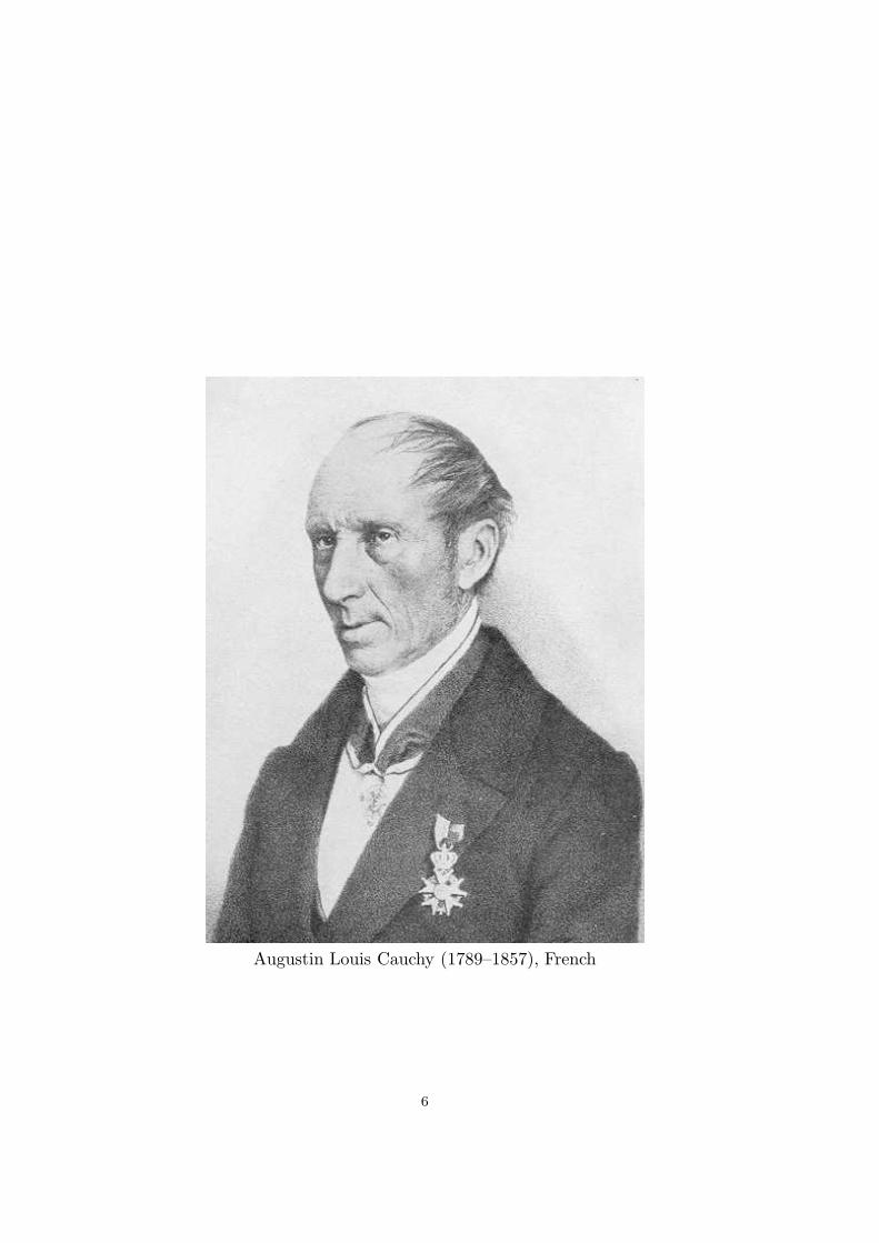
Augustin Louis Cauchy (1789–1857), French

6

i.1

§i. Introduction

i.1. Preliminaries.

In these notes the reader is assumed to have a basic knowledge of thecomplex numbers, here denoted C, including the basic algebraic operationswith complex numbers as well as the geometric representation of complexnumbers in the euclidean plane.

We will therefore without further explanation view a complex numberx+ iy ∈ C as representing a point or a vector (x, y) in R2, and according toour need we shall speak about a complex number or a point in the complexplane. A set of complex numbers can be conceived as a set of points in R2.

Let us recall some basic notions:A complex number z = x+ iy ∈ C has a real part x = Re(z) and an ima-

ginary part y = Im(z), and it has an absolute value (also called its modulus)

r = |z| =√x2 + y2. We recall the important triangle inequality for z, w ∈ C

||z| − |w|| ≤ |z − w| ≤ |z|+ |w|.

For a non-zero complex number z we denote by arg(z) the set of its argu-ments, i.e. the set of real numbers θ such that

z = r(cos θ + i sin θ) .

The pair of numbers (r, θ) for θ ∈ arg(z) are also called polar coordinates forthe complex number z. More about this will be discussed in Section 5.

Every complex number z = x+ iy with x, y ∈ R has a complex conjugatenumber z = x− iy, and we recall that |z|2 = zz = x2 + y2.

As distance between two complex numbers z, w we use d(z, w) = |z − w|,which equals the euclidean distance in R2, when C is interpreted as R2. Withthis distance C is organized as a metric space, but as already remarked,this is the same as the euclidean plane. The concepts of open, closed andbounded subsets of C are therefore exactly the same as for the correspondingsubsets of R2. In this exposition—with a minor exception in Section 9—formal knowledge of the theory of metric spaces is not needed, but we needbasic topological notions from euclidean spaces.

To a ∈ C and r > 0 is attached the open (circular) disc with centre a andradius r > 0, defined as

K(a, r) = z ∈ C | |a− z| < r .

As a practical device we introduce K ′(a, r) as the punctured disc

K ′(a, r) = K(a, r) \ a = z ∈ C | 0 < |a− z| < r .

7

i.2

A mapping f : A→ C defined on a subset A ⊆ C with complex values issimply called a complex function on A. Such a function is called continuousat z0 ∈ A if

∀ε > 0 ∃δ > 0 ∀z ∈ A : |z − z0| < δ ⇒ |f(z)− f(z0)| < ε .

This definition is completely analogous to continuity of functions with realvalues. To a complex function f : A→ C is attached two real functions Re f ,Im f defined on A by

(Re f)(z) = Re(f(z)) , (Im f)(z) = Im(f(z)) , z ∈ A

and connected to f by the equation

f(z) = Re f(z) + i Im f(z) , z ∈ A .

We claim that f is continuous at z0 ∈ A if and only if Re f and Im f areboth continuous at z0.

This elementary result follows from the basic inequalities for the absolutevalue

|Re z| ≤ |z| , | Im z| ≤ |z| , |z| ≤ |Re z| + | Im z| , z ∈ C.

The complex numbers appear when solving equations of second or higherdegree. The point of view that an equation of second degree has no solutionsif the discriminant is negative, was in the 16’th century slowly replaced byan understanding of performing calculations with square roots of negativenumbers. Such numbers appear in the famous work of Cardano called ArsMagna from 1545, and it contains formulas for the solutions to equations ofthe third and fourth degree. Descartes rejected complex roots in his bookLa Geometrie from 1637 and called them imaginary. The mathematicians ofthe 18’th century began to understand the importance of complex numbersin connection with elementary functions like the trigonometric, the exponen-tial function and logarithms, expressed e.g. in the formulas now known asthe formulas of De Moivre and Euler. Around 1800 complex numbers wereintroduced correctly in several publications, and today Caspar Wessel is re-cognized as the one having first published a rigorous geometric interpretationof complex numbers. His work: Om Directionens analytiske Betegning, waspresented at a meeting of The Royal Danish Academy of Sciences and Lettersin 1797 and published two years later. A French translation in 1897 of thework of Wessel made it internationally recognized, and in 1999 appeared anEnglish translation in Matematisk-fysiske Meddelelser 46:1 from the Acad-emy: On the Analytical Representation of Direction, edited by B. Brannerand J. Lutzen. Caspar Wessel was brother of the Danish-Norwegian poetJohan Herman Wessel, who wrote the following about the brother Caspar:

8

i.3

Han tegner Landkaart og læser Loven

Han er saa flittig som jeg er Doven

and in English1

He roughs in maps and studies jurisprudence

He labours hard while I am short of diligence

i.2. Short description of the content.

We shall consider functions f : G→ C defined in an open subset G of C,and we shall study differentiability in complete analogy with differentiabilityof functions f : I → R, defined on an open interval I ⊆ R. Since thecalculation with complex numbers follows the same rules as those for realnumbers, it is natural to examine if the difference quotient

f(z)− f(z0)z − z0

, z, z0 ∈ G , z 6= z0 ,

has a limit for z → z0. If this is the case, we say that f is (complex)differentiable at z0, and for the limit we use the symbol f ′(z0) as in thereal case. It turns out, most surprisingly, that if f is differentiable at allpoints z0 ∈ G, then f is not only continuous as in the real case, but f isautomatically differentiable infinitely often, and is represented by its Taylorseries

f(z) =∞∑

n=0

f (n)(z0)

n!(z − z0)n ,

for all z in the largest open disc K(z0, ρ) around z0 and contained in G.Complex differentiability is a much stronger requirement than real differen-tiability because the difference quotient is required to have one and the samelimit independent of the direction from which z approaches z0. On an inter-val one can only approach a point z0 from left and right, but in the plane wehave infinitely many directions to choose among.

A function, which is complex differentiable at all points of an open set,is called holomorphic in the set. In the literature one also meets the namesanalytic function or differentiable function meaning the same as holomorphicfunction.

The theory of holomorphic functions was completely developed in the19’th century mainly by Cauchy, Riemann and Weierstrass. The theoryconsists of a wealth of beautiful and surprising results, and they are oftenstrikingly different from results about analogous concepts for functions of areal variable.

1I thank Professor Knud Sørensen for this translation

9

i.4

We are also going to study antiderivatives (or primitives) F of a givenfunction f , i.e. functions F such that F ′ = f . It is still “true” that wefind an antiderivative F (z) satisfying F (z0) = 0 by integrating f from z0 toz, but we have a lot of freedom in the complex plane integrating from z0to z. We will integrate along a differentiable curve leading to the conceptof a complex path integral. We then have to examine how this integraldepends on the chosen path from one point to another. The fundamentaldiscovery of Cauchy is roughly speaking that the path integral from z0 to zof a holomorphic function is independent of the path as long as it starts atz0 and ends at z.

It will be too much to introduce all the topics of this treatment. Insteadwe let each section start with a small summary.

Here comes a pertinent warning: In the study of certain properties likecontinuity or integrability of a function with complex values, the reader hasbeen accustomed to a rule stating that such properties are dealt with byconsidering them separately for the real and imaginary part of the function.

It will be a disaster to believe that this rule holds for holomorphic func-tions. The real and imaginary part of a holomorphic function are in factintimately connected by two partial differential equations called the Cauchy-Riemann equations. These equations show that a real-valued function definedon a connected open set is holomorphic if and only if it is constant.

A holomorphic function is extremely rigid: As soon as it is known in atiny portion of the plane it is completely determined.

We have collected a few important notions and results from Analysis inan Appendix for easy reference like A.1,A.2 etc.

Each section ends with exercises. Some of them are easy serving as illu-strations of the theory. Others require some more work and are occasionallyfollowed by a hint.

The literature on complex function theory is enormous. The reader canfind more material in the following classics, which are referred to by the nameof the author:

E. Hille, Analytic function theory I,II. New York 1976-77. (First Edition 1959).

A.I. Markushevich, Theory of functions of a complex variable. Three volumes in one. New

York 1985. (First English Edition 1965-67 in 3 volumes).

W. Rudin, Real and complex analysis. Singapore 1987. (First Edition 1966).

10

1.1

§1. Holomorphic functions

In this section we shall define holomorphic functions in an open subset ofthe complex plane and we shall develop the basic elementary properties ofthese functions. Polynomials are holomorphic in the whole complex plane.

Holomorphy can be characterized by two partial differential equationscalled the Cauchy-Riemann equations.

The sum function of a convergent power series is holomorphic in the discof convergence. This is used to show that the elementary functions sin, cosand exp are holomorphic in the whole complex plane.

1.1. Simple properties.

Definition 1.1. Let G ⊆ C be an open set. A function f : G→ C is called(complex) differentiable at a point z0 ∈ G, if the difference quotient

f(z0 + h)− f(z0)h

has a limit in C for h→ 0. This limit is called the derivative of f at z0, andis denoted f ′(z0). If f is (complex) differentiable at all points of G, then f iscalled holomorphic in G, and the function f ′ : G→ C is called the derivativeof f .

For a function denoted w = f(z) we also write

f ′(z) =dw

dz=df

dz

for the derivative at z ∈ G.The set of holomorphic functions f : G→ C is denoted H(G).

Remark 1.2. For z0 ∈ G there exists r > 0 such that K(z0, r) ⊆ G, andthe difference quotient is then defined at least for h ∈ K ′(0, r).

The assertion that f is differentiable at z0 with derivative f ′(z0) = a, isequivalent to an equation of the form

f(z0 + h) = f(z0) + ha + hε(h) for h ∈ K ′(0, r) , (1)

where r > 0 is such that K(z0, r) ⊆ G, and ε : K ′(0, r) → C is a functionsatisfying

limh→0

ε(h) = 0 .

To see this, note that if f is differentiable at z0 with derivative f ′(z0) = a,then the equation (1) holds with ε(h) defined by

ε(h) =f(z0 + h) − f(z0)

h− a , h ∈ K ′(0, r) .

11

1.2

Conversely, if (1) holds for a function ε satisfying ε(h)→ 0 for h→ 0, then asimple calculation shows that the difference quotient approaches a for h→ 0.

From (1) follows, that if f is differentiable at z0, then f is continuous atz0, because

|f(z0 + h)− f(z0)| = |h| |a+ ε(h)|can be made as small as we wish, if |h| is chosen sufficiently small.

Exactly as for real-valued functions on an interval one can prove that if fand g are differentiable at z0 ∈ G and λ ∈ C, then also λf , f ± g , fg andf/g are differentiable at z0 with the derivatives

(λf)′(z0) = λf ′(z0) ,

(f ± g)′(z0) = f ′(z0)± g′(z0) ,(fg)′(z0) = f(z0)g

′(z0) + f ′(z0)g(z0) ,(f

g

)′(z0) =

g(z0)f′(z0)− f(z0)g′(z0)g(z0)2

, provided that g(z0) 6= 0 .

It is expected that you, the reader, can provide the complete proof of theseelementary facts.

As an example let us show how the last assertion can be proved wheng(z0) 6= 0:

As already remarked, g is in particular continuous at z0, so there existsr > 0 such that g(z0 + h) 6= 0 for |h| < r. For h with this property we get

f(z0 + h)

g(z0 + h)− f(z0)

g(z0)=f(z0 + h)− f(z0)

g(z0 + h)− f(z0)

g(z0 + h)− g(z0)g(z0 + h)g(z0)

.

Dividing by h 6= 0 and letting h→ 0 leads to the assertion.Applying the above to functions assumed differentiable at all points in an

open set, we get:

Theorem 1.3. The set H(G) of holomorphic functions in an open set G ⊆ C

is stable under addition, subtraction, multiplication and division provided thedenominator never vanishes.2

The derivative of a constant function f(z) = k is f ′(z) = 0 and thederivative of f(z) = z is f ′(z) = 1.

More generally, zn is holomorphic in C for n ∈ N0 with the derivative

d

dz(zn) = nzn−1 .

2Using an algebraic language we can say that H(G) is a complex vector space and a

commutative ring.

12

1.3

This can be seen by induction and using the above rule of derivation of aproduct:

d

dz(zn+1) = z

d

dz(zn) +

d

dz(z)zn = z(nzn−1) + zn = (n+ 1)zn.

Using the rule of derivation of a sum, we see that a polynomial

p(z) =n∑

k=0

akzk , ak ∈ C , k = 0, 1, . . . , n ,

is holomorphic in C with the “usual” derivative

p′(z) =n∑

k=1

kakzk−1 .

By the rule of derivation of a fraction it follows that z−n = 1/zn is holo-morphic in C \ 0 for n ∈ N with

d

dz(z−n) = −nz−n−1 .

Also the composition of two functions is differentiated in the usual way:

(f g)′(z0) = f ′(g(z0))g′(z0) . (2)

Here it is assumed that f : G → C is differentiable at g(z0) ∈ G, g : U → C

is assumed differentiable at z0 ∈ U , and we have of course to assume thatg(U) ⊆ G in order to be able to define f g. Note also that U can be anopen interval (g is a differentiable function in the ordinary sense) or an opensubset of C (g is complex differentiable).

To see the above we note that

g(z0 + h) = g(z0) + hg′(z0) + hε(h) ∈ Gf(g(z0) + t) = f(g(z0)) + tf ′(g(z0)) + tδ(t) ,

provided h and t are sufficiently small in absolute value. Furthermore

limh→0

ε(h) = limt→0

δ(t) = 0.

Defining t(h) = hg′(z0) + hε(h), we get for h sufficiently small in absolutevalue:

f(g(z0 + h)) = f(g(z0) + t(h))

= f(g(z0)) + t(h)f ′(g(z0)) + t(h)δ(t(h))

= f(g(z0)) + hf ′(g(z0))g′(z0) + hε(h)

withε(h) = ε(h)f ′(g(z0)) + δ(t(h))(g′(z0) + ε(h)) .

Since limh→0 ε(h) = 0, formula (2) follows.Concerning inverse functions we have:

13

1.4

Theorem 1.4. Suppose that f : G→ C is holomorphic in an open set G ⊆ C

and that f is one-to-one. Then f(G) is open in C and the inverse function3

f−1 : f(G)→ G is holomorphic with

(f−1

)′=

1

f ′ f−1i.e.

(f−1

)′(f(z)) =

1

f ′(z)for z ∈ G .

In particular f ′(z) 6= 0 for all z ∈ G.

Remark 1.5. The theorem is difficult to prove, so we skip the proof here.Look however at exc. 7.15. It is a quite deep topological result that ifonly f : G → C is one-to-one and continuous, then f(G) is open in C andf−1 : f(G)→ G is continuous. See Markushevich, vol. I p. 94.

The formula for the derivative of the inverse function is however easy toobtain, when we know that f−1 is holomorphic: It follows by differentiationof the composition f−1 f(z) = z. Therefore one can immediately derivethe formula for the derivative of the inverse function, and one does not haveto remember it.

If one knows that f ′(z0) 6= 0 and that f−1 is continuous at w0 = f(z0),then it is elementary to see that f−1 is differentiable at w0 with the quoted

derivative.

In fact, if wn = f(zn)→ w0, then we have zn → z0, and

f−1(wn)− f−1(w0)

wn − w0=

zn − z0f(zn)− f(z0)

→ 1

f ′(z0).

1.2. The geometric meaning of differentiability whenf ′(z0) 6= 0f ′(z0) 6= 0f ′(z0) 6= 0.

For real-valued functions of one or two real variables we can draw thegraph in respectively R2 or R3.

For a complex-valued function f defined on a subset G of C the graph(z, f(z)) | z ∈ G is a subset of C2, which can be identified with R4.Since we cannot visualize four dimensions, the graph does not play any role.Instead one tries to understand a holomorphic function f : G→ C, w = f(z),in the following way:

Think of two different copies of the complex plane: The plane of definitionor the z-plane and the image plane or the w-plane. One tries to determine

(i) the image under f of certain curves in G, e.g. horizontal or verticallines;

3We use the notation f−1 for the inverse function to avoid confusion with the reci-

procal f−1 = 1/f .

14

1.5

(ii) the image set f(K) for certain simple subsets K ⊆ G; in particu-lar such K, on which f is one-to-one. In the exercises we shall seeexamples of this.

We shall now analyse image properties of a holomorphic function in theneighbourhood of a point z0, where f

′(z0) 6= 0. In the neighbourhood of apoint z0 where f ′(z0) = 0, the situation is more complicated, and it will notbe analysed here. See however exc. 7.17.

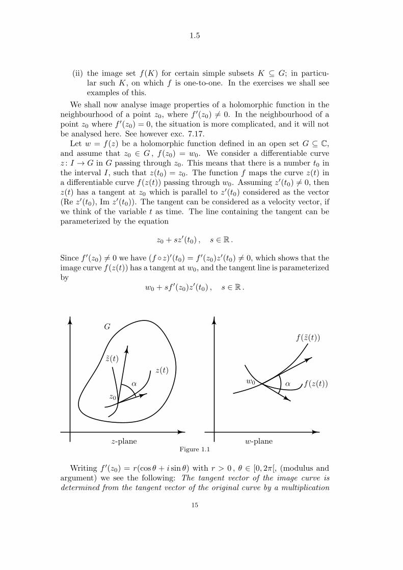
Let w = f(z) be a holomorphic function defined in an open set G ⊆ C,and assume that z0 ∈ G , f(z0) = w0. We consider a differentiable curvez : I → G in G passing through z0. This means that there is a number t0 inthe interval I, such that z(t0) = z0. The function f maps the curve z(t) ina differentiable curve f(z(t)) passing through w0. Assuming z′(t0) 6= 0, thenz(t) has a tangent at z0 which is parallel to z′(t0) considered as the vector(Re z′(t0), Im z′(t0)). The tangent can be considered as a velocity vector, ifwe think of the variable t as time. The line containing the tangent can beparameterized by the equation

z0 + sz′(t0) , s ∈ R .

Since f ′(z0) 6= 0 we have (f z)′(t0) = f ′(z0)z′(t0) 6= 0, which shows that theimage curve f(z(t)) has a tangent at w0, and the tangent line is parameterizedby

w0 + sf ′(z0)z′(t0) , s ∈ R .

G

z0

z-plane

z(t)

z(t)

α w0

w-plane

f(z(t))

f(z(t))

α

Figure 1.1

Writing f ′(z0) = r(cos θ + i sin θ) with r > 0 , θ ∈ [0, 2π[, (modulus andargument) we see the following: The tangent vector of the image curve isdetermined from the tangent vector of the original curve by a multiplication

15

1.6

(dilation, homothetic transformation) with r and a rotation with angle θ.The tangent line of the image curve is determined from the tangent line ofthe original curve by a rotation with angle θ.

We say that f at the point z0 has the dilation constant r = |f ′(z0)| andthe rotation angle θ.

If we consider another curve z(t) passing through z0 and intersecting z(t)under the angle α, meaning that the angle between the tangents at z0 tothe two curves is α, then the image curves f(z(t)) and f(z(t)) also intersecteach other under the angle α, simply because the tangent lines to the imagecurves are obtained from the original tangent lines by a rotation with theangle θ. All the rotations discussed are counterclockwise, corresponding tothe positive orientation of the plane.

We say that f is angle preserving or conformal at the point z0. In par-ticular, two orthogonal curves at z0 (i.e. intersecting each other under theangle π/2) are mapped to orthogonal curves at w0. A function f : G → C,which is one-to-one and conformal at each point of G, is called a conformalmapping. We will later meet concrete examples of conformal mappings.

We see also another important feature. Points z close to and to the left ofz0 relative to the oriented curve z(t) are mapped to points w = f(z) to theleft of the image curve f(z(t)) relative to its orientation.

In fact, the line segment z0 + t(z − z0), t ∈ [0, 1] from z0 to z intersectsthe tangent at z0 under a certain angle v ∈ ]0, π[ and the image curvesf(z0 + t(z − z0)) and f(z(t)) intersect each other under the same angle v.

1.3. The Cauchy-Riemann differential equations.

For a function f : G→ C, where G ⊆ C is open, we often write f = u+ iv,where u = Re f and v = Im f are real-valued functions on G, and theycan be considered as functions of two real variables x, y restricted such thatx+ iy ∈ G, i.e.

f(x+ iy) = u(x, y) + iv(x, y) for x+ iy ∈ G .The following theorem characterizes differentiability of f in terms of proper-ties of u and v.

Theorem 1.6. The function f is complex differentiable at z0 = x0+iy0 ∈ G,if and only if u and v are differentiable at (x0, y0) and the partial derivativesat (x0, y0) satisfy

∂u

∂x(x0, y0) =

∂v

∂y(x0, y0) ;

∂u

∂y(x0, y0) = −

∂v

∂x(x0, y0) .

For a differentiable f we have

f ′(z0) =∂f

∂x(z0) =

1

i

∂f

∂y(z0) .

16

1.7

Proof. Determine r > 0 such that K(z0, r) ⊆ G. For t = h + ik ∈ K ′(0, r)and c = a+ ib there exists a function ε : K ′(0, r)→ C such that

f(z0 + t) = f(z0) + tc+ tε(t) for t ∈ K ′(0, r) , (1)

and we know that f is differentiable at z0 with f ′(z0) = c, if and only ifε(t) → 0 for t → 0. By splitting (1) in its real and imaginary parts and bywriting tε(t) = |t| t|t|ε(t), we see that (1) is equivalent with the following two

real equations

u((x0, y0) + (h, k)) = u(x0, y0) + ha − kb+ |t|σ(h, k) , (2′)

v((x0, y0) + (h, k)) = v(x0, y0) + hb+ ka+ |t|τ(h, k) , (2′′)

where

σ(h, k) = Re( t|t|ε(t)

)and τ(h, k) = Im

( t|t|ε(t)

).

Notice that|ε(t)| =

√σ(h, k)2 + τ(h, k)2 . (3)

By (2′) we see that u is differentiable at (x0, y0) with the partial derivatives

∂u

∂x(x0, y0) = a ,

∂u

∂y(x0, y0) = −b ,

if and only if σ(h, k) → 0 for (h, k) → (0, 0); and by (2′′) we see that v isdifferentiable at (x0, y0) with the partial derivatives

∂v

∂x(x0, y0) = b ,

∂v

∂y(x0, y0) = a ,

if and only if τ(h, k) → 0 for (h, k) → (0, 0). The theorem is now provedsince equation (3) shows that

limt→0

ε(t) = 0⇔ limσ(h, k)(h,k)→(0,0)

= lim τ(h, k)(h,k)→(0,0)

= 0 .

Remark 1.7. A necessary and sufficient condition for f = u+ iv to be holo-morphic in an open set G ⊆ C is therefore that u and v are differentiable, andthat the partial derivatives of u and v satisfy the combined partial differentialequations

∂u

∂x=∂v

∂y,∂u

∂y= −∂v

∂xin G .

17

1.8

These two equations are called the Cauchy-Riemann equations.If we consider f : G → C as a complex-valued function of two real vari-

ables, then differentiability of f at (x0, y0) is exactly that u and v are bothdifferentiable at (x0, y0).

The difference between (complex) differentiability at x0 + iy0 and dif-ferentiability at (x0, y0) is precisely the requirement that the four partialderivatives of u and v with respect to x and y satisfy the Cauchy-Riemannequations.

The Jacobi matrix for the mapping (x, y) 7→ (u, v) is given by

J =

∂u

∂x

∂u

∂y∂v

∂x

∂v

∂y

,

so by using the Cauchy-Riemann equations we find the following expressionfor its determinant called the Jacobian

det J =

(∂u

∂x

)2

+

(∂v

∂x

)2

=

(∂u

∂y

)2

+

(∂v

∂y

)2

= |f ′|2 .

These equations show that the columns of J have the same length |f ′|. Thescalar product of the columns of J is 0 by the Cauchy-Riemann equations,so the columns are orthogonal.

Up to now we have formulated all results about holomorphic functionsfor an arbitrary open set G ⊆ C. We need however a special type of opensubsets of C called domains.

Definition 1.8. An open set G ⊆ C is called a domain, if any two pointsP and Q in G can be connected by a staircase line in G, i.e. it shall bepossible to draw a curve from P to Q inside G and consisting of horizontaland vertical line segments.

Any two different points in an open disc can be connected by a staircaseline consisting of one or two horizontal/vertical line segments, so an opendisc is a domain.

The definition above is preliminary, and we will show later that a domainis the same as a path connected open subset of C, cf. §5.1. In some booksthe word region has the same meaning as domain.

Theorem 1.9. Let G be a domain in C and assume that the holomorphicfunction f : G→ C satisfies f ′(z) = 0 for all z ∈ G. Then f is constant.

Proof. Since

f ′ =∂u

∂x+ i

∂v

∂x=∂v

∂y− i∂u

∂y= 0 ,

18

1.9

we see that the differentiable functions u and v satisfy

∂u

∂x=∂u

∂y=∂v

∂x=∂v

∂y= 0

in G. From ∂u∂x

= 0 we conclude by the mean value theorem that u isconstant on every horizontal line segment in G. In the same way we deducefrom ∂u

∂y= 0 that u is constant on every vertical line segment. Because G is

a domain we see that u is constant in G. The same proof applies to v, andfinally f is constant.

The theorem above does not hold for arbitrary open sets as the followingexample shows.

The function

f(z) =

1 , z ∈ K(0, 1)

2 , z ∈ K(3, 1)

is holomorphic in G = K(0, 1) ∪K(3, 1) with f ′ = 0, but not constant in G.Notice that G is not a domain because 0 and 3 cannot be connected by astaircase line inside G.

The following Corollary is important (but much more is proved in Theorem7.6):

Corollary 1.10. Assume that f : G→ C is holomorphic in a domain G ⊆ C

and that the values of f are real numbers. Then f is a constant function.

Proof. By assumption v = 0 in G, so by the Cauchy-Riemann equations ∂u∂x

and ∂u∂y

are 0 in G. Therefore u and hence f is constant.

1.4. Power series.

The reader is assumed to be acquainted with the basic properties of con-vergence of power series

∑∞0 anz

n, where an ∈ C , z ∈ C.We recall that to any such power series there is associated a number

ρ ∈ [0,∞] called its radius of convergence. For ρ > 0 the series is abso-lutely convergent for any z ∈ K(0, ρ), so we can define the sum functionf : K(0, ρ)→ C of the series by

f(z) =

∞∑

n=0

anzn , |z| < ρ .

If ρ = 0 the power series is convergent only for z = 0 and is of no interest incomplex analysis. The power series is divergent for any z satisfying |z| > ρ.

19

1.10

One way of proving these statements is to introduce the set

T = t ≥ 0 | |an|tn is a bounded sequence ,

and to define ρ = sup T . Clearly [0, ρ[⊆ T . For |z| < ρ choose t ∈ Tsuch that |z| < t < ρ, so by definition there exists a constant M such that|an|tn ≤M, n ≥ 0, hence

|anzn| = |an|tn( |z|t

)n

≤M( |z|t

)n

,

and finally∞∑

n=0

|anzn| ≤M

∞∑

n=0

( |z|t

)n

=M

1− |z|/t <∞.

For |z| > ρ the sequence |an||z|n is unbounded, but then the series∑∞

0 anzn

is divergent.

We will show that the sum function f is holomorphic in the disc of absoluteconvergence K(0, ρ), and we begin with an important Lemma.

Lemma 1.11. A power series and its term by term differentiated powerseries have the same radius of convergence.

Proof. We shall show that ρ = sup T defined above equals ρ′ = sup T ′, where

T ′ = t ≥ 0 | n|an|tn−1 is a bounded sequence .

If for some t > 0 the sequence n|an|tn−1 is bounded, then also |an|tn isbounded, hence T ′ ⊆ T , so we get ρ′ ≤ ρ.

If conversely

|an|tn0 ≤M for n ≥ 0 (1)

for some t0 > 0, we get for 0 ≤ t < t0

n|an|tn−1 = n(t/t0)n−1|an|tn−1

0 ≤ n(t/t0)n−1(M/t0) .

However, since the sequence nrn−1 is bounded when r < 1 (it converges to0), the inequality above shows that also n|an|tn−1 is a bounded sequence.We have now proved that for every t0 ∈ T \ 0 one has [0, t0[⊆ T ′, hencet0 ≤ ρ′ for all such t0, and we therefore have ρ ≤ ρ′.

20

1.11

Theorem 1.12. The sum function f of a power series∑∞

0 anzn is holomor-

phic in the disc of convergence K(0, ρ) (provided ρ > 0), and the derivativeis the sum function of the term by term differentiated power series, i.e.

f ′(z) =∞∑

n=1

nanzn−1 for |z| < ρ .

Proof. We show that f is differentiable at z0, where |z0| < ρ is fixed. Wefirst choose r such that |z0| < r < ρ. For h ∈ C satisfying 0 < |h| < r − |z0|we have

ε(h) :=1

h(f(z0 + h) − f(z0))−

∞∑

n=1

nanzn−10

=

∞∑

n=1

an

(z0 + h)n − zn0

h− nzn−1

0

,

and we have to show that ε(h)→ 0 for h→ 0.For given ε > 0 we choose N such that

∞∑

n=N+1

n|an|rn−1 <ε

4,

which is possible since the series∑∞

1 n|an|rn−1 is convergent. By applying

the identity (xn − yn)/(x− y) =∑nk=1 x

n−kyk−1 we get

(z0 + h)n − zn0h

=n∑

k=1

(z0 + h)n−kzk−10 ,

and since |z0 + h| ≤ |z0|+ |h| < r , |z0| < r we have the estimate

∣∣ (z0 + h)n − zn0h

∣∣ ≤n∑

k=1

rn−krk−1 = nrn−1 .

We now split ε(h) as ε(h) = A(h) +B(h) with

A(h) =

N∑

n=1

an

(z0 + h)n − zn0

h− nzn−1

0

and

B(h) =

∞∑

n=N+1

an

(z0 + h)n − zn0

h− nzn−1

0

21

1.12

and find limh→0

A(h) = 0, since each of the finitely many terms approaches 0.

For |h| sufficiently small (|h| < δ for a suitable δ) we have |A(h)| < ε2 , and

for the tail we have the estimate

|B(h)| ≤∞∑

n=N+1

|an|nrn−1 + |nzn−1

0 |≤ 2

∞∑

n=N+1

|an|nrn−1 <ε

2,

valid for |h| < r − |z0|. For |h| < min(δ, r − |z0|) this leads to |ε(h)| < ε,thereby showing that f is differentiable at z0 with the derivative as claimed.

Corollary 1.13. The sum function f of a power series∑∞

0 anzn is diffe-

rentiable infinitely often in K(0, ρ) and the following formula holds

ak =f (k)(0)

k!, k = 0, 1, . . . .

The power series is its own Taylor series at 0, i.e.

f(z) =∑

n=0

f (n)(0)

n!zn , |z| < ρ .

Proof. By applying Theorem 1.12 k times we find

f (k)(z) =

∞∑

n=k

n(n− 1) · . . . · (n− k + 1)anzn−k , |z| < ρ

and in particular for z = 0

f (k)(0) = k(k − 1) · . . . · 1 ak .

Theorem 1.14. The identity theorem for power series. Assume thatthe power series f(z) =

∑∞0 anz

n and g(z) =∑∞

0 bnzn have radii of con-

vergence ρ1 > 0 and ρ2 > 0. If there exists a number 0 < ρ ≤ min(ρ1, ρ2)such that

f(z) = g(z) for |z| < ρ,

then we have an = bn for all n.

22

1.13

Proof. By the assumptions follow that f (n)(z) = g(n)(z) for all n and all zsatisfying |z| < ρ. By Corollary 1.13 we get

an =f (n)(0)

n!=g(n)(0)

n!= bn.

1.5. The exponential and trigonometric functions.

The reader is assumed to know the power series for the exponential func-tion (as a function of a real variable)

exp(z) =

∞∑

n=0

zn

n!= 1 + z +

z2

2!+ · · · , z ∈ R. (1)

Since this power series converges for all real numbers, its radius of conver-gence is ρ =∞.

We therefore take formula (1) as definition of the exponential function forarbitrary z ∈ C. By Theorem 1.12 we get that exp : C→ C is holomorphic,and since the term by term differentiated series is the series itself, we get

d exp(z)

dz= exp(z) , z ∈ C , (2)

i.e. exp satisfies the differential equation f ′ = f with the initial conditionf(0) = 1.

Another fundamental property of the exponential function is

Theorem 1.15. The exponential function satisfies the functional equation

exp(z1 + z2) = exp(z1) exp(z2) , z1, z2 ∈ C . (3)

Proof. For c ∈ C we consider the holomorphic function

f(z) = exp(z) exp(c− z) , z ∈ C .

If equation (3) is correct, then f(z) has to be a constant function equal toexp(c). This gives us the idea to try to show somehow that f(z) is constant.

Differentiating f we find using (2)

f ′(z) =

(d

dzexp(z)

)exp(c− z) + exp(z)

d

dzexp(c− z)

= exp(z) exp(c− z) − exp(z) exp(c− z) = 0 ,

23

1.14

so by Theorem 1.9 f is a constant, in particular

f(z) = f(0) = exp(0) exp(c) = exp(c).

Setting z = z1, c = z1 + z2 in this formula we obtain

exp(z1 + z2) = exp(z1) exp(z2) .

From the functional equation (3) we deduce that exp(z) 6= 0 for all z ∈ C

since1 = exp(0) = exp(z − z) = exp(z) exp(−z) .

From this equation we further get

exp(−z) = 1

exp(z), z ∈ C . (4)

Defining the number

e := exp(1) =

∞∑

n=0

1

n!(= 2.718 . . . ), (5)

and applying the functional equation n times, yields

exp(nz) = (exp(z))n , n ∈ N,

in particular for z = 1 and z = 1n

exp(n) = en, e = (exp( 1n))n,

showing that

exp( 1n ) =n√e = e

1n .

Raising this to the power p ∈ N gives

(exp(1

n))p = exp(

p

n) = (e

1n )p,

and this expression is usually denoted ep/n. Using (4) we finally arrive at

exp(p

q) = q√ep = e

p

q for p ∈ Z, q ∈ N .

24

1.15

This is the motivation for the use of the symbol ez instead of exp(z), whenz is an arbitrary real or complex number, i.e. we define

ez := exp(z) , z ∈ C , (6)

but we shall remember that the intuitive meaning of ez, i.e. “e multiplied byitself z times”, is without any sense when z /∈ Q.

For a > 0 we define az = exp(z lna) for z ∈ C. Here lna is the naturallogarithm of the positive number a.

It is assumed that the reader knows the power series for the functions sinand cos for real values of z

sin z = z − z3

3!+z5

5!−+ · · · =

∞∑

n=0

(−1)nz2n+1

(2n+ 1)!(7)

cos z = 1− z2

2!+z4

4!−+ · · · =

∞∑

n=0

(−1)nz2n(2n)!

. (8)

These series have the radius of convergence∞, and we use them as definitionof the sine and cosine function for arbitrary z ∈ C.

Notice that cos is an even function, i.e. cos(−z) = cos z, and sin is odd,i.e. sin(−z) = − sin z. Differentiating these power series term by term, wesee that

d

dzsin z = cos z ,

d

dzcos z = − sin z,

and these formulas are exactly as the well-known real variable formulas.

Theorem 1.16. Euler’s formulas (1740s). For arbitrary z ∈ C

exp(iz) = cos z + i sin z

cos z =eiz + e−iz

2, sin z =

eiz − e−iz

2i.

In particular, the following formulas hold

ez = ex(cos y + i sin y) , z = x+ iy , x, y ∈ R

eiθ = cos θ + i sin θ , θ ∈ R,

hence

e2πi = 1 , eiπ = −1 .

25

1.16

Proof. By simply adding the power series of cos z and i sin z we get

cos z + i sin z =

∞∑

n=0

((−1)nz2n(2n)!

+ i(−1)nz2n+1

(2n+ 1)!) =

∞∑

n=0

((iz)2n

(2n)!+

(iz)2n+1

(2n+ 1)!)

= exp(iz) .

Replacing z by −z leads to

exp(−iz) = cos(−z) + i sin(−z) = cos z − i sin z,

which together with the first equation yield the formulas for cos z and sin z.By the functional equation for exp we next get

ez = exp(x) exp(iy) = ex(cos y + i sin y) .

Remark 1.17 By Euler’s formulas we find

u = Re(ez) = ex cos y , v = Im(ez) = ex sin y ,

and we can now directly show that the Cauchy-Riemann equations hold:

∂u

∂x=∂v

∂y= ex cos y ,

∂u

∂y= −∂v

∂x= −ex sin y .

Letting n tend to infinity in

n∑

k=0

zk

k!=

n∑

k=0

(z)k

k!,

we getexp(z) = exp(z) , z ∈ C, (9)

and in particular

| exp(z)|2 = exp(z) exp(z) = exp(z + z) = exp(2Re z),

hence| exp(z)| = exp(Re z) , z ∈ C, (10)

and when z is purely imaginary

| exp(iy)| = 1 , y ∈ R. (11)

26

1.17

(Note that this gives a new proof of the well-known fact cos2 y + sin2 y = 1for y ∈ R.)

We further have:The function f(θ) = eiθ defines a continuous group homomorphism of

the additive group of real numbers (R,+) onto the circle group (T, ·), whereT = z ∈ C | |z| = 1. The equation stating that f is a homomorphism, i.e.

f(θ1 + θ2) = f(θ1)f(θ2) (12)

is a special case of (3) with z1 = iθ1, z2 = iθ2. Taking the real and imaginarypart of this equation, leads to the addition formulas for cosine and sine:

cos(θ1 + θ2) = cos θ1 cos θ2 − sin θ1 sin θ2 (13)

sin(θ1 + θ2) = sin θ1 cos θ2 + cos θ1 sin θ2 . (14)

The formula of De Moivre

(cos θ + i sin θ)n = cosnθ + i sinnθ , θ ∈ R , n ∈ N

is just the equation (exp(iθ))n = exp(inθ) or f(nθ) = f(θ)n, which is aconsequence of (12).

By the functional equation we also get

exp(z + 2πi) = exp(z) exp(2πi) = exp(z) , z ∈ C

which can be expressed like this: The exponential function is periodic withthe purely imaginary period 2πi.

Theorem 1.18. The equation exp(z) = 1 has the solutions z = 2πip, p ∈ Z.The trigonometric functions sin and cos have no other zeros in C than the

ordinary real zeros:

sin z = 0⇔ z = pπ , p ∈ Z .

cos z = 0⇔ z =π

2+ pπ , p ∈ Z .

Proof. Writing z = x+iy, the equation exp(z) = 1 implies | exp(z)| = ex = 1,hence x = 0. This reduces the equation to

exp(iy) = cos y + i sin y = 1

which has the solutions y = 2pπ, p ∈ Z.Assuming sin z = 0, we get by Euler’s formulas that eiz = e−iz . We then

get e2iz = 1, hence 2iz = 2πip, p ∈ Z, which shows that z = pπ, p ∈ Z.

27

1.18

Assuming cos z = 0, we get e2iz = −1 = eiπ , hence ei(2z−π) = 1, whichgives i(2z − π) = 2πip, p ∈ Z, showing that z = π

2+ pπ.

By Theorem 1.18 follows that

tan z =sin z

cos z, cot z =

cos z

sin z

are holomorphic in respectively C \

π2 + πZ

and C \ πZ.

1.6. Hyperbolic functions.

In many situations the functions

sinh z =ez − e−z

2, cosh z =

ez + e−z

2, z ∈ C (1)

play an important role. They are holomorphic in C and are called sinehyperbolic and cosine hyperbolic respectively.

Inserting the power series for ez and e−z , we obtain the following powerseries with infinite radius of convergence

sinh z = z +z3

3!+z5

5!+ · · · =

∞∑

n=0

z2n+1

(2n+ 1)!, (2)

cosh z = 1 +z2

2!+z4

4!+ · · · =

∞∑

n=0

z2n

(2n)!. (3)

Notice that they have the “same form” as the series for sin and cos, butwithout the variation in sign. We observe that sinh is odd and cosh is evenand that the following formulas hold:

d

dzsinh z = cosh z ,

d

dzcosh z = sinh z . (4)

The functions are closely related to the corresponding trigonometric functions

sinh(iz) = i sin z , cosh(iz) = cos z , z ∈ C. (5)

This is a simple consequence of Euler’s formulas or the power series.These formulas are equivalent with

sin(iz) = i sinh z , cos(iz) = cosh z , (6)

28

1.19

and from these we see that

sinh z = 0 ⇐⇒ z = ipπ , p ∈ Z

cosh z = 0 ⇐⇒ z = i(π2+ pπ

), p ∈ Z .

Using Euler’s formulas for cos z and sin z and a small calculation (cf. exc.1.10), we see that the classical formula cos2 z + sin2 z = 1 (assuming z ∈ R)holds for all z ∈ C. Replacing z by iz transforms the equation to

(cosh z)2 + (i sinh z)2 = 1

or equivalentlycosh2 z − sinh2 z = 1 , z ∈ C. (7)

This shows in particular that the points (cosh t, sinh t) for t ∈ R lie on thebranch of the hyperbola

x2 − y2 = 1 , x > 0 .

This is the reason behind the names of the functions.The functions tangent hyperbolic and cotangent hyperbolic are defined by

tanh z =sinh z

cosh z

coth z =cosh z

sinh z,

and they are holomorphic in respectively C \iπ2 + iπZ

and C \ iπZ.

29

1.20

Exercises for §1.

1.1. Prove that f(z) =1

z(1− z) is (complex) differentiable infinitely often

in C \ 0, 1. Find an expression for f (n)(z) for all n ≥ 0.Hint. Write f(z) = 1

z + 11−z .

1.2. Describe the image curves under f(z) = z2 from C to C of the followingplane curves

a) Half-lines starting at 0.b) The circles |z| = r.c) The horizontal line x+ 1

2 i.d) The vertical lines a+ iy, where a > 0 is fixed.

Explain that all image curves from d) intersect the image curve from c)orthogonally, i.e. under right angles.

1.3. Describe the image of horizontal and vertical lines in C under exp z =exeiy , z = x+ iy, and explain that the image curves are orthogonal.

1.4. Consider the functions

f(z) =1

z4 − 1, g(z) =

1

(z2 − 2z + 4− 4i)2.

Explain that f is holomorphic in C \ ± 1,± i and find f ′. Explain that gis holomorphic in C \ −2i, 2 + 2i and find g′.

1.5. Prove that the functions z 7→ Re z and z 7→ z are not differentiable atany point in C.

1.6. Prove that

u(x, y) =x

x2 + y2, v(x, y) = − y

x2 + y2, for (x, y) ∈ R2 \ (0, 0) ,

satisfy the Cauchy-Riemann equations without doing any differentiations.

1.7. Let f : G → C be holomorphic in a domain G and assume that |f | isconstant. Prove that f is constant.

Hint. a) Write f = u + iv and notice that by assumption u2 + v2 isconstant, i.e. u2 + v2 = k ≥ 0 in G. We can also assume that k > 0, becauseif k = 0 then clearly u = v = f = 0.

b) Use ∂∂x(u

2+v2) = ∂∂y (u

2+v2) = 0 and the Cauchy-Riemann-equations

to obtain the linear system of equations

u∂u

∂x− v ∂u

∂y= 0 v

∂u

∂x+ u

∂u

∂y= 0 . (∗)

30

1.21

c) The linear system (∗) with ∂u∂x ,

∂u∂y as unknown has the determinant

u2 + v2. Conclude that ∂u∂x

= ∂u∂y

= 0.

1.8. Prove that if f : C → C is holomorphic and of the form f(x + iy) =u(x)+iv(y), where u and v are real functions, then f(z) = λz+c with λ ∈ R ,c ∈ C.

1.9. Prove the following formulas for n ∈ N, θ ∈ R:

cos(nθ) =

[n/2]∑

k=0

(−1)k(n

2k

)cosn−2k θ sin2k θ

sin(nθ) =

[(n−1)/2]∑

k=0

(−1)k(

n

2k + 1

)cosn−2k−1 θ sin2k+1 θ .

([a] denotes the integer part of a, i.e. [a] is the unique integer p ∈ Z satisfyinga− 1 < p ≤ a.)1.10. Prove the addition formulas

sin(z1 + z2) = sin z1 cos z2 + cos z1 sin z2

cos(z1 + z2) = cos z1 cos z2 − sin z1 sin z2

and the formula(sin z)2 + (cos z)2 = 1

for all z1, z2, z ∈ C.Hint. Euler’s formulas.

1.11. Determine the set of solutions z ∈ C to the equations sin z = 1 andsin z =

√10.

1.12. Assuming x and y ∈ R, prove that

sin(x+ iy) = sinx cosh y + i cosx sinh y .

Use this formula and the Cauchy-Riemann equations to prove that sin isholomorphic with d

dz sin z = cos z.Describe the image of horizontal and vertical lines in C under the sine

function. (Recall that the equationx2

a2− y2

b2= 1 describes a hyperbola, and

the equationx2

a2+y2

b2= 1 describes an ellipse.)

Prove that sine maps the strip

x+ iy | −π

2< x <

π

2, y ∈ R

31

1.22

bijectively onto C \ (]−∞,−1] ∪ [1,∞[).

1.13. Prove that the Cauchy-Riemann equations for f = u + iv can bewritten as one equation:

∂f

∂x+ i

∂f

∂y= 0.

It is customary in advanced complex analysis to introduce the differentialexpressions

∂ =1

2

(∂

∂x− i ∂

∂y

), ∂ =

1

2

(∂

∂x+ i

∂

∂y

).

Prove that ∂f = 0 and f ′(z) = ∂f(z) for a holomorphic function f .

1.14. Prove the following formula for z = x+ iy ∈ C \

π2 + πZ

:

2 tan(x+ iy) =sin(2x)

cos2 x+ sinh2 y+ i

sinh(2y)

cos2 x+ sinh2 y

tan z =1

i

e2iz − 1

e2iz + 1.

1.15. Prove that a power series∑∞

n=0 anzn has radius of convergence ρ =∞

if and only if limn→∞ n√|an| = 0.

1.16. Assume that f, g : G→ C are n times differentiable in the open subsetG of C. Prove Leibniz’ formula for the n’th derivative of a product:

(fg)(n) =n∑

k=0

(n

k

)f (k)g(n−k).

1.17. Prove that the function tan z satisfies tan′ z = 1 + tan2 z, tan′′ z =2 tan z + 2 tan3 z and generally

tan(n) z =n+1∑

k=0

an,k tank z, n = 0, 1, . . . ,

where an,k are non-negative integers.Prove that an,k = 0 when n, k are both even or both odd.Conclude that the Taylor series for tan around 0 has the form

∑∞n=1 tnz

2n−1,where tn = a2n−1,0/(2n− 1)!.

Prove that the Taylor series starts

tan(z) = z +1

3z3 +

2

15z5 + · · · .

32

1.23

(It can be proved that

a2n−1,0 =B2n

2n(22n − 1)22n,

where B2n are the Bernoulli numbers studied in exc. 6.12.)

1.18. Prove that for any z ∈ C

limn→∞

(1 +

z

n

)n= exp(z).

Hint. Prove that for n ≥ 2

exp(z)−(1 +

z

n

)n=

n∑

k=2

zk

k!

1−k−1∏

j=1

(1− j

n)

+∞∑

k=n+1

zk

k!,

and use that the tail ∞∑

k=N+1

|z|kk!

can be made as small as we like, if N is chosen big enough.

1.19. Prove that the radius of convergence ρ for a power series∑∞

0 anzn is

given by Cauchy-Hadamard’s formula

ρ =

(lim supn→∞

n√|an|

)−1

.

(In particular, if limn→∞ n√|an| exists, then ρ is the reciprocal of this limit.)

33

1.24

34

2.1

§2. Contour integrals and primitives

In this section we introduce complex contour integrals. This makes it pos-sible to define the inverse operation of differentiation leading from a functionf to a new one F called the antiderivative or the primitive such that F ′ = f .We first define oriented continuous curves and a path is such a curve whichis piecewise C1.

The estimation lemma 2.8 about contour integrals is very important: It isused repeatedly in these notes.

Theorem 2.13 gives a complete characterization of continuous functionshaving a primitive.

2.1. Integration of functions with complex values.

For a continuous function f : [a, b]→ C we define

∫ b

a

f(t)dt =

∫ b

a

Re f(t)dt+ i

∫ b

a

Im f(t)dt . (1)

Therefore∫ b

af(t)dt is the unique complex number such that

Re

(∫ b

a

f(t)dt

)=

∫ b

a

Re f(t)dt , Im

(∫ b

a

f(t)dt

)=

∫ b

a

Im f(t)dt .

The usual rules of operations with integrals of real-valued functions carryover to complex-valued functions. We have for example

∫ b

a

(f(t) + g(t))dt =

∫ b

a

f(t)dt+

∫ b

a

g(t)dt (2)

∫ b

a

cf(t)dt = c

∫ b

a

f(t)dt , c ∈ C (3)

∫ b

a

f(t)dt = F (b)− F (a) if F ′ = f . (4)

The following estimate, which is exactly as the real version, is somewhattricky to prove.

Theorem 2.1. Let f : [a, b]→ C be a continuous function. Then

∣∣∣∫ b

a

f(t)dt∣∣∣ ≤

∫ b

a

|f(t)|dt .

35

2.2

Proof. The complex number z =∫ b

af(t)dt can be written in the form reiθ,

where r = |z| and θ is an argument for z. By formula (3) we then have

r = ze−iθ =

∫ b

a

e−iθf(t)dt =

∫ b

a

Re(e−iθf(t)

)dt ,

because ∫ b

a

Im(e−iθf(t)

)dt = 0 ,

since the integral of e−iθf(t) is the real number r ≥ 0. We therefore have

∣∣∣∫ b

a

f(t)dt∣∣∣ =

∫ b

a

Re(e−iθf(t)

)dt ≤

∫ b

a

∣∣∣Re(e−iθf(t)

) ∣∣∣dt

≤∫ b

a

∣∣∣e−iθf(t)∣∣∣dt =

∫ b

a

∣∣∣e−iθ∣∣∣ |f(t)|dt =

∫ b

a

|f(t)|dt ,

where we used that Rew ≤ |Rew| ≤ |w| for every w ∈ C and that |e−iθ| = 1.

2.2. Complex contour integrals.

A continuous mapping γ : [a, b] → C is called a continuous curve in C

with parameter interval [a, b], but it is in fact more correct to say that γis a parameterization of an oriented continuous curve in C. If we look atδ : [0, 1] → C defined by δ(t) = γ(a + t(b − a)), then γ and δ are differentparameterizations of the same oriented continuous curve because when tmoves from 0 to 1 then a + t(b − a) moves from a to b and by assumptionδ(t) = γ(a+ t(b− a)).

We say that two continuous mappings γ : [a, b] → C and τ : [c, d] → C

parameterize the same oriented continuous curve, if there exists a continuousand strictly increasing function ϕ of [a, b] onto [c, d] such that τ ϕ = γ. Ifwe consider the variable t as time, different parameterizations just reflect thefact that we can move along the curve with different speed.

The points γ(a) and γ(b) are independent of the parameterization of thecurve and are called the starting point and the end point respectively. Thecurve is called closed if γ(a) = γ(b). The point set γ([a, b]) is also independentof the parameterization and is denoted γ∗. This is intuitively the “set ofpoints on the curve”, where we do not focus on the orientation and the speedof moving along the curve.

36

2.3

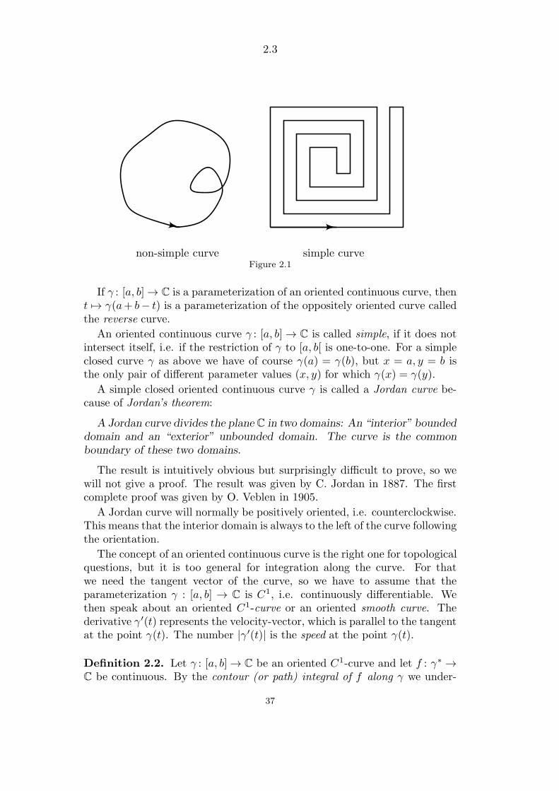
non-simple curve simple curveFigure 2.1

If γ : [a, b]→ C is a parameterization of an oriented continuous curve, thent 7→ γ(a+ b− t) is a parameterization of the oppositely oriented curve calledthe reverse curve.

An oriented continuous curve γ : [a, b]→ C is called simple, if it does notintersect itself, i.e. if the restriction of γ to [a, b[ is one-to-one. For a simpleclosed curve γ as above we have of course γ(a) = γ(b), but x = a, y = b isthe only pair of different parameter values (x, y) for which γ(x) = γ(y).

A simple closed oriented continuous curve γ is called a Jordan curve be-cause of Jordan’s theorem:

A Jordan curve divides the plane C in two domains: An “interior” bounded

domain and an “exterior” unbounded domain. The curve is the common

boundary of these two domains.

The result is intuitively obvious but surprisingly difficult to prove, so wewill not give a proof. The result was given by C. Jordan in 1887. The firstcomplete proof was given by O. Veblen in 1905.

A Jordan curve will normally be positively oriented, i.e. counterclockwise.This means that the interior domain is always to the left of the curve followingthe orientation.

The concept of an oriented continuous curve is the right one for topologicalquestions, but it is too general for integration along the curve. For thatwe need the tangent vector of the curve, so we have to assume that theparameterization γ : [a, b] → C is C1, i.e. continuously differentiable. Wethen speak about an oriented C1-curve or an oriented smooth curve. Thederivative γ′(t) represents the velocity-vector, which is parallel to the tangentat the point γ(t). The number |γ′(t)| is the speed at the point γ(t).

Definition 2.2. Let γ : [a, b]→ C be an oriented C1-curve and let f : γ∗ →C be continuous. By the contour (or path) integral of f along γ we under-

37

2.4

stand the complex number

∫

γ

f =

∫

γ

f(z)dz =

∫ b

a

f(γ(t))γ′(t)dt .

Remark 2.3.(i). The value of

∫γf is not changed if the parameterization γ is replaced by

γ ϕ, where ϕ : [c, d] → [a, b] is a bijective C1-function satisfying ϕ′(t) > 0for all t. This follows from the formula for substitution in an integral.

(ii). Let −γ denote the reverse curve of γ. Then

∫

−γ

f = −∫

γ

f .

(iii). Writing f(z) = u(x, y) + iv(x, y) , where z = x + iy and γ(t) = x(t) +iy(t), we see that

∫

γ

f =

∫ b

a

(u(x(t), y(t)) + iv(x(t), y(t))

)(x′(t) + iy′(t)

)dt

=

∫ b

a

[u(x(t), y(t))x′(t)− v(x(t), y(t))y′(t)]dt

+ i

∫ b

a

[v(x(t), y(t))x′(t) + u(x(t), y(t))y′(t)]dt .

This shows that the real and imaginary part of the path integral are twoordinary tangential curve integrals, and the formula above can be rewritten

=

∫

γ

udx− vdy + i

∫

γ

vdx+ udy =

∫

γ

(u,−v) · ds+ i

∫

γ

(v, u) · ds .

Given two oriented continuous curves γ : [a, b] → C, δ : [c, d] → C suchthat γ(b) = δ(c), we can join the curves such that we first move along γ fromP = γ(a) to Q = γ(b) and then along δ from Q = δ(c) to R = δ(d).

We denote this curve by γ ∪ δ, but in other treatments one can meet thenotation γ + δ. None of these notations matches the ordinary sense of thesymbols ∪ and +.

A parameterization of γ ∪ δ defined on [a, b+ (d− c)] is given by

τ(t) =

γ(t) , t ∈ [a, b]

δ(t+ c− b) , t ∈ [b, b+ (d− c)] .

38

2.5

Assume now that γ, δ above are C1-parameterizations. Then τ is a piecewiseC1-parameterization, because τ | [a, b] is C1 andτ | [b, b+d−c] is C1, but the tangent vectors γ′(b) and δ′(c) can be different.

It is natural to extend Definition 2.2 to the following∫

τ

f =

∫

γ∪δ

f :=

∫

γ

f +

∫

δ

f .

Example 2.4. Let f(z) = z2 and let γ : [0, 1] → C, δ : [1, 2] → C be theC1-curves γ(t) = t2 + it, δ(t) = t + i. Notice that γ passes from 0 to 1 + ialong the parabola y =

√x and δ passes from 1+ i to 2+ i along a horizontal

line, see Figure 2.2.

2+i1+i

1.5

0.75

0.25

0.5

t

2.0

1.0

0.5

1.0

0.0

0.0

Figure 2.2

The composed curve γ ∪ δ is given by the parameterization τ : [0, 2]→ C

defined by

τ(t) =

t2 + it , t ∈ [0, 1]

t+ i , t ∈ [1, 2] ,τ ′(t) =

γ′(t) = 2t+ i , t ∈ [0, 1[

δ′(t) = 1 , t ∈]1, 2] .

Notice that γ′(1) = 2 + i 6= δ′(1) = 1, hence τ ′ is not defined for t = 1. Wefind

∫

τ

f =

∫

γ∪δ

f =

∫ 1

0

(t2 + it)2(2t+ i)dt+

∫ 2

1

(t+ i)2dt

=

∫ 1

0

(2t5 + 5it4 − 4t3 − it2)dt+∫ 2

1

(t2 + 2it− 1)dt

=

[1

3t6 + it5 − t4 − i

3t3]1

0

+

[1

3t3 + it2 − t

]2

1

=

(−2

3+

2

3i

)+

(4

3+ 3i

)=

2

3+

11

3i .

39

2.6

We will now formalize the above as the following extension of Definition2.2.

Definition 2.5. By a path we understand a continuous parameterizationγ : [a, b] → C which is piecewise C1, i.e. there exists a partition a = t0 <t1 < · · · < tn−1 < tn = b such that

γj = γ∣∣∣ [tj−1, tj ] , j = 1, . . . , n

are C1-parameterizations, but there can be kinks at the points γ(tj), becausethe derivative from the right of γj+1 at tj can be different from the derivativefrom the left of γj at tj . A contour is a closed path.

By the integral of f along the path γ we understand the complex number

∫

γ

f =

∫

γ1∪···∪γn

f =

n∑

j=1

∫

γj

f =

n∑

j=1

tj∫

tj−1

f(γ(t))γ′(t)dt . (1)

Remark 2.6. The function f(γ(t))γ′(t), t ∈ [a, b] is piecewise continuous,since it is continuous on each interval ]tj−1, tj[ with limits at the end points.Therefore the function is Riemann integrable in the sense that its real andimaginary parts are Riemann integrable and (1) can be considered as a defi-nition of the integral ∫ b

a

f(γ(t))γ′(t)dt .

Definition 2.7. By the length of a path γ : [a, b] → C, γ(t) = x(t) + iy(t)as in Definition 2.5 we understand the number

L(γ) :=

∫ b

a

|γ′(t)|dt =∫ b

a

√x′(t)2 + y′(t)2dt ,

using that the piecewise continuous function |γ′(t)| is Riemann integrable.

In estimating the size of path integrals the following result is important:

The estimation lemma 2.8. Let γ : [a, b]→ C be a parameterization of apath as above. For a continuous function f : γ∗ → C

∣∣∣∫

γ

f∣∣∣ ≤ max

z∈γ∗

|f(z)|L(γ) , (2)

where L(γ) is the length of the path.

40

2.7

Proof. It is enough to prove the result for a C1-parameterization, since it iseasy to deduce the general result from there. By Theorem 2.1 we have

∣∣∣∫

γ

f∣∣∣ =

∣∣∣∫ b

a

f(γ(t))γ′(t)dt∣∣∣ ≤

∫ b

a

|f(γ(t))| |γ′(t)|dt

≤ maxt∈[a,b]

|f(γ(t))|∫ b

a

|γ′(t)|dt = maxz∈γ∗

|f(z)|L(γ) .

Remark 2.9. In practice it is not necessary to determine

maxz∈γ∗

|f(z)| = maxt∈[a,b]

|f(γ(t))| ,

because very often there is an easy estimate

|f(z)| ≤ K ∀z ∈ γ∗ ,

and hence maxγ∗ |f | ≤ K. By (2) we then get

∣∣∣∫

γ

f∣∣∣ ≤ K L(γ) ,

which in practice is just as useful as (2).

2.3. Primitives.

The concept of primitive or antiderivative as inverse operation of diffe-rentiation is known for functions on an interval. We shall now study theanalogous concept for functions of a complex variable.

Definition 2.10. Let f : G→ C be defined in a domain G ⊆ C. A functionF : G→ C is called a primitive of f if F is holomorphic in G and F ′ = f .

If F is a primitive of f then so is F + k for arbitrary k ∈ C, and in thisway we find all the primitives of f . In fact, if Φ is another primitive of fthen (Φ−F )′ = f − f = 0, and therefore Φ−F is constant by Theorem 1.9.

A polynomial

p(z) = a0 + a1z + · · ·+ anzn , z ∈ C

has primitives in C namely the polynomials

P (z) = k + a0z +a12z2 + · · ·+ an

n+ 1zn+1 ,

41

2.8

where k ∈ C is arbitrary. More generally, the sum of the power series

f(z) =∞∑

n=0

an(z − z0)n , z ∈ K(z0, ρ)

with radius of convergence ρ has the primitives

F (z) = k +

∞∑

n=0

ann+ 1

(z − z0)n+1

in K(z0, ρ). This follows by Lemma 1.11 because F and f have the sameradius of convergence.

Path integrals are easy to calculate if we know a primitive of the integrand.

Theorem 2.11. Suppose that the continuous function f : G → C in thedomain G ⊆ C has a primitive F : G→ C. Then

∫

γ

f(z) dz = F (z2)− F (z1)

for every path γ in G from z1 to z2. In particular∫γf = 0 for every closed

path γ.

Proof. For a path γ : [a, b]→ G such that γ(a) = z1 , γ(b) = z2 we find

∫

γ

f(z) dz =

∫ b

a

f(γ(t))γ′(t) dt

=

∫ b

a

d

dtF (γ(t))dt = F (γ(b))− F (γ(a)) .

For a continuous function f on an interval I we can determine a primitiveby choosing x0 ∈ I and defining

F (x) =

∫ x

x0

f(t)dt , x ∈ I .

Looking for a primitive of f : G→ C, we fix z0 ∈ G and try to define

F (z) =

∫ z

z0

f(t)dt , z ∈ G . (1)

This integral shall be understood as an integral along a path from z0 to z.As a first choice of path one would probably take the straight line from z0 to

42

2.9

z, but then there is a risk of leaving the domain. There are infinitely manypossibilities for drawing paths in G from z0 to z, staircase lines and morecomplicated curves, see Figure 2.3.

z0

zG

Figure 2.3

The question arises if the expression (1) is independent of the path fromz0 to z, because otherwise F (z) is not well-defined by (1).

We shall now see how the above can be realized.

Lemma 2.12. Let f : G→ C be a continuous function in a domain G ⊆ C,and assume

∫γf = 0 for every closed staircase line in G. Then f has a

primitive in G.

Proof. We choose z0 ∈ G. For z ∈ G we define F (z) =∫γzf , where γz

is chosen as a staircase line in G from z0 to z. Such a choice is possiblebecause G is a domain, and we claim that the path integral is independentof the choice of γz. In fact, if δz is another staircase line from z0 to z thenγ := δz ∪ (−γz) is a closed staircase line and hence

0 =

∫

γ

f =

∫

δz

f −∫

γz

f .

In order to prove the differentiability of F at z1 ∈ G with F ′(z1) = f(z1),we fix ε > 0. Since f is continuous at z1 there exists r > 0 such thatK(z1, r) ⊆ G and

|f(z)− f(z1)| ≤ ε for z ∈ K(z1, r) . (2)

To h = h1 + ih2 such that 0 < |h| < r we consider the staircase line ℓ fromz1 to z1 + h, first moving horizontally from z1 to z1 + h1, and then movingvertically from z1 + h1 to z1 + h1 + ih2 = z1 + h. This path belongs toK(z1, r), hence to G. By joining ℓ to γz1 , we have a staircase line γz1 ∪ ℓ

43

2.10

from z0 to z1 + h, and we therefore get

F (z1 + h) − F (z1) =∫

γz1∪ℓ

f −∫

γz1

f =

∫

ℓ

f .

G

z0

z1 + h

z1

K(z1, r)

•

•

Figure 2.4

Since a constant c has the primitive cz, we have by Theorem 2.11

∫

ℓ

c = c(z1 + h)− cz1 = ch .

Putting c = f(z1) we get

1

h(F (z1 + h)− F (z1))− f(z1) =

1

h

∫

ℓ

f − f(z1) =1

h

∫

ℓ

(f(z)− f(z1)) dz ,

hence by the estimation Lemma 2.8, Remark 2.9 and (2)

∣∣∣1

h(F (z1 + h)− F (z1))− f(z1)

∣∣∣ =1

|h|∣∣∣∫

ℓ

(f(z)− f(z1)) dz∣∣∣

≤ 1

|h|εL(ℓ) =|h1|+ |h2||h| ε ≤ 2ε .

Necessary and sufficient conditions for a continuous function to have aprimitive are given next:

Theorem 2.13. For a continuous function f : G→ C on a domain G ⊆ C

the following conditions are equivalent:

(i) f has a primitive.(ii) For arbitrary z1, z2 ∈ G the path integral

∫γf is independent of the

path γ in G from z1 to z2.(iii)

∫γf = 0 for every closed path γ in G.

44

2.11

If the conditions are satisfied, we get a primitive F of f by choosing apoint z0 ∈ G and by defining

F (z) =

∫

γz

f , (3)

where γz is an arbitrary path in G from z0 to z.

Proof. (i) ⇒ (ii) follows from Theorem 2.11.

(ii) ⇒ (iii): Let γ be a closed path in G from z0 to z0 and let δ(t) = z0,t ∈ [0, 1] denote the constant path. By (ii) we have

∫

γ

f =

∫

δ

f =

∫ 1

0

f(δ(t))δ′(t)dt = 0 .

(iii) ⇒ (i): We have in particular∫γf = 0 for every closed staircase line in

G, so by Lemma 2.12 we know that f has a primitive F (z) =∫γzf , where

γz is chosen as a staircase line from a fixed point z0 to z.Finally using that the conditions (i) – (iii) are equivalent, we see that the

expression (3) for F is independent of the choice of path (staircase line ornot) from z0 to z.

Example 2.14. Let Cr denote the circle |z| = r traversed once followingthe positive orientation, i.e. Cr(t) = reit , t ∈ [0, 2π]. For n ∈ Z we find

∫

Cr

dz

zn=

∫ 2π

0

rieit

rneintdt = ir1−n

∫ 2π

0

eit(1−n)dt =

0 , n 6= 1 ,

2πi , n = 1 ,

where we have used that eitk/ik is an ordinary primitive of eitk, when k is anon-zero integer.

For n 6= 1 the result also follows because z−n has the primitive z1−n/(1−n)in C for n ≤ 0, and in C \ 0 for n ≥ 2. Since the value of the integral is6= 0 for n = 1, we conclude that z−1 does not have a primitive in C \ 0.

45

2.12

Exercises for §2.

2.1. Find the value of the path integrals

∫ i

0

dz

(1− z)2 ,∫ 2i

i

cos z dz and

∫ iπ

0

ezdz.

(You are supposed to integrate along the line segment from the lower limitto the upper limit of the integral.)

Find next the value of the three integrals by determining primitives andusing Theorem 2.11.

2.2. Find the value of

∫

γn

dz

z, where γn : [0, 2π]→ C is a parameterization

of the unit circle traversed n times, n ∈ Z \ 0 and given by γn(t) = eitn.

2.3. Prove that ∫

γ

z

(z2 + 1)2dz = 0 ,

if γ is a closed path in C \ ±i.

2.4. Prove that ∫

γ

P (z)dz = 0

for every polynomial P and every closed path γ in C.

2.5. Prove that A(γ) = 12i

∫γz dz is a real number for every closed path γ in

C.Hint. Writing γ(t) = x(t) + iy(t), t ∈ [a, b], prove that

A(γ) =1

2

∫ b

a

∣∣∣∣x(t) y(t)x′(t) y′(t)

∣∣∣∣ dt .

Determine A(γn) for γn(t) = eint, t ∈ [0, 2π], n = ± 1. For a simple closedpath γ, explain that A(γ) can be interpreted as the area bounded by γcounted positively or negatively in accordance with the orientation of γ.

2.6. Assume that f and g are holomorphic functions in a domain G andassume for convenience also that f ′ and g′ are continuous (these assumptionswill later be shown to be superfluous, see Theorem 4.8). Prove for any closedpath γ in G: ∫

γ

f ′(z)g(z)dz = −∫

γ

f(z)g′(z)dz .

46

3.1

§3. The theorems of Cauchy

The main result of this section is Cauchy’s integral theorem: The integralof a holomorphic function along a closed path is zero provided the domainof definition is without holes.

From this result we deduce Cauchy’s integral formula, expressing the valueof a holomorphic function at an interior point of a disc in terms of the valueson the circumference. The result is very surprising: Knowing just a tiny bitof a holomorphic function is enough to determine it in a much bigger set.

These two results are fundamental for the rest of the notes.

3.1. Cauchy’s integral theorem.

We know that f : G→ C has a primitive provided the integral of f alongevery closed path is zero. We also know that continuity of f : G → C isnot enough (unlike real analysis) to secure the existence of a primitive. Evensuch a nice and elementary function as f(z) = 1/z defined on G = C \ 0does not have a primitive according to Example 2.14.

It turns out that for f : G → C to have a primitive, we have to imposeconditions on f as well as on the domainG. This is the fundamental discoveryof Cauchy around 1825.

The requirement for G is roughly speaking that it does not contain holes.The domain C \ 0 has a hole at 0. We will now make this intuitive wayof speaking precise.

A domainG ⊆ C is called simply connected if for any two continuous curvesγ0, γ1 in G having the same starting point a and the same end point b, it ispossible to deform γ0 continuously into γ1 within G. Assuming that the twocurves have [0, 1] as common parameter interval, a continuous deformationmeans precisely that there exists a continuous function H : [0, 1]× [0, 1]→ G,such that

H(0, t) = γ0(t) , H(1, t) = γ1(t) for t ∈ [0, 1] ,

and

H(s, 0) = a , H(s, 1) = b for s ∈ [0, 1].

For every s ∈ [0, 1] the parameterization t 7→ H(s, t) determines a contin-uous curve γs from a to b, and when s varies from 0 to 1 this curve variesfrom γ0 to γ1. The function H is called a homotopy.

Intuitively, a simply connected domain is a domain without holes.A subset G of C is called star-shaped if there exists a point a ∈ G such

that for each z ∈ G the line segment from a to z is contained in G. In acolourful way we can say that a light source at a is visible from each point zof G. We also say that G is star-shaped with respect to such a point a.

47

3.2

We mention without proof that a star-shaped domain is simply connected,cf. exc. 3.4.

A subset G of C is called convex if for all a, b ∈ G the line segment betweena and b belongs to G, i.e. if

γ(t) = (1− t)a+ tb ∈ G for t ∈ [0, 1] .

A convex set is clearly star-shaped with respect to any of its points. Thereforea convex domain is simply connected.

Removing a half-line from C leaves a domain which is star-shaped withrespect to any point on the opposite half-line, see Example A of Figure 3.1.

An angular domain, i.e. the domain between two half-lines starting atthe same point, is star-shaped. It is even convex if the angle is at most 180degrees, but not convex if the angle is more than 180 degrees as in ExampleB (the grey part). The domain outside a parabola (Example C) is simplyconnected but not star-shaped. Removing one point from a domain (ExampleD) or removing one or more closed discs (Example E) leaves a domain whichis not simply connected.

A B C

D E

Figure 3.1

48

3.3

Theorem 3.1 (Cauchy’s integral theorem). Let f : G → C be a holo-morphic function in a simply connected domain G ⊆ C and let γ be a closedpath in G. Then ∫

γ

f(z)dz = 0 .

Cauchy gave the result in 1825. Cauchy worked with continuously differen-tiable functions f , i.e. f is assumed to be holomorphic and f ′ to be contin-uous.

For a differentiable function f : I → R on an interval it can happen thatf ′ has discontinuities. Here is an example with I = R and

f(x) =

x2 sin 1

x , x 6= 0

0 , x = 0f ′(x) =

2x sin 1

x − cos 1x , x 6= 0

0 , x = 0 .

For a complex differentiable (holomorphic) function f : G → C defined onan open set, it turns out most surprisingly that f ′ is continuous. This wasdiscovered by the French mathematician E. Goursat in 1899. He gave aproof of Cauchy’s integral theorem without assuming f ′ to be continuous.The main point in the proof is Goursat’s Lemma below, but the proof thatf ′ is continuous will first be given in Theorem 4.8.

Lemma 3.2 (Goursat’s Lemma). Let G ⊆ C be open and let f ∈ H(G).Then ∫

∂f(z) dz = 0

for every solid triangle ⊆ G (meaning that all points bounded by the sidesare contained in G).

Proof. The contour integral along the boundary ∂ of a triangle shall beunderstood in the following sense: We move along the sides of the trianglefollowing the positive orientation. Once we have proved that this integral iszero, the path integral using the negative orientation will of course also bezero.

We draw the segments between the midpoints of the sides of the triangle,see Figure 3.2.4 Now is divided in four triangles(1), . . . ,(4) as shown onthe figure, and we use the indicated orientations of the sides of the triangles.Using e.g. that the pair of triangles ((1),(4)), ((3),(4)), ((4),(2))have a common side with opposite orientations, we get

I =

∫

∂f =

4∑

i=1

∫

∂(i)

f .

4It is only for simplicity of drawing that the triangle is isosceles.

49

3.4

We claim that at least one of the four numbers∫∂(i) f must have an abso-

lute value ≥ 14 |I|, because otherwise we would get |I| < |I| by the triangle

inequality. Let one of the triangles with this property be denoted 1, hence

|I| ≤ 4∣∣∫

∂1

f∣∣ .

−→−→ −→ւ∆(1)տ

←−ց∆(4) ր ւ∆(2)տ

−→ւ ∆(3) տ

ւ∆ տ

Figure 3.2

We now apply the same procedure to1. Therefore, there exists a triangle2, which is one of the four triangles in which 1 is divided, such that

|I| ≤ 4∣∣∫

∂1

f∣∣ ≤ 42

∣∣∫

∂2

f∣∣ .

Continuing in this way we get a decreasing sequence of closed triangles ⊃1 ⊃ 2 ⊃ . . . such that

|I| ≤ 4n∣∣∫

∂n

f∣∣ for n = 1, 2, . . . . (1)

We now have ∞⋂

n=1

n = z0

for a uniquely determined point z0 ∈ C.In fact, choosing zn ∈ n for each n, the sequence (zn) has a convergent

subsequence with limit point z0 by the Bolzano-Weierstrass theorem. It iseasy to see that z0 ∈ ∩∞1 n, and since the sidelength of the triangles isdivided by two in each step, there is only one number in the intersection.If L denotes the length of ∂, then the length of ∂n equals 2−nL. We nowuse that f is differentiable at z0. If ε > 0 is fixed we can find r > 0 such that

|f(z)− f(z0)− f ′(z0)(z − z0)| ≤ ε|z − z0| for z ∈ K(z0, r) ⊆ G . (2)

50

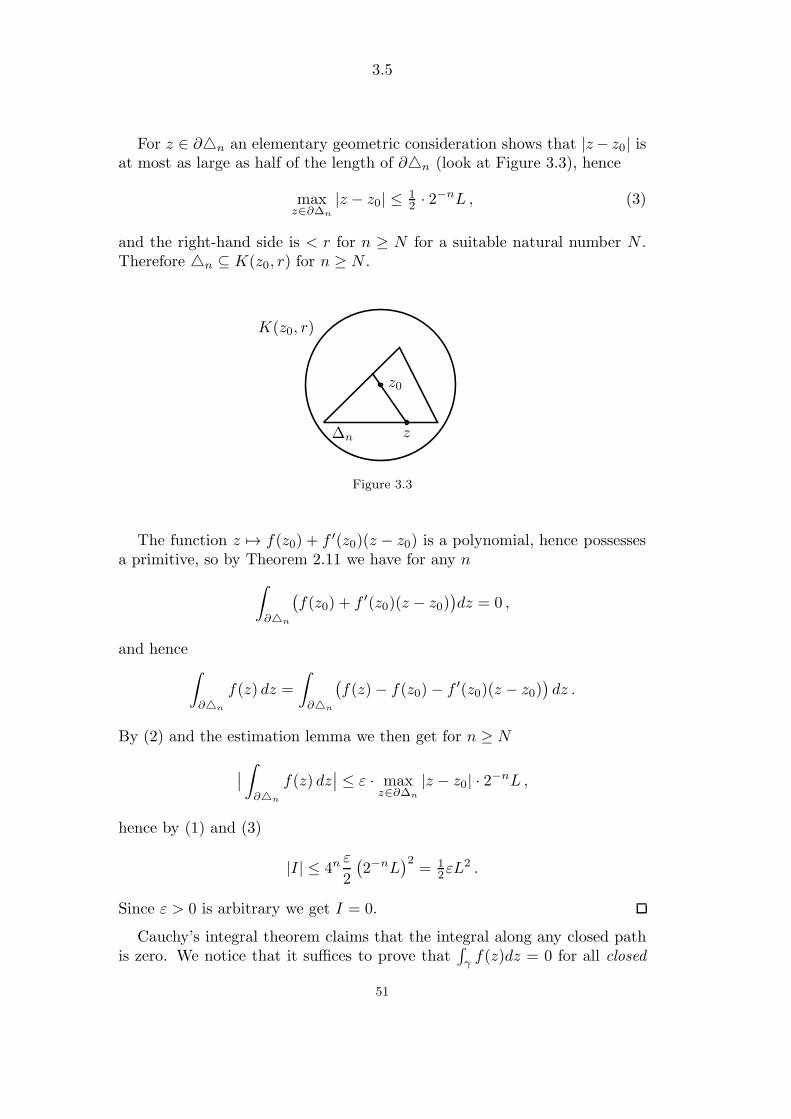
3.5

For z ∈ ∂n an elementary geometric consideration shows that |z− z0| isat most as large as half of the length of ∂n (look at Figure 3.3), hence

maxz∈∂∆n

|z − z0| ≤ 12 · 2−nL , (3)

and the right-hand side is < r for n ≥ N for a suitable natural number N .Therefore n ⊆ K(z0, r) for n ≥ N .

∆n z

z0

K(z0, r)

Figure 3.3

The function z 7→ f(z0) + f ′(z0)(z − z0) is a polynomial, hence possessesa primitive, so by Theorem 2.11 we have for any n

∫

∂n

(f(z0) + f ′(z0)(z − z0)

)dz = 0 ,

and hence∫

∂n

f(z) dz =

∫

∂n

(f(z)− f(z0)− f ′(z0)(z − z0)

)dz .

By (2) and the estimation lemma we then get for n ≥ N

∣∣∫

∂n

f(z) dz∣∣ ≤ ε · max

z∈∂∆n

|z − z0| · 2−nL ,

hence by (1) and (3)

|I| ≤ 4nε

2

(2−nL

)2= 1

2εL2 .

Since ε > 0 is arbitrary we get I = 0.

Cauchy’s integral theorem claims that the integral along any closed pathis zero. We notice that it suffices to prove that

∫γf(z)dz = 0 for all closed

51

3.6

staircase lines in G, because then f has a primitive in G by Lemma 2.12,and Theorem 2.11 next shows that

∫γf(z)dz = 0 for arbitrary closed paths.

Goursat’s Lemma tells us that∫∂ f(z)dz = 0 for all solid triangles in G.

Given an arbitrary closed staircase line in G, it is now quite obvious to tryto draw extra line segments in order to split the staircase line in trianglesand then use Goursat’s Lemma for each of these triangles.

The problem is then to secure that all these extra line segments remainwithin G, and it is here we need the assumption that the domain is simplyconnected.

For an arbitrary simply connected domain this becomes quite technical,and we skip this proof.

We will give the complete proof for a star-shaped domain and this willsuffice for all our applications in this course.

Theorem 3.3 (Cauchy’s integral theorem for a star-shaped do-main). Let G be a star-shaped domain and assume that f ∈ H(G). Then

∫

γ

f(z)dz = 0

for every closed path γ in G.

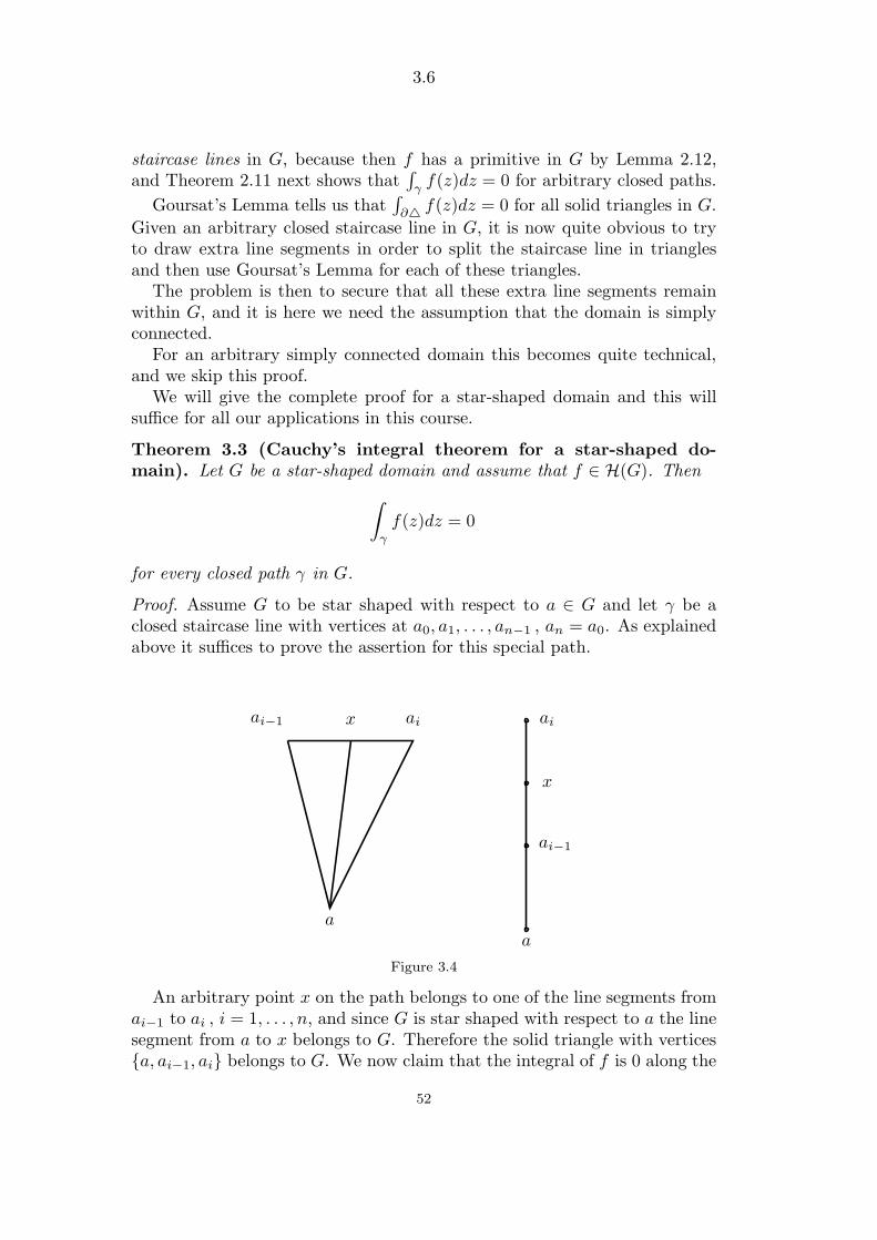
Proof. Assume G to be star shaped with respect to a ∈ G and let γ be aclosed staircase line with vertices at a0, a1, . . . , an−1 , an = a0. As explainedabove it suffices to prove the assertion for this special path.

a

ai−1 x ai ai

x

ai−1

a

Figure 3.4

An arbitrary point x on the path belongs to one of the line segments fromai−1 to ai , i = 1, . . . , n, and since G is star shaped with respect to a the linesegment from a to x belongs to G. Therefore the solid triangle with verticesa, ai−1, ai belongs to G. We now claim that the integral of f is 0 along the

52

3.7

path consisting of the following 3 segments: From a to ai−1, from ai−1 to aiand from ai to a. In fact, either the 3 points form a non-degenerate triangleand the result follows from Goursat’s lemma, or the 3 points lie on a line,and in this case the claim is elementary.

Summing these n vanishing integrals yields

n∑

i=1

∫

∂a,ai−1,aif = 0 .

Each line segment from a to ai , i = 1, . . . , n, gives two contributions withopposite sign, so they cancel each other and what remains is

∫γf , which

consequently is 0.

Remark 3.4. Even ifG is not simply connected, it may happen that∫γf = 0

for certain f ∈ H(G) and certain closed paths γ in G, e.g. in the followingcases

(a): f has a primitive in G(b): γ is a path in a simply connected sub-domain G1 of G.Notice that ∫

∂K(a,r)

dz

z= 0 for a 6= 0 , 0 < r < |a|.

Important notation Here and in the following we always use the shortnotation ∂K(a, r) to indicate the path which traverses the circle counter-clockwise. The function 1/z is holomorphic in G = C \ 0, which is a nonsimply connected domain, but the path is contained in a half-plane G1 (makea drawing), and therefore the integral is 0.

Combining the Cauchy integral theorem (Theorem 3.1) and Theorem 2.13we get:

Theorem 3.5. Every holomorphic function in a simply connected domainhas a primitive there.

3.2. Cauchy’s integral formula.

Let G be a domain, let z0 ∈ G and assume that f ∈ H(G\z0). Supposethat we want to calculate the integral of f along a simple closed path C,traversed counterclockwise around the point z0.

As an application of Cauchy’s integral theorem we shall see that it will bepossible in many cases to replace C by another simple closed path K in G,likewise traversed counterclockwise around z0, i.e.

∫

C

f(z) dz =

∫

K

f(z) dz . (1)

53

3.8

The idea to prove such a result is to insert a number of cuts (line segments)from C to K (four at the figure), thereby creating a finite number of “small”closed paths γi, each of them consisting of 1) a part of C, 2) a cut, 3) a partof K with the opposite orientation, 4) a cut. We assume that it is possible tomake the cuts in such a way that each γi is a closed path within a star-shapedsub-domain of G \ z0, thereby proving that

∫γif = 0. Since each cut will

contribute with two integrals of opposite sign, we finally get

0 =∑∫

γi

f =

∫

C

f +

∫

−K

f ,

z0.

K

C

z0.γ1

γ2γ3

γ4

Figure 3.5

which shows the claim ∫

C

f =

∫

K

f .

Before giving a concrete example of this principle, we need:

Lemma 3.6. Let G ⊆ C be open and assume that K(a, r) ⊆ G. Then thereexists R > r such that K(a, R) ⊆ G. (“There is always room for a largerdisc”).

Proof. If G = C every R > r can be used. Assume next that G 6= C, hence∁G 6= ∅, and define

R = inf|z − a| | z ∈ ∁G .

Then K(a, R) ⊆ G, and since K(a, r) ⊆ G by assumption we have r ≤ R.We have to exclude the possibility r = R.

By Lemma A.1 in the Appendix with K = a, F = ∁G there exists

y′ ∈ ∁G such that |a − y′| = R. Assuming r = R we get y′ ∈ K(a, r), hencey′ ∈ G, but this is a contradiction.

54

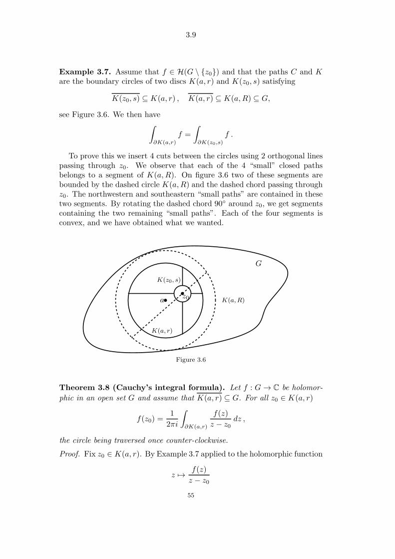
3.9

Example 3.7. Assume that f ∈ H(G \ z0) and that the paths C and Kare the boundary circles of two discs K(a, r) and K(z0, s) satisfying

K(z0, s) ⊆ K(a, r) , K(a, r) ⊆ K(a, R) ⊆ G,

see Figure 3.6. We then have∫

∂K(a,r)

f =

∫

∂K(z0,s)

f .

To prove this we insert 4 cuts between the circles using 2 orthogonal linespassing through z0. We observe that each of the 4 “small” closed pathsbelongs to a segment of K(a, R). On figure 3.6 two of these segments arebounded by the dashed circle K(a, R) and the dashed chord passing throughz0. The northwestern and southeastern “small paths” are contained in thesetwo segments. By rotating the dashed chord 90 around z0, we get segmentscontaining the two remaining “small paths”. Each of the four segments isconvex, and we have obtained what we wanted.

•a•z0

G

K(a,R)

K(z0, s)

K(a, r)

Figure 3.6

Theorem 3.8 (Cauchy’s integral formula). Let f : G→ C be holomor-

phic in an open set G and assume that K(a, r) ⊆ G. For all z0 ∈ K(a, r)

f(z0) =1

2πi

∫

∂K(a,r)

f(z)

z − z0dz ,

the circle being traversed once counter-clockwise.

Proof. Fix z0 ∈ K(a, r). By Example 3.7 applied to the holomorphic function

z 7→ f(z)

z − z055

3.10

in G \ z0, we see that∫

∂K(a,r)

f(z)

z − z0dz =

∫

∂K(z0,s)

f(z)

z − z0dz

for 0 < s < r − |a − z0|. Inserting the parameterization θ 7→ z0 + seiθ ,θ ∈ [0, 2π], of ∂K(z0, s) we find

∫

∂K(z0,s)

dz

z − z0=

∫ 2π

0

sieiθ

seiθdθ = 2πi ,

hence

I =

∫

∂K(a,r)

f(z)

z − z0dz − 2πi f(z0) =

∫

∂K(z0,s)

f(z)− f(z0)z − z0

dz .

By the estimation lemma we then get

|I| ≤ sup∣∣f(z)− f(z0)

z − z0∣∣ | |z − z0| = s · 2πs

= 2π sup∣∣f(z)− f(z0)

∣∣ | |z − z0| = s ,

but since f is continuous at z0, the given supremum approaches 0 for s→ 0,and we conclude that I = 0.

Corollary 3.9. Let f : G→ C be holomorphic in an open set G and assumethat K(a, r) ⊆ G. Then

f(a) =1

2π

∫ 2π

0

f(a+ reiθ) dθ .

Proof. We apply the theorem for z0 = a and insert the parameterization

θ 7→ a+ reiθ , θ ∈ [0, 2π] .

Cauchy’s integral formula shows that knowledge of the values of a holo-morphic function on a circle ∂K(a, r) determines the values of the functionin the disc. The Corollary tells us that the value at the centre of the circleis the mean value along the boundary.

Example 3.10. Cauchy’s integral formula can be used to find the value ofcertain contour integrals:

∫

∂K(0,2)

sin z

1 + z2dz =

1

2i

∫

∂K(0,2)

sin z

z − i dz −1

2i

∫

∂K(0,2)

sin z

z + idz

= π sin(i)− π sin(−i) = 2π sin(i) = πi(e− 1

e) .

56

3.11

Example 3.11. Using Cauchy’s integral theorem, we will prove the formula

1√2π

∫ ∞

−∞e−

12 t

2

eitbdt = e−12 b

2

, b ∈ R ,

expressing that e−12 t

2

equals its Fourier transform up to a constant factor.For b = 0 the formula reads

1√2π

∫ ∞

−∞e−

12 t

2

dt = 1.

This we will not prove but consider as a well-known fact from probabilitytheory about the normal or Gaussian density. Using that cos is an evenfunction and that sin is odd, we find from Euler’s formulas

∫ ∞

−∞e−

12 t

2

eitbdt =

∫ ∞

−∞e−

12 t

2

cos(tb) dt ,

showing that it is enough to prove the formula for b > 0.Fixing b > 0, we integrate f(z) = exp(−1

2z2) along the boundary of the

rectangle of Figure 3.7. This integral is 0 by the Cauchy integral theorembecause f is holomorphic in C.

Parameterizations of the four sides of the rectangle are given as

γ1(t) = t , t ∈ [−a, a] ,γ2(t) = a+ it , t ∈ [0, b] ,

γ3(t) = −t+ ib , t ∈ [−a, a] ,γ4(t) = −a + i(b− t) , t ∈ [0, b] ;

(−a, b)

γ4

(−a, 0)

γ3 (a, b)

γ2

(a, 0)γ1

Figure 3.7

and we get

∫

γ1

f =

∫ a

−a

e−12 t

2

dt ,

∫

γ3

f = −e 12 b

2

∫ a

−a

e−12 t

2

eitbdt ,

∫

γ2

f = ie−12a

2

∫ b

0

e12 t

2

e−iatdt ,

∫

γ4

f = −ie− 12a

2

∫ b

0

e12 (b−t)2eia(b−t)dt ,

57

3.12

hence ∣∣∫

γ2

f∣∣ ,∣∣∫

γ4

f∣∣ ≤ e− 1

2a2

b e12 b

2 → 0 for a→∞ .

Moreover,

lima→∞

∫

γ3

f = −e 12 b

2

∫ ∞

−∞e−

12 t

2

eitbdt ,

and

lima→∞

∫

γ1

f =

∫ ∞

−∞e−

12 t

2

dt =√2π ,

so letting a→∞ in∑4

i=1

∫γif = 0, we get

√2π + 0− e 1

2 b2

∫ ∞

−∞e−

12 t

2

eitbdt+ 0 = 0 ,

showing the formula.

58

3.13

Exercises for §3.

3.1. Determine the value of

∫

∂K(0,1)

dz

(z − a)(z − b) ,

when (i) |a| , |b| < 1 , (ii) |a| < 1 , |b| > 1 , (iii) |a| , |b| > 1.

3.2. Calculate the contour integrals

∫

∂K(0,2)

ez

z − 1dz,

∫

∂K(0,2)

ez

πi− 2zdz .

3.3. Prove that a convex domain G ⊆ C is simply connected.

3.4. Prove that a star-shaped domain G ⊆ C is simply connected.Hint. Reduce the assertion to a domain G which is star-shaped with

respect to 0.For such a domain G let γ0 be a continuous curve in G from a ∈ G to b ∈ G

with parameter interval [0, 1]. Prove that the expression H(s, t) defined by

H(s, t) =

(1− 2t)a , for t ∈ [0, 12s] ,

(1− s)γ0(

t− 12 s

1−s

), for t ∈ [ 1

2s, 1− 1

2s[ ,

(2t− 1)b , for t ∈ [1− 12s, 1] ,

is a homotopy, deforming γ0 continuously to the curve

γ1(t) =

(1− 2t)a , for t ∈ [0, 12 ] ,

(2t− 1)b , for t ∈ [1− 12, 1] ;

and use this to finish the proof.

3.5. Let G be a domain which is star-shaped with respect to z0 ∈ G. Forevery z ∈ G let [z0, z] denote the line segment from z0 to z with the param-eterization γ(t) = (1− t)z0 + tz.

Prove directly from Goursat’s lemma that if f ∈ H(G) then F : G → C

defined by

F (z) =

∫

[z0,z]

f

is a primitive of f satisfying F (z0) = 0.

59

3.14

3.6. The domain G = C\]−∞, 0] is star-shaped with respect to 1. By exc.3.5 the formula

L(z) =

∫

[1,z]

dt

t, z ∈ G

defines a primitive of 1/z in G.Writing z = reiθ, θ ∈]− π, π[, r > 0, show that

L(reiθ) = log r + iθ .

Hint. Use the path from 1 to r followed by the arc of circle from r til reiθ.(We prove in section 5 that L(z) = Log z, the principal logarithm of z.)

3.7. Let G be an open disc, let a ∈ G and let b, c be different points on theboundary of the disc. Let U be the domain bounded by the line segments[a, b], [a, c] and one of the two arcs between b and c. Show that U is convexif the angle at a is ≤ π. Show that U is star-shaped but not convex if theangle at a is > π. (U is a piece of tart).

Use such a domain U to show that 2 “small paths” are sufficient in Ex-ample 3.7.

3.8. Consider the domain

G = C \ iy | y ∈ R, |y| ≥ 1

and prove that it is star-shaped with respect to 0. Define the functionArctan : G→ C by

Arctan z =

∫

[0,z]

dw

1 + w2=

∫ 1

0

zdt

1 + t2z2, z ∈ G.

In accordance with exc. 3.5 Arctan is holomorphic on G with the derivative

d

dzArctan z =

1

1 + z2.

Prove that Arctan |R is the inverse function of tan :]−π

2 ,π2

[→ R.

(One can show that Arctan maps G bijectively onto the strip

z = x+ iy | −π

2< x <

π

2

,

and is the inverse function of tan restricted to that strip.)Prove that

Arctan z = z − z3

3+z5

5−+ · · · for |z| < 1 .

60

3.15

3.9. (Fresnel’s integrals). Calculate the integrals

∫ ∞

0

sin(x2)dx =

∫ ∞

0

cos(x2)dx =

√π

2√2,

which are to be understood as limr→∞

∫ r

0.

Hint. a) Use that∫γr

exp(iz2)dz = 0, where γr for r > 0 denotes the path

along the boundary of the sector enclosed by the x-axis, the line y = x andthe arc reit, t ∈

[0, π4

].

b) Let r →∞ and use (example 3.11),

limr→∞

∫ r

0

e−x2

dx =1

2

√π

as well as sin 2t ≥ t for t ∈[0, π4

](cf. c)) in order to prove the result.

c) Show that min sin 2tt | t ∈

]0, π4

] = 4

π > 1.

3.10. Consider the set G = C \ Z.1) Show that G is a domain, i.e. that G is open and that any two points

of G can be joined by a staircase line.2) Is G convex?, star-shaped?, simply connected?3) Show that

f(z) = 1/ sin(πz), z ∈ Gis holomorphic in G.

4) Define γT (t) =12+ it, δT (t) =

32+ it, t ∈ [−T, T ].

Show that

limT→∞

∫

γT

f(z) dz = i

∫ ∞

−∞

dt

cosh(πt), lim

T→∞

∫

δT

f(z) dz = −i∫ ∞

−∞

dt

cosh(πt)

5) Define γT,a(t) = a+ it, t ∈ [−T, T ], where a ∈ R \ Z. Show that

ϕ(a) := limT→∞

∫

γT,a

f(z) dz

is constant in each of the intervals ]n, n+1[, n ∈ Z. (Notice that ϕ(a) changessign when a jumps from ]0, 1[ to ]1, 2[.)

Hint. For n < a < b < n + 1 use the Cauchy integral theorem for therectangle with corners a± iT, b± iT and let T →∞.

61

3.16

Bernhard Riemann (1826–1866), German

62

4.1

§4. Applications of Cauchy’s integralformula

In section 4.2 we shall apply the Cauchy integral formula to prove that aholomorphic function is differentiable infinitely often and is equal to the sumof its Taylor series. In the proof we need the concept of uniform convergence,which is treated in section 4.1. The set of holomorphic functions is stablewith respect to local uniform convergence. This clearly makes it an importantconcept, which will be developed in section 4.4.

Liouville’s theorem and the fundamental theorem of algebra appear unex-pectedly.

4.1. Sequences of functions.

LetM be an arbitrary non-empty set. In the applicationsM will typicallybe a subset of C.

A sequence of functions fn : M → C is said to converge pointwise to thefunction f :M → C if for all x ∈M

limn→∞

fn(x) = f(x) .

Using quantifiers this can be expressed:

∀x ∈M ∀ε > 0 ∃N ∈ N ∀n ∈ N (n ≥ N ⇒ |f(x)− fn(x)| ≤ ε) . (1)

Examples: 1) Let M = R and fn(x) = | sinx|n, n = 1, 2, . . . . Then

limn→∞

fn(x) =

1 for x = π

2+ pπ , p ∈ Z

0 for x ∈ R \

π2 + Zπ

,

i.e. fn : R → C converges pointwise to the indicator function f = 1π2 +Zπ

for the set π2 + Zπ, meaning the function which is 1 on the set and 0 on the

complement of the set.

2) Let M = C and fn(z) = zn/n!, n = 1, 2, . . . . Then

limn→∞

fn(z) = 0 for all z ∈ C ,

hence fn converges pointwise to the zero function. In fact, the power seriesfor exp being convergent for all z ∈ C, the n’th term will converge to 0.

In both examples the functions fn are continuous, but the limit functionis not continuous in the first example.

63

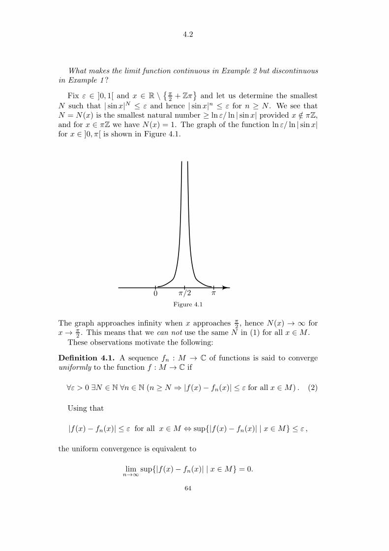
4.2

What makes the limit function continuous in Example 2 but discontinuousin Example 1 ?

Fix ε ∈ ]0, 1[ and x ∈ R \

π2+ Zπ

and let us determine the smallest

N such that | sinx|N ≤ ε and hence | sinx|n ≤ ε for n ≥ N . We see thatN = N(x) is the smallest natural number ≥ ln ε/ ln | sinx| provided x /∈ πZ,and for x ∈ πZ we have N(x) = 1. The graph of the function ln ε/ ln | sinx|for x ∈ ]0, π[ is shown in Figure 4.1.

π/20 π

Figure 4.1

The graph approaches infinity when x approaches π2 , hence N(x) → ∞ for

x→ π2 . This means that we can not use the same N in (1) for all x ∈M .

These observations motivate the following:

Definition 4.1. A sequence fn : M → C of functions is said to convergeuniformly to the function f :M → C if

∀ε > 0 ∃N ∈ N ∀n ∈ N (n ≥ N ⇒ |f(x)− fn(x)| ≤ ε for all x ∈M) . (2)

Using that

|f(x)− fn(x)| ≤ ε for all x ∈M ⇔ sup|f(x)− fn(x)| | x ∈M ≤ ε ,

the uniform convergence is equivalent to

limn→∞

sup|f(x)− fn(x)| | x ∈M = 0.

64

4.3

The functions fn(z) = zn/n! converge uniformly to the zero function for zbelonging to a bounded set M ⊆ C. The boundedness of M just means thatthere exists a constant K such that |z| ≤ K for z ∈M , and hence

sup|fn(z) − 0| | z ∈M ≤ Kn

n!→ 0 .

On the other hand, fn does not converge to the zero function uniformly forz ∈ C because

sup|fn(z)− 0| | z ∈ C =∞ for all n .

The relevance of uniform convergence for our discussion is proved in thenext theorem.

Theorem 4.2. Let M ⊆ C and let fn : M → C be uniformly convergent tothe function f :M → C.

If all the functions fn are continuous at z0 ∈M , then so is f .

Proof. Fix ε > 0. We shall determine δ > 0 such that

∀z ∈M (|z − z0| < δ ⇒ |f(z)− f(z0)| < ε) .

Since sup|f(z)− fn(z)| | z ∈M → 0 for n→∞, there exists N such that

sup|f(z)− fn(z)| | z ∈M < ε/3 for n ≥ N

in particular∀z ∈M : |f(z)− fN (z)| < ε/3 . (3)

By the continuity of fN at z0 there exists δ > 0 such that

∀z ∈M(|z − z0| < δ ⇒ |fN (z)− fN (z0)| <

ε

3

). (4)

For z ∈M such that |z − z0| < δ we then get

|f(z)− f(z0)| = |(f(z)− fN (z)) + (fN (z)− fN (z0)) + (fN (z0)− f(z0))|≤ |f(z)− fN (z)|+ |fN (z)− fN (z0)|+ |fN (z0)− f(z0)|< ε/3 + ε/3 + ε/3 = ε .

(In Theorem 4.2M could just as well be a subset of Rn or a metric space.)

65

4.4

Definition 4.3. An infinite series∑∞

0 fn(x) of functions fn : M → C issaid to converge uniformly to the sum function s :M → C if the sequence ofpartial sums

sn(x) =

n∑

k=0

fk(x) , x ∈M

converges uniformly to s.

Theorem 4.4. Weierstrass’ M-test. Let∑∞

0 fn(x) be an infinite seriesof functions fn : M → C and assume that there exists a convergent series∑∞

0 an having positive terms an such that

∀n ∈ N0 ∀x ∈M : |fn(x)| ≤ an ,

i.e. an is a majorant for fn on M for each n. Then the series∑∞

0 fn(x)converges uniformly on M .

Proof. The comparison test shows that the series∑∞

0 fn(x) is absolutelyconvergent for every x ∈M . Denoting the sum function s :M → C, the n’thpartial sum sn satisfies

s(x)− sn(x) =∞∑

k=n+1

fk(x) ,

hence

|s(x)− sn(x)| =∣∣∣

∞∑

k=n+1

fk(x)∣∣∣ ≤

∞∑

k=n+1

|fk(x)| ≤∞∑

k=n+1

ak

showing that

sup|s(x)− sn(x)| | x ∈M ≤∞∑

k=n+1

ak .

Since∑∞

0 ak <∞, the tail lemma asserts that∑∞

k=n+1 ak → 0 for n→ ∞,hence sn(x)→ s(x) uniformly on M .

Theorem 4.5. A power series∑∞

0 anzn having positive radius of conver-

gence ρ and sum function

f(z) =∞∑

n=0

anzn , z ∈ K(0, ρ)

converges uniformly to f on every closed disc K(0, r), where r < ρ.

66

4.5

(The convergence need not be uniform on K(0, ρ). The reader is supposedto be able to distinguish between the two assertions mentioned).

Proof. The result is an immediate consequence of Theorem 4.4 because∑∞0 |an|rn is a convergent series, the general term of which majorizes anz

n

on K(0, r).

We can now add a simple rule about path integrals to the rules of §2.2.Theorem 4.6. Let γ : [a, b] → C be a path in C and let fn : γ∗ → C be asequence of continuous functions.

(i) If fn → f uniformly on γ∗, then

limn→∞

∫

γ

fn =

∫

γ

f

(=

∫

γ

limn→∞

fn

).

(ii) If∑∞

n=0 fn converges uniformly on γ∗ to the sum function s : γ∗ → C,then

∞∑

n=0

∫

γ

fn =

∫

γ

s

(=

∫

γ

∞∑

n=0

fn

).

Proof. (i): Notice that f is continuous on γ∗ because of Theorem 4.2. Fixε > 0. By assumption there exists N ∈ N such that for n ≥ N and z ∈ γ∗

|f(z)− fn(z)| ≤ ε,

hence by the estimation lemma 2.8

∣∣∣∫

γ

f −∫

γ

fn

∣∣∣ =∣∣∣∫

γ

(f − fn)∣∣ ≤ εL(γ) ,

proving the assertion.

(ii): Since sn =∑n

k=0 fk converges to s uniformly on γ∗, we get by (i) that∫γsn →

∫γs, but since

∫

γ

sn =

n∑

k=0

∫

γ

fk ,

the assertion follows.

Remark 4.7. Here are two simple observations about uniform convergence.(i) If a sequence of functions fn :M → C converges uniformly to f :M →

C, then the sequence of restrictions fn|A to an arbitrary subset A ⊆ Mconverges uniformly to f |A.

67

4.6

(ii) Assume that fn : M → C converges pointwise to f : M → C andassume that A,B ⊆M .

If fn|A converges uniformly to f |A and fn|B converges uniformly to f |B,then fn|A ∪B converges uniformly to f |A ∪B.

Only the proof for (ii) requires a comment. Fixing ε > 0, the assumptionsabout uniform convergence on A and on B makes it possible to find NA ∈ N,NB ∈ N such that for n ∈ N

n ≥ NA ⇒ |f(x)− fn(x)| ≤ ε for all x ∈ A

andn ≥ NB ⇒ |f(x)− fn(x)| ≤ ε for all x ∈ B .

For n ≥ max(NA, NB) we then have

|f(x)− fn(x)| ≤ ε for all x ∈ A ∪B ,

proving the uniform convergence on A ∪B.

4.2. Expansion of holomorphic functions in power se-ries.

Let G ⊆ C be an open set. If G 6= C and a ∈ G is arbitrary, there existsa largest open disc K(a, ρ) contained in G. Its radius is given by

ρ = inf |a− z| | z ∈ C \G.

If G = C we define K(a,∞) = C, and also in this case we speak about thelargest open disc contained in G.

Using the Cauchy integral formula we shall now show that f ∈ H(G) is

differentiable infinitely often. For a ∈ G the power series∑∞

n=0f (n)(a)

n!(z−a)n

is called the Taylor series of f with centre a.

Theorem 4.8. Let f ∈ H(G). Then f is differentiable infinitely often andthe Taylor series with centre a ∈ G is convergent with sum f in the largestopen disc K(a, ρ) ⊆ G:

f(z) =

∞∑

n=0

f (n)(a)

n!(z − a)n for z ∈ K(a, ρ) . (1)

Assume that K(a, r) ⊆ G. For arbitrary z0 ∈ K(a, r) we have

f (n)(z0) =n!

2πi

∫

∂K(a,r)

f(z)

(z − z0)n+1dz , n = 0, 1, . . . , (2)

68

4.7

which is called Cauchy’s integral formula for the n’th derivative.

Proof. The function z 7→ f(z)/(z − a)n+1 being holomorphic in G \ a, itfollows by Example 3.7 that the numbers

an(r) =1

2πi

∫

∂K(a,r)

f(z) dz

(z − a)n+1

are independent of r for 0 < r < ρ. We therefore denote them briefly an ,n = 0, 1, . . . .

Fixing z ∈ K(a, ρ) and next choosing r > 0 such that |z − a| < r < ρ, weget by Cauchy’s integral formula

f(z) =1

2πi

∫

∂K(a,r)

f(w)

w − z dw .

We will prove the series expansion (1) by writing 1w−z as a sum of a conver-

gent series, insert this in the above integral formula and finally interchangesummation and integration.

First notice that for w ∈ ∂K(a, r)

1

w − z =1

w − a+ a− z =1

w − a1

1− (z − a)/(w − a) ,

and moreover |(z − a)/(w − a)| = |z − a|/r < 1, which makes it possible towrite the last fraction as the sum of a geometric series, hence

1

w − z =1

w − a

∞∑

n=0

(z − aw − a

)n

.

This shows thatf(w)

w − z =

∞∑

n=0

gn(w), (3)

where

gn(w) =f(w)(z − a)n(w − a)n+1

.

Using that ∂K(a, r) is closed and bounded, we have M = sup |f(w)| |w ∈ ∂K(a, r) < ∞. The infinite series

∑∞0 gn(w) converges uniformly for

w ∈ ∂K(a, r) by Weierstrass’ M-test because of the majorization

|gn(w)| ≤M

r

( |z − a|r

)n

,

∞∑

0

( |z − a|r

)n

<∞ .

69

4.8

By Theorem 4.6 (ii) it is allowed to integrate term by term in (3), hence

f(z) =1

2πi

∫

∂K(a,r)

f(w)

w − z dw

=

∞∑

n=0

1

2πi

∫

∂K(a,r)

gn(w) dw =

∞∑

n=0

an(z − a)n .

This shows that the power series∑∞

n=0 an(z−a)n is convergent with sumf(z) for all z ∈ K(a, ρ). Setting g(z) = f(z + a) we have g(z) =

∑∞n=0 anz

n

for z ∈ K(0, ρ). By §1.4 we know that g(z) is differentiable infinitely oftenin K(0, ρ), hence so is f(z) for z ∈ K(a, ρ). Using that the coefficients inthe power series g(z) =

∑∞n=0 anz

n are given by an = g(n)(0)/n! (cf. §1.4),we find an = f (n)(a)/n!, thereby showing (1). The formula for an = an(r),from the beginning of the proof, next shows that

f (n)(a) =n!

2πi

∫

∂K(a,r)

f(z)

(z − a)n+1dz , 0 < r < ρ .

Suppose now a ∈ K(b, s) ⊆ K(b, s) ⊆ G. If r > 0 is so small that K(a, r) ⊆K(b, s), we get by Example 3.7

f (n)(a) =n!

2πi

∫

∂K(b,s)

f(z)

(z − a)n+1dz .

This shows (2) up to a change of notation.

Remark 4.9.(i) To help memorizing the formulas observe that Cauchy’s integral formulafor the derivative follows formally from Cauchy’s integral formula by deriva-tion under the integral sign. This idea can be rigorously developed to anotherproof of Theorem 4.8.

(ii) A function f : G→ C in a domain G ⊆ C is called (complex) analytic iffor every a ∈ G there exists a power series

∑∞0 an(z − a)n with sum f(z) in

a suitable disc K(a, r) ⊆ G, where r is allowed to vary with a. By §1.4 ananalytic function is holomorphic, and Theorem 4.8 shows that a holomorphicfunction is analytic. Moreover, the power series attached to the point a isthe Taylor series. The two concepts “analytic” and “holomorphic” are thusequivalent. K. Weierstrass (1815–1897) gave the first rigorous treatment ofcomplex function theory based on the concept of an analytic function.

(iii) Since f ′ is again holomorphic, we have proved that f ′ is in particular acontinuous function, cf. the preamble to Goursat’s lemma.

70

4.9

(iv) The radius of convergence R for the power series in (1) is ≥ ρ. It canhappen that R > ρ. See Theorem 6.24 for a case where R = ρ.

4.3. Harmonic functions.

Consider two differentiable functions u, v : G→ R satisfying the Cauchy-Riemann differential equations in the open set G ⊆ R2

∂u

∂x=∂v

∂y,

∂u

∂y= −∂v

∂xin G .

Using that f = u + iv is holomorphic and hence differentiable infinitelyoften, we see the very surprising phenomenon that u, v are automaticallyC∞-functions in G. Differentiating once more we find

∂2u

∂x2=

∂2v

∂x∂y,

∂2u

∂y2= − ∂2v

∂y∂x

hence∂2u

∂x2+∂2u

∂y2= 0 because

∂2v

∂x∂y=

∂2v

∂y∂x.

In an analogous way we see that∂2v

∂x2+∂2v

∂y2= 0.

The expression∂2

∂x2+

∂2

∂y2is called the Laplace operator and is usually

written , i.e. ϕ =∂2ϕ

∂x2+∂2ϕ

∂y2.

A real-valued C2-function ϕ defined on an open set G ⊆ R2 is calledharmonic in G, if ϕ = 0 in G. We have thus proved: The real part and theimaginary part of a holomorphic function are harmonic.

The opposite is true locally. More precisely we will prove:

Theorem 4.10. Let u be a harmonic function in a simply connected domainG ⊆ R2 ≈ C. Then there exists a holomorphic function f : G→ C such thatRe f = u, and f is uniquely determined up to addition of a purely imaginaryconstant.

Proof. The function g(z) =∂u

∂x− i∂u

∂yis holomorphic in G, because we can

verify the Cauchy-Riemann equations:

∂2u

∂x2= −∂

2u

∂y2,

∂2u

∂y∂x=

∂2u

∂x∂y.

By Theorem 3.5 there exists a primitive h ∈ H(G) to g, i.e. h′ = g (here wehave used that G is simply connected). Moreover

h′ =∂

∂x(Reh) + i

∂

∂x(Imh) =

∂

∂x(Reh)− i ∂

∂y(Reh),

71

4.10

and we therefore get

∂

∂x(Reh) =

∂u

∂x,

∂

∂y(Reh) =

∂u

∂y,

showing that u−Re h is a real constant, which we call c. Then f = h+ c is aholomorphic function having u as its real part. If f and f1 are holomorphicfunctions such that Re f = Re f1 = u, then i(f − f1) is a real-valued holo-morphic function, hence constant by Corollary 1.10.

Given a harmonic function u in a simply connected domain G ⊆ R2,there exists, as we have seen, another harmonic function v in G such thatf = u+iv is holomorphic. The function v is only determined up to addition ofa constant. We call v a conjugate harmonic function to u. As an example thefunctions u(x, y) = x and v(x, y) = y are harmonic in R2 and v is conjugateto u because z = u + iv is holomorphic. Also x and y + c are conjugateharmonic functions for any real c.

If u is harmonic in an open set G, then for any disc K(a, r) ⊆ G thereexists a conjugate harmonic function v to u in the disc because it is simplyconnected. Using that u + iv is holomorphic in K(a, r), we see that u ∈C∞(G).

We thus have the remarkable result: Suppose that u ∈ C2(G) satisfiesu = 0. Then u ∈ C∞(G).

This result is a real-valued counterpart to the complex analysis result thata holomorphic function is differentiable infinitely often.

4.4. Morera’s theorem and local uniform convergence.

In real analysis we know that every continuous function on an interval hasa primitive. In complex function theory the situation is completely different:

Theorem 4.11. If a function f : G → C on an open set G ⊆ C has aprimitive, then it is holomorphic.

Proof. If F ∈ H(G) is a primitive of f , then also f = F ′ is holomorphic byTheorem 4.8.

We recall that a holomorphic function in a domain G need not have aprimitive in G, (Example 2.14, f(z) = z−1 in C \ 0), but if G is assumedto be simply connected a primitive always exists, cf. Theorem 3.5.

The following theorem from 1886 by the Italian mathematician G. Morerais a converse to the integral theorem of Cauchy. Notice that the domain ofdefinition need not be simply connected but can be any open set.

72

4.11

Theorem 4.12. Morera’s theorem. Let f : G → C be continuous in anopen set G ⊆ C. If

∫γf = 0 for every closed path γ in G, or if only

∫∂ f = 0

for every solid triangle ⊆ G, then f is holomorphic in G.

Proof. Fix a ∈ G. It is enough to prove that f is holomorphic in the largestopen discK(a, ρ), contained in G. For a solid triangle contained inK(a, ρ)we get by assumption

∫∂ f = 0, and as in the proof of Cauchy’s integral

theorem for a star-shaped domain we conclude that the integral of f alongevery closed staircase line in K(a, ρ) equals 0, hence f has a primitive inK(a, ρ). By Theorem 4.11 we now get that f is holomorphic in K(a, ρ).

We shall now recall a fundamental result in mathematical analysis andtopology.

Theorem 4.13. Borel’s covering theorem. Let K be a closed andbounded subset of C.

To every family (Gi)i∈I of open sets in C covering K, i.e.

K ⊆⋃

i∈I

Gi,

there exist finitely many indices i1, . . . , in ∈ I such that

K ⊆ Gi1 ∪ · · · ∪Gin .

(In the statement C can be replaced by Rk.)

We shall use this result in connection with a new concept of convergencefor sequences of functions, particularly relevant for holomorphic functions.

Definition 4.14. Let G ⊆ C be an open set. A sequence of functionsfn : G→ C is said to converge locally uniformly to a function f : G→ C if

(lu) To every a ∈ G there exists r > 0 such that K(a, r) ⊆ G and fn(z)→f(z) uniformly for z ∈ K(a, r).

If (lu) holds we have in particular fn(a) → f(a) for every a ∈ G, i.e.fn → f pointwise, and the convergence is assumed to be uniform in a suitableneighbourhood of every point in G. The question arises for which class ofsets K ⊆ G uniform convergence holds.

Theorem 4.15. Let G ⊆ C be an open set. A sequence of functions fn :G→ C converges locally uniformly to f : G→ C if and only if the followingcondition holds

(cu) For every closed and bounded set K ⊆ G we have fn(z) → f(z)uniformly for z ∈ K.

73

4.12

Proof. (lu) ⇒ (cu). Let K ⊆ G be closed and bounded. For every a ∈ Kthere exists r = ra > 0 such that K(a, ra) ⊆ G and fn → f uniformly on

K(a, ra). The discs (K(a, ra))a∈K are open and they cover K, because eacha ∈ K lies in the disc K(a, ra). By the covering theorem of Borel there existfinitely many points a1, . . . , an ∈ K such that

K ⊆ K(a1, ra1) ∪ · · · ∪K(an, ran

) .

The sequence (fn) being uniformly convergent on each of these discs, Re-mark 4.7 shows that fn → f uniformly on K.

(cu) ⇒ (lu). Fix a ∈ G. We have to find a disc K(a, r) ⊆ G, such that

fn converges uniformly to f on K(a, r). However, K(a, r) being closed andbounded, the uniform convergence on every such disc in G has been estab-lished.

Remark 4.16. The condition (cu) is an abbreviation for “compact-uniform”convergence, because closed and bounded subsets of C (or Rk) are oftencalled compact. The condition thus reads that the convergence is uniformon every compact subset of G. We have seen that uniform convergence in aneighbourhood (no matter how small) of every point in the open set impliesuniform convergence on arbitrary compact subsets of G.

We shall use Morera’s theorem to prove the following:

Theorem 4.17. Let G ⊆ C be open. If a sequence f1, f2, . . . from H(G)converges locally uniformly in G to a function f , then f ∈ H(G), and thesequence f ′

1, f′2, . . . of derivatives converges locally uniformly in G to f ′.

Remark 4.18. By repeated application of the theorem we see that f(p)n →

f (p) locally uniformly in G for every p ∈ N.

Proof. Let a ∈ G andK(a, r) ⊆ G be such that fn → f uniformly onK(a, r).By Theorem 4.2 f is continuous at every point of K(a, r). For every triangle ⊆ K(a, r) we have

∫∂ fn = 0 by Cauchy’s integral theorem. Since fn → f

uniformly on ∂, we get

0 =

∫

∂fn →

∫

∂f

by Theorem 4.6 (i), hence∫∂ f = 0. By Morera’s theorem f is holomorphic

in K(a, r), and a being arbitrary, we have proved that f ∈ H(G).

74

4.13

By Cauchy’s integral formula for the derivative we get for z0 ∈ K(a, r)

f ′n(z0)− f ′(z0) =

1

2πi

∫

∂K(a,r)

fn(z)− f(z)(z − z0)2

dz .

For z0 ∈ K(a, r/2) and z ∈ ∂K(a, r) we have |(z − z0)2| ≥ (r/2)2, hence

|f ′n(z0)− f ′(z0)| ≤

2πr

2π

(2

r

)2

supz∈∂K(a,r)

|fn(z)− f(z)| ,

which yields

supz0∈K(a,r/2)

|f ′n(z0)− f ′(z0)| ≤

4

rsup

z∈∂K(a,r)

|fn(z)− f(z)| .

This shows that f ′n → f ′ uniformly onK(a, r/2), and since a ∈ G is arbitrary

we have proved that f ′n → f ′ locally uniformly in G.

Corollary 4.19. Let G ⊆ C be open. Let f0, f1, . . . be a sequence of holo-morphic functions on G and assume that the infinite series

s(z) =

∞∑

k=0

fk(z), z ∈ G (1)

converges locally uniformly on G to a function s : G → C. Then s ∈ H(G)and the series can be differentiated term by term infinitely often

s(p)(z) =∞∑

k=0

f(p)k (z), z ∈ G, p = 1, 2, . . . , (2)

and each of these series converges locally uniformly on G.

Proof. By Definition 4.3 the sequence of partial sums

sn(z) =

n∑

k=0

fk(z)

converges locally uniformly on G to s(z), and since sn ∈ H(G) we conclude byTheorem 4.17 that s ∈ H(G). Furthermore, s′n(z) converges locally uniformlyto s′(z), i.e.

s′(z) =∞∑

k=0

f ′k(z),

75

4.14

which is (2) for p = 1. Formula (2) follows by repeated applications of theresult.

Theorem 1.12 about differentiation term by term of a power series is ofcourse a special case of Corollary 4.19.

Since an integral is a limit of finite sums, it is to be expected that anexpression of the form

F (z) =

∫ b

a

f(x, z) dx

is holomorphic, if f(x, z) is holomorphic in z for each x. We give a precisestatement.

Theorem 4.20. Let G ⊆ C be open and let f : [a, b]×G→ C be a continuousfunction such that f(x, ·) ∈ H(G) for each x ∈ [a, b]. Then

(i) ∂nf∂zn : [a, b]×G→ C is continuous for n = 1, 2, . . . ,

(ii) F (z) =∫ b

af(x, z) dx is holomorphic in G,

and for n = 1, 2, . . .

F (n)(z) =

∫ b

a

∂nf

∂zn(x, z) dx, z ∈ G (3)

Proof. (a) We prove first that ∂f∂z is continuous at (x0, z0) ∈ [a, b] × G.

Choose r > 0 such that K(z0, r) ⊆ G. For x ∈ [a, b], z ∈ K(z0, r) wehave by Cauchy’s integral formula for the derivative

∂f

∂z(x, z) =

1

2πi

∫

∂K(z0,r)

f(x, w)

(w − z)2 dw. (4)

The function G(x, z, w) = f(x, w)/(w−z)2 is continuous on [a, b]×K(z0, r)×∂K(z0, r). Applying Theorem A.7 with A = [a, b] × K(z0, r) and B =∂K(z0, r), we see that for given ε > 0

∣∣∣∣f(x, w)

(w − z)2 −f(x0, w)

(w − z0)2∣∣∣∣ < ε for all w ∈ ∂K(z0, r) (5)

provided (x, z) is sufficiently close to (x0, z0). For (x, z) such that (5) holds,it follows by (4) and by the estimation lemma 2.8 that

∣∣∣∣∂f

∂z(x, z)− ∂f

∂z(x0, z0)

∣∣∣∣ ≤ rε,

hence that ∂f∂z is continuous at (x0, z0).

76

4.15

(b) We next prove (ii) and (3) for n = 1. For g ∈ H(G) and K(z0, r) ⊆ Gwe have for |h| < r

g(z0 + h)− g(z0) =∫ 1

0

d

dtg(z0 + th) dt = h

∫ 1

0

g′(z0 + th) dt.

Applying this to g(z) = f(x, z) for each x ∈ [a, b] we get

f(x, z0 + h)− f(x, z0) = h

∫ 1

0

∂f

∂z(x, z0 + th) dt,

hence by integrating over [a, b]

1

h(F (z0 + h)− F (z0)) =

∫ b

a

(∫ 1

0

∂f

∂z(x, z0 + th) dt

)dx, 0 < |h| < r.

By (i) for n = 1 the function (h, x, t) → ∂f∂z

(x, z0 + th) is continuous onK(0, r)× [a, b]× [0, 1]. Given ε > 0 we see by Theorem A.7 that∣∣∣∣

∂f

∂z(x, z0)−

∂f

∂z(x, z0 + th)

∣∣∣∣ < ε,

for all x ∈ [a, b], t ∈ [0, 1], provided |h| < δ for a sufficiently small δ > 0. Thisgives for 0 < |h| < δ∣∣∣∣∣

∫ b

a

∂f

∂z(x, z0) dx−

1

h(F (z0 + h) − F (z0))

∣∣∣∣∣

=

∣∣∣∣∣

∫ b

a

(∫ 1

0

(∂f

∂z(x, z0)−

∂f

∂z(x, z0 + th)

)dt

)dx

∣∣∣∣∣ ≤ ε(b− a),

which shows that F is complex differentiable at z0 with

F ′(z0) =

∫ b

a

∂f

∂z(x, z0) dx.

Since ∂f∂z (x, ·) ∈ H(G) for each x ∈ [a, b], we can apply to ∂f

∂z what we havealready proved. This gives (i) and (3) for n = 2. It is clear the the processcan be repeated to give (i) and (3) for all n.

4.5. Entire functions. Liouville’s theorem.

A holomorphic function f : C→ C is called an entire function. Polynomi-als, exp , sin , cos , sinh , cosh are entire functions, but 1

z is not entire. Foran entire function the formula (1) of Theorem 4.8 holds for all z, a ∈ C andin particular for a = 0. The study of entire functions is therefore equivalentwith the study of power series with infinite radius of convergence. We canthink informally of entire functions as “polynomials of infinite degree”.

There is a long list of deep and interesting theorems about entire functions.We mention the following without proof:

77

4.16

Theorem 4.21. Picard’s theorem. Let f : C → C be a non-constantentire function. Then either f(C) = C or f(C) = C\a for a suitable pointa ∈ C. If f is different from a polynomial, then for all w ∈ C with at mostone exception, the equation f(z) = w has infinitely many solutions z.

As illustration of the theorem take f(z) = exp z. The equation exp z = whas no solutions when w = 0, but for w 6= 0 there is infinitely many solutions.More about this will be discussed in Section 5.4.

Picard’s theorem shows that a bounded entire function is constant. Wegive a complete proof of this result which is known as Liouville’s theorem.

Theorem 4.22. Liouville’s theorem. A bounded entire function is con-stant.

Proof. Assume that f is an entire function such that |f(z)| ≤ M for allz ∈ C. By Cauchy’s integral formula for the derivatives we get for any r > 0

∣∣f (n)(0)∣∣ =

∣∣ n!2πi

∫

∂K(0,r)

f(z)

zn+1dz∣∣ ≤ n!

2π

M

rn+12πr =

M · n!rn

.

Letting r →∞ (which is possible because f is entire), we see that f (n)(0) = 0for all n ≥ 1, and the assertion follows from the Taylor expansion of f .

4.6. Polynomials.

Liouville’s theorem is quite deep, although it is simple to prove. The depthis illustrated by the following application:

Theorem 4.23. The fundamental theorem of algebra. Every poly-nomial p(z) =

∑nk=0 akz

k of degree n ≥ 1 has at least one zero (=root) inC.

Proof. Assuming p(z) 6= 0 for all z ∈ C, we see that f(z) = 1/p(z) must bean entire function.

By the assumption of p being of degree n we have an 6= 0, which allowsus to write

p(z) = anzn

(1 +

n−1∑

k=0

akanzk−n

),

hencep(z)

anzn→ 1 for |z| → ∞ .

78

4.17

By this result there exists r > 0 such that

∣∣∣∣p(z)

anzn

∣∣∣∣ ≥1

2for |z| ≥ r

or1

|p(z)| ≤2

|an|rnfor |z| ≥ r .

The continuous function 1/|p(z)| is also bounded on the closed and bounded

set K(0, r), hence 1/p is a bounded entire function and finally constant byLiouville’s theorem. This contradiction shows that p has at least one zero.

For the set of polynomials

p(z) = a0 + a1z + · · ·+ anzn

with complex coefficients we use the standard notation C[z] from algebra.We recall the following fundamental result about division of polynomials:

Theorem 4.24. Let d ∈ C[z] be different from the zero polynomial. Top ∈ C[z] there exist uniquely determined polynomials q, r ∈ C[z] such that

p = qd+ r , deg(r) < deg(d).1) (1)

If d, p have real coefficients, then so have q, r.

The polynomials d, q, r are called divisor, quotient and remainder respec-tively.

Proof. To see the uniqueness statement let p = q1d + r1 = q2d + r2 wheredeg(rj) < deg(d), j = 1, 2. By subtraction we get (q1− q2)d = r2− r1, whichis a polynomial of degree < deg(d), but this is only possible if q1 − q2 = 0,and then we also have r1 = r2.

The existence can be seen by induction in deg(p). If deg(p) < deg(d) theexistence is clear by defining q = 0, r = p. Assume next that we have provedthe existence for deg(p) ≤ n− 1, and let us prove it for deg(p) = n. Callingdeg(d) = k, we can write

p(z) = anzn + · · ·+ a0 , d(z) = bkz

k + · · ·+ b0,

where an 6= 0, bk 6= 0. As already seen, we can assume n ≥ k.

1) The zero polynomial is assigned the degree −∞

79

4.18

The polynomial

p1(z) =p(z) −anbkzn−kd(z) =

an−1zn−1 + · · ·+ a0 −

anbk

(bk−1z

n−1 + · · ·+ b0zn−k

)

has degree ≤ n − 1, so by the induction hypothesis we can find polynomialsq1, r1 such that

p1 = q1d+ r1 , deg(r1) < deg(d) ,

hence

p(z) = p1(z) +anbkzn−kd(z) =

(q1(z) +

anbkzn−k

)d(z) + r1(z) .

Example 4.25. p(z) = 2z3 + 3z2 + z + 3, d(z) = z2 − z + 1

z2 − z + 1∣∣∣2z3 + 3z2 + z + 3

∣∣∣ 2z + 5

2z3 − 2z2 + 2z

5z2 − z + 3

5z2 − 5z + 5

4z − 2

This gives q(z) = 2z + 5, r(z) = 4z − 2.

Example 4.26. Let d(z) = z − a be of degree one. The theorem yieldsp(z) = q(z)(z − a) + r, where r ∈ C. Inserting z = a gives r = p(a). A zeroz = a of p therefore leads to the factorization p(z) = q(z)(z − a).

A repeated use of this gives

Corollary 4.27. A polynomial p(z) of degree n ≥ 1 has precisely n zerosin C counted with multiplicity. Denoting z1, . . . , zk the different zeros of phaving the multiplicities n1, . . . , nk respectively, we have

p(z) = an(z − z1)n1 · · · (z − zk)nk ,

where an is the leading coefficient.

Proof. For n = 1 the theorem is trivial. Assume that we have proved theCorollary for polynomials of degree n−1 and let us prove it for a polynomialp of degree n > 1. By Theorem 4.23 we can factorize p(z) = (z − z1)q(z)for some zero z1 of p. Since q has degree n − 1 we know by the inductionhypothesis that it has n− 1 zeros counted with multiplicity. Therefore p hasn zeros. The given factorization also follows by induction.

80

4.19

Exercises for §4.

4.1. Let G be an open subset of C and let a ∈ G. Assume that f ∈ H(G)satisfies f ′(a) 6= 0.

Prove that there exists r > 0, such that |f ′(z) − f ′(a)| < |f ′(a)| forz ∈ K(a, r) ⊆ G. Show next that

∣∣∫ 1

0

f ′(tz2 + (1− t)z1)dt− f ′(a)∣∣ < |f ′(a)| ,

f(z2)− f(z1) = (z2 − z1)∫ 1

0

f ′(tz2 + (1− t)z1) dt ,

for arbitrary z1, z2 ∈ K(a, r), and deduce that f |K(a, r) is one-to-one.In summary we have proved: f is one-to-one in a sufficiently small neigh-

bourhood of a point a for which f ′(a) 6= 0.Give an example of an entire function f which is not one-to-one but such

that f ′(z) 6= 0 for all z ∈ C.

4.2. Find the Taylor series with centre π/4 for the sine function in the fol-lowing two ways: (i) Use the addition formula. (ii) Determine the coefficientsby differentiation.

4.3. What is the largest domain G ⊆ C for which f(z) = 1/(1− z + z2) isholomorphic? Show that f(z) =

∑∞0 anz

n for |z| < 1, and that a0 = a1 = 1 ,a2 = 0, and an+3 = −an for n ≥ 0.

Hint. Use that 1 = (1− z + z2)∑∞

0 anzn and apply Theorem 1.14.

4.4. Determine the value of

∫

∂K(i,2)

ez

(z − 1)ndz for n ≥ 1 .

4.5. Let u : G→ R be a harmonic function in an open set G ⊆ C. AssumingK(a, r) ⊆ G, show that

u(a) =1

2π

∫ 2π

0

u(a+ reiθ) dθ .

4.6. Show that

u(x, y) =x

x2 + y2and u(x, y) = x2 − y2

81

4.20

are harmonic functions in R2 \ (0, 0) respectively R2, and find conjugateharmonic functions.

4.7. Let (fn) be a sequence of holomorphic functions in an open set G andassume that ∞∑

n=1

supK|fn(z)| <∞,

for every closed and bounded set K ⊆ G. Show that

f(z) =

∞∑

n=1

fn(z)

is holomorphic in G, and that f ′(z) =∑∞

1 f ′n(z), where the series converges

locally uniformly on G.

4.8. Let K and L be closed and bounded sets in C such that K 6= ∅ and

K ⊆L, and let d denote the distance between K and C \

L, i.e.

d = inf |z − w| | z ∈ K , w ∈ C \L .

Explain why d > 0 and prove that for every open set G ⊇ L and for everyf ∈ H(G)

supK|f ′(z)| ≤ 1

dsupL|f(z)| .

Hint. Explain why it is possible to apply Cauchy’s integral formula

f ′(a) =1

2πi

∫

∂K(a,d)

f(ξ)

(ξ − a)2 dξ for a ∈ K .

4.9. Let f be an entire function and assume that

|f(z)| ≤ A+B|z|n for z ∈ C ,

where A,B ≥ 0 and n ∈ N. Prove that f is a polynomial of degree ≤ n.

4.10. Let f be a non-constant entire function. Prove (without referring to

Picard’s Theorem) that f(C) = C.

Hint. Assume that f(C) 6= C, and try to apply Liouville’s theorem.

4.11. Let f be an entire function satisfying f ′ = af for some a ∈ C. Showthat there exists c ∈ C such that

f(z) = c exp(az) , z ∈ C .

82

4.21

4.12. Let ϕ ∈ H(G). Show that the infinite series

f(z) =

∞∑

n=1

sin

(ϕ(z)

n2

)

defines a holomorphic function in G.

4.13. (Requires basic measure theory). Let (X,E, µ) be a measurable spaceand let G ⊆ C be open. Assume that f : X ×G→ C satisfies

(i) ∀x ∈ X : f(x, ·) ∈ H(G).(ii) ∀z ∈ G : f(·, z) is measurable on X .(iii) There exists a measurable function g : X → [0,∞] satisfying

∫g dµ <

∞, such that

|f(x, z)| ≤ g(x) for x ∈ X , z ∈ G .

1. Prove that ∂f∂z

(·, z) is measurable for each z ∈ G.2. Assume that K(z0, r) ⊆ G. Prove that

∣∣∣∣∂f

∂z(x, z)

∣∣∣∣ ≤4

rg(x), z ∈ K(z0, r/2), x ∈ X.

and that

1

h(f(x, z0 + h) − f(x, z0)) =

∫ 1

0

∂f

∂z(x, z0 + th) dt, 0 < |h| < r, x ∈ X.

3. Prove that

F (z) =

∫

X

f(x, z) dµ(x), z ∈ G,

is holomorphic in G and

F ′(z) =

∫

X

∂f

∂z(x, z) dµ(x), z ∈ G.

Remark. Notice that (iii) can be replaced by local conditions: For eacha ∈ G there exist a disc K(a, r) ⊆ G and a “majorant” g, both dependingon a such that

|f(x, z)| ≤ g(x) for x ∈ X, z ∈ K(a, r).

83

4.22

Notice also that in this version the results can be applied to ∂f∂z , so the

final conclusion is that we can differentiate the integral infinitely often bydifferentiating under the integral sign:

F (n)(z) =

∫∂n

∂zn(x, z) dµ(x), z ∈ G, n ∈ N.

4.14. Explain why the power series∑∞

n=0 zn converges uniformly to 1

1−z

for z ∈ K(0, r) for every r < 1. Prove that the series does not convergeuniformly on K(0, 1).

4.15. Let p(z) = a0 +a1z+ · · ·+anzn be a polynomial of degree n ≥ 1 withreal coefficients. Prove that if z = a is a zero of p, then so is z = a and of thesame multiplicity as a. Prove that if n is odd, then p has at least one realzero.

4.16. Assume that f ∈ H(K(0, r)) has the power series

f(z) = 1 + a1z + a2z2 + · · · for |z| < r .

Prove that there exists ρ > 0 such that 1/f ∈ H(K(0, ρ)) and that thecoefficients (bn) in the power series

1

f(z)=

∞∑

n=0

bnzn , |z| < ρ

satisfy

b0 = 1 , b1 = −a1 , b2 = a21 − a2 .

4.17. Let p(z) =∑n

k=0 an−kzk be a polynomial of degree n ≥ 1, i.e. a0 6= 0,

and assume that an−k = ak, k = 0, 1, . . . , n.Prove that if z is a zero of p, then z 6= 0 and 1/z is also a zero of p.Find the zeros of the polynomial 2z4 − 3z3 − z2 − 3z + 2.Hint. z = 2 is a zero of p.

4.18. Show that the functions

u(x, y) = ex cos y, u(x, y) = sinx cosh y, u(x, y) = cosx cosh y

are harmonic in R2 and find entire functions having u as real part.

84

4.23

4.19. Prove that the series∞∑

n=1

1

nz(nz := exp(z lnn), z ∈ C)

is absolutely convergent for all z ∈ C with Re z > 1, and that the sum

ζ(z) =

∞∑

n=1

1

nz, Re z > 1

defines a holomorphic function in the open half-plane Re z > 1. This is thefamous Riemann zeta function.

Let p1 = 2, p2 = 3, p3 = 5, . . . denote the sequence of prime numbers.Prove that

∣∣∣∣∣ζ(z)N∏

k=1

(1− 1

pzk

)− 1

∣∣∣∣∣ ≤∞∑

n=pN+1

1

nRe z, Re z > 1,

and conclude that ζ(z) 6= 0 and

limN→∞

N∏

k=1

(1− 1

pzk

)=

1

ζ(z), Re z > 1.

4.20. (i) Prove that

f(t) =

−t ln t , 0 < t ≤ 1

0 , t = 0

is a continuous function on [0, 1] and∫ 1

0

(f(t))n dt =n!

(n+ 1)n+1, n = 0, 1, . . . .

Hint. Use or prove by induction that∫∞0xn exp(−x) dx = n!.

(ii) Prove that

F (z) =

∫ 1

0

exp(zf(t)) dt, z ∈ C

is an entire function with the power series

F (z) =∞∑

n=0

zn

(n+ 1)n+1, z ∈ C.

(iii) Prove that

F (1) =

∫ 1

0

dt

tt=

∞∑

n=1

1

nn.

85

4.24

Karl Weierstrass (1815–1897), German

86

5.1

§5. Argument. Logarithm. Powers

This section is focusing on the concept of argument of a complex number.The argument being only determined modulo 2π, it is important to be able tochoose the argument in such a way that it depends continuously on the pointsin question. It turns out that we can choose the argument in a continuousway in two situations: For the points along a continuous curve in C \ 0(Theorem 5.10), and for the points in a simply connected domain G ⊆ C\0(Theorem 5.15). Notice that in both cases we have to avoid the point zero,where the argument is not defined.

To prove these results we have to discuss the concept of path connected-ness from general topology, thereby bringing our preliminary definition of adomain in accordance with the definitions of general topology.

Using a continuously varying argument along a continuous curve, we candefine precisely how many times it winds around zero. This is the windingnumber.

Logarithms, n’th roots and powers of arbitrary exponent are multi-valuedfunctions. We examine how we can choose branches of these functions suchthat they become ordinary holomorphic functions.

There is another way of treating multi-valued functions, going back to Rie-mann. We stack copies (layers) of the complex plane and glue them togetheralong certain curves such that it becomes possible to move from one layerto the next. All the layers are then viewed as one entity called a Riemannsurface. This is only an inaccurate picture. If the multi-valued function hasn values (n = 2, 3, . . . ,∞) at a point z0 ∈ C we shall stack n layers overthat point. We will only discuss the most simple example

√z, which needs a

Riemann surface with two layers. The theory of Riemann surfaces is compre-hensive and complicated and has been a source of inspiration for the generaltheory of differentiable manifolds.

5.1. Some topological concepts.

All definitions and results in this subsection 5.1 are formulated for thecomplex plane, but could just as well have been formulated for Rk.

Definition 5.1. A subset A ⊆ C is called path connected, if two arbitrarypoints from A can be connected by a continuous curve contained in A.

In other words, given P,Q ∈ A there exists a continuous function γ :[0, 1]→ C such that γ(0) = P , γ(1) = Q and γ(t) ∈ A for all t ∈ [0, 1].

If a set A ⊆ C is star-shaped with respect to P0 ∈ A, then A is pathconnected.

87

5.2

We first notice that an arbitrary point P ∈ A is connected to P0 by theline segment γ(t) = (1− t)P0 + tP . If δ is a similar line segment from P0 toQ ∈ A, then −γ ∪ δ defines a continuous curve from P to Q.

In particular every convex set is path connected.Every domain is path connected, since two arbitrary points can be con-

nected by a staircase line, cf. Definition 1.8.A circle is path connected but it is of course not possible to connect two

different points on the circle by a staircase line.We will prove that in a path connected open subset of C there is enough

space to make it possible to connect any two points by a staircase line.As a preparation we prove a useful result called the “paving lemma”,

because it “shows” that a garden path can be covered by a finite number ofcircular flagstones of the same size (although we allow them to be overlappingcontrary to reality).

5.2. The paving lemma. Let G be an open subset of C and let γ : [a, b]→G be a continuous curve in G.

There exist finitely many points a = t0 < t1 < · · · < tn = b in the interval[a, b] and a radius r > 0 such that

n⋃

i=0

K(γ(ti), r) ⊆ G (1)

and

γ([ti, ti+1]) ⊆ K(γ(ti), r) , i = 0, 1, · · · , n− 1 . (2)

Proof. By a main theorem of analysis γ is uniformly continuous. Givenε = r > 0, there exists δ > 0 such that |γ(t)− γ(s)| < r provided t, s ∈ [a, b]satisfy |t− s| ≤ δ. We now divide the interval [a, b] by finitely many pointsti as above such that ti+1 − ti ≤ δ for each i. Then (2) clearly holds. IfG = C, then (1) holds for any r > 0. The set γ([a, b]) is closed and bounded,cf. Theorem A.3. If G 6= C, there is a positive distance d between γ([a, b])and the closed set C \ G, cf. Lemma A.1. By choosing r < d both (1) and(2) hold provided δ > 0 is chosen in accordance with the uniform continuitycorresponding to ε = r.

Theorem 5.3. An open path connected set G ⊆ C is a domain5 in the sensethat any two points in G can be connected by a staircase line belonging to G.

Proof. Let P,Q ∈ G and let γ : [0, 1]→ C be a continuous curve in G fromP to Q. By the paving lemma there exist points 0 = t0 < · · · < tn = 1 andr > 0 such that (1) and (2) hold.

5Recall Definition 1.8

88

5.3

In a disc K(a, r) an arbitrary point P ∈ K(a, r) can be connected to thecentre a by a staircase line consisting of at most two line segments. We arenow able to construct a staircase line from γ(0) = P to γ(1) = Q by firstmoving to γ(t1) in the disc K(γ(0), r), next moving from γ(t1) to γ(t2) inthe disc K(γ(t1), r), next moving from γ(t2) to γ(t3) in the disc K(γ(t2), r)and so on. Because of (1), the total staircase line is contained in G.

Definition 5.4. Let A ⊆ C be given. A point a ∈ C is called an accumula-tion point or a cluster point of A if

∀r > 0 : K ′(a, r) ∩A 6= ∅ .

In other words, it shall be possible to find points x ∈ A which are arbitrarilyclose to a but different from a. This is equivalent to the existence of asequence xn ∈ A \ a such that xn → a for n → ∞. A point a ∈ A, whichis not an accumulation point of A, is called isolated in A. It is characterizedby the requirement

∃r > 0 : K(a, r) ∩ A = a .

Definition 5.5. Let G ⊆ C be open. A set A ⊆ G is called discrete in G, ifA has no accumulation points in G.

Examples. For A = R and for A = Q the accumulation points are preciselythe points of R. The set A = Z or an arbitrary set A ⊆ Z is discrete in C.The set A =

1n| n ∈ N

is discrete in C \ 0, but 0 is an accumulation

point of A.

Theorem 5.6. Let G ⊆ C be open. A discrete set A ⊆ G is countable (seeA.9) and G \A is open.6

Proof. An arbitrary point a ∈ G is not an accumulation point of A, hencethere exists r = ra > 0 such that

K ′(a, ra) ∩ A = ∅ . (3)

We can also assume that K(a, ra) ⊆ G, for otherwise we just replace ra by asmaller radius.

If a ∈ G\A we even have K(a, ra)∩A = ∅, hence K(a, ra) ⊆ G\A. Thisshows that G \A is open.

If a ∈ A we haveK(a, ra) ∩A = a . (4)

Let nowK ⊆ G be a closed and bounded set. The discs K(a, ra) | a ∈ Kform an open covering of K. By Borel’s covering theorem 4.13, we can finda1, . . . , an ∈ K such that

K ⊆ K(a1, ra1) ∪ . . . ∪K(an, ran

) ,

6We can also say that A is closed relative to G.

89

5.4

hence

A ∩K ⊆n⋃

i=1

A ∩K(ai, rai) ⊆ a1, . . . , an .

This shows that A ∩K is a finite set.We finish the proof by making use of the following important fact: There

exists a sequence K1 ⊆ K2 ⊆ · · · of closed and bounded subsets of G ex-hausting G, i.e. having G as their union, cf. Theorem A.5.

Therefore A is the union of the finite sets A∩Kn, n = 1, 2, . . . and hencecountable by Theorem A.11.

Theorem 5.7. Let f : A → C be a continuous function defined on a pathconnected set A ⊆ C, and assume that f(A) is discrete in C.

Then f is constant.

Proof. Fix P0 ∈ A. We shall prove that f(P ) = f(P0) for arbitrary P ∈ A.To P ∈ A we choose a continuous curve γ : [0, 1]→ C such that γ(0) = P0,γ(1) = P and γ(t) ∈ A for t ∈ [0, 1].

Since f(A) is discrete in C, there exists r > 0 such that

K(f(P0), r) ∩ f(A) = f(P0),

cf. (4), but f γ : [0, 1]→ C being continuous at 0, there exists δ0 > 0 suchthat

∀t ∈ [0, 1] : 0 ≤ t ≤ δ0 ⇒ |f(γ(t))− f(γ(0))| < r,

hence0 ≤ t ≤ δ0 ⇒ f(γ(t)) ∈ K(f(P0), r) ∩ f(A) = f(P0) .

This shows that f(γ(t)) is equal to f(P0) for t ∈ [0, δ0]. The idea is nowroughly speaking that since f(γ(δ0)) = f(P0), an argument as before provesthat f(γ(t)) = f(P0) for t ∈ [δ0, δ0 + δ] for a sufficiently small δ, and after afinite number of steps we reach t = 1. However, one can fear that each newstep δ can be smaller and smaller in such a way that we never reach t = 1.We therefore have to be more precise.

DefineE = t ∈ [0, 1] | ∀s ∈ [0, t] : f(γ(s)) = f(P0) .

We have seen that [0, δ0] ⊆ E, and defining t0 := supE we get δ0 ≤ t0 ≤ 1.Since f(A) is assumed to be discrete in C we know that f(γ(t0)) is not an

accumulation point of f(A). Therefore, there exists r > 0 such that

K(f(γ(t0)), r) ∩ f(A) = f(γ(t0)) ,

cf. (4), and f γ being continuous at t0, there exists δ > 0 such that

∀t ∈ [0, 1] : t0 − δ ≤ t ≤ t0 + δ ⇒ |f(γ(t))− f(γ(t0))| < r,

90

5.5

hencet ∈ [0, 1] ∩ [t0 − δ, t0 + δ]⇒ f(γ(t)) = f(γ(t0)). (5)

Using t0 = supE, there exists t1 ∈ E ∩ [t0 − δ, t0], but then

f(P0) = f(γ(t1)) = f(γ(t0)) . (6)

The claim is now that t0 = 1. In fact, if t0 < 1 we get by (5) and (6) that

f(γ(t)) = f(P0) for t ∈ [0, t0 + δ] ∩ [0, 1] ,

showing that min(t0 + δ, 1) ∈ E, but this contradicts the definition of t0.From t0 = supE = 1 we get f(γ(s)) = f(P0) for all s ∈ [0, 1[, and by

continuity this also holds for s = 1, hence f(P ) = f(P0).

5.2. Argument function, winding number.

For z ∈ C \ 0 we denote by arg z the set of arguments of z, i.e. the setof numbers θ ∈ R such that z = |z|eiθ. The principal argument Arg z is theuniquely determined argument belonging to ]− π, π], i.e.

Arg z ∈ arg z∩] − π, π] , arg z = Arg z + 2πZ . (1)

Given a set A ⊆ C \ 0, a function θ : A → R is called an argumentfunction of A if θ(z) ∈ arg z for z ∈ A or equivalently if z = |z|eiθ(z) forz ∈ A.

The principal argument Arg is a continuous argument function of the cutplane

Cπ := C \ z ∈ R | z ≤ 0. (2)

This is geometrically intuitive, but follows rigorously from7

Arg z = Arccosx

r, when z = x+ iy , y > 0 ,

Arg z = Arctany

x, when z = x+ iy , x > 0 ,

Arg z = −Arccosx

r, when z = x+ iy , y < 0 ,

(r = |z|); these expressions even show that Arg is a real-valued C∞-functionin the cut plane.

Fix α ∈ R. Similarly we can define an argument function Argα of the cutplane

Cα := C \ reiα | r ≥ 0 (3)

7Arccos : [−1, 1] → [0, π] is the inverse function of cos : [0, π] → [−1, 1]; Arctan : R →]

−π

2, π

2

[

is the inverse function of tan :]

−π

2, π

2

[

→ R.

91

5.6

by

Argα z ∈ arg z ∩ ]α− 2π, α[ , (4)

i.e. Arg = Argπ on Cπ. Using

Argα z = Arg(ei(π−α)z

)+ α− π for z ∈ Cα ,

we see that Argα is a real-valued C∞-function on Cα.

Arg and Argα are examples of continuous argument functions attached tospecific sub-domains of C \ 0. In general we have:

Lemma 5.8. Let θ : A → R be a continuous argument function of a pathconnected set A ⊆ C \ 0. For each p ∈ Z also θ + 2πp is a continuousargument function of A, and these are the only such functions.

Proof. For each p ∈ Z the function θ + 2πp : z 7→ θ(z) + 2πp is clearlycontinuous. It is an argument function of A because eiθ(z)+i2πp = eiθ(z). Ifθ1 : A → R is an arbitrary continuous argument function of A, then z =|z|eiθ(z) = |z|eiθ1(z), and because z 6= 0 we get ei(θ1(z)−θ(z)) = 1. Theorem1.18 implies that θ1(z) − θ(z) ∈ 2πZ, hence θ1 − θ : A → R is a continuousfunction with image contained in 2πZ. The set 2πZ being discrete, we getby Theorem 5.7 that θ1 − θ is constant, i.e. equal to 2πp0 for a p0 ∈ Z.

For a continuous curve γ : [a, b] → C \ 0 we are interested in findinga continuous argument function along the curve, i.e. a continuous functionθ : [a, b]→ R such that

θ(t) ∈ arg γ(t) for t ∈ [a, b]

or equivalently

γ(t) = |γ(t)|eiθ(t) for t ∈ [a, b] .

We first prove the existence of a continuous argument function in a specialcase.

Lemma 5.9. Let γ : [a, b] → C be a continuous curve contained in a discK(z0, r) ⊆ C \ 0. Then there exists a continuous argument function alongthe curve.

Proof. The assumption 0 /∈ K(z0, r) means that |z0| ≥ r.

92

5.7

L

0

z0

K(z0, r)

Figure 5.1

Let L be the line passing through 0 orthogonal to the line segment [0, z0].We can describe L as L = seiα | s ∈ R for a suitable choice of α. The discK(z0, r) belongs to one of the two open half-planes, which remain when L isdeleted from C. We therefore have K(z0, r) ⊆ Cα, and Argα is a continuousargument function of K(z0, r). The composed function θ(t) = Argα(γ(t)),t ∈ [a, b] is a continuous argument function along γ.

Theorem 5.10. Let γ : [a, b] → C \ 0 be a continuous curve not passingthrough 0. Then there exists a continuous argument function θ : [a, b] → R

along γ and every continuous argument function along γ is given by θ(t)+2pπfor p ∈ Z.

Proof. We shall combine the paving lemma 5.2 with Lemma 5.9. By thepaving lemma applied to γ there exists a subdivision a = t0 < t1 < · · · <tn = b and r > 0 such that (1) and (2) from Lemma 5.2 hold with G = C\0.

The first part of the curve γ(t), t ∈ [t0, t1] belongs to the disc K(γ(t0), r)⊆ C \ 0. By Lemma 5.9 there exists a continuous argument functionθ1 : [t0, t1] → R along γ(t), t ∈ [t0, t1]. Similarly there exists a continuousargument function θ2 : [t1, t2] → R along γ(t), t ∈ [t1, t2]. Using that θ1(t1)and θ2(t1) are both arguments for γ(t1), there exists p1 ∈ Z such that θ1(t1) =θ2(t1) + 2p1π. This means that the function θ : [t0, t2]→ R defined by

θ(t) =

θ1(t) , t ∈ [t0, t1]

θ2(t) + 2p1π , t ∈ [t1, t2]

is a continuous argument function along γ(t), t ∈ [t0, t2].Proceeding in the same way we can step by step prolong θ to [t2, t3], [t3, t4]

etc., and finally we obtain a continuous argument function θ : [t0, tn] → R

along γ.If θ : [a, b] → R is another continuous argument function along γ, then

θ− θ is a continuous function on [a, b] such that its image is contained in the

93

5.8

discrete set 2πZ. By Theorem 5.7 we infer that θ − θ is constant on [a, b],

hence θ(t) = θ(t) + 2πp for suitable p ∈ Z.

Notice that a continuous argument function θ along γ is defined on theparameter interval [a, b]. The set γ∗ of points on the curve is a closed andbounded subset of C \ 0 by Theorem A3. If γ∗ has a continuous argumentfunction θγ∗ , then θγ∗ γ is a continuous argument function along γ, but itcan happen that γ∗ does not have a continuous argument function, as thenext example indicates.

Example 5.11. Let γ : [0, 4π] → C \ 0 be given by γ(t) = eit. For ttraversing [0, 4π] the point γ(t) traverses the unit circle twice counterclock-wise. Note that γ(t) = 1 for t = 0, 2π, 4π. A continuous argument functionalong γ is θ(t) = t, t ∈ [0, 4π]. The point 1 on the unit circle “gets” thearguments 0, 2π, 4π at the three moments where γ(t) = 1.

The set γ∗ = z ∈ C | |z| = 1 has no continuous argument function, cf.exc. 5.4.

Having done the preparations above we can now make two intuitive con-cepts precise.

Definition 5.12. Let γ : [a, b]→ C \ 0 be a continuous curve not passingthrough 0. The variation of argument along γ is the real number

argvar (γ) := θ(b)− θ(a) ,

where θ is an arbitrary continuous argument function along γ.For a closed continuous curve γ : [a, b]→ C \ 0 the integer

ω(γ, 0) :=1

2πargvar (γ)

is called the winding number with respect to 0.

In the definition above the number θ(b) − θ(a) does not depend on thechoice of a continuous argument function along γ because another such func-tion has the form θ(t) = θ(t) + 2πp for suitable p ∈ Z, hence

θ(b)− θ(a) = θ(b) + 2πp− (θ(a) + 2πp) = θ(b)− θ(a) .

If γ is closed, i.e. γ(a) = γ(b), then θ(a) and θ(b) are arguments ofthe same complex number γ(a) = γ(b). Therefore θ(b) − θ(a) = 2πp for auniquely determined p ∈ Z, and we have ω(γ, 0) = p.

In the Example 5.11 we have argvar (γ) = 4π and ω(γ, 0) = 2.

94

5.9

If τ : [c, d] → C \ 0 is another parameterization of the oriented curvegiven by γ, i.e. τ ϕ = γ, where ϕ is a continuous and strictly increasingmapping of [a, b] onto [c, d], then clearly argvar (γ) = argvar (τ), but if theorientation is changed, then the variation of argument changes sign. In par-ticular we have ω(−γ, 0) = −ω(γ, 0) for a closed curve γ in C \ 0, where asusual −γ denotes the reverse curve.

5.3. nnn’th roots.

We recall that every complex number z 6= 0 has n different complex n’throots, n = 1, 2, . . . . If z = reiθ with r = |z|, θ ∈ R, then these roots aregiven by the expressions

zk = r1/n eiθk , θk =θ

n+ k

2π

n, k = 0, 1, . . . , n− 1 .

We now definen√z = zk | k = 0, 1, . . . , n− 1

and n√0 = 0. The expression n

√z is not a complex function in the usual sense,

because to every z ∈ C there is not attached a definite complex number as then’th root. To every z 6= 0 is attached a subset of C consisting of the n rootszk, k = 0, 1, . . . , n−1. This means that we can think of n

√z as a mapping of

C into the set P(C) of subsets of C. We can call n√z a multi-valued function.

We need to consider a branch of n√z, i.e. a function f : A → C defined on

a set A ⊆ C such that f(z) ∈ n√z for all z ∈ A. A branch of the n’th root

chooses one of the roots for each z in the set of definition A, similar to anargument function, which chooses an argument. If f : A→ C is a branch ofn√z, then so is z 7→ f(z) exp(2πik/n) for each k = 0, 1, . . . , n− 1.The point 0 plays a special role and is called a branch point for n

√z.

There is a certain ambiguity in the notation. You may be accustomed to√4 = 2, but now we have defined

√4 = ±2. However, in most cases we

continue to consider n√r as a positive number when r > 0, and we do so in

Theorem 5.13. Normally it will be clear from the context how the roots shallbe considered.

Theorem 5.13. Let n = 1, 2, . . . be fixed. The function zn is a bijection ofthe angular domain

z ∈ C \ 0 | |Arg z| < π

n

onto Cπ. The inverse function

ρn(z) =n√|z|eiArg z

n

95

5.10

is a holomorphic branch of n√z on Cπ.

Proof. It is easy to see that z → zn is a bijection of the domains in questionand the inverse function is ρn. Clearly, ρn is continuous because Arg : Cπ →]−π, π[ is so, and since zn is holomorphic, it follows by Remark 1.5 that ρnis holomorphic with

ρ′n(z) =1

n(ρn(z))n−1=

1

nρn(z)

1−n .

Using the inaccurate way of writing ρn(z) = z1n , the formula for the deri-

vative can be writtend

dzz

1n =

1

nz

1n−1 ,

which is the usual formula, when we consider the function on ]0,∞[.

The Riemann surface of√z.

In the case of n = 2 we have two holomorphic branches ± ρ2(z) of√z.

They map Cπ onto the right (respectively left) open half-plane.As model for the cut plane Cπ we take a piece of paper with a cut. The two

edges of the cut appear as two boundaries, each of which is homeomorphicto the half-line ]−∞, 0]. The function ρ2 has a natural continuation to theseboundaries. The boundary of the second quadrant is mapped by ρ2 ontoiy | y ≥ 0 and the boundary of the third quadrant is mapped onto iy |y ≤ 0. Similarly, the branch −ρ2 maps the boundaries of the cut plane ontothe two imaginary half-axes interchanged.

We place two copies of the cut plane Cπ one above the other as twoidentical layers and we use the mapping ρ2 on the upper layer and −ρ2 onthe lower layer. By glueing the upper edge of the upper layer to the loweredge of the lower layer, we see that ρ2 and −ρ2 agree on the half-line ofglueing, such that we can consider the mappings together as a continuousfunction of the two layers. The image is the union of the right and left openhalf-planes with the half-axis iy | y ≥ 0.

If we next glue the lower edge of the upper layer to the upper edge ofthe lower layer, we get a continuous extension of ρ2 and −ρ2 mapping thehalf-line of glueing onto iy | y ≤ 0.

The second glueing cannot be realized in the 3-dimensional space, so wehave to imagine an abstract surface with two layers, called the Riemannsurface of

√z.

Imagine that we have drawn unit circles in each layer. When moving alongthe unit circle in the upper layer starting at 1, we move to the lower layerafter turning the angle π. After having followed the unit circle in the lowerlayer for an angle of 2π we move back to the upper layer again. By combining

96

5.11

ρ2 and −ρ2 on the Riemann surface as indicated above, we have realized√z

as a bijection of the Riemann surface onto C.The branch point zero shall be omitted from the Riemann surface, if we

want to consider it as a two-dimensional manifold.Multi-valued functions can be realized on suitable Riemann surfaces, but

we will not pursue this further in these notes.

5.4. The logarithm.

The natural logarithm ln : ]0,∞[ → R is the inverse function of theexponential function exp : R→]0,∞[. The notation for the natural logarithmvaries. In the literature we meet log r = ln r = loge r for r > 0.

Because of the periodicity with period 2πi the complex exponential func-tion does not have an inverse.

Using the formula exp(x+iy) = exeiy , we see that the exponential functionmaps the horizontal line y = α bijectively onto the half-line reiα | r > 0 ,and it therefore maps every horizontal strip

z ∈ C | a < Im z ≤ a+ 2π

bijectively onto C\0. In other words, given z ∈ C\0, there exist infinitelymany solutions w ∈ C to the equation expw = z, and writing w = u+ iv, wesee that eu = |z| , v ∈ arg z. The set of solutions to the equation is therefore

ln |z|+ i arg z = ln |z|+ iv | v ∈ arg z ,

and this set is denoted log z. The value of log z corresponding to the principalargument for z is called the principal logarithm and is denoted Log z, hence

Log z = ln |z| + iArg z . (1)

The principal logarithm is the inverse function of the restriction of exp tothe strip z ∈ C | −π < Im z ≤ π, hence

exp(Log (z)) = z, z ∈ C \ 0, Log (exp(z)) = z, −π < Im z ≤ π.

For r > 0 we have ln r = Log r. Writing log r is ambiguous: It can be a realnumber or the infinite set ln r + 2πiZ. Unless it is clear form the context,one has to explain the precise meaning.

Theorem 5.14. The principal logarithm

Log z = ln |z|+ iArg z

97

5.12

is holomorphic in the cut plane Cπ, cf. Section 5.2, and maps it bijectivelyonto the strip w ∈ C | −π < Imw < π. The derivative is given by

Log ′(z) =1

z, z ∈ Cπ. (2)

Proof. The principal logarithm is continuous on the domain of definitionand the inverse function of exp. Using that exp′(z) = exp(z) 6= 0, we get byRemark 1.5 that Log is holomorphic with Log ′(z) = 1/ exp(Log z) = 1/z.

We can consider log z as a multi-valued function, and in analogy with themulti-valued function n

√z we need the concept of a branch of the logarithm.

Given a set A ⊆ C \ 0 we call a function l : A → C a branch of thelogarithm if l(z) ∈ log z for z ∈ A, i.e. if exp(l(z)) = z for z ∈ A. If α is anargument function of A, then l(z) = ln |z|+iα(z) is a branch of the logarithmon A. If conversely l is a branch of the logarithm on A, then α = Im l is anargument function of A.

Summing up we have:A ⊆ C \ 0 has a continuous argument function ifand only if there exists a continuous branch of the logarithm on A.

Fix α ∈ R. The restriction of the exponential function

exp: z ∈ C | α− 2π < Im z < α → Cα = C \ reiα | r ≥ 0

is a continuous bijection, and the inverse mapping can be expressed by theargument function Argα of subsection 5.2

Log α z := ln |z|+ iArgα(z) ,

which is continuous. By Remark 1.5 we see that Log α is holomorphic in Cα,and the derivative is

d

dzLog α z =

1

exp(Log α z)=

1

z. (3)

The function Log α is a holomorphic branch of the logarithm in the cut planeCα, and in this domain it is a primitive of 1/z. Notice that Log π = Log inCπ.

This can be generalized:

Theorem 5.15. Let G ⊆ C \ 0 be a simply connected domain, let z0 ∈ Gand let θ0 ∈ arg(z0). There exists a uniquely determined holomorphic branchlG : G → C of the logarithm such that lG(z0) = ln |z0| + iθ0, and it is aprimitive of 1/z. The function αG = Im lG is a continuous argument of G.

98

5.13

Proof. Since G is simply connected, 1/z has a primitive f ∈ H(G) accordingto Theorem 3.5. A primitive being determined up to addition of a constant,we can assume that the primitive f is chosen such that f(z0) = ln |z0|+ iθ0.

The function ϕ(z) = z exp(−f(z)) is holomorphic inG. Using f ′(z) = 1/z,we find

ϕ′(z) = exp(−f(z)) (1− zf ′(z)) = 0 for z ∈ G, ϕ(z0) = 1.

This proves that ϕ ≡ 1, hence exp(f(z)) = z for z ∈ G, but this means thatlG := f is a branch of the logarithm with the properties we want. ThenαG = Im lG is a continuous argument of G.

If f1 is another holomorphic branch of the logarithm inG, then exp(f(z)) =exp(f1(z)) = z for z ∈ G and hence exp(f1(z) − f(z)) = 1. By Theorem1.18 the continuous function f1 − f on G takes its values in the discreteset i2πZ and this forces the function to be constant, cf. Theorem 5.7, i.e.f1(z) = f(z) + i2pπ, z ∈ G for a fixed integer p. If in addition we requirethat f1(z0) = f(z0), then necessarily p = 0.

Theorem 5.16. The following power series expansion holds

Log (1 + z) = z − z2

2+z3

3−+ · · · , |z| < 1. (4)

Proof. The function f(z) = Log (1 + z) is holomorphic in

G = C\]−∞,−1],

and using f ′(z) = (1+ z)−1, we see that f (n)(z) = (−1)n−1(n−1)!(1+ z)−n,showing that the Taylor series for f with centre 0 has the form

∞∑

n=1

(−1)n−1

nzn .

By Theorem 4.8 its sum is equal to Log (1 + z) in the largest open disc withcentre 0 contained in G, and this is K(0, 1).

Notice that the radius of convergence of the power series (4) is 1.

5.5. Powers.

Powers zα, where z, α ∈ C, is defined for z 6= 0 by zα = exp(α log z), soin general zα is an infinite set. As an example

ii = ei log i = e−π2 +2pπ | p ∈ Z .

99

5.14

This definition is an extension of n’th roots n√z = z1/n defined in subsection

5.3.We are interested in holomorphic branches of the multi-valued power func-

tion. If lG is a holomorphic branch of the logarithm for a domain G ⊆ C\0,then exp(αlG(z)) is a holomorphic branch of zα with the derivative

αl′G(z) exp(αlG(z)) =α

zexp(αlG(z)) = α exp((α− 1)lG(z)) ,

because exp(lG(z)) = z. This formula looks complicated, but we will justwrite it

d

dzzα = αzα−1 ,

by considering zα, zα−1 as holomorphic branches. This misuse of symbols isdangerous but practical, because then the formula looks like the well-knownformula when z > 0.

Using that Log (1 + z) is a holomorphic branch for the cut plane G =C\] −∞,−1], we see that z 7→ exp (αLog (1 + z)) is a holomorphic branchof (1 + z)α in G. We shall now determine its power series with centre 0.

Theorem 5.17. The binomial series. Fix α ∈ C. For |z| < 1

(1 + z)α = exp(αLog (1 + z)) =∞∑

n=0

(α

n

)zn ,

where (α

0

)= 1 ,

(α

n

)=α(α− 1) · · · (α− n+ 1)

n!for n ≥ 1 .

Proof. The largest open disc in G with centre 0 is K(0, 1). For z ∈ G we find

d

dz(1 + z)α = α(1 + z)α−1 ,

hence by applying this n times[dn

dzn(1 + z)α

]

z=0

= α(α − 1) · · · (α− n+ 1) .

Using Theorem 4.8 the assertion follows.

Let f ∈ H(G) and assume that f is zero-free, i.e. f(z) 6= 0 for all z ∈ G.If f(G) is contained in a simply connected domain Ω ⊆ C \ 0, then it iseasy to find holomorphic branches of log f and fα , α ∈ C, namely lΩ fand exp (αlΩ f), where lΩ is a holomorphic branch of the logarithm forΩ. Even if this condition on f(G) is not fulfilled, it may be possible tofind a holomorphic branch. For example exp(C) = C \ 0, and z 7→ z is aholomorphic branch of log ez .

The following is true:

100

5.15

Theorem 5.18. For a domain G ⊆ C the following conditions are equiva-lent:

(a) G is simply connected.(b) For every f ∈ H(G) and every closed contour γ in G

∫

γ

f(z)dz = 0 .

(c) Every f ∈ H(G) has a primitive.(d) Every zero-free f ∈ H(G) has a holomorphic logarithm, i.e. a func-

tion l ∈ H(G) such that exp l = f .(e) Every zero-free f ∈ H(G) has a holomorphic square root, i.e. a

function g ∈ H(G) such that g2 = f .

Proof.

(a) =⇒ (b) is Cauchy’s integral theorem.

(b) =⇒ (c) is contained in Theorem 2.13.

(c) =⇒ (d): If f ∈ H(G) is zero-free, then f ′/f ∈ H(G) and by (c) it has aprimitive l, which can be chosen such that l(z0) ∈ log f(z0) for given z0 ∈ G.The function ϕ = f exp(−l) satisfies ϕ′ ≡ 0 , ϕ(z0) = 1, hence ϕ ≡ 1, showingthat l ∈ H(G) is a branch of the logarithm of f .

(d) =⇒ (e). If l is a holomorphic logarithm of the zero-free function f ∈H(G), then g = exp( 1

2l) is a holomorphic square root of f .

(e) =⇒ (a). This implication is difficult and the proof will not be given here.Theorem 5.18 is needed in the proof of the following famous theorem:

Theorem 5.19. Riemann’s mapping theorem. Let G be a simply con-nected domain different from C. Then there exists a holomorphic bijectionϕ : G→ K(0, 1).

Remark 5.20. The proof of Riemann’s mapping theorem and the implica-tion (e) =⇒ (a) can be found in Rudin’s book.

The inverse function ϕ−1 is also holomorphic (Theorem 1.4). Such amapping is therefore called biholomorphic.

Using that (a)⇐⇒ (b), we see that Cauchy’s integral theorem is valid ina domain if and only if the domain is simply connected.

Let G be a simply connected domain and let f ∈ H(G) be zero-free. Thenthere exists a holomorphic branch of fα for every α ∈ C, namely exp(α l),where l is a holomorphic branch of the logarithm of f .

Example 5.21. A holomorphic branch of Arcsin. Consider the domain

G = C \ x ∈ R | |x| ≥ 1,

101

5.16

i.e. the complex plane where we have removed the half-lines ]−∞,−1] and[1,∞[. It is star-shaped with respect to 0, in particular simply connected.The function 1/(1−z2) is holomorphic in G (in fact holomorphic in C\± 1),and it never vanishes. By Theorem 5.18 it has a holomorphic square root inG, i.e. it is possible to view 1/

√1− z2 as a holomorphic function in G. To

find an expression for the function, we will use that ϕ(z) = 1 − z2 maps Ginto Cπ = C\] − ∞, 0]. To see this we solve the equation 1 − z2 = a with−∞ < a ≤ 0 and find z = ±

√1− a where 1 − a ≥ 1, hence z /∈ G. The

composed function Log (1− z2) is well defined and holomorphic in G, and

exp

(−1

2Log (1− z2)

)

is a holomorphic branch of 1/√1− z2 in G. The function

− exp

(−1

2Log (1− z2)

)

is the other branch of the square root of 1/(1− z2).The function

Arcsin z =

∫

[0,z]

du√1− u2

, z ∈ G ,

defined by integrating along the segment from 0 to z is holomorphic in Gand a primitive of 1/

√1− z2, cf. Theorem 2.13 and exc. 3.5. Besides we

can integrate along an arbitrary path in G from 0 to z without changing thevalue of the integral.

In particular we have

Arcsinx =

∫ x

0

du√1− u2

for x ∈ ]−1, 1[ ,

showing that the restriction of Arcsin to ]− 1, 1[ has the following properties

Arcsin′(x) =1√

1− x2for x ∈ ]−1, 1[ , Arcsin(0) = 0,

hence Arcsin is the inverse function of sin :]−π

2 ,π2

[→ ]−1, 1[. It can be

shown that Arcsin maps G bijectively onto the strip z ∈ C | −π2 < x < π

2 ,and the restriction of the sine function to this strip is its inverse, cf. exc.1.12.

102

5.17

Example 5.22. Elliptic functions. Let p be a polynomial of degree n ≥ 1having the zeros z1, . . . , zn. The function 1/p(z) is holomorphic in G = C \z1, . . . , zn, which is not simply connected. In order to find a holomorphic

branch of 1/√p(z) we have to focus on a simply connected sub-domain of

G, e.g. by removing some half-lines like in Example 5.21. Thereafter we canstudy primitives

F (z) =

∫

[z0,z]

du√p(u)

by integrating along paths from z0 to z.For polynomials p of degree 1, 2 it is known that the primitives can be

expressed using logarithms and inverse trigonometric functions.For polynomials of degree 3 and 4 the integrals are called elliptic integrals,

because they appear if we calculate the length of arc of an ellipse. The ellipticintegrals were studied by many of the famous mathematicians in the 1800’thand 1900’th century. A step forward for mankind appeared with the disco-veries of Abel and Jacobi. In analogy with the fact that the sine function isthe inverse function of the primitive

∫ x

0

du√1− u2

,

they realized that it was more fruitful to study the inverse functions to theelliptic integrals. These inverse functions are called elliptic functions. Thesine function is periodic in C with period 2π. The elliptic functions have twocomplex periods which are linearly independent, if they are considered asvectors in the plane, typically a real period and a purely imaginary period.

5.6. More about winding numbers.

We shall find an expression for the variation of argument and the windingnumber as a path integral in the case where the continuous curve is a path,i.e. piecewise C1.

Theorem 5.23. Let γ : [a, b]→ C \ 0 be a path avoiding 0. Then

∫

γ

dz

z= ln

∣∣∣γ(b)

γ(a)

∣∣∣+ i argvar (γ) . (1)

If γ is closed, then the winding number with respect to 0 is given by

ω(γ, 0) =1

2πi

∫

γ

dz

z. (2)

103

5.18

Proof. We base the proof on the same ideas, which were used in Lemma 5.9and Theorem 5.10, and we choose a subdivision a = t0 < t1 < · · · < tn = band a number r > 0 such that (1) and (2) from the paving lemma hold forG = C\0. Let θ be a continuous argument function along γ, so in particularθ(tk) ∈ arg γ(tk), k = 0, 1, . . . , n− 1. For each of the discs K(γ(tk), r) let

lk(z) = ln |z|+ i αk(z), k = 0, 1, . . . , n− 1

be the unique holomorphic branch of the logarithm on K(γ(tk), r) withαk(γ(tk)) = θ(tk), cf. Theorem 5.15. Using that lk is a primitive of 1/zin K(γ(tk), r), we find∫

γ

dz

z=

n−1∑

k=0

∫

γ|[tk,tk+1]

dz

z=

n−1∑

k=0

lk(γ(tk+1))− lk(γ(tk))

=

n−1∑

k=0

(ln |γ(tk+1)| − ln |γ(tk)|) + i

n−1∑

k=0

(αk(γ(tk+1))− αk (γ(tk)))

= ln |γ(b)| − ln |γ(a)|+ in−1∑

k=0

θ(tk+1)− θ(tk) .

Here we have used that the terms in the first sum telescope.8 In the secondsum we have used

αk(γ(tk+1))− αk(γ(tk)) = argvar (γ|[tk, tk+1]) = θ(tk+1)− θ(tk),which holds because αkγ and θ are two continuous argument functions alongγ|[tk, tk+1]. The last sum is also telescoping, hence equal to θ(b)− θ(a), i.e.

∫

γ

dz

z= ln

∣∣∣γ(b)

γ(a)

∣∣∣+ i argvar (γ) .

If γ is closed, then γ(a) = γ(b) and (1) is reduced to (2).

We shall now see how we can calculate the winding number of a closedcurve just by following the curve by a finger.

We choose an oriented half-line L starting at 0. We follow the curve bya finger, marking the finitely many points A0, . . . , An−1, where the curvecrosses L. (We will only consider half-lines L, which cross the curve in afinite number of points, and we avoid cases, where L is a tangent to thecurve).

To each of the points Ak, k = 0, . . . , n−1 we attach a signature sign (Ak),which is 1, if we pass Ak moving counterclockwise (positive crossing), and−1 if we pass Ak moving clockwise (negative crossing).

With this notation we have:

8This expression is used for the terms in a sum of the formn∑

k=0

(ak+1−ak) = an+1−a0,

probably because a marine telescope can be pulled out or folded up.

104

5.19

Theorem 5.24. Let γ be a closed path in C avoiding 0. The winding numberwith respect to 0 is given by

ω(γ, 0) =

n−1∑

k=0

sign (Ak) , (3)

which is the number of positive crossings of L minus the number of negativecrossings of L.

Proof. We choose a parameterization ϕ : [a, b] → C \ 0 of γ and a sub-division a = t0 < t1 < · · · < tn = b such that ϕ(a) = ϕ(b) = A0 andϕ(tk) = Ak, k = 1, . . . , n − 1, where A0, . . . , An−1 are the points of cross-ing. It is convenient to define An = A0. Let θ : [a, b] → R be a continuousargument function along γ.

The following assertion holds:

θ(tk)− θ(tk−1) = π(sign (Ak) + sign (Ak−1)) , k = 1, . . . , n . (4)

We prove it by considering the 4 possible combinations of signatures:

(i) sign (Ak−1) = sign (Ak) = 1.

In this case the path crosses L counterclockwise to time tk−1, and in thetime interval ]tk−1, tk[ the path belongs to C\L and for t = tk the path crossesL again counterclockwise. Using that the domain C \ L has the continuousargument function Argα(z), if α is such that L = reiα | r ≥ 0, we find

θ(tk)− θ(tk−1) = limε→0+

(θ(tk − ε)− θ(tk−1 + ε))

= limε→0+

(Argα(ϕ(tk − ε))− Argα(ϕ(tk−1 + ε)))

= α− (α− 2π) = 2π ,

hence both sides of (4) are equal to 2π.

(ii) sign (Ak−1) = sign (Ak) = −1.In this case the path crosses L clockwise to time tk−1 and tk, and for t

between these numbers ϕ(t) belongs to C \ L. Using a continuity argumentas above, we see that the variation of argument over [tk−1, tk] is equal to−2π, hence both sides of (4) are equal to −2π.

(iii) sign (Ak−1) = 1, sign (Ak) = −1.In this case the path crosses L counterclockwise to time tk−1 but clockwise

to time tk, and for t between these numbers ϕ(t) belongs to C \ L. Usinga continuity argument as above, we see that the variation of argument over[tk−1, tk] is equal to 0, hence both sides of (4) are equal to 0.

(iv) sign (Ak−1) = −1, sign (Ak) = 1.

105

5.20

This case is analogous to the case (iii).

We can now end the proof by remarking that

2πω(γ, 0) = argvar (γ) = θ(b)− θ(a) =n∑

k=1

(θ(tk)− θ(tk−1))

= π

n∑

k=1

(sign (Ak) + sign (Ak−1)) = 2π

n−1∑

k=0

sign (Ak) .

In Figure 5.2 we have drawn two different half-lines L and L′. The firstone has the crossings A0, . . . , A4 with the signatures 1, 1,−1, 1, 1. The secondone has the crossing A′

0, A′1, A

′2 with the signatures 1, 1, 1. Both countings

yield the winding number 3.

L′

L0 A0 = A5 A4 A1 A3 A2

A′0 = A′

3

A′1

A′2

Figure 5.2

Let now γ : [a, b] → C be an arbitrary closed continuous curve. The setγ∗ = γ([a, b]) of points on the curve is closed and bounded, cf. Theorem A.3.The complement G = C \ γ∗ is an open set. From topology it is known thatan open set in the plane is the disjoint union of at most countably manydomains called its (connected) components. For a proof of this see exc. 5.1.For z ∈ G we define

ω(γ, z) = ω(γ − z, 0) ,where γ−z : [a, b]→ C is the curve t 7→ γ(t)−z, which does not pass through0. The integer ω(γ, z) is called the winding number with respect to z. Thewinding number thus defines a mapping ω(γ, ·) : G→ Z.

106

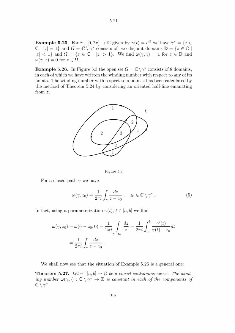
5.21

Example 5.25. For γ : [0, 2π]→ C given by γ(t) = eit we have γ∗ = z ∈C | |z| = 1 and G = C \ γ∗ consists of two disjoint domains D = z ∈ C ||z| < 1 and Ω = z ∈ C | |z| > 1. We find ω(γ, z) = 1 for z ∈ D andω(γ, z) = 0 for z ∈ Ω.

Example 5.26. In Figure 5.3 the open set G = C\γ∗ consists of 8 domains,in each of which we have written the winding number with respect to any of itspoints. The winding number with respect to a point z has been calculated bythe method of Theorem 5.24 by considering an oriented half-line emanatingfrom z.

1

1

1

2

2

2

3

0

Figure 5.3

For a closed path γ we have

ω(γ, z0) =1

2πi

∫

γ

dz

z − z0, z0 ∈ C \ γ∗ . (5)

In fact, using a parameterization γ(t), t ∈ [a, b] we find

ω(γ, z0) = ω(γ − z0, 0) =1

2πi

∫

γ−z0

dz

z=

1

2πi

∫ b

a

γ′(t)

γ(t)− z0dt

=1

2πi

∫

γ

dz

z − z0.

We shall now see that the situation of Example 5.26 is a general one:

Theorem 5.27. Let γ : [a, b]→ C be a closed continuous curve. The wind-ing number ω(γ, ·) : C \ γ∗ → Z is constant in each of the components ofC \ γ∗.

107

5.22

Proof. We only give the proof in the case where γ is a path, i.e. piecewiseC1. For z0 ∈ C \ γ∗ we choose r > 0 such that K(z0, 2r) ⊆ C \ γ∗. Forz1 ∈ K(z0, r) we have |z1 − γ(t)| ≥ r for each t ∈ [a, b], hence

ω(γ, z1)− ω(γ, z0) =1

2πi

∫

γ

(1

z − z1− 1

z − z0

)dz

=z1 − z02πi

∫

γ

dz

(z − z1)(z − z0).

By the estimation lemma 2.8 we get

|ω(γ, z1)− ω(γ, z0)| ≤|z1 − z0|2πr2

L(γ) ,

showing that ω(γ, ·) is continuous at the point z0.Let now G be a component of C \ γ∗. Using that G is path connected, we

infer from Theorem 5.7 that ω(γ, z) is constant for z ∈ G.

108

5.23

Exercises for §5

5.1. Let G ⊆ C be an open set and define a relation ∼ in G by

∀P,Q ∈ G : P ∼ Q ⇐⇒ P can be connected to Q by a staircase line

belonging to G

Prove that ∼ is an equivalence relation, i.e. has the properties

(i) P ∼ P (ii) P ∼ Q =⇒ Q ∼ P (iii) P ∼ Q ∧ Q ∼ R =⇒ P ∼ RFor P ∈ G define [P ] = Q ∈ G | P ∼ Q .

Prove that [P ] is a domain for every P ∈ G.Prove that if [P1] ∩ [P2] 6= ∅, then [P1] = [P2].

The sets [P ], P ∈ G are called the (connected) components of G. Giveexamples of open sets G ⊆ C, where the number of components is n =1, 2, . . . ,∞.

Prove that the number of components is countable.

5.2. Defining the sum of two sets A,B ⊆ C by

A+B = a+ b | a ∈ A , b ∈ B ,

prove that for z1, z2 ∈ C \ 0

arg(z1z2) = arg z1 + arg z2 ,

log(z1z2) = log z1 + log z2 .

Prove that if Re z1 > 0 and Re z2 > 0, then

Arg(z1z2) = Arg z1 +Arg z2 ,

Log (z1z2) = Log z1 + Log z2 ,

and show by examples that the two last equations do not hold for arbitraryz1, z2 ∈ C \ 0.

5.3. Prove that ln(x2 + y2) is harmonic in R2 \ (0, 0) and that Arctany

xis harmonic in (x, y) ∈ R2 | x > 0 .

5.4. Prove that the set T = z ∈ C | |z| = 1 does not have a continuousargument function.

109

5.24

Hint. Assume that θ : T → R is a continuous argument function withθ(1) = 0. Prove that Arg(z) = θ(z) for z ∈ T ∩ Cπ. Use this to determinethe limit of θ(z) for z = x+ iy ∈ T approaching −1 via y > 0 and via y < 0.

5.5. Let γ : [a, b] → C \ 0, δ : [b, c] → C \ 0 be continuous curves withγ(b) = δ(b), hence γ ∪ δ makes sense. Prove that

argvar (γ ∪ δ) = argvar (γ) + argvar (δ) .

5.6. Calculate Arg z and Log z for the following values of z ∈ C:

1 + i, −√3 + i , (

√3 + i)2001 .

5.7. Let γa : [0, 1] → C \ 0 be defined by γa(t) = eita, where a ∈ R.Determine argvar (γa). Prove that γa is closed if and only if a = 2πp, p ∈ Z,and prove that ω(γa, 0) = p when a = 2πp, p ∈ Z.

5.8. Let 0 < α < 1. Determine the image of the cut plane Cπ = C \ x ∈R | x ≤ 0 under the holomorphic branch of zα = exp(αLog z).

Prove that Arg(zα) = αArg(z), |zα| = |z|α for z ∈ Cπ.

5.9. Let G ⊆ C be open and assume that f ∈ H(G) is zero-free. Prove thatln |f | is a harmonic function in G.

5.10. Prove that cos√z can be considered as a well-defined function from C

to C. Prove that this function is holomorphic and determine its power serieswith centre 0.

5.11. For n ≥ 2, a ∈ C and α ∈ R we consider the half-lines

Lk =a+ rei(α+

k2πn

) | r ≥ 0, k = 0, 1, . . . , n− 1 ,

dividing C \ a in n angular domains

Vk =

z = a+ reiθ | r > 0 , α+ 2π

k − 1

n< θ < α+

2πk

n

,

k = 1, . . . , n. Make a sketch of these half-lines and angular domains. Provethat z 7→ (z − a)n maps each Vk bijectively onto Cnα and find the corre-sponding inverse function.

110

5.25

5.12. Let∑∞

n=0 anzn,∑∞

n=0 bnzn denote two power series, both assumed to

be absolutely convergent for |z| < ρ.1. Multiply the series by multiplying each term in one of the series

by each term in the other and collect the terms having the same factorzn, n = 0, 1, 2, . . . . Prove that this leads to the power series

a0b0 + (a0b1 + a1b0)z + (a0b2 + a1b1 + a2b0)z2 + · · · ,

or in more compact form

∞∑

n=0

cnzn, where cn =

n∑

k=0

akbn−k, n = 0, 1, . . . .

We call the power series∑∞

n=0 cnzn the Cauchy multiplication of the given

power series.

2. Prove that∑∞

n=0 cnzn is absolutely convergent for |z| < ρ and for

these z∞∑

n=0

cnzn = (

∞∑

n=0

anzn)(

∞∑

n=0

bnzn).

Hint to 2: Explain that the function f(z) = (∑∞

n=0 anzn)(∑∞

n=0 bnzn) is

holomorphic in K(0, ρ), and prove using exc. 1.16 that

f (n)(0)

n!=

n∑

k=0

akbn−k.

3. Using the Cauchy multiplication of two copies of the binomial series(α ∈ C)

(1 + z)α =

∞∑

n=0

(α

n

)zn, |z| < 1,

prove that (α+ β

n

)=

n∑

k=0

(α

k

)(β

n− k

),

where α, β ∈ C, n = 0, 1, . . . .

5.13. Let γ be a closed path in z ∈ C | |z| ≥ r. Prove that ω(γ, z) isconstant for z ∈ K(0, r).

5.14. Verify that the winding numbers are as indicated in Example 5.26.

111

5.26

5.15. Let G be an open path connected subset of C and let P ⊂ G bediscrete in G.

1. Let γ : [a, b]→ G be a continuous curve in G. Prove that γ∗ ∩ P is afinite set.

2. Let L be a staircase line in G with end points a, b ∈ G\P and assumethat the set L ∩ P , which is finite by 1, is written p1, . . . , pn. Prove thatthere exists a continuous curve from a to b in G\P consisting of line segmentsand circular arcs.

3. Conclude that G \ P is path connected.

5.16. Prove that

limn→∞

(1 +

z

n

)n= exp(z)

locally uniformly for z ∈ C by using Log . Compare with exc. 1.18.Hint. Fix a closed and bounded subset K in C. Prove that nLog (1+z/n)

is defined for z ∈ K if n is sufficiently big and converges to z uniformly onK.

112

6.1

§6. Zeros and isolated singularitiesA C∞-function on the real axis can be zero on an interval without being

identically zero. The following classical example is due to Cauchy

f(x) =

e−1/x , x > 0

0 , x ≤ 0 .

For holomorphic functions such a behaviour is not possible: Every zero a of aholomorphic function f is isolated in the sense that there are no other zerosin a sufficiently small disc K(a, r), unless of course f is identically zero. Thismakes it possible to prove an identity theorem for holomorphic functions: Iftwo holomorphic functions in a domain are equal on a tiny set (to be madeprecise), then they are identical. This result has far reaching consequences.

We will discuss isolated singularities for holomorphic functions and wewill classify them in one of three types: Removable singularities, poles andessential singularities. Around an isolated singularity a holomorphic functioncan be developed in a kind of power series which includes negative powers.It is called the Laurent series of the function. Quotients of holomorphicfunctions are called meromorphic. They have poles at points where thedenominator is zero. From an algebraic point of view we can consider theset M(G) of meromorphic functions as a field, namely the quotient field ofthe ring H(G) of holomorphic functions.

6.1. Zeros.

We recall that if a polynomial p of degree ≥ 1 has a zero (= root) a, i.e. ifp(a) = 0, then the polynomial can be factorized p(z) = (z − a)nq(z), whereq is a polynomial with q(a) 6= 0 and n ≥ 1 denotes the multiplicity or orderof the zero.

We shall extend this elementary result to holomorphic functions.

Theorem 6.1. Let f be holomorphic in a domain G and assume that f isnot identically 0. If a ∈ G is a zero of f , i.e. if f(a) = 0, then there existsa unique natural number n and a unique function g ∈ H(G) with g(a) 6= 0such that

f(z) = (z − a)ng(z) for z ∈ G . (1)

The number n is called the multiplicity or order of the zero.

Proof. We first prove the existence of the factorization (1).Let K(a, ρ) denote the biggest open disc centered at a and contained in

G. By Theorem 4.8 we have

f(z) =∞∑

k=0

f (k)(a)

k!(z − a)k , z ∈ K(a, ρ) . (2)

113

6.2

Assuming f (k)(a) = 0 for all k ≥ 0, we get f(z) = 0 for all z ∈ K(a, ρ),and we see below that f is identically zero in G in contradiction with theassumption.

Fix z0 ∈ G and choose a continuous curve γ : [0, 1]→ G connecting γ(0) =a with γ(1) = z0. By the paving lemma 5.2 there exist finitely many points0 = t0 < t1 < · · · < tn = 1 and a number r > 0 such that (1) and (2) fromthe paving lemma hold. In particular we have K(γ(0), r) = K(a, r) ⊆ G,hence K(a, r) ⊆ K(a, ρ). Moreover, γ(t1) ∈ K(a, r) and f is identically 0 inK(a, ρ), hence f (k)(γ(t1)) = 0 for all k ≥ 0. By Theorem 4.8 we get that fis identically 0 in K(γ(t1), r). In the same way we deduce successively thatf is identically 0 in all the discs K(γ(tk), r) and in particular that f(z0) = 0.

Having proved that our assumption leads to a contradiction, we see thatthere exists a smallest number n ≥ 1 such that f (n)(a) 6= 0, hence f (k)(a) = 0for k = 0, 1, . . . , n− 1. By equation (2) we then get

f(z) =∞∑

k=n

f (k)(a)

k!(z − a)k = (z − a)n

∞∑

k=0

f (k+n)(a)

(k + n)!(z − a)k (3)

for z ∈ K(a, ρ) ⊆ G. The function

g(z) =

f(z)(z−a)n for z ∈ G \ a,∑∞

k=0f (k+n)(a)(k+n)! (z − a)k for z ∈ K(a, ρ),

is well-defined on account of (3) and holomorphic in G. Moreover,

f(z) = (z − a)ng(z) for z ∈ G, g(a) = f (n)(a)/n! 6= 0 ,

which is a factorization of the type we want.To prove the uniqueness of the factorization (1), assume that

f(z) = (z − a)n1g1(z) = (z − a)n2g2(z) , z ∈ G (4)

where g1(a) 6= 0, g2(a) 6= 0. By reasons of symmetry we can assume thatn1 ≥ n2. By (4) we then get

(z − a)n1−n2g1(z) = g2(z) , z ∈ G \ a ,and by a continuity argument this equation also holds for z = a. Since weknow that g2(a) 6= 0 we get n1 = n2, hence g1(z) = g2(z) for all z ∈ G.

The theorem shows that the order of a zero a of f 6≡ 0 is the biggestnatural number n, for which there exists a factorization f(z) = (z − a)ng(z)with g ∈ H(G). If f(a) 6= 0, it is convenient to say that f has a zero of order0 in a. The order of the zero a of f is denoted ord(f, a). A zero of order 1 isalso called a simple zero, and a zero of order 2 is called a double zero.

From the proof of Theorem 6.1 we see the following:

114

6.3

Corollary 6.2. Let f be holomorphic in a domain G and assume that fis not identically 0. For a zero a ∈ G the order n is characterized by theequations

f(a) = f ′(a) = · · · = f (n−1)(a) = 0 , f (n)(a) 6= 0 .

Theorem 6.3. Let f be holomorphic in a domain G and assume that f isnot identically 0.

Every zero a of f is isolated in the sense that there exists r > 0 such thatf(z) 6= 0 for z ∈ K ′(a, r).

The set Z(f) of zeros of f is discrete in G and in particular Z(f) iscountable.

Proof. Let f(z) = (z−a)ng(z) be a factorization where g ∈ H(G) is such thatg(a) 6= 0. Since g is continuous, there exists ra > 0 such that |g(z)− g(a)| <|g(a)| for z ∈ K(a, ra) ⊆ G, hence g(z) 6= 0 for z ∈ K(a, ra). This showsthat f(z) 6= 0 for z ∈ K ′(a, ra).

We shall now prove that Z(f) has no accumulation points in G. We havejust proved that the points a ∈ Z(f) are not accumulation points of Z(f).

Assuming that z0 ∈ G \ Z(f) is an accumulation point of Z(f), thereexists a sequence of points (an) from Z(f) such that an → z0. By continuityof f we then get f(z0) = 0, contradicting z0 /∈ Z(f).

Having proved that the assumption was wrong, we know that Z(f) isdiscrete in G. By Theorem 5.6 it is countable.

The converse is also true: If P ⊆ G is an arbitrary discrete set in G, thenthere exists f ∈ H(G) such that Z(f) = P . It is even possible to assignmultiplicities np ∈ N to each p ∈ P and choose f such that ord(f, p) = np

for each p ∈ P . We skip the proof which depends on a general theory ofWeierstrass about factorization of entire functions. See Rudin’s book fordetails.

Example 6.4. The exponential function is zero-free in C. For the sinefunction we have Z(sin) = πZ, which is a countable discrete subset of C. Thefunction sin(1/z) is holomorphic in C \ 0 and has the zeros (pπ)−1 , p ∈Z \ 0, which have 0 as accumulation point. However, within C \ 0 thezero set has no accumulation points.

In analogy to the results about zeros of f ∈ H(G), let us fix λ ∈ C andconsider the set z ∈ G | f(z) = λ . This set is either equal to ∅ , G or acountable discrete subset of G. This is simply because the set in question isequal to Z(f − λ).

For these results it is important that G is path connected. If G = K(0, 1)∪K(2, 1), we can define f ∈ H(G) by setting f = 0 in one disc and f = 1 inthe other.

115

6.4

Theorem 6.5. (The identity theorem for holomorphic functions).If two holomorphic functions f, g in a domain G agree on a set A ⊆ G havingan accumulation point in G, then f(z) = g(z) for all z ∈ G.Proof. The zero set Z(f − g) is not discrete in G since it contains A, butthen f − g is identically zero in G.

A typical application of the theorem is the following: Assume that R∩G 6=∅ and that f(x) = g(x) for all x ∈ R ∩ G. Since R ∩ G contains a non-degenerate interval, it has accumulation points in G, hence f = g.

Example 6.6. As an application of the identity theorem it is possible toprove that all the usual trigonometric formulas known for real values of theargument also hold for complex values of the argument, provided the expres-sions are holomorphic.

As an example sin2 z + cos2 z = 1 for all z ∈ C. The expressions on theleft and right of the equality sign are holomorphic in C and agree for realnumbers.

Let f, g ∈ H(G) and assume that f(a) = g(a) = 0 for some a ∈ G. It isnot directly possible to determine

limz→a

f(z)

g(z),

because formally we get 0/0. L’Hospital’s rule from real analysis gets aparticularly simple form for holomorphic functions:

Theorem 6.7. (L’Hospital’s rule). Assume that f, g ∈ H(G) are notidentically zero in a disc around a ∈ G.

The limit

limz→a

f(z)

g(z)

exists if and only if ord(f, a) ≥ ord(g, a).If this condition is fulfilled, then

limz→a

f(z)

g(z)=f (q)(a)

g(q)(a),

where q = ord(g, a) and hence g(q)(a) 6= 0.

Proof. Let p = ord(f, a), q = ord(g, a) and let f1, g1 ∈ H(G) with f1(a) 6= 0,g1(a) 6= 0 such that

f(z) = (z − a)pf1(z) , g(z) = (z − a)qg1(z) .

116

6.5

If p ≥ q we find

limz→a

f(z)

g(z)= lim

z→a(z − a)p−q f1(z)

g1(z)=

0 , p > qf1(a)g1(a)

, p = q ,

but this expression is f (q)(a)/g(q)(a) because g(q)(a) = q!g1(a),

f (q)(a) =

0 , p > q

q!f1(a) , p = q .

If p < q we find

(z − a)q−p f(z)

g(z)=f1(z)

g1(z)−→ f1(a)

g1(a)6= 0 .

Therefore f(z)/g(z) can not have a limit for z → a. In fact, if the limitexisted then the left hand side would approach 0 for z → a because of thefactor (z − a)q−p.

6.2. Isolated singularities.

Definition 6.8. Let G ⊆ C be open and let a ∈ G. If f ∈ H(G \ a) wecall a an isolated singularity of f . If f can be given a complex value at asuch that f becomes differentiable at a (and hence holomorphic in G), thenthe singularity is said to be removable.

As an example where isolated singularities naturally appear, assume thatf ∈ H(G) is not identically zero in the domainG. The reciprocal function 1/fis holomorphic in G\Z(f), and all points a ∈ Z(f) are isolated singularities.The point 0 is an isolated singularity for 1/z, and the integers are isolatedsingularities for 1/ sin(πz).

In case of a being a removable singularity of f , the only possible value off at a making f differentiable at a is limz→a f(z), so a necessary conditionfor a to be removable is that the limit exists. That this condition is alsosufficient is not at all clear, but it will follow from the next theorem, becauseif f has a limit for z → a, then f is bounded in a sufficiently small punctureddisc K ′(a, r).

Theorem 6.9. Assume that f ∈ H(G \ a) is bounded in K ′(a, r) for anumber r > 0. Then f has a removable singularity at a.

Proof. We define h(a) = 0 and h(z) = (z − a)2f(z) for z ∈ G \ a. Then his clearly holomorphic in G \ a and for z 6= a we have

h(z) − h(a)z − a = (z − a)f(z) ,

117

6.6

which has the limit 0 for z → a because f is assumed to be bounded in apunctured disc around a.

This proves that h ∈ H(G) and h′(a) = 0. By Theorem 6.1 and Corollary6.2 there exists g ∈ H(G) such that h(z) = (z − a)2g(z) for z ∈ G. Thisshows that g(z) = f(z) for z ∈ G\ a and giving f the value g(a) for z = a,then f(= g) is differentiable at a, i.e. a is a removable singularity.

Notice that the boundedness condition of Theorem 6.9 implies the exis-tence of the limit limz→a f(z). This is quite remarkable.

The function sin z/z has a removable singularity for z = 0 because

limz→0

sin z

z= 1.

If f has an isolated singularity at z = a and the singularity is not re-movable, then the images f(K ′(a, r)) are unbounded sets regardless of howsmall r is. In particular f(z) does not have a limit for z → a. It is naturalto examine whether (z − a)mf(z) has a removable singularity for m ∈ N

sufficiently big. If this is the case a is called a pole.

Definition 6.10. An isolated singularity a is called a pole of order m ∈ N

of f , if (z − a)mf(z) has a limit for z → a and

limz→a

(z − a)mf(z) 6= 0 .

A pole of order 1 is called a simple pole.

The function f(z) = c/(z − a)m, where c 6= 0, m = 1, 2, . . . , has a pole oforder m for z = a. The expression (z − a)mf(z) is constant equal to c andhas in particular the limit c for z → a.

The order of a pole a is uniquely determined. In fact, if

limz→a

(z − a)mf(z) = c 6= 0,

then limz→a(z − a)kf(z) = 0 for k > m, while (z − a)kf(z) does not have alimit for z → a when k < m. Notice also that if a is a pole of order m ≥ 1,then |f(z)| → ∞ for z → a, because |z − a|m|f(z)| → |c|.

Assume that f ∈ H(G \ a) has a pole of order m at the point a. Thefunction

g(z) =

(z − a)mf(z) , z ∈ G \ a,limz→a(z − a)mf(z) , z = a,

is holomorphic in G, hence has a power series

g(z) =

∞∑

n=0

an(z − a)n

118

6.7

in the largest open disc K(a, ρ) ⊆ G. For z ∈ K ′(a, ρ) we then find

f(z) =a0

(z − a)m +a1

(z − a)m−1+ · · ·+ am−1

z − a +

∞∑

k=0

am+k(z − a)k . (1)

The function

p

(1

z − a

)=

m∑

k=1

am−k

(z − a)k , where p(z) =

m∑

k=1

am−kzk ,

is called the principal part of f at a.Subtracting the principal part from f gives us a holomorphic function

with a removable singularity at a. We can say that the singularity is “con-centrated” in the principal part.

An isolated singularity, which is neither removable nor a pole, is called anessential singularity. In a small punctured disc around such a singularity thebehaviour of f is very complicated as expressed byPicard’s great theorem:

For every r > 0 such that K(a, r) ⊆ G the image f(K ′(a, r)) is either C

or C with the exception of one point.We prove a weaker but still surprising result:

Theorem 6.11. (The Casorati-Weierstrass theorem). Suppose thatf ∈ H(G \ a) has an essential singularity at a. Then f(K ′(a, r)) is densein C9 for every r > 0 such that K(a, r) ⊆ G.Proof. Assuming the assertion not to be true, we can find r > 0 and a discK(c, ε) ⊆ C such that

K(c, ε) ∩ f(K ′(a, r)) = ∅,

hence |f(z) − c| ≥ ε for z ∈ K ′(a, r). Therefore g(z) = 1/(f(z) − c) isholomorphic in K ′(a, r) and bounded by 1/ε. By Theorem 6.9 we get thatg has a removable singularity at a. This makes it possible to assign a valueg(a) to g at a such that g becomes holomorphic in K(a, r). By definitiong(z) 6= 0 for z ∈ K ′(a, r).

If g(a) 6= 0 we have limz→a f(z) = c + 1/g(a) showing that f has aremovable singularity at a contrary to the hypothesis.

If g(a) = 0, then g has a zero at a, say of order m ≥ 1. By Theorem 6.1there exists g1 ∈ H(K(a, r)) such that

g(z) = (z − a)mg1(z) , g1(a) 6= 0 .

9A set A ⊆ C is called dense in C if A = C, i.e. if K(c, r) ∩A 6= ∅ for all c ∈ C, r > 0.

119

6.8

From the expression f(z) = c+ 1/g(z) we get

limz→a

(z − a)mf(z) = limz→a

((z − a)mc+ 1

g1(z)

)=

1

g1(a)6= 0 ,

which shows that f has a pole of order m at a, but also this contradicts thehypothesis.

6.3. Rational functions.

By a rational function of a complex variable we understand an expressionof the form p(z)/q(z), where p, q ∈ C[z], q 6= 0. Like ordinary fractions weconsider p1/q1 and p2/q2 as the same function if p1q2 = q1p2. If z = a is acommon zero of p and q, then (z−a) raised to a suitable power is a commondivisor of p and q, and it can be removed. In theoretical investigations wewill therefore always assume that the two polynomials p, q have no commonzeros. Under this assumption the function

f(z) =p(z)

q(z)

is holomorphic in C\Z(q) and Z(f) = Z(p). Let the zeros of q be a1, . . . , akwith the multiplicities m1, . . . , mk, hence

q(z) = c(z − a1)m1 · · · (z − ak)mk

for some constant c 6= 0, and it follows that a1, . . . , ak are isolated singu-larities of f and they are poles of multiplicities m1, . . . , mk. We have infact

(z − a1)m1f(z) =p(z)

c(z − a2)m2 · · · (z − ak)mk

−→ p(a1)

c(a1 − a2)m2 · · · (a1 − ak)mk6= 0

for z → a1, and similarly for a2, . . . , ak.The common notation in algebra of the set of rational functions is C(z).

This set is a field under addition and multiplication because every elementp/q from C(z) \ 0 has a reciprocal element q/p. It is the field of fractionsof the integral domain10 C[z].

10A commutative ring R is called an integral domain if for all a, b ∈ R, ab = 0 implies

a = 0 or b = 0.

120

6.9

Let us consider a rational function f = p/q, where deg(p) ≥ deg(q) and p, qhave no common zeros. Dividing p by q we get by Theorem 4.22 p = q1q+ rwith deg(r) < deg(q), hence

f(z) = q1(z) +r(z)

q(z).

We also see that r and q have no common zeros, because a common zero ofthese polynomials will also be a zero of p.

Theorem 6.12. (Partial fraction decomposition). Assume that r, q ∈C[z] have no common zeros and that 0 ≤ deg(r) < deg(q). Let a1, . . . , ak bethe zeros of q having the multiplicities m1, . . . , mk.

There exist uniquely determined constants cj,ℓ ∈ C such that

r(z)

q(z)=

k∑

j=1

mj∑

ℓ=1

cj,ℓ(z − aj)ℓ

. (1)

The formula (1) is called the partial fraction decomposition of the rationalfunction. The right-hand side is the sum of the principal parts of the function.

Proof. Uniqueness of the decomposition. Assume that we have a decomposi-tion (1). If r > 0 is so small that K(aj, r) does not contain any of the otherzeros of q, then (1) can be written

r(z)

q(z)= ϕ(z) +

mj∑

ℓ=1

cj,ℓ(z − aj)ℓ

,

where ϕ ∈ H(K(aj, r)). Multiplying this expression with (z − aj)mj , we get

r(z)

q(z)(z − aj)mj = ϕ(z)(z − aj)mj +

mj∑

ℓ=1

cj,ℓ(z − aj)mj−ℓ . (2)

The function (r(z)/q(z))(z− aj)mj has a removable singularity at z = aj , soin K(aj, r) it is the sum of its Taylor series with centre aj :

r(z)

q(z)(z − aj)mj =

∞∑

n=0

cn(z − aj)n . (3)

The coefficients cn in the Taylor series (3) are uniquely determined by theleft-hand side of (3). In fact n!cn is the n’th derivative of the left-hand sideof (3) at aj . Using that ϕ ∈ H(K(aj, r)), we see that ϕ(z)(z − aj)mj only

121

6.10

contributes to the Taylor series (3) with terms cn(z−aj)n for which n ≥ mj ,while the terms with n < mj come from the finite sum in (2), hence

cmj−ℓ = cj,ℓ , ℓ = 1, . . . , mj ,

showing that cj,ℓ is uniquely determined.

The existence of the decomposition.This is based on Liouville’s theorem. To each pole aj is associated a

principal partmj∑

ℓ=1

cj,ℓ(z − aj)ℓ

,

and if we subtract all the principal parts we get the function

f(z) =r(z)

q(z)−

k∑

j=1

mj∑

ℓ=1

cj,ℓ(z − aj)ℓ

,

which is holomorphic in C. Each of the terms

cj,ℓ(z − aj)ℓ

converge to 0 for |z| → ∞, and also the function r(z)/q(z) converges to 0 for|z| → ∞ because deg(q) > deg(r). This shows that f(z) → 0 for |z| → ∞,but then f is necessarily bounded and hence constant by Liouville’s theorem.A constant function approaching 0 for |z| → ∞ must be identically zero.

The coefficients in the representation (1) can be found using the uniquenessproof above. For every j we can calculate the first mj coefficients in theTaylor series for the function

r(z)

q(z)(z − aj)mj .

It is however easier to reduce the problem to solving a system of linearequations. The method is illustrated in the following example.

Example 6.13. The following partial fraction decomposition holds:

z3 + z2 − 6z + 3

z4 − 2z3 + z2=

1

z − 1− 1

(z − 1)2+

3

z2.

Factorizing z4 − 2z3 + z2 = z2(z − 1)2, we see that the fraction has poles oforder 2 at z = 0 and z = 1. Our goal is to determine the coefficients a, b, c, din the expression

z3 + z2 − 6z + 3

z2(z − 1)2=

a

z − 1+

b

(z − 1)2+c

z+

d

z2.

122

6.11

We know by Theorem 6.12 that such a decomposition is possible.Multiplying by z2(z − 1)2, we get

z3 + z2 − 6z + 3 = az2(z − 1) + bz2 + cz(z − 1)2 + d(z − 1)2

= (a+ c)z3 + (−a+ b− 2c+ d)z2 + (c− 2d)z + d ,

which is equivalent to the system of linear equations

a+ c = 1 , −a+ b− 2c+ d = 1 , c− 2d = −6 , d = 3 ,

having the solution: (a, b, c, d) = (1,−1, 0, 3).

Remark 6.14. The set C(z) is a vector space over the field C. The precedingtheory shows that the monomials 1, z, z2, . . . together with the functions1/(z − a)k, a ∈ C, k = 1, 2, . . . form a basis of the vector space.

6.4. Meromorphic functions.

A holomorphic function having only isolated singularities, which are ei-ther poles or removable singularities, is called a meromorphic function. It isnatural to assign ∞ as the value of the function at the poles, and thereforewe make the definition more precise in the following way:

Definition 6.15. A meromorphic function in a domain G ⊆ C is a mappingh : G→ C ∪ ∞ with the properties:

(i) P = z ∈ G | h(z) =∞ is discrete in G.(ii) The restriction f = h|G \ P is holomorphic in the open set G \ P .(iii) Every point a ∈ P is a pole of f .

Notice that the set of poles P of f is countable and G\P is open by Theorem5.6. The set of meromorphic11 functions in G is denotedM(G).

A holomorphic function in G is meromorphic with P = ∅.

We will now show how a quotient f/g of two holomorphic functions f, g ∈H(G) , g 6≡ 0, defines a meromorphic function h in G.

If f ≡ 0 we define h ≡ 0. Assume next that f 6≡ 0.Using that Z(g) is discrete in G, we see that h = f/g is holomorphic in

G \Z(g), and all points in Z(g) are isolated singularities of h. If a ∈ Z(g) isa zero of order q ≥ 1 of g, and a zero of order p ≥ 0 of f , then we can write

f(z) = (z − a)pf1(z) , g(z) = (z − a)qg1(z) ,11meromorphic is derived from Greek: fractional form in contrast to holomorphic:

whole form, “meros” meaning “part”, “holos” meaning “whole”.

123

6.12

where f1, g1 ∈ H(G) and f1(a), g1(a) are both different from zero. We there-fore see that

h(z) = (z − a)p−q f1(z)

g1(z),

for z ∈ K ′(a, r), where r is chosen so small that g1 is zero-free in K(a, r). Ifp ≥ q, then h has a removable singularity at a, and a is a zero of order p− q.If p < q, then h has a pole of order m = q− p at a, and we define h(a) =∞.This shows that h is a meromorphic function, and its set of poles consists ofthe points a ∈ Z(g) for which ord(g, a) > ord(f, a).

If h : G → C ∪ ∞ is meromorphic and a ∈ G is a pole of order m,then f(z) = (z − a)mh(z) is holomorphic in a suitable disc K(a, r), henceh(z) = f(z)/(z−a)m in K ′(a, r). This shows that a meromorphic function his locally a quotient of holomorphic functions, but this actually holds globally:

There exist f, g ∈ H(G) where g 6≡ 0 such that h = f/g.

If P is the set of poles of h, there exists by §6.1 a holomorphic functiong ∈ H(G) such that Z(g) = P , and g can be chosen such that the order ofevery zero a ∈ Z(g) is equal to the order of the pole a of h. The function hgis holomorphic in G \ P , but having removable singularities at the points ofP . There exists thus f ∈ H(G), such that f = hg in G \ P , hence h = f/g.

We can add and multiply two meromorphic functions h1, h2 : G→ C∪∞by performing the addition and multiplication outside the union of the twosets of poles, giving a holomorphic function there. All the points in the unionof the two sets of poles are isolated singularities which are either removableor poles, hence defining a meromorphic function. If h is meromorphic andnot the zero function, then the reciprocal function 1/h is also meromorphic.Zeros of h of order n are poles of 1/h of order n, and poles of h of orderm are zeros of 1/h of order m. It is easy to verify that the set M(G) ofmeromorphic functions in a domain G is a field. The representation h = f/gof an arbitrary meromorphic function as a quotient of holomorphic functionsshows that the field of meromorphic functions is isomorphic to the field offractions of the integral domain H(G), cf. exc. 6.2.

A rational function is meromorphic in C having only finitely many poles.

6.5. Laurent series.

The function exp( 1z ) is holomorphic in C \ 0 and z = 0 is an isolated

124

6.13

singularity. We know from real analysis that for all n ≥ 0

limx→0+

xn exp

(1

x

)= lim

y→∞exp(y)

yn=∞ ,

limx→0−

xn exp

(1

x

)= lim

y→∞(−1)n exp(−y)

yn= 0 ,

hence zn exp( 1z ) has no limit for z → 0, showing that z = 0 is neither aremovable singularity nor a pole. Therefore z = 0 is an essential singularity.

Inserting the power series for exp we get

exp

(1

z

)=

∞∑

n=0

1

n!zn, z ∈ C \ 0 .

We shall study a type of infinite series generalizing power series and in-cluding the series above for exp

(1z

).

Definition 6.16. A Laurent series12 is a doubly infinite series of the form

∞∑

n=−∞cnz

n , (1)

where (cn)n∈Z are given complex numbers and z ∈ C \ 0.

Concerning convergence of a Laurent series (1), we shall consider it as sumof two ordinary infinite series

∞∑

n=1

c−nz−n +

∞∑

n=0

cnzn ,

and we require each of them to be convergent. These series are power seriesin the variable 1/z and z respectively. Denoting their radii of convergenceρ1, ρ2 respectively, we see that the first series is absolutely convergent for|1/z| < ρ1, the second for |z| < ρ2. Only the case 1/ρ1 < ρ2 is interesting,for then the series (1) is absolutely convergent in the annulus

G = z ∈ C | 1/ρ1 < |z| < ρ2,

which is the domain between the two concentric circles centered at 0 withradii 1/ρ1, ρ2. (If 1/ρ1 ≥ ρ2 then G = ∅). In case ρ1 = ∞ we have G =K ′(0, ρ2) if ρ2 <∞, and G = C \ 0 if ρ2 =∞.

12Named after the French engineer P.A. Laurent (1813-1854).

125

6.14

The Laurent series converges locally uniformly in the annulus to thesum function, showing that it is holomorphic by Corollary 4.19. In fact,by Theorem 4.5 both power series converge uniformly on sets of the formr1 ≤ |z| ≤ r2, where 1/ρ1 < r1 ≤ r2 < ρ2, and since an arbitrary compactsubset K of G is contained in z ∈ C | r1 ≤ |z| ≤ r2 for suitable r1, r2 suchthat 1/ρ1 < r1 ≤ r2 < ρ2, the assertion follows. As suitable numbers we cansimply use r1 = inf|z| | z ∈ K, r2 = sup|z| | z ∈ K.

Generalizing the above, we call the infinite series

∞∑

n=−∞cn(z − a)n

a Laurent series with centre a ∈ C. It represents a holomorphic function inan annulus with centre a:

A(a;R1, R2) = z ∈ C | R1 < |z − a| < R2 ,

where 0 ≤ R1 < R2 ≤ ∞ is the inner and outer radius respectively.Laurent proved the converse of this, namely that every holomorphic func-

tion in an annulus is the sum function of a suitable Laurent series:

Theorem 6.17. Assume that f is holomorphic in the annulus A(a;R1, R2).Then f is the sum of a uniquely determined Laurent series

f(z) =∞∑

n=−∞cn(z − a)n for z ∈ A(a;R1, R2), (2)

and the coefficients of the series are given by

cn =1

2πi

∫

∂K(a,r)

f(z)

(z − a)n+1dz , n ∈ Z , (3)

independent of r ∈ ]R1, R2[.

Proof. We first show that if a Laurent series (2) is convergent with sum f(z)for z ∈ A(a, R1, R2), then the coefficients are given by (3), hence uniquelydetermined by f . In fact, using that the series (2) is uniformly convergentfor z ∈ ∂K(a, r), we get by Theorem 4.6 (ii) that

1

2πi

∫

∂K(a,r)

f(z)

(z − a)n+1dz =

1

2πi

∫

∂K(a,r)

( ∞∑

k=−∞ck(z − a)k−n−1

)dz =

∞∑

k=−∞ck

1

2πi

∫

∂K(a,r)

(z − a)k−n−1dz = cn1

2πi

∫

∂K(a,r)

dz

z − a = cn .

126

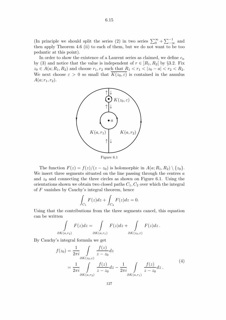
6.15

(In principle we should split the series (2) in two series∑∞

0 +∑−1

−∞ andthen apply Theorem 4.6 (ii) to each of them, but we do not want to be toopedantic at this point).

In order to show the existence of a Laurent series as claimed, we define cnby (3) and notice that the value is independent of r ∈ ]R1, R2[ by §3.2. Fixz0 ∈ A(a;R1, R2) and choose r1, r2 such that R1 < r1 < |z0 − a| < r2 < R2.

We next choose ε > 0 so small that K(z0, ε) is contained in the annulusA(a; r1, r2).

•

•

K(a, r1) K(a, r2)

K(z0, ε)

a

↓

↓

↓

↑

↑

↑

Figure 6.1

The function F (z) = f(z)/(z − z0) is holomorphic in A(a;R1, R2) \ z0.We insert three segments situated on the line passing through the centres aand z0 and connecting the three circles as shown on Figure 6.1. Using theorientations shown we obtain two closed paths C1, C2 over which the integralof F vanishes by Cauchy’s integral theorem, hence

∫

C1

F (z)dz +

∫

C2

F (z)dz = 0.

Using that the contributions from the three segments cancel, this equationcan be written∫

∂K(a,r2)

F (z)dz =

∫

∂K(a,r1)

F (z)dz +

∫

∂K(z0,ε)

F (z)dz .

By Cauchy’s integral formula we get

f(z0) =1

2πi

∫

∂K(z0,ε)

f(z)

z − z0dz

=1

2πi

∫

∂K(a,r2)

f(z)

z − z0dz − 1

2πi

∫

∂K(a,r1)

f(z)

z − z0dz .

(4)

127

6.16

We now transform the first integral into an infinite series in analogy withTheorem 4.8.

For z ∈ ∂K(a, r2) we have

1

z − z0=

1

z − a1

1− z0−az−a

,

where |(z0 − a)/(z − a)| = |z0−a|r2

< 1. The last fraction is the sum of aninfinite geometric series giving

1

z − z0=

1

z − a

∞∑

n=0

(z0 − az − a

)n

,

hencef(z)

z − z0=

∞∑

n=0

f(z)

(z − a)n+1(z0 − a)n . (5)

This series being uniformly convergent for z ∈ ∂K(a, r2), we are allowed tointegrate term by term in (5), hence

1

2πi

∫

∂K(a,r2)

f(z)

z − z0dz =

∞∑

n=0

1

2πi

∫

∂K(a,r2)

f(z)

(z − a)n+1dz

(z0 − a)n

=∞∑

n=0

cn(z0 − a)n .

The series being convergent for arbitrary z0 in the annulus, we see that itsradius of convergence is ≥ R2.

For z ∈ ∂K(a, r1) we have similarly

1

z − z0=

1

a− z01

1− z−az0−a

,

where |(z − a)/(z0 − a)| = r1|z0−a| < 1, showing that the last fraction is the

sum of an infinite geometric series, hence

1

z − z0=

1

a− z0

∞∑

n=0

(z − az0 − a

)n

giving

f(z)

z − z0= −

∞∑

n=0

f(z)

(z0 − a)n+1(z − a)n . (6)

128

6.17

The series being uniformly convergent for z ∈ ∂K(a, r1), we can integrateterm by term in (6) to get

1

2πi

∫

∂K(a,r1)

f(z)

z − z0dz = −

∞∑

n=0

1

2πi

∫

∂K(a,r1)

f(z)(z − a)ndz

(z0 − a)−n−1 ,

= −∞∑

n=0

c−n−1(z0 − a)−n−1 .

The series being convergent for arbitrary z0 in the annulus and being a powerseries in the variable 1/(z0 − a), we see that the series converges for any z0such that |z0 − a| > R1, hence the power series

∞∑

n=1

c−nwn

has a radius of convergence ≥ 1/R1.By (4) we now get

f(z0) =

∞∑

n=0

cn(z0 − a)n +

∞∑

n=1

c−n

(z0 − a)n=

∞∑

−∞cn(z0 − a)n .

Remark 6.18. To a holomorphic function f in the annulus A(a;R1, R2) isassociated a holomorphic function fi in K(a, R2) with the power series

fi(z) =

∞∑

n=0

cn(z − a)n

and a holomorphic function fe in z ∈ C | |z − a| > R1 with the seriesexpansion

fe(z) =

∞∑

n=1

c−n

(z − a)n .

For z ∈ A(a;R1, R2) we have

f(z) = fi(z) + fe(z) .4

4The indices i and e are chosen for interior and exterior.

129

6.18

Remark 6.19. Let f be holomorphic in the annulus A(a;R1, R2).For r ∈ ]R1, R2[ we consider the function

gr(θ) = f(a+ reiθ) , θ ∈ R

which is periodic with period 2π. By (2) we get

gr(θ) =

∞∑

n=−∞cnr

neinθ ,

and this series converges uniformly for θ ∈ R, and is thus the Fourier series ofgr. Inserting the parameterization a+ reiθ of ∂K(a, r), we can write formula(3) as

cnrn =

1

2π

∫ 2π

0

gr(θ)e−inθdθ ,

which is the usual formula for the Fourier coefficients.

Let G ⊆ C be open and let a ∈ G. If f ∈ H(G \ a), then f has anisolated singularity at a. Let K(a, ρ) denote the largest open disc centeredat a and contained in G. In particular, f is holomorphic in the annulusK ′(a, ρ) = A(a; 0, ρ), hence possesses a Laurent series

f(z) =

∞∑

n=−∞cn(z − a)n , z ∈ K ′(a, ρ) (7)

with

cn =1

2πi

∫

∂K(a,r)

f(z)

(z − a)n+1dz , n ∈ Z , (8)

where r ∈ ]0, ρ[ is arbitrary.By the Remark 6.18 we get a holomorphic function fi ∈ H(K(a, ρ)) given

by

fi(z) =

∞∑

n=0

cn(z − a)n ,

and a holomorphic function fe ∈ H(C \ a) given by

fe(z) =

∞∑

n=1

c−n

(z − a)n (9)

associated with the Laurent series, and we have

f(z) = fi(z) + fe(z) for z ∈ K ′(a, ρ) . (10)

130

6.19

Definition 6.20. Let f ∈ H(G \ a). The function fe(z) given by (9) iscalled the principal part of f .

By (10) we see that f(z)−fe(z), which is holomorphic in G\a, has a re-movable singularity at z = a and fi(z) determines the holomorphic extensionto the point a, the value at a being fi(a) = c0.

We shall now see how the type of the isolated singularity can be determinedfrom the coefficients cn of the Laurent series with negative index n.

Theorem 6.21. The isolated singularity a of f ∈ H(G \ a) with Laurentseries (7) is

(i) removable, if and only if cn = 0 for n < 0,(ii) a pole, if and only if cn = 0 for all n < 0 except finitely many. The

order of the pole is the biggest m > 0 such that c−m 6= 0,(iii) an essential singularity, if and only if cn 6= 0 for infinitely many

n < 0.

Proof. (i) If cn = 0 for n < 0, then fe = 0 and fi determines the holomorphicextension of f to a with the value f(a) = c0 = fi(a). Assume next that a isa removable singularity. Then the limit

c := limz→a

f(z)

exists and in particular there exists r0 > 0 (r0 < ρ) such that

|f(z)− c| ≤ 1 for z ∈ K ′(a, r0) . (11)

Based on (11) we shall show that cn = 0 when n < 0.By (8) we have for 0 < r < ρ

cn =1

2πi

∫

∂K(a,r)

f(z)(z − a)−n−1dz ,

but since n < 0 we have −n − 1 ≥ 0, hence (z − a)−n−1 has a primitive(z − a)−n/(−n). This gives

∫

∂K(a,r)

(z − a)−n−1dz = 0 ,

and hence

cn =1

2πi

∫

∂K(a,r)

(f(z)− c)(z − a)−n−1dz .

131

6.20

By the estimation lemma 2.8 and (11) we get for r < r0

|cn| ≤2πr

2π· 1 · r−n−1 = r−n,

and remembering that −n > 0, we get cn = 0 by letting r → 0.

(ii) If c−m 6= 0 for an m ≥ 1 and c−n = 0 for n > m, then we can rewrite(7):

f(z) =c−m

(z − a)m +c−(m−1)

(z − a)m−1+ · · ·+ c−1

z − a +

∞∑

n=0

cn(z − a)n,

hence

(z − a)mf(z) =m−1∑

k=0

c−m+k(z − a)k + (z − a)m∞∑

n=0

cn(z − a)n ,

showing thatlimz→a

(z − a)mf(z) = c−m 6= 0 ,

i.e. a is a pole of order m.If conversely z = a is a pole of order m ≥ 1, then the function (z−a)mf(z)

has a removable singularity. The Laurent series of (z − a)mf(z) is obtainedby multiplying (7) with (z − a)m, hence

(z − a)mf(z) =∞∑

n=−∞cn(z − a)n+m =

∞∑

k=−∞ck−m(z − a)k .

By case (i) we infer that ck−m = 0 for k < 0, hence cn = 0 for n < −m.

(iii) The assertion is a consequence of (i) and (ii), because an essentialsingularity is an isolated singularity, which is neither removable nor a pole.Similarly, the condition for cn in (iii) is precisely excluding the conditions forcn in (i) and (ii).

Example 6.22. Let f : C → C be an entire transcendental function, i.e.an entire function which is not a polynomial. Equivalently, infinitely manycoefficients cn in the power series

f(z) =∞∑

n=0

cnzn , z ∈ C

are different from 0.

132

6.21

The function f(1z

), z ∈ C \ 0 has an isolated singularity at z = 0 and

we have the series expansion

f

(1

z

)=

∞∑

n=0

cnzn

, z ∈ C \ 0 . (12)

Because of the uniqueness of a Laurent series, we see that (12) is the Laurentseries of f

(1z

). Having assumed that cn 6= 0 for infinitely many n, we see

that z = 0 is an essential singularity.

Example 6.23. The function

f(z) =1

z − 2− 1

z − 1=

1

z2 − 3z + 2

is holomorphic in C \ 1, 2, and in particular it is holomorphic in K(0, 1)and in the annuli A(0; 1, 2) and A(0; 2,∞).

We shall determine the corresponding series expansions.In K(0, 1) f(z) has a power series:

f(z) =1

1− z −1

2

1

1− z2

=

∞∑

n=0

(1− 1

2n+1

)zn .

For 1 < |z| < 2 we can make the following calculation

f(z) = −1

z

1

1− 1z

− 1

2

1

1− z2

= −∞∑

n=1

1

zn−

∞∑

n=0

1

2n+1zn ,

which is the Laurent series in A(0; 1, 2). For 2 < |z| we find

f(z) = −1

z

1

1− 1z

+1

z

1

1− 2z

= −∞∑

n=1

1

zn+

∞∑

n=1

2n−1

zn

=∞∑

n=2

(2n−1 − 1

) 1

zn.

We get three different series expansions in three disjoint domains. It is im-portant not to mix up these series, but there are four more series of interest,two Laurent series with centre 1 and two Laurent series with centre 2.

The function has a simple pole at z = 1. It therefore has a Laurent serieswith centre 1 in the annulus A(1; 0, 1), i.e. for z verifying 0 < |z − 1| < 1:

f(z) = − 1

1− (z − 1)− 1

z − 1= − 1

z − 1−

∞∑

n=0

(z − 1)n .

133

6.22

It has another Laurent series in the annulus A(1; 1,∞), i.e. valid for |z−1| >1:

f(z) =1

(z − 1)(1− 1z−1 )

− 1

z − 1=

∞∑

n=2

1

(z − 1)n.

The function has also a simple pole at z = 2. It is holomorphic in theannulus A(2; 0, 1) and has therefore a Laurent series with centre z = 2 validfor 0 < |z − 2| < 1:

f(z) =1

z − 2− 1

1 + (z − 2)=

1

z − 2+

∞∑

n=0

(−1)n+1(z − 2)n .

In the annulus A(2; 1,∞), i.e. for |z − 2| > 1 we have

f(z) =1

z − 2− 1

(z − 2)(1 + 1z−2 )

=

∞∑

n=2

(−1)n(z − 2)n

.

Remark about the radius of convergence. Let f ∈ H(C \ P ), whereP ⊆ C is discrete in C, and assume that none of the singularities a ∈ P areremovable. For every z0 ∈ C \ P we can represent f by a power series

f(z) =

∞∑

n=0

an(z − z0)n (13)

in the largest open disc K(z0, ρ) ⊆ C \ P . It is clear that

ρ = inf|z0 − a| | a ∈ P .

Notice that the infimum is actually a minimum, hence ρ = |z0 − a| for somepoint a ∈ P , cf. Lemma A.1 with K = z0, F = P .

Theorem 6.24. With the notation above the radius of convergence of (13)is equal to ρ.

Proof. By Theorem 4.8 we know that the radius of convergence R satisfiesR ≥ ρ. Assuming R > ρ, we see that (13) defines a holomorphic extensionof f to K(z0, R). However, a point a ∈ P satisfying |a − z0| = ρ belongsto K(z0, R), but then a has to be a removable singularity, contradicting theassumption.

134

6.23

Exercises for §6

6.1. Let G be a domain in C and assume that f ∈ H(G) has only finitelymany zeros in G. Prove that there exists a polynomial p(z) and a zero-freefunction ϕ ∈ H(G) such that f(z) = p(z)ϕ(z) for z ∈ G.

6.2. Let G ⊆ C be open. Prove that the ring H(G) is an integral domain ifand only if G is path connected.

Recall that a commutative ring R is an integral domain if

∀a, b ∈ R : ab = 0⇒ a = 0 ∨ b = 0.

6.3. The reflection principle. The mapping z → z is a reflection in the realaxis.

1 Let G ⊆ C be open and f ∈ H(G). The reflected set and the reflectedfunction are defined by

G∗ = z ∈ C | z ∈ G f∗ : G∗ → C , f∗(z) = f(z) , z ∈ G∗ .

Prove that f∗ ∈ H(G∗) and that (f∗)′ = (f ′)∗.

2 Let G ⊆ C be a domain which is reflection invariant, i.e. G = G∗.Prove that G ∩ R 6= ∅.

Prove that f ∈ H(G) is real-valued on G ∩ R if and only if f is reflectioninvariant, i.e. f = f∗ or

f(z) = f(z) for all z ∈ G .

Hint. Make use of the identity theorem.

3 Prove that an entire function f(z) =∑∞

0 anzn is reflection invariant if

and only if an ∈ R for n = 0, 1, . . . .

6.4. Determine a ∈ C such that sin z − z(1 + az2) cos z has a zero of fifthorder at z = 0.

6.5. Assume that h : C→ C∪∞ is meromorphic with finitely many polesz1, . . . , zn and assume that there exist k > 0 , N ∈ N and R > 0 such that|h(z)| ≤ k|z|N for |z| > R. Prove that h is a rational function.

Hint. Make use of exc. 4.9.

135

6.24

6.6. Prove that

4z3

(z2 + 1)2=

2

z + i− i

(z + i)2+

2

z − i +i

(z − i)2 .

6.7. Find the partial fraction decomposition of the rational function

f(z) =2z − (2 + i)

z2 − (2 + i)z + 2i

and find next its Laurent series in the annulus A(0; 1, 2).

6.8. Let f be holomorphic in the annulus A(a;R1, R2) and let fi, fe be theholomorphic functions from Remark 6.18. Prove that

fe(z)→ 0 for |z − a| → ∞ .

Assume next that there exists a holomorphic function φi in K(a, R2) anda holomorphic function φe in the domain z ∈ C | |z − a| > R1 such that

φe(z)→ 0 for |z − a| → ∞ ,

andf(z) = φi(z) + φe(z) for z ∈ A(a;R1, R2) .

Prove that fi(z) = φi(z) for z ∈ K(a, R2) and fe(z) = φe(z) for |z−a| > R1.Hint. Make use of Liouville’s Theorem for the function

g(z) =

fi(z) − φi(z) , |z − a| < R2

φe(z) − fe(z) , |z − a| > R1 .

6.9. Let f ∈ H(G), where G is a simply connected domain. Let γ be a closedpath in G. Prove the following extension of Cauchy’s integral formula

ω(γ, z0)f(z0) =1

2πi

∫

γ

f(z)

z − z0dz , z0 ∈ G \ γ∗ .

Hint. Make use of the fact that z 7→ (f(z)−f(z0))/(z−z0) has a removablesingularity at z0.

6.10. Let a ∈ C. Determine the Laurent series in the annulus (puncturedplane) C \ a of the function

f(z) =exp(z)

(z − a)3 .

136

6.25

6.11. For z ∈ C we consider the function

f(ω) = exp

(z

2

(ω − 1

ω

)), ω ∈ C \ 0 ,

which is holomorphic in C\0. Prove that the Laurent series can be written

exp

(z

2

(ω − 1

ω

))=

∞∑

n=−∞Jn(z)ω

n , ω ∈ C \ 0 ,

where

Jn(z) =1

2π

π∫

−π

ei(z sin t−nt)dt =1

π

∫ π

0

cos(z sin t− nt)dt , n ∈ Z .

The function Jn : C→ C is called the Bessel function of order n.Prove that

z(Jn−1(z) + Jn+1(z)) = 2nJn(z) .

6.12. Explain why f(z) = z/(ez − 1) has a removable singularity at z = 0and is holomorphic in the disc K(0, 2π). The power series of f with centrez = 0 is denoted

z

ez − 1=

∞∑

n=0

Bn

n!zn , hence Bn = f (n)(0) .

Prove that the radius of convergence is 2π and that the Bernoulli numbersBn are determined by the equations

B0 = 1 ,

n∑

k=0

Bk

(n+ 1

k

)= 0 , n = 1, 2, . . . .

Prove that each Bn is a rational number and verify the values

B1 = −1

2, B2 =

1

6, B3 = 0 , B4 = − 1

30.

Prove that the function

g(z) =z

ez − 1− 1 +

z

2

is even (i.e. g(−z) = g(z)) and conclude that B2n+1 = 0 for n ≥ 1.

137

6.26

6.13. Prove that the Laurent series of cot z, 0 < |z| < π, is given by

cot z =1

z+

∞∑

k=1

(−1)k B2k

(2k)!22kz2k−1 ,

where Bn are the Bernoulli numbers from exc. 6.12.Hint. Make use of Euler’s formulas from Theorem 1.16.

6.14. Let z1, . . . , zn ∈ K(0, r) be mutually different, let α1, . . . , αn ∈ C andconsider the rational function

f(z) =

n∑

j=1

αj

z − zj,

which is holomorphic C \ z1, . . . , zn.Prove that f has a primitive in the domain z ∈ C | |z| > r if and only

ifn∑

j=1

αj = 0.

Hint. Make use of Theorem 2.13 and exc. 5.13.

6.15. Prove that the function z/(1− z − z2) has simple poles at z = (−1 ±√5)/2 and determine the radius of convergence of the power series:

z

1− z − z2 =

∞∑

0

Fnzn .

Prove that F0 = 0, F1 = 1, Fn = Fn−1 + Fn−2, n ≥ 2. (This is the sequenceof Fibonacci numbers: 0, 1, 1, 2, 3, 5, 8, . . .).

Find the partial fraction decomposition of the rational function and useit to prove Binet’s formula

Fn =1√5

[(1 +√5

2

)n

−(1−√5

2

)n].

6.16. Prove that Picard’s Theorem 4.21 can be deduced from Picard’s greattheorem on p. 6.7.

Hint. Let f be an entire function. Look at f(1/z) in C \ 0.

138

7.1

§7. The calculus of residues

In this section we introduce residues and prove Cauchy’s residue theorem,which can be seen as the culmination of the complex analysis developed byCauchy. In addition to theoretical applications like the theorem of Rouche,the residue theorem makes it possible to calculate definite integrals and toevaluate sums of infinite series.

The fact that an integral of the type∫ ∞

−∞

x2

(x2 + 1)2dx

can be evaluated by calculating a residue at z = i can seem like magic.

7.1. The residue theorem.

Let f ∈ H(G \ a) have an isolated singularity at z = a ∈ G and let

f(z) =

∞∑

n=−∞cn(z − a)n (1)

be the Laurent series with centre a.The coefficient c−1 is particularly important and is called the residue of f

at the point a. It is denoted Res(f, a), hence by §6.5 (8)

Res(f, a) = c−1 =1

2πi

∫

∂K(a,r)

f(z)dz (2)

for 0 < r < ρ, where K(a, ρ) is the largest open disc in G centered at a.Residues were introduced by Cauchy. The residue is what remains, apart

from the factor 2πi, when the function f is integrated along a path sur-rounding the singularity. By §3.2 the circle ∂K(a, r) can be replaced byother simple closed paths moving counterclockwise around the singularity.

We shall now formulate and prove Cauchy’s residue theorem. Because ofits many applications, it is one of the most important theorems in complexanalysis. We note that it includes the integral theorem and the integralformula of Cauchy.

Theorem 7.1. (Cauchy’s residue theorem). Let G be a simply con-nected domain and let P = a1, . . . , an ⊆ G. Let γ be a simple closed pathin G surrounding a1, . . . , an with positive orientation.13 For f ∈ H(G \ P )we have ∫

γ

f(z)dz = 2πin∑

j=1

Res(f, aj) .

13We use an intuitive geometric formulation.

139

7.2

Proof. Let pj denote the principal part of f at the point aj , j = 1, . . . , n, cf.Definition 6.20. Then ϕ = f − (p1 + · · ·+ pn) has a removable singularity ateach of the points a1, . . . , an, and therefore it has a holomorphic extensionto G. By Cauchy’s integral theorem we know that

∫γϕ = 0, hence

∫

γ

f =

n∑

j=1

∫

γ

pj .

The principal part pj is holomorphic in C \ aj. For r > 0 sufficiently small

the path γ also surrounds K(aj , r) and using the idea of §3.2 it can be provedthat ∫

γ

pj =

∫

∂K(aj ,r)

pj .

(We skip the details. In concrete applications of the theorem these mattersare usually obvious). Assume that the principal part pj is given by theexpansion

pj(z) =

∞∑

n=1

cj,n(z − aj)n

.

The series being uniformly convergent on ∂K(aj, r), we see by Theorem 4.6(ii) that

∫

∂K(aj ,r)

pj =

∞∑

n=1

∫

∂K(aj ,r)

cj,n(z − aj)n

dz = 2πiRes(f, aj).

In fact, only the term for n = 1 yields a contribution, namely 2πi Res(f, aj),because the integrands in the terms for higher values of n have a primitive.

We shall now give some simple devices for calculating residues at poles ofa meromorphic function h.

1 Assume that h has a simple pole at a.Then

Res(h, a) = limz→a

(z − a)h(z) .

In fact, in a sufficiently small disc K(a, r) we have by the Laurent expansion

h(z) =Res(h, a)

z − a + ϕ(z) ,

and ϕ is holomorphic.

140

7.3

2 Assume that h = f/g, where f, g are holomorphic such that f(a) 6= 0,g(a) = 0 , g′(a) 6= 0, hence h has a simple pole at a.

ThenRes(h, a) = f(a)/g′(a) .

In fact, by 1 we get

Res(h, a) = limz→a

f(z)z − ag(z)

= limz→a

f(z)

(g(z)− g(a)z − a

)−1

=f(a)

g′(a).

3 Assume that h has a pole of order m ≥ 1 at a.Defining ϕ(z) = (z − a)mh(z), then ϕ has a removable singularity at a

and we get

Res(h, a) =ϕ(m−1)(a)

(m− 1)!.

In fact, by the Laurent expansion of h similar to (1) we get

ϕ(z) = c−m + c−m+1(z − a) + · · ·+ c−1(z − a)m−1 + c0(z − a)m + · · · (3)

and we know c−1 = Res(h, a). However, the coefficient c−1 to (z − a)m−1 in(3) can also be found as the right-hand side of the formula we want to prove.

Example 7.2. (i) The residue of the rational function z 7→ 1/(1+z2) at z =±i is ∓ i

2. This follows by 2, but can also be inferred from the decomposition

1

1 + z2=

i

2(z + i)− i

2(z − i) .

(ii) The meromorphic function z 7→ 1/ sin z has a simple pole at z = nπ ,n ∈ Z. The residue at z = nπ is 1/ cos(nπ) = (−1)n by 2.

(iii) The function

h(z) =z sin z

1− cos z

is meromorphic in C. The zeros of the denominator are 2pπ , p ∈ Z, andthey all have multiplicity 2. The numerator has a double zero at z = 0 andsimple zeros at z = pπ , p ∈ Z \ 0. We conclude that z = 0 is a removablesingularity and z = 2pπ , p ∈ Z \ 0 are simple poles of h.

To find the value of h at the removable singularity z = 0, we develop thenumerator and the denominator in power series using the known power seriesfor sin and cos:

h(z) =z(z − z3

3! +− · · ·)

z2

2! − z4

4! +− · · ·=

1− z2

3! +− · · ·12! − z2

4! +− · · ·→ 2 for z → 0 .

141

7.4

Alternatively we can make use of L’Hospital’s rule (Theorem 6.7), yielding

limz→0

h(z) =f (2)(0)

g(2)(0)= 2,

where f(z) = z sin z, g(z) = 1− cos z.To calculate the residues at 2pπ , p 6= 0 we put w = z − 2pπ, and by the

periodicity of sin and cos we get

(z − 2pπ)h(z) =w(w + 2pπ) sin(w + 2pπ)

1− cos(w + 2pπ)

=(w + 2pπ)w sinw

1− cosw= (w + 2pπ)h(w).

Moreover, since z → 2pπ ⇔ w → 0 we find

Res(h, 2pπ) = limz→2pπ

(z − 2pπ)h(z) = limw→0

(w + 2pπ)h(w) = 4pπ.

Here we also used limw→0 h(w) = 2 as shown above.

(iv) h(z) = z2(z2 +1)−2 is a rational function with poles of order 2 at thepoints z = ±i. We find the residues using 3. Defining

ϕ(z) = (z − i)2h(z) = z2

(z + i)2,

we get

ϕ′(z) =2iz

(z + i)3,

hence Res(h, i) = ϕ′(i) = − i4 . Analogously we get Res(h,−i) = i

4 .

7.2. The principle of argument.

The residue theorem can be used to calculate the number of zeros andpoles of a meromorphic function.

Theorem 7.3. Let h : G→ C∪∞ be meromorphic in a simply connecteddomain G and let γ be a positively oriented simple closed path in G notpassing through any zeros or poles of h. Then

1

2πi

∫

γ

h′(z)

h(z)dz = Z − P,

142

7.5

where Z is the number of zeros and P the number of poles of h in the sub-domain of G enclosed by γ. In the calculation of Z and P a zero or a poleof order m is counted as m.

Proof. Let D be the set of zeros or poles of h. Then h′/h is holomorphic inG \D. We will see that h′/h is meromorphic having D as the set of poles.Letting a denote a zero of h of order n, we have for z ∈ K(a, r), where r issufficiently small,

h(z) = an(z − a)n + an+1(z − a)n+1 + · · · , an 6= 0 ,

henceh′(z) = n an(z − a)n−1 + (n+ 1)an+1(z − a)n + · · · ,

leading to

h′(z)

h(z)=

n

z − a1 + (n+1)an+1

nan(z − a) + · · ·

1 + an+1

an(z − a) + · · · ,

which proves that h′/h has a simple pole at a with the residue n. Letting bdenote a pole of h of order m, we have for z ∈ K ′(b, r), where r is sufficientlysmall,

h(z) = c−m(z − b)−m + c−(m−1)(z − b)−(m−1) + · · · , c−m 6= 0 ,

hence

h′(z) = −m c−m(z − b)−(m+1) − (m− 1)c−(m−1)(z − b)−m − · · · ,

leading to

h′(z)

h(z)=−mz − b

1 +(m−1)c

−(m−1)

mc−m(z − b) + · · ·

1 +c−(m−1)

c−m(z − b) + · · · ,

which proves that h′/h has a simple pole at b with the residue −m.Let a1, . . . , an be those points from D which are enclosed by γ. We

now use an intuitive fact (which we do not prove) that there exists a simplyconnected sub-domain G1 ⊆ G such that D ∩ G1 = a1, . . . , an. Applyingthe residue theorem for h′/h ∈ H(G1 \ a1, . . . , an), we get

1

2πi

∫

γ

h′(z)

h(z)dz =

n∑

j=1

Res(h′/h, aj) = Z − P,

since Res(h′/h, aj) = ±m with + if aj is a zero and − if aj is a pole of orderm.

143

7.6

Remark 7.4. (The principle of argument). Let Γ = h γ be the closedpath obtained by taking the values of h along γ. Notice that Γ stays inC \ 0, because h has no zeros and poles on γ∗. Denoting the interval ofdefinition of γ by [a, b], then the integral from Theorem 7.3 is equal to

1

2πi

∫ b

a

h′(γ(t))γ′(t)

h(γ(t))dt =

1

2πi

∫

Γ

dz

z= ω(Γ, 0) .

We can thus express the result of Theorem 7.3 as

ω(Γ, 0) = Z − P

orargvar (Γ) = 2π(Z − P ) .

This is the reason for calling Theorem 7.3 the principle of argument: Acontinuous branch of arg(h(γ(t))) changes its value by 2π(Z−P ) by followingthe path once in positive orientation.

As an example let us consider h(z) = sin z for z ∈ C. If we followsin z along the unit circle counterclockwise, then a continuous branch ofarg(sin(eit)) will increase by 2π because sin z has a simple zero z = 0 in-side the unit circle. Furthermore, if we follow sin2 z around the circle |z| = 4,the argument will increase by 12π because there are 3 double zeros in thedisc K(0, 4).

Theorem 7.5. (Rouche’s Theorem)14. Let f, g ∈ H(G) in a simplyconnected domain G. Let γ be a simple closed path in G such that

|f(z)− g(z)| < |f(z)|+ |g(z)| for z ∈ γ∗ . (1)

Then f and g have the same number of zeros counted with multiplicity in thebounded domain enclosed by γ.

Proof. By (1) we get that f(z) 6= 0 and g(z) 6= 0 for z ∈ γ∗. The functionF (z) = g(z)/f(z) is meromorphic in G and

F ′

F=g′

g− f ′

f.

The setG = z ∈ G | f(z) 6= 0

is open and γ∗ ⊆ G ⊆ G, F ∈ H(G). The assumption (1) about f, g can beexpressed

|1− F (z)| < 1 + |F (z)| for z ∈ γ∗,14Eugene Rouche, French mathematician, 1832-1910.

144

7.7

and F being continuous in G, we get that

Ω := z ∈ G | |1− F (z)| < 1 + |F (z)|

is open and γ∗ ⊆ Ω. Note that w ∈ C | |1 − w| < 1 + |w| = Cπ, soF (Ω) ⊆ Cπ.

Since Log is holomorphic in Cπ, we see that Log F is holomorphic in Ωand is a primitive of F ′/F in Ω, hence

0 =1

2πi

∫

γ

F ′

F=

1

2πi

∫

γ

g′

g− 1

2πi

∫

γ

f ′

f.

If γ is positively oriented, then the assertion follows by Theorem 7.3.

As an application of Rouche’s theorem we will give a proof of the funda-mental theorem of algebra, cf. Theorem 4.23.

Let g(z) = zn + an−1zn−1 + · · · + a1z + a0 be a normalized polynomial

of degree n ≥ 1 and let f(z) = zn. On the circle γ(t) = Reit, t ∈ [0, 2π] wehave |f(z)| = Rn and

|f(z)− g(z)| ≤ |an−1|Rn−1 + · · ·+ |a1|R + |a0|.

The right-hand side of the inequality is < Rn provided R is sufficiently big,i.e. provided R ≥ R0 for suitable R0. This shows that f and g have thesame number of zeros in the disc K(0, R0). Clearly, f(z) = zn has z = 0 as azero of multiplicity n, and therefore g has n zeros in K(0, R0) counted withmultiplicity.

As another application of Rouche’s theorem we shall prove the open map-ping theorem:

Theorem 7.6. Let f be a non-constant holomorphic function in a domainG ⊆ C. Then f(G) is a domain in C.

In particular f is an open mapping, i.e. f(Ω) is open in C for every opensubset Ω ⊆ G.Proof. The second part follows from the first part because every open setΩ ⊆ G is a union of discs

Ω =⋃

i∈I

K(ai, ri) ,

and thereforef(Ω) =

⋃

i∈I

f(K(ai, ri))

145

7.8

is the union of the domains f(K(ai, ri)), hence open.We shall now prove that f(G) is open, hence a domain, the latter because

of Theorem A.6, which implies that f(G) is path connected since G is so.Fix w0 = f(z0) for z0 ∈ G. We shall find ρ > 0 such that K(w0, ρ) ⊆

f(G). To do this we consider the function ϕ(z) = f(z) − w0, which hasa zero at z = z0, and let k ≥ 1 be the order of this zero. Since zeros ofholomorphic functions are isolated, there exists r > 0 such that K(z0, r) ⊆ Gand f(z)− w0 6= 0 for z ∈ K(z0, r) \ z0.

By Theorem A.3 we thus get

ρ := inf|f(z)− w0| | z ∈ ∂K(z0, r) > 0.

By Lemma 3.6 there exists R > 0 such that K(z0, r) ⊂ K(z0, R) ⊂ G.Fixing w ∈ K(w0, ρ), we will apply Rouche’s Theorem to the two functions

ϕ(z) = f(z)−w0, ψ(z) = f(z)−w, which are both holomorphic in G, hencein K(z0, R).

For |z − z0| = r we have

|ϕ(z)− ψ(z)| = |w − w0| < ρ ≤ |ϕ(z)|,

and therefore ψ has the same number of zeros in K(z0, r) as ϕ has, namelyk zeros, i.e. there exist z ∈ K(z0, r) such that ψ(z) = f(z)− w = 0.

Summing up: To every w ∈ K(w0, ρ) there exists z ∈ K(z0, r) such thatf(z) = w, hence K(w0, ρ) ⊆ f(K(z0, r)) ⊆ f(G).

7.3. Calculation of definite integrals.

The residue theorem can be applied to calculate definite integrals. An ideato calculate

∫∞−∞ f(x)dx is roughly speaking this: Choose a closed path γ in

C containing the segment [−R,R], e.g. a half-circle over the segment or arectangle having the segment as one side. Consider a meromorphic functionF in C agreeing with f on the real axis (often it suffices just to write f(z)instead of f(x)). The integral of f from −R to R plus the integral alongthe remaining part of the path is equal to 2πi multiplied by the sum of theresidues at the poles inside the path. Letting R→∞, it often happens thatthe contribution from “the remaining part of the path” tends to 0, and inthe limit we find the integral in question.

Example 7.7. Let us calculate

∫ ∞

−∞

x2

(x2 + 1)2dx .

146

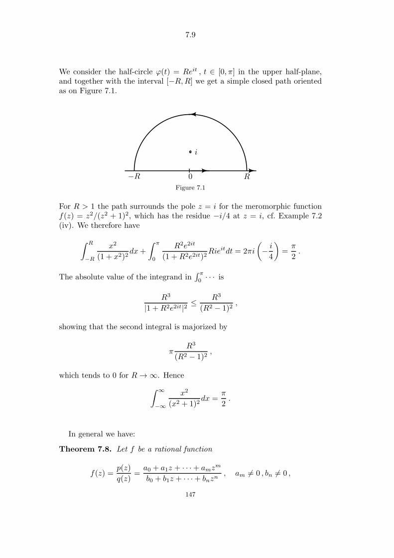
7.9

We consider the half-circle ϕ(t) = Reit , t ∈ [0, π] in the upper half-plane,and together with the interval [−R,R] we get a simple closed path orientedas on Figure 7.1.

i

−R 0 R

Figure 7.1

For R > 1 the path surrounds the pole z = i for the meromorphic functionf(z) = z2/(z2 + 1)2, which has the residue −i/4 at z = i, cf. Example 7.2(iv). We therefore have

∫ R

−R

x2

(1 + x2)2dx+

∫ π

0

R2e2it

(1 +R2e2it)2Rieitdt = 2πi

(− i4

)=π

2.

The absolute value of the integrand in∫ π

0· · · is

R3

|1 +R2e2it|2 ≤R3

(R2 − 1)2,

showing that the second integral is majorized by

πR3

(R2 − 1)2,

which tends to 0 for R→∞. Hence

∫ ∞

−∞

x2

(x2 + 1)2dx =

π

2.

In general we have:

Theorem 7.8. Let f be a rational function

f(z) =p(z)

q(z)=a0 + a1z + · · ·+ amz

m

b0 + b1z + · · ·+ bnzn, am 6= 0 , bn 6= 0 ,

147

7.10

and assume that n ≥ m+ 2 and that f has no poles on the real axis. Then

∫ ∞

−∞f(x)dx = 2πi

k∑

j=1

Res(f, zj) ,

where z1, . . . , zk are the poles in the upper half-plane.

Proof. Since

lim|z|→∞

zn−mf(z) =ambn

there exists R0 > 0 such that

|z|n−m|f(z)| ≤M :=|am||bn|

+ 1 for |z| ≥ R0 ,

or

|f(z)| ≤ M

|z|2 for |z| ≥ max(1, R0) .

Choosing R > 0 bigger than max(1, R0) and so big that K(0, R) contains allpoles of f in the upper half-plane, we have

∫ R

−R

f(x) dx+

∫ π

0

f(Reiθ)iReiθ dθ = 2πi

k∑

j=1

Res(f, zj) .

The absolute value of the second integral is majorized by π R(M/R2), which

tends to 0 for R → ∞, and therefore the integral∫ R

−Rf(x) dx tends to the

right-hand side, which is independent of R.

Remark 7.9. If w1, . . . , wl denote the poles of f in the lower half-plane,then analogously

∫ ∞

−∞f(x) dx = −2πi

l∑

j=1

Res(f, wj) .

The method of Theorem 7.8 can be applied to other meromorphic func-tions than rational, provided that the integral over the half-circle tends to 0for R→∞.

The following theorem can be used to calculate integrals for the form∫ ∞

−∞f(x)eiλx dx,

which are called Fourier integrals.

148

7.11

Theorem 7.10. Let f be meromorphic in C without poles on the real axisand with only finitely many poles z1, . . . , zk in the upper half-plane. If

max0≤t≤π

|f(Reit)| → 0 for R→∞,

then

limR→∞

∫ R

−R

f(x)eiλxdx = 2πik∑

j=1

Res(f(z)eiλz, zj) for λ > 0 .

Proof. We consider the simple closed path consisting of the segment [−R,R]and the half-circle |z| = R , Im z ≥ 0 oriented counterclockwise, and we con-sider only R so big that the path encloses all the poles z1, . . . , zk. ApplyingCauchy’s residue theorem to f(z)eiλz, we find

∫ R

−R

f(x)eiλxdx+

∫ π

0

f(Reit)eiλReitiReitdt = 2πik∑

j=1

Res(f(z)eiλz , zj

).

The absolute value of the second integral is majorized by

I = max0≤t≤π

|f(Reit)|∫ π

0

Re−λR sin t dt ,

but using sin t ≥ 2π t for t ∈ [0, π2 ], see the Figure 7.2,

(π2 , 1)

Figure 7.2

we get15 with a = 2λR/π:

∫ π

0

e−λR sin tdt = 2

∫ π/2

0

e−λR sin tdt ≤ 2

∫ π/2

0

e−atdt

=2

a

(1− e−aπ

2

)<

2

a=

π

λR,

henceI ≤ π

λmax0≤t≤π

|f(Reit)| ,

which tends to 0 for R→∞, and the theorem is proved.

15The integral is split in integrals over [0, π/2] and [π/2, π], and the last integral is

transformed using sin t = sin(π − t).

149

7.12

Remark 7.11. If w1, . . . , wl denote the poles of f in the lower half-plane,and the half-circle lies there, then we have to assume that

maxπ≤t≤2π

|f(Reit)| → 0 for R→∞,

and we get in an analogous way that

limR→∞

∫ R

−R

f(x)eiλxdx = −2πil∑

j=1

Res(f(z)eiλz, wj) for λ < 0 .

Example 7.12. We shall prove that

limR→∞

∫ R

−R

x sinλx

x2 + 1dx = π e−λ for λ > 0 .

The function f(z) = z/(z2 + 1) is meromorphic with the poles z = ±i and

Res(f(z)eiλz , i) = 12e

−λ.

The inequality

max0≤t≤π

|f(Reit)| ≤ R

R2 − 1for R > 1

shows that the conditions of Theorem 7.10 are satisfied, hence

limR→∞

∫ R

−R

x eiλx

x2 + 1dx = πi e−λ for λ > 0 ,

and taking the imaginary part, we get the result. (Taking the real part leadsto

limR→∞

∫ R

−R

x cos(λx)

x2 + 1dx = 0,

which is obvious.)

Example 7.13. We shall prove that

limR→∞

∫ R

−R

sinx

xdx = π .

Define f(z) = eiz/z. Then f has a simple pole at z = 0 with the residue 1.We next integrate f along the positively oriented path of Figure 7.3, and

the result is 2πi by the residue theorem. The small half-circle with theparameterization

cr(t) = r eit , t ∈ [−π, 0]

150

7.13

contributes with the amount

∫

cr

eiz

zdz =

∫

cr

dz

z+

∫

cr

eiz − 1

zdz = iπ + α(r) ,

but since

ϕ(z) =eiz − 1

z→ i for z → 0,

(e.g. by l’Hospital’s rule), there exists r0 > 0 such that |ϕ(z)| ≤ 2 for |z| ≤ r0,hence |α(r)| ≤ 2πr for r ≤ r0. This shows that limr→0 α(r) = 0, hence

limr→0

∫

cr

eiz

zdz = iπ .

−R + iR R + iRI2

I3 I1

−R −r r R

Figure 7.3

The integral I1 along the vertical side z = R + it , t ∈ [0, R] is

I1 =

∫ R

0

eiR−t

R + iti dt,

hence

|I1| ≤∫ R

0

e−t

Rdt ≤ 1

R

∫ ∞

0

e−tdt =1

R→ 0 for R→∞ .

The integral I2 along the upper side z = −t+ iR , t ∈ [−R,R] is

I2 = −∫ R

−R

e−it−R

−t+ iRdt,

hence

|I2| ≤ e−R

∫ R

−R

dt

R= 2e−R → 0 for R→∞ .

151

7.14

The integral I3 along the vertical side z = −R + i(R− t) , t ∈ [0, R] is

I3 = −i∫ R

0

e−iR+t−R

−R + i(R − t)dt,

hence

|I3| ≤1

R

∫ R

0

et−Rdt ≤ 1

R→ 0 for R→∞ .

Using that

I1 + I2 + I3 +

∫ −r

−R

+

∫ R

r

eix

xdx+ iπ + α(r) = 2πi ,

we get by taking the imaginary part and letting r → 0

Im (I1 + I2 + I3) +

∫ R

−R

sinx

xdx+ π = 2π.

Finally, by letting R→∞, we get (remembering Ij → 0 for j = 1, 2, 3)

limR→∞

∫ R

−R

sinx

xdx = π,

hence ∫ ∞

−∞

sinx

xdx = π ,

∫ ∞

0

sinx

xdx =

π

2.

We notice that the integrals are improper in the sense that the integral ofthe absolute value diverges:∫ ∞

−∞

∣∣∣sinx

x

∣∣∣dx =∞ .

The latter follows by comparison with the harmonic series because

∫ ∞

0

| sinx|x

dx ≥n∑

k=1

kπ∫

(k−1)π

| sinx|x

dx ≥n∑

k=1

1

kπ

kπ∫

(k−1)π

| sinx|dx

=2

π

n∑

k=1

1

k.

To evaluate an integral of the form∫ 2π

0

f(cos t, sin t)dt,

one can try to rewrite it as a path integral over the unit circle∫

∂K(0,1)

f

(1

2(z +

1

z) ,

1

2i(z − 1

z)

)1

izdz

using that z = eit , t ∈ [0, 2π] is a parameterization. We next try to evaluatethis integral by the residue theorem.

152

7.15

Example 7.14. Evaluate

I(a) =

∫ 2π

0

dt

a+ cos tfor a > 1 .

We find

I(a) =

∫

∂K(0,1)

dz

iz(a + 12 (z +

1z ))

= −2i∫

∂K(0,1)

dz

z2 + 2az + 1.

The polynomial in the denominator has the zeros p = −a +√a2 − 1 , q =

−a−√a2 − 1 , hence q < −1 < p < 0. The integrand has a simple pole z = p

in K(0, 1) with the residue[

1

2z + 2a

]

z=p

=1

2√a2 − 1

,

while q /∈ K(0, 1). By the residue theorem

I(a) = (−2i)(2πi) 1

2√a2 − 1

=2π√a2 − 1

.

7.4. Sums of infinite series.

Let f be meromorphic in C. The meromorphic functions

f(z) cot(πz), f(z)/ sin(πz)

have isolated singularities at z = n ∈ Z with

Res(f(z) cot(πz), n) =f(n)

π

Res(f(z)/ sin(πz), n) =(−1)nf(n)

π,

provided that f does not have a pole at z = n.If f(n) = 0, then z = n is in fact a removable singularity and the residue

is 0. If z = n is a pole of f , then we have to modify the expression for theresidue, since the pole becomes multiple.

Let γm,n denote a simple closed path surrounding the poles −m,−m +1, . . . , 0, 1, . . . , n counterclockwise, where m,n ∈ N0. For f ∈ H(C) we have

∫

γm,n

f(z) cot(πz)dz = 2in∑

k=−m

f(k) (1)

∫

γm,n

f(z)

sin(πz)dz = 2i

n∑

k=−m

(−1)kf(k) . (2)

153

7.16

If we can find the limit of the left-hand sides form,n→∞, we get expressionsfor the sums

∞∑

−∞f(k) ,

∞∑

−∞(−1)kf(k) .

If we can find the limits when m = 0 and for n → ∞, we similarly getexpressions for the sums

∞∑

0

f(k) ,∞∑

0

(−1)kf(k) .

If f has poles, then the right-hand sides of (1) and (2) have to be modified.

As a closed path we choose the boundary of the rectangle

Fm,n = z = x+ iy | −(m+

1

2

)≤ x ≤ n+

1

2, |y| ≤ n+m , n,m ≥ 1 .

Using

sin(πz) = sin(πx) cosh(πy) + i cos(πx) sinh(πy),

cf. exc. 1.12, we get the following estimates on the vertical sides of Fm,n

| sin(πz)| = cosh(πy) =1

2

(eπy + e−πy

)≥ 1

2eπ|y|,

hence1

| sin(πz)| ≤ 2e−π|y| ≤ 2 . (3)

On the horizontal sides y = ± (n+m) of Fm,n we have

| sin(πz)|2 = sin2(πx) cosh2(πy) + cos2(πx) sinh2(πy)

= sin2(πx)(1 + sinh2(πy)) + cos2(πx) sinh2(πy)

= sin2(πx) + sinh2(πy)

≥ sinh2(πy) = sinh2(π(n+m)),

hence1

| sin(πz)| ≤1

sinh(π(n+m))≤ 1

sinh(2π). (4)

154

7.17

Example 7.15. Let f(z) = 1/z2. The function 1/(z2 sin(πz)) has a pole ofthird order at z = 0 with the residue π/6 (see below), while z = k ∈ Z \ 0is a simple pole with the residue (−1)k/(πk2). By the residue theorem wethen get ∫

∂Fm,n

dz

z2 sin(πz)= 2πi

π

6+ 2i

n∑

k=−mk 6=0

(−1)kk2

. (5)

Since (−1)k/k2 has the same value for ± k, k ∈ N, it is convenient to putm = n. The length of the rectangle Fn,n is

L(∂Fn,n) = 2(2n+ 1) + 8n = 12n+ 2 ,

and for z ∈ ∂Fn,n we have |z| > n.From (3) and (4) we see that

1

| sin(πz)| ≤ 2 for z ∈ ∂Fn,n ,

hence by the estimation lemma 2.8

∣∣∣∫

∂Fn,n

dz

z2 sin(πz)

∣∣∣ ≤ 2

n2(12n+ 2)→ 0 for n→∞ ,

and we finally get by (5) that

∞∑

k=1

(−1)k−1

k2=π2

12. (6)

Evaluation of the residue Res(1/(z2 sin(πz)), 0).We calculate the first terms of the power series of z/ sin z. Using that it

is an even function with the value 1 at the removable singularity z = 0, wecan write

z

sin z= 1 + k1z

2 + k2z4 + · · · .

Multiplying this power series by the well-known power series

sin z

z= 1− z2

6+z4

5!−+ · · ·

we get

1 = 1 +

(k1 −

1

6

)z2 +

(k2 −

k16

+1

5!

)z4 + · · · ,

hence k1 − 16 = 0, k2 − k1

6 + 15! = 0, . . . , leading to k1 = 1

6 , k2 = 7360 .

155

7.18

This gives

1

z2 sin(πz)=

1

πz3

(1 +

π2

6z2 + k2π

4z4 + · · ·),

from where we can read off that the residue is π6.

As the last application of the residue theorem we will prove Euler’s partialfraction decomposition of 1/ sin z.

Theorem 7.16. For z ∈ C \ πZ

1

sin z=

∞∑

p=−∞

(−1)pz − pπ =

1

z+ 2z

∞∑

p=1

(−1)pz2 − p2π2

.

More precisely we have

n∑

p=−m

(−1)pz − pπ →

1

sin zfor n,m→∞,

uniformly for z in every bounded subset of C \ πZ.

Proof. Fix a ∈ C \ Z and consider f(z) = 1/(z − a). Then1

(z − a) sin(πz) ,

has simple poles at z = a and z = k ∈ Z, the residues being

1

sin(πa)and

(−1)kπ(k − a) .

Integrating along the boundary of the rectangle Fm,n above, moving coun-terclockwise, where m,n ∈ N are chosen so big that a is an interior point ofFm,n, we get

I =1

2πi

∫

∂Fm,n

dz

(z − a) sin(πz) =1

sin(πa)−

n∑

k=−m

(−1)kπ(a− k) .

We shall prove that I → 0 for n,m → ∞, uniformly for a belonging to abounded subset of C \ Z.

By (3) and (4) we get

|I| ≤ 1

2πsup

1

|z − a|∣∣ z ∈ ∂Fm,n

(4

n+m∫

−(n+m)

e−π|y|dy + 2n+m+ 1

sinhπ(n+m)

),

156

7.19

and since

4

n+m∫

−(n+m)

e−π|y|dy = 8

n+m∫

0

e−πydy ≤ 8

πand sup

x+ 1

sinh(πx)| x ≥ 2

<∞,

there exists a constant K, independent of n and m, such that

|I| ≤ K sup 1

|z − a|∣∣ z ∈ ∂Fm,n

.

Assume now that a ∈ K(0, R) \ Z, where R is fixed and consider m,n > R.For z ∈ ∂Fm,n we have |z − a| > min(m,n)−R, hence

|I| < K

min(m,n)−R → 0

uniformly for a ∈ K(0, R) \ Z when m,n→∞. This shows what we wantedto prove, hence

1

sin(πa)=

∞∑

k=−∞

(−1)kπ(a− k) .

Replacing a by zπ we get the original formula.

157

7.20

Exercises for §7

7.1. Find the poles, their order and the corresponding residues of

f(z) =1

z(z − 1)2, f(z) =

1

z(z + 1)3, f(z) =

1

ez2 − 1.

7.2. (This exercise requires exc. 6.3.) Let h : C→ C∪∞ be a meromorphicfunction with P being the set of poles.

1 Prove that the reflected function h∗ : C→ C ∪ ∞ defined by

h∗(z) =

h(z), for z /∈ P ∗

∞, for z ∈ P ∗

is a meromorphic function with the set of poles P ∗ = p|p ∈ P.2 If a is a pole of order m of h with the principal part

m∑

j=1

cj(z − a)j ,

then a is a pole of h∗ of the same order and with the principal part

m∑

j=1

cj(z − a)j ,

and in particular Res(h∗, a) = Res(h, a) for a ∈ P .3 Prove that C\ (P ∪P ∗) is a reflection invariant domain. Hint. Use exc.

5.15.

4 Prove that h(R \ P ) ⊆ R if and only if P = P ∗ and h = h∗.

7.3. Let f, g ∈ H(G) and assume that f has a zero of order n > 0 at a ∈ Gand that g has a zero of order n+ 1 at a. Prove that

Res

(f

g, a

)= (n+ 1)

f (n)(a)

g(n+1)(a).

7.4. Let h : G→ C ∪ ∞ be meromorphic in the simply connected domainG, let ϕ ∈ H(G) and let γ be a positively oriented simple closed path in G,not passing through any zeros and poles of h. Assume that γ encloses the

158

7.21

zeros a1, . . . , ap and the poles b1, . . . , bq of h, each of them repeated as oftenas the multiplicity indicates.

Prove that

1

2πi

∫

γ

h′(z)

h(z)ϕ(z)dz =

p∑

j=1

ϕ(aj)−q∑

j=1

ϕ(bj) .

7.5. Prove that

1

2πi

∫

∂K(0,n+ 12 )

z2k cot(πz)dz =2

π

n∑

j=1

j2k.

for n, k ∈ N.

7.6. Prove that

∫ ∞

−∞

dx

1 + x4=

π√2,

∫ ∞

0

xdx

1 + x4=π

4.

7.7. Prove that

∫ ∞

−∞

x2

(x2 + 1)(x2 + 4)dx =

π

3.

7.8. Prove that

∫ ∞

−∞

eiπx

x2 − 2x+ 2dx = −πe−π .

7.9. Prove that

∫ 2π

0

cosx

a+ cosxdx = 2π

(1− a√

a2 − 1

)for a > 1.

7.10. Prove that

∫ ∞

0

xp−1

1 + x2ndx =

π

2n sin pπ2n

, p, n ∈ N, 1 ≤ p < 2n.

Hint. Integrate along the boundary of the sector z = |z|eiθ , |z| ≤ R , 0 ≤θ ≤ π

n ).

7.11. Prove that

∫ ∞

−∞

eax

1 + exdx =

π

sin(aπ)for 0 < a < 1 .

159

7.22

Hint. Integrate along the boundary of the rectangle with vertices z =±R , z = ±R + 2πi.

7.12. Prove that∫ ∞

0

x4n+3e−x sinx dx = 0 for n = 0, 1, 2, . . . .

Hint. Integrate f(z) = z4n+3e−z along the boundary of the sector z = |z|eiθ,0 ≤ |z| ≤ R , 0 ≤ θ ≤ π

4 .Prove that

∫ ∞

0

tne−4√t sin

4√t dt = 0 , n = 0, 1, 2, . . . .

For every c ∈ [−1, 1] consider the measure µc on [0,∞[ having the non-

negative density (1+c sin 4√t)e−

4√t with respect to Lebesgue measure. Provethat all the measures µc have the same moments

∫ ∞

0

xn dµc(x) = 4(4n+ 3)!.

(This is the example of Stieltjes of an indeterminate moment problem, i.e.that different measures on [0,∞[ can have the same moments.)

7.13. Prove that∫ ∞

−∞

eiλx

1 + x2dx = πe−|λ| , λ ∈ R .

7.14. Prove that

| cot z|2 =cos2 x+ sinh2 y

sin2 x+ sinh2 yfor z = x+ iy ∈ C \ πZ

and use it to conclude that | cot(πz)| < 2 for z ∈ ∂Fn,n in the notation from§7.4.

Prove that

∞∑

k=1

1

k2p= −π

2Res

(cot(πz)

z2p, 0

)p ∈ N .

Calculate the residue using exc. 6.13 and prove Euler’s formula

∞∑

k=1

1

k2p= (−1)p−1 B2p

2(2p)!(2π)2p .

160

7.23

7.15. Let f ∈ H(G) be non-constant in the domain G. Fix z0 ∈ G and let

f(z0) = w0. Prove that there exists r > 0 with K(z0, r) ⊆ G and such that

(i) f(z) 6= w0 for z ∈ K(z0, r) \ z0.(ii) f ′(z) 6= 0 for z ∈ K(z0, r) \ z0.

Assume that the zero z0 of f(z)− w0 has order k ≥ 2.Recall the proof of Theorem 7.6 and define Γ(t) = f(z0 + reit), t ∈ [0, 2π]

and ρ > 0 such that K(w0, ρ) ∩ Γ∗ = ∅.Prove that for every w ∈ K(w0, ρ) the function f(z) − w has k simple

zeros in K(z0, r).Explain that the following theorem has been proved:Let f ∈ H(G) be one-to-one (injective) on the domain G. Then f ′(z) 6= 0

for all z ∈ G.Comment. By Theorem 7.6 we know that f(G) is open and f : G→ f(G) isan open mapping. Use this to prove that f−1 is continuous and prove nextthat it is also holomorphic, hence Theorem 1.4 has been proved, when G isa domain.

7.16. Let f be holomorphic in the domain G. Fix z0 ∈ G, let f(z0) = w0

and assume that f ′(z0) 6= 0.Prove that there exist an open set U such that z0 ∈ U ⊆ G and a ρ > 0

such that f maps U bijectively onto K(w0, ρ).Hint. Make use of the proof of Theorem 7.6.

7.17. Let f be a non-constant holomorphic function in the domain G. Fixz0 ∈ G, let f(z0) = w0 and assume that f ′(z0) = · · · = f (k−1)(z0) = 0,f (k)(z0) 6= 0 for some k ≥ 1. Prove that there exist an open set U suchthat z0 ∈ U ⊆ G and a holomorphic function h : U → C satisfying h(z0) =0, h′(z0) 6= 0 such that

f(z) = w0 + (h(z))k for z ∈ U .

Hint. Make use of the Taylor expansion

f(z) = w0 +

∞∑

n=k

f (n)(z0)

n!(z − z0)n = w0 + (z − z0)kf1(z)

for |z − z0| < r for r sufficiently small and f1 ∈ H(K(z0, r)) is such thatf1(z0) 6= 0.

Prove that two differentiable curves, intersecting each other at z0 underthe angle α, are mapped by f in two curves intersecting each other at w0

under the angle kα.Hint. Compare with §1.2.

161

7.24

7.18. Let a ∈ C satisfy |a| > e and let n ∈ N. Prove that g(z) = azn − ezhas precisely n different zeros in K(0, 1).

Hint. Apply Rouche’s theorem with f(z) = azn.

7.19. Consider the polynomial p(z) = z7 − 5z4 + z2 − 2.(i) Prove that p has 7 zeros in |z| < 2.(ii) Prove that p has 4 zeros in |z| < 1.(iii) Prove that p has no zeros on |z| = 1 and conclude that p has 3 zeros

in the annulus 1 < |z| < 2.

7.20. Let

p(z) =

k∏

j=1

(z − aj)mj

be a polynomial and assume that its zeros a1, . . . , ak are different complexnumbers, mj ∈ N being the multiplicity of the zero aj.

(i) Prove that

p′(z)

p(z)=

k∑

j=1

mj

z − aj, z ∈ C \ a1, . . . , ak.

(ii) Show that if z /∈ a1, . . . , ak satisfies p′(z) = 0, then

z

k∑

j=1

cj

=

k∑

j=1

cjaj, with cj =mj

|z − aj|2.

(iii) Interpret (ii) in the following way: Any zero of p′ belongs to thesmallest convex polygon in C containing a1, . . . , ak (=the convex hull ofa1, . . . , ak). The result is due to Gauss.

162

8.1

§8. The maximum modulus principle

In this section we give two versions of the maximum modulus principle:a local and a global. The latter is used to give a proof of Schwarz’s lemma,which in turn is applied to prove a complete description of the automorphismgroup of holomorphic bijections f : K(0, 1) → K(0, 1). We also determinethe holomorphic bijections of C.

Theorem 8.1. The maximum modulus principle. Local version.Let f : G→ C be a non-constant holomorphic function in a domain G. Then|f | does not have a local maximum in G.

Proof. We will prove the following equivalent assertion for f ∈ H(G):If |f | has a local maximum in G, then f is constant.Assume therefore that |f | has a local maximum at some point a ∈ G. This

means that there exists r > 0 such that K(a, r) ⊆ G and

|f(z)| ≤ |f(a)| for z ∈ K(a, r) . (1)

By Cauchy’s integral formula

f(a) =1

2πi

∫

∂K(a,s)

f(z)

z − adz

for 0 < s < r. Inserting the parameterization z = a+seiθ, θ ∈ [0, 2π], we get

f(a) =1

2π

∫ 2π

0

f(a+ seiθ)dθ ,

hence

|f(a)| ≤ 1

2π

∫ 2π

0

|f(a+ seiθ)|dθ . (2)

By (1) we have

|f(a+ seiθ)| ≤ |f(a)|for 0 < s < r, θ ∈ [0, 2π], hence

0 ≤ 1

2π

∫ 2π

0

(|f(a)| − |f(a+ seiθ)|)dθ = |f(a)| − 1

2π

∫ 2π

0

|f(a+ seiθ)|dθ ≤ 0 ,

where the last inequality sign follows by (2). This shows that the continuousnon-negative function in θ

φs(θ) = |f(a)| − |f(a+ seiθ)|

163

8.2

has integral 0 over the interval [0, 2π], but then it has to be identically 0.Therefore

|f(a+ seiθ)| = |f(a)| , 0 < s < r , θ ∈ [0, 2π] ,

i.e. |f | is constant in K(a, r). By exc. 1.7 we get that f is constant inK(a, r), and by the identity theorem f is constant in G.

Theorem 8.2. The maximum modulus principle. Global version.Let G be a bounded domain in C and assume that f : G → C is continuousand that f is holomorphic in G.

The supremumM = sup|f(z)| | z ∈ G

is attained at a point on the boundary of G, but not in any point of G unlessf is constant in G.

Proof. By Theorem A.3 there exists z0 ∈ G such that

|f(z0)| = sup|f(z)| | z ∈ G =M .

Assume first that f is non-constant in G. Then z0 ∈ ∂G because otherwisez0 ∈ G and then |f | has a local maximum at z0, contradicting Theorem 8.1.

Assume next that f is constant (= λ) in G. Then the pre-image

z ∈ G | f(z) = λis closed in G and contains G, hence is equal to G. This means that M = |λ|is attained at all points of G and in particular at the boundary of G, whichis non-empty.16

For a holomorphic function f : K(0, ρ)→ C, where 0 < ρ ≤ ∞ we definethe maximum modulus Mf : [0, ρ[→ [0,∞[ by

Mf (r) = max|f(z)| | |z| = r , 0 ≤ r < ρ . (3)

By Theorem 8.2 we get

Mf (r) = max|f(z)| | |z| ≤ r,but this implies that Mf is an increasing function, even strictly increasingunless f is constant.

The function Mf is particularly important in the study of entire functionsf .

As an application of the maximum modulus principle we will prove a usefulresult by the German mathematician H.A. Schwarz (1843-1921), also knownfor the Cauchy-Schwarz inequality.

16Otherwise G would be open and closed hence either empty or equal to C, since C is

connected in the sense of general topology.

164

8.3

Theorem 8.3. Schwarz’s lemma. Let f : K(0, 1)→ K(0, 1) be holomor-phic with f(0) = 0. Then

(i) |f(z)| ≤ |z|, |z| < 1.(ii) |f ′(0)| ≤ 1.

If there is equality sign in (i) for some z 6= 0 or in (ii), then f(z) = λz forsome λ ∈ C satisfying |λ| = 1. (In other words, f is a rotation around zeroby the angle arg(λ)).

Proof. The function f(z)/z is holomorphic in K ′(0, 1) with a removable sin-gularity at z = 0, because

limz→0

f(z)

z= f ′(0)

exists. Therefore the function

g(z) =

f(z)/z , 0 < |z| < 1

f ′(0) , z = 0

is holomorphic in K(0, 1). The global version of the maximum modulusprinciple applied to g gives for z ∈ K(0, 1) and |z| ≤ r < 1

|g(z)| ≤ max

∣∣f(z)z

∣∣∣∣∣ |z| = r

<

1

r,

because |f(z)| < 1 for all z ∈ K(0, 1). Using that r ∈ [|z|, 1[ is arbitrary, weget |g(z)| ≤ 1 for |z| < 1 by letting r → 1. In particular

|f(z)| ≤ |z| and |f ′(0)| ≤ 1 .

If the equality sign holds in one of the inequalities, then |g| has a localmaximum in K(0, 1), hence g ≡ λ for some constant λ satisfying |λ| = 1.

For z0 ∈ K(0, 1) we consider the rational function

fz0(z) =z − z01− z0z

, (4)

which is holomorphic for z 6= 1/z0, in particular in K(0, ρ) where ρ =|1/z0| > 1. Note that f0(z) = z. On the unit circle we have

fz0(eiθ) =

eiθ − z01− z0eiθ

=1

eiθeiθ − z0e−iθ − z0

,

hence ∣∣∣fz0(eiθ)∣∣∣ = 1 ,

because |eiθ − z0| = |e−iθ − z0|. By the global version of the maximummodulus principle

max|z|≤1

|fz0(z)| = 1 ,

but since fz0 is non-constant, the maximum is not attained in K(0, 1), show-ing that fz0 maps K(0, 1) into K(0, 1).

165

8.4

Theorem 8.4. For z0 ∈ K(0, 1) the function fz0 given by (4) is a holomor-phic bijection of K(0, 1). The inverse mapping is f−z0 .

Proof. We shall prove that fz0 is bijective and that f−1z0 = f−z0 . The equa-

tionz − z01− z0z

= ω

has the unique solution

z =ω + z01 + z0ω

= f−z0(ω) ,

and if ω ∈ K(0, 1), then f−z0(ω) ∈ K(0, 1) by the preamble to the theorem.

For a domain G ⊆ C we let Aut(G) denote the set of holomorphic bijec-tions f : G→ G. By Theorem 1.4, if f ∈ Aut(G) then f−1 is holomorphic,hence f−1 ∈ Aut(G). Under composition of mappings Aut(G) is a subgroupof the group of bijections of G. It is called the automorphism group of G.Using Schwarz’s lemma it is easy to prove that

Aut(K(0, 1)) = λfz0 | |λ| = 1, |z0| < 1 , (5)

cf. exc. 8.4.We will now determine the holomorphic bijections f : C→ C.

Theorem 8.5. The function f(z) = az + b is a holomorphic bijection of Cprovided a, b ∈ C, a 6= 0, and every holomorphic bijection of C has this form.

Proof. It is easy to see that the given expression defines a holomorphic bi-jection, and the inverse has the same form, namely

f−1(z) =1

az − b

a.

Assume next that f ∈ H(C) is a bijection of C. Since f is entire it has apower series representation

f(z) =∞∑

n=0

anzn, z ∈ C.

We first show indirectly that f has to be a polynomial. Assuming the con-trary, i.e. an 6= 0 for infinitely many n, then the Laurent series

f

(1

z

)=

∞∑

n=0

anz−n, z 6= 0

166

8.5

satisfies condition (iii) of Theorem 6.21, hence z = 0 is an essential singularityof f(1/z). The set

T = f(1/z) | z ∈ K ′(0, 1) = f(w) | w ∈ C, |w| > 1

is dense in C by the Casorati-Weierstrass Theorem 6.11. Moreover, G =f(K(0, 1)) is a non-empty open subset of C by Theorem 7.6, and then T∩G 6=∅. A point w ∈ T∩G can be written f(z1) = f(z2) = w with |z1| > 1, |z2| < 1,but this is contradicting the injectivity of f .

Having shown that f is a polynomial, we shall next prove that its degreen is equal to 1, hence f(z) = az + b with a 6= 0.

Of course it is not possible that n = 0. Assume next that n ≥ 2. Then

N = z ∈ C | f ′(z) = 0

is a non-empty set containing at most n−1 numbers. It is therefore possibleto choose A > 0 such that |f(z)| < A for z ∈ N . The polynomial f(z) −A has n zeros counted with multiplicity, and since none of them belongsto N , these zeros are all simple. This shows the existence of n differentnumbers z1, . . . , zn ∈ C such that f(z1) = · · · = f(zn) = A, contradictingthe injectivity of f .

Theorem 8.5 can be expressed

Aut(C) = z → az + b | a ∈ C \ 0, b ∈ C. (6)

167

8.6

Exercises for §8

8.1. Let f : G → C \ 0 be a non-constant holomorphic function in thedomain G. Prove that |f | does not have a local minimum in G.

8.2. Let f ∈ H(C) and let G be a non-empty bounded domain in C. Assumethat

1) |f(z)| ≥ 1 for z ∈ ∂G.2) ∃z0 ∈ G : |f(z0)| < 1.

Prove that f has a zero in G.

8.3. Let R denote the rectangle

R = z = x+ iy | 0 ≤ x ≤ 2π , 0 ≤ y ≤ 1 .Find M = sup| sin(z)| | z ∈ R and determine the points z0 ∈ R such that| sin(z0)| =M .

8.4. Prove the following assertions about Aut(K(0, 1)):(i) If f ∈ Aut(K(0, 1)) satisfies f(0) = 0, then f(z) = λz where |λ| = 1.Hint. Apply Schwarz’s lemma to f and to f−1.(ii) If f ∈ Aut(K(0, 1)) , then there exist z0 ∈ K(0, 1) and λ such that

|λ| = 1 andf(z) = λfz0 .

Hint. Let z0 ∈ K(0, 1) be determined by f(z0) = 0. Apply (i) to fz0 f−1 ∈ Aut(K(0, 1)).

(iii) Prove that Aut(K(0, 1)) is given by formula (5).

8.5. Give a proof of the local version of the maximum modulus principlebased on Theorem 7.6.

8.6. The set G = (C \ 0)× C is equipped with the composition rule

(a1, b1) ∗ (a2, b2) = (a1a2, a1b2 + b1).

Prove that G is a group with the neutral element (1, 0) and that (a, b)−1 =(1/a,−b/a). Prove that the mapping ϕ : G→ Aut(C) given by ϕ(a, b)(z) =az + b is an isomorphism of groups.

8.7. Prove that the maximum modulus Mf (r) = exp(r), r ≥ 0 when f(z) =exp(z), and that Mf (r) = cosh(r), r ≥ 0 when f is one of the two functionscos, cosh. Prove also (but this is harder) that Mf (r) = sinh(r), r ≥ 0 whenf is one of the two functions sin, sinh.

168

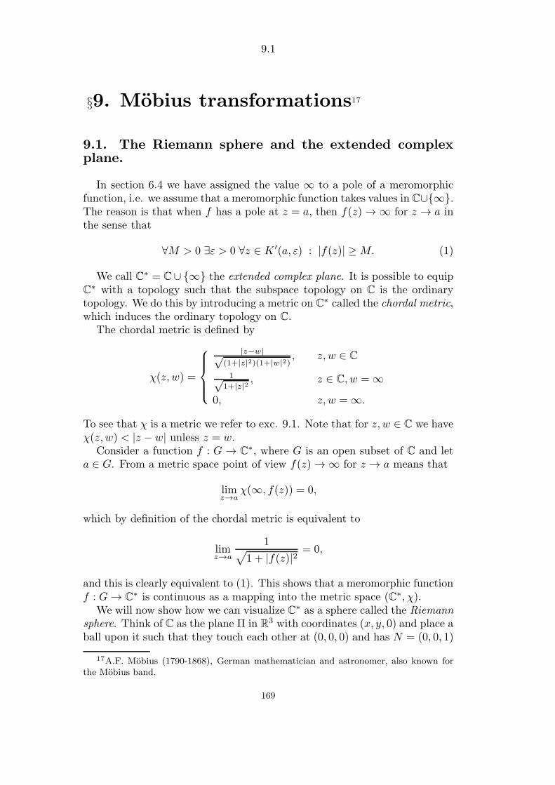
9.1

§9. Mobius transformations17

9.1. The Riemann sphere and the extended complexplane.

In section 6.4 we have assigned the value ∞ to a pole of a meromorphicfunction, i.e. we assume that a meromorphic function takes values in C∪∞.The reason is that when f has a pole at z = a, then f(z)→∞ for z → a inthe sense that

∀M > 0 ∃ε > 0 ∀z ∈ K ′(a, ε) : |f(z)| ≥M. (1)

We call C∗ = C∪ ∞ the extended complex plane. It is possible to equipC∗ with a topology such that the subspace topology on C is the ordinarytopology. We do this by introducing a metric on C∗ called the chordal metric,which induces the ordinary topology on C.

The chordal metric is defined by

χ(z, w) =

|z−w|√(1+|z|2)(1+|w|2)

, z, w ∈ C

1√1+|z|2

, z ∈ C, w =∞0, z, w =∞.

To see that χ is a metric we refer to exc. 9.1. Note that for z, w ∈ C we haveχ(z, w) < |z − w| unless z = w.

Consider a function f : G → C∗, where G is an open subset of C and leta ∈ G. From a metric space point of view f(z)→∞ for z → a means that

limz→a

χ(∞, f(z)) = 0,

which by definition of the chordal metric is equivalent to

limz→a

1√1 + |f(z)|2

= 0,

and this is clearly equivalent to (1). This shows that a meromorphic functionf : G→ C∗ is continuous as a mapping into the metric space (C∗, χ).

We will now show how we can visualize C∗ as a sphere called the Riemannsphere. Think of C as the plane Π in R3 with coordinates (x, y, 0) and place aball upon it such that they touch each other at (0, 0, 0) and has N = (0, 0, 1)

17A.F. Mobius (1790-1868), German mathematician and astronomer, also known for

the Mobius band.

169

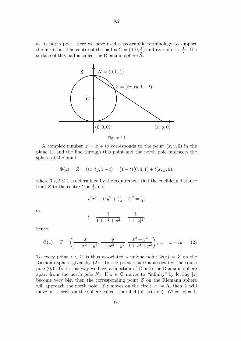
9.2

as its north pole. Here we have used a geographic terminology to supportthe intuition. The centre of the ball is C = (0, 0, 1

2) and its radius is 1

2. The

surface of this ball is called the Riemann sphere S.

•

S N = (0, 0, 1)

(0, 0, 0) (x, y, 0)

Z = (tx, ty, 1− t)

C

Figure 9.1

A complex number z = x + iy corresponds to the point (x, y, 0) in theplane Π, and the line through this point and the north pole intersects thesphere at the point

Φ(z) = Z = (tx, ty, 1− t) = (1− t)(0, 0, 1) + t(x, y, 0),

where 0 < t ≤ 1 is determined by the requirement that the euclidean distancefrom Z to the centre C is 1

2, i.e.

t2x2 + t2y2 + ( 12 − t)2 = 14 ,

or

t =1

1 + x2 + y2=

1

1 + |z|2 ,

hence

Φ(z) = Z =

(x

1 + x2 + y2,

y

1 + x2 + y2,

x2 + y2

1 + x2 + y2

), z = x+ iy. (2)

To every point z ∈ C is thus associated a unique point Φ(z) = Z on theRiemann sphere given by (2). To the point z = 0 is associated the southpole (0, 0, 0). In this way we have a bijection of C onto the Riemann sphereapart from the north pole N . If z ∈ C moves to “infinity” by letting |z|become very big, then the corresponding point Z on the Riemann spherewill approach the north pole. If z moves on the circle |z| = R, then Z willmove on a circle on the sphere called a parallel (of latitude). When |z| = 1,

170

9.3

then t = 12 and Z will move along the equator. For z, w ∈ C it is easy to

prove that χ(z, w) is the distance in space (=the length of the chord) betweenthe corresponding points Z,W on the sphere, cf. exc. 1. The length of thechord between the north pole N and Z is exactly the number 1/

√1 + |z|2.

In symbolsdist(Z,W ) = χ(z, w), z, w ∈ C∗, (3)

i.e. the mapping Φ : C∗ → S given by Φ(z) = Z,Φ(∞) = N is an isometryof (C∗, χ) onto S equipped with the restriction of the euclidean distance distin R3. Therefore (C∗, χ) is a compact metric space. In principle we shalldistinguish between the points of C∗ and S, but in many treatments of thetheory the extended complex plane is identified with the Riemann sphere.

The Riemann sphere is an important example of a compact Riemann sur-face.

The inverse mapping of Φ : C → S \ N is denoted σ and is called astereographic projection. From (2) we get that σ : S \ N → C is given by

σ(ξ, η, ζ) =ξ

1− ζ + iη

1− ζ , (ξ, η, ζ) ∈ S \ N. (4)

In fact, for (ξ, η, ζ) ∈ S\N we have 0 ≤ ζ < 1 so z = ξ/(1−ζ)+iη/(1−ζ) ∈C is well-defined. The equation of S can be written ξ2+η2 = ζ(1− ζ), hence

|z|2 =ξ2 + η2

(1− ζ)2 =ζ

1− ζ , 1 + |z|2 =1

1− ζ ,

and by (2) we finally get that Φ(z) = (ξ, η, ζ).

Theorem 9.1. The stereographic projection σ given by (4) maps circles onS \N into circles in C and circles on S passing through N into lines in C.

Proof. A circle on S is the intersection between S and a plane Σ. If the circleand hence the plane contains N , then its image under σ is the intersectionof the planes Σ and Π, hence a line in C.

Assume next that the plane Σ does not contain N . The equation of a planeΣ in R3 is the set of (ξ, η, ζ) ∈ R3 satisfying aξ + bη + cζ = d, where (a, b, c)is a unit vector in R3, a unit normal vector to Σ. Since N = (0, 0, 1) /∈ Σwe have c 6= d. Using that (ξ, η, ζ) = Φ(z) for z ∈ C, we get by (2) that thepoints z = x+ iy of σ(S ∩ Σ) satisfy

ax

1 + |z|2 + by

1 + |z|2 + c|z|2

1 + |z|2 = d,

hence (c− d)|z|2 + ax+ by = d, which for c 6= d is the equation of a circle inC.

171

9.4

Remark 9.2 It can also be proved that the stereographic projection σ isangle preserving in the following sense: Curves on S \ N intersecting eachother under an angle α are mapped to curves in C intersecting each otherunder the same angle. See Hille, Vol. I p. 41.

9.2. Mobius transformations.

The set of regular 2×2-matrices having complex entries is denoted GL2(C).To G ∈ GL2(C) we consider the expression

f(z) =M(G)(z) =az + b

cz + d, G =

(a bc d

). (1)

(Regularity of G just means that detG = ad − bc 6= 0.) Functions of thistype are called Mobius transformations or linear fractional transformations.

Let us consider some examples.

1) G =

(a 00 1

), a 6= 0.

The function is f(z) = az. The action of f is a homothetic transformationor a similitude with factor |a| followed by a rotation of size (angle) arg(a). Thehomothetic transformation is called a stretching if |a| > 1, and a contractionif |a| < 1. If |a| = 1 the action is a pure rotation. In all cases a figure ismapped to a figure of the same shape.

2) G =

(1 b0 1

), b ∈ C.

The function is f(z) = z+b. The action of f is a translation by the vectorb. Also in this case a figure is mapped onto a figure of the same shape.

In both cases we have limz→∞ f(z) = ∞, and defining f(∞) = ∞ weobtain that f is a bijection of C∗ onto itself and it is continuous on C∗. Theinverse mapping has the same form as f , namely f−1(z) = (1/a)z in thefirst case and f−1(z) = z − b in the second.

Therefore, in both cases f is a homeomorphism18 of C∗ onto itself.

3) G =

(0 11 0

).

The function is f(z) = 1/z. In this case f is a bijection of C \ 0, and itis its own inverse and is continuous. Since

limz→0

f(z) =∞, limz→∞

f(z) = 0,

it is reasonable to define f(0) = ∞, f(∞) = 0, hence f is a bijection of C∗.It is its own inverse and a homeomorphism.

18It is recalled that a mapping f : X → Y between topological spaces is called a

homeomorphism if f is a bijection and f as well as its inverse f−1 are continuous.

172

9.5

The action of f is an inversion in the unit circle reit → (1/r)eit followedby a reflection in the real axis z → z.

By the inversion in the unit circle all points of the circle are fixed, andeach open half-line emanating from zero is mapped onto itself in such a waythat points inside the unit circle are mapped to points outside the unit circleand vice versa.

We shall now see that the expression (1) defines a homeomorphism of C∗,and that it can be written as the composition of mappings of the type 1)-3).Notice that we assume ad− bc 6= 0.

If c = 0 then a, d 6= 0 and hence f(z) = (a/d)z + (b/d), which is acomposition of mappings of type 1) and 2), hence a homeomorphism of C∗.

If c 6= 0 we find

f(z) =(a/c)(cz + d) + b− ad/c

cz + d=a

c+

λ

cz + d, λ = −ad− bc

c,

which shows that f is equal to the composition of z → cz + d, z → 1/z andz → λz + a/c, hence f is a homeomorphism of C∗.

Summing up we have proved:

Theorem 9.3. The Mobius transformation (1) associated with the regularmatrix G is a homeomorphism of C∗ and the inverse mapping f−1 is againa Mobius transformation since

f(z) =az + b

cz + d= w ⇐⇒ f−1(w) =

dw − b−cw + a

= z. (2)

We have f(∞) = a/c, f(−d/c) = ∞ with the convention that the relevantfractions shall be understood as ∞, if the denominator c = 0.

Let Homeo(C*) denote the set of homeomorphisms of C∗. This set is agroup under composition of mappings, the neutral element being the identitymapping I of C∗.

Theorem 9.4. A Mobius transformation (1), which is not the identity ofC∗, has one or two fixed points in C∗.

Proof. The Mobius transformation (1) has z =∞ as a fixed point if and onlyif c = 0.

Assume first c = 0. Then f(z) = (a/d)z + b/d and if a 6= d then f hasthe additional fixed point z = b/(d− a). If a = d there are two possibilities:If b = 0 then f is the identity, and if b 6= 0 then f is a true translationf(z) = z + b/d with no fixed points other than z =∞.

Assume next c 6= 0. Then z ∈ C is a fixed point if and only if

cz2 + (d− a)z − b = 0,

which has one or two solutions.

173

9.6

Theorem 9.5. The mapping M : GL2(C) → Homeo(C*) defined by (1) isa group homomorphism such that

ker(M) := G ∈ GL2(C) |M(G) = I = (λ 00 λ

)| λ ∈ C \ 0.

Proof. For

G =

(a bc d

), H =

(α βγ δ

)∈ GL2(C)

we have

GH =

(aα+ bγ aβ + bδcα+ dγ cβ + dδ

),

hence

M(GH)(z) =(aα+ bγ)z + αβ + bδ

(cα+ dγ)z + cβ + dδ,

while

M(G) M(H)(z) =aαz+β

γz+δ + b

cαz+βγz+δ

+ d=a(αz + β) + b(γz + δ)

c(αz + β) + d(γz + δ),

which shows thatM(GH)(z) =M(G)M(H)(z), i.e. M is a homomorphismof groups.

If M(G) = I we have

az + b

cz + d= z for all z ∈ C, (3)

hence cz2+(d−a)z−b = 0 for all z ∈ C, but this is only possible if b = c = 0and a = d. On the other hand it is clear that all the diagonal matrices

G =

(λ 00 λ

)

with λ 6= 0 belong to GL2(C) and satisfy M(G) = I.A matrix G ∈ GL2(C) and all its non-zero multiples λG, λ 6= 0 determine

the same Mobius transformation. The theorem tells that if H ∈ GL2(C)determines the same Mobius transformation as G, then HG−1 ∈ ker(M)because M is a homomorphism, and hence H = λG for some λ 6= 0.

In Theorem 9.1 we have proved that circles on the Riemann sphere aremapped to either circles or lines in C under the stereographic projection.

This makes it convenient to introduce the following terminology:

174

9.7

Definition 9.6. A generalized circle Γ in C∗ is either a circle in C or a lineaugmented by ∞. We may consider a line as a circle through the point ∞.

With this definition we have:

Theorem 9.7. Every Mobius transformation maps a generalized circle ontoa generalized circle.

Proof. Using that every Mobius transformation can be composed of Mobiustransformations of the three types 1)-3) above, it suffices to prove the resultfor each of these types. The assertion being clear for the two first types,which in fact maps lines onto lines, circles onto circles, and leaves ∞ fixed,it suffices to prove it for the Mobius transformation f(z) = 1/z.

The equation of the circle ∂K(−a, r) can be written

|z + a|2 = r2, a ∈ C, r > 0,

hence|z|2 + az + az + |a|2 − r2 = 0, (4)

and the equation of a line can be written

αx+ βy + γ = 0, α, β, γ ∈ R, (α, β) 6= (0, 0),

or if we put a = (α+ iβ)/2 ∈ C \ 0

az + az + γ = 0. (5)

The equation for a generalized circle in C can therefore be written

δ|z|2 + az + az + γ = 0, δ, γ ∈ R, a ∈ C, (6)

with the assumption |a|2 > γδ. The case (4) corresponds to δ = 1, γ =|a|2 − r2, hence |a|2 > γδ. The case (5) corresponds to δ = 0, so |a|2 > γδalso holds in this case.

Conversely, the equation (6) with δ = 0 gives (5), while (6) with δ 6= 0gives

|z|2 + a

δz +

a

δz +

γ

δ= 0,

or

|z + a

δ|2 =

|a|2 − γδδ2

,

which describes a circle when |a|2 > γδ. The image of the generalized circle(6) under z → 1/z is determined in the following way: Dividing (6) by zzgives

δ +a

z+a

z+

γ

zz= 0

175

9.8

or with w = 1/zγ|w|2 + aw + aw + δ = 0, (7)

showing that w satisfies the equation of a generalized circle.If z = 0 belongs to the generalized circle (6) we have γ = 0, and then (7) is

the equation of a line. This corresponds to the fact that a generalized circlethrough 0 is mapped into a line under z → 1/z, a line being a generalizedcircle through infinity.

The following result is easy:Given 3 different points z1, z2, z3 ∈ C∗ there exists a uniquely determined

generalized circle Γ such that z1, z2, z3 ∈ Γ.

If one of the 3 points is ∞ then Γ is clearly a line through the two finitepoints. If z1, z2, z3 ∈ C then Γ is either a line or a circle. The case of a circleoccurs if z1, z2, z3 are the vertices of a non-degenerate triangle, and Γ is itscircumscribed circle.

Theorem 9.8. Let (z1, z2, z3), (w1, w2, w3) be two ordered triples of differentpoints in C∗. Then there exists one and only one Mobius transformationf : C∗ → C∗ such that f(zj) = wj , j = 1, 2, 3.

Proof. Assume first that w1 = 0, w2 = 1, w3 =∞.If z1, z2, z3 ∈ C, then f defined by

f(z) =(z2 − z3)(z − z1)(z2 − z1)(z − z3)

(8)

is a Mobius transformation with the desired properties. On the other hand,if a Mobius transformation f satisfies f(z1) = 0, then the numerator mustbe k(z − z1), and if f(z3) = ∞ the denominator must be l(z − z3). Finally,if f(z2) = 1 we get

f(z2) = 1 =k(z2 − z1)l(z2 − z3)

,

so f is given by (8).If z1 =∞, z2, z3 ∈ C, then

f(z) =z2 − z3z − z3

is a Mobius transformation mapping (∞, z2, z3) onto (0, 1,∞). It is also easyto see that this is the only possibility for f .

Similarly, if z1, z3 ∈ C, z2 =∞ (resp. z1, z2 ∈ C, z3 =∞), then

f(z) =z − z1z − z3

(resp. f(z) =

z − z1z2 − z1

)

176

9.9

are the only Mobius transformations with the desired properties.

Assume next that w1, w2, w3 are arbitrary different points in C∗.Let f, g be the Mobius transformations such that f maps (z1, z2, z3) onto

(0, 1,∞) and g maps (w1, w2, w3) onto (0, 1,∞). Then the composed Mobiustransformation g−1 f maps (z1, z2, z3) onto (w1, w2, w3).

Finally, if f, g both map (z1, z2, z3) onto (w1, w2, w3), then g−1 f has3 fixed points z1, z2, z3. By Theorem 9.4 we then get g−1 f = I, hencef = g.

Example 9.9. The Cayley transformation. The Mobius transformation

C(z) =z − iz + i

is called the Cayley transformation.C maps R ∪ ∞ onto the unit circle z ∈ C | |z| = 1, the upper half-

plane U onto the unit disc D = z ∈ C | |z| < 1 and the lower half-plane L

onto the exterior of the unit circle augmented by ∞.

To see this we calculate C(0) = −1, C(1) = −i, C(∞) = 1, so the ge-neralized circle determined by 0, 1,∞ (=the real line) is mapped onto thegeneralized circle determined by −1,−i, 1 (=the unit circle). Since C is abijection of C∗, U∪L must be mapped onto the complement of the unit circlein C∗, which consists of the interior and the exterior of the unit circle and thepoint ∞. Note that C(−i) =∞. We also know that C(U) and C(L \ −i)are domains in C by the open mapping theorem, and therefore C(U) has tobe either the interior or the exterior of the unit circle. In fact, if it containeda point A from the interior and a point B from the exterior of the unit circleit cannot be path connected, since a path from A to B would cross the unitcircle. Similarly C(L \ −i) has to be either the interior or the exterior ofthe unit circle. Since C(i) = 0 we conclude that C(U) = D. We can alsoargue that since C(−i) = ∞, then C(L \ −i) is an unbounded set, hencethe exterior of the unit circle.

Since C maps (i, 0,−i) onto (0,−1,∞) the imaginary axis is mapped tothe real axis. More precisely

C(iR) = (R \ 1) ∪ ∞.Notice also that the real and imaginary axis intersect each other at 0 underthe angle π/2, and since C′(0) = −2i the image curves intersect each other at−1 under the same angle by the results of section 1.2. In this case the imagecurves are the unit circle and the real axis and they intersect at -1 under theangle π/2. (The real and imaginary axis also intersect each other at infinitywhich corresponds to the intersection of the unit circle and the real axis at1. The two lines intersect at infinity under the angle π/2 if we look at thecorresponding circles on the Riemann sphere. They intersect each other atthe north pole under the angle π/2.)

177

9.10

Exercises for §9

9.1. The Riemann sphere S is defined as the sphere

(ξ, η, ζ) ∈ R3 | ξ2 + η2 + (ζ − 12 )

2 = 14.

To z = x+ iy ∈ C is associated the point Z ∈ S given by

Φ(z) = Z = (tx, ty, 1− t), t =1

1 + x2 + y2,

which is the intersection between S and the segment from N = (0, 0, 1) to(x, y, 0).

Prove that if w = u + iv ∈ C is another point corresponding to W ∈ Ssuch that

Φ(w) =W = (su, sv, 1− s), s =1

1 + u2 + v2,

then the euclidean distance dist(Z,W ) is equal to the chordal distance χ(z, w)from section 9.1. Prove also that

dist(N,Z) =1√

1 + x2 + y2, z ∈ C, N = (0, 0, 1).

Use this to prove that χ is a metric on C∗ and that the mapping Φ : C∗ → Sgiven by Φ(z) = Z,Φ(∞) = N is an isometry between metric spaces.

Explain why the spaces (C∗, χ) and (S, dist) are compact.

9.2. Prove that the Mobius transformation

f(z) =az + b

cz + d, G =

(a bc d

)∈ GL2(C)

satisfies

f ′(z) =detG

(cz + d)2, z ∈ C \ −d

c,

so f is conformal at all points of C \ −d/c, cf. Section 1.2.

9.3. Find the determinant of G ∈ GL2(C) defining the Mobius transforma-tion (8) in Section 9.2.

9.4. Consider the Mobius transformation f(z) = (1 + z)/(1− z) and provethat it maps the imaginary axis to the unit circle, the unit circle to theextended imaginary axis, and the extended real axis to itself.

178

9.11

Find the image of the domains

z ∈ C | |z| < 1, z ∈ C | |z| > 1

z ∈ C | |z| < 1,Re z > 0, z ∈ C | |z| < 1,Re z < 0.Show that the vertical line Re z = −1 is mapped to the circle ∂K(−1

2, 12)

and that the vertical strip z ∈ C | −1 < Re z < 0 is mapped onto K(0, 1) \K(−1

2 ,12).

9.5. Using the theory of Mobius transformations show that the transforma-tions fz0 given in (4) of Section 8 maps the unit circle circle onto itself andalso the unit disc onto itself. Show that the points

z0,1 + z01 + z0

,1

z0(1)

are mapped to 0, 1,∞. Prove that the generalized circle determined by (1)intersects the unit circle under an angle of π/2.

9.6. Let SL2(R) denote the set of 2 × 2 matrices of real numbers withdeterminant 1. Prove that the Mobius transformation f =M(G) given by amatrix G ∈ SL2(R) maps the upper half-plane onto itself.

9.7. Determine the fixed points of the Cayley transformation.

179

9.12

180

A.1

§A. Appendix

Various topological results

Lemma A.1. Let K,F ⊆ C be two non-empty closed and disjoint sets, andassume in addition that K is bounded. Then the distance d(K,F ) betweenK and F defined by

d(K,F ) = inf|z − w| | z ∈ K,w ∈ F

satisfies d(K,F ) > 0, and there exist points z′ ∈ K, w′ ∈ F such that|z′ − w′| = d(K,F ).

Proof. For any n ∈ N we can choose zn ∈ K, wn ∈ F satisfying

d(K,F ) ≤ |zn − wn| < d(K,F ) +1

n. (1)

Since K is bounded there exists R > 0 such that |z| ≤ R for all z ∈ K.We claim that also the sequence (wn) is bounded, because

|wn| = |wn−zn+zn| ≤ |wn−zn|+ |zn| < d(K,F )+1

n+R ≤ d(K,F )+1+R .

Since (zn) as well as (wn) are bounded, the sequence (zn, wn) ∈ C2 ≈ R4 hasa convergent subsequence (znp

, wnp) with limit (z′, w′) ∈ C2. By assumption

K and F are closed, hence z′ ∈ K, w′ ∈ F , and using the continuity of(z, w) 7→ |z − w| from C2 → R, we get

|znp− wnp

| → |z′ − w′| ,

which together with (1) gives

d(K,F ) = |z′ − w′| .

This number has to be > 0, for otherwise z′ = w′, which is then a point inK ∩ F , contradicting the assumption K ∩ F = ∅.

Remark A.2. Two closed and unbounded disjoint subsets of C can havethe distance 0. A simple example is F1 = R, F2 = x + i

x | x > 0, i.e. abranch of the hyperbola with the x-axis as an asymptote.

181

A.2

Theorem A.3. Let A ⊆ Rk be closed and bounded and let f : A → Rl becontinuous. Then the image f(A) is closed and bounded in Rl. In particularfor l = 1 the function f has a minimum and a maximum, i.e. there existpoints a1, a2 ∈ A such that

f(a1) = inf f(A), f(a2) = sup f(A).

Proof. In order to see that f(A) is closed, we consider a sequence x(n) fromA such that f(x(n)) → b. We shall prove that b ∈ f(A). By Bolzano-Weierstrass’s theorem there exist a ∈ A and a subsequence x(np) of x(n) suchthat x(np) → a. Using that f is continuous, we see that f(x(np)) → f(a).However, every subsequence of f(x(n)) tends to b, hence f(a) = b, i.e. b ∈f(A).

Assume next that f(A) is unbounded. For every n ∈ N we can then findx(n) ∈ A such that ‖f(x(n))‖ ≥ n. As before there exists a ∈ A and asubsequence x(np) such that x(np) → a, hence f(x(np)) → f(a) because ofthe continuity of f . By continuity of ‖ · ‖ we then get ‖f(x(np))‖ → ‖f(a)‖,but this contradicts ‖f(x(np))‖ ≥ np →∞.

In the special case l = 1 we have that f(A) is a closed and bounded subsetof R, hence inf f(A), sup f(A) ∈ f(A).

For a closed non-empty subset F of C we define dF : C→ [0,∞[ by

dF (z) = inf|z − a| | a ∈ F , (2)

called the distance from z to F .

Theorem A.4. The distance is a continuous function dF : C → [0,∞[satisfying

∀z ∈ C : dF (z) = 0 ⇐⇒ z ∈ F .

Proof. For z ∈ F we clearly have dF (z) ≤ |z − z| = 0. For z /∈ F it followsby Lemma A.1 that dF (z) = d(z, F ) > 0.

For z1, z2 ∈ C, a ∈ F we get by the triangle inequality

dF (z1) ≤ |z1 − a| ≤ |z1 − z2|+ |z2 − a| ,showing that dF (z1) − |z1 − z2| is a lower bound for the numbers |z2 − a|,a ∈ F . By the definition of infimum we then get

dF (z1)− |z1 − z2| ≤ dF (z2)or

dF (z1)− dF (z2) ≤ |z1 − z2| .Interchanging z1 and z2, we finally get

|dF (z1)− dF (z2)| ≤ |z1 − z2| ,which proves that dF is continuous (even diminishing distances).

182

A.3

Theorem A.5. To every open set G ⊆ C there exists an increasing sequenceK1 ⊆ K2 ⊆ . . . of closed and bounded subsets of G such that their union isG.

Proof. If G = C we can define Kn = z ∈ C | |z| ≤ n. If G 6= C we considerthe distance function d = dC\G, cf. (2) with F = C \G, and define

Fn =

z ∈ C | d(z) ≥ 1

n

= d−1

([1

n,∞[)

.

The continuity of d implies that Fn is closed, and since d(z) > 0 for z ∈ Fn

we have Fn ⊆ G. The sets

Kn = Fn ∩ z ∈ C | |z| ≤ n

form an increasing sequence of closed and bounded subsets of G. Any z ∈ Gbelongs to Kn for n sufficiently big because d(z) > 0.

Theorem A.6. Let A ⊆ C be path connected and assume that f : A→ C iscontinuous. Then the image set f(A) is path connected.

Proof. Two arbitrary points in f(A) can be written f(P ), f(Q), where P,Q ∈A. Let γ : [0, 1]→ A denote a continuous curve in A from P to Q. Then thecomposed function f γ is a continuous curve in f(A) from f(P ) to f(Q).

Theorem A.7. Let A ⊆ Rk and let B ⊆ Rl be closed and bounded. Iff : A×B → C is a continuous function, then for any x0 ∈ A

limx→x0

f(x, y) = f(x0, y), uniformly for y ∈ B,

i.e.

∀ε > 0 ∃δ > 0 ∀x ∈ A : ||x− x0|| < δ ⇒ ∀y ∈ B : |f(x, y)− f(x0, y)| < ε.

Proof. Given ε > 0 and a point (x0, y0) ∈ A × B, the continuity of f at(x0, y0) implies that there exist δ(x0, y0) > 0, r(x0, y0) > 0 such that for(x, y) ∈ A×B

||x− x0|| < δ(x0, y0), ||y − y0|| < r(x0, y0)⇒ |f(x, y)− f(x0, y0)| < ε/2.

The family of open balls K(y0, r(x0, y0)) | y0 ∈ B cover B, so by Borel’scovering Theorem 4.13 there exist finitely many points y1, y2, . . . , yn ∈ Bsuch that

B ⊆ ∪nj=1K(yj, r(x0, yj)).

183

A.4

Define δ(x0) = minδ(x0, yj) | j = 1, . . . , n and notice that δ(x0) > 0. Forx ∈ A such that ||x− x0|| < δ(x0) and for arbitrary y ∈ B we claim that

|f(x, y)− f(x0, y)| < ε. (3)

In fact, y ∈ K(yj, r(x0, yj)) for some j = 1, . . . , n because the balls cover B,and using ||x− x0|| < δ(x0) ≤ δ(x0, yj) we find

|f(x, y)− f(x0, yj)| < ε/2, |f(x0, y)− f(x0, yj)| < ε/2,

and (3) follows by the triangle inequality.

Remark A.8. In A.1, A.2, A.4, A.5, A.6 we can replace C by Rk for any k.

Countable and uncountable sets

Definition A.9. A set M is called countable, if there exists an injectivemapping f :M → N.

A set is called uncountable, if it is not countable.

In order for M to be countable we have to be able to assign a naturalnumber to each element of M in such a way that different elements of Mare assigned different numbers, like cloak-room tickets. This is what we aredoing when we count the elements in a finite set, so finite sets are countable.The set N, the set of even numbers and the set of square numbers are infinitecountable sets.

Theorem A.10. The sets Z,Q are countable and [0, 1]19 is uncountable.

Proof. Writing Z = 0, 1,−1, 2,−2, . . ., i.e. having placed the elements ofZ in a sequence such that each element appears once and only once, we seethat it is countable. A concrete injective mapping f : Z→ N, correspondingto this way of writing the set, can be defined by f(0) = 1, f(n) = 2n for n =1, 2, . . . , f(n) = 2|n|+ 1 for n = −1,−2, . . . .

We only prove that Q+ is countable, and the reader is asked to use this toprove that Q is countable. The following scheme contains all positive rationalnumbers, in fact they are all repeated infinitely many times.

19The same is true for every interval consisting of more than one point.

184

A.5

1 2 3 4 5

1/2 2/2 3/2 4/2 5/2

1/3 2/3 3/3 4/3 5/3

1/4 2/4 3/4 4/4 5/4

1/5 2/5 3/5 4/5 5/5

The injective mapping f : Q+ → N is now defined in the following way.We count diagonally by following the arrows, but if the number has alreadybeen counted, then it is skipped. We then have

f(1) = 1, f(1

2) = 2, f(2) = 3, f(

1

3) = 4, f(3) = 5, f(

1

4) = 6,

f(2

3) = 7, f(

3

2) = 8, f(4) = 9, f(

1

5) = 10, f(5) = 11, . . . .

We now reproduce the ingenious proof of Cantor for the result that [0, 1]is uncountable. Every number in [0, 1] can be written as an infinite decimalfraction 0, a1a2 . . . , where a1, a2 . . . ∈ 0, 1, 2, . . . , 9. If [0, 1] was countable,we could arrange the numbers from [0, 1] in a list, i.e. as a sequence of infinitedecimal fractions

0, a11a12a13 . . .

0, a21a22a23 . . .

0, a31a32a33 . . .

. . .

It is however easy to produce an infinite decimal fraction giving a numberin [0, 1] and which does not belong to the sequence, namely b = 0, b1b2 . . . ,where for each n the number bn is chosen among the digits 0, 1, 2, . . . , 9such that |bn − ann| ≥ 2. This procedure ensures that b is different from then’th number in the list for each n. (Note that e.g. 0, 0100 . . . = 0, 0099 . . . ,so we have to assume that the digits differ by 2 as above.)

Theorem A.11. Let A1, A2, . . . be a sequence of countable sets. Then M =∪∞1 An is countable.

The theorem is proved by exploiting the same idea of proof which wasused in establishing that Q+ is countable.

185

A.6

186

Bibliography

There exists a large number of elementary books on complex function the-ory because the subject is taught at all universities and engineering schools.In addition there are many research monographs treating selected topics fromcomplex analysis.

The present list is only a small selection in addition to the 3 books men-tioned in the introduction.

Ablowitz, M.J.; Fokas, A.S.: Complex Variables. Introduction and Applica-tions, 2003.

Ahlfors, Lars V.: Complex Analysis: an Introduction to the theory of AnalyticFunctions of one Complex Variable, 1979.

Bak, Joseph; Newman, Donald: Complex analysis, 1997.

Berenstein, Carlos A.; Gay, Roger: Comples variables. An introduction,1991.

Churchill, Ruel V.; Brown, James W.; Verhey, Roger, F.: Complex variablesand applications, 1974.

Conway, John B.: Functions of one complex variable, 1973.

Conway, John B.: Functions of one complex variable II, 1995.

Forster, Otto: Lectures on Riemann surfaces, 1981.

Hayman, W.K.: Multivalent functions, 1958.

Jameson, G.J.O.: A first course on complex functions, 1970.

Kodaira, Kunihiko: Introduction to complex analysis, 1984.

Lang, Serge: Complex analysis, 1999.

Littlewood, J.E.: Lectures on the theory of functions, 1944.

Marsden, Jerrold E.: Basic complex analysis, 1973.

Narasimhan, Raghavan: Complex analysis in one variable, 1985.

Remmert, Reinhold: Classical topics in complex function theory, 1998.

Stewart, Ian; Tall, David: Complex Analysis, 1983.

187

LIST OF SYMBOLS

N = 1, 2, 3, . . . The natural numbersN0 = 0, 1, 2, 3, . . . The natural numbers and 0Z = 0,±1,±2, . . . The integersQ The rational numbersR The real numbersC The complex numbers i.1arg The argument 5.5Arg The principal argument 5.5Argα 5.5argvar Variation of argument 5.8Aut(G) Automorphism group of G 8.4C∗ Extended complex plane 9.1C[z] Polynomials 4.17C(z) Rational functions 6.8χ(z, w); The chordal metric; 9.1fe 6.17fi 6.17GL2(C) 9.4H(G) Holomorphic functions in G 1.1Homeo(C∗) 9.5K(a, r) Open disc or ball i.1K ′(a, r) i.1L(γ) Length of path 2.6ln; The natural logarithmlog Multi-valued logarithm 5.11Log Principal logarithm 5.11Log α 5.12M(G) Meromorphic functions in G 6.11M(G); Mobius transformation associated to G 9.4∫γ,∫γf 2.4

Mf (r); The maximum modulus 8.2ω(γ, 0); The winding number around 0 5.8, 5.17ω(γ, z); The winding number around z 5.20ord(f, a) Order of zero 6.2Res(f, a) Residue 7.1sign (A) Signature 5.18SL2(R) 9.11Z(f); Zero set of f ; 6.3

188

INDEX

A

accumulation point 5.3

algebra, fundamental theorem of 4.16

analytic function 4.8

annulus 6.14

arccos function 5.5

arcsin function 5.16

arctan function 3.14, 5.5

argument i.1, 5.5

argument function 5.5

argument, principle of 7.4

argument, variation of 5.8

automorphism group Aut(G) 8.4

B

Bernoulli numbers 6.25, 6.26, 7.22

Bessel functions 6.25

biholomorphic 5.15

binomial series 5.14

Binet’s formula 6.26

Borel’s covering theorem 4.11

branch point 5.9

C

C1-curve 2.3

Casorati-Weierstrass’ theorem 6.7

Cauchy-Riemann’s differential equations 1.6

Cauchy’s integral theorem 3.3, 3.6

Cauchy’s integral formula 3.9

Cauchy’s integral formula for derivatives

4.7

Cauchy multiplication 5.25

Cauchy’s residue theorem 7.1

Cayley transformation 9.9

chordal metric 9.1

cluster point 5.3

complex differentiable 1.1

complex number i.1

component 5.20, 5.23

conformal 1.5

conformal mapping 1.5

conjugate harmonic function 4.10

connected component 5.20, 5.23

continuous curve 2.2

contour 2.6

contour integral 2.3

contraction 9.4

convex 3.2

cosine function 1.15

cotangent function 1.18

countable 5.3, A.4curve

- closed 2.2

- continuous 2.2- Jordan 2.3

- oriented continuous 2.2- reverse 2.3

- simple 2.3

- smooth 2.3

D

decomposition, partial fraction 6.9derivative 1.1

differentiable, complex 1.1

discrete set 5.3division of polynomials 4.17

domain 1.8, 5.2- annular=annulus 6.14

- simply connected 3.1

- star-shaped 3.1

E

elliptic function 5.17elliptic integral 5.17

entire function 4.15

estimation lemma 2.6Euler’s formulas 1.15

Euler’s partial fraction decomposition 7.18

exponential function 1.13extended complex plane 9.1

F

Fibonacci–numbers 6.26

Fresnel’s integrals 3.15

fundamental theorem of algebra 4.16

G

generalized circle 9.7Goursat’s lemma 3.3

H

harmonic function 4.9

holomorphic function 1.1

holomorphic branch 5.9, 5.12, 5.14homeomorphism 9.4

homothetic transformation 9.4homotopy 3.1

hyperbolic functions 1.18

189

I

identity theorem

- for holomorphic fcts. 6.4

- for power series 1.12imaginary part i.1

indeterminate moment problem 7.22

integral along C1-curve 2.3integral along a path 2.6

inversion 9.5isolated point 5.3

isolated singularity 6.5

J

Jacobian 1.8

Jordan curve 2.3

Jordan’s theorem 2.3

L

Laplace operator 4.9Laurent series 6.13

Leibniz’ formula 1.22

length of path 2.6l’Hospitals rule 6.4

linear fractional transformation 9.4

Liouville’s theorem 4.16local uniform convergence 4.11

M

maximum modulus principle

- global version 8.2

- local version 8.1meromorphic function 6.11

modulus i.1Morera’s theorem 4.11

Mobius transformation 9.4

N

numerical value i.1

O

open mapping theorem 7.7

order

- pole 6.6- zero 6.2

P

parameterization 2.2partial fraction decomposition 6.9

path 2.6path connected 5.1

path integral 2.3

paving lemma 5.2

Picard’s theorem 4.16

Picard’s great theorem 6.7

pointwise convergence 4.1

polar coordinates i.1

pole 6.6

polynomials 4.16

powers 5.13

primitive 2.7

principal argument 5.5

principal logarithm 5.11, exc. 3.6

principal part 6.7, 6.19

R

radius of convergence 1.9

rational function 6.8

real part i.1

reflection principle 6.23

residue 7.1

Riemann’s mapping theorem 5.15

Riemann sphere 9.1

Riemann surface 5.1, 5.10

Riemann’s ζ-function 4.23

Rouche’s theorem 7.6

rotation angle 1.6

S

Schwarz’ lemma 8.3

sequence of functions 4.1

- local uniform convergence 4.11

- pointwise convergence 4.1

- uniform convergence 4.2

signature 5.18

similitude 9.4

simple pole 6.6

simple zero 6.2

simply connected 3.1

sine function 1.15

singularity

- essential 6.6

- isolated 6.5

- removable 6.5

speed 2.3

staircase line 1.8

star-shaped 3.1

stereographic projection 9.3

stretching 9.4

T

tangent function 1.18

Taylor series 4.6

190

transcendental entire function 6.20

translation 9.4

trigonometric functions 1.15

U

uncountable A.4

uniform convergence 4.2

W

Weierstrass’ M-test 4.4

winding number 5.8, 5.20

Z

zero 6.1

191

192