Welcome message from author
This document is posted to help you gain knowledge. Please leave a comment to let me know what you think about it! Share it to your friends and learn new things together.
Transcript


Complex Analysis
Second edition
This new edition of a classic textbook develops complex analysis from the establishedtheory of real analysis by emphasising the differences that arise as a result of the richergeometry of the complex plane. Key features of the authors’ approach are to use simpletopological ideas to translate visual intuition into rigorous proof, and, in this edition, toaddress the conceptual conflicts between pure and applied approaches head-on.Beyond the material of the clarified and corrected original edition, there are three
new chapters: Chapter 15 on infinitesimals in real and complex analysis; Chapter 16 onhomology versions of Cauchy’s Theorem and Cauchy’s Residue Theorem, linking backto geometric intuition; and Chapter 17 outlines some more advanced directions in whichcomplex analysis has developed, and continues to evolve into the future.With numerous worked examples and exercises, clear and direct proofs, and a view
to the future of the subject, this is an invaluable companion for any modern complexanalysis course.
Ian Stewart, FRS is Emeritus Professor of Mathematics at the University of Warwick. Heis author or coauthor of over 190 research papers and is the bestselling author of over120 books, from research monographs and textbooks to popular science and science fic-tion. His awards include the Royal Society’s Faraday Medal, the IMA Gold Medal,the AAAS Public Understanding of Science Award, the LMS/IMA Zeeman Medal,the Lewis Thomas Prize, and the Euler Book Prize. He is an honorary wizard of theDiscworld’s Unseen University.
David Tall is Emeritus Professor of Mathematical Thinking at the University of War-wick and is known internationally for his contributions to mathematics education. He isauthor or coauthor of over 200 papers and 40 books and educational computer software,covering all levels from early childhood to research mathematics.

Complex Analysis(The Hitch Hiker’s Guide to the Plane)
Second edition
IAN STEWART
DAVID TALL
University of Warwick

University Printing House, Cambridge CB2 8BS, United Kingdom
One Liberty Plaza, 20th Floor, New York, NY 10006, USA
477 Williamstown Road, Port Melbourne, VIC 3207, Australia
314–321, 3rd Floor, Plot 3, Splendor Forum, Jasola District Centre, New Delhi – 110025, India
79 Anson Road, #06–04/06, Singapore 079906
Cambridge University Press is part of the University of Cambridge.
It furthers the University’s mission by disseminating knowledge in the pursuit ofeducation, learning, and research at the highest international levels of excellence.
www.cambridge.orgInformation on this title: www.cambridge.org/9781108436793DOI: 10.1017/9781108505468
First edition c± Cambridge University Press 1983Second edition c± JOAT Enterprises and David Tall 2018
This publication is in copyright. Subject to statutory exceptionand to the provisions of relevant collective licensing agreements,no reproduction of any part may take place without the writtenpermission of Cambridge University Press.
First published 1983Thirteenth reprint 2004Second edition 2018
Printed in the United Kingdom by TJ International Ltd, Padstow, Cornwall 2018
A catalogue record for this publication is available from the British Library.
Library of Congress Cataloging-in-Publication DataNames: Stewart, Ian, 1945– author. | Tall, David Orme, author.Title: Complex analysis : the hitch hiker’s guide to the plane / Ian Stewart(University of Warwick), David Tall (University of Warwick).
Other titles: Hitch hiker’s guide to the planeDescription: Second edition. | Cambridge : Cambridge University Press, 2018.| Includes bibliographical references and index.
Identifiers: LCCN 2018007009 | ISBN 9781108436793 (alk. paper)Subjects: LCSH: Functions of complex variables. | Numbers, Complex. |Geometry, Analytic–Plane.
Classification: LCC QA331 .S85 2018 | DDC 515/.9–dc23LC record available at https://lccn.loc.gov/2018007009
ISBN 978-1-108-43679-3 Paperback
Additional resources for this publication at www.cambridge.org/Stewart&Tall2ed
Cambridge University Press has no responsibility for the persistence or accuracyof URLs for external or third-party internet websites referred to in this publicationand does not guarantee that any content on such websites is, or will remain,accurate or appropriate.

Contents
Preface to the Second Edition page xi
Preface to the First Edition xiv
0 The Origins of Complex Analysis, and Its Challenge to Intuition 1
0.1 The Origins of Complex Numbers 1
0.2 The Origins of Complex Analysis 5
0.3 The Puzzle 6
0.4 Is Mathematics Discovered or Invented? 7
0.5 Overview of the Book 10
1 Algebra of the Complex Plane 13
1.1 Construction of the Complex Numbers 13
1.2 The x+ iyNotation 15
1.3 A Geometric Interpretation 16
1.4 Real and Imaginary Parts 17
1.5 The Modulus 17
1.6 The Complex Conjugate 18
1.7 Polar Coordinates 19
1.8 The Complex Numbers Cannot be Ordered 20
1.9 Exercises 21
2 Topology of the Complex Plane 24
2.1 Open and Closed Sets 26
2.2 Limits of Functions 27
2.3 Continuity 30
2.4 Paths 35
2.4.1 Standard Paths 35
2.4.2 Visualising Paths 37
2.4.3 The Image of a Path 37
2.5 Change of Parameter 38
2.5.1 Preserving Direction 39
2.6 Subpaths and Sums of Paths 39
2.7 The Paving Lemma 43

vi Contents
2.8 Connectedness 46
2.9 Space-filling Curves 52
2.10 Exercises 55
3 Power Series 59
3.1 Sequences 59
3.2 Series 63
3.3 Power Series 66
3.4 Manipulating Power Series 69
3.5 Products of Series 71
3.6 Exercises 72
4 Differentiation 75
4.1 Basic Results 75
4.2 The Cauchy–Riemann Equations 78
4.3 Connected Sets and Differentiability 82
4.4 Hybrid Functions 83
4.5 Power Series 84
4.6 A Glimpse Into the Future 87
4.6.1 Real Functions Differentiable Only Finitely Many Times 87
4.6.2 Bad Behaviour of Real Taylor Series 88
4.6.3 The Blancmange function 89
4.6.4 Complex Analysis is Better Behaved 91
4.7 Exercises 92
5 The Exponential Function 96
5.1 The Exponential Function 96
5.2 Real Exponentials and Logarithms 98
5.3 Trigonometric Functions 99
5.4 An Analytic Definition of π 100
5.5 The Behaviour of Real Trigonometric Functions 101
5.6 Dynamic Explanation of Euler’s Formula 103
5.7 Complex Exponential and Trigonometric Functions are Periodic 104
5.8 Other Trigonometric Functions 105
5.9 Hyperbolic Functions 106
5.10 Exercises 107
6 Integration 111
6.1 The Real Case 112
6.2 Complex Integration Along a Smooth Path 113
6.3 The Length of a Path 117
6.3.1 Integral Formula for the Length of Smooth Paths and Contours 119
6.4 If You Took the Short Cut . . . 122
6.5 Further Properties of Lengths 122

Contents vii
6.5.1 Lengths of More General Paths 123
6.6 Regular Paths and Curves 124
6.6.1 Parametrisation by Arc Length 126
6.7 Regular and Singular Points 127
6.8 Contour Integration 130
6.8.1 Definition of Contour Integral 131
6.9 The Fundamental Theorem of Contour Integration 133
6.10 An Integral that Depends on the Path 136
6.11 The Gamma Function 137
6.11.1 Known Properties of the Gamma Function 139
6.12 The Estimation Lemma 140
6.13 Consequences of the Fundamental Theorem 143
6.14 Exercises 146
7 Angles, Logarithms, and the Winding Number 149
7.1 Radian Measure of Angles 150
7.2 The Argument of a Complex Number 151
7.3 The Complex Logarithm 153
7.4 The Winding Number 155
7.5 The Winding Number as an Integral 159
7.6 The Winding Number Round an Arbitrary Point 159
7.7 Components of the Complement of a Path 160
7.8 Computing the Winding Number by Eye 161
7.9 Exercises 164
8 Cauchy’s Theorem 169
8.1 The Cauchy Theorem for a Triangle 171
8.2 Existence of an Antiderivative in a Star Domain 173
8.3 An Example – the Logarithm 175
8.4 Local Existence of an Antiderivative 176
8.5 Cauchy’s Theorem 177
8.6 Applications of Cauchy’s Theorem 180
8.6.1 Cuts and Jordan Contours 181
8.7 Simply Connected Domains 183
8.8 Exercises 184
9 Homotopy Versions of Cauchy’s Theorem 187
9.1 Informal Description of Homotopy 187
9.2 Integration Along Arbitrary Paths 189
9.3 The Cauchy Theorem for a Boundary 191
9.4 Formal Definition of Homotopy 195
9.5 Fixed End Point Homotopy 197
9.6 Closed Path Homotopy 198
9.7 Converse to Cauchy’s Theorem 201

viii Contents
9.8 The Cauchy Theorems Compared 202
9.9 Exercises 204
10 Taylor Series 207
10.1 Cauchy Integral Formula 208
10.2 Taylor Series 209
10.3 Morera’s Theorem 212
10.4 Cauchy’s Estimate 213
10.5 Zeros 214
10.6 Extension Functions 217
10.7 Local Maxima and Minima 219
10.8 The Maximum Modulus Theorem 220
10.9 Exercises 221
11 Laurent Series 225
11.1 Series Involving Negative Powers 225
11.2 Isolated Singularities 230
11.3 Behaviour Near an Isolated Singularity 232
11.4 The Extended Complex Plane, or Riemann Sphere 234
11.5 Behaviour of a Differentiable Function at Infinity 236
11.6 Meromorphic Functions 237
11.7 Exercises 239
12 Residues 243
12.1 Cauchy’s Residue Theorem 243
12.2 Calculating Residues 246
12.3 Evaluation of Definite Integrals 248
12.4 Summation of Series 258
12.5 Counting Zeros 261
12.6 Exercises 263
13 Conformal Transformations 268
13.1 Measurement of Angles 268
13.1.1 Real Numbers Modulo 2π 268
13.1.2 Geometry of R/2π 269
13.1.3 Operations on Angles 270
13.1.4 The Argument Modulo 2π 270
13.2 Conformal Transformations 271
13.3 Critical Points 276
13.4 Möbius Maps 278
13.4.1 Möbius Maps Preserve Circles 278
13.4.2 Classification of Möbius Maps 279
13.4.3 Extension of Möbius Maps to the Riemann Sphere 281
13.5 Potential Theory 281

Contents ix
13.5.1 Laplace’s Equation 281
13.5.2 Design of Aerofoils 283
13.6 Exercises 284
14 Analytic Continuation 289
14.1 The Limitations of Power Series 289
14.2 Comparing Power Series 291
14.3 Analytic Continuation 293
14.3.1 Direct Analytic Continuation 293
14.3.2 Indirect Analytic Continuation 295
14.3.3 Complete Analytic Functions 296
14.4 Multiform Functions 296
14.4.1 The Logarithm as a Multiform Function 297
14.4.2 Singularities 298
14.5 Riemann Surfaces 299
14.5.1 Riemann Surface for the Logarithm 299
14.5.2 Riemann Surface for the Square Root 300
14.5.3 Constructing a General Riemann Surface by Gluing 301
14.6 Complex Powers 302
14.7 Conformal Maps Using Multiform Functions 304
14.8 Contour Integration of Multiform Functions 305
14.9 Exercises 311
15 Infinitesimals in Real and Complex Analysis 315
15.1 Infinitesimals 316
15.2 The Relationship Between Real and Complex Analysis 318
15.2.1 Critical Points 320
15.3 Interpreting Power Series Tending to Zero as Infinitesimals 322
15.4 Real Infinitesimals as Variable Points on a Number Line 323
15.5 Infinitesimals as Elements of an Ordered Field 324
15.6 Structure Theorem for any Ordered Extension Field of R 327
15.7 Visualising Infinitesimals as Points on a Number Line 328
15.8 Complex Infinitesimals 331
15.9 Non-standard Analysis and Hyperreals 333
15.10 Outline of the Construction of Hyperreal Numbers 336
15.11 Hypercomplex Numbers 337
15.12 The Evolution of Meaning in Real and Complex Analysis 341
15.12.1 A Brief History 341
15.12.2 Non-standard Analysis in Mathematics Education 342
15.12.3 Human Visual Senses 344
15.12.4 Computer Graphics 345
15.12.5 Summary 346
15.13 Exercises 346

x Contents
16 Homology Version of Cauchy’s Theorem 350
16.0.1 Outline of Chapter 351
16.0.2 Group-theoretic Interpretation 353
16.1 Chains 354
16.2 Cycles 356
16.2.1 Sums and Formal Sums of Paths 357
16.3 Boundaries 358
16.4 Homology 360
16.5 Proof of Cauchy’s Theorem, Homology Version 362
16.5.1 Grid of Rectangles 363
16.5.2 Proof of Theorem 16.2 365
16.5.3 Rerouting Segments 366
16.5.4 Resumption of Proof of Theorem 16.2 368
16.6 Cauchy’s Residue Theorem, Homology Version 368
16.7 Exercises 370
17 The Road Goes Ever On . . . 374
17.1 The Riemann Hypothesis 374
17.2 Modular Functions 377
17.3 Several Complex Variables 378
17.4 Complex Manifolds 379
17.5 Complex Dynamics 379
17.6 Epilogue 381
References 382
Index 383

Preface to the Second Edition
The first edition of Complex Analysis focused on generalising concepts from real analy-sis to the complex case. Where there were differences, we looked at the geometric
picture to see why they were happening. This second edition does the same, but it alsofocuses on the increasing sophistication of mathematical ideas as we build from intuitionto rigour, in a manner where greater understanding leads to more sophisticated intuitionsand ways of working. New concepts and methods often start out in a technical way, withproblematic aspects that conflict with intuition. As well as generalising real analysis, wemove beyond it by addressing these conceptual conflicts, resolving them, and providingmore sophisticated concepts and methods appropriate to complex analytic functions.This approach is used throughout the book. So, for example, the text now includes a
short (but complete) discussion of the construction of a space-filling curve, to challengeour intuition about continuity and to explain why we have had to be careful with topo-logical assertions that appear obvious. The treatment here is simpler than most of theliterature on space-filling curves. We have spent some time examining different notionsof a path, especially the role of smoothness.
We have added three new chapters. Chapter 15 introduces ideas about infinitesimals
in real and complex analysis, thought of as variables that tend to zero, and formulated
as elements of extensions of the real and complex fields. Chapter 16 gives a formal linkfrom analysis back to geometric intuition, formulating and proving homology versionsof Cauchy’s Theorem and Cauchy’s Residue Theorem. Chapter 17 outlines a few of themore advanced directions in which complex analysis has developed, and continues toevolve into the future.Chapter 15 has been added for the following reasons. Since the first edition appeared
in 1983, the ways in which we operate mathematically have changed dramatically. Notonly are there computers that perform numerical and symbolic operations at a speedway beyond that previously available to the individual mind; there are also interactivegraphics drawn on high-resolution screens that let us visualise mathematical ideas incompletely new ways. In particular, we can dynamically magnify pictures to see tinydetail that lets us represent ‘arbitrarily small’ quantities.This second edition therefore includes an extra chapter to introduce formally defined
infinitesimals that lie in an ordered extension field K of the real numbers, which canbe manipulated algebraically and visualised formally on an extended number line. Thisapproach generalises to the complex case using the field K(i) where i2 = −1, which

xii Preface to the Second Edition
can be visualised in the extended complex plane. This construction offers a meaningfulbridge between the epsilon-delta rigour of pure mathematics and the intuitive use ofinfinitesimals in applications.It can easily be shown that any proper ordered field extension K of the reals must
contain infinitesimal elements x: that is, elements that are not zero yet satisfy |x| < r
for all positive real numbers r. Using the completeness of the real numbers, we prove asimple theorem that any finite element of K has the form k = c+ h, where c is real andh is infinitesimal or zero. A transformation in the form m(x) = (x − c)/ε, where ε is apositive infinitesimal, then lets us magnify infinitesimal detail near c and see it with ourunaided human eyes in a real picture. This technique extends to the complex case in thefield K(i).
We can now illustrate why complex analysis is so different from real analysis. Adifferentiable complex function defined on an open set is locally expressible as a powerseries, and we may take K to be the smallest ordered extension field generated by asingle infinitesimal ε. The elements are power series
∑r≥n a
rεr in ε with possibly afinite number of terms in 1/ε, and each non-zero element has an order of infinitesimalityn related to the first non-zero coefficient an (where the element may be infinite if nis negative). Meanwhile a differentiable real function may be differentiable once butnot twice, and this requires a much more sophisticated extension field K such as thatgiven by the logical theory of non-standard analysis. While Gottfried Leibniz imaginedinfinitesimals of different orders, non-standard analysis fails to have this property andrequires a much more sophisticated construction. At the end of the chapter we compareand contrast the various theories within a single framework.Chapter 16 on homology complements Chapter 9 on homotopy versions of Cauchy’s
Theorem, and logically it could have been placed immediately after that. We postponeit to the penultimate chapter because we do not wish to delay the more practical payofffrom Cauchy’s Theorem – Taylor and Laurent series, residues, evaluation of integrals,summation of series, and so on.Homology can be thought of as a way of characterising ‘holes’ in a topological space,
which here is the domain of a complex function f . Singularities, where f is not differ-entiable, create such holes, and homology helps to describe the topological effect ofsingularities; for example, in the homology version of Cauchy’s Residue Theorem. Toavoid including big chunks of algebraic topology, our approach to homology is based onstep paths in open subsets of the plane, one of the main simplifying tools in this book.The proof is ‘bare hands’ and exploits the simple geometry of step paths and the abeliangroup structure of homology.Chapter 17 has been included to make it clear that complex analysis is still a major
area of mathematical research. Complete though the classical theory may seem to be,there are numerous generalisations and new questions. The main topics mentioned arethe Riemann Hypothesis, modular functions, several complex variables, complex man-ifolds, and complex dynamics – leading to the fractal geometry of Julia sets and thefamous Mandelbrot set.In this new edition of Complex Analysis we have corrected all known typographical
errors, simplifed some proofs, and reorganised the material in mostly harmless ways to

Preface to the Second Edition xiii
improve readability. We have brought the text and layout into line with current practice,and redrawn all the figures. Proofs, definitions, and examples are terminated with the‘end of proof’ symbol ±. The same symbol indicates the absence of a proof when theresult is clear or has already been proved. Contrary to the prevailing wisdom, we donot insert punctuation marks at the end of displayed formulas. (Your tutors may objectto this. Tradition is on their side. If they do, they can set you an extra exercise: insertall missing punctuation.) But it is now the twenty-first century. No one puts full stops(US: periods) at the end of book titles, or chapter or section headings. So why do this indisplayed formulas, where it may cause confusion because punctuation marks are alsooften part of the symbolism? We suggest that clean typography should override pedanticpunctuation.
Formulas in the main text are another matter; here the absence of punctuation cancause confusion. We have followed tradition here.
Online Supplementary Material
Supplementary material including a concordance showing in more detail the changesbetween the previous edition and this one, and links to GeoGebra, can be found on theCambridge University Press website: www.cambridge.org/Stewart&Tall2ed.

Preface to the First Edition
Students faced with a course on ‘Complex Analysis’ often find it to be just that –complex. In the sense of ‘complicated’.
It’s true, of course, that the proofs of some of the major theorems in the subject candemand a certain technical versatility. But in many ways, on a conceptual level, complex
analysis is actually easier than real analysis; it just isn’t always taught that way.This book is intended for use at the level of second or third year undergraduates,
and it is based on experience accumulated from teaching such courses over the pastdecade. To exhibit the inherent simplicity of complex analysis we have organised thematerial around two basic principles: (1) generalise from the real case, and (2) whenthat reveals new phenomena, use the rich geometry of the plane to understand them.
Our aim throughout is to encourage geometric thinking, with the proviso that it must beadequately backed by analytic rigour.The opening chapter sets the work in its historical context, and the history is often
alluded to later as partial motivation. However, we feel that cultural changes often affectthe status of conceptual problems: what was once an important difficulty can become
a triviality when viewed with hindsight. It is not always necessary to drag today’s stu-dents through yesterday’s hang-ups. We argue the point at greater length below: it isfundamental to our entire approach.

0 The Origins of Complex Analysis, andIts Challenge to Intuition
In a lecture in 1886, Leopold Kronecker asserted that the integers are made by God andall the rest is the work of Man (Gray [7]). If so, complex numbers are certainly oneof humanity’s most intriguing mathematical artefacts. For centuries they have been awonder to mathematicians and philosophers alike. It took nearly 300 years from theirfirst appearance in Girolamo Cardano’s Ars Magna (The Great Art) to the publicationof a formal definition that satisfies modern standards of rigour. Building on such foun-dations, the initiated reader might be forgiven for thinking that complex analysis mustbe an incredibly complicated theory. Yet here we come to a historical puzzle. Althoughit took nearly three centuries to obtain a satisfactory treatment of complex numbers, itthen took less than a tenth of that time to complete a major part of complex analysis,
which is far more sophisticated and extensive.Obviously the numbers must come first, or there is nothing to do analysis with, but
the timescale is surprising. A possible explanation is that setting up the foundationsadequately involved deep problems of a philosophical nature: it took a long time to cometo grips with them, but once the ‘breakthrough’ had occurred, the further developmentwas easy by comparison.History suggests otherwise.
0.1 The Origins of Complex Numbers
Cardano’s celebrated Ars Magna of 1545 is one of the most important early alge-bra texts. Diophantus’s Arithmetica of about 250 discussed the solution of equationsand introduced a rudimentary form of algebraic notation. Muhammad al-Khwarizmi’sAl-kitab al-mukhtasar fi hisab al-gabr wa’l-muqabala (The Compendious Book on Cal-culation by Completion and Balancing) appeared around 820. Its translation into Latinas Liber Algebrae et Almucabola gave us the word ‘algebra’. Al-Khwarizmi’s discussionwas verbal, with no symbols but occasional diagrams.Cardano introduced a systematic algebraic notation, very different from what we use
today. He used this to present the newly discovered solutions of cubic and quartic equa-tions. His book contained the solution of cubics discovered by Scipione del Ferro around1500, and independently by Niccolo Fontana (nicknamed ‘Tartaglia’, the stammerer)around 1535. The high point of the text is the solution of quartic equations found byCardano’s student Lodovico Ferrari. The tangled tale of alleged duplicity and public

2 The Origins of Complex Analysis, and Its Challenge to Intuition
controversy that accompanied these discoveries can be found in Stewart [19, 20] andother historical sources.Ars Magna also discussed the simultaneous equations
x+ y = 10
xy= 40
and obtained a solution (in modern notation) of the form
x = 5+√−15 y = 5−
√−15
Cardano gave no interpretation for the square root of a negative number, but he didobserve that, on the assumption that the quantities obey the usual algebraic rules, wecan check that they satisfy the equations. His attitude to the discovery was dismissive:
‘So progresses arithmetic subtlety, the end of which . . . is as refined as it is useless.’In the same book he observed that applying Tartaglia’s formula to the cubic equation
x3 = 15x+ 4 (0.1)
leads to the solution
x = 3
±2+
√−121+ 3
±2−
√−121
in contrast to the obvious answer x = 4.
In both instances there was a conflict between the intuition about numbers that math-
ematicians had built up over the years, and the formal behaviour of the symbolic
manipulations that Cardano was carrying out. It took centuries for mathematicians toextend the number concept and develop a refined intuition in which Cardano’s obser-vations make sense. The first step happened not long after, however. Raphael Bombelli
(1526–73) suggested a way to reconcile the two solutions of (0.1) by manipulating the‘impossible’ roots as if they are ordinary numbers. Since
(2±√−1)3 = 2±
√−121
Cardano’s expression becomes
x = (2+√−1) + (2−
√−1) = 4
and the ‘impossible’ root is just the familiar root in a complex disguise. Bombelli’s workwas the first hint that complex numbers can prove useful in solving real mathematical
problems. But the message took a long time to sink in.In La Géometrie (1637), René Descartes made the distinction between ‘real’ and
‘imaginary’ numbers, interpreting the occurrence of imaginaries as a sign that the prob-lem concerned is insoluble, an opinion shared by Isaac Newton at a later date. However,this view sits uneasily with Bombelli’s realisation that a formula involving complex
numbers sometimes leads to a real solution, suggesting that the issue is not that simple.
John Wallis [25] represented a complex number geometrically in his Algebra of 1685.On a fixed line the real part of the number was measured off (in the direction given byits sign); then the imaginary part was measured off at right angles, Figure 1. But thisidea was largely forgotten.

0.1 The Origins of Complex Numbers 3
Figure 1 Wallis’s geometric representation of a complex number.
In 1702 John Bernoulli was evaluating integrals of the form²
dx
ax2 + bx+ c
by partial fractions. Using the philosophy that complex numbers can be manipulated
like real ones, he wrote the integrand as
1
ax2 + bx + c=
A
x− α+
B
x− β
(using modern notation) where α,β are the roots of the quadratic denominator, andobtained the integral in the form
A log(x− α) + B log(x − β)
His bold decision to use the same method when the quadratic had no real solutions led tologarithms of complex numbers. But what were they? Both Bernoulli and Leibniz usedthe method, and by 1712 they were engaged in controversy. Leibniz asserted that thelogarithm of a negative number is complex, while Bernoulli insisted it is real. Bernoulliargued that, since
d(−x)
−x=
dx
x
it follows by integration that log(−x) = log(x). Leibniz, on the other hand, insistedthat the integration was correct only for positive x. Once again, formal calculations thatseemed sensible were in conflict with intuition.Leonhard Euler resolved the controversy in favour of Leibniz in 1749, pointing out
that integration requires an arbitrary constant
log(−x) = log(x)+ c
a point that Bernoulli had ignored. By formally manipulating expressions involvingcomplex numbers, Euler derived a host of theoretical relations, including the famous
formula of 1748:
eiθ= cos θ + i sin θ (0.2)
Putting θ = π we find
eiπ = −1 (0.3)

4 The Origins of Complex Analysis, and Its Challenge to Intuition
a fantastic relation that blends the three mathematical symbols e, i, and π in onesurprising equation. The formula (0.3) is widely referred to as Euler’s formula, althoughhe never published it explicitly. He did publish (0.2), of which it is a simple corollary,and this is also known as Euler’s formula. However, a formula equivalent to (0.2) hadbeen found earlier by Roger Cotes in 1714.Extending the theory of logarithms to the complex case by defining
log z = w if and only if ew = z
we obtain other intriguing results. Formal manipulation gives
elog z+mπ i
= elog z
(eπ i)m= z · (−1)
m
For an even integer m = 2n this gives
elog z+2nπ i = z
So log z + 2nπ i is also a logarithm of z: the complex logarithm is many-valued. For anodd integer m = 2n+ 1 we have
elog z+(2n+1)π i = −z
whence
log(−z) = log z+ (2n+ 1)π i
This resolves the Leibniz–Bernoulli controversy: if x is real and positive, then log(−x)must be complex.As mathematicians refined their intuition to encompass complex numbers, everything
started to fit together and make sense. The theory of complex numbers grew ever morefascinating. What was lacking was an interpretation that explained precisely what theseentities are – a formal counterpart to the newly extended intuitions.In 1797 Caspar Wessel published a paper in Danish describing the representation of a
complex number as a point in the plane. It went almost totally unnoticed until a Frenchtranslation was published a hundred years later. Meanwhile the idea was attributed toJean-Robert Argand, who wrote it up independently in 1806. Since that time the geo-metric interpretation of complex numbers has commonly become known as the Arganddiagram.
Another pioneer of the theory of complex numbers was Carl Friedrich Gauss. In hisdoctoral dissertation of 1799 he addressed a problem that had concerned mathemati-cians since the early eighteenth century. Initially it had been widely believed that, justas the solutions of real quadratic equations could lead to new ‘complex’ numbers, sowould solutions of equations with complex coefficients lead to even more kinds of newnumbers. But Jean d’Alembert (1717–83) conjectured that complex numbers alone suf-fice. Gauss confirmed this in the ‘fundamental theorem of algebra’ – every polynomialequation has a complex root. At first he proved it in the purely real form that any realpolynomial factorises into linear and quadratic factors, avoiding explicit use of imag-inaries; later he treated the general case. By 1811 he viewed the complex numbers aspoints in the plane, saying so in a letter to Friedrich Bessel. In 1831 he published full

0.2 The Origins of Complex Analysis 5
details of his representation of complex numbers, which had begun to acquire an air ofrespectability.
In 1837, nearly three centuries after Cardano’s use of ‘imaginary numbers’, WilliamRowan Hamilton published the definition of complex numbers as ordered pairs of realnumbers subject to certain explicit rules of manipulation. (In the same year Gauss wroteto Wolfgang Bolyai that he had developed the same idea in 1831.) At last this placed thecomplex numbers on a firm algebraic basis.
0.2 The Origins of Complex Analysis
Unlike the gradual emergence of the complex number concept, the development ofcomplex analysis seems to have been the direct result of the mathematician’s urgeto generalise. It was sought deliberately, by analogy with real analysis. However, themathematicians of the period tended to assume that everything in real analysis mustautomatically be meaningful in the complex case, so the main question must be how‘the’ complex version behaves. That there might not be a complex version, or severalalternatives, was seldom appreciated, as the controversy over log(−x) illustrates.As noted above, there are early traces of analytic operations on complex functions in
the work of Bernoulli, Leibniz, Euler, and their contemporaries.In his 1811 letter to Bessel, Gauss shows that he knew the basic theorem on com-
plex integration around which complex analysis was subsequently built. In real analysis,when we integrate a function f between limits a and b, to get
² b
a
f (x)dx
the limits fully specify the integral. But in the complex case, where a and b representpoints in the plane, it is also necessary to specify a definite path from a to b, and to‘integrate along the path’. The question is: to what extent does the value of the integraldepend on the chosen path?Gauss says:
I affirm now that the integral³f (x)dx has only one value even if taken over different paths,
provided f (x) . . . does not become infinite in the space enclosed by the two paths. This is a verybeautiful theorem whose proof . . . I shall give on a convenient occasion.
It seems the occasion never arose. The crucial step of publishing a proof of this resultwas taken in 1825 by the man who was to occupy centre stage during the first floweringof complex analysis: Augustin-Louis Cauchy. After him, this result is called ‘Cauchy’sTheorem’. In Cauchy’s hands the basic ideas of complex analysis rapidly emerged. For acomplex function to be differentiable, it must have a very specialised nature: its real andimaginary parts must satisfy certain properties called the Cauchy–Riemann Equations.He showed that contour integrals of differentiable functions have the property notedprivately by Gauss. Further, if an integral is computed along a path that winds roundpoints where the function becomes infinite, Cauchy showed how to compute this integralusing the ‘theory of residues’. The latter requires no more than the calculation of a

6 The Origins of Complex Analysis, and Its Challenge to Intuition
constant, called the ‘residue’ of the function, at each exceptional point, and knowinghow many times the paths winds around that point. The precise route of the path doesnot matter at all – only how it winds round these exceptional points.Power series turned out to be important in the theory, and other workers extended
these ideas. Pierre-Alphonse Laurent introduced ‘Laurent series’ involving negativepowers in 1843. In this formulation, near an exceptional point z0, a differentiablefunction is expressed as a sum of two series
f (x) = [a0 + a1(z− z0)+ · · · + an(z − z0)n+ · · · ]
+[b1(z− z0)−1+ · · · + an(z− z0)
−n+ · · · ]
The residue of f (z) at z = z0 is then just the coefficient b1 . Using the theory of residues,the computation of complex integrals often proved to be far simpler than could ever havebeen dreamed.
Cauchy’s definition of analytic ideas such as continuity, limits, derivatives, and so on,were not the same as those we use today. He based them on infinitesimal notions, whichfell into disrepute in the late nineteenth century – though recent developments in ‘non-standard analysis’, and a new theory we present in Chapter 15, show that we may havebeen over-hasty in judging Cauchy’s ideas. Moreover, Cauchy’s concept of ‘infinitesi-mal’ was a variable quantity that approaches zero as closely as we please, not a fixedquantity. See Tall and Katz [24] for detailed discussion and educational implications.
A rigorous treatment was devised by Karl Weierstrass (1815–97) using definitionswhich are still regarded as fundamental, the ‘epsilon-delta’ formulation. Weierstrass
founded his whole approach on power series. However, the geometric viewpoint wassorely lacking in his work (at least as published). This deficiency was remedied by far-reaching ideas introduced by Bernhard Riemann (1826–66). In particular, the concept ofa ‘Riemann surface’, which dates from 1851, treats many-valued functions by splittingthe complex plane into multiple layers, on each of which the function is single-valued.The crucial feature is how the layers join up topologically.From the mid-nineteenth century onwards, the progress of complex analysis has
been strong and steady, with many far-reaching developments. The fundamental ideasof Cauchy remain, now refined and clothed in more recent topological language. Theabstruse invention of complex numbers, once described by our mathematical forebearsas ‘impossible’ and ‘useless’, has become part of an aesthetically satisfying theory witheminently practical applications in aerodynamics, fluid mechanics, electronics, controltheory, and many other areas.Since the first edition of this book, formal theory has also evolved so that Cauchy’s
ideas of infinitesimals can be visualised as points on an extended number line, which wedescribe in our new Chapter 15.
0.3 The Puzzle
We return to our historical puzzle. Why was the development of complex numbers solaboured and hesitant, whereas that of complex analysis was explosive? We suggest

0.4 Is Mathematics Discovered or Invented? 7
a possible answer (only personal opinion and thus open to dispute). It is somewhatdifferent from the ‘foundations + breakthrough’ explanation offered earlier.Looking at the early history of complex numbers, the overall impression is of count-
less generations of mathematicians beating out their brains against a brick wall in searchof – what? A triviality. The definition of complex numbers as ordered pairs of points(x, y), or as points in the plane, was obtained over and over and over again. It is evenimplicit in Bombelli’s work; it is there for all to see in Wallis’s; it crops up again by wayof Wessel, Argand, and Gauss. Morris Kline remarks on page 629 of [11]:
That many men – Cotes, de Moivre, Euler, and Vandermonde – really thought of complexnumbers as points in the plane follows from the fact that all, in attempting to solve xn − 1 = 0,thought of solutions . . . as the vertices of a regular polygon.
If the problem has such a simple solution, why was this not recognised sooner?Perhaps the early mathematicians were not so much seeking a construction for com-
plex numbers as a meaning, in the philosophical sense: ‘what are complex numbers?’However, the development of complex analysis showed that the complex number con-cept was so useful that no mathematician in his right mind could possibly ignore it. Theunspoken question became ‘what can we do with complex numbers?’, and once thathad been given a satisfactory answer, the original philosophical question evaporated.There was no jubilation at Hamilton’s incisive answer to the 300-year old foundationalproblem – it was ‘old hat’. Once mathematicians had woven the notion of complexnumbers into a powerful coherent theory, the fears that they had concerning the exis-tence of complex numbers became unimportant, because mathematicians lost interest inthat issue.There are other cases of this nature in the history of mathematics, but perhaps none is
more clear-cut. As time passes, the cultural world-view changes. What one generationsees as a problem or a solution is not interpreted in the same way by a later generation.It is worth bearing this in mind when thinking about the historical development of math-ematics. To interpret history solely from the viewpoint of the current generation mayeasily lead to distortion and misinterpretation.What this explanation omits is any discussion of why mathematicians lost interest in
the meaning of complex numbers. And that leads to a question that sheds a differentlight on the historical development, which we now discuss.
0.4 Is Mathematics Discovered or Invented?
Students trying to understand new concepts are in a similar position to the pioneers whofirst investigated them. At any stage in our education, we build not just on our currentknowledge, but on a variety of beliefs and intuitions that are often vague, and may not beconsciously recognised. As a trivial example, children familiar with counting numbersmay find it hard to adapt their thinking to negative numbers, or rational numbers. Whenfaced with questions like ‘what is 3 minus 7?’ or ‘what is 3 divided by 7’, intuitionbased solely on whole numbers leads to the answer ‘can’t be done’. That makes it hard

8 The Origins of Complex Analysis, and Its Challenge to Intuition
to understand−4 or 3/7. In fact, these is not really trivial examples, because the world’stop mathematicians, centuries ago, were just as confused by the question ‘what is thesquare root of minus one?’ Even their terminology – ‘imaginary’ – reveals how puzzledthey were. Intuitively they considered numbers to be ‘real’ – not in the sense we nowuse to distinguish real from complex, but as direct representations of real measurements.The new objects behaved like numbers in many ways, but they seemed not to corresponddirectly to reality.In such circumstances, it can be tempting to discard existing intuition completely.
But it is more sensible to adapt the intuition to fit the new circumstances. It is mucheasier to do arithmetic with negative numbers or fractions if you remember how to doit with whole numbers; it is much easier to do algebra with complex numbers if youbear in mind how to do it with real numbers. So the trick is to sort out which aspectsof existing intuition remain valid, and which need to be refined into a broader kind ofunderstanding.
One way to approach this issue is to take seriously a question that is often asked butseldom answered satisfactorily: is mathematics discovered or invented? One answer isto dismiss the question, and agree that neither word is entirely appropriate; moreover,they are not mutually exclusive. Most discoveries have elements of invention, mostinventions have elements of discovery. Galileo would not have discovered the moonsof Jupiter without the invention of the telescope. The telescope could not have beeninvented without discovering that sand could be melted to make glass.But leaving such quibbles aside, we can make a rough distinction between discov-
ery, which is finding something that is already there but has not hitherto been noticed,and invention, which is a creative act that brings into being something that has not pre-viously existed. There is a case to be made that in this sense, mathematicians inventnew concepts but then discover their properties. For example, complex integration is allabout ‘paths’ in the complex plane. Intuitively, a path is a line drawn by moving thehand so that the pencil remains in contact with the paper – no jumps. We might chooseto formalise this notion as a continuous curve – the image of a continuous map from areal interval to the complex plane. We might be interested in how the pencil point movesalong this curve, which requires the map itself, not just its image. Sometimes we mightwish the path to be smooth – to have a well-defined tangent.As it happens, we need all of these notions. Intuitively, they are all based on the
same mental image. Formally, they are all very different. They have different definitions,different meanings, and different properties. A smooth path always has a meaningfullength, for instance; a continuous path may not. The definitions we settle on in this bookfit conveniently into the standard ideas of analysis, but they are not built into the fabricof the universe. We chose them, and by so doing we invent concepts such as ‘path’,‘curve’, and ‘smooth’.On the other hand, once a concept has been invented, we cannot invent its properties.
When we also invent the concept ‘length’, we discover that every smooth path has finitelength. We cannot ‘invent’ a theorem that the length of a smooth path can be infinite. Ifwe weaken ‘smooth’ to ‘continuous’, however, we can discover that infinite lengths arepossible; indeed, ‘length’ need not have a sensible meaning at all. In short: invention

0.4 Is Mathematics Discovered or Invented? 9
opens up new mathematical territory, but exploring it leads to discoveries. We may notknow what things are present in the territory, but we do not get to choose them.
Sometimes – in fact, very often – we discover that our inventions have features thatwe neither expected nor intended them to have. We discover, perhaps to our dismay, thatthe image of a smooth path can have a right-angled corner, see Section 6.7. We did notexpect that: a corner does not feel ‘smooth’. But its possibility is a direct consequenceof the definition we invented.When this kind of thing happens, we have two choices. Accept the surprises as the
price for having a nice, tidy definition; or rule them out by changing the definition –inventing a more comfortable alternative. In practice we often do both, by giving thealternative a different name. Here we could (and do) define a ‘regular path’ to be asmooth path γ : [a, b] → C for which γ ²(t) ³= 0 whenever t ∈ [a, b]. Now the image
cannot have a sharp corner. On the other hand, every theorem about regular paths must
now take account of the consequences of that extra condition. We also have to remember
that some theorems may be valid for regular paths but not for smooth paths, and so on.As we move from intuitive ideas to formal ones, we also refine our intuition so that
it matches the formal theory better. Formal calculations start to make sense, not justas strings of symbols that follow from previous strings, but as meaningful statements
that agree with our new intuitions. From this point of view, the history of complex
analysis is the story of intuition co-evolving with an increasingly formal approach. Thissuggests that mathematicians lost interest in the meaning of complex numbers whenthey incorporated them into their intuitive assumptions and beliefs. With the apparentconflicts resolved by these refined intuitions, they were free to push the subject forward,no longer worried that it did not make logical sense.When a mathematical area ‘settles down’ into a mature theory, there is a broad con-
sensus that certain concepts provide the most convenient route through the material.
These concepts then become standard – things like ‘continuous’, ‘connected’, and soon. They get taught in lecture courses and printed in books. We may start to feel thatthe standard definitions are the only reasonable ones. Even so, we are always free towork with different concepts if that seems sensible, or even to modify definitions whileretaining the same name – though that can be dangerous. Today’s concept of continuityis quite different from what it was in the time of Euler, but we use the same word; wejust bear in mind that it now has a specific technical meaning. A historian reading Eulerwould need to be on their guard.It is also worth remarking that many mathematical concepts seem more natural to us
than others. Counting numbers are very natural (we even call them the ‘natural num-
bers’). The number i was baffling for centuries (and was called ‘imaginary’ as a result).Our culture, our society, and even our senses, predispose us towards certain concepts.Euclid’s points and lines correspond to early stages of the processing of images sentfrom the retina to the visual cortex. Newton’s concept of acceleration being related to anapplied force reflects the way our ears sense accelerations and make us ‘feel’ a push –a force.It then becomes easy to imagine that mathematics somehow already exists in a realm
outside the natural world. Even if humans invented numbers, in retrospect they seem

10 The Origins of Complex Analysis, and Its Challenge to Intuition
such a natural idea that surely they were just hanging around waiting to be invented.If so, that is more like discovery. This view is often called Platonism: the idea thatmathematical concepts already exist in some ideal form in some kind of world outsidethe physical universe, and mathematicians merely discover how these ideal forms work.The contrary view is that mathematics is a shared human construct, but that construct isby no means arbitrary, because every new invention is made in the context of existingknowledge, and every new discovery must be logically valid.A major theme of this book is that many apparently puzzling aspects of complex
analysis can be made more intuitive by paying attention to the geometry of the complex
plane (in a broad sense, including its topology). This brings one of the human brain’smost powerful abilities, visual intuition, into play. For this reason, we draw a lot of pic-tures. However, a picture, and our visual intuition, can be misleading unless we examine
the unstated assumptions that they involve. By doing so, we can refine out intuition andmake it more reliable. For this reason, we do not just introduce important definitions andthen deduce theorems that refer to them. We try to relate those definitions to intuition,to make the proofs easier to understand. Then we exhibit some of the positive resultsthat arise, to convince you that the new concept is worth considering. And then . . . weshow you that sometimes the formally defined concept does not behave the way intuitionmight suggest. Sometimes it turns out to be useful to strengthen the definition so thatit matches intuition more closely. Sometimes we refine our intuition so that it matches
the formal definition. Sometimes we can even do both, in which case we have to make
some careful but useful distinctions.The historical events sketched earlier in this chapter offer many examples of this
process. The square root of minus one went from being a puzzling idea that seemed tohave no meaning to one of the most important concepts in the whole of mathematics.
Along the way, mathematicians’ intuition for ‘number’ underwent a revolution. We cannow to some extent short-circuit the historical debates – what were hang-ups then neednot be hang-ups now – but when a new idea puzzles us, and doesn’t seem to make senseuntil we finally sort it out, it is helpful to remember that the mathematical pioneers oftenexperienced exactly the same feelings, for much the same reasons.
0.5 Overview of the Book
It is often useful to set the development of a mathematical theory in its historical con-text, but it is not always necessary to fight the historical battles again. In this text we givehonour where we can to those pioneers who carved their way through uncharted math-
ematical territory. But more recent developments let us see the theory itself in a newlight. To the modern ear the very name ‘complex analysis’ carries misleading overtones:it suggests complexity in the sense of complication. The older meaning, ‘composite’,
was perhaps appropriate when the ‘real part’ of a complex number had a quite differentstatus from that of the ‘imaginary part’. But nowadays a complex number is a perfectlyintegrated whole. To think of complex analysis as if it were, so to speak, two copies ofreal analysis, is to place undue emphasis on the algebra at the expense of the geometry,

0.5 Overview of the Book 11
which in the long run has been far more influential. And in fact complex numbers are notmore complicated than reals: in some ways, they are simpler. For instance, polynomials
always have roots. Likewise, complex analysis is often simpler than real analysis: forexample, every differentiable function is differentiable as often as we please, and has apower series expansion.In preparing our approach to the subject we have adopted two basic organising
principles. The first is the direct generalisation of real analysis to the complex case.Definitions, of limits, continuity, differentiation, and integration are natural extensionsof the corresponding real notions. Since nowadays any student taking a course in com-
plex analysis may be assumed to have made a study of the real counterpart, many battleshave already been won. We can refer students to their accumulated knowledge, paus-ing only to phrase it appropriately. This saves time and energy, allowing us to proceedstraight to the heart of the subject, where the interesting differences occur. Invariablythis happens because the plane has a richer geometry than the line, and this leads to oursecond major organising principle: geometric insight is valuable and should be culti-vated. Of course this insight must be translated into sound formal arguments; this canoften be done using modern topological notions.From these two principles, a straightforward approach to complex analysis emerges.
First, complex numbers are defined formally as ordered pairs of real numbers, giv-ing them a geometric interpretation as points in the plane. The topology of complex
numbers is then a natural consequence of plane topology. In quick succession it ispossible to derive complex generalisations of the notions of continuity, limits, anddifferentiation, with particular emphasis on power series, which play a central rolelater. A study of the complex exponential function, defined by the usual power series,reveals the intimate connection between this function and the trigonometric functions(also considered as power series). After generalising the notion of integration, thelogarithm can be viewed either as the inverse function of the exponential, or as theintegral
log z =
²dz
z
suitably interpreted. Either approach has to deal with the multivalued nature of the com-
plex logarithm. This arises because the complex exponential has period 2π i, so cannotbe one-one. Resolving these issues involves close links between geometric intuition andformal analysis.At this stage Cauchy’s Theorem is presented in various guises, and the use of inte-
gration leads to a proof that every differentiable function can be expressed as a powerseries. More generally, Laurent series (using positive and negative powers) take careof isolated points where functions become infinite, and lead to the powerful ‘theoryof residues’ for calculating complex integrals, summing series, and counting zeros ofequations in a given region of the complex plane.Returning to geometric ideas, complex analysis has many practical applications.
Today it is widely used by physicists and engineers, in many different contexts. In partic-ular, it has proved invaluable in two-dimensional potential theory. The geometric ideas

12 The Origins of Complex Analysis, and Its Challenge to Intuition
of Riemann can be viewed in terms of modern topology, to give a global insight into‘many-valued’ functions (such as the logarithm) and open up new areas of progress.In this second edition of the book, we continue by presenting a formal set-theoretic
approach to infinitesimals that has evolved since the first edition was published 35 yearsago. It offers a new vision of complex analysis that includes both the analytic epsilon-delta approach of Riemann and the infinitesimal ideas of Cauchy in a broader overalltheory.
Next, we revisit Cauchy’s Theorem in the context of homology theory. Homology isa topological property of the domain of the function, and it detected the presence ofholes. These holes are obstacles that cause integrals of complex functions to depend onthe chosen path. Using step paths, we reformulate complex integration over ‘cycles’ in adomain. These are formal integer combinations of closed loops, so they form an abeliangroup. The subgroup of ‘boundaries’ has the property that the integral of any continuousfunction over a boundary is zero. So the difference between cycles and boundaries con-trols how integrals depend on the choice of path. The corresponding algebraic object isthe quotient group of the group of cycles modulo the subgroup of boundaries, and this isthe (first) homology group of the domain. It provides a formal algebraic interpretation ofhow integrals depend on the choice of path. This chapter provides a gentle introductionto homology in its simplest (old-fashioned) form, though even this approach requiressome mathematical sophistication. The topological ideas shed light on the general areasurrounding Cauchy’s Theorem.
Finally, to show that complex analysis is still alive and kicking in the modern era,Chapter 17 provides a simplified overview of a few more recent developments. Theseinclude the still-unsolved Riemann Hypothesis, modular functions, generalising com-
plex analysis to several variables (where strange new phenomena occur), to complex
manifolds (multidimensional ‘surfaces’ with a complex structure, generalising Riemann
surfaces), and the iteration of complex maps, or complex dynamics, which leads toremarkable fractal structures such as Julia sets and the Mandelbrot set.

1 Algebra of the Complex Plane
‘The Divine Spirit found a sublime outlet in that wonder of analysis, that portent of theideal world, that amphibian between being and not-being, which we call the imaginaryroot of negative unity.’ So said Leibniz in 1702 – though he may have let his eloquencerun away with him. The current view of
√−1 is a little more prosaic, though the uses
made of it are at least as inspiring. The logical status of complex numbers, which causedso much distress during the eighteenth century, is now seen to be very much on a parwith that of the ‘real’ numbers. What puzzled the ancients was the obvious artificialityand abstraction of the complex number system, in contrast to the apparently natural andconcrete real number system. But the mathematician of today sees even real numbers aspossessing a similar artificiality and abstraction.In this chapter we discuss the construction of a system of numbers that contains the
familiar real numbers and permits the solution of the equation x2 = −1. This systemis known as the complex numbers. Many readers will already know the contents of thischapter: they should read it through rapidly to check such items as notation, and pass onat once to the next.There is a natural geometric representation of complex numbers as a plane, analogous
to that of the reals as a line. The extra freedom inherent in the plane gives the wholesubject a very geometric flavour, which it is our intention to keep to the fore in thedevelopment of the theory.
1.1 Construction of the Complex Numbers
We begin with the definition that emerged from the insights of Wallis, Wessel, Argand,Gauss, and Hamilton:
DEFIN IT ION 1.1. A complex number is an ordered pair (x, y) of real numbers. Additionand multiplication of complex numbers are defined by:
(x1 , y1) + (x2, y2) = (x1 + x2 , y1 + y2) (1.1)
(x1, y1)(x2, y2) = (x1x2− y1y2, x1y2 + x2y1) (1.2)
For example,
(3, 5)(2, 7) = (3 · 2− 5 · 7, 3 · 7+ 5 · 2) = (−29, 31)

14 Algebra of the Complex Plane
This definition is the culmination of several centuries of struggle to understand complex
numbers, and it shows how elusive a simple idea can be. Before we see what these pairshave to do with
√−1, however, let us establish some of their properties.
THEOREM 1.2. The set of complex numbers, with the operations defined by (1.1, 1.2),is a field. That is, the following axioms hold: if z1 = (x1, y1), z2 = (x2, y2), and z3 =(x3, y3) are complex numbers, then
(a) Addition and multiplication are commutative:
z1 + z2 = z2 + z1
z1z2 = z2z1(1.3)
(b) Addition and multiplication are associative:
(z1 + z2) + z3 = z1 + (z2 + z3)
(z1z2)z3 = z1(z2z3)(1.4)
(c) There is an additive identity (0, 0):
z1 + (0, 0) = z1 (1.5)
(d) There is a multiplicative identity (1, 0):
z1(1, 0)= z1 (1.6)
(e) Each element has an additive inverse:
(x, y) + (−x,−y) = (0, 0) (1.7)
(f) Each element other than (0, 0) has a multiplicative inverse:
(x, y)
±x
x2 + y2,−y
x2 + y2
²= (1, 0) (1.8)
(g) Multiplication distributes over addition:
z1(z2 + z3) = z1z2 + z1z3 (1.9)
Proof. All assertions (a)–(g) are direct consequences of (1.1) and (1.2), using only thefield properties of the set R of real numbers. For example, (1.9) holds because
z1(z2 + z3) = (x1 , y1)(x2 + x3 , y2 + y3)
= (x1(x2 + x3) − y1(y2 + y3), x1(y2 + y3)+ y1(x2 + x3))
= (x1x2 + x1x3 − y1y2 − y1y3 , x1y2 + x1y3+ y1x2 + y1x3)
and
z1z2 + z1z3 = (x1, y1)(x2, y2)+ (x1 , y1)(x3 , y3)
= (x1x2 − y1y2 , x1y2 + y1x2)+ (x1x3 − y1y3, x1y3 + y1x3)
= (x1x2 − y1y2 + x1x3 − y1y3, x1y2 + y1x2 + x1y3 + y1x3)
which, by real algebra, is the same ordered pair.The reader should supply similar proofs for the remaining assertions.
The symbol C is used for the field of complex numbers.

1.2 The x + iy Notation 15
1.2 The x + iy Notation
The symbol commonly used for a complex number is not (x, y) but x+ iy. This notationgoes back to Euler, who used i to denote
√−1 in 1777, though the notation was first
used consistently by Gauss.To recover this notation, we proceed as follows. First note that since
(x1 , 0)+ (x2 , 0) = (x1 + x2, 0)(x1, 0)(x2 , 0) = (x1x2 , 0)
we may identify a complex number (x1 , 0) with the real number x1 . More pedanticallythe map (x1, 0) ±→ x1 defines an isomorphism between the set of complex numbers ofthe form (x1, 0) and the field R of real numbers. Now define
i = (0, 1)
Then
x + iy = (x, 0)+ (0, 1)(y, 0)= (x, y) by (1.1) and (1.2)
Finally, observe that
i2 = (0, 1)(0, 1)= (0 · 0− 1 · 1, 0 · 1+ 1 · 0)= (−1, 0)= −1
In this sense, we may say that i =√−1.
The x+ iy notation is more convenient, and will be used from now on. (Sometimeswe use x + yi instead. By (1.3) this represents the same number. In particular, we usethis form when x, y are specific real numbers, because 1+ 2i looks more sensible than1+ i2.)Algebraic computations in this notation are easy. They use all the normal algebraic
rules, plus the rule i2 = −1. So to multiply, we work out
(x1 + iy1)(x2 + iy2) = x1x2 + x1iy2 + iy1x2 + iy1iy2= x1x2 + i(x1y2+ y1x2) + i2y1y2
But i2 = −1, so this becomes
x1x2 − y1y2 + i(x1y2 + y1x2)
This computation, of course, explains the choice of the multiplication formula (1.2).The addition formula (1.1) comes the same way but is easier. The definition by (1.1)and (1.2) is thus a very sneaky piece of hindsight.The formula (1.8) for inverses may also be derived as follows:
1
x+ iy= 1
x+ iyx − iyx − iy
= x− iyx2+ y2

16 Algebra of the Complex Plane
Example 1.3. Express 2+ 3i1+ 2i
in the form x+ iy.
We have2+ 3i
1+ 2i=2+ 3i
1+ 2i
1− 2i
1− 2i=2+ 6+ i(−4+ 3)
5= −
8
5−i
5
1.3 A Geometric Interpretation
Since ordered pairs (x, y) provide coordinates in the plane R2, we can visualise C as aplane, with the number x+ iy corresponding to the point (x, y) as in Figure 1.1.The identification of (x, 0) with x ∈ R then amounts to considering the real numbers
as forming the real axis in the plane, as in Figure 1.2.The y-axis, at right angles to this, is the imaginary axis.This geometric representation is often called the Argand diagram or the Gauss plane.
Since so many other mathematicians (especially Wessel) have justifiable claims to it, weavoid the danger of giving undue credit to any of them by referring to it as the complexplane. In purely geometric terms, of course, it is just the real plane R2 , but interpretedas C it has the additional algebraic structure of a field, not just a vector space over R. Itis this extra structure that gives the complex plane its special qualities.
Figure 1.1 Visualising a complex number as a point in the planeR2 .
Figure 1.2 Identifying x+ 0i ∈ C with x ∈ R.

1.5 The Modulus 17
1.4 Real and Imaginary Parts
Given a complex number z = x+ iy, we call x the real part of z and y the imaginarypart, using the notation
x = re(z)
y = im(z)
Both are real numbers: the coordinates of z in the complex plane.
1.5 The Modulus
The modulus, or absolute value, of a real number x is defined to be
|x| =³
x if x ≥ 0
−x if x < 0
As it stands, there is no obvious generalisation to complex numbers, because (seeSection 1.8 below) there is no useful ordering on C. However, we can interpret |x| geo-metrically as the distance from x to the origin of the real number line. This translatesdirectly to the complex plane, leading to the definition
|z| =´x2 + y2
for the modulus, or absolute value, of a complex number z = x+ iy. Here we mean thepositive square root: since x2 + y2 is always a positive real number, the formula defines|z| as a real number.
THEOREM 1.4. The modulus has the following properties:
|z1 + z2| ≤ |z1| + |z2| (1.10)
|z1z2| = |z1||z2| (1.11)
||z1| − |z2|| ≤ |z1 − z2| (1.12)
Proof. Property (1.11) follows at once from the definitions. The triangle inequal-ity (1.10) is a little harder to prove directly, although its geometric interpretation(Figure 1.3) is the obvious fact that one side of a triangle is no longer than the sumof the lengths of the other two sides.To prove (1.10) note that, since both sides are positive, it is equivalent to
(|z1 + z2|)2 ≤ (|z1| + |z2|)2
which takes the form
(x1 + x2)2 + (y1 + y2)
2 ≤ |z1|2 + 2|z1||z2| + |z2|2
where z1 = x1 + iy1, z2 = x2 + iy2 . Simplifying, this holds if and only if
x1x2 + y1y2 ≤ |z1||z2|

18 Algebra of the Complex Plane
Figure 1.3 Geometry for the triangle inequality.
Since the right-hand side is positive, we may square again, and the desired inequalityfollows from
(x1x2 + y1y2)2≤ |z1|2|z2|2
But
|z1|2|z2|
2 − (x1x2+ y1y2)2 = (x21 + y21)(x
22 + y22) − (x1x2 + y1y2)
2
= (x1y2 − x2y1)2
which is positive.Property (1.12) is a consequence of (1.10). This implies that
|z1− z2| + |z2| ≥ |z1|
so
|z1− z2| ≥ |z1| − |z2|
Swapping z1 and z2 we also have
|z1 − z2| = |z2 − z1| ≥ |z2| − |z1|
Combining the two inequalities yields
||z1| − |z2|| ≤ |z1 − z2|
1.6 The Complex Conjugate
If z = x+ iy, its complex conjugate is
z = x− iy
Geometrically, this is obtained by reflecting z in the x-axis, Figure 1.4.

1.7 Polar Coordinates 19
Figure 1.4 Geometry for the complex conjugate.
The following properties are easy to verify directly:
z1 + z2 = z1 + z2 (1.13)
z1z2 = z1z2 (1.14)
re(z) = 12(z + z) (1.15)
im(z) = 12i(z− z) (1.16)
|z|2= zz (1.17)
z ∈ R if and only if z = z (1.18)
Properties (1.13, 1.14) have the important implication that the complex conjugate ofany polynomial expression in complex numbers z1 , z2 , . . . , zn can be obtained by writinga bar over each individual coefficient or variable in the expression. This is easily provedby induction. For example,
5z1z2 − z37 + 2iz1 = 5z1z2 − z37 + 2iz1= 5z1z2 − z37 − 2iz1
since 5, 2 are real and i is imaginary, so 5 = 5, 2 = 2, i = −i.
1.7 Polar Coordinates
The expression x+iy for a complex number is intimately related to Cartesian coordinates(x, y) in the plane. It turns out often to be useful to work with polar coordinates (r, θ),which we recall correspond to a point distance r from the origin making an angle θmeasured from the positive x-axis in an anticlockwise direction, Figure 1.5. Of coursewe measure θ in radians. These coordinate systems are related as follows:
x = r cos θ
y = r sin θ(1.19)

20 Algebra of the Complex Plane
Figure 1.5 Polar coordinates.
Therefore
r =
´x2 + y2 = |z|
where z = x + iy.
Finding θ is slightly trickier because it is not unique. Any value of θ for which (1.19)holds is called an argument of z. The article ‘an’ is used to reflect the lack of uniqueness:if θ is an argument then so is θ + 2kπ for any integer k. With the understanding that θis unique only up to multiples of 2π , we may use the notation
θ = arg z
Often the choice of θ is rendered unique by imposing some convention: for example,
we may insist that θ is chosen in the interval [0, 2π), or in (−π ,π ]. The unique value ofθ in the interval (−π ,π ] is known as the principal value of the argument. (We followstandard practice in taking this particular interval. Its main advantage is that θ then
behaves nicely near the positive real axis, where θ = 0. But this is a technical point thatonly acquires importance much later. The non-uniqueness of θ is a phenomenon withtremendous ramifications in the theory, as we shall see.)With r, θ defined as above,
z = x+ iy = r(cos θ + i sin θ)
The expression cos θ + i sin θ is of considerable importance in complex analysis. InChapter 5 we relate it to the complex exponential function.
1.8 The Complex Numbers Cannot be Ordered
The real numbers may be given an ordering (the usual one, >) which has among itsproperties the following:
If x ²= 0 then either x > 0 or − x > 0, but not both (1.20)
If x, y > 0 then x+ y > 0, xy > 0 (1.21)
1.9 Exercises 21
No such ordering can be defined on the complex numbers. Suppose for a contradictionthat one can. Since i ²= 0, (1.20) implies that either i > 0 or−i > 0. Then (1.21) implies
that either −1 = i · i > 0 or −1 = (−i) · (−i) > 0. At the same time, 1 = (−1)2 > 0.
But then both 1 and −1 are greater than 0, contrary to (1.20).It is therefore not possible to use inequalities, analogous to those for reals, when
discussing complex numbers. Any inequality that occurs must involve only real
numbers, possibly related to the given complex numbers. For example, if z ∈ C then
z > 1
makes no sense, but either of
|z| > 1
or
re(z) > 1
is acceptable. (They do not mean the same thing!) As a convention, if we write astatement such as
ε > 0
this will automatically imply that ε is assumed to be a real number.
1.9 Exercises
1. Check in full detail that the complex numbers C form a field under the operationsof addition and multiplication defined in (1.1, 1.2).
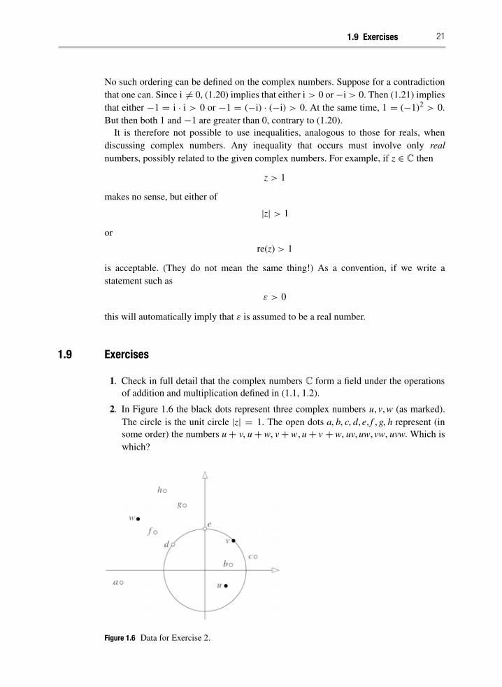
2. In Figure 1.6 the black dots represent three complex numbers u, v,w (as marked).
The circle is the unit circle |z| = 1. The open dots a, b, c, d, e, f ,g, h represent (insome order) the numbers u+ v, u+ w, v+ w,u+ v + w, uv,uw, vw, uvw. Which iswhich?
Figure 1.6 Data for Exercise 2.

22 Algebra of the Complex Plane
3. By writing z in the form z = a+ bi, find all solutions z of the following equations:(i) z2 = −5+ 12i
(ii) z2 = 2+ i
(iii) (7+ 24i)z = 375
(iv) z2 − (3+ i)z+ (2+ 2i) = 0
(v) z2 − 3z+ 1+ i = 0
4. If λ is a positive real number, show that
{z ∈ C : |z| = λ|z− 1|}
is a circle, unless λ takes one particular value (which?)5. Draw the set of points
{z ∈ C : re(z + 1) = |z− 1|}
by substituting z = x+ iy and computing the real equation relating x and y.
Now note that re(z+1) is the distance from z to the line y = −1, and |z−1| is thedistance between z and 1. Compare with the classical ‘focus-directrix’ definition ofa parabola: the locus of a point equidistant from a fixed line (here y = −1) and afixed point (here (x, y) = (1, 0)).
6. Draw the set of all z ∈ C satisfying the following conditions:(i) re(z) > 2
(ii) 1 < im(z) < 2
(iii) 1 < im(z− i) < 2
(iv) |z| < 2
(v) |z| > 1
(vi) 1 < |z| < 2
(vii) |z− 1| < 1
(viii) |z− 1| < |z + 1|
7. Draw the set of all z ∈ C satisfying the following conditions:(i) zz = 1
(ii) z+ iz+ 1+ i = 0
(iii) z+ z+ 2 = 0
(iv) z+ z+ 2i = 0
8. Let r, s, θ ,φ be real. Let
z = r(cos θ + i sin θ)w = s(cos φ + i sinφ)
Form the product zw and use the standard formulas for cos(θ + φ), sin(θ + φ) toshow that arg(zw) = arg(z) + arg(w) (for any values of arg on the right, and some
value of arg on the left).By induction on n, derive De Moivre’s Theorem
(cos θ + i sin θ)n = cos nθ + i sin nθ
for all natural numbers n.

1.9 Exercises 23
Figure 1.7 Data for Exercise 10.
Specialise to the case n= 3 and recover the usual formulas for cos 3θ and sin 3θin terms of cosθ and sin θ .
9. Use De Moivre’s Theorem (Exercise 8) and the substitution z = r(cos θ + i sin θ) toshow that the equation z3 = 1 has three distinct complex roots. Find them.Compute the square roots of 1 + i
√3,√3− i, and 1 + i, and the cube roots of√
3+ i, 1 − i, i. Sketch these points in the complex plane.10. In earlier textbooks, multiplication of complex numbers is often defined as follows.
Given two complex numbers z1 , z2 , represent them by points A and B in the complexplane; and let O, U be the points z = 0, 1 respectively, Figure 1.7.Draw triangle OBC similar to triangle OUA (where ∠BOC = ∠UOA, ∠OBC =
∠OUA). Then z1z2 is represented by the point C so constructed.Using the fact that |z1z2| = |z1||z2|, and the result of Exercise 5, show that this
construction agrees with our definition (1.2).11. Define a square root
√z of a complex number z to be any complex number w such
that w2 = z. Prove that every non-zero complex number has exactly two squareroots, and give formulas for them in terms of re z and im z.
If a,b, c ∈ Cwith a ²= 0, show that the solutions of the quadratic equation
az2 + bz+ c = 0
are precisely
z = −b³√b2 − 4ac2a
12. Use De Moivre’s Theorem (Exercise 8) to compute cos 5θ and sin 5θ in terms ofcos θ and sin θ .
13. Prove that De Moivre’s Theorem remains true if n is a negative integer.14. Define a kth root k
√z to be any w such that wk = z. Use De Moivre’s Theorem to
find an expression for k√r(cos θ + i sin θ).

2 Topology of the Complex Plane
In this chapter we collect together the basic topological ideas required for our study ofcomplex analysis. The list is not very demanding. Some items are needed to handle dif-ferentiation neatly, and some are needed for integration. Differentiation is naturally setagainst a background of limits and continuity, and these are best dealt with on open sets.On the other hand, an interval from one complex number to another is computed alonga specified path between them. A set in which any two points can be joined by a path issaid to be path-connected. To be able to cope with both integration and differentiationin the simplest possible manner later on, we restrict our complex functions to be thosedefined on open path-connected sets. Such a set is called a domain.
When the set is open we often abbreviate ‘path-connected’ to ‘connected’. The term‘connected’ is used in point-set topology with a specific technical meaning, but foropen sets in C it is equivalent to being path-connected. So this abbreviation does noharm.
Domains can have exotic shapes and paths can wiggle around a great deal. To beable to appeal to geometric intuition without our imagination having to work over-time thinking about such complications, we use a carefully conceived technical devicecalled the Paving Lemma. We show in this lemma that a path in an open set (in par-ticular, a domain) can be subdivided into a finite number of smaller pieces in sucha way that each piece is contained in a disc within the open set, thus ‘paving’ thepath with discs, see Figure 2.1. A disc is the interior of a circle, which is geomet-
rically very simple: for instance, any two points in it can be joined by a straightline. Joining the end points of pieces of the original path in each disc paving it, weobtain a new path made up of straight line segments, still lying in the open set andjoining the ends of the original path. We see, therefore, that given any path what-soever between two points in an open set, no matter how much the path twists andturns, there is an alternative path in the open set, between the same points, that ismade up of a finite number of straight line segments. We can even insist that the seg-ments are parallel to the real or imaginary axis, giving a step path in the open set. Todo so, take a suitable step path inside each paving disc and join them together, seeFigure 2.2.With techniques such as this we can use the Paving Lemma to illuminate complex
analysis, yielding fully rigorous proofs linked firmly to geometric intuition.

Topology of the Complex Plane 25
Figure 2.1 A domain (shaded) and a path in the domain (solid curve). Circles show a finite set ofdiscs inside the domain, whose union contains the path.
Figure 2.2 Replacing the path in Figure 2.1 by a step path.

26 Topology of the Complex Plane
2.1 Open and Closed Sets
DEFIN IT ION 2.1. For a complex number z0 and a positive real number ε, theε-neighbourhood of z0 is
Nε(z0) = {z ∈ C : |z− z0| < ε}
This is an open disc of radius ε.Geometrically, Nε(z0) is the disc centre z0 of radius ε, Figure 2.3.A subset S ⊆ C is said to be open if for every z0 ∈ S there is a real number ε such
that Nε(z0) ⊆ S. We emphasise that ε may depend on z0.
Example 2.2. The disc Nε(z0) is itself open, for if z1 ∈ Nε(z0) then |z1 − z0| < ε.Choose δ > 0 such that δ < ε − |z1 − z0|. By the triangle inequality, Nδ (z1) ⊆ Nε(z0),
Figure 2.4.
DEFIN IT ION 2.3. The complement of a subset S ⊆ C is
C \ S = {z ∈ C : z /∈ S}
A subset S is closed if C \ S is open.
Figure 2.3 The ε-neighbourhood of a point z0 .
Figure 2.4 The ε-neighbourhood of z0 is open.

2.2 Limits of Functions 27
There is another way to characterise closed sets, using the notion of a limit point ofa subset S. A complex number z0 is a limit point of S if every neighbourhood Nε(z0)
contains a point of S not equal to z0 . In this definition, z0 does not itself have to belongto S, though it may do. The essential feature of a limit point of S is that it has points ofS arbitrarily close to it. In fact, each Nε(z0) must contain an infinite number of points ofS – for if some Nε(z0) contains only finitely many points z1, . . . , zn of S, distinct fromz0 , we can take ε1 to be the smallest of the distances |z0 − zr|. Then Nε1(z0) contains nopoints of S, a contradiction.An alternative characterisation of a closed set is:
PROPOSIT ION 2.4. A subset S ⊆ C is closed if and only if S contains all its limitpoints.
Proof. Suppose S is closed and z0 is a limit point. If z0 ∈ C \ S, which is open, thenNε (z0) ⊆ C \ S for some ε > 0, so Nε (z0) contains no point of S, contradicting z0 being
a limit point. Hence z0 ∈ S.
Conversely, suppose that S contains all its limit points. Then any z0 ∈ C \ S is not alimit point of S, so there exists ε > 0 such that Nε(z0) contains no point of S. ThereforeNε (z0) ⊆ C \ S, so C \ S is open, and S is closed.
Not every point of a closed set need be a limit point of that set. For instance, if
T = {z ∈ C : z = 0 or z = 1/n for a positive integer n}
then the only limit point of T is 0. Since this is in T , the set T is closed.Points in S that are not limit points of S are said to be isolated points of S. All points
of T except 0 are isolated points of T.In general, an isolated point z0 of S has a neighbourhood Nε(z0) that contains no points
of S other than z0 . For instance, in the set T , if ε = 1n− 1
n+1then Nε (1/n) contains no
other points of T. On the other hand, it is clear from the definitions that every element
of an open set is a limit point of that set.We will also need:
DEFIN IT ION 2.5. The closure of a subset S ⊆ C is the intersection of all closed subsetsthat contain S. This is closed, and is the smallest closed subset containing S. It consistsof S together with all limit points of S.
2.2 Limits of Functions
The notion of a limit
limz→z0
f (z)
is analogous to the real case, and its properties follow by similar arguments.
DEFIN IT ION 2.6. If f : S→ C is an arbitrary complex function and z0 is a limit pointof S, then limz→z0 f (z) = l if, given any ε > 0, there exists δ > 0 such that
for all z ∈ S, 0 < |z− z0| < δ implies | f (z) − l| < ε (2.1)

28 Topology of the Complex Plane
Two points should be made about this definition:(a) The point z0 need not belong to S, so f (z0) need not be defined. Even if z0 ∈ S,
f (z0) may not equal l.For example, if
f (z) =
±0 (z ±= 0)
1 (z = 0)
then limz→0 f (z) = 0 ±= f (0)
(b) It is essential that z0 is a limit point of S, or else there would exist δ > 0 such that{z : |z− z0| < δ} contains no point of S. In this case condition (2.1) would be vacuouslytrue for any l ∈ C.As in the real case, we have:
PROPOSIT ION 2.7. If z0 is a limit point of S and limz→z0 f (z) = l, the limit is unique.
Proof. Suppose that l² ±= l is another candidate for the limit. Take ε = 12|l − l²| to find
δ1 > 0,δ2 > 0 such that
z ∈ S, 0 < |z− z0| implies | f (z)− l| < εz ∈ S, 0 < |z− z0| implies | f (z)− l²| < ε
Because z0 is a limit point, there exists z∗ ∈ S, where 0 < |z0 − z∗| < min(δ1, δ2). Then
|l− l²| = |l− f (z
∗)+ f (z
∗)− l
²|
≤ |l− f (z∗)| + | f (z∗) − l²|
< ε + ε
= 2ε
contradicting the choice of ε.
Standard properties of complex limits may be proved using methods analogous to thereal case:
PROPOSIT ION 2.8. If limz→z0 f (z) = l, limz→z0 g(z) = k, then
(i) limz→z0 f (z)+ g(z) = l+ k
(ii) limz→z0 f (z)− g(z) = l− k
(iii) limz→z0 f (z)g(z) = lk
(iv) limz→z0 f (z)/g(z) = l/k (for l ±= 0)
Proof. Part (i) is routine. Part (ii) follows immediately if we first show that
limz→z0(−g(z)) = −k, which is trivial.Part (iii) is a little trickier. Bear in mind that f (z0),g(z0) may not be defined since z0
need not belong to S. Write
| f (z)g(z)− lk| = | f (z)g(z) − lg(z)+ lg(z)− lk| (2.2)
≤ | f (z)− l||g(z)| + |l||g(z)− k| (2.3)

2.2 Limits of Functions 29
Since limz→z0 g(z) = k, there exists δ0 > 0 such that
z ∈ S and 0 < |z− z0| < δ implies |g(z) − k| < ε
Therefore |g(z)| < |k| + ε = M, say, whenever 0 < |z− z0|. Therefore |g(z)| is boundedabove near (but not necessarily at) z0 byM.
Since limz→z0 f (z) = l, there exists δ1 > 0 such that
z ∈ S and 0 < |z− z0| < δ1 implies | f (z) − l| < ε/(2M)
Let N ∈ R such that N > |l|, so in particular N > 0. Since limz→z0 g(z) = k, there existsδ2 > 0 such that
z ∈ S and 0 < |z− z0| < δ2 implies |g(z) − k| < ε/(2N)
For δ = min(δ0, δ1 , δ2) we then have
z ∈ S and 0 < |z − z0| < δ1 implies
| f (z) − l||g(z)| + |l||g(z)− k| <ε
2MM+ N
ε
2N= ε
By (2.3), for z ∈ S and 0 < |z− z0| < δ2, we have
| f (z)g(z) − lk| < ε
proving (iii).To prove (iv), it is enough to prove that limz→z0 1/g(z) = 1/k, and then to appeal to
(iii) for the functions f , 1/g.For this to make sense we must show that for some δ1 > 0, g(z) is not zero when
z ∈ S and 0 < |z− z0| < δ1 . Then 1/g(z) is defined.This follows since limz→z0 g(z) = k and k ±= 0. Indeed, there exists δ1 such that
z ∈ S and 0 < |z− z0| < δ1 implies |g(z) − k| < 12 |k|
which in turn tells us that
z ∈ S and 0 < |z − z0| < δ1 implies |g(z)| > 12|k|
We now find δ2 such that
z ∈ S and 0 < |z− z0| < δ2 implies |g(z) − k| < 12|k|
2ε
Now, if δ = min(δ1, δ2),
z ∈ S and 0 < |z − z0| < δ implies²²²²
1
g(z)−
1
k
²²²²<|k − g(z)|
|g(z)k|< 1
2 |k|2ε/( 12 |k|
2) = ε
The real and imaginary parts of a complex function,
f (z) = re f (z) + i im f (z)
may be considered separately. If
limz→z0
f (z) = l = α + iβ (α, β ∈ R) (2.4)

30 Topology of the Complex Plane
then, because
|re f (z) − α| = |re( f (z) − l)| ≤ |( f (z)− l)|
we deduce from the definition that
limz→z0
re f (z) = α (2.5)
Proposition 2.8 (ii) now implies that
limz→z0
im f (z) = β (2.6)
Conversely, if (2.5,2.6) both hold, Proposition 2.8 (i) implies (2.5).We can rephrase the preceding argument by recalling that if S ⊆ R2 the limit of a real
function φ : S→ R of two variables, φ(x, y) for (x, y) ∈ S is defined as follows:
φ(x, y)→ λ as (x, y) → (a, b) if, given ε > 0, there exists δ > 0 such that
for all (x, y) ∈ S, 0 <³(x− a)2 + (y− b)2 < δ implies |φ(x, y)− λ| < ε
Identifying (x, y) with z = x+ iy ∈ C, and setting z0 = a+ ib, this may be written as
z ∈ S and 0 < |z− z0| < δ implies |φ(x, y) − λ| < ε
If we now write
f (z) = u(x, y) + iv(x, y)
where the real and imaginary parts of f are considered as real functions u and v of tworeal variables x, y, we have proved:
PROPOSIT ION 2.9. Let z0 = a+ ib. Then limz→z0 f (z) = l = α + iβ if and only if
u(x, y)→ α v(x, y)→ β as (x, y)→ (a,b)
In this way, the limit of a complex functions is equivalent to the limit of a pair of realfunctions of two real variables. However, the notation in the complex case is generallysimpler.
2.3 Continuity
The definition of continuity for a complex function mimics that for a real function, usingthe complex version of the modulus:
DEFIN IT ION 2.10. A function f : S→ C is continuous at z0 ∈ S if, given ε > 0, thereexists δ > 0 such that
for all z ∈ S, |z− z0| < δ implies | f (z)− f (z0)| < ε
A function is continuous if it is continuous at every point z0 ∈ S.

2.3 Continuity 31
If z0 is a limit point of S, this is equivalent to saying that limz→z0 f (z) exists and
limz→z0
f (z) = f (z0)
If z0 is an isolated point of S then there is a neighbourhood Nδ(z0) that contains noother points of S apart from z0, so
for all z ∈ S, |z − z0| < δ implies z = z0
which in turn implies
| f (z)− f (z0)| = 0
So a complex function is always continuous at an isolated point, according to the defi-nition. Actually, this will not be an issue for us, because we will consider only functionswhere all points of S are limit points. In fact, S is usually open. But it seemed worthtidying up a potential loose end.We can rephrase the definition of continuity in terms of open discs: f is continuous at
z0 ∈ S if, given ε > 0, there exists δ > 0 such that
for all z ∈ S, z ∈ Nδ(z0) implies f (z) ∈ Nε ( f (z0))
Or, more succinctly,
f (Nδ(z0)) ⊆ Nε( f (z0))
We can develop an alternative way to define continuous functions in terms of opensets. First we need a generalisation: a subset V ⊆ S is said to be relatively open in S, orjust open in S for short, if for every z0 ∈ V there exists σ > 0 such that Nσ (z0)∩ S ⊆ V .
Example 2.11. A relatively open set need not be open. The interval (a,b) = {x ∈ R :
a < x < b} is open in R, but not in C. In fact, when S = C let x ∈ (a,b) andsuppose that σ > 0. Then x + iσ/2 ∈ Nσ (x) = Nσ (x) ∩ S, but x + iσ/2 ±∈ V . SeeFigure 2.5.
Figure 2.5 The interval (a, b) is open in R but not in C.

32 Topology of the Complex Plane
Using the standard set-theoretic notation
f−1(U) = {z ∈ S : f (z) ∈ U}
we get an alternative characterisation of a continuous function:
PROPOSIT ION 2.12. A complex function f : S → C is continuous if and only if, forevery open set U in C, the set f−1(U) is open in S.
Proof. Suppose that f is continuous and U is open. Let z0 ∈ f −1(U). Then f (z0) ∈ U so
there exists ε > 0 such that Nε( f (z0)) ⊆ U. By continuity of f there exists δ > 0 suchthat
f (Nδ(z0)∩ S) ⊆ Nε( f (z0)) ⊆ U
Hence
Nδ(z0)∩ S ⊆ f−1(U)
and f−1(U) is open.Conversely, suppose that f −1(U) is open in S for every open set U. Given z0 ∈ S and
ε > 0, the set Nε( f (z0)) is open, so f−1(Nε( f (z0))) is open in S and there exists δ > 0
such that
Nδ(z0)∩ S ⊆ f−1(Nε( f (z0)))
Hence
f (Nδ(z0)∩ S) ⊆ Nε( f (z0))
so f is continuous.
Proposition 2.12 is favoured by topologists as the definition of continuity. It is partic-ularly useful when S is itself an open set. Then, given a subset V ⊆ S that is open in S,and any z0 ∈ V, there exist σ , ε > 0 such that
Nσ (z0) ⊆ V (because V is open in S)Nε(z0) ⊆ S (because S is open)
Taking δ = min(ε, σ ), we deduce that
Nδ(z0) ⊆ V
so V is an open set in C. This proves:
COROLLARY 2.13. If S ⊆ C is open, then f : S → C is continuous if and only if, forevery open set U, the inverse image f −1(U) is open.
Figure 2.6 illustrates this result.Composition of two functions is defined in the usual manner: if f : S → C and
g : T → C where f (S) ⊆ T, then g ◦ f : S→ C is given by
g ◦ f (z) = g( f (z))

2.3 Continuity 33
Figure 2.6 Definition of continuity when S is open in C.
PROPOSIT ION 2.14. If f is continuous at z0 ∈ S and g is continuous at f (z0), then g ◦ fis continuous at z0 .
Proof. Easy exercise.
Addition, subtraction, multiplication, and division of complex functions f1 : S → C
and f2 : S→ C are defined by
f1 + f2 : S→ C where ( f1 + f2)(z) = f1(z)+ f2(z) (z ∈ S)
f1 − f2 : S→ C where ( f1 − f2)(z) = f1(z)− f2(z) (z ∈ S)
f1f2 : S→ C where ( f1f2)(z) = f1(z)f2(z) (z ∈ S)
f1/f2 : S→ C where ( f1/f2)(z) = f1(z)/f2(z) (z ∈ S²)
Here S² = {z ∈ S : f2(z) ±= 0}.
Warning: the composition g ◦ f is often abbreviated to g f when it is clear that theproduct is not intended.
PROPOSIT ION 2.15. If f1 and f2 are continuous, then so are f1 + f2 , f1 − f2, f1 f2 , andf1/f2 (when f2(z) ±= 0).
Proof. This is a direct consequence of Proposition 2.8.
This result lets us show very quickly that certain functions built up from functionsknown to be continuous are themselves continuous. For instance, the constant functionk(z) = c (where c ∈ C) and the identity function I(z) = z are clearly continuous. We
give the easy proofs. Let ε > 0. For k take any δ > 0; then
|z− z0| < δ implies |k(z)− k(z0)| = |c− c| = 0 < ε
For I take δ = ε; then
|z− z0| < ε implies |I(z) − I(z0)| = |z− z0| < ε

34 Topology of the Complex Plane
On that basis, Proposition 2.15 shows immediately that f (z) = cz is continuous. Byinduction on n, it follows that f (z) = czn is continuous for any n ∈ N. A further inductionproves that any polynomial function
f (z) = anzn + an−1z
n−1 + · · · + a0
is continuous. Then any rational function p(z)/q(z), where p,q are polynomials, is con-tinuous at any point z0 where q(z0) ±= 0. Using these ideas we seldom have to performany intricate epsilon-delta calculations.
Example 2.16. The modulus function m(z) = |z| is continuous for all z. Given ε > 0,
take δ = ε. Then
|m(z)− m(z0)| < ε implies ||z| − |z0|| ≤ |z− z0| < ε
using (1.12).
Example 2.17. f (z) = |z|2+17z3+1066z1+z is continuous for z ±= −1. Proving this with an
explicit choice of δ for given ε is tedious and messy. A quicker way is to observe that|z|2 = |z||z| and is therefore continuous, 17z3 + 1066z is a polynomial and so is alsocontinuous, and the same goes for z + 1. Since we are dividing by this, we must havez ±= −1.
Writing f (z) = u(x, y)+iv(x, y) for z = x+ iy ∈ S, where u, v are real-valued functionsof the real variables x, y, Proposition 2.9 gives:
PROPOSIT ION 2.18. The function f (z) = u(x, y)+iv(x, y) is continuous at z0 = x0+iy0if and only if u, v are continuous at (x0 , y0).
Example 2.19. If f (z) = z2 , then f (z) = (x+iy)2 = x2−y2+2ixy. Hence u(x, y) = x2−y2
and v(x, y) = 2xy. The function f is continuous for all z ∈ C, just as u, v are continuousfunctions of x, y for all (x, y) ∈ R2 .
An interesting case occurs when S is the real interval
S = [a,b] = {x ∈ R : a ≤ x ≤ b}
considered as a subset of C. Here z = x + 0i, so we can simplify notation and writef (z) = u(x)+ iv(x). Now the function f : [a,b]→ C is continuous if and only if both uand v are continuous.
Example 2.20. f : [0, 1]→ C, where f (x) = x2+ ix3 is continuous, since both u(x) = x2
and v(x) = x3 are continuous.
Functions defined on a real interval play a central role because they define paths, aswe now discuss.

2.4 Paths 35
2.4 Paths
In the early development of complex analysis, mathematicians worked out how to inte-grate complex functions along paths inC, without worrying too much about the meaning
of ‘path’. This happened back in the days when notions of continuity and limits werestill under development. The intuitive idea of a path (or curve) was something that couldbe drawn by moving a pencil (with an infinitely fine point) without making any jumps.
Such paths were assumed to have various nice properties, such as having a continuouslyvarying tangent, or not crossing themselves. These properties were not made explicituntil the foundational issues in analysis were sorted out, in particular by Bolzano andWeierstrass.
Later it turned out that some of these assumptions are not necessary to develop asatisfactory theory of integration, while others must be made precise to avoid runninginto contradictions. We have no wish to make readers repeat all the twists and turns ofhistory; as we have said, some battles have already been won. But from time to time
we find it useful to point out some of the pitfalls that can arise, and to emphasise some
subtle distinctions – for example, the definition of a path as a map γ from a real interval[a,b] into the complex plane, and the distinction between this map and its image. Ourpictures generally show the image, leaving the reader to infer the map. We often add anarrow as a reminder that as a parameter t runs through the interval [a,b], the point γ (t)moves along the image in a specific direction.One of the pleasant features of complex analysis is that fairly often that information
is all we need. At various points in the book we also find it useful to impose furtherconditions on paths, to ensure that they have appropriate properties.The upshot of more than a century of deep contemplation and debate is the following
definition:
DEFIN IT ION 2.21. A path in the complex plane is a continuous function
γ : [a, b] →C (a ≤ b ∈ R)
Its initial point is γ (a) and its final point (or end point) is γ (b).
Sometimes we speak of γ as ‘a path in C from z1 to z2’ when z1 = γ (a) is the initialpoint and z2 = γ (b) is the final point. When t ∈ [a, b] we also refer to z = γ (t) as a‘point on the path γ ’, although strictly speaking z is on the image of the function γ . Ifwe think of t as ‘time’ and imagine t increasing from a to b, the point γ (t) traces a curvein the plane from γ (a) to γ (b). When drawing a diagram we often indicate the directionof motion (increasing t) by an arrow, as in Figure 2.7. However, it must be emphasised
that this is a makeshift device since the curve may cross itself or turn back on itself, sothe picture may get quite complicated. We pick up this point again in Section 6.7.
2.4.1 Standard Paths
To simplify matters, when we speak of line segments and circles, considered as paths,we assume they are specified by the following standard functions:

36 Topology of the Complex Plane
Figure 2.7 A path in C, showing its parametrisation by t ∈ [a, b].
(i) The line segment L = [z1, z2] from z1 to z2 is
L(t) = (1− t)z1 + tz2 (t ∈ [0, 1])
When z1 = a, z2 = b ∈ R then the image of the path is the closed interval [a, b] ⊆R ⊆ C.
(ii) The unit circle C:
C(t) = cos t + i sin t (t ∈ [0, 2π ])
(iii) The circle S with centre z0 and radius r ≥ 0:
S(t) = z0 + r(cos t + i sin t) (t ∈ [0, 2π ])
See Figure 2.8.
Figure 2.8 Three standard paths.

2.4 Paths 37
Figure 2.9 ‘Graphs’ of paths considered as functions [a, b]→ C. Left: A path that travels oncealong the image in a fixed direction. Right: A path that travels once along the image, turns roundand travels back, then turns again and travels along the image for a third time.
2.4.2 Visualising Paths
We are used to visualising a function f : R→ R using the corresponding graph y = f (x)
in the plane. A similar idea can be exploited to visualise paths in a more explicit way.Figure 2.9 shows analogues of graphs for two maps γ : [a,b] → C. The arrows joinrepresentative points t ∈ [a,b] to their images γ (t) ∈ C. The left-hand figure illustratesa path where γ (t) travels along the image without turning back on itself. The right-handfigure illustrates a path where γ (t) travels along the image to the far end, turns back onitself to revisit the start, then turns back again to travel along the image for a third time.Although paths like this are seldom encountered in practice, they are allowed by thedefinition, so we have to take that possibility into account. Example 6.17 below showsthat simple formulas can produce this type of behaviour.An alternative would be to change the definition to rule out such behaviour, but most
of the theory works in the general case with no extra effort, so it turns out to be simplerto leave the definition as it stands, while bearing in mind that simple pictures might bemisleading in some respects.
2.4.3 The Image of a Path
To emphasise the distinction between a path and its image we introduce a furtherdefinition:
DEFIN IT ION 2.22. A curve C from z1 to z2 in the complex plane is a subset of C thatis equal to the image of a path γ : [a, b]→ C, where γ (a) = z1 and γ (b) = z2.
Given a curve C, a parametrisation of C is a path σ : [c, d]→ C such that C is theimage of σ , where σ (a) = z1 and σ (b) = z2.
The corresponding parameter is a variable t ∈ [a, b].We sometimes call [a, b] the parametric interval of σ .

38 Topology of the Complex Plane
Figure 2.10 The two distinct paths γ1 ,γ2 have the same image, so they define the same curve.
If we think of t as ‘time’, and imagine a particular parametrisation γ : [a,b] → C,
then as t increases from a to b the point γ (t) traces the corresponding curve in the planefrom γ (a) to γ (b), moving continuously with t.
Example 2.23. The same curve may be traced by many different paths. For example, inFigure 2.10 the paths
γ1(t) = 2(t + it) (0 ≤ t ≤ 12 )
γ2(t) = t2 + it2 (0 ≤ t ≤ 1)
traverse the same curve
{x+ iy ∈ C : x = y, 0 ≤ x ≤ 1}
2.5 Change of Parameter
Definition 2.21 equips every path γ : [a,b]→ C with a parameter t ∈ [a,b]. It is oftenconvenient to change the parameter and its parametric interval, because suitable choicescan simplify calculations and proofs. In this section we discuss such changes.We begin with Example 2.23, which distinguishes a path from its image by exhibiting
two different paths that have the same image curve. Dynamically, these two paths tracethe same curve in the same direction, but at different speeds. They are related by thechange of parameter ρ : [0, 12] → [0, 1], where ρ(t) = 1
2 t2 . This has an inverse map
ρ−1 : [0, 1]→ [0, 1
2] given by ρ−1(s) =
√2s.
We now discuss general changes of parameter, defined as follows:
DEFIN IT ION 2.24. Let γ : [a, b] → C be a path, and suppose that ρ : [c,d] → [a,b]
is continuous and satisfiesρ(c) = a ρ (d) = b

2.6 Subpaths and Sums of Paths 39
so in particular ρ is onto [a, b]. Then the composition γ ◦ ρ : [c,d]→ C is also a path.We call γ ◦ ρ a reparametrisation of γ .
Note that the parametric interval changes when [c,d] ±= [a,b].
2.5.1 Preserving Direction
If we impose extra conditions on ρ, a change of parameter can preserve extra properties.The image of the path is important, but another property is also vital: the direction inwhich the path is traced. Now our mental image involves the dynamics of a point moving
along the path, as well as the image that it traces out.At this stage we are working with general continuous paths, so we adopt the fol-
lowing approach. Recall that a map σ : [a,b] → [c,d] is strictly increasing if
a ≤ t1 < t2 ≤ b implies σ (t1) < σ (t2). Both of the above maps ρ and ρ−1 are strictlyincreasing.
In real analysis it is proved that any strictly increasing continuous map has a strictlyincreasing continuous inverse. We give the easy proof for completeness:
LEMMA 2.25. If ρ : [a, b] → [c, d] is continuous and strictly increasing with ρ(a) = c
and ρ(b) = d, then ρ has a strictly increasing continuous inverse ρ−1 : [c,d]→ [a,b].
Proof. If s ∈ [c, d] then ρ(a) ≤ s ≤ ρ(b). By the Mean Value Theorem there existst ∈ [a,b] such that ρ(t) = s. This determines a strictly increasing inverse functionρ−1 : [c,d] → [a, b], where ρ and ρ−1 both map open intervals to open intervals, soρ−1 is also continuous.
We can now state:
DEFIN IT ION 2.26. Let C be a curve, parametrised by two maps γ : [a,b] → C and
λ : [c,d] → C. The maps have the same direction if there is a strictly increasing functionρ : [a,b]→ [c,d] such that
γ = λ ◦ ρ
Then ρ is a direction preserving change of parameter.
If the change in parameter ρ is not increasing, it can lead to part of the curve beingtraced back and forth as t increases. In Figure 2.11, as t increases from p to q, the valueof ρ(t) increases, then decreases, then increases again. As this happens, the points onthe curve from P to Q are traversed first in the direction from P to Q, then back to P,then from P to Q once more. The curve is the same, but the distance travelled increases.This means that when we calculate the length of a curve, defined in Section 6.3, we must
prescribe how the curve is traced.
2.6 Subpaths and Sums of Paths
In the general theory, and in applications, it is useful to be able to chop paths into pieces,or join pieces together.

40 Topology of the Complex Plane
z-plane
c d
a t b
ρ(t) changes direction
as t increased from p to qρ
γ
ρ(t)a t b
c
d
ρ(t)
p q
image(γρ)
z= γ(ρ(t))
p
Q
Figure 2.11 Left: A change in parameter. Right: If ρ has a graph like this then the parameter t
changes direction along the image curve.
DEFIN IT ION 2.27. For an arbitrary path γ : [a,b] → C, a subpath is obtained byrestricting γ to a subinterval [c,d], where a≤ c ≤ d ≤ b. If
a= x0 < x1 < · · · < xn = b
and γr is the subpath obtained by restricting γ to [xr−1 , xr], we write
γ = γ1 + · · · + γn
In so doing, we think of γ as being made up by tracing along the paths γ1 , . . . , γn taken
in order, see Figure 2.12.
Figure 2.12 Decomposing a path into subpaths.
Similarly, if the final point of a path γ1 coincides with the initial point of a path γ2 ,it is useful on occasion to create a combined path by first tracing γ1 and then γ2. Thereis a minor technicality here, because γ1(b) can be the same as γ2(c) even though γ1 is
defined on [a,b] and γ2 defined on [c,d] where b ±= c. The next example shows how toget round this difficulty.

2.6 Subpaths and Sums of Paths 41
Figure 2.13 Joining two paths by shifting parameters.
Example 2.28. Suppose that
γ1(t) = t (t ∈ [0, 1])γ2(t) = cos t + i sin t (t ∈ [0,π])
as in Figure 2.13. Here γ1(1) = γ2(0) but 1 ±= 0.
In such a case we extend our notation a little. Suppose that γ1 : [a,b] → C, andγ2 : [c,d] → C, with γ1(b) = γ2(c). Then we define the combination γ = γ1 + γ2 :
[a,b+ d − c]→ C by
γ (t) =
±γ1(t) (t ∈ [a,b])
γ2(t + c− b) (t ∈ [b,b+ d− c])
In effect, what we have done is to shift the parametric interval of the second path from[c,d] to [b,b+ d − c], by adding b− c to all points in [c, d].In Example 2.28, for instance,
γ (t) =
±t (t ∈ [0, 1])cos(t− 1)+ i sin(t− 1) (t ∈ [1, 1+ π])
and γ consists of the line segment γ1 followed by the semicircle γ2.
The path γ1 + γ2 is defined only when the final point of γ1 is the same as the initialpoint of γ2, so perhaps this is not a fully appropriate use of the + sign. However, we dohave
(γ1+ γ2)+ γ3 = γ1 + (γ2 + γ3) (2.7)
whenever the appropriate end points coincide, so we can omit the parentheses in such a‘sum’, and more generally write γ1 + · · · + γn to indicate the path obtained by succes-sively tracing γ1, . . . ,γn, whenever the final point of each γr−1 coincides with the initialpoint of γr(1 ≤ r ≤ n).

42 Topology of the Complex Plane
Equation (2.7) states that addition of paths is associative, but in general it is not com-
mutative. Exercises 7 and 8 provide simple examples to show that when γ1 + γ2 is
defined, γ2 + γ1 may not be, and even when it is, γ1 + γ2 need not equal γ2 + γ1.
For a path γ : [a,b]→ C, another useful concept is the opposite path −γ : [a, b] →C defined by
−γ (t) = γ (a+ b− t) (t ∈ [a,b])
As t increases from a to b, so −γ describes the same curve as γ , but it does so in thereverse direction. If γ is a path from z1 to z2, then −γ is a path from z2 to z1 .
Example 2.29. Suppose that L is the line segment [z1, z2] given by
L(t) = (1 − t)z1 + tz2 (t ∈ [0, 1])
Then −L is given by
−L(t) = tz1+ (1− t)z2 (t ∈ [0, 1])
which is, of course, [z2, z1].If S is the circle centre z0 and radius r ≥ 0, then
S(t) = r(cos t + i sin t) (t ∈ [0, 2π ])
describes the circle once, anticlockwise, while the opposite path
−S(t) = z0 + r(cos(2π − t) + i sin(2π − t)) (t ∈ [0, 2π ])= z0 + r(cos t − i sin t) (t ∈ [0, 2π ])
describes it once, clockwise.
In a sum such as γ1 + (−γ2) + γ3 we omit the parentheses and write γ1 − γ2+ γ3 .
This is the path that traces first along γ1, then back along the opposite path to γ2 ,
and then along γ3. As always, the appropriate final and initial points must agree. SeeFigure 2.14.
Figure 2.14 The path γ1 − γ2 + γ3.

2.7 The Paving Lemma 43
Figure 2.15 The pathCR + L1 − Cε + L2.
Example 2.30. Suppose that 0 < ε < R and
CR(t) = R(cos t + i sin t) (t ∈ [0,π ])
Cε (t) = ε(cos t + i sin t) (t ∈ [0,π ])
L1(t) = t (t ∈ [−R,−ε])
L2(t) = t (t ∈ [ε, R])
Then CR +L1− Cε +L2 is the path describing the curve in Figure 2.15 once, anticlock-wise.
2.7 The Paving Lemma
We now come to a technical lemma that plays a vital role in our approach to complex
integration, which we call the Paving Lemma. This result is so important that we presenttwo different proofs of it. To set it up, we first need another piece of terminology.
A path γ : [a,b]→ C is said to be a path in S if the image
{γ (t) : t ∈ [a,b]} ⊆ S
We signify this by writing γ : [a,b]→ S.
Example 2.31. The unit circle C(t) = cos t + i sin t (t ∈ [0, 2π]) is a path in the regionS = {z ∈ C :
12 ≤ |z| ≤ 2}, Figure 2.16.
A region of this form, contained between two concentric circles, is called an annulus.
This example is very simple. It must not lull us into a false sense of security: far more
intricate paths are possible.

44 Topology of the Complex Plane
Figure 2.16 Path in an annulus.
Figure 2.17 A more complicated path.
Example 2.32. Let V = {z ∈ C : z ±= 1/n for a non-zero integer n} and define
σ (t) =
±t + it cos(π/t) (t ∈ [−1, 1] \ {0})0 (t = 0)
Then σ is a path in V , Figure 2.17. Here σ winds in between the points 1/n where n is
a non-zero integer, crossing the real axis when t = 1/(n+ 12 ).
It does not take much imagination to realise that an open set S can be very compli-
cated, and a path γ can be intertwined in S in a very intricate manner. The space-fillingcurve described in Section 2.9 is given by a path whose image is the unit square, includ-ing its interior. Much more complicated images are possible. Rather than trying toimagine all possible intricacies, we sidestep the issue, as follows. If S is an open set,

2.7 The Paving Lemma 45
Figure 2.18 Paving a path with a sequence of discs. But could this process get stuck?
we can cover γ with a finite number of open discs, all contained in S. Then we use thediscs to simplify the path, as the next result explains.
LEMMA 2.33 (Paving Lemma). Let γ : [a, b] → S be a path in an open set S. Thenthere exists a subdivision a = t0 < t1 < · · · < tn = b such that each subpath γr
obtained by restricting γ to [tr−1, tr] lies inside an open disc Dr ⊆ S.
Proof. Because S is open, there is an open disc D1 such that γ (a) ∈ D1 ⊆ S.
The idea of the proof is that if the path has been paved up to some point, we canalways add another disc to take the paving further, unless we have reached the far end.Making this argument rigorous takes a little care, however, as we now indicate.The disc D1 is the first in a sequence of discs, obtained by moving along the path,
covering it bit by bit with discs as in Figure 2.18. The existence of D1 shows we can getstarted. Indeed, since γ is continuous, there exists δ > 0 such that
γ (t) ∈ D1 whenever a ≤ t < a+ δ (2.8)
Our only fear is that we might not progress all the way; for instance, the discs might
decrease dramatically in size and we might never reach the end. Some real analysisdispels this fear. If a ≤ x ≤ b, say that γ restricted to [a, x] ‘can be paved’ if it canbe subdivided into a finite number of subpaths γ1 , . . . ,γm, where each γr lies inside anopen disc Dr ⊆ S. Let P be the set of all x ∈ [a,b] such that [a, x] can be paved. We
know that a ∈ P so P is non-empty.
Also P is bounded above by b. Therefore, by real analysis, P has a least upper boundc, where a≤ c ≤ b. We claim that c = b, which will prove the lemma.
For a contradiction, suppose that c < b. Since S is open, there exists an open disc D
such that c ∈ D ⊆ S. By continuity of γ , there exists ε > 0 such that if c− ε < t < c+ε
and t ∈ [a, b], the image γ (t) ∈ D.
By (2.8), a + δ/2 ∈ P, so c > a. Since c is the least upper bound of P, there existsx ∈ Pwith c−ε < x < c. Therefore the segment {γ (t) : a ≤ t ≤ x} can be paved by open

46 Topology of the Complex Plane
discs D1 , . . . ,Dm all lying inside S. Let Dm+1 = D. Then the segment {γ (t) : a ≤ t ≤ c}
can be paved by open discs D1 , . . . ,Dm,Dm+1 all lying inside S.Finally, we claim that c = b. If c < b, continuity of γ implies that γ (c+ t) ∈ D for
all t such that 0 < t < τ , therefore [a, c+ τ/2] can be paved, contradicting c being anupper bound for P. Therefore c = b so [a, b] can be paved as required.
For future reference, and because this result is used repeatedly, we now give a secondproof, which in some respects is simpler. A generalisation to two dimensions will alsoprove useful in Proposition 9.5.
Alternative Proof of Lemma 2.33. We show more: the subdivision can be obtained byrepeatedly bisecting [a,b] a finite number of times. For the purposes of this proof only,it is useful to define and interval to be pavable if it can be bisected repeatedly a finitenumber of times into closed intervals, so that the image of every interval obtained in thismanner lies inside a disc in D. Otherwise, the interval is unpavable.Suppose the result is false. Then [a, b] is unpavable. Bisect [a,b] to get two closed
intervals, intersecting at the midpoint. At least one these intervals, call it I1 , is unpavable.Otherwise we could pave a finitely repeated bisection of each interval by finitely many
discs, whose union paves [a,b].Bisect I1. The same argument applies to the two halves, so we get an unpavable
closed interval I2 ⊆ I1 of half the size. Because we are assuming the result false, thissequence of bisections continues indefinitely to give a nested sequence of unpavableclosed intervals
[a,b] ⊇ I1 ⊇ I2 ⊇ · · ·
each half the size of the previous one.The intersection of these intervals is easily seen to be a unique point z0 ∈ D (Cauchy
sequences of real numbers converge). However, D is open, so there is a discNε (γ (z0)) ⊆
D. Since γ is continuous, γ−1(Nε (γ (z0))) is open in [a,b] and contains z0. Therefore itcontains In for sufficiently large n. Now In ⊆ Nε(γ (z0)), so it is pavable (with one disc),a contradiction.
In Example 2.31, for any point on the unit circle C, we have N1/2(z) ⊆ S. Clearly afinite number of such discs will pave C within S, Figure 2.19.However, the path in Example 2.32 cannot be paved by a finite number of discs in V .
Any disc containing the origin (which lies on σ includes points of the form 1/n lying
outside V . But this also means that V is not open. So the conditions required for thePaving Lemma are not satisfied.Readers familiar with basic point-set topology will recognise that the proof is ‘really’
about the compactness of the closed interval [a, b]. We prefer not to develop the abstractmachinery of compactness here; the Paving Lemma performs the same task.
2.8 Connectedness
We now define an important topological property, which is central to the theory ofcomplex functions.

2.8 Connectedness 47
Figure 2.19 Paving a circular path inside an annulus is easy.
Figure 2.20 A disc is path-connected.
DEFIN IT ION 2.34. A subset S ⊆ C is path-connected if, given z1 , z2 ∈ S, there existsa path γ in S from z1 to z2 .
Example 2.35. Any open disc Nr(z0) is path-connected. For, given z1 , z2 ∈ Nr(z0), letL(t) = (1− t)z1 + tz2, (t ∈ [0, 1]). Then
|L(t)− z0)| = |(1− t)z1 + tz2 − z0|
= |(1− t)z1 − (1− t)z0 + tz2 − tz0|
≤ (1− t)|z1 − z0| + t|z2 − z0|
< (1− t)r+ tr = r
so the line segment L lies in Nr(z0). See Figure 2.20.
Example 2.36. The set S = {z ∈ C : z = t + it2 , t ∈ R} is path-connected. For if t1+ it21and t2 + it22 ∈ S where t1 ≤ t2 , then γ (t) = t + it2 (t ∈ [t1 , t2]) is a path in S between
those points. See Figure 2.21.

48 Topology of the Complex Plane
Figure 2.21 The set {z ∈ C : z = t + it2 , t ∈ R} is path-connected.
Figure 2.22 A step path.
It is often convenient to use a very simple type of path.
DEFIN IT ION 2.37. A step path in S is a path γ : [a,b]→ S together with a subdivisiona = t0 < t1 < · · · < tn = b such that on each subinterval [tr−1 , tr] either re γ or im γis constant. This means that the image of γ consists of a finite number of straight linesegments, each parallel to the real or imaginary axis, see Figure 2.22.In other words, γ is a step path if γ = γ1 + · · · + γn where each γr is a line segment
parallel to the real or imaginary axis.A subset S ⊆ C is step-connected if, given z1 , z2 ∈ S, there exists a step path γ in S
from z1 to z2 .
Evidently a step-connected path is path-connected. The converse, however, is notalways true: Example 2.36 is path-connected but not step-connected. A path as simple asthe diagonal line segment [0, 1 + i] is path-connected but not step-connected. The main
issue here is that unlike a general continuous path, a step path consists of finitely many

2.8 Connectedness 49
straight line segments. But the requirement that these segments should be horizontal orvertical also comes into play.These considerations are mentioned here to help develop intuition, but they do not
cause problems for the theory, because every path-connected open set is step-connected.This constitutes the first success – albeit a minor one – for the Paving Lemma. To provethis, we first observe a simple fact:
LEMMA 2.38. Any open disc is step-connected.
Proof. Consider an open disc S = Nr(z0). Changing coordinates to z − z0 (translating
the origin) we may assume without loss of generality that z0 = 0. Let z1 = x1+ iy1 ∈ S.
We show that there is a step path in S from z1 to the centre 0. Let L1 be the (vertical)line segment from z1 to x1 , and L2 be the (horizontal) line segment from x1 to 0. Thensimple inequalities show that L1 and L2 are inside S, and L1 + L2 is a step path from z1
to 0.By the same argument, if z2 ∈ S there is a step path L3 + L4 in S from z2 to 0. But
now L1 + L2 − L4− L3 is a step path in S from z1 to z2.
We can now prove:
PROPOSIT ION 2.39. A path-connected open set is step-connected.
Proof. Let z1, z2 in S, which is open, and let γ be a path from z1 to z2 in S.
By the Paving Lemma there is a finite sequence of open discs D1, . . . ,Dr ⊆ S and apath γr in each Dr such that γ = γ1 + · · · + γr .
By Lemma 2.38 there is a step path σr in each Dr with the same initial and final pointsas γr . Now σ = σ1 + · · · + σr is a step path in S from z1 to z2 .
On the other hand, the parabola S in Example 2.36 is path-connected, but not step-connected. This does not conflict with the proposition above, because S is not openin C.
Arbitrary sets need not be path-connected. However, for any set S we can define therelation z1 ∼ z2 (z1, z2 ∈ S) to mean that there is a path in S from z1 to z2 . It is easy tosee that ∼ is an equivalence relation (Exercise 7 below) and that each equivalence classis path-connected. These equivalence classes are called the path-connected components,or for simplicity the connected components or just components of S. (We always take Sopen in the sequel, so here is no conflict with the more general notions of connectednessand connected components that are standard in point-set topology, but irrelevant here.)For instance, the connected components of
A = {z ∈ C : |z| ± = 1}
are clearlyA1 = {z ∈ C : |z| < 1} A2 = {z ∈ C : |z| > 1}
If S is open then its connected components are all open: given z0 in a connected com-
ponent S0 of S, since some Nr(z0) ⊆ S and Nr(z0) is path-connected, we must haveNr(z0) ⊆ S0 , so S0 is open.

50 Topology of the Complex Plane
A particularly interesting case is the complement of the image of a path γ : [a, b] →C, or more briefly the complement of a path, by which we mean
{z ∈ C : z ±= γ (t) for any t ∈ [a,b]}
The complement may be connected, for instance when
γ (t) = t (t ∈ [0, 1])
On the other hand, it may have two or more components, Figure 2.23.Indeed, the complement of γ = γ1 − γ2 , where
γ1(0)= 0, γ1(t) = t + it sin(π/t) (0 < t ≤ 1)
γ2(0)= 0, γ2(t) = t − it sin(π/t) (0 < t ≤ 1)
has infinitely many components, Figure 2.24.
DEFIN IT ION 2.40. A subset S ⊆ C is bounded if there exists K ≥ 0 such that |z| ≤ K
for all z ∈ S.
A subset S ⊆ C is unbounded if it is not bounded.
Figure 2.23 Paths whose complements have one, two, or three components.
Figure 2.24 A path whose complement has infinitely many components.

2.8 Connectedness 51
However complicated a path may be, we can prove:
PROPOSIT ION 2.41. (i) The image of a path in C is closed and bounded.(ii) The complement of a path in C is open, and precisely one component is unbounded.
Proof. For the second part of (i), let the path be γ : [a,b] → C, and let m(t) = |γ (t)|.Since it is the composition of two continuous functions, m : [a,b] → R is continuous.By real analysis it is bounded, say m(t) ≤ K, whence |γ (t)| ≤ K for all t ∈ [a, b] andthe image of [a,b] lies inside the disc centre 0 of radius K.The first part of (i) follows from (ii).To prove (ii), suppose that z0 lies in the complement T of γ . Then
µ(t) = |γ (t) − z0|
is a positive real number for all t ∈ [a,b]. Further, µ is continuous, so it is bounded andattains its bounds. That is, there exists k ≥ 0 such that µ(t) ≥ k for all t ∈ [a, b], andthere exists t0 ∈ [a,b] such that µ(t0) = k.
If k = 0 then z0 ∈ γ ([a, b]), but it is in T . So k > 0. Then Nk(z0) ⊆ T , so T is open.Finally, the image of γ lies inside
A = {z ∈ C : |z| ≤ K}
and the complement
B = {z ∈ C : |z| > K}
is clearly connected. Therefore any unbounded component of T intersects B, and sincecomponents are disjoint, at most one of them can do so. Further, B lies inside some
component, so there is exactly one unbounded component.
REMARK 2.42. A closed, bounded set in Rn, in particular one in C = R2 , is said
to be compact. Compactness is a very important property in point-set topology (wherethe definition is given in a more general form). In this text we do not need to set upthe full machinery of compactness, because the simple cases that arise can be tackledbare-handedly using real analysis – as we did in proving Proposition 2.41.We now define a special type of set that is fundamental to the theory in this text.
DEFIN IT ION 2.43. A domain is a non-empty, path-connected, open subset of thecomplex plane.
By Proposition 2.39, a domain is also step-connected, and this property will be usefullater. This means that we can refer to a domain as being ‘connected’, meaning eitherpath- or step-connected as appropriate.As the theory of complex analysis unfolds, the reader will see the immense impor-
tance of this definition. We restrict the concept of a complex function f to those of theform f : D → C where D is a domain. Openness of D lets us deal neatly with limits,
continuity, and differentiability, because z0 ∈ D implies that Nε (z0) ⊆ D for some ε > 0,
so f (z) is defined for all z near z0 . Connectedness of D guarantees there is a (step-) pathbetween any two points in D, which lets us define the integral of f along such a path.

52 Topology of the Complex Plane
However, restricting complex functions to those defined on domains has far subtlerconsequences than merely providing a platform for the appropriate definition. Thosewho have studied the intricacies of real analysis in depth will find untold riches in com-plex analysis, quite unlike the real case. For instance, if two differentiable complexfunctions are defined on the same domain D and they happen to be equal on a smalldisc in D, they are equal throughout D. No such result holds for general differentiablefunctions in the real case. This result is just one of many that illustrate the beauty andsimplicity of complex analysis. We shall not prove it until Chapter 10, but we mentionit here to underline the fundamental importance of establishing appropriate topologicalfoundations for the subject.
2.9 Space-filling Curves
A space-filling curve is defined by a path whose image fills a two-dimensional region,typically the unit square. Such curves show that our default mental image of a continuouspath can be distinctly misleading. To explain why care is needed, we digress to describeone simple construction of such a path.Let U2 be the unit square {x+ iy : 0 ≤ x ≤ 1, 0 ≤ y ≤ 1}.
DEFIN IT ION 2.44. A space-filling curve is a continuous path γ : [0, 1] → U2 such
that the image of γ is the whole of U2 .
Giuseppe Peano constructed the first space-filling curve in 1890, motivated by GeorgCantor’s proof of 1878 that [0, 1] and U2 have the same transfinite cardinal. In 1879Eugen Netto had proved that there is no continuous bijection between these sets; Peanoshowed that such a map exists if we do not require it to be bijective. In 1891 Hilbertpublished another example of a space-filling curve, and included a picture. Both con-structions are fairly complicated: Figure 2.25 shows early stages in their construction.Many others have since been found. Details can easily be found on the Internet, and aregiven in Sagan [18] and Bader [2].We give a simpler construction, which at each stage produces a curve whose image is
a square grid.Peano’s result was unexpected because it challenges the naive notion of ‘dimension’.
A curve has dimension 1, but U2 has dimension 2. It was counterintuitive that a contin-uous map can increase the dimension of a space. Exercises 15–17 show that there is nobound on the size of this increase. This phenomenon led to more careful theories of theconcept of dimension for topological spaces, and the realisation that stronger conditionsthan continuity are needed for some intuitively plausible properties to hold.The idea behind the construction of such curves is purely topological. It relies on
simple properties of uniform convergence, as studied in real analysis courses. It requiresthe definition and properties of the closure of a subset S ⊆ C, stated in Definition 2.5.
PROPOSIT ION 2.45. Let γn : [0, 1] → U2 be a sequence of continuous paths, forn ∈ N. Suppose that:

2.9 Space-filling Curves 53
Figure 2.25 Left: An early stage in the construction of Peano’s space-filling curve. Right: An earlystage in the construction of Hilbert’s space-filling curve.
(i) The sequence of functions (γn) is uniformly convergent.(ii) The closure of the union of the images of all γn is the whole of U2 .
Then the limit
γ = limn→∞
γn
is continuous, and its image is U2 .
Before giving the proof, it must be made clear that we are not just asserting that γcomes close to every point of U2 . It actually passes through every point of U2 in thesense that if z ∈ U2 there exists t ∈ [0, 1] such that γ (t) = z. In contrast, the union of theimages of the γn is not the whole of U2 . It is just dense inU2: that is, its closure is U2 .
Proof. By condition (i), a basic theorem in real analysis implies that the limit γ exists
and is continuous.Let z ∈ U2 . By condition (ii), for each m > 0,m ∈ N, there exists tm ∈ [0, 1] and
nm ∈ N such that
|γnm(tm )− z| <1
m
The subsequence γnm also tends uniformly to γ . The sequence (tm) lies in [0, 1] whichis closed and bounded, so it has a convergent subsequence, with limit t0. We claim thatγ (t0) = z. By uniform continuity, if m is large enough,
|γnm(t0)− γ (t0)| <1
m
So
|γ (t0)− z| <2
m
for all m, so γ (t0) = z as claimed.

54 Topology of the Complex Plane
We now construct such a sequence of maps γn : [0, 1] → U2. We prescribe itgeometrically, but making the construction precise is routine.Define γ0 so that its image is the boundary of U2 described anticlockwise, parame-
terised proportionally to arc-length; see top left of Figure 2.26.To obtain γ1, replace each segment of γ0 by a T-shaped polygon, as shown at the
bottom of Figure 2.26. The extra part of the T always extends to the left of the segment,
as oriented by the arrow. The path γ1 goes along the original path to its midpoint, turnsleft, turns back on itself to return to the midpoint, and then continues along the originalsegment to its end point. If we do this for each of the four segments of γ0 and add theT-shaped paths (whose ends and starts fit together correctly) we obtain the path γ1 at
top right of Figure 2.26. For clarity, the grey polygon shows the direction in which t
traverses γ1 .
This path visits the centre of the square four times, but all segments are treated inthe same manner, making it easier to define the γn inductively. We scale the arc-lengthparametrisation so that each γn has the same parametric interval [0, 1].We now repeat the same construction on every straight segment of γ1 to obtain γ2 ,
and continue inductively to define γn for all n ∈ N.The image of γn is a square grid of lines separated by distance 2−n . Clearly the union
of these images is dense in U2: it consists of all z = x+ iy for which either x or y is ofthe form m2−n for 0 ≤ m ≤ 2n, where m ∈ N. So condition (i) holds, and we can defineγ as the limit of the γn .By considering the construction step at the bottom of Figure 2.26, it is easy to prove
that
|γn(t)− γn+1(t)| ≤√2 · 2−n
from which condition (ii) follows (by summing a geometric series).Therefore γ is a space-filling curve by Proposition 2.45.Although the image of γn is a grid, the actual structure of γ becomes increasingly
complicated because of the way it zigzags back and forth. If we write
Figure 2.26 Inductive step used to construct a space-filling curve.

2.10 Exercises 55
Figure 2.27 Graphs of real and imaginary parts of γ0 , γ1 . Grey lines included for comparisonpurposes.
γn(t) = xn(t)+ iyn(t)
so xn , yn : [0, 1]→ [0, 1], then Figure 2.27 shows the graphs of x0, y0 and x1 , y1 .The slopes of the parts of these graphs that are not horizontal become increasingly
steep as n increases. Nevertheless, the limit is continuous – because of uniform conver-gence, and more intuitively, because the intervals on which such slopes occur becomearbitrarily small (though there are increasingly many such intervals).Exercise 15 shows that the unit hypercube in Rn is also the continuous image of an
interval inR. In fact, far more complicated sets can be the images of space-filling curves.The last word in such results is the Hahn–Mazurkiewicz Theorem: proved by Hans Hahnand Stefan Mazurkiewicz. This states that a set S is the image of a continuous map from[0, 1] to a Hausdorff topological space if and only if S is compact, connected, locallyconnected, and metric. See Hocking and Young [9], page 129.
2.10 Exercises
1. Let z0 ∈ C and a, b ∈ R be arbitrary. Draw the set consisting of all z ∈ C satisfyingthe following conditions. In each case, state whether the set is open, closed, orneither.
(i) 1< |z| < 2
(ii) re z ≥ 0 and im z ≤ re z
(iii) re z ≥ 0 and 1 < |z| < 2(iv) re(zz0) > 0(v) a< arg(z− z0) < b where −π < a < b ≤ π
(vi) |z− z0| = |z− z0|
(vii) |z− z0| < |z− z0|
(viii) |z− z0| ≤ |z− z0|
(ix) re(z2) > 0(x) re(z2) ≤ 0(xi) re(z2) > 1(xii) re(z2) ≤ 1
2. Prove Proposition 2.8 parts (i) and (ii).

56 Topology of the Complex Plane
3. Find the following limits, if they exist. If they do not exist, explain why.(i) limz→0 |z|/z(ii) limz→0 |z|2/z(iii) limz→0 z/|z|2(iv) limz→0(z− re z)/im z
4. Prove from first principles that the following functions are continuous:(i) re z(ii) im z
(iii) z+ |z|(iv) 1/z (z ±= 0)(v) |z|2
5. Prove Proposition 2.14.6. For each of the following sets and pairs of points, define (if possible) (a) a path inthe set between the two points, and (b) a step path in the set between the two points.(i) |z| < 2; 1+ i, 1− i(ii) |z| = 1;−i, i(iii) 1 ≤ |z| ≤ 2;
√2,−
√2
(iv) |re z| > 5;−9+ 37i, 1066 + i(π +√5/17)
(v) |1− |z|| > 12; i/3, 49(1 + i)
7. Let γ1 = [i, 0] and γ2 = [0, 1]. Show that γ1 + γ2 is defined, but γ2 + γ1 is not.8. Let γ1 = [0, 1] and γ2 = [1, 0]. Show that γ1+γ2 and γ2+ γ1 are both defined, butthey are different paths.
9. Let S be a subset ofC. If z,w ∈ S, define z ∼ w if and only if there is a path from z to
w. Show that∼ is an equivalence relation. The equivalence classes are componentsof S. If S is open and non-empty, show that each component is a domain.
10. Let S be a path-connected subset of C, and let f : S→ C be a continuous function.Prove that f (S) is path-connected (even though it may not be open).
11. Give explicit functions for paths that describe the curves of Figure 2.28 in the direc-tion indicated by the arrows. (All subpaths are parts of circles or line segments;0 < ε < R and x1 , x2, y1 , y2 are positive reals.)
12. Let S be a subset of C. A point z ∈ C is a boundary point of S if z is a limit point ofS and also a limit point of the complement C \ S. The boundary ∂S of S is the set ofall boundary points of S. In the following cases, describe ∂S and state whether ∂S ispath-connected. Draw a picture in each case.(i) S = {z ∈ C : 1 < |z| < 2}(ii) S = {z ∈ C : z ±= 0}(iii) S = {z ∈ C : z = x+ iywhere x, y ∈ Q}(iv) S = {z ∈ C : 0 ≤ re z ≤ 1, 0 ≤ z ≤ 1}(v) S = the intersection of the sets S in (iii) and (iv)(vi) S = {z ∈ C : z ±= iywhere y ∈ R, y ≤ 0}(vii) S = the intersection of the sets S in (vi) and (ii)

2.10 Exercises 57
Figure 2.28 Six paths in C: write down formulas for them.
Figure 2.29 Why can paths like this not be used to construct a space-filling curve?
13. In the following cases the boundary of S (see Exercise 12) can be described as theimage of a path. Draw a picture of S and specify a function γ giving such a path.(i) S = {z ∈ C : |z| ≤ 1, im z ≥ 0}
(ii) S = {z ∈ C : 1 ≤ |z| ≤ 2, im z ≥ 0}
(iii) S = {z ∈ C : 0 ≤ re z ≤ 1, 0 ≤ im z ≤ 1}
(iv) S = {z ∈ C : 1 ≤ |z| ≤ 2, 0 ≤ im z ≤ re z}
14. In the construction of a space-filling curve in Section 2.9, why can we not just takeγn to be a path that zigzags n times acrossU2 , as in Figure 2.29? Justify your answer.
15. Let U3 be the unit cube in R3 . Show that there exists a continuous map from [0, 1]ontoU3 . (Hint: the hard way is to construct paths with similar properties to those inSection 2.9. The easy way is to observe that U3 = U2 × [0, 1]. Map [0, 1] × [0, 1]onto U2 × [0, 1]; then compose with γ : [0, 1]→ [0, 1]× [0, 1].)

58 Topology of the Complex Plane
16. Let Un be the unit hypercube in Rn. Show that there exists a continuous map from[0, 1] onto Un .
17. Let m,n > 0 be integers. Prove that there exists a continuous map from Um onto
Un, even when m < n.
18. If γn is a sequence of step paths in U2, can the union of their tracks equal U (rather
than just being dense in U2)? Prove your answer correct.19. Does there exist a continuous map γ : [0, 1]→ U
2 that is one-one as well as onto?Justify your answer.

3 Power Series
Many of the more important functions studied in real analysis, such as the exponen-tial and trigonometric functions, are most conveniently defined using power series. Thefamiliar power series for the sine and cosine go back at least to around 1400 with thework of Madhava of Sangamagra, whose discovery of these series was reported in the1501 Yuktibhasa of Jyesthadeva. This book also included Gregory’s series
tan−1
x = x−x3
3+
x5
5−
x7
7+ · · ·
for the inverse tangent function:
The first term is the product of the given sine and radius of the desired arc divided by the cosineof the arc. The succeeding terms are obtained by a process of iteration when the first term isrepeatedly multiplied by the square of the sine and divided by the square of the cosine. All theterms are then divided by the odd numbers 1, 3, 5, . . . . The arc is obtained by adding andsubtracting respectively the terms of odd rank and those of even rank.
Both Madhava and Jyesthadeva were members of the Kerala school of Indian mathe-matics. The series were rediscovered in the West in 1676, when Newton stated them ina letter to Henry Oldenburg, Secretary of the Royal Society. They were derived againby Abraham de Moivre in 1698, by James Bernoulli in 1702, and were widely used byEuler in the 1730s.Power series are, if anything, even more important when we move from real to com-
plex functions. In the 1820s Cauchy made considerable use of power series∑
anzn of a
complex variable z. In particular, any real function having a power series developmentautomatically gives rise to a complex function with the corresponding power series. Thisprovides a natural method for extending real functions to the complex case. In the 1840sWeierstrass showed how to base the theory of complex functions on power series.In this chapter we develop some elementary properties of sequences and series of
complex numbers, mostly by direct analogy with the real case, and then specialise to adeeper study of power series.
3.1 Sequences
For our purposes, sequences are required only as a stepping-stone towards series. A(complex) sequence is a function
f : N→ C

60 Power Series
where as usual N denotes the natural numbers {0, 1, 2, . . . }. It is convenient to write
zn = f (n)
and to arrange the numbers zn, called the terms of the sequence, in order as
z0, z1, z2 , . . . , zn, . . .
Alternative notation(zn) (n ≥ 0)
or just(zn)
are often used for brevity, and it is sometimes helpful to start the sequence at 1 insteadof 0, like this:
z1, z2, z3 , . . . , zn, . . .
Now the corresponding f maps N \ {0} to C.
DEFIN IT ION 3.1. A sequence (zn) tends to the limit z as n tends to∞ if, given any realε > 0, there exists a natural number N(ε) such that
n > N(ε) implies |zn − z| < ε
A sequence that tends to a limit is convergent.
This definition is identical to the usual one for real numbers, except that z, zn may becomplex, and the absolute value is as defined for C.We write
limn→∞
zn = z
or
zn→ z as n→ ∞
The geometric content of this definition is that for sufficiently large n, all terms zn lie
inside arbitrarily small discs centred on z, as in Figure 3.1. This again is reminiscent ofthe real case.
Figure 3.1 A complex sequence converging to a limit.

3.1 Sequences 61
The problem of finding limits of sequences of complex numbers can be reduceddirectly to the real case:
LEMMA 3.2. Let (zn) be a sequence of complex numbers, with zn = xn + iyn , (xn, yn ∈R). Let z = x + iy (x, y,∈ R). Then
limn→∞
zn = z
if and only iflimn→∞
xn = x and limn→∞
yn = y
Proof. Suppose that limn→∞ zn = z, and let ε > 0. There exists N ∈ N such that|zn − z| < ε if n > N. For any w = u+ iv we have
|u| ≤±u2 + v2 = |w| |v| ≤
±u2 + v2 = |w|
Therefore, taking w = zn − z, for all n> N we have
|xn − x| ≤ |zn − z| < ε|yn − y| ≤ |zn − z| < ε
so xn → x and yn → y.
Conversely, suppose that xn → x and yn → y. Given ε > 0 there existM,N ∈ N suchthat
|xm − x| ≤ ε/2 for all m ≥ M
|yn − y| ≤ ε/2 for all n ≥ N
Let R = max(M, N). Ifm > R then
|zn − z| ≤ |xn − x| + |yn − y| ≤ ε/2+ ε/2 = ε
so zn → z.
Since (xn) and (yn) are real sequences, their limits x and y are also real and can befound using the techniques of real analysis.
Example 3.3. Let zn = (n+ in2 + 1)−1. Does zn converge? If so, to what?Separate zn into real and imaginary parts, thus:
zn = (n+ in2 + 1)−1
= (n+ 1)[(n+ 1)2+ n
4]−1− in
2[(n+ 1)
2+ n
4]
using (1.8) of Chapter 1. Then
xn =n+ 1
(n+ 1)2 + n4→ 0 as n→ ∞
yn =−n2
(n+ 1)2 + n4→ 0 as n→ ∞
so
zn→ 0+ i · 0 = 0

62 Power Series
A similar idea gives the complex version of the General Principle of Convergence:
THEOREM 3.4 (General Principle of Convergence). A sequence (zn) tends to a limit zas n→ ∞ if and only if for all ε > 0 there exists N(ε) ∈ N such that
m, n> N implies |zm − zn| < ε (3.1)
Proof. First, let zn → z. Then there exists N = N(ε) such that |zn − z| < ε/2 for alln > N. If m,n > N then
|zm − zn| < |zm − z| + |z− zn| < ε/2+ ε/2 = ε
so (3.1) holds.Conversely, assume (3.1) holds. Let xn = re(zn), yn = im(zn). If m,n > N then
|xm − xn| ≤ |zm − zn| < ε|ym − yn| ≤ |zm − zn| < ε
By the General Principle of Convergence for real sequences (that is, the same statementfor a real sequence using the real absolute value), it follows that xn → x and yn→ y for
some x, y ∈ R. By Lemma 3.2, zn → z = x+ iy.
Example 3.5. Use the General Principle of Convergence to show that the sequencedefined by
zn = i√2+
²3− 4i6
³n
converges.
Compute
|zm − zn| =´´²3− 4i6
³m
−²3− 4i6
³n ´´
≤´´²3− 4i6
³m´´ +
´´²3− 4i6
³n ´´
=²5
6
³m
+²5
6
³n
≤ 2 ·²5
6
³r
where r = min(m,n). Since 56 < 1 we can make this less than any given ε > 0 by takingr large enough.Note that trying to tackle this question using Lemma 3.2 directly does not work
out very easily, although the intrepid reader who converts (3 − 4i)/6 into polar coor-dinates stands a better chance). It may of course be shown from the definition thatzn → i
√2.

3.2 Series 63
3.2 Series
Given a sequence (zn), we can form another sequence of partial sums defined by
sr =
nµ
r=0
zr = z0 + z1 + · · · + zn
If sn tends to a limit s ∈ C, we define∞µ
r=0
zr = s = limn→∞
sn
and say that the series∞µ
r=0
zr
converges to s.A series that converges to some s is said to be convergent. We often also write
s = z0 + z1+ z2 + · · ·
when convenient, but note that this is a definition of the + · · · notation, since infiniteadditions do not have any meaning until we give them one.A series that is not convergent is called divergent.By way of this definition, any question about the convergence of a series can be
turned into one about the corresponding sequence (sn) of partial sums. For example,Theorem 3.4 applied to (sn) yields:
LEMMA 3.6. A series∑∞
r=0 zr converges if and only if, for all ε > 0, there existsN(ε) ∈ N such that
m, n> N(ε) implies
´´´
nµ
r=m+1
zr
´´´ < ε
Proof. Observe that∑n
r=m+1 zr = sn − sm . Now use Theorem 3.4.
We can replace m+ 1 by m here, by working with N + 1 if necessary. This is usuallymore convenient.
COROLLARY 3.7. If∑∞
r=0 zr converges then zr → 0 as r→ ∞.
Example 3.8. Let
zn =
²3− 4i
6
³n
Does∑∞
r=0 zr converge?
We have ´´´
nµ
r=m
²3− 4i
6
³r ´´´ ≤
nµ
r=m
´´²3− 4i
6
³r´´
=
nµ
r=m
²5
6
³r

64 Power Series
This series is a (finite) geometric series, whose sum is known to be¶²5
6
³m−
²5
6
³n+1·²1−
5
6
³−1
which obviously may be made less than any required ε > 0 by taking m,n large enough.
WARNING 3.9. There is an ancient, venerable, and politically incorrect joke about twocountry yokels who each buy horses and want to be sure which is which. So they cut thetail off one. Next day, someone has cut the tail off the other. So they try again with anear . . .with the same result. Finally, in desperation, one says to the other ‘Tell you what:you take the black one and I’ll take the white one.’For some reason, many students become confused between sequences and series.
There is no reason to fall into this trap, because:
series are the ones that begin with∞µ
r=0
This does not eliminate all sources of confusion, but it’s a good start.
As with sequences, it is sometimes preferable to start at 1 rather than 0. The seriesthen takes the form
∞µ
r=1
zr
or
z1 + z2 + z3 + · · ·
whose precise definition is left to the reader. Variations, such as∞µ
r=3
zr
are also feasible. However, this is no more than∑∞
r=0 zr where we set z0 = z1 = z2 = 0.
To simplify notation, we often abbreviate such sums toµ
zr
when the limits of summation are clear.The summation of complex series may, if desired, be reduced to equivalent real series.
Applying Lemma 3.2 to the partial sums, we obtain an immediate proof of:
LEMMA 3.10. Let zr = xr + iyr where xr, yr ∈ R. Then∑
zr converges if and only ifboth real series
∑yr and
∑yr converge. If so,µ
zr =µ
xr+ iµ
yr

3.2 Series 65
Example 3.11. 11 Let zn = (i)n/n2. Does∑
zr converge?
We have
xn =
¸0 if n is odd(−1)n/2/n2 if n is even
Ignoring the zero terms,∑
xn is an alternating series (its terms are alternately positiveand negative) whose terms tend to zero, so it converges.Similarly, yn = im(zn) yields a convergent alternating series. Hence
∑zr converges.
In the same manner, considering real and imaginary parts, or by mimicking the usualproof for real series, we get:
LEMMA 3.12. Let∑
ar and∑
br be convergent series, and let c be a complex number.Then
µ(ar + br) =
µar +
µbr
µcar =c
µar
When verifying that a complex series converges without computing its actual sum, itis often better to concentrate on the modulus rather than the real and imaginary parts.By analogy with the real case, we introduce:
DEFIN IT ION 3.13. A series∑
zr is absolutely convergent if and only if the series∑|zr| is convergent.
THEOREM 3.14. An absolutely convergent series is convergent.
Proof. Let∑
zr be absolutely convergent and let zr = xr + iyr. Then |xr | ≤ |zr| and|yr | ≤ |zr |. But
∑|zr| is convergent, so by the comparison test for real convergence,∑
|xr| and∑|yr | are convergent. Since absolute convergence implores convergence in
the real case,∑
xr and∑
yr are convergent. The result follows by Lemma 3.10.
Example 3.15.∑
zn =∑
(in/n2) converges because∑|zn| =
∑(1/n2) converges.
(Compare this proof with the previous example.)
Theorem 3.14 is useful; because it lets us verify convergence of many complex series∑zr by reference to the real series
∑|zr |. Since the latter has positive terms there is a
complex version of:
THEOREM 3.16 (Comparison Test). Let∑
ar and∑
br be complex series, with∑
ar
absolutely convergent. If|br| < K|ar | (r > N)
for some positive K and integer N, then∑
br is absolutely convergent, hence convergent.

66 Power Series
There is also a complex version of:
THEOREM 3.17 (Ratio Test). Let∑
ar be a complex series with non-zero terms suchthat
limr→∞
|ar |
|ar − 1|= λ
If λ < 1, the series∑
ar is absolutely convergent. If λ > 1, the series is divergent. Ifλ = 1, it may be convergent or divergent.
Proof. For λ < 1, let ρ = 12 (λ + 1). Then λ < ρ < 1 and there exists N such that
|ar|/|ar−1| < ρ (r > N)
Hence
|ar| < ρ|ar−1| < ρ2|ar−2| < · · · < ρr−N|aN| (r > N)
and∑
ar converges by comparison with∑ρr for real ρ < 1.
In the case λ > 1, we see that for some N
|ar |/|ar−1| > 1 (r > N)
By Corollary 3.7,∑
ar cannot converge because the terms ar do not tend to zero.The final case λ = 1 applies to
∑1/r and
∑1/r2 . The first diverges, the second
converges. So both possibilities may occur.
3.3 Power Series
We can now give a formal introduction to one of the central ideas in complex analysis:
DEFIN IT ION 3.18. Let z0 ∈ C. A series of the form∞µ
n=0
an(z − z0)n
(3.2)
with coefficients an ∈ C is a power series about z0 .
By the change of variable z± = z−z0 we can usually reduce properties of power seriesto the case z0 = 0. Here, convergence is governed by the following results:
THEOREM 3.19. (i) If a power series∑
anzn converges for z = z1 ²= 0, then it
converges absolutely for all z with |z| < |z1|.(ii) If a power series
∑anz
n diverges for z = z2, then it diverges for all z with |z| > |z2|.
Proof. (i) If a power series∑
anzn converges then |anzn| → 0 as n → ∞, by Corol-
lary 3.7. Thus there exists K ∈ R such that |anzn| < K for all n. If |z| < |z1| then
q = |z/z1| < 1. Now
|anzn| = |anzn1||z/z1|
n < Kqn
so by the comparison test,∑|anz
n| converges.

3.3 Power Series 67
(ii) If |z|> |z2| and∑
anzn converges then by (i),
∑anz
n2 also converges, a contradic-
tion. So∑
anzn diverges.
These results lead to an important concept:
DEFIN IT ION 3.20. Let
R = sup{|z| : there exists z such that |anzn| converges}
(allowing R = ∞ if no real supremum exists) then it follows at once thatµ
anzn
¸converges for |z| < R
diverges for |z| > R
(We cannot yet say what happens for |z| = R.) We define R to be the radius ofconvergence of the series, and the set
{z ∈ C : |z| < R}
is the disc of convergence, classically often called the circle of convergence because
geometrically it is the interior of a circle centred at the origin. In extreme cases this may
be just the origin when R = 0, or the whole of C when R = ∞.
In the general case (3.2) where z0 is arbitrary, we apply the same definition with z
replaced by z± = z− z0 . Now the conditionsµ
an(z − z0)n
¸converges for |z − z0| < R
diverges for |z − z0| > R
determine the radius of convergence R, and the disc of convergence is
{z ∈ C : |z − z0| < R}
Example 3.21. The series 1+ z+z2+· · · is convergent for |z| < 1, since it is absolutelyconvergent in that case. It diverges for z = 1 and hence for all z with |z| > 1. Thereforeits radius of convergence is 1.
When |ar|/|ar−1| tends to a limit as r tends to infinity, the radius of convergence canbe computed as follows. Let
limr→∞
|ar|
|ar−1|= l
(which is positive or zero). Then
limr→∞
|arzr |
|ar−1zr−1|= l|z|
By the ratio test, for l > 0 the series is convergent for l|z| < 1 and divergent for l|z| > 1.
Hence the radius of convergence is 1/l. Put another way, the radius of convergence of∑arz
r is
limr→∞
|ar−1|
|ar|
provided this limit exists. If l = 0 then the radius of convergence is∞.

68 Power Series
Example 3.22. If an = 1/n so∑
anzn =∑
zn/n, then
limr→∞
|ar−1|
|ar|= 1
so the radius of convergence is 1.
In general, the ratio |ar|/|ar−1| may not tend to a limit. Sometimes it is possibleto spot the radius of convergence by native wit, but when all else fails we can use apowerful technique that works in all cases:
THEOREM 3.23. The radius of convergence of∑
anzn is given by
1/R = lim sup |an|1/n (3.3)
Proof. Define R using (3.3).Suppose first that |z| < R. Then we can choose ρ such that |z| < ρ < R. By the
definition of lim sup, we have 1/ρ > |an|1/n for all n larger than some N. Hence |an| <1/ρn , so
|anzn| = |anρn| · |z/ρ|n < |z/ρ|n
Now |z/ρ| < 1 so∑∞n=N |z/ρ|
n converges. By the comparison test,∑∞n=N anz
n
converges, so∑∞n=0 anz
n converges.
Next suppose that |z| > R. Choose ρ such that |z| > ρ > R. Then 1/ρ < |an|1/n for
all n larger than some N. By comparison with∑|z/ρ |n,
∑∞n=N anz
n diverges.
Example 3.24. The seriesµ
(−1)n z
n
n
has radius of convergence R, where
1/R = lim sup(1/n)1/n = 1
so R = 1. The series converges for |z| < 1 and diverges for |z| > 1. When |z| = 1
further analysis is required, for which we do not yet have the technique.The series
∑ zn
n!has radius of convergence R, where
1/R = lim sup(1/n!)1/n = 0
Therefore R = ∞ and the series is absolutely convergent for all z ∈ C.The series
µ(−1)n
z2n
2n!
µ(−1)n
z2n+1
(2n+ 1)!
similarly have R = ∞, so they are absolutely convergent for all z ∈ C.

3.4 Manipulating Power Series 69
In the next chapter we use the last three power series above to define the complex
exponential, cosine, and sine functions. In order to derive some of their basic properties,we will use a theorem on the multiplication of power series. Roughly, this says that ifwe multiply them ‘term by term’ and collect terms in the right way, we get a seriesconverging to the product. More precisely:
THEOREM 3.25. Suppose that∑
an and∑
bn are absolutely convergent, with sumsa,b respectively. Let
cr = a0br + a1br−1+ · · · + arb0 (3.4)
Then∑
cn is convergent, and its sum is ab.
Proof. This is a direct extension of the corresponding result in real analysis. For readersunfamiliar with this theorem, we give details in Section 3.5.
3.4 Manipulating Power Series
The results derived so far let us calculate with power series ‘as if they are infinite poly-nomials’, provided they are absolutely convergent. To see this, let
∑anz
n and∑
bnzn
be power series with radii of convergence Ra ,Rb respectively. Let |z| < min(Ra, Rb). ByLemma 3.12,
µanz
n +µ
bnzn =µ
(an + bn)zn
By Theorem 3.25,¹µ
anznº ¹µ
bnznº=µ
cnzn
where cr is defined by (3.4). If we replace the infinite sum by a finite one,∑n
1 , theseformulas become the usual ones for addition and multiplication of polynomials.
It is this feature that makes power series so useful: we can calculate with themrelatively easily. In fact, we can use familiar algebraic methods.
We take advantage of this to exhibit some important features of the complex
exponential and trigonometric functions.
DEFIN IT ION 3.26. The complex exponential and trigonometric functions are definedby three power series:
exp z =µ zn
n!
cosz =µ
(−1)nz2n
(2n)!
sin z =µ
(−1)n z2n+1
(2n+ 1)!
These series are motivated by the corresponding real series. They are absolutelyconvergent for all z ∈ C by Example 3.24.

70 Power Series
We begin with the expression cos θ + i sin θ of Section 1.7. Adding the power series,we obtain
cos θ + i sin θ =µ
crθr
where
cr =(−1)r/2
r!if r is even
cr =i(−1)(r−1)/2
r!if r is odd
Now i2 = −1, i3 = −i, i4 = 1, so
ir = (−1)r/2 if r is evenir = i(−1)(r−1)/2 if r is odd
Hence
µcrθ
r=µ irθr
r!= exp iθ
We thus have the important formula
cos θ + i sin θ = exp iθ
Therefore the polar coordinate form z = r(cos θ + i sin θ) for a complex number z can
be written as z = r · exp iθ , or more briefly as reiθ . (We define powers za of complex
numbers in Section 7.3, and this will justify the notation exp iθ = eiθ .)
Next, we apply the formula for the product of two power series to evaluate
exp z · exp w
where z,w ∈ C. We obtain
exp z · expw =
²µzn
n!
³ ²µwn
n!
³
=
∞µ
n=0
»nµ
r=0
1
r!
1
(n− r!)zrwn−r
¼
=
∞µ
n=0
1
n!
»nµ
r=0
²n
r
³zrwn−r
¼
By the Binomial Theorem this is∞µ
n=0
1
n!(z+ w)
n= exp(z+ w)
This proves
exp z · expw = exp(z + w)

3.5 Products of Series 71
3.5 Products of Series
We sketch a proof of Theorem 3.25 above: if∑
an and∑
bn are absolutely convergent,with sums a,b respectively, then ab =
∑cn, where
cr = a0br + a1br−1+ · · · + arb0
The proof may be easier to follow using Figure 3.2, which represents all possi-ble cross-products asbt on a square grid. The idea is that partial sum of
∑cn is the
sum of terms in a triangular region like the one shown in light shading. In contrast,products of partial sums of
∑anz
n and∑
bnzn correspond to terms in a rectangle,
such as the one shown in dark shading. Our main task is to estimate the sum ofterms in suitable triangular regions by approximation them by rectangles. Here are thedetails.
Let∑|an| = A,
∑|bn| = B. Given ε > 0 we can choose N large enough so that all
of the following conditions hold. (To do this, choose an N for each condition and takethe maximum of the three Ns chosen.)
(i)
´´´
»Nµ
n=0
an
¼ »Nµ
n=0
bn
¼− ab
´´´ <
ε
A+ B+ 1
(ii)
2Nµ
n=N+1
|an| <ε
A + B + 1
(iii)
2Nµ
n=N+1
|bn| <ε
A + B + 1
Figure 3.2 Terms of∑
anzn ,∑
bnzn, and their product.

72 Power Series
Then´´´
2Nµ
n=0
cn − ab
´´´ ≤
´´´
2Nµ
n=0
cn −
»Nµ
n=0
an
¼ »Nµ
n=0
bn
¼´´´ +
´´´
»Nµ
n=0
an
¼ »Nµ
n=0
bn
¼− ab
´´´
which from Figure 3.2 is less than or equal to⎛
⎝2Nµ
n=N+1
|an|
⎞
⎠»
Nµ
n=0
|bn|
¼+
»Nµ
n=0
|an|
¼⎛
⎝2Nµ
n=N+1
|bn|
⎞
⎠+ ε
A + B + 1
<εB
A + B + 1+
εA
A + B + 1+
ε
A + B+ 1= ε
Therefore∑
cn converges to ab.
3.6 Exercises
1. Determine whether the following sequences converge, and find the limits of thosethat converge.(i) ((1+ i)n)
(ii) ((1+ i)n/n)
(iii) ((1+ i)n/n!)
(iv) (1/(1+ i)n)
(v) (n/(1+ i)n)
(vi) (n!/(1+ i)n)
2. For what values of z ∈ C does each of the following sequences converge?(i) (zn)(ii) (zn/n)(iii) (n!zn)(iv) (zn/n!)(v) (zn/nk) where k is a positive integer.(vi) (a(a− 1) · · · (a− n+ 1)zn/n!) where a is a fixed complex number.
3. Let a ∈ R have decimal expansion
a= a0 .a1a2 . . . an . . .
where each an is an integer and 0 ≤ ai ≤ 9 for n ≥ 1. Find all values of a for whichthe sequence (an) converges.
4. Let zn = 12(in + (−i)n). Write down the first few terms of the sequence (zn). Derive
similar expressions for the nth terms of the sequences that begin as follows:(i) 1, 0, 0, 0, 1, 0, 0, 0, 1, 0, 0, 0, 1, 0, 0, 0, . . .(ii) 1, 0, 0, 0,−1, 0, 0, 0, 1, 0, 0, 0,−1, 0, 0, 0, . . .(iii) 1, 0,− 1
2, 0, 1
3, 0,− 1
4, 0, . . .
(iv) 1, 0, 112 , 0,23 , 0, 1
14 , 0,
45 , 0, 1
16 , 0, . . .

3.6 Exercises 73
5. Let (un) be a convergent sequence in C. Let vn = (∑n
r=1 ur)/n. By writing vn =v±n+ v±±n where
v±n =
1
n
⎛
⎝µ
r≤√n
ur
⎞
⎠ v±±n =
1
n
⎛
⎝µ
√n<r≤n
ur
⎞
⎠
show that (vn) converges to the same limit as (un).6. Find the radius of convergence of the following series:
(i)∑
zn/n
(ii)∑
zn/n!(iii)∑
n!zn(iv)∑
nkzn where k is a positive integer.
(v)∑
zn!
7. The 0th order Bessel function J0(z) is defined by the power series
J0(z) =∞µ
n=0(−1)n 1
(n!)2zn
2n
Find its radius of convergence.8. Find the radius of convergence of the following series:
(i) z−z3
3! +z5
5! −z7
7! + · · ·
(ii) 1−z2
2!+
z4
4!−
z6
6!+ · · ·
(iii) z−z2
2+
z3
3−
z4
4+ · · ·
(iv) 1+ az+a(a− 1)
2!z2 + · · · +
a(a− 1) · · · (a− n+ 1)
n!zn + · · · where a ∈ C.
(Note that in part (iv) the radius of convergence may differ for different values of a.)9. Show that
∑∞n=1 z
n! converges for |z| < 1, but diverges for infinitely many z with
|z| = 1.
10. Suppose that∑
anzn has radius of convergence R and let C be the circle {z ∈ C :
|z| = R}. Prove or disprove the following (which may or may not be true):(i) If
∑anz
n converges at some point on C then it converges everywhere onC.(ii) If
∑anz
n converges absolutely at some point on C then it converges absolutelyeverywhere on C.
(iii) If∑
anzn converges at every point on C, except possibly one, then it converges
absolutely everywhere on C.
(Hint: the series∑
zn/n could prove useful in this question.)11. If
∑anz
n has radius of convergence R, use the formula 1/R = lim sup |an|1/n to
find the radius of convergence of:(i)∑
n3anz
n
(ii)∑
anz3n
(iii)∑
a3nzn

74 Power Series
12. Prove that if each of the series∑
anzn ,∑
bnzn , and
∑anbnz
n has radius ofconvergence equal to 1, then so have the series
∑anb
2nz
n and∑
a2nbnzn.
13. For |an| ≤ 1, show that∑
anzn is absolute convergent for all |z| < 1. If
∑anz
n =
f (z) for |an| < 1, |z| < 1, show that
| f (z)| ≤1
1− |z|14. Prove that, for z ²= 1,
kµ
n=1
zn
n=
z
1− z
»k−1µ
n=1
1
n(n+ 1)−
k−1µ
n=1
zn
n(n+ 1)+
1− zk
k
¼
Show that the series∑∞
n=1 zn/n and
∑∞n=1 z
n/(n(n+1)) have radius of convergence1; that the latter series converges everywhere on |z| = 1, while the former seriesconverges everywhere on |z| = 1 except z = 1.
15. Suppose that the power series∑∞
n=0 anzn has a recurring sequence of coefficients;
that is, an+k = an for some fixed positive integer k and all n. Prove that the seriesconverges for |z| < 1 to a rational function p(z)/q(z) where p, q are polynomials,
and that the roots of q are all on the unit circle.What happens if an+k = an/k instead?

4 Differentiation
The derivative of a real function is defined by a limiting process, which generaliseswithout difficulty to complex functions now that we have developed the necessary con-cept of a limit. There are few surprises in this chapter: the results on differentiation ofsums, products, composites of functions, and power series parallel the real case – andeven the proofs are essentially unchanged. One minor surprise is that the condition ofdifferentiability implies certain relations between the real and imaginary parts of a com-
plex function, specified by the Cauchy–Riemann Equations. We apply these equationsimmediately to prove that a function on a domain has zero derivative, it must be constant.While the result is analogous to the real case, the proof is not. The idea of differentiationcan also be extended to hybrid functions R→ C and C→ R, still without surprises.To counter the impression that all the results of real analysis go through without
change to the complex case, the final section previews a dramatic difference betweenthe two theories: every differentiable complex function can be differentiated arbitrarilymany times.
4.1 Basic Results
By analogy with the real case we state:
DEFIN IT ION 4.1. (a) A complex function f defined on an open set S is differentiable
at z0 ∈ S if
limz→z0
f (z) − f (z0)
z − z0
exists.
(b) The value of this limit is then defined to be the derivative f ±(z0) at that point.(c) If f is differentiable at every z0 ∈ S then f is differentiable. In this case the derivative
can also be considered as a function f ± : S→ C.
(d) If f ±(z) is also differentiable, we define the second derivative to be
f±±(z) = lim
z→z0
f ±(z) − f ±(z0)
z − z0
(e) Repeating this process we obtain the usual notion of higher derivatives f ±±(z0),
f ±±±(z0) , . . . , f (n)(z0) at z0.

76 Differentiation
Example 4.2. Suppose f (z) = z2. Then
limz→z0
f (z) − f (z0)
z − z0= lim
z→z0
z2 − z20
z− z0= 2z0
Hence f ±(z0) = 2z0 for all z0 ∈ C. Similarly f ±±(z0) = 2 and f (n)(z0) = 0 for alln ≥ 3.
Several alternative notations are used of differentiation, the two most popular beingDf (z) or df (z)/dz in place of f ±(z). The second derivatives are then denoted by D2f (z)
and d2f (z)/dz2 respectively. Sometimes (especially in classical texts) f (z) is denoted byw and its derivative by dw/dz. In this text we use the notation f ±(z) because, when wethink of the derivative as a function in its own right, we can then denote it by f ±. Thesame goes for higher derivatives f ±± and so on.In many ways, results about complex differentiation follow naturally by analogy with
the real case, as the next few results illustrate.
PROPOSIT ION 4.3. If f is differentiable at z0 , then f is continuous at z0.
Proof.
limz→z0
f (z)− f (z0) = limz→z0
f (z)− f (z0)
z− z0(z− z0) = f ±(z0) · 0= 0
Thus differentiability at z0 implies that
limz→z0
f (z) = f (z0)
which is one formulation of continuity.
Recall from Section 2.3 that the sum f +g, difference f −g, product f · g, and quotientf /g of two functions f : S→ C,g : S→ C are defined in the usual manner:
( f + g)(z) = f (z)+ g(z) (z ∈ S)
( f − g)(z) = f (z)− g(z) (z ∈ S)
( f · g)(z) = f (z)g(z) (z ∈ S)
( f/g)(z) = f (z)/g(z) (z ∈ S,g(z) ²= 0)
We obtain the expected rules for differentiation of these combinations:
PROPOSIT ION 4.4. If f and g are differentiable at z0 , then so are f +g, f −g, f · g, andf /g (in the latter case, provided that g(z0) ²= 0). The derivatives are:
(i) ( f + g)± = f ± + g±
(ii) ( f − g)± = f ± − g±
(iii) ( f · g)± = f · g± + f ± · g
(iv) ( f /g)± = ( f ±g− fg±)/(g2)
Proof. The computations are analogous to the real case. As an example, we prove (iii):

4.1 Basic Results 77
( f · g)±(z0) = limz→z0
f (z)g(z) − f (z0)g(z0)
z− z0
= limz→z0
f (z)g(z) − f (z)g(z0) + f (z)g(z0)− f (z0)g(z0)
z− z0
= limz→z0
f (z) limz→z0
g(z) − g(z0)
z − z0+ g(z0) lim
z→z0
f (z) − f (z0)
z − z0
using the algebra of limits, which equals
f (z0)g±(z0)+ f ±(z0)g(z0)
because Proposition 4.3 implies that f is continuous at z0.Parts (i, ii, iv) can be proved by similar methods.
COROLLARY 4.5. (i) Let
p(z) = a0 + a1z+ · · · + anzn
be a polynomial with complex coefficients ar . Then its derivative is
p±(z) = a1 + 2a2z + · · · + nanz
n−1
(ii) Let p(z), q(z) be polynomials over C. Then
d
dz
p(z)
q(z)=
p±(z)q(z) − p(z)q±(z)
q(z)2
whenever q(z) ²= 0.
Proof. We prove by induction thatd
dzzn= nz
n−1(4.1)
Everything else then follows from Proposition 4.4.Clearly (4.1) is valid for n = 0. When n= 1, let f (z) = z. Then
f±(z0) = lim
z→z0
z− z0
z− z0= 1
and again (4.1) holds. For the induction step, part (ii) of Proposition 4.4 yields:
d
dzzn+1 =
d
dz(zn · z) = nzn−1 · z+ zn · 1= (n+ 1)zn
As usual, we denote the composition of f : S → C and g : T → C, where f (S) ⊆ T ,
by g ◦ f :
g ◦ f (z) = g( f (z))
We then obtain:
PROPOSIT ION 4.6 (Chain Rule). If f is differentiable at z0 and g is differentiable atf (z0), then g ◦ f is differentiable at z0 and
(g ◦ f )±(z0) = g±( f (z0))f±(z0)

78 Differentiation
Before giving a proof, consider a common attempt to prove the chain rule, by writingg( f (z))− g( f (z0))
z− z0=
g( f (z))− g( f (z0))
f (z)− f (z0)
f (z)− f (z0)
z− z0(4.2)
provided that f (z) ²= f (z0). Since f is differentiable at z0 it is continuous there, so z→ z0
implies f (z)→ f (z0), giving
limz→z0
g( f (z)) − g( f (z0))
f (z) − f (z0)= g±( f (z0))
Letting z→ z0 in (3.1) then gives (g ◦ f )±(z0) = g±( f (z0))f±(z0) as required.
Unfortunately this attempt has a nasty gap, because f (z)− f (z0) could be zero. If weknew it was non-zero in some neighbourhood of z0 , excluding z = z0, we could workin this neighbourhood and the proof would then be valid. In fact Theorem 10.16 belowshows that in the complex case such a neighbourhood always exists – an interestingexample of the extra simplicity of complex analysis. In the real case, no such theoremholds.
However, the proof commonly used in the real case to patch up the gap in theabove attempt also works in the complex case, and is much more elementary thanTheorem 10.16. It goes like this:
Proof. Let u= f (z0). Define
h(w) =g(w) − g(u)
w − u− g
±(u) if w ²= u
h(u) = 0
Clearly h is continuous and defined for all w sufficiently near u. Also, as z→ z0 we seethat h ◦ f (z) → h( f (z)) = h(u) = 0. Now, the definition of h, applied when w = f (z),
can be written in the shape
g( f (z))− g(u) = (h( f (z)) + g±(u))( f (z) − u)
when f (z) ²= u. But it is also obviously true when f (z) = u. Let z ²= z0 , divide by bothsides by z − z0, let z→ z0 . . . Voilà!
4.2 The Cauchy–Riemann Equations
Suppose that we write a complex function f in terms of two real functions u, v of tworeal variables
f (z) = u(x, y) + iv(x, y)
where x + iy = z. We now prove that differentiability of f imposes two conditions onthe partial derivatives of u and v with respect to x and y. We use the notation
∂u
∂x(x, y) = lim
h→0
u(x+ h, y)− u(x, y)
h
∂u
∂y(x, y) = lim
k→0
u(x, y + k)− u(x, y)
k

4.2 The Cauchy–Riemann Equations 79
and abbreviate these to ∂u/∂x and ∂u/∂y when no confusion can occur. We can thenprove:
THEOREM 4.7 (Cauchy–Riemann Equations). If f is differentiable at z = x+ iy then∂u/∂x, ∂u/∂y, ∂v/∂x, ∂v/∂y all exist at (x, y), and
∂u
∂x=
∂v
∂y
∂v
∂x= −
∂u
∂y(4.3)
Proof. We calculate f ±(z) in two different ways. First we take a point near z in the formz+ h = (x+ h)+ iy, where h is real, and compute
f±(z) = lim
h→0
f (z+ h) − f (z)
h
= limh→0
u(x+ h, y) + iv(x+ h, y) − u(x, y) − iv(x, y)
h
= limh→0
u(x+ h, y) − u(x, y)
h+ i lim
h→0
v(x+ h, y) − v(x, y)
h
=∂u
∂x+ i
∂v
∂x
Next we take a point near z in the form z = x+ i( y+ k), where k is real, and compute
f ±(z) = limk→0
u(x, y+ k) + iv(x, y+ k)− u(x, y)− iv(x, y)
h
=∂v
∂y− i
∂u
∂y
Now equate real and imaginary parts in the two expressions.
The equations (4.3) are called the Cauchy–Riemann Equations after Cauchy (1789–1852) and Riemann (1826–1866). However, they were known to d’Alembert in 1752.Observe that one equation has a minus sign but the other does not. This happens becausei2 = −1 and it is an important feature of the Cauchy–Riemann Equations. We can checkthis using the simplest nonlinear complex function:
Example 4.8. Suppose that f (z) = z2 = (x2 − y2)+ 2ixy, so that
u(x, y) = x2 − y2 v(x, y) = 2xy
Then
∂u
∂x= 2x
∂u
∂y= −2y
∂v
∂x= 2y
∂v
∂y= 2x
and the Cauchy–Riemann Equations are valid.

80 Differentiation
Example 4.9. The function f (z) = re z is continuous everywhere but differentiablenowhere. In this case u(x, y) = x, v(x, y) = 0. So ∂u/∂x = 1,∂ v/∂y = 0, which arenever equal. Analogous real functions are much harder to find, see Section 4.6.
Example 4.10. The converse of Theorem 4.7 is false. Let
f (x+ iy) =
±0 if one or both of x, y is zero1 if neither of x, y is zero
For this function, the partial derivatives of u and v all exist at the origin and are zero,so the Cauchy–Riemann Equations are certainly satisfied. But f is not continuous at theorigin, so it cannot be differentiable there.
Once again the introduction of real analysis creates complications. However, in thiscase it is relatively easy to patch things up. It is rather like starting a well-tuned vintagecar on an icy morning. Once it is going, it will run smoothly, but getting it started cantake hard work. Complex analysis will prove to be a well-oiled machine, but takingreal analysis as a point of departure requires paying careful attention to the startingconditions. If we do that, the machine runs well. But to verify this claim, we have totake a very close look at the mechanics. We begin with a technical lemma.
LEMMA 4.11. If ∂u/∂x and ∂u/∂y exist at (x, y) and ∂u/∂x is continuous there, then
u(x+ h, y+ k)− u(x, y) = h
²∂u
∂x(x, y)+ ε(h, k)
³+ k
²∂u
∂y(x, y) + η(h, k)
³
where ε(h, k),η(h, k)→ 0 as h, k→ 0.
Proof. Write u(x+ h, y+ k) − u(x, y) as
u(x+ h, y+ k) − u(x, y+ k) + u(x, y+ k) − u(x, y)
By the Mean Value Theorem for one real variable applied to φ(t) = u(x+ t, y+ k), thereexists θ with 0 < θ < 1 such that
u(x+ h, y + k)− u(x, y+ k) = h∂u
∂x(x+ θh, y+ k)
By continuity of ∂u/∂x,∂u
∂x(x+ θh, y+ k) −
∂u
∂x(x, y) = ε(h, k)
where ε(h, k) → 0 as h, k→ 0. Hence
u(x+ h, y + k)− u(x, y+ k) = h
²∂u
∂x(x, y)+ ε(h, k)
³(4.4)
More simply, k→ 0 implies
u(x, y+ k)− u(x, y)
k→
∂u
∂y(x, y)
Therefore if
η(h, k) =u(x, y+ k) − u(x, y)
k−∂u
∂y(x, y)

4.2 The Cauchy–Riemann Equations 81
then
u(x, y+ k) − u(x, y) = k
²∂u
∂y(x, y) + η(h, k)
³(4.5)
where η(h, k) → 0 as h, k→ 0.
Adding (4.4) and (4.5) gives the required result.
By imposing extra continuity conditions on the partial derivatives of u and v we canprove a converse to Theorem 4.7:
THEOREM 4.12. If f (z) = u(x, y)+ iv(x, y) is a complex function defined on an open setS, and at some point z0 = x0 + iy0 the partial derivatives ∂u/∂x, ∂u/∂y, ∂v/∂x, ∂v/∂yall exist, are continuous, and satisfy
∂u
∂x= ∂v
∂y
∂v
∂x= −∂u
∂y
then f is differentiable at z0.
Proof. Using Lemma 4.11, we can write
f (z)− f (z0) = u(x0 + h, y0 + k)+ iv(x0 + h, y0 + k) − u(x0 , y0) − iv(x0 , y0)
= h
²∂u
∂x+ ε1
³+ k
²∂u
∂y+ η1
³+ ih
²∂v
∂x+ ε2
³+ ik
²∂v
∂y+ η2
³
where ε1 , ε2, η1,η2 → 0 as h, k→ 0.
By the Cauchy–Riemann Equations,
f (z) − f (z0) = (h+ ik)
²∂u
∂x+ i
∂v
∂x
³+ hε1 + kη1 + hε2 + kη2
= (z− z0)
²∂u
∂x+ i
∂v
∂x
³+ ρ
where ρ = hε1 + kη1 + hε2 + kη2 , sof (z)− f (z0)
z− z0=
∂u
∂x+ i
∂v
∂x+
ρ
z − z0
when z ²= z0. But´´ ρ
z− z0
´´ =
|ρ|√h2 + k2
≤|h||ε1| + |k||η1| + |h||ε2| + |k||η2|√
h2 + k2
≤ |ε1| + |η1| + |ε2| + |η2|
Let h, k→ 0. Then |ρ|/(z− z0)| → 0, so
limz→z0
f (z) − f (z0)
z− z0=
∂u
∂x+ i
∂ v
∂ x
as required.
Example 4.13. The function f (z) = |z|2 is differentiable at the origin and nowhere else,since
u(x, y) = x2 + y
2v(x, y) = 0

82 Differentiation
Hence ∂u/∂x = 2x, ∂u/∂y = 2y, ∂v/∂x = 0, ∂v/∂y = 0, and the Cauchy–Riemann
Equations are satisfied only at x = y = 0 at which point the partial derivatives are allcontinuous.
4.3 Connected Sets and Differentiability
If f (z) = constant, then f ±(z) = 0, but what of the converse? When the derivative is zero,does this imply that the function is constant? The answer is obviously ‘no’ for a functiondefined on a disconnected set, But it is ‘yes’ when f is defined on a connected set. Recallthat a domain is defined to be a connected open set. We now prove:
THEOREM 4.14. If f is differentiable in a domain D and f ±(z) = 0 for all x ∈ D, then fis constant on D.
Proof. By the proof of Theorem 4.7, f ±(z) = ∂u/∂x + i∂v/∂x = ∂v/∂y = 0− i∂u/∂y.
So f ±(z) = 0 implies that all four partial derivatives are zero.From real analysis, if φ ± = 0 on a closed interval [a,b], then φ is constant on [a,b].If L = {t + iy0 : t ∈ [a, b]} is a line segment in D, let φ(t) = u(t, y0). Then ∂u/∂x =
φ ± = 0 so u is constant on L. By a similar argument, u, v are both constant on anyhorizontal or vertical line segment in D. Hence u, v are both constant on any step path inD. But any two points in D can be connected by a step path, so f is constant on D.
The same technique proves:
PROPOSIT ION 4.15. If f is differentiable in a domain D and any one of re f , im f , or| f | is constant, then f is constant.
Proof. If f = u+ iv and re f = u is constant, then ∂u/∂x = ∂u/∂y = 0. The Cauchy–Riemann Equations then give ∂v/∂x = ∂v/∂y = 0, and by the argument of the previousproof, f is constant on D. The case when im f is constant is similar.
If | f | is constant then u2 + v2 = c for some c ∈ C. If c = 0 then f = 0, so we may
assume c ²= 0. Differentiating,
2u∂u
∂x+ 2v
∂v
∂x= 0
2u∂u
∂y+ 2v
∂v
∂y= 0
and the Cauchy–Riemann Equations give
u∂u
∂x− v
∂u
∂y= 0
u∂u
∂y+ v
∂u
∂x= 0
Add u times the first equation to v times the second, to get
(u2 + v2)∂u
∂ x= 0
4.4 Hybrid Functions 83
Since u2 + v2 = c ²= 0 we have ∂u/∂x = 0. Similarly, the other partial derivatives ofu, v are zero, so u, v are real constants, and f is constant on D.
4.4 Hybrid Functions
At this point we briefly consider hybrid functions, by which we mean real-valued func-tions of a complex variable or complex-valued functions of a real variable. There areevident notions of differentiation in both cases. For instance, a real-valued function of acomplex variable f : D→ R whereD is an open subset ofCmay be regarded merely asa complex function with imaginary part zero. Such a hybrid function is a very dull fel-low, for if it is differentiable, its constant imaginary part implies that it must be constant,by Proposition 4.15.We fare a little better with complex-valued functions of a real variable. The most
interesting case is f : [a, b] → C, which (when continuous) is a path in the complex
plane. Define the derivative at t0 ∈ [a,b] to be
limt→t0
f (t)− f (t0)
t− t0
in the obvious way (and allowing appropriate one-sided limits at the end points a and b)
we obtain the expected generalisations of the usual properties of the derivative:
PROPOSIT ION 4.16. If f : [a, b] → C, g : [a,b] → C are differentiable at t ∈ [a,b],
then
( f ³ g)±(t) = f
±(t) ³ g
±(t)
( f · g)±(t) = f (t)g±(t)+ f ±(t)g(t)
( f /g)±(t) = ( f ±(t)g(t) − f (t)g±(t))/(g(t))2
The chain rule involving a complex function f of a real variable appears in two guises.We may either precede it by a real function h, or follow it by a complex function g, toobtain:
PROPOSIT ION 4.17. If h : [a,b]→ [c,d], f : [a,b] → D, and g : D →C, then
( f ◦ h)±(s) = f ±(h(s))h±(s)
(g ◦ f )±(t) = g±( f (t))f ±(t)
wherever the derivatives on the right-hand side of the equations are defined.
The proofs of Propositions 4.16 and 4.17 follow the same pattern as the real andcomplex cases.We end this section by characterising the geometric meaning of the derivative γ ± of a
smooth path γ when γ ± is non-zero.
PROPOSIT ION 4.18. If γ : [a, b] → C is a path and the derivative γ ±(t) exists and isnon-zero for some t ∈ [a,b] (including the possibility of a one-sided derivative at eitherend point) then the tangent to γ exists at γ (t) and a point on the tangent is of the formγ (t)+ hγ ±(t) for any h ∈ R. (Figure 4.1.)

84 Differentiation
Figure 4.1 The tangent to a path γ : [a,b] →C.
Proof. Let γ (t) = x(t) + iy(t), where x and y are real functions. Then γ ±(t) = x±(t) +
iy ±(γ (t)). The parametric function f : [a,b]→ R2 given by f (t) = (x(t), y(t)) has a graphwhose tangent is (x(t)+ hx±(t), y(t)+ hy±(t)) for any h ∈ R. This is the complex number
x(t) + hx±(t)+ i( y(t)+ hy±(t)) = x(t) + hx±(t)+ i(y(t)+ hy±(t)) = γ (t) + hγ ±(t).
This proposition will be of value when we seek to visualise paths that are differen-tiable, particularly for complex integration in Chapter 6 and in later applications.
4.5 Power Series
More exciting creatures are power series, for they will later prove to be the foundationfor all differentiable complex functions.By Corollary 4.5, the derivative of a polynomial
p(z) = a0 + a1z+ · · · + anzn
is the polynomial
p±(z) = a1 + 2a2z+ · · · + nanzn−1
This suggests that if f is a power series
f (z) =
∞µ
n=0
anzn
we should have
f ±(z) =
∞µ
n=0
nanzn−1
If this is true, we say that f can be differentiated term by term. When is this the case?Certainly f (z) must be convergent. The next two results show that this is almost suffi-cient: in fact, term-by-term differentiation is always valid within the disc of convergenceof f (z).

4.5 Power Series 85
LEMMA 4.19. Let f (z) =∑
anzn converge absolutely for |z| < R. Then g(z) =∑
nanzn−1 converges for |z| < R.
Proof. For |z| < R, choose r such that |z| < r < R. Then, by Theorem 3.25,∑
anrn
converges absolutely and there exists K ∈ R such that |anrn| < K for all n. Now q =
|z|/r is less than 1, so
|nanzn−1| = n|an||z/r|
n−1rn−1
<nK
rqn−1
But for 0 ≤ q < 1 the real series∑
nKqn−1 converges to K(1−q)−2 . By the comparison
test,∑|nanz
n−1| converges, so by Theorem 3.14 the series∑
nanzn−1 converges.
THEOREM 4.20. A power series f (z) =∑
anzn may be differentiated term by term
within its disc of convergence. That is,
f ±(z) =µ
nanzn−1
Proof. By Lemma 4.19, g(z) =∑
nanzn−1 is absolutely convergent for |z| < R. We
must show that for |z0| < R,
f±(z0) = lim
z→z0
²f (z) − f (z0)
z− z0
³= g(z0)
or equivalently that
limz→z0
²f (z)− f (z0)
z− z0− g(z0)
³= 0
Taking our courage in both hands we compute
f (z)− f (z0)
z− z0− g(z0) =
∞µ
n=1
²an
zn − zn0
z − z0− nanz
n−1
³
since power series may be added and subtracted term by term, by Lemma 3.12. But theabove expression can be written as
∞µ
n=1
an[zn−1 + z0z
n−2 + · · · + zn−10 − nzn−10 ]
=
Nµ
n=1
an[zn−1
+ z0zn−2
+ · · · + zn−10 − nz
n−10 ]
+
∞µ
n=N+1
an[zn−1
+ z0zn−2
+ · · · + zn−10 − nz
n−10 ]
= ±1 +±2, say

86 Differentiation
Given any ε > 0, we first choose any r such that |z0| < r < R. Then∑
nanrn−1 is
convergent and, as in Lemma 3.6, there exists N = N(ε) such that∞µ
n=N+1
|nanrn−1| < ε/4
Since |z0| < r, if z is close enough to z0 to ensure that |z| < r also, then
|±2| ≤∞µ
n=N+1
2n|an|rn−1 < ε/2 (4.6)
Furthermore,±1 is a polynomial in z so±1 → 0 as z→ z0. We can therefore find δ > 0
such that
|z− z0| < δ implies |±1| < ε/2 (4.7)
We now choose z close enough to z0 to ensure that both (4.6) and (4.7) hold, and then´´ f (z) − f (z0)
z − z0− g(z0)
´´ = |±1 +±2| ≤ |±1| + |±2| =
ε
2+ε
2= ε
Therefore f ±(z0) = g(z0) as claimed.
Theorem 4.20 is immensely important, for it tells us not only about the first derivativeof a power series, but about all higher derivatives as well. We just repeat it as often aswe want to get:
COROLLARY 4.21. All the higher derivatives f ±, f ±±, f ±±± , . . . , f (k), . . . of a power seriesf (z) =
∑anz
n exists for z within the disc of convergence, and
f(k)(z) =
∞µ
n=k
n(n− 1) · · · (n− k + 1)anzn−k
=
∞µ
n=k
n!
(n− k)!anz
n−k
Proof. Use induction on k.
Replacing z by z−z0 in Corollary 4.21, we find that if a power series f (z) =∑
an(z−
z0)n has disc of convergence |z− z0| < R, then inside this disc of convergence, all the
higher derivatives of f exist, and
f (k)(z) =
∞µ
n=k
n!
(n− k)!an(z− z0)
n−k
Putting z = z0 in this series we get
f(k)(z0) = k!ak
which gives yet another important corollary:

4.6 A Glimpse Into the Future 87
COROLLARY 4.22 (Taylor’s Theorem). If f (z) =∑
an(z− z0)n for |z− z0| < R, then
ak =f (k)(z0)
k!
We can thus express f (z) as a convergent Taylor series
f (z) =
∞µ
n=0
f (n)(z0)
n!zn (|z − z0| < R)
Example 4.23. Suppose that f (z) = 1/(1 − z) = 1 + z + z2 + · · · for |z| < 1.
Differentiating, we find that
f ±(z) =1
(1− z)2= 1+ 2z+ 3z2 + · · ·
f ±±(z) =2
(1− z)3= 2+ 6z+ 12z2 + · · ·
and so on. We also have f (n)(0) = n! and f (z) =∑
f (n)(0)zn/n as expected.
4.6 A Glimpse Into the Future
We now set the scene for an area where complex analysis is much better behavedthan real analysis: differentiability. A real function may be differentiable but have anon-differentiable derivative. By repeated integration and the Fundamental Theoremof Calculus, it follows that for any n there exist real functions that are differen-tiable n times but not n + 1 times. There also exist continuous real functions thatare differentiable nowhere, such as the ‘blancmange function’ described later in thissection.
Complex functions are just as flexible as real ones when it comes to continuity, but thecondition of differentiability is much more stringent in the complex case. Constructing acontinuous complex function that is differentiable nowhere is trivial: a simple example
is the real part f (z) = re z, as we proved in Example 4.9. In compensation, we prove inChapter 10 that if a complex function is differentiable in a domain D, then it is differ-entiable any number of times in D, and it even has a convergent power series expansionnear any point in D.
4.6.1 Real Functions Differentiable Only Finitely Many Times
In the real case, for any n ∈ N, there exist functions that are differentiable n times butnot n+ 1 times. A simple example when n = 1 is
φ(x) =
±0 (x ≤ 0)
x2 (x > 0)

88 Differentiation
Trivially,
φ±(x) =
±0 (x ≤ 0)
2x (x > 0)
and an easy calculation gives
φ±(0) = lim
x→0
φ(x)− φ(0)
x= 0
Thus φ ± exists, and is even continuous at 0. But φ±±(0) does not exist because
φ±(x)− φ±(0)
x=
±0 (x ≤ 0)
2 (x > 0)
More generally, the function
φ(x) =
±0 (x ≤ 0)
xn+1 (x > 0)
is differentiable n times everywhere, but not n+ 1 times at the origin.We shall see later that there is no similar method for piecing together complex func-
tions to obtain this type of behaviour. For a real function, there are only two ways toapproach a limit point x0: from the left (smaller values of x) and from the right (largervalues of x). We can piece real functions together quite happily, provided we make surethat the left and right derivatives are the same to whatever extent we deem necessary.
4.6.2 Bad Behaviour of Real Taylor Series
Indeed, we can go further. Above, we pieced together 0 on the left and xn+1 on the rightto obtain a function that can be differentiated n times but not n+ 1 times. But we caneven find functions like
φ(x) =
±0 (x ≤ 0)
e−1/x (x > 0)(4.8)
which has all derivatives in agreement at the origin, when approached either from left orright. This ‘Frankenstein’s monster’ creation is patched up well, but there is something
unnatural about it. Because all derivatives are zero at the origin, its Taylor series aboutthe origin is
∞µ
n=0
φ(n)(0)
n!= 0+ 0x+ 0x2 + · · · + 0xn + · · · = 0
This converges for all real x, but its sum is not equal to φ(x).Thus in the real case we can find infinitely differentiable functions that are not equal
to their Taylor series. Despite our reference to Frankenstein, there is nothing mysterious
about this. It just means that the remainder term Rn(x) in the Taylor series
φ(x) = a0 + a1x+ a2x2 + · · · + anx
n + Rn(x)
does not tend to zero as n tends to ∞. Indeed, here Rn(x) = φ(x) for all n. (In thetheory of differentiable manifolds, the ability to patch real functions together smoothly
like this is actually very useful. It provides topological flexibility. In this context, thecomplex case really is more complicated.)

4.6 A Glimpse Into the Future 89
4.6.3 The Blancmange function
Real analysis has even more grey areas, inhabited by functions that are continuous every-where yet differentiable nowhere. Bernard Bolzano found such a function around 1831,but it was not published until 1922. Charles Cellérier discovered one around 1860, whichwas published in 1890, shortly after his death. The first such function to be publishedwas constructed by Weierstrass in 1872, as the sum
f (x) =
∞µ
n=0
an cos(bnπx)
where 0 < a < 1, b is a positive odd integer, and ab > 1 + 3π/2. The smallestvalue of b satisfying these conditions is b = 7. Weierstrass’s function is continuousby uniform continuity of the terms in the sum. Term-by-term differentiation leads toa series that does not converge, and Weierstrass gave a rigorous proof that the func-tion is nowhere differentiable. Later Godfrey Harold Hardy improved the conditions to0 < a < 1,ab > 1. Cellérier’s example is very similar to Weierstrass’s. Figure 4.2shows how irregular this function is.We describe a simpler example that goes by the name of the blancmange function.
Let G(x) be the distance from x ∈ R to the nearest integer. This has a graph like theteeth of a saw:
G(x) =
±x (0 ≤ x ≤ 1
2 )
1− x ( 12 ≤ x ≤ 1)
and G is periodic with G(x + n) = G(x) for any integer n. It is not differentiable atx = 1
2n for any integer n. Moreover, |G(x) ≤ 1
2| for all x ∈ R. It follows that the
function Gn(x) = ( 14)nG(4nx) is not differentiable at x = 1
2( 14)m for any integer m, and
satisfies 0 ≤ Gn(x) ≤12 (14 )
n .
The sum
b(x) =
∞µ
n=0
Gn(x)
is sketched in Figure 4.3, which shows why it is called the blancmange function.
Figure 4.2 Weierstrass’s continuous nowhere differentiable function.

90 Differentiation
Figure 4.3 Top left: Successive halvings of the sawtooth function. Bottom left: Adding thesawtooth functions gives successive stages of the blancmange function. Right: An advancedstage of the construction. We show only the unit interval; the full function is periodic with period1 and defined on the whole of R.
Intuitively, the curve is a fractal, a set with detailed structure on all scales of mag-
nification, Mandelbrot [13] and Falconer [4]. This is clear because the graph of theblancmange function has smaller blancmanges everywhere. Some are clearly recognis-able, while others are disguised by being sheared vertically as they stand on straight linesegments that lie at an angle. In general, there are two kinds of points on the graph:those at dyadic rationals x = k2−n for integers k, n with n ≥ 0, where the graph comes
down vertically from the left and goes up vertically to the right. Here, under high mag-
nification the graph looks like a half-line pointing upwards. Everywhere else, the graphis locally a tiny blancmange, sheared on a small line segment. This is easy to see whenthe segment is not too steep, but not when it is nearly vertical.A rigorous proof requires extra effort, and we sketch one now:
PROPOSIT ION 4.24. The blancmange function is continuous everywhere and differen-tiable nowhere.
Proof. The estimate
0 ≤ b(x) ≤
∞µ
n=0
12 (
14)
n =
12
1−14
= 23
holds, so by uniform continuity, as in Section 2.9 on space-filling curves, b is continuouseverywhere.
To prove it is differentiable nowhere, observe that in order for b to be differentiableat α , the expression γ (x) = (b(x)− b(α))/(x − α) must tend to a limit. We construct asequence (αn)→ α such that γ (αn) does not converge.Under each line segment of Gn there are two identical teeth of Gn+1 of length ( 14)
n ,
so we can find αn = α ³ ( 14)n such that
Gm(αn) = Gm(α) (m ≥ n+ 1)
The gradient of the straight bit of the tooth of Gn and larger teeth isGm(αn)−Gm(α)
αn − α= 1 (m ≤ n)

4.6 A Glimpse Into the Future 91
Hence
γ (αn) =b(αn)− b(α)
αn − α≤
∞µ
n=0
Gm(αn)−Gm(α)
αn − α
is a sum of n+ 1 terms, each ³1. Now γ (αn) is an odd integer when n is even and aneven integer when n is odd. Therefore (γ (αn)) cannot tend to a limit.
Having created the bad function b, its antiderivative
b1(x) =
¶ x
0
b(t)dt
is differentiable once everywhere (with derivative b) but is twice differentiable nowhere.Repeating this process inductively we obtain a function bn that is differentiable n times
everywhere (with derivative bn−1) but is (n+ 1) times differentiable nowhere.Looking back at the idea of a space-filling curve, we begin to see why our intuitive
ideas of continuity and differentiability need modifying to fit with the formal epsilon-delta definitions of continuity and limits. The space-filling curve is constructed as aformal limit of curves made up of straight line segments, and in the construction wetake successively smaller line segments that change direction. In the case of the blanc-mange function, successive curves change direction at dyadic rationals of the form k2−n
where k,n are integers and n ≥ 0. The limit function is continuous everywhere anddifferentiable nowhere, with the slope at the dyadic rationals being vertically down tothe left and vertically up to the right. The space-filling path constructed here is the limit
of graphs whose real and imaginary parts also turn suddenly at dyadic rationals (Fig-ure 2.26) yet the distance travelled in each step gets smaller and smaller (Figure 2.27).This is how it manages to go through every point in the unit square.Our strategy to deal with this problem is simple. When we calculate integrals in com-
plex analysis, we use ‘contours’ made up of a finite number of ‘smooth paths’, whichhave non-zero continuous derivatives to ensure that the formal approach resonates withour intuitive idea of tracing the contour in real time using a finger.
4.6.4 Complex Analysis is Better Behaved
Real analysis is a very hairy subject indeed. But what is the relevance of such bizarrefunctions in complex analysis? The answer is: NONE WHATSOEVER. They have beenmentioned only to contrast the real case with the complex case.There do, however, exist very simple complex functions that are continuous but differ-
entiable nowhere. An example is f (z) = |z|, whose continuity is easily proved, but failsto satisfy the Cauchy–Riemann Equations at any point. There are also functions, suchas f (z) = |z|2, that are differentiable only at isolated points (here, the origin), and arethus not differentiable twice at those points. But that is the end of the line. If a complex
function is differentiable once in a domain, then (as we prove in Chapter 10) it is differ-entiable any number of times, has a convergent Taylor series, and is equal to its Taylorseries. The reason for this much nicer behaviour is that in computing the derivative

92 Differentiation
f ±(z) = limz→z0
f (z) − f (z0)
z − z0
z can approach z0 from any direction in the complex plane. The existence of the limit
is therefore a much stronger condition than it is in the real case, and precludes patchingtogether different functions at z0.The key to the whole theory of complex analysis is the fact that every differentiable
complex function has a power series expansion near any point of its domain, so is equalto its own Taylor series as in Corollary 4.22. This will be established by a roundaboutroute in Chapter 10, but it is worth waiting for, and it underlines our emphasis on powerseries. They are not just good examples of differentiable functions: in a very genuinesense they are the only examples.
4.7 Exercises
1. From first principles, differentiate:(i) f (z) = z2 + 2z
(ii) f (z) = 1/z (z ²= 0)
(iii) f (z) = z3 + z2
2. Show that f (z) = |z| is continuous everywhere and differentiable nowhere. Showthat f (z) = |z|2 is continuous everywhere and differentiable at the origin butnowhere else.
3. Differentiate:(i) 3z2 + 2z3
(ii) (z2 + 3iz − 4)(z3− 7i)
(iii) (z5 − 13iz2)99
(iv) (z3 + 3)5(z4 + (26 − 11i)z)12
(v) (z2 + 3)/(4z3 + 5− 3i)2
(vi)
²z + n
z − n
³n
, n ∈ N, z ²= n
4. Letfn(z) =
·1+
z
n
¸n
Show that
f ±n(z) = fn−1
²(n− 1)z
n
³
What do you notice as n→ ∞?
5. Let Cπ = {z ∈ C : z ²= x ∈ R, x ≤ 0 be the ‘cut plane’ with the negative realaxis removed. Prove that Cπ is a domain. Define r : Cπ → C by (r(z))2 = z and
re r(z) > 0. Prove that r is continuous on Cπ , and hence show from first principlesthat r ±(z) = 1/(2r(z)).
6. Let f (z) be a polynomial in z ∈ C. Prove that the function g(z) = f (z) is dif-ferentiable everywhere, but that h(z) = f (z) is differentiable at 0 if and only iff ±(0) = 0.

4.7 Exercises 93
7. In each of the following cases, for f defined on the domainD, find explicit formulas
for u(x, y), v(x, y) where f (z) = u(x, y)+ iv(x, y), where z = x+ iy and all of x, y,u, vare real.(i) f (z) = 1/z, D = {z ∈ C : z ²= 0}(ii) f (z) = |z|, D = C(iii) f (z) = z, D = CShow that u, v satisfy the Cauchy–Riemann Equations everywhere in (i) andnowhere in (ii), (iii).
8. Verify the Cauchy–Riemann Equations for the functions u(x, y), v(x, y) defined inthe given domains by(i) u(x, y) = x3 − 3xy2 , v(x, y) = 3x2y− y3 (x, y ∈ R)(ii) u(x, y) = sin x cosh y, v(x, y) = cos x sinh y (x, y ∈ R)(iii) u(x, y) = x/(x2 + y2), v(x, y) = −y/(x2 + y2), (x2 + y2 ²= 0)
(iv) u(x, y) = 12log(x2 + y2), v(x, y) = sin−1(y/
¹x2 + y2) (x > 0)
In each case, state a complex function whose real and imaginary parts are u(x, y)
and v(x, y).
9. For z = x+ iy, let
f (z) =x3(1+ i) − y3(1− i)
x2 + y2(z ²= 0)
f (0)= 0
Show that f is continuous at the origin, the Cauchy–Riemann Equations are satisfiedthere, yet f ±(0) does not exist. Why does this not contradict Theorem 4.12?
10. Let f (z) =√|xy| for z = x + iy. Show that the Cauchy–Riemann Equations
are satisfied at the origin yet f ±(0) does not exist. Why does this not contradictTheorem 4.12?
11. Consider
f (z) =xy2(x+ iy)
x2 + y4(z = x+ iy ²= 0)
f (0) = 0
Verify that limz→z0( f (z) − z0)/(z − z0) = 0 as z → 0 along any straight line,z = (a + ib)t, t ∈ R. This does not prove that f ±(0) = 0, however. By consideringz → 0 along the path z(t) = t2 + it, show that f is not differentiable at 0. (Thisshows that when computing f ± it is not enough to consider a limit taken along certainspecific paths or types of path. An entire neighbourhood of the point concerned must
be considered.)12. For each of the following, compute f ±(γ (t)),γ ±(t), ( fγ )±(t) and verify directly that
( fγ )±(t) = f (γ ±(t))γ ±(t)
(i) f (z) = z2 ,γ (t) = t3 + it4 (z ∈ C, t ∈ [0, 1])(ii) f (z) = 1/z,γ (t) = cos t + i sin t (z ²= 0, t ∈ [0, 2π ])(iii) f (z) = 1+ z + z2 + · · · ,γ (t) = t + it2 (|z| < 1, t ∈ [0, 1
2])

94 Differentiation
13. Suppose that f (z) =∑
anzn is convergent for all z ∈ C and satisfies f ± = f and
f (0) = 1. Find an for all n ≥ 0. Consider the derivative of g where
g(z) = f (c − z)f (z)
for c ∈ C and deduce that
f (a+ b) = f (a) + f (b)
for all a,b ∈ C. Compute f (1) to five decimal places. (A calculator or computer
may be used, but electronic assistance is not necessary.)14. Show that for all α ∈ C the power series
fα(z) =
∞µ
n=1
α(α− 1) · · · (α − n+ 1)
n!zn
converges for |z| < 1, and that in this domain its derivative is αfα(z)/(1+ z).
Is the radius of convergence 1 for all α ∈ C?By differentiating fα(z)fβ(z)/fα+β(z) or otherwise, show that
fα+β(z) = fα(z)fβ(z)
Deduce that for |z| < 1,
fn(z) = (1+ z)n
for every integer n (positive or negative), and that
( f1/n(z))n = (1+ z)
for all positive integers n.(This power series can be used to define (1 + z)α for α ∈ C and any z in the
domain |z| < 1.)
15. Assume that the two power series s(z) =∑
anzn and c(z) =
∑bnz
n are convergentfor all z ∈ C, and that they satisfy the relations s±(z) = c(z), c±(z) = −s(z). Deducethe identities
an = −an−2/(n(n− 1)) bn = −an−2/(n(n− 1))
If further s(0) = 0,c(0) = 1, determine s(z) and c(z) completely. By differentiation,or otherwise, prove that
(c(z))2 + (s(z))2 = 1
16. For a positive integer n the Bessel function of order n is defined by
Jn(z) =
∞µ
r=0
(−1)r( 12z)n+2r
r!(n+ r)!
Show that this converges for all complex z and satisfies the differential equation
z2d2y
dz2+ z
dy
dz+ (z2 − n2)y = 0

4.7 Exercises 95
Verify the following:(i) Jn−1(z)+ Jn+1(z) =
2nz Jn(z)
(ii) J ±n(z) =nzJn(z)− Jn+1(z)
(iii) J ±n(z) =12(Jn−1(z)− Jn+1(z))
(iv) J ±n(z) = Jn−1(z) −nzJn(z)
(v) ddz(z
nJn(z)) = znJn−1(z)
(vi) J2(z)− J0(z) = 2J±±0 (z)
17. Define f : R → R by
f (x) =
±0 (x ≤ 0)
e−1/x (x > 0)
Show that f is differentiable arbitrarily many times, and that f (n)(0) = 0 for alln ∈ N.

5 The Exponential Function
An abstract theory of functions may be intellectually diverting, but it pays its way byits more concrete applications by defining specific functions of particular interest andestablishing their properties. As a step in that direction we now discuss the complex
versions of the usual (real) exponential and trigonometric functions exp, sin, and cos,defining them as power series. We also introduce complex versions of the usual relatedfunctions such as tan and cosec. From these definitions we develop some basic propertiesof these functions. Euler’s famous formula
exp(iθ) = cos θ + i sin θ
follows at once from these definitions, and shows that the fundamental function here isexp. All of the others may be defined very simply in terms of it. We also discuss complex
generalisations of the hyperbolic functions, such as sinh, cosh, tanh, which again havesimple definitions in terms of exp.Most of the material generalises directly from the real case, and will be presented in
a compact form. In addition to deriving the standard formulas, we place some emphasis
on convincing the reader that the power series do indeed represent the usual real func-tions, and that in particular the geometric interpretations of sin and cos in trigonometry
are valid. We also derive further properties of these functions that are peculiar to thecomplex case, including their relation to hyperbolic functions.The complex version of the logarithm requires deeper analysis, and is held over to
Chapter 7.
5.1 The Exponential Function
Definition 3.26 defines the exponential function for complex numbers as the powerseries
exp z =
∞±
n=0
zn
n!(5.1)
which is absolutely convergent for all z ∈ C. We may therefore differentiate term byterm. The result is the same series, proving that
d
dzexp z = exp z (5.2)

5.1 The Exponential Function 97
With a little ingenuity we can use (5.2) to prove the formula
exp(z1 + z2) = exp(z1) exp(z2) (5.3)
derived in a cumbersome way in Chapter 3. Consider
f (z) = exp(z) exp(c− z)
for c ∈ C. Differentiate:
f ±(z) = exp±(z) exp(c− z)+ exp(z) exp±(c− z)
= exp(z) exp(c− z) + exp(z) exp(c− z)(−1)= 0
By Theorem 4.14 f is constant; the constant must equal f (0)= exp(c). So
exp(z) exp(c− z) = exp(c)
Put z = z1 , c = z1 + z2 to obtain (5.3).We wish to use the customary notation ez for exp z. To avoid ambiguities we must
show that when z is rational, say z = m/n, this agrees with the usual real exponentialem/n = n
√em. We do this as follows.
First, observe that exp(x) > 0 for all x ∈ R. This is obvious from the power serieswhen x ≥ 0. But when x < 0 we know that exp(−x) exp(x) = exp(0)= 1, so exp(−x) =1/exp(x) > 0. Therefore the nth root of exp(x) has an unambiguous meaning for anypositive integer n.Next, define the real number
e = exp(1)= 2.718 281 . . . (5.4)
by an easy computation using (5.1) with z = 1. Using (5.3) and induction on n we obtain
exp(nz) = (exp(z))n
for any positive integer n. Therefore
exp(n) = (exp(1))n = en
Clearly
exp(0) = 1
Then
exp(n) exp(−n) = exp(n− n) = exp(0) = 1
so that
exp(−n) = (exp(n))−1 = (en)−1 = e−n
Now, for any rational m/n, (n > 0) we have
(exp(m/n))n = exp(nm/n) = exp(m) = em

98 The Exponential Function
so that
exp(m/n) = (em)1/n = em/n
Thus the notation
ez= exp(z)
does not conflict with the standard notation for powers of e, so we may (and do) use itfrom now on. Equation (5.3) becomes
ez1 ez2 = ez1+z2 (5.5)
Putting z = x+ iy this gives
ex+iy = exeiy
Here ex is the usual real exponential. So we know how ez behaves provided we alsounderstand eiy. We study both of these in the next two sections.
5.2 Real Exponentials and Logarithms
We briefly recall some standard properties of ex when x is real.Clearly ex > 1+ x for x > 0, which implies that ex > 0 for x ≥ 0, and ex → ∞
as x → ∞. Also e−x = 1/ex for x < 0, so ex > 0 for all x ∈ R and ex → 0
as x → −∞. The derivative of ex is ex > 0 so ex is monotonic increasing forall x.
That is, ex defines a continuous strictly increasing function from R onto R+ = {x ∈R : x > 0}. By the Intermediate Value Theorem ex has a continuous strictly increasinginverse function, defined to be the natural logarithm
log : R+→ R
with the property
y = log x ⇐⇒ x = ey
From (5.5) we obtain
log(x1x2) = log x1 + log x2 (x1, x2 > 0) (5.6)
Let y = log x, y0 = log x0 (x, x0 ∈ R+). Since log is continuous,
limx→x0
log x− log x0
x− x0= lim
y→y0
y− y0
ey − ey0=
1
ey0=
1
x0
Therefore
d
dxlog x =
1
x

5.3 Trigonometric Functions 99
5.3 Trigonometric Functions
Definition 3.26 also defines the complex sine and cosine functions by the power series
cos z =
∞±
n=0
(−1)nz2n
(2n)!(5.7)
sin z =
∞±
n=0
(−1)nz2n+1
(2n+ 1)!(5.8)
We know these are absolutely convergent for all z ∈ C.Putting −z for z in (5.7, 5.8) we see that cos is an even function and sin is an odd
function. That is,
cos(−z) = cos(z)
sin(−z) = − sin(z)
Also
cos(0) = 1
sin(0) = 0
Differentiating term by term,
d
dzcos z = sin z (5.9)
d
dzsin z = − cos z (5.10)
Term-by-term addition, as in Chapter 3, leads to Euler’s formula
eiz= cosz + i sin z (5.11)
Since (eiz)n = einz for any integer n, equation (5.11) implies De Moivre’s Formula
(cos z + i sin z)n = cos nz+ i sin nz (5.12)
This may be used to obtain rapid derivations of formulas for cos nθ and sin nθ when
θ ∈ R, by equating real and imaginary parts of both sides (Exercise 6).Euler’s Formula has the famous corollary
eiπ= −1 (5.13)
Formulas (5.11) and (5.13) seem surprising when we first encounter them, because thereis no obvious connection between e and π . Historically, these special numbers arose invery different areas of mathematics – natural logarithms and the circumference of acircle. Moreover, it is hard to see why i, which arises from yet a third area, polynomial
equations, should link them together. But in fact, there is a simple reason why theseresults hold, based on yet another area of mathematics: differential equations, applied touniform rotation in the plane. We discuss this in Section 5.6. If anything, this dynamic

100 The Exponential Function
explanation adds to the beauty of these formulas by showing that they are at the core ofa remarkable unification of distinct mathematical concepts.Replacing z by −z in (5.11) gives
e−iz = cos(−z) + i sin(−z) = cos z− i sin z (5.14)
From (5.11) and (5.14),
cos z = 12 (e
iz+ e−iz) (5.15)
sin z = 12i(eiz − e−iz) (5.16)
From (5.15, 5.16), and (5.5), we obtain the usual addition formulas for sin and cos, nowvalid for all complex numbers z1, z2:
sin(z1 + z2) = sin z1 cos z2 + cos z1 sin z2 (5.17)
sin(z1 − z2) = sin z1 cos z2 − cos z1 sin z2 (5.18)
cos(z1 + z2) = cos z1 cos z2 − sin z1 sin z2 (5.19)
cos(z1 − z2) = cos z1 cos z2 + sin z1 sin z2 (5.20)
Putting z1 = z2 = z in (5.20) gives
cos2 z+ sin2 z = 1 (5.21)
5.4 An Analytic Definition of π
Historically the real number π was defined as the ratio of the circumference of a circleto its diameter, and only later did its importance for trigonometric functions emerge. We
reverse the process, defining π analytically and eventually showing in Section 7.1 thatour definition agrees with the geometric one.The idea is to define π/2 as the first positive real solution of the equation cos x = 0.
The problem is to show that there is such a thing.We know that cos and sin are continuous functions. Also,
cos(2) = 1−22
4!+
26
6!− · · · −
24n−2
(4n− 2)!+
24n
(4n)!− · · ·
= 1− 2+2
3− · · · −
24n−2
(4n)![4n(4n− 1)− 4]− · · ·
< 1− 2+2
3< 0
But cos(0) = 1. By the Intermediate Value Theorem, cos t0 = 0 for some t0 ∈ (0, 2).Let k be the greatest lower bound of {t ∈ R : t > 0, cos t = 0}. By continuity,
cos k = 0
By the definition of k, if 0 ≤ x < k then cos x > 0.
We defineπ = 2k

5.5 The Behaviour of Real Trigonometric Functions 101
Then the number π has been uniquely defined by the properties π/2 > 0, cos(π/2) = 0
and 0 ≤ x < π/2 implies cos x > 0.
Since cos(2) < 0, it follows that 0 < π < 4. This is a crude estimate, and we improve
it in Exercises 17 and 18 below.
5.5 The Behaviour of Real Trigonometric Functions
We know that cos x is positive for 0 ≤ x < π/2. Since ddxsin x = cosx, it follows that
sin is strictly increasing on [0,π/2]. Since
sin2 π
2+ cos
2 π
2= 1
and cosπ/2 = 0, we must have sinπ/2 = ²1. But since sin is increasing on [0,π/2],we must have
sinπ
2= 1
Now (5.18) implies that
sin²π2− x
³= cos x (5.22)
Hence cos decreases monotonically from 1 to 0 in [0,π/2]. Using (5.17)
and (5.19) repeatedly, we can deduce the behaviour of sin and cos in the intervals[π/2,π ], [π , 3π/2], and [3π/2, 2π ]. We obtain
cos²π2+ x
³= − sin x
sin²π2+ x
³= cos x
sin(π + x) = − sin x
and so on. We tabulate the results in Table 5.1, where a³ b means ‘strictly increasingfrom a to b’, and a´ bmeans ‘strictly decreasing from a to b’.
From the table,
cos 2π = 1
sin 2π = 0
Therefore
cos(x+ 2π ) = cos x cos 2π − sin x sin 2π = cos x (5.23)
sin(x+ 2π ) = sin x cos 2π + cos x sin 2π = sin x (5.24)
leading to
cos(x + 2nπ ) = cos x
sin(x + 2nπ ) = sin x
for all n ∈ Z. So sin and cos are periodic with period 2π. In particular the behaviour inthe table repeats on each interval [2nπ, (2n+ 2)π ].

102 The Exponential Function
Table 5.1 Behaviour of sin and cos in intervals of length π/2.
interval cos sin
[0,π/2] 1´ 0 0 ³ 1
[π/2, π] 0´ −1 1 ´ 0
[π, 3π/2] −1 ³ 0 0 ´ −1[3π/2, 2π ] 0³ 1 −1 ³ 0
In this way, purely formal considerations show that sin x and cos x have their usualgeometric properties for all real x, at least in outline. The final remaining step is toidentify the point cos θ + i sin θ = eiθ on the unit circle |z| = 1 with the point θ radians
from 1 in an anticlockwise direction. We indicate two different approaches in Section 5.6and Exercise 8 in Chapter 6. We also discuss the topic in detail in Chapter 7.More precise computations of the values of these functions may be performed to any
desired degree of accuracy. By inspection, it may be seen that for real x (positive or neg-ative) the terms of the power series for sin x and cos x always alternate in sign. From thestandard theory for alternating real series, the sum of the first n terms alternately over-estimates and underestimates the actual limit. This lets us make very precise estimates
of the trigonometric functions.
Example 5.1. Compute ei to four decimal places.We have ei = cos(1) + i sin(1). Now
cos(1) = 1−1
2!+
1
4!−
1
6!+
1
8!− · · ·
Considering partial sums:
cos(1) < 1
cos(1) > 1−1
2!= 0.5
cos(1) < 1−1
2!+
1
4!= 0.541 66 . . .
cos(1) > 1−1
2!+
1
4!−
1
6!= 0.540 27 . . .
cos(1) < 1−1
2!+
1
4!−
1
6!+
1
8!= 0.540 30 . . .
Therefore
cos(1) = 0.5403 (to 4 decimal places)
Similarly
sin(1) = 0.8415 (to 4 decimal places)
Therefore
ei = 0.5403+ 0.8415i (to 4 decimal places)

5.6 Dynamic Explanation of Euler’s Formula 103
5.6 Dynamic Explanation of Euler’s Formula
Euler’s formula(s) linking e, i,π seem surprising, but the existence of such a link, andeven the details of how it goes, can be deduced very naturally from standard ideas inthe theory of differential equations. This section is intended as motivation, and to helpexplain why such a connection exists. It can be made rigorous by setting up the necessaryideas formally. It is not used later in the book and can be skipped.Consider the linear differential equation
dz
dt= iz (z ∈ C) (5.25)
on C. Equation (5.2) and the chain rule show that a solution z(t) with initial conditionz(0) = 1 is
z(t) = eit
This solution is unique since the difference w between any two solutions satisfiesdw
dt= 0
so w(t) is constant, and must equal w(0)= 0.
Geometrically, (5.25) corresponds to a point particle z(t) moving in the plane C, andit states that the velocity vector z±(t) is at right angles to the position z(t), and the speedis |z(t)|, Figure 5.1. (Here ± indicate the time-derivative. The right angle arises from thefactor i in the equation.) That is: the particle always moves at right angles to the linejoining it to the origin. Intuitively, the particle must move along the unit circle. To verifythis, we prove that z±(t) is always tangent to the unit circle S, or equivalently that z(t) ∈ Sfor all t. The key point is that |z(t)|2 is conserved; that is, it is constant. Compute:
d
dt|z(t)|2 =
d
dtz(t)z(t) = z
±(t)z(t) + z(t)z±(t) = (ieit )(e−it)+ (eit)(−ie−it) = i− i = 0
so |z(t)|2 is constant. Since it equals 1 at time 0, we know that |z(t)|2 = 1 for all t.Therefore z(t) always lies on the unit circle.
Figure 5.1 Uniform motion round the unit circle.

104 The Exponential Function
The speed of motion is
|z±(t)| =´z±(t)z±(t) =
µ(ieit)(−ie−it) = 1
so the particle moves with unit speed (anticlockwise).After time t, the particle therefore moves a distance t along the unit circle in the
anticlockwise direction; that is, through an angle of t radians.At time t = π is has gone a distance π round the unit circle – that is, halfway round.
So it must lie at the point diametrically opposite the starting point z(0) = 1. This pointis −1. So z(π ) = −1; that is, eiπ = −1, the miraculous formula.
More generally, at time t its position on the unit circle makes angle t radians withthe real axis at the origin, so its Cartesian coordinates are (cos t, sin t). Interpreted as acomplex number, this point is cos t + i sin t. Therefore
eit= cos t + i sin t
and we recover Euler’s formula (5.11). This approach is closely related to Section 7.1.
5.7 Complex Exponential and Trigonometric Functions are Periodic
We are used to the real sine and cosine functions being periodic, with period 2π , andwe have proved that the same property holds for their complex generalisations. Euler’sformula shows that their periodicity is inherited by the complex exponential function, aswe now describe.
DEFIN IT ION 5.2. A complex function f : S→ C has period ρ ∈ C if
f (z+ ρ) = f (z) (z, z+ ρ ∈ S)
Obviously, if ρ is a period of f , so is nρ for any positive integer n such that mρ ∈ S
for m ≤ n, and with similar conditions we can also take n negative.For the complex exponential, S = C, and
e2π i = cos 2π + i sin 2π = 1
so
ez+2π i = eze2π i = ez · 1 = ez
Therefore 2π i is a period for exp. So is 2nπ i for any n ∈ Z. There are no others:
PROPOSIT ION 5.3. The complex number ρ is a period of exp if and only if ρ = 2nπi
for some n ∈ Z.
Proof. If ρ is a period then eρ = ez+ρ/ez = 1. If ρ − u+ iv then
1 = eu+iv = eueiv = eu(cos v+ i sin v)
Taking the modulus,

5.8 Other Trigonometric Functions 105
1 = |eu|| cos v+ i sin v| = eu
By properties of the real exponential proved in Section 5.2, u = 0. So now
cos v+ i sin v = 1
Therefore cos v = 1, sin v = 0. By Table 5.1, v = 2nπ , (n ∈ Z).
We also have:
PROPOSIT ION 5.4. The exponential function ez is non-zero for any z ∈ C.
Proof. For any z ∈ C, eze−z = e0 = 1.
We now investigate sin and cos for periodicity in C. Certainly 2nπ is a period of both,because the proofs of (5.23) and (5.24) for real x also work for complex z.
PROPOSIT ION 5.5. The complex number ρ is a period of sin or cos if and only ifρ = 2nπ for some n ∈ Z.
Proof. Since sin(z + π/2) = cosz by (5.17), it follows that ρ is a period for cos if andonly if it is a period for sin. Then
cos(z+ ρ) = cos z
sin(z+ ρ) = sin z
for all z ∈ C. But then
ei(z+ρ)
= cos(z+ ρ)+ i sin(z + ρ) = cos z + i sin z = eiz
so iρ is a period of exp. By Proposition 5.3, iρ = 2nπ i for some n ∈ Z, so ρ = 2nπ .
We can also find the zeros of sin and cos:
PROPOSIT ION 5.6. Let z ∈ C. Then
cos z = 0 if and only if z = (n+ 12 )π
sin z = 0 if and only if z = nπ
where n ∈ Z.
Proof. Since sin(z+ π/2) = cos z by (5.17), the second equation implies the first. Nowsin z = 0 if and only if (eiz − e−iz)/2i = 0. This holds if and only if eiz − e−iz = 0, thatis, if and only if e2iz = 1. So 2iz = 2nπi. Therefore z = nπ as claimed.
5.8 Other Trigonometric Functions
If z µ= (n+ 12)π then cos z µ= 0, so we may define
tan z =sin z
cosz(5.26)
If S = {z ∈ C : z µ= (n + 12)π ,n ∈ Z} then S is a domain, and tan : S → C is a
differentiable function. Its derivative is

106 The Exponential Function
d
dztan z =
cos z ddz sin z − sin z d
dz cosz
cos2 z
=cos z · cosz − sin z · (− sin z)
cos2 z
=cos2 z + sin2 z
cos2 z
= 1+ tan2 z
Similarly we define
cot z =cos z
sin z(z µ= nπ ) (5.27)
sec z =1
cos z(z µ= (n+ 1
2)π ) (5.28)
cosecz =1
sin z(z µ= nπ ) (often also written csc z) (5.29)
These are all differentiable functions (on the stated domains) whose derivatives may
again be calculated in the usual manner. All of the standard formulas relating thesetrigonometric functions may be deduced from properties of sin and cos, hence also applyfor complex values of the variables.For example, using (5.17) and (5.19), we obtain
tan(z1 + z2) =tan z1 + tan z2
1− tan z1 tan z2
provided that z1 , z2 , z1 + z2 ∈ S. This implies that tan(z + π) = tan z, so π is a periodfor tan. It is easy to see that the only periods of tan are nπ for n ∈ Z.
The reader is encouraged to develop all of his or her favourite trigonometric formulas
for the complex case, including the basic properties of cot, sec, and cosec.
5.9 Hyperbolic Functions
As in the real case, we define
sinh z = 12(ez− e−z)
cosh z = 12 (e
z+ e−z)
for z ∈ C. Differentiating,d
dzsinh z = cosh z
d
dzcosh z = sinh z
Properties of the hyperbolic functions, analogous to those of trigonometric functions(such as addition formulas for sinh(z1 + z2)) follow either by direct computation, or byusing the obvious identities
sin iz = i sinh zcos iz = cosh z

5.10 Exercises 107
For example,
cosh2 z− sinh2 z = cos2 iz− (−i sin2 iz)= cos2 iz+ i sin2 iz= 1
The functions tanh, coth, sech, and cosech (or csch) are defined in the obvious way. We
leave it to the reader to discover their properties, including zeros and periods.Hyperbolic functions occur in expressions for the real and imaginary parts of sin z
and cos z. Thus let z = x+ iy. Then
sin z = sin(x+ iy)
= sin x cos iy+ cos x sin iy= sin x cosh y+ i cos x sinh y (5.30)
Similarly
cos z = cos x cosh y− i sin x sinh y (5.31)
5.10 Exercises
1. Express the following in the form a+ ib for real a,b:(i) exp(i)(ii) e2+iπ(iii) 1/ exp(2+ iπ )
2. Express the following in the form a+ ib for real a,b:(i) sin(i)(ii) cos(i)(iii) sinh(i)(iv) cosh(i)(v) cos(π/4− i)
(vi) tan(1+ i)
3. Differentiate the functions defined as follows:(i) exp(z2 + 2z)
(ii) 1/ exp(z)(iii) exp(z2)/exp(z+ 1)
4. Differentiate the functions defined as follows:(i) tan(z2)(ii) sinh(z+ 2) exp(z3)(iii) sin(z) cosh(z) exp(z)
5. Use the identity eiθeiφ = ei(θ+φ) to derive the usual formulas for cos(θ + φ) andsin(θ + φ). By a similar method, show that
1/(cos θ + i sin θ) = cos θ − i sin θ

108 The Exponential Function
6. Use the identity(eiθ
)3= e3iθ to give the usual formulas for cos(3θ) and sin(3θ ).
Derive similar formulas for cos(4θ), sin(4θ), cos(5θ), and sin(5θ).7. Draw the following paths:
(i) γ (t) = e−it (t ∈ [0,π])
(ii) γ (t) = 1+ i + 2e−it (t ∈ [0, 2π ])(iii) γ (t) = z0 + re−it (t ∈ [0, 2π]), where z0 ∈ C and r > 0
(iv) γ (t) = t + i cosh t (t ∈ [−1, 1])(v) γ (t) = cosh t+ i sinh t
8. ‘Osborne’s rule’ states that any formula involving sin and cos has an analogousformula involving sinh and cosh, which is the same in every way except that theproduct of two sines must be replaced byminus the product of two hyperbolic sines.For each of the following formulas, write down the corresponding formula usingOsborne’s rule and verify it from first principles:(i) sin 2A + cosA = 1
(ii) sin(A − B) = sinA cosB− cosA sinB
(iii) cos(A+ B) = cosA cosB− sinA sinB
Comment on Osborne’s rule in the light of the formulas
cos iz = cosh z sin iz = i sinh z
9. Show that the complex conjugate of cos z is cos z and that of sin z is sin z. Verify theidentities
| sin z|2 = 12 (cosh 2y− cos 2x) = sinh2 y+ sin2 x = cosh2 y− cos2 x
| cos z|2 = 12(cosh 2y+ cos 2x) = sinh2 y+ cos2 x = cosh2 y− sin2 x
10. Show that | cos z|2+ | sin z|2 = 1 if and only if z is real, and that cos z is unboundedon C (that is, no K > 0 exists such that | cos z| ≤ K for all z ∈ C). This contrastswith the bound | cos x| ≤ 1 for all real x.
11. Derive formulas for the real and imaginary parts of the following functions of z, andcheck directly that they satisfy the Cauchy–Riemann Equations:(i) exp z(ii) sin z(iii) cos z(iv) sinh z(v) cosh z
12. Derive formulas for the real and imaginary parts of the following functions of z,specifying the largest domain on which they are defined, and check directly thatthey satisfy the Cauchy–Riemann Equations:(i) tan z(ii) tanh z(iii) cosec z(iv) cosech z(v) cot z(vi) coth z

5.10 Exercises 109
13. Write tanh(x + iy) in real and imaginary parts and show that tanh(x + iy) is real ifand only if y = nπ/2 for n ∈ Z.
14. For each of the functions exp, cos, sin, tan, cosh, sinh, tanh, find the set of points onwhich it assumes:
(i) real values; and(ii) purely imaginary values.
15. By considering the real and imaginary parts of
1+ z + z2 + · · · + zn =1− zn+1
1− z
find explicit formulas for the sums:
(i) 1+ cos x+ cos 2x+ · · · + cos nx
(ii) sin x + sin 2x+ · · · + sinnx
By similar methods, find:(iii) cos x + cos 3x + · · · + cos(2n− 1)x
(iv) sin x+ sin 3x+ · · · + sin(2n− 1)x
(v) sin x− sin 2x+ · · · + (−1)n sinnx
(vi) cos θ + cos(θ + φ) + · · · + cos(θ + nφ)
(vii) sin θ + sin(θ + φ)+ · · · + sin(θ + nφ)
16. If z(t) = x(t)+ iy(t) is a solution of the differential equation
d2z
dt2+ λz = k0e
iωt(λ, k0,ω ∈ R) (5.32)
show that x = x(t) = re z(t) is a solution of
d2x
dt2+ λx = k0 cosωt (5.33)
By finding solutions of (5.32) of the form z(t) = keiωt, find a solution of (5.33).If k0 is complex, say k0 = k1e
iε (k, ε ∈ R), and λ,ω are real, write down the realpart of (5.32) to obtain
d2z
dt2+ λz = k0 cos(ωt + ε) (5.34)
Show that there is a solution of (5.34) of the form
x(t) =k1
λ − ω2cos(ωt + ε)
17. By using the sum of the geometric progression
1+ z + z2 + · · · + zn =1− zn+1
1− z
find An(x) such that
1
1+ x2= 1− x2 + x4 − · · · + (−1)nx2n + An(x)

110 The Exponential Function
Verify that the derivative of tan−1 x is 1/(1+ x2) where tan−1 : R → (−π/2,π/2)
is the inverse function of tan : (−π/2,π/2)→ R. Hence deduce that
tan−1 t =
¶ t
0
dx
1+ x2= t− t3/3+ t5/5− · · · + (−1)nt2n+1/(2n+ 1)+
¶ t
0
An(x)dx
By estimating the size of the second integral, show that the power series
t − t3/3+ t5/5− · · · + (−1)nt2n+1/(2n+ 1)+ · · ·
converges to tan t for |t| < 1.Deduce Gregory’s series
π
4= 1−
1
3+1
5−1
7+ · · ·
18. Gregory’s series converges very slowly. Classically, better methods for calculatingπ were obtained using the related series
π
4= tan
−1 1
2+ tan
−1 1
3π
4= 4 tan−1
1
5+ tan
−1 1
239
Verify these formulas using the addition formula for tan(θ + φ). Use the second tocalculate π correct to 5 decimal places. (This requires only one term of tan−1 1
239
and five terms of tan−1 15 .)
Series that converge far more rapidly to π are now known. You can find themeasily on the Internet.

6 Integration
The next part of the grand plan is to define complex integration by analogy with the realcase, and establish the inverse relation between differentiation and integration.Consider a complex function f : D → C on a domain D, and let z0 , z1 ∈ D. The
real integral± b
a f (t)dt does not generalise immediately to the complex integral± z1z0
f (z)dz
because this expression does not specify how z goes from z0 to z1. To do that, we must
specify a path γ between them. A sensible notation for the integral is then±γf (z)dz, or±
γf for short.In real analysis the value of a definite integral
± b
a f (t)dt depends only on the limits
a,b. Complex analysis is more complicated, and the integral along a path may dependon the path as well as on its end points. We give a simple example in Section 6.10 assoon as we have introduced the necessary concepts and techniques.There are two approaches to defining
±γf . The first is to build up the theory of com-
plex Riemann sums by mimicking the real case. We do this in Sections 6.1 and 6.2. Thisapproach applies to any continuous function, provided it is integrated along a continu-ous path γ : [a,b] → C. This is one reason why we built the condition of continuityinto the definition of a path in Chapter 2, by requiring γ to be a continuous map.
In the special case where the function γ is continuously differentiable, with derivativeγ±, we derive an explicit formula for the integral:
²
γ
f =
² b
a
( f γ (t))γ ±(t)dt (6.1)
Here z0 = γ (a), z1 = γ (b). This formula makes sense only when γ ± is defined and theexpression concerned is Riemann integrable; the requirement that γ should be continu-ously differentiable is the simplest way to ensure this. To simplify terminology, such apath is said to be smooth.
A key result, the Estimation Lemma 6.41, bounds the absolute value of such an inte-gral by the product of the supremum of | f (z)| on γ and the length of the path γ . Itturns out that ‘length’ need not be a meaningful concept for a continuous path – anothersomewhat counterintuitive fact – but it is well-behaved for smooth paths. In Section 6.3we define ‘length’ and show that for any smooth path it is given by the simple formula
L=
² b
a
|γ ±(t)|dt (6.2)
Notice that the derivative of γ features explicitly in this formula, which is one reasonfor assuming smoothness.

112 Integration
These equations lead to a second approach, in which the reader is assumed to befamiliar with real integration. Why not restrict the theory to smooth paths (or, more
generally, piecewise smooth paths – that is, finite sums of smooth paths – which poseno new problems)? Then we can use (6.1) and (6.2) to define
±γ f and L. Admittedly,
the integrand ( f γ (t))γ ±(t) in (6.1) is complex, but we can reduce the formula to realintegrals by writing it as U(t)+ iV(t) and defining
²
γ
f =
² b
a
U(t)dt + i
² b
a
V (t)dt
We adopt this method in Section 6.8 as an alternative route to complex integration,allowing Sections 6.1–6.3 to be omitted. This short cut has a price. It means that acouple of proofs later in the chapter must be given in a more technical and less intuitivemanner. But this price is not very great, and it leaves the reader with a genuine choice:work through the theory of complex Riemann integration to experience the full analogywith the real case, using continuous paths, or bypass the next three sections and start atSection 6.4, restricting to smooth paths.
6.1 The Real Case
For the reader who has chosen to build up the analogy between the real and complex
integrals, we begin by recalling the real case.The Riemann integral
± baφ(t)dt of a real function φ : [a,b] → R is defined in stages.
First, subdivide the interval [a,b] to obtain a partition P of [a,b] given by a = t0 < t1 <
· · · < tn = b, and choose intermediate points sr in each subinterval tr−1 ≤ sr ≤ tr. Thenform the Riemann sum
S(P,φ) =
n³
r=1
φ(sr)(tr − tr−1)
The points t0, t1, . . . , tn are called the division points of P. Another partition Q is said tobe finer than P if the division points of P are all included in those ofQ.The following result is well known from real analysis; we quote it without proof.
LEMMA 6.1. Let φ : [a, b] → R be continuous. Then there exists a real number A suchthat for any ε > 0 there is a partition Pε of [a,b] such that, for every partition P finerthan Pε , we have
|S(P,φ) − A| < ε
This real number A is denoted by± ba φ(t)dt, and is the Riemann integral of φ from a
to b.
The actual computation of± baφ(t)dt is usually performed by antidifferentation:
THEOREM 6.2 (Fundamental Theorem of Calculus). (i) If a real function φ is contin-uous on [a,b] and F ± = φ , then
² b
a
φ(t)dt = F(b)− F(a)

6.2 Complex Integration Along a Smooth Path 113
(ii) If φ is continuous on [a,b] and
I(x) =
² x
a
φ(t)dt (x ∈ [a, b])
then I± = φ .
Example 6.3. To compute± b
a t5dt we do not need to calculate the sums S(P,φ) whereφ(t) = t5 . Since F(t) = t6/6 satisfies F± = φ , Theorem 6.2(i) immediately gives
² b
a
t5dt = 1
6b6 − 1
6a6
More generally, we can compute± b
aφ(t)dt by seeking an antiderivative F and
appealing to Theorem 6.2(i).Before passing to the complex case, it is helpful to consider a slight generalisation:
the Riemann–Stieltjes integral± b
a φ(t)dθ , where θ is a second real function. Here, givena partition P of [a, b] as above, we form the sum
S(P,φ, θ) =
n³
r=1
φ(sr)(θ(tr)− θ (tr−1))
From real analysis we have a generalisation of Lemma 6.1:
LEMMA 6.4. Let φ , θ be real functions defined on [a,b], such that φ is continuous andθ has continuous derivative θ ±. Then the real number B =
± b
a φ(t)θ±(t)dt satisfies the
following condition:Given any ε > 0 there is a partition Pε of [a, b] such that, for every partition P finer
than Pε , we have|S(P, φ, θ)− B| < ε
The limit B of the sum S(P,φ , θ) is also denoted by± b
a φ(t)dθ . It is the Riemann–
Stieltjes integral of φ from a to b with respect to θ . Lemma 6.4 tells us that when θ is
differentiable, the Riemann–Stieltjes integral± b
aφ(t)dθ is equal to the Riemann integral
± b
a φ(t)θ±(t)dt. The conditions of the lemma ensure that the integrand φ(t)θ ±(t) exists and
is continuous.The Riemann and Riemann–Stieltjes integrals exist under far more general conditions
on φ, θ than those we have mentioned, and the reduction from the Riemann–Stieltjes
integral to the Riemann integral is then not always valid. The conditions in Lemma 6.4are all that we require in this book.
6.2 Complex Integration Along a Smooth Path
Riemann sums define complex integrals for continuous functions and paths, but we canderive a simple formula for the integral, which often lets us compute it, if we work witha more special class of paths: those with continuous derivatives.

114 Integration
DEFIN IT ION 6.5. A path γ : [a, b] → C is smooth if γ ± exists and is continuousthroughout all of [a,b].
This means that if γ (t) = x(t)+ iy(t), where x and y are real, then x± and y± exist andare continuous on the whole of [a,b], including one-sided derivatives at the end points.The definition is intended to formalise the physical sense of drawing a smooth path
with a finger from the starting point to the final point. Invoking dynamical imagery,
the path γ describes a point particle moving in the plane, whose position at any time
t ∈ [a,b] is γ (t). Smoothness ensures that the point γ (t) moves with a specific velocityat all times t, namely γ ±(t), and that this velocity changes continuously. Our intuitionhere is not just geometric: it is dynamic.
Recall that velocity is usually described as ‘speed and direction’, where speed is themagnitude of the velocity and direction is determined by the time-derivative of posi-tion. The speed is |γ ±(t)|, a non-negative real number. When γ ±(t) ²= 0, the coordinates(x±(t), y±(t)) of |γ ±(t)| determine a non-zero vector in the plane, which does indeed pointin a specific direction. What is often ignored is the caveat that when γ ±(t) = 0 thisbecomes the zero vector, which does not point in a specific direction. This distinction isimportant both geometrically and dynamically, and we discuss it further in Section 6.7.We now consider integration of a complex function along a smooth path in C. In
this case, the Riemann integral of a complex function f can be approached by analogywith the limit of the sum
∑φ(sr)(tr − tr−1). We simply consider
∑f (ζr)(zr − zr−1),
where ζr, zr are complex, and select ζr and zr along a path γ in the domain of f as inFigure 6.1.For this purpose we assume:
(i) f : D → C is continuous, where D is a domain; and(ii) γ : [a,b]→ D is smooth.
For any partition P of [a,b], given by a = t0 < t1 < · · · < tn = b, and intermediate
points tr−1 ≤ sr ≤ tr , form the sum
S(P, f ,γ ) =
n³
r=1
f (sr)(γ (tr) − γ (tr−1))
Figure 6.1 A partition of a path inC.
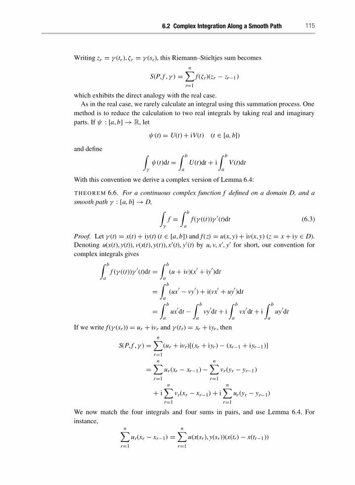
6.2 Complex Integration Along a Smooth Path 115
Writing zr = γ (tr), ζr = γ (sr), this Riemann–Stieltjes sum becomes
S(P, f ,γ ) =
n³
r=1
f (ζr)(zr − zr−1)
which exhibits the direct analogy with the real case.As in the real case, we rarely calculate an integral using this summation process. One
method is to reduce the calculation to two real integrals by taking real and imaginary
parts. If ψ : [a,b]→ R, let
ψ (t) = U(t)+ iV(t) (t ∈ [a, b])
and define ²
γ
ψ(t)dt =
² b
a
U(t)dt + i
² b
a
V (t)dt
With this convention we derive a complex version of Lemma 6.4:
THEOREM 6.6. For a continuous complex function f defined on a domain D, and asmooth path γ : [a, b] →D,
²
γ
f =
² b
a
f (γ ((t))γ ±(t)dt (6.3)
Proof. Let γ (t) = x(t)+ iy(t) (t ∈ [a,b]) and f (z) = u(x, y)+ iv(x, y) (z = x+ iy ∈ D).
Denoting u(x(t), y(t)), v(x(t), y(t)), x±(t), y±(t) by u, v, x±, y± for short, our convention forcomplex integrals gives
² b
a
f (γ ((t))γ±(t)dt =
² b
a
(u+ iv)(x±+ iy
±)dt
=
² b
a
(ux±− vy
±)+ i(vx
±+ uy
±)dt
=
² b
a
ux±dt −
² b
a
vy±dt + i
² b
a
vx±dt + i
² b
a
uy±dt
If we write f (γ (sr)) = ur + ivr and γ (tr) = xr + iyr , then
S(P, f ,γ ) =
n³
r=1
(ur + ivr)[(xr + iyr)− (xr−1 + iyr−1)]
=
n³
r=1
ur(xr − xr−1)−
n³
r=1
vr(yr − yr−1)
+ i
n³
r=1
vr(xr − xr−1) + i
n³
r=1
ur(yr − yr−1)
We now match the four integrals and four sums in pairs, and use Lemma 6.4. Forinstance,
n³
r=1
ur(xr − xr−1) =
n³
r=1
u(x(sr), y(sr))(x(tr) − x(tr−1))

116 Integration
where both φ(t) = u(x(t), y(t)) and x±(t) are continuous on [a,b]. So given ε > 0, we canfind a partition P1(ε) such that for any partition P that is finer than P1(ε) we have
´´´
n³
r=1
ur(xr − xr−1) −
² b
a
ux±dt
´´´ <
ε
4
Similarly we find partitions P2(ε),P3(ε), P4(ε) such that all finer partitions P give sim-
ilar inequalities between corresponding pairs of integrals and sums. Taking Pε to havedivision points all those of P1(ε), P2(ε),P3(ε),P4(ε), then whenever P is finer than Pε
all four inequalities hold. Therefore´´´S(P, f ,γ )−
² b
a
f (γ ((t))γ ±(t)dt
´´´ <
ε
4+ε
4+ε
4+ε
4= ε
Hence²
γ
f =
² b
a
f (γ ((t))γ ±(t)dt
Example 6.7. f (z) = z2,γ (t) = t2 + it (t ∈ [0, 1]). See Figure 6.2.²
γ
f =
² 1
0f (γ (t))γ
±(t)dt
=
² 1
0
(t2 + it)2(2t + i)dt
=
² 1
0
(t4 + 2it3 − t2)(2t + i)dt
=
² 1
0
(2t5 − 4t3)dt + i
² 1
0
(5t4 − t2)dt
= [ 13 t6− t4]10 + i[t5 − 1
3 t3]10
= − 23+
23i
Figure 6.2 Path for Example 6.7.

6.3 The Length of a Path 117
6.3 The Length of a Path
The length of a path is defined in terms of approximating polygons, as follows.
DEFIN IT ION 6.8. Given an arbitrary path γ : [a,b]→ C, take a partition P of [a,b]given by a = t0 < t1 < · · · < tn = b, and calculate the length
L(γP) =
n³
r=1
|γ (tr) − γ (tr−1)|
of the approximating polygonal curve γP with vertices γ (t0),γ (t1), . . . ,γ (tn), Fig-ure 6.3.
Figure 6.3 Length of a path as the supremum of the lengths of approximating polygons.
The length L(γ ) of γ is the supremum (least upper bound) of the lengths L(γP) overall such approximating polygons.
The length of an arbitrary path need not be finite:
Example 6.9. Suppose γ (t) (t ∈ [0, 1]) is defined as follows. Let mn be the midpoint of[1/(n+ 1), 1/n], so mn = (2n+ 1)/(2n(n+ 1)). Introduce a function λ where the graphof y = λ(t) consists of two straight line segments from ( 1
n+1 , 0) to (mn,1n ) and then to
( 1n , 0). Define
γ (t) =
µt + iλ(t) (0 < t ≤ 1)
0 (t = 0)
The image of γ is drawn in Figure 6.4.
Figure 6.4 A path with infinite length.

118 Integration
The length of this path from t =1
n+1to t =
1nexceeds 2
n. Let P be the partition
0 < 1n+1
< mn <1n< · · · < 1
2< m1 < 1. Then the length of the polygonal path
exceeds
2
n+
2
n− 1+ · · · +
2
1= 2
¶1+
1
2+
1
3+ · · · +
1
n
·
The latter is twice the harmonic series, so it increases without limit as n increases. There-fore L(γ ) is infinite.
In this example, the path is not smooth. The next example shows that even if the pathis ‘nearly smooth’, its length can still be infinite.
Example 6.10. Consider the path
γ (t) =
µt+ it sin(π/t) (0 < t ≤ 1)
0 (t = 0)
as in Figure 6.5.
Figure 6.5 A nearly smooth path with infinite length.
A calculation shows that although
γ ±(t) = 1+ i(sin(π/t) + t cos(π/t))(−π/t2)
is continuous for 0 < t ≤ 1, the limit of
γ (t)− γ (0)
t= 1+ i sin(π/t)
as t tends down to 0 does not exist. Hence γ ± is not continuous on the closed interval[0, 1], so is not smooth on [0, 1] (though it is smooth on any subinterval [k, 1] with0 < k ≤ 1).
We claim this path has infinite length. Let Pn be the partition
0 < 1/n< 1/(n− 12) < 1/(n− 1) < · · · < 1/2 < 1/(2− 1
2) < 1

6.3 The Length of a Path 119
Since
γ
¶1
n
·=
1
n+ i
sinnπ
n= 1/n
and
γ
¸1
n− 12
¹=
1
n− 12
+ isin(n−
12 )π
n− 12
=1
n− 12
+ i(−1)n−1
n− 12
the distance from γ (1/n) to γ (1/(n − 12)) exceeds 1/(n− 1
2), which exceeds 1/n. We
need only compute the lengths of alternate segments of the polygonal approximation γn
to γ given by Pn to find that
L(γn) >1
n+
1
n− 1+ · · · + 1
which again increases without limit.
6.3.1 Integral Formula for the Length of Smooth Paths and Contours
When a path is smooth, its length is finite, and can be calculated by an integral:
PROPOSIT ION 6.11. The length of a smooth path γ : [a, b] → C is
L(γ ) =
² b
a
|γ ±(t)|dt (6.4)
and this is finite.
We prove this result below, but first we note that the integrand |γ ±(t)| is continuous on[a,b], so the real integral
L=
² b
a
|γ ±(t)|dt
certainly exists, and is finite. We must show that L is the supremum of the lengths L(γP)of approximating polygons γP.Now L can be closely approximated by sums
S(P,φ) =
n³
r=1
|γ ±(sr)|(tr− tr−1)
where P is the partition a = t0 < t1 < · · · < tn = b, tr−1 < sr < tr , and φ(t) = |γ ±(t)|.

120 Integration
The proof of Proposition 6.11 is greatly facilitated by:
LEMMA 6.12. With the preceding notation, given any ε > 0, there exists a partitionQε such that for any partition P finer than Qε, the length L(γP) of the approximatingpolygon corresponding to P satisfies
|S(P, φ) − L(γP)| < ε
Proof. By definition,
S(P,φ) =
n³
r=1
|γ ±(sr)|(tr − tr−1)
L(γP) =
n³
r=1
|γ (tr) − γ (tr−1)|
Writing γ (t) = x(t)+ iy(t), the Mean Value Theorem in real analysis gives
x(tr) − x(tr−1) = x±(σr)(tr − tr−1) for some σr ∈ (tr−1 , tr)
y(tr)− y(tr−1) = y±(τr)(tr − tr−1) for some τr ∈ (tr−1 , tr)
so
γ (tr) − γ (tr−1) = (x±(σr) + iy±(τr))(tr − tr−1)
Now x±, y± are continuous on [a, b], and from real analysis they are uniformly continuoussince [a, b] is a closed interval. This means that for any ε > 0 there exists δ > 0 suchthat
s, t ∈ [a,b] and |s − t| < δ implies
|x±(s) − x
±(t)| < ε/2(b− a) and |y
±(s) − y
±(t)| < ε/2(b− a)
(where the same δ works for all s, t).If we choose Qε to be any partition such that each subinterval [tr−1 , tr] has length less
than δ , then any partition P finer than Qε has the same property. Because sr ,σr , τr ∈[tr−1 , tr], they are all within distance δ of each other, so
| |γ ±(sr)|(tr − tr−1) − |γ (tr)− γ (tr−1)| |= | |γ ±(sr)| − |x±(σr)+ iy
±(τr)| | (tr − tr−1)
≤ |(x±(sr) + iy±(sr))− (x±(σr)+ iy±(τr))| (tr − tr−1)
≤ (|x±(sr) − x±(σr)| + |y±(sr) − y±(τr)|)(tr − tr−1)
< (ε
2(b− a+
ε
2(b− a)(tr − tr−1)
= ε(tr − tr−1)/(b− a)
where in the third line we use property (1.12) of the modulus.
Thus
|S(P,φ)− L(γP)| ≤n³
r=1
| |γ ±(sr)|(tr − tr−1)− |γ (tr) − γ (tr−1)| |
<
n³
r=1
ε
b− a(tr − tr−1)

6.3 The Length of a Path 121
=ε
b− a
n³
r=1
(tr − tr−1)
= ε
as required.
We are now prepared for the following:
Proof of Proposition 6.11. Let L(γ ) be as in (6.4). By the definition of the Riemannintegral, there exists a partition P such that for any partition P finer than Pε,
|S(P,φ)− L| < ε (6.5)
Adding more division points to Pε as necessary to obtain a finer partition Qε with eachsubinterval of length less than δ, then for P finer thanQε , Lemma 6.12 gives
|S(P, φ) − L(γP)| < ε (6.6)
Combining this with (6.5) gives
L− 2ε < L(γP) < L+ 2ε (6.7)
Thus for any positive k we can find an approximating polygon γP with
L− k < L(γP) (6.8)
Given any partition Q of [a,b] with approximating polygon κ , the addition of furthervertices to κ can only increase its length, by the triangle inequality. Thus if P is finerthan Q then L(κ) ≤ L(γP). We choose P finer than Qε so that (6.7) holds; then
L(κ) ≤ L(γP) < L+ 2ε
But ε is any positive number, so for any approximating polygon κ ,
L(κ) ≤ L (6.9)
The inequalities (6.8) and (6.9) exhibit L as the supremum of the lengths of allapproximating polygons, completing the proof.
Example 6.13. The standard straight line path γ = [z1, z2]
γ (t) = z1(1− t) + z2t (t ∈ [0, 1])
has length
L(γ ) =
² 1
0
|γ ±(t)|dt =
² 1
0
|z2 − z1|dt = |z2 − z1|
as expected.
Example 6.14. The circle S(t) = z0 + reit (t ∈ [0, 2π]), centre z0 and radius r > 0, has
length
L(S) =
² 2π
0
|ireit| =² 2π
0
rdt = 2π r

122 Integration
6.4 If You Took the Short Cut . . .
Some readers will have read the previous three sections, and some will not. For the latter,we now give some basic definitions that are motivated by the previous three sections:
DEFIN IT ION 6.15. A path γ : [a, b] → C is smooth if γ ± exists and is continuous onthe closed interval [a,b].If D is a domain, the integral of a continuous function f : D→ C along the path γ is
²
γ
f =
² b
a
f (γ (t))γ ±(t)dt (6.10)
The length of γ is
L(γ ) =
² b
a
|γ±(t)|dt (6.11)
A comment on (6.10) and (6.11) is in order to explain what they mean. The integrandsf (γ (t))γ ±(t) and |γ ±(t)| are both continuous. The latter is real; the former may be writtenin real and imaginary parts as f (γ (t))γ ±(t) = U(t) + iV (t) and the integral
±γf can then
be calculated using two real integrals:²
γ
f =
² b
a
U(t)dt + i
² b
a
V (t)dt
Since all integrands involved are continuous, the real integrals all exist.At this stage, readers who made either choice are now equipped to proceed to the rest
of the book. If you took the short cut, take a quick look at Examples 6.13 and 6.14 toconvince yourself that the formula defining length makes sense for lines and circles.
6.5 Further Properties of Lengths
Recall from Definition 2.27 that paths can be added together if their start and end pointsmatch up correctly. Using approximating polygons, it is easy to prove that the lengthfunction L is additive:
PROPOSIT ION 6.16. If γ = γ1 + · · · + γn and L(γr) exists for 1≤ r ≤ n, then
L(γ ) = L(γ1)+ · · · + L(γn)
It is important to understand that the length of a path need not be the same as thelength of its image curve. In particular, this happens whenever the path ‘doubles backon itself’, as in the following example.
Example 6.17. Let σ : [−2, 2] → C be any smooth path. Let ρ : [−2, 2] → [−2, 2]be given by ρ(t) = t3 − 3t, which is a smooth map, and let γ = σ ◦ ρ. Then it canbe shown, using (6.4), that L(γ ) = 3L(σ ). The geometric significance of this result isstraightforward: as t increases from −2 to 2, the cubic t3 − 3t increases from −2 to 2,

6.5 Further Properties of Lengths 123
then decreases from 2 to−2, and finally increases from−2 to 2 again. So the path tracesthe curve three times.
Next, we consider how a change of parameter affects the length of a smooth path.
DEFIN IT ION 6.18. Smooth paths γ : [a,b]→ C, λ : [c,d] → C with the same image
curve C are smoothly equivalent parametrisations of C if there is a smooth functionρ : [a,b] → [c, d] with non-zero derivative ρ±(t) ²= 0 for t ∈ [a, b], where ρ(a) = c,
ρ(b) = d, and γ = λ ◦ ρ.
This relationship is an equivalence relation, because ρ−1 exists, is smooth, andalso has non-zero derivative, by the inverse function theorem. A smoothly equivalentparametrisation can be imagined as tracing the same curve in the same direction but atdifferent speeds.
PROPOSIT ION 6.19. If two smooth paths γ : [a, b] → C, λ : [c, d] → C are
smoothly equivalent parametrisations of the same curve C, then they have the samelength: L(γ ) = L(λ).
Proof. We have γ = λ ◦ρ where ρ : [a,b]→ [c,d] is a strictly increasing real functionwith continuous derivative ρ± on [a,b]. Therefore ρ±(t) ≥ 0, so ρ±(t) = |ρ±(t)|. Lets = ρ(t). Then as t increases from a to b, s increases from c to d and we can substituteds = ρ±(t)dt in the integral. The length of the path γ is therefore
L(γ ) =
² b
a
|γ ±(t)|dt
=
² b
a
|(λ ◦ ρ )±(t)|dt
=
² b
a
|(λ±(ρ(t))||ρ±(t)|dt
=
² b
a
|(λ±(ρ(t))|ρ±(t)dt
=
² b
a
|λ±(s)|ds = L(λ)
6.5.1 Lengths of More General Paths
You may be wondering why we require γ to be smooth in the definition of length inDefinition 6.15? Proposition 6.16 applies to contours made from several smooth pieces,which need not fit together smoothly where they join, so paths that are not smooth
can have meaningful lengths. Obviously, Definition 6.15 cannot be used for continuouspaths, because it involves the derivative of γ . But the definition ‘supremum of lengthsof all approximating polygons’, which occurs in the alternative treatment of Section 6.3,makes sense for any path, without assuming smoothness. However, this definition has itsown awkward features. Sometimes it goes wrong in the mild sense that the entire pathhas infinite length, as in Examples 6.9 and 6.10. However, it gets much worse. Using the

124 Integration
‘approximating polygon’ definition for length, there are continuous paths γ : [a, b]→ C
with the disturbing property that the length of any segment of the path, between pointsc < d in [a, b], is infinite.In fact, we have already met just such a path: the graph of the blancmange function,
Figure 4.3. Using dyadic rationals, it is straightforward to construct a sequence of par-titions of [c,d] such that the corresponding polygons have lengths tending to infinity.In fact, it is enough to do this for the graph of the blancmange function on the inter-val [0, 1], because we have already pointed out that this graph contains arbitrarily smallcopies of the graph of the blancmange function, and a small number times infinity isstill infinity. These copies are usually distorted by an affine transformation, but such adistortion keeps the length infinite. Similar remarks apply to space-filling curves, and tostandard fractals such as the snowflake curve, Mandelbrot [13], and Falconer [4].In other words, a path that is continuous but not smooth may not have a meaningful
length. This is probably counterintuitive, because we have been trained from an earlyage to assume that every linear object does have a length. The ancient Greeks worriedabout the length of the circumference of a circle without ever defining what they wereworrying about. It seemed obvious to them that any arc of a circle must have a length;their main aim was to find out what that length is. To do so, they tacitly assumed severalplausible properties, such as finding the length by using polygons to approximate the cir-cumference. Eventually mathematicians tightened up the logic, leading to Definition 6.8above, and understood what can go wrong.To complete the story, smoothness is not actually necessary for a path or curve to have
a well-defined length. There is a more general notion of a rectifiable curve, for which the‘approximating polygon’ definition is entirely satisfactory. However, the smooth case isall we need in this book.
6.6 Regular Paths and Curves
Just as we distinguish between a path γ and its image curve, we must distinguishbetween the derivative γ ±(t) and a tangent line to the curve. The derivative can be inter-preted as the velocity vector at time t for a point γ (t) moving along the curve. If γ ±(t) ²= 0it defines a tangent direction, hence a tangent line to the curve. When γ ±(t) = 0 it doesnot defines a tangent direction, so the curve may not have a tangent line. Section 6.7shows some of the things that can then happen.First, some standard terminology:
DEFIN IT ION 6.20. Let γ : [a, b]→ C be a smooth path.If t0 ∈ [a,b] and γ ±(t0) ²= 0, then t0 is a regular point of γ .If t0 ∈ [a,b] and γ ±(t0) = 0, then t0 is a singular point of γ .
When the image curve has a well-defined tangent line, it looks smooth: see Proposi-tion 6.22 below.The above discussion leads naturally to a special type of path or curve that will be
useful as we proceed, to relate the abstract theory to geometric intuition:
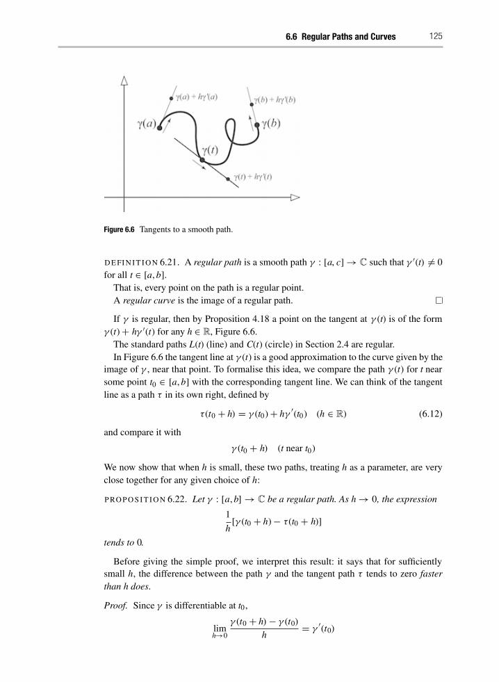
6.6 Regular Paths and Curves 125
Figure 6.6 Tangents to a smooth path.
DEFIN IT ION 6.21. A regular path is a smooth path γ : [a, c]→ C such that γ ±(t) ²= 0
for all t ∈ [a,b].
That is, every point on the path is a regular point.A regular curve is the image of a regular path.
If γ is regular, then by Proposition 4.18 a point on the tangent at γ (t) is of the formγ (t)+ hγ ±(t) for any h ∈ R, Figure 6.6.The standard paths L(t) (line) and C(t) (circle) in Section 2.4 are regular.In Figure 6.6 the tangent line at γ (t) is a good approximation to the curve given by the
image of γ , near that point. To formalise this idea, we compare the path γ (t) for t nearsome point t0 ∈ [a,b] with the corresponding tangent line. We can think of the tangentline as a path τ in its own right, defined by
τ(t0 + h) = γ (t0)+ hγ±(t0) (h ∈ R) (6.12)
and compare it withγ (t0 + h) (t near t0)
We now show that when h is small, these two paths, treating h as a parameter, are veryclose together for any given choice of h:
PROPOSIT ION 6.22. Let γ : [a,b] → C be a regular path. As h→ 0, the expression1
h[γ (t0 + h)− τ(t0 + h)]
tends to 0.
Before giving the simple proof, we interpret this result: it says that for sufficientlysmall h, the difference between the path γ and the tangent path τ tends to zero faster
than h does.
Proof. Since γ is differentiable at t0 ,
limh→0
γ (t0 + h) − γ (t0)
h= γ
±(t0)

126 Integration
Rewrite this as
limh→0
1
h[γ (t0 + h)− (γ (t0)+ hγ
±(t0))] = 0
By (6.12) this is the same as
limh→0
1
h[γ (t0+ h) − τ(t0 + h)] = 0
The proof does not use γ ±(t0) ²= 0; that is, the limit is still zero even when there is asingularity at t0. However, in that case τ (t0 + h) = γ (t0) for all h ∈ R. That is, τ does
not define a tangent line. So the result tells us nothing about the shape of the image of γnear t0 .
6.6.1 Parametrisation by Arc Length
Proposition 6.22 is a formal statement of the intuitive idea that a regular curve lookssmooth near any point. It has a continuously turning tangent and a well-defined finitelength. These properties are inherited by subpaths, leading to:
DEFIN IT ION 6.23. Let γ : [a,b] → C be a regular path, with image curve C. Lett0 , t1 ∈ [a,b] with t0 ≤ t1, and let γ (t0) = c,γ (t1) = d. Then the arc length LC(c, d)from c to d in C is the length of γ |[t0,t1]; that is,
LC(c,d) =
² t1
t0
|γ±(t)| dt
We now prove that a regular curve can be smoothly reparametrised so that the param-
eter t is arc length, or a constant multiple of arc length if that is more convenient. Letthe length of γ be L. Define λ : [a,b]→ [0,L] by
λ(s) = LC(a, s) =
² s
a
|γ ±(t)|dt
Then
λ±(t) = |γ ±(t)| ² = 0
so λ is a strictly increasing function on [a, b] with a continuous derivative λ± on [a,b],where λ(a) = 0, λ(b) = L. It is regular since λ±(t) ²= 0. It therefore has a strictlyincreasing inverse function ρ = λ−1 . Now ρ : [0,L] → [a,b] and has continuousderivative
ρ±(t) = 1/λ±(t) ²= 0
for a< t < b, so ρ is also regular.The path
τ = γ ◦ ρ : [0,L]→ C
is regular, and
τ(λ(t)) = γ ◦ ρ ◦ λ(t) = γ (t)

6.7 Regular and Singular Points 127
so τ is a reparametrisation of γ , with parameter λ(t) = LC(a, t). So τ reparametrises theimage curve C of γ by arc length. Moreover,
|τ±(t)| = |γ ±(t)||ρ±(t)| = |γ ±(t)|/|λ±(t)| = |γ ±(t)|/|γ ±(t)| = 1
So as t varies, τ (t) moves along the path with unit speed.Multiplying the parameter by a non-zero constant scales the speed 1 to any non-zero
constant speed, corresponding to a parameter that is a constant multiple of arc length.Any curve parametrised by arc length or such a multiple is regular.
6.7 Regular and Singular Points
Before tackling the intricacies of contour integration, we explain why the cases γ ±(t) ²= 0
and γ ±(t) = 0 differ significantly.Near a regular point, the image of γ is a smooth curve in the geometric sense that it
has a well-defined tangent direction (and this varies continuously). The curve may crossitself, but each separate segment near the crossing looks smooth.
Near a singular point, this may not be true. Sometimes there is a sensible, indeedvisible, tangent direction, but sometimes there is not. The geometry of γ (t) when t is
near a singular point t0 is highly sensitive to the precise behaviour of γ (t) when t is neart0 . We give a series of simple examples to illustrate some of the possibilities.
Figure 6.7 Examples of possible behaviour of a smooth path near a singular point. Left: Cusp.Right: Right-angled corner.
Example 6.24. Suppose that γ : [−1, 1] → C where γ (t) = t2 + it3. The derivative isγ (t) = 2t+3it2 , which is non-zero except at t = 0. The image is a semicubical parabolawith a cusp at the origin, Figure 6.7 (left). Everywhere else, the image is a smooth curve.The image has a natural tangent line at the cusp point, along the real axis, because this isthe limiting direction of tangents near the origin. However, the velocity vector reversesdirection as it passes through the origin.

128 Integration
To make sense of what is happening at a singular point we compare it with the realcase. In real analysis the graph of a function f : R → R consists of the points (x, f (x)) ∈R2 . If f is smooth, the graph has a well-defined tangent – even at a critical point wheref ±(x) = 0. However, if we imagine the point y = f (x) moving as x increases steadily, ybecomes stationary at any critical point. (Indeed, another term is stationary point.) Thetangent at a critical point is horizontal. This is the same as the direction in which a point(x, f (x)) on the graph is projected to obtain the image f (x). So the tangent projects to asingle point.The same kind of behaviour is happening at the cusp, but now γ is a hybrid function
with a graph γ : [−1, 1]→ C in coordinate form (t, t2 + it3) ∈ R×C. This is drawn inthe upper left part of Figure 6.8, represented in three-dimensional real space as (t, x, y) =(t, t2, t3), where t, x, y all lie between−1 and+1. Projection onto the vertical (x, y)-plane
project onto
vertical (x, y)-plane
x = t2
x = t2
x = t2
y=t3
y = t3
y = t3
0.5
0.5
tangent
–1
project
onto (t, x)-
3D (t, x, y)-space
–1
–1
–0.5–0.5
–0.5
0.5
t
t t
(x, y)-plane
(t, y)-plane(t, x)-plane
project sideways
onto (t, y)-planedown
plane
Figure 6.8 Example 6.24 represented in terms of the graph of the graph of the functionγ (t) = t2 + it3 in R× C pictured in R3 .

6.7 Regular and Singular Points 129
reveals the semicubical parabola (t2, t3); projection down onto the (t, x)-plane gives theparabola (t, x2); and sideways projection onto the (t, y)-plane gives the cubic curve (t, x3).The tangent at the origin is in the direction (1, 2t, 3t2) = (1, 0, 0), which points along thet-axis perpendicular to the complex plane and its projection onto the complex plane haslength zero.
Example 6.25. More surprisingly, the image can have a sharp corner, contrary to theintuition that it ought to at least look smooth.
Define φ : R→ R by
φ(t) =µ
0 (t ≤ 0)
t2 (t > 0)
This function is continuously differentiable because both 0 and t2 have the same
derivative, mainly 0, when t = 0.
Now define γ : [−1, 1]→ C by
γ (t) = φ(t)+ iφ(−t)
The image is then as shown in Figure 6.7 (right).The definition of φ can be modified to make γ infinitely differentiable, while retaining
the right-angled corner. Just change t2 to e−1/t as in (4.8).
Next we compare two different cases where the image of γ is a spiral.
Example 6.26. Suppose that
γ (t) =µ
0 (t = 0)
tei/t (t > 0)
Then γ : [0, 1] → C has a spiral image, Figure 6.9 (left). In this case, γ is notcontinuously differentiable. Indeed as t→ 0 from above, we have
γ±(t) = e
i/t + t.i
tei/t = (1+ i)e
i/t
This goes round and round the circle of radius |1 + i| =√2 at an ever-increasing rate,
so it does not tend to a limit as t→ 0. The one-sided derivative at t = 0 is not defined,let alone continuous.
Contrast this spiral with the following closely related one:
Example 6.27. Suppose that
γ (t) =µ
0 (t = 0)
t2ei/t (t > 0)
Then γ : [0, 1] → C has a spiral image, Figure 6.9 (right). The spiral is much tighterthan the previous example, and now γ is continuously differentiable. Indeed as t → 0

130 Integration
Figure 6.9 Left: A spiral path that is not smooth. Right: A smooth spiral path.
from above, we have
γ±(t) = (2+ i)te
i/t
which tends to 0 as t→ 0. The one-sided derivative at t = 0 is defined, and the derivativeis continuous there. As it happens, it is zero.
We now consider the lengths of the spiral paths in Examples 6.26 and 6.27, which canbe estimated by bounding the lengths of successive turns through 2π . In Example 6.26,turn n has length lying between two constant multiples of 1/n. So the total length liesbetween the same constant multiples of
∑n 1/n, the harmonic series, which is infinite.
In Example 6.27, turn n has length lying between two constant multiples of 1/n2. Since∑
n 1/n2 is finite, this spiral has finite length.
These results are consistent with the lack of smoothness of Example 6.26 (indeed,since its length is infinite Proposition 6.11 implies that it cannot be smooth), and thesmoothness of Example 6.27, which implies that its length must be finite.
6.8 Contour Integration
For readers who took the Riemann integral route, Section 6.2 defines the notion of asmooth path and deduces a formula for the integral along such a path. Those who optedfor the short cut should refer to Definition 6.15. For all readers, we now generalise thenotion of integration to allow paths made up of a finite number of smooth pieces:
DEFIN IT ION 6.28. Using the notation of Section 2.4, a contour is a path of the form
γ = γ1 + · · · + γn
where γ1, . . . ,γn are smooth paths such that the final point of γr coincides with the initialpoint of γr+1 for r = 1, . . . ,n− 1.

6.8 Contour Integration 131
Figure 6.10 The contour defined in Example 6.29.
Example 6.29. Let
γ1(t) = t (t ∈ [ε, R])
γ2(t) = R(cos t + i sin t) (t ∈ [0,π ])
γ3(t) = t (t ∈ [−R, ε])
γ4(t) = ε(− cos t + i sin t) (t ∈ [0,π ])
Then γ = γ1 + γ2 + γ3 + γ4 is the (closed) contour drawn in Figure 6.10.
6.8.1 Definition of Contour Integral
Integration along a contour is an easy extension of integration along a smooth path:
DEFIN IT ION 6.30. If D is a domain, f : D→ C is continuous, and γ = γ1 + · · · + γn
is a contour (so all γr are smooth), then the contour integral of f along γ is
²
γ
f =
²
γ1
f + · · · +²
γn
f
and
L(γ ) = L(γ1)+ · · · + L(γn)
It is obvious that if a smooth path σ is subdivided as
σ = σ1 + σ2
then ²
σ
f =
²
σ1
f +
²
σ2
f
so further subdivisions of the contours γ1 , . . . , γn in the above definitions will not affectthe values of the integrals. The contour integrals are therefore well-defined.The following standard properties hold, analogous to the real case:

132 Integration
PROPOSIT ION 6.31.²
γ1+γ2
f =
²
γ1
f +
²
γ2
f (6.13)
²
γ
( f1 + f2) =
²
γ
f1 +
²
γ
f2 (6.14)
²
γ
cf = c
²
γ
f (c ∈ C) (6.15)
²
−γ
f = −²
γ
f (6.16)
Proof. Equation (6.13) follows trivially from the definitions. The proofs of (6.14)and (6.15) depend on whether the reader has read Sections 6.1–6.3. If so, thenSection 6.2 implies that
S(P, f1 + f2, γ ) = S(P, f1, γ )+ S(P, f2 ,γ )
S(P, cf , γ ) = cS(P, f ,γ )
for any partition P, which imply (6.14) and (6.15).The reader who started from Section 6.8 can verify these formulas using known
properties of real integrals, as follows.First, it is sufficient to verify them for a single smooth path. To prove (6.14), observe
that
²
γ
( f1+ f2) =
² b
a
( f1(γ (t))+ f2(γ (t))γ±(t)dt
=
² b
a
f1(γ (t))γ±(t)dt +
² b
a
f2(γ (t))γ±(t)dt
=
²
γ1
f +
²
γ2
f
using the additivity property for real integrals on the real and imaginary parts.The proof of (6.15) is slightly longer (a minor penalty for skipping Sections 6.1–6.3),
because we must separate everything into real and imaginary parts. Let c = α + iβ ,
f (γ (t))γ ±(t) = U(t)+ iV (t). Then²
γ
cf =
² b
a
(α + iβ)(U(t) + iV (t))dt
=
² b
a
([αU(T )− βV (t)] + i[αV(t)+ βU(t)])dt
=
² b
a
[αU(T )− βV (t)]dt + i
² b
a
[αV(t)+ βU(t)])dt
= α
² b
a
U(T )dt − β
² b
a
V(t)dt + iα
² b
a
V(t)dt + iβ
² b
a
U(t)dt

6.9 The Fundamental Theorem of Contour Integration 133
= (α+ iβ)
² b
a
(U(t)+ iV(t))dt
= c
²
γ
f
using standard properties of real integrals.Finally, we prove (6.16). If γ : [a, b] → D is a contour, then the opposite path
−γ : [a, b] → D, defined by
−γ (t) = γ (a+ b− t) (t ∈ [a,b])
is also a contour. Now²
−γ
f =
² b
a
f (γ (a+ b− t))d
dtγ (a+ b− t)dt
= −² b
a
f (γ (a+ b− t))γ ±(a+ b− t)dt
Substituting s = a+ b− t this becomes
−
² a
b
f (γ (s))γ ±(s)(−ds)
= −² b
a
f (γ (s))γ ±(s)(ds)
= −²
γ
f
Therefore ²
−γ
f = −²
γ
f
6.9 The Fundamental Theorem of Contour Integration
Integrals of complex functions are only occasionally computed by breaking them downinto real and imaginary parts and calculating two real integrals as in the previous section.This technique is sometimes needed, but a far more efficient method is available for
±γ f
if we can find an antiderivative of f . This concept is so important that we give it a formal
definition:
DEFIN IT ION 6.32. Let D be a domain. An antiderivative for a function f : D → C is
a function F : D→ C such that F± = f .
An antiderivative, if it exists, is unique up to an added constant, for if F± = G± = f in
a domain, then (F −G)± = 0 so F − G is constant by Theorem 4.14. If we can find anantiderivative, then the integral can be computed immediately using:

134 Integration
THEOREM 6.33 (Fundamental Theorem of Contour Integration). If f : D → C is
continuous, F : D → C is an antiderivative of f , and γ is a contour in D from z0 to z1 ,then
²
γ
f = F(z1) − F(z0)
Proof. Let w(t) = u(t) + iv(t),W(t) = U(t) + iV(t) for t ∈ [a,b], where u, v,U,V are
real. Then W± = w if and only ifU ± = u,V ± = v, and then² b
a
w(t)dt =
² b
a
u(t)dt + i
² b
a
v(t)dt
= U(b)− U(a) + iV(b) − iV (a)
= W(b) −W(a)
Let w(t) = f (γ (t))γ ±(t). Since F± = f ,
w±(t) = F
±(γ (t))γ
±(t) = W
±(t)
where W(t) = F(γ (t)). Therefore²
γ
f =
² b
a
w(t)dt = W(b)−W(a)
= F(γ (b)) − F(γ (a)) = F(z1)− F(z0)
One remarkable feature of this result is that, in these circumstances, the integral doesnot depend on the path γ , only on its end points. In contrast, we show in Section 6.10that the integral may depend on the path when the conditions of Theorem 6.33 fail tohold.
Example 6.34. If f (z) = z2 and γ is any contour from z0 = 0 to z1 = 1 + i, thenF(z) = 1
3z3 is an antiderivative of f , and
²
γ
z2dz = 13(z31 − z30) =
13(1+ i)3 = 2
3+
23i
This example gives a visibly easier calculation than that performed at the end ofSection 6.2 for the particular contour γ (t) = t2 + it (t ∈ [0, 1]).However, any euphoria we feel over this phenomenon must be tempered with the
realisation that, unlike the real case where Theorem 6.2 (iii) tells us that a continuousfunction always has an antiderivative, in the complex case there are continuous func-tions without antiderivatives. Indeed, as we prove in Chapter 10, any function that isdifferentiable once in a domain is differentiable as many times as we wish. Now, anyantiderivative F must be differentiable once, so it is differentiable twice. Therefore itsderivative f = F± must be differentiable. So no non-differentiable function f has anantiderivative.

6.9 The Fundamental Theorem of Contour Integration 135
Example 6.35. We know that f (z) = |z|2 is differentiable only at the origin, so it isuseless to search for an antiderivative when integrating this f – for example along thepath γ (t) = t2 + it (t ∈ [0, 1]). In this case, we return to the basic formula
²
γ
|z|2dz =
² 1
0
(t4 + t2)(2t + i)dt
=
² 1
0
(2t5 + 2t3)dt + i
² 1
0
(t4 + t2)dt
= [ 13t6 + 1
2t4]10 + i[1
5t5 + 1
3t3]10
= 56+ 8
15i
Fortunately, many functions do have antiderivatives. For instance, by Corollary 4.5,any polynomial
p(z) = a0 + a1z+ · · · + anzn
has antiderivativep(z) = a0z+
12a1z+ · · · + 1
n+1anz
n+1
More generally, a power series has an antiderivative everywhere inside its disc ofconvergence:
THEOREM 6.36. If f (z) =∑∞
n=0 an(z − z0)n converges for |z− z0| < R, then
F(z) =
∞³
n=0
an
n+ 1(z− z0)
n+1
also converges for |z − z0| < R, and F ± = f .
Proof. It is sufficient to show that F(z) converges for |z − z0| < R, for then we may
differentiate term by term by Theorem 4.20 to obtain F± = f .
We know that the power series∑∞n=0 an(z−z0)
n converges absolutely for |z−z0| < R,
by Theorem 3.19. For each n, either an = 0 or|an(z− z0)
n/(n+ 1)|
|an(z − z0)n|
=|z − z0|
n+ 1
tends to zero as n→ ∞, so by the comparison test∑∞
n=0ann+1
(z−z0)n+1 converges.
If f (z) =∑∞n=0 an(z− z0)
n has disc of convergence D, then for any contour γ in D
from z1 to z2 ,²
γ
f =
∞³
n=0
an(z2 − z0)n+1
n+ 1−
∞³
n=0
an(z1 − z0)n+1
n+ 1
In particular, for any contour γ in D from z0 to z,
²
γ
f =
∞³
n=0
an(z− z0)n+1
n+ 1

136 Integration
6.10 An Integral that Depends on the Path
The Fundamental Theorem tells us that if a differentiable function f has an antiderivativethroughout its domain D, then the integral
±γ f is independent of the choice of path. This
applies to zn for any integer n ²= −1, with antiderivative zn+1/(n + 1) in the domain
C\{0}. It applies to 1/z2 , 1/z3, . . . but fails for 1/z, as we now show using formula (6.10).
Example 6.37. Consider the problem of integrating 1/z between −1 and 1. The pathalong the real axis passes through the origin, where 1/z is not defined, so we avoid thisby choosing a semicircular path.If the semicircle lies above the real axis (where im z ≥ 0) we can choose
γ1(t) = e−it (t ∈ [π , 2π ])
noting that e−iπ = −1, e−i2π = 1 and the −t makes the path run clockwise. Now²
γ1
1
zdz =
² 2π
π
1
γ1(t)γ ±1(t) dt
=
² 2π
π
1
e−it(−ie−it) dt
=
² 2π
π
−i dt
= [−it]2ππ
= −i(2π − π )
= −iπ
All very well, but we could equally sensibly choose the semicircle that lies below thereal axis (where im z ≤ 0). Now
γ2(t) = eit (t ∈ [π , 2π])
noting that eiπ = −1, ei2π = 1 and the +t makes the path run anticlockwise. A verysimilar calculation yields
²
γ2
1
zdz =
² 2π
π
1
γ2(t)γ±2(t) dt
=
² 2π
π
1
eit(ie
it) dt
=
² 2π
π
i dt
= [it]2ππ
= i(2π − π)
= iπ
which is slightly different.

6.11 The Gamma Function 137
At first it might appear that we made a mistake – it’s easy to get a sign wrong – butthe second integral is clearly the complex conjugate of the first, because everything isreflected in the real axis. Since neither is real, they cannot be equal.This example does not contradict Theorem 6.33 because 1/z does not have an
antiderivative in C\{0}. The obvious candidate is the logarithm, but by Section 5.7exp is periodic over C hence not one-one. Therefore any inverse ‘function’ to expmust be multivalued, as explained in detail in Section 7.3. So the logarithm is not anantiderivative over the whole of the domain.
In Chapter 8 we show that we get a different answer here because the point z = 0,
where 1/z is undefined, lies inside the region bounded by γ1 and γ2 . This behaviour isclosely connected to the multivalued nature of the complex logarithm. It has surprisinglyprofound implications, explored in Chapters 8–12.At any rate, this example should counteract any feeling that complex integrals are
always independent of the path, Theorem 6.33 notwithstanding.
6.11 The Gamma Function
So far the special complex functions that we have encountered are all extensions to C of
familiar real functions: polynomials, powers, trigonometric functions, the exponentialand the logarithm. In this section we briefly discuss a less familiar function, the gammafunction ±(z). This also began as a real function and was later extended to the complex
case. It has important applications, but we restrict attention to defining the function andestablishing a few basic properties. It will play a key role in Chapter 17 when we sketchconnections between complex analysis and number theory, culminating in the Riemann
Hypothesis.
The definition of the gamma function goes back to Euler, who initially defined it asthe infinite product
±(z) =1
z
∞º
n=1
Ȧ1+
1
n
·z ¼1+
z
n
½−1¾
This infinite product converges for all z ∈ C\{0,−1,−2 , . . .}. It defines a differentiablefunction on that domain, but we lack the techniques needed to prove this. Instead, weuse another formula due to Euler, who showed that when re z > 0 this is equal to theintegral
±(z) =
² ∞
0
tz−1e−tdt (6.17)
We take this as our definition, in order to illustrate complex integration. Here we define² ∞
0f = lim
a→∞
²
[0,a]f
so the interval [0,∞] is interpreted as the non-negative real axis. It is straightforwardto verify that (6.17) converges, because the factor e−t tends to zero rapidly. With thisdefinition, the formula (6.17) defines ±(z) only for z in the positive half-plane

138 Integration
C+ = {z ∈ C : rez > 0}
We establish some basic properties of ±(z) using methods from complex integration.First, we prove that the usual method of integration by parts generalises from real
analysis to the complex case:
THEOREM 6.38 (Integration by Parts). Let f ,g : D → C be differentiable functions onthe domain D. Then for any path γ : [a, b] → D we have:
²
γ
fg±= [fg]
ba−
²
γ
f±g (6.18)
Proof. By Proposition 4.4 (iii) we have
(fg)± = f ±g+ fg±
so
fg± = (fg)± − f ±g
Now integrate both sides over γ and use the Fundamental Theorem of ContourIntegration, Theorem 6.33.
Now we prove the basic functional equation for the gamma function:
THEOREM 6.39. If z ∈ C+ then
±(z + 1) = z±(z) ±(1) = 1 (6.19)
Proof. By (6.17), noting that z+ 1 ∈ C+, we have
±(z+ 1) =
²∞
0
tze−tdt
Now use integration by parts to rewrite this as
±(z+ 1) = [−tze−t]∞0 +
²∞
0
ztz−1e−tdt
= limx→∞
(−xze−x− (0e
0) + z
² ∞
0tz−1
e−tdt
= 0+ z
²∞
0
tz−1e−tdt
= z±(z)
To calculate ±(1), observe that
±(1) =
² ∞
0t1−1
e−tdt
= [−e−t]∞0
= 0− (−1)
= 1
By induction, this formula leads immediately to a curious result:

6.11 The Gamma Function 139
COROLLARY 6.40. If n ∈ N then
±(n) = (n− 1)!
In effect, the gamma function is a sensible way to define factorials for complex
numbers, in such a manner that the basic formula (n + 1)! = (n + 1)n! continues tohold.
6.11.1 Known Properties of the Gamma Function
We record (but do not prove) several other properties of the gamma function. One isEuler’s reflection formula
±(1− z)±(z) =π
sin πz
which is a consequence of his infinite product definition and a standard infinite productfor the sine. Setting z = 1
2 we obtain
(±( 12))2 = π
sin π/2= π
Therefore
±( 12 ) =√π
The duplication formula states that
±(z)±(z+ 12 ) = 21−2z
√π±(2z)
The derivative of the gamma function is obtained from the integral formula (6.17) by atechnique called ‘differentiating under the integral sign’, and leads to
± ±(z) =² ∞
0
tz−1e−t log t dt
(see Chapter 7 for the complex logarithm). This also proves that ± is a differentiablefunction in C+.Let γ be Euler’s constant, defined by
γ = limn→∞
¶1+ 1
2+ 1
3+ · · · + 1
n− log n
·∼ 0.577 216
Then
±±(1) = −γ
Weierstrass found another infinite product that works for all z ∈ C \ {0,−1 ,−2, . . .}:
1
±(z)= ze
γz
∞º
n=1
¿¼1+
z
n
½e−z/n
À
It is also possible to successively extend Euler’s formula to re z > −1, re z > −2, andso on, using (6.19) in the form
±(z− 1)=±(z)
z − 1

140 Integration
–5
–5
0
0
0
1
2
3
5
–5
–5
–5
–5
0
0
0
0
5
0.5
0.5
0.00.0
–0.5 –0.5
5
5
55
Figure 6.11 Graphs of (from left to right) the absolute value, real part, and imaginary part of thegamma function. Here x runs horizontally, y runs into the page, and the value of the functionconcerned runs vertically.
provided z − 1 ²= 0. This defines ± on the whole of the complex plane, except forthe points {0,−1,−2 , . . .}, and shows that the extended function is differentiable onits domain. It also explains why negative integers and zero must be excluded from thedomain, because ± would become infinite there; that is, have a pole. This procedure isan example of analytic continuation, which will be introduced in Chapter 14.Graphs of |±(z)|, re±(z), and im±(z) are shown in Figure 6.11, for this extended
domain.
The gamma function, and its poles, turned out to be an important ingredient in a rad-ical new development in complex analysis: an unexpected link with number theory. Inthe hands of Riemann and his contemporaries, this led to major advances in number the-ory, and a conjecture that remains one of the biggest unsolved problems in mathematics,the Riemann Hypothesis (see Chapter 17).
6.12 The Estimation Lemma
We now return to more general questions about complex integration, and prove a veryuseful technical result. Some results in mathematics are servants of the theory, of littleintrinsic interest in themselves, perhaps even a little dull, yet quietly figuring in impor-tant decisions all the time. ‘Always a lemma, never a theorem’. One such result is thelemma we are about to prove. It is a simple idea, giving an upper bound for the size ofan integral |
±γf | in terms of an upper bound on | f | and the length of γ , but it arises
time and again in the theory, applying subtle pressure at critical points in the proofs ofimportant theorems. Perhaps not a theorem of great stature, it is certainly worthy of aname. It is:
LEMMA 6.41 (Estimation Lemma). If f : D → C is continuous, γ is a contour oflength L, and | f (z)| ≤ M for all z on γ , then
´´²
γ
f
´´ ≤ ML
Proof. It is poetic justice that we have to give two different proofs, depending onwhether the reader has read Sections 6.1–6.3. Version A is the more natural, but it

6.12 The Estimation Lemma 141
requires knowledge of Sections 6.2–6.3. For readers who took the short cut, VersionB is provided.Version A. It is sufficient to prove the result for a smooth path γ : [a,b]→ D. Let P
be the partition a = t0 < t1 < · · · < tn = b, with tr−1 ≤ sr ≤ tr. Then
|S(P, f , γ )| =
´´´
n³
r=1
f (γ (sr))(γ (tr)− γ (tr−1))
´´´
≤
n³
r=1
| f (γ (sr))| |γ (tr)− γ (tr−1)|
≤ML(γP)
where γP is the polygonal approximation to γ with vertices γ (t0) , . . . ,γ (tn). ButL(γP) ≤ L(γ ), so
|S(P, f ,γ )| ≤ ML(γ ) (6.20)
for all partitions P.Given any ε > 0 we can find a partition Pε such that
´´S(Pε, f ,γ ) −
²
γ
f
´´ < ε
so ´´²
γ
f
´´ < |S(Pε, f ,γ )| + ε
and (6.20) gives ´´²
γ
f
´´ < ML(γ ) + ε
for all ε > 0. Hence ´´²
γ
f
´´ ≤ ML(γ )
as required.Version B. First we establish
´´´
² b
a
(u(t) + iv(t))dt
´´´ ≤
² b
a
|u(t) + iv(t)|dt (6.21)
for continuous real functions u, v. Let± b
au(t)dt = X,
± b
av(t)dt = Y. Then
² b
a
(u(t) + iv(t))dt = X + iY
and
X2 + Y2 = (X − iY )(X + iY ) =
² b
a
(X − iY)(u(t) + iv(t))dt
=
² b
a
(Xu(t)+ Yv(t))dt + i
² b
a
(Xv(t)− Yu(t))dt

142 Integration
But X2 + Y2 ∈ R, so² b
a
(Xv(t)− Yu(t))dt = 0
and
X2 + Y2 =
² b
a
(Xu(t)+ Yv(t))dt
where the integrand Xu(t)+ Yv(t) is the real part of (X − iY )(u(t) + iv(t)). So
Xu(t)+ Yv(t) ≤ |(X − iY)(u(t)+ iv(t))|
=ÁX2 + Y2|u(t)+ iv(t)|
From real analysis,² b
a
[Xu(t) + Yv(t)]dt ≤
² b
a
ÁX2 + Y2 |u(t)+ iv(t)|dt
which gives
X2 + Y2 ≤ÁX2 + Y2
² b
a
|u(t)+ iv(t)|dt
so thatÁX2 + Y2 ≤
² b
a
|u(t)+ iv(t)|dt (6.22)
But
ÁX2 + Y2 = |X + iY | =
´´´
² b
a
(u(t) + iv(t))dt
´´´
and with (6.22) this implies (6.21).Now
´´²
γ
f
´´ =
´´´
² b
a
f (γ (t))γ ±(t)dt
´´´
≤
² b
a
| f (γ (t))||γ ±(t)|dt by (6.21)
=
² b
a
|Mγ ±(t)|dt by real analysis
= ML
The Estimation Lemma will be used in a variety of ways. We now state twoapplications.
PROPOSIT ION 6.42. Let γ be a fixed contour and suppose that f varies.
(i) If the maximum value of | f | on γ tends to zero, then±γf → 0.
More generally, if f → f0 , then±γf →
±γf0 .
(ii) If the length of γ tends to zero, the image of γ tends to a point z0, and | f | remainsbounded, then
±γf → 0.
In particular this is the case if f is continuous at z0 .

6.13 Consequences of the Fundamental Theorem 143
Proof. To prove (i), observe that as the maximum value of | f | on γ tends to zero,|±γf | ≤ ML, which also tends to zero, so
±γf → 0.
The second statements follows by considering f − f0 .
To prove (ii), first observe that if f is continuous at z0, then | f | is bounded in a neigh-bourhood of z0. So we may assume | f | is bounded on γ . Again, |
±γf | ≤ ML, which
tends to zero.
6.13 Consequences of the Fundamental Theorem
If f is continuous and has an antiderivative F in a domain D, then we saw in Section 6.9that, for any contour γ in D from z0 to z1,
²
γ
f = F(z1) − F(z0)
This result has interesting consequences. To explore them we need:
DEFIN IT ION 6.43. A contour γ : [a, b] →C is a closed contour if γ (a) = γ (b).
In real analysis, an integral± a
a f is always zero. In the complex case, if f has anantiderivative in its domain D, then an integral
±γf round a closed contour inD is always
zero. (In the absence of an antiderivative, this need not be the case, as Example 6.37shows.) Moreover, if f has an antiderivative in D and z0 , z1 in D are different, it does notmatter which contour γ from z0 to z1 we use to integrate f : the result is always the same.
These properties characterise the existence of an antiderivative:
THEOREM 6.44. Let f be a continuous complex function defined on a domain D. Thenthe following conditions are equivalent:
(i) f has an antiderivative in D,(ii)
±γf = 0 for every closed contour γ in D,
(iii)±γf depends only on the end points of γ for any contour γ in D.
Proof. We have already established that (i) implies (ii) and (iii). To show that (ii) implies
(iii), suppose that γ1, γ2 are contours in D from z0 to z1, as in Figure 6.12.Then γ1 − γ2 is a closed contour, so by (ii)
±γ1−γ2
f = 0. But²
γ1−γ2
f =
²
γ1
f −
²
γ2
f
so ²
γ1
f =
²
γ2
f
which is (iii).Finally, to show that (iii) implies (i), we fix z0 ∈ D and for any z1 ∈ D we choose a
contour γ in D from z0 to z1 and define
F(z1) =
²
γ1
f

144 Integration
Figure 6.12 Two paths with the same end points determine a closed contour.
Because D is open, for some ε1 > 0, if |h| < ε1 then the line segment λ(t) = z1 + ht
(t ∈ [0, 1]) lies in D, and
F(z1 + h) =
²
γ1
f +
²
λ
f
Thus
F(z1 + h) − F(z1)
h=
1
h
²
λ
f
For any constant c and contour γ from z1 to z2,²
γ
cdz = c(z2 − z1)
so ²
λ
f (z1)
hdz = f (z1)
ThereforeF(z1 + h)− F(z1)
h− f (z1) =
²
λ
f (z)− f (z1)
hdz
Now we use the Estimation Lemma. Continuity of f implies that, given ε > 0, thereexists δ > 0 (which we may take to be less than ε1) such that
|z− z1| < δ implies | f (z) − f (z1)| < ε
so that, when 0 < |h| < δ, for any z on the line segment λ the integrand satisfies
|( f (z)− f (z1))/h| < ε/|h|
The length of λ is |h|, so whenever |h| < δ,´´²
λ
f (z) − f (z1)
hdz
´´ ≤
ε
|h||h| = ε
which implies ´´F(z1 + h)− F(z1)
h− f (z1)
´´ ≤ ε (|h| < δ)

6.13 Consequences of the Fundamental Theorem 145
But ε is arbitrary, so
limh→0
F(z1 + h) − F(z1)
h= f (z1)
and F±(z1) = f (z1) for z1 ∈ D, as required.
Example 6.45. The function f (z) = |z| is not differentiable, so±γ f may (and as we
show, does) depend on the choice of contour γ between points. For instance, considerγ , σ from 0 to i given by
γ (t) = it (t ∈ [0, 1])
and σ = σ1+ σ2 where
σ1(t) = t (t ∈ [0, 1])σ2(t) = eit (t ∈ [0,π/2])
as in Figure 6.13. Then²
γ
|z|dz =
² 1
0
|it| · idt =Âit2/2
Ã10= 1
2i
but²
σ
|z|dz =
² 1
0
|t| · 1 dt +² π/2
0
|eit | · ieit dt =Ât2/2
Ã10+ÂeitÃπ/20= 1
2+ i− 1= i − 1
2
Figure 6.13 Two paths γ and σ1 + σ2 that yield different values of the integral of |z|.
While complex functions that are merely continuous may be integrated using the basicformula, they offer little of interest. From now on, differentiable functions, and methods
for integrating them, occupy centre stage. The resulting theory of integration has nonatural real counterpart, because the real line lacks the flexible choice of path betweenpoints that occurs in the complex plane.With minor exceptions, this chapter completes the natural analogies between the real
and complex theories of differentiation and integration. From now on, new possibilitieswill unfold.

146 Integration
6.14 Exercises
1. Draw the contours γ = [0, i], σ = [0, 1]+ [1, i]. Evaluate²
γ
re zdz
²
σ
re zdz
2. Draw the contours γ = [−i, i] and σ where σ (t) = eit (t ∈ [−π/2,π/2]). Evaluate²
γ
|z|dz²
σ
|z|dz
3. Compute±γ z
4dz for γ (t) = (1+ i)t (t ∈ [0, 1]) using the formula
²
γ
f (z)dz =² 1
0f (γ (t))γ
±(t)dt
and multiplying out the right-hand side and integrating the real and imaginary parts.If γ = [0, 1]+ [1, 1+ i], what is
±γ z
4dz?
4. Let n be a positive integer. If γ (t) = z0+ reit (t ∈ [0, 2nπ ]) describe the contours γand −γ geometrically. Compute
²
γ
1
z− z0dz and
²
−γ
1
z− z0dz
5. For γ (t) = eit (t ∈ [0,π ]) evaluate±γ f for each of the following functions f :
(i) 1/z2
(ii) 1/z(iii) cos z(iv) sinh z(v) tan z(vi) (exp(z))3
6. Verify that the length function L satisfies
L(−γ ) = L(γ ) L(γ + σ ) = L(γ )+ L(σ )
where γ ,σ are contours.7. Let γ (t) = z0 + reit (t ∈ [0, θ]) be the arc centre z0 , radius r, subtending angle θ .
Using Proposition 6.11, verify that
θ = L(γ )/r
which is the usual definition of ‘angle θ in radian measure’.
8. Show that the length of the parabolic arc γ (t) = at2 + 2ait (t ∈ [0, 1]), where0 < a ∈ R, is
a(√
2+ log(1+
√2))
9. If γ is a closed contour in C, the signed area enclosed by γ is defined to be
S = 1
2i
²
γ
zdz

6.14 Exercises 147
Figure 6.14 What does the signed area represent for this contour?
By writing the integral explicitly in the form± b
a (u−iv)(u±+iv±), or otherwise, showthat S is real. Show that its value for circular and triangular contours is ³ the usualarea, and that both signs can occur. What is the geometric significance of the sign?What does the signed area represent for a contour such as Figure 6.14?
10. Show that the signed area in Exercise may also be given by
S = −²
γ
im z dz S =1
i
²
γ
re z dz
Write down the value of the integral±γ im z, where γ is the square γ = [0, 1] +
[1, 1+ i] + [1+ i, i] + [i, 0].
11. Let γ (t) = eit (t ∈ [0,π/2]). Use integration by parts, Theorem 6.38, to compute
(i)±γ z sin zdz
(ii)±γ z cos z dz
(iii)±γ ze
iz dz
(iv)±γ z
2 sin z dz
12. Let cr(t) = z0 + reit (t ∈ [0, 2π]) be the circle centre z0 , radius r > 0. If f is
continuous in the domain D and z0 ∈ D, use the Estimation Lemma to prove
(i) limr→0
²
Cr
f (z)dz = 0
(ii) limr→0
²
Cr
f (z)
z − z0dz = 2πif (z0)
13. For each of the following functions f : D → C, either state an antiderivative F :
D→ C or explain why an antiderivative does not exist.(i) f (z) = z2 , D = C
(ii) f (z) = 1/z2, D = C \ {0}(iii) f (z) = 1/z, D = C \ {0}(iv) f (z) = z sin z, D = C
(v) f (z) = |z|2, D = C(vi) f (z) = z, D = C

148 Integration
–4 –3–4½
–3½
–2½ –1½ –½ ½ 1½ 2½ 3½–2 –1 1 2 3 4 x
x!
10
–10
20
–20
Figure 6.15 Graph of x! for real x.
14. Use Euler’s reflection formula
±(z)±(1− z) =π
sin(π z)
to find ±( 12). Use the identity ±(z+ 1) = z±(z) to calculate ±(n+ 1
2) for all n ∈ N.
Gauss’s pi function has the value ²(z) = ±(z + 1) and is known to be analyticin D = C \ {n ∈ Z : n < 0}. By translating the identity ±(z + 1) = z±(z) to²(z) = z²(z − 1) show that ²(0) = 1 and ²(n) = n! for n ∈ N.
Figure 6.15 shows the graph of x! for real values of x. Calculate the numericalvalues of (n+ 1
2)! for n = 0, 1, 2, 3,−1,−2,−3,−4, and mark them on the graph.

7 Angles, Logarithms, and the WindingNumber
So far, we have defined complex analogues of most of the basic special functions of realanalysis – the exponential and trigonometric functions – and proved that many of theirfamiliar properties extend to the complex case. Some new features also arise, such asthe link between exponential and trigonometric functions and the periodicity of exp.There is one glaring exception to our catalogue of complex analogues: the loga-
rithm. In real analysis, we define this as the inverse function to exp : R → R+, so
log : R+ → R. However, because exp is periodic in C, it is not one-one (injec-tive). Therefore it does not have an inverse function in the strict set-theoretic sense.This feature caused many of the historical disagreements about logarithms of nega-tive and complex numbers, exacerbated by the general view that log z is automatically
meaningful when z ∈ C, and all of its properties ought to generalise to C.Resolving these issues involves being far more careful when defining complex log-
arithms. But the effort is worthwhile, because logarithms hold the key to many of thedeeper and more powerful features of complex analysis.The problem of finding inverses to functions that are not bijections arises in real
analysis as well. Inverse trigonometric functions such as sin−1 are notorious for causingsevere headaches, but the square root is the most obvious case. The square f (x) = x2 is
not injective as a function f : R → R. It is also not surjective: negative real numbers arenot squares of real numbers. The historical resolution was to define two square roots forevery positive real number, ±
√x. Each is a one-sided inverse: (±
√x)2 = x when x > 0.
But neither is an inverse on the domain of f , which is all of R: their images are thepositive reals and the negative reals, respectively, so they are not surjections onto R. Toobtain genuine inverse functions, we restrict the domain of f to the non-negative reals,when
√x is an inverse, or to the non-positive reals, when −
√x is an inverse. These two
domains meet only at the origin.It would be natural to try the same trick in the complex case. But now there is no very
natural way to restrict the domain and codomain to make the logarithm a bijection. Avariety of more or less artificial choices exist, such as the ‘cut plane’ Cπ where the neg-ative real axis is deleted, and these have their uses. To obtain a natural description of thecomplex logarithm, though, we use a more geometric approach. In classical terms, thecomplex logarithm is ‘multivalued’ – its value is not uniquely defined. The way in whichits multiplicity of values fit together is closely analogous to the way that the measure-
ment of an angle in radians gives not a single real number, but an infinite list differingonly by multiples of 2π. Indeed, these two instances of non-uniqueness are closely

150 Angles, Logarithms, and the Winding Number
related. In particular, the well-known complications when defining inverse trigonomet-
ric functions in real analysis also arise because these functions are 2π -periodic, hencenot injective. The same issue has to be resolved to make sense of the complex logarithm.
We discuss these ideas below, and apply them to a topological invariant known asthe winding number of a path relative to a point z0 ∈ C. In essence, this measures thetotal angle relative to z0 traversed by a point moving along the path continuously frombeginning to end. When divided by 2π , this angle tells us how many times the pathwinds round the point z0 . The winding number proves to be extremely useful in thedeeper parts of the subsequent theory.
7.1 Radian Measure of Angles
We first relate the power series definitions of sine (5.7) and cosine (5.8) to the usualgeometric ones, with the angle being measured in radians. This completes the proof thatthe power series represent the traditional trigonometric functions in the real case.Let 0 ²= z ∈ C and write z in polar coordinates as z = reiθ , (r > 0). Since eiθ =
cos θ + i sin θ , Table 5.1 in Section 5.5 implies that for fixed r, as θ increases from 0to π/2, the real part of z decreases monotonically from r to 0 while the imaginary partincreases monotonically from 0 to r. Since |z|2 = r2(cos2 θ + sin2 θ ) = r2 , it followsthat z traces out the first quadrant of a circle of radius r (in the anticlockwise direction)as θ increases from 0 to π/2, Figure 7.1 (left).Similarly, as θ increases from π/2 to π , the point z traces out the second quadrant
of a circle of radius r; from π to 3π/2, it traces out the third quadrant; from π to
3π/2, it traces out the fourth; and thereafter it continues to go round the circle in theanticlockwise direction, Figure 7.1 (middle).
We now compute the arc length from 1 to z along the circular path. For θ ≥ 0, letγ (t) = reit, (t ∈ [0, θ]). Then γ is a contour from 1 to z along the relevant arc. Thelength of γ is
Figure 7.1 Left: reiθ traces out the first quadrant of a circle of radius r as θ increases from 0 toπ/2. Middle: For θ ∈ R, reiθ repeatedly traces out the circle of radius r in the anticlockwisedirection. Right: Traditional geometric definitions of sinθ and cos θ agree with the power seriesdefinitions.

7.2 The Argument of a Complex Number 151
L(γ ) =
± θ
0
|γ ³(t)|dt =
± θ
0
|ireit|dt =
± θ
0
rdt = rθ
Thus θ = L(γ )/r, which is the standard definition of ‘angle measured in radians’.Figure 7.1 (right) then shows that the geometric definitions of sin θ and cos θ , in terms
of a right triangle with an angle θ radians, agrees with our analytic definition via powerseries.
The 2π -periodicity of sin and cos proved in Proposition 5.5 shows that this agreement
extends to angles greater than 2π , and to negative angles, which of course are measured
in the opposite sense round the circle: clockwise.
7.2 The Argument of a Complex Number
We now look in more detail at the expression of a complex number z in the form reiθ .
Here r = |z|, so it is unique. However, when r = 0 any value of θ leads to z = 0.
And when r > 0 there are infinitely many possible values of θ , differing only by integermultiples of 2π. Recall that the unique value in the range −π < θ ≤ π is called theprincipal value of the argument of z, and is denoted by
arg z
This defines a function
arg : C \ {0} :→ R
The function arg is not continuous on the negative real axis. This is a result of the needto choose θ uniquely: just above the axis θ is close to π , just below it is close to −π .We can sidestep this problem (inelegantly) by defining the cut plane
Cπ = C \ {x + iy : y = 0,x ≤ 0}
as in Figure 7.2.We claim that arg is continuous in the cut plane. This is plausible geometrically, but
we must provide a rigorous proof. There is one technical difficulty: the bad behaviour of
Figure 7.2 The cut plane Cπ .

152 Angles, Logarithms, and the Winding Number
inverse trigonometric functions (also caused by periodicity). We circumvent it by usingseveral overlapping domains, on each of which the behaviour is sufficiently good. Theproof that follows is an inelegant ‘bare hands’ reduction to properties of real functions:for a more elegant approach see Section 8.4.
PROPOSIT ION 7.1. The function arg is continuous in the cut plane Cπ .
Proof. Let
D1 = {x + iy ∈ C : y > 0}
D2 = {x + iy ∈ C : x > 0}
D3 = {x + iy ∈ C : y < 0}
Then
C = D1 ∪ D2 ∪D3
(draw a picture!) and in each of these domains we have an easy way to find the value ofarg z.
To do so, observe that ifz = x+ iy = eiθ
and we wish to solve for r, θ , then
r2 = x2 + y2 so r =
²x2 + y2
and
cos θ =x
³x2 + y2
sin θ =y
³x2 + y2
From properties of sin and cos it follows that if z ∈ D1 there is a unique solution for θwith 0 < θ < π . In this range cos is monotonic strictly decreasing and continuous, soits restriction to (0,π ) has a continuous inverse function
cos−1 : (−1, 1)→ (0,π )
For z ∈ D1 we have
arg z = cos−1re z
|z|
which, being a composition of continuous functions, is continuous.Similarly if x ∈ D2 then−π/2 < θ < π/2. In this range, sin increases monotonically
from−1 to 1, so it has a continuous inverse
sin−1
: (−1, 1)→´−π
2,π
2
µ
Now
arg z = sin−1im z
|z|
which is continuous on D2.

7.3 The Complex Logarithm 153
Figure 7.3 The cut plane Cα.
Finally, on D3 we can use
cos−1
: (−1, 1)→ (−π , 0)
which is a different choice of inverse cosine from that used in D1 because we areinverting the restriction of cos to a different interval. Again arg is continuous on D3.
Since D1 ,D2,D3 are open, arg is continuous in D1 ∪D2 ∪ D3 = Cπ .
It is sometimes convenient to proceed more generally. Let α ∈ R, and let Rα be theray
Rα = {reiα : r ≥ 0} ⊆ C
Let
Cα = C \ Rα
as in Figure 7.3. Chooseθ = arg
αz (z ∈ Cα)
by the rulez = reiθ , r > 0, α− 2π < θ < α
Then by a similar method it may be shown that arg is continuous in Cα .
7.3 The Complex Logarithm
The complex logarithm poses similar problems, because the complex exponentialfunction is not one-one.We wish to define log z, for 0 ²= z ∈ C, by
w = log z if z = ew
(We exclude z = 0 because ew is never zero, by Proposition 5.4.)

154 Angles, Logarithms, and the Winding Number
Let z = reiθ , w = u + iv. (The mixture of polar and Cartesian coordinates isdeliberate!) We assume r > 0, −π < θ ≤ π, so θ = arg z. Then z = ew becomes
reiθ = eu+iv (7.1)
Taking moduli,
r = eu (7.2)
Since r > 0 and r,u ∈ R this has the unique solution
u = log r
where log is the real natural logarithm. Then (7.1) and (7.2) imply that
eiθ = eiv
so thatv = θ + 2nπ (n ∈ Z)
Hence
log z = w = log r + i(θ + 2nπ )
or
log z = log |z| + i(arg z+ 2nπ ) (7.3)
The complex logarithm is thus ‘multivalued’ and therefore not a function in the strictset-theoretic sense. To obtain a genuine (single-valued) function we define the principalvalue of the logarithm to be
Log z = log |z| + i arg z (0 ²= z ∈ C)
(Note the capital ‘L’ for the principal value.) This function is not continuous on thenegative real axis. However, for z ∈ Cπ the real and imaginary parts of Log are clearlycontinuous, so Log is continuous in the cut plane.Now we can compute the derivative of the logarithm. We have
d
dzLog z0 = lim
z→z0
Log z− Log z0
z− z0
= limw→w0
w− w0
ew − ew0
setting z = ew , z0 = ew0 and using continuity of Log. Thus
1ddzLog z0
= limw→w0
ew − ew0
w − w0=
d
dzexpw0 = e
w0
andd
dzLog z0 =
1
ew0=
1
z0
and in generald
dzLog z =
1
z(z ∈ Cπ)

7.4 The Winding Number 155
In the same way, in the cut plane Cα we can define
logα z = Log |z| + i argα z
and this is continuous, with derivatived
dzlogα z =
1
z(z ∈ Cα)
Once the logarithm is defined, powers za for complex a can be defined, in a cut plane,by reducing them to exponentials. The principal value of za, when z ²= 0, is
za = exp(aLog z)
Exercises 9–14 of Section 7.9 explore this function. For a more global view of za see
Chapter 14.
7.4 The Winding Number
Suppose that γ : [a,b]→ C\ {0} is a closed path. The choice of codomain here ensuresthat the path does not pass through the origin. If we imagine t, the parameter, to be time,
increasing from a to b, and choose the argument θ(t) of γ (t) to vary continuously witht, then as γ (t) moves along the path, then intuitively the total change in argument is thenumber of times that γ winds round the origin (anticlockwise), multiplied by 2π. (If γis not closed this can also be defined, but it need not be an integer.)We wish, of course, to make this idea precise:
DEFIN IT ION 7.2. A continuous choice of argument along a path γ : [a, b] → C \ {0}(which for full generality we no longer require to be a closed path) is a continuousmap
θ : [a,b]→ R such that
eiθ(t) =γ (t)
|γ (t)|(7.4)
Condition (7.4) merely says that θ (t) is one of the possible values of the argument ofγ (t).
Before proving that a continuous choice of argument exists, in Theorem 7.4 below,we consider a simple example.
Example 7.3. Let γ (t) = reit (t ∈ [0,π ]), Figure 7.4.A continuous choice of argument is θ(t) = t, because obviously reit/|reit| = eit =
reiθ (t) . But this is not the only possible choice: θ (t) = t + 2π works equally well, orindeed θ(t) = t + 2nπ for any fixed n ∈ Z.What we cannot do is ‘change horses in midstream’, say by choosing
θ(t) =
¶t (t ∈ [0,π/2])
t + 2π (t ∈ (π/2,π ])
If we do that, condition (7.4) holds, but θ is not continuous.

156 Angles, Logarithms, and the Winding Number
Figure 7.4 A semicircular path.
The difficulty (though it does not take much getting used to) in handling continuouschoices of argument is that it does not in general suffice to insist on some simple recipefor choosing a value of the argument, such as keeping angles between 0 and 2π . Sucha choice becomes discontinuous if the path winds round once anticlockwise, taking theargument to 2π , and then continues in the anticlockwise direction. Then the argument
jumps discontinuously back to near 0 when we want it to continue increasing from 2π .It turns out that we can choose the argument at the starting point to be any of
the infinitely many possible values; but this choice then determines all of the restuniquely – and the arguments that arise need not stay within any predetermined range.It is intuitively obvious that this kind of choice can be made, and that it is unique oncewe decide where to start. Its proof is a little tricky: it uses the Paving Lemma.
THEOREM 7.4. (i) Let γ : [a,b]→ C \ {0} be a path not passing through the origin.Then there exists a continuous choice of argument for γ .
(ii) Any other continuous choice of argument differs from this by a constant integermultiple of 2π .
Proof. By the Paving Lemma 2.33 we can subdivide γ into finitely many subpathsγr (r = 1, . . . , n) such that each γr lies inside a disc Dr ⊆ C \ {0}, Figure 7.5. Ifthe centre of dr is at ρreiθr , then taking αr = θr + π , we find that Dr ⊆ Cα , so argα is
continuous in Dr .
This gives a continuous choice of argument across γr for each r, but of course thesechoices need not fit together continuously. However, any choice of argument can beobtained from any other by adding a suitable integer multiple of 2π. We can thereforeadjust the argαr inductively so that they do fit together continuously, as follows.As usual, let γr be defined on the parametric interval [tr−1, tr]. There is an integer n2
such that
argα1(t1) = argα2(t1) + 2n2π
Then there is an integer n3 such that
argα2(t2)+ 2n2π = argα3(t2)+ 2n3π

7.4 The Winding Number 157
Figure 7.5 Paving a path.
and so on inductively, choosing nr+1 so that
argαr (tr) + 2nrπ = argαr+1 (tr) + 2nr+1π
Then we define
θ(t) = argαr(tr)+ 2nr2π (t ∈ [tr−1 , tr])
with n1 conventionally defined to be 0. Then θ is continuous. This proves that acontinuous choice of argument exists.Next, suppose that θ∗ is another continuous choice of argument. Then we must have
θ∗(t) = θ(t)+ 2n(t)π
where n(t) is an integer, possibly depending on t. But
n(t) =θ∗(t) − θ(t)
2π
is continuous, yet takes integer values. It is therefore constant.
Note that a continuous choice of argument is defined on the parametric interval [a,b],not on the image of γ . This means that if the path returns to the same point, with γ (t1) =γ (t2) but t1 ²= t2, the arguments θ(t1) and θ(t2) may be different. Intuitively, it is clearthat this will happen if the path winds round the origin a non-zero number of times
between t1 and t2 .
Example 7.5. Let γ (t) = re4π it (t ∈ [0, 1]).A continuous choice of argument is given by θ (t) = 4π t + 2nπ, for any choice of
n ∈ Z. Although γ (t) = γ (t+ 12) for t ∈ [0, 1
2], the choices of argument θ(t) and θ(t+ 1
2)
differ by 2π , because the path has travelled once round the origin (anticlockwise)between t and t + 1
2 .

158 Angles, Logarithms, and the Winding Number
More significantly, γ (0) = γ (1), but the difference in arguments is 4π , because intotal the path has travelled twice round the origin (anticlockwise) between t = 0 andt = 1.
We can take advantage of this idea:
DEFIN IT ION 7.6. The winding number of a path γ : [a,b]→ C \ {0} round the originis
w(γ , 0) =θ(b)− θ (a)
2π
for a continuous choice of argument θ along γ .
By Theorem 7.4 (ii) the winding number is well defined; that is, any continuous choiceof argument gives the same value.For any closed path, the winding number is an integer, because θ (b) − θ(a) is an
integer multiple of 2π.The winding number takes the sense of the path into account: anticlockwise turns
count as positive, clockwise turns count as negative.
Example 7.7. Let γ (t) = re−it (t ∈ [0, 6π ]).A continuous choice of argument is θ(t) = −t. Then
w(γ , 0) = θ(6π) − θ(0)
2π= −3
and γ winds three times round the origin in the clockwise direction.
The winding number is additive:
THEOREM 7.8. Let γ1 and γ2 be two paths in C \ {0} such that the end point of γ1 isthe start of γ2 . Then
w(γ1 + γ2 , 0) = w(γ1, 0) + w(γ2, 0)
Proof. We may assume that γ1 ,γ2, and γ1 + γ2 have parametric intervals [a,b], [b, c],and [a, c] respectively. Let θ be a continuous choice of argument on γ1 + γ2 . Then
w(γ1 + γ2, 0) =θ(c) − θ(a)
2π
w(γ1, 0) =θ(b) − θ(a)
2π
w(γ2, 0) =θ(c) − θ(b)
2π
This is an extremely useful result, because it lets us compute the winding number ofa complicated path by breaking it up into nice pieces and adding their contributions. Itextends easily to show that
w(γ1 + · · · + γn , 0) = w(γ1, 0) + · · · +w(γn , 0)
and thatw(−γ , 0) = −w(γ , 0)

7.6 The Winding Number Round an Arbitrary Point 159
7.5 The Winding Number as an Integral
If the path is smooth, we can specify its winding number as an integral along the path.Additivity of the winding number extends this formula to contours. First, consider aclosed contour.
THEOREM 7.9. Let γ be a closed contour. Then
w(γ , 0) = 1
2π i
±
γ
1
zdz (7.5)
Proof. Subdivide the path into subpaths γ1 , . . . , γn as in Theorem 7.4, whose notationwe now use. Each γr lies in a cut plane Cαr . If γr is defined on the interval [tr−1 , tr] then
±
γr
1
zdz = logαr γ (tr)− logαr γ (tr−1)
= log |γ (tr)| − log |γ (tr−1)|
= i(argαr |γ (tr)| − argαr |γ (tr−1)|)
As in Theorem 7.4 we make sure that argαr γ (tr) = argαr+1 γ (tr), that is, the choicesof argument agree where the subpaths join together. Then, summing the integrals forr = 1, . . . ,n, the real parts cancel out because γ is a closed contour, and the imaginary
parts add up to 2πw(γ , 0), as required.
7.6 The Winding Number Round an Arbitrary Point
There is nothing very special about the origin as far as winding numbers are concerned.If γ : [a, b] → C is a path and z0 ∈ C does not lie on γ , we can define the windingnumber of γ around z0. The easiest way to do this is to translate the origin, setting
±(t) = γ (t)− z0 (t ∈ [a, b])
and calculatingw(γ , z0) = w(±, 0)
For a closed path γ , we get
w(γ , z0) =1
2π i
±
±
1
zdz
=1
2π i
± b
a
±³(t)
±(t)dt
=1
2π i
± b
a
γ ³(t)
γ (t)− z0dt
=1
2π i
±
γ
1
z− z0dz
This leads to:

160 Angles, Logarithms, and the Winding Number
DEFIN IT ION 7.10. If γ : [a,b] → C is a closed path and z0 ∈ C does not lie on γ ,then the winding number of γ around z0 is
w(γ , z0) =1
2π i
±
γ
1
z− z0dz (7.6)
The additivity of w(γ , 0) in Theorem 7.8 extends easily to w(γ , z0) for fixed butarbitrary z0 ∈ C, using the same trick of translating the origin.
7.7 Components of the Complement of a Path
We consider how the winding number w(γ , z0) of a given closed path γ can vary as z0varies.
By Proposition 2.41, the complement S of the image of γ is open, and also each con-nected component of S is open. The winding number w(γ , z0) is defined for all z0 ∈ S,
and it is an integer-valued function on S. It is geometrically plausible that this functionis constant on any connected component of S. We prove this analytically by showingthat w(γ , z0) is a continuous function of z0 ∈ S. The desired result then follows, sinceany integer-valued continuous function is constant on any connected set.The proof that w(γ , z0) is continuous in z0 is obtained by a direct estimate. Fix z0 ∈ S.
Since S is open there exists k > 0 such that |z1 − z0| < k implies z1 ∈ S. Therefore if zlies on the image of γ then |z− z0| ≥ k. Thus if |z1− z0| < k/2 we have |z− z1| > k/2.
Now
|w(γ , z0)− w(γ , z1)| =1
2π
····±
γ
¸1
z− z0−
1
z − z1
¹dz
····
=1
2π
····±
γ
z1 − z0
(z− z0)(z− z1)dz
····
≤|z1 − z0|
πk2
by the Estimation Lemma 6.41.Given any ε > 0, take δ = min(k/2,πk2ε/2L(γ )). Then
|z1 − z0| < δ implies |w(γ , z0)− w(γ , z1)| < ε
Hence w(γ , z0) is continuous in z0 on S.
Example 7.11. The path in Figure 7.6 has the winding numbers shown, around pointsz0 in the components of S to which those numbers are assigned. The set S has a singleunbounded component (Proposition 2.41) which we denote by O(γ ) (where the ‘O’stands for ‘outside’).As Figure 7.6 shows, if z0 ∈ O(γ ) then w(γ , z0) = 0. This is easily proved from the
integral formula (7.6), as follows. Let z0 be ‘far from the image of γ ’, that is, assume|z − z0| ≥ K for large K. Then the Estimation Lemma 6.41 shows that
|w(γ , z0)| ≤ L(γ )/2πK

7.8 Computing the Winding Number by Eye 161
Figure 7.6 Winding numbers for components of the complement of a path.
which tends to zero for large K. But the left-hand side is a non-negative integer, so itmust be equal to zero for large enough K. Since it is constant on O(γ ), it must be zeroon the whole of O(γ ).
7.8 Computing the Winding Number by Eye
The somewhat complicated definition of the winding number may give the impression
that it is complicated to calculate. This is not so, at least for paths that are contours made
up of smooth subpaths. For contours the calculation is simple: trace your finger alongthe contour and count the number of turns. The point of this section is that this processcan easily be formalised so that, in this case, what is obvious is also true.
Example 7.12. We start with a path γ whose image is a rectangle with vertices ±2± i,
Figure 7.7.
Figure 7.7 A rectangular path.
If you want a formula, it is not hard to give one; for example let
γ (t) =
⎧⎪⎪⎨
⎪⎪⎩
2− i + 2it (t ∈ [0, 1])2+ i − 4(t − 1) (t ∈ [1, 2])−2+ i − 2i(t − 2) (t ∈ [2, 3])−2− i + 4(t− 3) (t ∈ [3, 4])

162 Angles, Logarithms, and the Winding Number
This path is composed of four standard ‘line segment’ paths, one for each edge, Sec-tion 2.4. As the parameter t varies, the corresponding point moves along each edge atconstant speed. (With our definition of a line L(t), the speed along an edge depends onthe length of that edge because t is taken in the interval [0, 1].)We want to calculate w(γ , 0).First, here is how not to do the calculation.Break γ up in the most natural way, into subpaths γr = γ |[r−1,r] for r = 1, 2, 3, 4.
Then use the integral formula
w(γ , 0) =1
2πi
±
γ
1
zdz =
1
2π i
4º
r=1
±
γr
1
zdz
Now (to take one subpath)±
γ1
1
zdz =
± 1
0
γ ³(t)
γ (t)dt
= [log(2− i + 2i)]10
= Log (2+ i) − Log (2− i)
because γ1 lies in Cπ , so the principal value Log is continuous on γ1. Then
Log (2 ± i) = log |2± i| + i arg (2 ± i)
= log√5± i sin−1(1/
√5) (7.7)
so ±
γ1
1
zdz = 2i sin−1(1/
√5)
where the inverse sine is chosen between −π/2 and π/2.You now have three similar integrals to evaluate. Add them, divide by 2π i . . . , and do
some very careful bookkeeping on the domains of the inverse trigonometric functionsthat occur. It can be done; in a sense it is not even difficult – but it is hardly to berecommended.
It is a little better (but not much) to work from the ‘continuous choice of argu-ment’ definition. This starts you at stage (7.7) above for each subpath, with the same
bookkeeping problems at the end.Here is a more civilised method. Divide γ into subpaths δ1 , δ2 as in Figure 7.8.Now w(γ , 0) = w(δ1, 0) + w(δ2, 0). Since δ1 lies entirely within the cut plane Cπ ,
the principal value of arg is continuous on δ1 . Hence, dotting all i’s and crossingall t’s,
w(δ1 , 0) = [arg(i)− arg(−i)]/2π= [π/2− (−π/2)]/2π= 1
2
Similarly, δ2 lies entirely within the cut plane C0, so arg0 is continuous on δ2. Hence

7.8 Computing the Winding Number by Eye 163
Figure 7.8 A more civilised method.
w(δ2, 0) = [arg0(−i) − arg0(i)]/2π
= [−π/2− (−3π/2)]/2π
=12
Adding, w(γ , 0) = 1.
Clearly this process can be telescoped: the arg calculations merely confirm, in apredictable way, the obvious.We summarise this method as follows:
(1) Break γ into convenient pieces, each lying in some cut plane.(2) For each piece, compute the contribution to the winding number as the difference
between the arguments of the end points, using the relevant continous arg – that is,argα onCα – or, geometrically, find the angle subtended at the origin by the two endpoints of the subpath, with the appropriate sign.
(3) Add these contributions.
It helps if the dissection of γ into subpaths is performed by drawing a singlestraight line through the origin, because then the contributions are always ± 1
2. Thus
in Figure 7.9, the line L cuts the path γ into four segments AB, BC, CD, and DA.
Figure 7.9 Cutting the path along line L makes the calculation of the winding number easy.

164 Angles, Logarithms, and the Winding Number
Figure 7.10 A more complicated example where cutting the path along a suitable line makes thecalculation of the winding number easy.
Now
w(γ , 0) = w(AB, 0) + w(BC, 0) + w(CD, 0) + w(DA, 0)= 1
2+ 1
2+ 1
2+ 1
2
= 2
Similarly, the path in Figure 7.10 gives
w(γ , 0) = w(AB, 0)+ w(BC, 0)+ w(CD, 0)+ w(DE, 0) + w(EF, 0)+ w(FA, 0)= 1
2 +12 + 0+ (− 1
2) + 0+ 12
= 1
This method is essentially the mathematical equivalent of ‘run your finger along thepath and count half-turns’. The ingredients needed to make it rigorous are not compli-
cated evaluations of args. The real crunch comes in showing that the path really doescross the chosen line L at the points A, B, C, and so on; that it crosses the line only atthose points; and that it passes through these points in the stated order; and that the sense(clockwise or anticlockwise) of each subpath is as in the diagram. It is also worth bear-ing in mind that a smooth path may cross a line infinitely many times, so this method
is not foolproof. But whenever (as is always the case in the sequel) γ is specified in astraightforward way – such as by a simple formula, a polygon, or a series of straightlines and circular arcs – these ingredients are easily supplied. We then make no furtherfuss when we assert that a certain winding number takes a particular value.Comparison of the first ‘bad’ method in Example 7.12 with the final ‘good’ one gives
a striking illustration of the dangers of blind ‘formula-crunching’. Complex analysis ishighly geometric, and the geometry should not be despised.
7.9 Exercises
1. Compute the principal values of the arguments of the following complex numbers:
1+ i, 12+ i
√32, (1+ i)3 , (1
2+ i
√32)243, (1+ i)2( 1
2+ i
√32)3.

7.9 Exercises 165
2. Let arg z denote the principal value of the argument of z ²= 0, that is, −π <
arg z ≤ π . For real x, ywith x < 0 show:(i) limy→0 arg(x + i|y|) = π
(ii) limy→0 arg(x − i|y|) = −πCompute the corresponding limits when x = 0 and when x > 0.
3. Compute the following principal logarithms: Log (3i), Log (−2i), Log (1 + i),
Log (−1), Log (z10) where z = 2eiπ/3 , Log (x) for real x ²= 0.
4. For z1 , z2 ²= 0 show that
Log (z1z2) = Log (z1)+ Log (z2)+ 2nπ i
where n is an integer that need not be zero. Specify the values that nmay take. Showthat a logarithm of z1z2 is of the form
log z1 + log z2
provided that appropriate values of the logarithms are taken.5. The ‘Bernoulli paradox’ is as follows:
(−z)2= z
2
hence
2 log(−z) = 2 log(z)
so
log(−z) = log(z)
What is the fallacy?6. Let f : C → C be given by f (z) = eiθ z for constant real θ . Show that f rotates the
complex plane through an angle θ . (Hint: prove that it is a rigid motion, that is, itsatisfies | f (z1)− f (z2)| = |z1 − z2| for all z1, z2 ∈ C, and that it fixes the origin andonly the origin. Then consider the value of f (1).)Show that the transformation f (z) = iz rotates the complex plane through a right
angle, and describe the effects of the transformations f (z) = −z, f (z) = −iz as
rotations.
For any complex number λ = reiθ describe the transformation f (z) = λz in
geometric terms.
7. In each of the following cases, for z = reiθ , draw the locations of z and 1/z inC:(i) 3eiπ/2(ii) 2eiπ//4
(iii) 12e
iπ/3
(iv) 3e−iπDescribe the transformation f (z) = 1/z in geometric terms.
8. Let n be a positive integer. A complex number ω is said to be an nth root of unity ifωn = 1.

166 Angles, Logarithms, and the Winding Number
(i) Find all nth roots of unity in polar coordinates and draw a picture.(ii) For n = 2, 3, 4, express the nth roots of unity in the form x+ iy.
(iii) If ω1 ,ω2 are nth roots of unity, show that the following are also nth roots ofunity:
ωm1 ω1ω2 ω1/ω2
(iv) For given r, θ ∈ R, (r > 0), find all z ∈ C such that
zn = re
iθ
(v) If zn1 = zn2, show that z1 = ωz2 , where ω is an nth root of unity.9. For z, β ∈ C, z ²= 0, define the principal value of zβ to be
zβ = exp(β Log z)
Compute the principal values of the following powers:
1√2 (−2)
√2 ii 2i (3− 4i)1+i (3+ 4i)5
10. Using the notation of Exercise 9, for z ∈ Cπ , show that d(zβ)/dz = βzβ−1 . Forfixed a ∈ Cπ , what is d(az)/dz?
11. Let α ∈ R,β ∈ C. For z ∈ Cα , define
(zβ)α = exp(β logα z)
Compute all possible values of (ii)α , (2i)α , ((3− 4i)1+i)α for various values of α.For fixed z, show that as α varies, (zβ )α takes only finitely many values when β
is a rational number.
If m,n ∈ Z,n > 0, show that
((zm/n)α)n = zm
What is ((zn)m/n)α?12. Using the notation of Exercise 11, for z ∈ Cα, compute d((zβ)α)/dz and
d((az)α))/dz.
13. Describe the image of the functions f : Cπ → C geometrically where f (z) is givenby the principal values of the following:
z1/2
z1/3
zi
14. Let α ∈ R,β ∈ C, z ∈ Cπ . By writing β = u+ iv, find
|(zβ)α | and arg (zβ)α
Show that |(zβ)α | is independent of α if and only if β is real.For positive integers m,n let f (z) be the principal value of zm/n. Describe f :
Cπ → C geometrically.

7.9 Exercises 167
15. Express Log (1 + z) as a power series in z of the form
Log (1+ z) =∞º
n=0anz
n (|z| < R)
specifying the coefficients an and the radius of convergence R.16. Show:
(i) cos(−i Log (z +√z2 − 1)) = z
(ii) sin(−i Log (i(z+√z2− 1))) = z
(iii) tan´i
2Log
´i + z
i − z
µµ= z
Use these properties to express cos−1 z, sin−1 z, tan−1 z in terms of the logarithm.
17. Show that all the values of cosh−1 z have the form
cosh−1
z = log(z+³z2 − 1)
for all possible values of the logarithm and square root. In the same sense, show that
sinh−1 z = log(z +³z2 + 1)
tanh−1 z = 12log
´1+ z
1− z
µ
18. Let D = {z ∈ C :i + z
i − z∈ Cπ }. Describe D geometrically. Define the principal
value of the inverse tangent tan−1 : D → C to be
tan−1 z = 12i Log
´i + z
i − z
µ
(note the principal value of the logarithm). Show that tan−1 is differentiable in D
with derivative 1/(1+ z2).
19. Draw the following paths and specify all the continuous choices of argument alongthem:
(i) γ (t) = 2e−it (t ∈ [0, 4π ])(ii) γ (t) = t + i(1− t) (t ∈ [0, 1])(iii) γ (t) = t − 1+ it2 (t ∈ [−1, 1])
(iv) γ (t) =
t + i(1 − t) (t ∈ [0, 1])1+ i(t − 1) (t ∈ [1, 2])
In each case compute the winding number of the path round the origin.20. Find the winding number w(γ , z0) for each of the following choices of γ , z0:
(i) γ (t) = 2e−it (t ∈ [0, 2π ]); z0 = 1, 3i(ii) γ (t) = t + i(1 − t) (t ∈ [0, 1]); z0 = 1+ 1,−i, 10i
21. For each of the following, draw a picture of the path and use a sensible method tocompute
»γ 1/(z− z0)dz:
(i) γ (t) = te−it (t ∈ [π , 5π]) z0 = 0
(ii) γ (t) = −it (t ∈ [0, 1]) z0 = 1
(iii) γ (t) = it (t ∈ [−1, 1]) z0 = 1

168 Angles, Logarithms, and the Winding Number
Figure 7.11 Compute (by eye) the winding numbers of these closed paths round a point in eachcomponent A, B, C , . . . .
(iv) γ (t) = σ + [1, 2]+ ρ + [−2,−1] z0 = 0
where σ (t) = ei(π−t) , (t ∈ [0,π]) and ρ(t) = 2e−it (t ∈ [0, 4π ]).22. Compute (by eye) the winding number of the given closed paths round a point
in each of the connected components A, B, C, . . . of the complement, drawn inFigure 7.11.

8 Cauchy’s Theorem
The Fundamental Theorem of Contour Integration, Theorem 6.33, tells us that if D is adomain and f : D→ C has an antiderivative in D, then the integral of f along a path inD from z0 to z1 can be calculated using the formula
±
γ
f = F(z1) − F(z0)
In particular, if γ is closed, so z1 = z2 , then
±
γ
f = 0
Cauchy’s Theorem goes further. It states conditions under which²γ f = 0 when there
is no initial reason for f to have an antiderivative. There are many different versions ofCauchy’s Theorem – or, to be precise, many different theorems of this type. Cauchy wasthe first to publish such a result, announcing it in 1813 and getting it into print in 1825.Gauss was aware of the basic idea in 1811, but the accolade goes to Cauchy because hewas the first to make it public.Both Gauss and Cauchy realised the basic fact that if γ does not wind round points
outside D (that is, the winding number round such points is zero) then²γ f = 0. For
instance, f (z) = 1/z has the single point 0 outside its domain, so if the closed contour γdoes not wind round the origin,
²γ f = 0, Figure 8.1.
Figure 8.1 The integral of 1/z along this closed path is zero.

170 Cauchy’s Theorem
Figure 8.2 A star domain.
Our main aim in this chapter is to establish the following version of Cauchy’sTheorem:
If f is differentiable in a domain D and w(γ , z) = 0 for all z ±∈ D, then±
γ
f = 0.
We start the theory rolling by proving the special case where the contour is a triangle.Then we prove a theorem that requires a restriction on the domain D rather than the
contour γ . we say that D is a star domain if it contains a point z∗ such that for any otherpoint z ∈ D the line segment [z∗, z] ⊆ D, Figure 8.2. We then define F(z) =
²[z∗ ,z]
f
and use the triangle version of the theorem to show that F is an antiderivative of f . Thismeans that
²γf = 0 for any closed contour in a star domain.
In particular, a disc is a star domain, and this leads to a very significant result. For adifferentiable function f in a general domain D, we may not be able to find an antideriva-tive F : D→ C. But if we restrict attention to any disc± ⊆ D, there is an antiderivativeF : ± → C. Thus an antiderivative may not exist globally throughout D, but it doesexist locally in any neighbourhood Nr(z0) ⊆ D for any z0 ∈ D.
Using the Paving Lemma 2.33, any contour γ in an arbitrary domain D can be writtenas γ = γ1 + · · · + γn where each subcontour γr lies in a disc Dr ⊆ D. In the (stardomain) Dr we can choose a step path σr with the same end points as γr and (by theexistence of an antiderivative in Dr),
²σrf =
²γrf . If we set σ = σ1 + · · · + σn , then²
σf =
²γf , Figure 8.3.
Figure 8.3 Reduction of a contour integral to an integral along a step path.
This reduces the investigation of²γf to the case of an integral along a step path σ ,
which can be attacked by geometrically inspired methods.

8.1 The Cauchy Theorem for a Triangle 171
8.1 The Cauchy Theorem for a Triangle
At the end of the nineteenth century, amongst many different versions of Cauchy’sTheorem, a most ingenious proof for a triangular contour was conceived by EliakimHastings Moore. Earlier proofs usually insisted that the function f should have a contin-uous derivative f ². By restricting the contour to a triangle, Moore’s proof requires onlythat f ² exists throughoutD. It therefore provides a suitable basis for the development ofthe theory for all differentiable functions.For z1, z2 , z3 ∈ C, let T (z1, z2, z3) be the set of points inside and on the triangle with
vertices z1 , z2, z3. Formally,
T(z1 , z2 , z3) = {z ∈ C : z = λ1z1 + λ2z2 + λ3z3 ,λj ∈ R, λj ≥ 0, λ1 + λ2 + λ3 = 1}
where j = 1, 2, 3.The boundary contour of the triangle, composed of the three line segments that form
its sides, is∂T (z1, z2, z3) = [z1 , z2]+ [z2 , z3]+ [z3 , z1]
Whenever there is no confusion we denote the triangle by T and its boundary by ∂T.
THEOREM 8.1 (Cauchy’s Theorem for a Triangle). Let f be a differentiable function ina domain D. If the triangle T lies in D, as in Figure 8.4, then
²∂T
f = 0.
Proof. Let |²∂T
f | = c≥ 0.
We prove that c = 0 by an indirect argument. First we subdivide T into four smaller
triangles T (1), T(2) ,T(3) ,T (4) by joining the midpoints of the sides as in Figure 8.5.We know that
±
∂T
f =
4³
r=1
±
∂T(r)f
Therefore
c =
´´±
∂T
f
´´ ≤
4³
r=1
´´±
∂T (r)
f
´´
Figure 8.4 A triangular path in D.

172 Cauchy’s Theorem
Figure 8.5 Subdividing the triangular path.
so we must be able to choose r such that´´±
∂T(r)f
´´ ≥ c
4
(If more than one r satisfies this inequality, choose any of those – say the one withsmallest r.) Define T1 = T (r). Then
´´±
∂T1
f
´´ ≥ c
4and L(∂T1) =
12L(∂T)
Repeat this process of subdivision to get a sequence of triangles
T ⊇ T1 ⊇ T2 ⊇ · · · ⊇ Tn · · ·
satisfying ´´±
∂Tn
f
´´ ≥ ( 1
4)nc and L(∂T1) = ( 1
2)nL(∂T ) (8.1)
Next we get another estimate for |²∂Tn
f | using the fact that f is differentiable. Sincetriangles are bounded closed sets, the intersection of the nested sequence of triangles Tncontains a point z0 ∈ D. Since f is differentiable at z0 , for any ε > 0 there exists δ > 0
such that
0 < |z − z0| < δ implies
´´ f (z) − f (z0)
z− z0
´´ < ε
Hence
0 < |z− z0| < δ implies | f (z) − f (z0)− f ²(z0)(z− z0)| < ε|z− z0|
For some integer N, every point of Tn is within δ of z0 for all n≥ N. Thus
| f (z)− f (z0) − f ²(z0)(z− z0)| < ε|z − z0| for all z ∈ Tn ,n ≥ N
For z ∈ Tn , we trivially have |z− z0| ≤ L(∂Tn), so the Estimation Lemma 6.41 gives´´±
∂Tn
[ f (z)− f (z0)− f ²(z0)(z − z0)]dz
´´ ≤ εL(∂Tn) · L(∂Tn) (8.2)
But −f (z0) − f ²(z0)(z − z0) is of the form a + nz, where a,b are constants. This hasantiderivative az+ 1
2bz2 , so (8.2) reduces to

8.2 Existence of an Antiderivative in a Star Domain 173
´´±
∂Tn
f
´´ ≤ εL(∂Tn)
2
Comparing this with the earlier estimate (8.1) to get
(14 )
nc ≤
´´²∂Tn
f
´´ ≤ εL(∂Tn)
2= (
14)
nεL(∂Tn)
2
giving
c ≤ εL(∂T )2
But ε is arbitrary and c ≥ 0, so we must have c = 0, that is±
∂Tn
f = 0
This theorem deserves a commentary, because its analytic presentation obscures thefact that the basic ideas are very simple and very geometric. One is that the integral of fis additive on contours. That is, the contributions from the subdivided contours add upto that on the original one. The other is that a differentiable function is approximatelylinear (that is, of the form a+ bz) near any point.If it were possible to make it exactly linear, locally, then we could take a fine sub-
division making it linear on each subcontour; get zero for the integral on each subcontourbecause there is an obvious antiderivative; then add all these zeros to get zero for theoriginal integral.Unfortunately this is not possible, and we are faced with adding a larger and larger
number of contributions, each getting closer and closer to zero. But by estimating the
rates of growth and shrinkage, we can show that errors introduced by assuming approx-imate linearity tend to zero fast enough to compensate for the increasing number ofsubcontours.
It is an interesting exercise to rewrite the proof in a way that turns this informal
description of the argument into a formal proof that keeps the geometry to the fore.
8.2 Existence of an Antiderivative in a Star Domain
We begin with a formal definition, previewed in the introduction to this chapter:
DEFIN IT ION 8.2. A domain D is a star domain if there exists z∗ ∈ D, called a star
centre, such that for all z ∈ D the straight line segment [z∗, z] lies in D.(A star centre need not be unique. For example, a disc is a star domain and every point
in the disc is a star centre.)
In a star domain there is an obvious candidate for an antiderivative of a function f ,
namely the integral F(z) =²[z∗ ,z]
f . We now show that this is indeed an antiderivative,by applying Theorem 8.1.
THEOREM 8.3. If f is differentiable in a star domain D with star centre z∗, then F(z) =²[z∗ ,z]
f is an antiderivative of f in D.

174 Cauchy’s Theorem
Figure 8.6 These three points in a star domain form a triangle inside the domain.
Proof. The domain D is open, so for any z1 ∈ D there exists ε1 > 0 such thatNε1 (z1) ⊆ D. If |h| < ε1 , the triangle T (z∗, z1, z1 + h) lies entirely in D, Figure 8.6.Now Theorem 8.1 gives
±
[z∗,z1 ]
f +
±
[z1 ,z1+h]
f +
±
[z1+h,z∗ ]
f = 0
This can be written as
F(z1)+
±
[z1,z1+h]f − F(z1 + h) = 0
orF(z1)− F(z1 + h)
h=
1
h
±
[z1,z1+h]f
The proof now proceeds in the same manner as Theorem 6.44. For a constant c ∈ C,±
[z1 ,z1+h]
c dz = ch
henceF(z1) − F(z1 + h)
h− f (z1) =
±
[z1,z1+h]
f (z) − f (z1)
hdz (8.3)
By continuity of f , given ε > 0 there exists δ > 0 such that
|z− z1| < δ implies | f (z) − f (z1)| < ε
If z lies on the line segment [z1 , z1 + h],
|h| < δ implies |z− z1| < δ so | f (z)− f (z1)| < ε
The Estimation Lemma 6.41 gives´´±
[z1 ,z1+h]
f (z)− f (z1)
hdz
´´ ≤ ε
|h||h| = ε
and from (8.3), if |h| < δ then´´F(z1)− F(z1 + h)
h− f (z1)
´´ ≤ ε

8.3 An Example – the Logarithm 175
Since ε is arbitrary,
limh→0
F(z1) − F(z1 + h)
h= f (z1)
so F² = f .
COROLLARY 8.4. If f is differentiable in a star domain D, then²γ f = 0 for all closed
contours γ in D, and the integral of f between any two points in D is independent of thechoice of contour between the points.
Proof. This is an immediate deduction from Theorems 8.3 and 6.44.
8.3 An Example – the Logarithm
In Example 6.37 we showed that the integral of 1/z from −1 to 1 depends on the pathbetween those points. We now examine how to restrict the domain to get round thisproblem. Later we describe a more elegant approach.The function 1/z is differentiable in the domainC \ {0}, but this is not a star domain;
moreover, there is no antiderivative on this domain. However, if we restrict the functionto any star domain D ⊆ C \ {0}, the results of the previous section apply in D. It is easyto see that the cut plane Cπ is a star domain, with star centre z∗ = 1. Figure 8.7 makes
this clear geometrically, and a rigorous proof is straightforward.Because 1/z is differentiable in Cπ it has an antiderivative there, the principal value
of the logarithm, which satisfies
Log z1 =
±
[1,z1]
1
zdz
We exploit the fact that this integral is independent of the path, provided the path iscontained in Cπ , and integrate along a specially chosen contour that is not the linesegment [1, z1]. Instead we proceed as follows. Let z1 = reiθ where r > 0,−π < θ < π ,
Figure 8.7 The cut plane Cπ is a star domain with star centre z∗ = 1.

176 Cauchy’s Theorem
Figure 8.8 A more convenient path to integrate 1/z in Cπ .
and define γ = γ1 + γ2 where γ1 is the line segment [1, r] and γ2(t) = reit (t ∈ [0, θ ]).
See Figure 8.8.Then
Log reiθ=
±
γ1
1
zdz+
±
γ2
1
zdz
=
± r
1
1
tdt +
± θ
1
1
reitdt
= log r + iθ
This gives an alternative approach to the complex logarithm. In particular, it provides afar more satisfying proof of the continuity of the argument in the cut plane Cπ than theprosaic version given in Section 7.2. Namely: the function Log is differentiable in Cπ ,
hence continuous, so its imaginary part (which is the argument of z) is also continuousthere.
8.4 Local Existence of an Antiderivative
Let f be differentiable in an arbitrary domain D. We know that f may not have anantiderivative that works throughout D. But D is open, so for any z0 ∈ D there is anopen disc Nr(z0) ⊆ D. A function F : Nr(z0) → C such that F²(z) = f (z) for allz ∈ Nr(z0) is called a local antiderivative of f . A disc is a star domain, so Theorem 8.3tells us that f has a local antiderivative in every disc in D.
This immediately simplifies integration of a differentiable function along an arbitrarycontour, because we can integrate along a step path instead:
LEMMA 8.5. If γ is a contour from z0 to z1 in a domain D, then there exists a step pathσ from z0 to z1 in D such that
²γ f =
²σ f for every function f that is differentiable in D.
Proof. By the Paving Lemma 2.33, γ = γ1 + · · · + γn where each γr lies in a discDr ⊆ D. Let σr be a step path in Dr from the initial point of γr to its final point. Thenby Corollary 8.4, in the star domain Dr , we have
²γrf =
²σrf . Now σr = σ1 + · · · + σr
is a step path from z0 to z1 inD, as in Figure 8.3, and±
γ
f =
n³
r=1
±
γr
f =
n³
r=1
±
σr
f =
±
σ
f

8.5 Cauchy’s Theorem 177
8.5 Cauchy’s Theorem
We build up to Cauchy’s Theorem in stages. First, consider a rectangle
R = {x+ iy ∈ C : a ≤ x ≤ b, c ≤ y ≤ d}
with boundary contour
∂R = [z1 , z2] + [z2 , z3] + [z3 , z4] + [z4 , z1]
where z1 = a+ ic, z2 = b+ ic, z3 = b+ id, z4 = a+ id, as in Figure 8.9.
LEMMA 8.6. If D is a domain, f is differentiable in D, and R ⊆ D, then²∂R f = 0.
Proof. Insert the opposite diagonal contours [z1, z3] and [z3 , z1]. Use Cauchy’s Theoremfor a triangle, Theorem 8.1, twice, and add. The integrals along the two diagonal pathscancel. See Figure 8.10.
Now we take an arbitrary closed step path σ and insert extra line segments to make
up a collection of rectangles. To do this, extend all horizontal and vertical line seg-ments of σ to infinity, breaking the plane into a finite number of rectangles, some
finite, R1 , . . . ,Rk, and some infinite, Rk+1 , . . . , Rm. (What we mean by ‘rectangle’ in
Figure 8.9 Contour defined by the boundary of a rectangle.
Figure 8.10 A rectangular contour is the sum of two triangular contours.

178 Cauchy’s Theorem
Figure 8.11 Extending the edges of a step path to tile C with finite or infinite rectangles.
the infinite case is clear from the figure. A ‘side at infinity’ is missing.) Figure 8.11shows an example where k = 9,m = 25.
In the interior of each Rn choose a point zn , and define
νn = w(σ , zn)
This is independent of the choice of zn in Rn because the interior of Rn is connected.Say that Rn is relevant if νn ±= 0. Then Rn is relevant only when σ winds round it.
In particular, all of the infinite rectangles Rk+1 , . . . ,Rm are irrelevant, because they liein the infinite component of the complement of σ . (In Figure 8.11 the only relevantrectangles are R3 ,R5 ,R7, R8.)
We now demonstrate that σ can be expressed in terms of the boundary contours ofrelevant rectangles, by taking νn copies of each boundary ∂Rn when νn > 0, and −νncopies of each −∂Rn when νn < 0.
For instance, in Figure 8.11 we take −∂R3, ∂R5 , ∂R7, ∂R8 . Cancelling the oppositesegments common to ∂R5, ∂R8 and to ∂R7 , ∂R8 we finish up with the step contour σ .To show this works with an arbitrary closed step path σ , it is convenient to use the
notation nγ to represent n copies of γ when n ≥ 0 and −n copies of −γ when n < 0.
The most straightforward procedure is to start with the set of contours
A = {−σ , ν1∂R1 , . . . , νk∂Rk }
and show that the cancellation of opposite line segments L,−L, wherever they occur,removes them all.To prove this, suppose that when as many pairs as possible have been cancelled,
There remain q ±= 0 copies of some line segment L. Then L is a side of at least one finiterectangle Rs, and by allowing q to be negative if necessary, we may suppose that L is
traced in the same direction as ∂Rs. Let Rr be the rectangle on the other side ofL (which
may be a finite rectangle or an infinite one), as in Figure 8.12.The set of closed contours
B = A∪ {−q∂Rs}

8.5 Cauchy’s Theorem 179
Figure 8.12 Rectangles either side of L.
then simplifies to have no copies of L. If we compute the winding numbers of the con-tours in B round zs ∈ Rs and zr ∈ Rr , then the absence of L from the simplified set ofcontours tells us that the two winding numbers are the same. But the winding number
round zs is
ν1w(∂R1 , zs) + · · · + νkw(∂Rk, zs)− w(σ , zs) − qw(∂Rs , zr) = −q
and around zr it is
ν1w(∂R1, zr)+ · · · + νkw(∂Rk, zr)− w(σ , zr)− qw(∂Rs, zr) = 0
Hence q = 0 as required.This confirms that σ may be obtained by taking νn copies of each relevant contour
∂Rn and deleting opposite line segments wherever they occur.
LEMMA 8.7. Let σ be a closed step path in a domain D such that w(σ , z) = 0 for allz ±∈ D. Then, for any function f differentiable in D, we have
²σ f = 0.
Proof. We express σ in terms of relevant rectangles, as above, and show that everyrelevant rectangle Rn must lie inside D. By definition, if z lies in the interior of Rn thenw(σ , z) = νn ±= 0 so z ∈ D. On the other hand, a point z on the boundary ∂Rn either lieson σ (and hence in D) or it is in the same component of the complement of σ as pointsin the interior of Rn, whence w(σ , z) = νn ±= 0 and again z ∈ D.
By cancelling contributions along opposite contours,±
σ
f =
k³
n=1
νn
±
∂Rn
f
Integrals on the right need be considered only when νn ±= 0, in which case Rn is relevantso lies inside D. Then, by Lemma 8.6,
±
∂Rn
f = 0
and²σf = 0.
We now reach the focal point of this chapter:
THEOREM 8.8 (Cauchy’s Theorem). Let f be differentiable in a domain D and let γ be
a closed contour in D that does not wind round any points outside D (that is, w(γ , z) = 0
when z ±∈ D). Then²γ f = 0.

180 Cauchy’s Theorem
Proof. By Lemma 8.5 there exists a step path σ in D such that²σφ =
²γφ for any
function φ that is differentiable in D. In particular,²σ f =
²γ f .
For z0 ±∈ D the function φ(z) = 1/(z − z0) is also differentiable in D, so
w(σ , z0) =1
2π i
±
σ
φ =1
2π i
±
γ
φ = w(γ , z0) = 0
By Lemma 8.7,²σ f = 0. Hence
²γ f =
²σ f = 0.
8.6 Applications of Cauchy’s Theorem
The version of Cauchy’s Theorem that we have just proved has far wider applicationsthan simply showing that integrals round certain closed contours must be zero. It lets uscalculate non-zero integrals as well. For example, suppose that γ1 and γ2 have the same
winding number round all points outside D, so that w(γ1, z) = w(γ2, z) when z ±∈ D. Letz1 be the point where γ1 begins and ends, and let z2 be the point where γ2 begins andends. Take any contour σ from z1 to z2 inD, Figure 8.13.
Figure 8.13 Creating a closed path from two paths.
Let γ = γ1 + σ − γ2 − σ . This is a closed contour in D, and w(γ , z) = 0 forz ±∈ D because the winding number is additive. By Cauchy’s Theorem,
²γf = 0.
Therefore ±
γ1
f +
±
σ
f −
±
γ2
f −
±
σ
f = 0
and ±
γ1
f =
±
γ2
f
If we wish to compute²γ1f , we may be able to find another contour γ2 as above, for
which²γ2f is simpler.
The technique of introducing opposite contours σ ,−σ whose contributions eventuallycancel is also very useful. In particular, it lets us prove a much more powerful Cauchy-type theorem:

8.6 Applications of Cauchy’s Theorem 181
Figure 8.14 Joining a set of closed contours to form a single closed contour.
THEOREM 8.9 (Generalised Version of Cauchy’s Theorem). Suppose that γ1 , . . . ,γnare closed contours in a domain D such that
w(γ1, z) + · · · +w(γn , z) = 0 for all z ±∈ D
and let f be differentiable in D. Then±
γ1
f + · · · +±
γn
f = 0
Proof. Suppose that γr begins and ends at zr (1 ≤ r ≤ n). Choose any z0 ∈ D and
contours σ1, . . . ,σn in D that join z0 to z1, . . . , zn respectively, Figure 8.14.Then
γ = σ1 + γ1 − σ1 + · · · + σn + γn − σn
is a closed contour beginning and ending at z0, and
w(γ , z) = 0 for all z ±∈ D
(again, by additivity of the winding number). By Cauchy’s Theorem,²γf = 0, so
n³
r=1
±
σr
f +
±
γr
f −
±
σr
f = 0
Thereforen³
r=1
±
γr
f = 0
8.6.1 Cuts and Jordan Contours
Given two closed contours γ1 ,γ2 in D and a contour σ in D from a point on γ1 to apoint on γ2 , we call the pair of contours σ ,−σ a cut from γ1 to γ2. There is a historicalreason for this name. Earlier versions of Cauchy’s Theorem were invariably proved forJordan contours. A closed Jordan contour is a closed contour γ : [a, b]→ C that doesnot cross itself. That is,
a≤ t1 < t2 < b implies γ (t1) ±= γ (t2)

182 Cauchy’s Theorem
It is intuitively obvious, but difficult to prove analytically, that every closed Jordan con-tour γ separates the plane into two components, the points O(γ ) outside γ and the pointsI(γ ) inside γ , and that these are both connected sets, Figure 8.15.Early versions of Cauchy’s Theorem state that if γ and I(γ ) lie inD, then
²γf = 0. In
applications it was then necessary to introduce ‘cuts’ to manufacture Jordan contours.For instance, suppose that f is differentiable everywhere except at z0 and two Jordancontours γ1,γ2 both wind once round z0 as in Figure 8.16 (left). Two cuts are made inFigure 8.16 (right) to create two new Jordan contours so that f is differentiable insideeach of them. The integral round each new Jordan contour is then zero, and cancellingthe contributions from the cuts we get
²γ1f =
²γ2f . Such methods usually relied on
geometric intuition, sometime unsupported by analytic proof.By introducing the winding number to link analysis to geometry, such pitfalls can be
avoided, and there is no longer any necessity to restrict the theory to Jordan contours.Instead we can define the inside of any closed contour to be
I(γ ) = {z ∈ C : w(γ , z) ±= 0}
and the outside to be
O(γ ) = {z ∈ C : w(γ , z) = 0}
Figure 8.15 Closed Jordan contour and its inside and outside.
Figure 8.16 Left: Two Jordan contours. Right: ‘Rewiring’ the contours using cuts.

8.7 Simply Connected Domains 183
Figure 8.17 Inside and outside components of the complement of a closed contour.
In general, neither I(γ ) nor O(γ ) need be connected. For example, in Figure 8.17,O(γ )has two components O1 and O2 , and I(γ ) has three, I1 , I2 , and I3 .The Jordan Contour Theorem (which we do not prove, but see Exercise 9 below for
the step path case) then says that the outside and inside of a closed Jordan contour areboth connected.For an arbitrary closed contour we can rephrase Cauchy’s Theorem as stated in
Theorem 8.8 to get:
THEOREM 8.10. Let f be differentiable in a domain D. If a closed contour γ and itsinside I(γ ) lies in D, then
²γf = 0.
8.7 Simply Connected Domains
Theorem 6.44 states that if D is a domain and f : D → C is differentiable in D, then²γf = 0 for all closed contours γ in D if and only if f has an antiderivative in D. We
can now state the precise conditions under which this happens for all functions f thatare differentiable in D.
DEFIN IT ION 8.11. A domain D is simply connected if w(γ , z) = 0 for every closedcontour γ in D and every z ±∈ D.
Equivalently, I(γ ) ⊆ D for every closed contour γ inD.
Intuitively, a domain is simply connected if it has no holes.We now have:
THEOREM 8.12. If D is a domain, then²γf = 0 for all closed contours γ in D, if and
only if D is simply connected.
Proof. If D is simply connected then Cauchy’s Theorem implies that²γf = 0 for any
closed contour γ in D and any f : D → C that is differentiable in D. Conversely, ifD is not simply connected, there exists a closed contour γ0 in D and z0 ∈ D such that

184 Cauchy’s Theorem
w(γ0, z0) ±= 0. Let φ(z) = 1/(2πi(z− z0)). Then φ : D → C is differentiable in D and²γ φ = w(γ0, z0) ±= 0.
8.8 Exercises
1. State which of the following are star domains, proving the existence of a star centrefor those that are, and justifying your answer for those that are not.(i) {z ∈ C : z ±= x+ 0i where |x| ≥ 1}
(ii) {z ∈ C : |z| > 1}
(iii) {z ∈ C : z ±= eit for t ∈ [0,π ]}
(iv) {z ∈ C : |z| > 1 and either im z > 0 or re z > 0}
2. Let D = C \ {0}. For z0 ∈ D, specify a local antiderivative in some neighbourhoodof z0 for each of the following functions:(i) 1/z(ii) 1/z2(iii) (z+ 1)/z2
(iv) (cos z)/z(v) (sin z)/z
3. Let
γ1(t) = −1+ 12eit (t ∈ [0, 2π ])
γ2(t) = 1+ 12eit (t ∈ [0, 2π ])
γ (t) = 2e−it (t ∈ [0, 2π ])
If f (z) = 1/(z2 − 1) use Theorem 8.9 to deduce that±
γ
f =
±
γ1
f +
±
γ2
f
Interpret this statement in terms of the winding numbers of γ ,γ1,γ2 round 1,−1.4. Show that D = {z ∈ C : z ±= ³1} is not simply connected. Let
L1 = {x + iy ∈ C : y = 0, x ≤ −1}L2 = {x + iy ∈ C : y = 0, x ≥ 1}
D0 = D \ {L1 ∪ L2)
Show thatD0 is simply connected. Is it a star domain? Does f (z) = 1/(z2− 1) havean antiderivative in D0? In each case justify your answer.
5. Prove that every quadrilateral whose edges do not cross is a star domain. What aboutpentagons? Hexagons?
6. Let D = {z ∈ C : z ±= ³i} and let γ be a closed contour in D. Find all the possiblevalues of
²γ1/(z2 + 1)dz. If σ is a contour from 0 to 1, find all possible values of
²σ 1/(z
2 + 1)dz.

8.8 Exercises 185
7. Let γ1 = S1 + L− S2 − L,γ2 = S1 + L+ S2 − L, where
S1(t) = eit (t ∈ [0, 2π])S2(t) = 2eit (t ∈ [0, 2π ])
L= [1, 2]
Describe the inside and outside of γ1 and γ2.Let f (z) = (cos z)/z, By writing cos z as a power series and considering f (z) =
(1/z) + g(z), or otherwise, compute²γ1f and
²γ2f . Compare the results with
Theorem 8.10.8. Let D = {z ∈ C : z ±= z1 , . . . , z ±= zk} where zj ∈ C, and suppose that f is
differentiable in D. Show that for any closed contour in D,
±
γ
f =
k³
r−1
nr
±
Sr
f
where Sr is a sufficiently small circle centre zr and nr is an integer.If limz→zr(z − zr)f (z) = ar ∈ C for r = 1, . . . , k, show that
±
γ
f =
k³
r−1
2π inrar
9. Jordan Contour Theorem for Step Paths. Define a crossing of a closed step pathσ : [a, b] →D to be a point σ (t1) in the image of σ , such that
σ (t1) = σ (t2) (a ≤ t1 < t2 < b)
Say that σ is simple if it has no crossings.Prove the Jordan Contour Theorem for step paths: Let σ be a simple closed step
path inC. Then(i) C \ σ has precisely two connected components. One (call it I(σ )) is bounded,
the other (call it O(σ )) is unbounded.(ii) Either w(σ , z) = 1 for all z ∈ I(σ ), or w(σ , z) = −1 for all z ∈ I(σ ).
(iii) If z ∈ O(σ ), then w(σ , z) = 0.
10. Cauchy’s Theorem for a Simple Closed Step Path. Prove Cauchy’s Theorem fora simple closed step path σ : If σ does not wind round any point not in D, then²σ f = 0.
Hint: One way to do this is as follows:(1) Construct a set of rectangles Rr as in Section 8.4.(2) Prove that a rectangle Rr is relevant if and only if it lies in I(σ ).
(3) Prove that I(σ ) ⊆ D, observing that by definition I(σ ) winds around any pointin I(σ ).
(4) Prove that²Rrf = 0, by observing that Rr is a star domain.
(5) Define a closed path τr round the boundary of each rectangle, having the same
winding number as σ round any point inside the rectangle. (This is either always1 or always −1 by Exercise 9 (ii).)

186 Cauchy’s Theorem
(6) Show that³
r
±
Rr
f =
±
σ
f
because edges of the Rr that are not contained in the image of σ cancel is pairs.(7) Deduce Cauchy’s Theorem for σ .
11. Suppose that σ1, σ2 are simple closed step paths in C, and that the image of σ1 is
contained in I(σ2). Prove that I(σ1) ⊆ I(σ2).

9 Homotopy Versions of Cauchy’sTheorem
The results in this chapter are not essential for any later parts of the text, except forChapter 16.
Cauchy’s Theorem is one of the foundation stones of complex analysis. It resolvestwo apparently conflicting features of contour integrals
±γ f when f is fixed but γ can
change. On the one hand, γ can be altered in fairly drastic ways with no effect onthe integral – for instance, replacing a general path by a step path. On the other hand,changing a semicircular path in the upper half-plane of C into a semicircular path in thelower half-plane of C completely changes the integral of 1/z between −1 and 1, as inSection 6.10.The version of Cauchy’s Theorem in Theorem 8.8 explains these features: what really
matters is the winding number of γ around points that lie outside the domain D of f .
This result emphasises the topology of the domain, and how the path lies within it.To improve our understanding, we examine these topological issues in more detail. Infact, we do so in two ways. In this chapter we consider continuous deformations ofγ , captured by the topological notion of homotopy. In Chapter 16 we discuss a relatedconcept, homology. Both concepts formalise the idea that the domain D has ‘holes’,and the integral depends on how the path wanders around the domain, relative to theseholes. However, they do this in two different, though related, ways. Homotopy is easierto visualise and geometrically quite natural. Homology is algebraically simpler, oncesome initial difficulties have been overcome, but it can appear artificial and contrived.We reformulate Cauchy’s Theorem from these two viewpoints. Each offers fresh
insights. We also show that an arbitrary path γ in a domain D can be replaced by asuitable approximating polygon without changing the integral of any function that isdifferentiable in D. This generalises Cauchy’s Theorem so that it applies to any closedpath, removing the ‘piecewise smooth’ condition required of a closed contour.
9.1 Informal Description of Homotopy
Homotopy is one of the central ideas in topology. It describes topological features ofspaces in terms of families of continuously varying paths. For example, consider the

188 Homotopy Versions of Cauchy’s Theorem
Figure 9.1 Deforming the semicircular path γ0 continuously into γ1 .
anticlockwise semicircle γ0 in C from 1 to −1 defined by
γ0(t) = eit (t ∈ [0,π ])
and the clockwise semicircle γ1 in C from 1 to−1 defined by
γ1(t) = e−it (t ∈ [0,π])
Figure 9.1 shows visually that we can deform γ0 into γ1 by displacing it vertically. Informulas, let
γs(t) = (1− s)eit + se−it
Then γ0 and γ1 are the two semicircular paths, and the path γs varies continuously as svaries continuously from 0 to 1.However, if the paths are not allowed to pass through the origin ( for example, they
may be paths in the domain of a function that has a singularity at the origin, such as 1/z),this continuous deformation is not permitted, because γ1/2 passes through the origin att = π/2. A little experiment strongly suggests that no continuous deformation fromγ0 to γ1 exists if no intermediate path meets the origin. The origin is an obstacle todeforming the path, and any attempt to do so causes the path to get ‘hung up’ at theorigin. The origin creates a hole, and the path cannot cross the hole.This suggestion is in fact true, but a proof requires some care: it can, for example,
be based on properties of the winding number. Indeed, the winding number is a simple
example of a homotopy invariant: a way to distinguish topologically different spacesusing notions of homotopy.
In this chapter we apply homotopy ideas to complex integration by considering whathappens to
±γ f when we allow the contour γ to vary continuously. We derive precise
conditions under which γ can be deformed continuously without changing the integral.This can be done in two ways. One is to fix the end points z0, z1 and allow the contourbetween them to be continuously deformed. The other is to perform a continuous defor-mation of a closed contour. In both cases the deformations must keep the path inside adomain D on which f is differentiable. Figure 9.2 illustrates these two possibilities.

9.2 Integration Along Arbitrary Paths 189
Figure 9.2 Two types of continuous deformation of a contour. Left: Keeping end points z1 ,z2 of γfixed. Right: Deforming a closed contour γ .
Both of these methods are special cases of a single result, The Cauchy Theorem fora boundary, which is proved in Section 9.3. Before this, in Section 9.2 we show howthe conditions on γ can be relaxed when f is differentiable to define
±γf along any path
(recall that a contour is piecewise smooth). This lets us vary γ freely without having toworry whether the intermediate paths involved are contours.
9.2 Integration Along Arbitrary Paths
Suppose that f : D → C is differentiable in the domain D. Up to now we have usuallyintegrated such a function along a contour in D – a piecewise smooth path. However,because differentiable functions, are fairly well behaved, the precise path taken turnsout not to be so important. We saw this in Lemma 8.5, where we were able to replacea contour by a step path and get the same result. We can use the same technique todefine an integral along an arbitrary path γ : [a,b]→ D. This definition agrees with theRiemann integral if that happens to be defined – an application of Cauchy’s Theoremthat we leave to the interested reader.The Paving Lemma gives a partition a = t0 < t1 < · · · < tn = b such that each
subpath γr defined on [tr−1, tr] lies in a discDr ⊆ D. Let λ be the approximating polygonλ = λ1+· · ·+λn , where λr is the line segment from γ (tr−1) to γ (tr). Then λr lies insideDr for all r, so λ lies inside D, and we can define the integral of f along γ to be
²
γ
f =
²
λ
f
See Figure 9.3.This definition can be proved to be independent of the choice of the partition that
determines λ, provided these are chosen using the Paving Lemma as described above.For if extra division points are introduced between tr−1 and tr, say
tr−1 < s1 < · · · < sk < tr
then γ (s1) , . . . ,γ (sk) ∈ D so the integral of f along λr has the same value as that alongthe polygon with vertices γ (tr−1),γ (s1) , . . . ,γ (sk), γ (tr), by Theorems 6.33 and 8.3.See Figure 9.4.

190 Homotopy Versions of Cauchy’s Theorem
Figure 9.3 Replacing a continuous path by a polygonal one.
Figure 9.4 Subdividing a polygonal path inside a disc in D.
Thus a finer partition of [a,b] does not change the integral. Given any two polygonalapproximations λ,µ obtained using the Paving Lemma, let ν be the polygon whosevertices are those of λ, µ taken together. Then
±λ f =
±ν f =
±µ f , so the definition of
the integral is independent of the polygonal approximation – provided that is chosenusing the Paving Lemma.An arbitrary polygonal approximation to γ will not do. In Figure 9.5, suppose that
D = C \ {z0}. The polygon λ with vertices z1, z2 , z3 , z4 , z5, z6, z7 is an approximationto γ found using the Paving Lemma, but the polygon with vertices z1, z6, z7 is not. Iff = 1/(z− z0) then
±λ f −
±µ f = 2π i, so
±λ f ±=
±µ f .
It is straightforward to check that Theorems 8.8, 8.9, 8.10, and 8.12 of Chapter 8also hold for arbitrary paths, however wild – even ‘space-filling’ curves, Section 2.9.For instance, if f is differentiable in D and does not wind round points outside D, then±γ f = 0. With such results at our disposal we can widen the scope of our ideas andintroduce general notions from topology. These provide further insight into the vari-ous versions of Cauchy’s Theorem and how they relate to each other. We return to thetopological theme and develop it further in Chapter 16, using results from Section 9.3.

9.3 The Cauchy Theorem for a Boundary 191
Figure 9.5 A different polygon can lead to a different value for the integral.
Figure 9.6 A rectangle and the path formed by its perimeter.
9.3 The Cauchy Theorem for a Boundary
The formal definition of homotopy (Definition 9.7 below) uses a map from a rectangleinto C. The top and bottom edges of the rectangle determine two paths, and parallelsegments of its interior determine a continuous deformation of one path into the other.We therefore begin by considering maps defined on rectangles, and properties of theirboundaries.
Let R be the rectangle
R = {x+ iy ∈ C : a ≤ x ≤ b, c ≤ y ≤ d}
with boundary contour ∂R, Figure 9.6. (Here a ≤ b and c ≤ d are real.) Supposethat ∂R : [0,p] → C is parametrised by arc length, measured anticlockwise, wherep = 2(b− a)+ 2(d− c) is the perimeter of R, Figure 9.7.Given a continuous map φ : R→ C, we define the boundary of φ to be
∂φ(t) = φ(∂R(t)) (t ∈ [0, p])

192 Homotopy Versions of Cauchy’s Theorem
Figure 9.7 Parametrising the perimeter by arc length.
Figure 9.8 Boundary of the map φ in Example 9.2.
Example 9.1. If φ(x+ iy) = xeiπy (a ≤ x ≤ b, c ≤ y ≤ d) then ∂φ = ±1+±2+±3+±4
as in Figure 9.8.
REMARK 9.2. Here we are using notation in a flexible way by writing ±j for the image
of ±j. Technically this is sloppy, but it avoids undue proliferation of ‘image’ symbols.
Once we understand that a path differs from its image, we have earned the right to besloppy. We exert that right repeatedly.
Example 9.3. Let R = {x+ iy : 0 ≤ x ≤ 2, 0 ≤ y ≤ 2}. For x + iy ∈ R and x + y ≥ 1,
define φ(x+ iy) = x + iy, and for x+ iy ∈ R and x + y < 1, define φ(x+ iy) to be thereflection of x+ iy in the line x + y = 1. Then the effect of φ is to fold over the bottomleft-hand corner of R as in Figure 9.9. This shows that the image of ∂φ need not be theboundary of the image φ(R).
However, Figure 9.9 provides the clue that all points inside ∂φ lie in the image φ(R).
We prove this is true in general:
LEMMA 9.4. If φ : R→ C is continuous, then I (∂φ) ⊆ φ(R).

9.3 The Cauchy Theorem for a Boundary 193
Figure 9.9 Boundary of the map φ in Example 9.3.
Proof. Suppose to the contrary that there exists z0 ∈ I(∂φ) but z0 ±∈ φ(R). Let D = C \
{z0}. Then D is a domain and φ(R) ⊆ D. If f (z) = 1/(2πi(z− z0)) then f is differentiablein D and ²
∂φ
f = w(∂φ, z0)
is a non-zero integer.Subdivide the rectangle R by its vertical and horizontal bisectors into four equal
rectangles R(1) ,R(2), R(3), R(4) and let φ(r) be the restriction of φ to R(r) . Then forr = 1, 2, 3, 4 the boundaries ∂φ(r) are all closed paths inD. Because
²
∂φ
f =
4³
r=1
²
∂φ (r)
f and
²
∂φ (r)
f = w(∂φ(r), z0)
at least one of the four integrals is a non-zero integer. Denote the corresponding rectan-gle R(r) by R1 and the restriction of φ to R1 by φ1. Similarly dividing R1 into four equalrectangles and repeating the process yields a nested sequence of rectangles
R ⊇ R1 ⊇ · · · ⊇ Rn ⊇ · · ·
where each±∂φn
f is a non-zero integer.The sequence of rectangles contains a (unique) point z1 ∈ R. For ε = |φ(z1)− z0|, we
have Nε (φ(z1) ⊆ D. By continuity of φ there exists δ > 0 such that
φ(Nδ (φ(z1)∩ R) ⊆ Nε(φ(z1))
For suitably large N we have RN ⊆ Nδ(φ(z1)), so ∂φN is a closed path in the discNε (φ(z1)). But f is differentiable in Nε(φ(z1)), a star domain,. So
±∂φN
f = 0 byCorollary 8.4, contradicting
±∂φn
f being a non-zero integer.
We can now prove an important variant of Cauchy’s Theorem. But first (havingdecided not to rely on the topological notion of compactness) we need a two-dimensional analogue of the Paving Lemma.
PROPOSIT ION 9.5. Let R be a rectangle and let φ : R → D be a continuous map,with D ⊆ C a domain. Let R be divided into n2 smaller rectangles, by subdividing its

194 Homotopy Versions of Cauchy’s Theorem
sides into n equal parts. Then for sufficiently large n, the image of every subrectangle iscontained in some disc in D.
Proof. The proof uses the same ideas as that of Lemma 2.33. Say that a rectangle ispavable if if it can be bisected repeatedly a finite number of times into closed subrect-angles, so that the image of every subrectangle obtained in this manner lies inside a discin D. Otherwise, the interval is unpavable.Suppose the result is false. Then R is unpavable. Split it into four closed subrectangles
by bisecting the sides. At least one these subrectangles, call it R1, must be unpavable.Bisect R1 to obtain an unpavable rectangle R2 , and so on. This sequence continuesindefinitely because we are assuming the result false, so we get a nested sequence ofrectangles
R ⊇ R1 ⊇ R2 ⊇ · · ·
each half the size of the previous one. The intersection of these rectangles is a uniquepoint z0 ∈ R.
However, D is open so there is a disc Nε(φ(z0)) ⊆ D. If k is large enough, Rk ⊆Nε (φ(z0)), a contradiction.Now take n = 2k.
THEOREM 9.6 (Cauchy’s Theorem for a Boundary). If φ : R→ D is a continuous mapfrom a rectangle R into a domain D, as in Figure 9.10, and f is differentiable in D, then
²
∂φ
f = 0
Proof. Cut R up into smaller rectangles Rpq by dividing it into n equal parts horizontallyand vertically, where 1 ≤ p ≤ n, 1 ≤ q ≤ n. By Proposition 9.5 this can be done so thateach φ(Rpq) is contained in a disc Dpq ⊆ D. See Figure 9.11.Let φpq be the restriction of φ to Rpq . Then its boundary ∂φpq is a closed path in the
disc Dpq ⊆ D, so²
∂φpq
f = 0
Figure 9.10 Effect of map φ on rectangle R.

9.4 Formal Definition of Homotopy 195
Figure 9.11 Subdividing the rectangle R, and the effect of φ .
Adding up all the integrals for 1 ≤ p ≤ n, 1 ≤ q ≤ m, and cancelling integrals alongopposite paths inside φ(R), we are left with
²
∂φ
f = 0
9.4 Formal Definition of Homotopy
A ‘homotopy’ between two paths γ0 : [a, b] → D and γ1 : [a,b] → D is, roughlyspeaking, a continuously varying family of paths γs : [a,b] → D, where s runs over theinterval [0, 1]. At the start, s = 0 and γs = γ0; at the end, s = 1 and γs = γ1.
How do we make this precise? Notice that the whole family depends on two variables:the parameter, s, and the original variable t giving the position on the path. We cancombine everything into a single function γ of (t, s) if we set
γ (t, s) = γs(t) (t ∈ [a,b], s ∈ [0, 1])
It is then natural to insist that γ , as a function of two real variables, should be continuous.We are thus led to:
DEFIN IT ION 9.7. A homotopy inD between γ0 and γ1 , as above, is a continuous map
γ : [a,b]× [0, 1]→ D
such that
γ (t, 0) =γ0(t) for all t ∈ [a,b]
γ (t, 1) =γ1(t) for all t ∈ [a,b]
We illustrate this idea in Figure 9.12. Note that we do not (yet) assume that γ0 and γ1have the same start or end points.It will prove convenient to think of [a,b]× [0, 1] as a subset ofC, by identifying (t, s)
with t + is.
Figure 9.12 captures well the continuous variation of γs, but it is misleadingly nice inthat γ is one-one. There is no reason to require this in general, so a perfectly reasonablehomotopy could resemble Figure 9.13.

196 Homotopy Versions of Cauchy’s Theorem
Figure 9.12 A homotopy between two paths γ0 and γ1.
Figure 9.13 A homotopy that is not one-one between two paths γ0 and γ1.
Geometrically, of course, [a,b] × [0, 1] is a rectangle, and its boundary is a closedpath, with corners. If we parametrise the four edges of the rectangle in some way, andthen use γ to map the result into D, we obtain paths in D that join up to give a closedpath, as for example in Figure 9.12.Our aim is to apply Cauchy’s Theorem for a boundary to this set of paths. Now,
there is a problem: the two edges that give γ0 and γ1 are obviously useful, but the othertwo edges, marked ρ , τ in Figure 9.12, are going to be a nuisance. We therefore addconditions that eliminate them. There are two obvious ways to do this:
(a) Insist that each of ρ and τ goes to a single point in D.(b) Insist that ρ and τ cancel each other out.
These two conditions yield two more restricted types of homotopy: fixed end pointhomotopy, and closed path homotopy. We describe these in detail in the next twosections.

9.5 Fixed End Point Homotopy 197
9.5 Fixed End Point Homotopy
Consider the rectangle
R = {t + is ∈ C : t ∈ [a, b], s ∈ [0, 1]}
DEFIN IT ION 9.8. Two paths γ0 : [a, b] → D and γ1 : [a,b] → D are fixed end pointhomotopic in D if there is a continuous map
φ : R→ D
and points z0, z1 ∈ C such that
φ(t, 0) = γ0(t) for all t ∈ [a,b]
φ(t, 1) = γ1(t) for all t ∈ [a,b]
φ(s, 0) = z0 for all s ∈ [0, 1]φ(s, 1) = z1 for all s ∈ [0, 1]
as in Figure 9.14.
If we let γs(t) = φ(t, s) then γs is a path in D from z0 to z1 for all s ∈ [0, 1], and as sincreases continuously from 0 to 1, the path γs ‘deforms continuously’ from γ0 to γ1.
Example 9.9. Let D = {z ∈ C : |z| < 2},γ0(t) = t (t ∈ [−1, 1]), γ1(t) =e12π i(t − 1)
(t ∈ [−1, 1]). Then γ0 and γ1 are fixed end point homotopic in D, where
φ(t, s) = (1− s)γ0(t) + sγ1(t) (t ∈ [−1, 1], s ∈ [0, 1])
Figure 9.14 A fixed end point homotopy.

198 Homotopy Versions of Cauchy’s Theorem
Figure 9.15 A fixed end point homotopy between γ0 and γ1 .
As a corollary of Theorem 9.6 we deduce:
THEOREM 9.10. If f is differentiable in a domain D and γ0 is fixed end point homotopicin D to γ1, then
±γ0f =
±γ1f .
Proof. We have a continuous map φ : R→ D where
φ(t, 0) = γ0(t) for all t ∈ [a,b]
φ(t, 1) = γ1(t) for all t ∈ [a,b]
φ(0, s) = z0 for all s ∈ [0, 1]φ(1, s) = z1 for all s ∈ [0, 1]
as in Figure 9.15.If pr : [0, 1] → D is the path pr(t) = zr for r = 0, 1, whose image is a single point
{zr}, then±prf = 0 and ∂φ = γ0+ p1− γ1+ p0 . By Cauchy’s Theorem for a boundary,
²
∂φ
f =
²
γ0
f +
²
p1
f −
²
γ1
f +
²
p0
f = 0
so ²
γ0
f =
²
γ1
f
9.6 Closed Path Homotopy
Once more we consider the rectangle
R = {t + is ∈ C : t ∈ [a, b], s ∈ [0, 1]}
but we impose different conditions on φ:
DEFIN IT ION 9.11. Two (closed) paths γ0 : [a,b] → D and γ1 : [a,b] → D are
homotopic via closed paths in D if there is a continuous map
φ : R→ D
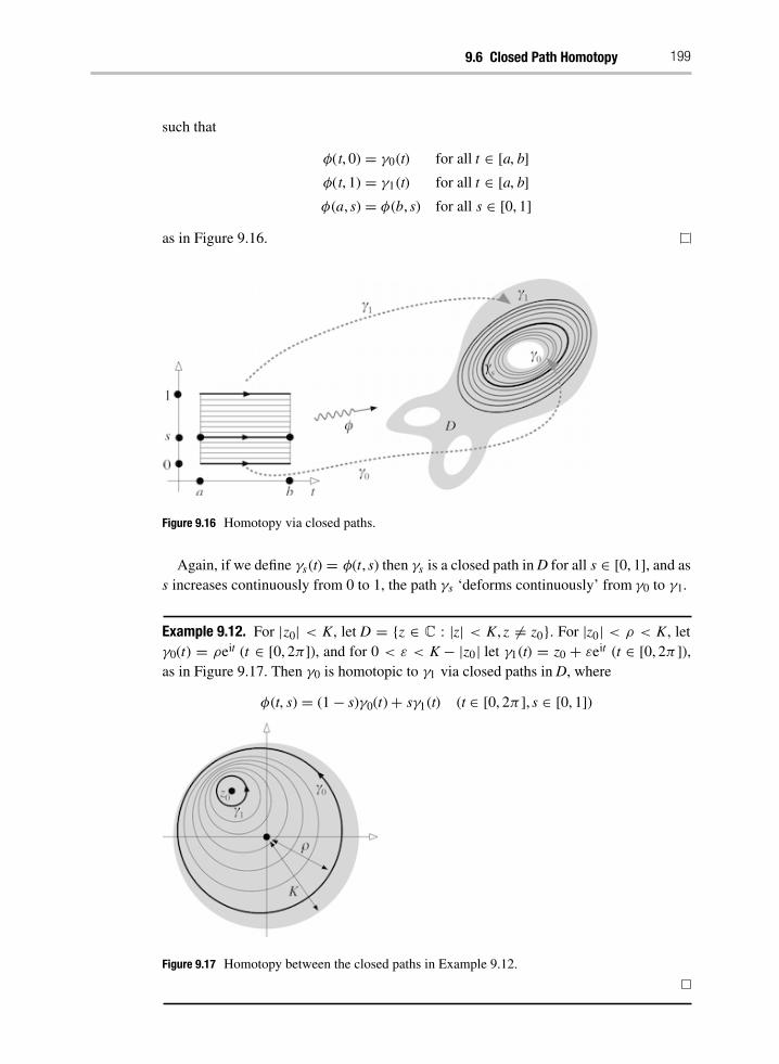
9.6 Closed Path Homotopy 199
such that
φ(t, 0) = γ0(t) for all t ∈ [a, b]
φ(t, 1) = γ1(t) for all t ∈ [a, b]
φ(a, s) = φ(b, s) for all s ∈ [0, 1]
as in Figure 9.16.
Figure 9.16 Homotopy via closed paths.
Again, if we define γs(t) = φ(t, s) then γs is a closed path inD for all s ∈ [0, 1], and ass increases continuously from 0 to 1, the path γs ‘deforms continuously’ from γ0 to γ1.
Example 9.12. For |z0| < K, let D = {z ∈ C : |z| < K, z ±= z0}. For |z0| < ρ < K, letγ0(t) = ρeit (t ∈ [0, 2π]), and for 0 < ε < K − |z0| let γ1(t) = z0 + εeit (t ∈ [0, 2π ]),as in Figure 9.17. Then γ0 is homotopic to γ1 via closed paths inD, where
φ(t, s) = (1− s)γ0(t)+ sγ1(t) (t ∈ [0, 2π ], s ∈ [0, 1])
Figure 9.17 Homotopy between the closed paths in Example 9.12.

200 Homotopy Versions of Cauchy’s Theorem
THEOREM 9.13. If f is differentiable in a domain D and closed paths γ0 , γ1 in D arehomotopic via closed paths in D, then
±γ0f =
±γ1f .
Proof. We have a continuous map φ : R→ D such that
φ(t, 0) = γ0(t) for all t ∈ [a, b]
φ(t, 1) = γ1(t) for all t ∈ [a, b]
φ(a, s) = φ(b, s) for all s ∈ [0, 1]
Let σ (s) = φ(a, s) (s ∈ [0, 1]). Then ∂φ = γ0 + σ − γ1 − σ (so σ is a cut from γ0 to γ1
in the sense of Section 8.7). By Cauchy’s Theorem for a boundary,²
∂φ
f =
²
γ0
f +
²
σ
f −
²
γ1
f −
²
σ
f = 0
so ²
γ0
f =
²
γ1
f
A closed path γ in D is homotopic to zero or null-homotopic if it is homotopic viaclosed paths in D to β : [a, b] → D where β(t) = z0 for all t ∈ [a, b], with z0 ∈ D. We
immediately deduce:
COROLLARY 9.14. Let f be differentiable in a domain D and let γ be a closed path inD that is homotopic to zero. Then
±γ f = 0.
The geometric significance of being homotopic to zero is that γ can be continuouslydeformed to a single point – more precisely, a path whose image is a single point – as inFigure 9.18.We can use a homotopy to prove that the interval of a differentiable complex function
is very well behaved under reparametrisation, of the path of integration. Here we canwork with merely continuous paths and parameter changes. For simplicity we do notchange the parametric interval. It is a useful exercise to include that possibility (intro-duce an affine map [a,b] → [c, d] and examine how that affects the integral). In thesmooth case it is also possible to use the formula for a change of variable in an integral.
Figure 9.18 A homotopy to zero.

9.7 Converse to Cauchy’s Theorem 201
PROPOSIT ION 9.15. Let f be differentiable on a domain D, and let λ : [a,b] → C be
a path in D. Let ρ : [a,b] → [a, b] be continuous, and let γ = λ ◦ ρ. Then±γ f =
±λ f .
Proof. Define a homotopy σ : [a, b] × [0, 1]→ D by
σ (t, s) = λ((1− s)t + sρ(t))
Clearly σs(t) ∈ D for t ∈ [a, b]. It is easy to check that
σ (t, 0) = γ
σ (t, 1) = λ
Therefore σ is a fixed end point homotopy from γ to λ. Now Theorem 9.10 applies.
9.7 Converse to Cauchy’s Theorem
Starting with Cauchy’s Theorem for a boundary we have deduced first the homotopy-
invariance of the integral for fixed end point or closed path homotopies, and then thatthe integral is zero for a path homotopic to zero. However, we can also start with Corol-lary 9.14 and argue the other way if we wish. First we need a simple result aboutchanging the parameter of a path:
PROPOSIT ION 9.16. Let γ : [a,b] → D be a path and let ρ : [a,b] → [a,b] be acontinuous map such that ρ(a) = a,ρ(b) = b. Then γ is homotopic to γ ◦ ρ.
Proof. Define φ : [a,b]× [0, 1]→D by
φ(t, s) = γ ((1− s)t + sρ(t))
This is a homotopy, and φ(t, 0) = γ (t),φ(t, 1) = γ (ρ(t)).
Note that the reparametrisation ρ is not required to be a bijection here. Also: all pathsγs have the same image. In effect we are performing a homotopy on the parameter.
We can now prove:
PROPOSIT ION 9.17. A closed path γ in D is a boundary ∂φ, up to reparametrisation,if and only if γ is homotopic to zero.
Proof. The need to reparametrise the interval on which γ is defined arises because of theway we have chosen a specific parametrisation for a boundary ∂φ. By Proposition 9.16we can adjust the parameter provided the images of γ and ∂φ coincide. This reduces theproof to a geometric argument. We give the essence of the proof in a series of pictures,leaving the reader the (routine) task of analytic definitions and verifications required tomake it rigorous.Define a map H : R → R, where R is a rectangle, as in Figure 9.19. The definition
proceeds in stages:
(1) Identify opposite vertical edges to get a cylinder.(2) Squash the top rim to a point to get a cone.

202 Homotopy Versions of Cauchy’s Theorem
Figure 9.19 Topological proof of Proposition 9.17.
(3) Open the cone out flat to get a disc.(4) Distort the disc to get a square.
Suppose that γ is a boundary, say γ = ∂φ where φ : R→ D. Then φ ◦H : R→ D is
a homotopy. The lower edge of R, marked by the heavy line in the first diagram, maps
to (the image under φ of ) ∂φ. The top edge maps to a point. So γ is homotopic to zero.Conversely, suppose that γ is a closed path homotopic to zero. Then we can define
a map of the cone into D such that the base circle goes to (the image of ) γ . Therefore(reversing the last two steps in the definition of H) we can map R into D so that itsperimeter goes to γ . Hence, up to reparametrisation, γ = ∂φ.
9.8 The Cauchy Theorems Compared
A common cause of distress for students of complex analysis is the sudden appearanceof a plague of Cauchy Theorems, having several variant hypotheses and a similar varietyof conclusions, but all begin derivable from each other. At times like this it may beadvisable to seek consolation elsewhere than mathematics: perhaps among the poets.Rudyard Kipling’s In the Neolithic Age makes the point admirably:
There are nine and sixty way of constructing tribal laysAnd – every – single – one – of – them – is – right!
It is much the same with the Cauchy Theorems: all of the different versions areessentially the same.
At the heart of all Cauchy-type theorems is the local existence of an antiderivative,Section 8.5. The theorems themselves supply, as hypotheses, conditions that permit thislocal result to be globalised in some way.

9.8 The Cauchy Theorems Compared 203
For example, in Chapter 8 the local result led to the central Cauchy Theorem 8.8, thatif f is differentiable in D and a closed contour does not wind round any point outside D,then
±γ f = 0. This ‘non-winding’ condition ensures that the local pieces of antideriva-
tive fit together well on the global level. The generalised version, with several contoursγ1, . . . ,γn, is a simple corollary obtained by making cuts between the contours.In this chapter we studied what happens when a contour is deformed continuously.
Again the local existence of an antiderivative is involved: it lets us define the integral off along an arbitrary path, and it gives the main result of that chapter, that the integral off along a boundary is zero. This is also a globalisation: associated with any boundary isa map of an entire rectangle, and the local antiderivatives all fit together properly acrossthe image of this rectangle. Moreover, we saw that a path is a boundary if and only if itis homotopic to zero. Since homotopy leaves the integral round a closed path invariant,this makes the reason why
±γ f = 0 transparent.
We therefore have two main variants of the Cauchy Theorem: one for paths that donot wind round points outside D, and another for paths that are homotopic to zero. But(more Kipling), like the Colonel’s Lady and Judy O’Grady, they are ‘sisters under theirskins’. Obviously if γ is homotopic to zero and z0 ±∈ D, then
w(γ , z0) =1
2π i
²
γ
1
z − z0dz = 0
because 1/(z − z0) is differentiable in D. So the ‘non-winding’ version of Cauchy’sTheorem easily implies the ‘homotopy’ version.It is in fact strictly stronger, in the following sense. The path in Figure 9.20 does not
wind round any z0 ±∈ D, but it is manifestly not homotopic to zero. (However, this isharder to prove than it might appear.) So the ‘non-winding’ hypothesis is weaker, henceapplies to more cases.Even this surface difference vanishes when we look a little more deeply, however.
Every path that does not wind round any z0 ±∈ D can be transformed, using a seriesof cuts whose contributions to the integral cancel, into a closed path (or set of paths)homotopic to zero. For example, Figure 9.20 (left) is so transformed in Figure 9.20(right). This fact is also non-trivial to prove, but it shows that the practical consequences
Figure 9.20 Left: A path that satisfies the non-winding condition but is not homotopic to zero.Right: Creating cuts in the path makes it homotopic to zero.

204 Homotopy Versions of Cauchy’s Theorem
of the extra generality are largely spurious. (The theoretical consequences are more
important: the ‘non-winding’ condition is part of ‘homology theory’, and what we havehere is a relation between homotopy and homology. We postpone a homology versionof Cauchy’s Theorem to Chapter 16, so that we can move on to more practical issues inChapters 10–14.)
9.9 Exercises
1. Let D = {z ∈ C : z ±= 0} and Sr(t) = reit (t ∈ [0, 2π]) for r = 1, 2. Define acontinuous map φ : R→ D, where R is a rectangle, such that
²
∂φ
f =²
S1
f −²
S2
f
for any f differentiable in D. Use Theorem 9.6 to deduce that²
S1
f =²
S2
f
Describe a homotopy via closed paths in D from S1 to S2.
2. Let γ1 ,γ2 be closed paths in a domain D that are homotopic via closed paths inD. By making a suitable cut σ from γ1 to γ2 , describe a fixed end point homo-
topy in D from γ1 to σ + γ2 − σ . Draw a picture to illustrate the continuousdeformation.
3. Let the boundary ∂φ of a continuous map φ : R → D be subdivided into twosubpaths ∂φ = γ1 + γ2. Describe a fixed end point homotopy in D from γ1 to −γ2 .Draw a picture to illustrate the continuous deformation.
4. Draw the semicircle γ (t) = eit (t ∈ [−π/2,π/2]) in D = C \ {0}. Define twoexplicit polygonal paths λ1, λ2 from −i to i in D such that
²
λ
f =²
γ
f
is true for all f differentiable in D when λ = λ1, but false when λ = λ2.
5. Let γ : [0, 1] →C be given by γ (0) = γ (1) = 0 and
γ (t) =´
t+ it sin(π/t) for t ∈ [0, 12]
(1− t) + i(1− t) sin(π/(1− t)) for t ∈ [ 12, 1]
Show that γ is a closed path but not a contour, and draw a sketch.
6. Integrate the following functions around the path γ in Exercise 5:(i) cos3(z2)
(ii)
∞³
n=1zn/n
(iii) 1/(z− 13
√2)

9.9 Exercises 205
7. Let f be differentiable in D. For a closed path γ in D, beginning and ending at z0 ,the integral value Iγ is the complex number
Iγ =
²
γ
f
Show that the set of integral values forms a commutative group I( f ,D) under theoperation
Iγ + Iδ = Iγ+δ
Determine the group of integral values in the following cases:(i) f (z) = 1/z,D = C \ {0}(ii) f (z) = cos z,D = C \ {0}(iii) f (z) = 2/(z− 1)+ 3/(z + 1),D = C \ {²1}(iv) f (z) = 1/(z− 1)+ 2/(z + 1),D = C \ {²1}
8. The Fundamental Group. Let D be a domain and z0 ∈ D. For closed paths γ , δ in D
that begin and end at z0 , define γ ³ δ to mean that γ , δ are fixed end point homo-
topic in D. Show that ³ is an equivalence relation. Let [γ ] denote the equivalenceclass containing γ , and let π(D, z0) be the set of equivalence classes.Define the operation ∗ on π (D, z0) by
[γ ] ∗ [δ] = [γ + δ]
Check that ∗ is well-defined, and show that π (D, z0) is a group under ∗, specifyingthe identity element and the inverse of [γ ].For any other point z1 ∈ D and any path σ in D from z0 to z1 , define g :
π(D, z0) → π(D, z1) byg([γ ]) = [−σ + γ + σ ]
Show that g is an isomorphism of groups and deduce that π (D, z0) is independentof the choice of z0 ∈ D. (This result relies on D being path-connected.) For thisreason, the group π (D, z0) is usually denoted by π(D) and called the fundamental
group of D.
9. Describe (without formal proof, since we have not developed suitable techniques)the fundamental groups of the following domains:
(i) C
(ii) {z ∈ C : |z| < 1}
(iii) {z ∈ C : |1 < z| < 2}
(iv) C \ {0}(v) C \ {²1}(vi) C \ Z
10. Let f be differentiable in the domain D, and let γ , δ be closed contours in D begin-
ning and ending at the same point z0 . Show that if γ ³ δ in the sense of Exercise 8,then the integral values Iγ and Iδ are equal. Prove that the map h : π (D)→ I( f ,D)
for which h([γ ]) = Iγ is a well-defined group homomorphism. Describe thehomomorphism h for each f in Exercise 7.

206 Homotopy Versions of Cauchy’s Theorem
11. Integrals Along Arbitrary Paths. For fixed z1, z2 ∈ D, suppose that γ0 is a fixed pathinD, and γ is a variable path inD, both from z1 to z2 . Show that
²
γ
f =
²
γ0
f + Iσ
for some σ ∈ I( f ,D). Prove that if γ is deformed continuously in a homotopy viaclosed paths in D, then Iσ remains constant.For z1 = −i, z2 = i, determine all possible values of
±γf for each f ,D in
Exercise 7.

10 Taylor Series
We now reach a stage in the theory were we can take a great leap forward and show,as promised repeatedly, that any differentiable complex function has a local powerseries representation. On the slim assumption that the derivative of f exists throughouta domain D, we find that near any point z0 ∈ D there is a power series expansion
f (z0 + h) =
∞±
n=0
anhn
for z0 + h ∈ Nr(z0)
which is valid – that is, converges – on any disc Nr(z0) ⊆ D, see Figure 10.1.
Figure 10.1 The power series round z0 converges on any disc in D.
This theorem releases a tidal wave of theorems, because we can apply the results ofChapter 4 on power series to any differentiable function f . For instance, Corollary 4.21states that a power series can be differentiated term by terms as many times as we like.Taylor’s Theorem, Corollary 4.22, gives an explicit formula:
f (z0 + h) =
∞±
n=0
f (n)(z0)
n!hn for z0 + h ∈ Nr(z0) ⊆ D
Thus if we insist only that the first derivative f ± exists in D, it follows that all higherderivatives exist, and the function is equal to its Taylor series in Nr(z0). We derive subtlerconsequences in this and subsequent chapters, and Cauchy’s Theorem plays a prominent
role. It is this sequence of results that gives complex analysis its own special flavour.

208 Taylor Series
Figure 10.2 Contours in the proof of the Cauchy Integral Formula.
10.1 Cauchy Integral Formula
The proof that any differentiable function can be expressed as a power series dependson a result of Cauchy, itself of intrinsic interest:
LEMMA 10.1 (Cauchy Integral Formula for a Circle). Let f be differentiable in the discNR(z0) = {z ∈ C : |z− z0| < R}. For 0 < r < R, let Cr be the path Cr(t) = z0+ reit (t ∈
[0, 2π]). Then for |w − z0| < r we have
f (w) =1
2πi
²
Cr
f (z)
z − wdz
Proof. Fix w such that |w − z0| < r. The function F(z) = ( f (z) − f (w))/(z − w) isdifferentiable in the domain
D = {z ∈ C : |z − z0| < R, z ²= w}
Let 0 < ε < r− |w − z0|. Then the circle Sε, centre w, radius ε, is
Sε(t) = z0 + εeit (t ∈ [0, 2π ])
and lies in D, as do all points inside Cr and outside Sε , see Figure 10.2.By the Generalised Cauchy Theorem, Theorem 8.9,
²
Cr
F(z)dz =
²
Sε
F(z)dz (10.1)
Now limz→w F(z) = f ±(w), so for some δ > 0,M ≥ 0, we have
0 < |z− w| < δ implies |F(z)| ≤ M
The Estimation Lemma, Lemma 6.41, implies that for ε < δ,³³³³²
Sε
F(z)dz
³³³³ ≤ M · 2πε

10.2 Taylor Series 209
From (10.1), ³³³³²
Cr
F(z)dz
³³³³ ≤ 2Mπε
Since ε is arbitrary, this implies that²
Cr
F(z)dz = 0
Therefore ²
Cr
f (z)
z− wdz =
²
Cr
f (w)
z− wdz
= f (w)
²
Cr
1
z− wdz
= f (w) · 2πi
In other words,
f (w) =1
2πi
²
Cr
f (z)
z − wdz
10.2 Taylor Series
Using the Cauchy Integral Formula we can now expand f (z0 +h) as a power series in h,with coefficients expressed as integrals.
LEMMA 10.2. Let f be differentiable in NR(z0).Then there exist an ∈ C such that
f (z0 + h) =
∞±
n=0
anhn
where the series converges absolutely for |h| < R. Further, if
Cr(t) = z0 + reit (t ∈ [0, 2π])
then
an =1
2πi
²
Cr
f (z)
(z − z0)n+1dz
Proof. Fix h with 0 < |h| < R and initially suppose that r satisfies |h| < r < R,
Figure 10.3.The Cauchy Integral Formula gives
f (z0 + h) =1
2π i
²
Cr
f (z)
z− (z0 + h)dz
=1
2π i
²
Cr
f (z)
´1
z− z0+
h
(z− z0)2+ · · · + hm
(z − z0)m+1
+hm+1
(z − z0)m+1(z− z0 − h)
µdz
=
m±
n=0
anhm + Am

210 Taylor Series
Figure 10.3 Contour for proof of Lemma 10.2.
where
an =1
2πi
²
Cr
f (z)
(z − z0)n+1dz
Am =1
2πi
²
Cr
f (z)hm+1
(z − z0)m+1(z − z0 − h)
dz
We demonstrate that limm→∞ Am = 0.
First, since f is differentiable it is continuous, so φ(t) = | f (Cr(t))| is a continuous realfunction on [0, 2π ]. From real analysis, φ is bounded, so
|φ(t)| ≤ M for z on Cr
Now |h| < r, |z− z0| = r, and
|z− z0 − h| ≥ ||z− z0| − |h|| = r − |h|
Therefore the Estimation Lemma gives
|Am | ≤1
2π
M|h|m+1
rm+1(r − |h|)2πr =
M |h|
r− |h|
¶|h|
r
·m
Since we chose |h| < r, this tends to zero as m tends to infinity. Thus
limm→∞
¸f (z0 + h)−
m±
n=0
anhn
¹= 0
which means that
f (z0 + h) =
∞±
n=0
anhn
This expansion is valid for |h| < R, and
an =1
2πi
²
Cr
f (z)
(z − z0)n+1
dz

10.2 Taylor Series 211
for |h| < r. The latter restriction can now be seen to be unnecessary, for the integral isdifferentiable for 0 < |z−z0| < R, so the integral is unchanged if r is varied in the range0 < r < R.
Once we know that a power series expansion exists, we can use our knowledge ofpower series to deduce:
THEOREM 10.3 (Taylor Series). If f is differentiable in a domain D, then all higherderivatives of f exist throughout D. In any disc NR(z0) ⊆ D the Taylor series expansion
f (z0 + h) =
∞±
n=0
f (n)(z0)
n!hn (10.2)
is valid. Further, if 0 < r < R and Cr(t) = z0+ reit (t ∈ [0, 2π ]), then
f (n)(z0) =n!
2π i
²
Cr
f (z)
(z− z0)n+1dz
Proof. From Lemma 10.2,
f (z0 + h) =
∞±
n=0
anhn for |h| < R
In other words, putting z = z0+ h,
f (z) =
∞±
n=0
an(z− z0)n for |z − z0| < R
Now, a power series may be differentiated term by term as often as we please, and byCorollary 4.22
f(n)(z0) = n!an =
n!
2π i
²
Cr
f (z)
(z− z0)n+1
dz
This gives the desired integral expression for f (n)(z0). Substituting an = ( f (n)(z0))/n! inthe power series gives the Taylor expansion.
Theorem 10.3 was first proved by Cauchy in 1831 by the method above. The series isnamed after Brooke Taylor, who in 1715 was the first to publish the idea that a functioncan be expanded as a power series of the form
f (x+ h) =
∞±
n=0
f (n)(x)
n!hn
Taylor’s theory was restricted to real functions, and it will come as no surprise that theidea was previously known to others; specifically to James Gregory, who was aware of itsome 45 years earlier, and to Newton in 1691. During the eighteenth century there werevarious attempts to base the theory of real analysis on power series, the most famousbeing that of Joseph-Louis Lagrange in 1797. Cauchy used power series extensively incomplex analysis. It is a curious quirk of fate that in 1829 he quoted the counterexamplef (x) = e−1/x
2to show that not every infinitely differentiable real function is equal to

212 Taylor Series
its Taylor series. Just two years later he went on to show that all differentiable complexfunctions have valid power series expansions.We now introduce some standard terminology, which until now we have avoided.
DEFIN IT ION 10.4. A real function f : D → R, where D ⊆ R, or a complex functionf : D→ C, where D ⊆ C, is analytic if for each α ∈ D it has a power series expansion
f (α + h) =
∞±
N=0
anhn
valid in some neighbourhood of α.
Cauchy demonstrated that in the real case there are functions that are infinitely dif-ferentiable but not analytic. But in the complex case he proved that any function thatis differentiable once in a domain must be analytic. At a stroke he showed that in thisrespect complex analysis is simpler than real analysis, and reduced the general study ofdifferentiable complex functions to computations with power series, giving the sequenceof theorems that unfolds in the next few sections.REMARK 10.5. A complex function on a domain is differentiable if and only if it is ana-lytic. The two words just emphasise different points of view – existence of a derivative,existence of a power series expansion – and may be used interchangeably.
10.3 Morera’s Theorem
First we have a partial converse to Cauchy’s Theorem, due to Giacinto Morera in 1889:
THEOREM 10.6 (Morera’s Theorem). If f : D → C is continuous in a domain D andºγf = 0 for all closed contours γ in D, then f is differentiable in D.
Proof. By Theorem 6.44, ifºγf = 0 for all closed contours γ in D, then there exists a
differentiable function F in D whose derivative is f . But now we know that F is twice(indeed infinitely) differentiable, so f = F± is differentiable.
This theorem explains our warning in Chapter 6 that it is futile to try to find anantiderivative F for a non-differentiable complex function f . It cannot have one. So thereis a class of functions, including f (z) = |z|, that are continuous but not differentiable.Such functions are integrable, via the formula
²
γ
f =
² b
a
f (γ (t))γ ±(t)dt
but the Fundamental Theorem of Contour Integration is no use whatsoever in this con-text, because f has no antiderivative – in stark contrast to the real case, where everycontinuous function has an antiderivative. (It can be argued that here real analysis issimpler than complex.)To summarise what we know about the existence of derivatives and antiderivatives
for complex functions:

10.4 Cauchy’s Estimate 213
If f is differentiable in a domain D, then all higher derivatives of f exist. The func-tion f has an antiderivative only when f is differentiable, and even then, only local
antiderivatives are guaranteed. Specifically, if D1 ⊆ D is simply connected, then f has
an antiderivative in D1, Theorem 8.12. In particular, we can guarantee the existence ofan antiderivative of a differentiable function in any disc contained in its domain.
10.4 Cauchy’s Estimate
Theorem 10.3 includes a generalisation of Cauchy’s Integral Formula to the higherderivatives of a differentiable function:
f (n)(z0) =n!
2π i
²
Cr
f (z)
(z− z0)n+1dz
where NR(z0) ⊆ D and 0 < r < R. With the standard conventions that f (0)(z) = f (z) and0! = 1, this formula is true for all integers n ≥ 0. Using it, we can give an upper boundfor | f (n)(z0)|:
LEMMA 10.7 (Cauchy’s Estimate). If f : D → C is differentiable for z− z0 < R,
0 < r < R, and | f (z)| ≤ M for |z− z0| < r, then
| f(n)(z0)| ≤
Mn!
rn
Proof.
| f(n)(z0)| =
³³³³n!
2πi
²
Cr
f (z)
(z− z0)n+1
dz
³³³³
≤n!
2π
M
rn+1· 2πr
=Mn!
rn
Cauchy’s Estimate yields an important theorem of Joseph Liouville, which has anunexpected application to a purely algebraic problem:
THEOREM 10.8 (Liouville’s Theorem). If f is differentiable and bounded in the wholecomplex plane, then f is constant.
Proof. Suppose that | f (z)| ≤ M for all z ∈ C. Cauchy’s Estimate applied to thederivative gives
| f ±(z)| ≤M
r
Since f is differentiable on C we may let r → ∞, making M/r as small as we please.Since | f ±(z)| is independent of r, we have
f ±(z) = 0
Thus f ±(z) = 0 throughout C, and (integrating) f is constant.
The application is:

214 Taylor Series
THEOREM 10.9 (Fundamental Theorem of Algebra). Let P(z) = zn+a1zn−1+· · ·+an
be a polynomial, where n ≥ 1 and a1, . . . ,an ∈ C. Then there exists w ∈ C with
P(w) = 0.
Proof. For a contradiction, suppose that P(z) ²= 0 for all z ∈ C. Then 1/P(z) isdifferentiable throughout C.Suppose z ²= 0. Then
P(z)
zn= 1+
a1
z+ · · · + an
zn→ 1 as |z| → ∞
So there exists k > 0 such that³³³³P(z)
zn
³³³³ ≥12
for |z| > k
Thus ³³³³1
P(z)
³³³³ ≤2
|zn|≤
2
knfor |z| > k
The same bound works for 1/P(z) throughout C. For if z ≤ k we take a circle CR centre
z0 , radius R, which is so large that |z| > k for all z on CR. Then³³³³1
P(z)
³³³³ ≤2
knfor all z on CR
and Cauchy’s Estimate gives ³³³³1
P(z)
³³³³ ≤2
kn
By Liouville’s Theorem, 1/P(z) is constant, so P(z) is constant. But this contradictsn ≥ 1. Therefore P(w) = 0 for somew ∈ C.
It follows in the usual way that any polynomial P(z) of degree n, with complex
coefficients, can be expressed as a produce of terms of degree 1:
P(z) = (z − α1)(z − α2) · · · (z− αn)
where the αj ∈ C.
10.5 Zeros
We now broaden our perspective from polynomials, and look at the zeros of arbitrarydifferentiable functions.
DEFIN IT ION 10.10. A zero of a differentiable function f : D → C is a point z0 ∈ D
for which f (z0) = 0.
Expanding f in a Taylor series about the zero z0 , we have
f (z) =
∞±
n=0
an(z− z0)n for |z − z0| < R

10.5 Zeros 215
where NR(z0) ⊆ D. Then a0 = f (z0) = 0, and two distinctly different things can occur:either all of the other am are zero, in which case f (z) = 0 for all z ∈ NR(z0), or thereexists m ≥ 1 such that
a0 = a1 = · · · = am−1 = 0, but am ²= 0 (10.3)
DEFIN IT ION 10.11. If (10.3) holds, then z0 is a zero of order m, or a zero of finite orderif m is unspecified.
The notion of a zero of order m relates directly to that of an infinitesimal of order min Chapter 15.Formula (10.2) for the Taylor coefficients implies that a zero of order m can be
characterised by the condition
f (z0) = f ±(z0) = · · · = f (m−1)(z0) = 0, but f (m)(z0) ²= 0
Another useful expression for such a zero is to write
f (z0) = (z − z0)mg(z) (|z− z0| < R)
where
g(z) =
∞±
n=0
am+n(z− z0)n
is differentiable for |z − z0| < R and g(z0) = am ²= 0.
This leads to a fundamentally important idea:
DEFIN IT ION 10.12. A zero z0 of a differentiable function f : D → C is isolated if
some disc centred upon it contains no other zeros of f ; that is, there exists δ > 0 suchthat
0 < |z− z0| < δ implies f (z) ²= 0
LEMMA 10.13. A zero of finite order is isolated.
Proof. Write f (z0) = (z − z0)mg(z) for |z − z0| < R, where g is differentiable and
g(z0) ²= 0. Then g is continuous at z0 , so, taking ε = 12|g(z0)| there exists δ > 0 such
that
|z− z0| < δ implies |g(z) − g(z0)| < ε
Therefore, when |z− z0| < δ we have
|g(z)| ≥ ||g(z0)| − |g(z0) − g(z)|| > 2ε − ε = ε
In particular, g(z) ²= 0. But if 0 < |z − z0| < δ then |z − z0|m ²= 0, so f (z) = (z − z0)
m
g(z) ²= 0.
COROLLARY 10.14. Let S be a set of zeros of a differentiable function f in D, havinga limit point z0 ∈ D. Then f is identically zero in any disc NR(z0) ⊆ D.

216 Taylor Series
Proof. Because z0 is a limit point of S, there is a sequence {zn}n≥1 in S that tends to z0 .Then f (z0) = limn→∞ f (zn) = 0. So z0 is a zero of f that is not isolated. Hence it doesnot have finite order, so
f (z0 + h) =
∞±
n=0
anhn
in any disc NR(z0) ⊆ D, where all an are zero.
From this we deduce:
PROPOSIT ION 10.15. If f is differentiable in a domain D and S is a set of zeros of fwith a limit point z0 ∈ D, then f is identically zero on D.
Proof. Corollary 10.14 gives f (z) = 0 for z in any disc NR(z0) ⊆ D.
For any other z ∈ D, choose a path γ : [a,b]→ D from z0 to z, Figure 10.4. We showthat f (γ (t)) = 0 for all t ∈ [a,b]. By continuity, we can find δ > 0 such that
a ≤ t < a+ δ implies γ (t) ∈ NR(z0)
so f (γ (t)) = 0 for a ≤ t < a+ δ. Let s be the least upper bound of those x ∈ [a,b] suchthat f (γ (x)) = 0 for a≤ t < x. Then a+ δ ≤ s ≤ b.
By continuity, f (γ (s)) = 0. If s < b then γ (s) is a non-isolated zero, so f is identicallyzero in a neighbourhood of γ (s). Then there exists an interval [s, s+ κ] with κ > s, onwhich f (γ (t)) = 0, contradicting the definition of s. Hence s = b, so f (z) = f (γ (b)) =
0.
An important consequence is:
THEOREM 10.16 (Identity Theorem). If f and g are differentiable in a domain D andf (z) = g(z) for all z ∈ S ⊆ D where S has a limit point in D, then f = g throughout D.
Proof. Apply Proposition 10.15 to f − g.
Figure 10.4 Proof of Proposition 10.15.

10.6 Extension Functions 217
Example 10.17. It is essential for the relevant limit point of S to be in D: if not, thetheorem can be false. Let
f (z) = sin(1/z)
g(z) = 0
in D = C \ {0}. Then f (z) = g(z) for z = ³1/(nπ ) and z0 = 0 is a limit point ofS = {³1/(nπ )}, but f ²= g inD.
10.6 Extension Functions
Combining the Identity Theorem with power series leads to a method that can oftenextend the domain of definition of a complex differentiable function.
DEFIN IT ION 10.18. A function f : D → C is an extension function of h : S → C if
S ⊆ D and f (z) = h(z) for all z ∈ S. (We also say that f extends h.)
Example 10.19. f (z) = 1/(1 − z) on D = C \ {1} is an extension function of h(z) =∑∞
n=0 zn on S = {z ∈ C : |z| < 1}.
Suppose that D is a domain and S ⊆ D has a limit point in D. The Identity Theoremshows that if a function f : S → C has a differentiable extension function g : D ⊆ C,
then the extension is unique.As an application, suppose that f : D → C is differentiable and consider the Taylor
expansion f (z) =∑∞
n=0 an(z − z0)n of f in a disc Nr(z0) ⊆ D. Then f is the only
possible extension of the Taylor expansion to the whole of D. This means that althoughthe Taylor expansion may not converge on the whole of D, it contains all the information
needed to determine f uniquely throughout D. We use this fact to great advantage inChapter 14.
Example 10.20. Consider the power series
z−z2
2+ · · · + (−1)
n zn
n+ · · · (10.4)
on the small disc S = {z ∈ C : |z| < 1/1 000 000}. We can certainly extend this functionto a larger disc, because the radius of convergence of the power series is 1. However,we can extend beyond this. For instance, if K = {t ∈ R : t ≤ −1} and D = C \ K,
then f (z) = log(1 + z) is the (unique) differentiable extension of the power series to D,
Figure 10.5.

218 Taylor Series
Figure 10.5 Extending the power series (10.4) toC \ K.
The set S need not be a domain. In particular, it may be a subset of R:
Example 10.21. f (z) = sin z for z ∈ C is the unique differentiable extension function off (x) = sin x for x ∈ R. This is a consequence of the usual convergent Taylor expansionin the real case.
Of course, if D is a domain then it is open, so D ∩ R is open in R. A differentiablefunction f : D→ C has a power series expansion in a neighbourhood of any x0 ∈ D∩R.
So if a real function h : S → R extends to a differentiable complex function on adomain, it must already have a power series expansion about any point in S ⊆ D ∩ R.
Thus the only real functions that extend to differentiable complex functions are realanalytic functions.
We may take S to be even more restricted, provided that it has at least one limit pointin D:
Example 10.22. If f (1/n) = 1/n2 for all positive integers n, then f (z) = z2 is the uniqueanalytic extension of f to the whole complex plane, because
S = {1/n : n is a positive integer}
has the limit point 0 ∈ C.
The Taylor expansion is valid on discs (Theorem 10.3), and may therefore be used todefine extension functions. It is therefore easy to see that the radius of convergence ofthe Taylor expansion of a function f about a point z0 is equal to the distance from z0 to
the nearest point z1 at which no differentiable extension function of f may be defined.Such a point is called a singularity of f , see Chapter 11. Singularities are obstacles thatdetermine the radius of convergence of a Taylor series.(There is no relation between this use of ‘singularity’ and the term ‘singu-
lar’ in Definition 6.20. ‘Singular’ is just one of those words that get overused inmathematics.)

10.7 Local Maxima and Minima 219
10.7 Local Maxima and Minima
The complex numbers are not ordered, so we cannot speak of maxima and minima of acomplex function f . We can, however, consider maximum and minimum values of themodulus | f |, since this is real.
DEFIN IT ION 10.23. If f : D → C, then
(i) The modulus | f | has a local maximum at z0 ∈ D if there exists ε > 0 such thatNε(z0) ⊆ D and | f (z)| ≤ | f (z0)| for all z ∈ N
ε(z0). The local maximum is strict if
| f (z)| < | f (z0)| for all z ∈ Nε (z0) \ {z0}.(ii) The modulus | f | has a local minimum at z0 ∈ D if there exists ε > 0 such that
Nε(z0) ⊆ D and | f (z)| ≥ | f (z0)| for all z ∈ Nε(z0). The local minimum is strict if| f (z)| > | f (z0)| for all z ∈ N
ε(z0) \ {z0}.
The problem of finding local maxima of | f | in a domain turns out to be easy (orimpossible, depending on how you look at it, since there are none.)
PROPOSIT ION 10.24. A differentiable function has no strict local maximum of itsmodulus in its domain. If it has a local maximum in its domain, it is constant.
Proof. Suppose that f is differentiable in D and let z0 be a local maximum in D. Then| f (z)| ≤ | f (z0)| for all z ∈ Nε (z0). For 0 < r < ε, the circleCr(t) = z0+re
it (t ∈ [0, 2π ])lies inside Nε(z0), so | f (z0 + reit)| ≤ | f (z0)| for all t ∈ [0, 2π ]. The Cauchy Integralformula gives
f (z0) =1
2π i
²
Cr
f (z)
z− z0dz
=1
2π i
² 2π
0
f (z0 + reit )
reitireitdt
=1
2π i
² 2π
0
f (z0 + reit)dt
so that
| f (z0)| ≤1
2π
² 2π
0
| f (z0 + reit)|dt ≤1
2π
² 2π
0
| f (z0)|dt ≤ | f (z0)|
Hence
| f (z0)| =1
2π
² 2π
0
| f (z0 + reit)|dt (10.5)
If the strict inequality | f (z0 + reit)| < | f (z0)| were to hold for any t ∈ [0, 2π ], then bycontinuity it would also hold in a small interval, giving the strict inequality
1
2π
² 2π
0
| f (z0+ reit)|dt < | f (z0)|
contradicting (10.5).

220 Taylor Series
Hence | f (z0 + reit)| = | f (z0)| for all t ∈ [0, 2π]. This holds for any r < ε , so | f | isconstant in Nε(z0). By Proposition 4.15, f is constant in Nε(z0). The Identity Theoremnow shows that f is constant throughout D.
For the complementary notion of a local minimum of | f |, it is clear that if f is non-constant and has a zero at z0 then z0 is isolated and | f | has a strict local minimum
there. If f is non-zero on D, observe that | f | has a strict local minimum if and only if|1/f | = 1/| f | has a strict local maximum. We can apply Proposition 10.24 to 1/f to get:
PROPOSIT ION 10.25. A differentiable function that does not equal zero anywhere inits domain has no strict local minimum of its modulus in its domain. If it has a localminimum in its domain, it is constant.
10.8 The Maximum Modulus Theorem
The question of maxima or minima of | f | on an arbitrary subset of the domain of f issomewhat different.
DEFIN IT ION 10.26. Let f : D → C be differentiable in a domain D, and let S ⊆ D.
Then | f | has a local maximum on S at z0 ∈ S if
(i) z0 is a limit point of S.(ii) For some ε > 0, | f (z)| < | f (z0)| whenever z ∈ Nε (z0) ∩ S.
Condition (i) is essential, for otherwise some neighbourhood Nε(z0) contains nopoints of S other than z0 , and then condition (ii) is vacuously true.
Example 10.27. If f (z) = ez and S = {z ∈ C : |z| ≤ 1}, then | f (x+ iy)| = ex and | f | has
a local maximum on S at the point z0 = 1.
Using Proposition 10.24, we see that if Nε (z0) ⊆ S, then | f | cannot have a strict localmaximum at z0 . To explore this further, we need:
DEFIN IT ION 10.28. A point z0 is a boundary point of S if every neighbourhood of z0contains a point in S and a point not in S, other than z0 itself. In other words, a boundarypoint is a limit point both of S and its complement C \ S.
The boundary ∂S of S is its set of boundary points.
Example 10.29. The boundary of S = {z ∈ C : |z| ≤ 1} and of of its complement
{z ∈ C : |z| > 1} is the circle {z ∈ C : |z| = 1}.
We can now rephrase Proposition 10.24 to give:

10.9 Exercises 221
THEOREM 10.30 (Maximum Modulus Theorem). If a differentiable function is notconstant, then any local maximum value of its modulus on an arbitrary subset of itsdomain occurs on the boundary of that set.
We also have from Proposition 10.25:
THEOREM 10.31 (Minimum Modulus Theorem). If a differentiable function is not con-stant, then any local minimum value of its modulus on an arbitrary subset of its domainoccurs either at a zero of the function, or on the boundary of that set.
Example 10.32. If f (z) = z2 on the set S = {z ∈ C : |z| ≤ 1}, then the maximum valuesof | f (x + iy)| = x2 + y2 occur all round the boundary of S, while the minimum valueoccurs at the origin.
10.9 Exercises
1. Find the Taylor series at 0 of f (z) = Log(1 + z), where Log is the principalvalue. What is the disc of convergence? Answer the same questions for g(z) =exp(αLog(1 + z)), where α ∈ C.
2. Find the first three terms and radius of convergence for the Taylor series at 0 ofF(z) = [1+ Log (1− z)]−1.
3. Taylor expand the following functions around 0, and find the radius of convergence.(i) sin2 z(ii) z2(z+ 2)−2
(iii) (az+ b)−1 (a, b ∈ C, b ²= 0)
(iv)º z
0exp(w2)dw
(v)
´(sin z)/z (z ²= 0)
1 (z = 0)
(vi)º z
0(sinw)/w dw
4. Define the numbers cn by the Taylor series
sec z =
∞±
n=0
(−1)nc2n
(2n)!z2n
Prove that
c0 = 1
0 = c0 + c2
¶2n
2
·+ c4
¶2n
4
·+ · · · + c2n
¶2n
2n
·
Show that c2n is always an integer and calculate it for n ≤ 5.
5. Let(1− z− z2)−1 =
±Fnz
n

222 Taylor Series
Prove thatF0 = F1 = 1 Fn = Fn−1 + Fn−2 (n ≥ 2)
This is the recursive definition of the Fibonacci numbers 1, 1, 2, 3, 5, 8, 13, . . ..By expanding (1 − z− z2)−1 in partial fractions, prove that
Fn =1√5
⎡
⎣¸1+
√5
2
¹n+1−¸1−
√5
2
¹n+1⎤
⎦
6. Investigate analogous results to Exercise 5 on the expansion of (1 − az− bz2)−1 ,for a,b ∈ C.
7. If
exp
¶z
1− z
·=±
anzn
prove that
a0 = 1 an =n±
s=1
1
s!
¶n− 1s− 1
·
8. Let f (z) have Taylor series∑
anzn for |z| < R. Let ω = e2π i/3 and define
g(z) = 13 ( f (z)+ f (ωz) + f (ω2z))
Show thatg(z) =
±a3nz
3n
for |z| < R. Find similar expressions for∑
a3n+1z3n+1 and∑
a3n+2z3n+2 . (Hint:1+ ω + ω2 = 0.)
9. Define three functions by
α(z) =± z3n
(3n)!β(z) =
± z3n+2
(3n+ 2)!γ (z) =
± z3n+1
(3n+ 1)!Prove the series converge for all z. Using Exercise 8, prove the following:(i) α±(z) = β(z) β±(z) = γ (z) γ ±(x) = α(z)
(ii) α(z) = 13[e
z + 2e−z/2 cos(z√3/2)]; find similar expressions for β(z), γ (z).
(iii) α(z + w) = α(z)α(w) + β(z)γ (w) + γ (z)β(w)
(iv) α3(z)+ β3(z)+ γ 3(z) = 1
(v) α(z) = β(z) ⇐⇒ z = (3n− 1) · 2π3√3(n ∈ Z)
10. Generalise Exercise 8 to find an expression for∑
apnzpn (p = 2, 3, . . .), and (harder)
for∑
apn+kzpn+k (p = 2, 3, . . . ;k = 0, 1, . . . ,p− 1).11. Show that the Cauchy estimate is an equality if and only if f (z) = Kzn for some
K ∈ C, n = 1, 2, 3, . . ..12. Let D be a disc centre z0 , and let f be differentiable in a domain containing D.
Prove that the ‘mean value’ of f (z) as z runs over ∂D (defined by a suitable integral)is equal to f (z0).

10.9 Exercises 223
13. Let f be differentiable throughout C, and suppose that | f (z)| ≤ K|z|c for a realconstant K and positive integer c. Prove that f is a polynomial function of degree≤ c.
14. Let f and g be differentiable on the strip D = {z ∈ C : −2 < im z < 2}. Supposethat f (z) = g(z) for all z such that |z| < 0.01. By considering Taylor expansions firstabout 0, then 1, and so on by induction, prove that f (z) = g(z) on D.
15. Suppose that f (z) =∑
an(z − z0)n in a disc D centre z0, radius R. If 0 ≤ r < R,
show that1
2π
² 2
0
| f (z0 + reiθ )|2dθ =±
|an|2r2n
(Parseval’s Inequality). Hence show that±
|an|2r2n ≤M(r) = sup
θ
| f (z0 + reiθ )|
Use this to give an alternative proof of the Maximum Modulus Theorem.
16. If p(z) is a polynomial of degree n, show that for each R > 0 the ‘level curve’ of|p(z)|, defined to be {z ∈ C : |p(z)| = R}, has at most n connected components.
17. Suppose that x2+ y2 ≤ a2 . Prove that (1+x)2+ y2 attains its maximum value whenx = a, y = 0. (Hint: apply the Maximum Modulus Theorem to 1 + z on the disc|z| = a.)
18. Suppose that x2 + y2 ≤ 1. Prove that (x2 − y2 − 1)2 + 4x2y2 attains its maximum
value when x = 0, y = ³1.19. If f is differentiable in a domain D, prove that the zeros of f are either all of finite
order and isolated, or f is identically zero on D.
20. Let
f (x) =
²∞
x
t−1ex−tdt
where x is real and positive. By repeated integration by parts, show that if
hn(x) = (−1)nn!x−(n+1)
then
f (x) = h0(x)+ h1(x)+ · · · + hn−1(x) + (−1)n² ∞
x
ext−(n+1)dt
Show that the series∞±
n=0
hn(x) (10.6)
diverges for all x. Show also that³³³³³ f (x)−
N±
n=o
hn(x)
³³³³³ < N!x−(N+1)

224 Taylor Series
so that for large enough x the series (10.6) provides an arbitrarily good approxima-
tion to f (x), even though it diverges.(The catch is that, the better the approximation required, the larger x has to be.
No particular choice of x gives an arbitrarily good approximation if we take N large
enough. A series with this property is called an asymptotic series.)
11 Laurent Series
The Taylor series expansion is too limited for many applications. A useful generalisationwas given by Laurent in 1843. Weierstrass may have discovered it two years earlier, buthis paper was not published until after his death. Laurent considered ‘power series’involving negative powers as well as positive. The benefits that accrue are hinted at bythe following example. The function f (z) = e−1/z
2is very badly behaved as regards
Taylor series expansion. We have seen that, restricted to the real line, its Taylor seriesabout the origin is 0+0x+ 0x2+ · · · , which does not converge to f (x). On the complex
plane it is, if such a statement makes sense, even less capable of being represented bya Taylor series. The natural series representation is obtained by starting with the Taylorseries for ez and replacing z by −1/z2, giving
f (z) = 1− z−2+
1
2!z−4+
1
3!z−6+ · · ·
and this is a series of the ‘negative powers’ type. It converges for all z for which −1/z2is defined, namely z ±= 0.
11.1 Series Involving Negative Powers
The general series of this type can be written in the form∞±
n=−∞
an(z − z0)n
which is to be thought of as a compact notation for²∞±
n=0
an(z − z0)n
³+
²∞±
n=1
a−n(z− z0)−n
³
and hence converges if and only if the two series in parentheses converge. We know thatpower series converge inside a disc. Consequently power series with negative powersalone should converge outside a disc. For instance, that for e−1/z2 converges outside thedisc |z| = 0. Therefore those with both positive and negative powers should converge ina region between two concentric circles. Recall that such a region is called an annulus.More precisely, if R1, R2 ∈ Rwith 0 ≤ R1 < R2 ≤ ∞, and z0 ∈ C, then
{z ∈ C : R1 ≤ |z − z0| ≤ R2}

226 Laurent Series
is an annulus.We begin with an existence theorem for series expansions of the above kind.
THEOREM 11.1 (Laurent’s Theorem). If f is differentiable in the annulus R1 ≤ |z −z0| ≤ R2 where 0 ≤ R1 < R2 ≤ ∞, then
f (z0 + h) =
∞±
n=0
anhn+
∞±
n=1
bnh−n
where∑
anhn converges for |h| < R2 ,
∑bnh
−n converges for |h| > R1 , and inparticular both sides converge in the interior of the annulus.Further, if Cr(t) = z0 + reit, (t ∈ [0, 2π ]) then
an =1
2π i
´
Cr
f (z)
(z− z0)n+1
dz
bn =1
2π i
´
Cr
f (z)(z− z0)n−1dz
Before giving the proof:REMARK 11.2. In the more compact notation we set cn = an (n ≥ 0) and c−n = bn
(n ≥ 1). Then
f (z0 + h) =
∞±
n=−∞
cnhn
which converges in the interior of the annulus, and
cn =1
2π i
´
Cr
f (z)
(z− z0)n+1
dz
for all n ∈ Z.
Proof of Theorem 11.1. If R1 < |h| < R2 , choose r1 , r2 such that
R1 < r1 < |h| < r2 < R2
and let
Cr1 (t) = z0 + r1eit (t ∈ [0, 2π])
Cr2 (t) = z0 + r2eit (t ∈ [0, 2π])
as in Figure 11.1.We show first that
f (z0 + h) =1
2π i
´
Cr1
f (z)
(z− (z0 + h))dz−
1
2π i
´
Cr2
f (z)
(z− (z0 + h))dz (11.1)
To do so, enclose z0 + h in a small circle
Sε(t) = z0 + εeit (t ∈ [0, 2π ])
Then the function
F(z) =f (z)
z − (z0 + h)

11.1 Series Involving Negative Powers 227
Figure 11.1 An annulus, showing paths used to prove Theorem 11.1.
is differentiable in
S= {z ∈ C : R1 < |z − z0| < R2 , z ±= z0 + h}
and the contours −Cr2 , Cr1 , Sε satisfy the hypotheses of Theorem 8.9. Therefore´
−Cr2
F(z)dz+
´
Cr1
F(z)dz+
´
Sε
F(z)dz = 0
Hence´
Sε
F(z)dz =
´
Cr2
F(z)dz−
´
Cr1
F(z)dz
But by Cauchy’s Integral Formula,
´
Sε
F(z)dz = 2π i · f (z0 + h)
giving (11.1).(Alternatively we can make cuts and integrate round the two halves, as shown in
Figure 11.2. The parts of the contours along the cuts cancel in pairs when integrated.)All we need do now is work out the two integrals in (11.1) as power series, and
calculate the coefficients. Unfortunately this is the longer part of the proof, although thecalculations are routine.First, we choose ρ1, ρ2 with
r1 < ρ1 < |h| < ρ2 < r2
which enforces the conditions:
(i) |z− (z0 + h)| > r2 − ρ2 for z on Cr2 ; and(ii) |z− (z0 + h)| > ρ1 − r1 for z on Cr1 .

228 Laurent Series
Figure 11.2 Alternative proof using cuts.
As in the proof of the Taylor series expansion, Lemma 10.2, we get
1
2π i
´
Cr1
f (z)
z− (z0 + h)dz =
∞±
n=0
anhn
for |h| < ρ2, where
an =1
2π i
´
Cr1
f (z)
(z− z0)n+1
dz
The treatment of the second integral is similar, but will be given in full. Since
1
h+
z− z0
h2+ · · · +
(z− z0)n−1
hn−
(z− z0)n
hn(z− z0 − h)=
−1
z− z0 − h
(summing a geometric series) we have
−1
2πi
´
Cr2
f (z)
(z − z0 − h)dz =
1
2π i
´
Cr2
f (z)
µ1
h+ · · · + (z − z0)
n−1
hn−
(z− z0)n
hn(z− z0 − h)
¶dz
=
n±
m=1
bmh−m− Bn
where
bm =1
2πi
´
Cr2
f (z)(z− z0)m−1dz
Bn =1
2πi
´
Cr2
f (z)(z− z0)n
hn(z− z0 − h)
Finally we estimate the size of Bn . There exists M > 0 such that | f (z)| ≤ M on Cr1
since this circle is closed and bounded. By (i) above, |z − z0 − h| > ρ1 − r1 . Also|h| > ρ1 , |z − z0| = r1. Hence
|Bn| ≤1
2π
Mrn1
ρn1(ρ1 − r1)
· 2π r1 =Mr1
ρ1 − r1
·r1
ρ1
¸n

11.1 Series Involving Negative Powers 229
which tends to 0 as b= n→ ∞, since r1/ρ1 < 1. It follows that
−1
2π i
´
Cr2
f (z)
(z− z0 − h)dz =
∞±
m=1
bmh−m
To finish the proof we must replace Cr1 and Cr2 by Cr in the expressions for an and
bn. Since all three paths are homotopic inside the annulus, or by using cuts, this isimmediate.
Note that we can no longer assert that an = f (n)(z0)/n! since f (z) need not bedifferentiable for |z− z0| < R1 under the stated hypotheses.
DEFIN IT ION 11.3. The Laurent series or Laurent expansion of f (z) about z0 is theseries
∞±
n=−∞
cnhn
where h = z− z0 and cn is defined above.
THEOREM 11.4. The Laurent expansion of f about z0 is unique.
Proof. Suppose that
f (z) =
∞±
n=−∞
dn(z− z0)n
Then
(z − z0)−m−1
f (z) =
∞±
n=−∞
dn(z− z0)n−m−1
= f1(z)+dm
z− z0+ f2(z)
where
f1(z) =
m−1±
n=−∞
dn(z− z0)n−m−1
f2(z) =
∞±
n=m+1
dn(z− z0)n−m−1
But each of f1 , f2 has an antiderivative in R1 < |z− z0| < R2 , because we can integrateterm by term. That is, set
F1(z) =
m−1±
n=−∞
1
m− ndn(z− z0)
n−m
F2(z) =
∞±
n=m+1
1
m− ndn(z − z0)
n−m
It is easy to check that the series converge absolutely for R1 < |z − z0| < R2 and thatF²1(z) = f1(z), F
²2(z) = f2(z). Hence

230 Laurent Series
´
Cr
f (z)(z − z0)−m−1dz =
´
Cr
dm
z− z0dz = 2π idm
so dm = cm as defined above.
Example 11.5. Let f (z) = ez+ e1/z. We know that
ez =
∞±
n=0
1
n!zn for all z
e1/z =
∞±
n=0
1
n!z−n for all z ±= 0
so
f (z) =
∞±
m=∞
cmzm
where
cm = 1/m! (m ≥ 1)
c0 = 2
cm = 1/(−m)! (m ≤ −1)
and the expansion is valid for z ±= 0.
Example 11.6. f (z) = 1
z+
1
1− z. In a similar way, f (z) =
∑cmz
m where
cm =0 (m < −1)
cm =1 (m ≥ −1)
Example 11.7. f (z) = 1
z− 1−
1
z − 2. Writing this as
1
z(1− 1/z)+
1
2(1 − z/2)
we obtain an expansion f (z) =∑
cmzm where
cm = 1 (m < −1)
cm = 2−(m+1) (m ≥ 0)
valid in the annulus 1 < |z| < 2.
11.2 Isolated Singularities
If f is differentiable in a punctured disc
0 < |z− z0| < R where R > 0

11.2 Isolated Singularities 231
we say that z0 is an isolated singularity of f . We can use the Laurent expansion to studysuch singularities. There is a Laurent series
f (z) =
∞±
n=0
an(z− z0)n+
∞±
n=1
bn(z − z0)−n
valid for 0 < |z− z0| < R. This series can behave in three radically different ways:(1) All bn = 0. If we define f (z0) = a0 we obtain a function that is differentiable on
the whole disc |z − z0| < R, with Taylor series
∞±
n=0
an(z − z0)n
In this case z0 is said to be a removable singularity. It arises from our choice of a domain
of definition of f , rather than from any intrinsic feature of f .For example, consider
f (z) =sin z
z(z ±= 0)
Around z0 = 0 we have
f (z) = 1−z2
3!+
z4
5!− · · ·
so by defining f (0) = 1 we get a function differentiable for all z ∈ D.
(2) Only finitely many bn ±= 0. Then
f (z) =bm
(z− z0)m+ · · · +
b1
z− z0+
∞±
n=0
an(z− z0)n
where bm ±= 0. In this case we say that f has a pole of order m at z0.
For example
f (z) = z−4 sin z (z ±= 0)
=1
z3−
1
3!z+
∞±
n=0
(−1)n z2n+1
(2n+ 5)!
has a pole of order 3 at z0 = 0.
(2) Infinitely many bn ±= 0. Then we say that z0 is an isolated essential singularity.For example
f (z) = sin(1/z) (z ±= 0)
=1
z−
1
3!z3+
1
5!z5− · · ·
has an isolated essential singularity at z0 = 0.
We investigate the behaviour of a differentiable function near an isolated singularity,according to these three possibilities.

232 Laurent Series
11.3 Behaviour Near an Isolated Singularity
Removable singularities are trivial and uninteresting – which make it all the more
important to recognise them. The next lemma is usually sufficient for this purpose.
LEMMA 11.8. The following are equivalent for a function f that is differentiable for0 < |z − z0| < R:
(i) z0 is a removable singularity of f .(ii) limz→z0 f (z) exists and is finite.(iii) There exist M > 0, δ > 0 such that | f (z)| < M for 0 < |z− z0| < δ.
Proof. Trivially (i)⇒ (ii)⇒ (iii), so we need prove only that (iii)⇒ (i).
Suppose (iii) holds, and take a Laurent expansion
f (z) =
∞±
n=0
an(z− z0)n +
∞±
n=1
bn(z − z0)−n
Now
bn =1
2π i
´
Cr
f (z)(z− z0)n−1dz
where Cr(t) = z0 + reit (t ∈ [0, 2π ]) and 0 < r < R. So
|bn| ≤1
2πMrn−1 · 2π r = Mrn
if we let r → 0 it follows that |bn| = 0 for all n ≥ 1. Thus z0 is a removable singularityand (i) holds.
We immediately deduce the useful:
COROLLARY 11.9. If any coefficient bn ±= 0 (n ≥ 1) then f is unbounded on everyopen disc with centre z0 .
For example, if
f (z) =z2
(ez− 1) sin z(z ±= 0)
then
limz→0
f (z) = limz→0
·z
ez − 1
¸ ·z
sin z
¸
= limz→0
¹1+
z
2!+ · · ·
º−1 ·1−
z2
3!+ · · ·
¸−1
= 1
so z0 = 0 is a removable singularity.There is a similar, slightly more complicated, criterion for poles.

11.3 Behaviour Near an Isolated Singularity 233
PROPOSIT ION 11.10. If f is differentiable for 0 < |z − z0| < R, then f has a pole oforder m at z0 if and only if
limz→0
(z− z0)mf (z) = l ±= 0
Proof. If f has a pole of order m then
(z− z0)mf (z) = bm + · · · + b1(z− z0)
m−1 +
∞±
n=0
an(z− z0)n
so thatlimz→0
(z − z0)m f (z) = bm ±= 0
Conversely, if the limit is l ±= 0, then g(z) = (z − z0)mf (z) has a removable singularity
at z0 by Lemma 11.8, so there is a series
g(z) =
∞±
n=0
an(z − z0)n
valid for |z− z0| < R, and a0 = l ±= 0. But now
f (z) =a0
(z − z0)m+ · · · +
am−1
z − z0+
∞±
n=0
an+m(z− z0)n
where a0 ±= 0, so f has a pole of order m at z0.
For example, consider
f (z) =5z+ 3
(1− z)3 sin2 z(0< |z| < 1)
Then limz→0 z2f (z) = 3 ±= 0, so there is a double pole (pole of order 2) at the origin.
Also, limz→1(z − 1)3f (z) = −8/ sin2(1) ±= 0, so there is a triple pole (pole of order 3)at z0 = 1.
COROLLARY 11.11. The function f (z) has a pole of order m at z0 if and only if 1/f (z)has a removable singularity at z0 which, if removed, gives rise to a zero of order m atz0 . This in particular occurs when 1/f (z) has a zero of order m at z0 .
Proof. If f (z) has a pole of order m at z0 then g(z) = (z − z0)mf (z) has a removable
singularity at z0. Further, these exists δ > 0 such that g(z) ±= 0 for |z− z0| < δ. So
1/f (z) = (z − z0)m/g(z)
and 1/g(z) is differentiable for |z − z0| < δ . Therefore, with the singularity removed,
1/f (z) has a zero of order m at z0.
The converse is proved by an almost identical argument.
COROLLARY 11.12. If f (z) has a pole of order m at z0 , then
limz→z0
| f (z)| = +∞

234 Laurent Series
Proof.
limz→z0
| f (z)| = limz→z0
|g(z)/(z− z0)m|
= |l| · limz→z0
|z− z0|−m
= + ∞
Thus near a pole the behaviour of f is really quite good. However, near an isolatedessential singularity the behaviour is much wilder. The following result is classical:
THEOREM 11.13 (Weierstrass–Casorati Theorem). In every neighbourhood of an iso-lated essential singularity z0 a differentiable function f takes values arbitrarily close toany assigned complex number. Specifically, given r > 0, ε > 0, and w ∈ C there existsz1 such that |z1 − z0| < R and | f (z1)− w| < ε.
Proof. We have
f (z) =∞±
n=0
an(z− z0)n+
∞±
n=1
bn(z − z0)−n
with infinitely many bn ±= 0. If we define φ(z) = f (z) − w then the Laurent series ofφ(z) differs from that of f (z) only in the coefficient a0 , which becomes a0 − w. Henceφ(z) also has an isolated essential singularity at z0, so we need prove only that φ(z) canbe made arbitrarily small in any neighbourhood of z0 . That is, there exists z1 with
0 < |z1 − z0| < r |φ(z1)| < ε
If z0 is a limit of zeros of φ this is trivial. Failing this, there exists ρ > 0 such thatφ(z) ±= 0 for 0 < |z1 − z0| < ρ. Either there exists z1 with 0 < |z1 − z0| < r and1/φ(z1) > 1/ε, or else 1/φ(z) is bounded for 0 < |z1 − z0| < r. If the former, thenthe theorem is proved. If the latter, then 1/φ(z) has a removable singularity at z0 byLemma 11.8, so by Corollary 11.11 φ(z) has at worst a pole at z0 , which contradicts z0being essential. Thus the latter case cannot occur.
In point of fact, a stronger and more satisfying result is true. Émile Picard (1856–1941) proved that in every neighbourhood of an isolated essential singularity, adifferentiable function f takes every value, with at most one exception. For instance,sin(1/z) takes every value in 0 < |z| < r for any r > 0, as can easily be verified. Theexception can occur: e1/z misses out the value 0 but attains all others in 0 < |z| < r
for any r > 0. But the proof of Picard’s Theorem requires machinery (elliptic modularfunctions) considerably beyond the reach of this text.
11.4 The Extended Complex Plane, or Riemann Sphere
In real analysis it is standard to extend the real line R by adjoining two points at infin-ity, +∞ and −∞. We then have a simple way to discuss and visualise limits such aslimx→+∞ 1/x and limx→−∞ ex.

11.4 The Extended Complex Plane, or Riemann Sphere 235
Sometimes it is more helpful to consider these two points to be identical. For example,
the graph of y = 1/x is a hyperbola, which heads off to ³∞ along both axes. If weidentify +∞ with −∞ (known as the one-point-compactification of R) the extendedhyperbola closes up to form a closed curve, like an ellipse. Both of these curves are conicsections, and in projective geometry they are projectively equivalent. So the projectiveline extends R by adjoining a single point at infinity.There is a similar extension of the complex plane, which lets us describe the behaviour
of a complex function ‘at infinity’ by adjoining to C a single extra point ‘∞’. We adjoinjust one point in the complex case because the distinction between the two ends of thereal line becomes blurred when we deal with the whole plane. For instance, if we rotateC continuously through π, +∞ and −∞ in R swap places. The method for adjoiningthis extra point was introduced by Bernhard Riemann, and has an elegant geometric
realisation.
Think of C as being embedded in the (x, y)-plane in R3 , so that a point x+ iy ∈ C is
identified with (x, y, 0) ∈ R3 . Let
S2 = {(ξ ,η, ζ) ∈ R3 : ξ 2+ η2 + ζ 2 = 1}
be the unit sphere. A line joining the North pole (0, 0, 1) to (x, y, 0) cuts S2 in a uniquepoint (ξ ,η, ζ), giving a one-to-one correspondence between C and all points on S2
except the North pole, Figure 11.3.It is easy to verify that
(ξ ,η, ζ ) corresponds to·
ξ
1− ζ
¸+ i
·η
1− ζ
¸
As (ξ ,η, ζ) gets near to (0, 0, 1) it follows (as is obvious geometrically) that |x + iy|
becomes very large. Thus it is reasonable to introduce the symbol
∞
Figure 11.3 The Riemann sphere.
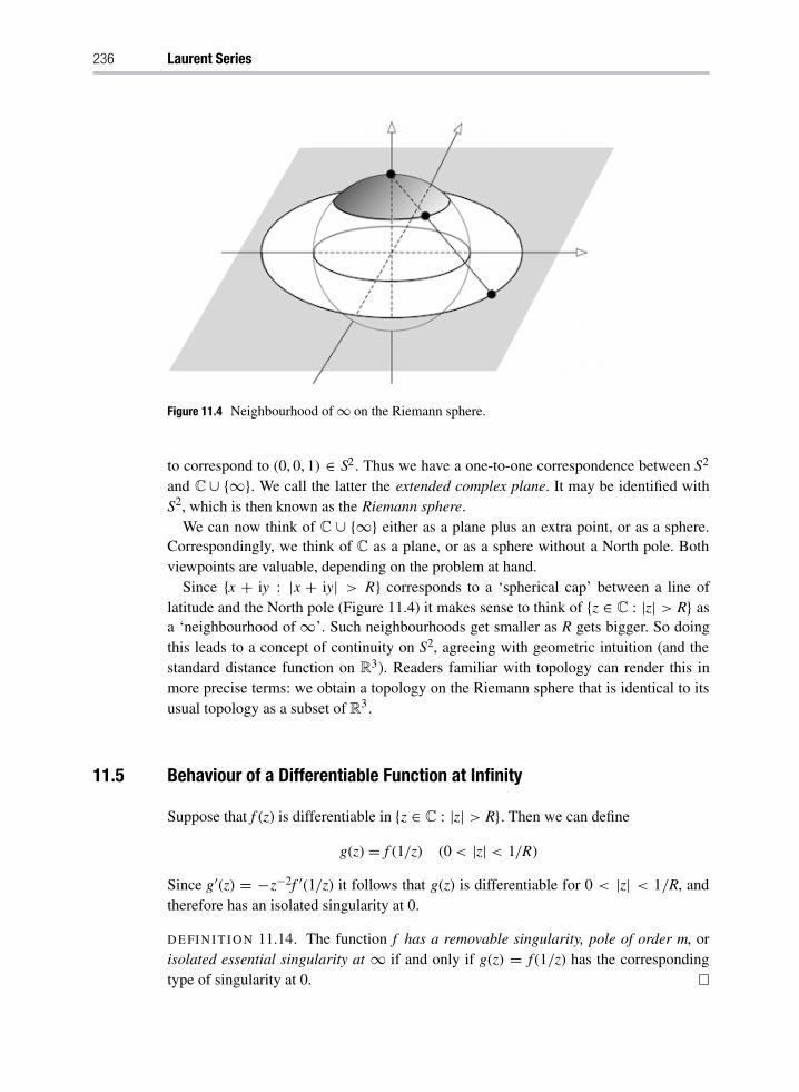
236 Laurent Series
Figure 11.4 Neighbourhood of∞ on the Riemann sphere.
to correspond to (0, 0, 1) ∈ S2 . Thus we have a one-to-one correspondence between S2
and C∪ {∞}. We call the latter the extended complex plane. It may be identified withS2, which is then known as the Riemann sphere.We can now think of C ∪ {∞} either as a plane plus an extra point, or as a sphere.
Correspondingly, we think of C as a plane, or as a sphere without a North pole. Bothviewpoints are valuable, depending on the problem at hand.Since {x + iy : |x + iy| > R} corresponds to a ‘spherical cap’ between a line of
latitude and the North pole (Figure 11.4) it makes sense to think of {z ∈ C : |z| > R} as
a ‘neighbourhood of∞’. Such neighbourhoods get smaller as R gets bigger. So doingthis leads to a concept of continuity on S2, agreeing with geometric intuition (and thestandard distance function on R3). Readers familiar with topology can render this inmore precise terms: we obtain a topology on the Riemann sphere that is identical to itsusual topology as a subset of R3 .
11.5 Behaviour of a Differentiable Function at Infinity
Suppose that f (z) is differentiable in {z ∈ C : |z| > R}. Then we can define
g(z) = f (1/z) (0< |z| < 1/R)
Since g²(z) = −z−2f ²(1/z) it follows that g(z) is differentiable for 0 < |z| < 1/R, andtherefore has an isolated singularity at 0.
DEFIN IT ION 11.14. The function f has a removable singularity, pole of order m, orisolated essential singularity at ∞ if and only if g(z) = f (1/z) has the correspondingtype of singularity at 0.

11.6 Meromorphic Functions 237
Example 11.15. f (z) = 1/z (|z| > 0). Then g(z) = z (|z| > 0), so f has a removable
singularity at∞.
Example 11.16. f (z) = z. Then g(z) = 1/z (|z| > 0), so f has a simple pole at∞.
Example 11.17. f (z) = ez. Then g(z) = e1/z (|z| > 0) and f has an isolated essentialsingularity at∞.
Example 11.18. f (z) = 1/(sin z) (z ±= nπ ,n ∈ Z). Then g(z) = 1/ sin(1/z). We cannotsay that f has an isolated essential singularity at∞, because f is not differentiable in{z ∈ C : |z| > R} for any R > 0. However, f certainly has some sort of singularity at∞.
In general, if f (z) has a sequence of isolated singularities zn such that zn → ∞, we saythat f has an essential (but not isolated) singularity at∞.
If f has a removable singularity at ∞ then g has a removable singularity at 0, somay be rendered differentiable in {z ∈ C : |z| < 1/R}. Thus we may say that f is
differentiable (or analytic) at∞, and define
f (∞) = g(0) = limz→0
g(z)
and nowf (∞) = lim
z→∞f (z)
For instance, if f (z) = 1/z then g(0) = 0 so f (∞) = 0.
Further, we say that f has a zero of order m at∞ if g has a zero of order m at 0. Thusif f (z) = 1/zm (|z| > 0,m ∈ Z,m > 0) then g(z) = zm and f has a zero of order m at∞.
In general, any statement about the behaviour of f at ∞ can be translated into oneabout g at 0 – and this is how to define or prove such a statement.
11.6 Meromorphic Functions
Poles are not, as singularities go, particularly nasty, and it is of interest to consider aclass of functions more general than differentiable ones.
DEFIN IT ION 11.19. If f is differentiable everywhere in a domain D except for pointsat which f has a pole, then f is meromorphic in D.
For instance, f (z) = 1/z is differentiable in C \ {0}, and has a pole at 0, so it ismeromorphic in C. Similarly, f (z) = 1/(sin z) is differentiable in C \ {nπ : n ∈ Z}, andhas poles at nπ, so it is meromorphic in C.We might go further, and consider functions meromorphic in the extended complex
plane – by which we mean that the only singularities of f , including∞, if necessary are

238 Laurent Series
poles. It is not necessary to introduce a special term for such functions, because theyturn out to have a simple description. Recall that a rational function is one of the form
f (z) = φ(z)/ψ (z)
where φ ,ψ are polynomial functions. Then we have:
PROPOSIT ION 11.20. A function is meromorphic in the extended complex plane if andonly if it is rational.
Proof. Clearly a rational function is meromorphic in C∪ {∞}.Suppose conversely that f is meromorphic in C∪ {∞}. Since f is differentiable at∞
or has a pole at∞, there exists R > 0 such that f is differentiable in
{z ∈ C : |z| > R}
So the poles, other than∞, occur inside the closed disc
{z ∈ C : |z| ≤ R}
Since poles are isolated singularities, each pole has a neighbourhood that contains noother poles. Indeed, if there were an infinite set S of poles inside |z| ≤ R, there wouldbe a limit point of S. This is not possible because the poles are isolated. This closeddisc contains only finitely many poles, say z1 , . . . , zk . Let the orders of these poles ben1, . . . ,nk. Define
g(z) = (z− z1)n1 · · · (z − zk)
nk f (z)
This is differentiable throughout C, hence analytic, so it has a Taylor series
g(z) =
∞±
n=0
anzn (z ∈ C)
Now the polynomial
ψ(z) = (z− z1)n1 · · · (z− zk )
nk
has a pole of order n1 + · · · + nk at∞, since
ψ
·1
z
¸=
·1
z− z1
¸n1
· · ··1
z− zk
¸nk
=1
zn1+···+nk+ · · ·
Since f has at worst a pole of order N at∞ for some N it follows that g(z) has a pole oforder
M = n1 + · · · + nk + N
at∞. Now
g(1/z) =
∞±
n=0
anz−n (|z| > 0)

11.7 Exercises 239
and since this has a pole of order M at 0 we must have an = 0 for n> M. Therefore
g(z) = a0 + · · · + aMzM
which is a polynomial, so f (z) = g(z)/ψ(z), which is rational.
A function meromorphic only in C need not be rational, as the example 1/(sin z)shows. This is not rational since it has infinitely many poles, but we have already seenthat it is meromorphic in C. So the behaviour at infinity is important.
11.7 Exercises
1. Find the Laurent expansions of the following functions of z around z = 0:
(i) (z− 3)−1
(ii) (z− a)−k (a ∈ C, k = 1, 2, 3, . . .)(iii) 1/(z(1− z))
(iv) 1/((z− a)(z− b)) (a,b,∈ C)(v) z3e1/z
(vi) exp(z+ 1/z)
(vii) cos(1/z)(viii) exp(z−5)In each case, specify the largest annulus in which the expansion is valid.
2. Find the Laurent expansions of the following functions on the stated annulus:(i) (z − 1)−2(z − 2)−1 on 0 < |z| < 1
(ii) (z − 1)−2(z − 2)−1 on 1 < |z| < 2
(iii) (z − 1)−2(z − 2)−1 on 2 < |z| < 3
(iv) exp(−z−2) on |z| > 0
(v) (1− z− z2)−1 in powers of z− 1 on 0 < |z− 1| < 1
(vi) ez/(1+ z2) on |z| > 1
3. Which of the following functions have a Laurent expansion around the given pointz0 (that is, in powers of z − z0)? (For multivalued functions, choose one particulardefinition on a domain that makes it single-valued.)(i)√z about z0 = 1
(ii)√z about z0 = 0
(iii) Log z about z0 = 0
(iv) Log z about z0 = 3
(v)»1+√z about z0 = 0
(vi) tan−1(1+ z) about z0 = 0
(vii) sin−1(z) about z0 = 0
(viii)
¼(π/2)− sin−1(z) about z0 = 1
(ix) z2cosec(1/z) about z0 = 0
(x)
¼(π/4)− sin−1(z) about z0 = 1/
√2

240 Laurent Series
4. Prove the validity of the Laurent expansion
1
(z− 1)(z− 2)=
∞±
n=0
2−(n+1)zn +
∞±
n=1
z−n
on a suitable annulus, and state which annulus.5. Find Laurent series for (z2 − 1)−1 and (z2 + 1)−1 in powers of z+ i and z− i, and
say in which annuli these are valid.6. Let a, b ∈ C. Show that
exp(az+ bz−1) =
∞±
−∞
anzn
where
an =1
2π
´ 2π
0
e(a+b) cos θ cos[(a− b) sin θ − nθ ]dθ
7. Let a ∈ C. Show that
sin(a(z + z−1)) =
∞±
−∞
anzn
where
an =1
2π
´ 2π
0sin(2a cos θ) cos nθ dθ
8. Find the poles of the functions:(i) 1/(z2 + 1)
(ii) 1/(z4 + 16)
(iii) 1/(z4 + 2z2 + 1)
(iv) 1/(z2 + z− 1)
9. Describe the type of singularity at 0 of each of the following functions:(i) sin(1/z) (z ±= 0)
(ii) z−3 sin2 z
(iii) z cot z (z ±= nπ ,n ∈ Z)
(iv) cosec2z− z−2 (z ±= nπ ,n ∈ Z)
(v) (cos z − 1)/z2
(vi) (sin z− z + z3/6)/z7
10. Let D be a disc centre z0 , let f be differentiable on D except at z0, and suppose that| f (z)| is bounded on D \ {z0}. Show that z0 is a removable singularity of f . (Hint:negative Laurent terms are 0 – why?)
11. Find all singularities of the following functions, and say which are poles:(i) (z + z−1)−1
(ii)cosπ z
1− 4z2
(iii) exp(z+ z−1)

11.7 Exercises 241
12. Construct a function defined on C∪ {∞} having only the following singularities:(i) A pole of order 2 at∞.
(ii) A simple pole at each of the points e2π ik/p , k = 0 , . . . ,p− 1, p an odd integer≥ 2.
(iii) A simple pole at z = 2 and a pole of order 5 at z =√2.
13. Let p(z), q(z) be polynomials of degrees m,n respectively. Describe the behaviour atinfinity of:(i) p(z)+ q(z)
(ii) p(z)q(z)
(iii) p(z)/q(z)
14. Find all singularities, and the behaviour at infinity, of the functions:(i) (z− z3)−1
(ii) z5/(2 − z2)2
(iii) (ez− 1)−1 − 1/z
(iv) cot 1/z(v) (cos z)z−2(vi) ((cos z)− 1)z−2
(vii) cot(1/z) − 1/z
(viii) sin(1/ cos(1/z))15. Let ± be a circle in the complex plane, or a straight line. Is its image on the Riemann
sphere also a circle?16. Find the poles and zeros of tan z. Show that tan z is meromorphic in C, but is not a
rational function.17. Show that (z + 1 + z−1)−1 has a removable singularity at z = 0. Find its Taylor
expansion, and the radius of convergence of this.18. Verify Picard’s Theorem directly for the functions:
(i) ez(ii) tan2 z(iii) z2
(iv) sin z(v) e1/z(vi) cos z(vii) tan z(viii) A function of your own choice.
19. Let f (z) have a pole of order n at z = a. Define the principal part φ(z) of f (z) to bethe sum of the negative-power terms in the Laurent expansion of f (z) in powers ofz− a. Prove that f (z)− φ(z) is differentiable at z = a.
20. Show that in a neighbourhood of a pole, a complex function is the sum of a rationalfunction and a differentiable one.
21. Suppose that f is differentiable on C except at poles, and that∞ is either a pole ora removable singularity of f . Show that:

242 Laurent Series
(i) f has only finitely many poles.(ii) f −
∑r pr is constant, where the poles of f are at points ar and the pr are the
corresponding principal parts of f (defined in Exercise 19).(iii) f is a rational function, and
∑r pr is its ‘partial fraction’ decomposition.
22. Let f : C → C be differentiable, with f (z) ±= 0 for all z ∈ C. Suppose thatlimz→∞ f (z) exists and is non-zero. Prove that f is constant.

12 Residues
Among the many applications of complex analysis are the explicit computation of def-inite integrals, the summation of series, and counting how many zeros a function has ina given region of C. Although such questions are not as important a part of pure math-
ematics as they once were, they are still very relevant to practical applications. Further,the power of the method and its wide applicability demonstrate the advantage of generalprinciples and deep theorems over manipulative ingenuity.The basic idea in all of these applications is to use Cauchy’s Theorem to exploit the
exceptional nature of the term b1/(z − z0) in the Laurent expansion of a differentiablefunction.
12.1 Cauchy’s Residue Theorem
The residue of f at z0 is determined by the special coefficient b1 just described:
DEFIN IT ION 12.1. If f has an isolated singularity at z0 and a Laurent expansion
f (z0 + h) =
∞±
n=0
anhn +
∞±
n=1
bnh−n (0< |h| < R)
then the residue of f at z0 isres ( f , z0) = b1
From Theorem 11.1 we immediately deduce that
res ( f , z0) =1
2π i
²
Cr
f (z)dz (12.1)
where Cr(t) = z0+eit (t ∈ [0, 2π ]) and 0< r < R. This shows the relevance of residuesto integration.
DEFIN IT ION 12.2. A closed path γ is a simple loop if every point z not on γ has
w(γ , z) = 0 or w(γ , z) = 1.
As usual, the set of points z ∈ C satisfying w(γ , z) ±= 0 (which in this case means
w(γ , z) = 1) are said to be inside γ .
In applications, simple loops will all be made up of straight line segments and parts ofcircles, as in Figure 12.1. All the simple loops encountered will be Jordan contours (that

244 Residues
Figure 12.1 Simple loops in C.
Figure 12.2 A simple loop in C that is not a Jordan contour.
is, they do not self-intersect), but that is not essential for the theory. (Figure 12.2 showsa simple loop according to our definition that is not a Jordan contour.) What matters isthat the points inside γ all have w(γ , z) = 1. (In particular, γ winds once anticlockwisearound such points.)In such cases, we have:
THEOREM 12.3 (Cauchy’s Residue Theorem). Let D be a domain containing a simpleloop γ and the points inside γ . If f is differentiable in D except for finitely many isolatedsingularities at z1, . . . , zn inside γ , then
²
γ
f (z)dz = 2π i
n±
r=1
res ( f , zr)
Proof. Since D is open we can find circles Sr(t) = zr + εreit (t ∈ [0, 2π]) round the zr
such that Sr and points inside it lie inside D, and such that Sr contains no singularity off other than zr , Figure 12.3. Then the collection of paths
−γ ,S1 , . . . ,Sn
satisfies the hypotheses of Theorem 8.9, because
w(−γ , z) = w(Sr , z) = 0 (z ±∈ D)
w(−γ , zr) = −w(γ , zr) = −1 since zr is inside γw(Sm, zr) = 0 if m ±= r, 1 if m = r

12.1 Cauchy’s Residue Theorem 245
Figure 12.3 Small circular contours around each isolated singularity.
Therefore
w(−γ , z)+ w(S1 , z)+ · · · + w(Sn, z) = 0
for all z ±∈ D.By the Generalised Cauchy Theorem,
²
−γ
f +
²
S1
f + · · · +²
Sn
f = 0
so that²
γ
f =
²
S1
f + · · · +²
Sn
f
= 2π i · res ( f , z1) + · · · + 2π i · res ( f , zn)
by (12.1).
Alternative Proof. Instead of the Generalised Cauchy Theorem we can use Laurentseries: the proof is instructive but less elegant. Around each zr there is a Laurentexpansion of f , which we split into three parts:
f (z) = Qr(z) +res ( f , zr)z− zr
+ Pr(z) (12.2)
where
Qr(z) =
∞±
n=2
bn(z− zr)−n
Pr(z) =
∞±
n=0
an(z− zr)n
Now Pr(z) is differentiable in a neighbourhood of zr, and Qr(z) + res ( f , zr)/(z− zr) isdifferentiable for z ±= zr since all but a finite number of the bn are zero. Therefore
h(z) = f (z)−
n±
r=1
Qr(z)−
n±
j=1
res ( f , zr)z− zr
(12.3)

246 Residues
is differentiable inD, except perhaps at z1, . . . , zn. But from (12.2) it is also differentiablein a neighbourhood of each zr. Hence h(z) is differentiable inD, so by Cauchy’s Theorem
²
γ
h(z)dz = 0 (12.4)
But Qr(z) = T²r(z) where
Tr(z) =
∞±
n=2
bn
−n+ 1(z− zr)
−n+1
so that ²
γ
Qr(z)dz = 0 (12.5)
as well. Integrating round γ and using (12.4) and (12.5), we get
0 =
²
γ
f (z)dz − 0−
n±
r=1
res ( f , zr)²
γ
(z − zr)−1
dz
=
²
γ
f (z)dz − 2π i
n±
r=1
res ( f , zr)
12.2 Calculating Residues
The Residue Theorem can be used to calculate integrals – and not just round simple
loops. For it to be of much use, we must find ways to calculate residues. The followingtwo lemmas are very useful in this respect.
LEMMA 12.4. (i) If z0 is a simple pole of f then
res ( f , z0) = limz→z0
(z− z0)f (z)
(ii) If f (z) = p(z)/q(z) where p(z0) ±= 0, q(z0) = 0, q²(z0) ±= 0, then
res ( f , z0) = p(z0)/q²(z0)
Proof. We have already done part (i) in the previous chapter as Proposition 11.10, butto recap: we have
f (z) =b1
z − z0+
∞±
n=0
an(z − z0)n
and so
(z− z0)f (z) = b1 +
∞±
n=0
an(z− z0)n+1
which tends to b1 as z→ z0 .
For (ii), note that
limz→z0
(z− z0)p(z)
q(z)= limz→z0
p(z)
³´q(z)− q(z0)
z− z0
µ
since q(z0) = 0, and this is equal to p(z0)/q²(z0).

12.2 Calculating Residues 247
For example, if
f (z) =cosπ z
z976
then
res ( f , 1) =cosπ
976 · 1975=
1
976
LEMMA 12.5. If z0 is a pole of f of order m then
res ( f , z0) = limz→z0
¶1
(m − 1)!
dm−1
dzm−1((z− z0)
mf (z))
·
Proof. We have
f (z) =bm
(z− z0)m+ · · · +
b1
z− z0+
∞±
n=0
an(z− z0)n
so that
(z− z0)mf (z) = bm + · · · + b1(z− z0)
m−1+
∞±
n=0
an(z− z0)m+n
Therefore
dm−1
dzm−1((z− z0)
mf (z)) = (m− 1)!b1 +
∞±
n=0
(m + n)!
(n+ 1)!an(z− z0)
n+1
Now take limits.
For example, consider
f (z) =
´z+ 1
z− 1
µ3
which has a triple pole at z0 = 1. Then
(z− 1)3f (z) = (z + 1)3
and so1
2!
d2
dz2((z− 1)3f (z)) =
6
2!(z+ 1)
which tends to 3 · 2 = 6 as z→ 1. So res ( f , 1) = 6.
On occasion another technique may be brought into play: working out the appropri-ate part of the Laurent series. (It is a waste to work out the whole thing, because thewhole point about residues is that we do not need the whole thing, but only b1 .) Forinstance:
f (z) =1
z2 sin z
= 1/
´z2´z −
z3
6+ · · ·
µµ
=1
z3
´1−
z6
6+ · · ·
µ−1

248 Residues
=1
z3
´1+
z6
6+ · · ·
µ
=1
z3+
1
6z+ · · ·
so that res ( f , 0) = 1/6.
12.3 Evaluation of Definite Integrals
We now consider a number of techniques for calculating various kinds of definiteintegral.
I:
± 2π
0
Q(cos t, sint)dt
Let C(t) = eit (t ∈ [0, 2π]) be the unit circle. If
z = C(t) = eit
then
cos t =1
2
´z+
1
z
µ
sin t =1
2i
´z−
1
z
µ
from which we get² 2π
0
Q(cos t, sin t)dt =²
C
Q
´1
2
´z+
1
z
µ,1
2i
´z−
1
z
µµdz
iz
= 2π i±
where ± is the sum of the residues of1
izQ
´1
2
´z+
1
z
µ,1
2i
´z−
1
z
µµ(12.6)
inside C.
For example, consider² 2π
0
(cos3 t + sin2 t)dt
Then (12.6) becomes
1
iz
¸1
8
´z +
1
z
µ3
−1
4
´z−
1
z
µ2¹=
1
8iz2 −
1
4iz+
3
8i+
1
2iz+
3
8iz2−
1
4iz3+
1
8iz4
which has a pole inside C with residue 1/2i. So the integral is 2π i/2i = π .

12.3 Evaluation of Definite Integrals 249
If Q is at all complicated, the computations can become very tedious. Sometimes
integrals of this kind can be found from the real and imaginary parts of an integral²
C
g(z)dz
with a suitable choice of g. For instance,²
C
ez
zdz = 2πi
since ez/z has residue 1 at z = 0. Therefore² 2π
0
ecos t+i sin t
eitdt = 2π i
so² 2π
0ecos t+i sin t
dt = 2π
and² 2π
0
ecos t [cos(sin t))+ i sin(sin t)]dt = 2π
Equating real and imaginary parts,² 2π
0
ecos t cos(sin t) = 2π
² 2π
0
ecos t sin(sin t) = 0
II:
±∞
−∞
f (x)dx
The real integral²∞
−∞
f (x)dx (12.7)
is defined to be
limx1→−∞, x2→∞
² x2
x1
f (x)dx (12.8)
provided the limit exists. The techniques we are about to discuss allow the calculationof
limR→∞
² R
−R
f (x)dx (12.9)
which is known as the Cauchy principal value of the integral, denoted by
P
²∞
−∞
f (x)dx

250 Residues
If (12.8) exists then so does (12.9) and the two are equal. But the Cauchy principal valuemay exist when (12.8) does not. For example
² R
−R
xdx = [x2/2]R−R = 0
so that
P
² R
−R
x dx = 0
But clearly (12.8) does not exist when f (x) = x.
It follows that when we use this technique below, we must take into account theconvergence of (12.8). This, in part, leads to condition (ii) of the following:
PROPOSIT ION 12.6. Suppose that:
(i) A function f is differentiable in the upper half-plane {z ∈ C : im z ≥ 0} except for afinite number of poles, none of which lies on the real axis.
(ii) If SR(t) = Reit (t ∈ [0, 2π ]) then there is a constant A such that for large R
|f (z)| ≤ A/R2
when z lies on SR.
Then ² ∞
−∞
f (x) dx = 2π i±
where ± is the sum of the residues of the poles of f in the upper half-plane.
Proof. Choose R large enough for (ii) to hold, and so that all the poles lie insideSR + [−R, R], Figure 12.4.By Cauchy’s Theorem,
² R
−R
f (x) dx+²
SR
f (z)dz = 2π i±
with ± as stated. Now let R→ ∞. Thenºººº²
SR
f (z)dz
ºººº ≤A
R2πR =
πA
R
Figure 12.4 Choice of R in proof of Proposition 12.6.

12.3 Evaluation of Definite Integrals 251
which tends to 0 as R→ ∞. Hence
limR→∞
² R
−R
f (x) dx = 2π i±
That is,
P
² ∞
−∞
f (x) dx = 2πi±
Now, (ii) tells us that |f (x)| ≤ A/x2 for large |x|, so it follows from real analysis that² ∞
−∞
f (x) dx
exists. It is therefore equal to its Cauchy principal value, hence to 2πi±.
REMARK 12.7. Condition (ii) is certainly satisfied if f (z) = p(z)/q(z) where p and q arepolynomials such that q has no real zeros and the degree of q is greater than or equal tothe degree of p plus 2.For example, consider
² ∞
−∞
dx
(x2 + a2)(x2 + b2)
where a, b > 0 are real, a ±= b. By Remark 12.7 this satisfies (ii), and (i) is obviouslytrue. The only poles of 1/((z2+ a2)(z2+ b2)) in the upper half-plane are simple poles atia, ib. The residue at ia is
limz→ia
z− ia
(z2 + a2)(z2 + b2)=
1
2ia(b2− a2)
and similarly that at ib is1
2ib(a2 − b2)
Therefore the value of the integral is
2πi
´1
2ia(b2 − a2)+
1
2ib(a2 − b2)
µ=
π
ab(a+ b)
REMARK 12.8. In the proof of Proposition 12.6 we do not require f (z) to be real for zon the real axis.
For instance, let
f (z) =eiz
(z2 + a2)(z2 + b2)
Then on SR we have |eiz| = |e−y+ix| = e−y ≤ 1 for y ≥ 0, so (ii) holds. As before, thereare simple poles at ia, ib, but now the residues are
e−a
2ia(b2 − a2)and
e−b
2ib(a2 − b2)

252 Residues
Hence²∞
−∞
eix
(x2 + a2)(x2 + b2)dx = π
´e−a
a(b2 − a2)+
e−b
b(a2 − b2)
µ
so, equating real and imaginary parts,²∞
−∞
cos x
(x2 + a2)(x2 + b2)dx =
π
b2 − a2
´e−a
a−
e−b
b
µ
² ∞
−∞
sin x
(x2 + a2)(x2 + b2)dx = 0
Of these, the second equality is actually obvious (why?), but the first is not.We can try to generalise this method in (at least) two ways: by getting a better estimate
for»SR
f or by allowing f to have poles on the real axis. The first is dealt with in (III),the second in (IV).
III:
±∞
−∞
f (x)eixdx
PROPOSIT ION 12.9. Suppose that:
(i) A function f is differentiable in a domain containing the upper half-plane {z ∈ C :
im z ≥ 0} except for a finite number of poles, none on the real axis.(ii) There is a constant A such that for large R
|f (z)| ≤ A/R for |z| = R
when z lies on SR. Then² ∞
−∞
f (x)eix dx = 2π i±
where± is the sum of the residues of the poles of f (z)eiz in the upper half-plane.
Proof. It is possible to use the same contour as in (II) and prove that
limR→∞
²
SR
f (z)eiz dz = 0
but this calculates only the Cauchy principal value. Moreover, the convergence problemin this case is much harder because all we know is that f behaves like 1/|x| for large |x|,which on its own does not imply the existence of
²∞
−∞
f (x)eixdx
More delicate arguments can overcome this obstacle, but it is easier to sidestep the wholequestion by using a different contour, as in Figure 12.5.

12.3 Evaluation of Definite Integrals 253
Figure 12.5 Contour for the proof of Proposition 12.9.
We prove that as X1,X2, Y→ ∞, each of²
²r
f (z)eiz dz
for r = 2, 3, 4 tends to zero. It then follows as before that
limX1,X2→∞
² X2
−X1
f (x)eixdx = 2πi±
as required.Now we carry out the necessary estimates,
ºººº²
²2
f (z)eiz dz
ºººº =ºººº² Y
0
f (X2 + it)eiX2−t idt
ºººº
≤
² Y
0
A
X2e−tdt
≤A
X2
for X2 large. Similarlyºººº²
²4
f (z)eizdz
ºººº ≤A
X1
Alsoºººº²
²3
f (z)eizdz
ºººº =ºººº−
² X2
−X1
f (t + iY)eit−Y
dt
ºººº
≤
ºººº² X2
−X1
A
Ye−Ydt
ºººº
= AY−1e−Y (X1 + X2)
For fixed X1 ,X2 this tends to 0 as Y → ∞. Now let X1 ,X2→ ∞.
As an example, take² ∞
−∞
x3eix
(x2 + a2)(x2 + b2)dx (a,b > 0, a ±= b)

254 Residues
which does not satisfy the conditions for (II), but does for (III). The integrand has simple
poles in the upper half-plane at ia and ib. Calculating the residues in the usual way,applying Proposition 12.9, and equating imaginary parts yields
²∞
−∞
x3 sin x
(x2 + a2)(x2 + b2)dx =
π
b2 − a2(b2e−b − a2e−a)
(Equating real parts proves that the corresponding cosine integral is zero, but again thisis obvious on other grounds.)
IV: Poles on the real axis.
If f (z) has poles on the real axis we make ‘indentations’ in the contour by drawing small
semicircles as in Figure 12.6. Suppose these semicircles have radii ε1 , ε2, . . .. Then weproceed as above, but letting ε1, ε2 , . . . tend to 0 at the same time as R,X1 ,X2,Y → 0.
There is a problem here similar to that in case (II): all we calculate is a Cauchyprincipal value
P
² b
a
f (x)dx = limε→0
¸² x0−ε
a
f (x)dx+
² b
x0+ε
f (x)dx
¹
for a pole at x0. This again may exist even if² b
a
f (x)dx = limε1→0
² x0−ε
a
f (x)dx+ limε2→0
² b
x0+ε
f (x)dx
does not. Thus² 1
−1
dx
x
does not exist, but
P
² 1
−1
dx
x= 0
Consequently there is a convergence problem, once the Cauchy principal value hasbeen obtained. Apart from this consideration, the hypotheses and conclusions of Propo-sitions 12.6 for case (II) and 12.9 for case (III) remain valid even when poles occuron the real axis, provided that ± is summed only over the non-real poles in the upperhalf-plane.
Figure 12.6 Types of contour used when there are poles on the real axis.

12.3 Evaluation of Definite Integrals 255
Figure 12.7 Contour used when there are poles on the real axis.
Rather than stating a cumbersome general theorem, we content ourselves with atypical example:
²∞
−∞
eix
xdx
There is a real pole at 0, so we take a contour as in Figure 12.7.As before, the integrals along ²2, ²3 , and ²4 tend to zero. Since there are no poles
inside the contour,
limX1,X2→∞
¶²−ε
−X1
eix
xdx+
² X2
ε
eix
xdx+
²
Cε
eiz
zdz
·= 0
But
eiz
z=
1
z+
∞±
n=1
inzn−1
n!=
1
z+ φ(z)
where φ is differentiable. Hence |φ(z)| ≤ M in a neighbourhood of 0, so
limε→0
²
Cε
eiz
zdz = lim
ε→0
²
Cε
´1
z+ φ(z)
µdz
= limε→0
´−
² π
0
1
εeitiεe
itdt
µ+ lim
ε→0
²
Cε
φ(z)dz
= iπ
using the Estimation Lemma. Therefore
P
²∞
−∞
eix
xdx = iπ
Equating real and imaginary parts,
P
²∞
−∞
cos x
xdx = 0
P
² ∞
−∞
sin x
xdx = π

256 Residues
The first integral exists only as a principal value, since cos(x)/x behaves like 1/x for
small |x|. But for the second we have
P
² ∞
−∞
sin x
xdx = lim
ε→0
´²−ε
−∞
sin x
xdx +
² ∞
ε
sin x
xdx
µ
= 2 limε→0
²∞
ε
sin x
xdx
This limit exists, hence by definition it equals
2
² ∞
0
sin x
xdx
because sin(x)/x→ 1 as x→ 0. Hence we can remove the P from the second expressionabove. Further, we have also proved that
² ∞
0
sin x
xdx =
π
2
V:
±∞
−∞
eax
φ(ex)dx
For integrals of this type we integrate around a contour like that in Figure 12.8.In this case, on ²3 , if we substitute z = −t + 2π i, then −X2 ≤ t ≤ X1, so that
²
²3
eaz
φ(ez)dz =
² X1
−X2
e−at+2π ia
φ(e−t+2π i)(−1)dt
= e2π ia²−X2
X1
e−at
φ(e−t )dt
Putting t = −x, this equals
−e2π ia² X2
−X1
eax
φ(ex)dx
If φ is such that²
²r
eaz
φ(ez)dz→ 0 as X1, X2 → ∞ (r = 2, 4)
then we obtain
(1− e2πai² ∞
−∞
eax
φ(ex)dx = 2π±
Figure 12.8 Contour for integrals of type (V).

12.3 Evaluation of Definite Integrals 257
where ± is the sum of the residues of eaz/φ(z) at poles between the lines im z = 0,
im z = 2π.
For example, consider² ∞
−∞
eax
e2x + 1dx (0 < a < 1)
The relevant singularities are at iπ/2, 3iπ/2, with corresponding residues
− 12eiπa/2 − 1
2e3iπa/2
Hence the value of the integral is
2πi
1− e2π ia(−1
2eiπa/2 − 1
2e3iπa/2)
Putting k = eiπa/2 this is easily seen to be equal toπ
2 sin(πa/2)
VI: Short cuts.
You should always be on the lookout for quick methods, other than those given above.We give two examples, each of independent interest.
Example 12.10. We use contour integration to prove that the integral of the ‘bell curve’or ‘gaussian’, which is of importance in probability theory, is
² ∞
−∞e−x
2
dx =√π
This result is usually obtained by squaring the integral, rewriting it as´² ∞
−∞e−x2
dx
µ ² ∞
−∞e−y2
dy
µ=² ∞
−∞
² ∞
−∞e−(x2+y2 )
dxdy
and then changing to polar coordinates. For a long time it was thought that no evaluationby contour integration existed, but several such proofs are now known. We give one ofthem, from Remmert [15]. Consider
f (z) = e−z2
1+ e−2az
with
a = (1+ i)
¼π
2
Then a2 = iπ , so
f (z) − f (z + a) = e−z2
(12.10)
The poles of f are simple and located at the points − 12a+ na with n ∈ Z.
Now integrate f over the rectangle with corners −r, s, s + i im(a),−r + i im(a) withr, s > 0. The only pole of f inside this rectangle is at a
2 , and its residue is

258 Residues
res( f ,a/2) =e− 14a
2
−2ae−a2=
−i2√π
This follows from Lemma 12.4, which states that
res½gh, x¾=
g(x)
h²(x)
if h has a simple zero at x and g(x) ±= 0.
Using the residue theorem and (12.10), it is easy to see that² ∞
−∞e−x
2dx = lim
r,s→∞
² s
−re−x
2dx = 2π i res( f , a/2)=
√π
since the integrals along the vertical sides of the rectangles converge to zero asr, s→ ∞.
Example 12.11. An integral of great importance in applied mathematics is² ∞
−∞eiλx
e−x2
dx (λ ∈ R)
The function e−z2 is differentiable throughout C. If γ is the rectangle with vertices at−R, R,R − iλ/2,−R − iλ/2, then
²
γ
e−z2
dz = 0
As R→ ∞, the integrals over the vertical edges of the rectangle tend to zero. The othertwo converge. Hence
² ∞
−∞e−x
2
dx =² ∞
−∞e−(x−iλ/2)
2
dx
=² ∞
−∞e−x
2eiλxeλ
2/4dx
Therefore ² ∞
−∞eiλxe−x
2dx = eλ
2/4
² ∞
−∞e−x2dx
The latter integral is a constant; it has just been evaluated in Example 12.10 and equals√π . So
² ∞
−∞eiλxe−x
2
dx = eλ2/4√π
(Although we can derive Example 12.10 from this by setting λ = 0, we need Exam-
ple 12.10 to get the result.)
12.4 Summation of Series
Residues can also be used to find explicit expressions for sums of suitable infiniteseries, based on the idea that the functions cotπ z and cosec π z have simple poles at

12.4 Summation of Series 259
z = n ∈ Z. If f is a function that is differentiable at all z = n ∈ Z then it is easy to checkthat
res ( f (z) cot πz, n) = f (n)
π
res ( f (z) cosecπz, n) =(−1)nf (n)
π
This suggests a method for summing certain series, as follows. Let CN be the squarewhose vertices are
(N + 12)(³1³ i)
parametrised, as usual, in the anticlockwise direction, Figure 12.9. We claim that cotπ zand cosecπ z are bounded on CN , where the bound is independent of N.To prove this, first note that on the two horizontal sides z = x + iy, where |y| ≥ 1
2 .
Now
| cotπ z| =ºººº
eiπ z+ e−iπz
eiπ z− e−iπz
ºººº
≤
ºººº
|eiπz| + |e−iπ z||eiπz| − |e−iπ z|
ºººº
=
ºººº
e−πy + eπy
e−πy − eπy
ºººº
= coth |πy|
≤ coth π/2
Also
|cosec πz| = ( 12|eiπz− e−iπz|)−1
≤ (12|e−π y − eπy|)−1
= (sinh |πy|)−1
≤ (sinhπ/2)−1
Figure 12.9 Square contour used to sum series.

260 Residues
On the other two sides of the square, z = ³(N + 12) + it, so
| cotπ z| = | tanh π t|
=
ºººº1− e−2π t
1+ e−2π t
ºººº≤ 1
and
|cosec πz| = | sinπ z|−1
= | cos(iπ t)|−1
= (cosh |πt|)−1
≤ 1
Hence there is a constantM such that | cotπ z| ≤ M and |cosecπ z| ≤ M for any z onCN .
Suppose now that for large enough |z| we have
|f (z)| ≤A
|z|2
Then we claim that± = 0
where ± is the sum of the residues of f (z) cot π z. By Cauchy’s Residue Theorem,²
CN
f (z) cot π zdz = 2πi±N
where ±N is the sum of the residues of f (z) cot πz inside CN . As N → 0, clearly ±N →
±, so it is sufficient to prove that the integral tends to 0. Butºººº²
CN
f (z) cot π zdzºººº ≤
A
N2M(8N + 4)
for large enough N by the Estimation Lemma. As N→ 0, this tends to 0 as claimed.
Usually, ± is an infinite series, and since it is zero we can sum certain related series.This is best illustrated by an example, and the obvious one to try is f (z) = 1/z2.
At an integer n ±= 0 the function z−2 cotπ z has a simple pole with residue 1/(n2π ),whereas at the origin it has a triple pole with residue −π/3. Hence
0 = ± = −π
3+
−1±
n=−∞
1
n2π+
∞±
n=1
1
n2π
= −π
3+
2
π
∞±
n=1
1
n2
Hence∞±
n=1
1
n2=π 2
6
which is a theorem originally proved by Euler, using a different (non-rigorous) method.

12.5 Counting Zeros 261
If we use cosec πz instead of cotπ z a similar result applies, allowing us to sum seriesof the form
∑(−1)nf (n). For instance, using f (z) = 1/z2 and arguing much as above,
we can prove that∞±
n=1
(−1)n+11
n2=π2
12
12.5 Counting Zeros
A rather different use for residues is to calculate the number of zeros of a function thatis differentiable inside a simple loop. We begin with:
THEOREM 12.12. Suppose that f is differentiable, apart from a finite set of poles, in adomain D containing a simple loop γ and all points inside γ . If f has no zeros or poleson γ then
1
2π i
²
γ
f ²(z)
f (z)dz = N − P
where N is the number of zeros of f inside γ and P is the number of poles of f inside γ ,each counted according to multiplicity.
Proof. By Cauchy’s Residue Theorem, the integral is the sum of the residues off ²(z)/f (z) at its poles inside γ . If z0 is neither a zero nor a pole of f , then f ²/f is
differentiable at z0 . We show that:
(i) If f has a zero of order k at z1 then f ²/f has a pole with residue k.(ii) If f has a pole of order m at z2 then f ²/f has a pole with residue −m.
To prove (i) note that in that case
f (z) = (z− z1)kφ(z)
where φ(z1) ±= 0 and φ is differentiable in a neighbourhood of z1. Therefore
f²(z) = k(z − z1)
k−1φ(z)+ (z− z1)
kφ²(z)
so
f ²(z)
f (z)=
k
z− z1+φ ²(z)
φ(z)
This has a simple pole at z1 with residue k, because φ ²/φ is differentiable at z1 . Thisproves (i).Similarly in case (ii)
f (z) =ψ(z)
(z − z2)m
where ψ(z2) ±= 0 and φ is differentiable in a neighbourhood of z2 . Therefore
f²(z) =
−mψ(z)
(z− z2)m+1
+ψ ²(z)
(z− z2)m

262 Residues
so
f ²(z)
f (z)=
−m
z − z2+ψ ²(z)
ψ(z)
which has a simple pole at z2 with residue −m.Now sum over all poles of f ²/f .
COROLLARY 12.13. Let γ be a simple loop in a domain D such that all points insideγ are in D. If f is differentiable in D and has no zeros on γ then the number of zeros off inside γ is
1
2πi
²
γ
f ²(z)
f (z)dz
From this we deduce another important theorem:
THEOREM 12.14 (Rouché’s Theorem). Suppose that f and g are differentiable in adomain D that contains a simple loop γ and all points inside γ . If
|f (z) − g(z)| < |f (z)| (12.11)
for all z = γ (t) (t ∈ [a,b]) then f and g have the same number of zeros inside γ .
Proof. Let F(z) = g(z)/f (z). By (12.11),
|1− F(γ (t))| < 1 (t ∈ [a, b]) (12.12)
Inside D,
F has a zero ⇐⇒ g has a zeroF has a pole ⇐⇒ f has a zero
Thus by Theorem 12.12 it is enough to prove that²
γ
F²(z)
F(z)dz = 0
To do so, let ²(t) = F(γ (t)). By (12.12),
|1− ²(t)| < 1 (t ∈ [a,b])
so ² lies inside the circle centre 1 radius 1, Figure 12.10. Now²
γ
F²(z)
F(z)dz =
² b
a
F²(γ (t))
F(γ (t))dt
=
² b
a
²(t)
²(t))dt
=
²
²
dz
z
= 2π iw(² , 0)= 0
from Figure 12.10.

12.6 Exercises 263
Figure 12.10 Path ² in proof of Rouché’s Theorem.
As an example of Rouché’s Theorem in action, we give a second proof of theFundamental Theorem of Algebra, Theorem 10.9. Let
g(z) = zm+ a1z
m−1+ · · · + am
f (z) = zm
Then
|f (z)− g(z)| = |a1zm−1 + · · · + am|
and for z ±= 0ºººº
1
zm
ºººº|f (z)− g(z)| =
ºººº
a1
z+ · · · +
am
zm
ºººº
The right-hand side tends to 0 as |z| → ∞, so there exists R > 0 such that if |z| > R
thenºººº
a1
z+ · · · + am
zm
ºººº< 1
and then|f (z)− g(z)| < |zm| = f (z)
Therefore by Rouché’s Theorem f and g have the same number of zeros inside {z ∈C : |z| < R}. Since f has m zeros (counting multiplicities) so does g. But g cannot
have more than m zeros, so every polynomial of degree m over C has exactly m zeros,
counting multiplicities. This is the Fundamental Theorem of Algebra.
12.6 Exercises
1. Find the residue of f at z0 in the following cases:(i) f (z) = z−3 sin z (z ±= 0), z0 = 0
(ii) f (z) = ezz−n−1 (z ±= 0), z0 = 0
(iii) f (z) = exp(1/z) (z ±= 0), z0 = 0

264 Residues
(iv) f (z) = z2(z2 + a2)−3 (z ±= ³ia), z0 = ia,−ia, where a ∈ R(v) f (z) = (1+ z2 + z4)−1 (z ±= exp (rπi/3), r = 1, 2, 4, 5), z0 = exp (π i/3)
2. Find the residue of the given function at each of its isolated singular points, includ-ing infinity (provided this is also isolated – that is, not the limit of a sequence offinite singularities).
(i) 1/(z3 − z5)
(ii) ez/(z2(z2 + 5))
(iii) cot3 z(iv) (sin z−1)−1
(v) (z cos z−2)−1
3. If f has a pole of order 2 at z0, show that the residue of f at z0 is h²(z0), whereh(z) = (z− z0)
2f (z).
4. Let γ (t) = eit, (t ∈ [0, 2π ]). Find, by residues, the value of²
γ
dz
z2 − 2az+ 1(a> 1)
Hence calculate² 2π
0
dt
a− cos t
What happens if a < −1? If −1 ≤ a≤ 1?
5. Verify the following:
(i)
² π
0
dt
1+ b cos2 t=
π√b+ 1
(b > −1)
(ii)
² ∞
0
dx
1+ x4=
π
2√2
(b > −1)
(iii)
² π
0
log x
1+ x2dx = 0
(iv)
² ∞
−∞
x sin πx
1− x2dx = π
(v)
² ∞
−∞
(log x)2
1+ x2dx = π 3
8
6. Show that² ∞
−∞
(10x)2
(x2 + 4)2(x2 + 9)2dx = π
7. Show that² ∞
0
cos 5xx4 + a4
dx = π
2a3e−5a/
√2 sin
´5a√2+ π
4
µ(a > 0)

12.6 Exercises 265
8. Evaluate:
(i)
² 2π
0
cos4 t + sin4 t dt
(ii)
² 2π
0sin
3t · cos t+ cos
3t · sin t dt
(iii)
² 2π
0
2 cos3 t + 3 cos2 t dt
9. If n ∈ Z,n > 0, prove:
(i)
² 2π
0
exp(cos t) cos(nt − sin t) dt = 2π/n!
(ii)
² 2π
0
exp(cos t) sin(nt− sin t) dt = 0
10. Evaluate, by integrating suitable functions round a semicircle:
(i)
² ∞
0
dx
1+ x2 + x4
(ii)
² ∞
0
cosmx
x2 + a2dx (a,m > 0)
11. Prove that²∞
0
x2
(x2 + a2)3dx =
π
16a3(a > 0)
12. By integrating round a rectangle whose vertices lie at R,R + i,−R + i,−R, andletting R→ ∞, show that
²∞
−∞
cosh(cx)
cosh(πx)dx = sec(c/2) (c ∈ [−π ,π ])
13. Prove that ²∞
0
ta−1(t + 1)−1 dt =π
sin πa(a ∈ [0, 1])
by making the substitution t = ex and integrating eaz(ez+1)−1 around the rectanglewith vertices ³R,³R + 2πi.
14. Inversion Formula for the Laplace Transform. Suppose that F is differentiable in Cexcept for a finite number of poles, of which z1, . . . , zn satisfy re z < a and none lieson the line re z = a. If there exist M > 0, b > 0, c > 0 such that |F(z)| < M/|z|c
for |z| < b, show that
f (t) = limR→∞
² a+iR
a−iReztF(z) dz = 2π i
n±
r=1
res(eztF(z), zr)
If F(z) = α(z2 + α2)−1 (α > 0) show that f (t) = sinαt.
15. Use real analysis to prove Jordan’s inequality:
sin t
t≥
2
π(t ∈ [0,π/2])

266 Residues
Hence show that if SR(t) = Reit (t ∈ [0,π ]) then
limR→∞
²
SR
eimz
zdz = 0 (m > 0)
By integrating eimz/z along the contours ²1 ,Cε ,²2, SR defined by:
²1(t) = t (t ∈ [−R,−ε])
Cε(t) = ei(π−t)
(t ∈ [0,π ])
²2(t) = t (t ∈ [ε,R])
prove Dirichlet’s Discontinuous Factor:
² ∞
0
sinmx
xdx =
⎧⎨
⎩
0 if m = 0
π/2 if m > 0
−π/2 if m < 0
16. Show that:
(i)z
ez− 1= 1−
z
2+
∞±
n=1
2z2
z2 + 4n2π 2
(ii) cosec z =1
z+
∞±
n=1
(−1)n2z
z2 − n2π2
(iii) cosec2 z =∞±
−∞
1
(z − nπ )2
17. Sum the following series, where a ±∈ Z:
(i)
∞±
−∞
(n+ a)−2
(ii)
∞±
0
(n2 + a2)−1
(iii)
∞±
0
(2n+ 1)−2
(iv)
∞±
0
(−1)n(2n+ 1)−3
18. By integrating
zeibz
(a2 − z2) sinπ z
round a suitable contour, show that
∞±
n=1
(−1)nn sinbn
a2 − n2=π
2
sinba
sinπa(|b| < π )

12.6 Exercises 267
19. By considering f (z) = 1/(z− ξ )+ 1/z, show that when ξ ±∈ Z,
π cotπξ =1
ξ+
∞±
n=1
2ξ
ξ 2 − n2
20. Using the result of Exercise 19, integrate π cotπx along a suitable contour to showthat
log sinπ z = logπ z+
∞±
n=1
log(1− z2/n
2)
where the log is chosen to make log 1 = 0 in each term. Taking exponentials, obtainthe infinite product expansion of the sine function (defined as the limit of suitablefinite partial products, by analogy with infinite sums):
sinπ z = π z
∞¿
n=1
(1− z2/n
2)
21. If |a| > e, use Rouché’s Theorem to prove that the equation
ez = azn
has n roots with |z| < 1.
22. Find the number of zeros of the following polynomials that lie inside the unit circle:(i) z9 − 2z6 + z2 − 8z− 2
(ii) 2z5 − z3 + 3z2 − z+ 8
(iii) z4 − 5z+ 1
23. How many zeros of z4+ 4z3 + 6z2 − 4z+ 3 lie inside the disc |z− 1| < 1?
24. Prove that however small ε > 0 is chosen, for all large enough n the function
1+ z−1 + (2!z2)−1 + (3!z3)−1 + · · · + (n!zn)−1
has all its zeros inside the disc |z| < ε.25. Let p(z) be a polynomial of degree n, and suppose that p(z1) = p(z2) = 0 with
z1 ±= z2 . Show that there exists a zero of p²(z) within the circle centre 12(z1+ z2) and
radius 12|z1− z2| cot(π/n).
26. Residues in Reverse. Show that the residue of tanp−1 πz at z = 12is (−1)p/2π−1 ,
for integer p > 0. (Hint: integrate it round the rectangle with vertices at −iR, 1 −iR, 1 + iR, iR, then let R→ ∞ and estimate sizes.)
27. Show that
(i)
² ∞
0
log x
1+ x2dx = 0
(ii)
² ∞
0
log x
(1+ x2)2dx = −π
4

13 Conformal Transformations
In mathematics we often encounter functions that preserve some structure that is ofinterest. For example, in Euclidean geometry rigid motions preserve lengths, angles,and areas, while changes of scale preserve the shape (but not the size) of geometric
figures. Homomorphisms of groups preserve group multiplication. Arithmetic modulo
n preserves addition and multiplication. Topological transformations preserve connect-edness. Conversely, given an interesting class of functions, we can ask what structurethey preserve. This chapter deals with a property preserved by all differentiable (equiva-lently analytic) complex functions, namely: angles between curves. Functions with thisproperty are called ‘conformal’.
The conformal property can be used in two directions. By studying differentiablefunctions, we can prove theorems about curves; by studying curves, we can prove theo-rems about differentiable functions. The second technique is of great importance in theadvanced ‘geometric’ theory of differentiable functions, but only the first falls withinour present scope. The method has interesting applications to potential theory and fluiddynamics, and we outline the beginning of these. We also consider in moderate detailseveral special conformal functions; in particular ‘Möbius maps’, often called ‘Möbius
transformations’, which have the remarkable property of mapping circles to circles.
13.1 Measurement of Angles
Since we are studying preservation of angles, we must discuss these first, in a manner
that is appropriate for this chapter. The use of a real number to measure an angle is notalways entirely satisfactory, because the same angle corresponds to many different realnumbers. However, if real numbers θ and φ represent the same angle, then θ − φ is
an integer multiple of 2π, and conversely, so the ambiguity is not too great. For many
purposes it can be avoided by making some artificial convention, such as the requirement
that −π < arg(z) ≤ π. For other purposes it is more convenient to measure angles in anatural and unambiguous way, though one that is less familiar than the real numbers.
13.1.1 Real Numbers Modulo 2π
If x, y ∈ R we say that x and y are congruent modulo 2π , and write
x ≡ y (mod 2π )

13.1 Measurement of Angles 269
if there is an integer n such that x− y = 2nπ. Congruence modulo 2π is an equivalencerelation, so it partitions R into mutually disjoint equivalence classes. We denote the setof all such equivalence classes by
R/2π
For each x ∈ R let p(x) be the equivalence class (or congruence class) to which x
belongs. This defines a function
p : R→ R/2π
and
p(x) = {x + 2nπ : n ∈ Z}
Given an angle measured by a real number θ , the same angle is measured by allθ + 2nπ (n ∈ Z), and by these real numbers only. Instead of picking one of them, wecan represent the angle by the whole collection, namely p(θ). In other words, the naturalmeasure of an angle is not a real number, but an element of R/2π .For instance, the real numbers
. . . ,−11π/3,−5π/3,π/3, 7π/3, 13π/3, . . .
all represent the same angle, and the set
{. . . ,−11π/3,−5π/3,π/3, 7π/3, 13π/3, . . .}
is the unique element of R/2π corresponding to this angle.
13.1.2 Geometry of R/2π
Geometrically, R/2π is a circle. To see this, define
q : R→ C q(x) = eix (x ∈ R)
The image of q is the unit circle in C, which we denote by
S = {z ∈ C : z = eix (x ∈ R)} = {z ∈ C : |z| = 1}
Since e2π i = 1, Proposition 5.3 shows that q(x) = q(y) if and only if x ≡ y (mod 2π ),so
q(x) = q(y) ⇐⇒ p(x) = p(y) (13.1)
Therefore we can define
j : R/2π → S
as follows: if r ∈ R/2π then r = p(x) for some x ∈ R, and we set
j(r) = q(x)
By (13.1) this is independent of the choice of x ∈ R, and j is a bijection. Thus theelements of R/2π are in natural one-to-one correspondence with the points of a circle.

270 Conformal Transformations
This bijection preserves continuity in a natural manner. If X ⊆ C we say that a func-tion f : X → R/2π is continuous if and only if the composite function j ◦ f : X → S
is continuous in the usual sense, considering S as a subset of C. This accords with theintuitive idea of geometric continuity if we think of R/2π as a circle. (In topologicalterms, we use j to transfer the usual topology of S to R/2π, defining U ⊆ R/2π to beopen if and only if j(U) is open in S. Continuity of maps f : X→ R/2π in this topologyis equivalent to what we have just defined.)
13.1.3 Operations on Angles
We can define addition and subtraction of elements of R/2π , corresponding to geo-metric addition and subtraction of angles. Let r, s ∈ R/2π. Pick x, y ∈ R such thatp(x) = r, p(y) = s, and define
r + s = p(x+ y)
r − s = p(x− y)
As usual we can verify that these definitions do not depend on the choice of x and y,
using (12.1).We can restate the above in group-theoretic terms. The set G = {2nπ : n ∈ Z} is
a subgroup of the additive group of real numbers, hence a normal subgroup since thelatter is abelian. The quotient group R/G is what we have called R/2π . As an analogy,consider the definition of the integers Zn modulo n as the quotient group Z/H where
H = {kn : k ∈ Z}.In Zn we can also define multiplication. You should verify that this does not work for
R/2π. It fails because 2π is not an integer. However, we can sensibly multiply an anglein R/2π by an integer, since this reduces to repeated additions or subtractions.
13.1.4 The Argument Modulo 2π
For z ∈ C \ {0} we can now define a ‘mod 2π’ version of arg z, namely
arc z = p(arg z) ∈ R/2π
The notation is deliberately chosen to resemble ‘arg’, and also reminds us that anglesare involved. The advantages of ‘arc’ over ‘arg’ are twofold. First, there is no ambiguity.
Second, and more important, the function
arc : C \ {0} → R/2π
is continuous. This is false for arg, for as z moves across the negative real axis, arg zjumps from near π to near −π, because of the convention that −π < arg z ≤ π . Incontrast, since p(−π ) = p(π ), this defect is not shared by arc. In fact, if z = reiθ , r > 0,
then j(arc(z)) = eiθ . Using this, or directly, it is not hard to verify that
arc(z1z2) = arc z1 + arc z2 (13.2)
for all z1, z2 ∈ C\{0}. Again if we use arg this is true only up to integer multiples of 2π .

13.2 Conformal Transformations 271
Thus we have two distinct ways to represent an angle: as a uniquely defined ele-ment of R/2π (an equivalence class of reals modulo 2π), or as a real number chosenfrom this class, unique only up to integer multiples of 2π . Both are useful, and thereare advantages in passing between them at will. We do this in the proof of our nextresult.
LEMMA 13.1. If γ : [a,b] → C is a path and γ ±(t0) exists and is non-zero for somet0 ∈ [a, b], then γ has a tangent at z0 = γ (t0) making an angle arc γ ±(t0) with the realaxis.
Proof. Let γ (t) = x(t)+iy(t). Then the required angle θ belongs to the congruence classmodulo 2π of
tan−1(y±(t0)/x±(t0)) = arg(x±(t0) + iy±(t0)) = arg γ ±(t0)
Taking congruence classes, we get
θ = arc γ ±(t0)
In future we will be less explicit about passing between R andR/2π .
DEFIN IT ION 13.2. If γ1 and γ2 are two paths meeting at z0 = γ1(t1) = γ2(t2) havingderivatives γ ±1(t1), γ
±2(t2) ²= 0, then the angle between γ1 and γ2 at z0 is
θ = arc γ±1(t1)− arc γ
±2(t2) ∈ R/2π
as in Figure 13.1.
Figure 13.1 Angle between two intersecting curves.
13.2 Conformal Transformations
In this section we consider functions f : D → C, where D is a domain. It is conve-nient to distinguish the two copies of C by using (x, y) as coordinates in D and (u, v) ascoordinates in the image C. As usual we let z = x + iy, and we set w = u + iv. (Theclassical notation for complex functions was w = f (z) before set theory came along.) Iff is differentiable on D we have
f (x+ iy) = u(x, y)+ iv(x, y)

272 Conformal Transformations
where u and v are real-valued functions of two real variables x, y. Hence f defines afunction from the subset D of the (x, y)-plane to the (u, v)-plane. A smooth path γ in D,with
γ (t) = x(t) + iy(t) (t ∈ [a,b])
is mapped by f to a path
fγ (t) = f (γ (t)) = u(x(t), y(t)) + iv(x(t), y(t)) (t ∈ [a,b])
in the (u, v)-plane.REMARK 13.3. Until now we have written composition as f ◦ γ , but from now on weomit the circle in formulas when there is no confusion with the product. This avoidsundue proliferation of circles.Suppose that z0 = γ (t0) and γ ±(t0) ²= 0 for some t0 ∈ [a,b]. By the chain rule,
( f γ )±(t0) = f ±(γ (t0))γ±(t0) = f ±(z0)γ
±(t0)
Therefore
arc (( fγ )±(t0)) = arc ( f ±(z0)γ ±(t0))= arc f ±(z0) + arc γ
±(t0) (13.3)
by (13.2).Suppose that γ1 and γ2 are two paths through z0, say z0 = γ1(t1) = γ2(t2). Then (13.3)
implies that fγ1 and fγ2 meet at the same angle as γ1 and γ2 . Geometrically this is clearsince both tangents are turned through the same angle arc f ±(z0). Alternatively, compute:
arc (( fγ1)±(t1))− arc (( fγ2)±(t2)) = arc f ±(z0) + arc γ ±1(t1) − arc f ±(z0)− arc γ ±2(t2)= arc γ ±1(t1)− arc γ
±2(t2)
DEFIN IT ION 13.4. A function f : D → C that preserves angles between paths at apoint z0 is conformal at z0.If f is conformal at all z0 ∈ D we say it is conformal.
The terms conformal function, conformal map, conformal mapping, and conformal
transformation all mean the same thing. The fourth is traditional, the third is going outof fashion, the second is convenient, and the first agrees with much current terminology.One advantage of the fourth is that it focuses attention on how paths and other geometricfigures transform under f .Observe that we have proved:
THEOREM 13.5. Let f : D → C be differentiable. The f is conformal at all z0 ∈ D
such that f ±(z0) ²= 0.
If f ±(z0) = 0 then f may not be conformal at z0 . For example, if f (z) = z2 then thepositive half of the real axis and the ‘positive’ half of the imaginary axis ({iy : y >0}) meet at right angles. They transform into the positive half of the real axis and thenegative half of the real axis, with an angle of π .
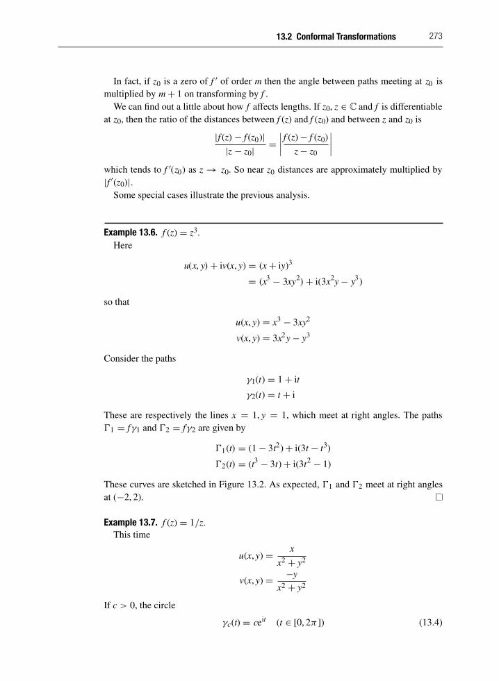
13.2 Conformal Transformations 273
In fact, if z0 is a zero of f ± of order m then the angle between paths meeting at z0 is
multiplied by m+ 1 on transforming by f .
We can find out a little about how f affects lengths. If z0, z ∈ C and f is differentiableat z0, then the ratio of the distances between f (z) and f (z0) and between z and z0 is
|f (z) − f (z0)|
|z − z0|=
±±±±
f (z)− f (z0)
z− z0
±±±±
which tends to f ±(z0) as z → z0. So near z0 distances are approximately multiplied by|f ±(z0)|.
Some special cases illustrate the previous analysis.
Example 13.6. f (z) = z3.
Here
u(x, y) + iv(x, y) = (x+ iy)3
= (x3− 3xy
2) + i(3x
2y− y
3)
so that
u(x, y) = x3 − 3xy2
v(x, y) = 3x2y− y3
Consider the paths
γ1(t) = 1+ it
γ2(t) = t + i
These are respectively the lines x = 1, y = 1, which meet at right angles. The paths±1 = fγ1 and ±2 = fγ2 are given by
±1(t) = (1− 3t2)+ i(3t − t3)
±2(t) = (t3− 3t)+ i(3t
2− 1)
These curves are sketched in Figure 13.2. As expected, ±1 and ±2 meet at right anglesat (−2, 2).
Example 13.7. f (z) = 1/z.
This time
u(x, y) =x
x2 + y2
v(x, y) =−y
x2 + y2
If c > 0, the circle
γc(t) = ceit (t ∈ [0, 2π ]) (13.4)

274 Conformal Transformations
Figure 13.2 Transformed paths for Example 13.6 also meet at right angles.
Figure 13.3 Images of circles centred at the origin for Example 13.7.
transforms into
±c(t) = c−1e−it (t ∈ [0, 2π ]) (13.5)
Hence the system of concentric circles (13.4), as c varies, maps into the system of con-centric circles (13.5), Figure 13.3. Further, the lines y = kx (k ∈ R) through the originare given by
δk(t) = t + kit
and transform to
²k(t) = (t + kit)−1 =1
1+ k2
1
t−
ik
1+ k2
1
t
which also represents lines through the origin. Now γc and δk all meet at right angles,and so do their transforms ±c and ²k, Figure 13.4.
Example 13.8. f (z) = sin z.
Here
u(x, y) = sin x cosh y
v(x, y) = cos x sinhy

13.2 Conformal Transformations 275
Figure 13.4 Paths for Example 13.7 and their transforms all meet at right angles.
Figure 13.5 Example 13.8: Cartesian coordinate grid transforms into a system of confocalhyperbolas and ellipses. Again all curves meet at right angles.
The lines x = c (c ∈ R) transform into confocal hyperbolas
u2
sin2 c−
v2
cos2 c= 1
and the lines y = d (d ∈ R) transform into confocal ellipses
u2
cosh2 d+
v2
sinh2 d= 1
as in Figure 13.5. The two systems of straight lines form a grid in Cartesian coordinates,crossing at right angles. The hyperbolas and ellipses also meet at right angles, except atpoints where f ±(z) = 0, namely f (z) = ³1. These are the common foci of the ellipsesand hyperbolas.

276 Conformal Transformations
13.3 Critical Points
Theorem 13.5 proves that a differentiable complex function is conformal at any point z0such that f ±(z0) ²= 0. We now consider what happens when f ±(z0) = 0.
DEFIN IT ION 13.9. Let f be a differentiable complex function. A point z0 is a regularpoint if f ±(z0) ²= 0. It is a critical point or singular point if f ±(z0) = 0.
Even though a complex function f need not be conformal near a critical point, thelocal geometry still has considerable structure. To unravel what happens at a criticalpoint, consider the local Taylor expansion:
f (z0 + h) = f (z0)+ hf ±(z0)+ · · · + hnf (n)(z0)/n! + · · ·
This consists of two parts. The constant part is w0 = f (z0), which calculates where thepoint z0 in the z-plane is mapped in the w-plane. The variable part
f (z0 + h) − f (z0) = hf ±(z0)+ · · · + hnf (n)(z0)/n! + · · ·
specifies how the function behaves near w0 = f (z0). In particular, the behaviour iscontrolled by the first non-zero derivative f (n(z0). This motivates:
DEFIN IT ION 13.10. A differentiable function f : D → C is of order n at z0 ∈ D,
(where n ≥ 1) if f (n)(z0) ²= 0, and f (k)(z0) = 0 for 1 ≤ k < n.
A function of order 1 satisfies f ±(z0) ²= 0, and in general, the Taylor series at a fixedpoint z0 for a function of order n has the form
f (z0 + h) = f (z0) + hnf (n)(z0)/n! + · · · (13.6)
Examples 13.11.(i) f (z) = zn for integer n≥ 1 is of order n.(ii) sin z = z− z3/3! + · · · is of order 1.(iii) cos z− 1= z2/2! − z4/4! + · · · is of order 2.
Equation (13.6) indicates that the behaviour of a function near a critical point is givenby the order of the corresponding zero of the derivative. Indeed, a function of ordern ≥ 1 can be written as:
f (z0+ h) = f (z0)+ khn + higher order terms in h, where k = f (n)(z0)/n! ² = 0
This gives an approximation of practical value in applications:
f (z0 + h) − f (z0) ≈ khn for suitably small h (13.7)
The size of h required to give a decent approximation depends on the context. As z
moves from z0−h to z0+h, the difference f (z)− f (z0) in (13.7) changes approximately
from k(−h)n to khn. The behaviour depends on whether n is even or odd. For n odd,

13.3 Critical Points 277
it moves from −khn to khn, passing through zero, and for n even it travels from khn to
zero, then back again to khn .
A more precise sense of the behaviour can be obtained by writing h in polarcoordinates, h = reiθ . For suitably small h, (13.7) gives
f (z0 + reiθ )− f (z0) = krneinθ + · · · (k = |f (n)(z0)|/n!)
so
|f (z0 + reiθ )− f (z0)| ≈ krn
and
arc ( f (z0 + reiθ )− f (z0)) ≈ nθ + α where α = arc ( f (n)(z0))
For small values of h, f transforms a tiny portion of the z-plane near z0 to the w-planenear w0 = f (z0), scaling r to krn and rotating the original angle θ to nθ +α, Figure 13.6.Rotating the line from z0 to z0 + h in the z-plane through a further angle φ rotates the
corresponding line in the w-plane to n(θ + φ) + α , so the angle between the trans-formed lines in the w-plane is nφ. The sector of the circle radius r, angle φ in thez-plane is scaled to a sector in the w-plane, radius krn , with angle expanded to nφ ,
Figure 13.7.For n = 1 the point is regular, and f is conformal. For n > 1, the function f transforms
z0 to w0 = f (z0), and a point distance r from z0 is scaled approximately to krn from w0
in the w-plane, while the angle between two paths through z0 changes from φ in thez-plane to nφ in the w-plane.
z-plane
w-plane
for suitably
small h
f
scale
to kr n
rotate to
nθ+α
z0
z0 +h
w0
f(z0 +h)
θ
r
Figure 13.6 The tangent map translating, rotating and scaling from z0 to w0.
Figure 13.7 Transforming a sector of a circle centre z0, radius r.

278 Conformal Transformations
13.4 Möbius Maps
For fixed a, b, c, d ∈ C, the function
f (z) =az+ b
cz+ d(ad − bc ²= 0)
is called a Möbius map or bilinear map. (Again, ‘map’ can be replaced by ‘function’,‘mapping’, or ‘transformation’.) These maps have a number of important properties, andwe discuss some of them.
First, note that f is differentiable for z ²= −d/c, and
f ±(z) =ad − bc
(cz+ d)2²= 0
since ad − bc ²= 0, again provided z ²= −d/c. Hence f is conformal throughout thedomain C \ {−d/c} on which it is defined.Now suppose that
f (z) =Az + B
Cz +D(AD − BC ²= 0)
is a second Möbius map. Then the composite
gf (z) =(Aa + Bc)z+ (Ab+ Bd)
(Ca+Dc)z+ (Cb+Dd)
is another Möbius map, because
(Aa+ Bc)(Cb+Dd) − (Ab+ Bd)(Ca+Dc) = (AD− BC)(ad − bc) ²= 0
So composing two Möbius maps always gives a Möbius map.
13.4.1 Möbius Maps Preserve Circles
A remarkable, and useful, property of such maps is that they transform circles (orstraight lines) into circles (or straight lines). To save breath, let us agree that in thissection a ‘circle’ may be either a circle or a straight line. (We can think of a straightline as a circle of infinite radius, remembering that∞ is a fairly respectable concept incomplex analysis.)Suppose p, q ∈ C with p ²= q, and let k > 0. The equation
|z− p|
|z− q|= k (13.8)
is satisfied by those points whose distances from p and q are in the ratio k. It is wellknown in Euclidean geometry, and can easily be checked using coordinates, that if k ²= 1
such points lie on a circle, and if k = 1 they lie on a straight line.Here is a quick proof. By scaling and a rigid motion, we can choose coordinates in
the plane so that p = (0, 0) and q = (1, 0). If (x, y) is distance kd from p, and distance dfrom q, then
²x2 + y2 = k
²(x− 1)2 + y2

13.4 Möbius Maps 279
Hence
x2+ y
2= k
2(x
2+ y
2− 2x+ 1)
which implies
³x−
k2
k2 − 1
´2
+ y2+
k2
k2 − 1−
³k2
k2 − 1
´2
= 0
which is the equation of a circle.If we put
w = f (z) =az+ b
cz+ d(ad − bc ²= 0)
it is easy to verify that
z =−dw+ b
cw − a
Now (13.8) takes the form±±±±±
az+bcz+d
− p
az+bcz+d − q
±±±±± = k
which simplifies to|w − P|
|w −Q|= K (13.9)
where
P = (b+ pa)/(d+ pc)
Q = (b+ qa)/(d+ qc)
K = k|d + qc|/|d+ pc|
Hence (13.9) also represents a circle. This proves that the Möbius map f transforms
circles into circles.
13.4.2 Classification of Möbius Maps
The above calculation, while it verifies the assertion, is not as instructive as we might
hope, and the following approach has its advantages. We consider several special typesof Möbius map that have especially simple forms, which can easily be seen to trans-form circles into circles. Then we show that a general Möbius map can be obtained bycomposing these types.It is perhaps not so surprising that this approach works, in view of the composition
property of Möbius maps. The decomposition can be seen as analogous to the well-known fact that any rigid motion of the Euclidean plane can be obtained by composing
a translation, a rotation, and a reflection.We begin with the special types.

280 Conformal Transformations
Translation: w = z + k (k ∈ C). This corresponds geometrically to moving pointsre k to the right and im k upwards, and clearly preserves the shape of geometric
figures, in particular circles.Rotation:w = eiθ z (θ ∈ R). All points rotate round the origin through angle θ . Again
this preserves the shape of geometric figures.Magnification: w = hz (h > 0). This produces a change of scale. If h < 1 it shrinks
rather than magnifies, but such pedantry is irrelevant and we still use the term‘magnification’. It therefore maps geometric figures to similar geometric figures.
Inversion: w = 1/z. Devotees of ‘inversive geometry’, now largely out of fashion,will recognise the corresponding ‘geometric inversion’, which is well known topreserve circles. However, circles can map to straight lines, or straight lines tocircles. The rest of us can check this by a coordinate calculation similar to the oneabove.
We can now state:
THEOREM 13.12. Every Möbius map can be obtained by composing a translation, aninversion, a magnification, a rotation, and another translation.
Proof. Suppose that a,b, c,d ∈ C and ad − bc ²= 0, where c ²= 0. Define
t1(z) = z+ d/c (translation)
j(z) = 1/z (inversion)
m(z) =
±±±±
ad − bc
c2
±±±±z (magnification)
r(z) =(bc− ad)|c|2
|ad − bc|c2z (rotation)
t2(z) = z+ a/c (translation)
It is routine to verify that
(t2rmjt1)(z) =az+ b
cz+ d
If c = 0 define
t1(z) = z+ b/a (translation
m(z) =±±±
a
d
±±± z (magnification)
r(z) =a
d
±±±±
d
a
±±±±z (rotation)
noting that ad − bc ²= 0 implies ad ²= 0 since c = 0, hence a ²= 0, d ²= 0. Now
(rmt1)(z) =az+ b
cz+ d
COROLLARY 13.13. Every Möbius map transforms circles into circles.

13.5 Potential Theory 281
There are other functions f : C → C that preserve circularity, the most obvi-ous being complex conjugation (which is not differentiable). A theorem of ConstantinCarathéodory asserts that every such function is either a Möbius map, or a Möbius
map composed with conjugation. No differentiability assumptions are needed for thistheorem. We do not prove it here.
13.4.3 Extension of Möbius Maps to the Riemann Sphere
There is a natural way to extend Möbius maps to the Riemann sphere by examining theirbehaviour as z→ ∞.
PROPOSIT ION 13.14. Any Möbius map can be extended uniquely to the Riemannsphere so that it is differentiable at every point.
Proof. By continuity we can find this extension by letting z → ∞, but we must thenverify differentiability. If
f (z) =az+ b
cz + d(ad − bc ²= 0)
then letting z→ ∞ we must define
f (∞) =
µ a
cif c ²= 0
∞ if c = 0
Differentiability at∞ is an easy exercise.
When extended in this manner, f is a bijection from C ∪ {∞} to itself. If we identifyC∪{∞}with the Riemann sphere S2 , then circles inC remain circles on S2 , and straightlines in C also become circles on S2.It is instructive to work out the effect of the basic types of Möbius map on S2 . We
omit the details.
13.5 Potential Theory
We now turn – briefly – to classical applications of complex analysis. These were instru-mental in convincing mathematicians that the subject was worth taking seriously, beforethe basic concepts had been made rigorous. We discuss potential theory, a general areaof mathematical physics with applications to gravitation electrostatics, magnetism, andfluid flow.
13.5.1 Laplace’s Equation
The two-dimensional Laplace equation
∂2φ
∂x2+∂2φ
∂ y2= 0

282 Conformal Transformations
for a function φ(x, y) is important in potential theory, with applications in particularto fluid dynamics. It is closely connected with complex function theory, as we nowdemonstrate. Let f : D →C be differentiable, with z = x+ iy, and write
f (z) = u(x, y) + iv(x, y)
as usual. Then
f ±(z) =∂u
∂ x+ i
∂v
∂x=∂v
∂y− i
∂u
∂y
as in Section 4.2. By Theorem 10.3 f ±± exists throughout D. If we let f ±(z) = U+ iV then
the Cauchy–Riemann Equations of Theorem 4.12 state that
∂U
∂x=∂V
∂y
∂V
∂x= −∂U
∂y
Therefore
U =∂u
∂x=∂ v
∂ yV =
∂ v
∂ x= −
∂u
∂y
so we get∂2u
∂ x2=
∂
∂x
³∂u
∂x
´=∂U
∂x=∂V
∂ y= −
∂
∂y
³∂u
∂y
´= −
∂ 2φ
∂y2
Therefore u(x, y) satisfies the Laplace equation. Similarly, so does v(x, y).For instance, consider f (z) = zez . Then
u(x, y) = xex cos y− yex sin y
v(x, y) = yexcos y+ xe
xsin y
and it may be verified directly that these functions satisfy Laplace’s Equation.Solutions of Laplace’s equation are called harmonic or potential functions. Pairs of
functions u, v obtained from a differentiable function by the above method are calledharmonic conjugates.The lines u = constant, v = constant, are orthogonal (mutually perpendicular) in the
(u, v)-plane, so by conformality the curves
u(x, y) = constant
v(x, y) = constant
are orthogonal in the (x, y)-plane. In potential theory, if u is harmonic, the lines u(x, y) =constant are called equipotential lines, and the set of orthogonal curves v(x, y) = con-
stant are called streamlines. In the case when Laplace’s equation describes fluid flow,streamlines are the paths along which the fluid flows. If we are given u in a domain D
and wish to find the streamlines given by v, we can often use complex integration. For afixed point z0 ∈ D, and any z1 ∈ D, we have
f (z1) =
¶ z1
z0
f±(z)dz =
¶ z1
z0
³∂u
∂x− i
∂u
∂ y
´dz

13.5 Potential Theory 283
For example, if u(x, y) = x2 − y2 , which is harmonic, then picking z0 = 0 forconvenience we have
f (z1) =
¶ z1
0(2x+ 2iy)dz =
¶ z1
02zdz = z
21
Hence f (x + iy) = (x + iy)2 = (x2 − y2) + i(2xy). So the streamlines have equations2xy = constant, or equivalently
xy= constant
Often, as in this case, we can guesswhat f , hence v(x, y), ought to be – a process dignifiedby the term ‘inspection’.
13.5.2 Design of Aerofoils
Conformal maps and complex function theory played a part in the design of aircraftin the early days of aviation (and, in a more sophisticated way, still do, although most
modelling is now done using the numerical methods of computational fluid dynamics).
In particular, the transformation from the z-plane to thew-plane given by
w − 2
w + 2=
³z− 1
z+ 1
´2
maps a circle in the z-plane, passing through −1 and containing +1 in its interior, intoa ‘bent teardrop’ shape as in Figure 13.8 that resembles a cross-section of an aircraft’swing. This is known as a Joukowski aerofoil, defined by a Joukowski transformation,after Nikolai Zhukovsky, who discovered the transformation.
Figure 13.8 Left: Flow past circle (with appropriate circulation added). Right: Circle transformed
to Joukowski aerofoil, with transformed flow.
It is used as follows. It is quite easy to solve the Laplace equation and find streamlines
for the flow of a fluid round a circular disc. Now apply the Joukowski transformation:
the disc maps to an aerofoil, and the streamlines round the disc map to the streamlines
round the aerofoil. In order to make the flow behave in a sensible physical manner at thesharp edge of the aerofoil, the flow past the circle is modified by adding a ‘circulation’term that flows round the circle. From this we can calculate properties of the flow; inparticular, the amount of ‘lift’ imparted to the aircraft. More subtle transformations, suchas the Karmann–Trefftz transform

284 Conformal Transformations
w − n
w + n=³z− 1
z+ 1
´n
give more accurate information.
13.6 Exercises
1. Sketch the image of the set D = {z ∈ C : re z > 0, im z > 0, |z| < 1} underthe conformal map f (z) = 1/z. Draw the images of the lines in D parallel to thecoordinate axes.
2. Show that the map
f (z) =√1+ k2
bexp
·−i
·π2+ tan−1 k
¸z
¸
transforms the strip between the lines y = kx, y = kx+ b into that between x = 0
and x = 1.
3. Find a conformal map f of the annulus 2 < |z| < 5 on to the annulus 4 < |z| < 10,
such that f (−5) = 10. (These points lie on the boundary so f must also be definedthere.) Find another with f (5) = 4.
4. With a suitable choice of the square root, show that
f (z) =√z − p− i
√p
maps the exterior of the parabola y2 = 4px (p > 0) onto the right-hand half-planex > 0, Figure 13.9.
5. Find a conformal map that sends the interior of the right-hand branch of thehyperbola
x2 − y
2 = λ2
to the upper half-plane y > 0, Figure 13.10. (Hint: what is re z2?)6. Show that the semicircle |z| < 1, re z > 0 is mapped by
f (z) = z2 + z
Figure 13.9 Conformal map of interior of parabola to half-plane.

13.6 Exercises 285
Figure 13.10 Conformal map of interior of hyperbola to half-plane.
Figure 13.11 Conformal map for Exercise 6.
Figure 13.12 Region for Exercise 7.
to the region bounded by the parabola x = −y2 and the curve whose equation inpolar coordinates is
r = 2 cos(θ/3) (|θ | ≤ 3π/4)
See Figure 13.11.7. Show that for suitably defined square roots, when a,b, c > 0,
f (z) =
¹ √z2 + c2 +
√a2 + c2
√bz2 + c2 −
√z2 + c2
maps the plane with the segments between −a, and b, and −ic and ic removed, tothe upper half-plane. See Figure 13.12.

286 Conformal Transformations
–1 + i
–1 – i 1 – i
–1 1
1
1 + ii
–i
Figure 13.13 Left: Region for Exercise 8. Right: Exterior of unit circle.
Figure 13.14 Region for Exercise 9.
8. Show that for suitably defined square roots,
f (z) = 1º2+
√5
³²ºz4 + 4+ 2+
²ºz4 + 4−
√5
´
maps Figure 13.13 (left) to the exterior of the unit circle, Figure 13.13 (right).9. Find a conformal map from Figure 13.14 to the upper half-plane. (Hint: compare
Exercise 7.)10. Show that
f (z) =»cosπ z− coshπh
1+ cosπ z
maps Figure 13.15 to the upper half-plane.11. Find a conformal map from Figure 13.16 to the upper half-plane.12. Find the Möbius map that sends −1,∞, i respectively to:
(i) i, 1, 1 + i
(ii) ∞, i, 1(iii) 0,∞, 1
13. Find the general form of a Möbius map that:(i) Transforms the upper half-plane to itself.(ii) Transforms the upper half-plane to the lower half-plane.

13.6 Exercises 287
Figure 13.15 Region for Exercise 10.
Figure 13.16 Region for Exercise 11.
(iii) Transforms the upper half-plane to the right half-plane.(iv) Preserves the unit circle.(v) Preserves the coordinate axes.(vi) Transforms the upper half-plane to the interior of the unit circle.
14. Invariance of Cross Ratio. The cross ratio of four complex numbers z1, z2 , z3 , z4 is
(z1− z2)(z3 − z4)
(z1− z4)(z3 − z2)
Let µ(z) =az+ b
cz+ dbe a Möbius map with ad − bc ²= 0, and let wj = µ(zj) for
j = 1, 2, 3, 4. Prove that
(w1 − w2)(w3 − w4)
(w1 − w4)(w3 − w2)=
(z1 − z2)(z3 − z4)
(z1 − z4)(z3 − z2)
(Hint: first work out how w1 − w2 relates to z1 − z2 .)
15. Let f be a Möbius map. A fixed point of f is a point z such that f (z) = z.
Prove that f has at most two distinct fixed points, including∞.
If f has a unique fixed point (including∞) it is said to be parabolic. Prove it canthen be written in the form
1
f (z) − z0=
1
z − z0+ h (z0 ²= ∞)

288 Conformal Transformations
or
f (z) = z + h (a translation)
If f has two distinct fixed points z1 , z2 , show that it can be written in the formf (z) − z1
f (z) − z2= k
z − z1
z − z2(z1, z2 ²= ∞)
or
f (z)− z1 = k(z − z1) (z2 = ∞)
Such a map is said to be hyperbolic if k > 0, elliptic if k = eiα (α ²= 0), andloxodromic if k = aeiα , where a ²= 1 is real and α ²= 0.
16. With the definitions of Exercise 14, prove the following:(i) Any Möbius map (az+ b)/(cz+ d) is equal to one for which ad − bc = 1.
(ii) Having ensured this, if a + d is real then the map is elliptic if |a + d| < 2,
hyperbolic if |a+ d| > 2, and loxodromic if |a+ d| = 2.
(iii) If a+ d is not real, the transformation is loxodromic.
17. Show thatu(x, y) = x
3− 3xy
2
is harmonic. Find a harmonic function v : R2 → R such that
f (x + iy) = u(x, y)+ iv(x, y)
is a differentiable complex function. Prove that v is unique up to the addition of areal constant.
18. For f (z) = 1/z, write f (z) = u(x, y) + iv(x, y). Sketch the level curves u(x, y) =constant, v(x, y) = constant. If a level curve of u meets a level curve of v, what isthe angle between them? Is there an easy way to see this, and if so, what is it?
19. Find the most general cubic polynomial
u(x, y) = ax3 + bx2y+ cxy2 + dy3 (a, b, c,d ∈ R)
that is harmonic. Find a differentiable function with u as its real part.20. Verify that the Joukowski transformation does, as claims above, give rise to an
aerofoil shape. Look up pages 131–134 of Kyrala [12] and see how to compute
streamlines round it. A more modern book is Anderson [1]. The NASA applet atwww.grc.nasa.gov/WWW/K-12/airplane/map.html is also worth investigating.

14 Analytic Continuation
When Weierstrass started his programme to rigorise complex analysis he based it onpower series. Because these have well-behaved convergence properties, and can bedifferentiated or integrated term by term, they provide a tool of great technical value.However, this tool has limitations, which we illustrate in the final section of this chap-ter: many important functions cannot be represented by a single power series – mainly
because power series converge on discs.
This limitation can be overcome by the method of ‘analytic continuation’, which letsus extend the domain of a complex function, subject to suitable conditions. It turns outthat such an extension is not always unique, and the problem of describing the differentpossibilities and how they are related leads to a remarkable geometric concept, knownas a ‘Riemann surface’ after its inventor. In this chapter we discuss these topics andrelated ones. Here we use the term ‘analytic’ rather than ‘differentiable’, to emphasise
the power series viewpoint – but you should remember that in the complex case theseterms are synonymous.
14.1 The Limitations of Power Series
We illustrate the problem for the function
f (z) =1
1− z2
It would be possible to use a simpler example, such as 1/z, but it is more appropriateto work with something a little less special, where the general problem is more sharplydefined
This function is analytic in C \ {−1, 1}, and has simple poles at−1 and 1. Its powerseries expansion about z0 = 0 is
1+ z2+ z
4+ z
6+ · · · (14.1)
which converges for |z| < 1 but diverges for |z| > 1. Thus if we require functions to bedefined on domains, the series (14.1) at best represents f on an open disc
D1 = {z ∈ C : |z| < 1}
Thus (14.1) tells us about a small part of f (directly, at least, although it has usefulindirect implications, as we shall see).

290 Analytic Continuation
We can begin to get round this problem by choosing a different z0, for example z0 = i.
To find the Taylor series for f (z) around z0 = i it helps to rewrite f in the form
f (z) = 1
2
±1
1+ z+ 1
1− z
²
Let w = z− i, so that z = w + i. Then
f (z) =1
2
±1
1+ w + i+
1
1− w− i
²
= 1
2
³1
1+ i
±1+ w
1+ i
²−1+ 1
1− i
±1+ w
1− i
²−1´
=1
2(1+ i)
∞µ
n=0(−1)n
±w
1+ i
²n
+1
2(1 − i)
∞µ
n=0
±w
1− i
²n
=∞µ
n=0
1
2
¶1
1+ i
±−11+ i
²n
+1
1− i
±1
1− i
²n·(z − i)n (14.2)
The series (14.2) has radius of convergence√2, because that is the distance from z0 = i
to the nearest pole of f , so it converges on
D2 = {z ∈ C : |z− i| <√2}
Figure 14.1 shows that (14.2) converges for some values of z for which (14.1) converges,and conversely. Thus not only do (14.1) and (14.2) represent small parts of f (namely itsrestrictions to D1 ,D2) but they represent different parts.Similarly if we take z0 = 2 we obtain a third series
f (z) =∞µ
n=0
¸−1
2 (−1)n + 1
6(−13)
n¹(z − 2)
n(14.3)
convergent on the discD3 = {z ∈ C : |z− 2| < 1}
Figure 14.1 Discs of convergence of various local power series for f . Shading shows intersectionsof discs.

14.2 Comparing Power Series 291
which represent yet another part of f . And something of this kind happens for any choiceof z0: the Taylor series
f (z) =
∞µ
n=0
an(z− z0)n (14.4)
converges for
|z− z0| < K = min(|z0 − 1|, |z0 + 1|)
by Theorem 10.3. Thus no single choice of z0 gives a power series expansion of f (z)valid for all z ∈ C \ {−1, 1}, even though f is analytic on this domain. (You shouldcheck that Laurent series do not improve the situation.)This problem is more a limitation of a tool – power series – than a defect of ana-
lytic functions. It is no fault of f (z) that our clumsy attempt to represent it using powerseries has apparently failed. The fact that a power series converges on a disc, so often ahelp, becomes a hindrance when we look at functions defined on domains that are notdiscs.
We could give up at this stage and ignore power series, but that would hardly beenterprising: it is a cardinal principle in mathematics not to throw away a good ideajust because it does not work. If a single power series is no good, why not try a wholecollection of power series? This solves part of the problem. We can certainly find, foreach z0 ∈ C \ {−1, 1}, a power series expansion (14.4) around z0 that converges to f (z)for all z near z0 . Thus using several power series gives information about the whole of f .However, it also creates another, more serious, problem. In the discussion so far
we started with f and worked out the power series. Weierstrass needed to proceed inthe opposite direction: use power series to define f (z). In the example above we knowthat the series (14.1), (14.2), and (14.3) represent the same function f , because that ishow they are constructed. If we are given two power series expansions around differ-ent points, how can we tell whether they represent the same analytic function, withoutknowing a priori what that function is? This is the central problem with Weierstrass’s
approach.
14.2 Comparing Power Series
We wish to compare two power series
p(z) =
∞µ
n=0
pn(z − z0)n
q(z) =
∞µ
n=0
qn(z − z1)n
around z0 , z1 respectively, convergent on open discs P,Q. Everything is easy if P and Q
overlap (that is, P ∩ Q ±= ∅), as is the case for (14.1) and (14.2), or (14.2) and (14.3),see Figure 14.2. In this case we can prove:

292 Analytic Continuation
Figure 14.2 Overlapping discs of convergence.
Figure 14.3 With more singularities, chains of discs may have to be longer.
LEMMA 14.1. Let f ,g be analytic on a domain D. Suppose that P and Q are open setsand ∅ ± = P ∩ Q ⊆ D. Suppose that p(z) = q(z) for all z ∈ P ∩ Q, and f , g are analyticfunctions defined on D such that f (z) = p(z) for z ∈ P and g(z) = q(z) for z ∈ Q. Thenf (z) = g(z) for all z ∈ D.
Proof. For z in the non-empty set P ∩ Q,
f (z) = p(z) = q(z) = g(z)
Now Theorem 10.16 implies that f (z) = g(z) for all z ∈ D.
In this sense, p and q represent the same analytic function. Obviously the conversealso applies: if p and q represent the same analytic function on D then they must agreeon the overlap.The existence of a non-empty overlap allows direct comparison of the two power
series: all we have to do is look at their values. But what if the discs of convergence donot overlap, as for (14.1) and (14.3)? The answer is to construct a chain of overlappingdiscs from one to the other, on each of which the power series converges, and suchthat the power series agree on all overlaps. Thus D1 and D2 overlap, and (14.1) agreeswith (14.2) onD1∩D2; andD2 andD3 overlap, and (14.2) agrees with (14.3) on D2∩D3 .
It is fairly clear that for f (z) = 1/(1−z2) we can get from D1 to any point z0 ±= ²1 by achain of at most three discs (two unless z0 is real and |z0 > 1|). For a more complicated
function with more poles (or other singularities) we may need more discs in a chain,because the discs have to ‘push between’ the singularities, see Figure 14.3. In a sensethis is the reason for the limitation of power series: discs are too blunt an instrument topenetrate beyond the singularities into more distant territory.

14.3 Analytic Continuation 293
When we formalise these ideas, as in the next section, it becomes clear that the restric-tion to power series is inessential. This is often the way in mathematics: the solution to aspecial problem turns out to apply in a much more general setting. The special problemplays the useful role of a psychological springboard, hurling our thoughts into higherrealms.
14.3 Analytic Continuation
The simplest type of analytic continuation is direct analytic continuation, extending afunction from one domain to an overlapping domain. Repeating this process we getindirect analytic continuation. We consider these in turn.
14.3.1 Direct Analytic Continuation
DEFIN IT ION 14.2. If f1 is analytic on a domain D1 and f2 is analytic on a domain D2 ,
where D1 ∩ D2 ±= ∅ and f1(z) = f2(z) for all z ∈ D1 ∩ D2, then f2 is a direct analyticcontinuation of f1 to the domain D2 , see Figure 14.4.
Such an f2 must be unique by Lemma 14.1.As a simpler example than that in the previous section, take
f1(z) =
∞µ
n=0
zn (|z| < 1)
f2(z) = 1/(1− z) (z ∈ C \ {1})
Then f2 is a direct analytic continuation of f1. Whereas f1 is defined only in the interiorof the unit disc, f2 is defined on the whole of C except at 1.Before going on to the general case, a series of overlapping domains, it is worth
dealing with another phenomenon. Sometimes D1 may be such that f1 has no directcontinuation to any D2 not contained in D1 . In this case the boundary of D1 is calleda natural boundary for f1. Now the limitation does not stem from our choice of tools,but from intrinsic properties of f1: it so happens that D1 is the end of the line as far asanalytic continuation of f1 is concerned.The standard example of this phenomenon is
Figure 14.4 Direct analytic continuation.

294 Analytic Continuation
f (z) =
∞µ
n=0
zn! (14.5)
which converges (so is analytic) for |z| < 1. We prove:
PROPOSIT ION 14.3. The unit circle S = {z ∈ C : |z| = 1} is a natural boundary forthe function f defined by (14.5).
Proof. Let z0 = eip/q for p,q,∈ Z, q≥ 1. Then zn!0 = 1 for all n ≥ q. We show first thatas z→ z0 then f (z) → ∞. Let z = rz0 where 0 < r < 1. Then
f (z) =
∞µ
n=0
(rz0)n!
= (1+ rz0 + · · · + r(q−1)!z(q−1)!0 ) +
∞µ
n=q
rn!
= g(r)+ h(r), say.
Note that h(r) has the above form because zn!0 = 1 for all n ≥ q. For any fixed integerN ≥ 0,
q+Nµ
n=q
rn!→ N + 1 as r → 1
So for some ε > 0, if 1− ε < r < 1, thenq+Nµ
n=q
rn!≥
12N
Then
h(r) =
∞µ
n=q
rn!≥
q+Nµ
n=q
rn!≥
12N
so that h(r)→ ∞ as r → 1, and h(r)→ ∞ as z→ z0. On the other hand,
g(z) = 1+ z0 + · · · + +r(q−1)!z(q−1)!0 as z→ z0
Therefore
limz→z0
f (z) = ∞ (14.6)
Now, suppose that F is a direct analytic continuation of f to a domain D2 not containedin D1 . Then ∂D1 ∩ D2 is open in ∂D1 = S, so it contains some point z0 = eip/q for
p,q,∈ Z, q ≥ 1 since such points are clearly dense on the unit circle. There is a small
disc Dε round z0 such that Dε ⊆ D2 . Now for 1 > r > 1− ε we have rz0 ∈ Dε , so that
F(rz0) = f (rz0)
As r→ 1,
F(rz0)→ ∞
by (14.6). But F is analytic in D2 , so

14.3 Analytic Continuation 295
Figure 14.5 Sequence of points tending to z0 .
Figure 14.6 Sequence of overlapping domains.
F(rz0) → F(z0)
as r → 1, by continuity. This is a contradiction; therefore no direct analytic continuationof f to D2, not contained in D1, is possible.
Figure 14.5 illustrates the geometry of this proof. Informally, the point is that thesingularities eip/q are so close together that there is no room to squeeze a disc betweenthem, onto which f might be analytically continued.
14.3.2 Indirect Analytic Continuation
We now return to the question of performing a sequence of direct analytic continuations,one after the other.
DEFIN IT ION 14.4. Let D1, . . . ,Dn be domains such that
Dr ∩Dr+1 ±= ∅ (r = 1, . . . ,n− 1)
as in Figure 14.6. If ( fr) is a sequence of analytic functions defined on Dr such thatfr+1 is a direct analytic continuation of fr (r = 1, . . . ,n − 1), then fn is an analytic
continuation of f1 from D1 toDn .
An analytic continuation that is not direct is an indirect analytic continuation.
Unlike the direct case, we may obtain different results by using different sequences ofdomains, Figure 14.7. Indeed, we can even have a sequence of overlapping domains forwhich Dn = D1 , but fn ±= f1, so that on returning to our starting point we end up witha different function from the original one. We illustrate this possibility by an example
in the next section. But first, we apply the above ideas to define a broader concept of ananalytic function.

296 Analytic Continuation
Figure 14.7 Sequences of overlapping domains that may lead to different analytic continuations.
14.3.3 Complete Analytic Functions
If f is analytic in a domain D we call the pair ( f ,D) a function element. We define arelation∼ on the set of all function elements by
( f1 ,D1) ∼ ( f2,D2)
if f2 is an analytic continuation of f1 from D1 to D2. Since indirect continuations areallowed, it follows easily that ∼ is an equivalence relation. A complete analytic functionis an equivalence class under ∼ of function elements.
In other words, a complete analytic function in the new sense is an analytic function inthe old sense, together with all of its analytic continuations. It is clearly more convenientto have the analytic continuations ‘built in’ than to have to fit them together as theoccasion warrants.If there exist function elements ( f1,D1 and ( f2 ,D2) of the complete analytic function
F such that for some z ∈ D1 ∩ D2 we have f1(z) ±= f2(z), we say that F is multiform. Ifnot, then F is uniform. All the examples considered so far in this chapter are uniform,
but we give examples of multiform functions in the next section. A multiform F is aformal version of the classical idea of a ‘multivalued function’, with the advantage thatit is broken down into pieces on each of which it is a genuine single-valued function.The multiformity arises because of how these pieces fit together. A geometric approachto this leads to the concept of a Riemann surface, discussed informally in Section 14.5.
14.4 Multiform Functions
A simple instance of a multiform function is
f (z) =√z
If z = reiθ then we can choose for√z either
√reiθ/2 or
√reiθ/2+π

14.4 Multiform Functions 297
where√r is real and positive. With the old concept of an analytic function, we must
choose one of these arbitrarily, and then f (z) is analytic only if we make a cut in thecomplex plane. From the present viewpoint, we can do better. We spell the method outin considerable detail – just this once.We introduce four domains:
H1 = {z ∈ C : re z > 0}H2 = {z ∈ C : im z > 0}H3 = {z ∈ C : re z < 0}H4 = {z ∈ C : im z < 0}
which are the open half-planes to the right, top, left, and bottom of the complex plane.Let z = reiθ where r > 0, θ ∈ [−π ,π ]. Define
f1(z) =√reiθ/2 for z ∈ D1 = H1
f2(z) =√reiθ/2 for z ∈ D2 = H2
f3(z) =º √
reiθ/2√rei(θ/2+π)
for
for
z ∈ D3 = H3 , im z ≥ 0z ∈ D3 = H3 , im z < 0
f4(z) =√rei(θ/2+π) for z ∈ D4 = H4
f5(z) =√rei(θ/2+π) for z ∈ D5 = H1
f6(z) =√rei(θ/2+π) for z ∈ D6 = H2
f7(z) =º √
rei(θ/2+π)√reiθ/2
for
for
z ∈ D7 = H3 , im z ≥ 0z ∈ D7 = H3 , im z < 0
f8(z) =√reiθ/2 for z ∈ D8 = H4
Each of these eight functions is analytic in its domain of definition; this is why for f3and f7 we have to change our choice of √z as we cross the imaginary axis, becauseotherwise our choice −π < θ ≤ π would introduce a discontinuity. Further, fr+1 is adirect analytic continuation of fr (r = 1, . . . , 7) and f1 is a direct analytic continuationof f8. For each z ∈ C \ {0} the values fr(z), where defined, are one or other of the twopossible square roots. Further, for each r, the function fr(z) takes one of the two valuesand fr+4 takes the other value, interpreting r+ 4 modulo 8 (and replacing 0 by 8).Thus we have defined a multiform function, taking two values at each z ±= 0. Going
round the origin once, fromD1 to D2 to D3 to D4 toD5 = D1, we reach a different valueof f (z) from the original one. However, in this case, going round a second time returnsus to the original value. This last effect is a special feature of √z, as the next exampleshows.
14.4.1 The Logarithm as a Multiform Function
Example 14.5. An immensely important multiform function is
f (z) = log z
Its multiformity was Euler’s great discovery, arising from the Bernoulli–Leibnizcontroversy mentioned in Chapter 0. In terms of the present discussion, we introducedomains

298 Analytic Continuation
D4k+r = Hr (k ∈ Z, r = 1, 2, 3, 4)
with the Hr as above. To avoid the kind of two-piece definition that occurred for f3 and
f7 above, we proceed as follows. For z ∈ Dn and z = reiθ where
n− 2
2π < θ ≤
n
2π
we definefn(z) = log r+ iθ
Then fn is analytic on Dn. On D1 ,
f1(z) = Log z
the principal value of the logarithm. On D5,
f5(z) = Log z + 2πi
On D4k+1,
f4k+1(z) = Log z+ 2kπ i
It is not hard to check that fs+1 is a direct analytic continuation of fs from Ds+1 toDs for
all s ∈ Z. For each r = 1, 2, 3, 4 and k ∈ Z the values of f4k+r(z) (z ∈ Hr) give all theinfinitely many possible values
log |z| + (2kπ + arg z)i
of the logarithm.
14.4.2 Singularities
We can now give a general definition of a singularity. If no analytic continuation of f canbe defined at a point z0 then we say that z0 is a singularity of the corresponding com-
plete analytic function. We have met several kinds of singularity before: poles, isolatedessential singularities, natural boundaries. Removable singularities are not singularitiesat all according to the new definition, because ‘filling in’ the missing point is a form ofanalytic continuation.For
√z and log z we encounter a new kind of singularity, called a branch point.
Analytic continuation round such a point leads to a change in value. Notice that forf (z) = √z there is even a natural definition of f (z) at the branch point itself, namely 0,but f is not analytic there. This is not the case for the logarithm.
Multiform functions make an appearance in contour integration whenever differentchoices of path from z0 to z1 leads to different values of the integral
F(z1) =» z1
z0
f (z) dz
(as may occur, for instance, if f has a pole in the region between the two paths). Hencequite nice singularities of f , such as poles, give rise to much nastier singularities of F,

14.5 Riemann Surfaces 299
namely branch points. This can occur even when f is uniform: for instance, 1/z is uni-form but its integral log z is multiform, and the pole of f at 0 has become a branch pointof F.
14.5 Riemann Surfaces
Riemann was a great geometer, and he invented a geometric way to envisage multiform
functions, which is much more intuitive than an equivalence class of function elements.
His idea is to replace C by a more complicated ‘Riemann surface’. Roughly speaking,the idea is to ‘glue together’ the domains of function elements at overlaps where thefunctions agree. We sketch this idea in general later; our immediate aim is to describe afew key examples.
14.5.1 Riemann Surface for the Logarithm
In the case of the logarithm we can describe the construction informally in the followingterms, which should not be subjected to too deep scrutiny of a logic-chopping kind. We
are not attempting a rigorous definition at this point; the informal description, though itmay sound far-fetched, is in fact capable of being given a rigorous rendering, describedat the end of this section.Consider a collection of copies Ck of C, one for each k ∈ Z. Slit each Ck along the
negative real axis from 0 to −∞. For each k join the top left-hand quadrant of Ck to
the bottom left-hand quadrant of Ck+1 along the slit. The resulting surface, Figure 14.8,resembles a spiral staircase or a concertina, with the planes stacked on top of each otherin order relative to k, and with a continuous spiral path from any Ck to any other Cl
going up the ‘steps’ where the slits were joined. These planes Ck are the sheets of theRiemann surface, and it is convenient to imagine the whole collection to be stacked ontop of C as shown in Figure 14.8.We define the logarithm for points on the Riemann surface by
log |z| + (2kπ + arg z)i
Figure 14.8 Riemann surface for the logarithm.

300 Analytic Continuation
Figure 14.9 A chain of overlapping domains that closes up inC no longer closes up when it istransferred to the Riemann surface.
Figure 14.10 Riemann surface for the square root – schematic of how the two sheets join.
where z is the point of Ck lying directly above the point z ∈ C. This is a single-valuedfunction on the Riemann surface, and it is continuous in the sense that the values joinup correctly across the cuts. (In a similar sense we can even say it is differentiable: thederivatives also join up correctly across the cuts.)Now we describe how to relate analytic continuation in C to the corresponding opera-
tion on the Riemann surface. Corresponding to a closed chain of domains D1, . . . ,Dn =D1 ⊆ C, we have D³1, . . . ,D
³n on the Riemann surface. In C the values of the functions
f1 , . . . , fn agree on the relevant overlaps D1 ∩ D2 , . . . ,Dn−1 ∩ Dn, but because of themultiformity they do not agree on D1 and Dn.
In contrast, on the Riemann surface we find that if we make D³1 and D³2 overlap, thenD³2 and D³3 , and so on, then by the time we get to D³n it no longer coincides with D³1because we have moved one level up the Riemann surface, see Figure 14.9. Hence D³1and D³n no longer overlap, and the difference between f1 and fn is only to be expected.The multiform nature of analytic continuation is automatically taken care of by the mul-
tiplicity of the sheets of the Riemann surface and how they join together. Even the natureof the singularity at 0 is apparent from the geometry of the surface, because here all thelevels meet.
14.5.2 Riemann Surface for the Square Root
Similarly for √z we obtain the Riemann surface by taking two copies C1 and C2 of
C, slit from 0 to −∞. Then join the top left-hand quadrant of C1 to the bottom left-hand quadrant of C2 along the slit; and similarly join the top left-hand quadrant of C2
to the bottom left-hand quadrant of C1 . (To do this in three-dimensional space requiresallowing the surface to intersect itself, but there is no conceptual problem here, seeFigure 14.10.)Again the phenomena noted above are clear from the geometry of the Riemann
surface: the two values of f (z), the fact that going round the the branch point at theorigin once changes the value but going round twice does not.

14.5 Riemann Surfaces 301
Figure 14.11 Gluing successive domains to form the Riemann surface of the logarithm.
14.5.3 Constructing a General Riemann Surface by Gluing
Obviously we cannot rely on such ad hoc methods to construct the Riemann surfacein general. We can approach the general method through the same example of thelogarithm, but building up the surface in a different way. Consider the sequence ofhalf-planes Ds and functions fs used for analytic continuation above. Suppose we takehalf-planes D³s corresponding to theDs, but make them pairwise disjoint. (The Ds are notdisjoint; for instance D1 = D5 and so on.) Then we ‘glue’ theD³s together in the follow-ing way: Ds andDs+1 overlap on a quadrant in which fs = fs+1, so we glue together thecorresponding quadrants D³s andD³s+1where they overlap. ThenD³2 glues on top ofD³1 atthe top right-hand quadrant; D³3 glues on to the top left ofD³2; D
³4 glues on to the bottom
left of D³3; and D³5 glues on to the bottom right of D³4. at this point D³5 is lying directly
over D³1, but we do not glue them together since f1 and f5 are different, Figure 14.11.Continuing with D³6,D³7 , . . . (and in the downward direction D³0,D³−1,D³−2, . . .) we buildup the spiral staircase Riemann surface again.The general method for constructing a Riemann surface of a complete analytic func-
tion F follows the same lines. Recall that F is an equivalence class of pairs ( f ,D) wheref is analytic on a domain D and ( f1 ,D1) ∼ ( f2 ,D2) if f1 , f2 are equal on the non-emptyset D1 ∩ D2 . We take disjoint copies D³λ of all the domains Dλ occurring in the pairs( fλ,Dλ ) that belong to F. If Dλ ∩ Dµ ±= ∅ and fλ = fµ on it, we glue D³
λto D³µ at the
points corresponding to the overlap Dλ ∩Dµ.
We make this description more rigorous. First, the question of ‘disjoint copies’ D³λof
Dλ. One way to achieve this is to define
D³λ = Dλ × {λ}
Then if λ ±= µ it is clear that D³λ∩ D³µ = ∅, and there is a natural bijection
jλ : Dλ → D³λ
defined by
jλ(s) = (s,λ) (s ∈ Dλ)
Now for that ‘gluing’. This is accomplished by a simple trick, using yet another equiva-lence relation, but it requires a certain amount of sophistication to appreciate that it doeswhat is required.

302 Analytic Continuation
Let
(zλ,λ) ≈ (zµ,µ)
for zλ ∈ Dλ, zµ ∈ Dµ, if:
(i) zλ = zµ
(ii) fλ(zλ) = fµ(zµ)
Then the set of equivalence classes under ≈ of points in the union of all the D³λ is
defined to be the Riemann surface of F. The equivalence relation ≈ acts as the glue.This definition is quite elegant, but might not be immediately appealing.The advantage of the Riemann surface construction is that we can now think of a
multiform complex analytic function as a genuine function, defined not on C but on theappropriate Riemann surface, rather than as an equivalence class of function elements.
The Riemann surface gives a ‘global’ view of the function, instead of chopping it up into‘local’ pieces. The last few sections of this chapter revisit previously discussed material
to explore some of the insights that can be gained in this way.
14.6 Complex Powers
So far we have considered powers za of a complex number z only for rational a, wherezp/q is a qth root of zp . We now define it for arbitrary a ∈ C. We would like to do this sothat the laws za+b = zazb and (za)b = zab, (zw)a = zawa remain valid. It turns out thatwe can ‘almost’ do this: however, za is in general multiform, and the formulas hold onlyif we choose appropriate values. Even when a is rational this problem already arises.A natural approach is to write
z = reiθ = elogr+iθ (14.7)
where log r ∈ R, and let a = α + iβ . On the assumption that the above laws hold, weobtain:
za = (reiθ )a
= ea(log r+iθ )
= e(α+iβ)(log r+iθ)
= eα log r−βθ ei(β log r+αθ ) (14.8)
We therefore define za by (14.8). This makes sense for all z ±= 0, and for all a ∈ C. Itamounts to requiring that
za = ea log z (14.9)
which is an equally natural way to define za. It follows that in any domain for which wemay define a unique branch of log (such as the cut plane Cρ for any ρ) we may alsodefine za as a single-valued differentiable function.In general, however, since log is multiform, so is za. To see what the possibilities are,
choose a particular value θ0 for θ (the obvious choice is the principal value of arg z).Then the possible θ that make (14.7) hold are of the form

14.6 Complex Powers 303
θ = θ0 + 2nπ (n ∈ Z) (14.10)
Write
(za)n = e
a(log r+i(θ0+2nπ))
which is the ‘nth branch’ of za , obtained by substituting θ from (14.10) into (14.8). Thequestion is now: how does (za)n depend on n?From (14.8) we have
(za)n = (e−2nπβ e2nπ iα)(za)0 (14.11)
where (za)0 is the 0th branch. Using (14.11) we can answer the above question. Thereare three cases:
(a) If β ±= 0 then za has infinitely many values, one for each n, because
|(za)n/(za)0| = (e−2nπβ )n
which takes distinct values for distinct n. The Riemann surface for za in this casehas the same form as that for the logarithm: an infinite ‘spiral staircase’ on whosenth layer the function is given by the branch (za)n .
(b) If β ±= 0, so a = α ∈ R, and if further α is irrational, then za = zα is again infinitelymany-valued, with distinct branch values for distinct n. For if (zα)m = (zα)n then
e2mπ iα = e2nπ iα , so e2π i(m−n)α = 1. This implies that (m− n)α ∈ Z by Section 5.7,which implies that m = n since α is irrational. The Riemann surface for zα is thesame as for case (a), but unlike case (a), the moduli of distinct branches are equal.Only the arguments vary.
(c) If β ±= 0, so a = α ∈ R, and if further α is rational, then we can write α = p/q in
lowest terms, where p,q ∈ Z. Now zα = q√zp.
Following the discussion in (b), two branches give the same values if and only if
(m− n)p
q∈ Z
which happens if and only if q divides m − n, because p and q have no common factorgreater than 1.It follows that the value of (zα)n depends only on nmod (q). The branches
(zα)0 , (zα)1, . . . , (zα)q−1
are distinct, but the qth branch repeats:
(zα)q = (zα)0
and repetitions continue thereafter.The Riemann surface, of course, is a q-sheeted spiral, with its top sheet glued to its
bottom one, as in our discussion of z1/2 but with q sheets instead of 2. Figure 14.12illustrates the case q= 5.

304 Analytic Continuation
Figure 14.12 Section through the Riemann surface for zp/q when q= 5, showing how the layersglue together.
Figure 14.13 Conformal map of a half-plane to a wedge.
Figure 14.14 How the conformal map of a half-plane to a wedge transforms streamlines.
14.7 Conformal Maps Using Multiform Functions
Conformal mapping with multiform functions requires careful attention to how valuesare specified; again, the simplest way to keep track is to put everything on a Riemann
surface. Here we consider only one case, of practical importance: the map z → zα for
real α ≥ 0. We assume the domain is the cut plane Cπ , on which the map may be definedto be single-valued.The great virtue of this map is that it transforms a half-plane into a wedge, as in
Figure 14.13. The vertex angle of the wedge is απ, so we have to assume α < 2 toprevent the image overlapping itself. The map is conformal except at the origin.For example, uniform fluid flow, with streamlines re z = constant, transforms to the
flow round a corner of angle απ , as in Figure 14.14.If we take α = 1/2, the corner is right-angled. Then z = x+ iy and z1/2 = w = u+ iv.
The flow-lines are x = constant. Now z = w2 so x = u
2−v2, y = 2uv. The streamlines in
the w-plane are given by u2−v2 = constant; they are branches of rectangular hyperbolas.

14.8 Contour Integration of Multiform Functions 305
Figure 14.15 Transferring a contour to a Riemann surface.
In combination with other ‘standard’ conformal maps, zα provides a useful weaponfor the applied mathematician.
14.8 Contour Integration of Multiform Functions
It is conventional to interpret a contour integral¼γ f of a multiform f by choosing the
values of f (z) so that they vary continuously along the contour. (This still leaves anarbitrary initial choice to be made, which must also be specified.) A more civilisedapproach is to break the contour γ into a sum γ = γ1 + · · · + γn such that:
(i) Each γj lies inside a domain Dj on which f may be defined as a single-valuedfunction.
(ii) On each Dj we choose a branch of f that makes the values agree where γj and γj+1join.
In terms of Riemann surfaces, we can interpret this process as the definition of acontour integral when the contour lies on the Riemann surface. The way the contourwanders up and down the staircases on the surface automatically takes care of the choiceof values of the multiform function f (z), see Figure 14.15. In practice this is all more
straightforward than it may sound, and the computations are no harder than the uniformcase – provided you use your head.
Example 14.6. Let γ be the contour
γ (t) = (1+ t)eit (t ∈ [0, 6π ])
Find »
γ
z1/5
dz
Method 1 (stupid): Defining z1/5 on the contour by (γ (t))1/5 = (1 + t)1/5eit/5 makes itvary continuously with t. By Theorem 6.6

306 Analytic Continuation
Table 14.1 Choice of θ.
domain θ chosen in interval
D1 [−π/4, 5π/4]D2 [3π/4, 9π/4]D3 [7π/4, 13π/4]D4 [11π/4, 17π/4]D5 [15π/4, 21π/4]D6 [19π/4, 25π/4]
Figure 14.16 Six overlapping domains.
»
γ
f (z)dz =
» 6π
0
( f (γ (t))γ ³(t) dt
=
» 6π
0
(1+ t)1/5eit/5(ieit + iteit + eit) dt
which leads the hopeful calculator along some fascinating byways inhabited by integralssuch as
» 6π
0
t(1+ t)1/5 cos(6t/5)dt
A wise person knows when to cut their losses.Method 2 (sound but pedestrian): Cover the contour γ by domains in which z1/5 may
be given a unique value for each z, which is differentiable. For example, we can findsix domains D1 , . . . ,D6, one for each of the intervals AB, BC, CD, DE, EF, FG inFigure 14.16.To make the values match on overlaps we choose the definition of z1/5 as follows.
Write z = reiθ where the choice of θ is as in Table 14.1.On each domain choose the branch of z1/5 given by r1/5eiθ/5 with θ in the range stated
in the table. These choices make θ agree on overlaps.

14.8 Contour Integration of Multiform Functions 307
Break up the integral as»
γ
=
»
AB
+
»
BC
+
»
CD
+
»
DE
+
»
EF
+
»
FG
In each domain Dj the function z1/5 has an antiderivative 56 z6/5 where z6/5 is defined
using the corresponding branch z6/5 = r6/5e6iθ/5 . By Theorem 6.33, if PQ is any of thearcs AB, BC, and so on, then
»
PQ
z1/5dz = 56Q
6/5−
56P6/5
When we add the six expressions of this type, all terms but two cancel, so the integral is56G
6/5−
56A
6/5
Here A = γ (0) = 1, G = γ (6π) = (1 + 6π )e6iπ . Evaluate the 6/5th powers accordingto the above prescription:
A6/5 = (1 · ei0)6/5 = 1
G6/5= (1 + 6π )e
6π i)6/5= (1+ 6π)
6/5e36iπ/5
= −(1+ 6π )6/5eiπ/5
Therefore the integral is equal to
−56[(1 + 6π )
6/5eiπ/5 + 1]
Method 3 (slicker): In terms of the parameter t we can define the required branch of z1/5to vary continuously along the contour γ if we put
z1/5 = (γ (t))1/5 = (1+ t)1/5eit/5
There is a local antiderivative 56z6/5 , whose value varies continuously along the path γ
if we choose branches so that
(γ (t))6/5 = (1 + t)6/5e6it/5
Now pave γ by a finite number of domains, on each of which z1/5 may be renderedsingle-valued, choosing the branches to agree with those already chosen on the path. Asabove, the integral may be expanded as a sum of terms of the form
56[(1 + tj+1)
6/5e6it j+1/5 − (1+ tj)6/5e6it j/5]
where the tj subdivide the interval over which t runs. All but two terms cancel, leavingthe same answer as before.The advantage of this method is that by choosing branches in an obvious way for
γ (t) we may leave the prescription of the domains, and the branches on those domains,implicit.
Method 4 (smart): Let the Riemann surface do the work. The above analysis easilygeneralises to give a version of Theorem 6.33 for multiform functions, integrated along

308 Analytic Continuation
a contour in the Riemann surface. Given a global antiderivative F for f on the Riemannsurface, we have
»
γ
f = F(z1) − F(z0)
where z0 is the initial point, z1 the final point, and the branches are chosen with referenceto the end points of γ on the surface, as in Figure 14.15. This gives the result almostimmediately on noting that γ winds three times anticlockwise, so the 6/5th power winds3 · 6/5 = 18/5 times anticlockwise, giving for F(z1) the argument 2π · 18/5 − 36π/5,if we choose argument 0 for z0.
We leave it as an exercise to formulate and prove generalisations of Cauchy’s Theo-rem for contour integrals on the Riemann surface of a multiform function. For those whoprefer not to use the insight that Riemann surfaces provide, however, we recommendMethod 3 above as a relatively direct and simple technique.
Example 14.7. Example 14.6 is of course a bit artificial, and its main interest is ped-agogical. A more typical example of integrals likely to be encountered in practiceis » ∞
0
xa
1+ x2dx (a ∈ R, 0 < a < 1)
Note that the restrictions on a make this integral converge, so the question is sensible.We begin with the complex function
f (z) = za(1+ z2)−1
which is differentiable for all z ±= 0, i,−i, and is multiform for all a in the given range.Make a cut along the positive real axis and work in the cut plane C0 (in the notation
of Section 2.2). On this domain za may be rendered single-valued: set (reiθ )a = raeaiθ
where θ ∈ [0, 2π ]. Now integrate f (z) along the contour γ in Figure 14.17. This runsfrom the real point ρ to the real point R, then once anticlockwise round the circle ofradius R, then back to ρ, then once clockwise round the circle radius ρ.
Figure 14.17 Contour for Example 14.7.

14.8 Contour Integration of Multiform Functions 309
By Cauchy’s Residue Theorem, Theorem 12.3,»
γ
f (z)dz = 2πi (± residues inside γ )
We intend to let ρ → 0 and R→ ∞, so we may as well assume that ρ < 1 and R > 1.
Then the singularities inside γ are z = ²i. We calculate the residues at these points asfollows:
At z = i the residue is
α = limz→i
za/(z+ i) =1
2π ieiaπ/2
At z = −i the residue is
β = limz→−i
za/(z− i) =
1
2π ieia3π/2
Let the circle of radius R be γ1, and that of radius ρ be γ2. Then Cauchy’s ResidueTheorem implies that» R
ρ
xa
1+ x2dx+
»
γ1
za
1+ z2dz+
» ρ
R
(xe2π i)a
1+ x2dx+
»
−γ2
za
1+ z2dz = 2π i(α+β) (14.12)
Note that in the third integral we must choose the branch of za corresponding to argu-ment 2π, to retain continuity. Now let ρ → 0 and R → ∞. Easy estimates show thatthe second and fourth integrals tend to zero. The first tends to
»∞
0
xa
1+ x2dx
and the third to
−e2π ia
» ∞
0
xa
1+ x2dx
Therefore
(1− e2π ia
)
» ∞
0
xa
1+ x2dx = 2πi
±1
2π ieiaπ/2
−1
2π ieia3π/2
²
After some manipulation, this leads to»∞
0
xa
1+ x2dx =
π
2 cos(aπ/2)
Yes, but . . . did you spot the nifty footwork? The chosen contour does not actuallylie inside the domain C0 . Nonetheless, the result is correct. There are several ways tojustify the answer rigorously. They include:
(1) Replace γ by a contour that starts just above ρ , say at ρ + iε, runs horizontally tojust above R at R + iε, circles γ1 to just below R at R − iε, runs back to below

310 Analytic Continuation
Figure 14.18 Modified contour remains inside C0 .
Figure 14.19 Lifting γ to the Riemann surface.
ρ at ρ − iε, and the goes back round γ2 as in Figure 14.18. Now, as ρ → 0
and R → ∞, make the width 2ε of the channel tend to zero and use continuityarguments.
(2) The choice of C0 causes problems, so reject it. Work in two overlapping domains,
say C−π/4 and Cπ/4, and switch between them when defining the second, third, and
fourth integrals in (14.12).(3) Put it all on a Riemann surface. The contour γ then winds round the staircase and
up one step, then winds back down one step to get back to the start.
Everything generalises to such contours, because they are obviously boundaries ofrectangles in the Riemann surface, Figure 14.19. This argument is an example of the‘homology’ version of Cauchy’s Theorem, when generalised to Riemann surfaces. We
discuss homology in Chapter 16, but do not extend the ideas to Riemann surfaces sincethis would take us too far afield.These three approaches justify the computational method rigorously. Of course, when
performing the calculations, it is not necessary to trot out such a justification every time
– provided you understand how it would go. Everything works fine as long as you followthe golden rule: make the multiform function vary continuously as you walk round thecontour.

14.9 Exercises 311
14.9 Exercises
1. Define three power series by
a(z) = 1+ z+ z2 + z3+ · · · =∞µ
n=0
zn
b(z) = i− (z− i − 1)− i(z− i − 1)2+ (z− i− 1)
3+ · · · =
∞µ
n=0
in+1
(z− i− 1)n
c(z) = −1+ (z− 2) − (z− 2)2+ · · · =
∞µ
n=0
(−1)n+1
(z− 2)n
Find their discs of convergence and sketch them. Prove that a(z) = b(z) on theoverlap of their discs of convergence, and similarly that b(z) = c(z) on the overlapof their discs of convergence. Do the discs of convergence of a(z) and c(z) intersect?
2. Let f (z) =∑∞n=0 an(z − z1)
n and g(z) =∑∞n=0 bn(z − z2)
n be two power series,and assume that their discs of convergence have non-empty intersection. Prove thatg is a direct analytic continuation of f if and only if there exists z0 in both discs ofconvergence such that form = 0, 1, 2, 3, . . . the equations
mµ
n=0
n(n− 1) · · · (n−m)[an(z0 − z1)n−m − bn(z0 − z2)
n−m] = 0
hold.
3. A certain function has singularities at precisely the points z such that re z and im z
are integers. You are given its Taylor expansion around the point 12+ 1
2i. What is
the smallest number of stages needed to find an indirect analytic continuation, bypower series, to a domain that contains 7
2 +52 i?
4. Show that the functions defined by(i) f (z) = 1+ z+ z2 + z4 + z8 + · · · + z2
n+ · · ·
(ii) g(z) = 1+ z + z3 + z9 + z27 + · · · + z3n+ · · ·
have natural boundaries at |z| = 1.
5. Suppose that f (z) =∑
anzn has radius of convergence 1. Set
z =w
1+ w= w − w2 + w3− w4 + · · ·
and transform f (z) to a power series in w, say F(w) =∑
bnwn . Prove that this latter
power series has radius of convergence ≥ 12, and that if −1 is a singular point of f ,
the radius of convergence is exactly 12 .
6. Show that the series∞µ
n=1
[(1− zn+1)−1− (1− zn)−1]
converges when |z| > 1 or |z| < 1, but that the two functions so represented are notanalytic continuations of each other.

312 Analytic Continuation
7. Suppose that f and g are defined, and have no singularities, on the whole of C.Define
²(z) =∞µ
n=1
±1− zn
1+ zn−
1− zn−1
1+ zn−1
²
Show that12( f (z) + g(z))+ 1
2²(z)( f (z)− g(z))
is equal to f (z) when |z| < 1, but to g(z) when |z| > 1.
8. Let f (z) be the (multiform) function z√z. Show that at z = 0 there exists a first
derivative that is the same for all branches, but a finite second derivative does notexist. What about z2 log z?
9. Describe the Riemann surfaces of the multiform functions:(i)
7√z+ 43
(ii)√1− z3
(iii) cos−1 z(iv) tan−1 z
10. Describe the Riemann surface of
[(z− 1)(z − 2)−2
]1/3 + (z− 3)
1/2
11. Let ω ∈ C. Show that the values of 1ω form a subgroup Uω of the multiplicative
group of non-zero complex numbers. Show that Uω is cyclic of order q if ω is arational number p/q in lowest terms; otherwise, Uω is infinite cyclic.Show that Uω is contained in the unit circle if and only if ω is real; lies on the
positive real axis if and only if reω is an integer; and otherwise lies on a logarithmic
spiral parametrised by t ∈ R in the form eαt for some fixed complex number α.
12. Show that the function
f (z) = e−iπ/8√z− i
defines a conformal map from the domain in Figure 14.20 (left) to the upper half-plane.
Figure 14.20 Left: Domain for Exercise 12. Right: Domain for Exercise 13.

14.9 Exercises 313
Figure 14.21 Sector occurring in Exercise 14.
Figure 14.22 Contour for Exercise 16.
13. Show that the function
f (z) = e−iπ/3±z + 1
z − 1
²2/3
defines a conformal map from the domain in Figure 14.20 (right) to the upper half-plane.
14. Find the image of the sector −π/n < arg z < π/n, |z| < 1 (Figure 14.21) underthe conformal transformation
f (z) = z(1+ zn)2/n
where n is a positive integer.15. Let γ (t) = eit, (t ∈ [0, 4π ]). Calculate
¼γ
√zdz where at t = 0 we take
√1 = 1.
16. Using the contour in Figure 14.22 show that» ∞
0
x−k
1+ xdx = π cosec kπ (0 < k < 1)
17. Show by contour integration that» 1
0
dx
(1+ ax2)√1− x2
=π
2√1+ a
(a > 0)
18. Using the contour of Exercise 16, show that» ∞
0
xa
(1+ x2)2dx =
π (1− a)
4 cos 12a
(−1< a< 3)

314 Analytic Continuation
Figure 14.23 Schwartz Reflection Principle.
19. Let γ (t) = (1+ 12 cos t + i sin t)5, (t ∈ [0, 2π]). Find
»
γ
z99 log z −√z+ (z − 1
4)5/17dz
20. Describe the Riemann surface of the function
f (z) =½z+ z2 + z4 + z8 + · · · + z2
n + · · ·
21. Schwartz Reflection Principle. Let U be a domain in C that is symmetric about thereal axis (that is, if z ∈ U then z ∈ U). Let
U+ = {z ∈ U : im z > 0}U− = {z ∈ U : im z < 0}
U0 = {z ∈ U : im z = 0}
as in Figure 14.23. Suppose that
f : U+ ∪ U0 → C
is continuous, analytic on U+, and takes real values for z ∈ U0. Then there is ananalytic function F : U → C such that F(z) = f (z) for all z ∈ U+ ∪U0.
(Hint: define F(z) = f (z) for z ∈ U−, and use Morera’s Theorem.)

15 Infinitesimals in Real and ComplexAnalysis
Historically, calculus began with the study of variable quantities represented as curvesin the plane. These variables could become ‘arbitrarily small’ or ‘infinitesimal’. Theywere used to compute derivatives and integrals, and to formulate differential equa-tions modelling systems that change dynamically. However, the precise meaning of aninfinitesimal caused controversy. At least two different concepts existed: a ‘number’ (ofsome kind) that is smaller than any non-zero number, or a variable number that canbecome smaller than any positive number. The two were often confused. Moreover, itis not easy to formalise the idea of a ‘variable number’. (If it varies, how can it be anumber?)
Because of these difficulties, infinitesimals, in either sense, were eventually dis-placed by the logical epsilon-delta formulation of Weierstrass in the late nineteenthcentury. The real numbers form a ‘complete ordered field’, and therefore do not containinfinitesimals, so infinitesimals were banished from formal mathematical analysis.Meanwhile, applied mathematicians and theoretical physicists continued to model the
real world using ‘arbitrarily small’ quantities. The familiar formula T = 2π√L/g for the
period of a pendulum, derived using the approximation of simple harmonic motion, is afamiliar example. Usually described as ‘valid for small amplitude swings’, this formula
is actually incorrect for any non-zero amplitude. But is is also a very good approxima-
tion for sufficiently small amplitudes, and more accurate formulas cannot be derivedor expressed using elementary functions. This procedure is typically justified by let-ting the approximations concerned become arbitrarily small – the main traditional viewof an infinitesimal. Thus two parallel but apparently conflicting approaches to calculusarose: one with, and one without, infinitesimals. Moreover, the tacit assumptions aboutinfinitesimals applied to two different concepts.In this chapter we reconcile these views, offering a formal approach to infinitesimals
that lets them be manipulated algebraically. Real infinitesimals can be visualised on anextended number line, and their complex analogues can be visualised in an extendedcomplex plane. Infinitesimals are made visible to the human eye by a process of mag-
nification, which is defined algebraically and has a natural visual interpretation. Theformal representation includes the idea of an infinitesimal quantity as a process thattends to zero, and also as an element in an ordered field extension K of the reals, andin the corresponding extension of C. We prove a simple structure theorem for such anextended system that any finite element x in the extended system (meaning |x| < r for

316 Infinitesimals in Real and Complex Analysis
Figure 15.1 Leibniz’s view of dx, dy as components of the tangent.
some real number r) is uniquely of the form x+ h, where x is a real or complex number
and h is infinitesimal or zero.This approach provides a formal theory that encompasses both the standard epsilon-
delta approach to analysis in pure mathematics, and the ‘applied’ approach in whichinfinitesimals are thought of as variables that tend to zero.
15.1 Infinitesimals
Leibniz, Newton, and their contemporaries used various imaginative devices to dealwith differentiation and integration. Leibniz’s first publication on calculus specified thederivative dy/dx as the quotient of two finite numbers dy and dx. Figure 15.1 illustrateshis procedure. Suppose that the tangent to a point P on the curve mets the horizontalaxis at B. For any finite horizontal displacement dx, let dy be the corresponding verticalchange of the tangent. Then the ratio dy/dx is the same as y/BX.In this interpretation, dx and dy do not represent infinitesimals. They represent finite
components of the tangent vector. When the slope of the tangent is m, we can take anyfinite number dx to be the horizontal component, and the vertical component is then
dy = mdx
The slope of the tangent to the curve at P is the quotient dy/dx.The devil lies in the detail. The definition makes sense only when the slope of the
tangent is known, and to do that, it must be calculated. This is where infinitesimals
came in. Leibniz performed the calculation by imagining the graph to be a polygonwith an infinite number of infinitesimally small sides. The tangent at a point was theprolongation of one of these sides, as in Figure 15.2, where the lengths of the sides areimagined to be arbitrarily small.
He also conceived of different degrees of infinitely small or infinitely large quantities,by comparing the size of a ball to that of the Earth, or to the distance to the fixed stars.This led him to imagine infinitesimals of different orders of size. An infinitesimal ofsecond order is infinitely smaller than an infinitesimal of first order, and so on. Thereciprocal of an infinitesimal of a given order is an infinite element of the same order.For instance, if v is a first order infinitesimal, then v2 is a second order infinitesimal and1/v2 is an infinite element of second order. Leibniz’s ideas were natural, in the practical

15.1 Infinitesimals 317
Figure 15.2 The tangent as the extension of an infinitesimal side.
sense that he imagined arbitrarily small or large quantities, and in the theoretical sensethat they can be manipulated symbolically.Their logical status was less clear, and disputed. The philosopher George Berkeley,
ridiculed infinitesimals, claiming that it was beyond common sense to imagine quanti-ties smaller than any sensible quantity, and even more nonsensical to imagine quantitiesthat are smaller still. He referred to infinitesimals sarcastically as ‘ghosts of departedquantities’, neatly confusing the two different interpretations. For generations, mathe-maticians disputed the precise meaning of this elusive concept, seeking to circumventthe logical difficulties.Cauchy succeeded, but his ideas were widely misunderstood, even today. He for-
malised the ‘variable quantity’ approach, defining an infinitesimal as a sequence α =(an) that tends to zero. He could then calculate f (x+α) for infinitesimal α as the sequence( f (x+an)). He also formulated the notion of continuity for a function in such terms: f (x)is continuous if, for any infinitesimal α, the difference f (x+α)−f (x) = ( f (x+an)−f (x))
is also infinitesimal. As he grew confident using infinitesimals, Cauchy manipulatedthem in the same way as he manipulated variable quantities. He imagined points andlines after the style of the ancient Greeks, where a line is an entity that has ‘length butno breadth’ and a point is an entity that has ‘position but no size’. A line is an entity inits own right. A point can be marked on a line and a line can be drawn through a point.Furthermore, points can be constant, remaining in a fixed position, or variable, includinginfinitesimals as variables that tend to zero.What is less obvious is the nature of the number line itself. Not only is it possible
to mark rational points on it, but there are also points such as√2 or π that arise in
geometric constructions but are not rational. At the end of the nineteenth century, asolution was found by formulating the completeness property of the number line, sothat it includes not only the rational numbers, but also the limits of convergent rationalsequences. This notion of the reals cannot include infinitesimals if they are defined as‘smaller than any positive real number’, because this concept is logically contradictory.A significant change in interpretation then occurred. Instead of a line being something
drawn physically by the stroke of a pen, or imagined theoretically as a Platonic entitywith length but no breadth, it was re-conceptualised as the set of all real numbers –defined, either as limits of convergent (that is, Cauchy) sequences of rational numbers,or as Dedekind cuts on the rationals [21]. Now every real number occupies a fixed placeon the number line. It cannot move around, or become ‘arbitrarily small’, so the formal

318 Infinitesimals in Real and Complex Analysis
real number line cannot include infinitesimals in Cauchy’s sense. Indeed, the notion of a‘variable’ was reformulated as a fixed but arbitrary member of some set. Movement waseffectively banished from the fundamentals of mathematics. In consequence, the notionof an infinitesimal was excluded from formal set-theoretic analysis.Yet the idea that quantities can vary, and become arbitrarily small, remains in the
mental imagery of practising mathematicians, especially in applied mathematics. Therecent arrival of dynamic computer graphics offers an entirely new practical way tovisualise mathematical ideas. Greek geometers drew a curve as a mark in the sand; latergenerations drew it in ink on paper, or printed it in a book. Today we can represent acurve on a high-resolution visual display, and zoom in on part of the curve to magnifythe image. Unlike the magnification of a picture in a textbook, where the thickness ofthe graph increases under a magnifying glass, we can now move our fingers apart ona tablet computer to magnify the picture while the graph is redrawn at the same visualthickness.
As we zoom in on a standard smooth graph such as y = x2 , y = ex, or y = sin x,
the magnified picture looks less and less curved. At successively higher magnifications,a small portion of the graph looks more and more like a straight line, and the graphand the tangent become visually indistinguishable, see Figure 15.3. Now, under highmagnification, a picture of a smooth graph magnifies locally to look like a straight line.This suggests a new way of imagining the tangent to a differentiable function: under
high magnification, the graph looks less and less curved, until at suitably high magni-fication a small portion of the graph looks straight. The derivative is now visually theslope of the graph, and as we cast an eye along the graph, the derivative is the changingslope of the graph itself. This property can be visualised for combinations of standardpolynomial, trigonometric, logarithmic, and exponential functions, but it needs to beformally defined to reach modern standards of rigour, and suitably interpreted to applyto complex analysis and higher-dimensional vector calculus.
15.2 The Relationship Between Real and Complex Analysis
The generalisation from the real to the complex case follows the same symbolicformulation, but the visual representations are different. In the real case, we can draw
Figure 15.3 Successive magnifications of a smooth curve.

15.2 The Relationship Between Real and Complex Analysis 319
images
of trace
trace
point herew= f(z)
w= f(z)
fγ
f
z
w-plane
a
z
t b
γ
w-plane
z-plane
z-plane
Figure 15.4 Top: Tracing a point in the z-plane to see its image move in the w-plane. Bottom:
Visualising this in three dimensions by stacking planes.
the graph of a function f : D→ R as a subset {(x, f (x)) ∈ R2 : x ∈ D}, but this cannot bedirectly generalised to the complex case because the graph is a subset of C× C, whichrequires four real dimensions. However, we can use alternative representations in twoor three dimensions. For example, Figure 15.4 (top) represents the complex functionw = f (z) by drawing parts of the z-plane and the w-plane side by side. If a finger startingat a point z traces a path in the z-plane, then the corresponding point w = f (z) moves
around in the w-plane.This function can be visualised in three-dimensional space by placing the w-plane
above the z-plane, with an arrow connecting z to f (z). This representation is similar tothat used in Figure 2.9, but with an extra dimension in the z-plane.Then, as z moves in the z-plane along a path γ , the arrow moves along the image path
f γ , tracing out the motion of w = f (z), Figure 15.4 (bottom).
The movement of the finger travelling smoothly along a curve in the z-plane withoutstopping can be represented formally by a path γ : [a,b] → C, where γ is differentiableand γ ±(t) ²= 0 for t ∈ [a,b]. Recall from Definition 6.21 that we call such a path a regularcurve. In this case, the tangent to γ at z0 = γ (t0) makes an angle arc (γ ±(t0)) with thereal axis. In Section 13.3, for an analytic function f , we distinguished between regularpoints z0 where f ±(z0) ²= 0 and critical points where f ±(z0) = 0. The behaviour of thetransformed path fγ nearw0 = f (z0) depends on this distinction. The transformed image
path w = f (γ (t)) satisfies ( f γ )±(t0) = f ±(z0)γ±(t0), and if z0 is a regular point of f , that is
f ±(z0) ²= 0, then the image path has a tangent at w = f (z0) as in Figure 15.5. The tangentmakes an angle
arc ( f ±(z0)γ ±(t0)) = arc ( f ±(z0))+ arc (γ ±(t0))

320 Infinitesimals in Real and Complex Analysis
Figure 15.5 Mapping a path γ in D by an analytic function f where f ±(z0) ²= 0.
Figure 15.6 Tangent to curve in the w-plane.
with the real axis. The transformation f turns the tangent at a regular point through anangle arc(γ ±(t0)).
15.2.1 Critical Points
In Section 13.3 we compared the geometry of a differentiable complex function f near
a regular point and near a critical point. For a regular point z0 , the tangent to a regularcurve γ through z0 has a corresponding tangent through f (z0).
Example 15.1. Consider the function f (z) = sin z at the origin where f ±(0) = cos 0 = 1.
The path γ (t) = t + it for t ∈ [−1, 1] in the z-plane is transformed into
f (γ (t)) = sin(t + it) = sin(t) cos(it)+ cos(t) sin(it)= sin(t) cosh(t) + cos(t) sinh(t)
in the w-plane, see Figure 15.6.
At a critical point, f ±(z0) = 0, so τ collapses to a single point: τ (z0 + h) = w0. InChapter 13 we noted that f need not be conformal at a critical point. In this case, a graph

15.2 The Relationship Between Real and Complex Analysis 321
Figure 15.7 Transforming the path γ (t) = teiθ by the function w = z2.
γ in the z-plane passing through z0 is transformed by an analytic function f in a subtlermanner.
Example 15.2. Consider the function f (z) = z2 at the origin where f ±(0) = 0. The pathγ (t) = teiθ for t ∈ [−r, r] in the z-plane is transformed by f into the composition
f γ (t) = t2 cos(2θ) + it2 sin(2θ )
in the w-plane. (Recall we now write f γ instead of f ◦γ , for brevity.) The original path γin the z-plane starts at −reiθ and moves in a straight line through the origin to the pointreiθ on the other side; the path f γ in the w-plane lies on the straight line at an angle 2θto the real axis, starting at (−r)2e2iθ = r2e2iθ moving through the origin and turningback in the opposite direction to r2e2iθ , see Figure 15.7.This apparently sudden turn in direction turns out to be a direct generalisation of
the real case. If the real function f (x) = x2 is drawn with separate x- and y-axes, as xincreases from −r to +r through the origin, the y-value x2 starts at r2 , moves down tothe origin, and then turns back up again to the starting point.An alternative way to grasp what is happening is to represent the path γ : [a, b] →
C by writing fγ (t) = u(t) + iv(t) and looking at the graph of (t, u(t), v(t)) in three-dimensional (t,u, v)-space. In Figure 15.8 the w-plane is drawn horizontally and thet-axis vertically upwards. As t moves up the vertical axis from −r to r, (t, u(t), v(t))moves along a path in three dimensions, with the tangent at the origin being verticalwhere its projection onto the w-plane is a single point. Looking down on the w-plane,
the point (u(t), v(t)) moves from r2e2iθ to the origin and turns back again.Imagining t as time, the velocity of the moving point on the path f is ( fγ )±(t) = 2te2iθ ,
and as t passes through the origin the velocity smoothly slows down to zero, and thenreverses without any sudden change in speed.
More generally, if a point moves along any smooth path γ through a critical point inthe z-plane, then the path f γ in the w-plane may turn back in the opposite direction. Inthree-dimensional (t, u, v)-space, however, it travels smoothly through the critical point.For example, for w = z2 , the path γ (t) = 1−eiπ t (t ∈ [−1, 1]) is a circle radius 1, centre1, which travels through the critical point at the origin in the z-plane. Meanwhile the path

322 Infinitesimals in Real and Complex Analysis
Figure 15.8 The path f γ in (t, u, v)-space.
Figure 15.9 Magnifying a path in thew-plane through a critical point of f .
in the w-plane passes through the origin as in Figure 15.9. Magnifying the picture in thew-plane near the origin reveals the path moving in and out in what looks like a straightline.
15.3 Interpreting Power Series Tending to Zero as Infinitesimals
Using the idea that an infinitesimal quantity is a variable that tends to zero, the variablepart of a power series can be interpreted as an infinitesimal. Moreover, it has a specialproperty that relates to Leibniz’s idea that infinitesimals have an order of size. Recallfrom Definition 13.10 that an analytic function f : D → C is of order n at z0 ∈ D
(where n ≥ 1) if f (n)(z0) ²= 0, and f (k)(z0) = 0 for 1 ≤ k < n. By (13.6) the Taylor seriesabout z0 then has the form
f (z0 + h) = f (z0) + hnf (n)(z0)/n! + · · ·
which is a constant f (z0) plus an infinitesimal of order n. So the behaviour of f (z) near acritical point z0 is given by the order of the variable part of the analytic function at thepoint. The definition applies to regular points where n = 1, and to critical points wheren > 1, to give a single theory in all cases.

15.4 Real Infinitesimals as Variable Points on a Number Line 323
Using polar coordinates, we observed that if h = reiθ , where h is small, then f trans-forms a small region of the z-plane near z0 to the w-plane near w0 = f (z0). The radiusr scales to krn , and the original angle θ is multiplied by n and rotates to nθ + α, as wesaw in Chapter 13, Figure 13.6. Moreover, we noted that a further rotation of the linefrom z0 to z0 + h in the z-plane through φ rotates the corresponding line in the w-planeto n(θ + φ)+ α, as in Figure 13.7.The case of a straight line passing through z0 can now be considered as two half-
lines where φ = π. The image in the w-plane (for suitably small h) is then made upof two half-lines, one at an angle θ to the real axis, the other at an angle θ + π . Underthe transformation f , the angle between them is increased to nπ . For n odd, this givestwo half-lines in opposite directions and, for n even, it gives two half-lines in the samedirection.
This is a natural generalisation of the real case where, for n odd, as x increases throughzero, so does y, while for n even, the graph of y = xn has a minimum at x = 0, and as xpasses through the origin, y travels down to zero and turns back up again.The language used in the preceding discussion has been expressed in terms of a
variable h that is ‘sufficiently small’, linking to the Leibniz notion of infinitesimals ofvarious orders of size and the dynamic idea of ‘arbitrarily small’ quantities in appliedmathematics. We now introduce a formal set-theoretic definition of infinitesimals andprove a structure theorem that reveals how they can be visualised on a number line or ina complex plane.
15.4 Real Infinitesimals as Variable Points on a Number Line
The structure of the human visual system makes it natural for us to imagine pointsmoving along a line. Given a vertical line in the real plane of the form x = v, considerwhere various polynomials intersect this vertical line as it is moved to the left or right,Figure 15.10. A constant function y = k always meets the line at the same height k, butthe line y = x meets the line at a height v, and as the line moves, v varies. As v getssmaller, the variable point v moves below any fixed positive constant k. In this sense,as v tends to zero, the variable point becomes less than k for any real number k – one
Figure 15.10 Infinitesimals as variable points on a line.

324 Infinitesimals in Real and Complex Analysis
interpretation of ‘infinitesimal’. In the same sense, the variable point v2 is smaller still –infinitesimal compared to v.The vertical line x = v can now be seen to have two kinds of points. Some are
familiar constant points that remain in the same position, while others are variable, andcan become arbitrarily small. Others can become even smaller.
15.5 Infinitesimals as Elements of an Ordered Field
The plan now is to extend the real numbers R to a larger ordered field K that containsinfinitesimals, and to extend real functions f so that we can calculate f (x) for x ∈ K.
Taking a cue from the previous section, we might begin with the field R(v) of rationalfunctions in v,
a0 + a1v+ · · · + anvn
b0 + b1v+ · · · + bmvm
where a0 ,a1, . . . ,an, b0 ,b1, . . . ,bm ∈ R and bm ²= 0, and give it the structure of anordered field by defining v to satisfy 0 < v < k for all positive k ∈ R. This lets usevaluate rational functions that include infinitesimals.
For instance, if f (x) = x2/(x − 1) we can extend f to include calculations with theinfinitesimal v by substitution:
f (x+ v) = (x+ v)2/(x+ v− 1) ∈ R(v)
To extend real functions f : D → R so that we can calculate f (x + h) when x ∈ D
and h is infinitesimal, we work in a suitable larger fieldK. The field K = R(v) is fine forrational functions, but not for more general functions. Leibniz’s version of calculus dealswith polynomials, trigonometric functions, exponential functions, and, more generally,any function that can be expressed as a power series. In this case we need a larger fieldthat includes power series in an infinitesimal. If we include a single infinitesimal ε, thenwe also need all the elements that are produced by performing the usual operations ofaddition, subtraction, multiplication, and division with power series so that the system isan ordered field. In particular, the field should include all power series in ε and inversesof infinitesimals such as 1/ε.
Foundational Example 15.3. (The Superreal Field Generated by a Single Infinitesimal).The superreal field Rε is defined to consist of all series of the form
∞±
r=n
arεr
where n is an integer (which may be negative). To obtain a field, the series are added,subtracted and multiplied term by term. Division in the form
²∞±
r=m
arεr
³´ ²∞±
r=n
brεr
³=
∞±
r=m+n
crεr

15.5 Infinitesimals as Elements of an Ordered Field 325
is achieved by solving the equation
²∞±
r=m+n
crεr
³ ²∞±
r=n
brεr
³=
²∞±
r=m
arεr
³
recursively for successive coefficients cm+n, cm+n+1, . . ..Here we do not need to worry about convergence, because all the operations are purely
formal. It is possible to give an alternative set-theoretic definition in which the superrealsare defined to be functions s : Z→ R, where each s has an integer n such that s(r) = 0
for r < n. The function s : Z → R then corresponds to the infinite series∑∞
r=n arεr .
Knowing that the superreal numbers can be given a formal set-theoretic definition, wecan safely think of them as infinite series in ε.
DEFIN IT ION 15.4. An element∑∞
r=n arεr is an infinitesimal of order n if an ²= 0 and
n ≥ 1. It is finite if n ≥ 0 and infinite of order k if n < 0, an ²= 0 and k = −n.
Examples 15.5. (i) ε3 + 17ε25 is a third order infinitesimal.
(ii) 0, 25,π + ε, ε4 are finite.(iii) 1/ε and ε−11 − 15ε are infinite.(iv) sin ε = ε − ε3/3! + · · · is a first order infinitesimal.
The term ‘order’ is used here in a special sense referring to the ‘order of size’ of aninfinitesimal as distinct from the order a < b in the field. There may be two elements
a < b where the order of a as an infinitesimal is greater than the order of b. An example
is a = −ε2 and b = ε. If there is a danger of ambiguity, we refer to the order of a singleelement a in the sense of Definition 15.4 as the order of infinitesimality of a, and theorder a < b between two elements as the linear order between a,b.The order of infinitesimality of a =
∑∞r=n arε
r is the subscript n of the dominant terman, which is the first non-zero term in the sum.
The linear order a < b also depends on the dominant terms of a,b. If a =∑∞r=n arε
r ,b =∑∞
r=m brεr , then without loss of generality we can assume m ≤ n.
If m = n then the linear order of a, b is the same as the linear order of am,bn . Ifm < n,
then am dominates and the linear order is given by the sign of am. (In the latter case,bm = 0, so the same rule applies: in this case the linear order of a, b is the same as thelinear order of am, 0.)
Examples 15.6. (i) ε2 < 3ε.
(ii) −1/ε < 0 are finite.(iii) ε < r for every positive r ∈ R.

326 Infinitesimals in Real and Complex Analysis
The superreal field generated by just one infinitesimal has many of the properties thatLeibniz wanted. Every non-zero element is either finite or has a specific order as aninfinitesimal, or as an infinite element. Any real function expressible as a power seriesf (x) =
∑∞
r=n arxr can be extended to define f (x+ δ) for an infinitesimal δ =
∑∞
s=m bsεs
by substituting
f (x+ δ) =
∞±
r=n
ar
µx+
∞±
s=m
bsεs
¶r
and then rearranging the result as∑∞
r=n crxr where cr ∈ Rε. This process looks messy,
but it can easily be done term by term. (See the exercises at the end of the chapter.)Our choice of Rε is made initially for pedagogical purposes; in particular, to investi-
gate intuitive models for limits and derivatives in terms of genuine infinitesimals. Thisfield has an explicit description, but it does not have all the properties we would like. Forexample, the exponential function is not defined at 1/ε. Indeed, exp(1/ε) has a seriesinvolving all negative powers of ε, not just a finite number. This feature causes no prob-lems in the sequel, but it is a limitation of the current approach to infinitesimals, and itcan be avoided altogether by working with the hyperreal numbers, Section 15.10.The same technique works in the complex case, where Cε is the supercomplex field of
elements∑∞
r=n crεr where the coefficients cr are complex numbers. Complex functions
f (z) given by power series can be extended to apply to f (z+ δ), where δ is infinitesimal.
However, complex analysis is much simpler than real analysis because every differ-entiable complex function can be represented locally by a power series. Introducinginfinitesimals into real analysis therefore requires a more powerful extension of the realnumbers.
We begin with a simple definition that proves amazingly effective.
DEFIN IT ION 15.7. An ordered field K that contains the real numbers as a properordered subfield is a super ordered field.
Examples of super ordered fields include the field of rational functions, the superrealnumbers Rε , and many others, such as the hyperreal numbers that are studied in non-standard analysis, Section 15.9.A super ordered field has all the familiar properties of an ordered field. It also contains
infinite and infinitesimal elements defined as follows:
DEFIN IT ION 15.8. In any super ordered field K, an element x ∈ K is:
positive infinite if x > r for all r ∈ Rnegative infinite if x < r for all r ∈ Rfinite if a < x < b for some a, b ∈ R
positive infinitesimal if 0 < x < r for all positive r ∈ Rnegative infinitesimal if 0 < −x < r for all positive r ∈ R.
Using the standard properties of an ordered field it is straightforward to prove that anelement x is infinitesimal if and only if 1/x is (positive or negative) infinite. (These andother properties of arithmetic and order are left as exercises at the end of the chapter.)

15.6 Structure Theorem for any Ordered Extension Field of R 327
15.6 Structure Theorem for any Ordered Extension Field of R
The key to visualising the infinitesimal structure in the field Rε is a simple but powerfulstructure theorem:
THEOREM 15.9. Every element x in a super ordered field K is either infinite, oruniquely of the form x = c+ h where c ∈ R and h is zero or infinitesimal.
Proof. We need consider only the case where x is finite, so that a < x < b, wherea,b ∈ R. Let S = {r ∈ R : r < x}. Then S is non-empty because a ∈ S, and boundedabove (by b). By completeness of R, the set S has a unique least upper bound c. Leth = x − c, so x = c + h. Now we use completeness to show that if h ²= 0, then h isinfinitesimal. There are two cases:For h > 0, suppose that there exists k ∈ R such that 0 < k < h. Then c + k <
c+h = x, so by definition of S, c+ k ∈ S. But this implies that c+ k is greater than theleast upper bound c. By contradiction, h is infinitesimal.For h < 0, suppose there exists k ∈ R such that 0 < k < −h. Then x = c + h <
c− k < c, so by definition c− k is an upper bound of S. But c− k is less than the leastupper bound c, again giving a contradiction. So h is infinitesimal.To prove uniqueness, suppose that c + h = d + k, where c, d ∈ R and h, k are
infinitesimal. Then c− d = k − h is infinitesimal or zero, and real. Hence it is zero. Wehave now proved that any finite x ∈ K is uniquely of the form x = c+ h, where c ∈ Rand h is infinitesimal or zero.
We extract a key concept:
DEFIN IT ION 15.10. The real number c is called the standard part of x and is writtenc = st (x).
This structure theorem is the key to imagining infinitesimal quantities on a numberline. Over the centuries, we have expanded our interpretation of a number line, fromthe Greek idea of a line where the distance between two points is the same regardlessof direction, to a number line with positive and negative numbers, rational numbers,irrational numbers, and real numbers. There is no logical reason to stop there. A superordered field, has finite, infinite, and infinitesimal elements. The structure theorem tellsus that any finite element is (uniquely) a real number plus an infinitesimal. An infinites-imal is, of course, too tiny to see to a normal scale, but this is not as problematic as itseems to be at first sight (pun intended). For the real numbers, on a normal scale we can-not see the difference between the irrational number π and the rational number given byπ to a thousand decimal places. However, if we magnified a small part of the picture bya factor 101000, the difference would become apparent. This simple idea offers the wayahead: we can magnify a super ordered field to distinguish infinitesimally close pointsvisually. First, we establish some simple ideas relating finite elements and infinitesimals.
PROPOSIT ION 15.11. Let F be the subset of finite elements in K and I the subset ofelements that are zero or infinitesimal. Then a, b ∈ F, c,d ∈ I imply a + b,a− b,ab ∈
F, c+ d, c− d ,ac ∈ I.

328 Infinitesimals in Real and Complex Analysis
Proof. These follow from the definitions.
Proposition 15.11 states that the sum, difference, and product of finite numbers arealso finite, but the quotient a/b need not be finite (if b is infinitesimal). The sum anddifference of infinitesimal elements are infinitesimal, and the product of a non-zero finiteelement by an infinitesimal is again infinitesimal. (Anyone familiar with ring theory willrecognise that F is a ring and I is an ideal of F; however, this is not essential to followthe ideas in this chapter.)
PROPOSIT ION 15.12. For x, y ∈ F, the standard part map st : F→ R satisfies
st (x+ y) = st (x) + st (y)st (x− y) = st (x) − st (y)
st (xy) = st (x) st (y)st (x/y) = st (x)/st (y) (for st (y) ²= 0)
Proof. Use algebraic manipulation of the definition, taking care with division.
15.7 Visualising Infinitesimals as Points on a Number Line
The structure theorem offers new ways of visualising infinitesimal quantities as pointson a number line. A standard picture cannot distinguish points that differ by an infinites-imal, because the difference is too small to see, or represent infinite quantities, becausethey are too far away. But a linear map m(x) = ax+b for appropriate values of a,b ∈ K
reveals infinitesimal or infinite detail:
DEFIN IT ION 15.13. The map m : K → K where m(x) = (x − c)/d for c, d ²= 0 isthe d-lens pointed at c. If d is infinitesimal, then m is a microscope pointed at d. If c isinfinite then m is a telescope pointed at infinity.The set
V = {x ∈ K : m(x) is finite}
is the field of view of m.
The field of view V of a d-lens contains those elements x ∈ K whose image m(x) isfinite, and these images can be marked on a finite line in a picture. For instance, if cis a real number and δ is infinitesimal, the field of view V of a δ-microscope pointedat c contains c, c + δ, c + 2δ. These differ by infinitesimal quantities, but they map tom(c) = 0,m(c+ δ) = 1,m(c+ 2δ) = 2, which are now visibly different. At the same
time, the points c+δ and c+δ+3δ2 map tom(c+δ) = 1,m(c+δ+3δ2) = 1+3δ, whichdiffer by an infinitesimal and cannot be distinguished at this scale. See Figure 15.11.When we make a map in a real-world situation, say a map of England including
London, we mark the location of London using the same name. This technique canbe used to advantage when magnifying infinitesimal detail using a δ-lens. Renaming theimage points with their original names, as in Figure 15.12, the picture may be interpreted

15.7 Visualising Infinitesimals as Points on a Number Line 329
Figure 15.11 Scaling up K using a δ-lens pointed at c.
Figure 15.12 Scaling up infinitesimal detail.
as scaling up part of the number lineK to distinguish points that differ by an infinitesimal
amount.
Using a specific map, it is possible to see only a certain level of detail, becausesome differences in the image are too small to distinguish, and some are too far away.Leibniz imagined infinitesimals of order 1, 2, 3, . . . and in the above pictures we haveincluded only examples of polynomials in an infinitesimal that follow Leibniz’s intu-ition. However, we must be prepared for more general situations that occur in practice.For example, if h is an infinitesimal of order 1 and h has a square root r ∈ K , thenr2 = h and r must have order 1
2. To deal with the general case, instead of referring to
the specific order of infinitesimality as a whole number, we compare the relative orderof size of two elements a,b as follows:
DEFIN IT ION 15.14. If b ∈ K and b ²= 0, an element a ∈ K is:
of higher order than b if a/b is infinitesimal,
of the same order as b if a/b is finite,of lower order than b if a/b is infinite.
When visualising infinitesimal detail using a δ-lens pointed at c, the field of viewV consists of elements that differ from c by an element of the same or higher order.Those differing by the same order map onto distinct points: those that differ by ahigher order quantity are indistinguishable to the naked eye. We can model this visuallyusing:
DEFIN IT ION 15.15. The optical δ-lens or optical microscope µ pointed at c is µ :
V → R where µ(x) = st ((x− c)/δ).

330 Infinitesimals in Real and Complex Analysis
Figure 15.13 Scaling points in the field of view onto the whole real line.
The image is now a drawing of the real line. Points in V that differ by an element ofthe same order as δ map on to different real numbers and points that differ by a higherorder than δ map onto the same real number. Meanwhile, the δ-lens m(x) = (x − c)/δ
maps points outside the field of view V onto infinite elements of K, which are beyondthe range of a finite drawing. In Figure 15.13 the line representing the field K is greyedout to show that only the point c and the field of view V are magnified to give a visiblepoint on the real line.In general, the optical microscope µ : V → R always maps the field of view V onto
the whole of R because µ(c+ xδ) = x for any x ∈ R.A special case occurs when we take c = 0 and δ = 1. Now the field of view is the set
of finite numbers F, and the optical δ-lens is the standard part function st. The image isthe whole real line and the points mapping onto a particular real number x ∈ R consist
precisely of x and those points differing from x by an infinitesimal. This suggests:
DEFIN IT ION 15.16. The monad Mx around x ∈ K is
Mx = {x+ h ∈ K : h ∈ I}
where I is the subset of K consisting of zero and infinitesimals.
Some sources use the alternative name ‘halo’ in place of ‘monad’.
In this definition, x may be any element of K, so any infinite value of x is also sur-rounded by its own monad. If x is finite, then by the structure theorem of Theorem 15.9,there is only one real number c ∈ Mx and the standard part map st : F → R collapses
the monad Mc down onto the real number c.
DEFIN IT ION 15.17. The relationship x ≈ y is defined on K by x ≈ y if and only ifx− y ∈ I.
This is an equivalence relation and the monads are the equivalence classes. It lets usimagine the picture of the super ordered field K as points on a line, where the finitepoints F consist of the real numbers and each real number c is surrounded by the monad
Mc of elements c+ h where h is infinitesimal.
This vision lets us see that any super ordered field K is not complete. We need:
THEOREM 15.18. For a ∈ R, the monad Ma is bounded above by any real numberb > a, but has no least upper bound.
Proof. If l ∈ K is a least upper bound of Ma, then either l ∈ Ma or l ∈ Mb for b > a.
In the first case, for any positive infinitesimal h, l+ h ∈ Ma is greater than the supposed

15.8 Complex Infinitesimals 331
upper bound l of Ma . In the second, l− h ∈ Mb is an upper bound for Ma that is smallerthan the least upper bound l. By contradiction,Ma has no least upper bound.
COROLLARY 15.19. A super ordered field is not complete.
This should not be a surprise. A complete ordered field is unique up to isomorphismand does not contain infinitesimals. So a super ordered field that contains infinitesimalscannot be complete. The structure theorem, Theorem 15.9, tells us why.Nevertheless, we now have a fundamentally new way of visualising ‘the number line’.
Not only does it include the familiar real numbers; it can include infinitesimals andinfinite quantities that can be seen by human eyes only through appropriate d-lenses.
15.8 Complex Infinitesimals
The generalisation of infinitesimals in any super real field K can be extended to thecomplex case by using quantities of the form x+ iywhere x, y ∈ K and i2 = −1.
DEFIN IT ION 15.20. Given a super ordered field K, the corresponding super complexfield is the field K[i] of polynomials in i where i2 = −1. It is an extension field of thefield of complex numbers C = R[i]. It is a field because the polynomial t2 + 1 hasno zeros in any ordered field, so is irreducible. Alternatively, a direct proof follows theusual one for C by writing (x+ iy)−1 in the form u+ iv.
An element z = x+ iywhere x, y ∈ K is infinitesimal if both x and y are infinitesimal,finite if both x and y are finite, and infinite if at least one of x, y is infinite. The standardpart of a finite element z = x+ iy is
st (z) = st (x)+ i st (y)
An element w is of higher order than a non-zero element z if w/z is infinitesimal; of thesame order if w/z is finite and non-zero; and of lower order if w/z is infinite.Let Fi be the set of finite elements in K[i] and Ii the set of elements that are infinites-
imal or zero. (Again Fi is a ring and Ii is an ideal in Fi with the properties specified inProposition 15.11.)
THEOREM 15.21 (Structure Theorem for a Super Complex Field). Every element z =x+ iy in a super complex field is either infinite or uniquely of the form z = w+ h wherew ∈ C is given by w = st (z) and h is zero or infinitesimal.For finite u, v, the standard part map satisfies
st (u+ v) = st (u) + st (v)st (u− v) = st (u) − st (v)st (uv) = st (u) st (v)st (u/v) = st (u)/st (v) (for st (v) ²= 0)
st (x+ iy) = st (x) + i st (y)
Proof. If z is finite, then both x and y are finite elements in K, and the structure theoremfor super ordered fields shows that they are uniquely of the form x = c + p, y = d + q

332 Infinitesimals in Real and Complex Analysis
where c,d ∈ R and p, q ∈ I, so z = w+ h where w = c + id ∈ C, and h = p+ iq ∈ Ii.
The properties of the map st follow by direct calculation.
Many definitions and properties generalise from the real case, such as:
DEFIN IT ION 15.22. The monadMz around z ∈ K[i] is
{z + h ∈ K[i] : h ∈ Ii}
The monads partition K[i] into non-overlapping subsets consisting of points that differby an infinitesimal. This includes the case where zmay be infinite, so that even an infiniteelement is surrounded by a monad of points differing from it by an infinitesimal. Finiteelements in K[i] consist of the underlying field of complex numbers together with themonadMz surrounding each complex number z.
DEFIN IT ION 15.23. If d ²= 0, the d-lens pointed at w in a super complex field is
m(z) =z− w
d
The field of view of m is the set of points z in the super complex field such that (z−w)/d
is finite.The optical d-lens pointed at w is
µ(z) = st (m(z) = st
·z− w
d
¸
If d is infinitesimal, the d-lens is called a microscope, and if w is infinite, it is called atelescope.
Multiplying by a complex number in the form reiθ scales by a factor r and turnsthrough an angle θ , so it is sensible to take θ = 0 and to select d to be of the formd = δ+ i0 where δ > 0. (Such an element will be called a positive infinitesimal.) Thenthe δ-lens simply scales by a factor δ and does not rotate the image. For this reason, wewill always assume that the scaling factor δ is a positive element of the subfield K.
Example 15.24. Figure 15.14 shows the point z0 = reiθ , where r, θ ∈ R, lying on thecircle |z| = r in K[i], z0 + h = reiθ+ε lies on the circle where ε is an infinitesimal in K.
Let µ be an optical microscope µ(z) = st (z− z0)/δ, where δ is the same order as ε.Then
h = reiθ+ε
− reiθ
= reiθ (eiε − 1)
= z0(iε − ε2/2+ · · · )= z0iε + higher order terms
So µ(z0) + h = µ(z0 + z0iε), and the point z0 + h on the circle is mapped optically tothe same point as z0 + z0iε.

15.9 Non-standard Analysis and Hyperreals 333
Figure 15.14 An infinitesimal part of a circle under optical magnification.
Multiplying by iε rotates the plane through a right angle (multiplying by i) and scalesby the real factor ε, so z0 + z0iε is on the tangent at right angles to the radius from 0to z0 . Furthermore, for any λ ∈ R, taking ε = λδ maps z0 + z0iε onto a general pointz0 + z0iλ on the tangent, so that the optical magnification transforms the part of the unitcircle in the field of view of µ onto the whole tangent line.In this very precise sense, an infinitesimal portion of the graph of a circle is ‘locally
straight’ and is indistinguishable from an infinitesimal part of the tangent line whenviewed through an optical microscope.
15.9 Non-standard Analysis and Hyperreals
In the early days of calculus, functions were given by formulas. When the formula isa polynomial or a power series – which includes functions such as exponentials andtrigonometric functions – the value of f (x + h) for infinitesimal h can be calculatedin the superreal numbers Rε in the real case, or the supercomplex numbers Cε in thecomplex case. The derivative may then be calculated as
f ±(x) = st
·f (x+ h)− f (x)
h
¸for infinitesimal h
The fields Rε and Cε are sufficient for differentiation. By the Fundamental Theoremof Calculus, they are also sufficient for integration, using an antiderivative. However,there is no mechanism in these fields to deal with more general functions such assequences s : N → R, and they do not permit a suitable definition of the Riemann
integral. When the real numbers were formulated set-theoretically at the end of thenineteenth century, infinitesimals had no place in formal epsilon-delta analysis.In 1966, Abraham Robinson [17] made the formal use of infinitesimals rigorous using
mathematical logic. He introduced an extension field ∗R of R, the hyperreal numbers,which includes infinitesimals and provides natural extensions of all of the basic func-tions of analysis. It is based on a distinction between two different types of logicalstatement, as follows.The axioms for arithmetic and order in R quantify properties of elements of R. These
include
for all x, y ∈ R : x+ y = y+ x

334 Infinitesimals in Real and Complex Analysis
or
there exists 0 ∈ R such that: for all x ∈ R, x+ 0 = x
or
for all x, y, z ∈ R : x > y, y > z implies x > z
Just one axiom – the axiom of completeness – quantifies properties of sets:
for all sets S ⊆ R, if S is non-empty and bounded above,then it has a least upper bound.
Corollary 15.19 proves that super ordered fields are not complete, because monads
are bounded above but fail to have least upper bounds. This is a subtle clue. When
Robinson introduced the hyperreal numbers, he observed that properties that quantifyelements ( first order logic) generalise to ∗
R, but properties quantifying sets (secondorder logic) may not. Writing properties using the universal quantifier ∀ (meaning ‘forall’) and ∃ (‘there exists’), most properties of arithmetic quantify elements, such as
∀x, y,∈ R : x+ y = y+ x
or
∃0 ∈ R : ∀x ∈ R : x+ 0 = x
These use first order logic, but the completeness axiom – which quantifies sets – doesnot.
The solution is to find a system of hyperreal numbers ∗R for which any first orderlogical statement that is true for the real numbers R remains true in the extended system∗R. For example
∀x, y, ∈ ∗R : x+ y = y + x
or
∃0 ∈ ∗R : ∀x ∈ ∗R : x+ 0 = x.
remain true.However, second order logical statements, such as the completeness axiom, need not
extend to ∗R.
DEFIN IT ION 15.25. The system of hyperreal numbers ∗R is a proper ordered fieldextension of R where every subset D ⊆ R has an extension D ⊆ ∗D ⊆ ∗R and everyfunction f : D→ R has an extension f : ∗D→ R that satisfies:
Transfer Principle: Every true statement about the real numbers R expressed infirst order logic is true in the extended system ∗
R.
(It is convenient use the same symbol for the extended function as for f to avoidproliferation of ∗s. This should not cause confusion.) We talk of ‘the’ hyperreals, but theconstruction does not lead to a unique result; however, any of them does the same job,so we assume that a particular one has been selected.

15.9 Non-standard Analysis and Hyperreals 335
There are two possible approaches to the hyperreal numbers. The first is to assume
that such a system exists and then build up a theory based on the definition. The secondis to provide a formal existence proof, or better, a construction, of a hyperreal number
system.
The first approach, though it does not prove the actual existence of hyperreal numbers,
has great potential. For example, assuming its existence, it is possible to prove that theextension ∗N of the natural numbers Nmust have infinite elements. The proof is simple.
The first order statement
∀x ∈ R ∃n ∈ N : n > x
states that for every real number x, there is always a bigger natural number n. Itsextension says that
∀x ∈ ∗R ∃n ∈ ∗N : n > x
and, since we know that ∗R contains infinite elements, so does ∗N.This immediately gives a new way of thinking about the limit of a sequence as a
function s : N → R that extends to s : ∗N → ∗R . Consider the elements s(N) forinfinite N and take the standard part st (s(N)). If this is the same for all infinite N, thenthis common value is the limit of the sequence.For instance, if
sn = s(n) =6n2+ n
3n2+ 1
then the limit is
st s(N) = st
·6N2 + N
3N2 + 1
¸= st
·6+ 1/N
3+ 1/N2
¸=
6+ 0
3+ 0= 2
Limits still have to be calculated, but the definitions become simpler. For instance, theusual definition of the limit s of a sequence sn of real numbers is
∀ε > 0 ∃N ∈ N : n > N ⇒ |sn − s| < ε
Using the hyperreals, this becomes, as just explained:
For all infinite n ∈ ∗N : s = st (sn)
In general, definitions using the hyperreals (called non-standard analysis) involvefewer quantifiers than the standard definition. For instance, pointwise continuity off : D →R has a standard definition:
∀x ∈ D ∀ε ∈ R (ε > 0) ∃δ ∈ R (δ > 0) ∀x± ∈ D : |x− x±| < δ⇒ |f (x)− f (x±)| < ε
and uniform continuity of f : D→ R has a standard definition:
∀x ∈ D ∀x± ∈ D ∀ε ∈ R (ε > 0) ∃δ ∈ R (δ > 0) : |x − x±| < δ ⇒ |f (X)− f (x±)| < ε
Each has four quantifiers that are highly complicated for the human mind to hold andmanipulate all at once. The corresponding non-standard definitions are, for pointwisecontinuity:
∀x ∈ D ∀x± ∈ ∗D : x− x± infinitesimal ⇒ f (x)− f (x±) infinitesimal

336 Infinitesimals in Real and Complex Analysis
and for uniform continuity:
∀x, x± ∈ ∗D : x− x± infinitesimal ⇒ f (x)− f (x±) infinitesimal
which have only two quantifiers and are much simpler.
15.10 Outline of the Construction of Hyperreal Numbers
It is possible to use the idea of hyperreals based on the transfer principle, without provingthat hyperreals exist. But to put the idea on a sound logical basis, it is important to showthat such a system can be constructed from known mathematics.
Broadly speaking, the construction of ∗R from R follows a similar overall strategy tothe one that Cantor used to construct the real numbers R from the rational numbers Q.
His construction begins with the set of all Cauchy sequences (an) of rational numbers;
where a sequence is Cauchy if for any ε > 0 there exists N ∈ N such that m,n > N ⇒|am − an| < ε. Then he sets up an equivalence relation:
(an) ∼ (bn) ⇐⇒ (an − bn) → 0
Then R is defined to be the set of equivalence classes of Cauchy sequences, and theoperations of arithmetic and order are derived from operations on Cauchy sequences.The construction of the hyperreal numbers ∗R from R follows a similar overall pattern.It begins with all sequences (rn) of real numbers, sets up an appropriate (and cunninglydefined) equivalence relation ∼, and defines ∗R to be the set of equivalence classes. Thefield ∗R is considered as an extension of R by identifying the real number r with theequivalence class [rn], where rn = r for all n. The detailed construction requires thenotion of an ‘ultrafilter’, akin to the axiom of choice. For a more detailed discussion, seeRobinson [17] or Stewart and Tall [21].Once the equivalence relation is set up, extending real sets and functions to hyperreal
sets and functions is exquisitely simple. The extension of any subset S ⊆ R to ∗S ⊆ ∗Ris defined by:
∗S = {[rn] ∈ ∗R : rn ∈ S for all n ∈ N}
The extension set ∗S is precisely the set of equivalence classes of sequences whoseterms all lie in S. The extension of any function f : S → R to f : ∗S → ∗R is equallystraightforward. Just define
f ([rn]) = [f (rn)] for all [rn] ∈ ∗S
If subsets of the real numbers or real functions are formulated set-theoretically usingstatements that quantify only elements, then those sets and functions can be extended tothe hyperreal numbers using the same statements. For instance, if S = {x ∈ R : x ≥ 0}and f (x) =
√x, then ∗S = {x ∈ ∗R : x ≥ 0}. Because every x ∈ S satisfies x ≥ 0
and f (x)2 = x, it follows that for every x ∈ ∗S, the same equation holds, so f (x) is the(positive) square root of x. For a positive infinitesimal x, this means that
√x is also a
positive infinitesimal whose square is x.

15.11 Hypercomplex Numbers 337
The theory also extends to more general real functions f : S→ Rn , where S ⊆ Rm , togive an extension f : ∗S→ ∗R
n that satisfies the transfer theorem for logical statements
quantifying several elements in R. In particular, since every complex function w =
f (z) can be expressed as a real function of two variables taking (x, y) to (u, v), wherez = x + iy and w = u+ iv, the hyperreal theory generalises naturally to the complex
case.
15.11 Hypercomplex Numbers
To treat complex analysis in a similar manner we need the complex analogue of ∗R.The hypercomplex numbers ∗C are of the form a + ib, where a,b ∈ ∗R and i2 = −1.(As for hyperreals, the word ‘the’ assumes a particular choice for ∗R, hence for ∗C.)They generalise the real case so that any function f : S → C extends to a functionf : ∗S → ∗
C that satisfies the transfer principle: any logical statement quantifyingelements inC remains true in ∗C. For example, suppose that a complex analytic functionf : D → C on a domain D is expressed as a power series f (z0 + h) =
∑∞n=0 anh
n for
h ∈ C, |h| < R. Then the extended function f : ∗D → ∗C is given by the same formula
for h ∈ ∗C, |h| < R. This makes the infinitesimal extension of complex analysis simpler
than the real case.In particular, for any infinitesimal ε ∈ C, the values of functions can be calculated
using power series in ε, so we need only work in the field Cε. This, of course, is asubfield of the hypercomplex numbers ∗C, defined in the same way as Rε but usingcomplex coefficients in the power series in ε.For any infinitesimal δ, the optical δ-lens µ pointing at z0 ∈ C is defined by
µ(z) = stz− z0
δ
Its field of view is the set of elements z0 + h where h/δ is finite, so h = δk where k is
finite. This lies within the monad Mz0 of points lying an infinitesimal distance from z0 .
The field of view need not be the whole of the monad. For instance, if we takeany infinitesimal ε and choose δ = ε2 then z0 + ε does not lie in the field of viewof the optical δ-lens µ because ε/δ = 1/ε is infinite. Essentially the optical micro-
scope lets us see detail differing from z0 by the same order as δ, but lower orderdetail is too small and higher order detail is too far away to be seen in an opticalimage.
Writing 1/δ in polar coordinates as 1/δ = reiθ , the lens magnifies distances from z0
by the (infinite) factor r and rotates through the angle θ . Choosing δ to be any positiveinfinitesimal in ∗R gives θ = 0 so that the optical microscope µ magnifies the pictureby a factor r without any rotation. For this reason, when using an optical microscope wetake the magnification factor δ to be a positive infinitesimal in ∗R.
DEFIN IT ION 15.26. A subset S ⊆ ∗C is called an infinitesimal δ-shape near z0 ∈ C if
it is of the form S = {z0 + h : z0 ∈ C, h is a δ-infinitesimal}.

338 Infinitesimals in Real and Complex Analysis
Figure 15.15 Magnifying an infinitesimal δ-shape using an optical δ-microscope.
Example 15.27. For an infinitesimal δ ∈ ∗R, the subset
{z0 + h ∈ ∗C : z0 ∈ C,−δ ≤ h ≤ δ}
is an infinitesimal δ-shaped square in ∗C of side 2δ , centred on z0 . Using the standardconvention that the image µ(z) is also denoted by the symbol z, this lets us see theinfinitesimal shape in the complex plane C using the optical microscope µ, see Fig-ure 15.15.
An analytic function f : D → C then extends naturally to f : ∗D → ∗C, and
an infinitesimal shape near z0 in ∗D transforms to an infinitesimal shape in ∗C near
w0 = f (z0).
In the z-plane, let z0 + h be in the field of view of the optical microscope µ(z) =
st ((z− z0)/δ). Thenµ(z0 + h) = st (h/δ)
Using an optical microscope ν(w) = st ((w − w0)/δ) in the w-plane with the same
magnifying factor δ,
ν( f (z0 + h)) = st (( f (z0 + h) − f (z0))/δ)
= st ((( f (z0 + h) − f (z0))/h)st (h/δ)= f ±(z0)µ(z0 + h)
The complex number µ(z0 + h) is transformed to its optical image ν( f (z0 + h))
multiplied by f ±(z0). Writing f ±(z0) in polar coordinates, f ±(z0) = reiθ , this scales thepicture by a factor r = |f ±(z0)| and turns it through an angle θ = arc ( f ±(z0)), seeFigure 15.16.If f ±(z0) ²= 0, the transformation of the optical image is conformal, turning the
infinitesimal shape precisely through the angle arg f ±(z0) and scaling lengths by thefactor |f ±(z0)|.
If f ±(z0) = 0, the shape collapses to a single point. In this case, the detail in thew-plane involves infinitesimals of higher order. In Section 15.2 the Taylor series of fnear z0 is written in the form

15.11 Hypercomplex Numbers 339
Figure 15.16 Magnifying a transformed infinitesimal shape.
f (z0 + h) = f (z0) + hnf (n)(z0)/n! + · · ·
where n ≥ 1 and f (n)(z0) ²= 0. This is interpreted as the sum of the constant f (z0) plusthe infinitesimal hnf (n)(z0)/n! + · · · of order n in the variable h.Using an optical microscope of order δn gives
ν(w) = st ((w − w0)/δn)
so
ν( f (z0 + h)) = st (( f (z0 + h)− f (z0)/δn)
= st (hnf (n)(z0))/n!/δn)= st (hn/δn)f (n)(z0))/n!= st (h/δ)nf (n)(z0)/n!= µ(z0 + h)
nf(n)(z0)/n!
Write µ(z0 + h) = reiθ and f (n)(z0)/n! = keiα in polar coordinates, to get
ν( f (z0 + reiθ )) = rneinθkeiα
so
|ν( f (z0 + reiθ ))| = krn
and
arc ν( f (z0+ h)) = nθ + α
This effect can be seen by starting with an infinitesimal δ-shape in the z-plane in theform of a sector of a circle centre z0, with two infinitesimal sides of radius δ, at (finite)angles θ and θ + φ to the real axis. The shape is then transformed in the w-plane as aninfinitesimal sector that can be seen through an optical δn-lens as a sector of a circle,centre w0 = f (z0), with the radius to f (z0+ h) turned through an angle nθ +α, the anglebetween the two radii stretched to nφ, and the lengths of each radius scaled from r to
krn , see Figure 15.17.In the case of an infinitesimal δ-shape in the form of a circular path f (γ (t)) (t ∈
[0, 2π]) then, as the circle is traced once round the critical point, the image path f γ

340 Infinitesimals in Real and Complex Analysis
Figure 15.17 Transformation of an infinitesimal shape at a critical point of order n.
Figure 15.18 Optical image of a point moving round an infinitesimal circular path.
traces round the corresponding infinitesimal circle in the w-plane n times. This relatesto the theory of Riemann surfaces, where a point z in the z-plane moves once round acritical point as its image w = f γ (z) traces round the corresponding path in the w-planen times. It is visualised in Figure 15.18 with part of the z-plane magnified by an opticalδ-microscope pointed at z0 and the corresponding part of the w-plane magnified by anoptical δn-microscope pointed at w0 . In the figure the image in the w-plane is representedby a horizontal plane in three dimensions and the path on the Riemann surface directlyabove has n levels. As γ (t) moves in the z-plane from 0 to 2π/n the corresponding

15.12 The Evolution of Meaning in Real and Complex Analysis 341
point on the Riemann surface moves once round the initial level and then moves up onsuccessive levels as t moves from 2rπ/n to 2(r + 1)π/n, returning to the initial levelwhen t = 2π .
This phenomenon applies to every point z0 ∈ S. Furthermore, each infinitesimal δ-circle lies within the monad Mz0 , and each monad contains just one complex numberz0 . If z ²= z0 then an infinitesimal δ-circle around z lies in the distinct monad Mz . Thebehaviour of the function near any point z ∈ C therefore depends only on the order ofinfinitesimality of the function f at the point z.This completes the picture of the behaviour of regular analytic functions from an
infinitesimal viewpoint. An analytic function f : D → C has a natural extension f :∗D → ∗C which generalises to a function from ∗D to the Riemann surface of f withmultiple levels involving points in ∗C . This extension then has a unique analytic inversefrom the Riemann surface back to ∗D.
15.12 The Evolution of Meaning in Real and Complex Analysis
At this point we are in a position to look back on the historical evolution of real andcomplex analysis to gain a broader view of the current state of the theory as part of anongoing development that will continue to evolve in the future. The historical path takendepends on the prevailing ideas at the time and may later be seen in an entirely differentlight. We review relevant parts of Chapter 0 and then move on to the modern era.
15.12.1 A Brief History
Initially the calculus developed by Leibniz and Newton focused on the relationshipbetween variables represented as curves in the plane. On the continent, the infinitesi-mal methods of Leibniz prevailed, while in England, Newton began by thinking of avariable x changing in time, which he called a ‘fluxion’, and its rate of change x±, whichhe called a ‘fluent’. He also formulated the Binomial Theorem in the form
(x+ o)n = xn + nxn−1o+ 12n(n− 1)xn−2o2 + · · ·
leading to the expansion
(x+ o)n − xn
o= nxn−1 + o · 12n(n− 1)x
n−2 + · · ·
This holds good not only for a whole number n, but also for fractional and negativepowers, which expresses (x+ o)n as a power series in o, and as o becomes small, leadsto the term in o being small enough to neglect, giving the derivative of xn as nxn−1 .In the eighteenth century, work on the calculus by Euler and others focused on real and
complex power series manipulated as symbols to give significant results whose logicalstatus would be questioned by later generations. It was not until the turn of the nineteenthcentury that Wessel, Argand, Gauss, and others began interpreting the complex numbersas points in the plane. Derivatives were calculated using the same formula as the realcase, while complex integrals were taken along contours in the plane from z0 to z1 . As in

342 Infinitesimals in Real and Complex Analysis
the real case, if f has an antiderivativeF in its domain D then¹ z1z0
f (z)dz = F(z1)−F(z0),
so the Fundamental Theorem of Calculus generalises directly. But then the theory of realand complex functions began to diverge spectacularly. In real analysis, functions withunexpected properties were found: functions differentiable once but not twice; func-tions differentiable n times but not n+1; and infinitely differentiable functions (such asf (x) = e−1/x
2for x ²= 0 and f (0) = 0) that do not equal their Taylor series expansion,
even though it converges. There are even functions that are continuous everywhere anddifferentiable nowhere. Mathematicians realised that precise definitions and proofs wereneeded to cope with all these possibilities.Meanwhile, it was discovered that a complex function f differentiable in a domain
D can be represented as a power series in a small disc around any point in D. At thesame time, the arithmetisation of analysis led to the set-theoretic definition of the realnumbers as a complete ordered field, which cannot include infinitesimals.
This resulted in two parallel developments in the twentieth century with very dif-ferent philosophies. Pure mathematics excluded infinitesimals because they did not fitinto the real number system, while applied mathematicians used them informally butproductively to model dynamic situations. Robinson’s theory of non-standard analysisredeemed infinitesimals using mathematical logic. However, it was ignored by most
applied mathematicians, who had no interest in that level of rigour, thought in terms ofapproximations, and were happy to discard any sufficiently small term if that provedfruitful, without asking further questions. It was actively resisted by many pure mathe-
maticians, who had invested considerable effort in epsilon-delta analysis and preferredto remain with a familiar theory, or who preferred to avoid the subtle logical machinery
of ultrafilters, with its reliance on the axiom of choice.In principle, any theorem in standard real analysis that can be proved using non-
standard analysis has a standard proof, so non-standard analysis may seem to offerno advantages. However, proofs using non-standard analysis are often simpler thanepsilon-delta, once the initial investment of mastering the set-up has been made. Some
important theorems currently have only non-standard proofs, because an epsilon-deltaproof gets bogged down in too many ε’s. So non-standard analysis has become anaccepted technical tool in mainstream research. However, it is still a very specialisedarea.
15.12.2 Non-standard Analysis in Mathematics Education
The intuitive appeal of infinitesimals, as opposed to the difficult machinery of epsilon-delta methods, offers some educational advantages for students meeting analysis for thefirst time. Some programmes have used this approach successfully, but they have notbeen widely adopted.The developments in this chapter reveal these apparently opposing views to be two
sides of the same underlying coin. Applied mathematics focuses on variables that can‘become small’ while pure mathematics focuses on fixed mathematical objects definedin epsilon-delta terms. Both can now be seen in a broader set-theoretical context inwhich real and complex numbers lie in larger structures that contain infinitesimals. Theelements of such extension fields of R and C may be termed ‘quantities’. A quantity

15.12 The Evolution of Meaning in Real and Complex Analysis 343
x is defined to be infinite if |x| > r for all r ∈ R. It is finite if it is not infinite, andinfinitesimal if 1/x is infinite. Elements in R are called ‘real constants’ and those in Care ‘complex constants’. This gives a formal language to describe an extension of thenumber line or complex plane that resonates with the use of the term ‘infinitesimal’ inhistorical development.
The structure theorems prove that every finite quantity x is either a constant oruniquely of the form x = a + ε, where a is either a real or complex constant and ε
is a (real or complex) infinitesimal. The unique constant a is called the standard part ofx. Optical microscopes let us see infinitesimal detail as a genuine picture on a line or inthe plane. This returns us to an intuitive human way of visualising infinitesimal detailthat resonates with earlier conceptions of the calculus that were rejected in mathematical
analysis at the beginning of the twentieth century.In 1972 Stroyan [22] introduced the idea of infinitesimal microscopes and telescopes.
These were used in Keisler’s undergraduate text Foundations of Infinitesimal Calculusbased on Robinson’s non-standard analysis, Keisler [10]. In 1980 Tall [23] modified
Stroyan’s definition to include optical lenses and applied the theory to the simpler systemof superreal numbers.
In his book Visual Complex Analysis, Needham [14] sees a complex analytic functionw = f (z) transforming the z-plane into the w-plane. Figure 15.19 shows f (z) = z2
transforming a shape in the z-plane to its image in the w-plane.The black T-shape in the z-plane is transformed visually into a T-shape in thew-plane
that is scaled in size and rotated through an angle. The scaling and rotation become
more precise as the shape becomes smaller. In particular, near a point zwhere f ±(z) ²= 0,
a small shape is scaled approximately by a factor |f ±(z)| and turned through the anglearg f ±(z). Needham introduced the term ‘amplitwist’ to indicate that the transformation
‘amplifies’ the scale by a factor |f ±(z)| and ‘twists’ the shape through the angle arg f ±(z).He used the term ‘infinitesimal’ in a technical way that ‘does not refer to some mystical,
infinitely small quantity’. Instead (in Needham [14], pages 20–21) he suggested ‘twointuitive ways of speaking’, formulated as follows:
. . . if two quantities X and Y depend on a third quantity δ, thenlimδ→0
XY= 1 ⇐⇒ ‘X = Y for infinitesimal δ’
⇐⇒ X and Y are ultimately equal as δ tends to zero.
Figure 15.19 A visual transformation from the z-plane to thew-plane.

344 Infinitesimals in Real and Complex Analysis
Figure 15.20 Polar coordinates r, θ, with increments dr, dθ .
This does not explicitly say what an ‘infinitesimal’ is. The approach in the currentchapter defines an infinitesimal formally as an element in an ordered field extension K
of the real numbers or in the corresponding complex extension field K[i].
15.12.3 Human Visual Senses
Thinking of an infinitesimal as a variable that is ‘becoming small’ is a natural human
way to visualise infinitesimal ideas. Our eyes and brains have been wired by evolution todetect moving objects. This way of thinking also has practical advantages over thinkingof an infinitesimal only as a tiny physical quantity. For example, using polar coordinates,Figure 15.20 shows (r, θ) being given a further increment dr in the radius and dθ in theangle.
If r, θ , dr, dθ are all finite quantities, we can draw this as a finite picture. But if r andθ are finite and dr, dθ are infinitesimal, we cannot draw the whole picture to the same
scale. Using an optical δ-lens to magnify the infinitesimal shape sides dr by rdθ to givea finite picture requires dr, dθ , and δ all to have the same order. If r ²= 0, then r has
higher order than δ, so if a δ-lens is used magnify the shape dr to reveal a finite picture,the origin, distance r away, lies outside the field of view. On the other hand, if r is drawnto a finite scale, the optical picture of the infinitesimal shape reduces to a single point.This means that while we may imagine infinitesimals as arbitrarily small fixed ele-
ments in an extension field of the real or complex numbers, when making a physicaldrawing, it is more natural to think of them as variable quantities that become verysmall.
Recent research into how the human eye works shows that imagining points moving
smoothly is a natural human facility. When we read text, our eye has a sharp focus whichonly reads a few consecutive letters (around four or five with standard size type) and oureye jumps along the line taking in information, attempting to build up the meaning ofsuccessive stretches of text. If you look at a paragraph on this page and focus on howyou read it, you can sense these jumps (called saccades) as the eye moves along the text.(Try it now.) However, if you look at an object moving smoothly, there is an initial jump
to lock on to the object in the sharp central vision, and the eye then follows the object ina smooth movement. This means that it is natural to imagine a point moving smoothly
along a line.

15.12 The Evolution of Meaning in Real and Complex Analysis 345
15.12.4 Computer Graphics
New technologies are evolving which let users dynamically control movement on a high-resolution visual display, smoothly zooming in on graphs or moving objects around.Software such as Mathematica and GeoGebra let a human operator code mathemati-
cal ideas symbolically, and manipulate pictures dynamically to explore mathematical
relationships.
Placing the w-plane above the z-plane lets a three-dimensional view be drawn on atwo-dimensional dynamic display, where z = x + iy is represented on the z-plane as(x, y, 0) and w = u+ iv is represented on the w-plane as (u, v, 1). As z = x + iy moves
around in the z-plane, the corresponding value w = f (z) = u + iv moves around inthe w-plane. The transformation from z to w can be signified by an arrow linking z to
f (z). As z varies, this gives a mapping diagram from the z-plane to the w-plane as shownearlier in the lower part of Figure 15.4.Figure 15.21 shows a display created in GeoGebra (see Flashman [6] to explore the
dynamic software on the internet). It is in three framed areas. The central area shows themapping diagram for the function f (z) = z3 + pz + q from the z-plane to the w-planefor p = −1.9,q = 3.3. On the left is an area showing the z-plane and a circle radiusδ = 1.0 with m = 24 points equally spaced around it. The area on the right shows thegraph of the real function y = x3+ px+ q. On the screen are boxes to input the formula
for the function f and the variables p and q, as well as sliders with movable points tovary p, q, δ, and m. The central area can also be selected to change the viewpoint or thescale.
Figure 15.21 Using Geogebra to explore the cubic function f (z) = z3 + pz+ q. You can interactwith this worksheet at www.cambridge.org/gb/S&T-geogebra

346 Infinitesimals in Real and Complex Analysis
New possibilities arise that cannot be adequately described using a static picture in atextbook. The design provides two boxes to tick: one (MD) hides or shows the Mapping
Diagram, which consists of the arrows from the points around the circle radius δ in thez-plane to the w-plane; the other shows or hides the roots of the equation f (z) = 0.
The three roots marked r1 , r2, r3 are shown in the panel on the left, where r3 is on thereal axis, and r1 , r2 are complex conjugates. Moving q up or down moves the real graphin the right frame dynamically up or down by the same amount. The graph as picturedhas one real root near −2, and two complex conjugates near 1 ³ i. As q decreases, thereal cubic curve moves down by the same amount until the function has three real roots.As this happens, the roots r1, r2 in the left frame move towards each other until theycoalesce as a repeated real root, then separate into two distinct real roots, so that thecubic has three real roots.The user can manipulate the picture dynamically to focus on aspects of interest. For
example, the left panel has an icon ±which, when clicked, causes the chosen parameter
(here p) to vary dynamically over its given range (here −5 to 5) and, as it does so,it displays the changing situation of the roots of the real cubic as the equation shiftsbetween having one real and two complex conjugate roots to having three real roots.The GeoGebra environment allows the user to create and explore dynamic figures in
complex analysis, Flashman [5].
15.12.5 Summary
Interpretations of complex analysis continue to evolve into the future. New approachesin modern times are part of a more comprehensive overall picture in which intu-ition may be translated into rigour and conversely, proving structure theorems returnsformal rigour to more sophisticated forms of symbolic manipulation and visualintuition.
This broader vision reveals the fundamental distinction between real and complex
analysis. Real analysis considers functions that exhibit many different properties andrequire highly sophisticated construction of the hyperreal numbers to cope with the logi-cal introduction of infinitesimals. Meanwhile, complex differentiable functions are givenlocally by power series around any point in a connected open domain and these can bemanipulated in the much simpler extension fieldCε generated by a single infinitesimal ε.
This simpler extension encompasses the more powerful theory of analytic continuationand Riemann surfaces. From this higher vantage point we can see, at a single glance, thedistinction between the technically complicated theory of real analysis and the subtlesophistication of complex analysis.
15.13 Exercises
1. Figure 15.22 shows the path γ : [−π, π] → C given by γ (t) = t + it and theanalytic function w = f (z) = cos z. Calculate f γ ,γ ±(t), and ( fγ )±(t) as functions oft. Interpreting t as time, consider the points γ (t) and ( fγ )(t) moving along the pathsimγ , im f γ . By comparing the motion in the w-plane in the intervals −π ≤ t ≤ 0

15.13 Exercises 347
Figure 15.22 Geometry for Exercise 4.
and 0 ≤ t ≤ π , or otherwise, explain what happens in the w-plane as t passesthrough 0.
2. Let γ : [−1, 1] → C be given by γ (t) = t3 + it2 . Use a graph plotter to drawthe parametric graph of (t3, t2) and magnify the graph at various points. Conjecturewhat the highly magnified portions of the graph will look like for t = 0 and t ²= 0.Calculate γ (t) numerically for t = −0.001, t = 0, t = 0.001 and draw the graphfor−0.001 ≤ t ≤ 0.001 on a standard piece of paper. What happens if the graph isscaled from t = −10−6 to +10−6 on a standard piece of paper?
3. For f (z) = z2, plot the paths γ1(t) = 1+it (−1 ≤ t ≤ 1), γ2(t) = −1+ it (−1 ≤ t ≤
1), γ3(t) = it (−1 ≤ t ≤ 1) in the z-plane and their transformed paths f γ1 , fγ2, f γ3in the w-plane where w = f (z). Imagine t increasing smoothly in time from t = −1to t = 1 and trace the movement of the corresponding point along each graph withyour finger. One has a different behaviour from the other two. Which one? Explainwhy, by considering the critical point of f .
4. Determine the Taylor expansion f (z0 + h) of the following functions about a pointz0 and deduce the order of the variable part f (z0 + h) − f (z0) at that point:(i) sin z − z at z0 = 0
(ii) cos z at z0 = 0 and at z0 = i(iii) z5 at z0 = 0 and at z0 ²= 0(iv) The principal value Logz at z = 1
5. Let K be a proper ordered field extension of the real numbers R. For x ∈ K, writedown the definition for x to be finite, positive infinite, negative infinite, infinite,positive infinitesimal, negative infinitesimal, infinitesimal. In each of the followingcases, decide whether the given statement is true or false for all x, y ∈ K. If it istrue, give a proof; if it is false, provide a counterexample (for instance, using thefield K = R(v) of rational functions in a variable v).(i) x negative infinite implies 1/x is negative infinitesimal(ii) x infinite implies 1/x is infinitesimal(iii) x infinitesimal implies 1/x is infinite(iv) x finite, y infinitesimal implies xy is finite(v) x finite and non-zero, y infinitesimal implies xy is infinitesimal

348 Infinitesimals in Real and Complex Analysis
(vi) x infinitesimal, y infinitesimal implies x/y is infinitesimal
(vii) x finite, y infinite implies xy is infinite6. For x ∈ K[i] where i2 = −1, write down the definition for x to be finite, infinite,
infinitesimal. In each of the following cases, decide whether the given statement istrue or false for all x, y ∈ K[i]. If it is true, give a proof; if it is false, provide acounterexample.
(i) x infinite implies 1/x is infinitesimal
(ii) ) x infinitesimal implies 1/x is infinite(iii) x finite, y infinitesimal implies xy is finite(iv) x finite, y infinitesimal implies xy is infinitesimal
(v) x infinitesimal, y infinitesimal implies x/y is infinitesimal
(vi) x finite, y infinite implies xy is infinite.7. In the field K = R(v) of rational functions in a variable v, place the following
elements in linear order and in order of infinitesimality:
v, 1 − v, 1/(1− v),−1/v, v/(v− 1)
8. Prove Proposition 15.11 that if F is the subset of finite elements in a super orderedfield K and I is the subset of elements that are zero or infinitesimal, then
a,b ∈ F and c,d ∈ I implies a+ b, a− b, ab ∈ F, c+ d, c− d, cd ∈ I
9. Prove Proposition 15.12 that if x, y ∈ F, where F is the subset of finite elements ina super ordered field, then the standard part map st satisfies
st (x + y) = st (x)+ st (y),st (x − y) = st (x)− st (y),
st (xy) = st (x) st (y)st (x/y) = st (x)/st (y) (for st (y) ²= 0).
10. Calculate the coefficients cm+n, cm+n+1 , cm+n+2, cm+n+3 which arise when division²∞±
r=m
arεr
³/
²∞±
r=n
brεr
³=
²∞±
r=m+n
crεr
³
in the superreal field Rε and the supercomplex field Cε, is determined by solvingthe equation
(cm+nεm+n+· · ·+(crεr+· · · )(bnεn+· · ·+(brεr+· · · ) = (amε
m+· · ·+(arεr+· · · )
for successive coefficients cm+n , cm+n+1 , . . ..11. Show that there are some positive infinitesimals δ ∈ Rε that fail to have a square
root in Rε. Nevertheless, show that, for any z = x + iy ∈ Cε where x, y ∈ Rε , themodulus |z| =
ºx2+ y2 can be calculated as an element in Rε. (Hint: each of x, y
is either zero, or of the form aεn(1+ δ), where δ is infinitesimal.)

15.13 Exercises 349
12. For an infinitesimal δ, calculate which of the following are finite and whichare infinite (using power series for trigonometric or exponential functions wherenecessary):
(i) 3δ + 1/δ
(ii) sin(iπ + δ)
(iii) δ2 sin(1/δ)
(iv) sin(iπ + δ)
(v) eiπ+δ
(vi) eiπ+kδ for k ∈ C
In those cases where the element is finite, calculate its standard part.13. For f : D → C (where D is a domain in C) given by the following formulas,
calculate the standard part of ( f (z + h)− f (z))/h in a super complex field, where his an infinitesimal, and hence find the derivative f ±(z) for z ∈ D.
(i) z3 − 2z2
(ii) 1/(z− 2) for z ²= 2
(iii) (1+ z3)n for n ∈ N
(iv) sin z (in a super complex field including power series expansions)(v) z2 sin z
14. Write down the definition for hyperreal numbers ∗R, hypercomplex numbers ∗C
and the transfer principle for hyperreal and hypercomplex numbers.
(i) Use the first order statement ∀x ∈ R ∃n ∈ N : n > x to deduce that there existinfinite hypernatural numbers N ∈ ∗N, where N ²∈ N.
(ii) By considering the property
∀m,n ∈ N : m > n⇒ m− n ∈ N
use the transfer principle to show that if m is an infinite hypernatural number
and n is a natural number, then m− n is an infinite hypernatural number.
(iii) Let E = {2n ∈ N : n ∈ N}, O = {2n− 1 ∈ N : n ∈ N} be the set of evenand odd natural numbers. Use the transfer principle to show that every infinitehypernatural number N is either even (in ∗E) or odd (in ∗O) and that N is evenif and only if N + 1 is odd.
15. Using the hypercomplex numbers, by considering the standard part of zN for infiniteN, determine whether the sequence (zn) converges. If it does, calculate the limit, ifnot, explain why.(i) (n3 + sinn)/(n3 − 2n2)
(ii) 1+ k + k2 + · · · + kn−1 for k ∈ C, k < 1
(iii) 1+ 12 + ( 12 )
2 + · · · + ( 12 )n−1 for n odd,
2n3 + 3n− 17
(n2 + 3n)(n+ 1)for n even
(iv)n3 + sinn
n3− 2n2for n odd, 2 +
1
nfor n even
16. Visit the Geogebrawebsite www.geogebra.org/ and use it to investigate some of thecurves in C andR3 discussed in this book.

16 Homology Version of Cauchy’sTheorem
In Chapter 8 we proved the classical version of Cauchy’s Theorem, using step paths tosimplify the geometry and topology involved. In Chapter 9 we developed the concept ofhomotopy, and reformulated Cauchy’s Theorem in that framework. Homotopy is one ofthe basic ideas in algebraic topology. A related topological concept, homology, emerged
a little earlier from work on the classification of surfaces. This notion and its extensionsare of great importance in algebraic topology. When applied to domains in C, it providesfresh insight into Cauchy’s Theorem and its consequences.In complex analysis we view homology as a topological property of a domain D ⊆ C,
but we define it in terms of properties of paths in D. There are then deep connectionsbetween the homology of D and the behaviour of complex integration along paths in D.In this respect homology is like homotopy, which is also a topological property definedin terms of paths. The two concepts are related, but different. For homotopy, two pathsin a domain are considered to be equivalent if one can be continuously deformed into theother. In the context of homology, two paths in a domain are considered to be equivalentif they differ by a path that forms the boundary ∂R of a rectangle R whose image lies inD, as described in Section 9.3 – and, by extension, if they differ by a finite set of suchboundary paths.In this chapter, we develop a homology version of Cauchy’s Theorem, and examine a
few of its consequences, including a homology version of Cauchy’s Residue Theorem.
The material here is a natural continuation from Chapter 9. We have postponed it untilnow to avoid delaying the more standard material in Chapters 10–14. The main ideasare simple, elegant, and geometrically intuitive, although the formal setting takes a littlegetting used to. Also, proofs have a habit of getting tangled up in combinatorial argu-ments about step paths. Here, algebra often comes to our rescue. The topology is fairlysubtle, and results that seem obvious sometimes require a little care if we want a rigor-ous proof. We work throughout with step paths that lie in a domain D ⊆ C. Recall that adomain, in this context, is open and connected; moreover, being connected is equivalentto being path-connected. Cauchy’s Theorem concerns the integral of a complex functionon D over a closed step path in D.
REMARK 16.1. For the figures in the chapter, we often do not draw paths explicitly asstep paths, because lots of little steps everywhere just make the figures more complicated
without adding any understanding. We draw the steps only when they matter.

Homology Version of Cauchy’s Theorem 351
16.0.1 Outline of Chapter
We sketch the main ideas of this chapter now. Formal definitions and proofs come later.Throughout this chapter, we abbreviate ‘step path’ to ‘path’, except when we want toemphasise that we are working with step paths. Our terminology and approach to homol-
ogy are tailored to the material in this text, and adapted to the simpler geometry of steppaths. Topologists generally set up homology in a more general, more abstract, and more
elegant manner, see for example Hatcher [8] or Hocking and Young [9].Homology provides a natural context for several features of complex integrals that we
have previously noticed:
• Integrals are additive: the integral of a given function along a sum of paths is the sumof its integrals along the separate paths.
• Moreover, the integral of the function along the reverse of a path is minus the integralalong the path, allowing subtraction as well as addition.
• Cauchy’s theorem for a boundary, Theorem 9.6, states that if R is a rectangle andφ : R → D is continuous, and f : D → C is differentiable, then the integral of falong the boundary of φ vanishes.
• On the other hand, the integral of f along an arbitrary closed path need not vanish. Itsvalue depends on how the path winds around points not in D.
All of these facts are closely related, suggesting that they can all be put together in anatural context. The question is: what?Our definition of a sum of paths in Section 2.8 involves joining them end to end,
and we have to impose special conditions for that to be possible. This corresponds tothe classical view that a function should be integrated ‘along’ a path. However, we canextend integration to any finite set of paths, even if they do not join up to create a singlepath, just by adding the separate integrals together. A path γ can be repeated any number
of times to give a path nγ for n ∈ N \ {0}. For negative n we can define nγ to be −ntimes the reverse path −γ . Finally, the empty set of paths plays the role of 0. So we candefine an arbitrary integer combination
m1γ1 + · · · +mnγn
of paths γj, for mj ∈ Z.
At first glance, these combinations seem to form a group (indeed, an abelian group)under addition, but there is a technical problem: if γ is a path, γ + (−γ ) ought to bethe zero element of this group, which is empty. Actually, as described above, it is the set{γ ,−γ }, which is not empty.
On the other hand, the integral of f along γ+ (−γ ) is always zero, so this discrepancyhas no effect on integrals. All of which suggests that we must somehow redefine γ +
(−γ ) to be zero. Mathematicians have a standard trick to resolve this kind of difficulty:introduce an equivalence relation in which γ + (−γ ) is equivalent to 0, and work withthe equivalence classes. The equivalence relation we need is homology, and the clue forhow to define it is Cauchy’s Theorem for a boundary. Essentially, we want any boundarypath to be equivalent to zero. Everything else follows from that.

352 Homology Version of Cauchy’s Theorem
Since we are trying to construct a group, a natural way to achieve all this is to buildin the group property right at the start. Then Cauchy’s Theorem for a boundary tells ushow to define the equivalence relation of homology using group theory, where it takes avery simple, though more abstract, form. To accomplish this, we define integration over‘chains’. A chain is a formal integer combination
± = m1γ1 + · · · + mnγn
where the γj are step paths (not necessarily closed) and themj ∈ Z. We explain what thismeans, how to formalise it, and how to visualise it, in Section 16.1. When all mj = 0 thechain is empty, and this possibility is allowed in the definition.Be warned: addition here is not quite the same as addition of paths as defined in
Section 2.4, and −γ is not quite the same as the reverse path to γ . As we have justseen, the classical operations + and − run into technical problems, and we have to getround those. However, the classical notions and the abstract group operations are closelyrelated. The precise relationship is given in Lemma 16.15: we can identify them ‘modulo
homology’.
The group of chains has two important subgroups. The first is the subgroup of‘cycles’, which correspond to formal sums of closed step paths, which we call ‘loops’.Inside the subgroup of cycles we define a further subgroup of ‘boundaries’. A boundaryis now a formal integer combination
β = m1β1 + · · · +mrβr
where each βj = ∂Rj is the boundary of a rectangle in D, and the mj ∈ Z. Everyboundary of a rectangle is a loop, so in particular boundaries are cycles.By ‘rectangle in D’ we mean a continuous map φ : R → D such that the image
φ(R) ⊆ D, just as in Cauchy’s Theorem for a boundary. Chains, in contrast, are definedby the image φ(∂R), and in that case the map is not required to be defined on the interiorof R, let alone to have its image a subset of D. Indeed, the distinction between these twocases is central to homology.
To complete the set-up, two cycles ²1,²2 are said to be ‘homologous’ if their dif-ference ²1 − ²2 is a boundary. Another term for being a boundary is ‘homologous tozero’.
The machinery of chains, cycles, boundaries, and homology is beautifully adaptedto natural properties of complex integrals along paths. Let f : D → C be a continuousfunction. Integration over paths can be generalised to integration over chains, hence alsoover cycles or boundaries, by defining
±
±
f = m1
±
γ1
f + · · · +mn
±
γn
f
Boundaries come into play because we proved in Theorem 9.6 that the integral roundthe boundary of a rectangle whose image lies inside a domain is zero:
±
∂R
f = 0

Homology Version of Cauchy’s Theorem 353
So the integral of f over a cycle² is unchanged if we add or subtract a series of bound-aries of rectangles – that is, if we add a boundary to ². In other words, for any fixed f ,
the integral depends only on the homology class of the cycle.We also need to define winding numbers for chains, which we do by defining
w(±, z0) = m1w(γ1, z0) + · · · +mnw(γn, z0)
We already know that the winding number for a path can be specified by an integral asin (7.6). This relationship also holds for chains.Once these concepts have been set up, we come to the main aim of the chapter, which
is to prove:
THEOREM 16.2 (Homology Version of Cauchy’s Theorem). Let f : D → C be acontinuous function, and let ² be a cycle in D. Then the following are equivalent:
(i) ² is homologous to zero (that is, it is a boundary) in D.(ii) All integrals over² vanish:
±
²
f = 0 for all differentiable f .
(iii) All winding numbers of ² around points outside D vanish:
w(², z0) = 0 for all z0 ±∈ D.
The proof of this theorem occupies most of this chapter. When the proof is complete,
we derive some useful consequences.
16.0.2 Group-theoretic Interpretation
Homology can be interpreted group-theoretically, as Emmy Noether noticed whenattending lectures on topology by Heinz Hopf in 1926–7. Leopold Vietoris and Walther
Mayer independently discovered the same interpretation at much the same time. ChainsC, being formal integer combinations of specific objects (here paths), form an abeliangroup under formal addition. Cycles Z form a subgroup of C, and boundaries form asubgroup B of Z. Because the group of chains is abelian, these are normal subgroups.The equivalence relation of homology on Z determines a quotient group
H = Z/B = cycles/boundaries
Specifically, the equivalence classes for homology are precisely the cosets of B in Z.
All four groups C,Z,B, andH depend onD. The groupH is the first homology groupof D, usually written H1(D). (In the topology of higher-dimensional spaces in Rn and
Cn there are also ‘higher’ homology groups Hk (D) for k = 0, 1, 2, 3, . . ., but only H1(D)
concerns us here.) The elements of H can be thought of as the ‘essentially different’topological types of loops in D, up to homology.
With hindsight, our previous results related to Cauchy’s Theorem offer strong hintsat the existence of this algebraic structure. As already noted, integrals vanish on bound-aries. Paths can be added to give new paths, and integrals are additive. So are winding

354 Homology Version of Cauchy’s Theorem
numbers. Our aim is to develop a formal algebraic context that unifies these hints.Algebraic topology originated from these and related considerations.To make the discussion as self-contained as possible, our approach will be classical (a
polite way to say ‘old-fashioned’). The modern approach to homology is more generaland more abstract.
16.1 Chains
Let D ⊆ C be a domain. Recall that a (step) path in D is a map
γ : [a,b]→ D
with the step property (sum of finitely many line segments parallel to the real orimaginary axis). To keep the terminology simple, we define:
DEFIN IT ION 16.3. A loop in D is a closed step path γ : [a,b] → D, so γ (a) =γ (b).
Let
P = {all paths in D}
We turn P into an abelian group using an algebraic trick (which can turn any set into asubset of an abelian group):
DEFIN IT ION 16.4. A chain ± in D is a formal integer combination
± = m1γ1 + · · · + mnγn (16.1)
where the γj ∈ P are distinct paths in D and the mj ∈ Z.
The set of all chains is denoted by C.
A more respectable, but less convenient, definition views the mj as the values of afunction m : P → Z, which maps γj to mj. Thus we define
Z(D) = {m : P → Z : m(γ ) = 0 for all except a finite number of γ ∈ P}
We can pass between functions m and formal sums (16.1) as follows:
(i) Given (16.1), define m by:
m(γ ) =
²mj if γ = γj
0 if γ ±= γj for any j
(ii) Given m, define
± = {γ ∈ L : m(γ ) ±= 0}mj = m(γj) for γj ∈ ±
We can add two such functions:
(m1 +m2)(γ ) = m1(γ )+m2(γ )
and we then have:

16.1 Chains 355
Figure 16.1 Visualising a chain. This is ± = 3γ1 − 4γ2 + 2γ3 . It so happens that γ1 is a loop.
PROPOSIT ION 16.5. The set of chains C(D) is an abelian group under the operation+.
Proof. The zero element of C(D) is the function m for which m(γ ) = 0 for all γ ∈ L.The additive inverse of a function m is the function −m defined by
(−m)(γ ) = −(m(γ ))
It is easy to see that + is associative and commutative.
Technically, C is the ‘free abelian group’ generated by the set of paths P .
At first sight, it is not obvious how to visualise a formal sum of paths, espe-cially one with integer coefficients. One way is to draw the images of the differentpaths γj in the sum, and label each by the corresponding ‘multiplicity’ mj, as inFigure 16.1.The image of a cycle ± =
∑mjγj is defined to be the union of the images of the γj
for those j with mj ±= 0.
We extend the definition of the integral and the winding number from loops to chains:
DEFIN IT ION 16.6. Let ± =∑
mjγj be a chain, where the γj are paths and z0 ∈ C.
Then define
(i) ±
±
f =³
j
mj
±
γj
f
(ii)
w(± , z0) =³
j
mjw(γj, z0)
The definition trivially implies:
PROPOSIT ION 16.7. The integral is additive:±
±1
f +
±
±2
f =
±
±1+±2
f
±
−±
f = −±
±
f

356 Homology Version of Cauchy’s Theorem
Using Theorem 7.8 is it easy to prove:
PROPOSIT ION 16.8. The winding number is additive:
w(0, z0) = 0
w(±1 + ±2, z0) = w(±1 , z0)+ w(±2, z0)
w(−±, z0) = −w(±, z0)
We can now generalise Section 7.5:
THEOREM 16.9. Let ± =∑
mjγj be a chain, and let z0 be any point in C that does notlie on the image of ±. Then
w(±, z0) =1
2π i
±
±
dz
z− z0
Proof.
w(± , z0) =³
j
mjw(γj, z0)
=³
j
1
2πimj
±
γj
dz
z− z0
=1
2π i
³
j
mj
±
γj
dz
z− z0
=1
2π i
±
±
dz
z− z0
We sometimes need to make an explicit distinction between a path γ : [a,b]→ D ⊆
C and its image. To do so we write the image as
γ = {γ (t) : t ∈ [a,b]}
We include the hat only when it might be confusing to omit it.
16.2 Cycles
Next we need a special type of chain, which we call a cycle. A cycle is a ‘closed chain’.That is, the group of cycles is generated by chains whose images decompose into a seriesof closed loops. That is, if the usual sum γ1 + · · · + γn is a loop, then the correspondingformal sum in C is a cycle. Then all formal sums of cycles are again cycles. By definitionthe cycles form a subgroup of C, which we denote byZ .
Next we define a subgroup B of Z, whose elements we call ‘boundaries’, whichconsists of cycles that can be ignored when calculating integrals (and therefore windingnumbers). That is, cycles ² such that
±
²
f = 0 for all differentiable f : D→ C

16.2 Cycles 357
(As a convention, we use± ,γ when discussing chains and²,ω when discussing cycles.)If we let
f (z) =1
2π i
1
z− z0(z0 ±∈ D)
then Theorem 16.9 implies that all boundary cycles automatically also satisfy
w(², z0) = 0 (z0 ±∈ D)
Which cycles should we use? By Theorem 9.4 the group B should include all bound-aries ∂R of rectangles R, as in Section 9.3. Several special loops of this type areparticularly useful.
16.2.1 Sums and Formal Sums of Paths
We have already defined γ + δ and −γ for paths: respectively, adjoin the two paths andcombine them into a single one, and reverse the path. These operations are not those
of C. However, we want them to be the same ‘up to homology’, see Section 16.4. Thatis, they should be equal modulo B. We can then think of these geometric operations asbeing the corresponding operations in C (or the subgroup Z, which is more important
here) whenever homologous chains can be considered equivalent.Recall from Section 6.8 that if γ : [a, b] → D and δ : [b, c] → D (not necessarily
closed paths) we defined −γ : [a, b] → D and γ + δ : [a, c] → D by
−γ (t) = γ (b+ a− t)
and
(γ + δ)(t) =
²γ (t) if t ∈ [a,b]
δ(t) if t ∈ [b, c]
(The original definition was slightly more general, allowing the interval for δ to be [c, d]and then shifting it to make c = b. That option is not needed here.) See Figure 16.2.Although we are using the same symbols + and −, these operations are not (quite!)
those of the group C, and we need to sort out the precise relationship. To avoid confusion,we temporarily write the operations in C as⊕ and², and use+ and− for the operationson paths that we defined in Chapter 6.First: they really are different. The path-sum γ + δ, considered as an element of C,
corresponds to the function m : P → Z such that
m(γ + δ) = 1
Figure 16.2 Previous definitions of −γ and γ + δ. Here both paths are loops, so they can also bethought of as cycles.

358 Homology Version of Cauchy’s Theorem
m(σ ) = 0 (σ ±= γ + δ)
In contrast, γ ⊕ δ ∈ C corresponds to the function m³ : P → Z such that
m³(γ ) = 1
m³(δ) = 1
m³(σ ) = 0 (σ ±= γ , δ)
These are different functions because, as elements of P , we have γ ⊕δ ±= γ , γ ⊕ δ ±= δ,
so
m³(γ ⊕ δ) = 0 m(γ + δ) = 1
Similarly,²γ (cycle) is not the same as −γ (path).
16.3 Boundaries
The role of homology is, in effect, to force these technically different forms of additionand reversal to be the same. It exploits a standard trick encountered throughout mathe-
matics: define an equivalence relation for which objects that differ in inessential waysare equivalent. Then their equivalence classes are the same. For instance, in arithmetic
modulo n, a difference between integers that is divisible by n is inessential. We wouldlike to set n = 0, but that is technically false. So we define r, s to be congruent modulo
n if r − s is divisible by n. Congruence is an equivalence relation, and the set of equiva-lence classes is denoted Zn . Now, although r and s are different in Z, they represent thesame congruence class.In this case Zn is the quotient group of the additive group of integers Z by the sub-
group of nZ of multiples of n; that is, Zn = Z/(nZ). (The multiplicative structure canalso be included, because nZ is an ideal of the ring Z.) We can play the same game withcycles in place of Z, and whatever differences we wish to ignore playing the role of nZ.In this case, the differences that we want to forget about are boundaries, in the followingsense:
DEFIN IT ION 16.10. The group B of boundaries in D is the subgroup of Z generated
by all boundaries ∂R of rectangles in D.
To make the argument clear, we continue to use ⊕,² in place of +,− in C to
distinguish the group operations from the standard operations on paths. To get roundone further technicality we go the whole hog and throw in all reparametrisations
of γ that preserve orientation. Consider an orientation-preserving homeomorphism
ρ : [a,b] → [a,b]. That is, ρ is continuous and has a continuous inverse ρ−1, andρ(a) = a,ρ(b) = b. Equivalently, ρ is monotonic strictly increasing on [a, b] and satis-fies ρ (a) = a,ρ(b) = b. Now γρ(t) = γ (ρ(t)) defines a loop γρ. By Proposition 9.15,this change has no effect on integrals, hence on winding numbers.
If we allow ρ to reverse orientation, the integral changes sign, which is why werequire orientation to be preserved. An alternative is to allow orientation to be reversedas well. Then −γ is just a special reparametrisation, and any orientation-reversing

16.3 Boundaries 359
Figure 16.3 Maps of rectangles used in the proof of Proposition 16.11. Top: Reversal. Middle:
Sum. Bottom: Reparametrisation.
reparametrisation is the map γ ´→ −γ composed with an orientation-preservingreparametrisation.
PROPOSIT ION 16.11. Let γ , δ be paths in D and let γρ be an orientation-preservingreparametrisation of γ . Then
γ ⊕ (−γ ) ∈ B (16.2)
(γ ⊕ δ) − (γ + δ) ∈ B (16.3)
γ ² γρ ∈ B (16.4)
Proof. In each case we specify a map φ : R→ D with a suitable boundary. Figure 16.3illustrates the underlying geometry. Assume that γ : [a, b] → D and δ : [b, c] → D;
also that ρ : [a,b]→ [a,b] is the reparametrisation.
For (16.2), let (t, s) ∈ [a,b] × [0, 1] = R and set
φ(t, s) = γ (t)
(so φ is independent of s). Then φ(R) = γ ([a, b]) ⊆ D, and ∂φ = γ + (−γ ).
For (16.3), let (t, s) ∈ [a, c] × [0, 1] = R and set
φ(t, s) =
²γ (t) if t ∈ [a, b]
δ(t) if t ∈ [b, c]
Now φ(R) = γ ([a,b])∪δ([c,d]) ⊆ D, and ∂φ can be decomposed into (γ⊕δ)² (γ+ δ).
For (16.4), let (t, s) ∈ [a,b] × [0, 1] = R and set
φ(t, s) = γ ((1− s)t + sρ(t))

360 Homology Version of Cauchy’s Theorem
Then φ(R) = γ ([a, b]) ⊆ D, and ∂φ = γ − γρ.
PROPOSIT ION 16.12. If ² ∈ B then±
²
f = 0 for all differentiable f : D→ C
and
w(², z0) = 0 (z0 ±∈ D)
Proof. It is enough to check that these conditions hold for boundaries of rectanglesin D, because both the integral and winding number are additive by Propositions 16.7and 16.8.
16.4 Homology
The rather pedantic distinction between ⊕ and +, and the other items discussed above,does not cause any great problems, because – as we now prove – it disappears when wepass to homology classes. But first, we must define homology:
DEFIN IT ION 16.13. Two cycles²1 ,²2 in D are homologous, written ²1 ∼ ²2 , if
²1 ²²2 ∈ B
The homology class of ² is its ∼-equivalence class:
[²] = {²³ : ²³ ∼ ²}
It is easy to see that [²] is the coset of B inZ that contains ². We therefore define:
DEFIN IT ION 16.14. The first homology group of D is the quotient group
H1(D) = H = Z(D)/B(D)
It is abelian since Z(D) is abelian.
We denote the identity element of H by 0.
LEMMA 16.15. For all loops γ , δ and orientation-preserving reparametrisations ρ,
γ ⊕ δ ∼ γ + δ
²γ ∼ −γγρ ∼ γ
Proof. In each case the left- and right-hand sides differ by an element of B, byProposition 16.11. Therefore they define the same element of Z/B = H.
This lemma shows that the distinction between ⊕ and +, and the other similar
distinctions, disappear when we work modulo B. We therefore use the ordinary sym-bols +,− for cycles as well as loops, and stop using ⊕,². They have served theirpurpose.

16.4 Homology 361
LEMMA 16.16. If γ ∼ γ ³ and δ ∼ δ³ then γ + δ ∼ γ ³ + δ³.
Proof. Both γ − γ ³ and δ − δ³ lie in B. Now add.
REMARK 16.17. Homology ‘really’ works with the image γ of a path rather than thepath γ : [a,b] → D. More precisely, what matters is the image and its orientation.Orientation is relevant because γ and −γ have the same image, but the integral alongone is minus that along the other. We want γ − γ ∈ B but not γ + γ ∈ B to make
integrals vanish on cycles in B.
Example 16.18. Let D = C \ {0}. Define γ : [0, 1] → D by
γ (t) = e2π it
and δ : [0, 1] → D by
δ(t) = 2e2π it
as in Figure 16.4 (left).We claim that γ ∼ δ.
To prove this, introduce the path σ = [1, 2] and its reverse −σ = [2, 1], eachparametrised by t ∈ [0, 1].Now γ − δ is homologous to γ + σ − δ − σ because modulo B we have
γ + σ − δ− σγ − δ + σ − σ = γ + δ + 0 = γ + δ
Then we claim that γ + σ − δ−σ = 0 modulo B. This follows because γ +σ − δ− σ
is the boundary of a rectangle. Specifically, let R = [0, 1] × [0, 1] and define a map
φ : [0, 1] × [0, 1]→ D
by
φ(r, s) = (1+ s)e2π ir
Then it is straightforward to check that ∂φ = γ + σ − δ − σ , see Figure 16.4 (right).But now, modulo B, we have γ − δ = 0, so γ ∼ δ.
REMARK 16.18. It is possible to define the relation of homology using windingnumbers. (Obtaining the homology group is less straightforward.) In this approach aboundary is defined to be any cycle ² such thatw(², z0) = 0 when z0 ±∈ D. The proof ofCauchy’s Theorem still requires most of the same ideas, and we feel that this definitionof homology loses contact with the original geometric ideas that inspired it. Eventuallywe will show that our definition is equivalent to the one based on winding numbers, butwe have to prove Theorem 16.2 to do this.
The following result is crucial:

362 Homology Version of Cauchy’s Theorem
Figure 16.4 Left: The paths γ , δ ,σ ,−σ . Right: Mapping a rectangle so that its boundary isγ + σ − δ− σ .
THEOREM 16.19. Let f : D→ C be differentiable on a domain D. Let ²1 ,²2 be cyclesin D. If²1 ∼ ²2 then ±
²1
f =
±
²2
f
Proof. Since ²1 ∼ ²2 is equivalent to ²1 − ²2 ∈ B, and the integral is additive, thestatement is equivalent to
If ² ∈ B then
±
²
f = 0
Again using additivity, this follows if the integral over every generator of B is zero. ButB is generated by boundaries of rectangles whose images lie in D, and the integral overthe boundary of a rectangle is zero by Cauchy’s Theorem for a Boundary, Theorem 9.6.
The winding number is a homology invariant:
COROLLARY 16.20. If ²1 ∼ ²2 then
w(²1 , z0) = w(²2 , z0) for all z0 ±∈ D
16.5 Proof of Cauchy’s Theorem, Homology Version
We now give the proof of Theorem 16.2, the homology version of Cauchy’s Theorem.
Cauchy’s Theorem for a Boundary, Theorem 9.6, gives the implication (i)⇒ (ii). That(ii) ⇒ (iii) follows from Theorem 16.9. So it remains only to prove that (iii) ⇒ (i).
Recall that condition (i) states that² is homologous to zero in D, or equivalently,² ∈ B.Condition (iii) states:
w(², z0) = 0 for all z0 ±∈ D
which we call the non-winding condition.Most of the proof that (iii)⇒ (i) is an exercise in making careful distinctions between
paths and their images, and using the relatively simple geometry of step paths to control

16.5 Proof of Cauchy’s Theorem, Homology Version 363
the topology. This does involve some rather pedantic distinctions, needed only for thisproof.
Let
² =³
njωj (16.5)
for loops ωj inD, and nj ∈ Z. We may assume that theωj are distinct and that all nj ±= 0.
(If not, ² = 0 ∈ B anyway.)
We assume the non-winding condition and deduce that ² is homologous to zero.The idea of the proof is to simplify ² by repeatedly changing it to some cycle ²³ that
is homologous to², and to use induction on some suitable measure of the complexity ofthe cycle. The definition of ²³ is chosen so that the complexity decreases at each stage.A simple result along these lines is Corollary 16.20, which implies that if ² ∼ ²³ and
z0 ±∈ D, then
w(², z0) = w(²³, z0)
Thus, if ² satisfies (iii) then so does ²³. Trivially, if ²³ satisfies (i) then so does ².Therefore, if (iii) implies (i) for ²³, the implication also holds for². In other words:
When proving (iii) implies (i) for ² we can replace it by any homologous ²³.
16.5.1 Grid of Rectangles
To construct suitable ²³ we proceed as follows.As in the proof of Lemma 8.6, we form a grid of rectangles. Extend each edge of ²
(horizontal or vertical) to a line in C. These lines divide C into finitely many rectangles,
and the lines cross at grid points, see Figure 16.5. Some of the ‘rectangles’ are infinite;these play no role as we shortly see.Let P be the set of all grid points that lie on ², along with any corners or ‘ends’ where
an edge of ² terminates without continuing. (The corresponding path ‘doubles back’ atsuch a point. In the generality employed here, this can happen.)
Figure 16.5 Rectangles and grid points. Here² is a sum of three loops.

364 Homology Version of Cauchy’s Theorem
We use P to split theωj into sums of paths, such that the image of each path is an edgeof some rectangle. Let the parameter values of ωj be t ∈ [a,b]. Sinceωj is a loop we canchange parameters if necessary so that ωj(a) ∈ P. (Start at a corner or some other gridpoint, and note that a change of parameter is a homology.) Then the set of t for whichωj(t) ∈ P (where the path goes through a point in P) is a finite set, and can be arrangedin order as
a = t0 < t1 < · · · < tn−1 < tn = b
Let ωkj be the restriction of ωj to [tk−1 , tk + 1] for k = 1, . . . , n. Then
ωj = ω1j + · · · +ωn
j
We call each ωkj a segment of ². Its image ω
kj is an edge of some rectangle, and by
definition ωkj ⊆ ². Moreover, ωk
j has an orientation in the direction of increasing t.
Thus we can think of ωkj as an oriented edge of a rectangle.
Now ² is (homologous to) a sum of segments, over all ωkj , and ² is the union of their
images.
Example 16.22. Consider Figure 16.6. Here ² is a single loop, but this overlaps itselfseveral times. Its path is indicated by the grey polygon, and the loop visits P in the order
ABEDGHIFCBEHGDEBA
Therefore
² = [A, B]+ [B, E]+ [E, D]+ · · · + [B, A]
Several segments occur more than once, sometimes in reverse orientation. For exampleAB and BA occur, and BE occurs twice, along with its reverse EB. In such cases, theimage of ² overlaps itself.
We have now changed ² by a series of homologies into a sum of integer multiples ofsegments. (To avoid proliferation of dashes, we continue to call the changed cycle ².)
Figure 16.6 A loop with several overlaps.

16.5 Proof of Cauchy’s Theorem, Homology Version 365
Collect together all segments with the same image. Note that if σ is a segment then
σ + (−σ ) ∼ σ − σ ∼ 0
since it is a boundary; indeed a generator of type (ii). So we can cancel these two seg-ments without changing the homology class of ². Since σ + (−σ ) is a loop, the rest of² remains a cycle. That is:
Without loss of generality, ² contains no pair of opposite segments.
Therefore we can write
² =³
j
mjσj
where the σj are distinct segments, σj and −σj do not both occur, and the mj are non-zero integers. (There is one exception: all mj may be zero. But then ² ∈ B and we arefinished.)
For induction purposes we require:
DEFIN IT ION 16.23. The complexity of ² is
c(²) = number of segments + number of relevant rectangles
Here, as in the proof of Lemma 8.6, a rectangle Rr is relevant if w(², zr) = 0 for zr atthe centre of Rr . All infinite rectangles are irrelevant, and some finite ones may also beirrelevant.
Observe that cancelling opposite segments decreases the complexity, so this ‘withoutloss of generality’ step in the proof does not affect induction based on the complexity.
16.5.2 Proof of Theorem 16.2.
We prove that (iii) implies (i) by induction on the complexity c(²).
The induction starts with c(²) = 0. Then ² is the empty cycle. This corresponds tothe zero element 0 ∈ C, and since B is a subgroup of C, we have 0 ∈ B. So the empty
cycle is homologous to zero. This starts the induction.For the induction step, take ²with c(²) > 0. Define A to be the top right point of P.
That is,
(i) im A ≥ im B for all B ∈ P
(ii) re A ≥ re B for all B ∈ P such that im B = im A
Since P is finite its top right point exists and is unique.We consider the geometry of ² ‘near A’. There are three possibilities:
(i) A lies on a vertical edge of ² but not on any horizontal edge.(ii) A lies on a horizontal edge of ² but not on any vertical edge.(iii) A lies on a horizontal edge of ² and on a vertical edge.

366 Homology Version of Cauchy’s Theorem
Figure 16.7 Three possible cases for the geometry near A. Dotted lines indicate possibleconnections to the rest of the cycle.
Figure 16.8 Rerouting segments to get rid of R.
Figure 16.7 shows these three possibilities, where A, B, D ∈ P.
In cases (i) and (ii), there must be a segment BA in that orientation, and another withthe reverse orientation AB, because ² is a cycle. These two segments cancel, contraryto our previous assumption, so case (i) cannot occur. Similarly, case (ii) cannot occur.So only (iii) is possible.Orient AB from A to B and DA from D to A. Then all segments in ² with image AB
occur m times, where 0 ±= m ∈ Z . If m > 0 they have orientation AB; if m < 0 theyhave orientation BA. Since ² is a cycle, the segments of ² with image DA must alsooccur m times, where 0 ±= m ∈ Z. If m > 0 they have orientation DA, of m < 0 theyhave orientation AD. (Any loop that arrives at A must leave A.)Let C be the fourth corner of the rectangle R = ABCD. Then A, B, C, D are grid
points and A, B, D ∈ P. The geometry on R is shown in Figure 16.8 (left), with m
indicating |m| copies of a segment in the direction of the arrow for m > 0, and in theopposite direction for m < 0.
16.5.3 Rerouting Segments
We now claim that by using a homology we can re-route the segments of ² that lie inDAB to corresponding segments in DCB, as in Figure 16.8 (right). To set this up, wepause from the proof of Theorem 16.2 to prove:
LEMMA 16.24. With the above notation, if z lies in the interior of R then
w(², z) = m (16.6)
Proof. Draw a vertical ray λ from z upwards, to infinity. This cuts AB at one (interior)point X, as in Figure 16.9 .

16.5 Proof of Cauchy’s Theorem, Homology Version 367
Figure 16.9 Rectangle R and ray λ. Shaded area indicates half-plane containing ²2 .
Let ²1 be ²with all segments in DA and AB removed (this is not a cycle). Let²2 be
²1 plus the rerouted segments in DC and CB (all of multiplicity m). Then²2 is a cycle.We claim that
²2 ∼ ²
Segments of ² lying in AB cut λ m times (with AB oriented to the left). The cycle²2 does not intersect λ because A is the top right point of², so²2 lies in the half-planebelow AB.By continuous choice of argument, as in Section 7.4,
w(²2, z) = 0 (16.7)
Let
δ = m ∂R ∈ Z
Clearly
² = ²2 + δ
because segments of the right-hand side on DC or CB cancel, and the other segments ofδ restore the segments on DA and AB.We now face a minor technical problem: we do not (yet) know that DC and CB lie in
the domain D. We therefore need to prove this, as follows.If z is in the interior of R, then
w(δ, z) = m
by continuous choice of argument. AB crosses λ only at X, where it crosses m times inthe anticlockwise direction.Therefore if z is in the interior of R,
w(², z) = w(²2+ δ, z) = w(²2, z) + w(δ, z) = 0+m = m ±= 0
using (16.7) and additivity of w.

368 Homology Version of Cauchy’s Theorem
16.5.4 Resumption of Proof of Theorem 16.2.
By (iii), which we are assuming, we have z ∈ D. Therefore the interior of R lies inD.If BC ∈ ² then BC ⊆ D. Otherwise, continuity of the winding number at points not
in ² implies that w(², z) = 0 if z lies on the interior of BC. The same goes for CD.Finally, suppose that z = C. If C lies in ² then z ∈ D. If not, we again appeal to
continuity of w to deduce that w(², z) = m ±= 0. As above, z ∈ D. So the whole of R,interior plus boundary, lies in D. But now
δ = m ∂R ∼ 0
since ∂R is a boundary, so lies in B. We finally conclude that
²2 ∼ ² − δ ∼ ²
The complexity c(²2) < c(²). The number of segments does not change, but we haveremoved the rectangle R. This is relevant since w(², zR) = m ±= 0, where zR is the centreof R. On the other hand, it is easy to see that no other rectangle can be irrelevant for ²2
but relevant for ². The reason is that if zk is the centre of rectangle Rk, the continuousargument definition of w implies that
w(Rk, zl) =
²1 if k = l
0 if k ±= l
Additivity then proves that for all rectangles Rk except R we have
w(²2 , zk) = (², zk)
Thus we have removed one relevant rectangle but not introduced any new ones, andc(²2) < c(²) as claimed.
Inductively, ²2 ∼ 0. But ² ∼ ²2 so ² = 0. This completes the induction step,proving Theorem 16.2.
16.6 Cauchy’s Residue Theorem, Homology Version
We can now use Theorem 16.2 to prove a homology version of Cauchy’s ResidueTheorem, Theorem 12.3.First:
LEMMA 16.25. Let ²1 ,²2 be cycles in D such that
w(²1 , z) = w(²2, z) for all z ±∈ D
Then
²1 ∼ ²2
Proof. For all z ±∈ D,
w(²1− ²2, z) = w(²1, z)− w(²2 , z) = 0
By Theorem 16.2, ²1 − ²2 ∼ 0. So ²1 ∼ ²2 .

16.6 Cauchy’s Residue Theorem, Homology Version 369
Suppose z1, . . . , zk are distinct points in C, and define the k-times punctured plane tobe
D = C \ {z1 , . . . , zk}
It is easy to see that D is a domain. (Recall: this means open and connected.)
THEOREM 16.26. If D is the k-times punctured plane, then
H1(D) ∼= Zk = Z⊕ · · · ⊕ Z (k times)
Proof. We do more: we find independent generators for H1(D); that is, elements suchthat any element is a unique integer combination of them.
Let ² be a cycle in D. Then for j = 1, . . . , k, no zj lies on ².
Since ² is a closed set, its complement is open, so there exists ε > 0 such that for allj = 1, . . . , k
Nε(zj) ∩ ² = ∅
Let Rj be a square (with horizontal and vertical sides) of side ε/2 centred at zj. ThenRj ⊆ Nε(zj) so Rj ∩ ² = ∅. (We use a square to make ∂Rj a step path.)Define cycles
ρj = ∂Rj
oriented anticlockwise. Then clearly
w(ρj, zl) =
²1 if j = l
0 if j ±= l(16.8)
using a suitable cut plane and a continuous choice of argument. Let
mj = w(², zj)
We claim that² ∼
³mjρj
This follows becausew(², zl) = ml = w
´³mjρj, zl
µ
by additivity and (16.8). Now apply Lemma 16.25.We also claim that the mj are unique: no other Z-linear combination of the ρj is
homologous to ². Equivalently, we must show that if
ρ =³
mjρj ∼ 0 (16.9)
then all mj = 0.
Suppose (16.9) holds. Then w(ρ, z) = 0 for all z ±∈ D by Theorem 16.2. That is,w(ρ , zl) = 0 for all l = 1, . . . , k. But by Proposition 16.8,
w(ρ, zl) = w
´³mjρj, zl
µ= ml
Thus ml = 0 for all l = 1, . . . , k.

370 Homology Version of Cauchy’s Theorem
Clearly every ρ is a cycle, so the map
² = (m1 , . . . ,mk)
induces an isomorphism
H1(D) → Zk
We say that the homology class of ² is the corresponding (m1, . . . ,mk) ∈ Zk.
THEOREM 16.27 (Cauchy’s Residue Theorem, Homology Version). Let D be a k-timespunctured plane and suppose that f : D → C is differentiable. Let ² by a cycle in D ofhomology class (m1 , . . . ,mk ) ∈ Z
k. Then
±
²
f = 2π i
k³
j=1
mj res (f , zj)
Proof. ² ∼∑k
j=1mjρj, so±
²
f =
k³
j=1
±
ρj
f
Since f is differentiable, we can apply Theorem 12.3, Cauchy’s Residue Theorem for aloop, to obtain
±
ρj
f = 2π i res (f , zj)
We could go on to state a more general version of Cauchy’s Residue Theorem forother domains, such as C with a discrete infinite set of points removed, or a discwith finitely many points or discs removed. We could also consider analogues for Rie-mann surfaces. But it seems sensible to stop here, having opened up the possibilities ofhomology and used it to prove two powerful theorems in complex analysis.
16.7 Exercises
1. Let D = {z ∈ C : 1 < |z| < 2}. Prove that H1(D) ∼= Z.
2. Let D be an open disc with k distinct points removed. What is H1(D)? Prove youranswer correct.
3. Let D be Cwith k disjoint closed discs removed. What is H1(D)? Prove your answercorrect.
4. Suppose that K = {zk : k ∈ N} is an infinite set of distinct points, and that K is
discrete; that is, for each k there exists ε > 0 such that Nε(zk) ∩ K = {zk}. Prove aversion of Cauchy’s Residue Theorem for the domain D = C \K.
5. Construct a closed step path in C \ {0} that is homologous to zero, whosecomplement has four distinct connected components.

16.7 Exercises 371
6. The 0th homology group H0(D) can be defined in a manner analogous to that forH1(D), as follows. A 0-cycle is a finite formal sum of pairs of (not necessarilydistinct) points in D. A 0-boundary is a finite formal sum of pairs of points inD that
can be joined by a step path in D.Show that 0-cycles form a group Z0 and 0-boundaries from a group B0 . Define
H0(D) = Z0/B0.
Show that the pair (z1 , z2) is a 0-boundary if and only z1 and z2 lie in the same
connected component of D. Deduce that H0(D) is generated by all cosets of B of
the form (zK , zK) + B, where one point zK ∈ C is chosen for each connected com-
ponent K. (That is, H0(D) is isomorphic to the free abelian group on the connectedcomponents.) In particular, if D has a finite number k of connected components,
prove thatH0(D) ∼= Zk.
7. Prove the Dog Walking Theorem: If σ1, σ2 are loops, both parametrised by t ∈ [a,b],
and there is a point z0 such that
|σ1(t) − σ2(t)| < |σ1(t) − z0| for all t ∈ [a,b]
then
w(σ1, z0) = w(σ2, z0)
and σ1 ∼ σ2 in C \ {z0}.Explain the name of this theorem. (Hint: σ1 is the man, σ2 the dog, and z0 is a
tree.)
Use it to give another proof of Rouché’s Theorem 12.14.8. Jordan Contour Theorem for Loops. Recall that a loop is a closed step path. Say
that a loop σ : [a, b] → C is simple if it does not cross itself; that is, σ (t1) = σ (t2)
with t1 ±= t2 ∈ [a,b] only when the tj equal a or b.
Use the trick in the proof of Theorem 16.2, of rerouting the segments of a cycle(here one loop) round the rectangle R adjacent to the top right point of σ to provethat:
(i) C \ σ has exactly two connected components: one bounded, the otherunbounded.
(ii) Let I(σ ) be the bounded component in (i) and O(σ ) be the unboundedcomponent. Prove that w(σ , z) = µ1 if z ∈ I(σ ) and w(σ , z) = 0 if z ∈ O(σ ).
(iii) ∂I(σ ) = ∂O(σ ) = σ .9. If σ1, σ2 are simple loops and σ1 ⊆ I(σ2), prove that I(σ1) ⊆ I(σ2) and O(σ1) ⊇
O(σ2).
10. Suppose that a simple loop σ lies in a domain D. Prove that there exists ε > 0 suchthat |z − σ (t)| < ε for z ∈ C and some t ∈ [a, b] implies that z ∈ D. (Hint: use thePaving Lemma.)
11. Using the result of Exercises 9 and 10, prove that if σ is a simple loop in D there
exists ε > 0 such that there are simple loops σ I ,σO such that:

372 Homology Version of Cauchy’s Theorem
(i) Every point of σO ∪ σ I lies within distance ε of some point of σ .(ii) σO lies in O(σ ) and σ I lies in I(σ ).(iii) The regions I(σO) \ (σ ∪ I(σ )) and I(σ ) \ (σ I ∪ I(σ I)) are connected.
12. If D is a domain (hence connected) and σ is a simple loop in D, prove that bothD∩ O(σ ) andD ∩ I(σ ) are connected.
13. Define the edges of a loop as follows. Define a corner to be a point at which theimage of the loop switches between horizontal and vertical. Assume that σ (a) isa corner, and let Q be the set of t ∈ [a, b] such that σ (t) is a corner. Arrange theelements of Q in order:
a = t0 < t1 < · · · < tn = b
Then an edge is the image of σ restricted to some interval [tj−1, tj] for j = 1, . . . ,n.Define the edges of a cycle to be those of its component loops.Say that a cycle σ is in general position if no two edges are collinear (that is,
both lie in the same horizontal or vertical line in C).Prove that every cycle in a domainD is homologous to a cycle in general position.(Hint: inductively displace successive edges parallel to themselves through a
small distance, so that the displaced edge differs from the original edge by theboundary of a rectangle lying inside D. Fix up the geometry at corners, where asstated there may be a gap or a small overlap between the displaced edges.)
14. Show that any non-zero cycle is homologous to a sum of disjoint simple loops σj,each occurring in the sum with multiplicity µ1. (Hint: use Exercise 13 to put it in
Figure 16.10 Left: Partial ordering of loops (here shown as ellipses, not step paths, for clarity) bycontainment of interiors. Right: Cancelling adjacent oppositely oriented loops by making a cut.

16.7 Exercises 373
general position, then reroute edges near crossing points to eliminate the crossings,using small rectangles inside D.)
15. Using induction on the number of simple loops in such a decomposition, obtaina different proof of Theorem 16.2, which is modelled along the classical lines ofsimplifying loops by ‘making cuts’ that cancel each other out. See for instanceFigure 11.2.Warning: This exercise is hard, but the following sketch may help. Think of it as
a mini-research project.First, show that disjoint simple loops are partially ordered by the relation σ1 <
σ2 ⇐⇒ I(σ1) ± I(σ2). This ordering can be complicated, see Figure 16.10.Show that if (iii) holds then there must be two simple loops σ1 < σ2 with opposite
orientations, such that there is no simple loop σ3 with σ1 < σ3 < σ2 . Using some
of the exercises above, show that there is a step path τ joining a point on σ1 to apoint on σ2 that lies in D and intersects no other σj appearing in the decomposition.
Use τ to writeσ1 + σ2 = ρ + τ
³
where ρ is a simple loop in D and τ ³ is a simple loop in D that is homologous tozero, see Figure 16.9. This reduces the number of simple loops by 1, and inductionreduces to the case of one simple loop σ . Show that I(σ ) lies in D and complete theproof using property (iii).

17 The Road Goes Ever On . . .
The end of this book is fast upon us, but there is as yet no discernible end to com-plex analysis itself. It remains a vigorous and growing part of mainstream mathematics.We sample this rich area by giving brief descriptions of five areas of current research:the Riemann Hypothesis, modular functions, several complex variables, complexmanifolds, and complex dynamics.
17.1 The Riemann Hypothesis
One of the more unexpected applications of complex analysis occurred in the secondhalf of the nineteenth century, leading to major advances in number theory. At first sightthese two areas have little connection: complex analysis is about continuous quantitiesand number theory is discrete. Even more surprisingly, the connection that emerged didso in the context of statistical properties of prime numbers. The starting point was a newkind of complex function, based not on power series, but on Dirichlet series of the form
φ(s) =
∞±
n=1
an
ns
where the an and s are complex numbers and the domain is restricted to make the seriesconverge. For example, if the an are bounded, we require re s > 1. More strongly, if thepartial sums a1 + · · · + an are bounded, we require only re s > 0. Classical conceptssuch as the gamma function (and, later, more sophisticated new ideas) were then usedto extend the definition of φ to the entire complex plane, except for isolated poles.Prime numbers are of vital importance in mathematics, yet they notoriously lack any
clear pattern. Given a list of all primes up to some particular number, there seems tobe no simple way to predict the next one. However, hints of regularity emerge when wethink about entire ranges of primes. For instance: how many primes are there up to somespecified limit x? It is difficult to answer this question exactly, but good approximationsare another matter. In 1797–8 Adrien-Marie Legendre counted how many primes occurup to various limits, using tables of primes provided by Jurij Vega and Anton Felkel.Denoting the number of primes less than x by π (x), as we now do, he observed empiri-cally that π (x) seems to be close to x/(log x−1.083 66). In a letter of 1849, Gauss wrotethat when he was about 15 he noticed that π (x) is approximately x/ log x for large x.In 1838 Dirichlet wrote to Gauss to tell him he had found a similar but more accurateapproximation to π (x), the logarithmic integral

17.1 The Riemann Hypothesis 375
Li(x) =
² x
0
dt
log t
For example, when x = 109 ,
π (x) = 50 847 534Li(x) = 50 849 234.9
x/ log x = 48 254 942.4
The approximations here are asymptotic: that is, the ratio of the approximate formula tothe true value π (x) was conjectured to tend to 1 as x → ∞. The error in an asymptotic
formula can be quite big; it just has to be significantly smaller than the exact quantity.All of these observations were purely empirical, and a rigorous proof that these for-
mulas are asymptotic to π(x) became a major open problem in number theory, calledthe Prime Number Theorem (at a time when ‘theorem’ was also used to refer to a con-jecture). The eventual proof of the Prime Number Theorem relied on deep applicationsof complex analysis.The relation between these apparently disconnected areas of mathematics goes back
to Euler, who realised in 1737 that uniqueness of prime factorisation has an implication
for real analysis, namely the formula
∞±
n=1
1
ns=
³
p
1
1− p−s
where p runs through the primes. To prove this, observe that summing a geometric seriesgives
1
1− p−s=
1
1s+
1
ps+
1
p2s+ · · ·
Expand the product on the right-hand side, and observe that each term 1/ns appears
exactly once as 1 divided by the sth power of a product of prime powers.Euler considered only positive integer s, but in 1848 and 1850 the Russian mathemati-
cian Pafnuty Chebyshev attempted to prove the Prime Number Theorem by applyingreal analysis to Euler’s series, assuming s to be real and greater than 1, so that the seriesconverges. He managed to prove that for large enough x the ratio of π (x) to x/ log x liesbetween two constants: one slightly bigger than 1, the other slightly smaller.
Riemann realised that real analysis was too limited to complete the proof, but complex
analysis was more powerful and might do the trick. He noticed that Euler’s series con-verges for any complex swith re s > 1. Its sum, called the zeta function ζ (s), is complex
analytic. He wrote up his ideas in 1859. They included an explicit formula expressingπ (x) exactly in terms of the zeta function. To state it, Riemann defined a related function
±(x) = π (x)+1
2π (x1/2)+
1
3π(x1/3)+
1
4π (x1/4) + · · ·
which counts the prime powers up to x. From this it is easy to deduce π (x). Then heproved that
376 The Road Goes Ever On . . .
±(x) = Li(x)−±
ρ
Li(xρ)+
² ∞
x
dt
t(t2 − 1) log t
where the sum is over all zeros of the zeta function, excluding negative even integers.(We explain where those come from in a moment – their role is not apparent in theformula for the infinite series.) The zeros and poles of a complex analytic functionare important because they characterise the function completely if we also know theirorders. It turns out that the zeros of the zeta function include all negative even integers,along with infinitely many others.In 1896 Jacques Hadamard and Charles Jean de la Vallée-Poussin independently
proved the Prime Number Theorem using Riemann’s zeta function, a triumph for whatbecame known as analytic number theory – the application of complex analysis to prop-erties of whole numbers. This approach has now blossomed into a huge area of number
theory.
Riemann took the crucial step of using analytic continuation to extend the definitionof ζ(s) so that s can be any complex number except 1. This step depends on the gamma
function, introduced in Section 6.11, which is a generalisation of the factorial functionn! of a whole number n ∈ N.
To extend the domain of definition of the zeta function, we first note that the seriesfor ζ(s) converges only when re z > 1. However, it is easy to verify that
´1−
2
2s
µζ(s) =
1
1s−
1
2s+
1
3s− · · ·
The series on the right converges for re z > 0, so the formula lets us extend the definitionof the zeta function to such z, and it remains an analytic function of z. Then, startingfrom a formula of Adolf Hurwitz, Riemann deduced the functional equation for the zetafunction: if 0 < re s < 1, then
ζ(s) = 2sπs−1 sin¶sπ2
·²(1− s)ζ (1− s)
where ² denotes the gamma function, Section 6.11. This formula can then be used todefine ζ (s) for all complex z ±= 1, by assuming it holds whenever 0 ≤ re s, giving ananalytic continuation of the zeta function to C \ {1}. The same formula shows that
ζ(−2n) = 0 n= 1, 2, 3, . . .
because the factor sin(sπ2
)vanishes at these numbers. The negative even integers are
the trivial zeros of the zeta function.In his paper, Riemann [16] observed that there also exist non-trivial zeros of the zeta
function – those that are not negative even integers. In particular he found zeros at
12 ² 14.135i
12 ² 21.022i
12 ² 25.011i
but did not publish these results. His calculations suggested that all non-trivial zerosseem to have real part 1
2. This statement is now known as the Riemann Hypothesis. (His
actual statement was about a closely related function and is equivalent to this.) He wrote:

17.2 Modular Functions 377
One would, however, wish for a strict proof of this; I have, though, after some fleeting futileattempts, provisionally put aside the search for such, as it appears unnecessary for the nextobjective of my investigation.
As time passed, it became clear that the Riemann Hypothesis is of central impor-tance in mathematics. It implies strong bounds on the error in the Prime NumberTheorem – the order of magnitude of the difference between the approximate formulaand π (x). For example, in 1901 Niels Helge von Koch showed that if the RiemannHypothesis is correct then the error |Li(x)− π (x)| grows no faster than a constant times√x log x, and in 1976 Lowell Schoenfeld gave the explicit bound
|Li(x) − π (x)| <1
8π
√x log x (x ≥ 2657)
The Riemann Hypothesis also tells us about the size of gaps between consecutiveprimes. Better still, there are far-reaching generalisations with major implicationsthroughout number theory, and it has applications to testing numbers to see whetherthey are prime, which is important for encrypted Internet communications. There isa lot of circumstantial evidence in favour of the Riemann Hypothesis, and computercalculations have verified it for the first ten trillion zeros.Despite a huge amount of effort, however, the Riemann Hypothesis has neither been
proved nor disproved. Hilbert included it in his famous list of unsolved problems in1900. The Clay Mathematics Institute is currently offering a prize of one million dollarsfor solutions to six major unsolved problems in mathematics, and the Riemann Hypoth-esis is one of them. A seventh, the Poincaré Conjecture, was solved in 2002–3 by GrigoriPerelman, who declined the prize.
17.2 Modular Functions
Extending the idea of periodic functions (such as exp) leads to doubly periodic func-tions, which satisfy f (z) = f (z + p) = f (z + q) for two complex numbers p, q that arelinearly independent over the reals (not real multiples of each other). These are alsoknown as elliptic functions because some of them can be used to give a formula for thearc-length of an ellipse.Further generalisation leads to modular functions, which transform in a nice way
under a discrete group of Möbius maps. Here ‘discrete’ means that each transforma-tion is separate from the others rather than being part of some continuous family. Forexample, Z2 is a discrete subgroup ofR2 .These functions preoccupied many mathematicians at the end of the nineteenth cen-
tury. These united in one package group theory, differential equations, algebraic functiontheory, topology, and complex analysis. This is still an important field of research. Forexample, modular functions are heavily involved in Andrew Wiles’s celebrated proof ofFermat’s Last Theorem.The starting point is the modular group, which consists of all Möbius maps
µ(z) =az+ b
cz+ d

378 The Road Goes Ever On . . .
for which a,b, c,d ∈ Z and ad − bc ±= 0. This group is also called the special lineargroup over Z, denoted SL2(Z). If H denotes the upper half-plane {z ∈ C : im z ≥ 0},
then (subject to some technical conditions omitted here) amodular function is a functionf : H→ C that is analytic on H and satisfies the condition
f (µ(z)) = (cz+ d)kf (z) ∀z ∈H
for any µ ∈ SL2(Z), where the weight k is an odd positive integer.Generalisations of these functions, known as modular forms, have many applications
to number theory. Wiles deduced Fermat’s Last Theorem from his proof of a long-conjectured relationship between modular forms and certain number-theoretic equationscalled elliptic curves because of the connection with elliptic functions. An ellipse is notan elliptic curve.
17.3 Several Complex Variables
Functions of several complex variables may be studied. They turn out to be far trickierthan we might expect, with startling new phenomena.A function of several complex variables is a map
f : D→ C
where the domain D is an open subset of Cn for some n ∈ N, n ≥ 2. We require f tobe analytic, in the sense that for each a = (a1 , . . . , an) ∈ U there is a convergent powerseries expansion
f (z1, . . . , zn) =±
bk1,...,kn (z1− a1)k1 · · · (zn − an)
kn
There is an equivalent condition analogous to the Cauchy–Riemann Equations, whichcan be proved using a form of Cauchy’s Integral Formula. A more common term in thiscontext is that such an f is holomorphic on U.Some of the basic theorems and concepts of complex analysis generalise to several
variables, but many others do not. Analytic continuation has a natural definition, andis again unique but possibly multivalued. One of the most influential new discoveriesis the Hartogs’ phenomenon, named after Friedrich Hartogs. In one-variable complexanalysis, there are analytic functions with a natural boundary – a closed curve beyondwhich they cannot be analytically continued. Equation (14.5) gives an example. Hartogs’extension theorem of 1906 states, roughly speaking, that no such thing occurs for two ormore variables. The domain on which a function is holomorphic is always unbounded.Hartogs proved more. In one-variable complex analysis, for any domain D there exists
an analytic function f : D → C for which the boundary ∂D is a natural boundary.Hartogs proved that if
³2 = {(z1, z2) ∈ C2 : |z1| < 1, |z2| < 1}Hε = {(z1, z2) ∈ ³2 : |z1| < ε or 1 − ε < |z2|}
for 0 < ε < 1, then any function f holomorphic on Hε has a holomorphic extension Fto ³2 . Indeed, F can be defined using Cauchy’s Integral Formula.

17.5 Complex Dynamics 379
The theory was developed by Hartogs and Kiyoshi Oka in the 1930s. Hartogs provedthat every isolated singularity is removable when n ≥ 2, another crucial difference fromthe one-variable case. The subject really began to take off in 1945 with work of HenriCartan, Hans Grauert, and Reinhold Remmert. It soon evolved into the more generalcontext of complex manifolds, which we consider next.
17.4 Complex Manifolds
The Riemann surface alone has opened up broad vistas, by capturing the essential struc-ture of a complex function in a single geometric object. All kinds of information, such asthe presence of branch points and singularities, can be read off from it – and the ‘rigid-ity’ of analytic functions means that they are essentially determined by the positionand nature of their singularities. Many questions that seem baffling without Riemannsurfaces become transparent when this extra geometry is invoked.The notion of a complex manifold arises when we generalise Riemann surfaces to
several complex variables. The basic definition is modelled on real manifolds: these aremultidimensional analogues of surfaces, obtained by patching together open subsets ofRn whose coordinates are smoothly related when the patches overlap. In the complexcase we use open subsets of Cn whose coordinates are analytically related when thepatches overlap.In differentiable topology a smooth real manifold may have several distinct differen-
tiable structures, but in all dimensions except 4 the number of such structures is finite.However, a fixed manifold of even dimension can possess infinitely many different com-plex structures. These can be classified by associating each complex structure with apoint in a so-called moduli space which is itself a complex algebraic variety – roughly,the set of zeros of a system of polynomials in several complex variables.The whole area is deeply related to topology and to algebraic geometry, and we will
not attempt to summarise it. Because all of these areas are highly abstract, until recentlymuch of this work was viewed by most non-mathematicians (among those aware ofits existence) as mere generalisation for its own sake – pretty, intellectually clever, butfar too wild and abstract to have sensible applications outside pure mathematics. Suchjudgements are usually superficial and premature when they refer to the mathematicalmainstream: most ideas that are important in pure mathematics eventually acquire sig-nificant uses. And so it has proved here. Complex manifolds and automorphic functionsare now central to the physics of Quantum Field Theory and the study of gauge fields inparticle physics, for instance.
17.5 Complex Dynamics
Let f : Z → Z be a map from a set Z to itself. Then we can apply f repeatedly to anyz0 ∈ X to get the sequence
z0, f (z0), f (f (z0)), f (f (f (z0))), . . .
This process is classically known as iterating f . It can be defined inductively by

380 The Road Goes Ever On . . .
f 0(z0) = z0 f n+1(z0) = zn+1 = f (zn)
The modern term is discrete dynamical system. If we think of the subscript n as ‘time’,ticking in whole number steps, the sequence (zn) specifies how an initial state x0 changesover time. Usually the set Z is a smooth manifold – a multidimensional analogue of asmooth surface. A central aim of dynamical systems theory is to understand sequencesof this kind, especially their long-term behaviour.Complex dynamics studies discrete dynamical systems when Z = C (or some sub-
set of C) and f is differentiable. The first serious work on this topic was carried outby Pierre Fatou in 1917 and Gaston Julia in 1918. Their methods were analytic. Withthe advance of computer graphics it became possible to draw accurate pictures, whichrevealed surprisingly intricate shapes of great beauty. The associated mathematics is alsovery beautiful, from a logical point of view. However, many interesting and importantproblems remain open at this stage.For this brief discussion, we restrict attention to polynomial f . Analogous concepts
can be studied for general differentiable f , but some definitions are more complicated.See Devaney [3] for the details. A key concept is the Julia set of f . This can be char-acterised in several equivalent ways, by proving appropriate theorems. Perhaps thesimplest is to distinguish two types of behaviour for the sequence (zn). Depending on z0 ,either the set of all zn remains bounded for all n ∈ N, or it diverges to infinity. The Juliaset J(f ) is the boundary of the set of z0 for which it diverges to infinity. For polynomialf this is also the boundary of the set of z0 for which it remains bounded. The Julia set isinvariant under f , that is, f −1(J(f )) = f (J(f )) = J(f ).
For example, if f (z) = z2 then J(f ) is the unit circle. On J(f ), the map f sends eiθ toe2iθ , doubling the angle. If f (z) = z2 − 2 it can be proved that J(f ) is the line segment[−2, 2], and the dynamics of f on this interval is more complicated.The geometry of Julia sets is fascinating, even for very simple maps f . It is best
understood (and even then not completely) for quadratic maps
f (z) = fc(z) = z2 + c c ∈ C
Sometimes J(fc) is quite simple. For instance, if c < 14 then J(fc) is a simple closed
curve. For other values of c it is a highly intricate fractal, as in Figure 17.1. For some cthe Julia set is a disconnected dust cloud; for others it is connected.
Figure 17.1 Two examples of Julia sets.

17.6 Epilogue 381
Figure 17.2 Left: The Mandelbrot set. [From Wikimedia Commons under the GNU FreeDocumentation License.] Right: Close-up of the boundary of part of the Mandelbrot set.
To bring order to the Julia sets, we consider how their topology depends on the con-stant c ∈ C. The Mandelbrot set M ⊆ C is defined to be the set of c for which J(fc) isconnected. Figure 17.2 (left) shows the Mandelbrot set: it is the black cactus-like region.The boundary of the Mandelbrot set is infinitely complicated – a small part is shown inFigure 17.2 (right). Numerous images can be found on the Internet, including moviesthat zoom into the set at ever greater magnification.Near any point c the Mandelbrot set looks like the Julia set J(fc). It has been proved
that the Mandelbrot set is connected. It is conjectured to be locally connected (look upthe definition!) but this conjecture remains open as we write. Analogues for other typesof differentiable complex function have been studied, and many problems remain open.
17.6 Epilogue
In a sense, the wheel has come full circle. The contour of history has wound roundthe singularity of mathematical discovery, and closed. More precisely, it has returned toits starting point but climbed one level up the Riemann surface of scientific advances.In its early days, complex analysis was (almost) a branch of physics; the connectionswith potential theory and fluid mechanics were widely exploited. Towards the end of thenineteenth century Felix Klein offered a ‘proof’ of a theorem along the following lines:think of the Riemann surface as being made of thin metal, and an electric current flowingthrough it . . . . Today this would not be considered a logically convincing argument, butthe physical intuition behind it led to some important mathematical discoveries. Now weare witnessing the converse process, with mathematical intuition leading to importantideas in physics. There is a two-way trade between mathematics and its applications.And whatever the attractions of beauty for its own sake, this trade is vital for the healthof both mathematics and science.

References
[1] J. Anderson. Fundamentals of Aerodynamics (2nd edn), McGraw-Hill, Toronto 1991.[2] M. Bader. Space-Filling Curves, Texts in Computational Science and Engineering 9,
Springer, Heidelberg 2013.[3] R. L. Devaney. Chaotic Dynamical Systems (2nd edn), Addison-Wesley, Redwood City
1989.
[4] K. Falconer. Fractal Geometry, Wiley, Chichester 1990.[5] M. Flashman. Mapping Diagrams to Visualize Complex Analysis, 2015; www.geogebra.
org/book/title/id/Ni69jyKs
[6] M. Flashman. 2017; Retrieved from www.geogebra.org/o/bGUrTgZq.[7] J. Gray. Plato’s Ghost, Princeton University Press, Princeton 2008.[8] A. Hatcher. Algebraic Topology, Cambridge University Press, Cambridge 2009.[9] J. G. Hocking and G. S. Young. Topology, Addison-Wesley, Reading 1961.[10] H. J. Keisler. Foundations of Infinitesimal Calculus, Prindle, Weber & Schmidt, Boston
1976.
[11] M. Kline. Mathematical Thought from Ancient to Modern Times, Oxford University Press,Oxford 1972.
[12] A. Kyrala. Applied Functions of a Complex Variable, Wiley, New York 1972.[13] B. Mandelbrot. The Fractal Geometry of Nature (2nd edn), Freeman, San Fancisco 1982.[14] T. Needham. Visual Complex Analysis, Oxford University Press, Oxford 1997.[15] R. Remmert. Theory of Complex Functions, Springer, New York 1998.[16] B. Riemann. ‘Ueber die Anzahl der Primzahlen unter einer gegebenen Grösse’, Monats-
berichte der Berliner Akademie (1859): 136–144.[17] A. Robinson. Non-standard Analysis, North Holland, Amsterdam 1966.[18] H. Sagan. Space-Filling Curves, Springer, New York 1994. Reissued 2013 in Universitext
series.
[19] I. Stewart.Why Beauty is Truth, Basic Books, New York 2007.[20] I. Stewart. Significant Figures, Profile, London 2017.[21] I. Stewart and D. O. Tall. Foundations of Mathematics (2nd edn), Oxford University Press,
Oxford 2015.[22] K. D. Stroyan. ‘Uniform continuity and rates of growth of meromorphic functions’, in
Contributions to Non-Standard Analysis (eds. W. J. Luxemburg and A. Robinson), North-Holland, Amsterdam 1972, 47–64.
[23] D. O. Tall. ‘Looking at graphs through infinitesimal microscopes, windows and telescopes’,Mathematical Gazette 64 (1980): 22–49.
[24] D. O. Tall and M. Katz. ‘A cognitive analysis of Cauchy’s conceptions of function, con-tinuity, limit, and infinitesimal, with implications for teaching the calculus’, EducationalStudies in Mathematics 86 (2014): 97–124.
[25] J. Wallis. A Treatise of Algebra, John Playford, London 1685.

Index
π , 100analytic definition of, 100series for, 110
absolute value, 17, 60absolutely convergent, 65, 68, 69, 71, 209acceleration, 9aerofoil, 283al-Khwarizmi, Muhammad, 1Al-kitab al-mukhtasar fi hisab al-gabr
wa’l-muqabala of al-Khwarizmi, 1Algebra of Wallis, 2algebraic geometry, 379algebraic topology, 350algebraic variety, 379alternating series, 65amplitwist, 343analytic, 212, 218, 289at infinity, 237
analytic continuation, 140, 289, 293, 295, 296, 298,300, 346, 378
direct, 293–295, 298indirect, 295
analytic function, 295–297angle, 146, 149–151, 271measurement of, 268
annulus, 43, 225, 226, 230antiderivative, 91, 133–135, 143, 169, 170, 173,
175, 176, 183, 212, 213, 308local, 176, 202, 203
antidifferentation, 112approximating polygon, 117, 120approximation, 374, 375arc, 270arc length, 126, 150, 191Argand diagram, 4, 16Argand, Jean-Robert, 4, 7, 13, 16, 341argument, 20, 151, 163, 176principal value of, 151
Arithmetic modulo n, 268Arithmetica of Diophantus, 1Ars Magna of Cardano, 1, 2associative, 14asymptotic, 375
asymptotic series, 224automorphic function, 379aviation, 283axiom, 333, 334of choice, 336, 342of completeness, 334
bell curve, 257Berkeley, George, 317Bernoulli paradox, 165Bernoulli, James, 59Bernoulli, John, 3–5, 297Bessel function, 73Bessel, Friedrich, 4, 5bilinear map, 278Binomial Theorem, 70, 341blancmange function, 87, 89, 124Bolyai, Wolfgang, 5Bolzano, Bernard, 35, 89Bombelli, Raphael, 2, 7boundary, 12, 191, 220, 350, 352, 353, 356, 358, 360contour, 171, 177, 191point, 220
bounded, 50, 51, 213branch point, 298
calculus, 315, 316, 333Cantor, Georg, 52, 336Carathéodory, Constantin, 281Cardano, Girolamo, 1, 2, 5Cartan, Henri, 379Cartesian coordinates, 19Cauchy Integral Formula, 208, 209, 213, 227, 378Cauchy principal value, 249, 251, 252, 254Cauchy sequence, 62, 336Cauchy Theorems compared, 202Cauchy’s Estimate, 213, 214Cauchy’s Residue Theorem, xi, xii, 243, 244, 246,
260, 261, 309, 370homology version, 350, 368, 370
Cauchy’s Theorem, xi, xii, 5, 11, 12, 169–171, 177,179–183, 187, 189, 190, 203, 204, 207, 243,246, 308, 350, 353, 361
applications of, 180

384 Index
for a boundary, 189, 191, 194, 196, 200, 201, 351,352, 362
for a triangle, 171, 177for simple closed step path, 185generalised version of, 181homology version, 310, 350, 353proof of, 362
homotopy version, 187, 350Cauchy, Augustin-Louis, 5, 6, 12, 59, 79, 169, 208,
211, 212, 317Cauchy–Riemann Equations, 5, 75, 78–82, 91, 93,
108, 282, 378Cellérier, Charles, 89chain, 352–354, 356chain rule, 77, 83fallacious proof, 78
Chebyshev, Pafnuty, 375circle, 35, 42, 100, 125, 269, 278, 279circle of convergence, 67Clay Mathematics Institute, 377closed contour, 170, 179, 181, 183closed set, 26, 27, 51closure, 27, 52combined path, 40commutative, 14compact, 51comparison test, 65complement, 26, 50of a path, 50
complete analytic function, 296, 301complete ordered field, 315, 331, 342complex
analysis, 1, 5, 7, 10, 24, 51, 52, 111, 374applications, 6special flavour, 207
conjugate, 18, 19dynamics, xii, 12, 379function, 52, 59manifold, xii, 12, 379number, 1–5, 7, 10, 13as a field, 14as a plane, 13, 16construction of, 13notation for, 15
plane, 35, 37power, 302
complexity, 365component, 49, 182composition, 32, 77computational fluid dynamics, 283computer graphics, 318conformal, 268, 272, 277, 282, 283function, 272map, 272, 304, 305mapping, 272transformation, 268, 271, 272
congruent modulo 2π , 268, 269connected, 24, 46, 82, 160, 183, 350, 381connected component, 49continuity, 24, 30, 32, 176continuous, 30, 32–34, 76, 151, 152, 171, 191, 270at a point, 30at an isolated point, 31
continuous choice of argument, 155–158, 162continuous complex functiondifferentiable nowhere, 91
continuous deformation, 188continuous real functiondifferentiable nowhere, 89
contour, 130, 159, 170, 176, 188, 189, 298closed, 131, 143
contour integral, 131, 305, 308properties of, 131
contour integration, 130converge, 63, 65, 225convergence, 254convergent, 60, 63, 65cos + i sin formula, 70, 96cosine, 59, 69, 99, 150Cotes, Roger, 4, 7critical point, 128, 276, 320cross ratio, 287cubic equation, 2curve, 37regular, 125
cusp, 127, 128cut, 182, 203, 227, 308cut plane, 151, 152, 154, 155, 163, 175, 176, 308cycle, 12, 352, 353, 356
d’Alembert, Jean le Rond, 4, 79de la Vallée-Poussin, Charles Jean, 376De Moivre’s Formula, 99De Moivre’s Theorem, 22, 23de Moivre, Abraham, 7, 59definite integral, 111del Ferro, Scipione, 1dense, 53derivative, 75, 171, 316Descartes, René, 2differentiable, 75–77, 81, 82, 84, 92, 145, 171,
175–177, 179, 183, 189, 212, 213, 236, 243,244, 268
at infinity, 237implies n times differentiable, 75
differential equationexplanation of Euler’s formula, 103
differentiation, 24, 75, 76, 83, 111rules for, 76term by term, 84, 85
Diophantus of Alexandria, 1direction
preserving, 39

Index 385
same, 39Dirichlet series, 374Dirichlet’s Discontinuous Factor, 266Dirichlet, Johan Peter Gustav Lejeune, 266, 374disc, 218, 225, 289, 295disc of convergence, 67, 84, 86, 292discovery, 8discrete, 377discrete dynamical system, 380distributive, 14divergent, 63division point, 112Dog Walking Theorem, 371domain, 24, 51, 52, 75, 82, 152, 169, 170, 177, 179,
183, 218, 244, 297, 350doubly periodic function, 377dyadic rational, 91, 124
e, 97ellipse, 377elliptic curve, 378elliptic function, 377elliptic modular function, 234end point, 35epsilon-delta, 91, 315, 316, 333, 342equation
cubic, 1quartic, 1
equipotential line, 282Estimation Lemma, 140, 142, 144, 160, 174, 208,
210, 260Euclid, 9Euclidean geometry, 268, 278Euler’s constant, 139Euler’s formula, 3, 4, 96, 99, 104Euler, Leonhard, 3, 5, 7, 9, 15, 59, 103, 137, 139,
260, 297, 341, 375zeta function formula, 375
exponential function, 11, 20, 59, 69, 96, 104, 149,153
periodicity of, 104real, 98
extend, 217extended complex plane, 234, 236–238extended number line, 315extension function, 217, 218
Fatou, Pierre, 380Felkel, Anton, 374Fermat’s Last Theorem, 377, 378Ferrari, Lodovico, 1field, 14, 16field of view, 332final point, 35, 40finite, 325–327complex, 331element, 315
first homology group, 353first order logic, 334fluent, 341fluid dynamics, 282, 304fluxion, 341Fontana, Niccolo (‘Tartaglia’), 1, 2force, 9fractal, 90, 124, 380Frankenstein, 88Frankenstein’s monster, 88free abelian group, 355function element, 296functional equation for the zeta function, 376fundamental group, 205Fundamental Theorem of Algebra, 4, 214, 263Fundamental Theorem of Calculus, 112Fundamental Theorem of Contour Integration, 133,
134, 138, 169, 212
Galileo, Galilei, 8gamma function, 137basic properties, 138derivative, 139duplication formula, 139functional equation, 138reflection formula, 139
gauge field, 379Gauss plane, 16Gauss, Carl Friedrich, 4, 5, 7, 13, 15, 16, 169, 341,
374
gaussian, 257General Principle of Convergence, 62Generalised Cauchy Theorem, 208, 245GeoGebra, 345, 346ghosts of departed quantities, 317graph, 128, 319Grauert, Hans, 379Greeks, ancient, 124Gregory’s series, 59, 110Gregory, James, 211grid point, 363
Hadamard, Jacques, 376Hahn, Hans, 55Hahn–Mazurkiewicz Theorem, 55halo, 330Hamilton, William Rowan, 5, 7, 13Hardy, Godfrey Harold, 89harmonic
conjugate, 282function, 282series, 118, 130
Hartogs phenomenon, 378Hartogs’ extension theorem, 378Hartogs, Friedrich, 378, 379Hausdorff topological space, 55higher derivative, 213

386 Index
higher homology group, 353higher order, 329complex, 331
Hilbert, David, 52, 377hole, 187holomorphic, 378homologous, 352, 360homologous to zero, 352homology, xi, xii, 12, 187, 204, 310, 350–353, 357,
360, 361, 364, 366class, 353group, 12, 360
homotopic to zero, 200–203homotopy, xii, 187, 188, 195, 196, 201–203, 350closed path, 196, 198, 200fixed end point, 196–198, 201
Hopf, Heinz, 353horse joke, 64human eye, 315, 344Hurwitz, Adolf, 376hybrid function, 75, 83, 128hyperbolic function, 106hypercomplex numbers, 337hyperreal numbers, 333–335, 337construction of, 336
ideal, 328, 331identity
additive, 14multiplicative, 14
Identity Theorem, 216, 217image
of cycle, 355imaginary axis, 16imaginary number, 2, 5imaginary part, 2, 17, 29, 30, 65, 75, 133indentation, 254Indian mathematics, 59infinite, 326, 327complex, 331
infinite element, 316infinite of order k, 325infinite series, 258infinitely differentiable functionnot equal to Taylor series, 88
infinitesimal, xi, 6, 12, 315–318, 322–324, 326–333,337–339, 341–344
complex, 331, 332how to visualise, 328, 329in education, 342of first order, 316of order n, 325of second order, 316ridiculed, 317
infinitesimal δ-shape, 337, 338infinity, 235behaviour of differentiable function at, 236
initial point, 35, 40inside, 182, 183, 243, 244integers
made by God, 1integral, 122, 169, 176, 189, 298additivity of, 355along arbitrary path, 189calculation of, 180, 246, 248Cauchy principal value of, 249, 251, 252, 254depending on path, 136evaluation of, 3, 11over a chain, 352, 355
integration, 24, 111, 112, 243by parts, 147
integration by parts, 138Intermediate Value Theorem, 98, 100In the Neolithic Age of Kipling, 202invention, 8inverse
additive, 14cosine, 153function, 149multiplicative, 14sine, 152trigonometric function, 152
inversion, 280isolated essential singularity, 231, 234, 298at infinity, 236, 237
isolated point, 27, 31isolated singularity, 230–232, 236, 238, 243, 244iteration, 379
Jordan contour, 181–183, 243Jordan Contour Theorem, 183, 371for step path, 185
Jordan’s inequality, 265Joukowski
aerofoil, 283transformation, 283
Julia set, xii, 12, 380, 381Julia, Gaston, 380Jupiter, 8Jyesthadeva, 59
Karmann–Trefftz transform, 283Keisler, Howard Jerome, 343Kerala school of mathematics, 59Kipling, Joseph Rudyard, 202, 203Klein, Felix, 381Kline, Morris, 7Kronecker, Leopold, 1
La Géometrie of Descartes, 2Lagrange, Joseph-Louis, 211Laplace equation, 281–283Laplace transform, 265Laurent expansion, 229, 231, 232, 243, 245

Index 387
uniqueness of, 229Laurent series, 6, 11, 229, 231, 234, 245, 247, 291Laurent’s Theorem, 226Laurent, Pierre-Alphonse, 6, 225left derivative, 88Legendre, Adrien-Marie, 374Leibniz, Gottfried Wilhelm, xii, 3–5, 13, 297, 316,
322–324, 326, 329, 341Leibniz–Bernoulli controversy, 3–5length, 39, 117, 123lens, 328–330, 344complex, 332
limit, 24, 27, 28, 30, 60, 75, 77reduction to real case, 61
limit point, 27, 31, 215, 217line, 125line segment, 35, 36, 42Liouville’s Theorem, 213, 214Liouville, Joseph, 213local maximum, 219, 221on subset, 220strict, 219
local minimum, 219–221strict, 219, 220
logarithm, 3, 4, 11, 96, 137, 149, 175, 176, 298, 299,303
complex, 4, 153derivative of, 154of complex number, 149of negative number, 149principal value of, 154, 175, 298real, 98
logarithmic integral, 374loop
simple, 243lower order, 329complex, 331
Mathematica, 345Möbius map, 268, 278–281, 377composing, 278maps circles to circles, 279, 280
Madhava of Sangamagra, 59magnification, 315, 318magnify, 327Mandelbrot set, xii, 12, 381manifold, 378–380mathematical logic, 333Maximum Modulus Theorem, 220, 221Mayer, Walther, 353Mazurkiewicz, Stefan, 55Mean Value Theorem, 39, 80meromorphic, 237–239microscope, 328–330, 332, 343Minimum Modulus Theorem, 221modular
form, 378
function, xii, 12, 377, 378group, 377
moduli space, 379modulus, 17, 65, 219monad, 330, 334, 337, 341complex, 332
Moore, Eliakim Hastings, 171Morera’s Theorem, 212Morera, Giacinto, 212multiform, 296, 298–300, 302, 304, 305, 308, 310function, 296, 297
multivalued, 149, 154
natural boundary, 298, 378natural logarithm, 98Needham, Tristan, 343negative infinite, 326negative infinitesimal, 326neighbourhood, 26Netto, Eugen, 52Newton, Isaac, 2, 9, 59, 211, 316, 341Noether, Amalie Emmy, 353non-standard analysis, 326, 333, 335, 342non-winding condition, 362North pole, 235null-homotopic, 200
Oka, Kyoshi, 379Oldenburg, Henry, 59one-point-compactification, 235open, 350open set, 24, 26, 51, 82opposite path, 42optical lens, 332, 337optical microscope, 333, 337–339order of infinitesimality, 325, 329, 341ordered field, 324, 326, 334ordering
does not exist for complex numbers, 21of real numbers, 20
Osborne’s rule, 108outside, 182, 183
parameter, 37change of, 38, 39
parametric interval, 37, 39, 41parametrisation, 37smoothly equivalent, 123
Parseval’s Inequality, 223partial
derivative, 79, 81fraction, 3sum, 63
particle physics, 379partition, 112, 189, 190path, 24, 35, 40, 48, 111, 150, 155, 169, 189, 298complement of, 160

388 Index
component of, 160in a subset, 43length of, 122of infinite length, 118piecewise smooth, 112regular, 9, 125, 127smooth, 111, 119, 122, 124, 125integral along, 113length of, 117, 119
path-connected, 24, 47–49, 51, 350component, 49
pavable, 46, 194Paving Lemma, 24, 43, 45, 46, 49, 156, 170, 189,
190Peano, Giuseppe, 52Perelman, Grigori, 377period, 104periodicity, 149, 151, 377pi function, 148Picard’s Theorem, 234Picard, Émile, 234Platonism, 10Poincaré Conjecture, 377polar coordinates, 19, 70pole, 231, 232, 234, 237, 238, 250, 292, 298, 299at infinity, 237of order m, 231, 233, 247at infinity, 236
on real axis, 254simple, 246, 258
polygon, 54, 189, 190, 316approximating, 117, 123, 124
polygonal approximation, 190polynomial, 34, 84, 214, 238, 239derivative of, 84
positive infinite, 326positive infinitesimal, 326potential function, 282potential theory, 281, 282power, 155principal value of, 155
power series, 11, 59, 66, 75, 84, 92, 99, 150, 151,207, 209, 211, 212, 217, 225, 289, 322, 326,333, 337, 378
comparing, 291convergence of, 66limitations of, 289manipulation of, 69
prime, 374, 375prime factorisationunique, 375
Prime Number Theorem, 375–377punctuation, xiiipunctured plane, 369
quadratic map, 380Quantum Field Theory, 379
radian, 146, 150, 151radius of convergence, 67, 68, 218ratio test, 66rational function, 238, 239, 324ray, 153realanalysis, 51, 59, 69, 149number, 2, 13, 315–317, 323, 324, 326–328, 330,
331, 333, 334, 336, 342, 344real axis, 16real part, 17, 29, 30, 65, 75, 87, 133rectangle, 177, 191, 353, 363in a domain, 352relevant, 178, 179, 365
rectifiable, 124regular, 9regular point, 124, 127, 276, 320, 322regular polygon, 7relatively open set, 31Remmert, Reinhold, 379removable singularity, 231–234, 298at infinity, 236, 237
reparametrisation, 39, 126, 200–202, 358, 359orientation-preserving, 359
residue, 6, 11, 243, 246, 247, 250, 258, 309calculation of, 246
Riemann Hypothesis, xii, 12, 137, 140, 374, 376,377
Riemann integral, 112, 113, 189, 333complex, 114
Riemann sphere, 234, 236, 281Riemann sum, 111, 112Riemann surface, 6, 289, 296, 299–305, 308, 310,
340, 341, 346, 379, 381Riemann, Georg Bernhard, 6, 12, 79, 140, 235, 299,
375, 376Riemann–Stieltjes integral, 113right derivative, 88right triangle, 151rigid motion, 268ring, 328, 331Robinson, Abraham, 333, 334, 342, 343Rouché’s Theorem, 262, 263, 371
same order, 329complex, 331
Schoenfeld, Lowell, 377Schwartz Reflection Principle, 314second derivative, 75second order logic, 334segment, 364semicubical parabola, 129sequence, 59seriesinvolving negative powers, 225summation of, 258
series involving negative powers, 225

Index 389
several complex variables, xii, 12, 378sheet, 299, 300simple loop, 243, 244, 246, 261simply connected, 183sine, 59, 69, 99, 150singular point, 124, 127, 276singularity, 218, 237, 244, 292, 295, 298, 300smooth, 123snowflake curve, 124space-filling curve, 52, 91, 190construction of, 52
special linear group, 378spiral, 130square root, 149standard part, 327, 330complex, 331
properties, 331properties of, 328
star centre, 173star domain, 170, 173, 175, 176, 193stationary point, 128step path, 48, 170, 176, 178–180, 350step-connected, 48, 49, 51streamline, 282, 283, 304strictly increasing, 39, 126Stroyan, Keith, 343structure theorem, 315, 323, 343for ordered extension field of R, 327for super complex field, 331
subpath, 40sum
of paths, 40, 41summation of series, 258super complex field, 331super ordered field, 326, 327, 330, 331, 334not complete, 330, 331
supercomplex
field, 326number, 333
superreal
field, 324, 326number, 325, 326, 333
Tall, David, 343tangent, 124, 316, 318to curve, 125
Tartaglia, 1Tartaglia’s formula, 2Taylor coefficient, 209, 215Taylor expansion, 211, 217, 218, 225, 228Taylor series, 87, 88, 91, 92, 207, 209, 211, 212,
214, 218, 225, 228, 231, 238, 290, 291, 338,342
Taylor’s Theorem, 87, 207Taylor, Brooke, 211telescope, 328, 332, 343
tends, 60term by term differentiation, 84term of sequence, 60top right point, 365topology, 11, 12, 24, 46, 51, 52, 150, 187, 188, 268,
350, 379transfer principle, 334, 336, 337Trefftz, Erich, 283triangle, 170triangle inequality, 17trigonometric function, 11, 59, 69, 96, 99–102, 105,
149, 150periodicity of, 104
trigonometry, 96
ultrafilter, 336, 342unbounded, 50uniform, 296, 299unit circle, 36unpavable, 46, 194upper half-plane, 378
Vandermonde, Alexandre-Théophile, 7Vega, Jurij, 374Vietoris, Leopold, 353visual cortex, 9von Kármán, Theodore, 283von Koch, Niels Helge, 377
Wallis, John, 2, 7, 13wedge, 304Weierstrass, Karl, 6, 35, 59, 89, 139, 225, 289, 291,
315
Weierstrass–Casorati Theorem, 234weight, 378Wessel, Caspar, 4, 7, 13, 16, 341Wiles, Andrew, 377, 378winding number, 149, 150, 155, 158–160, 163, 169,
179, 180, 182, 187, 188, 353, 356, 360, 361additivity of, 158, 159, 356as homology invariant, 362as integral, 159computation by eye, 161of a chain, 353, 355to define homology, 361
Yuktibhasa of Jyesthadeva, 59
zero, 214counting, 261isolated, 215of finite order, 215of order m, 215, 273at infinity, 237
zeta function, 375Zhukovsky, Nikolai, 283

Related Documents