Complex analysis, the ∂-Neumann problem, and Schrödinger operators

Complex analysis, the ∂-Neumann problem, and Schrodingeroperators

Friedrich Haslinger

Fakultat fur Mathematik, Universitat WienErwin Schrodinger Institute of Mathematical Physics, Wien

i

ii

Preface

The subject of this book is complex analysis in several variables and its connections topartial differential equations and to functional analysis. We concentrate on the Cauchy-Riemann equation (∂-equation) and investigate the properties of the canonical solutionoperator to ∂, the solution with minimal L2-norm. The first chapters contain a dis-cussion of Bergman spaces and of the solution operator to ∂ restricted to holomorphicL2-functions in one complex variable, pointing out that the Bergman kernel of the asso-ciated Hilbert space of holomorphic functions plays an important role. We investigateoperator properties like compactness and Schatten-class membership, also for the solu-tion operator on weighted spaces of entire functions (Fock-spaces). In the third chapterwe generalize the results to several complex variables and explain some new phenomenawhich do not appear in one variable.

In the following we consider the general ∂-complex and derive properties of the complexLaplacian on L2-spaces of bounded pseudoconvex domains and on weighted L2-spaces.The key result is the Kohn-Morrey formula, which is presented in different versions.Using this formula the basic properties of the ∂-Neumann operator - the bounded inverseof the complex Laplacian - are proved. In the last years it turned out to be useful toinvestigate an even more general situation, namely the twisted ∂-complex, where ∂ iscomposed with a positive twist factor. In this way one obtains a rather general basicestimate, from which one gets Hormander’s L2-estimates for the solution of the Cauchy-Riemann equation together with results on related weighted spaces of entire functions,such as that these spaces are infinite-dimensional if the eigenvalues of the Levi-matrixof the weight function show a certain behavior at infinity. In addition, it is pointed outthat some L2-estimates for ∂ can be interpreted in the sense of a general Brascamp-Liebinequality.

The next chapter contains a detailed account of the application of the ∂-methods toSchrodinger operators, Pauli and Dirac operators and to Witten-Laplacians. Returningto the ∂-Neumann problem we characterize compactness of the ∂- Neumann operatorusing a description of precompact subsets in L2-spaces. Compactness of the ∂-Neumannoperator is also related to properties of commutators of the Bergman projection andmultiplication operators.

In the last part we use the ∂-methods and some spectral theory to settle the questionwhether certain Schrodinger operators with magnetic field have compact resolvent. It isalso shown that a large class of Dirac operators fail to have compact resolvent. Finallywe exhibit some situations where the ∂-Neumann operator is not compact.

In the appendices we collect results from spectral theory of unbounded, self-adjoint op-erators, a description of precompact subsets in L2-spaces and prove Garding’s inequality,results which are used to handle compactness of the ∂-Neumann operator. Additionally,we prove Ruelle’s lemma and indicate that a certain form of the Kohn-Morrey formulacan be explained by the concept of curvature on certain Kahler manifolds.

iii

The prerequisites for reading the book are a knowledge of some spectral theory of un-bounded, self-adjoint operators on Hilbert spaces and elements of complex analysis andpartial differential equations.

Most of the material of the book stems from various lectures of the author given at theErwin Schrodinger Institute of Mathematical Physics (ESI) in Vienna and at CIRM,Luminy , during programs on the ∂-Neumann operator in the last years. The author isindebted to both institutions, ESI and CIRM, for their help and hospitality.

University of Vienna,

Friedrich Haslinger

iv

Contents

Preface iii1. Bergman spaces 22. The canonical solution operator to ∂ restricted to spaces of holomorphic

functions 103. Spectral properties of the canonical solution operator to ∂ 214. The ∂-complex 335. The weighted ∂-complex 506. The twisted ∂-complex 587. Applications 628. Schrodinger operators 699. Compactness 7410. The ∂-Neumann operator and commutators of the Bergman projection and

multiplication operators. 8511. Differential operators in R2 9012. Obstructions to compactness 9313. Appendix A: Spectral theory 9814. Appendix B: Some differential geometric aspects 10515. Appendix C: Compact subsets in L2-spaces 10616. Appendix D: Friedrichs’ lemma and Garding’s inequality

Sobolev spaces and Rellich’s lemma 10917. Appendix E: Ruelle’s lemma 11318. Appendix F: Some special integrals 114References 115Index 117

1

1. Bergman spaces

Let Ω ⊆ Cn be a domain and the Bergman space

A2(Ω) = f : Ω −→ C holomorphic : ‖f‖2 =

∫Ω

|f(z)|2 dλ(z) <∞,

where λ is the Lebesgue measure of Cn. The inner product is given by

(f, g) =

∫Ω

f(z) g(z) dλ(z),

for f, g ∈ A2(Ω).For sake of simplicity we first restrict to domains Ω ⊆ C. We consider special continuouslinear functionals on A2(Ω) : the point evaluations . Fix z ∈ Ω. By Cauchy’s integraltheorem we have

f(z) =1

πr2

∫D(z,r)

f(w) dλ(w),

where f ∈ A2(Ω) and D(z, r) = w : |w − z| < r ⊂ Ω. Then, by Cauchy-Schwarz,

|f(z)| ≤ 1πr2

∫D(z,r)

1 . |f(w)| dλ(w)

≤ 1πr2

(∫D(z,r)

12 dλ(w))1/2 (∫

D(z,r)|f(w)|2 dλ(w)

)1/2

≤ 1π1/2r

(∫Ω|f(w)|2 dλ(w)

)1/2

≤ 1π1/2r

‖f‖.If K is a compact subset of Ω, there is an r(K) > 0 such that for any z ∈ K we haveD(z, r(K)) ⊂ Ω and we get

supz∈K|f(z)| ≤ 1

π1/2r(K)‖f‖.

If K ⊂ Ω ⊂ Cn we can find a polycylinder

P (z, r(K)) = w ∈ Cn : |wj − zj| < r(K), j = 1, . . . , nsuch that for any z ∈ K we have P (z, r(K)) ⊂ Ω. Hence by iterating the above Cauchyintegrals we get

Proposition 1.1. Let K ⊂ Ω be a compact set. Then there exists a constant C(K),only depending on K such that

(1.1) supz∈K|f(z)| ≤ C(K) ‖f‖,

for any f ∈ A2(Ω).

Proposition 1.2. A2(Ω) is a Hilbert space.

Proof. If (fk)k is a Cauchy sequence in A2(Ω), by (1.1), it is also a Cauchy sequencewith respect to uniform convergence on compact subsets of Ω. Hence The sequence (fk)khas a holomorphic limit f with respect to uniform convergence on compact subsets of Ω.On the other hand, the original L2-Cauchy sequence has a subsequence, which convergespointwise almost everywhere to the L2-limit of the original L2-Cauchy sequence (see forinstance [42]), and so the L2-limit coincides with the holomorphic function f . ThereforeA2(Ω) is a closed subspace of L2(Ω) and itself a Hilbert space.

2

(1.1) also implies that the mapping f 7→ f(z) is a continuous linear functional on A2(Ω),hence, by the Riesz representation theorem, there is a uniquely determined functionkz ∈ A2(Ω) such that

(1.2) f(z) = (f, kz) =

∫Ω

f(w) kz(w) dλ(w).

We set K(z, w) = kz(w). Then w 7→ K(z, w) = kz(w) is an element of A2(Ω), hence thefunction w 7→ K(z, w) is antiholomorphic on Ω and we have

f(z) =

∫Ω

K(z, w)f(w) dλ(w) , f ∈ A2(Ω).

The function of two complex variables (z, w) 7→ K(z, w) is called Bergman kernel of Ωand the above identity represents the reproducing property of the Bergman kernel.Now we use the reproducing property for the holomorphic function z 7→ ku(z), whereu ∈ Ω is fixed:

ku(z) =

∫Ω

K(z, w)ku(w) dλ(w) =

∫Ω

kz(w)K(u,w) dλ(w)

=

(∫Ω

K(u,w)kz(w) dλ(w)

)−= kz(u),

hence we have ku(z) = kz(u), or K(z, u) = K(u, z).It follows that the Bergman kernel is holomorphic in the first variable and anti-holomorphicin the second variable.

Proposition 1.3. The Bergman kerrnel is uniquely determined by the properties that itis an element of A2(Ω) in z and that it is conjugate symmetric and reproduces A2(Ω).

Proof. To see this let K ′(z, w) be another kernel with these properties: Then we have

K(z, w) =

∫Ω

K ′(z, u)K(u,w) dλ(u)

=

(∫Ω

K(w, u)K ′(u, z) dλ(u)

)−= K ′(w, z)

= K ′(z, w).

Now let φ ∈ L2(Ω). Since A2(Ω) is a closed subspace of L2(Ω) there exists a uniquelydetermined orthogonal projection P : L2(Ω) −→ A2(Ω). For the function Pφ ∈ A2(Ω)we use the reproducing property and obtain

(1.3) Pφ(z) =

∫Ω

K(z, w)Pφ(w) dλ(w) = (Pφ, kz) = (φ, Pkz) = (φ, kz);

where we still have used that P is a self-adjoint operator and that Pkz = kz. Hence

(1.4) Pφ(z) =

∫Ω

K(z, w)φ(w) dλ(w).

P is called the Bergman projection.

3

Proposition 1.4. Let K ⊂ Ω be a compact subset and φj be a complete orthonormalbasis of A2(Ω). Then the series

∞∑j=1

φj(z)φj(w)

sums uniformly on K ×K to the Bergman kernel K(z, w).

Proof. For the proof of this statement we use the Riesz representation theorem to get

supz∈K

(∞∑j=1

|φj(z)|2)1/2 = sup|∞∑j=1

ajφj(z)| :∞∑j=1

|aj|2 = 1, z ∈ K

= sup|f(z)| : ‖f‖ = 1, z ∈ K(1.5)

≤ CK ,

where we have used (1.1) in the last inequality. Now∞∑j=1

|φj(z)φj(w)| ≤ (∞∑j=1

|φj(z)|2)1/2 (∞∑j=1

|φj(w)|2)1/2

with uniform convergence in z, w ∈ K. In addition it follows that (φj(z))j ∈ l2 and thefunction

w 7→∞∑j=1

φj(z)φj(w)

belongs to A2(Ω). Let the sum of the series be denoted by K ′(z, w). Notice that K ′(z, w)is conjugate symmetric and that for f ∈ A2(Ω) we get∫

Ω

K ′(z, w)f(w) dλ(w) =∞∑j=1

∫Ω

f(w)φj(w) dλ(w)φj(z) = f(z)

with convergence in the Hilbertspace A2(Ω). But (1.1) implies uniform convergence oncompact subsets of Ω, hence

f(z) =

∫Ω

K ′(z, w)f(w) dλ(w),

for all f ∈ A2(Ω), so K ′(z, w) is a reproducing kernel. By the uniqueness of the Bergmankernel we obtain K ′(z, w) = K(z, w).

We notice that (1.5) implies

(1.6) K(z, z) = sup|f(z)|2 : f ∈ A2(Ω) , ‖f‖ = 1.

The functions φn(z) =√

n+1πzn , n = 0, 1, 2, . . . constitute a complete orthonormal

system in A2(D) , D = z ∈ C : |z| < 1.This follows from∫

Dzn zm dλ(z) =

∫ 2π

0

∫ 1

0

rneinθ rme−imθ r dr dθ =2π

n+m+ 2δn,m

For each f ∈ A2(D) with Taylor series expansion f(z) =∑∞

n=0 anzn we get

(f, zn) =

∫Df(z)zn dλ(z) =

∫ 1

0

∫ 2π

0

f(reiθ)rne−inθr dr θ

4

=

∫ 1

0

∫ 2π

0

f(reiθ)

rn+1ei(n+1)θreiθ dθ r2n+1 dr = 2πan

∫ 1

0

r2n+1 dr = πan

n+ 1,

where we used the fact that

an =1

2πi

∫γr

f(z)

zn+1dz,

for γr(θ) = reiθ. Hence, by the uniqueness of the Taylor series expansion, we obtain that(f, φn) = 0, for each n = 0, 1, 2, . . . implies f ≡ 0. This means that (φn)∞n=0 constitutesa complete orthonormal system for A2(D) and we get

‖f‖2 =∞∑n=0

|(f, φn)|2,

which is equivalent to

‖f‖2 = π

∞∑n=0

|an|2

n+ 1, f(z) =

∞∑n=0

anzn.

Hence each f ∈ A2(D) can be written in the form f =∑∞

n=0 cn φn, where the sumconverges in A2(D), but also uniformly on compact subsets of D. For the coefficients cnwe have : cn = (f, φn).Now we compute the Bergman kernel K(z, w) of D. The function z 7→ K(z, w), withw ∈ D fixed, belongs to A2(D). Hence we get from the above formula that

K(z, w) =∞∑n=0

cn φn(z),

where cn = (K(., w), φn), in other words

cn = (φn, K(., w)) =

∫Dφn(z)K(w, z) dλ(z) = φn(w),

by the reproducing property of the Bergman kernel. This implies that the Bergmankernel is of the form

(1.7) K(z, w) =∞∑n=0

φn(z)φn(w),

where the sum converges uniformly in z on all compact subsets of D. (This is true forany complete orthonormal system, as is shown above.) A simple computation now gives

(1.8) K(z, w) =∞∑n=0

φn(z)φn(w) =1

π

∞∑n=0

(n+ 1)(zw)n =1

π

1

(1− zw)2.

Hence for each f ∈ A2(D) we have

f(z) =1

π

∫D

1

(1− zw)2f(w) dλ(w),

fix z ∈ D and set f(w) = 1/(1− wz)2, then you get

1

π

∫D

1

|1− zw|4dλ(w) =

1

(1− |z|2)2.

5

Proposition 1.5. Let Ωj ⊂ Cnj , j = 1, 2 be two bounded domains with Bergman kernelsKΩ1 and KΩ2 . Then the Bergman kernel KΩ of the product domain Ω = Ω1×Ω2 is givenby

(1.9) KΩ((z1, z2), (w1, w2)) = KΩ1(z1, w1)KΩ2(z2, w2)

for (z1, z2), (w1, w2) ∈ Ω1 × Ω2.

Proof. In order to show this, let F denote the function on the right hand side of (1.9). Itis clear that (z1, z2) 7→ F ((z1, z2), (w1, w2)) belongs to A2(Ω) for each fixed (w1, w2) ∈ Ωand that F is anti-holomorphic in the second variable. The reproducing property

f(z1, z2) =

∫Ω1×Ω2

F ((z1, z2), (w1, w2))f(w1, w2) dλ(w1, w2)

is a consequence of Fubini’s theorem and the corresponding reproducing properties ofKΩ1 and KΩ2 . Hence, by the uniqueness property of the Bergman kernel, Proposition 1.3we obtain F = KΩ.

From this we get that the Bergman kernel of the polycylinder Dn is given by

(1.10) KDn(z, w) =1

πn

n∏j=1

1

(1− zjwj)2.

For the computation of the Bergman kernel KBn of the unit ball in Cn we use the Betaand Gamma function

∫ 1

0

xk (1− x)m dx = B(k + 1,m+ 1) =Γ(k + 1)Γ(m+ 1)

Γ(k +m+ 2),

where k,m ∈ N and that for 0 ≤ a < 1,

∫ √1−a2

0

x2k+1

(1− x2

1− a2

)m+1

dx =1

2(1− a2)k+1

∫ 1

0

yk(1− y)m+1 dy

=1

2(1− a2)k+1B(k + 1,m+ 2)

=1

2(1− a2)k+1 Γ(k + 1)Γ(m+ 2)

Γ(k +m+ 3).

6

Now we can normalize the orthogonal basis zα = zα11 . . . zαnn in A2(Bn) and obtain

‖zα‖2 =

∫Bn|z1|2α1 . . . |zn|2αn dλ(z)

=π

αn + 1

∫Bn−1

|z1|2α1 . . . |zn−1|2αn−1(1− |z1|2 − · · · − |zn−1|2)αn+1 dλ

=π

αn + 1

∫Bn−1

|z1|2α1 . . . |zn−2|2αn−2(1− |z1|2 − · · · − |zn−2|2)αn+1

. |zn−1|2αn−1

(1− |zn−1|2

1− |z1|2 − · · · − |zn−2|2

)αn+1

dλ

=π

αn + 1

πΓ(αn−1 + 1)Γ(αn + 2)

Γ(αn + αn−1 + 3)

.

∫Bn−2

|z1|2α1 . . . |zn−2|2αn−2(1− |z1|2 − · · · − |zn−2|2)αn+αn−1+2 dλ

=π

αn + 1

πΓ(αn−1 + 1)Γ(αn + 2)

Γ(αn + αn−1 + 3). . .

πΓ(α1 + 1)Γ(αn + · · ·+ α2 + n)

Γ(αn + · · ·+ α1 + n+ 1)

=πnα1! . . . αn!

(αn + · · ·+ α1 + n)!.

Hence the Bergman kernel of the unit ball is given by

KBn(z, w) =∑α

(αn + · · ·+ α1 + n)!

πnα1! . . . αn!zαwα

=1

πn

∞∑k=0

∑|α|=k

(αn + · · ·+ α1 + n)!

α1! . . . αn!zαwα

=1

πn

∞∑k=0

(k + n)(k + n− 1) . . . (k + 1)(z1w1 + · · ·+ znwn)k

=n!

πn1

(1− (z1w1 + · · ·+ znwn))n+1.

In the sequel we will also consider the Fock space A2(Cn, e−|z|2) consisting of all entire

functions f such that ∫Cn|f(z)|2 e−|z|2 dλ(z) <∞.

It is clear, that the Fock space is a Hilbert space with the inner product

(f, g) =

∫Cnf(z) g(z) e−|z|

2

dλ(z).

7

Similar as in beginning of this chapter, setting n = 1, we obtain for f ∈ A2(C, e−|z|2)that

|f(z)| ≤ 1

πr2

∫D(z,r)

e|w|2/2 |f(w)| e−|w|2/2 dλ(w)

≤ 1

πr2

(∫D(z,r)

e|w|2

, dλ(w)

)1/2 (∫D(z,r)

|f(w)|2 e−|w|2 dλ(w)

)1/2

≤ C

(∫C|f(w)|2 e−|w|2 dλ(w)

)1/2

≤ C‖f‖,

where C is a constant only depending on z. This implies that the Fock space A2(Cn, e−|z|2)

has the reproducing property. The monomials zα constitute an orthogonal basis andthe norms of the monomials are

‖zα‖2 =

∫C|z1|2α1 e−|z1|

2

dλ(z1) . . .

∫C|zn|2αn e−|zn|

2

dλ(zn)

= (2π)n∫ ∞

0

r2α1+1e−r2

dr . . .

∫ ∞0

r2αn+1e−r2

dr

= πnα1! . . . αn!.

Hence the Bergman kernel of A2(Cn, e−|z|2) is of the form

(1.11) K(z, w) =∑α

zαwα

‖zα‖2=

1

πn

∞∑k=0

∑|α|=k

zαwα

α1! . . . αn!=

1

πnexp(z1w1 + · · ·+ znwn).

Finally we describe the behavior of the Bergman kernel under biholomorphic maps.

Proposition 1.6. Let F : Ω1 −→ Ω2 be a biholomorphic map between bounded domains

in Cn. Let f1, . . . , fn be the components of F and F ′(z) = (∂fj(z)

∂zk)nj,k=1.

Then

(1.12) KΩ1(z, w) = detF ′(z)KΩ2(F (z), F (w)) detF ′(w),

for all z, w ∈ Ω1.

Proof. The substitution formula for integrals implies that for g ∈ L2(Ω2) we have

(1.13)

∫Ω2

|g(ζ)|2 dλ(ζ) =

∫Ω1

|g(F (z)|2 |detF ′(z)|2 dλ(z).

Hence the map TF : g 7→ (g F ) detF ′ establishes an isometric isomorphism from L2(Ω2)to L2(Ω1), with inverse map TF−1 , which restricts to an isomorphism between A2(Ω1) andA2(Ω2). Now let f ∈ A2(Ω1) and apply the reproducing property of KΩ2 to the functionTF−1f = (f F−1) det(F−1)′, setting F (z) = u we get

(1.14)

∫Ω2

KΩ2(u, v)TF−1f(v) dλ(v) = TF−1f(u) = f(z)(detF ′(z))−1.

Since TF is an isometry,

(1.15)

∫Ω2

TF−1f(v)[KΩ2(v, u)]− dλ(v) =

∫Ω1

f(w)[TFKΩ2(., u)(w)]− dλ(w).

8

From (1.14) and (1.15) we obtain

f(z) =

∫Ω1

detF ′(z)KΩ2(F (z), F (w)) detF ′(w) f(w) dλ(w),

which means that the right hand side of (1.12) has the required reproducing property,belongs to A2(Ω1) in the variable z and is anti-holomorphic in the variable w, and hencemust agree with KΩ1(z, w).

We derive a useful formula for the coresponding orthogonal projections

Pj : L2(Ωj) −→ A2(Ωj) , j = 1, 2.

Proposition 1.7. For all g ∈ L2(Ω2) one has

(1.16) P1(detF ′ g F ) = detF ′ (P2(g) F ).

Proof. The left hand side of (1.16) can be written in the form P1(TF (g)), hence, by (1.4),we obtain for

P1(TF (g))(z) =

∫Ω1

KΩ1(z, w)TF (g)(w) dλ(w) , z ∈ Ω1.

Now (1.12), together with (1.15), implies thatKΩ1(w, z) = [TF (KΩ2(., F (z)))(w)] detF ′(z),so, since TF is an isometric isomorphism, we get

P1(TF (g))(z) = detF ′(z)

∫Ω1

TF (g)(w) [TF (KΩ2(., F (z)))(w)]− dλ(w)

= detF ′(z)

∫Ω2

g(v) [KΩ2(v, F (z)))]− dλ(v)

= detF ′(z) (P2(g))(F (z)),

which proves (1.16).

9

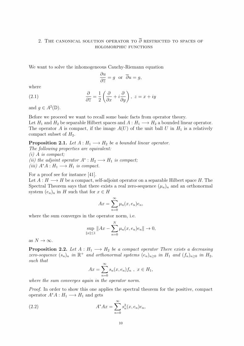
2. The canonical solution operator to ∂ restricted to spaces ofholomorphic functions

We want to solve the inhomogeneous Cauchy-Riemann equation

∂u

∂z= g or ∂u = g,

where

(2.1)∂

∂z=

1

2

(∂

∂x+ i

∂

∂y

), z = x+ iy

and g ∈ A2(D).

Before we proceed we want to recall some basic facts from operator theory.Let H1 and H2 be separable Hilbert spaces and A : H1 −→ H2 a bounded linear operator.The operator A is compact, if the image A(U) of the unit ball U in H1 is a relativelycompact subset of H2.

Proposition 2.1. Let A : H1 −→ H2 be a bounded linear operator.The following properties are equivalent:(i) A is compact;(ii) the adjoint operator A∗ : H2 −→ H1 is compact;(iii) A∗A : H1 −→ H1 is compact.

For a proof see for instance [41].Let A : H −→ H be a compact, self-adjoint operator on a separable Hilbert space H. TheSpectral Theorem says that there exists a real zero-sequence (µn)n and an orthonormalsystem (en)n in H such that for x ∈ H

Ax =∞∑n=0

µn(x, en)en,

where the sum converges in the operator norm, i.e.

sup‖x‖≤1

‖Ax−N∑n=0

µn(x, en)en‖ → 0,

as N →∞.

Proposition 2.2. Let A : H1 −→ H2 be a compact operator There exists a decreasingzero-sequence (sn)n in R+ and orthonormal systems (en)n≥0 in H1 and (fn)n≥0 in H2,such that

Ax =∞∑n=0

sn(x, en)fn , x ∈ H1,

where the sum converges again in the operator norm.

Proof. In order to show this one applies the spectral theorem for the positive, compactoperator A∗A : H1 −→ H1 and gets

(2.2) A∗Ax =∞∑n=0

s2n(x, en)en,

10

where s2n are the eigenvalues of A∗A. If sn > 0, we set fn = s−1

n Aen and get

(fn, fm) =1

snsm(Aen, Aem) =

1

snsm(A∗Aen, em) =

s2n

snsm(en, em) = δn,m.

For y ∈ H1 with y ⊥ en for each n ∈ N0 we have by (13.1) that

‖Ay‖2 = (Ay,Ay) = (A∗Ay, y) = 0.

Hence we have

Ax = A

(x−

∞∑n=0

(x, en)en

)+ A

(∞∑n=0

(x, en)en

)

=∞∑n=0

(x, en)Aen =∞∑n=0

sn(x, en)fn.

The numbers sn are uniquely determined by the operator A, they are the eigenvalues ofA∗A, and they are called the s-numbers of A.Let 0 < p <∞. the operator A belongs to the Schatten-class Sp, if its sequence (sn)n ofs-numbers belongs to lp. The elements of the Schatten class S2 are called Hilbert-Schmidtoperators. A is a Hilbert-Schmidt operator if and only if

∑∞n=0 ‖Aen‖2 < ∞ for each

complete orthonormal system (en)n in H.On L2-spaces Hilbert-Schmidt operators can be described in the following way:Let S ⊆ Rn and T ⊆ Rm be open sets and A : L2(T ) −→ L2(S) a linear mapping. A isa Hilbert-Schmidt operator if and only if there exists K ∈ L2(S × T ), such that

Af(s) =

∫T

K(s, t)f(t) dt , f ∈ L2(T ).

For the proof see for instance [41].The following characterization of compactness is useful for the special operators in thetext, see for instance [13]):

Proposition 2.3. Let H1 and H2 be Hilbert spaces, and assume that S : H1 → H2 is abounded linear operator. The following three statements are equivalent:

• S is compact.• For every ε > 0 there is a C = Cε > 0 and a compact operator T = Tε : H1 → H2

such that

(2.3) ‖Sv‖H2≤ C ‖Tv‖H2

+ ε ‖v‖H1.

• For every ε > 0 there is a C = Cε > 0 and a compact operator T = Tε : H1 → H2

such that

(2.4) ‖Sv‖2H2≤ C ‖Tv‖2

H2+ ε ‖v‖2

H1.

Proof. First we show that (13.2) and (13.3) are equivalent.Suppose that (13.3) holds. Write (13.3) with ε and C replaced by their squares to obtain

‖Sv‖2H2≤ C2 ‖Tv‖2

H2+ ε2 ‖v‖2

H1≤ (C ‖Tv‖H2

+ ε ‖v‖H1)2,

which implies (13.2).

11

Now suppose that (13.2) holds. Choose η with ε = 2η2 and apply (13.2) with ε replacedby η to get

‖Sv‖2H2≤ C2 ‖Tv‖2

H2+ 2ηC ‖v‖H1

‖Tv‖H2+ η2 ‖v‖2

H1.

It is easily seen (small constant - large constant trick) that there is C ′ > 0 such that

2ηC ‖v‖H1‖Tv‖H2

≤ η2 ‖v‖2H1

+ C ′ ‖Tv‖2H2,

hence

‖Sv‖2H2≤ (C2 + C ′) ‖Tv‖2

H2+ 2η2 ‖v‖2

H1= C ′′ ‖Tv‖2

H2+ ε ‖v‖2

H1.

To prove the lemma it therefore suffices to prove that (13.2) is equivalent to compactness.When S is known to be compact, we choose T = S and C = 1, and (13.2) holds for everypositive ε.For the converse let (vn)n be a bounded sequence in H1. We want to extract a Cauchysubsequence from (Svn)n. From (13.2) we have

(2.5) ‖Svn − Svm‖H2≤ C ‖Tvn − Tvm‖H2

+ ε ‖vn − vm‖H1

Given a positive integer N, we may choose ε sufficiently small in (13.4) so that the secondterm on the right-hand side is at most 1/(2N). The first term can be made smaller than1/(2N) by extracting a subsequence of (vn)n (still labeled the same) for which (Tvn)nconverges, and then choosing n and m large enough.

Let (v(0)n )n denote the original bounded sequence. The above argument shows that, for

each positive integer N, there is a sequence (v(N)n )n satisfying : (v

(N)n )n is a subsequence

of (v(N−1)n )n, and for any pair v and w in (v

(N)n )n we have ‖Sv − Sw‖H2

≤ 1/N.

Let (wk)k be the diagonal sequence defined by wk = v(k)k . Then (wk)k is a subsequence

of (v(0)n )n and the image sequence under S of (wk)k is a Cauchy sequence. Since H2 is

complete, the image sequence converges and S is compact.

We return to the inhomogeneous Cauchy-Riemann equation Let

(2.6) S(g)(z) =

∫DK(z, w)g(w)(z − w)−dλ(w).

Then we have

S(g)(z) = zg(z)− P (g)(z),

where P : L2(D) −→ A2(D) is the Bergman projection and g(w) = wg(w). We claimthat S(g) is a solution of the inhomogeneous Cauchy-Riemann equation:

∂

∂zS(g)(z) =

∂z

∂zg(z) + z

∂g

∂z+∂P (g)

∂z= g(z),

because g and P (g) are holomorphic functions, therefore ∂S(g) = g. In addition we haveS(g) ⊥ A2(D), because for arbitrary f ∈ A2(D) we get

(Sg, f) = (g − P (g), f) = (g, f)− (P (g), f) = (g, f)− (g, Pf) = (g, f)− (g, f) = 0.

The operator S : A2(D) −→ L2(D) is called the canonical solution operator to ∂.Now we want to show that S is a compact operator. For this purpose we consider theadjoint operator S∗ and prove that S∗S is compact, which implies that S is compact (forfurther details see [23]).

12

For g ∈ A2(D) and f ∈ L2(D) we have

(Sg, f) =

∫D

(∫DK(z, w)g(w)(z − w)− dλ(w)

)f(z) dλ(z)

=

∫D

(∫DK(w, z)(z − w)f(z) dλ(z)

)−g(w) dλ(w) = (g, S∗f)

hence

(2.7) S∗(f)(w) =

∫DK(w, z)(z − w)f(z) dλ(z).

Now set

c2n =

∫D|z|2n dλ(z) =

π

n+ 1,

and φn(z) = zn/cn , n ∈ N0, then the Bergman kernel K(z, w) can be expressed in theform

K(z, w) =∞∑k=0

zkwk

c2k

.

Next we compute

P (φn)(z) =

∫D

∞∑k=0

zkwk

c2k

wwn

cndλ(w) =

∞∑k=1

zk−1

c2k−1

∫D

wkwn

cndλ(w) =

cnzn−1

c2n−1

,

hence we have

S(φn)(z) = z φn(z)− cnzn−1

c2n−1

, n ∈ N.

Now we apply S∗ and get

S∗S(φn)(w) =

∫D

∞∑k=0

wkzk

c2k

(z − w)

(zzn

cn− cnz

n−1

c2n−1

)dλ(z).

The last integral is computed in two steps: first the multiplication by z∫D

∞∑k=0

wkzk

c2k

(zzn+1

cn− cnz

n

c2n−1

)dλ(z)

=

∫D

zn+1

cn

∞∑k=0

wkzk+1

c2k

dλ(z)− cnc2n−1

∫Dzn

∞∑k=0

wkzk

c2k

dλ(z)

=wn

c3n

∫D|z|2n+2 dλ(z)− wn

c2n−1cn

∫D|z|2n dλ(z)

=

(c2n+1

c3n

− cnc2n−1

)wn.

Next the multiplication by w

w

∫D

∞∑k=0

wkzk

c2k

(zzn

cn− cnz

n−1

c2n−1

)dλ(z)

13

= w

∫D

zn

cn

∞∑k=0

wkzk+1

c2k

dλ(z)− w∫D

cnzn−1

c2n−1

∞∑k=0

wkzk

c2k

dλ(z)

= w

(cnw

n−1

c2n−1

− cnwn−1

c2n−1

)= 0,

it follows that

S∗S(φn)(w) =

(c2n+1

c2n

− c2n

c2n−1

)φn(w) , n = 1, 2, . . . ,

for n = 0 an analogous computation shows

S∗S(φ0)(w) =c2

1

c20

φ0(w).

Finally we get

Proposition 2.4. Let S : A2(D) −→ L2(D) be the canonical solution operator for ∂ and(φk)k the normalized monomials. Then

(2.8) S∗Sφ =c2

1

c20

(φ, φ0)φ0 +∞∑n=1

(c2n+1

c2n

− c2n

c2n−1

)(φ, φn)φn

for each φ ∈ A2(D).

Sincec2n+1

c2n

− c2n

c2n−1

=1

(n+ 2)(n+ 1)→ 0 as n→∞,

it follows that S∗S is compact and S too.

We have also shown that the s-numbers of S are(c2n+1

c2n− c2n

c2n−1

)1/2

and since

∞∑n=0

(c2n+1

c2n

− c2n

c2n−1

)<∞

it follows that S is Hilbert-Schmidt.This can also be shown directly. For this purpose we claim that the function (z, w) 7→K(z, w)(z − w)− belongs to L2(D× D).We have to prove, that ∫

D

∫D

|z − w|2

|1− zw|4dλ(z) dλ(w) <∞.

An easy estimate gives |z − w| ≤ |1− zw|, for z, w ∈ D. Hence∫D

∫D

|z − w|2

|1− zw|4dλ(z) dλ(w) ≤

∫D

∫D

1

|1− zw|2dλ(z) dλ(w).

Introducing polar coordinates z = r eiθ and w = s eiφ we can write the last integral inthe following form∫

D

∫D

1

|1− zw|2dλ(z) dλ(w) =

∫ 1

0

∫ 1

0

∫ 2π

0

∫ 2π

0

r s dθ dφ dr ds

1− 2 r s cos(θ − φ) + r2 s2

14

=

∫ 1

0

∫ 1

0

∫ 2π

0

∫ 2π

0

1− r2 s2

1− 2 r s cos(θ − φ) + r2 s2

r s

1− r2 s2dθ dφ dr ds.

Integration of the Poisson kernel with respect to θ yields∫ 2π

0

1− ρ2

1− 2ρ cos(θ − φ) + ρ2dθ = 2π , 0 < ρ < 1.

Therefore we have∫ 1

0

∫ 1

0

∫ 2π

0

∫ 2π

0

1− r2 s2

1− 2 r s cos(θ − φ) + r2 s2

r s

1− r2 s2dθ dφ dr ds

= (2π)2

∫ 1

0

∫ 1

0

r s

1− r2 s2dr ds = − (2π)2

∫ 1

0

log(1− s2)

2sds <∞.

For further details see [23], [27] and [37].

Now we consider weighted spaces on entire functions

A2(C, e−|z|m) = f : C −→ C : ‖f‖2m :=

∫C|f(z)|2 e−|z|m dλ(z) <∞,

where m > 0. Let

c2k =

∫C|z|2k e−|z|m dλ(z).

Then

Km(z, w) =∞∑k=0

zkwk

c2k

is the reproducing kernel for A2(C, e−|z|m).In the sequel the expression

c2k+1

c2k

− c2k

c2k−1

will become important. Using the integral representation of the Γ−function one easilysees that the above expression is equal to

Γ(

2k+4m

)Γ(

2k+2m

) − Γ(

2k+2m

)Γ(

2km

) .

For m = 2 this expression equals to 1 for each k = 1, 2, . . . . We will be interested in thelimit behavior for k → ∞. By Stirlings formula the limit behavior is equivalent to thelimit behavior of the expression(

2k + 2

m

)2/m

−(

2k

m

)2/m

,

as k →∞. Hence we have shown the following

Lemma 2.5. The expression

Γ(

2k+4m

)Γ(

2k+2m

) − Γ(

2k+2m

)Γ(

2km

)15

tends to ∞ for 0 < m < 2, is equal to 1 for m = 2 and tends to zero for m > 2 as ktends to ∞.

Let 0 < ρ < 1, define fρ(z) := f(ρz) and fρ(z) = zfρ(z), for f ∈ A2(C, e−|z|m). Then it

is easily seen that fρ ∈ L2(C, e−|z|m), but there are functions g ∈ A2(C, e−|z|m) such thatzg 6∈ L2(C, e−|z|m).Let Pm : L2(C, e−|z|m) −→ A2(C, e−|z|m) denote the orthogonal projection. Then Pm canbe written in the form

Pm(f)(z) =

∫CKm(z, w)f(w)e−|w|

m

dλ(w) , f ∈ L2(C, e−|z|m).

Proposition 2.6. Let m ≥ 2. Then there is a constant Cm > 0 depending only on msuch that ∫

C

∣∣∣fρ(z)− Pm(fρ)(z)∣∣∣2 e−|z|m dλ(z) ≤ Cm

∫C|f(z)|2e−|z|m dλ(z),

for each 0 < ρ < 1 and for each f ∈ A2(C, e−|z|m).

Proof. First we observe that for the Taylor expansion of f(z) =∑∞

k=0 akzk we have

Pm(fρ)(z) =

∫C

∞∑k=0

zkwk

c2k

(w∞∑j=0

ajρjwj

)e−|w|

m

dλ(w)

=∞∑k=1

akc2k

c2k−1

ρkzk−1.

Now we obtain ∫C

∣∣∣fρ(z)− Pm(fρ)(z)∣∣∣2 e−|z|m dλ(z)

=

∫C

(z∞∑k=0

akρkzk −

∞∑k=1

akc2k

c2k−1

ρkzk−1

)

×

(z

∞∑k=0

akρkzk −

∞∑k=1

akc2k

c2k−1

ρkzk−1

)e−|z|

m

dλ(z)

=

∫C(∞∑k=0

|ak|2ρ2k|z|2k+2 − 2∞∑k=1

|ak|2c2k

c2k−1

ρ2k|z|2k

+∞∑k=1

|ak|2c4k

c4k−1

ρ2k|z|2k−2) e−|z|m

dλ(z)

= |a0|2 c21 +

∞∑k=1

|ak|2 c2k ρ

2k

(c2k+1

c2k

− c2k

c2k−1

).

Now the result follows from the fact that∫C|f(z)|2e−|z|m dλ(z) =

∞∑k=0

|ak|2 c2k,

and that the sequence(c2k+1

c2k− c2k

c2k−1

)k

is bounded.

16

Remark 2.7. Already in the last Proposition the sequence(c2k+1

c2k− c2k

c2k−1

)k

plays an im-

portant role and it will turn out that this sequence is the sequence of eigenvalues of theoperator S∗mSm (see below).

Proposition 2.8. Let m ≥ 2 and consider an entire function f ∈ A2(C, e−|z|m) withTaylor series expansion f(z) =

∑∞k=0 akz

k. Let

F (z) := z

∞∑k=0

akzk −

∞∑k=1

akc2k

c2k−1

zk−1

and define Sm(f) := F. Then Sm : A2(C, e−|z|m) −→ L2(C, e−|z|m) is a continuous linearoperator, representing the canonical solution operator to ∂ restricted to A2(C, e−|z|m), i.e.∂Sm(f) = f and Sm(f) ⊥ A2(C, e−|z|m).

Proof. By the proof of Proposition 2.6, by Abel’s theorem and by Fatou’s theorem (seefor instance [15]) we have∫

C|F (z)|2e−|z|m dλ(z) =

∫C

limρ→1

∣∣∣fρ(z)− Pm(fρ)(z)∣∣∣2 e−|z|m dλ(z)

≤ sup0<ρ<1

∫C

∣∣∣fρ(z)− Pm(fρ)(z)∣∣∣2 e−|z|m dλ(z)

≤ Cm

∫C|f(z)|2e−|z|m dλ(z)

and hence the function

F (z) := z∞∑k=0

akzk −

∞∑k=1

akc2k

c2k−1

zk−1

belongs to L2(C, e−|z|m) and satisfies

(2.9)

∫C|F (z)|2e−|z|m dλ(z) ≤ Cm

∫C|f(z)|2e−|z|m dλ(z).

The above computation also shows that limρ→1 ‖fρ − Pm(fρ)‖m = ‖F‖m and by a stan-dard argument for Lp-spaces (see for instance [15])

limρ→1‖fρ − Pm(fρ)− F‖m = 0.

A similar computation as in the case A2(D) shows that the function F defined abovesatisfies ∂F = f. Let Sm(f) := F. Then, by the last remarks, Sm : A2(C, e−|z|m) −→L2(C, e−|z|m) is a continuous linear solution operator for ∂. For arbitrary h ∈ A2(C, e−|z|m)we have

(h, Sm(f))m = (h, F )m = limρ→1

(h, fρ − Pm(fρ))m = limρ→1

(h− Pm(h), fρ)m = 0,

where (. , .)m denotes the inner product in L2(C, e−|z|m). Hence Sm is the canonical solu-tion operator for ∂ restricted to A2(C, e−|z|m).

Remark 2.9. Let

f(z) =∞∑k=0

zk√(k + 1)!

√k + 1

.

17

Then f ∈ A2(C, e−|z|2), since

‖f‖22 = 2π

∞∑k=0

k!

(k + 1)!(k + 1)= 2π

∞∑k=0

1

(k + 1)2<∞.

But

‖zf‖22 = 2π

∞∑k=0

(k + 1)!

(k + 1)!(k + 1)= 2π

∞∑k=0

1

(k + 1)=∞,

hence zf 6∈ L2(C, e−|z|2).The expression for the function F in the last theorem corresponds formally to the ex-pression zf − Pm(zf); in general zf 6∈ L2(C, e−|z|m), for f ∈ A2(C, e−|z|m), but f 7→ Fdefines a bounded linear operator from A2(C, e−|z|m) to L2(C, e−|z|m).

Theorem 2.10. The canonical solution operator to ∂ restricted to the space A2(C, e−|z|m)is compact if and only if

limk→∞

(c2k+1

c2k

− c2k

c2k−1

)= 0.

Proof. For a complex polynomial p the canonical solution operator Sm can be written inthe form

Sm(p)(z) =

∫CKm(z, w)p(w)(z − w)e−|w|

m

dλ(w),

therefore we can express the conjugate S∗m in the form

S∗m(q)(w) =

∫CKm(w, z)q(z)(z − w)e−|z|

m

dλ(z),

if q is a finite linear combination of the terms zk zl. This follows by considering the innerproduct (Sm(p), q)m = (p, S∗m(q))m.Now we claim that

S∗mSm(un)(w) =

(c2n+1

c2n

− c2n

c2n−1

)un(w) , n = 1, 2, . . .

and

S∗mSm(u0)(w) =c2

1

c20

u0(w),

where un(z) = zn/cn, n = 0, 1, . . . is the standard orthonormal basis of A2(C, e−|z|m).In a similar way as before for the case of A2(D) we see that

Sm(un)(z) = zun(z)− cnzn−1

c2n−1

, n = 1, 2, . . . .

Hence

S∗mSm(un)(w) =

∫CKm(w, z)(z − w)

(zzn

cn− cnz

n−1

c2n−1

)e−|z|

m

dλ(z)

=

∫C

∞∑k=0

wkzk

c2k

(z − w)

(zzn

cn− cnz

n−1

c2n−1

)e−|z|

m

dλ(z).

As before we get∫C

∞∑k=0

wkzk

c2k

(zzn+1

cn− cnz

n

c2n−1

)e−|z|

m

dλ(z) =

(c2n+1

c3n

− cnc2n−1

)wn

18

and

w

∫C

∞∑k=0

wkzk

c2k

(zzn

cn− cnz

n−1

c2n−1

)e−|z|

m

dλ(z) = w

(cnw

n−1

c2n−1

− cnwn−1

c2n−1

)= 0,

which implies that

S∗mSm(un)(w) =

(c2n+1

c2n

− c2n

c2n−1

)un(w) , n = 1, 2, . . . ,

the case n = 0 follows from an analogous computation.The last statement says that S∗mSm is a diagonal operator with respect to the orthonormalbasis un(z) = zn/cn of A2(C, e−|z|m). Therefore it is easily seen that S∗mSm is compactif and only if

limn→∞

(c2n+1

c2n

− c2n

c2n−1

)= 0.

Theorem 2.11. The canonical solution operator for ∂ restricted to the space A2(C, e−|z|m)

is compact, if m > 2. The canonical solution operator for ∂ as operator from L2(C, e−|z|2)into itself is not compact.

Proof. The first statement follows immediately from Theorem 2.10 and Lemma 2.5 Forthe second statement we use (2.9) to show that the canonical solution operator is con-

tinuous as operator from A2(C, e−|z|2) to L2(C, e−|z|2).By Hormander’s L2-estimate for the solution of the ∂ equation [30] there is for each

g ∈ L2(C, e−|z|2) a function f ∈ L2(C, e−|z|2) such that ∂f = g and

∫C|f(z)|2 e−|z|2 dλ(z) ≤ 2

∫C|g(z)|2 e−|z|2 dλ(z).

(see section 7. Theorem 7.5)

Hence the canonical solution operator for ∂ as operator from L2(C, e−|z|2) into itself is

continuous and its restriction to the closed subspace A2(C, e−|z|2) fails to be compact byPropositon 2.6 and Lemma 2.5. By the definition of compactness this implies that thecanonical solution operator is not compact as operator from L2(C, e−|z|2) into itself.

Remark 2.12. In the case of the Fock space A2(C, e−|z|2) the composition S∗2S2 equals

to the identity on A2(C, e−|z|2), which follows from the proof of Theorem 2.10.

Theorem 2.13. Let m ≥ 2. The canonical solution operator for ∂ restricted to A2(C, e−|z|m)fails to be Hilbert Schmidt.

19

Proof. By Proposition 2.8 we know that the canonical solution operator is continuousand we can use the techniques from before to get

‖Sm(un)‖2m =

1

c2n

∫C

∣∣∣∣z zn − c2n

c2n−1

zn−1

∣∣∣∣2 e−|z|m dλ(z)

=1

c2n

∫C|z|2n−2

(|z|4 − 2c2

n|z|2

c2n−1

+c4n

c4n−1

)e−|z|

m

dλ(z)

=1

c2n

∫C|z|2n+2 e−|z|

m

dλ(z)− 2

c2n−1

∫C|z|2n e−|z|m dλ(z)

+c2n

c4n−1

∫C|z|2n−2 e−|z|

m

dλ(z)

=c2n+1

c2n

− c2n

c2n−1

.

Hence∞∑n=0

‖Sm(un)‖2m <∞

if and only if

limn→∞

c2n+1

c2n

<∞.

By [41] , 16.8, Sm is a Hilbert Schmidt operator if and only if∞∑n=0

‖Sm(un)‖2m <∞.

(see Appendix A.)In our case we have

c2n+1

c2n

= Γ

(2n+ 4

m

)/Γ

(2n+ 2

m

),

which, by Stirling’s formula, implies that the corresponding canonical solution operatorto ∂ fails to be Hilbert Schmidt.

In the case of several variables the corresponding operator S∗S is more complicated,nevertheless, using a suitable orthogonal decomposition, we can generalize the aboveresults, see next section.

20

3. Spectral properties of the canonical solution operator to ∂

In this chapter we concentrate on several complex variables and follow [27] to generalizethe results of chapter 1 and 2.For this purpose we introduce the notion of complex differential forms. Let Ω ⊆ Cn bean open subset and f : Ω −→ C be a C1-function. We write zj = xj + iyj and considerfor P ∈ Ω the differential

dfP =n∑j=1

(∂f

∂xj(P ) dxj +

∂f

∂yj(P ) dyj

).

We use the complex differentials

dzj = dxj + idyj , dzj = dxj − idyjand the derivatives

∂

∂zj=

1

2

(∂

∂xj− i ∂

∂yj

),

∂

∂zj=

1

2

(∂

∂xj+ i

∂

∂yj

)and rewrite the differential dfp in the form

dfP =n∑j=1

(∂f

∂zj(P ) dzj +

∂f

∂zj(P ) dzj

)= ∂fP + ∂fP .

A general differential form is given by

ω =∑

|J |=p,|K|=q

′ aJ,K dzJ ∧ dzK ,

where the sum is taken only over increasing multiindices J = (j1, . . . , jp), K = (k1, . . . , kq)and

dzJ = dzj1 ∧ · · · ∧ dzjp , dzK = dzk1 ∧ · · · ∧ dzkq .The derivative dω of ω is defined by

dω =∑

|J |=p,|K|=q

′ daJ,K ∧ dzJ ∧ dzK =∑

|J |=p,|K|=q

′ (∂aJ,K + ∂aJ,K) ∧ dzJ ∧ dzK ,

and we set

∂ω =∑

|J |=p,|K|=q

′ ∂aJ,K ∧ dzJ ∧ dzK and ∂ω =∑

|J |=p,|K|=q

′ ∂aJ,K ∧ dzJ ∧ dzK .

We have d = ∂ + ∂ and since d2 = 0 it follows that

0 = (∂ + ∂) (∂ + ∂)ω = (∂ ∂)ω + (∂ ∂ + ∂ ∂)ω + (∂ ∂)ω,

which implies ∂2 = 0 , ∂2

= 0 and ∂ ∂ + ∂ ∂ = 0, by comparing the types of thedifferential forms involved.

Let Ω be a bounded domain in Cn and let A2(0,1)(Ω) denote the space of all (0, 1)-forms

with holomorphic coefficients belonging to L2(Ω). With the same proof as in section 2one shows that the canonical solution operator S : A2

(0,1)(Ω) −→ L2(Ω) has the form

(3.1) S(g)(z) =

∫Ω

K(z, w) < g(w), z − w > dλ(w),

21

where K denotes the Bergman kernel of Ω and

< g(w), z − w >=n∑j=1

gj(w)(zj − wj),

for z = (z1, . . . , zn) and w = (w1, . . . , wn).

Let v(z) =∑n

j=1 zjgj(z). Then it follows that

∂v =n∑j=1

∂v

∂zjdzj =

n∑j=1

gjdzj = g.

Hence the canonical solution operator S1 can be written in the form S1(g) = v − P (v),where P : L2(Ω) −→ A2(Ω) is the Bergman projection. If v is another solution to ∂u = g,then v − v ∈ A2(Ω) hence v = v + h, where h ∈ A2(Ω). Therefore

v − P (v) = v + h− P (v)− P (h) = v − P (v).

Since gj ∈ A2(Ω), j = 1, . . . , n, we have

gj(z) =

∫Ω

K(z, w)gj(w) dλ(w).

Now we get

S(g)(z) =n∑j=1

zjgj(z)−∫

Ω

K(z, w)

(n∑j=1

wjgj(w)

)dλ(w)

=

∫Ω

[(n∑j=1

zjgj(w)

)K(z, w)−

(n∑j=1

wjgj(w)

)K(z, w)

]dλ(w)

=

∫Ω

K(z, w) < g(w), z − w > dλ(w).

Remark 3.1. It is pointed out that a (0, 1)-form g =∑n

j=1 gj dzj with holomorphic

coefficients is not invariant under the pull back by a holomorphic map F = (F1, . . . , Fn) :Ω1 −→ Ω. Then

F ∗g =n∑l=1

gl dF l =n∑j=1

(n∑l=1

gl∂F l

∂zj

)dzj,

where we used the fact that

dF l = ∂F l + ∂ F l =n∑j=1

∂F l

∂zjdzj +

n∑j=1

∂F l

∂zjdzj =

n∑j=1

∂F l

∂zjdzj.

The expressions ∂F l∂zj

are not holomorphic.

Nevertheless it is true that ∂u = g implies ∂(u F ) = F ∗g, which follows from the factthat for a general differential form ω and a holomorphic map F we have

∂(F ∗ω) = F ∗(∂ω) and ∂(F ∗ω) = F ∗(∂ω).

22

Now let ω be a holomorphic (n, n)-form, i.e.

ω = ω dz1 ∧ · · · ∧ dzn ∧ dz1 ∧ · · · ∧ dzn,where ω ∈ A2(Ω). In this case we can express the canonical solution to ∂u = ω in thefollowing form

Proposition 3.2. Let u be the (n, n− 1)-form

u =n∑j=1

uj dz1 ∧ · · · ∧ dzn ∧ dz1 ∧ · · · ∧ [dzj] ∧ · · · ∧ dzn,

where

uj(z) =(−1)n+j−1

n

∫Ω

(zj − wj)K(z, w)ω(w) dλ(w).

Then uj ⊥ A2(Ω) , j = 1, . . . , n and ∂u = ω.

Proof. It follows that

uj(z) =(−1)n+j−1

n(zjω(z)− P (wjω)(z)) ,

from this we obtain

∂uj∂zk

=(−1)n+j−1

n

(∂zj∂zk

ω + zj∂ω

∂zk

)=

(−1)n+j−1

nδjk ω,

where δjk is the Kronecker delta symbol. Hence

∂u =n∑k=1

n∑j=1

∂uj∂zk

dzk ∧ dz1 ∧ · · · ∧ dzn ∧ dz1 ∧ · · · ∧ [dzj] ∧ · · · ∧ dzn

=n∑k=1

n∑j=1

((−1)n+j−1/n

)δjk ω dzk ∧

∧dz1 ∧ · · · ∧ dzn ∧ dz1 ∧ · · · ∧ [dzj] ∧ · · · ∧ dzn= ω dz1 ∧ · · · ∧ dzn ∧ dz1 ∧ · · · ∧ dzn.

Remark 3.3. The pull back by a holomorphic map F has in this case the form

F ∗ω =

∣∣∣∣det∂Fj∂zk

∣∣∣∣2 ω dz1 ∧ · · · ∧ dzn ∧ dz1 ∧ · · · ∧ dzn.

For further related results see section 10.

Now we will study boundedness, compactness, and Schatten-class membership of thecanonical solution operator to ∂, restricted to (0, 1)-forms with holomorphic coefficients,on L2(dµ) where µ is a measure with the property that the monomials form an orthogonalfamily in L2(dµ). The characterizations are formulated in terms of moment propertiesof µ.This situation covers a number of basic examples:

23

• Lebesgue measure on bounded domains in Cn which are invariant under the torusaction

(θ1, . . . , θn)(z1, . . . , zn) 7→ (eiθ1z1, . . . eiθnzn)

(i.e. Reinhardt domains).• Weighted L2 spaces with radially symmetric weights (e.g., generalized Fock spaces).• Weighted L2 spaces with decoupled radial weights, that is,

dµ = e∑j ϕj(|zj |2)dλ,

where ϕj : R→ R is a weight function.

We denote by

A2(dµ) = zα : α ∈ Nn,the closure of the monomials in L2(dµ), and write

mα = c−1α =

∫|zα|2dµ.

We will give necessary and sufficient conditions in terms of these multimoments of themeasure µ for the canonical solution operator to ∂, when restricted to (0, 1)-forms withcoefficients in A2(dµ) to be bounded, compact, and to belong to the Schatten class Sp.This is accomplished by presenting a complete diagonalization of the solution operatorby orthonormal bases with corresponding estimates.As usual, for a given function space F , F(0,1) denotes the space of (0, 1)-forms withcoefficients in F , that is, expressions of the form

n∑j=0

fjdzj, fj ∈ F .

The ∂ operator is the densely defined operator

(3.2) ∂f =n∑j=1

∂f

∂zjdzj.

The canonical solution operator S assigns to each ω ∈ L2(0,1)(dµ) the solution to the ∂

equation which is orthogonal to A2(dµ); this solution need not exist, but if the ∂ equationfor ω can be solved, then Sω is defined, and is given by the unique f ∈ L2(dµ) whichsatisfies

∂f = ω in the sense of distributions and f ⊥ A2(dµ).

We will frequently encounter multiindices γ which might have one (but not more thanone) entry equal to −1: in that case, we define cγ = 0. We will denote the set of thesemultiindices by Γ. We let ej = (0, · · · , 1, · · · , 0) be the multiindex with a 1 in the jthspot and 0 elsewhere.

Theorem 3.4. S : A2(0,1)(dµ)→ L2(dµ) is bounded if and only if there exists a constant

C such thatcγ+ej

cγ+2ej

− cγcγ+ej

< C

for all multiindices γ ∈ Γ and for all j = 1, . . . , n.

We have a similar criterion for compactness:

24

Theorem 3.5. S : A2(0,1)(dµ)→ L2(dµ) is compact if and only if

(3.3) limγ

(cγ+ej

cγ+2ej

− cγcγ+ej

)= 0

for all j = 1, · · · , n.

In particular, the only if implication of Theorem 3.5 implies several known noncompact-ness statements for S, e.g. [34], [44], as well as the noncompactness of S on the polydisc.The main interest in these noncompactness statements is that if S fails to be compact,so does the ∂-Neumann operator N .The multimoments also lend themselves to characterizing the finer spectral property ofbeing in the Schatten class Sp. Let us recall that an operator T : H1 → H2 belongsto the Schatten-class Sp if the self-adjoint operator T ∗T has a sequence of eigenvaluesbelonging to `p.

Theorem 3.6. Let p > 0. Then S : A2(0,1)(dµ)→ L2(dµ) is in the Schatten-p-class Sp if

and only if

(3.4)∑γ∈Γ

(∑j

(cγ+ej

cγ+2ej

− cγcγ+ej

)) p2

<∞

The condition above is substantially easier to check if p = 2 (we will show that the sumis actually a telescoping sum then), i.e. for the case of the Hilbert-Schmidt class; westate this as a Theorem:

Theorem 3.7. The canonical solution operator S is in the Hilbert-Schmidt class if andonly if

(3.5) limk→∞

∑γ∈Nn,|γ|=k

1≤j≤n

cγcγ+ej

<∞.

Let us apply Theorem 3.4 to the case of decoupled weights, or more generally, of productmeasures dµ = dµ1 × · · · × dµn, where each dµk is a (circle-invariant) measure on C.Note that for such measures, there is definitely no compactness by Theorem 3.5. If wedenote by

ckj =

(∫C|z|2kdµj

)−1

,

we have that

c(γ1,··· ,γn) =n∏j=1

cγjj .

We thus obtain the following corollary.

Corollary 3.8. For a product measure dµ = dµ1 × · · · × dµn as above, the canonicalsolution operator S : A2

(0,1)(dµ)→ L2(dµ) is bounded if and only if there exists a constantC such that

ck+1j

ck+2j

−ckj

ck+1j

< C

for all k ∈ N0 and for all j = 1, · · · , n. Equivalently, S is bounded if and only if thecanonical solution operator Sj : A2(dµj)→ L2(dµj) is bounded for every j = 1, · · · , n.

25

To see that (3.3) is not satisfied for product measures consider multiindices γ ∈ Γ suchthat γj = −1 : then cγ = 0 (by definition) and cγ+ej 6= 0, and therefore(

cγ+ej

cγ+2ej

− cγcγ+ej

)=c0j

c1j

− 0 > δ > 0,

for all multiindices γ with γj = −1.

In the case of a rotation-invariant measure µ, we write

md =

∫Cn|z|2ddµ;

a computation (see Appendix F and [37, Lemma 2.1]) implies that

(3.6) cγ =(n+ |γ| − 1)!

(n− 1)!γ!

1

m|γ|,

where |γ| = γ1 + · · ·+ γn and γ! = γ1! . . . γn!.In order to express the conditions of our Theorems, we compute (setting d = |γ|+ 1)

(3.7)∑j

(cγ+ej

cγ+2ej

− cγcγ+ej

)=

d+2n−1d+n

md+1

md− md

md−1γj 6= −1 for all j

1d+n

md+1

mdelse.

Note that the Cauchy-Schwarz inequality implies that the first case in (3.7) always dom-inates the second case for n ≥ 2; for n = 1 we observe that the second case in (3.7)reduces to m1

m0, compare with Proposition 2.4.

Using this observation and some trivial inequalities, we get the following Corollaries.

Corollary 3.9. Let µ be a rotation invariant measure on Cn. Then the canonical solutionoperator to ∂ is bounded on A2

(0,1)(dµ) if and only if

(3.8) supd∈N

((2n+ d− 1)md+1

(n+ d)md

− md

md−1

)<∞

Corollary 3.10. Let µ be a rotation invariant measure on Cn. Then the canonicalsolution operator to ∂ is compact on A2

(0,1)(dµ) if and only if

(3.9) limd→∞

((2n+ d− 1)md+1

(n+ d)md

− md

md−1

)= 0.

Corollary 3.11. Let µ be a rotation invariant measure on Cn. Then the canonicalsolution operator to ∂ is a Hilbert-Schmidt operator on A2

(0,1)(dµ) if and only if

(3.10) limd→∞

(n+ d− 2

n− 1

)md+1

md

<∞.

Remark 3.12. It follows that the canonical solution operator to ∂ is a Hilbert-Schmidtoperator on A2(D), but fails to be Hilbert-Schmidt on A2(Bn), where Bn is the unit ballin Cn, for n ≥ 2.

Corollary 3.13. Let µ be a rotation invariant measure on Cn, p > 0. Then the canonicalsolution operator to ∂ is in the Schatten-class Sp, as an operator from A2

(0,1)(dµ) to L2(dµ)if and only if

(3.11)∞∑d=1

(n+ d− 2

n− 1

)((2n+ d− 1)md+1

(n+ d)md

− md

md−1

) p2

<∞.

26

In particular, Corollary 3.13 improves Theorem C of [37] in the sense that it also coversthe case 0 < p < 2. We would like to note that our techniques can be adapted to thesetting of [37] by considering the canonical solution operator on a Hilbert space H ofholomorphic functions endowed with a norm which is comparable to the L2-norm on eachsubspace generated by monomials of a fixed degree d, if in addition to the requirementsin [37] we also assume that the monomials belong to H; this introduces the additionalweights found by [37] in the formulas, as the reader can check. In our setting, theformulas are somewhat “cleaner” by working with A2(dµ) (in particular, Corollary 3.11only holds in this setting).

In what follows, we will denote by

uα =√cαz

α

the orthonormal basis of monomials for the space A2(dµ), and by Uα,j = uαdzj thecorresponding basis of A2

(0,1)(dµ). We first note that it is always possible to solve the

∂-equation for the elements of this basis; indeed, ∂zjuα = Uα,j. The canonical solutionoperator is also easily determined for forms with monomial coefficients:

Lemma 3.14. The canonical solution Szαdzj for monomial forms is given by

(3.12) Szαdzj = zjzα −

cα−ejcα

zα−ej , α ∈ Nn0 .

Proof. We have 〈zjzα, zβ〉 = 〈zα, zβ+ej〉; so this expression is nonzero only if β = α − ej(in particular, if this implies (3.12) for multiindices α with αj = 0; recall our conventionthat cγ = 0 if one of the entries of γ is negative). Thus Szαdzj = zjz

α + czα−ej , and c iscomputed by

0 = 〈zjzα + czα−ej , zα−ej〉 = c−1α + cc−1

α−ej ,

which gives c = −cα−ej/cα.

We are going to introduce an orthogonal decomposition

A2(0,1)(dµ) =

⊕γ∈Γ

Eγ

of A2(0,1)(dµ) into at most n-dimensional subspaces Eγ indexed by multiindices γ ∈ Γ (we

will describe the index set below), and a corresponding sequence of mutually orthogonalfinite-dimensional subspaces Fγ ⊂ L2(dµ) which diagonalizes S (by this we mean thatSEγ = Fγ). To motivate the definition of Eγ, note that

(3.13) 〈Szαdzk, Szβdz`〉 =

0 β 6= α + e` − ek,1cα

(cα

cα+e`− cα−ek

cα+e`−ek

)β = α + e` − ek,

so that 〈Szαdzk, Szβdz`〉 6= 0 if and only if there exists a multiindex γ such that α = γ+ekand β = γ + e`. We thus define

Eγ = spanUγ+ej ,j : 1 ≤ j ≤ n

= span

zγ+ejdzj : 1 ≤ j ≤ n

,

and likewise Fγ = SEγ. Recall that Γ is defined to be the set of all multiindices whoseentries are greater or equal to −1 and at most one negative entry. Note that Eγ is 1-dimensional if exactly one entry in γ equals −1, and n-dimensional otherwise. We havealready observed that Fγ are mutually orthogonal subspaces of L2(dµ) (see 3.13).

27

Whenever we use multiindices γ and integers p ∈ 1, · · · , n as indices, we use theconvention that the p run over all p such that γ + ep ≥ 0; that is, for a fixed multiindexγ ∈ Γ, either the indices are either all p ∈ 1, · · · , n or there is exactly one p such thatγp = −1, in which case the index is exactly this one p.We next observe that we can find an orthonormal basis of Eγ and an orthonormal basisof Fγ such that in these bases Sγ = S|Eγ : Eγ → Fγ acts diagonally. First note that itis enough to do this if dimEγ = n (since an operator between one-dimensional spaces isautomatically diagonal). Fixing γ, the functions Uj := Uγ+ej ,j are an orthonormal basisof Eγ. The operator Sγ is clearly nonsingular on this space, so the functions SUj = Ψj

constitute a basis of Fγ. For a basis B of vectors vj =(vj1, . . . , v

jn

), j = 1, . . . , n of Cn

we consider the new basis

Vk =n∑j=1

vjkUj;

since the basis given by the Uj is orthonormal, the basis given by the Vk is also orthonor-mal provided that the vectors vk = (v1

k, · · · , vnk ) constitute an orthonormal basis for Cn

with the standard hermitian product. Let us write

Φk = SVk =∑j

vjkSUj.

The inner product 〈Φp,Φq〉 is then given by∑

j,k vjpvkq 〈SUj, SUk〉. We therefore have

(3.14)

〈Φ1,Φ1〉 · · · 〈Φ1,Φn〉...

...〈Φn,Φ1〉 · · · 〈Φn,Φn〉

=

v11 · · · vn1...

...v1n · · · vnn

〈Ψ1,Ψ1〉 · · · 〈Ψ1,Ψn〉...

...〈Ψn,Ψ1〉 · · · 〈Ψn,Ψn〉

v11 · · · v1

n...

...vn1 vnn

.

Since the matrix (〈Ψj,Ψk〉)j,k is hermitian, we can unitarily diagonalize it; that is, we canchoose an orthnormal basis B of Cn such that with this choice of B the vectors ϕγ,k =

Vk =∑

j vjkUγ+ej ,j of Eγ are orthonormal, and their images Φk = SVk are orthogonal in

Fγ. Therefore, Φk/‖Φk‖ is an orthonormal basis of Fγ such that Sγ : Eγ → Fγ is diagonalwhen expressed in terms of the bases V1, · · · , Vn ⊂ Eγ and Φ1, · · · ,Φn ⊂ Fγ, withentries ‖Φk‖.Furthermore, the ‖Φk‖ are exactly the square roots of the eigenvalues of the matrix(〈Ψp,Ψq〉) which by (3.13) is given by

(3.15)

〈Ψp,Ψq〉 = 〈SUγ+ep,p, SUγ+eq ,q〉=√cγ+ep

√cγ+eq〈S zγ+ep dzp, S z

γ+eq dzq〉

=√cγ+epcγ+eq

1

cγ+ep

(cγ+ep

cγ+ep+eq

− cγcγ+eq

)=cγ+epcγ+eq − cγcγ+ep+eq

cγ+ep+eq√cγ+epcγ+eq

Summarizing, we have the following Proposition.

28

Proposition 3.15. With µ as above, the canonical solution operator S : A2(0,1)(dµ) →

L2(0,1)(dµ) admits a diagonalization by orthonormal bases. In fact, we have a decomposi-

tion A2(0,1) =

⊕γ Eγ into mutually orthogonal finite dimensional subspaces Eγ, indexed by

the multiindices γ with at most one negative entry (equal to −1), which are of dimension1 or n, and orthonormal bases ϕγ,j of Eγ, such that Sϕγ,j is a set of mutually orthogonalvectors in L2(dµ). For fixed γ, the norms ‖Sϕγ,j‖ are the square roots of the eigenvaluesof the matrix Cγ = (Cγ,p,q)p,q given by

(3.16) Cγ,p,q =cγ+epcγ+eq − cγcγ+ep+eq

cγ+ep+eq√cγ+epcγ+eq

.

In particular, we have that

(3.17)n∑j=1

‖Sϕγ,j‖2 = tr(Cγ,p,q)p,q =n∑p=1

(cγ+ep

cγ+2ep

− cγcγ+ep

)

In order to prove Theorem 3.4, we are using Proposition 3.15. We have seen that wehave an orthonormal basis ϕγ,j, γ ∈ Γ, j ∈ 1, · · · , n, such that the images Sϕγ,j aremutually orthogonal. Thus, S is bounded if and only if there exists a constant C suchthat

‖Sϕγ,j‖2 ≤ C

for all γ ∈ Γ and j ∈ 1, · · · , dimEγ. If dimEγ = 1, then γ has exactly one entry(say the jth one) equal to −1; in that case, let us write ϕγ = Uγ+ejdzj. We haveSϕγ =

√cγ+ej zjz

γ+ej , and so

‖Sϕγ‖2 =cγ+ej

cγ+2ej

.

On the other hand, if dimEγ = n, we argue as follows: Writing ‖Sϕγ,j‖2 = λ2γ,j with

λγ,j > 0, from (3.17) we find that

n∑j=1

λ2γ,j =

n∑j=1

(cγ+ej

cγ+2ej

− cγcγ+ej

).

The last 2 equations complete the proof of Theorem 3.4.

In order to prove Theorem 3.5, we use a special characterization of compactness, for theproof see Appendix A.

Lemma 3.16. Let H1 and H2 be Hilbert spaces, and assume that S : H1 → H2 is abounded linear operator. The following three statements are equivalent:

• S is compact.• For every ε > 0 there is a C = Cε > 0 and a compact operator T = Tε : H1 → H2

such that

(3.18) ‖Sv‖H2≤ C ‖Tv‖H2

+ ε ‖v‖H1.

• For every ε > 0 there is a C = Cε > 0 and a compact operator T = Tε : H1 → H2

such that

(3.19) ‖Sv‖2H2≤ C ‖Tv‖2

H2+ ε ‖v‖2

H1.

29

Proof of Theorem 3.5. We first show that (3.3) implies compactness. We will use thenotation which was already used in the proof of Theorem 3.4; that is, we write ‖Sϕγ,j‖2 =λ2γ,j. Let ε > 0. There exists a finite set Aε of multiindices γ ∈ Γ such that for all γ /∈ Aε,

n∑j=1

λ2γ,j =

n∑j=1

(cγ+ej

cγ+2ej

− cγcγ+ej

)< ε.

Hence, if we consider the finite dimensional (and thus, compact) operator Tε defined by

Tε∑

aγ,jϕγ,j =∑γ∈Aε

aγ,jSϕγ,j,

for any v =∑aγ,jϕγ,j ∈ A2

(0,1)(dµ) we obtain

‖Sv‖2 = ‖Tεv‖2 +

∥∥∥∥∥∥S∑γ /∈Aε

aγ,jϕγ,j

∥∥∥∥∥∥2

= ‖Tεv‖2 +∑γ /∈Aε

|aγ,j|2 ‖Sϕγ,j‖2

= ‖Tεv‖2 +∑γ /∈Aε

|aγ,j|2λ2γ,j

≤ ‖Tεv‖2 + ε∑γ /∈Aε

|aγ,j|2

≤ ‖Tεv‖2 + ε ‖v‖2 .

Hence, (3.19) holds and we have proved the first implication in Theorem 3.5.We now turn to the other direction. Assume that (3.3) is not satisfied. Then there existsa K > 0 and an infinite family A of multiindices γ such that for all γ ∈ A,

n∑j=1

λ2γ,j =

n∑j=1

(cγ+ej

cγ+2ej

− cγcγ+ej

)> nK.

In particular, for each γ ∈ A, there exists a jγ such that λ2γ,jγ > K. Thus, we have an

infinite orthonormal family ϕγ,jγ : γ ∈ A of vectors such that their images Sϕγ,jγ are

orthogonal and have norm bounded from below by√K, which contradicts compactness.

We keep the notation introduced in the previous sections. We will also need to introducethe usual grading on the index set Γ, that is, we write

(3.20) Γk = γ ∈ Γ: |γ| = k , k ≥ −1.

In order to study the membership in the Schatten-class, we need the following elementaryLemma:

Lemma 3.17. Assume that p(x) and q(x) are continuous, real-valued functions on RN

which are homogeneous of degree 1 (i.e. p(tx) = tp(x) and q(tx) = tq(x) for t ∈ R), andq(x) = 0 as well as p(x) = 0 implies x = 0. Then there exists a constant C such that

(3.21)1

C|q(x)| ≤ |p(x)| ≤ C|q(x)|.

30

Proof. Note that the set Bq = x : q(x) = 1 is compact: it’s closed since q is continuous,and since |q| is bounded from below on SN by some m > 0, it is necessarily contained inthe closed ball of radius 1/m. Now, the function |p| is bounded on the compact set Bq;say, by 1/C from below and C from above. Thus for all x ∈ RN ,

1

C≤∣∣∣∣p( x

q(x)

)∣∣∣∣ ≤ C,

which proves (3.21).

Proof of Theorem 3.6. Note that S is in the Schatten-class Sp if and only if

(3.22)∑γ∈Γ, j

λpγ,j <∞.

We rewrite this sum as ∑γ∈Γ

(∑j

λpγ,j

)=: M ∈ R ∪ ∞ .

Lemma 3.17 implies that there exists a constant C such that for every γ ∈ Γ,

1

C

(∑j

λ2γ,j

)p/2

≤∑j

λpγ,j ≤ C

(∑j

λ2γ,j

)p/2

.

Hence, M <∞ if and only if

∑γ

(∑j

λ2γ,j

)p/2

<∞,

which after applying (3.17) becomes the condition (3.4) claimed in Theorem 3.6.

Proof of Theorem 3.7. S is in the Hilbert-Schmidt class if and only if

(3.23)∑γ∈Γ,j

λ2γ,j <∞.

We will prove that

(3.24)k∑

`=−1

∑γ∈Γ`,j

λ2γ,j =

∑α∈Nn,|α|=k+1

1≤p≤n

cαcα+ep

,

which immediately implies Theorem 3.7. The proof is by induction over k. For k = −1,the left hand side of (3.24) is

n∑j=1

λ2−ej ,j =

n∑j=1

‖zj‖2 c0 =n∑j=1

c0

cep,

31

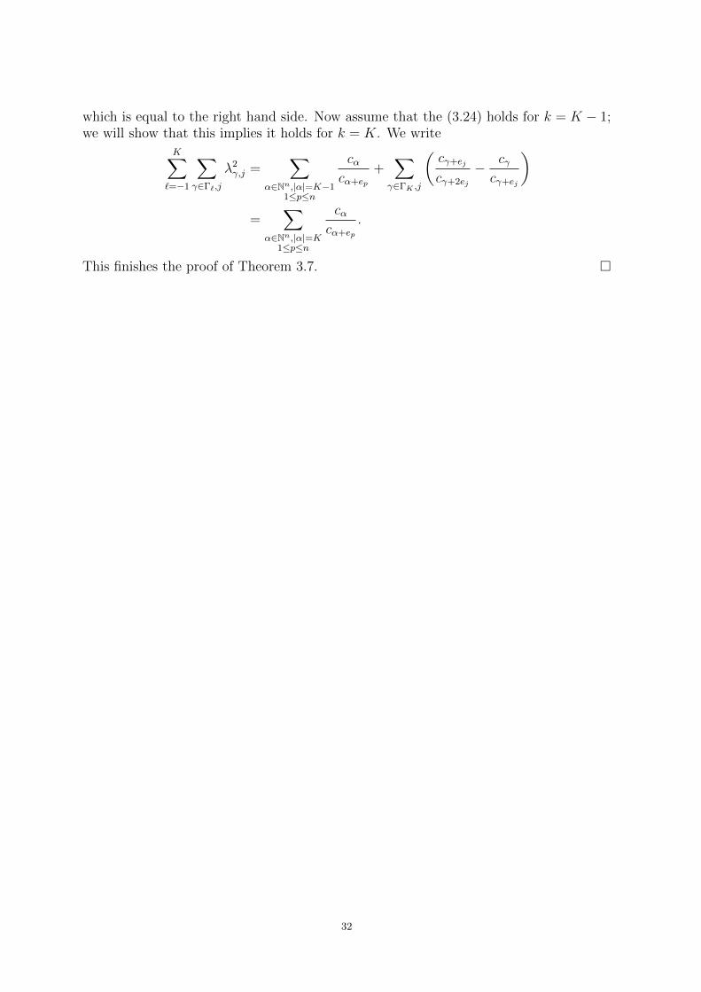
which is equal to the right hand side. Now assume that the (3.24) holds for k = K − 1;we will show that this implies it holds for k = K. We write

K∑`=−1

∑γ∈Γ`,j

λ2γ,j =

∑α∈Nn,|α|=K−1

1≤p≤n

cαcα+ep

+∑

γ∈ΓK ,j

(cγ+ej

cγ+2ej

− cγcγ+ej

)

=∑

α∈Nn,|α|=K1≤p≤n

cαcα+ep

.

This finishes the proof of Theorem 3.7.

32

4. The ∂-complex

Our main task will be to solve the inhomogeneous Cauchy-Riemann equation ∂u = f,where the right hand side f is given and satisfies the necessary condition ∂f = 0. Forn > 1 this is an overdetermined system of partial differential equations, which will bereduced to a system with equal numbers of unknowns and equations.We demonstrate this method first in its finite dimensional analog: let E,F,G denote finitedimensional vector spaces over C with inner product. We consider an exact sequence oflinear maps

ES−→ F

T−→ G,

which means that ImS = KerT, hence TS = 0.Given f ∈ ImS = KerT, we want to solve Su = f with u ⊥ KerS, then u will be calledthe canonical solution.For this purpose we investigate

ES−→←−S∗

FT−→←−T∗

G

and observe that KerT = (ImT ∗)⊥ and KerT ∗ = (ImT )⊥. We claim that the operator

SS∗ + T ∗T : F −→ F

is bijective. Let (SS∗ + T ∗T )g = 0, then SS∗g = −T ∗Tg, which implies

SS∗g ∈ ImT ∗ ∩ ImS = ImT ∗ ∩KerT = ImT ∗ ∩ (ImT ∗)⊥ = 0,

hence SS∗g = T ∗Tg = 0, but this gives S∗g ∈ KerS∩ImS∗ = KerS∩(KerS)⊥ = 0, andg ∈ KerS∗ = (ImS)⊥; from T ∗Tg = 0 we get Tg ∈ KerT ∗ ∩ ImT = (ImT )⊥ ∩ ImT = 0and g ∈ KerT = ImS, therefore we obtain g ∈ ImS ∩ (ImS)⊥ = 0. So SS∗ + T ∗T isinjective and as F is finite dimensional SS∗ + T ∗T is bijective.Let N = (SS∗ + T ∗T )−1. We claim that

u = S∗Nf

is the canonical solution to Su = f. So we have to show that SS∗Nf = f and S∗Nf ⊥KerS. The latter easily follows from the fact that S∗Nf ∈ ImS∗ = (KerS)⊥.We have

f = SS∗Nf + T ∗TNf,

therefore the assumption Tf = 0 implies

0 = Tf = TSS∗Nf + TT ∗TNf = TT ∗TNf,

since TS = 0. From here we obtain

0 = (TT ∗TNf, TNf) = (T ∗TNf, T ∗TNf)

and T ∗TNf = 0, hence SS∗Nf = f and we are done.

In the following we will use this method for the ∂-operator.

33

Let Ω = z ∈ Cn : r(z) < 0, where

∇zr := (∂r

∂z1

, . . . ,∂r

∂zn) 6= 0

on bΩ = z : r(z) = 0. Without loss of generality we can suppose that |∇zr| = |∇r| = 1on bΩ. For u, v ∈ C∞(Ω) and

(u, v) =

∫Ω

u(z)v(z) dλ(z)

we have

(uxk , v) = −(u, vxk) +

∫bΩ

u(z)v(z) rxk(z) dσ(z),

where dσ is the surface measure on bΩ.This follows from the Green-Gauß -theorem: for ω ⊆ Rn we have∫

ω

∇ . F (x) dλ(x) =

∫bω

(F (x), ν(x)) dσ(x),

where ν(x) = ∇r(x) is the normal to bω at x, and F is a C1 vector field on ω, and

∇ . F (x) =n∑j=1

∂Fj∂xj

.

For k = 1 and F = (uv, 0, . . . , 0) one gets

(ux1 , v) = −(u, vx1) +

∫bΩ

u(z)v(z) rx1(z) dσ(z),

similarly one obtains

(4.1)

(∂u

∂zk, v

)= −

(u,

∂v

∂zk

)+

∫bΩ

u(z) v(z)∂r

∂zk(z) dσ(z).

Definition 4.1. Let Ω be a bounded domain in Cn with n ≥ 2, and let r be a C2 definingfunction for Ω. The Hermitian form

(4.2) i∂∂r(t, t)(p) =n∑

j,k=1

∂2r

∂zj∂zk(p) tjtk, p ∈ bΩ,

defined for all t = (t1, . . . , tn) ∈ Cn with∑n

j=1 tj(∂r/∂zj)(p) = 0 is called the Levi formof the function r at the point p.

The Levi form associated with Ω is independent of the defining function up to a positivefactor.For p ∈ bΩ, let

T 1,0p (bΩ) = t = (t1, . . . , tn) ∈ Cn :

n∑j=1

tj(∂r/∂zj)(p) = 0.

Then T 1,0p (bΩ) is the space of type (1, 0) vector fields which are tangent to the boundary

at the point p.Analogously

T 0,1p (bΩ) = t = (t1, . . . , tn) ∈ Cn :

n∑j=1

tj(∂r/∂zj)(p) = 0,

34

smooth sections in T 0,1p (bΩ) are the tangential Cauchy-Riemann operators, for instance

∂r

∂zk

∂

∂zj− ∂r

∂zj

∂

∂zk,

where j 6= k.

Definition 4.2. Let Ω be a bounded domain in Cn with n ≥ 2, and let r be a C2 definingfunction for Ω. Ω is called (Levi) pseudoconvex at p ∈ bΩ, if the Levi form

i∂∂r(t, t)(p) =n∑

j,k=1

∂2r

∂zj∂zk(p) tjtk ≥ 0

for all t ∈ T 1,0p (bΩ). The domain Ω is said to be strictly pseudoconvex at p, if the Levi

form is strictly positive for all such t 6= 0. Ω is called a (Levi) pseudoconvex domain if Ωis (Levi) pseudoconvex at every boundary point of Ω.A C2 real valued function ϕ on Ω is plurisubharmonic, if

n∑j,k=1

∂2ϕ

∂zj∂zk(z) tjtk ≥ 0,

for all t = (t1, . . . , tn) ∈ Cn and all z ∈ Ω.

A bounded domain Ω in Cn with n ≥ 2 with C2 boundary is pseudoconvex if andonly if Ω has a smooth strictly plurisubharmonic exhaustion function ϕ, i.e. the setsz ∈ Ω : ϕ(z) < c are relatively compact in Ω, for every c ∈ R.

Definition 4.3. Let Ω ⊆ Cn be a domain.

L2(0,1)(Ω) := u =

n∑j=1

uj dzj : uj ∈ L2(Ω) j = 1, . . . , n

is the space of (0, 1)- forms with coefficients in L2, for u, v ∈ L2(0,1)(Ω) we define the

inner product by

(u, v) =n∑j=1

(uj, vj).

In this way L2(0,1)(Ω) becomes a Hilbert space. (0, 1) forms with compactly supported

C∞ coefficients are dense in L2(0,1)(Ω).

Definition 4.4. Let f ∈ C∞0 (Ω) and set

∂f :=n∑j=1

∂f

∂zjdzj,

then

∂ : C∞0 (Ω) −→ L2(0,1)(Ω).

∂ is a densely defined unbounded operator on L2(Ω). It does not have closed graph.

35

Definition 4.5. The domain dom(∂) of ∂ consists of all functions f ∈ L2(Ω) such that∂f, in the sense of distributions, belongs to L2

(0,1)(Ω), i.e. ∂f = g =∑n

j=1 gj dzj, and for

each φ ∈ C∞0 (Ω) we have

(4.3)

∫Ω

n∑j=1

f

(∂φ

∂zj

)−dλ = −

∫Ω

n∑j=1

gj φ dλ.

It is clear that C∞0 (Ω) ⊆ dom(∂), hence dom(∂) is dense in L2(Ω). Since differentiationis a continuous operation in distribution theory we have

Lemma 4.6. ∂ : dom(∂) −→ L2(0,1)(Ω) has closed graph and Ker∂ is a closed subspace

of L2(Ω).

Proof. Let (fk)k be a sequence in dom(∂) such that fk → f in L2(Ω) and ∂fk → g inL2

(0,1)(Ω). We have to show that ∂f = g. Let h ∈ C∞0,(0,1)(Ω). Then∫Ω

n∑j=1

∂f

∂zjhj dλ = −

∫Ω

n∑j=1

f

(∂hj∂zj

)−dλ

= − limk→∞

∫Ω

n∑j=1

fk

(∂hj∂zj

)−dλ = lim

k→∞

∫Ω

n∑j=1

∂fk∂zj

hj dλ =

∫Ω

n∑j=1

gj hj dλ,

which means that ∂f = g.Now we can apply Lemma 13.8 and get that Ker∂ is a closed subspace of L2(Ω).

Ker∂ coincides with the Bergman space A2(Ω) of all holomorphic functions on Ω belong-ing to L2(Ω). This is due to the fact that ∂f

∂zk= 0 in the sense of distributions, implies

that f is already a holomorphic function (regularity of the Cauchy-Riemann operator,see for instance [2]).More general for q ≥ 1 : ∂ : L2

(0,q)(Ω) −→ L2(0,q+1)(Ω) with domain as before, is again

a densely defined, closed operator. In this case Ker∂ is a closed subspace of L2(0,q)(Ω),

which does not mean that all coefficients are holomorphic functions. The (0, 1) formf(z1, z2) = z2 dz1 + z1 dz2 satisfies ∂f = 0, but has non-holomorphic coefficients.

Proposition 4.7. Let Ω be a smoothly bounded domain in Cn, with defining functionr such that |∇r(z)| = 1 on bΩ. We set C∞(Ω) for the restriction of C∞(Cn) to Ω and

D0,1 = C∞(0,1)(Ω) ∩ dom(∂∗). A (0, 1)-form u =

∑nj=1 uj dzj with coefficients in C∞(Ω)

belongs to D0,1 if and only if∑n

j=1∂r∂zj

uj = 0 on bΩ.

Proof. For ψ ∈ C∞(Ω) ⊂ dom(∂) we haven∑j=1

(−∂uj∂zj

, ψ

)=

n∑j=1

(uj,

∂ψ

∂zj

)−

n∑j=1

∫bΩ

ujψ∂r

∂zjdσ = (u, ∂ψ)−

n∑j=1

∫bΩ

ujψ∂r

∂zjdσ,

if ψ has in addition compact support in Ω, we have

(∂∗u, ψ) = (u, ∂ψ).

Since the compactly supported smooth function are dense in L2(Ω), we must haven∑j=1

∫bΩ

ujψ∂r

∂zjdσ = 0,

36

for any ψ ∈ C∞(Ω). This implies

n∑j=1

uj∂r

∂zj= 0

on bΩ.

Now we consider the ∂-complex

(4.4) L2(Ω)∂−→ L2

(0,1)(Ω)∂−→ . . .

∂−→ L2(0,n)(Ω)

∂−→ 0 ,

where L2(0,q)(Ω) denotes the space of (0, q)-forms on Ω with coefficients in L2(Ω). The

∂-operator on (0, q)-forms is given by

(4.5) ∂

(∑J

′aJ dzJ

)=

n∑j=1

∑J

′ ∂aJ∂zj

dzj ∧ dzJ ,

where∑′

means that the sum is only taken over strictly increasing multi-indices J.The derivatives are taken in the sense of distributions, and the domain of ∂ consistsof those (0, q)-forms for which the right hand side belongs to L2

(0,q+1)(Ω). So ∂ is a

densely defined closed operator, and therefore has an adjoint operator from L2(0,q+1)(Ω)

into L2(0,q)(Ω) denoted by ∂

∗.

We consider the ∂-complex

(4.6) L2(0,q−1)(Ω)

∂−→←−∂∗

L2(0,q)(Ω)

∂−→←−∂∗

L2(0,q+1)(Ω),

for 1 ≤ q ≤ n− 1.

We remark that a (0, q + 1)-form u =∑′

J uJ dzJ belongs to C∞(0,q+1)(Ω) ∩ dom(∂∗) if and

only if

(4.7)n∑k=1

ukK∂r

∂zk= 0

on bΩ for all K with |K| = q. To see this let α ∈ C∞(0,q)(Ω)

(u, ∂α) = (∑|J |=q+1

′uJ dzJ ,

n∑j=1

∑|K|=q

′ ∂αK∂zj

dzj ∧ dzK)

=n∑j=1

∑|K|=q

′∫

Ω

ujK∂αK∂zj

dλ

= −n∑j=1

∑|K|=q

′∫

Ω

∂ujK∂zj

αK dλ+n∑j=1

∑|K|=q

′∫bΩ

ujK αK∂r

∂zjdσ

= (∑|K|=q

′(−n∑j=1

∂ujK∂zj

) dzK ,∑|K|=q

′αK dzK) +∑|K|=q

′∫bΩ

(n∑j=1

ujK∂r

∂zj)αK dσ

= (ϑu, α)−∫bΩ

〈θ(ϑ, dr)u, α〉 dσ,

37

where

(4.8) ϑu =∑|K|=q

′(−n∑j=1

∂ujK∂zj

) dzK

and

(4.9)∑|K|=q

′∫bΩ

(n∑j=1

ujK∂r

∂zj)αK dσ = −

∫bΩ

〈θ(ϑ, ∂r)u, α〉 dσ,

hence we have

(4.10) (ϑu, α) = (u, ∂α) +

∫bΩ

〈θ(ϑ, ∂r)u, α〉 dσ,

where θ(ϑ, dr)u denotes the symbol of ϑ in the ∂r direction. Note that for u ∈ dom(∂∗)

we have ∂∗u = ϑu.

Similarly we have for u ∈ C∞(0,q)(Ω) and α ∈ C∞(0,q+1)(Ω):

(4.11) (∂u, α) = (u, ϑα) +

∫bΩ

〈∂r ∧ u, α〉 dσ,

where

(4.12)

∫bΩ

〈∂r ∧ u, α〉 dσ =∑|K|=q

′n∑k=1

∫bΩ

uK∂r

∂zkαkK dσ.

Proposition 4.8. The complex Laplacian 2 = ∂ ∂∗

+ ∂∗∂ defined on

dom(2) = u ∈ L2(0,q)(Ω) : u ∈ dom(∂) ∩ dom(∂

∗) , ∂u ∈ dom(∂

∗) and ∂

∗u ∈ dom(∂)

acts as an unbounded, densely defined, closed and self-adjoint operator on L2(0,q)(Ω), 1 ≤

q ≤ n, which means that 2 = 2∗ and dom(2) = dom(2∗).

Proof. dom(2) contains all smooth forms with compact support, hence 2 is densely

defined. To show that 2 is closed depends on the fact that both ∂ and ∂∗

are closed :note that

(4.13) (2u, u) = (∂ ∂∗u+ ∂

∗∂u, u) = ‖∂u‖2 + ‖∂∗u‖2,

for u ∈ dom(2). We have to prove that for every sequence uk ∈ dom(2) such thatuk → u in L2

(0,q)(Ω) and 2uk converges, we have u ∈ dom(2) and 2uk → 2u. It follows

from (4.13) that

(2(uk − u`), uk − u`) = ‖∂(uk − u`)‖2 + ‖∂∗(uk − u`)‖2,

which implies that ∂uk converges in L2(0,q+1)(Ω) and ∂

∗uk converges in L2

(0,q−1)(Ω). Since

∂ and ∂∗

are closed operators, we get u ∈ dom(∂)∩dom(∂∗) and ∂uk → ∂u in L2

(0,q+1)(Ω)

and ∂∗uk → ∂

∗u in L2

(0,q−1)(Ω).

To show that ∂u ∈ dom(∂∗) and ∂

∗u ∈ dom(∂), we first notice that ∂ ∂

∗uk and ∂

∗∂uk

are orthogonal which follows from

(∂ ∂∗uk, ∂

∗∂uk) = (∂

2∂∗uk, ∂uk) = 0.

38

Therefore the convergence of 2uk = ∂ ∂∗uk +∂

∗∂uk implies that both ∂ ∂

∗uk and ∂

∗∂uk

converge. Now use again that ∂ and ∂∗

are closed operators to obtain that ∂ ∂∗uk → ∂ ∂

∗u

and ∂∗∂uk → ∂

∗∂u. This implies that 2uk → 2u. Hence 2 is closed.

In order to show that 2 is self-adjoint we use Lemma 13.11 from the appendix. Define

R = ∂ ∂∗

+ ∂∗∂ + I

on dom(2). By Lemma 13.11 both (I+∂ ∂∗)−1 and (I+∂

∗∂)−1 are bounded, self-adjoint

operators. Consider

L = (I + ∂ ∂∗)−1 + (I + ∂

∗∂)−1 − I.

Then L is bounded and self-adjoint. We claim that L = R−1. Since

(I + ∂ ∂∗)−1 − I = (I − (I + ∂ ∂

∗))(I + ∂ ∂

∗)−1 = −∂ ∂∗(I + ∂ ∂

∗)−1,

we have that the range of (I + ∂ ∂∗)−1 is contained in dom(∂ ∂

∗). Similarly, we have that

the range of (I + ∂∗∂)−1 is contained in dom(∂

∗∂) and we get

L = (I + ∂∗∂)−1 − ∂ ∂∗(I + ∂ ∂

∗)−1.

Since ∂2

= 0, we have that the range of L is contained in dom(∂∗∂) and

∂∗∂L = ∂

∗∂(I + ∂

∗∂)−1.

Similarly, we have that the range of L is contained in dom(∂ ∂∗) and

∂ ∂∗L = ∂ ∂

∗(I + ∂ ∂

∗)−1.

This implies that the range of L is contained in dom(2). In addition we have

RL = ∂ ∂∗(I + ∂ ∂

∗)−1 + ∂

∗∂(I + ∂

∗∂)−1 + L = I.

If Ru = 0, we get 2u = −u and 0 ≤ (2u, u) = −(u, u), which implies that u = 0.Hence R is injective and we have that L = R−1. By Lemma 13.11 we know that L isself-adjoint. Apply Lemma 13.10 to get that R is self-adjoint. Therefore 2 = R − I isself-adjoint.

In the sequel we will show that for a smoothly bounded pseudoconvex domain Ω we have

(4.14) ‖∂u‖2 + ‖∂∗u‖2 ≥ c ‖u‖2,

for each u ∈ dom(∂)∩dom(∂∗), c > 0 (see Theorem 7.1 ). Since (2u, u) = ‖∂u‖2+‖∂∗u‖2,

it follows that for a convergent sequence (2un)n we get

‖2un −2um‖ ‖un − um‖ ≥ (2(un − um), un − um) ≥ c‖un − um‖2,

which implies that (un)n is convergent and since 2 is a closed operator we obtain that

2 has closed range. If 2u = 0, we get ∂u = 0 and ∂∗u = 0 and by (4.14) also that

u = 0, hence 2 is injective. By Lemma 13.10 (ii) the image of 2 is dense, therefore 2 issurjective.We showed that

2 : dom(2) −→ L2(0,q)(Ω)

is bijective and has a bounded inverse N : L2(0,q)(Ω) −→ dom(2). (Lemma 13.10 (iv) )

For u ∈ L2(0,q)(Ω) and v ∈ dom(∂) ∩ dom(∂

∗) we get

(4.15) (u, v) = (2Nu, v) = ((∂∂∗

+ ∂∗∂)Nu, v) = (∂

∗Nu, ∂

∗v) + (∂Nu, ∂v).

39

Let j : dom(∂)∩ dom(∂∗) −→ L2

(0,q)(Ω) denote the embedding, where dom(∂)∩ dom(∂∗)

is endowed with the graph-norm u 7→ (‖∂u‖2 + ‖∂∗u‖2)1/2, the graph-norm stems fromthe inner product

Q(u, v) = (u, v)Q = (2u, v) = (∂u, ∂v) + (∂∗u, ∂

∗v).

The basic estimates (4.14) imply that j is a bounded operator with operator norm

‖j‖ ≤ 1√c.

By (4.14) it follows in addition that dom(∂) ∩ dom(∂∗) endowed with the graph-norm

u 7→ (‖∂u‖2 + ‖∂∗u‖2)1/2 is a Hilbert space.Since (u, v) = (u, jv), we have that (u, v) = (j∗u, v)Q. Equation (4.15) suggests that as

an operator to dom(∂) ∩ dom(∂∗), N coincides with j∗ and as an operator to L2

(0,q)(Ω),

N should be equal to j j∗ (compare with Proposition 13.12). For this purpose setN = j j∗, and note that N∗ = (j j∗)∗ = j j∗ = N , i.e. N is self-adjoint (ofcourse also bounded). We claim that the range of N is contained in dom(2). To showthis we use an approach due to F. Berger (see [3]): since 2 is self-adjoint it suffices toshow that Nu ∈ dom(2∗) for all u ∈ L2

(0,q)(Ω), which means to show that the functional

v 7→ (2v, Nu) is bounded on dom(2) :

|(2v, Nu)| = |((∂ ∂∗ + ∂∗∂)v, Nu)| = |(∂v, ∂Nu) + (∂

∗v, ∂

∗Nu)|

= |(Q(v, j∗u)| = |(jv, u)| = |(v, u)| ≤ ‖v‖ ‖u‖.For v ∈ dom(∂) ∩ dom(∂

∗) we have

(2Nu, v) = (Nu, v)Q = (j∗u, v)Q = (u, jv) = (u, v),

hence 2Nu = u, in a similar way we obtain for u ∈ dom(2)

(N2u, v) = (2u, Nv) = (u, Nv)Q = (u, j∗v)Q = (ju, v) = (u, v),

which implies that N2u = u. Altogether we obtain that N = N .Now we get

‖∂Nu‖2 + ‖∂∗Nu‖2 = (j∗u, j∗u)Q ≤ ‖j∗‖2 ‖u‖2,

for u ∈ L2(0,q)(Ω), which implies that the operators

∂N : L2(0,q)(Ω) −→ L2

(0,q+1)(Ω) and ∂∗N : L2

(0,q)(Ω) −→ L2(0,q−1)(Ω)

are both bounded.Let Nq denote the ∂-Neumann operator on L2

(0,q)(Ω) and u ∈ dom(∂). Then ∂u =

∂∂∗∂Nqu and

Nq+1∂u = Nq+1∂ ∂∗∂Nqu = Nq+1(∂ ∂

∗+ ∂

∗∂)∂Nqu = ∂Nqu,

hence on dom(∂) we have

(4.16) Nq+1∂ = ∂Nq.

Similarly on dom(∂∗) we have

(4.17) Nq−1∂∗

= ∂∗Nq.

Since we already know that both operators ∂Nq and ∂∗Nq are bounded, we can continue

both operators Nq+1∂ and Nq−1∂∗

to bounded operators on L2(0,q)(Ω).

40

We remark that ∂∗Nq is zero on (ker(∂)⊥ : let k ∈ (ker∂)⊥ and u ∈ dom(∂), then

(∂∗Nqk, u) = (Nqk, ∂u) = (k,Nq∂u) = (k, ∂Nq−1u) = 0,

since ∂Nq−1u ∈ ker(∂), which gives ∂∗Nqk = 0.

For u ∈ L2(0,q)(Ω) we use (4.14) for Nqu to obtain

c‖Nqu‖2 ≤ ‖∂Nqu‖2+‖∂∗Nqu‖2 = (∂∗∂Nqu,Nqu)+(∂∂

∗Nqu,Nqu) = (u,Nqu) ≤ ‖u‖ ‖Nqu‖,

which implies

(4.18) ‖Nqu‖ ≤1

c‖u‖.

Given α ∈ L2(0,q)(Ω), with ∂α = 0 we get

(4.19) α = ∂ ∂∗Nqα + ∂

∗∂Nqα.

If we apply ∂ to the last equality we obtain:

0 = ∂α = ∂∂∗∂Nqα,

since ∂Nqα ∈ dom(∂∗) we have

0 = (∂ ∂∗∂Nqα, ∂Nqα) = (∂

∗∂Nqα, ∂

∗∂Nqα) = ‖∂∗∂Nqα‖2.

Finally we set u0 = ∂∗Nqα and derive from (4.19) that for ∂α = 0

α = ∂u0,

and we see that u0⊥ ker ∂, since for h ∈ ker ∂ we get

(u0, h) = (∂∗Nqα, h) = (Nqα, ∂h) = 0.

It follows that

‖∂∗Nqα‖2 = (∂ ∂∗Nqα,Nqα) = (∂ ∂

∗Nqα,Nqα)+(∂

∗∂Nqα,Nqα) = (α,Nqα) ≤ ‖α‖ ‖Nqα‖

and using (4.18) we obtain

(4.20) ‖∂∗Nqα‖ ≤ c−1/2 ‖α‖,

hence the canonical solution operator Sq for ∂ coincides with ∂∗Nq as operator on

L2(0,q)(Ω) ∩ ker∂

and is a bounded operator.Using (4.16) and (4.17) we now show that

(4.21) Nq = S∗q Sq + Sq+1 S∗q+1.

First note that by 13.3 we have

∂∗Nq = ∂

∗N∗q = (Nq∂)∗ and (∂

∗Nq)

∗ = Nq∂

and

∂Nq = ∂∗∗N∗q = (Nq∂

∗)∗ = (∂

∗Nq+1)∗ and ∂

∗Nq+1 = (∂Nq)

∗ = Nq∂∗,

41

hence it follows that for u ∈ L2(0,q)(Ω) we have

Nqu = Nq(∂ ∂∗

+ ∂∗∂)Nqu

= (Nq∂)(∂∗Nq)u+ (Nq∂

∗)(∂Nq)u

= (∂∗Nq)

∗(∂∗Nq)u+ (∂

∗Nq+1)(∂

∗Nq+1)∗u

= S∗q Squ+ Sq+1 S∗q+1u.

Let Pq : L2(0,q)(Ω) −→ ker∂ denote the orthogonal projection, which is the Bergman

projection for q = 0. We claim that

Pq = I − ∂∗Nq+1∂,

on dom(∂). First we show that the range of the right hand side, which we denote by P ,coincides with ker∂ : for u ∈ dom(∂) we have

∂u− ∂ ∂∗Nq+1∂u = ∂u−2Nq+1∂u+ ∂∗∂Nq+1∂u = ∂u− ∂u = 0,

where we used (4.16) to show that ∂Nq+1∂u = Nq+2∂ ∂u = 0, and since u−∂∗Nn+1∂u = u

for u ∈ ker∂, we have shown the first claim. Now we obtain

P ∗ = (I − ∂∗Nq+1∂)∗ = I − ∂∗Nq+1∂∗∗

= P ,

and

P 2u = P u− ∂∗Nq+1∂Pu

= P u− ∂∗Nq+1∂u+ ∂∗Nq+1∂ ∂

∗Nq+1∂u

= P u− ∂∗Nq+1∂u+ ∂∗Nq+1(2− ∂∗∂)Nq+1∂u

= P u.

This means that P coincides with Pq on dom(∂).

Finally we remark that P can be extended to a unique bounded operator on L2(0,q)(Ω),

with coincides with Pq : for u ∈ dom(∂) we have by (4.16) that ∂∗Nq+1∂u = ∂

∗∂Nqu and

u = 2Nqu = ∂ ∂∗Nqu+ ∂

∗∂Nqu is an orthogonal decomposition, which follows from

(∂ ∂∗Nqu, ∂

∗∂Nqu) = (∂ ∂ ∂

∗Nqu, ∂Nqu) = 0.

Hence

‖∂∗Nq+1∂u‖ = ‖∂∗∂Nqu‖ ≤ ‖u‖, u ∈ dom(∂),

which proves the claim since dom(∂) is dense in L2(0,q)(Ω).

Remark 4.9. If one supposes that

2 : dom(2) −→ L2(0,1)(Ω)

is bijective and has a bounded inverse N, the basic estimate (4.14) must hold; this followsfrom the spectral theorem, see [14]:N is self-adjoint and bounded and therefore has a bounded self-adjoint root N1/2 whichis again injective. By Lemma 13.10 N1/2 has a self-adjoint inverse which will be denotedby N−1/2. Let u ∈ dom(2). Then there exists w ∈ L2

(0,1)(Ω) such that Nw = u. Hence

42

we have N1/2v = u, where v = N1/2w and N−1/2v = w = N−1/2N−1/2u is well defined.Now we get

‖u‖2 = ‖N1/2v‖2 ≤ C‖v‖2 = C (N−1/2u,N−1/2u)

= C (N−1/2N−1/2u, u) = C (N−1/2N−1/2Nw,Nw)

= C (w,Nw) = C (2u, u)

≤ C (‖∂u‖2 + ‖∂∗u‖2),

which is the basic estimate (4.14).

The two boundary conditions u ∈ dom(∂∗) and ∂u ∈ dom(∂

∗) which appear in the

definition of dom(2) are called the ∂-Neumann boundary conditions. They amountto a Dirichlet boundary condition on the normal component of u and to the normalcomponent of ∂u respectively, see [46] for more details.

Example. Let Ω be a smoothly bounded domain in Cn with 0 ∈ bΩ. Assume that forsome neighborhood U of 0

Ω ∩ U = z ∈ Cn : =zn = yn < 0 ∩ U.

Let u =∑n

j=1 uj dzj ∈ C2(0,1)(Ω) and suppose that the support of u lies in U ∩ Ω. Then

u ∈ dom(2) if and only if

un = 0 on bΩ ∩ U,(4.22)

∂uj∂zn

= 0 on bΩ ∩ U, j = 1, . . . , n− 1.(4.23)

(4.22) follows from (4.7), which means that u ∈ dom(∂∗), and ∂u ∈ dom(∂

∗) is equivalent

to∂uj∂zn− ∂un∂zj

= 0 on bΩ ∩ U, j = 1, . . . , n− 1,

again by (4.7). Since ∂un∂zj

= 0 on bΩ ∩ U, j = 1, . . . , n− 1, we get (4.23).

It is the second boundary condition which makes the system non-coercive.

We continue investigating the boundary conditions:

Proposition 4.10. Let Ω be a smoothly bounded domain in Cn, with defining functionr such that |∇r(z)| = 1 on bΩ. Then, if u ∈ D0,1, we have

(4.24) ‖∂u‖2 + ‖∂∗u‖2 =n∑

j,k=1

∥∥∥∥∂uj∂zk

∥∥∥∥2

+

∫bΩ

n∑j,k=1

∂2r

∂zj∂zkuj uk dσ.

Proof. For u ∈ D0,1 we have

∂u =∑j<k

(∂uk∂zj− ∂uj∂zk

)dzj ∧ dzk,

and

∂∗u = −

n∑j=1

∂uj∂zj

.

43

For the norms we get

‖∂u‖2 =∑j<k

∥∥∥∥∂uk∂zj− ∂uj∂zk

∥∥∥∥2

=n∑

j,k=1

∥∥∥∥∂uk∂zj

∥∥∥∥2

−n∑

j,k=1

(∂uk∂zj

,∂uj∂zk

),

and

‖∂∗u‖2 =

∥∥∥∥∥n∑j=1

∂uj∂zj

∥∥∥∥∥2

=

(n∑j=1

∂uj∂zj

,n∑k=1

∂uk∂zk

).

Note that the commutator[

∂∂zk

, ∂∂zj

]= 0 and integrate by parts

−n∑

j,k=1

(∂uk∂zj

,∂uj∂zk

)=

n∑j,k=1

(∂

∂zk

∂uk∂zj

, uj

)−∫bΩ

∂r

∂zk

∂uk∂zj

uj dσ

=n∑

j,k=1

(∂

∂zj

∂uk∂zk

, uj

)−∫bΩ

∂r

∂zk

∂uk∂zj

uj dσ

=n∑

j,k=1

−(∂uk∂zk

,∂uj∂zj

)+

∫bΩ

∂r

∂zj

∂uk∂zk

uj dσ −∫bΩ

∂r

∂zk

∂uk∂zj

uj dσ

= −‖∂∗u‖2 +n∑

j,k=1

∫bΩ

∂r

∂zj

∂uk∂zk

uj dσ −n∑

j,k=1

∫bΩ

∂r

∂zk

∂uk∂zj

uj dσ.

Since u ∈ D0,1, which means that∑n

j=1∂r∂zj

uj = 0 on bΩ, the second term of the last line

is 0.Also since u ∈ D0,1, the vector field X :=

∑nk=1 uk

∂∂zk

is tangent to bΩ. Thus , if g is any

function vanishing on bΩ, then X(g) = 0 on bΩ. The function g0 =∑n

j=1∂r∂zj

uj = 0 on

bΩ. Hence we get

X(g0) =n∑k=1

uk∂

∂zk

(n∑j=1

∂r

∂zjuj

)=

n∑j,k=1

uk∂2r

∂zj∂zkuj +

n∑j,k=1

uk∂r

∂zj

∂uj∂zk

= 0.

Taking complex conjugates we see that

n∑j,k=1

∂r

∂zk

∂uk∂zj

uj = −n∑

j,k=1

∂2r

∂zj∂zkuj uk,

and since the right side is real this implies that

‖∂u‖2 =n∑

j,k=1

∥∥∥∥∂uk∂zj

∥∥∥∥2

− ‖∂∗u‖2 +

∫bΩ

n∑j,k=1

∂2r

∂zj∂zkuj uk dσ.

Corollary 4.11. Let Ω be a smoothly bounded pseudoconvex domain in Cn, with definingfunction r such that |∇r(z)| = 1 on bΩ. Then, if u ∈ D0,1, we have

(4.25) ‖∂u‖2 + ‖∂∗u‖2 ≥n∑

j,k=1

∥∥∥∥∂uj∂zk

∥∥∥∥2

.

44

Proof. By Definition 4.2 the Levi formn∑

j,k=1

∂2r

∂zj∂zk(p)uj(p)uk(p) ≥ 0,

for all p ∈ bΩ and for all u ∈ D0,1. Hence the result follows immediately from 4.10.

The following density result is crucial for the whole analysis.

Proposition 4.12. If bΩ is Ck+1, then Ck(0,q)(Ω)∩dom(∂∗) is dense in dom(∂)∩dom(∂

∗)

in the graph norm u 7→ (‖u‖2 + ‖∂u‖2 + ‖∂∗u‖2)1/2. The statement also holds with k+ 1and k replaced by ∞.

Before we begin with the proof of this important approximation result we mention a fewconsequences of it.

Remark 4.13. (a) From Proposition 4.12 it follows that D0,q is dense in dom(∂) ∩dom(∂

∗) in the graph norm u 7→ (‖u‖2 +‖∂u‖2 +‖∂∗u‖2)1/2. If (4.14) holds, we can take

u 7→ (‖∂u‖2 + ‖∂∗u‖2)1/2 instead of u 7→ (‖u‖2 + ‖∂u‖2 + ‖∂∗u‖2)1/2.

(b) It is also useful to know that dom(∂∗) is preserved under multiplication by a function

in C1(Ω) : let u ∈ dom(∂∗) , v ∈ dom(∂) and ψ ∈ C1(Ω). Then

(∂v, ψu) = (ψ ∂v, u) = (∂(ψv), u)− (∂ ψ ∧ v, u) = (ψv, ∂∗u)− (∂ ψ ∧ v, u).

The right-hand side is bounded by ‖v‖, hence ψu ∈ dom(∂∗), (see [46] for more details).

(c) Compactly supported forms are not dense in dom(∂) ∩ dom(∂∗) in the graph norm:

for compactly supported forms Proposition 4.10 gives

‖∂u‖2 + ‖∂∗u‖2 =n∑

j,k=1

∥∥∥∥∂uj∂zk

∥∥∥∥2

,

and integration by parts also shows that in this case∥∥∥∥∂uj∂zk

∥∥∥∥2

=

∥∥∥∥∂uj∂zk

∥∥∥∥2

.

Hence‖u‖2

1 ≤ 2 (‖∂u‖2 + ‖∂∗u‖2),

where ‖u‖21 denotes the standard Sobolev-1 norm of u on Ω. Therefore the closure of the

compactly supported forms in dom(∂) ∩ dom(∂∗) in the graph norm is contained in the

Sobolev space W 10 (Ω) for forms that are C∞ on Ω, this means that they are zero on the

boundary, which is stronger than the conditionn∑j=1

∂r

∂zjuj = 0

on bΩ from Proposition 4.7.

(d) If Ω is a smoothly bounded pseudoconvex domain, then dom(∂)∩dom(∂∗) is a Hilbert

space in the graph norm u 7→ (‖∂u‖2 + ‖∂∗u‖2)1/2. This follows from (4.14).

We follow the reasoning in [9] to prove Proposition 4.12.

45

Lemma 4.14. Let Ω be as in Proposition 4.12. Then C∞(0,q)(Ω) is dense in dom(∂) ∩dom(∂

∗) in the graph norm u 7→ (‖u‖2 + ‖∂u‖2 + ‖∂∗u‖2)1/2.

Proof. By this we mean that if u ∈ dom(∂) ∩ dom(∂∗), one can construct a sequence

um ∈ C∞(0,q)(Ω) such that um → u , ∂um → ∂f and ϑum → ϑu in L2(Ω).We use a method closely related to Friedrichs’ Lemma 16.3 and use the notation fromthere.Let (χε)ε be an approximation of the identity and (δν)ν a sequence of small positivenumbers with δν → 0, and define

Ωδν = z ∈ Ω : r(z) < −δν.Then Ωδν is a sequence of relatively compact open subsets of Ω with union equal to Ω.The forms uε = u ∗ χε belong to C∞(0,q)(Ωδν ) and uε → u , ∂uε → ∂u and ϑuε → ϑu in

L2(Ωδν ), see Lemma 16.2 and Lemma 16.3.To see that this can be done up to the boundary, we first assume that the domain Ω isstar-shaped and 0 ∈ Ω is a center. Let Ωε = (1 + ε)z : z ∈ Ω and

uε(z) = u

(z

1 + ε

),

where the dilation is performed for each coefficient of u. Then Ω ⊂⊂ Ωε and uε ∈ L2(Ωε).Also, by the dominated convergence theorem, uε → u , ∂uε → ∂u and ϑuε → ϑu inL2(Ω). Now we regularize uε defining

(4.26) u(ε) = uε ∗ χδε ,

where δε → 0 as ε → 0 and δε is chosen sufficiently small. Then u(ε) ∈ C∞(0,q)(Ω) and

u(ε) → u , ∂u(ε) → ∂u and ϑu(ε) → ϑu in L2(Ω). Thus, C∞(0,q)(Ω) is dense in the graphnorm when Ω is star-shaped. The general case follows by using a partition of unity sincewe assume that our domain has at least C2 boundary.

Lemma 4.15. Let Ω be as in Proposition 4.12. Then compactly supported smooth formsare dense in dom(∂

∗) in the graph norm u 7→ (‖u‖2 + ‖∂∗u‖2)1/2.

Proof. We remark that if u ∈ dom(∂∗) and if we extend u to u on the whole space Cn

by setting u to be zero outside of Ω, then ϑu ∈ L2(Cn) in the distribution sense: in fact

for u ∈ dom(∂∗) we have

ϑu = ϑu

where ϑu = ϑu in Ω and ϑu = 0 outside of Ω. This can be checked from the definitionof ∂

∗, since for any v ∈ C∞(0,q−1)(Cn),

(u, ∂v)L2(Cn) = (u, ∂v)L2(Ω) = (ϑu, v)L2(Ω) = (ϑu, v)L2(Cn).

We assume again without loss of generality that Ω is star-shaped with 0 as a center. Wefirst approximate u by

u−ε(z) = u

(z

1− ε

).

Now we have forms u−ε with compact support in Ω and ϑu−ε → ϑu in L2(Cn). Regular-izing u−ε as before, we define

(4.27) u(−ε) = u−ε ∗ χδε .

46

Then the u(−ε) are (0, q)-forms with coefficients in C∞0 (Ω) such that u(−ε) → u andϑu(−ε) → ϑu in L2(Ω).

However, compactly supported smooth forms are not dense in dom(∂) in the graph normu 7→ (‖u‖2 + ‖∂u‖2)1/2. Nevertheless, we have

Lemma 4.16. Let Ω be as in Proposition 4.12. Then Ck(0,q)(Ω) ∩ dom(∂∗) is dense in

dom(∂) in the graph norm u 7→ (‖u‖2 + ‖∂u‖2)1/2.

Proof. By Lemma 4.14 it suffices to show that for any u ∈ C∞(0,q)(Ω) one can find a

sequence um ∈ Ck(0,q)(Ω) ∩ dom(∂∗) such that um → u and ∂um → ∂u in L2(Ω).

Let r be a Ck+1 defining function such that |dr| = 1 on bΩ. We now introduce somespecial vector fields and (1, 0)-forms associated with bΩ. Near a point p ∈ bΩ we choosefields L1, L2, . . . , Ln−1 of type (1, 0) that are orthonormal and span T 1,0

p (bΩ). This can bedone by choosing a basis, and then using the Gram-Schmidt process. To this collectionadd Ln, the complex normal, normalized to have length 1. So Ln is a smooth multiple of

n∑j=1

∂r

∂zj

∂

∂zj.

Now denote by w1, w2, . . . w2 the (1, 0)-forms such that wj(Lk) = δjk. Ln is definedglobally, in contrast to L1, . . . , Ln−1. The wj ’s then form an orthonormal basis for the(1, 0)-forms near p. The (1, 0)-form wn is a smooth multiple of

∑nj=1

∂r∂zj

dzj, and is again

globally defined. Taking wedge products of the wj’s yields (local) orthonormal bases forthe (1, 0)-forms.We will regularize near a boundary point p ∈ bΩ. Let U be a small neighborhood of p. By apartition of unity, we may assume that Ω∩U is star-shaped and u is supported in U ∩Ω.Shrinking U if necessary, we can choose a special boundary chart (t1, t2, . . . , t2n−1, r),where (t1, t2, . . . , t2n−1, 0) are coordinates on bΩ near p. Let w1, . . . , wn be an orthonormalbasis for the (0, 1)-forms on U such that ∂r = wn.Let Lj =

∑ns=1 ajs

∂∂zs

, wj =∑n

s=1 bjsdzs, 1 ≤ j ≤ n. Then

δjk = wj(Lk) =n∑s=1

bjs dzs (n∑`=1

ak`∂

∂z`) =

n∑s=1

bjsaks.

Consequently, if f is a function,

(4.28) ∂f =n∑s=1

∂f

∂zsdzs =

n∑j,k,s=1

ask(Lkf) bsj wj =n∑j=1

(Ljf)wj,

where the superscripts denote the entries of the inverses of the corresponding matriceswith subscripts. Since multiplication by functions in C1(Ω) preserves dom(∂

∗), we may

assume that the form u is supported in a special boundary chart. So u =∑|J |=q

′uJwJ ,

where wJ = wj1 ∧ · · · ∧ wjq and each uJ is a function in Ck(Ω). Then, in view of (4.28)

∂u = ∂(∑|J |=q

′uJwJ) =∑|J |=q

′(∂uJ ∧ wJ + uJ∂wJ)(4.29)

=∑|J |=q

′n∑j=1

(LjuJ)wj ∧ wJ +∑|J |=q

′uJ∂wJ .(4.30)

47

Using the special boundary chart we get from (4.7) that

(4.31) u ∈ dom(∂∗)⇐⇒ uJ = 0 on bΩ when n ∈ J.

Indeed, the only boundary terms that arise when proving (4.7) come from integrating∫Ω

LnαK unK dλ

by parts and they equal ∫bΩ

αK unK(Lnr) dσ.

Since αK can be arbitrary on bΩ and Lnr 6= 0 on bΩ, we conclude that unK = 0 on bΩ forall K. To see that the condition is sufficient, note that the computation to prove (4.10)shows that (u, ∂α) = (ϑu, α) when (4.7) holds and α ∈ C∞(0,q)(Ω). In view of Lemma

4.14 C∞(0,q)(Ω) is dense in dom(∂) in the graph norm u 7→ (‖u‖2 + ‖∂u‖2)1/2. Hence,

(u, ∂α) = (ϑu, α) for all α ∈ dom(∂), which implies u ∈ dom(∂∗) and ∂

∗u = ϑu.

These arguments also give a formula for ϑ and ∂∗

in special boundary frames:

(4.32) ϑu = ϑ(∑|J |=q

′uJwJ) = −∑|K|=q−1

′ (n∑j=1

LjujK)wK + 0-th order(u).

0-th order(u) indicates terms that contain no derivatives of the uJ ’s.

We note that both ∂ and ϑ are first order differential operators with variable coefficientsin Ck(Ω) when computed in the special frame w1, . . . , wn. We write

u = uτ + uν ,

whereuτ =

∑|J |=q,n/∈J

′ uJwJ , uν =

∑|J |=q,n∈J

′ uJwJ .

uτ is the complex tangential part of u, and uν is the complex normal part of u.Our arguments from above imply that

u ∈ Ck(0,q)(Ω) ∩ dom(∂∗) ⇐⇒ uν = 0 on bΩ.

For u ∈ C∞(0,q)(Ω) and α ∈ C∞(0,q+1)(Ω) we have by (4.11)

(∂u, α) = (u, ϑα) +

∫bΩ

〈∂r ∧ u, α〉 dσ

and ∂r ∧ u = ∂r ∧ uτ on bΩ, which follows from the representation in special boundarycharts:

(4.33) ∂r ∧ uν = cwn ∧∑

|J |=q,n∈J

′ uJwJ = 0.

In order to approximate a form u ∈ C∞(0,q)(Ω) by forms in Ck(0,q)(Ω) ∩ dom(∂∗) we only

change the complex normal part uν and leave the complex tangential part uτ unchanged:for u ∈ C∞(0,q)(Ω) it follows that uτ ∈ Ck(0,q)(Ω)∩dom(∂

∗) and we denote by uν the extension

of uν to Cn by setting uν equal to zero outside of Ω. We approximate uν as in Lemma4.15 by

uν(−ε) = (uν)−ε ∗ χδε .

48

Then uν(−ε) is smooth and supported in a compact subset of Ω∩U. By this, we approximate

uν by uν(−ε) ∈ C∞0 (Ω ∩ U) in the L2-norm. Furthermore, by extending ∂uν to be zero

outside Ω ∩ U and denoting the extension by ∂uν , we have

∂uν = ∂uν

in L2(Cn) in the sense of distributions. This follows from (4.11) and (4.33), since uν ∈Ck(0,q)(Ω) and for α ∈ C∞(0,q+1)(Cn) we have

(uν , ϑα)L2(Cn) = (∂uν , α)L2(Ω) −∫bΩ

〈∂r ∧ uν , α〉 dσ = (∂uν , α)L2(Cn).

Since ∂ is a first order differential operator with variable coefficients, we get fromFriedrichs’ Lemma 16.4

(4.34) ∂uν(−ε) → ∂uν in L2(Cn).

We set

u(−ε) = uτ + uν(−ε).

It follows that u(−ε) ∈ Ck(0,q)(Ω) ∩ dom(∂∗), since each coefficient of uτ , uν(−ε) and wj is in

Ck(Ω ∩ U). Therefore we get u(−ε) ∈ Ck(0,q)(Ω) ∩ dom(∂∗) and u(−ε) → u in L2(Ω).

To see that ∂u(−ε) → ∂u in the L2(Ω)-norm, using (4.34), we find that

∂u(−ε) = ∂uτ + ∂uν(−ε) → ∂u

in L2(Ω) as ε→ 0.

To finish the proof of Proposition 4.12 we consider an arbitrary u ∈ dom(∂) ∩ dom(∂∗)

and use a partition of unity and the same notation as before to regularize u in each smallstar-shaped neighborhood near the boundary. We regularize the complex tangential andnormal part separately by setting

u((ε)) = uτ(ε) + uν(−ε),

this means that we first consider u(ε) as it was defined in (4.26) and take then thetangential components uτ(ε), then we consider u(−ε) as it is defined in (4.27) and thentake the normal components uν(−ε). It follows that for sufficiently small ε > 0, uν(−ε) has

coefficients in C∞0 (Ω) and uτ(ε) has coefficients in C∞(Ω).

Thus we see that u((ε)) ∈ Ck(0,q)(Ω) ∩ dom(∂∗). We get from Lemma 4.14 that u(ε) → u in

the graph norm u 7→ (‖u‖2 +‖∂u‖2 +‖∂∗u‖2)1/2, hence uτ(ε) → uτ in the graph norm u 7→(‖u‖2+‖∂u‖2+‖∂∗u‖2)1/2. From Lemma 4.15 we obtain u(−ε) → u in the graph norm u 7→(‖u‖2 +‖∂∗u‖2)1/2, hence uν(−ε) → uν in the graph norm u 7→ (‖u‖2 +‖∂∗u‖2)1/2. Finally,

we use Lemma 4.16, in particular formula (4.34), and see that ∂uν(−ε) → ∂uν in L2(Cn),

hence u((ε)) → u in the graph norm u 7→ (‖u‖2 + ‖∂u‖2 + ‖∂∗u‖2)1/2.

This shows that Ck(0,q)(Ω) ∩ dom(∂∗) is dense in dom(∂) ∩ dom(∂

∗) in the graph norm

u 7→ (‖u‖2 + ‖∂u‖2 + ‖∂∗u‖2)1/2.

49

5. The weighted ∂-complex

Let ϕ : Cn −→ R+ be a plurisubharmonic C2-weight function and define the space

L2(Cn, e−ϕ) = f : Cn −→ C :

∫Cn|f |2 e−ϕ dλ <∞,

where λ denotes the Lebesgue measure, the space L2(0,1)(Cn, e−ϕ) of (0, 1)-forms with

coefficients in L2(Cn, e−ϕ) and the space L2(0,2)(Cn, e−ϕ) of (0, 2)-forms with coefficients

in L2(Cn, e−ϕ). Let

(f, g)ϕ =

∫Cnf ge−ϕ dλ

denote the inner product and

‖f‖2ϕ =

∫Cn|f |2e−ϕ dλ

the norm in L2(Cn, e−ϕ).We consider the weighted ∂-complex

(5.1) L2(Cn, e−ϕ)∂−→←−∂∗ϕ

L2(0,1)(Cn, e−ϕ)J

∂−→←−∂∗ϕ

L2(0,2)(Cn, e−ϕ),

where ∂∗ϕ is the adjoint operator to ∂ with respect to the weighted inner product. For

u =∑n

j=1 ujdzj ∈ dom(∂∗ϕ) one has

(5.2) ∂∗ϕu = −

n∑j=1

(∂

∂zj− ∂ϕ

∂zj

)uj.

The complex Laplacian on (0, 1)-forms is defined as

ϕ := ∂ ∂∗ϕ + ∂

∗ϕ∂,

where the symbol ϕ is to be understood as the maximal closure of the operator initiallydefined on forms with coefficients in C∞0 , i.e., the space of smooth functions with compactsupport.ϕ is a selfadjoint and positive operator, which means that

(ϕf, f)ϕ ≥ 0 , for f ∈ dom(ϕ).

The associated Dirichlet form is denoted by

(5.3) Qϕ(f, g) = (∂f, ∂g)ϕ + (∂∗ϕf, ∂

∗ϕg)ϕ,

for f, g ∈ dom(∂)∩ dom(∂∗ϕ). The weighted ∂-Neumann operator Nϕ is - if it exists - the

bounded inverse of ϕ. For further details see [22].

There is an interesting connection between ∂ and the theory of Schrodinger operatorswith magnetic fields, see for example [10], [4], [19] and [11] for recent contributionsexploiting this point of view.In the weighted space L2

(0,1)(Cn, e−ϕ) we can give a simple characterization of dom (∂∗ϕ)

(see [20]):

50

Proposition 5.1. Let f =∑fjdzj ∈ L2

(0,1)(Cn, e−ϕ). Then f ∈ dom(∂∗ϕ) if and only if

(5.4) eϕn∑j=1

∂

∂zj

(fje−ϕ) ∈ L2(Cn, e−ϕ),

where the derivative is to be taken in the sense of distributions.

Proof. Suppose first that eϕ∑n

j=1∂∂zj

(fje−ϕ) ∈ L2(Cn, e−ϕ). We have to show that there

exists a constant C such that |(∂g, f)ϕ| ≤ C‖g‖ϕ for all g ∈ dom(∂). To this end let(χR)R∈N be a family of radially symmetric smooth cutoff funtions, which are identicallyone on BR, the ball with radius R, such that the support of χR is contained in BR+1,supp(χR) ⊂ BR+1, and such that furthermore all first order derivatives of all functionsin this family are uniformly bounded by a constant M . Then for all g ∈ C∞0 (Cn):

(∂g, χRf)ϕ =n∑j=1

(∂g

∂zj, χRfj)ϕ = −

∫Cn

n∑j=1

g∂

∂zj

(χRf je

−ϕ) dλ,by integration by parts, which in particular means

|(∂g, f)ϕ| = limR→∞

|(∂g, χRf)ϕ| = limR→∞

∣∣∣∣∣∫Cn

n∑j=1

g∂

∂zj

(χRf je

−ϕ) dλ∣∣∣∣∣ .Now we use the triangle inequality, afterwards Cauchy – Schwarz, to get∣∣∣∣∣

∫Cn

n∑j=1

g∂

∂zj

(χRf je

−ϕ) dλ∣∣∣∣∣≤

∣∣∣∣∣∫CnχR g

n∑j=1

∂

∂zj

(f je−ϕ) dλ∣∣∣∣∣+

∣∣∣∣∣∫Cn

n∑j=1

f jg∂χR∂zj

e−ϕ dλ

∣∣∣∣∣≤‖χR g‖ϕ

∥∥∥∥∥eϕn∑j=1

∂

∂zj

(fje−ϕ)∥∥∥∥∥

ϕ

+M‖g‖ϕ‖f‖ϕ

=‖g‖ϕ

∥∥∥∥∥eϕn∑j=1

∂

∂zj

(fje−ϕ)∥∥∥∥∥

ϕ

+M‖g‖ϕ‖f‖ϕ.

Hence by assumption,

|(∂g, f)ϕ| ≤ ‖g‖ϕ

∥∥∥∥∥eϕn∑j=1

∂

∂zj

(fje−ϕ)∥∥∥∥∥

ϕ

+M‖g‖ϕ‖f‖ϕ ≤ C‖g‖ϕ

for all g ∈ C∞0 (Cn), and by density of C∞0 (Cn) this is true for all g ∈ dom(∂).

Conversely, let f ∈ dom(∂∗ϕ), which means that there exists a uniquely determined

element ∂∗ϕf ∈ L2(Cn, e−ϕ) such that for each g ∈ dom(∂) we have

(∂g, f)ϕ = (g, ∂∗ϕf)ϕ.

51

Now take g ∈ C∞0 (Cn). Then g ∈ dom(∂) and

(g, ∂∗ϕf)ϕ =(∂g, f)ϕ

=n∑j=1

(∂g

∂zj, fj)ϕ

=− (g,n∑j=1

∂

∂zj

(fje−ϕ))L2

=− (g, eϕn∑j=1

∂

∂zj

(fje−ϕ))ϕ.

Since C∞0 (Cn) is dense in L2(Cn, e−ϕ), we conclude that

∂∗ϕf = −eϕ

n∑j=1

∂

∂zj

(fje−ϕ) ,

which in particular implies that eϕ∑n

j=1∂∂zj

(fje−ϕ) ∈ L2(Cn, e−ϕ).

The following lemma will be important for our considerations.

Lemma 5.2. Forms with coefficients in C∞0 (Cn) are dense in dom(∂) ∩ dom(∂∗ϕ) in the

graph norm f 7→ (‖f‖2ϕ + ‖∂f‖2

ϕ + ‖∂∗ϕf‖2ϕ)

12 .

Proof. First we show that compactly supported L2-forms are dense in the graph norm.So let χRR∈N be a family of smooth radially symmetric cutoffs identically one on BRand supported in BR+1, such that all first order derivatives of the functions in this familyare uniformly bounded in R by a constant M .Let f ∈ dom(∂) ∩ dom(∂

∗ϕ). Then, clearly, χRf ∈ dom(∂) ∩ dom(∂

∗ϕ) and χRf → f in

L2(0,1)(Cn, e−ϕ) as R→∞. As observed in Proposition 5.1, we have

∂∗ϕf = −eϕ

n∑j=1

∂

∂zj

(fje−ϕ) ,

hence

∂∗ϕ(χRf) = −eϕ

n∑j=1

∂

∂zj

(χRfje

−ϕ) .We need to estimate the difference of these expressions

∂∗ϕf − ∂

∗ϕ(χRf) = ∂

∗ϕf − χR∂

∗ϕf +

n∑j=1

∂χR∂zj

fj,

which is by the triangle inequality

‖∂∗ϕf − ∂∗ϕ(χRf)‖ϕ ≤‖∂

∗ϕf − χR∂

∗ϕf‖ϕ +M

n∑j=1

∫Cn\BR

|fj|2e−ϕ dλ.

Now both terms tend to 0 as R→∞, and one can see similarly that also ∂(χRf)→ ∂fas R→∞.So we have density of compactly supported forms in the graph norm, and density of formswith coefficients in C∞0 (Cn) will follow by applying Friedrichs’ lemma, see 16.4.

52

As in the case of bounded domains, the canonical solution operator to ∂, which we denoteby Sϕ, is given by ∂

∗ϕNϕ. Existence and compactness of Nϕ and Sϕ are closely related.

Remark 5.3. In order to prove a basic estimate for the weighted ∂-complex we nowassume that the lowest eigenvalue µϕ of the Levi matrix

Mϕ =

(∂2ϕ

∂zj∂zk

)jk

satisfies

(5.3) µϕ(z) > ε, for all z ∈ Cn,

for some ε > 0.Using methods from real analysis, one can replace (6.5) by the the weaker assumptionthat

(5.3) lim inf|z|→∞

µϕ(z) > 0.

For this purpose we follow the reasoning in [26]. First we notice that

e−ϕ/2 2ϕ eϕ/2 = 4(0,1)

ϕ ,

where 4(0,1)ϕ is the Witten-Laplcian. Condition (5.3’) implies that 4(0,1)

ϕ is injective and

that the bottom of the essential spectrum σe(4(0,1)ϕ ) is positive (Persson’s Theorem). By

the spectral theorem for unbounded self-adjoint operators, one derives that 4(0,1)ϕ has a

bounded inverse, hence 2ϕ has a bounded inverse Nϕ and so the square root N1/2ϕ is also

bounded, which gives the basic estimate for the weighted ∂-complex .

Proposition 5.4.For a plurisubharmonic weight function ϕ satisfying (??), there is a C > 0 such that

(5.5) ‖u‖2ϕ ≤ C(‖∂u‖2

ϕ + ‖∂∗ϕu‖2ϕ)

for each (0, 1)-form u ∈dom (∂)∩ dom (∂∗ϕ).

Proof. By Lemma 5.2 and the assumption on ϕ it suffices to show that

(5.6)

∫Cn

n∑j,k=1

∂2ϕ

∂zj∂zkujuk e

−ϕ dλ ≤ ‖∂u‖2ϕ + ‖∂∗ϕu‖2

ϕ,

for each (0, 1)-form u =∑n

k=1 uk dzk with coefficients uk ∈ C∞0 (Cn), for k = 1, . . . , n.

For this purpose we set δk = ∂∂zk− ∂ϕ

∂zkand get since

∂u =∑j<k

(∂uj∂zk− ∂uk∂zj

)dzj ∧ dzk

that

‖∂u‖2ϕ + ‖∂∗ϕu‖2

ϕ =

∫Cn

∑j<k

∣∣∣∣∂uj∂zk− ∂uk∂zj

∣∣∣∣2 e−ϕ dλ+

∫Cn

n∑j,k=1

δjuj δkuk e−ϕ dλ

=n∑

j,k=1

∫Cn

∣∣∣∣∂uj∂zk

∣∣∣∣2 e−ϕ dλ+n∑

j,k=1

∫Cn

(δjuj δkuk −

∂uj∂zk

∂uk∂zj

)e−ϕ dλ

53

=n∑

j,k=1

∫Cn

∣∣∣∣∂uj∂zk

∣∣∣∣2 e−ϕ dλ+n∑

j,k=1

∫Cn

[δj,

∂

∂zk

]uj uk e

−ϕ dλ,

where we used the fact that for f, g ∈ C∞0 (Cn) we have(∂f

∂zk, g

)ϕ

= −(f, δkg)ϕ

and hence ([δj,

∂

∂zk

]uj, uk

)ϕ

= −(∂uj∂zk

,∂uk∂zj

)ϕ

+ (δjuj, δkuk)ϕ.

Since [δj,

∂

∂zk

]=

∂2ϕ

∂zj∂zk,

we have

(5.7) ‖∂u‖2ϕ + ‖∂∗ϕu‖2

ϕ =n∑

j,k=1

∫Cn

∣∣∣∣∂uj∂zk

∣∣∣∣2 e−ϕ dλ+n∑

j,k=1

∫Cn

∂2ϕ

∂zj∂zkujuk e

−ϕ dλ

and since ϕ satisfies (??) we are done (see also [30]).

At this stage we first generalize formula (5.7) for (0, q)-forms u =∑′|J |=q uJ dzJ with

coefficients in C∞0 (Cn). We notice that

∂u =∑|J |=q

′n∑j=1

∂uJ∂zj

dzj ∧ dzJ ,

and

∂∗ϕu = −

∑|K|=q−1

′n∑k=1

δkukK dzK .

We obtain

‖∂u‖2ϕ + ‖∂∗ϕu‖2

ϕ =∑

|J |=|M |=q

′n∑

j,k=1

εkMjJ

∫Cn

∂uJ∂zj

∂uM∂zk

e−ϕ dλ

+∑|K|=q−1

′n∑

j,k=1

∫Cn

δjujKδkukK e−ϕ dλ,

where εkMjJ = 0 if j ∈ J or k ∈ M or if k ∪ M 6= j ∪ J, and equals the sign of the

permutation(kMjJ

)otherwise. The right-hand side of the last formula can be rewritten as

(5.8)∑|J |=q

′n∑j=1

∥∥∥∥∂uJ∂zj

∥∥∥∥2

ϕ

+∑|K|=q−1

′n∑

j,k=1

∫Cn

(δjujKδkukK −

∂ujK∂zk

∂ukK∂zj

)e−ϕ dλ,

see [46] Proposition 2.4. Consider first the (nonzero) terms where j = k (and henceM = J). These terms result in the portion of the first sum in (5.8) where j /∈ J. Onthe other hand, when j 6= k, then j ∈ M and k ∈ J, and deletion of j from M and kfrom J results in the strictly increasing multi-index K of length q − 1. Consequently,these terms can be collected into the second sum in (5.8) ( the part with the minus sign,we have interchanged the summation indices j and k). In this sum, the terms where

54

j = k compensate for the terms in the first sum where j ∈ J. Now one can use the samereasoning as in the last proof to get

(5.9) ‖∂u‖2ϕ + ‖∂∗ϕu‖2

ϕ =∑|J |=q

′n∑j=1

∥∥∥∥∂uJ∂zj

∥∥∥∥2

ϕ

+∑|K|=q−1

′n∑

j,k=1

∫Cn

∂2ϕ

∂zj∂zkujKukK e

−ϕ dλ.

Proposition 5.5. For a plurisubharmonic weight function ϕ satisfying (??), there existsa uniquely determined bounded linear operator

Nϕ : L2(0,1)(Cn, e−ϕ) −→ L2

(0,1)(Cn, e−ϕ),

such that ϕ Nϕu = u, for any u ∈ L2(0,1)(Cn, ϕ). If u ∈ L2

(0,1)(Cn, ϕ) satisfies ∂u = 0,

then ∂∗ϕNϕu is the canonical solution of ∂f = u, which means that ∂

∗ϕNϕu⊥A2(Cn, ϕ),

where

A2(Cn, e−ϕ) = f : Cn −→ C entire : f ∈ L2(0,1)(Cn, e−ϕ).

Proof. First we mention that ϕ is a self-adjoint operator, which is proved in a similarway as in the case without weight in Chapter 4.For a given v ∈ L2

(0,1)(Cn, ϕ) consider the linear functional L on dom (∂)∩ dom (∂∗ϕ)

given by L(u) = (u, v)ϕ. Notice that dom (∂)∩ dom (∂∗ϕ) is a Hilbert space with the

inner product Qϕ. Since we have by Proposition 5.4

|L(u)| = |(u, v)ϕ| ≤ ‖u‖ϕ ‖v‖ϕ ≤ CQϕ(u, u)1/2 ‖v‖ϕ.Hence by the Riesz representation theorem there exists a uniquely determined (0, 1)-form

Nϕv ∈ dom(∂) ∩ dom(∂∗ϕ) such that

(u, v)ϕ = Qϕ(u,Nϕv) = (∂u, ∂Nϕv)ϕ + (∂∗ϕu, ∂

∗ϕNϕv)ϕ,

and we claim that Nϕv ∈ dom(ϕ) = dom(∗ϕ), for which we have to show that w 7→(ϕw,Nϕv)ϕ is bounded on dom(ϕ) :

|(ϕw,Nϕv)ϕ| = |(∂w, ∂Nϕv)ϕ + (∂∗ϕw, ∂

∗ϕNϕv)ϕ|

= |Qϕ(w,Nϕv)| = |(w, v)ϕ| ≤ ‖w‖ϕ‖v‖ϕ,now we get

(u, v)ϕ = Qϕ(u,Nϕv) = (u,ϕNϕv)ϕ

hence ϕNϕv = v, for any v ∈ L2(0,1)(Cn, ϕ). If we set u = Nϕv we get again from 5.4

‖∂Nϕv‖2ϕ + ‖∂∗ϕNϕv‖2

ϕ = Qϕ(Nϕv,Nϕv) = (Nϕv, v)ϕ ≤ ‖Nϕv‖ϕ ‖v‖ϕ

≤ C1(‖∂Nϕv‖2ϕ + ‖∂∗ϕNϕv‖2

ϕ)1/2 ‖v‖ϕ,hence

(‖∂Nϕv‖2ϕ + ‖∂∗ϕNϕv‖2

ϕ)1/2 ≤ C2‖v‖ϕand finally again by 5.4

‖Nϕv‖ϕ ≤ C3(‖∂Nϕv‖2ϕ + ‖∂∗ϕNϕv‖2

ϕ)1/2 ≤ C4‖v‖ϕ,where C1, C2, C3, C4 > 0 are constants. Hence we get that Nϕ is a continuous linearoperator from L2

(0,1)(Cn, ϕ) into itself (see also [30] or [9]). The rest is clear from the

remarks made for the unweighted ∂- Neumann operator.

55

In this case one can also show that Nϕ = jϕ j∗ϕ, where

jϕ : dom (∂) ∩ dom (∂∗ϕ) −→ L2

(0,1)(Cn, e−ϕ)

is the embedding and dom (∂) ∩ dom (∂∗ϕ) is endowed with the graph norm

u 7→ (‖∂u‖2ϕ + ‖∂∗ϕu‖2

ϕ)1/2.

Remark 5.6. (a) If condition (??) is satisfied, we can replace the graph norm

u 7→ (‖u‖2ϕ + ‖∂u‖2

ϕ + ‖∂∗ϕu‖2ϕ)1/2

by

u 7→ (‖∂u‖2ϕ + ‖∂∗ϕu‖2

ϕ)1/2.

(b) If ϕ has a bounded inverse Nϕ, then the basic estimate (5.5) holds for u ∈ dom (∂) ∩dom (∂

∗ϕ). This follows from the spectral theorem (see for instance [48]): Nϕ is a positive,

self-adjoint operator which has a uniquely determined bounded root N1/2ϕ , this implies:

‖N1/2ϕ v‖2

ϕ ≤ C‖v‖2ϕ,

for all v ∈ L2(0,1)(Cn, e−ϕ). Now let u ∈ domϕ. It follows that u ∈ dom1/2

ϕ and

v = 1/2ϕ u ∈ dom1/2

ϕ , see [14] and we obtain

‖N1/2ϕ v‖2

ϕ = ‖u‖2ϕ ≤ C (1/2

ϕ u,1/2ϕ u)ϕ = C (ϕu, u)ϕ = C(‖∂u‖2

ϕ + ‖∂∗ϕu‖2ϕ),

for all u ∈ domϕ and by Lemma 5.2 also for u ∈ dom (∂) ∩ dom (∂∗ϕ).

Proposition 5.7. Let 1 ≤ q ≤ n and suppose that the sum sq of any q (equivalently:the smallest q) eigenvalues of Mϕ satisfies

(5.10) lim inf|z|→∞

sq(z) > 0.

Then there exists a uniquely determined bounded linear operator

Nϕ,q : L2(0,q)(Cn, e−ϕ) −→ L2

(0,q)(Cn, e−ϕ),

such that ϕ Nϕ,qu = u, for any u ∈ L2(0,q)(Cn, e−ϕ).

Proof. Let µϕ,1 ≤ µϕ,2 ≤ · · · ≤ µϕ,n denote the eigenvalues of Mϕ and suppose that Mϕ

is diagonalized. Then, in a suitable basis,∑|K|=q−1

′n∑

j,k=1

∂2ϕ

∂zj∂zkujKukK =

∑|K|=q−1

′n∑j=1

µϕ,j|ujK |2

=∑

J=(j1,...,jq)

′ (µϕ,j1 + · · ·+ µϕ,jq)|uJ |2

≥ sq|u|2

The last equality results as follows: for J = (j1, . . . , jq) fixed, |uJ |2 occurs precisely qtimes in the second sum, once as |uj1K1|2, once as |uj2K2|2, etc. At each occurence, it ismultiplied by µϕ,j` . For the rest of the proof proceed as in the proof of Proposition 5.5.

56

Remark 5.8. For the ∂-Neumann operator Nϕ,q on (0, q)-forms one obtains in a similarway that Nϕ,q = jϕ,q j∗ϕ,q, where

jϕ,q : dom (∂) ∩ dom (∂∗ϕ) −→ L2

(0,q)(Cn, e−ϕ).

57

6. The twisted ∂-complex

We will consider the twisted ∂-complex

(6.1) L2(Ω)T−→ L2

(0,1)(Ω)S−→ L2

(0,2)(Ω)

for operators T = ∂ √τ and S =

√τ ∂, where τ ∈ C2(Ω) and τ > 0 on Ω. For further

details see [40] or [46].First we prove a general result about operators like T and S.

Proposition 6.1. Let H1, H2, H3 be Hilbert spaces and T : H1 −→ H2 and S : H2 −→ H3

densely defined linear operators, such that S(T (f)) = 0, for each f ∈ dom(T ), and letP : H2 −→ H2 be a positive invertible operator such that

(6.2) ‖Pu‖22 ≤ ‖T ∗u‖2

1 + ‖Su‖23,

for all u ∈ dom(S) ∩ dom(T ∗), where

dom(T ∗) = u ∈ H2 : |(u, Tf)2| ≤ C ‖f‖1, for all f ∈ dom(T ).

Suppose (6.2) holds and let α ∈ H2, such that Sα = 0. Then there exists σ ∈ H1, suchthat (i) T (σ) = α and (ii) ‖σ‖2

1 ≤ ‖P−1α‖22.

Proof. Since P is positive, it follows that P = P ∗. Now let α ∈ H2 be such that Sα = 0.We consider the linear functional T ∗u 7→ (u, α)2 for u ∈ dom(T ∗) : if u ∈ KerS, then

|(u, α)2| = |(Pu, P−1α)2| ≤ ‖Pu‖2 ‖P−1α‖2 ≤(‖T ∗u‖2

1 + ‖Su‖23

)1/2 ‖P−1α‖2

= ‖T ∗u‖1 ‖P−1α‖2,

if u⊥2KerS, then (u, α)2 = 0. It also holds that T ∗w = 0 for all w⊥2KerS, this followsfrom the assumption that Tf ∈ KerS, so 0 = (w, Tf)2 ≤ C‖f‖1, which means thatw ∈ dom(T ∗) and T ∗w = 0, since (T ∗w, f)1 = (w, Tf)2 = 0 for all f ∈ dom(T ). IfT ∗u = 0, it follows from the above estimate that (u, α)2 = 0.We apply the Hahn-Banach theorem, where we keep the constant for the estimate of thefunctional and the Riesz representation theorem to get σ ∈ H1, such that (T ∗u, σ)1 =(u, α)2, which implies that (u, Tσ)2 = (u, α)2. Hence Tσ = α and, again by the aboveestimate ‖σ‖1 ≤ ‖P−1α‖2.

Let Ω be a smoothly bounded pseudoconvex domain in Cn, with defining function r suchthat |∇r(z)| = 1 on bΩ. Let τ ∈ C2(Ω) and τ > 0 on Ω. For f ∈ C∞(Ω) we define

(6.3) Tf = (∂ √τ)f =

n∑k=1

∂

∂zk(√τf) dzk,

and for u =∑n

j=1 uj dzj with coefficients uj in C∞(Ω), we will write u ∈ Λ0,1(Ω), wedefine

(6.4) Su =∑j<k

√τ

(∂uk∂zj− ∂uj∂zk

)dzj ∧ dzk.

58

We call τ a twist factor. But we also introduce a weight factor ϕ : for f ∈ C∞(Ω) andu ∈ D0,1 (see Proposition 4.7 ),

(Tf, u)ϕ = (∂(√τf), u)ϕ = (∂(

√τf), e−ϕu) = (

√τf, ∂

∗(e−ϕu)) = (f,

√τ eϕ(∂

∗(e−ϕu)))ϕ,

which implies that

T ∗u =√τ ∂∗ϕu,

where (see Proposition 5.1 )

∂∗ϕu = −

n∑`=1

eϕ∂

∂z`

(e−ϕ u`

)=: −

n∑`=1

δ` u`.

In the sequel we will use the following equations: let f, g ∈ C∞(Ω)

(δ`f, g)ϕ = −(f,∂g

∂z`)ϕ +

∫bΩ

f g∂r

∂z`e−ϕ dσ(A)

(∂f

∂zk, g)ϕ = −(f, δkg)ϕ +

∫bΩ

f g∂r

∂zke−ϕ dσ(B)

[δ`,∂

∂zk] f =

∂2ϕ

∂zk∂z`f(C)

δ`(f g) = f(δ`g) +∂f

∂z`g(D)

We introduce the notations

(6.5) i∂∂g(ξ, ξ)(p) :=n∑

k,`=1

∂2g

∂zk∂z`(p)ξkξ`

and

(6.6) 〈∂g, ξ〉(p) :=n∑k=1

∂g

∂zk(p) ξk,

for g ∈ C∞(Ω) and ξ ∈ Cn.If u ∈ D0,1, then we set

(6.7) ‖√τu‖2

ϕ,z :=n∑

j,k=1

‖√τ∂uj∂zk‖2ϕ.

Now we prove the a priori basic estimates

Theorem 6.2. Let Ω be a smoothly bounded pseudoconvex domain in Cn, with definingfunction r such that |∇r(z)| = 1 on bΩ. Let τ, ϕ,A ∈ C2(Ω) and τ, A > 0 on Ω and letu ∈ D0,1. Then(6.8)

‖√τ + A∂

∗ϕu‖2

ϕ + ‖√τ ∂u‖2

ϕ ≥ ‖√τu‖2

ϕ,z +

∫Ω

Θ(u, u) e−ϕ dλ+

∫bΩ

τi∂∂r(u, u) e−ϕ dσ,

where

(6.9) Θ(u, u) = τi∂∂ϕ(u, u)− i∂∂τ(u, u)− |〈∂τ, u〉|2

A.

59

Proof. Like in the untwisted case we get

‖√τ ∂u‖2

ϕ =∑j<k

‖√τ

(∂uk∂zj− ∂uj∂zk

)‖2ϕ =

n∑j,k=1

‖√τ∂uk∂zj‖2ϕ −

n∑j,k=1

(√τ∂uk∂zj

,√τ∂uj∂zk

)ϕ

and

‖√τ ∂∗ϕu‖2

ϕ =n∑

j,k=1

(√τ δkuk,

√τ δjuj)ϕ,

hence

‖√τ ∂u‖2

ϕ + ‖√τ ∂∗ϕu‖2

ϕ = ‖√τu‖2

ϕ,z +n∑

j,k=1

(τ δkuk, δjuj)ϕ − (τ

∂uk∂zj

,∂uj∂zk

)ϕ

,

using (A) and (B) and integrating by parts

= ‖√τu‖2

ϕ,z +n∑

j,k=1

−(

∂

∂zj(τ δkuk), uj)ϕ + (δk(τ

∂uk∂zj

), uj)ϕ

+ T1 + T2,

where

T1 =n∑

j,k=1

∫bΩ

∂r

∂zjτ(δkuk)uj e

−ϕ dσ,

and

T2 = −n∑

j,k=1

∫bΩ

∂r

∂zkτ∂uk∂zj

uj e−ϕ dσ.

Next we obtain by (C) and (D)

‖√τ ∂u‖2

ϕ + ‖√τ ∂∗ϕu‖2

ϕ

= ‖√τu‖2

ϕ,z+n∑

j,k=1

(τδk(∂uk∂zj

)+∂τ

∂zk

∂uk∂zj

, uj)ϕ−n∑

j,k=1

(τ∂

∂zj(δkuk)+

∂τ

∂zjδkuk, uj)ϕ+T1 +T2

= ‖√τu‖2

ϕ,z +n∑

j,k=1

(τ [δk,∂

∂zj]uk, uj)ϕ +

n∑j,k=1

(∂τ

∂zk

∂uk∂zj− ∂τ

∂zjδkuk, uj)ϕ + T1 + T2

= ‖√τu‖2

ϕ,z︸ ︷︷ ︸(A1)

+

∫Ω

τ i∂∂ϕ(u, u) e−ϕ dλ︸ ︷︷ ︸(A2)

−n∑

j,k=1

(δkuk,∂τ

∂zjuj)ϕ+

n∑j,k=1

(∂uk∂zj

,∂τ

∂zkuj)ϕ+T1 + T2︸ ︷︷ ︸

(A3)

= (A1) + (A2) + (A3)−n∑

j,k=1

(δkuk,

∂τ

∂zjuj)ϕ + (uk, δj(

∂τ

∂zkuj))ϕ

+ T3

where

T3 =n∑

j,k=1

∫bΩ

∂r

∂zjuk

∂τ

∂zkuj e

−ϕ dσ.

Now we get

‖√τ ∂u‖2

ϕ + ‖√τ ∂∗ϕu‖2

ϕ

= (A1) + (A2) + (A3) + T3 −

n∑

j,k=1

(δkuk,∂τ

∂zjuj)ϕ +

n∑j,k=1

(uk,∂τ

∂zkδjuj +

∂2τ

∂zk∂zjuj)ϕ

60

= (A1) + (A2) + (A3) + T3 −∫

Ω

i∂∂τ(u, u) e−ϕ dλ− 2<n∑

j,k=1

(δkuk,∂τ

∂zjuj)ϕ.

We now estimate the last term :∣∣∣∣∣−2<n∑

j,k=1

(δkuk,∂τ

∂zjuj)ϕ

∣∣∣∣∣ =

∣∣∣∣−2<∫

Ω

√A∂

∗ϕu〈∂τ, u〉√

Ae−ϕ dλ

∣∣∣∣≤ 2‖

√A∂

∗ϕu‖ϕ ‖〈∂τ, u〉/

√A‖ϕ ≤ ‖

√A∂

∗ϕu‖2

ϕ + ‖〈∂τ, u〉/√A‖2

ϕ,

which means that

−2<n∑

j,k=1

(δkuk,∂τ

∂zjuj)ϕ ≥ −‖

√A∂

∗ϕu‖2

ϕ − ‖〈∂τ, u〉/√A‖2

ϕ,

now we move the first term in the last expression to the other side and get the desiredresult, since

‖√τ + A∂

∗ϕu‖2

ϕ =

∫Ω

(τ + A)|∂∗ϕu|2 e−ϕ dλ,

and T1 = T3 = 0 for u ∈ D0,1, and

T2 =n∑

j,k=1

∫bΩ

τ∂2r

∂zj∂zkujuk e

−ϕ dσ =

∫bΩ

τ i ∂∂r(u, u) e−ϕ dσ.

61

7. Applications

Here we apply the basic estimates to get the Hormander L2-estimates for the ∂-equation(see [30]) and a result of Shigekawa on the dimension of weighted spaces of entire functions([45]).

Theorem 7.1. Let Ω ⊂ Cn be a smoothly bounded pseudoconvex domain such thatΩ ⊆ B(0, R). Then for each u ∈ dom(∂) ∩ dom(∂

∗) we have

(7.1) ‖∂∗u‖2 + ‖∂u‖2 ≥ 1

4R2‖u‖2.

Proof. Since Ω is pseudoconvex, the boundary integral in Theorem 6.2 is ≥ 0. Take ϕ = 0and τ(z) = R2 − |z|2, then −i ∂∂τ(u, u) = |u|2 and |〈∂τ, u〉|2 = |

∑nj=1 zj uj|2 ≤ |z|2 |u|2.

We choose A = 2|z|2, then |〈∂τ, u〉|2/A ≤ 12|u|2. Hence we get from Theorem 6.2 :

‖√R2 + |z|2 ∂∗u‖2 + ‖

√R2 − |z|2 ∂u‖2 ≥ 1

2‖u‖2,

for u ∈ D0,1. Now, the result follows from Proposition 4.12.

Corollary 7.2. Let Ω be as in Theorem 7.1 and let α ∈ L2(0,1)(Ω) such that ∂α = 0.

Then there exists s ∈ L2(Ω) such that ∂s = α and

(7.2)

∫Ω

|s|2 dλ ≤ 4R2

∫Ω

|α|2 dλ.

Proof. Apply Proposition 6.1 for T = ∂ √R2 + |z|2 and S =

√R2 − |z|2 ∂, and set

P = 1/√

2 Id. Then we have T ∗ =√R2 + |z|2 ∂∗ and Theorem 7.1 gives

‖Pu‖2 ≤ ‖T ∗u‖2 + ‖Su‖2,

by Proposition 6.1 we obtain σ ∈ L2(Ω) such that Tσ = ∂(√R2 + |z|2 σ) = α and

‖σ‖2 ≤ 2‖α‖2. Now set s =√R2 + |z|2 σ, then ∂s = α and∫Ω

|s|2

R2 + |z|2dλ ≤ 2

∫Ω

|α|2 dλ,

so we get1

2R2

∫Ω

|s|2 dλ ≤ 2

∫Ω

|α|2 dλ.

Theorem 7.3. Let ϕ : Cn −→ R be a real valued function in C2(Cn) such that

c(z)n∑j=1

|wj|2 ≤n∑

j,k=1

∂2ϕ(z)

∂zj∂zkwjwk, z ∈ Cn, w ∈ Cn,

where c is a positive continuous function in Cn. If g ∈ L2(0,1)(Cn, e−ϕ) and ∂g = 0, it

follows that one can find f ∈ L2(Cn, e−ϕ) with ∂f = g and

(7.3)

∫Cn|f(z)|2 e−ϕ(z) dλ(z) ≤

∫Cn|g(z)|2 e

−ϕ(z)

c(z)dλ(z),

provided that the right hand side is finite.

62

Proof. From Proposition 5.4 we have∫Cn

n∑j,k=1

∂2ϕ

∂zj∂zkujuk e

−ϕ dλ ≤ ‖∂u‖2ϕ + ‖∂∗ϕu‖2

ϕ,

for each (0, 1)-form u =∑n

k=1 uk dzk with coefficients uk ∈ C∞0 (Cn), for k = 1, . . . , n.Let P : L2

(0,1)(Cn, e−ϕ) −→ L2(0,1)(Cn, e−ϕ) be the multiplication operator by the function√

c. Then it follows from the assumption that

‖Pu‖2ϕ ≤ ‖∂u‖2

ϕ + ‖∂∗ϕu‖2ϕ.

By Proposition 6.1 we get a function f ∈ L2(Cn, e−ϕ) with ∂f = g and ‖f‖ϕ ≤ ‖P−1g‖ϕ.

Theorem 7.4. Let ϕ : Cn −→ R be a plurisubharmonic function in C2(Cn). If g ∈L2

(0,1)(Cn, e−ϕ) and ∂g = 0, it follows that one can find a solution u of ∂u = g such that

(7.4) 2

∫Cn|u(z)|2 e−ϕ(z) (1 + |z|2)−2 dλ(z) ≤

∫Cn|g(z)|2 e−ϕ(z) dλ(z).

Proof. We apply Theorem 7.3 with ϕ replaced by ϕ+ 2 log(1 + |z|2) and use that

n∑j,k=1

wjwk∂2

∂zj∂zklog(1 + |z|2) = (1 + |z|2)−2(|w|2(1 + |z|2)− |(w, z)|2) ≥ (1 + |z|2)−2|w|2,

so we can take c(z) = 2(1 + |z|2)−2 to obtain the desired result.

Theorem 7.5. Let Ω be a smoothly bounded pseudoconvex domain in Cn and let ϕ :Ω −→ R be a real valued function in C2(Ω) such that

c(z)n∑j=1

|wj|2 ≤n∑

j,k=1

∂2ϕ(z)

∂zj∂zkwjwk, z ∈ Ω, w ∈ Cn,

where c is a positive continuous function on Ω. If g ∈ L2(0,1)(Ω, e

−ϕ) and ∂g = 0, it follows

that one can find f ∈ L2(Ω, e−ϕ) with ∂f = g and

(7.5)

∫Ω

|f(z)|2 e−ϕ(z) dλ(z) ≤ 2

∫Ω

|g(z)|2 e−ϕ(z)

c(z)dλ(z),

provided that the right hand side is finite.

Proof. We use Theorem 6.2 for τ = A = 1 and get∫Ω

n∑j,k=1

∂2ϕ

∂zj∂zkujuk e

−ϕ dλ ≤ ‖∂u‖2ϕ + 2‖∂∗ϕu‖2

ϕ,

for u ∈ D0,1.Let P : L2

(0,1)(Ω, e−ϕ) −→ L2

(0,1)(Ω, e−ϕ) be the multiplication operator by the function√

c. Then it follows from the assumption that

‖Pu‖2ϕ ≤ ‖∂u‖2

ϕ + 2‖∂∗ϕu‖2ϕ.

By Proposition 6.1 we get a function f ∈ L2(Ω, e−ϕ) with ∂f = g and ‖f‖ϕ ≤√

2‖P−1g‖ϕ.

63

For a positive ψ =∑n

j,k=1 ψj,k dzj ∧ dzk ∈ Λ1,1(Ω) and α =∑n

j=1 αj dzj ∈ Λ0,1(Ω) we set

(7.6) |α|2ψ :=n∑

j,k=1

ψj,k αjαk,

where ψj,k = (ψ`,m)−1j,k . Then we get a more general result

Theorem 7.6. Let Ω be a smoothly bounded pseudoconvex domain in Cn and let ϕ :Ω −→ R a strictly plurisubharmonic function belonging to C2(Ω). If α ∈ L2

(0,1)(Ω, e−ϕ)

satisfies ∂α = 0, then one can find u ∈ L2(Ω, ϕ) such that ∂u = α and

(7.7)

∫Ω

|u(z)|2 e−ϕ(z) dλ(z) ≤ 2

∫Ω

|α(z)|2i∂∂ϕ

e−ϕ(z) dλ(z),

provided that the right hand side is finite.

We return again to L2(0,1)(Cn, e−ϕ) and remark that the Kohn-Morrey formula from

Proposition 5.4 can be written in the form

(Mϕu, u)ϕ ≤ (ϕu, u)ϕ

for a (0, 1)-form u ∈ dom (∂) ∩ dom (∂∗ϕ). So, under the assumptions of Theorem 7.3, we

obtain using Ruelle’s lemma (see Appendix E) that

(Nϕu, u)ϕ ≤ (M−1ϕ u, u)ϕ,

setting ∂v = u we get

‖v‖2ϕ = (v, v)ϕ = (v, ∂

∗ϕNϕu)ϕ = (∂v,Nϕu)ϕ = (u,Nϕu)ϕ ≤ (M−1

ϕ ∂v, ∂v)ϕ

for each v ∈ dom (∂) orthogonal to ker (∂).This gives a different proof of Hormander’s L2-estimates similar to the Brascamp-Liebinequality (see [26] and [32]):

(7.8)

∫Cn|v(z)|2 e−ϕ(z) dλ(z) ≤

∫Cn|∂v(z)|2

i∂∂ϕe−ϕ(z) dλ(z),

for each v ∈ dom (∂) orthogonal to ker (∂).

Let 1 ≤ q ≤ n. If u is a (0, q)-form in dom (∂) ∩ dom (∂∗ϕ), we get by (5.9)

∑|K|=q−1

′n∑

j,k=1

∫Cn

∂2ϕ

∂zj∂zkujK ukK e

−ϕ dλ ≤ (ϕu, u)ϕ.

The left hand side can be written in the form (Mϕu, u)ϕ. We suppose that Mϕ is invertibleand get as above

(7.9) ‖v‖2ϕ ≤ (M−1

ϕ ∂v, ∂v)ϕ

for each (0, q − 1)-form v ∈ dom (∂) orthogonal to ker (∂). For a differential geometricinterpretation of Mϕ see Appendix B.

64

Theorem 7.7. Let Ω be a smoothly bounded pseudoconvex domain in Cn and let ϕ :Ω −→ R be a plurisubharmonic function in C2(Ω). For every g ∈ L2

(0,1)(Ω, e−ϕ) with

∂g = 0 there is a solution u ∈ L2(Ω, loc) of the equation ∂u = g such that

(7.10)

∫Ω

|u(z)|2 e−ϕ(z) (1 + |z|2)−2 dλ(z) ≤∫

Ω

|g(z)|2 e−ϕ(z) dλ(z).

Proof. We apply Theorem7.5 with ϕ replaced by ϕ+ 2 log(1 + |z|2) and use thatn∑

j,k=1

wjwk∂2

∂zj∂zklog(1 + |z|2) = (1 + |z|2)−2(|w|2(1 + |z|2)− |(w, z)|2) ≥ (1 + |z|2)−2|w|2,

so we can take c(z) = 2(1 + |z|2)−2 to obtain the desired result.

Theorem 7.8. Let Ω ⊆ Cn be a smoothly bounded pseudoconvex domain in Cn and letϕ : Ω −→ R be a plurisubharmonic function in C2(Ω). If z0 ∈ Ω and e−ϕ is integrable ina neighborhood of z0 one can find a holomorphic function u in Ω such that u(z0) = 1 and

(7.11)

∫Ω

|u(z)|2 e−ϕ(z) (1 + |z|2)−3n dλ(z) <∞.

Proof. We may assume that z0 = 0. Choose a polydisc

D = z : |zj| < r, j = 1, . . . , n ⊂ Ω

where e−ϕ is integrable, and define

Ωk := z ∈ Ω : |zj| < r for j > k,for k = 0, 1, . . . , n.We shall prove inductively that for every k there is a holomorphic function uk in Ωk withuk(z0) = 1 and ∫

Ωk

|uk(z)|2 e−ϕ(z) (1 + |z|2)−3k dλ(z) <∞.

When k = 0 we can take u0(z) ≡ 1, and un will have the desired properties.Assume that 0 < k ≤ n and that uk−1 has already been constructed. Choose ψ ∈ C∞0 (C)so that ψ(zk) = 0 when |zk| > r/2 and ψ(zk) = 1 when |zk| < r/3, and set

uk(z) := ψ(zk)uk−1(z)− zkv(z),

notice that ψ(zk)uk−1(z) = 0 in Ωk \ Ωk−1. To make uk holomorphic we must choose vas a solution of the equation ∂v = z−1

k uk−1∂ψ = f. By the inductive hypothesis we have∫Ωk

|f(z)|2 e−ϕ(z) (1 + |z|2)−3(k−1) dλ(z) <∞.

Hence it follows from Theorem 7.7 that v can be found so that∫Ωk

|v(z)|2 e−ϕ(z) (1 + |z|2)1−3k dλ(z) <∞.

Together with the inductive hypothesis on uk−1 this implies that∫Ωk

|uk(z)|2 e−ϕ(z) (1 + |z|2)−3k dλ(z) <∞.

Since ∂v = 0 in a neighborhood of 0, v is a C∞-function there and we have uk(0) =uk−1(0) = 1 so uk has the required properties.

65

Lemma 7.9. Let ζ ∈ Cn and K > 0 and define g(z) = log(1+K|z− ζ|2). Then for eachw ∈ Cn we have

(7.12)K

(1 +K|z − ζ|2)2|w|2 ≤ i∂∂g(w,w)(z) ≤ K

1 +K|z − ζ|2|w|2.

Proof. An easy computation shows

∂2g

∂zj∂zk(z) = −

K2(zj − ζj)(zk − ζk)(1 +K|z − ζ|2)2

+Kδjk

1 +K|z − ζ|2

=K

(1 +K|z − ζ|2)2[(1 +K|z − ζ|2) δjk −K(zj − ζj)(zk − ζk)]

This implies

i∂∂g(w,w)(z) =K

(1 +K|z − ζ|2)2[(1 +K|z − ζ|2) |w|2 −K|(w, z − ζ)|2]

and henceK

(1 +K|z − ζ|2)2[(1 +K|z − ζ|2) |w|2 −K|w|2|z − ζ)|2]

≤ i∂∂g(w,w)(z) ≤ K

1 +K|z − ζ|2|w|2.

We are now able to show the following

Theorem 7.10. Let W : Cn −→ R be a C∞ function and let µ(z) denote the lowesteigenvalue of the Levi matrix

i∂∂W (z) =

(∂2W (z)

∂zj∂zk

)nj,k=1

.

Suppose that

(7.13) lim|z|→∞

|z|2µ(z) =∞.

Then the Hilbertspace A2(Cn, e−2W ) of all entire functions f such that∫Cn|f(z)|2 exp(−2W (z)) dλ(z) <∞,

is of infinite dimension.

Proof. Assumption (7.13) implies that there exists a constant K > 0 such that

i∂∂W (w,w)(z) ≥ −K|w|2,for all z, w ∈ Cn, and that i∂∂W (z) is strictly positive for large |z|.From Lemma 7.9 we have

i∂∂g(w,w)(z) ≥ 8K

(1 + 8K|z − ζ|2)2|w|2,

where g(z) = log(1 + 8K|z − ζ|2).

Hence, for |z − ζ| ≤ 1/√

8K, we have

i∂∂g(w,w)(z) ≥ 2K|w|2.

66

Since i∂∂W (w,w)(z) is negative on a compact set in Cn there exist finitely many points

ζ1, . . . , ζM ∈ Cn such that this compact set is covered by the balls z : |z−ζl| < 1/√

8K.Hence

ϕ(z) := 2W (z) +M∑l=1

gl(z)

is strictly plurisubharmonic, where gl(z) = log(1 + 8K|z − ζl|2) , l = 1, . . . ,M.Let µ(z) be the least eigenvalue of i∂∂ϕ. Then, by assumption (7.13), we have

lim|z|→∞

|z|2µ(z) =∞.

For each N ∈ N there exists R > 0 such that

µ(z) ≥ N +M + 1

|z|2, for |z| > R.

Let µ0 := infµ(z) : |z| ≤ R. Then µ0 > 0. Set

κ =µ0

2(N +M)

and

ϕ(z) := 2W (z) +M∑l=1

gl(z)− (N +M) log(1 + κ|z|2).

It follows that e−ϕ is locally integrable.Next we claim that ϕ is strictly plurisubharmonic. Notice that

i∂∂ϕ(w,w)(z) ≥ |w|2(µ(z)− (N +M)κ

1 + κ|z|2

).

For |z| ≤ R we have

µ(z)− (N +M)κ

1 + κ|z|2≥ µ0 − (N +M)κ = µ0 −

(N +M)µ0

2(N +M)=µ0

2> 0

and for |z| > R we have

µ(z)− (N +M)κ

1 + κ|z|2≥ N +M + 1

|z|2− N +M

|z|2=

1

|z|2,

which implies that ϕ is strictly plurisubharmonic.Therefore we can apply Theorem 7.8 and get an entire function f with f(0) = 1 and∫

Cn|f(z)|2(1 + |z|2)−3n e−ϕ(z) dλ(z) <∞.

Now we set N = N − 3n and we get

67

∫Cn|f(z)|2(1 + |z|2)N e−2W (z) dλ(z)

=

∫Cn

∏Ml=1(1 + 8K|z − ζl|2)

(1 + κ|z|2)N+M|f(z)|2(1 + |z|2)N e−ϕ(z) dλ(z)

≤ supz∈Cn

(1 + |z|2)N

∏Ml=1(1 + 8K|z − ζl|2)

(1 + κ|z|2)N+M

∫Cn|f(z)|2(1 + |z|2)−3n e−ϕ(z) dλ(z)

<∞.

Hence fp ∈ A2(Cn, e−2W ) for any polynomial p of degree < N, and since N = N + 3nwas arbitrary, we are done.

The following example in C2 shows that 7.10 is not sharp.Let ϕ(z, w) = |z|2|w|2 + |w|4. In this case we have that A2(C2, e−ϕ) contains all thefunctions fk(z, w) = wk for k ∈ N, since∫ ∞

0

∫ ∞0

r2k2 e−(r21r

22+r42) r1r2 dr1 dr2 =

∫ ∞0

(∫ ∞0

r1r22 e−r21r22 dr1

)r2k−1

2 e−r42 dr2

=

∫ ∞0

(1

2

∫ ∞0

e−s ds

)r2k−1

2 e−r42 dr2 =

1

2

∫ ∞0

r2k−12 e−r

42 dr2 <∞.

The Levi matrix of ϕ has the form

i∂∂ϕ =

(|w|2 zwwz |z|2 + 4|w|2

)hence ϕ is plurisubharmonic and the lowest eigenvalue has the form

µϕ(z, w) =1

2

(5|w|2 + |z|2 −

√9|w|4 + 10|z|2|w|2 + |z|4

)=

16|w|4

2(

5|w|2 + |z|2 +√

9|w|4 + 10|z|2|w|2 + |z|4) ,

hencelim|z|→∞

|z|2µϕ(z, 0) = 0,

which implies that condition (7.13) of Theorem 7.10 is not satisfied.

68

8. Schrodinger operators

Let ϕ be a subharmonic C2-function. We want to solve ∂u = f for f ∈ L2(C, e−ϕ). Thecanonical solution operator to ∂ gives a solution with minimal L2(C, e−ϕ)-norm. Wesubstitute v = u e−ϕ/2 and g = f e−ϕ/2 and the equation becomes

Dv = g ,

where

(8.1) D = e−ϕ/2∂

∂zeϕ/2.

u is the minimal solution to the ∂-equation in L2(C, e−ϕ) if and only if v is the solutionto Dv = g which is minimal in L2(C) .

The formal adjoint of D is D∗

= −eϕ/2 ∂∂ze−ϕ/2. We define dom(D) = f ∈ L2(C) : Df ∈

L2(C) and likewise for D∗. Then D and D

∗are closed unbounded linear operators from

L2(C) to itself. Further we define dom(DD∗) = u ∈ dom(D

∗) : D

∗u ∈ dom(D) and

we define DD∗

as DD∗ on this domain. Any function of the form eϕ/2 g, with g ∈ C20(C)

belongs to dom(DD∗) and hence dom(DD

∗) is dense in L2(C). Since D = ∂

∂z+ 1

2∂ϕ∂z

and

D∗

= − ∂∂z

+ 12∂ϕ∂z

we see that

(8.2) S = DD∗

= − ∂2

∂z∂z− 1

2

∂ϕ

∂z

∂

∂z+

1

2

∂ϕ

∂z

∂

∂z+

1

4

∣∣∣∣∂ϕ∂z∣∣∣∣2 +

1

2

∂2ϕ

∂z∂z.

For further details see [10] and [24], [26]. It is easily seen that S is a Schrodinger operatorwith magnetic field :

(8.3) S =1

4(−∆A +B),

where the 1-form A = A1 dx+ A2 dy is related to the weight ϕ by

A1 = −∂yϕ/2 , A2 = ∂xϕ/2 ,

(8.4) ∆A =

(∂

∂x− iA1

)2

+

(∂

∂y− iA2

)2

,

and the magnetic field Bdx ∧ dy satisfies

(8.5) B(x, y) =1

2∆ϕ(x, y) .

Both operators DD∗

and D∗D are non-negative, self-adjoint operators, see Lemma 13.10

and Lemma 13.11.Since 4DD

∗= −∆A + 1

2∆ϕ, it follows that ((−∆A + 1

2∆ϕ)f, f) ≥ 0, for f ∈ C2

0(C).

Similarly one shows that 4D∗D = −∆A − 1

2∆ϕ, and this implies, using the standard

comparison between self-adjoint operators ( T ≥ S, if (Tf, f) ≥ (Sf, f)):

(8.6) −2∆A ≥ −∆A +1

2∆ϕ ≥ −∆A .

It follows that

(8.7) D∗D = e−ϕ/2 ∂

∗ϕ ∂ e

ϕ/2,

69

and that

(8.8) DD∗

= e−ϕ/2 ∂ ∂∗ϕ e

ϕ/2,

where ∂∗ϕ = − ∂

∂z+ ∂ϕ

∂z. For n = 1 we have

(8.9) 2ϕ = ∂ ∂∗ϕ,

which means that

(8.10) DD∗

= e−ϕ/2 2ϕ eϕ/2.

Now we can apply 5.5 to get

Theorem 8.1. Let ϕ be a subharmonic C2-function on C such that

lim inf|z|→∞

∆ϕ(z) > 0.

Then the Schrodinger operator

(8.11) S = DD∗

=1

4(−∆A +

1

2∆ϕ)

has a bounded inverse on L2(C)

(8.12) (DD∗)−1 = e−ϕ/2Nϕ eϕ/2,

where Nϕ = 2−1ϕ .

For several complex variables the situation is more complicated.Let ϕ : Cn −→ R be a C2-weight function. We consider the ∂-complex

(8.13) L2(Cn, e−ϕ)∂−→ L2

(0,1)(Cn, e−ϕ)∂−→ L2

(0,2)(Cn, e−ϕ) .

For v ∈ L2(Cn), let

(8.14) D1v =n∑k=1

(∂v

∂zk+

1

2

∂ϕ

∂zkv

)dzk

and for g =∑n

j=1 gj dzj ∈ L2(0,1)(Cn), let

(8.15) D∗1g =

n∑j=1

(1

2

∂ϕ

∂zjgj −

∂gj∂zj

),

where the derivatives are taken in the sense of distributions.It is easy to see that ∂u = f for u ∈ L2(Cn, e−ϕ) and f ∈ L2

(0,1)(Cn, e−ϕ) if and only if

D1v = g, where v = u e−ϕ/2 and g = f e−ϕ/2. It is also clear that the necessary condition∂f = 0 for solvability holds if and only if D2g = 0 holds. Here

(8.16) D2g =n∑

j,k=1

(∂gj∂zk

+1

2

∂ϕ

∂zkgj

)dzk ∧ dzj.

and

(8.17) D∗2h =

n∑j,k=1

(1

2

∂ϕ

∂zkhkj −

∂hkj∂zk

)dzj.

for a suitable (0, 2)-form h =∑|J |=2′ hJ dzJ .

70

We consider the corresponding D-complex :

(8.18) L2(Cn)D1−→←−D∗1

L2(0,1)(Cn)

D2−→←−D∗2

L2(0,2)(Cn) .

The so-called Witten Laplacians(see [28]) ∆(0,0)ϕ and ∆

(0,1)ϕ are defined by

(8.19)∆

(0,0)ϕ = D

∗1D1 ,

∆(0,1)ϕ = D1D

∗1 +D

∗2D2 .

A computation shows that

D∗1D1v =

n∑j=1

(1

2

∂ϕ

∂zj

∂v

∂zj+

1

4

∂ϕ

∂zj

∂ϕ

∂zjv − 1

2

∂ϕ

∂zj

∂v

∂zj− 1

2

∂2ϕ

∂zj∂zjv − ∂2v

∂zj∂zj

)and that

(D1D∗1 +D

∗2D2)g =

n∑k=1

[n∑j=1

(1

2

∂ϕ

∂zj

∂gk∂zj

+1

4

∂ϕ

∂zj

∂ϕ

∂zjgk(8.20)

−1

2

∂ϕ

∂zj

∂gk∂zj− 1

2

∂2ϕ

∂zj∂zjgk −

∂2gk∂zj∂zj

+∂2ϕ

∂zj∂zkgj

)]dzk.(8.21)

More general, we set Zk = ∂∂zk

+ 12∂ϕ∂zk

and Z∗k = − ∂∂zk

+ 12∂ϕ∂zk

and we consider (0, q)-

forms h =∑|J |=q

′ hJ dzJ , where∑ ′ means that we sum up only increasing multiindices

J = (j1, . . . , jq) and where dzJ = dzj1 ∧ · · · ∧ dzjq . We define

(8.22) Dq+1h =n∑k=1

∑|J |=q

′ Zk(hJ) dzk ∧ dzJ

and

(8.23) D∗qh =

n∑k=1

∑|J |=q

′ Z∗k(hJ) dzkcdzJ ,

where dzkcdzJ denotes the contraction, or interior multiplication by dzk, i.e. we have

〈α, dzkcdzJ〉 = 〈dzk ∧ α, dzJ〉

for each (0, q − 1)-form α.The complex Witten-Laplacian on (0, q)-forms is then given by

(8.24) ∆(0,q)ϕ = DqD

∗q +D

∗q+1Dq+1,

for q = 1, . . . , n− 1.The general D-complex has the form

(8.25) L2(0,q−1)(Cn)

Dq−→←−D∗q

L2(0,q)(Cn)

Dq+1−→←−D∗q+1

L2(0,q+1)(Cn) .

It follows that

(8.26) Dq+1 ∆(0,q)ϕ = ∆(0,q+1)

ϕ Dq+1 and D∗q+1 ∆(0,q+1)

ϕ = ∆(0,q)ϕ D

∗q+1.

71

We remark that

(8.27) D∗qh =

n∑k=1

∑|J |=q

′ Z∗k(hJ) dzkcdzJ =∑|K|=q−1

′n∑k=1

Z∗k(hkK) dzK .

In particular we get for a function v ∈ L2(Cn)

(8.28) ∆(0,0)ϕ v = D

∗1D1v =

n∑j=1

Z∗jZj(v),

and for a (0, 1)-form g =∑n

`=1 g` dz` ∈ L2(0,1)(Cn) we obtain

∆(0,1)ϕ g = (D1D

∗1 +D

∗2D2)g

=n∑

j,k,`=1

Zj(Z∗k(g`)) dzj ∧ (dzkcdz`) + Z∗k(Zj(g`)) dzkc(dzj ∧ dz`)

=n∑

j,k,`=1

Z∗k(Zj(g`)) (dzj ∧ (dzkcdz`) + dzkc(dzj ∧ dz`))

+ [Zj, Z∗k ](g`) dzj ∧ (dzkcdz`)

=n∑

j,`=1

Z∗jZj(g`) dz` +n∑

j,k,`=1

∂2ϕ

∂zj∂zkg` δk`dzj

= (∆(0,0)ϕ ⊗ I)g +Mϕg,

where we used that for (0, 1)-forms α, a, b we have

αc(a ∧ b) = (αca) ∧ b− a ∧ (αcb),which implies that

dzj ∧ (dzkcdz`) + dzkc(dzj ∧ dz`)= dzj ∧ (dzkcdz`) + (dzkcdzj) ∧ dz` − dzj ∧ (dzkcdz`)= (dzkcdzj) ∧ dz` = δk` dz`,

and where we set

Mϕg =n∑j=1

(n∑k=1

∂2ϕ

∂zk∂zjgk

)dzj

and

(∆(0,0)ϕ ⊗ I) g =

∑nk=1 ∆

(0,0)ϕ gk dzk.

For more details see [24], [26] and [20]. By 5.5 we obtain now

Theorem 8.2. Let ϕ : Cn −→ R be a C2-plurisubharmonic function and suppose thatthe lowest eigenvalue µϕ of the Levi - matrix Mϕ of ϕ satisfies

lim inf|z|→∞

µϕ(z) > 0.

Then the operator ∆(0,1)ϕ has a bounded inverse on L2

(0,1)(Cn)

(8.29) (D1D∗1 +D

∗2D2)−1 = (∆

(0,1)ϕ )−1 = e−ϕ/2Nϕ eϕ/2,

72

where Nϕ = 2−1ϕ .

There is an interesting connection to Dirac and Pauli operators: recall (8.4) and (8.5)and define the Dirac operator D by

(8.30) D = (−i ∂∂x− A1)σ1 + (−i ∂

∂y− A2)σ2 = A1σ1 +A2σ2,

where

σ1 =

(0 11 0

), σ2 =

(0 −ii 0

).

Hence we can write

D =

(0 A1 − iA2

A1 + iA2 0

).

We remark that i(A2A1 − A1A2) = B and hence it turns out that the square of D isdiagonal with the Pauli operators P± on the diagonal:(8.31)

D2 =

(A2

1 − i(A2A1 −A1A2) +A22 0

0 A21 + i(A2A1 −A1A2) +A2

2

)=

(P− 00 P+

),

where

(8.32) P± =

(−i ∂

∂x− A1

)2

+

(−i ∂

∂y− A2

)2

±B = −∆A ±B.

By Lemma 13.10 and Lemma 13.11 the Pauli operators P± are non-negative self-adjointoperators.It follows that

(8.33) 4S = P+

is the Schrodinger operator with magnetic field and that

(8.34) 4 ∆(0,0)ϕ = P− .

In addition we obtain that D2 is self-adjoint and likewise D by the spectral theorem.

Finally we consider decoupled weights ϕ(z1, . . . , zn) =∑n

j=1 ϕj(zj). In this case the

operator ∆(0,1)ϕ acts diagonally on (0, 1)-forms, each component Ek of the diagonal being

(8.35) Ek =1

4P

(k)+ +

1

4

∑j 6=k

P(j)− ,

where

(8.36) P(`)± =

(−i ∂

∂x`− A(`)

1

)2

+

(−i ∂

∂y`− A(`)

2

)2

±B(`)

with z` = x` + iy`, A(`)1 = −1

2∂ϕ`∂y`, A

(`)2 = 1

2∂ϕ`∂x`, and B(`) = 1

2∆ϕ` , ` = 1, . . . , n. This

follows from (8.20) for a decoupled weight and from (8.32).

For further details see [12] and [29].

73

9. Compactness

We define an appropriate Sobolev space and prove compactness of the correspondingembedding.

Definition 9.1. Let

WQϕ = u ∈ L2(0,1)(Cn, e−ϕ) : ‖∂u‖2

ϕ + ‖∂∗ϕu‖2ϕ <∞

with norm

(9.1) ‖u‖Qϕ = (‖∂u‖2ϕ + ‖∂∗ϕu‖2

ϕ)1/2.

Remark: WQϕ coincides with the form domain dom(∂)∩dom(∂∗ϕ) of Qϕ (see Proposition

5.5 ).

Proposition 9.2. Suppose that the weight function ϕ is plurisubharmonic and that thelowest eigenvalue µϕ of the Levi - matrix Mϕ satisfies

(9.2) lim|z|→∞

µϕ(z) = +∞ .

Then the embedding

(9.3) jϕ :WQϕ → L2(0,1)(Cn, e−ϕ)

is compact.

Proof. For u ∈ WQϕ we have by Proposition 5.4

‖∂u‖2ϕ + ‖∂∗ϕu‖2

ϕ ≥ (Mϕu, u)ϕ.

This implies

(9.4) ‖∂u‖2ϕ + ‖∂∗ϕu‖2

ϕ ≥∫Cnµϕ(z) |u(z)|2 e−ϕ(z) dλ(z).

We show that the unit ball in WQϕ is relatively compact in L2(0,1)(Cn, e−ϕ). For this

purpose we use a characterization of compact subsets in L2-spaces (see Appendix C):A bounded subset A of L2(Ω) is precompact in L2(Ω) if and only if the following twoconditions are satisfied:(i) for every ε > 0 and for each ω ⊂⊂ Ω there exists a number δ > 0 such that for everyu ∈ A and h ∈ Rn with |h| < δ the following inequality holds:

(9.5)

∫ω

|u(x+ h)− u(x)|2 dx < ε2;

(ii) for every ε > 0 there exists ω ⊂⊂ Ω such that for every u ∈ A

(9.6)

∫Ω\ω|u(x)|2 dx < ε2.

An analogous result holds in weighted spaces L2(Cn, ϕ).First we show that condition (i) is satisfied in our situation. Let u =

∑nj=1 uj dzj be a

(0, 1)-form with coefficients in C∞0 . For each uj and for t ∈ R and h = (h1, . . . , hn) ∈ Cn

letvj(t) := uj(z + th).

74

Note that

|v′j(t)| ≤ |h|

[n∑k=1

(∣∣∣∣∂uj∂xk(z + th)

∣∣∣∣2 +

∣∣∣∣∂uj∂yk(z + th)

∣∣∣∣2)]1/2

,

where zk = xk + iyk, for k = 1, . . . , n. By the fact that

uj(z + h)− uj(z) = vj(1)− vj(0) =

∫ 1

0

v′j(t) dt

we can now estimate for |h| < R∫BR|τhuj(z)− uj(z)|2e−ϕ(z) dλ(z) =

∫BR|τh(χRuj)(z)− χRuj(z)|2e−ϕ(z) dλ(z)

≤ |h|2∫BR

[∫ 1

0

n∑k=1

(∣∣∣∣∂(χRuj)

∂xk(z + th)

∣∣∣∣2 +

∣∣∣∣∂(χRuj)

∂yk(z + th)

∣∣∣∣2)dt

]e−ϕ(z) dλ(z)

≤ Cϕ,R |h|2∫B3R

n∑k=1

(∣∣∣∣∂(χRuj)

∂xk(z)

∣∣∣∣2 +

∣∣∣∣∂(χRuj)

∂yk(z)

∣∣∣∣2)e−ϕ(z) dλ(z)

for j = 1, . . . , n where χR is a C∞ cutoff function which is identically 1 on B2R andzero outside B3R. It is clear that the corresponding Dirichlet form of ϕ satisfies theassumptions of Theorem 16.6 in B3R, so by Garding’s inequality for B3R, see AppendixD

‖χRu‖21,ϕ ≤ C ′ϕ,R

(‖∂(χRu)‖2

ϕ + ‖∂∗ϕ(χRu)‖2ϕ + ‖χRu‖2

ϕ

)≤ C ′′ϕ,R

(‖∂u‖2

ϕ + ‖∂∗ϕu‖2ϕ + ‖u‖2

ϕ

)we can control the last integral by the norm ‖u‖2

Qϕ. Since we started from the unit ball

in WQϕ we get that condition (15.2) is satisfied.

Condition (15.3) is satisfied for the unit ball of WQϕ since we have

∫Cn\BR

|u(z)|2e−ϕ(z) dλ(z) ≤∫Cn\BR

µϕ(z)|u(z)|2

infµϕ(z) : |z| ≥ Re−ϕ(z)dλ(z).

So formula (9.4) together with assumption (9.2) shows that

(9.7)

∫Cn\BR

|u(z)|2e−ϕ(z) dλ(z) ≤‖u‖2

Qϕ

infµϕ(z) : |z| ≥ R< ε,

if R is big enough.

We are now able to give a short proof of the main result in [26] or [22], see [25] for furtherdetails.

Proposition 9.3. Let ϕ be a plurisubharmonic C2- weight function. If the lowest eigen-value µϕ(z) of the Levi - matrix Mϕ satisfies (9.2), then Nϕ is compact.

75

Proof. By Proposition 9.2, the embedding WQϕ → L2(0,1)(Cn, e−ϕ) is compact. The

inverse Nϕ of ϕ is continuous as an operator from L2(0,1)(Cn, e−ϕ) into WQϕ , this fol-

lows from Proposition 5.5. Therefore we have that Nϕ is compact as an operator fromL2

(0,1)(Cn, e−ϕ) into itself.

Proposition 9.4. Let ϕ be a plurisubharmonic C2- weight function. Let 1 ≤ q ≤ n andsuppose that the sum sq of any q (equivalently: the smallest q) eigenvalues of Mϕ satisfies

(9.8) lim|z|→∞

sq(z) = +∞.

Then Nϕ,q : L2(0,q)(Cn, e−ϕ) −→ L2

(0,q)(Cn, e−ϕ) is compact.

Proof. For (0, q) forms one has by (5.9) and Proposition 5.7 that

(9.9) ‖∂u‖2ϕ + ‖∂∗ϕu‖2

ϕ ≥∫Cnsq(z) |u(z)|2 e−ϕ(z) dλ(z).

Now one can continue as in the proof of Proposition 9.2.

Example: We consider the plurisubharmonic weight function ϕ(z, w) = |z|2|w|2 + |w|4on C2. The Levi matrix of ϕ has the form(

|w|2 zwwz |z|2 + 4|w|2

)and the eigenvalues are

µϕ,1(z, w) =1

2

(5|w|2 + |z|2 −

√9|w|4 + 10|z|2|w|2 + |z|4

)and

µϕ,2(z, w) =1

2

(5|w|2 + |z|2 +

√9|w|4 + 10|z|2|w|2 + |z|4

).

It follows that (9.2) fails, but

s2(z, w) =1

4∆ϕ(z, w) = |z|2 + 5|w|2,

hence (9.8) is satisfied.

Notice that

Nϕ : L2(0,1)(Cn, e−ϕ) −→ L2

(0,1)(Cn, e−ϕ)

can be written in the form

Nϕ = jϕ j∗ϕ ,where

j∗ϕ : L2(0,1)(Cn, e−ϕ) −→WQϕ

is the adjoint operator to jϕ (see [46] and Proposition 13.12).

This means that Nϕ is compact if and only if jϕ is compact and summarizing the aboveresults we get the following

76

Theorem 9.5. Let ϕ : Cn −→ R+ be a plurisubharmonic C2-weight function . The∂-Neumann operator

Nϕ : L2(0,1)(Cn, e−ϕ) −→ L2

(0,1)(Cn, e−ϕ)

is compact if and only if for each ε > 0 there exists R > 0 such that

(9.10)

∫Cn\BR

|u(z)|2 e−ϕ(z) dλ(z) ≤ ε(‖∂u‖2ϕ + ‖∂∗ϕu‖2

ϕ)

for each u ∈ dom (∂) ∩ dom (∂∗ϕ).

For a further study of compactness we define weighted Sobolev spaces and prove, undersuitable conditions, a Rellich - Lemma for these weighted Sobolev spaces. We will alsohave to consider their dual spaces, which already appeared in [6] and [33].

Definition 9.6.For k ∈ N let

W k(Cn, e−ϕ) := f ∈ L2(Cn, e−ϕ) : Dαf ∈ L2(Cn, e−ϕ) for |α| ≤ k,

where Dα = ∂|α|

∂α1x1...∂α2nynfor (z1, . . . , zn) = (x1, y1, . . . , xn, yn) with norm

‖f‖2k,ϕ =

∑|α|≤k

‖Dαf‖2ϕ.

We will also need weighted Sobolev spaces with negative exponent. But it turns out thatfor our purposes it is more reasonable to consider the dual spaces of the following spaces.

Definition 9.7.Let

Xj =∂

∂xj− ∂ϕ

∂xjand Yj =

∂

∂yj− ∂ϕ

∂yj,

for j = 1, . . . , n and define

W 1(Cn, e−ϕ,∇ϕ) = f ∈ L2(Cn, e−ϕ) : Xjf, Yjf ∈ L2(Cn, e−ϕ), j = 1, . . . , n,with norm

‖f‖2ϕ,∇ϕ = ‖f‖2

ϕ +n∑j=1

(‖Xjf‖2ϕ + ‖Yjf‖2

ϕ).

In the next step we will analyze the dual space of W 1(Cn, e−ϕ,∇ϕ).By the mapping f 7→ (f,Xjf, Yjf), the space W 1(Cn, e−ϕ,∇ϕ) can be identified with aclosed product of L2(Cn, e−ϕ), hence each continuous linear functional L onW 1(Cn, e−ϕ,∇ϕ)is represented (in a non-unique way) by

L(f) =

∫Cnf(z)g0(z)e−ϕ(z) dλ(z) +

n∑j=1

∫Cn

(Xjf(z)gj(z) + Yjf(z)hj(z))e−ϕ(z) dλ(z),

for some gj, hj ∈ L2(Cn, e−ϕ).For f ∈ C∞0 (Cn) it follows that

L(f) =

∫Cnf(z)g0(z)e−ϕ(z) dλ(z)−

n∑j=1

∫Cnf(z)

(∂gj(z)

∂xj+∂hj(z)

∂yj

)e−ϕ(z) dλ(z).

Since C∞0 (Cn) is dense in W 1(Cn, e−ϕ,∇ϕ) we have shown

77

Lemma 9.8.Each element u ∈ (W 1(Cn, e−ϕ,∇ϕ))′ = W−1(Cn, e−ϕ,∇ϕ) can be represented in a non-unique way by

u = g0 +n∑j=1

(∂gj∂xj

+∂hj∂yj

),

where gj, hj ∈ L2(Cn, e−ϕ).The dual norm ‖u‖−1,ϕ,∇ϕ := sup|u(f)| : ‖f‖ϕ,∇ϕ ≤ 1 can be expressed in the form

‖u‖2−1,ϕ,∇ϕ = inf‖g0‖2 +

n∑j=1

(‖gj‖2 + ‖hj‖2),

where the infimum is taken over all families (gj, hj) in L2(Cn, e−ϕ) representing thefunctional u.

(see for instance [47])In particular each function in L2(Cn, e−ϕ) can be indentified with an element ofW−1(Cn, e−ϕ,∇ϕ).

Proposition 9.9.Suppose that the weight function satisfies

lim|z|→∞

(θ|∇ϕ(z)|2 +4ϕ(z)) = +∞,

for some θ ∈ (0, 1), where

|∇ϕ(z)|2 =n∑k=1

(∣∣∣∣ ∂ϕ∂xk∣∣∣∣2 +

∣∣∣∣ ∂ϕ∂yk∣∣∣∣2).

Then the embedding of W 1(Cn, e−ϕ,∇ϕ) into L2(Cn, e−ϕ) is compact.

Proof. We adapt methods from [6] or [32], Proposition 6.2., or [33]. For the vector fieldsXj from 9.7 and their formal adjoints X∗j = − ∂

∂xjwe have

(Xj +X∗j )f = − ∂ϕ∂xj

f and [Xj, X∗j ]f = −∂

2ϕ

∂x2j

f,

for f ∈ C∞0 (Cn), and

〈[Xj, X∗j ]f, f〉ϕ = ‖X∗j f‖2

ϕ − ‖Xjf‖2ϕ,

‖(Xj +X∗j )f‖2ϕ ≤ (1 + 1/ε)‖Xjf‖2

ϕ + (1 + ε)‖X∗j f‖2ϕ

for each ε > 0. Similar relations hold for the vector fields Yj. Now we set

Ψ(z) = |∇ϕ(z)|2 + (1 + ε)4ϕ(z).

It follows that

〈Ψf, f〉ϕ ≤ (2 + ε+ 1/ε)n∑j=1

(‖Xjf‖2ϕ + ‖Yjf‖2

ϕ).

Since C∞0 (Cn) is dense in W 1(Cn, e−ϕ,∇ϕ) by definition, this inequality holds for allf ∈ W 1(Cn, e−ϕ,∇ϕ).If (fk)k is a sequence in W 1(Cn, e−ϕ,∇ϕ) converging weakly to 0, then (fk)k is a boundedsequence in W 1(Cn, e−ϕ,∇ϕ) and our assumption implies that

Ψ(z) = |∇ϕ(z)|2 + (1 + ε)4ϕ(z)

78

is positive in a neighborhood of ∞. So we obtain∫Cn

|fk(z)|2e−ϕ(z) dλ(z) ≤∫|z|<R

|fk(z)|2e−ϕ(z) dλ(z) +

∫|z|≥R

Ψ(z)|fk(z)|2

infΨ(z) : |z| ≥ Re−ϕ(z) dλ(z)

≤ Cϕ,R ‖fk‖2L2(B(0,R)) +

Cε ‖fk‖2ϕ,∇ϕ

infΨ(z) : |z| ≥ R.

Hence the assumption and the fact that the injection W 1(B(0, R)) → L2(B(0, R)) iscompact (see for instance [47]) show that a subsequence of (fk)k tends to 0 in L2(Cn, e−ϕ).

Remark 9.10. It follows that the adjoint to the above embedding, the embedding ofL2(Cn, e−ϕ) into (W 1(Cn, e−ϕ,∇ϕ))′ = W−1(Cn, e−ϕ,∇ϕ) (in the sense of 9.8) is alsocompact.

Remark 9.11. Note that one does not need plurisubharmonicity of the weight functionin Proposition 9.9. If the weight function is plurisubharmonic, one can drop θ in theassumptions of Proposition 9.9.

The following Proposition reformulates the compactness condition for the case of abounded pseudoconvex domain in Cn, see [5], [46]. The difference to the compactnessestimate for a bounded pseudoconvex domain is that here we have to assume a conditionon the weight function implying a corresponding Rellich - Lemma.

Proposition 9.12.Suppose that the weight function ϕ satisfies (??) and

lim|z|→∞

(θ|∇ϕ(z)|2 +4ϕ(z)) = +∞,

for some θ ∈ (0, 1), then the following statements are equivalent.

(1) The ∂-Neumann operator N1,ϕ is a compact operator from L2(0,1)(Cn, e−ϕ) into

itself.(2) The embedding of the space dom (∂)∩ dom (∂

∗ϕ), provided with the graph norm

u 7→ (‖u‖2ϕ + ‖∂u‖2

ϕ + ‖∂∗ϕu‖2ϕ)1/2, into L2

(0,1)(Cn, e−ϕ) is compact.

(3) For every positive ε there exists a constant Cε such that

‖u‖2ϕ ≤ ε(‖∂u‖2

ϕ + ‖∂∗ϕu‖2ϕ) + Cε‖u‖2

−1,ϕ,∇ϕ,

for all u ∈ dom (∂)∩ dom (∂∗ϕ).

(4) For every positive ε there exists R > 0 such that∫Cn\BR

|u(z)|2 e−ϕ(z) dλ(z) ≤ ε(‖∂u‖2ϕ + ‖∂∗ϕu‖2

ϕ)

for all u ∈ dom (∂) ∩ dom (∂∗ϕ).

(5) The operators

∂∗ϕN1,ϕ : L2

(0,1)(Cn, e−ϕ) ∩ ker(∂) −→ L2(Cn, e−ϕ) and

∂∗ϕN2,ϕ : L2

(0,2)(Cn, e−ϕ) ∩ ker(∂) −→ L2(0,1)(Cn, e−ϕ)

are both compact.

79

Proof. (1) and (4) are equivalent by Theorem 9.5. Next we show that (1) and (5) areequivalent: suppose that N1,ϕ is compact. For f ∈ L2

(0,1)(Cn, e−ϕ) it follows that

‖∂∗ϕN1,ϕf‖2ϕ ≤ 〈f,N1,ϕf〉ϕ ≤ ε‖f‖2

ϕ + Cε‖N1,ϕf‖2ϕ.

Hence, by Lemma 13.1, ∂∗ϕN1,ϕ is compact. Applying the formula

N1,ϕ − (∂∗ϕN1,ϕ)∗(∂

∗ϕN1,ϕ) = (∂

∗ϕN2,ϕ)(∂

∗ϕN2,ϕ)∗,

(see for instance [9]), we get that also ∂∗ϕN2,ϕ is compact. The converse follows easily

from the same formula.Now we show (5) =⇒ (3) =⇒ (2) =⇒ (1). We follow the lines of [46], where thecase of a bounded pseudoconvex domain is handled.Assume (5): if (3) does not hold, then there exists ε0 > 0 and a sequence (un)n in

dom (∂)∩dom (∂∗ϕ) with ‖un‖ϕ = 1 and

‖un‖2ϕ ≥ ε0(‖∂un‖2

ϕ + ‖∂∗ϕun‖2ϕ) + n‖un‖2

−1,ϕ,∇ϕ

for each n ≥ 1, which implies that un → 0 in W−1(0,1)(C

n, e−ϕ,∇ϕ). Since un can be

written in the form

un = (∂∗ϕN1,ϕ)∗ ∂

∗ϕun + (∂

∗ϕN2,ϕ) ∂un,

(5) implies there exists a subsequence of (un)n converging in L2(0,1)(Cn, e−ϕ) and the limit

must be 0, which contradicts ‖un‖ϕ = 1.

To show that (3) implies (2) we consider a bounded sequence in dom (∂)∩ dom (∂∗ϕ).

By Proposition 5.4 this sequence is also bounded in L2(0,1)(Cn, e−ϕ). Now Proposition 9.9

implies that it has a subsequence converging in W−1(0,1)(C

n, e−ϕ,∇ϕ). Finally use (3) to

show that this subsequence is a Cauchy sequence in L2(0,1)(Cn, e−ϕ), therefore (2) holds.

Assume (2) : by Proposition 5.4 and the basic facts about N1,ϕ, it follows that

N1,ϕ : L2(0,1)(Cn, e−ϕ) −→ dom (∂) ∩ dom (∂

∗ϕ)

is continuous in the graph topology, hence

N1,ϕ : L2(0,1)(Cn, e−ϕ) −→ dom (∂) ∩ dom (∂

∗ϕ) → L2

(0,1)(Cn, e−ϕ)

is compact.

Remark 9.13. If

lim|z|→∞

µϕ(z) = +∞,

then the condition of the Rellich - Lemma 9.9 is satisfied.This follows from the fact that we have for the trace tr(Mϕ) of the Levi - matrix

tr(Mϕ) =1

44ϕ,

and since for any invertible (n× n)-matrix T

tr(Mϕ) = tr(TMϕT−1),

it follows that tr(Mϕ) equals the sum of all eigenvalues of Mϕ. Hence our assumption onthe lowest eigenvalue µϕ of the Levi - matrix implies that the assumption of Proposition9.9 is satisfied.

80

Remark 9.14. We mention that for the weight ϕ(z) = |z|2 the ∂-Neumann operatorfails to be compact (see Chapter 12), but the condition

lim|z|→∞

(θ|∇ϕ(z)|2 +4ϕ(z)) = +∞

of the Rellich - Lemma is satisfied.

Remark 9.15. Let A2(0,1)(Cn, e−ϕ) denote the space of (0, 1)-forms with holomorphic

coefficients belonging to L2(Cn, e−ϕ).We point out that assuming (9.3) implies directly – without use of Sobolev spaces – thatthe embedding of the space

A2(0,1)(Cn, e−ϕ) ∩ dom (∂

∗ϕ)

provided with the graph norm u 7→ (‖u‖2ϕ + ‖∂∗ϕu‖2

ϕ)1/2 into A2(0,1)(Cn, e−ϕ) is compact.

Compare 9.12 (2).

For this purpose let u ∈ A2(0,1)(Cn, e−ϕ) ∩ dom (∂

∗ϕ). Then we obtain from the proof of

5.4 that

‖∂∗ϕu‖2ϕ =

∫Cn

n∑j,k=1

∂2ϕ

∂zj∂zkujuk e

−ϕ dλ.

Let us for u =∑n

j=1 uj dzj indentify u(z) with the vector (u1(z), . . . , un(z)) ∈ Cn. Then,

if we denote by 〈., .〉 the standard inner product in Cn, we have

〈u(z), u(z)〉 =n∑j=1

|uj(z)|2 and 〈Mϕu(z), u(z)〉 =n∑

j,k=1

∂2ϕ(z)

∂zj∂zkuj(z)uk(z).

Note that the lowest eigenvalue µϕ of the Levi - matrix Mϕ can be expressed as

µϕ(z) = infu(z)6=0

〈Mϕu(z), u(z)〉〈u(z), u(z)〉

.

So we get∫Cn〈u, u〉e−ϕ dλ ≤

∫BR〈u, u〉e−ϕ dλ+ [ inf

Cn\BRµϕ(z)]−1

∫Cn\BR

µϕ(z) 〈u, u〉e−ϕ dλ

≤∫BR〈u, u〉e−ϕ dλ+ [ inf

Cn\BRµϕ(z)]−1

∫Cn〈Mϕu, u〉e−ϕ dλ.

For a given ε > 0 choose R so large that

[ infCn\BR

µϕ(z)]−1 < ε,

and use the fact that for Bergman spaces of holomorphic functions the embedding ofA2(BR1) into A2(BR2) is compact for R2 < R1. So the desired conclusion follows.

Inspired by a result on Schrodinger operators with magnetic field of Iwatsuka [31] wepoint out another characterization of compactness, which will be used later, for furtherdetails see [21].

81

Proposition 9.16. Let ϕ : Cn −→ R+ be a plurisubharmonic C2-weight function . The∂-Neumann operator

Nϕ : L2(0,1)(Cn, e−ϕ) −→ L2

(0,1)(Cn, e−ϕ)

is compact if and only if there is a smooth function Λ : Cn −→ R such that Λ(z) → ∞as |z| → ∞ and

(9.11) (ϕu, u)ϕ ≥∫Cn

Λ |u|2 e−ϕ dλ

for each u ∈ WQϕ .

Proof. Suppose (9.11) holds. Then for each ε > 0 there exists a number R > 0 such thatΛ ≥ 1/ε on Cn \ BR. This implies

‖∂u‖2ϕ + ‖∂∗ϕu‖2

ϕ = (ϕu, u)ϕ ≥∫Cn

Λ |u|2 e−ϕ dλ ≥ 1

ε

∫Cn\BR

|u|2 e−ϕ dλ,

which means that (9.10) holds.We indicate that the condition of Theorem 9.5 can be written in the form : for eachε > 0 there exists R(ε) > 0 such that

‖u‖L2(0,1)

(Cn\BR(ε),ϕ) ≤ ε‖u‖Qϕ .

Hence for all u ∈ WQϕ and for j ∈ N we have

2j∫Cn\B

R(1/2j)

|u|2 e−ϕ dλ ≤ 1

2j‖u‖2

Qϕ

and hence∫Cn|u|2 e−ϕ dλ ≤

∫BR(1/2)

1 · |u|2 e−ϕ dλ+

∫BR(1/4)\BR(1/2)

2 · |u|2 e−ϕ dλ

+

∫BR(1/8)\BR(1/4)

4 · |u|2 e−ϕ dλ+ · · ·

≤ (C + 1)‖u‖2Qϕ .

Now it is easy to define a smooth function Λ tending to ∞ as |z| tends to ∞ such that(9.11) holds.

Finally we investigate compactness of the ∂-Neumann operator of a bounded pseudocon-vex domain.Let Ω ⊂⊂ Cn be a smoothly bounded pseudoconvex domain. Ω satisfies property (P), iffor each M > 0 there exists a a neighborhood U of ∂Ω and a plurisubharmonic functionϕM ∈ C2(U) with 0 ≤ ϕM ≤ 1 on U such that

n∑j,k=1

∂2ϕM∂zj∂zk

(p)tjtk ≥M‖t‖2,

for all p ∈ ∂Ω and for all t ∈ Cn.

Ω satisfies property (P) if the following holds: there is a constant C such that for allM > 0 there exists a C2 function ϕM in a neighborhood U (depending on M) of ∂Ω with

(i)∣∣∣∑n

j=1∂ϕM∂zj

(z)tj

∣∣∣2 ≤ C∑n

j,k=1∂2ϕM∂zj∂zk

(z)tjtk

82

and(ii)

∑nj=1

∂2ϕM∂zj∂zk

(z)tjtk ≥M‖t‖2,

for all z ∈ U and for all t ∈ Cn.

In [8] Catlin showed that property (P) implies compactness of the ∂-operator N onL2

(0,1)(Ω) and McNeal ([39]) showed that property (P) also implies compactness of the

∂-operator N on L2(0,1)(Ω). It is not difficult to show that property (P) implies property

(P): if (ϕM) is the family of functions from the definition of property (P), then (eϕM )will work for (P), see also [46].

We can now use a similar approach as before to prove Catlin’s result. For this purposewe use again 8.2.In order to show that the unit ball in dom(∂)∩dom(∂

∗) in the graph norm f 7→ (‖∂f‖2 +

‖∂∗f‖2)12 satisfies condition (i) of 8.2 we first remark that compactly supported forms

are not dense in dom(∂)∩ dom(∂∗), but forms in dom(∂

∗) with coefficients in C∞(Ω) are

dense (see [46]). So if ω ⊂⊂ Ω, we choose ω ⊂⊂ ω1 ⊂⊂ ω2 ⊂⊂ Ω and a cut-off function

ψ with ψ(z) = 1 for z ∈ ω1 and ψ(z) = 0 for z ∈ Ω \ ω2. For u ∈ dom(∂) ∩ dom(∂∗)

we define u = ψu and remark that the domain of ∂∗

is preserved under multiplicationby a function in C1(Ω) (see [46] ), therefore u has compactly supported coefficients and

belongs to dom(∂)∩dom(∂∗). The graph norm of u is bounded by a constant C depending

only on ω, ω1, ω2,Ω, if u belongs to the unit ball in the graph norm. By construction wehave

‖τhu− u‖L2(ω) = ‖τhu− u‖L2(ω),

if |h| is small enough, hence we can use Garding’s inequality for ω ⊂⊂ Ω to show thatcondition (i) holds.

To verify condition (ii) we use property (P) and the following version of the Kohn-Morreyformula

(9.12)

∫Ω

n∑j,k=1

∂2ϕM∂zj∂zk

ujuk e−ϕM dλ ≤ ‖∂u‖2

ϕM+ ‖∂∗ϕMu‖

2ϕM,

here we used that Ω is pseudoconvex, which means that the boundary terms in theKohn-Morrey formula can be neglected. Now we point out that the weighted ∂-complexis equivalent to the unweighted one and that the expression

∑nj=1

∂ϕM∂zj

uj which appears

in ∂∗ϕMu, can be controlled by the complex Hessian

∑nj,k=1

∂2ϕM∂zj∂zk

ujuk, which follows from

the fact that property (P) implies property (P). Of course we also use that the weightϕM is bounded on Ω ⊂⊂ Cn. In this way the same reasoning as in the weighted caseshows that property (P) implies condition (15.3). Therefore condition (P) gives that the

unit ball of dom(∂) ∩ dom(∂∗) in the graph norm f 7→ (‖∂f‖2 + ‖∂∗f‖2)

12 is relatively

compact in L2(0,1)(Ω) and hence that the ∂-Neumann operator is compact.

Now let

j : dom(∂) ∩ dom(∂∗) → L2

(0,1)(Ω)

denote the embedding. It follows from [46] that

N = j j∗.

83

Hence N is compact if and only if j is compact, where dom(∂) ∩ dom(∂∗) is endowed

with the graph norm f 7→ (‖∂f‖2 + ‖∂∗f‖2)12 .

Theorem 9.17. Let Ω ⊂⊂ Cn be a smoothly bounded pseudoconvex domain. The ∂-Neumann operator N is compact if and only if for each ε > 0 there exists ω ⊂⊂ Ω suchthat ∫

Ω\ω|u(z)|2 dλ(z) ≤ ε(‖∂u‖2 + ‖∂∗u‖2)

for each u ∈ dom (∂) ∩ dom (∂∗).

This follows from the above remarks about the embedding j and the fact that the twoconditions (15.2) and (15.3) are also necessary for a bounded set in L2 to be relativelycompact.

In a similar way as for Proposition 9.12 one obtains compactness estimates for the ∂-Neumann operator on a smoothly bounded domain. Here we use the standard Sobolevspaces W 1(Ω) and the classical Rellich - Lemma without weights.

Proposition 9.18.Let Ω be a smoothly bounded pseudoconvex domain. Then the following statements areequivalent.

(1) The ∂-Neumann operator N1 is a compact operator from L2(0,1)(Ω) into itself.

(2) The embedding of the space dom (∂)∩ dom (∂∗), provided with the graph norm

u 7→ (‖u‖2 + ‖∂u‖2 + ‖∂∗u‖2)1/2, into L2(0,1)(Ω) is compact.

(3) For every positive ε there exists a constant Cε such that

‖u‖2 ≤ ε(‖∂u‖2 + ‖∂∗u‖2) + Cε‖u‖2−1,

for all u ∈ dom (∂)∩ dom (∂∗).

(4) For every positive ε there exists ω ⊂⊂ Ω such that∫Ω\ω|u(z)|2 dλ(z) ≤ ε(‖∂u‖2 + ‖∂∗u‖2)

for all u ∈ dom (∂) ∩ dom (∂∗).

(5) The operators

∂∗N1 : L2

(0,1)(Ω) ∩ ker(∂) −→ L2(Ω) and

∂∗N2 : L2

(0,2)(Ω) ∩ ker(∂) −→ L2(0,1)(Ω)

are both compact.

84

10. The ∂-Neumann operator and commutators of the Bergmanprojection and multiplication operators.

Let Ω be a bounded pseudoconvex domain in Cn and let A2(0,1)(Ω) denote the space of

all (0, 1)-forms with holomorphic coefficients belonging to L2(Ω). With the same proofas in section 2 one shows that the canonical solution operator S : A2

(0,1)(Ω) −→ L2(Ω)has the form

(10.1) S(g)(z) =

∫Ω

K(z, w) < g(w), z − w > dλ(w),

where K denotes the Bergman kernel of Ω and

< g(w), z − w >=n∑j=1

gj(w)(zj − wj),

for z = (z1, . . . , zn) and w = (w1, . . . , wn).In this chapter we investigate the connection between the ∂-Neumann operator andcommutators of the Bergman projection with multiplication operators. In [7] it is shownthat compactness of the ∂-Neumann operator N on L2

(0,1)(Ω) implies compactness of

the commutator [P,M ], where P is the Bergman projection and M is pseudodifferentialoperator of order 0. Here we show that compactness of the ∂-Neumann operator Nrestricted to (0, 1)-forms with holomorphic coefficients is equivalent to compactness ofthe commutator [P,M ] defined on the whole L2(Ω). In addition we derive a formula forthe ∂-Neumann operator restricted to (0, 1) forms with holomorphic coefficients expressedby commutators of the Bergman projection and the multiplications operators by z andz.The restriction of the canonical solution operator to forms with holomorphic coefficientshas many interesting aspects, which in most cases correspond to certain growth propertiesof the Bergman kernel. It is also of great interest to clarify to what extent compactness ofthe restriction already implies compactness of the original solution operator to ∂. This isthe case for convex domains, see [17]. There are many other examples of non-compactnesswhere the obstruction already occurs for forms with holomorphic coefficients (see [36],[35]).We define the following operator

T : L2(0,1)(Ω) −→ L2(Ω),

by

(10.2) Tf(z) =

∫Ω

K(z, w)〈f(w), z − w〉 dλ(w),

where f =∑n

k=1 fk dzk and 〈f(w), z − w〉 =∑n

k=1 fk(w)(zk − wk).The operator T can be written as a sum of commutators

(10.3) Tf =n∑k=1

[Mk, P ]fk, f =n∑k=1

fk dzk

where Mkv(z) = zkv(z), v ∈ L2(Ω), k = 1, . . . , n.

85

Let P : L2(0,1)(Ω) −→ A2

(0,1)(Ω) be the orthogonal projection on the space of (0, 1)-formswith holomorphic coefficients. We claim that

Tf = TPf , f ∈ L2(0,1)(Ω).

It suffices to show that Tg = 0, for g⊥A2(0,1)(Ω) :

Tg(z) = −n∑k=1

PMkgk(z) = −n∑k=1

∫Ω

K(z, w)wkgk(w) dλ(w)

= −n∑k=1

∫Ω

gk(w) [K(w, z)wk]− dλ(w) = 0,

because w 7→ K(w, z)wk is holomorphic and gk⊥A2(Ω), for k = 1, . . . , n.

Now, let S denote the canonical solution operator to ∂ restricted to A2(0,1)(Ω). From

(10.1) we have for f ∈ L2(0,1)(Ω)

(10.4) S(Pf) = T (Pf) = Tf.

Hence we have proved the following

Theorem 10.1. If f ∈ L2(0,1)(Ω), then T (Pf) = Tf. The operator S is compact as an

operator from A2(0,1)(Ω) to L2(Ω), if and only if the operator T is compact as an operator

from L2(0,1)(Ω) to L2(Ω).

Remark 10.2. The adjoint operator T ∗ : L2(Ω) −→ L2(0,1)(Ω) is given by

(10.5) T ∗(g) =n∑k=1

[P,Mk] g dzk, g ∈ L2(Ω),

where Mkv(z) = zkv(z).Here we have

T ∗(I − P )(g) = T ∗(g),

since[P,Mk]Pg = PMkPg −MkPg = 0.

In a similar way the following results can be proved

Lemma 10.3. (1) PMjP = MjP,

(2) PMjP = PMj.

LetB2

(0,1)(Ω) = f ∈ L2(0,1)(Ω) : f ∈ ker∂.

Now suppose that Ω is bounded pseudoconvex domain in Cn. The ∂-Neumann operatorN can be viewed as an operator from B2

(0,1)(Ω) to B2(0,1)(Ω). The operator

∂∗N : B2

(0,1)(Ω) −→ A2(Ω)⊥

is the canonical solution operator to ∂ (see [9] ).

86

Theorem 10.4. If f =∑n

k=1 fkdzk ∈ B2(0,1)(Ω), then

(10.6) PNPf =n∑k=1

(n∑j=1

(PMkM jPfj −MkPM jfj)

)dzk.

If f =∑n

k=1 fkdzk ∈ A2(0,1)(Ω), then

(10.7) PNf =n∑k=1

[P,Mk]

(n∑j=1

M jfj

)dzk.

Proof. First we observe that for f ∈ B2(0,1)(Ω) we have

N∂∂∗Nf = N(I − ∂∗∂N)f = Nf,

where we used the fact that

N : B2(0,1)(Ω) −→ B2

(0,1)(Ω).

If f ∈ A2(0,1)(Ω), then by Theorem 10.1 it follows that

∂∗Nf = Tf.

Let f ∈ A2(0,1)(Ω) and g ∈ B2

(0,1)(Ω) with orthogonal decompostion g = h + h, where

h ∈ A2(0,1)(Ω) and h = (I − P)g, then

(g,N∂∂∗Nf) = (∂

∗N(h+ h), T f) = (∂

∗Nh, Tf) + (∂

∗Nh, Tf)

= (Th, Tf) + (∂∗Nh, Tf) = (Tg, Tf) + (∂

∗Nh, Tf)

= (g, T ∗Tf) + (∂∗Nh, Tf).

Since(∂∗Nh, Tf) = (Nh, ∂Tf) = (Nh, f) = (h, Nf),

we obtain(g,Nf) = (g,N∂∂

∗Nf) = (g, T ∗Tf) + (h, Nf)

= (g, T ∗Tf) + ((I − P)g,Nf) = (g, T ∗Tf) + (g, (I − P)Nf).

Now, since g ∈ B2(0,1)(Ω) was arbitrary, we get

Nf = T ∗Tf +Nf − PNf,and therefore

PNf = T ∗Tf.

If we take into account, that for f ∈ B2(0,1)(Ω) we have Tf = TPf, we can now apply

the last formula for Pf and get

PNPf = T ∗Tf.

It remains to compute T ∗T. If f ∈ B2(0,1)(Ω), then

T ∗Tf =n∑k=1

[P,Mk]

(n∑j=1

[M j, P ]fj

)dzk

=n∑k=1

(n∑j=1

(PMkM jP −MkPM jP − PMkPM j +MkPM j)fj

)dzk

87

=n∑k=1

(n∑j=1

(PMkM jPfj −MkPM jfj)

)dzk,

where we used Lemma 10.3.If f ∈ A2

(0,1)(Ω), then

Pfj = fj

and we obtain the second formula in Theorem 10.4.

Using the last results we get the criterion for compactness of the commutators [P,Mk] :

Theorem 10.5. Let Ω be a bounded pseudoconvex domain in Cn. Then the followingconditions are equivalent:

(1) N |A2(0,1)

(Ω) is compact;

(2) ∂∗N |A2

(0,1)(Ω) is compact;

(3) [P,Mk] is compact on L2(Ω) for k = 1, . . . , n;(4) (I − P )MkP is compact on L2(Ω) for k = 1, . . . , n;(5) [Mϕ, P ] is compact on L2(Ω) for each continuous function ϕ on Ω.

Proof. Let S1 = ∂∗N1 : B2

(0,1)(Ω) −→ A2(Ω)⊥ be the canonical solution operator to ∂

and similarly S2 = ∂∗N2 : B2

(0,2)(Ω) −→ B2(0,1)(Ω)⊥, then

N1 = S∗1S1 + S2S∗2 .

(see for instance [9] or [18]). Since S∗2 |A2(0,1)

(Ω)= 0, we have

N1 |A2(0,1)

(Ω)= S∗1S1 |A2(0,1)

(Ω),

and (1) is equivalent to (2).

Now suppose that (2) holds. Then, since the restriction of ∂∗N to A2

(0,1)(Ω) is of theform

∂∗Nf =

n∑k=1

[Mk, P ]fk,

where f =∑n

k=1 fk dzk ∈ A2(0,1)(Ω), then by Theorem 10.1 it follows that the operators

[Mk, P ] are compact on L2(Ω). Since [Mk, P ]∗ = [P,Mk], we obtain property (3).It is also clear by Theorem 10.1 that (3) implies (2).

Now suppose that (3) holds. It follows that [Mk, P ]P is also compact, and since

[Mk, P ]P = MkP − PMkP = (I − P )MkP,

the Hankel operators (I − P )MkP are compact. So we have shown that (3) implies (4).

Suppose that (4) holds. The Hankel operators Hzjzk with symbol zjzk can be written inthe form

Hzjzk = (I − P )Mj(P + (I − P ))MkP = (I − P )Mj(I − P )MkP,

hence it follows that Hzjzk is compact. Similarly one can show that for any polynomial

p(z, z) =∑|α|≤N

λαzα1zα2 ,

88

where α = (α1, α2) in a multiindex in N2n, the corresponding Hankel operator Hp =(I − P )MpP is compact. Now let ϕ ∈ C(Ω). Then, by the Stone- Weierstrafl Theorem,there exists a polynomial p of the above form such that

‖ϕ− p‖∞ < ε.

hence‖Hϕ −Hp‖ = ‖(I − P )Mϕ−pP‖ ≤ ‖ϕ− p‖∞.

Since the compact operators form a closed twosided ideal in the operator norm and sincefor g = g1 + g2 where g1 ∈ A2(Ω) and g2 ∈ A2(Ω)⊥ we have

[Mϕ, P ]g = −H∗ϕg2 +Hϕg1,

it follows that [Mϕ, P ] is compact.

Remark 10.6. If Ω is a bounded convex domain, then compactness of ∂∗N |A2

(0,1)(Ω)

implies already compactness of ∂∗N on all of L2

(0,1)(Ω) (see [17]), hence , in this case

property (1) of Theorem 10.5 can be replaced by N being compact on L2(0,1)(Ω) and prop-

erty (2) of Theorem 10.5 can be replaced by ∂∗N being compact on L2

(0,1)(Ω).

89

11. Differential operators in R2

Next we characterize compactness of the ∂-Neumann operator Nϕ, which was originallydone in [26] using methods from Schrodinger operators, and later in [38] using estimatesof the Bergman kernel in A2(C, e−ϕ). Here we give a direct proof using methods of chapter9.

First we give a sufficient condition for compactness of the ∂-Neumann operator Nϕ

on L2(C, e−ϕ). Then we describe a characterization of compactness of the ∂-Neumannoperator Nϕ on L2(C, e−ϕ) as it is done in [26] using methods from real analysis.

Theorem 11.1. Let ϕ be a subharmonic C2-function such that

(11.1) 4ϕ(z)→ +∞as |z| → ∞. Then the ∂-Neumann operator Nϕ is compact on L2(C, e−ϕ).

Proof. Suppose that4ϕ(z)→∞ as |z| → ∞.We already showed that ϕ = eϕ/2DD∗e−ϕ/2

and that DD∗

= −144A + 1

84ϕ. We also proved that −4A ≥ 1

24ϕ, which implies that

−144A + 1

84ϕ ≥ 1

44ϕ and hence for f ∈ C∞0 (C) we obtain

(ϕf, f)ϕ = (eϕ/2DD∗e−ϕ/2f, f)ϕ

= (e−ϕ/2DD∗e−ϕ/2f, f)

= (DD∗e−ϕ/2f, e−ϕ/2f)

and setting g = e−ϕ/2f we get

(ϕf, f)ϕ = (DD∗g, g) ≥ 1

4(4ϕ g, g) =

1

4(4ϕf, f)ϕ

and we can apply Proposition 9.16. to see that Nϕ is compact.

Remark 11.2. In the following we describe a charcterization of compactness in thecomplex one-dimensional case, see [26].The reverse Holder class B2(R2) consists of L2 positive and almost non zero everywherefunctions V for which there exists a constant C > 0 such that

(11.2)

(1

|Q|

∫Q

V 2 dλ

) 12

≤ C

(1

|Q|

∫Q

V dλ

)for any ball Q in R2 .Note that any positive (non zero) polynomial is in B2.Using different methods of real analysis one can now show the following characterization(see [26], for the details):Let ϕ be a subharmonic C2- function on R2 such that

(11.3) 4ϕ ∈ B2(R2) .

Then the ∂-Neumann operator Nϕ is compact on L2(C, e−ϕ) if and only if

(11.4) lim|z|→∞

∫D(z,1)

4ϕ(w) dλ(w) = +∞ ,

where D(z, 1) = w ∈ C : |w − z| < 1.

90

That (11.4) is necessary for compactness follows from a result of Iwatsuka [31]. Thesufficiency of (11.4) is derived form the diamagnetic inequality and a special form ofFefferman-Phong inequality.

Under the same assumptions on ϕ as in Remark 11.2, we can express the last result inthe following way: The Schrodinger operator with magnetic field

(11.5) S =1

4(−∆A +B),

where

∆A =

(∂

∂x+i

2

∂ϕ

∂y

)2

+

(∂

∂y− i

2

∂ϕ

∂x

)2

and B =1

24ϕ

has compact resolvent if and only if (11.4) holds.

We return to the Dirac and Pauli operators related with the weight function ϕ :

D = (−i ∂∂x− A1)σ1 + (−i ∂

∂y− A2)σ2,

where A1 = −12∂ϕ∂y, A2 = 1

2∂ϕ∂x

and

σ1 =

(0 11 0

), σ2 =

(0 −ii 0

).

The square of D is diagonal with the Pauli operators P± on the diagonal:

D2 =

(P− 00 P+

),

where

P± =

(−i ∂

∂x− A1

)2

+

(−i ∂

∂y− A2

)2

±B = −∆A ±B,

where B = 12∆ϕ.

Theorem 11.3. Suppose that |z|2∆ϕ(z) → +∞ as |z| → ∞. Then the correspondingDirac operator D has non-compact resolvent.

Proof. By 13.12 D2 has compact resolvent, if and only if D has compact resolvent.Suppose that D has compact resolvent. Since

D2 =

(P− 00 P+

),

this would imply that both P± have compact resolvent.We know from (8.7) that

P− = 4D∗D = 4e−ϕ/2 ∂

∗ϕ ∂ e

ϕ/2

and that P− is non-negative self-adjoint operator. It follows from Theorem 7.10 that thespace of entire functions A2(C, e−ϕ) is of infinite dimension. This means that 0 belongsto the essential spectrum of P−. Hence, by Proposition 13.13, P− fails to have compactresolvent and we arrive at a contradiction.

91

For further results see [20] and [21].

A similar conclusion can be drawn in several variables for the Witten Laplacian

∆(0,0)ϕ = D

∗1D1 = e−ϕ/2 ∂

∗ϕ ∂ e

ϕ/2,

if lim|z|→∞ |z|2µϕ(z) = +∞, then ∆(0,0)ϕ fails to have compact resolvent. (µϕ is the lowest

eigenvalue of the Levi matrix Mϕ.)

92

12. Obstructions to compactness

In this chapter we give some examples of domains or weights, for which the corresponding∂-Neumann operator or the canonical solution operator to ∂ fails to be compact.

First we consider the the canonical solution operator to ∂ for the bidisc D× D (see [35]for the details):We know from section 1 that the monomials

ϕn(z) =

√n+ 1

πzn , n = 0, 1, 2, . . .

constitute a complete orthonormal system in A2(D). Consider the following (0, 1)-formsαn in L2

(0,1)(D× D) with holomorphic coefficients:

αn(z1, z2) = ϕn(z1) dz2.

They are ∂-closed and their norms in L2(0,1)(D× D) are

‖αn‖ =√π , n = 0, 1, 2, . . .

The canonical solution to ∂u = αn is given by

un(z1, z2) = ϕn(z1) z2,

this means that un ∈ A2(D×D)⊥, which follows by the fact that for each h ∈ A2(D×D)we have∫

D×Dun(z1, z2)h(z1, z2) dλ(z1, z2) =

∫Dϕn(z1)

(∫Dz2h(z1, z2) dλ(z2)

)−dλ(z1) = 0,

where the inner integral vanishes by Cauchy’s theorem applied to the holomorphic func-tion z2 7→ z2h(z1, z2). Finally,

‖un‖ =

√π

2and un⊥um if n 6= m,

which follows from

(un, um) =

∫D|z2|2 dλ(z2)

∫Dϕn(z1)ϕm(z1) dλ(z1)

and (ϕn, ϕm) = δn,m.Thus un has no convergent subsequence in L2(D× D). This shows that the canonical

solution operator ∂∗N to ∂ fails to be compact.

Further obstructions to compactness can be found in [17], [18] and [46].

We continue to calculate the integrals in (9.10) for the weight ϕ(z) = |z|α in C. We setβ = α/2 and uk(z) = zk for k ∈ N. The left hand side of (9.10) is∫

C\BR|uk(z)|2 e−|z|α dλ(z) = 2π

∫ ∞R

r2k+1 e−rα

dr,

we indicate that ∫ ∞0

r2k+1 e−rα

dr =1

2βΓ

(k

β+

1

β

).

93

The right hand side of (9.10) reads∫C|∂∗ϕuk(z)|2 e−|z|α dλ(z) =

∫C| − kzk−1 + βzβ+k−1zβ|2 e−|z|α dλ(z)

= 2π

∫ ∞0

(k2r2k−1 − 2kβ r2β+2k−1 + β2 r4β+2k−1) e−r2β

dr

= 2π

[k2

2βΓ

(k

β

)− k Γ

(k

β+ 1

)+β

2Γ

(k

β+ 2

)]= πβ Γ

(k

β+ 1

).

If α = 2, it follows that condition (9.10) is not satisfied. For this purpose we considerthe integral ∫ ∞

R

r2k+1 e−r2

dr

and substitue r2 = s obtaining∫ ∞R

r2k+1 e−r2

dr =

∫ ∞R2

ske−s ds.

Now we apply k-times partial integration and get∫ ∞R2

ske−s ds = e−R2

R2k + k

∫ ∞R2

sk−1e−s ds = e−R2

k!k∑j=0

R2j

j!.

Observe that for β = 1 we have

Γ

(k

β+ 1

)= Γ

(k

β+

1

β

)= k!

and as there is ε0 > 0 such that for each R > 0 there exists k ∈ N such that

e−R2

k∑j=0

R2j

j!> ε0,

condition (9.10) is not satisfied for α = 2. This means that ∂-Neumann Nϕ operator

on L2(C, e−|z|2) fails to be compact, and as Nϕ = S∗S, where S is the canonical solu-

tion operator to ∂, the canonical solution operator S also fails to be compact (compareTheorem 2.11).Another proof for this fact uses spectral theory: from (8.9) we know that

2ϕu = ∂ ∂∗ϕu = − ∂2u

∂z∂z+ z

∂u

∂z+ u,

hence it follows immediately that the whole space A2(C, e−|z|2) is a subspace of theeigenspace to the eigenvalue 1 of the operator 2ϕ, which means that the essential spec-trum of 2ϕ is nonempty and Nϕ fails to be compact by 13.13.

In the next examples we consider decoupled C2 weights

ϕ(z1, z2, . . . , zn) = ϕ(z1) + ϕ(z2) + · · ·+ ϕ(zn)

and follow an idea of G. Schneider ([44]).

94

Theorem 12.1. Suppose that n ≥ 2 and that there exists ` such that A2(C, e−ϕ`) isinfinite dimensional. Suppose also that 1 ∈ L2(C, e−ϕj) for all j. Suppose finally thatfor some k 6= `, zk ∈ L2(C, e−ϕk). Then the canonical solution operator to ∂ fails to becompact even on the space A2

(0,1)(Cn, e−ϕ).

Proof. Let Pk denote the Bergman projection from L2(C, e−ϕk) onto A2(C, e−ϕk). It isclear that the function (zk − Pkzk) is not zero. Let (fν)ν be an infinite orthonormalsystem in A2(C, e−ϕ`) and define

hν(z) := fν(z`)(zk − Pkzk).Then (hν)ν is an orthogonal family in A2(Cn, e−ϕ)⊥. To see this let g ∈ A2(Cn, e−ϕ) andconsider

(g, hν)ϕ =

∫C. . .

∫Cg(z)zk e

−ϕk(zk) dλ(zk) . . . fν(z`)e−ϕ`(z`) dλ(z`) . . . e

−ϕn(zn) dλ(zn)

−∫C. . .

∫Cg(z)zk e

−ϕk(zk) dλ(zk) . . . fν(z`)e−ϕ`(z`) dλ(z`) . . . e

−ϕn(zn) dλ(zn) = 0,

where we used that (v, Pkzk)ϕk = (v, zk)ϕk for v ∈ A2(C, e−ϕk).In addition we have ∂hν = fν(z`)dzk.Hence

(∂hν)ν

constitutes a bounded sequence in A2(0,1)(Cn, e−ϕ), and for the canonical

solution operator S we have S(fν(z`)dzk) = hν and since (hν)ν is an orthogonal family,it has no convergent subsequence, which implies the result.

Remark 12.2. If the conditions of Theorem 12.1 are satisfied, then the corresponding∂-Neumann operator Nϕ,1 also fails to be compact, which follows from Proposition 9.12.

In the following example we consider the ∂-Neumann operator Nϕ,1 for a decoupledweight ϕ :Example. Let ϕ(z1, z2) = |z1|2 + |z2|2 and consider the corresponding ∂-Neumannoperator Nϕ,1. We will investigate the following sequence of (0, 1)-forms

uk(z1, z2) = ψk(z1) dz2,

where ψk(z1) =zk1√πk!, for k ∈ N. It follows that ∂uk = 0 for each k ∈ N and

∂∗ϕuk(z1, z2) = z2ψk(z1).

This implies2ϕ,1 uk = uk and Nϕ,1 uk = uk

for each k ∈ N. The set uk : k ∈ N is a bounded set of mutually orthogonal (0, 1)-formsin L2

(0,1)(Cn, e−ϕ). As Nϕ,1 uk = uk, it follows that Nϕ,1 fails to be compact.

The following computation shows that condition (9.10) is not satisfied for the (0, 1)-formsuk, where we consider

∫C2\QR

instead of∫C2\BR

, where

QR = (z1, z2) : |z1| < R , |z2| < R.We have∫

C2\QR|uk(z1, z2)|2e−|z1|2−|z2|2 dλ(z1, z2) =

4π

k!

∫ R

0

(∫ ∞R

r2k+11 e−r

21 dr1

)r2 e

−r22 dr2

+4π

k!

∫ ∞R

(∫ ∞0

r2k+11 e−r

21 dr1

)r2 e

−r22 dr2.

95

After the substitution r21 = s the first integral is equal to

2π

k!

∫ R

0

(∫ ∞R2

ske−s ds

)r2 e

−r22 dr2.

As in the example from above we get∫ ∞R2

ske−s ds = e−R2

k!k∑j=0

R2j

j!,

and finally substituting r22 = t

2π

k!

∫ R

0

(∫ ∞R2

ske−s ds

)r2 e

−r22 dr2 = πe−R2

k∑j=0

R2j

j!

∫ R2

0

e−t dt

= πe−R2

k∑j=0

R2j

j!(1− e−R2

).

On the right hand side of (9.10) we only have the term

1

πk!

∫C2

|z1|2k |z2|2e−|z1|2−|z2|2 dλ(z1, z2) =

4π

k!

∫ ∞0

r2k+11 e−r

21 dr1

∫ ∞0

r32e−r22 dr2 = π.

This implies∫C2\QR

|uk(z1, z2)|2e−|z1|2−|z2|2 dλ(z1, z2) ≥ πe−R2

k∑j=0

R2j

j!(1− e−R2

).

As there is ε0 > 0 such that for each R > 0 there exists k ∈ N such that

e−R2

k∑j=0

R2j

j!(1− e−R2

) > ε0,

condition (9.10) is not satisfied.

Finally we discuss compactness of Nϕ,1 and Nϕ,2 in C2 for a more general setting: let

ϕ(z1, z2) = ϕ1(z1) + ϕ2(z2). The eigenvalues of the Levi matrix are ∂2ϕ1

∂z1∂z1and ∂2ϕ2

∂z2∂z2.

If the (0, 1)-form u = u1dz1 + u2dz2 belongs to dom(2ϕ,1), then

2ϕ,1u =

(− ∂2u1

∂z1∂z1

− ∂2u1

∂z2∂z2

+∂ϕ1

∂z1

∂u1

∂z1

+∂ϕ2

∂z2

∂u1

∂z2

+∂2ϕ1

∂z1∂z1

u1

)dz1

+

(− ∂2u2

∂z1∂z1

− ∂2u2

∂z2∂z2

+∂ϕ1

∂z1

∂u2

∂z1

+∂ϕ2

∂z2

∂u2

∂z2

+∂2ϕ2

∂z2∂z2

u2

)dz2

and for V = v dz1 ∧ dz2 ∈ dom(2ϕ,2) we have

2ϕ,2V =

(− ∂2v

∂z1∂z1

− ∂2v

∂z2∂z2

+∂ϕ1

∂z1

∂v

∂z1

+∂ϕ2

∂z2

∂v

∂z2

+∂2ϕ1

∂z1∂z1

v +∂2ϕ2

∂z2∂z2

v

)dz1 ∧ dz2.

Now suppose that A2(C, e−ϕ1) is infinite dimensional, that 1 ∈ L2(C, e−ϕj) for j = 1, 2,that z2 ∈ L2(C, e−ϕ2) and finally that

∂2ϕ1(z1)

∂z1∂z1

+∂2ϕ2(z2)

∂z2∂z2

→∞ as |z1|2 + |z2|2 →∞.

Then Nϕ,2 is compact, but Nϕ,1 fails to be compact.

96

Our assumptions imply that Nϕ,2 is compact by 9.4. In addition we have that

Nϕ,2 = S∗2S2,

where S2 is the canonical solution operator for ∂ for (0, 2)-forms. Hence S2 is alsocompact. Now suppose that Nϕ,1 is compact. Since

Nϕ,1 = S∗1S1 + S2S∗2

this would imply that S1 is compact, contradicting 12.1. We get the same conclusion ifwe apply Proposition 9.12.The above assumptions are all satisfied for instance for the weightfunctions

ϕ(z1, z2) = |z1|2k + |z2|2k, k = 2, 3, . . . .

97

13. Appendix A: Spectral theory

Here we describe some properties of compact operators on separble Hilbert spaces whichare used in the text, see [41] for the details. In addition we include elements of unboundedself-adjoint operators and discuss some properties of non-negative self-adjoint operatorswith compact resolvent, see [14].Let A : H −→ H be a compact, self-adjoint operator on a separable Hilbert space H. TheSpectral Theorem says that there exists a real zero-sequence (µn)n and an orthonormalsystem (en)n in H such that for x ∈ H

Ax =∞∑n=0

µn(x, en)en,

where the sum converges in the operator norm, i.e.

sup‖x‖≤1

‖Ax−N∑n=0

µn(x, en)en‖ → 0,

as N →∞.Now let H1 and H2 be separable Hilbert spaces and A : H1 −→ H2 a compact operator.First we indicate that A is compact if and only if A∗A is compact.There exists a decreasing zero-sequence (sn)n in R+ and orthonormal systems (en)n≥0 inH1 and (fn)n≥0 in H2, such that

Ax =∞∑n=0

sn(x, en)fn , x ∈ H1,

where the sum converges again in the operator norm. In order to show this one appliesthe spectral theorem for the positive, compact operator A∗A : H1 −→ H1 and gets

(13.1) A∗Ax =∞∑n=0

s2n(x, en)en,

where s2n are the eigenvalues of A∗A. If sn > 0, we set fn = s−1

n Aen and get

(fn, fm) =1

snsm(Aen, Aem) =

1

snsm(A∗Aen, em) =

s2n

snsm(en, em) = δn,m.

For y ∈ H1 with y ⊥ en for each n ∈ N0 we have by (13.1) that

‖Ay‖2 = (Ay,Ay) = (A∗Ay, y) = 0.

Hence we have

Ax = A

(x−

∞∑n=0

(x, en)en

)+ A

(∞∑n=0

(x, en)en

)

=∞∑n=0

(x, en)Aen =∞∑n=0

sn(x, en)fn.

The numbers sn are uniquely determined by the operator A, they are the eigenvalues ofA∗A, and they are called the s-numbers of A.Let 0 < p <∞. the operator A belongs to the Schatten-class Sp, if its sequence (sn)n ofs-numbers belongs to lp. The elements of the Schatten class S2 are called Hilbert-Schmidt

98

operators. A is a Hilbert-Schmidt operator if and only if∑∞

n=0 ‖Aen‖2 < ∞ for eachcomplete orthonormal system (en)n in H.On L2-spaces Hilbert-Schmidt operators can be described in the following way:Let S ⊆ Rn and T ⊆ Rm be open sets and A : L2(T ) −→ L2(S) a linear mapping. A isa Hilbert-Schmidt operator if and only if there exists K ∈ L2(S × T ), such that

Af(s) =

∫T

K(s, t)f(t) dt , f ∈ L2(T ).

The following characterization of compactness is useful for the special operators in thetext, see for instance [13]):

Lemma 13.1. Let H1 and H2 be Hilbert spaces, and assume that S : H1 → H2 is abounded linear operator. The following three statements are equivalent:

• S is compact.• For every ε > 0 there is a C = Cε > 0 and a compact operator T = Tε : H1 → H2

such that

(13.2) ‖Sv‖H2≤ C ‖Tv‖H2

+ ε ‖v‖H1.

• For every ε > 0 there is a C = Cε > 0 and a compact operator T = Tε : H1 → H2

such that

(13.3) ‖Sv‖2H2≤ C ‖Tv‖2

H2+ ε ‖v‖2

H1.

Proof. First we show that (13.2) and (13.3) are equivalent.Suppose that (13.3) holds. Write (13.3) with ε and C replaced by their squares to obtain

‖Sv‖2H2≤ C2 ‖Tv‖2

H2+ ε2 ‖v‖2

H1≤ (C ‖Tv‖H2

+ ε ‖v‖H1)2,

which implies (13.2).Now suppose that (13.2) holds. Choose η with ε = 2η2 and apply (13.2) with ε replacedby η to get

‖Sv‖2H2≤ C2 ‖Tv‖2

H2+ 2ηC ‖v‖H1

‖Tv‖H2+ η2 ‖v‖2

H1.

It is easily seen (small constant - large constant trick) that there is C ′ > 0 such that

2ηC ‖v‖H1‖Tv‖H2

≤ η2 ‖v‖2H1

+ C ′ ‖Tv‖2H2,

hence

‖Sv‖2H2≤ (C2 + C ′) ‖Tv‖2

H2+ 2η2 ‖v‖2

H1= C ′′ ‖Tv‖2

H2+ ε ‖v‖2

H1.

To prove the lemma it therefore suffices to prove that (13.2) is equivalent to compactness.When S is known to be compact, we choose T = S and C = 1, and (13.2) holds for everypositive ε.For the converse let (vn)n be a bounded sequence in H1. We want to extract a Cauchysubsequence from (Svn)n. From (13.2) we have

(13.4) ‖Svn − Svm‖H2≤ C ‖Tvn − Tvm‖H2

+ ε ‖vn − vm‖H1

Given a positive integer N, we may choose ε sufficiently small in (13.4) so that the secondterm on the right-hand side is at most 1/(2N). The first term can be made smaller than1/(2N) by extracting a subsequence of (vn)n (still labeled the same) for which (Tvn)nconverges, and then choosing n and m large enough.

99

Let (v(0)n )n denote the original bounded sequence. The above argument shows that, for

each positive integer N, there is a sequence (v(N)n )n satisfying : (v

(N)n )n is a subsequence

of (v(N−1)n )n, and for any pair v and w in (v

(N)n )n we have ‖Sv − Sw‖H2

≤ 1/N.

Let (wk)k be the diagonal sequence defined by wk = v(k)k . Then (wk)k is a subsequence

of (v(0)n )n and the image sequence under S of (wk)k is a Cauchy sequence. Since H2 is

complete, the image sequence converges and S is compact.

In the sequel we develop elements of unbounded self-adjoint operators which are usedfor the ∂- complex.

Definition 13.2. Let H1, H2 be Hilbert spaces and T : dom(T ) −→ H2 be a denselydefined linear operator. Let dom(T ∗) be the space of all y ∈ H2 such that x 7→ (Tx, y)2

defines a continuous linear functional on dom(T ). Since dom(T ) is dense in H1 thereexists a uniquely determined element T ∗y ∈ H1 such that (Tx, y)2 = (x, T ∗y)1 (Rieszrepresentation theorem!). The map y 7→ T ∗y is linear and T ∗ : dom(T ∗) −→ H1 is theadjoint operator to T.T is a closed operator, if the graph G(T ) = (f, Tf) ∈ H1×H2 : f ∈ dom(T ) is a closedsubspace of H1 ×H2. The inner product in H1 ×H2 is ((x, y), (u, v)) = (x, u)1 + (y, v)2.

Remark 13.3. If dom(T ) is a closed subspace of H1, then, by the closed graph theorem;T is bounded if and only if T is closed.Let T1 : dom(T1) −→ H2 be a densely defined operator and T2 : H2 −→ H3 be a boundedoperator. Then (T2 T1)∗ = T ∗1 T

∗2 .

Let T be a densely defined operator on H and let S be a bounded operator on H. Then(T + S)∗ = T ∗ + S∗.

Lemma 13.4. Let T : dom(T ) −→ H2 be a densely defined linear operator and defineV : H1 ×H2 −→ H2 ×H1 by V ((x, y)) = (y,−x). Then

G(T ∗) = [V (G(T ))]⊥ = V (G(T )⊥);

in particular T ∗ is always closed.

Proof. (y, z) ∈ G(T ∗) ⇔ (Tx, y)2 = (x, z)1 for each x ∈ dom(T ) ⇔ ((x, Tx), (−z, y)) =0 for each x ∈ dom(T ) ⇔ V −1((y, z)) = (−z, y) ∈ G(T )⊥. Hence G(T ∗) = V (G(T )⊥)and since V is unitary we have V ∗ = V −1 and [V (G(T ))]⊥ = V (G(T )⊥).

Lemma 13.5. Let T : dom(T ) −→ H2 be a densely defined, closed linear operator. Then

H2 ×H1 = V (G(T ))⊕ G(T ∗).

Proof. G(T ) is closed, therefore, by Lemma 13.4: G(T ∗)⊥ = V (G(T )).

Lemma 13.6. Let T : dom(T ) −→ H2 be a densely defined, closed linear operator. Thendom(T ∗) is dense in H2 and T ∗∗ = T.

Proof. Let z⊥dom(T ∗). Hence (z, y)2 = 0 for each y ∈ dom(T ∗). We have

V −1 : H2 ×H1 −→ H1 ×H2

where V −1((y, x)) = (−x, y), and V −1V = Id. Now, by Lemma 13.5, we have

H1 ×H2∼= V −1(H2 ×H1) = V −1(V (G(T ))⊕ G(T ∗)) ∼= G(T )⊕ V −1(G(T ∗)).

100

Hence (z, y)2 = 0 ⇔ ((0, z), (−T ∗y, y)) = 0 for each y ∈ dom(T ∗) implies (0, z) ∈ G(T )and therefore z = T (0) = 0, which means that dom(T ∗) is dense in H2.Since T and T ∗ are densely defined and closed we have by Lemma 13.4

G(T ) = G(T )⊥⊥ = [V −1G(T ∗)]⊥ = G(T ∗∗),

where −V −1 corresponds to V in considering operators from H2 to H1.

Lemma 13.7. Let T : dom(T ) −→ H2 be a densely defined linear operator. ThenKerT ∗ = (ImT )⊥, which means that KerT ∗ is closed.

Proof. Let v ∈ KerT ∗ and y ∈ ImT, which means that there exists u ∈ dom(T ) suchthat Tu = y. Hence

(v, y)2 = (v, Tu)2 = (T ∗v, u)1 = 0,

and KerT ∗ ⊆ (ImT )⊥.And if y ∈ (ImT )⊥, then (y, Tu)2 = 0 for each u ∈ dom(T ), which implies that y ∈dom(T ∗) and (y, Tu)2 = (T ∗y, u)1 for each u ∈ dom(T ). Since each dom(T ) is dense inH1 we obtain T ∗y = 0 and (ImT )⊥ ⊆ KerT ∗.

Lemma 13.8. Let T : dom(T ) −→ H2 be a densely defined, closed linear operator. ThenKerT is a closed linear subspace of H1.

Proof. We use Lemma 13.7 for T ∗ and get KerT ∗∗ = (ImT ∗)⊥. Since, by Lemma 13.6,T ∗∗ = T we obtain KerT = (ImT ∗)⊥ and that KerT is a closed linear subspace of H1.

Definition 13.9. Let T : dom(T ) −→ H be a densely defined linear operator. T issymmetric if (Tx, y) = (x, Ty) for all x, y ∈ dom(T ). We say that T is self-adjoint if Tis symmetric and dom(T ) = dom(T ∗). This is equivalent to requiring that T = T ∗ andimplies that T is closed.

Lemma 13.10. Let T be a densely defined, symmetric operator.(i) If dom(T ) = H, then T is self-adjoint and T is bounded.(ii) If T is self-adjoint and injective, then Im(T ) is dense in H, and T−1 is self-adjoint.(iii) If Im(T ) is dense in H, then T is injective.(iv) If Im(T ) = H, then T is self-adjoint, and T−1 is bounded.

Proof. (i) By assumption dom(T ) ⊆ dom(T ∗). If dom(T ) = H, it follows that T is self-adjoint, therefore also closed (Lemma 13.4) and continuous by the closed graph theorem.(ii) Suppose y⊥Im(T ). Then x 7→ (Tx, y) = 0 is continuous on dom(T ), hence y ∈dom(T ∗) = dom(T ), and (x, Ty) = (Tx, y) = 0 for all x ∈ dom(T ). Thus Ty = 0 andsince T is assumed to be injective, it follows that y = 0. This proves that Im(T ) in densein H.T−1 is therefore densely defined, with dom(T−1) = Im(T ), and (T−1)∗ exists. Now letU : H ×H −→ H ×H be defined by U((x, y)) = (−y, x). It easily follows that U2 = −Iand U2(M) = M for any subspace M of H × H, and we get G(T−1) = U(G(−T )) andU(G(T−1)) = G(−T )). Being self-adjoint, T is closed; hence −T is closed and T−1 isclosed. By Lemma 13.5 applied to T−1 and to −T we get the orthogonal decompositions

H ×H = U(G(T−1))⊕ G((T−1)∗)

and

H ×H = U(G(−T ))⊕ G(−T )) = G(T−1)⊕ U(G(T−1)).

101

Consequently

G((T−1)∗) = [U(G(T−1))]⊥ = G(T−1),

which shows that (T−1)∗ = T−1.(iii) Suppose Tx = 0. Then (x, Ty) = (Tx, y) = 0 for each y ∈ dom(T ). Thus x⊥Im(T ),and therefore x = 0.(iv) Since Im(T ) = H, (iii) implies that T is injective, dom(T−1) = H. If x, y ∈ H, thenx = Tz and y = Tw, for some z ∈ dom(T ) and w ∈ dom(T ), so that

(T−1x, y) = (z, Tw) = (Tz, w) = (x, T−1y).

Hence T−1 is symmetric. (i) implies that T−1 is self-adjoint (and bounded), and now itfollows from (ii) that T = (T−1)−1 is also self-adjoint.

Lemma 13.11. Let T be a densely defined closed operator, dom(T ) ⊆ H1 and T :dom(T ) −→ H2. Then B = (I + T ∗T )−1 and C = T (I + T ∗T )−1 are everywhere definedand bounded, ‖B‖ ≤ 1, ‖C‖ ≤ 1; in addition B is self-adjoint and positive.

Proof. Let h ∈ H1 be an arbitrary element and consider (h, 0) ∈ H1 × H2. Form theproof of Lemma 13.6 we get

(13.5) H1 ×H2 = G(T )⊕ V −1(G(T ∗)),

which implies that (h, 0) can be written in a unique way as

(h, 0) = (f, Tf) + (−T ∗(−g),−g),

for f ∈ dom(T ) and g ∈ dom(T ∗), which gives h = f + T ∗g and 0 = Tf − g. We setBh := f and Ch := g. In this way we get two linear operators B and C everywheredefined on H1. The two equations from above can now be written as

I = B + T ∗C, 0 = TB − C,

which gives

(13.6) C = TB and I = B + T ∗TB = (I + T ∗T )B.

The decomposition in (13.5) is orthogonal, therefore we obtain

‖h‖2 = ‖(h, 0)‖2 = ‖(f, Tf)‖2 + ‖(T ∗g,−g)‖2 = ‖f‖2 + ‖Tf‖2 + ‖T ∗g‖2 + ‖g‖2,

and hence

‖Bh‖2 + ‖Ch‖2 = ‖f‖2 + ‖g‖2 ≤ ‖h‖2,

which implies ‖B‖ ≤ 1 and ‖C‖ ≤ 1.For each u ∈ dom(T ∗T ) we get

((I + T ∗T )u, u) = (u, u) + (Tu, Tu) ≥ (u, u)

hence, if (I + T ∗T )u = 0 we get u = 0. Therefore (I + T ∗T )−1 exists and (13.6) impliesthat (I+T ∗T )−1 is defined everywhere and B = (I+T ∗T )−1. Finally let u, v ∈ H1. Then

(Bu, v) = (Bu, (I + T ∗T )Bv) = (Bu,Bv) + (Bu, T ∗TBv)

= (Bu,Bv) + (T ∗TBu,Bv) = ((I + T ∗T )Bu,Bv) = (u,Bv)

and

(Bu, u) = (Bu, (I + T ∗T )Bu) = (Bu,Bu) + (TBu, TBu) ≥ 0,

which proves the lemma.

102

Next we mention some facts from spectral theory of unbounded operators on Hilbertspaces, see for instance [14].If A is a linear operator on a Hilbert space H with domain dom(A), then its spectrumSpec(A) is defined as follows. We say a complex number z does not lie in Spec(A) if theoperator (z −A) maps dom(A) one-one onto H, and the inverse (or resolvent) operator,which we shall denote by R(z, A) or (z − A)−1, is bounded.For z, w 6∈ Spec(A) we have

(13.7) R(z, A)−R(w,A) = −(z − w)R(z, A)R(w,A).

Using the spectral theorem for non-negative self-adjoint operators A (i.e. (Af, f) ≥ 0,for each f ∈ dom(A)) one gets that the spectrum of A is contained in [0,∞). There existsa self-adjoint square root A1/2 of A and domA1/2 = domA. In addition domA endowedwith the norm

‖f‖D := (‖A1/2f‖2 + ‖f‖2)1/2

becomes a Hilbert space, see [14], Chapter 4. The norm ‖.‖D stems from the innerproduct (f, g)D = (A1/2f, A1/2g) + (f, g).

Proposition 13.12. Let A be a non-negative self-adjoint operator on H. Let domAbe endowed with the norm ‖.‖D. A has compact resolvent if and only if the canonicalimbedding

j : domA −→ H

is a compact linear operator.Furthermore, A has compact resolvent if and only if A1/2 has compact resolvent.

Proof. Since −1 6∈ Spec(A), we know that (A+ 1)−1 is a bounded operator on H. From(13.7) we get that R(−1, A) = (A+ 1)−1 is compact if and only if R(z, A) is compact forany z 6∈ Spec(A).Let u ∈ H and v ∈ domA. Then

(j∗u, v)D = (u, jv) = (u, v) = ((A+ 1)(A+ 1)−1u, v) = ((A+ 1)−1u, (A+ 1)v)

= ((A+ 1)−1u,Av) + ((A+ 1)−1u, v)

= (A1/2(A+ 1)−1u,A1/2v) + ((A+ 1)−1u, v)

= ((A+ 1)−1u, v)D,

This implies that j∗ = (A+1)−1 as operator on domA and j j∗ = (A+1)−1 as operatoron H. So we get the first statement by the fact that j is compact if and only if j j∗ iscompact.The second statement follows from (A1/2 + i)∗ = A1/2 − i and

(A+ 1) = (A1/2 + i)(A1/2 − i).

The point spectrum of A is by definition the set of all of its eigenvalues. The discretespectrum is defined as the set of all eigenvalues µ of finite multiplicity which are isolatedin the sense that (µ− ε, µ) and (µ, µ+ ε) are disjoint from the spectrum for some ε > 0.The non-discrete part of the spectrum of A is called the essential spectrum. The nextproposition follows from the spectral theorem of unbounded, self-adjoint operators (see[14]).

103

Proposition 13.13. Let A be a non-negative self-adjoint operator on H. Then the fol-lowing conditions are equivalent:(i) The resolvent operator (A+ 1)−1 is compact.(ii) The operator A has empty essential spectrum.

104

14. Appendix B: Some differential geometric aspects

Let (M,ω) be a Kahler manifold with fundamental form ω and (E,M, π) a holomorphicvector bundle over M.Let

∇ : Γ(TC(M))× Γ(E) −→ Γ(E)

be the uniquely determined connection on E that is both holomorphic and compatiblewith the metric. The operator

Θ := ∇2

is called the curvature of the connection ∇.We consider the weighted ∂ complex on Cn with fundamental form

ω = in∑k=1

dzk ∧ dzk.

The weight factor e−ϕ can be interpreted as a metric on the trivial line bundle over Cn

and

Θ = ∂∂ϕ =n∑

j,k=1

∂2ϕ

∂zj∂zkdzj ∧ dzk,

see [49] for the details. Let Λ denote the interior multiplication with the fundamentalform ω :

(Λα,w) = (α, ω ∧ w),

for suitable differential forms α and w.Let u =

∑′|J |=q uJ dzJ be a (0, q)-form with coefficients in C∞0 (Cn), we want to interprete

the term ∑|K|=q−1

′n∑

j,k=1

∫Cn

∂2ϕ

∂zj∂zkujKukK e

−ϕ dλ.

of (5.9) by the curvature Θ and the operator Λ. For this purpose we consider (n, q)-forms

ξ =∑|I|=q

′ ξI dz ∧ dzI ,

instead of (0, q)-forms, where dz = dz1 ∧ · · · ∧ dzn. We use the notation

dzj := dz1 ∧ · · · ∧ dzj ∧ · · · ∧ dzn,which means that dzj is excluded. It follows that

Λξ = i

n∑j=1

∑|J |=q−1

′ ξjJdzj ∧ dzJ

and since Θξ = 0 we obtain for the commutator [Θ,Λ] that

(i[Θ,Λ]ξ, ξ)ϕ =∑|J |=q−1

′n∑

j,k=1

∫Cn

∂2ϕ

∂zj∂zkξjJξkJ e

−ϕ dλ.

The commutator [Θ,Λ] appears in the Nakano vanishing theorem, see [49].

105

15. Appendix C: Compact subsets in L2-spaces

A set A is precompact (i.e. A is compact) in a Banach space X if and only if for everypositive number ε there is a finite subset Nε of points of X such that A ⊂

⋃y∈Nε Bε(y).

A set Nε with this property is called a finite ε-net for A.

We recall the Arzela-Ascoli theorem: Let Ω be a bounded domain in Rn. A subset K ofC(Ω) is precompact in C(Ω) if the following two conditions hold:(i) There exists a constant M such that |φ(x)| ≤ M holds for every φ ∈ K and x ∈ Ω.(Boundedness)(ii) For every ε > 0 there exists δ > 0 such that if φ ∈ K, x, y ∈ Ω, and |x− y| < δ, then|φ(x)− φ(y)| < ε. (Equicontinuity)

Let J be a nonnegative, real-valued function belonging to C∞0 (Rn) and having the prop-erties J(x) = 0 if |x| ≥ 1, and

∫Rn J(x) dx = 1 and let Jε(x) = ε−nJ(x/ε) for ε > 0.

Consider the convolution

Jε ∗ u(x) =

∫RnJε(x− y)u(y) dy,

defined for functions u for which the right side makes sense.Jε ∗ u is called a mollification of u. We have Jε ∗ u ∈ C∞(Rn), if u ∈ L1

loc(Rn).If Ω is a domain in Rn and u ∈ L2(Ω), then Jε ∗ u ∈ L2(Ω) and

‖Jε ∗ u‖2 ≤ ‖u‖2 , limε→0+

‖Jε ∗ u− u‖2 = 0

(see [1] for further details).

Let Ω ⊆ Rn be a domain and u a complex-valued function on Ω. Let

u(x) =

u(x) x ∈ Ω

0 x ∈ Rn \ Ω

Theorem 15.1. A bounded subset A of L2(Ω) is precompact in L2(Ω) if and only if forevery ε > 0 there exists a number δ > 0 and a subset ω ⊂⊂ Ω such that for every u ∈ Aand h ∈ Rn with |h| < δ both of the following inequalities hold:

(15.1)

∫Ω

|u(x+ h)− u(x)|2 dx < ε2 ,

∫Ω\ω|u(x)|2 dx < ε2.

Proof. Let τhu(x) = u(x + h) denote the translate of u by h. First assume that A isprecompact. Since A has a finite ε/6- net, and since C0(Ω) is dense in L2(Ω), thereexists a finite set S ⊂ C0(Ω), such that for each u ∈ A there exists φ ∈ S satisfying‖u − φ‖2 < ε/3. Let ω be the union of the supports of the finitely many functions inS. Then ω ⊂⊂ Ω and the second inequality follows immediately. To prove the firstinequality choose a closed ball Br of radius r centered at the origin and containing ω.Note that (τhφ− φ)(x) = φ(x+ h)− φ(x) is uniformly continuous and vanishes outsideBr+1 provided |h| < 1. Hence

lim|h|→0

∫Rn|τhφ(x)− φ(x)|2 dx = 0,

106

the convergence being uniform for φ ∈ S. For |h| sufficiently small, we have ‖τhφ−φ‖2 <ε/3. If φ ∈ S satisfies ‖u− φ‖2 < ε/3, then also ‖τhu− τhφ‖2 < ε/3. Hence we have for|h| sufficiently small (independent of u ∈ A ),

‖τhu− u‖2 ≤ ‖τhu− τhφ‖2 + ‖τhφ− φ‖2 + ‖φ− u‖2 < ε

and the first inequality follows.It is sufficient to prove the converse for the special case Ω = Rn, as it follows for generalΩ from its application in this special case to the set A = u : u ∈ A.Let ε > 0 be given and choose ω ⊂⊂ Rn such that for all u ∈ A∫

Rn\ω|u(x)|2 dx < ε

3.

For any η > 0 the function Jη ∗ u ∈ C∞(Rn) and in particular it belongs to C(ω). Ifφ ∈ C0(Rn), then by Holder’s inequality

|Jη ∗ φ(x)− φ(x)|2 =

∣∣∣∣∫RnJη(y)(φ(x− y)− φ(x)) dy

∣∣∣∣2≤∫Bη

Jη(y)|τ−yφ(x)− φ(x)|2 dy

Hence‖Jη ∗ φ− φ‖2 ≤ sup

h∈Bη‖τhφ− φ‖2.

If u ∈ L2(Rn), let (φj)j be a sequence in C0(Rn) converging to u in L2 norm. Then(Jη ∗ φj)j is a sequence converging to Jη ∗ u in L2(Rn). Since also τhφj → τhu in L2(Rn),we have

‖Jη ∗ u− u‖2 ≤ suph∈Bη‖τhu− u‖2.

From the first inequality in our assumption we derive that lim|h|→0 ‖τhu − u‖2 = 0uniformly for u ∈ A. Hence limη→0 ‖Jη ∗ u− u‖2 = 0 uniformly for u ∈ A. Fix η > 0 sothat ∫

ω

|Jη ∗ u(x)− u(x)|2 dx < ε

6

for all u ∈ A.We show that Jη ∗ u : u ∈ A satisfies the conditions of the Arzela-Ascoli theorem onω and hence is precompact in C(ω). We have

|Jη ∗ u(x)| ≤(

supy∈Rn

J2η (y)

)1/2

‖u‖2,

which is bounded uniformly for x ∈ Rn and u ∈ A since A is bounded in L2(Rn) and ηis fixed. Similarly

|Jη ∗ u(x+ h)− Jη ∗ u(x)| ≤(

supy∈Rn

J2η (y)

)1/2

‖τhu− u‖2

and so lim|h|→0 Jη ∗ u(x + h) = Jη ∗ u(x) uniformly for x ∈ Rn and u ∈ A. ThusJη ∗ u : u ∈ A is precompact in C(ω) and there exists a finite set ψ1, . . . , ψm offunctions in C(ω) such that if u ∈ A, then for some j, 1 ≤ j ≤ m, and all x ∈ ω we have

107

|ψj(x)− Jη ∗ u(x)| < ε

6|ω|.

This together with the inequality (|a|+ |b|)2 ≤ 2(|a|2 + |b|2) implies that∫Rn|u(x)− ψj(x)|2 dx =

∫Rn\ω|u(x)|2 dx+

∫ω

|u(x)− ψj(x)|2 dx

<ε

3+ 2

∫ω

(|u(x)− Jη ∗ u(x)|2 + |Jη ∗ (x)− ψj(x)|2) dx

<ε

3+ 2

(ε

6+

ε

6.|ω||ω|)

= ε.

Hence A has a finite ε-net in L2(Rn) and is therefore precompact in L2(Rn).

Remark 15.2. (a) With the same proof one gets:A bounded subset A of L2(Ω) is precompact in L2(Ω) if and only if the following twoconditions are satisfied:(i) for every ε > 0 and for each ω ⊂⊂ Ω there exists a number δ > 0 such that for everyu ∈ A and h ∈ Rn with |h| < δ the following inequality holds:

(15.2)

∫ω

|u(x+ h)− u(x)|2 dx < ε2;

(ii) for every ε > 0 there exists ω ⊂⊂ Ω such that for every u ∈ A

(15.3)

∫Ω\ω|u(x)|2 dx < ε2.

(b) An analogous result holds in weighted spaces L2(Cn, ϕ).

108

16. Appendix D: Friedrichs’ lemma and Garding’s inequalitySobolev spaces and Rellich’s lemma

First we approximate solutions of a first order differential operator by regularizationusing convolutions. To begin with we define for a function f on Rn and x ∈ Rn thefunction fx to be fx(y) = f(x+ y).

Lemma 16.1. If 1 ≤ p <∞ and f ∈ Lp(Rn), then limx→0 ‖fx − f‖p = 0.

Proof. If g is continuous with compact support, then g is uniformly continuous, so gx → guniformly as x→ 0. Since gx and g are supported in a common compact set for |x| ≤ 1,it follows that ‖gx− g‖p → 0. Given f ∈ Lp(Rn) and ε > 0, choose a continuous functiong with compact support such that ‖f − g‖p < ε/3. Then also ‖fx − gx‖p < ε/3, so

‖fx − f‖p ≤ ‖fx − gx‖p + ‖gx − g‖p + ‖g − f‖p < ‖gx − g‖p + 2ε/3.

For |x| sufficiently small, ‖gx − g‖p < ε/3, hence ‖fx − f‖p < ε.

Let χ ∈ C∞0 (Rn) be a function with support in the unit ball such that χ ≥ 0 and∫Rnχ(x) dx = 1.

We define χε(x) = ε−nχ(x/ε) for ε > 0. Let f be an L2 function on Rn and define forx ∈ Rn

fε(x) = (f∗χε)(x) =

∫Rnf(x′)χε(x−x′) dx′ =

∫Rnf(x−x′)χε(x′) dx′ =

∫Rnf(x−εx′)χ(x′) dx′.

In the first integral we can differentiate under the integral sign to show that fε ∈ C∞(Rn).The family of functions (χε)ε is called an approximation to the identity.

Lemma 16.2. ‖fε − f‖p → 0 as ε→ 0.

Proof.

fε(x)− f(x) =

∫Rn

[f(x− εx′)− f(x)]χ(x′) dx′.

We use Minkowski’s inequality

(16.1)

[∫ (∫|F (x′, x)| dx′

)pdx

]1/p

≤∫ (∫

|F (x′, x)|p dx)1/p

dx′

to get

‖fε − f‖p ≤∫Rn‖f−εx′ − f‖p |χ(x′)| dx′.

But ‖f−εx′ − f‖p is bounded by 2‖f‖p and tends to 0 as ε → 0 by Lemma 16.1. Thedesired result follows from the dominated convergence theorem.

If u ∈ C∞0 (Rn) we haveDj(u ∗ χε) = (Dju) ∗ χε,

where Dj = ∂/∂xj. This also true, if u ∈ L2(Rn) and Dju is defined in the sense ofdistributions.We are now ready to prove

109

Lemma 16.3 (Friedrichs’ lemma). If v ∈ L2(Rn) with compact support and a is a C1-function in a neighborhood of the support of v, it follows that

‖aDj(v ∗ χε)− (aDjv) ∗ χε‖2 → 0 as ε→ 0,

where Dj = ∂/∂xj and aDjv is defined in the sense of distributions.

Proof. If v ∈ C∞0 (Rn), we have

Dj(v ∗ χε) = (Djv) ∗ χε → Djv , (aDjv) ∗ χε → aDjv,

with uniform convergence. We claim that

(16.2) ‖aDj(v ∗ χε)− (aDjv) ∗ χε‖2 ≤ C‖v‖2,

where v ∈ L2(Rn) and C is some positive constant independent of ε and v. Since C∞0 (Rn)is dense in L2(Rn), the lemma will follow from 16.2 and the dominated convergencetheorem.To show (16.2) we may assume that a ∈ C1

0(Rn), since v has compact support. We havefor v ∈ C∞0 (Rn),

a(x)Dj(v ∗ χε)(x)− ((aDjv) ∗ χε)(x)

= a(x)Dj

∫v(x− y)χε(y) dy −

∫a(x− y)

∂v

∂xj(x− y)χε(y) dy

=

∫(a(x)− a(x− y))

∂v

∂xj(x− y)χε(y) dy

= −∫

(a(x)− a(x− y))∂v

∂yj(x− y)χε(y) dy

=

∫(a(x)− a(x− y))v(x− y)

∂

∂yjχε(y) dy −

∫ (∂

∂yja(x− y)

)v(x− y)χε(y) dy.

Let M be the Lipschitz constant for a such that |a(x)−a(x−y)| ≤M |y|, for all x, y ∈ Rn.Then

|a(x)Dj(v ∗ χε)(x)− ((aDjv) ∗ χε)(x)| ≤M

∫|v(x− y)|(χε(y) + |y ∂

∂yjχε(y)|) dy.

By Minkowski’s inequality (16.1) we obtain

‖aDj(v ∗ χε)− (aDjv) ∗ χε‖2 ≤ M ‖v‖2

∫(χε(y) + |y ∂

∂yjχε(y)|) dy

= M(1 +mj)‖v‖2,

where

mj =

∫|y ∂

∂yjχε(y)| dy =

∫|y ∂

∂yjχ(y)| dy.

This shows (16.2) when v ∈ C∞0 (Rn). Snce C∞0 (Rn) is dense in L2(Rn), we have proved(16.2) and the lemma.

Lemma 16.4. Let

L =n∑j=1

ajDj + a0

be a first order differential operator with variable coefficients where aj ∈ C1(Rn) and a0 ∈C(Rn). If v ∈ L2(Rn) with compact support and Lv = f ∈ L2(Rn) where Lv is defined in

110

the distribution sense, the convolution vε = v ∗ χε is in C∞0 (Rn) and vε → v, Lvε → f inL2(Rn) as ε→ 0.

Proof. Since a0v ∈ L2(Rn), we have

limε→0

a0(v ∗ χε) = limε→0

(a0v ∗ χε) = a0v

in L2(Rn). Using Friedrichs’ lemma 16.3, we have

Lvε − Lv ∗ χε = Lvε − f ∗ χε → 0

in L2(Rn) as ε→ 0. The lemma follows easily since f ∗ χε → f in L2(Rn).

In the following we will prove a simple version of Garding’s inequality (coercive esti-mate), which will be used to investigate compactness of the ∂-Neumann operator, for acomprehensive treatment of Garding’s inequality see for instance [16] or [9].

Definition 16.5. If Ω is a bounded open set in Rn, we define the Sobolev space Hk(Ω)for k a nonnegative integer to be the completion of C∞(Ω) with respect to the norm

(16.3) ‖f‖k,Ω =

∑|α|≤k

∫Ω

|∂αf |2 dλ

1/2

,

where α = (α1, . . . , αn) is a multiindex , |α| =∑n

j=1 αj and

∂αf =∂|α|f

∂xα11 . . . ∂xαnn

.

If Ω is a domain with a C1 boundary, then Hk(Ω) coincides with

W k(Ω) = f ∈ L2(Ω) : ∂αf ∈ L2(Ω), |α| ≤ k,

where the derivatives are taken in the sense of distributions. (See [16].)

Theorem 16.6. Let D be a Dirichlet form of order 1 given by

(16.4) D(u, v) =n∑

j,k=1

(∂ju, bjk∂kv) +n∑k=1

(∂ku, bkv) +n∑k=1

(u, b′k∂kv) + (u, bv),

where ∂j = ∂∂xj

and bjk, bk, b′k, b are C∞ coefficients and the bjk are real-valued. Suppose

that there exists a constant C0 > 0 such that

(16.5) <n∑

j,k=1

bjk(x)ξjξk ≥ C0|ξ|2 , ξ ∈ Rn , x ∈ Ω,

we say that D is strongly elliptic on Ω.Then there exist constants C > 0 and M ≥ 0 such that

(16.6) <D(u, u) ≥ C‖u‖21,Ω −M‖u‖2

0,Ω , u ∈ H1(Ω),

we say that D is coercive over H1(Ω) (Garding’s inequality).

111

Proof. We first set ajk = 12(bjk + bkj). Since the bjk ’s are real, strong ellipticity means

that for some constant C0 > 0,n∑

j,k=1

ajkξjξk =n∑

j,k=1

bjkξjξk ≥ C0|ξ|2

for all ξ ∈ Rn. Thus (ajk) is positive definite (ajk = akj), so if ξ is any complex n-vector,

<n∑

j,k=1

bjkξjξk =n∑

j,k=1

ajkξjξk ≥ C0|ξ|2.

Setting ξ = ∇u, where u ∈ H1(Ω), we obtain

<n∑

j,k=1

bjk(∂ju)(∂ku) ≥ C0

n∑k=1

|∂ku|2,

so an integration over Ω yields

<n∑

j,k=1

(∂ju, bjk∂kv) ≥ C0

n∑k=1

‖∂ku‖20,Ω = C0(‖u‖2

1,Ω − ‖u‖20,Ω).

Also, for some C1 > 0 (independent of u) we have

|(∂ku, bku)| ≤ ‖u‖1,Ω‖bku‖0,Ω ≤ C1‖u‖1,Ω‖u‖0,Ω,

|(u, b′k∂ku)| ≤ ‖u‖0,Ω‖b′k∂ku‖0,Ω ≤ C1‖u‖1,Ω‖u‖0,Ω,

|(u, bu)| ≤ C1‖u‖20,Ω ≤ C1‖u‖1,Ω‖u‖0,Ω.

If we set C2 = (2n+ 1)C1, we have

<D(u, u) ≥ C0(‖u‖21,Ω − ‖u‖2

0,Ω)− C2‖u‖1,Ω‖u‖0,Ω.

But since cd ≤ 12(c2 + d2) for all c, d > 0,

C2‖u‖1,Ω‖u‖0,Ω ≤C0

2‖u‖2

1,Ω +C2

2

2C0

‖u‖20,Ω,

so

(16.7) <D(u, u) ≥ C0

2‖u‖2

1,Ω −2C2

0 + C22

2C0

‖u‖20,Ω,

which proves Garding’s inequality.

112

17. Appendix E: Ruelle’s lemma

Let H be a separable Hilbert space with inner product (., .). We consider nonnegativeself-adjoint operators T and S and we write T ≤ S, if and only if domS ⊆ domT and(Tf, f) ≤ (Sf, f) for each f ∈ domS. By the spectral theorem for unbounded self-adjointoperators (see for instance [48]), the square roots of T and S exist and are themselvesnonnegative, self-adjoint operators.For each f ∈ domS1/2 = domS we have (T 1/2f, T 1/2f) ≤ (S1/2f, S1/2f) if and onlyif (Tf, f) ≤ (Sf, f). So we get that T ≤ S if and only if domS1/2 ⊆ domT 1/2 and‖T 1/2f‖ ≤ ‖S1/2f‖ for each f ∈ domS1/2.

Lemma 17.1 (Ruelle’s lemma). Let T and S be nonnegative, self-adjoint operators.Suppose that 0 ∈ ρ(T ) which means that T−1 exists and is a bounded operator. ThenT ≤ S if and only if S−1 ≤ T−1.

Proof. First we show that T ≤ S if and only if ‖T 1/2S−1/2‖ ≤ 1. For this purpose we

notice that for each g ∈ H we have S−1/2g ∈ domS1/2 ⊆ domT 1/2.Hence T ≤ S ⇔ ‖T 1/2f‖ ≤ ‖S1/2f‖ for each f ∈ domS1/2 ⇔ ‖T 1/2S−

1/2g‖ ≤ ‖g‖ for

each g ∈ H ⇔ ‖T 1/2S−1/2‖ ≤ 1.

In the next step we show that ‖T 1/2S−1/2‖ ≤ 1 ⇔ ‖S−1/2T 1/2f‖ ≤ ‖f‖ for each f ∈

domT 1/2. First suppose that ‖T 1/2S−1/2‖ ≤ 1 and let f ∈ domT 1/2. Then

‖S−1/2T 1/2f‖2 = (S−1/2T 1/2f, S−1/2T 1/2f) = (T 1/2S−1/2S−1/2T 1/2f, f)

≤ ‖T 1/2S−1/2‖ ‖S−1/2T 1/2f‖ ‖f‖ ≤ ‖S−1/2T 1/2f‖ ‖f‖,

this implies ‖S−1/2T 1/2f‖ ≤ ‖f‖ for each f ∈ domT 1/2. If we suppose that ‖S−1/2T 1/2f‖ ≤‖f‖ for each f ∈ domT 1/2 we get

‖T 1/2S−1/2g‖2 = (T 1/2S−1/2g, T 1/2S−1/2g) = (S−1/2T 1/2T 1/2S−1/2g, g)

≤ ‖S−1/2T 1/2T 1/2S−1/2g‖ ‖g‖ ≤ ‖T 1/2S−1/2g‖ ‖g‖,for each g ∈ H, which implies that ‖T 1/2S−

1/2‖ ≤ 1.

Finally we show : ‖S−1/2T 1/2f‖ ≤ ‖f‖ for each f ∈ domT 1/2 ⇔ S−1 ≤ T−1. If‖S−1/2T 1/2f‖ ≤ ‖f‖ for each f ∈ domT 1/2 we set g = T 1/2f and obtain ‖S−1/2g‖ ≤‖T−1/2g‖ for each g ∈ H, which implies that (S−1/2g, S−1/2g) ≤ (T−1/2g, T−1/2g) and(S−1g, g) ≤ (T−1g, g) for each g ∈ H. In the last reasoning all steps can be reversed,which finishes the proof.

113

18. Appendix F: Some special integrals

Let µ be a rotation-invariant measure on Cn, let U be the unitary group consisting of alln× n unitary matrices and let dU denote the Haar probability measure on U . Let σ bethe rotation-invariant probability measure on the unit sphere S in Cn. For a multi-indexα = (α1, . . . , αn) we define zα = zα1

1 . . . zαnn and α! = α1! . . . αn! and |α| = α1 + · · ·+ αn.Due to the invariance of µ it follows by Fubini’s theorem that∫

Cnzα zβ dµ(z) =

∫U

∫Cn

(Uz)α (Uz)β dµ(z) dU

=

∫Cn

∫U

(Uz)α (Uz)β dU dµ(z)

=

∫Cn|z||α|+|β|

∫Sζα ζ

βdσ(ζ) dµ(z),(18.1)

where we used the fact that for a continuous function f ∈ C(S) we have∫Sf(ζ) dσ(ζ) =

∫Uf(Uη) dU,

for any η ∈ S (see [43], Proposition 1.4.7.).It is clear that for α 6= β we have ∫

Sζα ζ

βdσ(ζ) = 0.

Next we claim that for any multi-index γ

(18.2)

∫S|ζγ|2 dσ(ζ) =

(n− 1)! γ!

(n− 1 + |γ|)!To prove (18.2) we use the integral

I =

∫Cn|zγ|2 exp(−|z|2) dλ2n(z) =

n∏j=1

∫C|w|2γj exp(−|w|2) dλ2(w),

where λ2n is the Lebesgue measure on R2n. It follows easily that I = πn γ!. Now we applyintegration in polar coordinates to I and get

πn γ! = 2n cn

∫ ∞0

r2|γ|+2n−1 e−r2

dr

∫S|ζγ|2 dσ(ζ),

where cn is the volume of the unit ball in Cn.Hence ∫

S|ζγ|2 dσ(ζ) =

πn γ!

(n− 1 + |γ|)!ncn,

taking γ = 0 we get cn = πn/n!, which proves (18.2).

For d ∈ N we set

md =

∫Cn|z|2d dµ , and c−1

γ =

∫Cn|zγ|2 dµ

and obtain from (18.1) and (18.2)

(18.3) cγ =(n− 1 + |γ|)!(n− 1)! γ!m|γ|

.

114

References

1. R.A. Adams and J.J.F. Fournier, Sobolev spaces, Pure and Applied Math. Vol. 140, Academic Press,2006.

2. C.A. Berenstein and R. Gay, Complex variables, an introduction, Graduate Texts in Mathematics,Springer Verlag, 1991.

3. F. Berger, The inhomogeneous cauchy-riemann equation, Bachelorarbeit, Universitaet Wien, 2012.4. B. Berndtsson, ∂ and Schrodinger operators, Math. Z. 221 (1996), 401–413.5. H.P. Boas and E.J. Straube, Global regularity of the ∂-Neumann problem: a survey of the L2-

Sobolev theory , Several Complex Variables (M. Schneider and Y.-T. Siu, eds.) MSRI Publications,Cambridge University Press 37 (1999), 79–111.

6. P. Bolley, M. Dauge, and B. Helffer, Conditions suffisantes pour l’injection compacte d’espace deSobolev a poids , Seminaire equation aux derivees partielles (France), Universite de Nantes 1 (1989),1–14.

7. D. Catlin and J. D’Angelo, Positivity conditions for bihomogeneous polynomials , Math. Res. Lett.4 (1997), 555–567.

8. D.W. Catlin, Global regularity of the ∂-Neumann operator , Proc. Symp. Pure Math. 41 (1984),39–49.

9. So-Chin Chen and Mei-Chi Shaw, Partial differential equations in several complex variables, Studiesin Advanced Mathematics, Vol. 19, Amer. Math. Soc., 2001.

10. M. Christ, On the ∂ equation in weighted L2 norms in C1 , J. of Geometric Analysis 1 (1991),193–230.

11. M. Christ and S. Fu, Compactness in the ∂-Neumann problem, magnetic Schrodinger operators,and the Aharonov-Bohm effect, Adv. Math. 197 (2005), 1–40.

12. H.L. Cycon, R.G. Froese, W. Kirsch, and B. Simon, Schrodinger operators with applications toquantum mechanics and global geometry, Springer - Verlag, 1987.

13. J. P. D’Angelo, Inequalities from complex analysis, Carus Mathematical Monographs, vol. 28, Math-ematical Association of America, Washington, DC, 2002.

14. E.B. Davies, Spectral theory and differential operators, Cambridge studies in advanced mathematics,vol. 42, Cambridge University Press, Cambridge, 1995.

15. J. Elstrodt, Maß- und Integrationstheorie, Springer Verlag, Berlin, 1996.16. G.B. Folland, Introduction to partial differential equations, Princeton University Press, Princeton,

1995.17. S. Fu and E.J. Straube, Compactness of the ∂−Neumann problem on convex domains, J. of Func-

tional Analysis 159 (1998), 629–641.18. , Compactness in the ∂−Neumann problem, Complex Analysis and Geometry (J.McNeal,

ed.), Ohio State Math. Res. Inst. Publ. 9 (2001), 141–160.19. , Semi-classical analysis of Schrodinger operators and compactness in the ∂ Neumann prob-

lem , J. Math. Anal. Appl. 271 (2002), 267–282.20. K. Gansberger, Compactness of the ∂-Neumann operator, Dissertation, University of Vienna, 2009.21. , On the resolvent of the Dirac operator in R2 , arXiv: 1003.5124 (2010).22. K. Gansberger and F. Haslinger, Compactness estimates for the ∂- Neumann problem in weighted

L2 - spaces, Complex Analysis (P. Ebenfelt, N. Hungerbuhler, J.J. Kohn, N. Mok, E.J. Straube,eds.), Trends in Mathematics, Birkhauser (2010), 159–174.

23. F. Haslinger, The canonical solution operator to ∂ restricted to Bergman spaces, Proc. Amer. Math.Soc. 129 (2001), 3321–3329.

24. , Schrodinger operators with magnetic fields and the ∂-equation, J. Math. Kyoto Univ. 46(2006), 249–257.

25. , Compactness for the ∂- Neumann problem- a functional analysis approach , CollectaneaMath. 62 (2011), 121–129.

26. F. Haslinger and B. Helffer, Compactness of the solution operator to ∂ in weighted L2 - spaces, J.of Functional Analysis 243 (2007), 679–697.

27. F. Haslinger and B. Lamel, Spectral properties of the canonical solution operator to ∂ , J. of Func-tional Analysis 255 (2008), 13–24.

28. B. Helffer, Semiclassical Analysis, Witten Laplacians, and Statistical Mechanics, World Scientific,2002.

115

29. B. Helffer, J. Nourrigat, and X.P. Wang, Sur le spectre de l’equation de Dirac (dans R2 ou R3) avecchamp magnetique , Annales scientifiques de l’E.N.S. 22 (1989), 515–533.

30. L. Hormander, An introduction to complex analysis in several variables, North Holland, 1990.31. A. Iwatsuka, Magnetic Schrodinger operators with compact resolvent , J. Math. Kyoto Univ. 26

(1986), 357–374.32. J. Johnsen, On the spectral properties of Witten Laplacians, their range projections and Brascamp-

Lieb’s inequality , Integral Equations Operator Theory 36 (2000), 288–324.33. J.-M. Kneib and F. Mignot, Equation de Schmoluchowski generalisee , Ann. Math. Pura Appl. (IV)

167 (1994), 257–298.34. W. Knirsch and G. Schneider, Continuity and Schatten-von Neumann p-class membership of Hankel

operators with anti-holomorphic symbols on (generalized) Fock spaces, J. Math. Anal. Appl. 320(2006), no. 1, 403–414.

35. St. Krantz, Compactness of the ∂−Neumann operator , Proc. Amer. Math. Soc. 103 (1988), 1136–1138.

36. E. Ligocka, The regularity of the weighted bergman projections, Lecture Notes in Math. 1165, Sem-inar on deformations, Proceedings, Lodz-Warsaw, 1982/84, Springer-Verlag, Berlin, 1985, pp. 197–203.

37. S. Lovera and E.H. Youssfi, Spectral properties of the ∂-canonical solution operator, J. FunctionalAnalysis 208 (2004), 360–376.

38. J. Marzo and J. Ortega-Cerda, Pointwise estimates for the Bergman kernel of the weighted Fockspace , J. Geom. Anal. 19 (2009), 890–910.

39. J.D. McNeal, A sufficient condition for compactness of the ∂-Neumann operator , J. of FunctionalAnalysis 195 (2002), 190–205.

40. , L2 estimates on twisted Cauchy-Riemann complexes , 150 years of mathematics at Wash-ington University in St. Louis. Sesquicentennial of mathematics at Washington University, St. Louis,MO, USA, October 3–5, 2003. Providence, RI: American Mathematical Society (AMS). Contempo-rary Mathematics 395 (2006), 83–103.

41. R. Meise and D. Vogt, Einfuhrung in die Funktionalanalysis , Vieweg Studium, 1992.42. W. Rudin, Real and complex analysis , Springer Verlag, 1974.43. , Function Theory in the Unit Ball in Cn , McGraw-Hill, 1980.44. G. Schneider, Non-compactness of the solution operator to ∂ on the Fock-space in several dimensions,

Math. Nachr. 278 (2005), no. 3, 312–317.45. I. Shigekawa, Spectral properties of Schrodinger operators with magnetic fields for a spin 1/2

particle , J. of Functional Analysis 101 (1991), 255–285.46. E. Straube, The L2-Sobolev theory of the ∂-Neumann problem , ESI Lectures in Mathematics and

Physics, EMS, 2010.47. F. Treves, Basic linear partial differential equations , Dover Books on Mathematics, Dover Publica-

tions, Inc., Mineola, NY, 2006.48. J. Weidmann, Lineare Operatoren in Hilbertraumen , B.G. Teubner, Stuttgart, 1976.49. R. O. Wells, Differential Analysis on Complex Manifolds , Prentice-Hall, 1973.

116

Index

(0, q)-forms, 48A2(Ω), 2L2-estimates, 56, 58T 0,1p (bΩ), 28

T 1,0p (bΩ), 28

2, 32, 33

∆(0,0)ϕ , 65

∆(0,q)ϕ , 65

∂, 18ϕ, 44

∂-Neumann operator, 44, 47, 50, 76–80, 84, 104ε-net, 99, 101Sp, 18

∂-complex, 31, 44, 64, 77ϕ, 69

i∂∂, 28s-numbers, 91

adjoint operator, 6, 44, 80, 93approximation to the identity, 102Arzela-Ascoli theorem, 99, 100

basic estimates, 56Bergman kernel, 5, 16, 79, 84, 85Bergman projection, 3, 79Bergman space, 2boundedness, 99Brascamp-Lieb inequality, 58

canonical solution operator, 6, 15, 17, 21, 47,63, 79, 80

Cauchy-Riemann equation, 6closed graph, 29, 30closed operator, 31, 93closed range, 33coercive, 104commutator, 79, 82, 98compact operator, 6, 23, 47, 68, 69, 71, 76–78,

82–84, 91, 92compact resolvent, 85complex Laplacian, 32, 44connection, 98curvature, 98

decoupled, 88differential operator, 84Dirac operator, 67, 85Dirichlet form, 44, 69, 104discrete spectrum, 96

equicontinuity, 99essential spectrum, 86, 96exact sequence, 27exhaustion function, 29

Fefferman-Phong inequality, 85Fock space, 13Friedrichs’ lemma, 103fundamental form, 98

Garding’s inequality, 69, 77, 104, 105Green-Gauß -theorem, 28

Holder’s inequality, 100Hahn-Banach theorem, 52Hankel operator, 82Hilbert-Schmidt operator, 19, 20, 25, 92holomorphic vector bundle, 98

interior multiplication, 65, 98

Kahler manifold, 98

Levi form, 28

magnetic field, 63, 85Minkowski’s inequality, 102

Nakano vanishing theorem, 98non-coercive, 37

Pauli operator, 67, 85plurisubharmonic, 29, 44, 49, 57–59, 61, 66, 69,

70, 76point spectrum, 96precompact, 68, 99–101property (P), 76property (P), 76, 77pseudoconvex, 29, 33, 38, 39, 52, 56–59, 76, 77,

79, 80, 82pseudodifferential operator, 79

Rellich - Lemma, 71resolvent operator, 96Ruelle’s lemma, 58, 106

Schatten-class, 17, 19, 24, 25, 91Schrodinger operator, 44, 63, 64, 85self-adjoint, 94self-adjoint operator, 3, 19, 32, 63, 86, 91, 93,

96, 106Sobolev space, 68, 104spectral theorem, 91, 96spectral theory, 96spectrum, 96Stirling’s formula, 9strictly pseudoconvex, 29strongly elliptic, 104subharmonic, 63, 64symmetric operator, 94

tangent, 28

117

tangential Cauchy-Riemann operators, 29trivial line bundle, 98twist factor, 53twisted ∂-complex, 52

weighted Sobolev spaces, 71Witten Laplacian, 65

118