1 MM 416E ENERGY ENGINEERING COMPLEMENTARY NOTES Prof. Dr. Şenol BAŞKAYA PART-1 GENERAL CONCEPTS Utilization Factors: Demand for electricity varies from hour to hour and from season to season. Depending on the energy demand and the economical conditions a power plant may be loaded at its full capacity or at partial load or shut down. Time utilization factor: 8760 year a in time production Actual F T = Capacity Factor: capacity on Installati plant the of output Power F C = Load utilization factor: production imum Annual production Actual F L max = Reserve Calculations: () t e E t E μ . 0 = ⎥ ⎦ ⎤ ⎢ ⎣ ⎡ a t ⎟ ⎟ ⎠ ⎞ ⎜ ⎜ ⎝ ⎛ + = 1 ln 1 0 0 E R t D μ μ , tD: depletion time Heating Value, Energy Released in Combustion: ⎥ ⎦ ⎤ ⎢ ⎣ ⎡ − ⎥ ⎦ ⎤ ⎢ ⎣ ⎡ − = F kg kJ LHV s F kg m Q F F & . [ ] t kW Heat Transferred to Working Fluid in Boiler: B F B Q Q η . . . = where hB: Boiler efficiency TPP Efficiency: F el TPP Q P . = η Annual Electricity Generation: ⎥ ⎦ ⎤ ⎢ ⎣ ⎡ a kWh el [ ] [] ⎥ ⎦ ⎤ ⎢ ⎣ ⎡ − = = a h F kW P AEG E L el IC 8760 . .

Welcome message from author
This document is posted to help you gain knowledge. Please leave a comment to let me know what you think about it! Share it to your friends and learn new things together.
Transcript

1
MM 416E ENERGY ENGINEERING COMPLEMENTARY NOTES
Prof. Dr. Şenol BAŞKAYA
PART-1 GENERAL CONCEPTS
Utilization Factors: Demand for electricity varies from hour to hour and from season to season. Depending on the energy demand and the economical conditions a power plant may be loaded at its full capacity or at partial load or shut down.
Time utilization factor: 8760
yearaintimeproductionActualFT =
Capacity Factor: capacityonInstallati
planttheofoutputPowerFC =
Load utilization factor: productionimumAnnual
productionActualFL max=
Reserve Calculations:
( ) teEtE μ.0= ⎥⎦⎤
⎢⎣⎡at ⎟⎟
⎠
⎞⎜⎜⎝
⎛+= 1ln1
0
0
ERtDμ
μ , tD: depletion time
Heating Value, Energy Released in Combustion:
⎥⎦
⎤⎢⎣
⎡−⎥⎦
⎤⎢⎣⎡ −
=Fkg
kJLHVs
FkgmQ FF &.
[ ]tkW
Heat Transferred to Working Fluid in Boiler:
BFB QQ η...
= where hB: Boiler efficiency TPP Efficiency:
F
elTPP
Q
P.=η
Annual Electricity Generation: ⎥⎦
⎤⎢⎣
⎡a
kWhel
[ ] [ ] ⎥⎦
⎤⎢⎣⎡−==ahFkWPAEGE LelIC 8760..
2
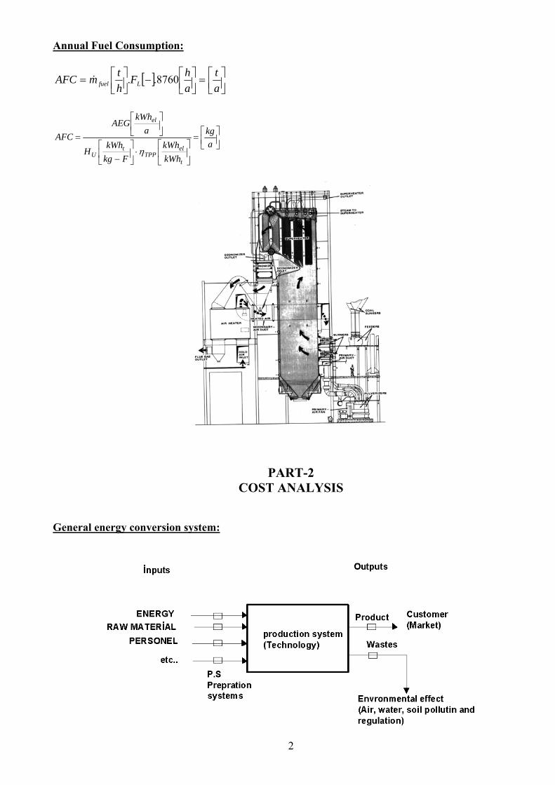
Annual Fuel Consumption:
[ ] ⎥⎦⎤
⎢⎣⎡=⎥⎦
⎤⎢⎣⎡−⎥⎦
⎤⎢⎣⎡=
at
ahF
htmAFC Lfuel 8760..&
⎥⎦⎤
⎢⎣⎡=
⎥⎦
⎤⎢⎣
⎡⋅⎥
⎦
⎤⎢⎣
⎡−
⎥⎦
⎤⎢⎣
⎡
=akg
kWhkWh
FkgkWh
H
akWh
AEGAFC
t
elTPP
tU
el
η
PART-2 COST ANALYSIS
General energy conversion system:

3
General energy production and profit analysis:

4
Profit spoon:
Total Production Cost: OthPersAmrFT CCCCC +++= ⎥⎦
⎤⎢⎣
⎡
elkWhTL
Fuel Cost: ⎥⎦
⎤⎢⎣
⎡⋅⎥⎦
⎤⎢⎣
⎡−
⎥⎦
⎤⎢⎣
⎡−−
=−
−
t
elTPP
tU
F
kWhkWh
FkgkWh
H
FkgFTLg
Cη
⎥⎦
⎤⎢⎣
⎡ −
elkWhFTL
Amortization Cost: ⎥⎦
⎤⎢⎣
⎡
⎥⎦⎤
⎢⎣⎡ −
=
akWh
E
aAmrTLYA
Cel
Amr ⎥⎦
⎤⎢⎣
⎡ −
elkWhAmrTL
Yearly Amortization: [ ] ⎥⎦
⎤⎢⎣⎡−=a
ARAmrTLTICYA 1. ⎥⎦⎤
⎢⎣⎡ −
aAmrTL
Total Investment Cost: [ ] ⎥⎦
⎤⎢⎣
⎡=
elel kW
TLSICkWICTIC . [ ]TL
Amortization Ratio: ( )( ) 11
1−+
+=
A
A
n
n
FFFAR ⎥⎦
⎤⎢⎣⎡a1
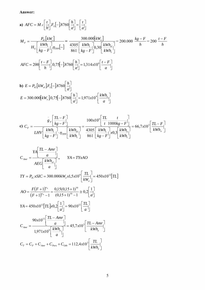
Example 1. For a TPP the following data are given:
PIC=300 MWe, SIC=1,5x10⁹ [TL/kWe], ηTPP=0,30 [kWhe/kWht], Hu=4305 [kcal/kg], gF=100x106 [TL/t], FL=0,75 [-], F=15 [%], nAmr=10 years, nEC=30 years, nphs=40 years, use linear amortization
a) Calculate annual fuel consumption [t/a]. b) Calculate annual electricity generation [kWh/a]. c) Calculate CF [TL- F/kWhel], CAm [TL-Am/kWhel], Cother=0, CT [TL/kWhel]. d) Calculate total profit [TL] in economical life time (Csell=140x103 [TL/kWhe]=constant, CF
increases after nAmr linearly to 115x103 [TL/kWhel] at nEC). e) How can you utilize TPP between nEC and nphy.
5
Answer:
a) [ ] ⎥⎦⎤
⎢⎣⎡=⎥⎦
⎤⎢⎣⎡−⎥⎦
⎤⎢⎣⎡=
at
ahF
htMAFC LF 8760..
.
[ ][ ]−⎥
⎦
⎤⎢⎣
⎡−
=
TPPt
U
tICF
FkgkWhH
kWPMη.
.
= [ ]
⎥⎦
⎤⎢⎣
⎡⎥⎦
⎤⎢⎣
⎡− t
elt
e
kWhkWh
FkgkWh
kW
30,0861
4305000.300 = 200.000
hFkg − = 200
hFt −
[ ] ⎥⎦⎤
⎢⎣⎡ −
=⎥⎦⎤
⎢⎣⎡−⎥⎦
⎤⎢⎣⎡ −
=aFtx
ah
hFtAFC 6
.10314,18760.75,0.200
b) [ ] [ ] ⎥⎦⎤
⎢⎣⎡−=ahFkWPE LelIC 8760..
[ ] [ ] ⎥⎦⎤
⎢⎣⎡=⎥⎦
⎤⎢⎣⎡−=
akWhx
ahkWE e
e910971,18760.75,0.000.300
c) ⎥⎦
⎤⎢⎣
⎡ −=
⎥⎦
⎤⎢⎣
⎡⎥⎦
⎤⎢⎣
⎡−
⎥⎦
⎤⎢⎣
⎡−
=
⎥⎦
⎤⎢⎣
⎡⋅⎥⎦
⎤⎢⎣
⎡−
⎥⎦
⎤⎢⎣
⎡−−
=
−
e
t
et
t
elTPP
t
F
F kWhFTLx
kWhkWhx
FkgkWh
Fkgt
tTLx
kWhkWh
FkgkWhLHV
FkgFTLg
C 3
6
107,663,0
8614305
100010100
η
⎥⎦⎤
⎢⎣⎡
⎥⎦⎤
⎢⎣⎡ −
=
akWh
AEG
aAmrTLYA
Cel
Amr , TYxAOYA =
[ ]TLxkWTLxxkWxSICPTY
eeIC
129 10450105,1000.300 =⎥⎦
⎤⎢⎣
⎡==
( )( ) ⎥⎦
⎤⎢⎣⎡≅
−++
=−+
+=
aFFFAO
A
A
n
n 12,01)115,0(
)115,0(15,011
110
10
[ ] ⎥⎦⎤
⎢⎣⎡=⎥⎦
⎤⎢⎣⎡=
aTLx
axTLxYA 1212 109012,010450
⎥⎦
⎤⎢⎣
⎡ −=
⎥⎦⎤
⎢⎣⎡
⎥⎦⎤
⎢⎣⎡ −
=ee
Amr kWhAmrTLx
akWhx
aAmrTLx
C 3
9
12
107,4510971,1
1090
⎥⎦
⎤⎢⎣
⎡=+++=
eOthPersAmrFT kWh
TLxCCCCC 3104,112

6
d)
[ ] [ ] [ ] [ ] [ ]TLxxxxxxaxna
kWhxEkWhTLCCC Amr
e
eTsellnprofit Amr
12933 105441010971,1104,11210140 =−=⎥⎦⎤
⎢⎣⎡
⎥⎦
⎤⎢⎣
⎡−=−
( ) ( )AmrECFF
Fsellnnofit nnxExCC
CCC nAmrnec
necECAmr−
⎥⎥⎦
⎤
⎢⎢⎣
⎡⎟⎟⎠
⎞⎜⎜⎝
⎛ −+−=−− 2Pr
( ) ( ) [ ]TLxxxxxxxxCECAmr nnofit
15933
33Pr 1094,1103010971,1
2107,66101151011510140 =−⎥
⎦
⎤⎢⎣
⎡⎟⎟⎠
⎞⎜⎜⎝
⎛ −+−=−−
[ ]TLxCCCECAmrAmr nnofitnofittotalofit
15PrPrPr 10484,2=+= −−−−
e) ......Peak Load .....
PART-3
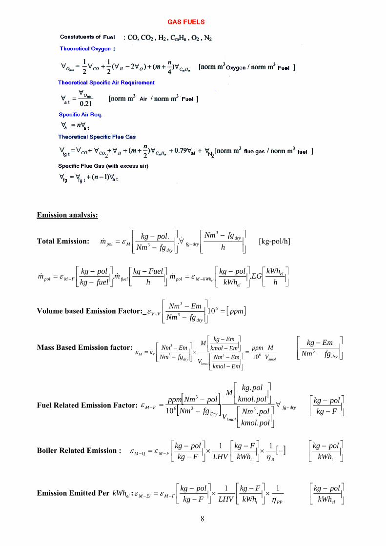
COMBUSTION AND EMISSION ANALYSIS
Combustion analysis:
Fuel Demand: ⎥⎦⎤
⎢⎣⎡
hkg
[ ]
[ ]−⎥⎦
⎤⎢⎣
⎡−
=
Bt
tfuel
FkgkWh
LHV
kWQm
η.
.
&
TL/kWhe
n [a]
CF
CT CAmr
CProfit-nAmr CF=CT
Csell
CPro.-nAmr-nEC

7
[ ]
⎥⎦
⎤⎢⎣
⎡⎥⎦
⎤⎢⎣
⎡−
=
t
elPP
t
elelfuel
kWhkWh
FkgkWh
LHV
kWPm
η.&
Combustion Air Demand:
⎥⎦
⎤⎢⎣
⎡−−
∀⎥⎦⎤
⎢⎣⎡ −
=∀FkgANm
hFkgm afuela
3
.&& [Nm3-A/ h] ⎥⎦
⎤⎢⎣
⎡−−
∀=∀FkgANmn ata
3
. 221
21O
n−
=
Combustion Gas Flow:
⎥⎦
⎤⎢⎣
⎡−−
∀⎥⎦⎤
⎢⎣⎡ −
=∀ −−− FkgGNm
hFkgm wetDryfgfuelwetDryfg
3
.&& ⎥⎥⎦
⎤
⎢⎢⎣
⎡ −h
GNm3
( )
tawetdryfgtwetdryfg n ∀−+∀=∀ −−−− .1 , OHdryfgfg 2∀+∀=∀ −
)9(244.12 HOH mw +=∀ , [Nm3/kg fuel] solid and liquid fuels
)2
(22 nmHCHOH
n∀+∀=∀ , [Nm3/ Nm3fuel] gas fuels
273273.00
3 +∀=⎥
⎦
⎤⎢⎣
⎡∀ −−
Th
mCfgTfg
&&
8
Emission analysis:
Total Emission: ⎥⎥⎦
⎤
⎢⎢⎣
⎡ −∀
⎥⎥⎦
⎤
⎢⎢⎣
⎡
−−
= − hfgNm
fgNmpolkgm dry
dryfgdry
Mpol
3
3 .. && ε [kg-pol/h]
⎥⎦⎤
⎢⎣⎡ −
⎥⎦
⎤⎢⎣
⎡−−
= − hFuelkgm
fuelkgpolkgm fuelFMpol && .ε ⎥⎦
⎤⎢⎣⎡
⎥⎦
⎤⎢⎣
⎡ −= − h
kWhEG
kWhpolkgm el
elkWhMpol el
.ε&
Volume based Emission Factor: [ ]ppmfgNmEmNm
dryVV =
⎥⎥⎦
⎤
⎢⎢⎣
⎡
−−
−6
3
3
10ε
Mass Based Emission factor: kmol
kmoldry
VM VMppm
EmkmolEmNmV
EmkmolEmkgM
fgNmEmNm
633
3
10=
⎥⎦
⎤⎢⎣
⎡−−
⎥⎦⎤
⎢⎣⎡
−−
×⎥⎥⎦
⎤
⎢⎢⎣
⎡
−−
= εε ⎥⎥⎦
⎤
⎢⎢⎣
⎡
−−
dryfgNmEmkg
3
Fuel Related Emission Factor: [ ]
[ ] dryfg
kmolDry
FM
polkmolpolNmV
polkmolpolkgM
fgNmpolNmppm
−− ∀
⎥⎦
⎤⎢⎣
⎡
⎥⎦
⎤⎢⎣
⎡
−−
=
.
..
.
10 336
3
ε ⎥⎦
⎤⎢⎣
⎡−−
Fkgpolkg
Boiler Related Emission : [ ]−×⎥⎦
⎤⎢⎣
⎡ −×⎥⎦
⎤⎢⎣
⎡−−
= −−Bt
FMQM kWhFkg
LHVFkgpolkg
ηεε 11 ⎥
⎦
⎤⎢⎣
⎡ −
tkWhpolkg
Emission Emitted Per elkWh :PPt
FMElM kWhFkg
LHVFkgpolkg
ηεε 11
×⎥⎦
⎤⎢⎣
⎡ −×⎥
⎦
⎤⎢⎣
⎡−−
= −− ⎥⎦
⎤⎢⎣
⎡ −
elkWhpolkg

9
Example 2. Make the following emission calculations for the TPP given in Example 1. The following data is given: SO2=2000 [ppm], O2=7 [%], VHth=VGth-dry=5 [Nm3/kg-F].
a) Calculate εSOel [kg-SO2/kWhel]. b) Calculate annual SO2 emission ASO2 [t-SO2/a].
Answer: a)
[ ][ ] ⎥
⎦
⎤⎢⎣
⎡ −=⎥
⎦
⎤⎢⎣
⎡⎥⎦
⎤⎢⎣
⎡ −
⎥⎥⎦
⎤
⎢⎢⎣
⎡
−
−∀
⎥⎦
⎤⎢⎣
⎡
⎥⎦
⎤⎢⎣
⎡
−−
= −−ee
t
TPPtu
Drydryfg
kmolDry
elSO kWhSOkg
kWhkWh
kWhFkg
HFkgfgNm
SOkmolSONmV
SOkmolSOkgM
fgNmSONmppm 2
3
2
23
2
2
362
3 11
..
..
102 ηε
5,1721
21=
−=n
( ) ⎥⎦
⎤⎢⎣
⎡−
=−+=∀−+∀=∀ −−−−−− Fkg
Nmn wetdryfgatwetdryfgtwetdryfg
3
5,7)15,1(5.1
[ ][ ] ⎥
⎦
⎤⎢⎣
⎡⎥⎦
⎤⎢⎣
⎡ −
⎥⎥⎦
⎤
⎢⎢⎣
⎡
−
−
⎥⎦
⎤⎢⎣
⎡
⎥⎦
⎤⎢⎣
⎡
−−
=−e
t
t
Dry
DryelSO kWh
kWhkWh
FkgxFkgfgNm
SOkmolSONm
SOkmolSOkg
fgNmSONmppm
3,01
8614305
15,7
.
.4,22
..64
10200 3
2
23
2
2
362
3
2ε
⎥⎦
⎤⎢⎣
⎡ −=−
eelSO kWh
SOkg 202857,02
ε
b)
⎥⎦
⎤⎢⎣
⎡−−
⎥⎦⎤
⎢⎣⎡
⎥⎦
⎤⎢⎣
⎡ −=⎥⎦
⎤⎢⎣⎡
⎥⎦
⎤⎢⎣
⎡ −=− −
2
29222 1000
110971,102857,02 SOkg
SOta
kWhxxkWh
SOkga
kWhxEkWh
SOkgSOA e
e
e
eelSOε
⎥⎦⎤
⎢⎣⎡ −
=−aSOtSOA 2
2 5,56311
10
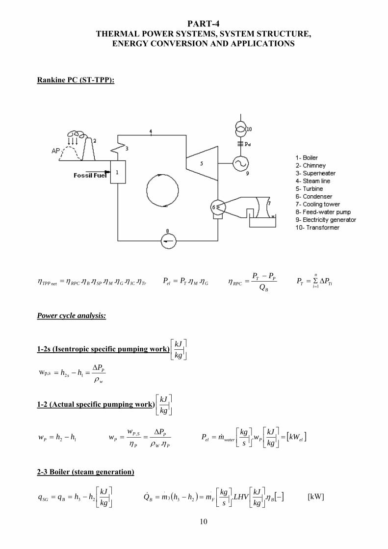
PART-4 THERMAL POWER SYSTEMS, SYSTEM STRUCTURE,
ENERGY CONVERSION AND APPLICATIONS Rankine PC (ST-TPP):
TrICGMSPBRPCnetTPP ηηηηηηηη ......= GMTel PP ηη ..= B
PTRPC Q
PP −=η Ti
n
iT PP ΔΣ==1
Power cycle analysis:
1-2s (Isentropic specific pumping work) ⎥⎦
⎤⎢⎣
⎡kgkJ
wp,s 12 hh s −=w
PPρΔ
=
1-2 (Actual specific pumping work) ⎥⎦
⎤⎢⎣
⎡kgkJ
12 hhwP −= PW
P
P
SPP
Pww
ηρη ., Δ== [ ]elPwaterel kW
kgkJw
skgmP =⎥
⎦
⎤⎢⎣
⎡⎥⎦⎤
⎢⎣⎡= .&
2-3 Boiler (steam generation)
⎥⎦
⎤⎢⎣
⎡−==
kgkJhhqq BSG 23 ( ) [ ]−⎥
⎦
⎤⎢⎣
⎡⎥⎦⎤
⎢⎣⎡=−= BFB kg
kJLHVs
kgmhhmQ η...
233
.& [kW]

11
3-4 Specific Turbine work
sST hhw 43. −= STTT whhw ,43 .η=−= s
T hhhh
43
43
−−
=η
4-1 Condensation (Condenser)
14 hhqCond −= AprCOCond TTT Δ+= CTCiCO TTT +=
Steam generation process analysis:
SHEVPHSG qqqq ++= 22 hhqPH −= ′ 22 ′′′ −= hhqEV 23 ′′−= hhqSH
Reheat Pressure:
( )2323 SSThhq mSG −=−=−

12

13
General Rankine power cycle thermal power plants:
14

15
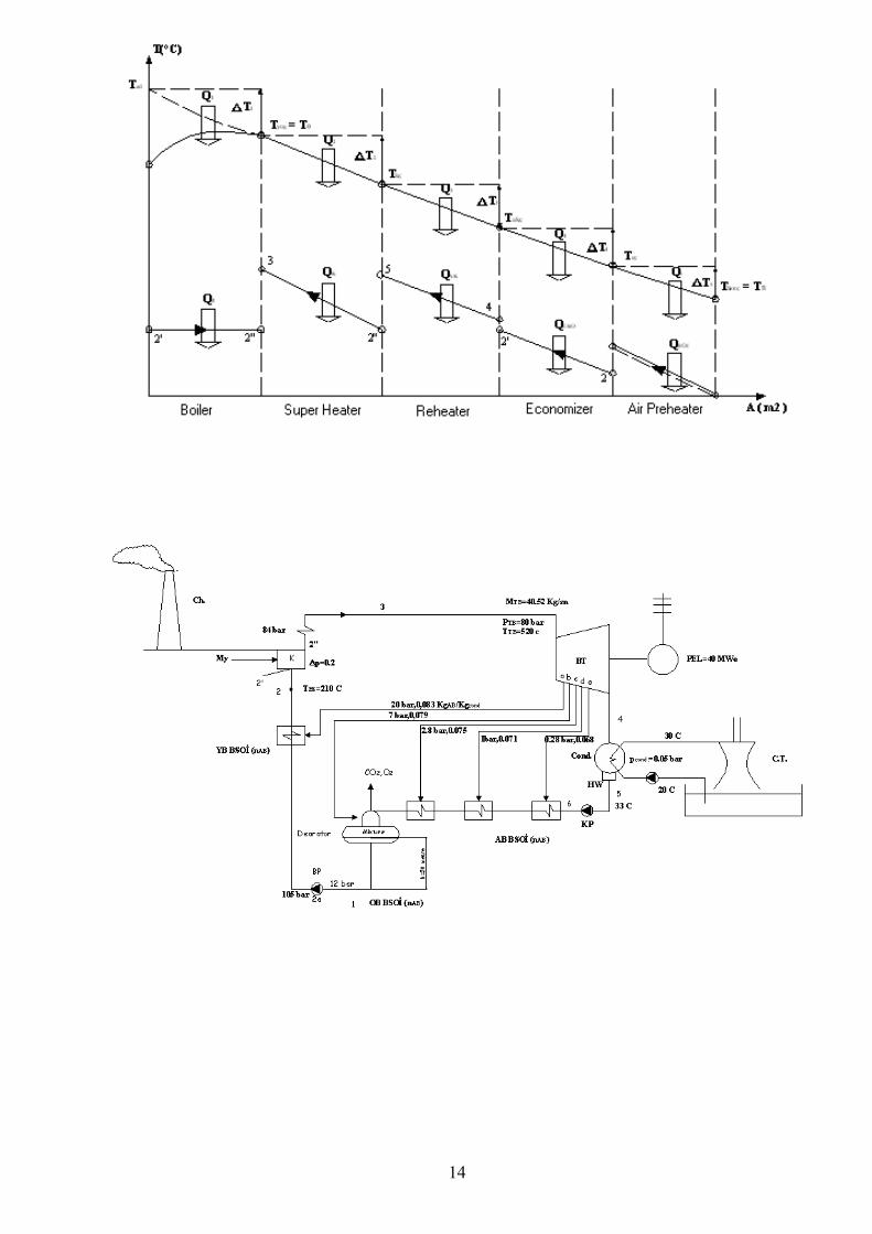
Example 3. The flow diagram of a TPP- steam power cycle is given below. Answer: a)
a) Sketch the steam power cycle on h-s diagram. b) Calculate the extraction pressures Pex4 - Pex6 (bar) and extraction steam mass flow rates m4 – m6 [kg/s] ( ΔTAPP = 5 ° C) c) Calculate PelGR [MWe] (ηM= 1, ηG= 0.98, x7 = 0.95 ) d) Calculate mCW [t/h] and mCW / m3
(CPW= 4.18 kj/kg0C) e) Calculate the fuel consumption MF [t/h] (Hu = 5 kWht / kg-F , ηB= 0.85)
~
∆TP=0
MF
3
4
2 Pex 4 35 ° C
22 ° C mCW
PelGr
5 6
550 ° C 360 [t/h] 100 [bar]
1
200 ° C 150 ° C 100 ° C
7
8
CT
9 10 11
m4= 0.05 m3 m5= 0.10 m3 m6= 0.15 m3
38 ° C
∆TP=0
16
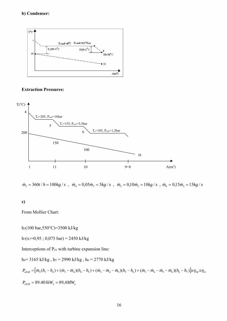
b) Condenser:
Extraction Pressures:
skghtm /100/3603 ==& , skgmm /505,0 34 == && , skgmm /1010,0 35 == && , skgmm /1515,0 36 == && c) From Mollier Chart: h3(100 bar,550°C)=3500 kJ/kg h7(x7=0,95 ; 0,075 bar) = 2450 kJ/kg Interceptions of Pex with turbine expansion line: h4= 3165 kJ/kg , h5 = 2990 kJ/kg , h6 = 2770 kJ/kg
[ ] GMelGR xxhhmmmmhhmmmhhmmhhmP ηη))(())(())(()( 766543655435443433 −−−−+−−−+−−+−= &&&&&&&&&&
eeelGR MWkWP 4,89401.89 ==
38100
150
200
Tc=205, Pex4=16bar
6
5
4
Tc=155, Pex5=5,5bar
Tc=105, Pex6=1,2bar
11 10 9=81
T(°C)
A(m2)
17
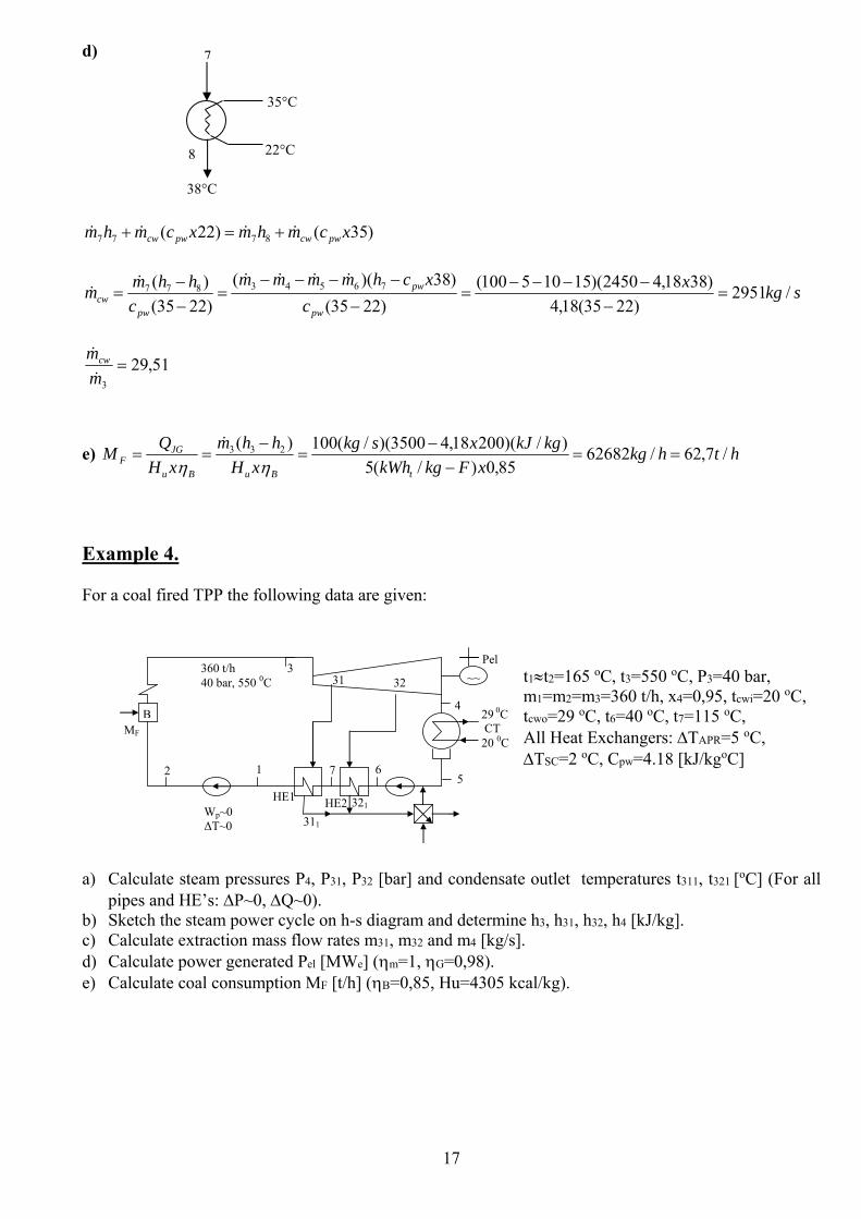
d)
)35()22( 8777 xcmhmxcmhm pwcwpwcw &&&& +=+
skgxc
xchmmmmc
hhmmpw
pw
pwcw /2951
)2235(18,4)3818,42450)(15105100(
)2235()38)((
)2235()( 76543877 =
−−−−−
=−
−−−−=
−−
=&&&&&
&
51,293
=mmcw
&
&
e) hthkgxFkgkWh
kgkJxskgxH
hhmxH
QMtBuBu
JGF /7,62/62682
85,0)/(5)/)(20018,43500)(/(100)( 233 ==
−−
=−
==ηη
&
Example 4. For a coal fired TPP the following data are given:
t1≈t2=165 oC, t3=550 oC, P3=40 bar, m1=m2=m3=360 t/h, x4=0,95, tcwi=20 oC, tcwo=29 oC, t6=40 oC, t7=115 oC, All Heat Exchangers: ΔTAPR=5 oC, ΔTSC=2 oC, Cpw=4.18 [kJ/kgoC]
a) Calculate steam pressures P4, P31, P32 [bar] and condensate outlet temperatures t311, t321 [oC] (For all
pipes and HE’s: ΔP~0, ΔQ~0). b) Sketch the steam power cycle on h-s diagram and determine h3, h31, h32, h4 [kJ/kg]. c) Calculate extraction mass flow rates m31, m32 and m4 [kg/s]. d) Calculate power generated Pel [MWe] (ηm=1, ηG=0,98). e) Calculate coal consumption MF [t/h] (ηB=0,85, Hu=4305 kcal/kg).
7
38°C
35°C
22°C 8
360 t/h 3 40 bar, 550 0C
Wp~0 ΔT~0
B
1
2
7
6
4
5 HE1
29 0C CT 20 0C
~~ 31 32
MF
Pel
HE2 311
321

18
Answer: a)
b)
19
kgkjhkgkjhkgkjh
kgkjbarCh
/2565/2925/3195
/3560)40,550(
4
32
31
03
===
=
c)
skgmmmm
skgm
skgskgm
hhmhhmskghtmmmmm
/73.78
/89.1211818.42925
)40115(18.4100
/38.816818.43195
)115165(18.4/100
)()(/100/360
323134
32
31
343131177
67321
=−−=
=×−−×
=
=×−−×
=
−=−======
&&&&
&
&
&&
Pel= [ m& 3(h3-h31) + ( m& 3- m& 31)(h31-h32) + ( m& 3- m& 31- m& 32)(h32-h4)] . ηM.ηG
=100(3560-3195) + ( 100-8.38) (3195-2925) + (100-8.38-12.89) (2925-2565) Pel=89.6 MWel d)
[ ]htM
skgkcalkjkgkcal
kgkjskgM
hhmHM
F
F
BuF
/6.67
/77.1885.0/18.4/4305
/)16518.43560(/100)( 233
=
=××
×−=
−=
&
&
&& η

20
Brayton Power Cycle (GT-TPP):
( ) GMCTGelGT wwmP ηη ..Σ−Σ=− & CC
CTBPC q
ww −=η GMCCBPCGTnet
ηηηηη ...=
1-2s (Isentropic Compression work) ⎥⎦
⎤⎢⎣
⎡kgkJ
⎥⎥⎥
⎦
⎤
⎢⎢⎢
⎣
⎡−⎟⎟
⎠
⎞⎜⎜⎝
⎛=−=
−
1..
1
1
21112,
kk
psSC PPTchhw ( )12, 21 ttCw SPSC S −= −
−
1-2( Poly. Comp. Work)
( )12,
12 21 ttCw
hhw P
C
SCC −==−= −
−
η ⎥
⎦
⎤⎢⎣
⎡⎥⎦⎤
⎢⎣⎡=
kgkJw
skgmP CGCom .& [kW]
2-3 (Heat Gen.)
23 hhqCC −= ⎥⎦
⎤⎢⎣
⎡kgkJ ( )2323 ttCq pCC −=
−
3-4s (Isent. Exp. Process)
( )sPsST ttChhw s 4343, 43 −=−= −
−
⎥⎥⎥
⎦
⎤
⎢⎢⎢
⎣
⎡
⎥⎦
⎤⎢⎣
⎡−=
−k
k
PST PPTcw
1
3
433, 1.. [kJ/kg]
3-4(Poly.Exp.Work)
( ) STTPT wttChhw ,4343 .43 η=−=−= −
−
[kJ/kg]
21
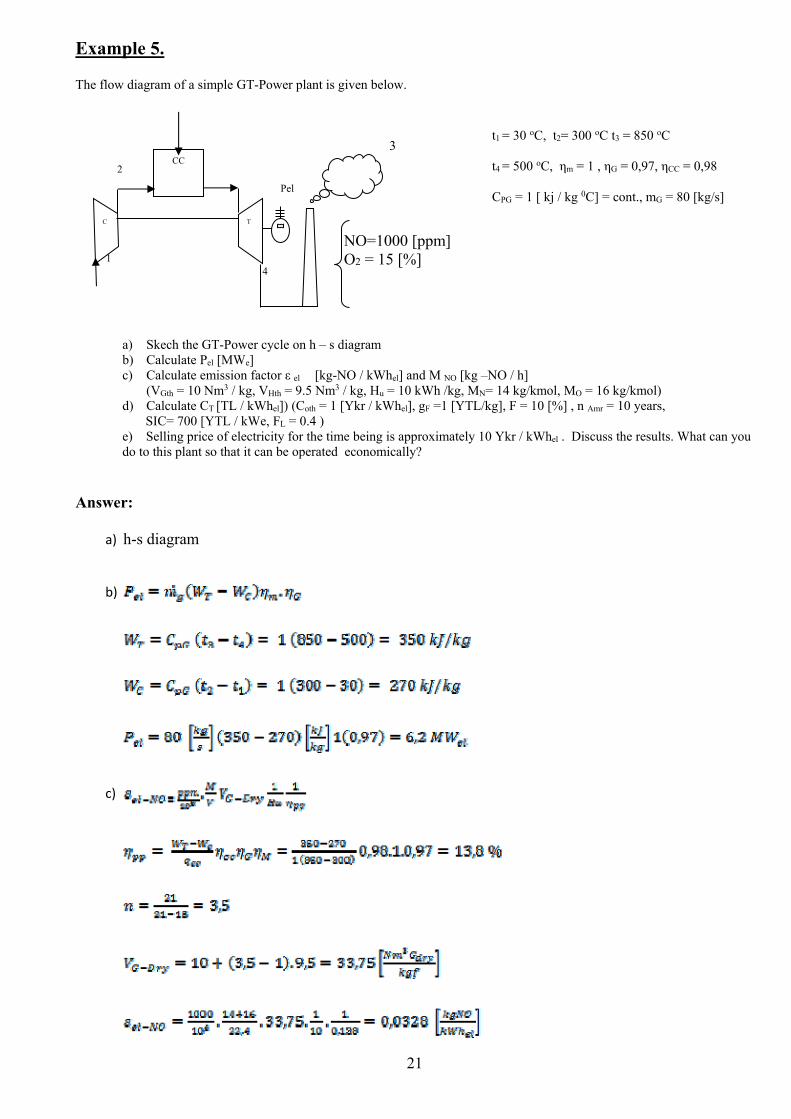
Example 5. The flow diagram of a simple GT-Power plant is given below. 3
a) Skech the GT-Power cycle on h – s diagram b) Calculate Pel [MWe] c) Calculate emission factor ε el [kg-NO / kWhel] and M NO [kg –NO / h]
(VGth = 10 Nm3 / kg, VHth = 9.5 Nm3 / kg, Hu = 10 kWh /kg, MN= 14 kg/kmol, MO = 16 kg/kmol) d) Calculate CT [TL / kWhel]) (Coth = 1 [Ykr / kWhel], gF =1 [YTL/kg], F = 10 [%] , n Amr = 10 years, SIC= 700 [YTL / kWe, FL = 0.4 ) e) Selling price of electricity for the time being is approximately 10 Ykr / kWhel . Discuss the results. What can you do to this plant so that it can be operated economically?
Answer:
a) h-s diagram
b)
c)
2
C T
1 4
CC
Pel
NO=1000 [ppm] O2 = 15 [%]
t1 = 30 oC, t2= 300 oC t3 = 850 oC t4 = 500 oC, ηm = 1 , ηG = 0,97, ηCC = 0,98 CPG = 1 [ kj / kg 0C] = cont., mG = 80 [kg/s]
22
d) �
e) ...............
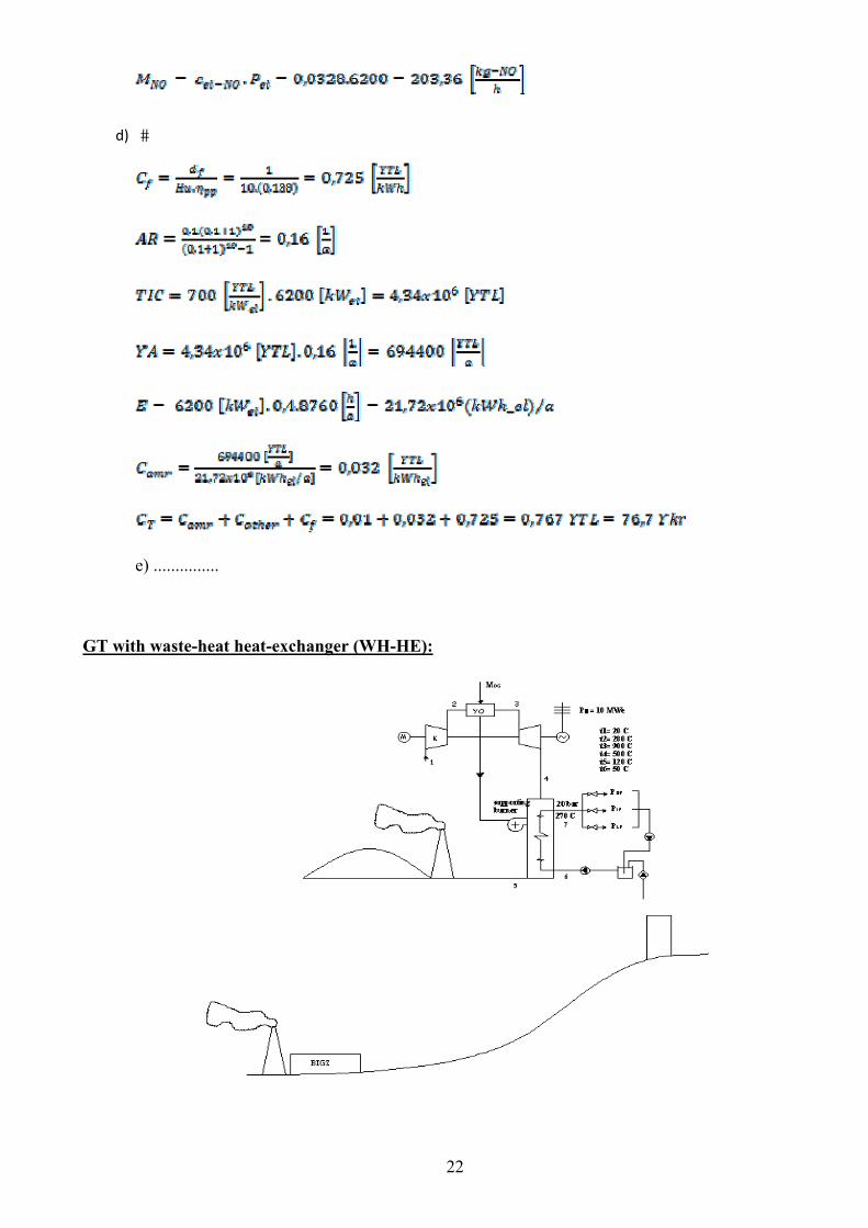
GT with waste-heat heat-exchanger (WH-HE):
23
24
22
TTTT ı
HEWH −−
=−η
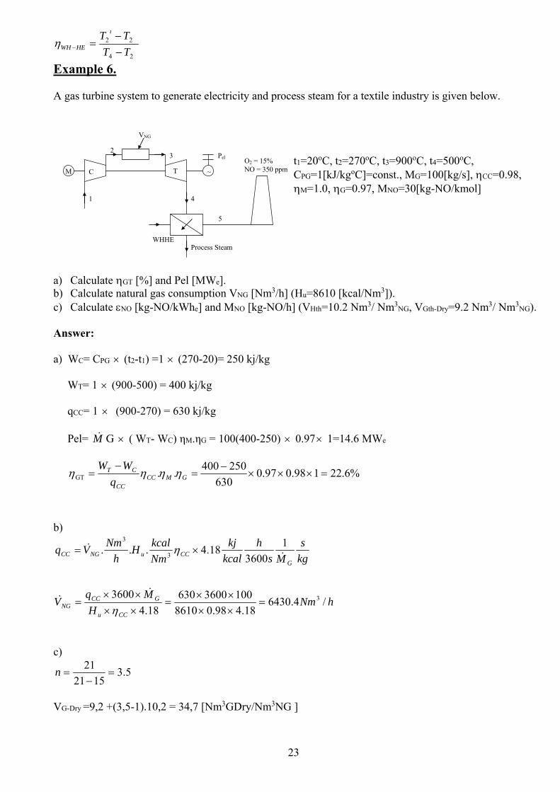
Example 6. A gas turbine system to generate electricity and process steam for a textile industry is given below.
t1=20oC, t2=270oC, t3=900oC, t4=500oC, CPG=1[kJ/kgoC]=const., MG=100[kg/s], ηCC=0.98, ηM=1.0, ηG=0.97, MNO=30[kg-NO/kmol]
a) Calculate ηGT [%] and Pel [MWe]. b) Calculate natural gas consumption VNG [Nm3/h] (Hu=8610 [kcal/Nm3]). c) Calculate εNO [kg-NO/kWhe] and MNO [kg-NO/h] (VHth=10.2 Nm3/ Nm3NG, VGth-Dry=9.2 Nm3/ Nm3NG). Answer: a) WC= CPG × (t2-t1) =1 × (270-20)= 250 kj/kg WT= 1 × (900-500) = 400 kj/kg qCC= 1 × (900-270) = 630 kj/kg Pel= M& G × ( WT- WC) ηM.ηG = 100(400-250) × 0.97× 1=14.6 MWe
%6.22198.097.0630
250400..GT =×××−
=−
= GMCCCC
CT
qWW
ηηηη
b)
hNmH
MqV
kgs
Msh
kcalkj
NmkcalH
hNmVq
CCu
GCCNG
GCCuNGCC
/4.643018.498.08610
100360063018.4
3600
13600
18.4...
3
3
3
=××××
=××××
=
×=
η
η
&&
&&
c)
5.31521
21=
−=n
VG-Dry =9,2 +(3,5-1).10,2 = 34,7 [Nm3GDry/Nm3NG ]
O2 = 15% NO = 350 ppm M C
1
2
T
Pel
~
WHHE Process Steam
3
4
VNG
5

24
.
GT with Reheat
M
CT
WW
η=
1 ( ) GMTGGT wmP ηη ..
2&= GM
cc
cc
cc
cc
TGT qq
wηη
ηη
η ..
2
2
1
1
2
+=
Co-Generation PP:
LHVmQP
F
IndelCPP .&
&+=η
Combined Cycle PP
25
LHVmPP
F
STelGTelCCPP .&
−− +=η
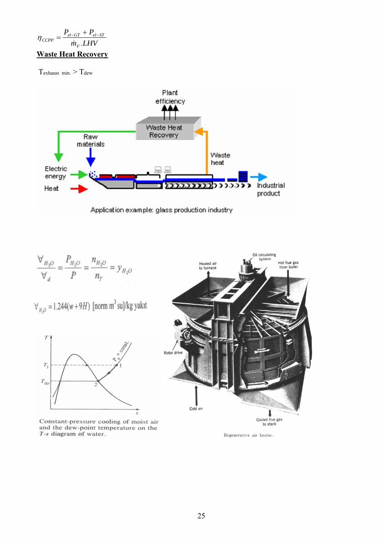
Waste Heat Recovery Texhaust min. > Tdew
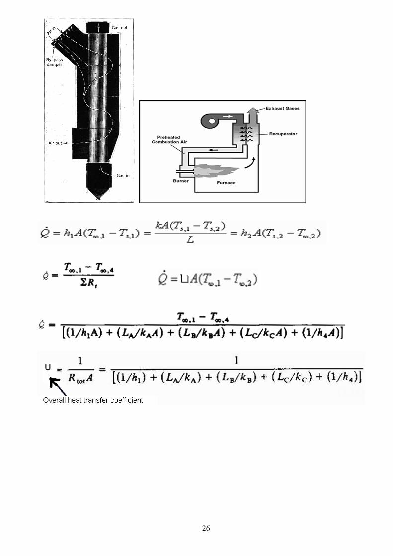
26
27
28
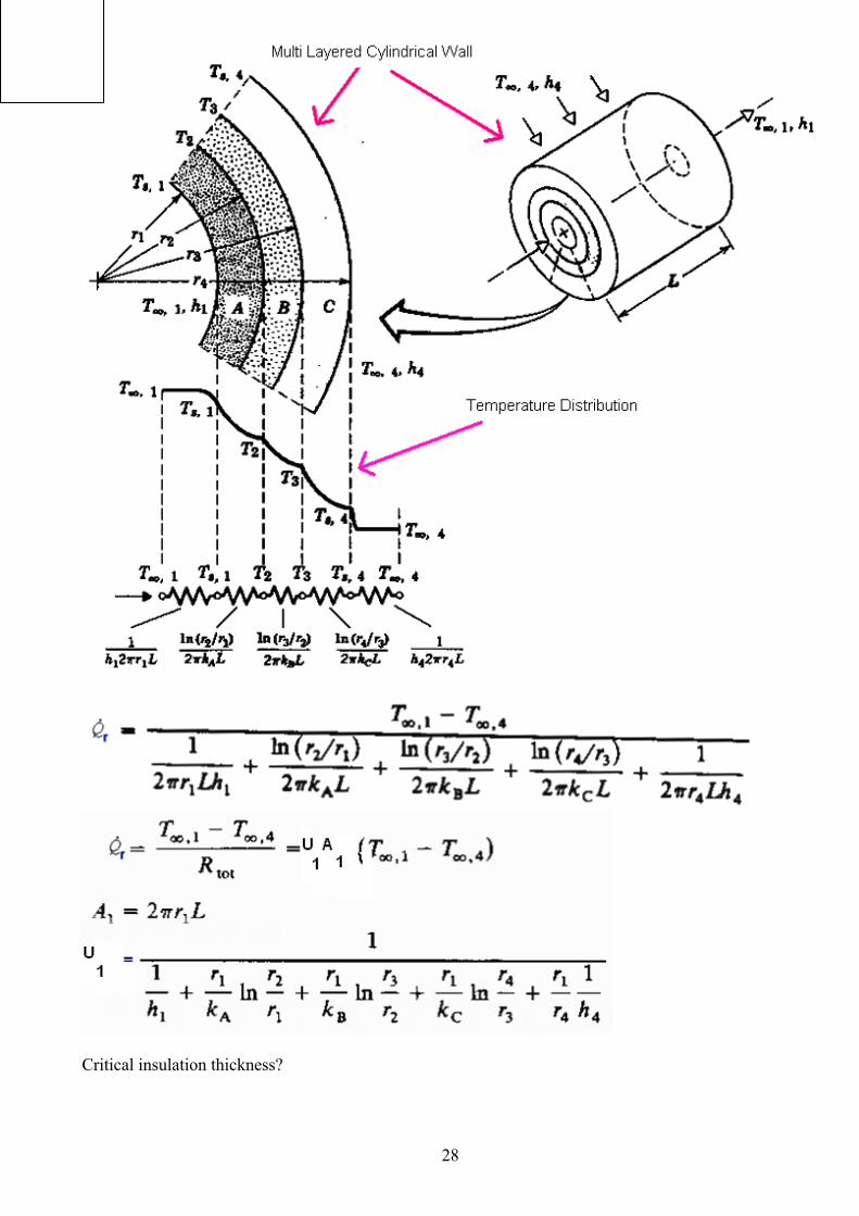
Critical insulation thickness?
Related Documents