Compiling Stan to Generative Probabilistic Languages ... - arXiv

Compiling Stan to Generative Probabilistic Languagesand Extension to Deep Probabilistic Programming

Guillaume Baudart

INRIA Paris

École normale supérieure – PSL University

France

Javier Burroni

UMass Amherst

USA

Martin Hirzel

MIT-IBM Watson AI Lab, IBM Research

USA

Louis Mandel

MIT-IBM Watson AI Lab, IBM Research

USA

Avraham Shinnar

MIT-IBM Watson AI Lab, IBM Research

USA

AbstractStan is a probabilistic programming language that is popu-

lar in the statistics community, with a high-level syntax for

expressing probabilistic models. Stan differs by nature from

generative probabilistic programming languages like Church,

Anglican, or Pyro. This paper presents a comprehensive com-

pilation scheme to compile any Stan model to a generative

language and proves its correctness. We use our compilation

scheme to build two new backends for the Stanc3 compiler

targeting Pyro and NumPyro. Experimental results show

that the NumPyro backend yields a 2.3x speedup compared

to Stan in geometric mean over 26 benchmarks. Building on

Pyro we extend Stan with support for explicit variational

inference guides and deep probabilistic models. That way,

users familiar with Stan get access to new features without

having to learn a fundamentally new language.

CCS Concepts: • Software and its engineering→ Com-pilers; • Theory of computation→ Probabilistic com-putation.

Keywords: Probabilistic programming, Semantics, Stan, Pyro

1 IntroductionProbabilistic Programming Languages (PPLs) are designed

to describe probabilistic models and run inference on them.

There exists a variety of PPLs. BUGS [21], JAGS [26], and

Stan [7] focus on efficiency, constraining what is expressible

to a subset of models which support fast inference techniques.

These languages enjoy broad adoption by the statistics and

social sciences communities [6, 10, 11]. Generative languageslike Church [12], Anglican [32], WebPPL [13], Pyro [3], and

Gen [9] describe generative models, i.e., stochastic proceduresthat simulate the data generation process. Coming from a

core programming languages heritage, generative PPLs typi-

cally support rich control constructs and models over struc-

tured data. Generative PPLs are increasingly used inmachine-

learning research and are rapidly incorporating new ideas,

such as Stochastic Gradient Variational Inference (SVI), in

what is now called Deep Probabilistic Programming [2, 3, 33].

While the semantics of probabilistic languages have been

extensively studied [14, 15, 18, 30], to the best of our knowl-

edge little is known about the relationship between Stan and

generative PPLs. We show that a simple 1:1 translation is

incorrect or incomplete for a set of subtle but widely-used

Stan features, such as left expressions or implicit priors.

This paper formalizes the relationship between Stan and

generative PPLs and introduces, with correctness proof, a

comprehensive compilation scheme that can compile any

Stan program to a generative PPL. This enables leverag-

ing the rich set of existing Stan models for testing, bench-

marking, or experimenting with new features or inference

techniques. Based on this compilation scheme we imple-

mented two new backends for the Stanc3 compiler target-

ing Pyro [3] and NumPyro [25], a JAX [5] based version of

Pyro. Both Pyro and NumPyro runtimes offer NUTS [16] (No

U-Turn Sampler), an optimized Hamiltonian Monte-Carlo

(HMC) algorithm that is the preferred inference method for

Stan. We can thus validate our approach against Stan. Re-

sults show that models compiled using our NumPyro back-

end yield equivalent results while being 2.3x faster than

1

arX

iv:1

810.

0087

3v5

[cs

.LG

] 1

1 A

pr 2

021

their Stan counterpart in the geometric mean over 26 bench-

marks. Our compiler and runtime library are open-source at

https://github.com/deepppl.In addition, recent probabilistic languages offer new fea-

tures to program and reason about complex models. Our

compilation scheme combined with conservative extensions

of Stan can be used to make these benefits available to Stan

users. As a proof of concept, based on our Pyro backend,

this paper introduces DeepStan: Stan extended with sup-

port for explicit variational guides and deep probabilistic

models. Variational inference was central in the design of

Pyro and programmers can easily craft their own inference

guides to run variational inference on probabilistic mod-

els. Pyro is built on top of PyTorch [24]. Programmers can

thus seamlessly import neural networks designed with the

state-of-the-art API provided by PyTorch.

This paper makes the following contributions:

• A comprehensive compilation scheme from Stan to a gen-

erative PPL (Section 2).

• Correctness proof of the compilation scheme (Section 3).

• An open-source implementation of two new backends for

Stanc3 targeting Pyro and NumPyro (Section 4).

• An extension of Stan with explicit variational inference

guides and deep probabilistic models (Section 5).

The fundamental new result of this paper is that every Stan

program can be expressed as a generative probabilistic pro-

gram. Besides advancing the understanding of probabilistic

programming languages at a fundamental level, this paper

aims to provide practical benefits to the communities of both

Stan and Pyro. From the perspective of the Stan community,

this paper presents a new competitive compiler backend and

additional capabilities while retaining familiar syntax and

semantics. This compiler can thus be used to migrate existing

Stan codebases to Pyro and NumPyro. From the perspective

of the Pyro community, this paper presents a new compiler

frontend that unlocks many existing real-world models as

examples and benchmarks.

This paper is a version with appendices presenting the

proofs and the evaluation results of the paper published at

PLDI 2021 [1].

2 OverviewThis section shows how to compile Stan [7], which specifies a

joint probability distribution, to a generative PPL like Church,

Anglican, or Pyro. This translation also demonstrates that

Stan’s expressive power is at most as large as that of genera-

tive languages, a fact that was not clear before our paper.

As a running example, consider the biased coin model in

Figure 1. Stan’s data block defines observed variables for 𝑁

coin flips 𝑥𝑖 , 𝑖 ∈ [1 : 𝑁 ], which can be 0 for tails or 1 for heads.The parameters block introduces a latent variable 𝑧 ∈ [0, 1]for the bias of the coin. The model block sets the prior of

the bias 𝑧 to Beta(1, 1), i.e., a uniform distribution over [0, 1].

data {int N;int<lower=0,upper=1> x[N]; }

parameters {real<lower=0,upper=1> z; }

model {z ~ beta(1, 1);for (i in 1:N) x[i] ~ bernoulli(z); }

𝑧 𝑥

𝑁𝑝 (𝑧 | 𝑥1, . . . , 𝑥𝑁 )

Figure 1. Biased coin model in Stan.

def model(N, x):z = sample(

beta(1.,1.))for i in range(0, N):

observe(bernoulli(z), x[i])

return z

(a) Generative scheme

def model(N, x):z = sample(uniform(0.,1.))observe(beta(1.,1.), z)for i in range(0, N):

observe(bernoulli(z), x[i])

return z

(b) Comprehensive scheme

Figure 2. Compiled coin model of Figure 1.

The for loop indicates that coin flips 𝑥𝑖 are independent and

identically distributed (IID) and depend on 𝑧 via a Bernoulli

distribution. Given concrete observed coin flips, inference

yields a posterior distribution for 𝑧 conditioned on 𝑥1, . . . , 𝑥𝑁 .

2.1 Generative translationGenerative PPLs are general-purpose languages extended

with two probabilistic constructs [14, 30, 34]: sample(𝐷)generates a sample from a distribution 𝐷 and factor(𝑣)assigns a score 𝑣 to the current execution trace. Typically,

factor is used to condition the model on input data [32].

We also introduce observe(𝐷,𝑣) as a syntactic shortcut

for factor(𝐷pdf(𝑣)) where 𝐷pdf denotes the probability

density function of 𝐷 . This construct penalizes executions

according to the score of 𝑣 w.r.t. 𝐷 which captures the as-

sumption that the observed data 𝑣 follows the distribution 𝐷 .

Compilation. Stan uses the same syntax v ~ 𝐷 for both

observed and latent variables. The distinction comes from

the kind of the left-hand-side variable: observed variables are

declared in the data block, latent variables are declared in theparameters block. A straightforward generative translationcompiles a statement v ~ 𝐷 into v = sample(𝐷) if v is

a parameter or observe(𝐷, v) if v is data. For example,

Figure 2a shows the compiled (using the generative scheme)

version of the Stan model of Figure 1 in Python syntax.

2.2 Non-generative featuresIn Stan, a model represents the unnormalized density of the

joint distribution of the parameters defined in the parametersblock given the data defined in the data block [7, 15]. A Stan

program can thus be viewed as a function from parameters

and data to the value of a special variable target that rep-resents the log-density of the model. A Stan model can be

2

Compiling Stan to Generative Probabilistic Languages and Extension to Deep Probabilistic Programming

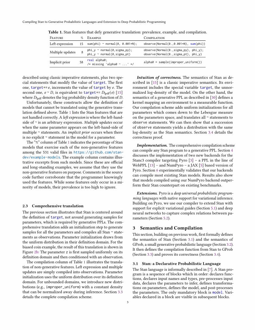
Table 1. Stan features that defy generative translation: prevalence, example, and compilation.

Feature % Example Compilation

Left expression 15 sum(phi) ~ normal(0, 0.001*N); observe(Normal(0.,0.001*N), sum(phi))

Multiple updates 8

phi_y ~ normal(0,sigma_py);phi_y ~ normal(0,sigma_pt)

observe(Normal(0.,sigma_py), phi_y);observe(Normal(0.,sigma_pt), phi_y)

Implicit prior 58

real alpha0;/* missing 'alpha0 ~ ...' */

alpha0 = sample(improper_uniform())

described using classic imperative statements, plus two spe-

cial statements that modify the value of target. The firstone, target+= 𝑒 , increments the value of target by 𝑒 . Thesecond one, e ~ D, is equivalent to target+= 𝐷lpdf (e) [15]where𝐷lpdf denotes the log probability density function of𝐷 .

Unfortunately, these constructs allow the definition of

models that cannot be translated using the generative trans-

lation defined above. Table 1 lists the Stan features that are

not handled correctly. A left expression is where the left-hand-side of ~ is an arbitrary expression. Multiple updates occurwhen the same parameter appears on the left-hand-side of

multiple ~ statements. An implicit prior occurs when there

is no explicit ~ statement in the model for a parameter.

The “%” column of Table 1 indicates the percentage of Stan

models that exercise each of the non-generative features

among the 531 valid files in https://github.com/stan-dev/example-models. The example column contains illus-

trative excerpts from such models. Since these are official

and long-standing examples, we assume that they use the

non-generative features on purpose. Comments in the source

code further corroborate that the programmer knowingly

used the features. While some features only occur in a mi-

nority of models, their prevalence is too high to ignore.

2.3 Comprehensive translationThe previous section illustrates that Stan is centered around

the definition of target, not around generating samples for

parameters, which is required by generative PPLs. The com-

prehensive translation adds an initialization step to generate

samples for all the parameters and compiles all Stan ~ state-

ments as observations. Parameter initialization draws from

the uniform distribution in their definition domain. For the

biased coin example, the result of this translation is shown in

Figure 2b: The parameter z is first sampled uniformly on its

definition domain and then conditioned with an observation.

The compilation column of Table 1 illustrates the transla-

tion of non-generative features. Left expression and multiple

updates are simply compiled into observations. Parameter

initialization uses the uniform distribution over its definition

domain. For unbounded domains, we introduce new distri-

butions (e.g., improper_uniform) with a constant density

that can be normalized away during inference. Section 3.3

details the complete compilation scheme.

Intuition of correctness. The semantics of Stan as de-

scribed in [15] is a classic imperative semantics. Its envi-

ronment includes the special variable target, the unnor-

malized log-density of the model. On the other hand, the

semantics of a generative PPL as described in [30] defines a

kernel mapping an environment to a measurable function.

Our compilation scheme adds uniform initializations for all

parameters which comes down to the Lebesgue measure

on the parameters space, and translates all ~ statements to

observe statements. We can then show that a succession

of observe statements yields a distribution with the same

log-density as the Stan semantics. Section 3.4 details the

correctness proof.

Implementation. The comprehensive compilation scheme

can compile any Stan program to a generative PPL. Section 4

discusses the implementation of two new backends for the

Stanc3 compiler targeting Pyro [3] – a PPL in the line of

WebPPL [13] – and NumPyro – a JAX [5] based version of

Pyro. Section 6 experimentally validates that our backends

can compile most existing Stan models. Results also show

that models compiled using our NumPyro backend outper-

form their Stan counterpart on existing benchmarks.

Extensions. Pyro is a deep universal probabilistic program-ming languages with native support for variational inference.

Building on Pyro, we use our compiler to extend Stan with

support for explicit variational guides (Section 5.1) and deep

neural networks to capture complex relations between pa-

rameters (Section 5.2).

3 Semantics and CompilationThis section, building on previouswork, first formally defines

the semantics of Stan (Section 3.1) and the semantics of

GProb, a small generative probabilistic language (Section 3.2).

It then defines the compilation function from Stan to GProb

(Section 3.3) and proves its correctness (Section 3.4).

3.1 Stan: a Declarative Probabilistic LanguageThe Stan language is informally described in [7]. A Stan pro-

gram is a sequence of blocks which in order: declares func-

tions, declares input names and types, pre-processes input

data, declares the parameters to infer, defines transforma-

tions on parameters, defines the model, and post-processes

the parameters. The only mandatory block is model. Vari-ables declared in a block are visible in subsequent blocks.

3

program ::= functions {fundecl∗} ?data {decl∗} ?

transformed data {decl∗ stmt} ?

parameters {decl∗} ?

transformed parameters {decl∗ stmt} ?

model {decl∗ stmt}generated quantities {decl∗ stmt} ?

Variable declarations (decl∗) are lists of variables names

with their types (e.g., int N;) or arrays with their type and

shape (e.g., real x[N]). Types can be constrained to spec-

ify the domain of a variable (e.g., real <lower=0> x for

𝑥 ∈ R+). Note that vector and matrix are primitive types

that can be used in arrays (e.g. vector[N] x[10] is an array

of 10 vectors of size N). Shapes and sizes of arrays, matrices,

and vectors are explicit and can be arbitrary expressions.

decl ::= base_type constraint 𝑥 ;

| base_type constraint 𝑥 [shape] ;base_type ::= real | int

| vector[size] | matrix[size,size]constraint ::= Y | < lower = 𝑒 , upper = 𝑒 >

| < lower = 𝑒 > | < upper = 𝑒 >shape ::= size | shape , sizesize ::= e

Inside a block, Stan is similar to a classic imperative lan-

guage, with two extra, specialized statements: target += 𝑒directly updates the log-density of the model (stored in the re-

served variable target), and 𝑥 ~𝐷 indicates that a variable 𝑥

follows a distribution 𝐷 .

stmt ::= 𝑥 = 𝑒 variable assignment

| 𝑥[𝑒1,...,𝑒𝑛] = 𝑒 array assignment

| stmt1; stmt2 sequence

| for (𝑥 in 𝑒1:𝑒2) {stmt} loop over a range

| for (𝑥 in 𝑒) {stmt} loop over a collection

| while (𝑒) {stmt} while loop

| if (𝑒) stmt1 else stmt2 conditional

| skip no operation

| target += 𝑒 direct log-density update

| 𝑒 ~ 𝑓 (𝑒1,...,𝑒𝑛) probability distribution

Expressions comprise constants, variables, arrays, vectors,

matrices, access to elements of an indexed structure, and

function calls (also used to model binary operators):

e ::= 𝑐 | 𝑥 | 𝑓 (𝑒1,...,𝑒𝑛) | {𝑒1,...,𝑒𝑛} | [𝑒1,...,𝑒𝑛]| [[𝑒11,...,𝑒1𝑚],...,[𝑒𝑛1

,...,𝑒𝑛𝑚]] | 𝑒1[𝑒2]

Semantics. Stan programs are evaluated in three steps:

1. data preparation with data and transformed data2. inference over the model defined by parameters,

transformed parameters, and model3. post-processing with generated quantities.

Sections transformed data, transformed parameters, andgenerated quantities introduce new variables. Semanti-

cally, these sections can all be inlined in the model section.Any Stan program can thus be rewritten into an equiva-

lent program with only the three blocks data, parameters,and model. Alternatively, we show in Section 3.3 that the

transformed data section can be pre-computed and passed

as input to the model, and the generated quantities canbe post-processed after the inference.

functions {fundecls}data {decls𝑑}transformed data{declstd stmttd}parameters {decls𝑝} data {decls𝑑}transformed parameters ≡ parameters {decls𝑝}

{declstp stmttp} model {model {decls𝑚 stmt𝑚} declstd declstp decls𝑚 decls𝑔generated quantities stmt ′td stmt ′tp stmt ′𝑚 stmt ′𝑔

{decls𝑔 stmt𝑔} }

Functions declared in functions are inlined (stmt ′ is equiv-alent to stmt after inlining). To simplify the presentation, we

focus on this simplified language.

Notations. To refer to the different parts of a program,

we will use the following functions. For a Stan program 𝑝 =

data {decls𝑑} parameters {decls𝑝} model {decls𝑚 stmt}:

data(𝑝) = decls𝑑 params(𝑝) = decls𝑝 model(𝑝) = stmt

In the following, an environment 𝛾 : Var → Val is amapping from variables to values, 𝛾 (𝑥) returns the value ofthe variable 𝑥 in an environment 𝛾 , 𝛾 [𝑥 ← 𝑣] returns theenvironment 𝛾 where the value of 𝑥 is set to 𝑣 , and 𝛾1, 𝛾2denotes the union of two environments.

The notation

∫𝑋` (𝑑𝑥) 𝑓 (𝑥) is the integral of 𝑓 w.r.t. the

measure ` where 𝑥 ∈ 𝑋 is the integration variable. When `

is the Lebesgue measure we also write

∫𝑋𝑓 (𝑥)𝑑𝑥 .

Following [15], we define the semantics of the model block

as a deterministic function that takes an initial environment

containing the input data and the parameters, and returns

an updated environment where the value of the variable

target is the un-normalized log-density of the model.

We can then define the semantics of a Stan program as

a kernel [18, 30, 31], that is, a function {[𝑝]} : D → Σ𝑋 →[0,∞] where Σ𝑋 denotes the 𝜎-algebra of the parameter do-

main 𝑋 , that is, the set of measurable sets of the product

space of parameter values. Given an environment 𝐷 contain-

ing the input data, J𝑝K𝐷 is ameasure that maps a measurable

set of parameter values 𝑈 to a score in [0,∞] obtained by

integrating the density of the model, exp(target), over allthe possible parameter values in𝑈 .

{[𝑝]}𝐷 = _𝑈 .

∫𝑈

exp(Jmodel(𝑝)K𝐷 [params (𝑝)←\ ] (target)) 𝑑\

Given the input data, the posterior distribution of a Stan pro-

gram is obtained by normalizing the measure {[𝑝]}𝐷 . As theintegrals are often intractable, the runtime uses approximate

inference schemes to compute the posterior distribution.

4

Compiling Stan to Generative Probabilistic Languages and Extension to Deep Probabilistic Programming

J𝑥 = 𝑒K𝛾 = 𝛾 [𝑥 ← J𝑒K𝛾 ]J𝑥[𝑒1,...,𝑒𝑛] = 𝑒K𝛾 = 𝛾 [𝑥 ← (𝑥[J𝑒1K𝛾 ,..., J𝑒𝑛K𝛾]← J𝑒K𝛾 )]J𝑠1; 𝑠2K𝛾 = J𝑠2KJ𝑠1K𝛾

Jfor (𝑥 in 𝑒1:𝑒2) {𝑠}K𝛾 =

let 𝑛1 = J𝑒1K𝛾 in let 𝑛2 = J𝑒2K𝛾 inif 𝑛1 > 𝑛2 then 𝛾 else Jfor (𝑥 in 𝑛1 + 1:𝑛2) {𝑠}KJ𝑠K𝛾 [𝑥←𝑛

1]

Jwhile (𝑒) {𝑠}K𝛾 = if J𝑒K𝛾 = 0 then 𝛾 else Jwhile (𝑒) {𝑠}KJ𝑠K𝛾

Jif (𝑒) 𝑠1 else 𝑠2K𝛾 = if J𝑒1K𝛾 ≠ 0 then J𝑠1K𝛾 else J𝑠2K𝛾JskipK𝛾 = 𝛾

Jtarget += 𝑒K𝛾 = 𝛾 [target← 𝛾 (target) + J𝑒K𝛾 ]J𝑒1 ~ 𝑒2K𝛾 = let 𝐷 = J𝑒2K𝛾 in

qtarget += 𝐷lpdf (𝑒1)

y𝛾

Figure 3. Semantics of statements

We now detail the semantics of statements and expres-

sions in a model block. This formalization is similar to the

semantics proposed in [15] but expressed denotationally.

Statements. The semantics of a statement J𝑠K : (Var →Val) → (Var → Val) is a function from an environment 𝛾 to

an updated environment. Figure 3 gives the semantics of Stan

statements. The initial environment contains the input data,

the parameters, and the reserved variable target initialized

to 0. An assignment updates the value of a variable or of a cell

of an indexed structure in the environment. A sequence 𝑠1; 𝑠2evaluates 𝑠2 in the environment produced by 𝑠1. A for loop

on ranges first evaluates the value of the bounds 𝑛1 and 𝑛2and then repeats the execution of the body 1 + 𝑛2 − 𝑛1 times.

Iterations over indexed structures (for (𝑥 in 𝑒) {𝑠}) aresyntactic sugar over loops on ranges. The behavior depends

on the underlying type. For vectors and arrays, iteration is

limited to one dimension.

Jfor (𝑥 in 𝑒) {𝑠}K𝛾 = let 𝑣 = J𝑒K𝛾 in (𝑖 is a fresh variable)

Jfor (𝑖 in 1:length(𝑣)) {𝑥 = 𝑣[𝑖]; 𝑠}K𝛾

For matrices, iteration is over the two dimensions:

Jfor (𝑥 in 𝑒) {𝑠}K𝛾 = (𝑖 and 𝑗 are fresh variables)

let 𝑣 = J𝑒K𝛾 insfor (𝑖 in 1:length(𝑣))

for ( 𝑗 in 1:length(𝑣[𝑖])) {𝑥 = 𝑣[𝑖][ 𝑗]; 𝑠}

{

𝛾

A while loop repeats the execution of its body while the

condition is not 0. An if statement executes one of the two

branches depending on the value of the condition. A skipleaves the environment unchanged. A statement target += 𝑒adds the value of 𝑒 to target in the environment. Finally, a

statement 𝑒1 ~ 𝑒2 evaluates the expression 𝑒2 into a probabil-

ity distribution 𝐷 and updates the target with the value of

the log-density of 𝐷 at 𝑒1.

Expressions. The semantics of an expression J𝑒K : (Var →Val) → Val is a function from a environment to values. Fig-

ure 4 gives the semantics of Stan expressions. Constants

J𝑐K𝛾 = 𝑐 J{𝑒1,...,𝑒𝑛}K𝛾 = {J𝑒1K𝛾 ,..., J𝑒𝑛K𝛾}

J𝑥K𝛾 = 𝛾 (𝑥) J[𝑒1,...,𝑒𝑛]K𝛾 = [J𝑒1K𝛾 ,..., J𝑒𝑛K𝛾]

J𝑒1[𝑒2]K𝛾 = J𝑒1K𝛾[J𝑒2K𝛾] J𝑓 (𝑒)K𝛾 = 𝑓 (J𝑒K𝛾 )

Figure 4. Semantics of expressions

evaluate to themselves. Variables are looked up in the envi-

ronment. Arrays, vectors, and matrix expressions evaluate

all their components. Indexing expressions obtain the corre-

sponding value in the associated data. Function calls apply

the function to the value of the arguments. Functions are

built-ins like + or normal (user-defined functions are inlined).

Limitations. We consider only terminating programs

which means in particular that all loops perform a bounded

number of iterations. We also limit the access and update of

target to the statements target += 𝑒 and 𝑒1 ~ 𝑒2.

Assumption 1. All programs terminate.

Assumption 2. Expressions cannot depend on target.

3.2 GProb: a Simple Generative PPLTo formalize the compilation, we first define the target lan-

guage: GProb, a simple generative probabilistic language

similar to the one defined in [30]. GProb is an expression

language with the following syntax:

𝑒 ::= 𝑐 | 𝑥 | {𝑒1,...,𝑒𝑛} | [𝑒1,...,𝑒𝑛] | 𝑒1[𝑒2] | 𝑓 (𝑒1,...,𝑒𝑛)| let𝑥 = 𝑒1 in 𝑒2 | let𝑥[𝑒1,...,𝑒𝑛] = 𝑒 in 𝑒 ′

| if (𝑒) 𝑒1 else 𝑒2 | forX (𝑥 in 𝑒1:𝑒2) 𝑒3 | whileX (𝑒1) 𝑒2| factor(𝑒) | sample(𝑒) | return(𝑒)

An expression is either a Stan expression, a local binding (let),a conditional (if), or a loop (for or while). To simplify the

presentation, loops are parameterized by the set X of vari-

ables updated and returned by their body. Moreover, we limit

the definition of the semantics to terminating loops that do

not depend on sampled values in the body of the loop. GProb

also contains the classic probabilistic expressions: sampledraws a sample from a distribution, and factor assigns a

score to the current execution trace to condition the model.

The return expression lifts a deterministic expression to a

probabilistic context.

We also introduce observe(𝐷,𝑣) as a syntactic shortcut

for factor(𝐷pdf(v)) where 𝐷pdf denotes the density func-

tion of𝐷 . This construct penalizes the current executionwith

the likelihood of 𝑣 w.r.t. 𝐷 which captures the assumption

that the observed data 𝑣 follows the distribution 𝐷 .

Semantics. Following [30] we give a measure-based se-

mantics to GProb. The semantics of an expression is a ker-

nel that given an environment returns a measure on the

set of possible values. Given input data, normalizing the

corresponding measure computes the program’s posterior

distribution.

5

{[return(𝑒)]}𝛾 = _𝑈 . 𝛿J𝑒K𝛾 (𝑈 )

{[let𝑥 = 𝑒1 in 𝑒2]}𝛾 = _𝑈 .

∫𝑋

{[𝑒1]}𝛾 (𝑑𝑣) × {[𝑒2]}𝛾 [𝑥←𝑣 ] (𝑈 )

{[let𝑥[𝑒1,...,𝑒𝑛] = 𝑒 in 𝑒 ′]}𝛾 =

_𝑈 .

∫𝑋

{[𝑒]}𝛾 (𝑑𝑣) × {[𝑒 ′]}𝛾 [𝑥←(𝑥[J𝑒1K𝛾 ,...,J𝑒𝑛K𝛾 ]←𝑣) ] (𝑈 )

{[forX (𝑥 in 𝑒1:𝑒2) 𝑒3]}𝛾 =

_𝑈 .let 𝑛1 = J𝑒1K𝛾 in let 𝑛2 = J𝑒2K𝛾 in

if 𝑛1 > 𝑛2 then 𝛿𝛾 (X) (𝑈 )

else∫𝑋

{[𝑒3]}𝛾 [𝑥←𝑛1 ] (𝑑𝑣) ×{[forX (𝑥 in 𝑛1 + 1:𝑛2) 𝑒3]}𝛾 [X←𝑣 ] (𝑈 )

{[whileX (𝑒1) 𝑒2]}𝛾 =

_𝑈 .if J𝑒1K𝛾 = 0 then 𝛿𝛾 (X) (𝑈 )

else∫𝑋

{[𝑒2]}𝛾 (𝑑𝑣) × {[whileX (𝑒1) 𝑒2]}𝛾 [X←𝑣 ] (𝑈 )

{[if (𝑒) 𝑒1 else 𝑒2]}𝛾 = _𝑈 .if J𝑒K𝛾 ≠ 0 then {[𝑒1]}𝛾 (𝑈 )else {[𝑒2]}𝛾 (𝑈 )

{[sample(𝑒)]}𝛾 = _𝑈 . J𝑒K𝛾 (𝑈 )

{[factor(𝑒)]}𝛾 = _𝑈 . exp(J𝑒K𝛾 )𝛿() (𝑈 )

Figure 5. Generative probabilistic language semantics

The semantics of GProb is given in Figure 5. A determin-

istic expression is lifted to a probabilistic expression with

the Dirac delta measure (𝛿𝑥 (𝑈 ) = 1 if 𝑥 ∈ 𝑈 , 0 otherwise). A

local definition let𝑥 = 𝑒1 in 𝑒2 is interpreted by integrating

the semantics of 𝑒2 over the set of all possible values for 𝑥 .

Compared to the language defined in [30], we added Stan-

like loops. Loops behave like a sequence of expressions and

return the values of the variables updated by their body.

We impose that the condition of a loop cannot depend on

parameters sampled in the loop body, and consider only

terminating loops. Hence for any given context 𝛾 , it suffices

to unroll the definition of the loop semantics a finite number

of times to get a measure term describing the semantics.

Finally, the semantics of probabilistic operators is the fol-

lowing. The semantics of sample(𝑒) is the probability dis-

tribution J𝑒K𝛾 (e.g. N(0, 1)). A type system, omitted here

for conciseness, ensures that we only sample from distribu-

tions. The semantics of factor(𝑒) is a measure defined on

the singleton space () whose value is exp(J𝑒K) (this opera-tor corresponds to score in [30] but in log-scale, which is

common for numerical precision).

C𝑘 (𝑡 cstr 𝑥;) = let𝑥 = sample(C (cstr, [])) in 𝑘C𝑘 (𝑡 cstr 𝑥[shape];) = let𝑥 = sample(C (cstr, shape)) in 𝑘C𝑘 (decl decls) = CC𝑘 (decls) (decl)C (Y, shape) = improper_uniform([−∞,∞],shape)C (<lower=𝑒1>, shape) = improper_uniform([𝑒1,∞],shape)C (<upper=𝑒2>, shape) = improper_uniform([−∞, 𝑒2],shape)C (<lower=𝑒1,upper=𝑒2>, shape) = uniform([𝑒1, 𝑒2],shape)

Figure 6. Comprehensive compilation of parameters

C𝑘 (𝑥 = 𝑒) = let𝑥 = return(𝑒) in 𝑘

C𝑘 (𝑥[𝑒1,...,𝑒𝑛] = 𝑒) = let𝑥[𝑒1,...,𝑒𝑛] = 𝑒 in 𝑘

C𝑘 (s1; s2) = CC𝑘 (s2) (s1)C𝑘 (for (𝑥 in 𝑒1:𝑒2) {s}) =

let lhs(s) = forlhs (s) (𝑥 in 𝑒1:𝑒2) Creturn(lhs (s)) (s) in 𝑘C𝑘 (while (𝑒) {s}) =

let lhs(s) = whilelhs (s) (𝑒) Creturn(lhs (s)) (s) in 𝑘C𝑘 (if (𝑒) s1 else s2) = if (𝑒) C𝑘 (s1) else C𝑘 (s2)C𝑘 (skip) = 𝑘

C𝑘 (target += 𝑒) = let () = factor(𝑒) in 𝑘

C𝑘 (𝑒 ~ 𝑓 (𝑒1,...,𝑒𝑛)) = let () = observe(𝑓 (𝑒1,...,𝑒𝑛),𝑒) in 𝑘

Figure 7. Comprehensive compilation of statements

3.3 Comprehensive TranslationThe key idea is to first sample all parameters from priors

with a constant density that can be normalized away dur-

ing inference (e.g., uniform on bounded domains), and then

compile all ~ statements into observe statements.

The compilation functions C𝑘 (params(𝑝)) for the parame-

ters and C𝑘 (model(𝑝)) for the model are both parameterized

by a continuation 𝑘 . The compilation of the entire program

first compiles the parameters to introduce the priors, then

compiles the model, and finally adds a return statement for

all the parameters. In continuation passing style:

C(𝑝) = CCreturn(params (𝑝 )) (model (𝑝)) (params(𝑝))

Parameters. In Stan, parameters are defined on R𝑛 with

optional domain constraints (e.g. <lower=0>). For each pa-

rameter, the comprehensive translation sets the prior to ei-

ther the uniform distribution on a bounded domain, or an

improper prior with a constant density w.r.t. the Lebesgue

measure that we call improper_uniform. The compilation

function of the parameters, defined Figure 6, thus produces

a succession of sample expressions:

C𝑘 (params(𝑝)) = let𝑥1 = 𝐷1 in . . . let𝑥𝑛 = 𝐷𝑛 in 𝑘

where each 𝐷𝑖 is either uniform or improper_uniform.6

Compiling Stan to Generative Probabilistic Languages and Extension to Deep Probabilistic Programming

Statements. Figure 7 defines compilation for statements,

C𝑘 (stmt), parameterized by a continuation 𝑘 . Stan imper-

ative assignments become functional updates using local

bindings. Compiling the sequences chains the continuations.

Updates to the target are compiled into factor expressions

and all ~ statements are compiled into observations.

The compilation of Stan loops raises an issue. In Stan,

all the variables that appear on the left-hand side of an as-

signment in the body of a loop are state variables that are

incrementally updated at each iteration. Since GProb is a

functional language, the state of the loops is made explicit.

To propagate the environment updates at each iteration, loop

expressions are annotated with all the variables that are as-

signed in their body (lhs(stmt)). These variables are returnedat the end of the loop and can be used in the continuation.

Pre- and post-processing blocks. Section 3.1 showed thatall Stan programs can be rewritten in a kernel using only the

data, parameters, and model sections. This approach can

make the model more complicated and thus, the inference

more expensive. In particular, pre- and post-processing steps

do not need to be computed at each inference step.

In Stan, users can define functions in the functions block.These functions can be compiled into functions in the target

language using the comprehensive translation.

The code in the transformed data section only depends

on variables declared in the data section and can be com-

puted only once before the inference. We compile this sec-

tion into a function that takes as argument the data and

returns the transformed data. The variables declared in the

transformed data section become new inputs for the model.

On the other hand, the transformed parameters block

must be part of the model since it depends on the model pa-

rameters. This section is thus inlined in the compiled model.

Finally, the generated quantities block is executed onlyonce on the inference result. It is compiled into a function of

the data, transformed data, and parameters returned by the

model. The transformed parameters block is also inlined,

since generated quantities may depend on them.

3.4 Correctness of the CompilationWe can now show that a Stan program and the corresponding

compiled code yield the same un-normalized measure up to

a constant factor (and thus the same posterior distribution).

The proof has two steps: (1) simplifying the sequence of

sample statements introduced by the compilation of the pa-

rameters, and (2) showing that the value of the Stan targetcorresponds to the score computed by the generated code.

Priors. First, we simplify the nested integrals introduced

by the sequence of sample statements for the parameters

priors into one integral over the parameter domain.

Lemma 3.1. For all Stan programs 𝑝 with stmt = model(𝑝)and P = params(𝑝), and environments 𝛾 :

{[C(𝑝)]}𝛾 ∝ _𝑈 .

∫𝑈

{[Creturn(()) (stmt)]}𝛾 [P←\ ] ({()})𝑑\

where𝑈 ∈ Σ𝑋 is a measurable set of parameter values, with𝑋 = Dom(P).

The proof relies on the fact that the parameters are sam-

pled from the distributions uniform or improper_uniformwhich both have constant density w.r.t. the Lebesgue mea-

sure on their domain. These constants introduce a constant

ratio (∝) between the two measures. In addition, since param-

eters cannot appear on the left-hand side of an assignment

we can simplify the return statement. The detailed proof is

given in Appendix B.

Score and target. We now show that the value of the

Stan target variable corresponds to the score computed by

the generated code.

Lemma 3.2. For all Stan statements stmt compiled with acontinuation 𝑘 , if 𝛾 (target) = 0, and JstmtK𝛾 = 𝛾 ′,

{[C𝑘 (stmt)]}𝛾 = _𝑈 . exp(𝛾 ′(target)) ×{[𝑘]}𝛾 ′ [target←0] (𝑈 )

The proof is done by induction on the structure of stmtand the finite number of loops iterations (Assumption 1). The

hypothesis 𝛾 (target) = 0 simplifies the induction by avoid-

ing to keep an accumulator of the value of target. Resettingthe value of target in the environment 𝛾 ′[target← 0] forthe evaluation of the continuation 𝑘 is thus necessary for

the inductive step. The proof is given in Appendix B.

Correctness. We now have all the elements to prove that

the comprehensive compilation is correct. That is, generated

code yields the same un-normalizedmeasure up to a constant

factor that will be normalized away by the inference.

Theorem 3.3. For all Stan programs 𝑝 , the semantics of thesource and compiled programs are equal up to a constant:

{[𝑝]}𝐷 ∝ {[C(𝑝)]}𝐷

Proof. The proof is a direct consequence of Lemmas 3.1

and 3.2 and the definition of the two semantics. With stmt =model(𝑝) and P = params(𝑝):

{[C(𝑝)]}𝐷 ∝ _𝑈 .

∫𝑈

{[Creturn(()) (stmt)]}𝐷 [P←\ ] ({()}) 𝑑\

= _𝑈 .

∫𝑈

exp(JstmtK𝐷 [P←\ ] (target)) × {[return(())]}({()}) 𝑑\

= _𝑈 .

∫𝑈

exp(JstmtK𝐷 [P←\ ] (target)) 𝑑\ = {[𝑝]}𝐷□

7

4 ImplementationWe implemented two new backends for the Stan compiler

targeting Pyro [3] and NumPyro [25]. NumPyro is a variant

of Pyro built on top of JAX [5], a Python library that provides

efficient automatic differentiation, vectorization, and just-in-

time compilation on CPU, GPU, and TPU.

For both backends, we have implemented three compila-

tion schemes: generative (Section 2.1), comprehensive (Sec-

tion 2.3), and mixed.

Mixed Compilation. The mixed compilation scheme is

an optimization of the comprehensive translation where

proper priors are used whenever possible. The mixed compi-

lation can thus generate code that is similar to the generative

translation whenever possible.

The mixed translation can be decomposed into three steps:

first, compile the program with the comprehensive scheme;

second, using the commutativity theorem of [30], reschedule

sample(uniform) statements as late as possible and resched-

ule observe(𝐷,𝑥) statements as early as possible; and third,

merge consecutive sample and observe statements using

the following property:

let𝑥 = sample(uniform) in let () = observe(𝐷,𝑥) in 𝑒≡ let𝑥 = sample(D) in 𝑒

In Stan, distribution are automatically truncated based on

the parameter support as in the following model.

parameters { real<lower=0> sigma; }

model { sigma ~ normal(0, 1); }

The merge between the sample and observe statements

is thus only correct if the two distributions have the same

support. We extended the signature of Stan distributions to

include the definition domain which can be used to check if

the merge is possible.

Finally, the mixed compilation generates correct code even

if the ~ statements do not respect the dependency order such

as in the following example.

y ~ normal(x, 1); x ~ normal(0, 1); ...

The mixed compilation reschedules the statements to gen-

erate the following code which does not break any environ-

ment update:

let x = sample(normal(0, 1)) in

let y = sample(normal(x, 1)) in ...

Architecture. We implemented the compiler as a fork of

the Stanc3 compiler1, thus guarantying compatibility with

the official Stan syntax and existing static analyses. The

Stanc3 compiler is composed of multiple intermediate lan-

guages. We decided to implement the new backends for the

first internal language which is the closest to the Stan source.

The implementation is thus closer to the formalization, mak-

ing it easier to keep track of the correspondence between

1https://github.com/stan-dev/stanc3

the Stan source and the generated Pyro and NumPyro code.

In particular, in Pyro and NumPyro all sampling sites (corre-

sponding to sample and observe) are associated to a uniquename which can be used for diagnostics and results analy-

ses. We use Stan variable names with an optional postfix to

preserve uniqueness when necessary. For example, in loops,

the postfix tracks the current iteration.

Compiling to Pyro. The compiler addresses common chal-

lenges like name handling. Pyro and Stan naming conven-

tions are different (e.g., lambda is a common parameter name

in Stan) and Pyro has a shared namespace, while Stan dis-

tinguishes variables and functions. The compiler carefully

avoids conflicts by renaming. Moreover, Stan supports func-

tion overloading. The compiler uses static type information

to disambiguate function calls by renaming. Finally, there are

semantics differences like one-based vs. zero-based arrays.

Stan has a large standard library that also has to be ported

to Pyro. Our implementation currently supports a substan-

tial portion of, but not the entire, standard library. Even

though Pyro is built on top of Python and thus benefits from

a large set of packages, it is not straightforward to implement

all Stan functions. The Python counterpart sometimes also

has typing or semantic differences. For example, the Stan

Bernoulli distribution returns an integer and the Pyro one a

float. The differences are handled either in the library or in

the compiler. The categorical distribution, which is defined

on [1, 𝑁 ] in Stan and on [0, 𝑁 − 1] in Pyro, illustrates both

aspects. The translation of categories is done in the library

for a call to the log probability mass function:

def categorical_lpmf(y, theta):

return Categorical(theta).log_prob(y - 1)

and the compiler translates (y ~ categorical(theta)) into

observe(categorical(theta), y - 1)

Pyro does not require type declarations, but preserving the

shape information of the indexes structures (arrays, vectors,

row vectors, matrices) is important. Parameter shapes are

passed as arguments to the priors’ initialization.

Finally, compared to GProb, Pyro is a Python library. The

compiler can thus use Python imperative features and side-

effects for in-place mutation of arrays. However, inference

cannot run on models with arbitrary side-effects. For in-

stance, we need to introduce explicit copies when array cells

are updated inside loops.

Compiling to NumPyro. The NumPyro backend shares

the Pyro backend’s challenges and has additional constraints

coming from JAX. Dynamic features like dynamic array

slices are not supported and will fail during inference. Con-

trol structures (conditional and loops) are library functions

where the body must be passed in as a pure function. Our

compiler accomplishes this by lambda-lifting the bodies of

the control structures. This is similar to the compilation of

8

Compiling Stan to Generative Probabilistic Languages and Extension to Deep Probabilistic Programming

Stan loops to GProb described in Section 3.3 where the up-

dated variables are given explicitly. Returning to the coin

example (Figure 1), the compiled NumPyro code using the

mixed compilation scheme is thus

def model(N, x):

z = sample(beta(1, 1))

def fori__2(i, acc):

observe(bernoulli(z), x[i - 1])

_ = fori_loop(1, N + 1, fori__2, None)

NumPyro loops are a recent feature which can have a

noticeable performance impact. If the body of a loop does

not contain probabilistic constructs, we thus generate a JAX

loop instead of a NumPyro one.

5 Extending Stan: explicit variationalguides and neural networks

Probabilistic languages like Pyro offer new features to pro-

gram and reason about complex models. This section shows

that our compilation scheme can be used to lift these benefits

for Stan users. Building on Pyro, we propose DeepStan, a

conservative extension of Stan with: (1) variational inference

with high-level but explicit guides, and (2) a clean interface

to neural networks written in PyTorch.

5.1 Explicit variational guidesVariational Inference (VI) tries to find the member 𝑞\ ∗ (𝑧)of a family Q =

{𝑞\ (𝑧)

}\ ∈Θ of simpler distributions that is

the closest to the true posterior 𝑝 (𝑧 | x) [4]. Members of the

family Q are characterized by the values of the variationalparameters \ . The fitness of a candidate is measured using

the Kullback-Leibler (KL) divergence from the true posterior,

which VI aims to minimize:

𝑞\ ∗ (𝑧) = argmin

\ ∈ΘKL

(𝑞\ (𝑧) ∥ 𝑝 (𝑧 | x)

).

Pyro natively supports variational inference and lets users

define the family Q (the variational guide) alongside the

model. To support this for Stan users, we extend Stan with

two new optional blocks: guide parameters and guide.The guide block defines a distribution parameterized by

the guide parameters. Variational inference optimizes the

values of these parameters to approximate the true posterior.

DeepStan inherits restrictions for the definition of the

guide from Pyro: the guide must be defined on the same pa-

rameter space as the model, i.e., it must sample all the param-

eters of the model; and the guide should also describe a dis-

tribution from which we can directly generate valid samples

without running the inference first, which prevents the use of

non-generative features and updates of target. The genera-tive translation from Section 2.1 generates a Python function

that can serve as a Pyro guide. The guide parameters blockis used to generate Pyro param statements, which introduce

learnable parameters. Unlike Stan parameters that define

𝑧

decoder\

`

Bernoulli

𝑥

𝑁

model 𝑝\ (x | z)

𝑧

Normal

encoder

`𝑧, 𝜎𝑧

𝜙

𝑥

𝑁

guide 𝑞𝜙 (z | x)

networks {

real[,] decoder(real[] x);

real[,] encoder(int[,] x); }

data {

int nz;

int<lower=0, upper=1> x[28, 28]; }

parameters {

real z[nz]; }

model {

real mu[28, 28];

z ~ normal(0, 1);

mu = decoder(z);

x ~ bernoulli(mu); }

guide {

real encoded[2, nz] = encoder(x);

real mu_z[nz] = encoded[1];

real sigma_z[nz] = encoded[2];

z ~ normal(mu_z, sigma_z); }

Figure 8. Graphical models and DeepStan code of the Varia-

tional Auto-Encoder model and guide.

random variables for use in the model, guide parameters are

learnable coefficients that will be optimized during inference.

These restrictions still allow sophisticated guides. The fol-

lowing section presents a guide defined by a neural network.

5.2 Adding neural networksOne important advantage of Pyro is its tight integration with

PyTorch, enabling the authoring of deep probabilistic models:probabilistic models involving neural networks. It is imprac-

tical to define neural networks directly in Stan. To support

deep probabilistic models, we extend Stan with an optional

networks block to import neural network definitions.

Neural networks can be used to capture intricate dynam-

ics between random variables. An example is the VariationalAuto-Encoder (VAE) illustrated in Figure 8. A VAE learns a

vector-space representation 𝑧 for each observed data point 𝑥

(e.g., the pixels of an image) [17, 27]. Each data point 𝑥 de-

pends on the latent representation 𝑧 in a complex non-linear

way, via a deep neural network: the decoder. The leftmost

part of Figure 8 shows the corresponding graphical model.

The output of the decoder is a vector ` that parameterizes a

Bernoulli distribution over each dimension of 𝑥 (e.g., each

pixel associated to its probability of being in the image).

The key idea of the VAE is to use variational inference to

learn the latent representation. The guide maps each 𝑥 to

a latent variable 𝑧 via another neural network: the encoder.The middle part of Figure 8 shows the graphical model of

the guide. The encoder returns, for each input 𝑥 , the param-

eters `𝑧 and 𝜎𝑧 of a Gaussian distribution in the latent space.

Inference tries to learn good values for the parameters \

and 𝜙 , simultaneously training the decoder and the encoder.

The right part of Figure 8 shows the corresponding code in

DeepStan. A network is introduced similarly to an external

function with its signature and must be implemented in

PyTorch. The network can be used in subsequent blocks, in

particular the model block and the guide block.9

𝑥

mlp\

_

Cat.

𝑙

𝑁

𝑝 (\ | x, l)

networks { vector mlp(real[,,] imgs); }

data {

int batch_size; int nx; int nh; int ny;

real <lower=0, upper=1> imgs[28,28,batch_size];

int <lower=1, upper=10> labels[batch_size]; }

parameters {

real mlp.l1.weight[nh, nx]; real mlp.l1.bias[nh];

real mlp.l2.weight[ny, nh]; real mlp.l2.bias[ny]; }

model {

vector[batch_size] lambda;

mlp.l1.weight ~ normal(0, 1);

mlp.l1.bias ~ normal(0, 1);

mlp.l2.weight ~ normal(0, 1);

mlp.l2.bias ~ normal(0, 1);

lambda = mlp(imgs);

labels ~ categorical_logit(lambda); }

guide parameters {

real w1_mu[nh, nx]; real w1_sigma[nh, nx];

real b1_mu[nh]; real b1_sigma[nh];

real w2_mu[ny, nh]; real w2_sigma[ny, nh];

real b2_mu[ny]; real b2_sigma[ny]; }

guide {

mlp.l1.weight ~ normal(w1_mu, exp(w1_sigma));

mlp.l1.bias ~ normal(b1_mu, exp(b1_sigma));

mlp.l2.weight ~ normal(w2_mu, exp(w2_sigma));

mlp.l2.bias ~ normal(b2_mu, exp(b2_sigma)); }

Figure 9. Graphical models and DeepStan code of the

Bayesian MLP.

5.3 Bayesian networksNeural networks can also be treated as probabilistic models.

A Bayesian neural network is a neural network whose learn-

able parameters (weights and biases) are random variables

instead of concrete values [23]. Building on Pyro features,

we make it easy for users to lift neural networks, i.e., replaceconcrete neural network parameters by random variables.

The left side of Figure 9 shows a simple classifier for hand-

written digits based on amulti-layer perceptron (MLP) where

all the parameters are lifted to random variables. Unlike the

networks used in the VAE, the parameters (regrouped under

the variable \ ) are represented using a circle to indicate ran-

dom variables. The inference starts from prior beliefs about

the parameters and learns distributions that fit observed data.

We then generate samples of concrete weights and biases to

obtain an ensemble of as many MLPs as desired. The ensem-

ble can vote for predictions and can quantify agreement.

The right of Figure 9 shows the corresponding code in

DeepStan. We let users declare lifted neural network param-

eters in Stan’s parameters block just like any other ran-

dom variables. Network parameters are identified by the

name of the network and a path, e.g., mlp.l1.weight, fol-lowing PyTorch naming conventions. The model block de-

fines normal(0,1) priors for the weights and biases of the

two linear layers of the MLP. Then, for each image, the com-

puted label follows a categorical distribution parameterized

by the output of the network, which associates a probability

to each of the ten possible values of the discrete random

variable label. The guide parameters define ` and 𝜎 , and

the guide block uses those parameters to propose normal

distributions for the model parameters.

Compiling Bayesian neural networks. To lift neural

networks, we use Pyro random_module, a primitive that

takes a PyTorch network and a dictionary of distributions and

turns the network into a distribution of networks where each

parameter is sampled from the corresponding distribution.

We treat network parameters as any other random variables

and apply the comprehensive translation from Section 2.3.

This translation initializes parameters with a uniform prior.

priors = {}

priors['l1.weight'] = improper_uniform(shape=[nh, nx])

... # priors of the other parameters

lifted_mlp = pyro.random_module('mlp', mlp, priors)()

Then, the Stan ~ statements in the model block are compiled

into Pyro observe statements.

mlp_params = dict(lifted_mlp.named_parameters())

observe(normal(0, 1), mlp_params['l1.weight'])

It is also possible to mix probabilistic parameters and non-

probabilistic parameters. Our translation only lifts the pa-

rameters that are declared in the parameters block by only

adding those to the priors dictionary.

6 EvaluationWe presented our compilation scheme and described the

implementation of two new backends for the Stanc3 compiler,

targeting Pyro and NumPyro. This section evaluates our

compilation scheme and the proposed extensions.

6.1 Compiling Stan to PyroFirst we focus on compiling classic Stan models to Pyro and

NumPyro. We consider three questions:

RQ1: Can we compile and run all Stan models?

RQ2: What is the impact of the compilation on accuracy?

RQ3: What is the impact of the compilation on speed?

To answer these, we used two publicly available bench-

mark suites: the example-models2 repository and Posteri-

orDB [35], a database of Stan models with corresponding

data, reference posterior samples, and the configuration used

to obtain these samples with Stan. The experiments were run

on a Linux server with 64 cores (2.10GHz, 40GB RAM) with

the latest version of Pyro (1.5.0), NumPyro (0.4.1), and cmd-

stanpy (0.9.67), without GPUs. The code of the experiments is

available at https://github.com/deepppl/evaluation.

RQ1: Generality of the compilation. We run our com-

piler on the 541 models of the example-models repository.Stanc3 semantics checks reject 10 models. Out of the re-

maining 531, we were able to compile 522 models with the

comprehensive and mixed compilation schemes for both the

2https://github.com/stan-dev/example-models

10

Compiling Stan to Generative Probabilistic Languages and Extension to Deep Probabilistic Programming

Table 2. Successful inference run for 98 PosteriorDB models.

Compr. Mixed Gener.

Pyro 87 87 36

NumPyro 83 83 35

Pyro and NumPyro backends, but only 166 with the genera-

tive scheme. This further validates the need of our compre-

hensive translation. The 9 failures all involve truncations, a

feature that is not natively supported in Pyro.

To test the inference, we run 1 iteration on the 98 pairs

(models, data) of PosteriorDB that can be compiled with

Stanc3. Table 2 presents results for the three compilation

schemes: comprehensive, mixed, and generative.

The mixed optimization has no influence on the results.

Failures with the Pyro backend are caused by missing stan-

dard library functions that are complicated to port to Pyro.

As discussed in Section 4, the NumPyro backend relies on

JAX, which limits what can be expressed in the model. The

additional errors all involve dynamic features that are not

supported in JAX.

As a baseline, we run the same experiment with the gener-

ative translation. As expected, compilation fails on 60 models.

The additional runtime errors are the same as for the com-

prehensive and mixed translations.

RQ2: Accuracy. To evaluate inference accuracy we com-

pare posterior distributions with the criteria used by regres-

sion tests for Stan:3For each parameter, we check if the error

between the means is less than 30% of the standard deviation

of the reference. For multidimensional parameters we check

the same property for every component:

|mean(\ref) −mean(\ ) | < 0.3 stddev(\

ref) .

PosteriorDB provides reference samples for 49 pairs (model,

dataset). Using Stan with the same configuration (iterations,

warmups, chains, thinning, seed), only 31 pairs pass the accu-

racy test and are thus valid baselines for our evaluation. We

run using the Pyro and NumPyro implementation of NUTS

with the same configuration4, and compare the results with

the reference posteriors (NUTS, the No U-Turn Sampler [16],

is an optimized HMC and Stan’s preferred inference method).

Table 3 summarizes the results (additional results on the 49

examples are given in Appendix C).

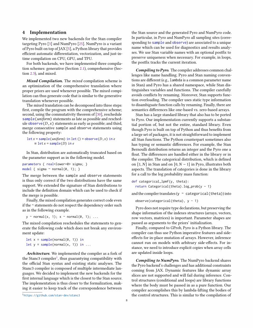
Most of themodels yield posterior distributions that match

the reference. The four remaining errors are due to the fol-

lowing missing functions in our implementation of the stan-

dard library: cov_exp_quad (accel_gp and gp_regr) and ODEsolvers (lotka_volterra and one_comp_mm_elim_abs). The

mismatch (garch11) is due to a constraint that we do not

know how to compile in Pyro/NumPyro (the domain of a

parameter is constrained by the value of another one).

3https://github.com/stan-dev/performance-tests-cmdstan4The configuration interface for NUTS in Pyro and NumPyro is similar to

the CmdStanPy interface.

Table 3 shows that NUTS in Pyro is much slower than

its NumPyro counterpart on our examples. Due to the high

computational cost of running inference in Pyro (more than

100h for hmm_drive_0), we focus on the NumPyro back-

end to compare the different compilation schemes. Results

show no difference between the comprehensive compilation

scheme and the mixed version. When the generative transla-

tion is possible, the results also match except for one example

(eight_schools_noncentered) due to a parameter constraint

that is not propagated in the model (see Section 4).

As discussed in Section 4, the mixed compilation scheme

can recover the code produced by the generative translation

when possible. Table 3 shows that the extra priors intro-

duced by the translation have no impact on the accuracy

of the inference when using NUTS. However, these priors

could play a critical role for other inference schemes, e.g.,

the importance sampling algorithm.

RQ3: Speed. To compare inference speed, Table 3 reports

average runtime for Stan and NumPyro over five runs with

varying seed values. For obvious computational cost reasons,

we only report the duration of one Pyro run. As in RQ2,

iterations, warmups, chains, and thinning configurations are

given in PosteriorDB.

Table 3 shows that the runtime of DeepStan with the

NumPyro backend is competitive with Stan under all three

compilation schemes. In addition, runtime durations for the

models compiled with the mixed, comprehensive, and gener-

ative scheme are almost identical when inference succeeds.

These results indicate that the chosen compilation scheme

has negligible influence on inference speed. Moreover, as

shown in the last column, the NumPyro backend speeds up

most benchmarks compared to the highly optimized Stan

inference engine (geometric mean: 2.3x on 26 benchmarks).

Two examples (eight_schools-eight_schools_centered and

arma11) are very sensitive to random seed variations in Stan

and NumPyro (relative standard deviation std/mean > 1).

For all other examples std/mean ≤ 0.1.

Some of the benchmarks involve nested loops that are still

experimental in NumPyro (arK, dogs, dogs_log, hmm_drive_0,

hmm_example). For these example NumPyro is typically

slower that Stan. If we exclude themwe get an overall speedup

of 3.8x on 21 benchmarks.

For Table 3 we pre-compiled the models to focus on infer-

ence time. The average compilation time for our compiler

with both backends was 0.3s (std: 0.02) compared to 10.5s (std:

5.1) for Stan. The NumPyro backend thus outperforms Stan

in both compilation and inference speed for these examples.

6.2 Stan ExtensionsThis section evaluates DeepStan, our extension with explicit

variational guides and support for deep probabilistic pro-

gramming with neural networks. We consider two questions:

11

Table 3. Comparing inference results with PosteriorDB references

Pyro NumPyro

Model Dataset Stan Compr. Compr. Mixed Gener. Speedup

accel_gp mcycle_gp ✓ 00:18:22 ✗ ✗ ✗ ✗

arK arK ✓ 00:00:57 ✓ 45:39:30 ✓ 00:00:38 ✓ 00:00:37 ✓ 00:00:34 1.48

arma11 arma ✓ 00:01:36 ✓ 02:19:07 ✓ 00:00:42 ✓ 00:21:46 ✓ 00:18:53 2.26

dogs dogs ✓ 00:01:06 ✓ 29:12:04 ✓ 00:06:22 ✓ 00:06:12 ✓ 00:06:09 0.17

dogs_log dogs ✓ 00:00:32 ✓ 23:56:20 ✓ 00:03:43 ✓ 00:03:34 ✗ 0.14

earn_height earnings ✓ 00:01:18 ✓ 01:07:03 ✓ 00:00:15 ✓ 00:00:15 ✗ 5.04

eight_schools_centered eight_schools ✓ 00:00:05 ✓ 00:27:09 ✓ 00:00:07 ✓ 00:00:06 ✓ 00:00:06 0.69

eight_schools_noncentered eight_schools ✓ 00:00:01 ✓ 00:17:36 ✓ 00:00:06 ✓ 00:00:06 ❍ 00:00:06 0.19

garch11 garch ✓ 00:00:17 ❍ 20:20:05 ❍ 00:02:07 ❍ 00:02:04 ✗

gp_regr gp_pois_regr ✓ 00:00:02 ✗ ✗ ✗ ✗

hmm_drive_0 bball_drive_event_0 ✓ 00:03:50 ✓ 108:34:15 ✓ 00:25:42 ✓ 00:25:38 ✗ 0.15

hmm_example hmm_example ✓ 00:00:28 ✓ 08:57:44 ✓ 00:01:02 ✓ 00:01:02 ✗ 0.46

kidscore_interaction kidiq ✓ 00:01:42 ✓ 01:40:32 ✓ 00:00:13 ✓ 00:00:13 ✗ 7.80

kidscore_interaction_c2 kidiq_with_mom_work ✓ 00:00:10 ✓ 00:08:58 ✓ 00:00:06 ✓ 00:00:06 ✗ 1.62

kidscore_mom_work kidiq_with_mom_work ✓ 00:00:14 ✓ 00:12:16 ✓ 00:00:09 ✓ 00:00:09 ✗ 1.66

kidscore_momhs kidiq ✓ 00:00:05 ✓ 00:12:05 ✓ 00:00:06 ✓ 00:00:06 ✗ 0.86

kidscore_momhsiq kidiq ✓ 00:00:28 ✓ 00:42:54 ✓ 00:00:08 ✓ 00:00:08 ✗ 3.32

kidscore_momiq kidiq ✓ 00:00:13 ✓ 00:30:28 ✓ 00:00:07 ✓ 00:00:07 ✗ 1.82

kilpisjarvi kilpisjarvi_mod ✓ 00:00:59 ✓ 12:12:26 ✓ 00:00:21 ✓ 00:00:21 ✗ 2.87

logearn_height earnings ✓ 00:01:19 ✓ 00:59:53 ✓ 00:00:15 ✓ 00:00:15 ✗ 5.29

logearn_height_male earnings ✓ 00:03:45 ✓ 01:36:57 ✓ 00:00:23 ✓ 00:00:23 ✗ 9.81

logearn_logheight_male earnings ✓ 00:14:27 ✓ 06:19:24 ✓ 00:01:15 ✓ 00:01:15 ✗ 11.59

logmesquite_logvas mesquite ✓ 00:00:14 ✓ 00:52:51 ✓ 00:00:08 ✓ 00:00:08 ✗ 1.84

lotka_volterra hudson_lynx_hare ✓ 00:03:06 ✗ ✗ ✗ ✗

mesquite mesquite ✓ 00:00:15 ✓ 00:59:55 ✓ 00:00:08 ✓ 00:00:08 ✗ 1.90

nes nes1980 ✓ 00:03:36 ✓ 00:50:02 ✓ 00:00:15 ✓ 00:00:15 ✗ 14.02

nes nes1976 ✓ 00:06:59 ✓ 00:54:46 ✓ 00:00:20 ✓ 00:00:21 ✗ 20.56

nes nes1972 ✓ 00:07:58 ✓ 00:50:51 ✓ 00:00:25 ✓ 00:00:25 ✗ 19.07

nes nes2000 ✓ 00:02:41 ✓ 00:56:39 ✓ 00:00:13 ✓ 00:00:13 ✗ 12.14

nes nes1996 ✓ 00:06:38 ✓ 00:55:58 ✓ 00:00:22 ✓ 00:00:22 ✗ 18.35

one_comp_mm_elim_abs one_comp_mm_elim_abs ✓ 00:16:10 ✗ ✗ ✗ ✗

✓ match, ❍ mismatch, ✗ error. Durations are reported in hh:mm:ss format. Speedup = Stan / NumPyro Compr.

RQ4: Are explicit variational guides useful?RQ5: For deep probabilistic models, how does DeepStan

compare to hand-written Pyro code?

RQ4: Explicit guides. The multimodal example shown

in Figure 10 is a mixture of two Gaussian distributions with

different means but identical variances. The first two his-

tograms of Figure 10 show that in both Stan and DeepStan,

this example is particularly challenging for NUTS. Using

multiple chains, NUTS finds the two modes, but the chains

do not mix and the relative densities are incorrect. This is a

known limitation of HMC.5

Stan also offers ADVI [19], an implementation of black-

box VI where guides are automatically synthesized from

the model using a mean-field approximation. This choice

implies that ADVI cannot approximate multi-modal distribu-

tion as illustrated in the last histogram of Figure 10. On the

5https://mc-stan.org/users/documentation/case-studies/identifying_mixture_models.html

other hand, using the custom variational guide presented in

Figure 10, DeepStan with VI is able to find the two modes.

RQ5: Deep probabilistic models. As Stan lacks support

for deep probabilistic models, it cannot be used as a base-

line. Instead, we compare the performance of the compiled

code with hand-written Pyro code on the VAE described in

Section 5.2 and a simple Bayesian neural network.

Variational autoencoders were not designed as a predic-

tive model but as a generative model to reconstruct images.

Evaluating the performance of a VAE is thus non-obvious.

We trained two VAEs on the MNIST dataset using VI: one

hand-written in Pyro, the other written in DeepStan. For

each image in the test set, the trained VAEs compute a latent

representation of dimension 5. We cluster these represen-

tations using KMeans with 10 clusters. We measure VAE

performance with the pairwise F1 metric: true positives are

the number of images of the same digit that appear in the

same cluster. For Pyro F1=0.41 (precision=0.43, recall=0.40),

12

Compiling Stan to Generative Probabilistic Languages and Extension to Deep Probabilistic Programming

parameters {real cluster; real theta; }

model {real mu;cluster ~ normal(0, 1);if (cluster > 0) mu = 20;else mu = 0;theta ~ normal(mu, 1); }

guide parameters {real m1; real m2;real<lower=0> s1;real<lower=0> s2; }

guide {cluster ~ normal(0, 1);if (cluster > 0) theta ~ normal(m1, s1);else theta ~ normal(m2, s2); }

0 10 20θ

0

500

1000 Stan(NUTS)

DeepStan(VI)

0 10 20θ

0

500

1000 DeepStan(NUTS)

DeepStan(VI)

0 10 20θ

0

500

1000 DeepStan(VI)

Stan(ADVI)

Figure 10. DeepStan code and histograms of the multimodal

example using Stan, DeepStan with NUTS, DeepStan with

VI, and Stan with ADVI.

and for DeepStan F1=0.43 (precision=0.44, recall=0.42). These

numbers shows that compiling DeepStan to Pyro does not

impact the performance of such deep probabilistic models.

We trained two implementations of a 2-level Bayesian

multi-layer perceptron (MLP) with the parameters all lifted

to random variables (see section 5.3): one hand-written in

Pyro, the other written in DeepStan. We trained both models

for 20 epochs on the training set. For each model we gener-

ated 100 samples of concrete weights and biases to obtain

an ensemble MLP that can be used to compute a distribution

of predicted labels. The accuracy for both models is 92% on

the test set and the agreement between the two models is

above 95%. The execution time is comparable. These exper-

iments show that compiling DeepStan models to Pyro has

little impact on the model. Changing the priors on the net-

work parameters from normal(0,1) to normal(0,10) (seeSection 5.3) increases accuracy from 0.92 to 0.96. This fur-

ther validates our compilation, compiling parameter priors

to observe statements on deep probabilistic models.

7 Related workTo the best of our knowledge, we propose the first compre-

hensive translation of Stan to a generative PPL. The closest

related work was developed by the Pyro team [8]. Their

work focuses on performance and ours on completeness.

Their proposed compilation technique corresponds to the

generative translation presented in Section 2.1 and thus only

handles a subset of Stan. The code is not open-source, and

we rely on our own implementation of the generative trans-

lation in Section 6. Compared to our approach, they are also

looking into independence assumptions between loop itera-

tions to generate parallel code. Combining these ideas with

our approach is a promising future direction. They do not

extend Stan with either VI or neural networks. Similarly, in

Appendix B.2 of [15], Gorinova et al. outline the generative

translation of Section 2.1, and also mention the issue with

multiple updates but do not provide a solution. Lee et al.

[20] introduce a density-based semantics for Pyro, but this

semantics does not handle Stan’s non-generative features.

The goal of compiling Stan to Pyro is to create a platform

for experimenting with new ideas. For example, Section 5.1

extends Stan with explicit variational guides. Similarly, Pyro

now offers inference on discrete parameters6that we could

port to Stan using our backends.

In recent years, taking advantage of the maturity of DL

frameworks, multiple deep probabilistic programming lan-

guages have been proposed: PyMC3 [28] built on top of

Theano, Edward [33] and ZhuSuan [29] built on top of Ten-

sorFlow, and Pyro [3] and ProbTorch [22] built on top of

PyTorch. All these languages are implemented as libraries.

The users thus need to master the entire technology stack

of the library, the underlying DL framework, and the host

language. In comparison, DeepStan is a self-contained lan-

guage and the compiler helps the programmer via dedicated

static analyses.

8 ConclusionThis paper introduces a comprehensive compilation scheme

from Stan to generative probabilistic programming languages.

This shows that Stan is at most as expressive as this family

of languages. We implemented a compiler from Stan to Pyro.

Additionally, we designed and implemented extensions for

Stan with explicit variational guides and neural networks.

Acknowledgement. The authors are greatful to the fol-

lowing people for their helpful feedback and encouragements

during this work: E. Bingham, K. Kate, Y. Mroueh, F. Ober-

meyer, and A. Pauthier.

References[1] Guillaume Baudart, Javier Burroni, Martin Hirzel, Louis Mandel, and

Avraham Shinnar. 2021. Compiling Stan to Generative Probabilistic

Languages and Extension to Deep Probabilistic Programming. In PLDI.ACM.

[2] Guillaume Baudart, Martin Hirzel, and Louis Mandel. 2018. Deep

Probabilistic Programming Languages: A Qualitative Study. CoRRabs/1804.06458 (2018).

[3] Eli Bingham, Jonathan P. Chen, Martin Jankowiak, Fritz Obermeyer,

Neeraj Pradhan, Theofanis Karaletsos, Rohit Singh, Paul A. Szerlip,

Paul Horsfall, and Noah D. Goodman. 2019. Pyro: Deep Universal

Probabilistic Programming. J. Mach. Learn. Res. 20 (2019), 28:1–28:6.[4] David M. Blei, Alp Kucukelbir, and Jon D. McAuliffe. 2016. Variational

Inference: A Review for Statisticians. CoRR abs/1601.00670 (2016).

[5] James Bradbury, Roy Frostig, Peter Hawkins, Matthew James Johnson,

Chris Leary, Dougal Maclaurin, and Skye Wanderman-Milne. 2018.

JAX: composable transformations of Python+NumPy programs. http://github.com/google/jax

[6] Bradley P Carlin and Thomas A Louis. 2008. Bayesian methods for dataanalysis. CRC Press.

6https://pyro.ai/examples/enumeration.html

13

[7] Bob Carpenter, Andrew Gelman, Matthew D Hoffman, Daniel Lee,

Ben Goodrich, Michael Betancourt, Marcus Brubaker, Jiqiang Guo,

Peter Li, and Allen Riddell. 2017. Stan: A probabilistic programming

language. Journal of Statistical Software 76, 1 (2017), 1–37. https://doi.org/10.18637/jss.v076.i01

[8] Jonathan P. Chen, Rohit Singh, Eli Bingham, and Noah Goodman. 2018.

Transpiling Stan models to Pyro. In ProbProg.[9] Marco F. Cusumano-Towner, Feras A. Saad, Alexander K. Lew, and

Vikash K. Mansinghka. 2019. Gen: a general-purpose probabilistic

programming system with programmable inference. In PLDI. ACM,

221–236. https://doi.org/10.1145/3314221.3314642[10] Andrew Gelman and Jennifer Hill. 2006. Data analysis using regression

andmultilevel/hierarchical models. Cambridge university press. https://doi.org/10.1017/CBO9780511790942

[11] Andrew Gelman, Hal S Stern, John B Carlin, David B Dunson, Aki

Vehtari, and Donald B Rubin. 2013. Bayesian data analysis. Chapman

and Hall/CRC.

[12] Noah D. Goodman, Vikash K. Mansinghka, Daniel M. Roy, Keith

Bonawitz, and Joshua B. Tenenbaum. 2008. Church: a language for

generative models. In UAI. AUAI Press, 220–229.[13] Noah D. Goodman and Andreas Stuhlmüller. 2014. The Design and

Implementation of Probabilistic Programming Languages. http://dippl.org Accessed April 2021.

[14] Andrew D. Gordon, Thomas A. Henzinger, Aditya V. Nori, and Sri-

ram K. Rajamani. 2014. Probabilistic programming. In FOSE. ACM,

167–181. https://doi.org/10.1145/2593882.2593900[15] Maria I. Gorinova, Andrew D. Gordon, and Charles Sutton. 2019. Prob-

abilistic programming with densities in SlicStan: efficient, flexible, and

deterministic. Proc. ACM Program. Lang. 3, POPL (2019), 35:1–35:30.

https://doi.org/10.1145/3290348[16] Matthew D. Hoffman and Andrew Gelman. 2014. The No-U-turn

sampler: adaptively setting path lengths in Hamiltonian Monte Carlo.

J. Mach. Learn. Res. 15, 1 (2014), 1593–1623.[17] Diederik P. Kingma andMaxWelling. 2014. Auto-Encoding Variational

Bayes. In ICLR.[18] Dexter Kozen. 1981. Semantics of Probabilistic Programs. J. Comput.

Syst. Sci. 22, 3 (1981), 328–350. https://doi.org/10.1016/0022-0000(81)90036-2

[19] Alp Kucukelbir, Dustin Tran, Rajesh Ranganath, Andrew Gelman, and

David M. Blei. 2017. Automatic Differentiation Variational Inference.

J. Mach. Learn. Res. 18 (2017), 14:1–14:45.[20] Wonyeol Lee, Hangyeol Yu, Xavier Rival, and Hongseok Yang. 2020.

Towards verified stochastic variational inference for probabilistic pro-

grams. PACMPL 4, POPL (2020), 16:1–16:33. https://doi.org/10.1145/3371084

[21] David Lunn, David Spiegelhalter, Andrew Thomas, and Nicky Best.

2009. The BUGS project: Evolution, critique and future directions. Stat.

in medicine 28, 25 (2009), 3049–3067. https://doi.org/10.1002/sim.3680

[22] Siddharth Narayanaswamy, Brooks Paige, Jan-Willem van de Meent,

Alban Desmaison, Noah D. Goodman, Pushmeet Kohli, Frank D. Wood,

and Philip H. S. Torr. 2017. Learning Disentangled Representations

with Semi-Supervised Deep Generative Models. In NIPS. 5925–5935.[23] Radford M. Neal. 1996. Bayesian Learning for Neural Networks. Vol. 118.

Springer. https://doi.org/10.1007/978-1-4612-0745-0[24] Adam Paszke, Sam Gross, Soumith Chintala, Gregory Chanan, Edward

Yang, Zachary DeVito, Zeming Lin, AlbanDesmaison, Luca Antiga, and

Adam Lerer. 2017. Automatic Differentiation in PyTorch. In AutoDiffWorkshop.

[25] Du Phan, Neeraj Pradhan, and Martin Jankowiak. 2019. Composable

Effects for Flexible and Accelerated Probabilistic Programming in

NumPyro. CoRR abs/1912.11554 (2019).

[26] Martyn Plummer et al. 2003. JAGS: A program for analysis of Bayesian

graphical models using Gibbs sampling. In Workshop on distr. stat.comp., Vol. 124. Vienna, Austria.

[27] Danilo Jimenez Rezende, Shakir Mohamed, and Daan Wierstra. 2014.

Stochastic Backpropagation and Approximate Inference in Deep Gen-

erative Models. In ICML (JMLR Workshop and Conference Proceedings,Vol. 32). JMLR.org, 1278–1286.

[28] John Salvatier, Thomas V. Wiecki, and Christopher Fonnesbeck. 2016.

Probabilistic programming in Python using PyMC3. PeerJ Comput. Sci.2 (2016), e55. https://doi.org/10.7717/peerj-cs.55

[29] Jiaxin Shi, Jianfei Chen, Jun Zhu, Shengyang Sun, Yucen Luo, Yihong

Gu, and Yuhao Zhou. 2017. ZhuSuan: A Library for Bayesian Deep

Learning. CoRR abs/1709.05870 (2017).

[30] Sam Staton. 2017. Commutative Semantics for Probabilistic Program-

ming. In ESOP (Lecture Notes in Computer Science, Vol. 10201). Springer,855–879. https://doi.org/10.1007/978-3-662-54434-1_32

[31] Sam Staton, Hongseok Yang, Frank D. Wood, Chris Heunen, and Ohad

Kammar. 2016. Semantics for probabilistic programming: higher-order

functions, continuous distributions, and soft constraints. In LICS. ACM,

525–534. https://doi.org/10.1145/2933575.2935313[32] David Tolpin, Jan-Willem van de Meent, Hongseok Yang, and Frank D.

Wood. 2016. Design and Implementation of Probabilistic Programming

Language Anglican. In IFL. ACM, 6:1–6:12. https://doi.org/10.1145/3064899.3064910

[33] Dustin Tran, Matthew D. Hoffman, Rif A. Saurous, Eugene Brevdo,

Kevin Murphy, and David M. Blei. 2017. Deep Probabilistic Program-

ming. In ICLR (Poster).[34] Jan-Willem van de Meent, Brooks Paige, Hongseok Yang, and Frank

Wood. 2018. An Introduction to Probabilistic Programming. CoRRabs/1809.10756 (2018).

[35] Aki Vehtari and Måns Magnusson. 2020. PosteriorDB: a database with

data, models and posteriors. In Stan Conf. https://github.com/stan-dev/posteriordb

14

Compiling Stan to Generative Probabilistic Languages and Extension to Deep Probabilistic Programming

A Auxiliary LemmasThe first additional property that we need is that the initial

value of target only impact the final value of target but

no other variable.

Lemma A.1. For all Stan statement stmt, for all variable 𝑥different from target, then for all values 𝑡1 and 𝑡2,

JstmtK𝛾 [target←𝑡1 ] (𝑥) = JstmtK𝛾 [target←𝑡2 ] (𝑥)

Proof. The proof is done by induction on the structure of

the statements and number of reductions. We detail just the

most interesting cases.

Assignment. Evaluating 𝑥 = 𝑒 does not update targetand according to Assumption 2, the expression 𝑒 does not de-

pends on the value of target. So J𝑒K𝛾 [target←𝑡1 ] = J𝑒K𝛾 [target←𝑡2 ]and thus J𝑥 = 𝑒K𝛾 [target←𝑡1 ] (𝑥) = J𝑥 = 𝑒K𝛾 [target←𝑡2 ] (𝑥).

Target Update. Since the evaluation of target += 𝑒 onlyupdates the value of target, we have by definition

Jtarget += 𝑒K𝛾 [target←𝑡1 ] (𝑥) = Jtarget += 𝑒K𝛾 [target←𝑡2 ] (𝑥)

Sequence. For a sequence stmt1; stmt2 we have:

Jstmt1; stmt2K𝛾 [target←𝑡1 ] (𝑥)= Jstmt2KJstmt1K𝛾 [target←𝑡

1](𝑥) { by definition }

= Jstmt2KJstmt1K𝛾 [target←𝑡2](𝑥) { by induction on stmt1 }

= Jstmt1; stmt2K𝛾 [target←𝑡2 ] (𝑥) { by definition }

Loop. For a loop while (𝑒) {𝑠}, by induction on the struc-

ture of the statements, for all environment 𝛾 , values 𝑡1 and

𝑡2 and variable 𝑥 ≠ target, we have J𝑠K𝛾 [target←𝑡1 ] (𝑥) =J𝑠K𝛾 [target←𝑡2 ] (𝑥), which implies:

J𝑠K𝛾 [target←𝑡1 ] = J𝑠K𝛾 [target← J𝑠K𝛾 [target←𝑡1 ] ]

In addition, by Assumption 2 we know that for all envi-

ronment 𝛾 , J𝑒K𝛾 [target←𝑡1 ] = J𝑒K𝛾 [target←𝑡2 ] .By Assumption 1, there is a finite number 𝑛 of loop it-

erations. So we can prove by induction on the number of

remaining iterations that for all 𝑡1, 𝑡2:

Jwhile (𝑒) {𝑠}K𝛾𝑛 [target←𝑡1 ] (𝑥) = Jwhile (𝑒) {𝑠}K𝛾𝑛 [target←𝑡2 ] (𝑥)

where for all 0 ≤ 𝑖 < 𝑛, 𝛾𝑖 = J𝑠K𝛾𝑖+1 , and 𝛾𝑛 = 𝛾 .

If 𝑛 = 0, J𝑒K𝛾0 [target←𝑡1 ] = J𝑒K𝛾0 [target←𝑡2 ] = 0. So by

definition of the semantics we have:

𝛾0 [target← 𝑡1] (𝑥) = 𝛾0 [target← 𝑡2] (𝑥)

For the inductive case, if 𝑛 = 𝑖 + 1, there are some itera-

tions left so J𝑒K𝛾𝑖+1 [target←𝑡1 ] = J𝑒K𝛾𝑖+1 [target←𝑡2 ] ≠ 0. So by

definition of the semantics we have:

Jwhile (𝑒) {𝑠}K𝛾𝑖+1 [target←𝑡1 ] (𝑥)= Jwhile (𝑒) {𝑠}KJ𝑠K

𝛾𝑖+1 [target←𝑡1](𝑥) { by definition }

= { by definition of 𝛾𝑖 and induction on 𝑠 }Jwhile (𝑒) {𝑠}K𝛾𝑖 [target←J𝑠K

𝛾𝑖+1 [target←𝑡1] (target) ] (𝑥)

= Jwhile (𝑒) {𝑠}K𝛾𝑖 [target←𝑡2 ] (𝑥) { induction on 𝑠 }= { by definition of 𝛾𝑖 and induction on 𝑠 }

Jwhile (𝑒) {𝑠}KJ𝑠K𝛾𝑖+1 [target←𝑡2 ] (𝑥)

= Jwhile (𝑒) {𝑠}K𝛾𝑖+1 [target←𝑡2 ] (𝑥) { by definition }□

The next lemma state that every statement can be evalu-

ated in an environment where target is set to zero.

LemmaA.2. For all Stan statement stmt and any real value 𝑡we have:

JstmtK𝛾 [target←𝑡 ] (target) = 𝑡+JstmtK𝛾 [target←0] (target)

Proof. The proof is done by induction on the structure of the

statements and number of reductions.

Assignment. Evaluating 𝑥 = 𝑒 does not update target.Therefore, for all 𝑡 , J𝑥 = 𝑒K𝛾 [target←𝑡 ] (target) = 𝑡 and thus

J𝑥 = 𝑒K𝛾 [target←𝑡 ] (target) = 𝑡+J𝑥 = 𝑒K𝛾 [target←0] (target)

Target Update. Since the evaluation of target += 𝑒 onlyupdates the value of target, we have by definition

Jtarget += 𝑒K𝛾 [target←𝑡 ] (target)= 𝑡 + Jtarget += 𝑒K𝛾 [target←0] (target)

Sequence. Let 𝛾1 = Jstmt1K𝛾 [target←0] . By induction, we

have Jstmt1K𝛾 [target←𝑡 ] = 𝑡 + 𝛾1 (target).

Jstmt1; stmt2K𝛾 [target←𝑡 ] (target)= Jstmt2KJstmt1K𝛾 [target←𝑡 ]

(target) { by definition }= { by induction on stmt2 }

Jstmt1K𝛾 [target←𝑡 ] (target)+ Jstmt2KJstmt1K𝛾 [target←𝑡 ] [target←0] (target)

= { by induction on stmt1 }𝑡 + Jstmt1K𝛾 [target←0] (target)+ Jstmt2KJstmt1K𝛾 [target←𝑡 ] [target←0] (target)

= { by Lemma A.1 and induction on stmt2 }𝑡 + Jstmt2KJstmt1K𝛾 [target←0] [target←0] (target)

= 𝑡 + Jstmt1; stmt2K𝛾 [target←0] (target) { by definition }

15

Loops. By Assumption 1, there is a finite number 𝑛 of loop

iterations. So we can prove by induction on the number of

remaining iterations that

Jwhile (𝑒) {𝑠}K𝛾𝑛 [target←𝑡 ] (target)= 𝑡 + Jwhile (𝑒) {𝑠}K𝛾𝑛 [target←0] (target)

where for all 0 ≤ 𝑖 < 𝑛, 𝛾𝑖 = J𝑠K𝛾𝑖+1 , and 𝛾𝑛 = 𝛾 .

If 𝑛 = 0, J𝑒K𝛾0 [target←𝑡 ] = J𝑒K𝛾0 [target←0] = 0. So by defi-

nition of the semantics we have:

𝛾0 [target← 𝑡] (target) = 𝑡 + 𝛾0 [target← 0] (target)

For the inductive case, if𝑛 = 𝑖+1, there are some iterations

left so by definition of the semantics we have:

Jwhile (𝑒) {𝑠}K𝛾𝑖+1 [target←𝑡 ] (target)= Jwhile (𝑒) {𝑠}KJ𝑠K

𝛾𝑖+1 [target←𝑡 ](target) { by definition }

= { by definition of 𝛾𝑖 and Lemma A.1 }Jwhile (𝑒) {𝑠}K𝛾𝑖 [target←J𝑠K

𝛾𝑖+1 [target←t] (target) ] (target)= { by induction on the number of reductions }

J𝑠K𝛾𝑖+1 [target←t] (target)+ Jwhile (𝑒) {𝑠}K𝛾𝑖 [target←0] (target)

= { by induction on 𝑠 }𝑡 + J𝑠K𝛾𝑖+1 [target←0] (target)+ Jwhile (𝑒) {𝑠}K𝛾𝑖 [target←0] (target)

= { by definition of 𝛾𝑖 }𝑡 + J𝑠K𝛾𝑖+1 [target←0] (target)+ Jwhile (𝑒) {𝑠}KJ𝑠K

𝛾𝑖+1 [target←0] (target)= { by Lemma A.1 }𝑡 + J𝑠K𝛾𝑖+1 [target←0] (target)+ Jwhile (𝑒) {𝑠}KJ𝑠K

𝛾𝑖+1 [target←0] [target←0] (target)= { by induction }𝑡 + Jwhile (𝑒) {𝑠}K𝛾𝑖+1 [target←0] (target)

□

B Proofs: Correctness of the CompilationLemma B.1. For all Stan programs 𝑝 with stmt = model(𝑝)and P = params(𝑝), and environments 𝛾 :

{[C(𝑝)]}𝛾 ∝ _𝑈 .

∫𝑈

{[Creturn(()) (stmt)]}𝛾 [P←\ ] ({()})𝑑\

Proof. Let P = 𝑥1, ..., 𝑥𝑛 . By definition of the compilation

function, C(𝑝) has the shape:let𝑥1 = 𝐷1 in . . . let𝑥𝑛 = 𝐷𝑛 in Creturn(P) (stmt)

where for each parameter 𝑥𝑖 , the distribution 𝐷𝑖 is either

uniform or improper_uniform. In both cases the correspond-ing density is constant w.r.t. the Lebesgue measure on its

domain.

Since the kernels defined by GProb expressions are always

s-finite [30], from the semantics of GProb (Section 3.2) and

the Fubini-Tonelli theorem, we have:

{[C(𝑝)]}𝛾

= {[let𝑥1 = 𝐷1 in . . . let𝑥𝑛 = 𝐷𝑛 in Creturn(P) (stmt)]}𝛾

= _𝑈 .

∫𝑋1

𝐷1 (𝑑𝑣1) ...∫𝑋𝑛𝐷𝑛 (𝑑𝑣𝑛){[Creturn(P) (stmt)]}𝛾 [ (𝑥1,...,𝑥𝑛)←(𝑣1,...,𝑣𝑛) ] (𝑈 )

∝ _𝑈 .

∫𝑋1

...

∫𝑋𝑛

{[Creturn(P) (stmt)]}𝛾 [ (𝑥1,...,𝑥𝑛)←(𝑣1,...,𝑣𝑛) ] (𝑈 ) 𝑑𝑣1 ...𝑑𝑣𝑛

= _𝑈 .

∫𝑋=𝑋1×...×𝑋𝑛

{[Creturn(P) (stmt)]}𝛾 [ (𝑥1,...,𝑥𝑛)←\ ] (𝑈 ) 𝑑\

The evaluation of {[Creturn(P) (stmt)]}𝛾 [P←\ ] (𝑈 ) termi-

nates with the value {[return(P)]}𝛾 ′ [P←\ ] (𝑈 ) where 𝛾 ′ isthe environment obtained after the evaluation of the model

statements stmt.However, in Stan, parameters declared in P cannot appear

in the left-hand side of an assignment. The evaluation of the

model statements stmt cannot update the value of the param-

eters. We can thus simplify {[return(P)]}𝛾 ′ [P←\ ] (𝑈 ) into{[return(P)]} [P←\ ] (𝑈 ). The evaluation of the compiled

code can then be decomposed as follows:

{[Creturn(P) (stmt)]}𝛾 [P←\ ] (𝑈 )

=

∫𝑋

{[Creturn(()) (stmt)]}𝛾 [P←\ ] (𝑑𝑥) ×{[return(P)]} [P←\ ] (𝑈 )

= {[Creturn(()) (stmt)]}𝛾 [P←\ ] ({()}) × 𝛿\ (𝑈 )

Going back to the previous equation, we now have

{[C(𝑝)]}𝛾

= _𝑈 .

∫𝑋

{[Creturn(()) (stmt)]}𝛾 [P←\ ] ({()}) × 𝛿\ (𝑈 ) 𝑑\

= _𝑈 .

∫𝑈

{[Creturn(()) (stmt)]}𝛾 [P←\ ] ({()}) 𝑑\

□

Lemma B.2. For all Stan statements stmt compiled with acontinuation 𝑘 , if 𝛾 (target) = 0, and JstmtK𝛾 = 𝛾 ′,

{[C𝑘 (stmt)]}𝛾 = _𝑈 . exp(𝛾 ′(target)) ×{[𝑘]}𝛾 ′ [target←0] (𝑈 )

Proof. The proof is done by induction on the structure of stmtand number of reductions using the definition of the compi-

lation function (Section 3.3) and the semantics of GProb.

Assignment. Evaluating 𝑥 = 𝑒 does not update targetand its initial value is 0 by hypothesis. With 𝛾 ′ = J𝑥 = 𝑒K𝛾 wehave 𝛾 ′[target← 0] = 𝛾 ′ and exp(𝛾 ′(target)) = 1. Then

from GProb’s semantics we have:

16

Compiling Stan to Generative Probabilistic Languages and Extension to Deep Probabilistic Programming

{[C𝑘 (𝑥 = 𝑒)]}𝛾 = { by definition of C𝑘 (.) }{[let𝑥 = return(𝑒) in 𝑘]}𝛾

= { by definition of the semantics }

_𝑈 .

∫𝑋

{[return(𝑒)]}𝛾 (𝑑𝑣) × {[𝑘]}𝛾 [𝑥←𝑣 ] (𝑈 )

= { by definition of the semantics }

_𝑈 .

∫𝑋

𝛿J𝑒K𝛾 (𝑑𝑣) × {[𝑘]}𝛾 [𝑥←𝑣 ] (𝑈 )

= { by the integration of the 𝛿 distribution }_𝑈 .1 × {[𝑘]}𝛾 [𝑥←J𝑒K𝛾 ] (𝑈 )

= { by the semantics of J𝑥 = 𝑒K𝛾 }_𝑈 .1 × {[𝑘]}J𝑥 = 𝑒K𝛾 (𝑈 )

= { by definition of 𝛾 ′ }_𝑈 . exp(𝛾 ′(target)) × {[𝑘]}𝛾 ′ [target←0] (𝑈 )

Target update. Since the evaluation of target += 𝑒 onlyupdates the value of target and its initial value is 0, with

𝛾 ′ = Jtarget += 𝑒K𝛾 we have 𝛾 = 𝛾 ′[target ← 0], and𝛾 ′(target) = J𝑒K𝛾 . Then from GProb’s semantics we have:

{[C𝑘 (target += 𝑒)]}𝛾= { by definition of C𝑘 (.) }{[let () = factor(𝑒) in 𝑘]}𝛾

= { by definition of the semantics }

_𝑈 .

∫()

exp(J𝑒K𝛾 )𝛿() (𝑑𝑣) × {[𝑘]}𝛾 (𝑈 )

= { by the integration of the 𝛿 distribution }_𝑈 . exp(J𝑒K𝛾 ) × {[𝑘]}𝛾 (𝑈 )

= { by the semantics of Jtarget += 𝑒K𝛾 }_𝑈 . exp(Jtarget += 𝑒K𝛾 (target)) × {[𝑘]}𝛾 (𝑈 )

= { by definition of 𝛾 ′ }_𝑈 . exp(𝛾 ′(target)) × {[𝑘]}𝛾 ′ [target←0] (𝑈 )

Sequence. If 𝛾1 = Jstmt1K𝛾 and 𝛾2 = Jstmt2K𝛾1 [target←0] ,the induction hypothesis and the semantics of GProb yield:

{[C𝑘 (stmt1; stmt2)]}𝛾 = {[CC𝑘 (stmt2) (stmt1)]}𝛾= { by induction on stmt1 and definition of 𝛾1 }_𝑈 .exp(𝛾1 (target)) × {[C𝑘 (stmt2)]}𝛾1 [target←0] (𝑈 )

= { by induction on stmt2 and definition of 𝛾2 }_𝑈 .exp(𝛾1 (target)) × exp(𝛾2 (target)) × {[𝑘]}𝛾2 [target←0] (𝑈 )

= _𝑈 .exp(𝛾1 (target) + 𝛾2 (target)) × {[𝑘]}𝛾2 [target←0] (𝑈 )

On the other hand, from Lemma A.2 we have:

Jstmt1; stmt2K𝛾 (target) = 𝛾1 (target)+𝛾2 (target) whichconclude the proof of this case.

Loop. For the case while (𝑒) {𝑠}, we first look at the

semantics of the loop on the Stan side. We can prove that

Jwhile (𝑒) {𝑠}K𝛾 (target) =𝑛−1∑︁𝑖=0

𝛾𝑖 (target) (1)

where 𝑛 is the number of loop iterations, for all 0 ≤ 𝑖 < 𝑛,

𝛾𝑖 = J𝑠K𝛾𝑖+1 [target←0] , and 𝛾𝑛 = 𝛾 . By Assumption 1 the

programs terminate, so 𝑛 is finite.

This is a direct consequence of the following property

since 𝛾 (target) = 0:

Jwhile (𝑒) {𝑠}K𝛾𝑛 [target←0] (target) =𝑛−1∑︁𝑖=0

𝛾𝑖 (target) (2)

The proof of eq. (2) is done by induction on the number

of remaining iterations. If 𝑛 = 0, the condition of the loop is

false. Since the condition of the loop cannot depend on the

value of target, it means that J𝑒K𝛾0 = J𝑒K𝛾0 [target←0] = 0,

so by application of the semantics we have directly:

Jwhile (𝑒) {𝑠}K𝛾0 [target←0] (target) = 0

For the inductive case (𝑛 = 𝑖 + 1), there is some loop

iterations remaining and thus J𝑒K𝛾𝑖+1 = J𝑒K𝛾𝑖+1 [target←0] ≠ 0.

By application on the semantics we have:

Jwhile (𝑒) {𝑠}K𝛾𝑖+1 [target←0] (target)= Jwhile (𝑒) {𝑠}KJ𝑠K

𝛾𝑖+1 [target←0]

= Jwhile (𝑒) {𝑠}K𝛾𝑖 { by definition of 𝛾𝑖 }= 𝛾𝑖 + Jwhile (𝑒) {𝑠}K𝛾𝑖 [target←0] { by Lemma A.2 }= { by induction on the number of iterations }

𝛾𝑖 +𝑖−1∑︁𝑗=0

𝛾 𝑗 (target) =𝑖∑︁𝑗=0

𝛾 𝑗 (target)

Let’s look at the loop whileX (𝑒) Creturn(X) (𝑠) where Xis the variables updated by 𝑠 (lhs(𝑠) = X). We will use the

two following properties. For all 𝛾 , if J𝑒K𝛾 = 0

{[whileX (𝑒) Creturn(X) (𝑠)]}𝛾 = 𝛿𝛾 (X) (3)

For all 𝛾 , if J𝑒K𝛾 ≠ 0 and J𝑠K𝛾 = 𝛾 ′:

{[whileX (𝑒) Creturn(X) (𝑠)]}𝛾= _𝑈 .exp(𝛾 ′(target)) ×

{[whileX (𝑒) Creturn(X) (𝑠)]}𝛾 ′ [target←0] (𝑈 )(4)

The proofs of both of these properties start by unfolding the

definition of the semantics:

{[whileX (𝑒) Creturn(X) (𝑠)]}𝛾= _𝑈 .if J𝑒K𝛾 = 0 then 𝛿𝛾 (X) (𝑈 )

else∫𝑋

{[Creturn(X) (𝑠)]}𝛾 (𝑑𝑣) ×{[whileX (𝑒) Creturn(X) (𝑠)]}𝛾 [X←𝑣 ] (𝑈 )

From there, the proof of eq. (3) where J𝑒K𝛾 = 0 is trivial. For

eq. (4) where J𝑒K𝛾 ≠ 0 and J𝑠K𝛾 = 𝛾 ′, we apply the induction

17

hypothesis on {[Creturn(X) (𝑠)]}𝛾 :

{[whileX (𝑒) Creturn(X) (𝑠)]}𝛾= { by simplification of J𝑒K𝛾 ≠ 0}

_𝑈 .

∫𝑋

{[Creturn(X) (𝑠)]}𝛾 (𝑑𝑣) ×{[whileX (𝑒) Creturn(X) (𝑠)]}𝛾 [X←𝑣 ] (𝑈 )

= { by induction on the structure of the statement}

_𝑈 .

∫𝑋

(exp(𝛾 ′(target)) × {[return(X)]}𝛾 ′ [target←0] ) (𝑑𝑣) ×{[whileX (𝑒) Creturn(X) (𝑠)]}𝛾 [X←𝑣 ] (𝑈 )

= { by definition of the semantics of return}

_𝑈 .

∫𝑋

(exp(𝛾 ′(target)) × 𝛿𝛾 ′ [target←0] (X) ) (𝑑𝑣) ×{[whileX (𝑒) Creturn(X) (𝑠)]}𝛾 [X←𝑣 ] (𝑈 )

= { by the integration of the 𝛿 distribution }_𝑈 .exp(𝛾 ′(target)) ×{[whileX (𝑒) Creturn(X) (𝑠)]}𝛾 [X←𝛾 ′ [target←0] (X) ] (𝑈 )

= { the only difference between 𝛾 and 𝛾 ′ are in X by def of lhs }_𝑈 .exp(𝛾 ′(target)) ×{[whileX (𝑒) Creturn(X) (𝑠)]}𝛾 ′ [target←0] (𝑈 )

We can now prove by induction on the number of loop

iterations 𝑛 (that we assume finite) that

{[whileX (𝑒) Creturn(X) (𝑠)]}𝛾𝑛 [target←0]

= _𝑈 .

(𝑛−1∏𝑖=0

exp(𝛾𝑖 (target)))× 𝛿𝛾0 (X) (𝑈 )

(5)

where for all 0 ≤ 𝑖 < 𝑛, 𝛾𝑖 = J𝑠K𝛾𝑖+1 [target←0] .In the base case of the induction (𝑛 = 0), there is nomore it-

eration (J𝑒K𝛾0 = J𝑒K𝛾0 [target←0] = 0). By application of eq. (3),

we have:

{[whileX (𝑒) Creturn(X) (𝑠)]}𝛾0 [target←0] = 𝛿𝛾 (X)

For the inductive case (𝑛 = 𝑖 + 1), we know that J𝑒K𝛾𝑖+1 =J𝑒K𝛾𝑖+1 [target←0] ≠ 0 since there are some more loop itera-

tions to execute. Therefore, we can apply eq. (4):

{[whileX (𝑒) Creturn(X) (𝑠)]}𝛾𝑖+1 [target←0]

= { by eq. (4) and definition of 𝛾𝑖 }_𝑈 .exp(𝛾𝑖 (target)) ×{[whileX (𝑒) Creturn(X) (𝑠)]}𝛾𝑖 [target←0] (𝑈 )

= { by induction on the number of iterations }

_𝑈 .exp(𝛾𝑖 (target)) × ©­«𝑖−1∏𝑗=0

exp(𝛾 𝑗 (target))ª®¬ × 𝛿𝛾0 (X) (𝑈 )

= _𝑈 .©­«

𝑖∏𝑗=0

exp(𝛾 𝑗 (target))ª®¬ × 𝛿𝛾0 (X) (𝑈 )

We can finally put all the pieces together to prove the

case of while (𝑒) {𝑠}. We still assume that the loop has

𝑛 iterations. We first unroll the definition of compilation

function and the semantics.

{[C𝑘 (while (𝑒) {𝑠})]}𝛾= {[letX = whileX (𝑒) Creturn(X) (𝑠) in 𝑘]}𝛾= _𝑈 .

∫𝑋

{[whileX (𝑒) Creturn(X) (𝑠)]}𝛾 (𝑑𝑣) × {[𝑘]}𝛾 [X←𝑣 ] (𝑈 )

= { by eq. (5) with 𝛾𝑛 = 𝛾 and because 𝛾 (target) = 0 }

_𝑈 .

∫𝑋

(𝑛−1∏𝑖=0

exp(𝛾𝑖 (target)))× 𝛿𝛾0 (X) (𝑑𝑣) × {[𝑘]}𝛾 [X←𝑣 ] (𝑈 )

= { by rewriting the product of exponential }

_𝑈 .

∫𝑋

exp(𝑛−1∑︁𝑖=0

𝛾𝑖 (target)) × 𝛿𝛾0 (X) (𝑑𝑣) × {[𝑘]}𝛾 [X←𝑣 ] (𝑈 )

= { by eq. (1) with 𝛾 ′ = Jwhile (𝑒) {𝑠}K𝛾 }

_𝑈 .

∫𝑋

exp(𝛾 ′(target)) × 𝛿𝛾0 (X) (𝑑𝑣) × {[𝑘]}𝛾 [X←𝑣 ] (𝑈 )

= { by the integration of the 𝛿 distribution }_𝑈 . exp(𝛾 ′(target)) × {[𝑘]}𝛾 [X←𝛾0 (X) ] (𝑈 )

= { by definition of lhs and since target ∉ X }_𝑈 . exp(𝛾 ′(target)) × {[𝑘]}𝛾0 [target←0] (𝑈 )

= _𝑈 . exp(𝛾 ′(target)) × {[𝑘]}𝛾 ′ [target←0] (𝑈 )

□

C EvaluationWe present here the results of the experiments for RQ2 and

RQ3 described in Section 6 on the entire set of PosteriorDB

models with reference, that is, without filtering out the mod-

els for which Stan does not pass the accuracy test.

RQ2: Accuracy. Table 4 presents the accuracy results. Foreach run we report the mean relative error in green if the

model pass the accuracy test, orange otherwise (the accuracy

test fails if the relative error for one of the parameter is

above 0.3).

Compared to the results presented in Section 6 we have

two additional errors for theNumPyro backend: gp_pois_regr

(missing cov_exp_quad) and diamonds_diamonds (missing

student_t_lccdf).We also have two additional mismatches

low_dim_gauss_mix and hmm_drive_1 both due to an orderedconstraint that is not supported in the versions of Pyro and

NumPyro that we used.

For the Pyro backend two examples for which Stan returns

a mismatch timed-out after 10h (indicated with a “—” in

Table 4): hmm_drive_1 and low_dim_gauss_mix.

RQ3: Speed. Table 5 presents the speed results. For each

run we report the average duration in second and the stan-

dard deviation.

18

Compiling Stan to Generative Probabilistic Languages and Extension to Deep Probabilistic Programming

Table 4. Comparing inference results with PosteriorDB references. For each column we report the mean relative error in

green if the example pass the accuracy test, orange otherwise.

Pyro NumPyro

Model Dataset Stan Compr. Compr. Mixed Gener.

accel_gp mcycle_gp 0.01 ✗ ✗ ✗ ✗

arK arK 0.03 0.01 0.01 0.01 0.01

arma11 arma 0.01 0.01 0.00 0.01 0.01

blr sblrc 0.98 0.01 0.01 0.01 ✗

blr sblri 0.63 0.01 0.01 0.01 ✗

diamonds diamonds 1.10 ✗ ✗ ✗ ✗

dogs dogs 0.10 0.01 0.00 0.01 0.01

dogs_log dogs 0.03 0.01 0.01 0.03 ✗

earn_height earnings 0.01 0.02 0.00 0.00 ✗

eight_schools_centered eight_schools 0.02 0.03 0.03 0.02 0.02

eight_schools_noncentered eight_schools 0.01 0.01 0.01 0.01 0.12

garch11 garch 0.01 0.99 0.22 0.22 ✗

gp_pois_regr gp_pois_regr 0.14 ✗ ✗ ✗ ✗

gp_regr gp_pois_regr 0.00 ✗ ✗ ✗ ✗

hmm_drive_0 bball_drive_event_0 0.10 0.01 0.01 0.01 ✗

hmm_drive_1 bball_drive_event_1 1.90 — 27.70 27.70 ✗

hmm_example hmm_example 0.09 0.00 0.01 0.01 ✗

kidscore_interaction kidiq 0.03 0.01 0.01 0.01 ✗

kidscore_interaction_c kidiq_with_mom_work 0.09 0.00 0.01 0.01 ✗

kidscore_interaction_c2 kidiq_with_mom_work 0.05 0.00 0.01 0.01 ✗

kidscore_interaction_z kidiq_with_mom_work 0.13 0.01 0.01 0.01 ✗

kidscore_mom_work kidiq_with_mom_work 0.03 0.01 0.01 0.01 ✗

kidscore_momhs kidiq 0.11 0.02 0.01 0.01 ✗

kidscore_momhsiq kidiq 0.03 0.01 0.01 0.01 ✗

kidscore_momiq kidiq 0.02 0.02 0.02 0.02 ✗

kilpisjarvi kilpisjarvi_mod 0.02 0.01 0.01 0.01 ✗

log10earn_height earnings 0.56 0.00 0.00 0.00 ✗

logearn_height earnings 0.10 0.00 0.00 0.00 ✗

logearn_height_male earnings 0.07 0.01 0.01 0.01 ✗

logearn_interaction earnings 0.20 0.01 0.01 0.01 ✗

logearn_interaction_z earnings 0.14 0.02 0.01 0.01 ✗

logearn_logheight_male earnings 0.04 0.01 0.02 0.02 ✗

logmesquite mesquite 0.20 0.01 0.01 0.01 ✗

logmesquite_logva mesquite 0.31 0.01 0.01 0.01 ✗

logmesquite_logvas mesquite 0.05 0.01 0.01 0.01 ✗

logmesquite_logvash mesquite 0.17 0.01 0.01 0.01 ✗

logmesquite_logvolume mesquite 0.15 0.01 0.01 0.01 ✗

lotka_volterra hudson_lynx_hare 0.04 ✗ ✗ ✗ ✗

low_dim_gauss_mix low_dim_gauss_mix 0.84 — 10.07 15.11 30.22

mesquite mesquite 0.01 0.01 0.02 0.02 ✗

nes nes1980 0.03 0.01 0.02 0.02 ✗

nes nes1976 0.03 0.01 0.01 0.01 ✗

nes nes1992 0.06 0.01 0.01 0.01 ✗

nes nes1984 0.08 0.01 0.02 0.02 ✗

nes nes1972 0.04 0.01 0.01 0.01 ✗

nes nes2000 0.05 0.01 0.01 0.01 ✗

nes nes1996 0.04 0.01 0.01 0.01 ✗

nes nes1988 0.13 0.01 0.01 0.01 ✗

one_comp_mm_elim_abs one_comp_mm_elim_abs 0.02 ✗ ✗ ✗ ✗

19

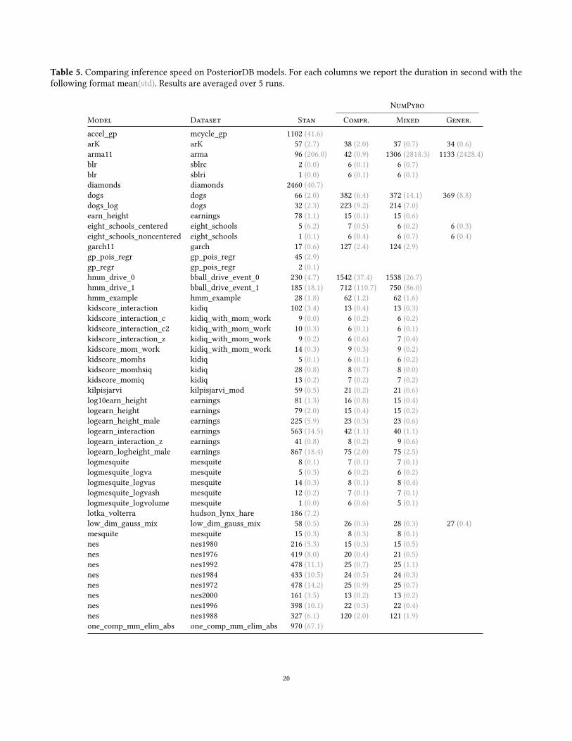
Table 5. Comparing inference speed on PosteriorDB models. For each columns we report the duration in second with the

following format mean(std). Results are averaged over 5 runs.

NumPyro

Model Dataset Stan Compr. Mixed Gener.

accel_gp mcycle_gp 1102 (41.6)

arK arK 57 (2.7) 38 (2.0) 37 (0.7) 34 (0.6)

arma11 arma 96 (206.0) 42 (0.9) 1306 (2818.3) 1133 (2428.4)

blr sblrc 2 (0.0) 6 (0.1) 6 (0.7)

blr sblri 1 (0.0) 6 (0.1) 6 (0.1)

diamonds diamonds 2460 (40.7)

dogs dogs 66 (2.0) 382 (6.4) 372 (14.1) 369 (8.8)

dogs_log dogs 32 (2.3) 223 (9.2) 214 (7.0)

earn_height earnings 78 (1.1) 15 (0.1) 15 (0.6)

eight_schools_centered eight_schools 5 (6.2) 7 (0.5) 6 (0.2) 6 (0.3)

eight_schools_noncentered eight_schools 1 (0.1) 6 (0.4) 6 (0.7) 6 (0.4)

garch11 garch 17 (0.6) 127 (2.4) 124 (2.9)

gp_pois_regr gp_pois_regr 45 (2.9)

gp_regr gp_pois_regr 2 (0.1)

hmm_drive_0 bball_drive_event_0 230 (4.7) 1542 (37.4) 1538 (26.7)

hmm_drive_1 bball_drive_event_1 185 (18.1) 712 (110.7) 750 (86.0)

hmm_example hmm_example 28 (1.8) 62 (1.2) 62 (1.6)

kidscore_interaction kidiq 102 (3.4) 13 (0.4) 13 (0.3)

kidscore_interaction_c kidiq_with_mom_work 9 (0.0) 6 (0.2) 6 (0.2)

kidscore_interaction_c2 kidiq_with_mom_work 10 (0.3) 6 (0.1) 6 (0.1)

kidscore_interaction_z kidiq_with_mom_work 9 (0.2) 6 (0.6) 7 (0.4)

kidscore_mom_work kidiq_with_mom_work 14 (0.3) 9 (0.3) 9 (0.2)

kidscore_momhs kidiq 5 (0.1) 6 (0.1) 6 (0.2)

kidscore_momhsiq kidiq 28 (0.8) 8 (0.7) 8 (0.0)

kidscore_momiq kidiq 13 (0.2) 7 (0.2) 7 (0.2)

kilpisjarvi kilpisjarvi_mod 59 (0.5) 21 (0.2) 21 (0.6)

log10earn_height earnings 81 (1.3) 16 (0.8) 15 (0.4)

logearn_height earnings 79 (2.0) 15 (0.4) 15 (0.2)

logearn_height_male earnings 225 (5.9) 23 (0.3) 23 (0.6)

logearn_interaction earnings 563 (14.5) 42 (1.1) 40 (1.1)

logearn_interaction_z earnings 41 (0.8) 8 (0.2) 9 (0.6)

logearn_logheight_male earnings 867 (18.4) 75 (2.0) 75 (2.5)

logmesquite mesquite 8 (0.1) 7 (0.1) 7 (0.1)

logmesquite_logva mesquite 5 (0.3) 6 (0.2) 6 (0.2)

logmesquite_logvas mesquite 14 (0.3) 8 (0.1) 8 (0.4)

logmesquite_logvash mesquite 12 (0.2) 7 (0.1) 7 (0.1)

logmesquite_logvolume mesquite 1 (0.0) 6 (0.6) 5 (0.1)

lotka_volterra hudson_lynx_hare 186 (7.2)

low_dim_gauss_mix low_dim_gauss_mix 58 (0.5) 26 (0.3) 28 (0.3) 27 (0.4)

mesquite mesquite 15 (0.3) 8 (0.3) 8 (0.1)

nes nes1980 216 (5.3) 15 (0.3) 15 (0.5)

nes nes1976 419 (8.0) 20 (0.4) 21 (0.5)

nes nes1992 478 (11.1) 25 (0.7) 25 (1.1)

nes nes1984 433 (10.5) 24 (0.5) 24 (0.3)

nes nes1972 478 (14.2) 25 (0.9) 25 (0.7)

nes nes2000 161 (3.5) 13 (0.2) 13 (0.2)

nes nes1996 398 (10.1) 22 (0.3) 22 (0.4)

nes nes1988 327 (6.1) 120 (2.0) 121 (1.9)

one_comp_mm_elim_abs one_comp_mm_elim_abs 970 (67.1)

20