Competitive Off-equilibrium: Theory and Experiment * ELENA ASPAROUHOVA, PETER BOSSAERTS, and JOHN LEDYARD ABSTRACT We propose a Marshallian model for price and quantity adjustment in parallel continuous double auctions. Investors submit orders only for small quantities, and at prices that max- imize the local utility improvements. Pareto optimality, on which equilibrium asset pricing theory is built, is eventually reached. Experiments designed with the CAPM in mind show that, consistent with the theory (i) contrary to the standard Walrasian price adjustment model, price changes cross-autocorrelate with excess demands depending on covariances of liquidating dividends; (ii) a risk-weighted endowment portfolio is closer to mean-variance optimality than the market portfolio; (iii) individual portfolios are under-diversified, and more so when dividend covariances are positive. JEL Classification: G11, G12, G14 Keywords: Asset pricing theory, Experimental Finance, Walrasian Equilibrium, Local Marshallian Equilibrium, Price Discovery.

Welcome message from author
This document is posted to help you gain knowledge. Please leave a comment to let me know what you think about it! Share it to your friends and learn new things together.
Transcript

Competitive Off-equilibrium: Theory and Experiment∗
ELENA ASPAROUHOVA, PETER BOSSAERTS,
and JOHN LEDYARD
ABSTRACT
We propose a Marshallian model for price and quantity adjustment in parallel continuous
double auctions. Investors submit orders only for small quantities, and at prices that max-
imize the local utility improvements. Pareto optimality, on which equilibrium asset pricing
theory is built, is eventually reached. Experiments designed with the CAPM in mind show
that, consistent with the theory (i) contrary to the standard Walrasian price adjustment
model, price changes cross-autocorrelate with excess demands depending on covariances of
liquidating dividends; (ii) a risk-weighted endowment portfolio is closer to mean-variance
optimality than the market portfolio; (iii) individual portfolios are under-diversified, and
more so when dividend covariances are positive.
JEL Classification: G11, G12, G14
Keywords: Asset pricing theory, Experimental Finance, Walrasian Equilibrium, Local
Marshallian Equilibrium, Price Discovery.

General equilibrium theory (see, e.g., Campbell (2000)) has become the accepted model for
competitive markets, and thus the lens through which those markets are analyzed. The
economics and the finance branches of the literature appear, however, to have zoomed in
on different properties of the underlying model (see Magill and Quinzii (1996)). The former
is predominantly concerned with the existence of equilibrium and its (Pareto) optimality
properties1, while the latter has focused on the equilibrium pricing relationships.
In relation to its finance application, Cochrane (2001) refers to the general equilibrium
models as the purest example of “the absolute approach to asset pricing,” where “we price
each asset by reference to its exposure to fundamental sources of macroeconomic risk.” And
while the empirical shortcomings of the standard asset pricing models are well recognized,
the tenet of equilibrium has remained intact in the recent theoretical developments aiming
at addressing those shortcomings.2
The classical example of a widely studied class of asset pricing models is the class of
portfolio-based models, where the price of each security is determined relative to some bench-
mark. In the Capital Asset Pricing Model (CAPM), for instance, the prediction is that all
assets are priced such that the market portfolio is mean-variance optimal, i.e., it provides
the maximum expected return for its risk, as measured by the variance of its returns.
A long standing criticism of the equilibrium approach, accompanying it since its incep-
tion (see Walras (1874-77) and Marshall (1890)), is that it is silent about the adjustment
process through which markets arrive at the equilibrium prices and allocations. Without the
understanding of when and how it happens, the properties of the empirical tests would de-
pend on the choice of sampling frequencies for the pricing data. Indeed, unless one assumes
that markets are always in equilibrium, there is little evidence that end-of-period prices and
holdings present anything but arbitrary points in the adjustment process. If that is the case,
it should not come as a surprise that the end-of-month market portfolio is not mean-variance
optimal and that investors are under-diversified, in violation of the CAPM.
1

The extant asset pricing literature has dealt with the negative empirical findings by aug-
menting the model with, among others, more complex individual preferences, less demanding
cognitive processes, and richer stochastic environments. Contributing to this literature and
addressing the criticisms of the equilibrium approach, here we study the possibility for im-
posing reasonable pricing restrictions even off equilibrium. Specifically, this paper proposes a
theory of price discovery in the context of simultaneous multiple markets along with a rigor-
ous experimental test. In the spirit of the CAPM and other factor models, we theoretically
identify and empirically confirm the existence of a portfolio that continuously determines
the prices of all securities even while markets are off equilibrium.
Both in the theory and in the experiment, our aspiration is for markets to achieve Pareto
optimality, a weaker condition than insisting that markets converge to the global equilibrium
of the economy.3 Aside from its desirability from a social welfare point of view, Pareto
optimality is a necessary condition for a sensible off-equilibrium asset pricing model. With it,
we can establish a clear parallel between the proposed theory and the standard representative
agent equilibrium model.4
The proposed theory employs local competitive equilibrium concepts that require that
only small orders be submitted. The market organization we focus on is the continuous dou-
ble auction (CDA). Controlled experiments have long demonstrated that the CDA facilitates
convergence to Pareto efficient allocations.5 Within this market institution trade happens
at prices that have not yet equilibrated. At the same time, final allocations are shown to be
optimal–not only in simple one-market settings as in Smith (1962) but also in much more
complex, multi-market environments, as in Plott (2001).
We focus on the CDA and ask: what is the mechanism that drives the changes in prices
and allocations? Thus, the goal in this paper is to model and explain how rational agents
behave in examples of the CDA and not necessarily how those agents should behave.
The leading assumption of the model, on which we elaborate later, is that trade intensity
is the highest for those agents who are willing to pay the most or accept the least for the
2
traded goods/assets. Specifically, investors submit bids that monotonically relate to their
initial marginal valuations of the assets. All transactions occur at a local equilibrium price,
equal to the average of all bids. As imposed by the above assumption, those with more
to gain (i.e., those with the largest difference between their bid and the average bid) trade
faster. Then the process repeats but with now changed (due to the executed trades) marginal
valuations for the traded assets. Agents at all times make offers that, if executed, would
secure maximal local growth in their utilities. We call this a “local Marshallian equilibrium”
theory as it is in the spirit of Marshall (1890).
Guided by an important interplay between theory and experimental evidence, we study
two versions of this theory. The first one we call “the original Marshallian adjustment,”
where prices and quantities adjust concurrently. In the second, that we call the “lagged
theory,” prices move faster than agents are able to adjust their offer quantities. We derive
implications for price and allocation dynamics in the two settings and study the validity
of these implications in a controlled experiment that is known to generate the CAPM (see
Asparouhova, Bossaerts and Plott (2003)). While the paper presents the theory in its most
general form, the main theoretical and empirical findings are best illustrated in the simple
setup of this experimental economy.
In our experiments, participants start with a portfolio of two risky assets, called A and B,
a risk free asset, called N (notes), and some cash. During a short period of time (15 minutes
or less), they can trade in a anonymous, computerized, continuous open-book system. The
goal is to trade to an optimal portfolio of assets and cash. This optimum depends on the
participants’ objective function that is assigned by us, the experimenters. Participants only
know their own incentives and that everyone else has equal access to the computerized
markets. After markets close, participants are paid real money depending on how close their
final allocations are to their optimum.
In the theory we show that individual allocations converge towards a Pareto optimal
point. On the path towards Pareto optimality, the portfolio with the highest Sharpe ratio
3
is easily identifiable. This portfolio converges to the market portfolio of stocks A and B
only at the end. On the convergence path, the weight on each stock is proportional to the
average holding of that stock across investors. With this weighting scheme, higher weights
are attributed to those investors who are more risk averse. We call the portfolio “the risk-
aversion-weighted endowment” (RAWE) portfolio. As the adjustment process approaches
Pareto optimality, the RAWE portfolio converges to the market portfolio of Stocks A and
B.
Asset pricing is consistent with the Marshallian model if the RAWE portfolio has the
highest Sharpe ratio. Conversely, assuming that the economy is in a local Marshallian
equilibrium, one can use the RAWE portfolio to price the traded assets.
In the lagged theory an important regularity emerges along the equilibration path. Price
changes in one asset correlate positively with excess demand in the other asset when asset
payoffs (liquidating dividends) are positively correlated. Price changes anti-correlate with
excess demand when the asset payoffs are negatively correlated. This relationship induces
cross-autocorrelations in price changes. Lo and MacKinlay (1990) show that such cross-
autocorrelations might be behind momentum in returns. Empirically, Lewellen (2002) shows
that indeed those cross-correlations play an important role.
Turning to the empirical tests, we first document to what extent trading through the
continuous open-book system improves the collective welfare. In our setting, there is a
unique allocation that provides maximum total gains. Hence, we compare payoffs at initial
endowments with payoffs at final holdings, after markets close. We also compare the final
payoffs against the hypothetical maximal possible total payoffs. While significants gains
from trade are realized, we find that the final allocations fall short of fully achieving Pareto
optimality.
We test the original vs. the lagged adjustment theories and find that price changes are
better explained by the lagged theory of adjustment. To enable such tests, we have two
market conditions. One is where stock A and B’s payoffs are positively correlated, and the
4

other is where they are negatively correlated. Our results provide overwhelming support for
the prediction that prices and excess demands for securities cross-correlate according to the
sign of the payoff correlation. Price dynamics of Stock A and B change significantly and
according to the sign of the payoff correlations. This evidence is consistent with the lagged
theory but not with the original adjustment theory.
The optimality of the RAWE weighted portfolio, predicted by the lagged theory, is also
upheld in our experiments, though the evidence is less clear when the payoff correlation
between stocks A and B is positive. As we pointed out above, one can turn around these
findings, and use at any time the RAWE-weighted portfolio in order to predict prices–the
price configuration should be such that the RAWE weight portfolio is optimal.
Since participants fail to fully exploit potential gains, the market adjustment process is
incomplete. Consequently, final holdings provide a snapshot of the adjustment process before
full Pareto optimality is reached. If our theoretical predictions are true, then final holdings
across the two treatments (positive and negative payoff correlations between stocks A and B)
should be significantly different. Specifically, we expect individual portfolios of Stocks A and
B to be closer to the market portfolio when correlations are negative. This is exactly what
we find, and it is in line with the behavioral finance finding of investor under-diversification.
Our findings have implications for the organization of centralized markets. Specifically,
frequent (in our case continuous) clearing is important, and markets need to be competitive
for small quantities. This way, markets manage to exploit the local optimization that partic-
ipants resort to, and push trades in the direction of maximum utility improvements. Many
electronic stock markets in the world (like Euronext and NYSE) are organized as continuous
double auctions. In a call market like the London Gold Market, however, participants can-
not make gradual adjustments in the direction of maximal gains; instead, all exchanges have
to take place at once, at prices that are determined by a lengthy Walrasian tatonnement
process (meaning that prices are adjusted in the direction of excess demand). As such, “free
markets” per se would not guarantee optimal allocations, instead, the rules of engagement in
5

the exchange process are what is crucial for Pareto optimality to emerge. This is related to a
robust finding from experimental economics (see Smith (1989)), that only specific exchange
mechanisms generate the competitive equilibrium.
Our findings also imply that the widely held belief that market prices adjust in the direc-
tion of excess demand (prices increase when there is excess demand; decrease when there is
excess supply) does not necessarily apply, at least as far as the continuous double auction is
concerned. Cross-correlation between price changes and excess demand in other assets con-
found this relationship. At times, the confounding effect can be sufficiently severe for there
to be no (simple) correlation between price changes and excess demand (see Asparouhova,
Bossaerts and Plott (2003) and Asparouhova and Bossaerts (2009)).
I. Background
Theoretically, out-of-equilibrium market behavior has been described by two alternative
dynamic models, the Walrasian and the Marshallian. The predominant one has by and large
been the Walrasian model, described with the aid of the fictitious aucitoneer and the corre-
sponding tatonnement process. In this process, upon announcement of a price, all traders
submit their desired orders which are awarded execution if there is no excess demand, or else
the price is adjusted in the direction of the excess demand. No exchange takes place before
prices reach equilibrium. The Marshallian adjustment process is described by Leijonhufvud
(2006) as “what we today label agent-based economics. Recall that Marshall worked with
individual demand-price and supply price schedules. [And] the demand-price and supply
price schedules give rise to simple decision-rules that I like to refer to as “Marshall’s Laws
of Motion.” For consumers: if demand-price exceeds market price, increase consumption; in
the opposite case, cut back.”6
A lot of the theoretical effort has been expended in finding constraints on preferences
that would ensure that the adjustment processes converge to the Walrasian equilibrium. A
6

rather small fraction of the equilibration literature, but most relevant to our study, is the
one that has studied the possibility of out-of-equilibrium trading and the conditions that
must be imposed on the trading rules to guarantee that the economy arrives at a Pareto
optimal allocation (e.g., Negishi (1962), Hahn and Negishi (1962), Uzawa (1962), Hurwicz,
Radner, and Reiter (1975), Friedman (1979), and Fisher (1983)). A formal overview of
General Equilibrium, Walrasian and Marshallian dynamics is provided in Section A of the
Appendix.
The market organization we focus on is the continuous double auction (CDA). Controlled
experiments have long demonstrated that the CDA facilitates emergence of Pareto efficiency,
see Smith (1962) and Plott (2001). What makes Pareto efficiency extremely demanding
from a central planner’s point of view, is that beneficial re-allocations require full knowledge
of every individual’s preferences. At the same time the institution of continuous double
auction is known to generate Pareto optimality without anyone having knowledge of others’
preferences. To accomplish this, markets effectively need to solve a set of, often highly
nonlinear, equations the parameters of which no individual participant knows. In this paper
we aspire to provide a model that explains the above equilibration dynamics in a CDA as
the aggregation of locally optimal choices of individuals.
In the continuous double auction, individuals (agents; participants) can submit bids (to
buy) or asks (to sell) at any price, and whenever the highest bid is at a price above the lowest
ask, a trade takes place immediately. In modern instances of the double auction, called the
open-book system, bids and asks that are surpassed by more competitive orders (bids at a
higher price or asks at a lower price) remain available for later, unless they are canceled.
The open book system is the preferred exchange mechanism of financial markets around the
world, and in particular, stock exchanges (NYSE, Euronext, LSE, NASDAQ, etc.).
7

II. Some Sylized Facts From Experiments
Before proceeding with the proposed theory, we present some experimental evidence as
it relates to the adjustment models.
A. The Structure of Market Experiments
For those unfamiliar with markets experiments, a brief introduction follows. Participants
are solicited, usually via email invitations, to come and participate in an experimental session
at a given location (or, in some instances, access the experiment online) and at a given time.
Each experimental session starts with an instructional period, where the rules of engagement
are explained, participants are given the opportunity to ask questions, and some practice
takes place. An experiment proceeds in a series of replications, called periods. At the
beginning of a period each participant i is given an initial endowment of commodities (or
financial assets), wi. Markets open and participants are free to trade subject to the usual
budget constraints. Trading occurs via a market institution of the experimenter’s choice.
At the end of a period, participant i will have traded di and will have final holdings of
xi = wi + di. Participants receive payments according to a payoff function ui(xi), specified
by the experimenter and presented to the participants during the instructional period. In
some experiments all periods are payoff-relevant. In others, participants go over several
periods and only some are chosen at random to be payoff-relevant.
Two standard trading institutions used in experiments are the Continuous Double Auc-
tion (CDA) and the Call Market (CM). The CDA is a trading process in which participants
post buy and sell offers by specifying quantity and price. In most cases the offers are dis-
played in an open book, i.e, they are visible to all participants. (In dark pools, not discussed
in this paper, only some, if any, of the offers are publicly displayed.) Those offers can be ac-
cepted by others. When accepted an offer becomes part of a transaction and it is withdrawn
8

from the order book. The CDA can be thought as an example of a system that facilitates
non-tatonnement dynamics.
In a call market, participants also post buy and sell offers by specifying quantity and
price but, contrary to the CDA, no transaction occurs or is accepted until the market is
“called.” If the book is closed (i,e, subjects cannot see each others’ bids), this is just a sealed
bid auction. If the book is open (i.e., participants can see each others’ bids) and subjects
can withdraw their bids and submit new ones, then this system facilitates the tatonnement
dynamics.
B. Findings from Market Experiments
Easley and Ledyard (1992) examines data from single-commodity CDA markets (pre-
sented in a partial equilibrium setting to the participants but equivalent to an environment
with two commodities and quasi-linear preferences). These markets involve a series of peri-
ods with period-invariant payoff functions. The authors study the upper and lower bounds
on prices for each period. They find that bounds respond from period to period as pre-
dicted by the Walrasian model–that is, after a period with excess demand at the upper
bound, the upper bound at the following period would be higher. They also find that prices
within a period respond to the participants’ marginal willingness to pay (accept), as in the
“Marshallian” dynamic system. Finally, they find that initial trades respond stronger to
excess demands at the previous period’s price bounds while later trades respond more to
local information such as the gradients of the utility/payoff functions. Thus, initial trades
within a period seem to be guided by Walrasian dynamics, while later trades are guided by
Marshallian dynamics.
Anderson, e.a. (2004) examines the dynamic behavior of prices in the context of environ-
ments closely related to those in Scarf (1960). These are particularly interesting environments
in that the Walrasian dynamic does not always lead prices to converge to the unique market
9

equilibrium. The experiments also involves a series of periods. A quick summary, that does
not do justice to the paper, is that across-period price dynamics are consistent with the
Walrasian tatonnement and within-period price dynamics are not. More precisely, average
prices move from period to period in a manner predicted by the tatonnement model, even
though the CDA is not a tatonnement system. On the other hand, Anderson, e.a. (2004)
uncover no such relationship for within-period trades and prices. The data from the reported
experiments does not conform to either the standard Walrasian or Marshallian models (both
of which are presented in section A.3 in the Appendix).
Biais, Bisiere, and Pouget (2013) study the effect of preopening mechanisms in experi-
mental markets. They find that when call auctions are preceded by a binding preopening
period, subsequent gains from trade are maximized. Pouget (2007) studies experimentally
the institutions of call market and the Walrasian tatonnement and finds that the latter is
more conducive to learning of the equilibrium strategies.
A detailed overview of experimental findings on market equilibration dynamics is provided
in Crockett (2013).
At this point our main question remains open: what is the mechanism by which prices
and quantities are driven in a CDA?
III. An Informal Version of Our Theory
We posit that individuals follows a simple rule that is well adapted to the continuous
double auction as long as it is “competitive in the smalls.” It means that, as long as everyone
submits orders for small quantities, individuals cannot influence where the market is going–
i.e., they take the aggregate order arrivals and order prices as given. This simplifies market
interactions: individuals cannot manipulate the market and thus they do not need to think
strategically. The assumption of small orders is reasonable when markets are comprised
10

of many traders each with a small endowment in comparison to the aggregate endowment,
and each lacking the structural knowledge (other traders’ positions, preferences, strategic
sophistication, etc.) needed to successfully manipulate the market by submitting a large
order. Empirically, competition with small orders is documented in institutional trading, see
Rostek and Weretka (2015).7
We propose a theory of Marshallian adjustments where individuals express willingness
to trade in the direction that provides the biggest local improvement to their portfolio, at
prices that reveal their true valuation for the proposed trades. We assume that agents with
higher willingness to pay or lower readiness to receive trade more intensely. Similar in spirit
to this trading intensity assumption, the model of Rostek and Weretka (2015) delivers an
equilibrium prediction that agents (who are firms in the model) submit demands in small
orders, and those facing the highest gains from trade transact more quickly. This procedure
necessarily achieves Pareto optimality in its asymptotic resting point.
The Marshallian Local Theory raises a practical issue. Price adjustment in CDAs often
occurs at a speed far beyond the speed of adjustment of individual orders. By the time an
agent has canceled old orders and submitted new orders, prices may have changed a number
of times. So, we investigate what happens if offers move with a lag compared to prices.
While more practically appealing, this model sacrifices a Pareto optimal destination in the
most general case. There is, nevertheless, a case of interest in which convergence to Pareto-
optimal allocations can be proven. This is the case of quasi-linear preferences that are the
preferences employed for the CAPM model of finance.
IV. A Formal Local General Equilibrium Theory
In this paper, we advance an equilibration theory for markets where price-taking only
applies to small orders. At its core is the assumption that, to avoid adverse price movements,
11
agents only submit small orders that are optimal locally. Therefore, we shall call it local
general equilibrium theory.
Before presenting the local theory, we present the standard global General Equilibrium
Theory for exchange economies.
A. Global Exchange Environments
There are I consumers, indexed by i = 1, . . . , I, and K = 1 +R commodities, where the
last R commodities are indexed by k = 1, . . . , R. We reserve the first commodity as a special
one, and will designate it as the numeraire commodity when needed.
Each i owns initial endowments ωi = (ωi1, . . . , ωiK) such that ωik > 0 for all i and k.
Let xi = (si, ri1 . . . , riR) be the consumption of i and let X i = xi ∈ <K | xi ≥ 0 be the
admissible consumption set for i. Let di ∈ <K be a vector of net trades. i’s consumption
equals her initial endowments plus net trades, xi = ωi + di. Finally, each i has a quasi-
concave utility function, ui(xi). We will assume that ui ∈ C2 (that is, it has continuous
second derivatives) although many of our results would hold under weaker conditions. We
also assume that xi|ui(xi) ≥ ui(wi) ⊂ Interior(X i).
A.1. Global General Equilibrium
Let p be the vector of prices, p = (p1, ..., pK) for the K assets. The excess demand of i is
ei(p, ωi) = arg maxdi ui(ωi + di) subject to p · di = 0 and wi + di ∈ X i. The aggregate excess
demand, of the economy, is e(p, ω) =∑ei(p, ωi).
12

Competitive market equilibrium in an exchange economy is straight-forward to describe.
A price, p∗, and a vector of trades, d∗ = (d∗1, ..., d∗I) is a market equilibrium if and only if
(1) given prices p∗ trades d∗i are optimal for all i = 1, ..., I and (2) markets clear, i.e.,
d∗i = ei(p∗, ωi),∀i = 1, ..., I.
and
e(p∗, ω) = 0.
B. Local Exchange Environments
A local exchange economy at time t is described by the local allocation, xi(t) = wi +
di(t), a set of feasible local trades, F i(xi(t)) = ηi ⊂ <K , and the local utility function,
∇ui(xi(t)) ·ηi. Feasibility requires that∑
i ηi = 0. In this local economy there is a temporary
local equilibrium.
The dynamics are described by the movement through time from one local equilibrium to
the next. We discuss a Marshallian theory below. A Walrasian theory along with an equiv-
alence result between the two theories (under certain conditions) are presented in Sections
B.1 and B.2 respectively of the Appendix.
B.1. A Local Marshallian Theory
Samuelson (1947) (p. 264) describes a Marshallian dynamic of quantity adjustment, as
opposed to the Walrasian price adjustment, as follows. “If ‘demand price’ exceeds ‘supply
price,’ the quantity supplied will increase.”8
In this section, we propose a dynamic process that relies on the Marshallian intuition.
Early versions of allocation mechanisms based on this intuition can be found in Ledyard
(1971) and Ledyard (1974).
13
It is easiest to incorporate a Marshallian approach into a general equilibrium model if
we adopt the concept of “numeraire.” Such an approach will later render the finance model
a straight-forward special case. For the rest of this paper, we assume that commodity 1 is
the numeraire, and ui1(xi) > 0,∀xi. Let p = (1, q) and xi = (si, ri) ∈ < × <R+. Here si is i’s
quantity of the numeraire commodity.
We will let ρik,t denote the marginal rate of substitution between commodities 1 and k at
time t, k = 1, ..., R (i.e, ρik,t =∂ui(xit)/∂x
ik
∂ui(xit)/∂xi1), representing i’s marginal willingness to pay for rk
in units of commodity 1. Let ρit = (ρi1,t, ..., ρiR,t).
Let bik,t be the amount that i expresses to the market about their willingness to pay or
accept.9 Also, let bit = (bi1,t, ..., biR,t).
Marshallian assumption. Quantities move towards those who are prepared to offer
the higher surplus, relative to the market. Formally, over a time period τ , i’s trades will be
∆rit = rit − rit−τ = α(bit − qt), where α is the rate at which surplus is translated into trade.
Local budgets balance. Locally, each individual has to balance their budget, which
implies pt ·∆xit = 0, or qt ·∆rit + 1 ·∆sit = 0, or ∆sit = −qt ·∆rit.
Local approximation. Since, locally ∆uit ≈ ∇uit∆xit, using ∆sit = −qt · ∆rit, the
Marshallian assumption, and uik,t = ρk,tui1,t we derive ∆uit ≈ ui1,t(ρ
it − qt)∆r
it = ui1,t(ρ
it −
qt)α(bit − qt).
Competitive (no speculation) assumption. Since this is a model of competitive
behavior, we maintain the basic assumption that individuals take the price qt, as well as
the Marshallian assumption, as given. Faced with this prospect, how should an individual
choose their bid, bit? Individual i wants to make ∆uit = uit−uit−τ > 0 large, if at all possible.
Therefore i wants to choose bit so that bit − qt = ciτ(ρit − qt) where ciτ is chosen to control
the rate at which i will trade. Since this is a linear approximation of the individual’s utility
increase, she will not want ciτ to be too large.10
14

With these bids and this trading dynamic, trading is feasible if and only if∑
i ∆rit = 0.
This is true if and only if qt =∑
i ciρit∑
i ci = ρt. We can think of qt as the local Marshallian
“equilibrium price.” It is the only price at which individuals will not want to change their
bids, given the Marshallian trade dynamic.
To summarize, we have
∆ri = α(bi − q) (1)
bi = q + ciτ(ρi − q) (2)
∆si = −q∆ri (3)
qk =
∑i ciρik∑i ci
(4)
.
Substitute (2) into (1) and let τ → 0. This leads to a continuous-time local Marshallian
equilibrium theory:
drik(t)
dt= αci(ρik − qk) (5)
dsi(t)
dt= −qdr
i(t)
dt(6)
qk =
∑i ciρik∑i ci
(7)
Remark 1: The above is a “reduced form” competitive theory. It assumes that traders are
taking two things as given: (i) prices q and (ii) the trading rule ∆ri = rit−rit−τ = α(bi−q). If i
behaves competitively, then i takes q as given and chooses bi = q+ciτ(ρi−q). Summing across
i on both sides of this response equation and dividing by I yields b = q + (τ/I)∑ci(ρi − q).
Therefore, in equilibrium, q = b = ρ.
15

In a CDA system, transactions take place when someone’s bid/ask is accepted. So on
average the transaction price will be b. Also, traders with the most to gain, those with the
largest difference in bi− b, will trade faster than others. Thus trade should occur, on average,
according to the process we described above. That is, (5)-(7) can be loosely thought of as the
expected value of a stochastic process whose absorbing states are the rest points of (5)-(7).11
Theorem 1: (Convergence to Pareto Optimality)
Let x(t) = [r(t), s(t)]. For the dynamics in (5)-(7), [x(t), p(t)] → (x∗, p∗) where x∗ is
Pareto-optimal and e(p∗, x∗) = 0.
The proof of the theorem is relegated to Section C of the Appendix.
C. Introducing a Lag
The Marshallian Local Theory of the previous section raises a practical issue. Price
adjustment in CDAs often occurs at a speed far beyond adjustment of individual orders.
By the time an agent has canceled old orders and submitted new orders, prices may have
changed a number of times. So, let us investigate what happens if bidders submit orders in
reference to lagged and not to current prices.
C.1. The Model
We maintain all assumptions of Section IV.B.1, except for allowing for slow bid adjust-
ment, i.e,
bit = qt−τ + τci(ρit − qt−τ ).
Thus, while agents take into account their marginal valuations at current holdings, they
respond optimally to lagged prices, and not to the current prices. As before, ∆rit = rit−rit−τ =
α(bit − qt), and as a result qt = (1/I)∑bit will clear the markets.
16

This implies,
qt = qt−τ + τ
∑i ci
I(ρt − qt−τ ) (8)
rit = rit−τ + ατ [ci(ρit − qt−τ )−∑
j cj
I(ρjt − qt−τ )]. (9)
Letting τ → 0,
dri(t)
dt= α[ci(ρit − qt)− c(ρt − qt)] (10)
dq(t)
dt= −c(qt − ρt) (11)
Compare this to (5)-(7). First, in (7) prices q adjust instantaneously to the weighted average
willingness to pay ρ, while in (11) prices q converge exponentially to ρ. Second, in (5)
allocations adjust, according to the Marshallian intuition, proportionally to the individual
difference in the willingness to pay and the market price. In (10), the Marshallian adjustment
is modulated by the difference between the average willingness to pay and the market price.
If prices adjusted immediately this last term would vanish and we would have exactly (5).12
C.2. Asymptotics
If we try to proceed as in Theorem 1, we immediately run into a problem. With lags,
dui(t)/dt = ui1(ρi − q)(dri
dt) = ui1(ρ
i − q)α[ci(ρi − q) − c(ρ − q)] = ui1[(ρi − q)αci(ρi − q)] −
ui1[(ρi − q)αc(ρ − q)]. While the first term is positive as long as ρi 6= q), the second term
is not necessarily so. Thus, it is possible that along the dynamic path some individual
utilities might decline because of the lag in the response to prices. Thus, we cannot expect
convergence to occur in as orderly a manner as occurred in Theorem 1.
There is, nevertheless, a case of interest in which convergence to Pareto-optimal alloca-
tions can be proven. This is the case of quasi-linear preferences where ui1 = 1 for all i. This
17

is true, for example, for the CAPM model of finance. There are also a lot of (experimental)
data for this case.
Theorem 2: (Convergence to Pareto Optimality)
Let x(t) = [r(t), s(t)]. If (i) there are no income effects, i.e., ui1(xi) = 1 for all i and all
xi ∈ X, and (ii) xi(t) > 0 for all t, then for the dynamics in (10) and (11), [x(t), p(t)] →
(x∗, p∗) where x∗ is Pareto-optimal and e(p∗, x∗) = 0.
The proof of this theorem is relegated to Section C of the Appendix.13
C.3. Cross-autocorrelations
In our model, prices change in reaction to the average willingness to pay or receive
(see (11)). Respectively, each trader’s willingness changes with how his/her holdings evolve
as a result of the trade opportunities (see (10)). With the system (10)-(11) guiding the
market motion, a rich pattern of price dynamics is possible. In particular, it generates
interesting cross-autocorrelations that, like the cross-security effects of excess demands on
price changes, depend on payoff covariances. Cross-autocorrelation intensities also depend
crucially on adjustment parameters, such as α, τ and cis.
Cross-autocorrelations have been recorded in historical field data and are thought to
be the key factor behind the momentum effect, i.e., the finding that prior-year winners
outperform prior-year losers, even after adjusting for standard risk premia (see Lewellen
(2002)). In our equilibration model, cross-autocorrelations emerge because of the complex
local adjustment dynamics: prices of some securities may adjust faster than others, because
trade in them leads to higher utility increases. The problem is, however, that few general
principles govern the price-allocation evolution embodied in the differential equations in
(10)-(11). In particular, cross-autocorrelation properties depend crucially on adjustment
parameters such as ci. Conversely, cross-autocorrelation properties could be used to identify
those parameters in ways that evolution of individual prices could not.
18

The presence of cross-autocorrelations raises an intriguing question: since such cross-
autocorrelations imply opportunities to profit from, e.g., pairs trading as in Gatev, Goetz-
mann, and Rouwenhorst (2006), why would they not disappear? If exactly the same situation
is replicated period after period, we expect prices to gradually start out closer to equilib-
rium, and hence, cross-autocorrelations to be reduced. However, if every period parameters
(endowments, risk penalties, payoff patterns) change in unknown ways, there is insufficient
time for market participants to fully learn the cross-autocorrelations; by the time these auto-
correlations are estimated with sufficient precision, they will have moved away. As a result,
hindsight will reveal significant cross-autocorrelations, but they cannot be exploited out-of-
sample. Bossaerts and Hillion (1999) indeed show robust evidence of in-sample predictability
in historical return data that cannot be exploited out-of-sample. In appears that the only
way to robustly capture cross-autocorrelations is through momentum portfolios. However,
the presence of cross-autocorrelations is not a foregone conclusion, and hence, momentum
effects may come and go. We leave it to future analysis to determine more precisely the
relationship between models of price discovery and momentum.
V. Experimental Evidence
Here, we return to experiments. The payoff to participants in those experiments is
according to quasi-linear, quadratic functions, like those underlying the Capital Asset Pricing
Model (CAPM) in finance.
A. Experimental Setup
Each experiment consists of a number of independent replications of the same situation,
referred to as periods. At the start of a period, participants are given an initial position in
three securities, referred to as A, B and Notes, and some cash. The markets for the three
19

securities are simultaneously open for a pre-set amount of time. The trading interface is a
fully electronic web-based version of a CDA, whereby non-marketable orders remain in the
open book of the market. After markets close, at the end of a period, participants receive
payoffs according to the given payoff function, minus a fixed, pre-determined loan payment.
After their liquidating payoff all three securities expire worthless. The total payoff from an
experimental session equals the sum of the payoffs across the periods.
Participants did not have to be present in a centralized laboratory equipped with com-
puter terminals, but could instead access the trading platform over the internet. Communi-
cation in experiments like these takes place by email, phone and through the announcement
and news page online. Each session had between 30 and 42 participants. We should note
that those numbers are 30-50% larger than a typical market experiment. The scale is chosen
to ensure a trading environment that best approximates the conditions of the theory: large
enough markets so that there is only a small bid-ask spreads but still, small enough markets
so that the best ask and best bid be valid only for small quantities.
End-of-period payoff functions are as follows. Participant i, when holding hi units of the
Notes, Ci of cash and the vector ri of securities A and B receives a payoff
Pay(i) = [ri · µ]− ai
2[ri · Ωri] + Ci + 100hi − Li, (12)
where Li denotes the loan payment.
In the experiments,
µ =
230
200
,and
Ω =
10000 (+/−)3000
(+/−)3000 1400
.
20
The off-diagonal elements of Ω are negative in periods 1 through 4 in the first experiment
(28 Nov 01) and positive in periods 5 through 8. The design is reversed in the other (three)
experiments: the off-diagonal elements are positive in periods 1 through 4 and negative in
periods 5 through 8.
When interpreting µ as a vector of expected payoffs on securities A and B, and Ω as the
(positive definite, symmetric) matrix of payoff covariances, we effectively induce the mean-
variance preferences at the core of the CAPM in finance. ai (> 0) measures the risk penalty.
The change in off-diagonal elements of Ω corresponds to a change in the covariance of the
(random) payoffs on A and B.
Participants in each experimental session are grouped into three types. Each type is
assigned one of three values for the parameter ai, chosen in such a way as to generate similar
pricing as in the earlier CAPM experiments reported in Asparouhova, Bossaerts and Plott
(2003) that use “native” risk aversion. See Table I for details.
Each type also receives a different initial allocation of A and B. Notes are in zero net
supply but short sales are allowed. Participants are not informed of each others’ payment
schedules or initial holdings.14
All accounting is done in an experimental currency called “francs,” converted to dollars
at the end of a session at a pre-announced exchange rate. Each experimental session lasted
approximately three hours and the average payoff was $45 (with range between $0 and $150).
B. The CAPM Equilibrium
Let xi = (si, ri), where ri = (ri1, ri2) are the quantities of A and B that agent i chooses,
and si is quantity of the numeraire good (cash plus payoffs on positions in Notes, minus the
Loan payment). Then:
u(xi, ai) = si + µ · ri − (ai/2)(ri)′Ωri.
21

With the above preferences, it is straight-forward to derive the expressions:
ρi =µ− aiΩri, (13)
ei(q, wi) =(1/ai)Ω−1(µ− q)− wi, (14)
where the excess demand vector ei now includes only the risky securities (not the numeraire
asset).
The global Walrasian equilibrium price and allocations are
q =µ− bΩw (15)
ri =(1/ai)bw (16)
where b = [∑
(1/ai)]−1, and w denotes the per-capita average endowment, w = (1/I)∑wi.
Note that because of the quasi-linearity, the equilibrium holdings r are independent of indi-
vidual endowments wi.
In the CAPM interpretation of this economy, w is referred to as the market portfolio (of
risky securities). The pricing equation (15) captures the essence of the CAPM: it reveals
that the market portfolio will be mean-variance optimal. Indeed, Roll (1977) showed that a
portfolio z satisfies the following relationship for some (positive) scalar β:
q = µ− βΩz, (17)
if and only if z is mean-variance optimal. Notice that this is exactly the form of the equi-
librium pricing formula in (15), so w is mean-variance optimal. On the other hand, the
choice equation (16) exhibits portfolio separation: individual allocations are proportional to
a common portfolio, namely, the market portfolio w.
22
C. Equilibration Predictions
Applying the version of the Marshallian Local Theory where bid adjustment is as fast
as the price adjustment (Section IV.B.1) to the CAPM economy, we get (relegating the
derivation to the Appendix):
dq(t)
dt= (
α∑ci
)∑
(ciai)2Ω2ei[qt, rit]. (18)
That is, price changes are related to weighted average Walrasian excess demands through
the square of the matrix Ω. As such, we expect price changes in one security to be related
not only to the security’s own excess demands, but also to the excess demands of other
securities. The relationship is determined, among others, by the elements of Ω2.
Using (5) and, from (13), ρi − q = µ− q − aiΩri, we get that local allocations follow
dri(t)
dt= αci[µ− qt − aiΩrit]. (19)
Again, adjustment is driven by the matrix Ω.
When bid adjustment is slower than price adjustment (Section IV.C), Equations (10)
and (11) take particularly interesting forms. Price changes are related to (weighted) average
Walrasian excess demands through the matrix Ω (rather than the square):
dq(t)
dt= Ω
∑(ciai)ei(qt, r
it). (20)
Allocation dynamics take the following form:
dri(t)
dt= −αΩ[ciairit −
1
I
∑cjajrjt ] + α(ci − c)(µ− qt). (21)
23

If ci = c, ∀i, that is all i trade with the same aggressiveness, the second term drops out:
dri(t)
dt= −αcΩ[airit −
1
I
∑ajrjt ] = −αc
(ai − 1
I
∑aj)
Ωw. (22)
That is, changes in holdings are a linear transformation of the market portfolio (per-capita
endowment). Except in the unlikely event that the per capita allocation is an eigenvector of
Ω, agents must trade.
In the CAPM setting, where Ω is the matrix of payoff covariances, imagine that Ω is
diagonal. The diagonal elements of Ω are the payoff variances. In that case, volume (the
sum of the absolute value of the elements in dri(t)dt
) will be the highest for the high-variance
securities. That is, most adjustments take place in the high-variance securities. The sign
of the changes in an agent’s holdings of securities depends on value of the parameter ai
relative to the average (1/I)∑aj. Since these coefficients measure risk aversion in a CAPM
setting, this means that the more risk averse agents sell risky securities (the entries of dri(t)dt
are negative); less risk averse agents buy. Effectively, the more risk averse agents unload
risky securities, paying more attention to the most risky securities, because that way their
local gain in utility is maximized. Likewise, less risk averse agents do what is locally optimal:
increase risk exposure by buying the most risky securities first.
When Ω is non-diagonal, the off-diagonal elements equal the payoff covariances, and
the sign of those covariances interferes with the above dynamics. Intuitively, when the off-
diagonal elements are negative, i.e., when the securities’ liquidating payoff covariances are
negative, securities are natural hedges for one another, and the market portfolio provides
diversification. Increasing one’s risk exposure by buying risky securities (or decreasing one’s
risk exposure by selling risky securities) leads to a less diversified portfolio, i.e., to utility
losses. Maximum local gains in utility are obtained by trading combinations of securities that
are closer to the per-capita average endowment, i.e., the market portfolio. As a consequence,
24

agents’ portfolios of risky securities remains closer to the market portfolio than in the scenario
when payoff covariances are zero or positive.
In an experimental setting (unlike in the theory), the equilibration process may not go
all the way to its end.. This may happen when agents do not perceive enough gains to cover
the effort of trading. If this happens, agents will not have traded back to holdings that are
proportional to the per-capita average endowment. In CAPM terms, portfolio separation
would fail (and CAPM equilibrium pricing would not hold).
The role of Ω in this adjustment process is crucial. If the off-diagonal elements of Ω
are positive (payoff covariances are positive), and the equilibration process halts before fully
reaching equilibrium, then violations of portfolio separation can be expected to be larger
than if these off-diagonal elements are negative (payoff covariances are negative).
Remark 2: Were it not for the last term in (21), ci and ai would not be separately identified.
So, identification requires heterogeneous aggressiveness across agents.
D. Experimental Findings
Transaction Prices
Figure 1 displays the evolution of prices of securities A (dashed line) and B (dash-dotted
line).15 Each observation corresponds to a trade in one of the three securities. The prices of
the non-trading securities is set equal to their previous transaction prices. Time (in seconds)
is on the horizontal axis; Price (in francs) is on the vertical axis. Vertical lines separate
periods. Horizontal lines indicate equilibrium prices of A (solid line) and B (dotted line).
Note that their levels change after 4 periods, reflecting the change in the off-diagonal element
of Ω.
25
It is evident from Figure 1 that transaction prices are almost invariably below equilibrium
prices. Also, relative to equilibrium levels, prices generally start out lower in periods when
the off-diagonal terms of Ω are positive.
Price Dynamics
Table II displays the results from projections of within-period changes in transaction prices
of A and B onto the weighted sum of individual Walrasian excess demands. Weights are
given by individuals’ ais.16 The time series data for each experiment is split into two parts,
where one sub-sample covers the periods with positive off-diagonal elements for Ω, and the
other covers the periods with negative off-diagonal elements. All tests are one-sided17 and
the estimates of the slope coefficients of aggregate excess demands are bold-faced whenever
they are significant at the 1% level.
The regression’s R2s are small, but the F -tests reveal that significance is high. The first-
order autocorrelation coefficients of the error term suggests little mis-specification (some are
significantly negative, but one would expect the data to generate a number of significant
autocorrelations even if the true autocorrelation is zero).
We document the following. First, each security’s price changes significantly and posi-
tively correlate with its weighted aggregate excess demand. Second, the signs of the cross-
effects (partial correlation between a security’s price change and the weighted aggregate
excess demand in the other security) are almost always the same as that of the off-diagonal
elements in Ω (if they are not, the projection coefficient is insignificant). The estimation
results are highly significant.18
26

Table II thus suggests that the matrix of coefficients in projections of transaction price
changes onto aggregate (Walrasian) excess demands has the same structure as Ω. A closer
inspection of the table suggests that this projection coefficient matrix not only reflects the
signs of the corresponding elements of Ω, but also their relative magnitude. For instance,
the slope coefficient of own excess demand in the projection of the price change of security
A is generally the largest; the corresponding element in Ω happens to be largest as well.
Allocations
According to Walrasian equilibrium theory, individual holdings of A and B should be pro-
portional to the per-capita allocations of these two securities. To measure the extent of vio-
lations, we compute the value of holdings of A as a proportion of the total value of holdings
of A and B and compare the same proportion if a subject were to be holding the per-capita
allocations. The absolute deviation should be zero. Table III displays the mean absolute
deviations (across subjects) based on final holdings in all periods of all experiments. It is
obvious that the theoretical prediction is not upheld. The results are not surprising–similar
findings have been documented in Bossaerts, Plott and Zame (2007).
Table III demonstrates, however, that the mean absolute deviations depend on the sign
of the covariance between the payoffs on A and B. This effect emerges despite the fact
that subjects start out with the same initial allocations in every period of the experimental
session (see Table I). Only the sign of the off-diagonal elements of Ω appear to have an effect.
Straightforward computations of standard errors (not reported) lead the conclusion that the
mean absolute deviations are always significantly bigger in periods where the off-diagonal
elements of Ω are positive than when these elements are negative.
Those mean absolute deviations measure the degrees of violation of portfolio separa-
tion.The relationship with the sign of the off-diagonal elements of Ω suggests that portfolio
separation violations are worse when payoff covariances are positive.
27

Discussion
Let us first discuss price dynamics. The data suggest:
dq(t)
dt= κΩ
∑aiei(qt, r
it), (23)
for some constant κ > 0. That is, prices changes are related to the average Walrasian excess
demands through the matrix Ω. This is consistent with the Local Marshallian Theory with
slow bid adjustments, as in (20), but not with the Local Marshallian Theory with fast bid
adjustment as in (18).
Second, Local Marshallian Theory with slow bid adjustments explains how the final
allocations depended on matrix Ω. If the off-diagonal elements are positive, and the equili-
bration process halts before reaching equilibrium (which it did; see Figure 1), final holdings
are farther from equilibrium predictions. In the CAPM setup this means that when payoff
covariances are positive, violations of portfolio separation in eventual allocations are more
extreme.
VI. Predictions of Relevance To Studies of Asset
Pricing in Archival Data
As discussed before, financial economists are interested in pricing models imposed by
equilibrium restrictions. One class of such models, the portfolio-based models, explain the
pricing of securities relative to some benchmark. In the CAPM, for instance, the prediction
is that all assets are priced such that the market portfolio is mean-variance optimal, i.e.,
provides the maximum expected return for its risk (return variance).
28

An interesting question is: can we generate similar models off equilibrium. Specifically,
can one identify a portfolio that continuously determines the prices of all securities even
while markets are off equilibrium?
We argue that one can, by studying where prices converge to if the trading process
temporarily halts (i.e., if α = 0 for a short period of time). In the CAPM setting, prices
would continue to adjust according to (11). The stationary point of this system of differential
equations is:
q∗ = µ− Ω1∑ci
∑ciairi. (24)
Notice that this equation is of the same form as the one that defines mean-variance optimal
portfolios, namely, (17). They coincide for β = 1∑ci
and z =∑ciairi. When all ci are
identical, this portfolio is the average holdings portfolio, where each agent’s holdings are
weighted by the coefficient ai. This means that the holdings of more risk averse agents (agents
with higher ai) are weighted more heavily. We refer to the portfolio as the risk-aversion
weighted endowment portfolio, or RAWE for short. The RAWE portfolio and the per-capita
endowment are closely related. If allocations are independent of the coefficients ai, then the
two coincide. Such is the case, for instance, if all individual holdings are proportional to the
per-capita endowment, i.e., the market portfolio, as in the CAPM equilibrium allocation.
We can go back to our experiments and study how far the RAWE portfolio is from mean-
variance optimality after each transaction. We measure the distance from mean-variance
optimality as the difference between the Sharpe ratio (at each transaction) of the RAWE
portfolio and the maximum possible Sharpe ratio. The Sharpe ratio is defined to be ratio
between the expected return and the return variance. Expected returns, variances and
covariances are computed from the entries in µ (expected payoffs), Ω (payoff variances and
covariances) and transaction prices.
In an absolute sense, it is hard to know when the distance from mean-variance optimality
is “large.” To obtain a relative sense of distance, we normalize the distance by the maximum
(observed) distance in an experiment. Hence, our distance measure is between zero and one;
29
it equals zero when a portfolio is mean-variance optimal; it equals one when the distance is
maximal in the experiment at hand. To get a measure of how far the markets are at any
point from the Walrasian (CAPM) equilibrium, we compute the difference of the value of
the market portfolio evaluated at transaction prices and its value at the CAPM equilibrium.
This difference, too, is normalized by the maximal observation in an experiment.19
The normalization and the comparison with the distance from equilibrium pricing are
insightful. Figure 2 displays the evolution of the distance of the RAWE portfolio from
mean-variance optimality and that of the distance from the CAPM pricing. The contrast
between the two distance measures is often pronounced. The RAWE portfolio almost in-
variably moves quickly to the mean-variance efficient frontier, confirming the Marshallian
equilibration model prediction. At the same time, again as predicted, prices may be far from
equilibrium. The latter is more pronounced in periods when the covariance is positive.
VII. Concluding Comments
Previous research has shown that standard global tatonnement and non-tatonnement are
not consistent with within-period price dynamics in continuous double auctions (CDAs).
Since CDAs are competitive only locally (i.e., for small quantities), we propose a Local
Marshallian Equilibrium theory. It is equivalent to a Local Walrasian Equilibrium theory, but
our experiments shows that it cannot explain cross-security price dynamics. Instead, Local
Marshallian Equilibrium with bids based on lagged market prices (but current holdings)
is consistent with pricing data, and it explains robust patterns in individual final holdings
across treatments.
In our experiments, we induce quasi-linear, quadratic preferences in a way that make the
economy isomorphic to a CAPM one (both theoretically and in reference to previous CAPM
experiments). In a CAPM setting, the Local Marshallian Equilibrium identifies a portfolio
that remains mean-variance optimal throughout the equilibration path. This portfolio can be
30

used as benchmark for pricing, just like the market portfolio is used as the pricing benchmark
in the CAPM equilibrium. Consistent with other experiments where equilibrium dynamics
organize the data better than equilibrium restrictions do (see Crockett (2013)), here, too,
we present the opportunity to dispense with pricing restrictions based on global equilibrium
concepts and replace them with local equilibrium ones.
While the experimental findings provide solid support to our theory, they raise many new
issues that need to be addressed in future research. First, can Local Marshallian Equilibrium
with bids based on lagged market prices predict pricing and allocation dynamics in situations
with income effects (unlike in our experiments), such as, for instance, in Scarf’s example
(Scarf (1960))? Second, would Local Marshallian Equilibrium with bids based on lagged
market prices also apply to the dynamics of book building in Call Markets? If not, this
would mean that institutions do matter; if it does, it would imply that some kind of revelation
principle applies.
The theory also needs further exploring. In particular, we need a better understanding
of ci, the parameter that controls the rate at which agent i trades. Right now, this is treated
as a constant, effectively making our agents myopic, unable to form expectations about the
future price changes. In many contexts (including, we think, the experiments presented
here), lack of structural information about the economy (supplies of securities; other agents’
preferences, etc.) may make it impossible for agents to form sensible expectations, so myopia
can be defended. Still, as agents acquire more information about the economy, one can expect
them to trade more aggressively, and hence, adjust ci.
Information from past periods, for instance, could allow agents to better calibrate price
expectations, thus generating the across-period learning patterns that are evident in many
experimental markets. Specifically, past price information could be readily incorporated into
agents’ marginal willingness to pay vector ρi, using arguments from Easley and Ledyard
(1992).
31

Finally, because the lag with which agents update their bids may vary from agent to
agent, price and quantity dynamics will depend on who is active and who is not. Future
experiments should shed light on the decision to become active and how those decisions
would influence the said dynamics.
Appendix
Appendix A. Standard General Equilibrium Theory
In this section we very briefly review the standard general equilibrium theory for exchange
environments. We do this primarily to have, in one place, notation and concepts we use
throughout the rest of the paper.
Appendix A.1. Exchange environments
There are I consumers, indexed by i = 1, . . . , I, and K = 1 +R commodities, where the
last R commodities are indexed by k = 1, . . . , R. We reserve the first commodity as a special
one, and will designate it as the numeraire commodity when needed.
Let xi = (si, ri1 . . . , riR) be the consumption of i and let X i = xi ∈ <K | xi ≥ 0 be the
admissible consumption set for i. Each i owns initial endowments ωi = (ωi1, . . . , ωiK) such
that ωik > 0 for all i and k. Let di ∈ <K be a vector of net trades. i’s consumption equals her
initial endowments plus net trades, xi = ωi + di. Finally, each i has a quasi-concave utility
function, ui(xi). We will assume that ui ∈ C2 (that is, it has continuous second derivatives)
although many of our results would hold under weaker conditions. We also assume that
xi|ui(xi) ≥ ui(wi) ⊂ Interior(X i).
32

Appendix A.2. Equilibrium
Let pk be the price of commodity k. Given a vector of prices, p = (p1, ..., pK), the excess
demand of i is ei(p, ωi) = arg maxdi ui(ωi + di) subject to p · di = 0 and wi + di ∈ X i. The
aggregate excess demand, of the economy, is e(p, ω) =∑ei(p, ωi).
Competitive market equilibrium in an exchange economy is straight-forward to describe.
A price, p∗, and a vector of trades, d∗ = (d∗1, ..., d∗I) is a market equilibrium if and only if
(1) given prices p∗ trades d∗i are optimal for all i = 1, ..., I and (2) markets clear, i.e.,
d∗i = ei(p∗, ωi),∀i = 1, ..., I.
and
e(p∗, ω) = 0.
Appendix A.3. Walrasian and Marshallian Dynamics
A compelling reason to be interested in equilibrium is the “argument, familiar from
Marshall, ... that there are forces at work in any actual economy that tend to drive an
economy toward an equilibrium if it is not in equilibrium already.”20 While the argument is
part of conventional wisdom, little is known about the true nature of price discovery, i.e.,
the dynamics dp(t)dt
and ddtdi(t) that lead to equilibrium (t here denotes time).
There are two alternative models that are at the foundation of most early analyses of
market dynamics, namely the Walrasian and the Marshallian model.
Warlasian Dynamics. The former, traceable to Walras, is the tatonnement dynamics.
It assumes a price vector p(t) for the K commodities, and treats the aggregate quantities
of demand and supply as a function of that price. Prices of goods in excess demand go up,
prices of goods in excess supply go down. Trade only occurs at the terminal point of this
process, where aggregate excess demand is zero. Formally,21
33

dp
dt= e(p, ω)
di(t) =
0 if p 6= p∗
ei(p, ωi) if p = p∗
Marshallian Dynamics. Informally, the Marshallian, or the non-tatonnement, model
starts with a fixed quantity vector (∈ <K), and treats the demand (or willingness to pay)
and supply (willingness to accept) prices as a function of that quantity. If the supply price
exceeds the demand price, then it is assumed that the quantity adjust downwards. Formally,
ddi
dt= gi(p, ωi + di(t))
dp
dt= e(p, ω + d(t))
For now, the functions gi remain unspecified22 except for an important feasibility con-
straint on this system, namely that the aggregate adjustment in net trades must always
equal zero: ∑i
ddi
dt= 0.
A useful observation is that in the Walrasian tatonnement trades follow price adjustments
(trivially, as trade only happens at equilibrium prices). In the non-tatonnement system prices
p(t), follow trades, d(t).
A lot is known about the Walrasian dynamical system. For example, if the excess demand
functions satisfy a “gross substitutes condition,” then p(t) → p∗ as t → ∞. But there are
very simple exchange environments, examples from Gale (1963) and Scarf (1960), in which
such convergence does not occur.
34

More importantly, for what follows, the tatonnement is only a theory about prices. No
adjustment from the initial endowments takes place until after the prices reach equilibrium.23
As for the Marshallian system, it is known that if gi’s are continuous, voluntary exchange
coupled with no speculation (∇ui · ddidt> 0) imply that as t→∞, d(t)→ d∗ where w+ d∗ ∈
Pareto-optimal allocations and p(t) → p∗ where (p∗, 0) is a market equilibrium for the
exchange economy with the endowment wi + d∗i for each i. It need not be true that (p∗, d∗)
is an equilibrium of the exchange economy with the endowment w.
Appendix B. Local General Equilibrium Theory
Appendix B.1. A Local Walrasian Theory
Champsaur and Cornet (1990) use the concept of a local Walrasian equilibrium24 to
create a theory of dynamic price adjustment.
Informally, given a price, each consumer submits a trade vector that makes her utility
increase the fastest (locally), i.e., a trade vector that is proportional to her marginal utility.
In a local equilibrium, the price must be such that the markets clear, i.e., the submitted
trade vectors must sum up to zero.
Let ηi(p) ∈ argmax ∇ui(xi) · ηi subject to p · η = 0 and ηi ∈ F i. ηi(p) is i’s local excess
demand function. A local Walrasian equilibrium at x(t) is (η∗(x), p∗(x)) where∑ηi(p∗(x)) =
0, and ηi∗(x) = ηi(p∗).
The dynamics of the local Walrasian model are given by
p(t) = p∗(x(t)) (1)
dxi(t)
dt= η(p∗(x(t)) (2)
35
Champsaur and Cornet (1990) assume that ∇ui(xi) 0, ∀xi and that F i = η|η ≥ −δ,
where δ ∈ (<K++)I is a fixed parameter. That is, the local economy is linear in an Edgeworth
box. Their main result is the following.
Theorem 3: (i) for all t, x(t) is attainable, (ii) dui/dt ≥ 0, (iii) p(t)dxi(t)dt
= 0, and (iv) as
t→∞, with strict quasi-concavity of the utility functions, x(t) converges to a Pareto-optimal
allocation x∗ and p(t) converges to a p∗ such that e(p∗, x∗) = 0.
It is, of course, not necessarily true that (x∗, p∗) is a (global) Walrasian equilibrium for
w; that is, it is not necessarily true that e(p∗, w) = 0.25
Appendix B.2. Equivalence of Local Marshall and Local Walras
Under certain conditions, the local Walrasian and Marshallian theories imply exactly the
same dynamics. The key is the set F i, the local feasible consumption set in the Walrasian
equilibrium model.
Case 1: Local Marshall is Local Walras Suppose we have a local Marshallian equi-
librium at t, ( r∗(t)dt, q∗(t)). Let F i(t) = η = ( r
i(t)dt, s
i(t)dt
) | ci||ρi(x∗(t)) − q∗(t)|| ≥ || ri(t)dt||.
This means in particular that there are no local income effects. Then the local Walrasian
equilibrium is ri(t)dt
= ci(ρi(x∗(t)− q∗(t)) and q = q∗(t).26
Case 2: Local Walras is Local Marshall Suppose F = ri(t)dt| || r
i(t)dt|| ≤ δ, i.e. no
local income effects, and we have a local Walrasian equilibrium at t, ( r∗(t)dt, q∗(t)). Then
r∗i(t)dt
= λ(ρi − q∗) where λ||ρ∗i − q∗|| = δ. Let ci = δα||ρ∗i−q∗|| . Then the local Marshalian
equilibrium will be the same as the local Walrasian.27
Remark 3: Trying to tie the local versions of Marshall and Walras together exposes the
delicate nature of the “local” arguments we are trying to make. The step sizes, F i for
Walras and ci for Marshall appear ad hoc. It is our belief that their precise sizes are not
36

that important, in that the dynamics will be similar in all cases. What may be different is
the precise path and whether that path favors one agent over another.
Appendix C. Proofs
Appendix C.1. Optimal Bidding Strategy
Over the time interval [0, T ], there are T/τ periods of length τ . Trading at the rate ∆r
implies ∆u ' (ρ − q)(T/τ)(∆r) − (1/2)(T/τ)2[∆rH∆r]. If u is quasi-linear (like in CAPM
preferences) then H = −∇xxu, the Hessian of u. If u is not quasi-linear then H is more
complicated but it is positive definite (p.d.).
If ∆r = λ(ρ − q) then ∆u ≥ 0 iff ||ρ − q||2 − (1/2)(λT/τ)[(ρ − q)H(ρ − q)] ≥ 0. This
is true iff λ ≤ τc∗ where c∗ = (2/T )||ρ − q||2/[(ρ − q)H(ρ − q)]. Note that c∗ is bounded
away from 0 as ||ρ − q|| → 0, since H is p.d. (In one dimension, the bound is 1/H.) One
thing this implies is the more risk averse one is (in the CAPM interpretation of quasi-linear
preferences) or the longer T is relative to τ , the lower is c∗.
Therefore a local trader will want ∆r = a(b− q) = τc∗(ρ− q) or b = q + τc(ρ− q).
Appendix C.2. Theorem 1 Proof
Theorem 1: (Convergence to Pareto Optimality)
Let x(t) = [r(t), s(t)]. For the dynamics in (5)-(7), [x(t), p(t)] → (x∗, p∗) where x∗ is
Pareto-optimal and e(p∗, x∗) = 0.
37
Proof: For each i, ui(t) = (∇ui)ηi = ui1(ρi, 1)(ri,−qri) = ui1(ρ
i − q)ri = ui1(ρi − q)ci(ρi −
q) > 0 unless ρi = q. Therefore d(∑ui)/dt > 0 unless ρi = q for all i. This, and the
continuity of the differential equation system allows us to use∑ui as a Lyapunov function
and apply the standard asymptotic convergence theorems.
We can also see that the dynamics of prices is given by q = dρ/dt = 1∑ci
∑ciρi where
ρi =∑
(∂ρi/∂rik)rik. Let H i be the matrix with terms ∂ρi/∂rik. H
i = ( 1ui1
)[∇ririui−ρi∇ri1u
i].
We can then write the dynamics of prices under the local Marshallian equilibrium model as
q =1∑ci
∑a(ci)2H i(ρi − q). (3)
One of the interesting features of this finding is that it is consistent with the normative
analysis of Saari and Simon (1978) in which they showed it was necessary for an equilibrating
mechanism to use information about the Hessian ∇xxui in order to be stable. H i does this
here.
Appendix C.3. Theorem 2 proof
Theorem 2: (Convergence to Pareto Optimality)
Let x(t) = [r(t), s(t)]. If (i) there are no income effects, i.e., uiK(xi) = 1 for all i
and all xi ∈ X, and (ii) xi(t) > 0 for all t, then for the dynamics in (10) and (11),
[x(t), p(t)]→ (x∗, p∗) where x∗ is Pareto-optimal and e(p∗, x∗) = 0.
Proof: We use∑ciui as a Lyapunov function. Let κi = ci(ρi − q). Then we can write
d(∑ciui)/dt =
∑ciui =
∑ci(ρi − q)ri = α[(
∑κiκi) − (1/I)(
∑κi)(
∑κi). By the triangle
38

inequality, (1/I)∑||κi||2 ≥ (1/I)||
∑κi||2. So
∑||κi||2 ≥ (1/I)||
∑κi||2 if κi 6= 0 for some
i. Therefore, d(∑ciui)/dt > 0 unless κi = 0 for all i which is true iff ρi = q for all i.
Appendix C.4. Proof of Equation (18)
Applying the version of the Marshallian Local Theory where bid adjustment is as fast as
price adjustment (Section IV.B.1) to the CAPM economy, we get
dq(t)
dt= (
α∑ci
)∑
(ciai)2Ω2ei[q, ri]. (4)
From Equation (3), we know that q = ( 1∑ci
)∑α(ci)2H i(ρi − q). From (13), ρi − q =
µ− q − aiΩri. From (14), aiΩei = µ− q − aiΩri. Therefore, q = ( α∑ci
)∑
(ci)2H iaiΩei. But
H i = aiΩ. From here the above equation directly follows.
REFERENCES
Aliprantis, C. D., D. J. Brown, and O. Burkinshaw (1989). Existence and Optimal-
ity of Competitive Equilibrium, Springer-Verlag, New York, NY.
Anderson, C., S. Granat, C. Plott and K. Shimomura (2004). Global Instability
in Experimental General Equilibrium: The Scarf Example. Journal of Economic Theory
115:209–249.
Arrow, K. and F. Hahn (1971). General Competitive Analysis. Holden-Day, San Fran-
cisco, CA.
Asparouhova, E. and P. Bossaerts (2009). Modeling Price Pressure In Financial Mar-
kets. Journal of Economic Behavior and Organization 72:119–130.
39

Asparouhova, E., P. Bossaerts and C. Plott (2003). Excess Demand And Equilibra-
tion In Multi-Security Financial Markets: The Empirical Evidence. Journal of Financial
Markets 6:1–22.
Bansal, R., and A. Yaron (2004). Risks for the Long Run: A Potential Resolution of
Asset Pricing Puzzles. The Journal of Finance 59:1540-6261.
Biais, B., C. Bisiere, and S. Pouget (2013). Equilibrium Discovery and Preopening
Mechanisms in an Experimental Market. Management Science 60:753–769.
Bonnisseau, J.-M. and O. Nguenamadji (2009). Discrete Walrasian Exchange Process.
Working paper, Paris School of Economics.
Bossaerts, P. and P. Hillion (2006). Implementing Statistical Criteria to Select Return
Forecasting Models: What Do We Learn? Review of Financial Studies 12:405–28.
Bossaerts, P., C. Plott and W. Zame (2007). Prices and Portfolio Choices in Financial
Markets: Theory, Econometrics and Experiment. Econometrica 75:993–1038.
Budish, E., P. Cramton, and J. Shim (2015). The High-frequency trading arms race:
Frequent batch auctions as a market design response. The Quarterly Journal of Economics
130:1547–1621.
Campbell, J. Y. (2000) Asset Pricing at the Millennium. The Journal of Finance
LV(4):1515-1567.
Campbell, J. Y. and J. H. Cochrane (1999) By Force of Habit: A Consumption Based
Explanation of Aggregate Stock Market Behavior. Journal of Political Economy 107:205-
251.
Champsaur, P. and B. Cornet(1990). Walrasian Exchange Processes, in: Economic
Decision Making: Games, Econometrics, and Optimisation. J. Gabszewicz, J.-F. Richard
and L. Wolsey (eds.). Elsevier, Amsterdam, 1–13.
40

Cochrane, J.H. (2001) Asset pricing, Princeton Univ. Press , Princeton.
Cochrane, J.H. (2016) The Habit Habit. Working paper, University of Chicago.
Crockett, S. (2013) Price Dynamics in General Equilibrium Experiments. Journal of
Economic Surveys 27:421–438.
Crockett, S., S. Spear and S. Sunder (2002). A Simple Decentralized Institution
for Learning Competitive Equilibrium. GSIA Working paper 2001-E28, Carnegie-Mellon
University.
Dreze, J. H., and D. de la Vallee Poussin (1971). A Tatonnement Process for Public
Goods. Review of Economic Studies 38:133–150.
Easley, D. and J. Ledyard (1992). Theories of Price Formation and Exchange in Double
Oral Auctions, in” The Double Auction Market: Institutions, Theories and Evidence. D.
Friedman, J. Geanakoplos, D. Lane, and J. Rust (eds.). Santa Fe Institute Studies in the
Sciences of Complexity, Proceedings Volume XV., Addison-Wesley.
Epstein, L, G. and S. E. Zin (1989) Substitution, Risk Aversion, and the Temporal
Behavior of Consumption and Asset Returns: A Theoretical Framework. Ecoonometrica
57, 937-69.
Fisher, F. M. (1983) Disequilibrium foundations of equilibrium economics, Cambridge Uni-
versity Press, Cambridge
Friedman, D. (1979). Money-Mediated Disequilibrium Processes in a Pure Exchange Econ-
omy. Journal of Mathematical Economics 6:149–167.
Friedman, D. (1986). Two Microdynamic Models of Exchange. Journal of Economic Be-
havior and Organization 7:129–146.
Gale, D. (1963). A Note on Global Instability of Competitive Equilibrium. Naval Research
Logistics Quarterly 10:81–87.
41

Gatev, E., W. N. Goetzmann, and G. Rouwenhorst (2006). Pairs Trading: The
Performance of a Relative Value Arbitrage Rule. Review of Financial Studies 19:797–827.
Hahn, F. H., and T. Negishi (1962). A Theorem on Non-Tatonnement Stability. Econo-
metrica 30:463–469.
Hurwicz, L. (1960). Optimality and Informational Efficiency in Resource Allocation Pro-
cesses, in: Mathematical Mehods in the Social Sciences. K. J. Arrow, S. Karlin, and P.
Suppes Press (eds.). Stanford University Press, Stanford, CA.
Hurwicz, L. (1972). On Informationally Decentralized Systems, in: Decision and Organi-
zation. C. B. McGuire and R. Radner (eds). North Holland, Amsterdam.
Hurwicz, L., R. Radner, and S. Reiter (1975). A Stochastic Decentralized Resource
Allocation Process: Part I Econometrica 43:187–221.
Kalay, A. and A. Wohl (2009). Detecting Liquidity Traders. Journal of Financial and
Quantitative Analysis 44:29–54.
Ledyard, J.O. (1971). A Convergent Pareto-Satisfactory Non-Tatonnement Adjustment
Process for a Class of Unselfish Exchange Environments. Econometrica 39:467–499.
Ledyard, J. O. (1974). Decentralized Disequilibrium Trading and Price Formation. Work-
ing paper #86 of The Center for Mathematical Studies in Economics and Management
Science, Northwestern University.
Lewellen, J. (2002). Momentum and Autocorrelation in Stock Returns. Review of Finan-
cial Studies 15:533–563.
Lo, A. W. and C. MacKinlay (1990). When Are Contrarian Profits Due to Stock Market
Overreaction? Review of Financial Studies 3:175–205.
Magill, M., and M. Quinzee (1996), Theory of Incomplete Markets, Volume 1, Cam-
bridge: MIT Press.
42

Marshall, A. (1890). Principles of Economics. vol. I, London: Macmillan.
Negishi, T. (1962). The Stability of a Competitive Economy: A Survey Article. Economet-
rica 30:635–669.
Plott, C. R. (2000). Market Stability: Backward-Bending Supply in a Laboratory Ex-
perimental Market. Economic Inquiry 38:1–18.
Plott, C. R. (2001) Equilibrium, Equilibration, Information and Multiple Markets: From
Basic Science to Institutional Design. In Nobel Symposium on Behavioral and Experimen-
tal Economics, Stockholm, Sweden.
Plott, C. R. (2008a) Principles of Market Adjustment and Stability. In Plott, C. R. and
Smith, V. L., (eds), Handbook of Experimental Economics Results (pp. 214227). North-
Holland: Elsevier.
Plott, C. R. (2008b) Properties of Disequilibrium Adjustment in Double Auction Markets.
In Plott, C. R. and Smith, V. L., (eds), Handbook of Experimental Economics Results
(pp. 1621). North-Holland: Elsevier.
Pouget (2007). Adaptive Traders and the Design of Financial Markets. The Journal of
Finance 62:2835–2863.
Roll, R. (1977). A Critique of the Asset Pricing Theory’s Tests. Journal of Financial
Economics 4:129–176.
Rostek M. and M. Weretka (2015). Dynamic Thin Markets. The Reveiw of Financial
Studies 28:2946-2992.
Saari, D. and C. Simon (1978). Effective Price Mechanisms. Econometrica 46:1097–1125.
Samuelson, P. (1947). Foundations of Economic Analysis. Harvard University Press,
Cambridge, USA.
43

Scarf, H. (1960). Some Examples of Global Instability of the Competitive Equilibrium.
International Economic Review 1:157–171.
Smale, S. (1976). Exchange Processes with Price Adjustment. Journal of Mathematical
Economics 3 211–226.
Smith, V. (1962). An Experimental Study of Competitive Market Behavior. Journal of
Political Economy 70:111–37.
Smith, V. (1989). Theory, Experiment and Economics. Journal of Economic Perspectives
3:151–69.
Uzawa, H. (1962). On the Stability of Edgeworth’s Barter Process. International Economic
Review 3:218–232.
Walras, L. (1874-77). Elements d’conomie politique pure. 1st ed. (in two installments),
Lausanne: Corbaz; 2d ed., Lausanne: Rouga, 1889; 3d ed., Lausanne: Rouge, 1896; 4th
ed., Lausanne: Rouge, 1900: definitive ed. (published posthumously), 1926. Reprinted
Paris: Pichon and Durand-Auzias, 1952. For English translation, see Jaff (1954).
44
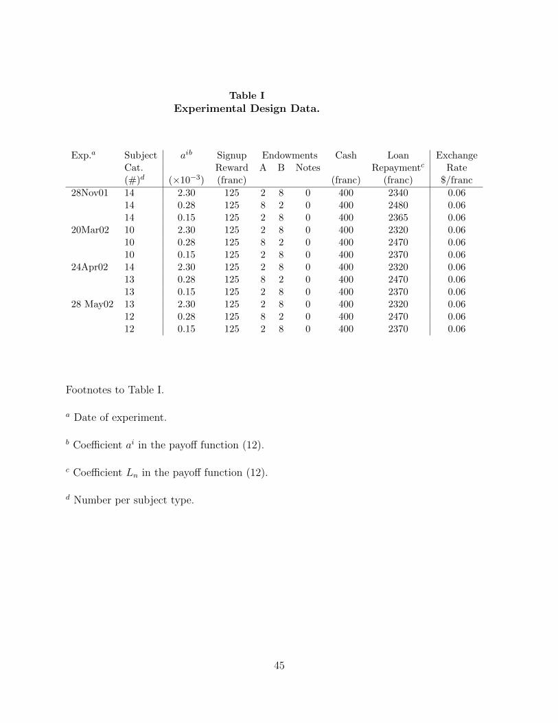
Table I
Experimental Design Data.
Exp.a Subject aib Signup Endowments Cash Loan ExchangeCat. Reward A B Notes Repaymentc Rate(#)d (×10−3) (franc) (franc) (franc) $/franc
28Nov01 14 2.30 125 2 8 0 400 2340 0.0614 0.28 125 8 2 0 400 2480 0.0614 0.15 125 2 8 0 400 2365 0.06
20Mar02 10 2.30 125 2 8 0 400 2320 0.0610 0.28 125 8 2 0 400 2470 0.0610 0.15 125 2 8 0 400 2370 0.06
24Apr02 14 2.30 125 2 8 0 400 2320 0.0613 0.28 125 8 2 0 400 2470 0.0613 0.15 125 2 8 0 400 2370 0.06
28 May02 13 2.30 125 2 8 0 400 2320 0.0612 0.28 125 8 2 0 400 2470 0.0612 0.15 125 2 8 0 400 2370 0.06
Footnotes to Table I.
a Date of experiment.
b Coefficient ai in the payoff function (12).
c Coefficient Ln in the payoff function (12).
d Number per subject type.
45

Table II
Projections Of Transaction Price Changes Onto Weighted Sum Of WalrasianExcess Demands
Exp. Periods Signa Security Coefficientsb R2 F -statisticc Id ρe
Intercept Excess DemandA B
28Nov01 1-4 − A 0.1 20.7 -6.5 0.05 27.0 1138 −0.12∗∗
(0.0) (2.8) (0.9) (< .01)B -0.0 -1.4 1.5 0.06 33.6 1138 -0.06
(0.0) (1.8) (0.6) (< .01)5-8 + A 0.6 20.0 5.4 0.05 31.3 1224 −0.30∗∗
(0.1) (2.8) (0.9) (< .01)B -0.1 0.5 1.2 0.05 30.3 1224 0.03
(0.1) (1.7) (0.5) (< .01)
20Mar02 1-4 + A 0.6 18.8 5.4 0.04 12.8 668 -0.02(0.1) (3.7) (1.1) (< .01)
B -0.5 -5.9 1.8 0.12 45.5 668 0.04(0.2) (4.6) (1.4) (< .01)
5-8 − A -0.3 32.1 -8.1 0.06 16.6 491 -0.07(0.1) (7.3) (2.5) (< .01)
B -0.0 -7.0 6.2 0.16 48.1 491 0.08(0.1) (5.0) (1.7) (< .01)
46

Table II
Projections Of Transaction Price Changes Onto Weighted Sum Of WalrasianExcess Demands (Continued)
Exp. Periods Signa Security Coefficientsb R2 F -statisticc Id ρe
Intercept Excess DemandA B
24Apr02 1-4 + A 1.3 33.6 10.1 0.07 26.5 745 −0.03(0.2) (4.6) (1.4) (< .01)
B -0.3 -2.2 0.5 0.07 25.9 745 0.06(0.1) (3.0) (0.9) (< .01)
5-8 − A -0.3 17.4 -5.2 0.04 14.4 675 -0.04(0.1) (5.2) (1.9) (< .01)
B 0.1 -31.9 12.6 0.14 52.6 675 -0.07(0.1) (3.6) (1.3) (< .01)
28May02 1-4 + A 0.6 18.8 4.9 0.04 18.4 825 0.04(0.2) (3.7) (1.2) (< .01)
B -0.8 10.5 6.9 0.16 76.5 825 0.04(0.2) (3.5) (1.1) (< .01)
5-8 − A -0.1 9.0 -2.9 0.02 4.3 563 −0.14∗∗
(0.1) (3.1) (1.1) (0.01)B -0.1 -9.3 4.6 0.08 23.6 563 0.01
(0.1) (3.4) (1.2) (< .01)
Footnotes to Table II.a Sign of the off-diagonal element of the matrix Ω. The OLS coefficient matrix evidently inheritsthe structure of this matrix.b OLS projections of transaction price changes onto (i) an intercept, (ii) the weighted sumof Walrasian excess demands for the two risky securities (A and B). Each individual excessdemand is weighted by the coefficient ai. Time advances whenever one of the three assetstrades. Boldfaced coefficients are significant at the 1% level using a one-sided test (effect ofown excess demand is positive; cross-effect has the same sign as the corresponding covariance).Standard errors in parentheses.c p-level in parentheses.d Number of observations.e Autocorrelation of the error term; ∗ and ∗∗ indicate significance at the 5% and 1% level,
respectively.
47

Table III
Mean Absolute Deviations Of Individual Portfolio Weights FromMarket Portfolio Weights
Experiment Periods Signa Period1 or 5 2 or 6 3 or 7 4 or 8
28Nov01 1-4 − 0.15b 0.14 0.12 0.12(0.02)c (0.02) (0.02) (0.02)
5-8 + 0.24 0.25 0.23 0.26(0.03) (0.03) (0.03) (0.03)
20Mar02 1-4 + 0.24 0.26 0.24 0.25(0.03) (0.03) (0.03) (0.03)
5-8 − 0.13 0.11 0.13 0.11(0.02) (0.02) (0.03) (0.02)
24Apr02 1-4 + 0.25 0.26 0.25 0.25(0.02) (0.02) (0.02) (0.03)
5-8 − 0.17 0.12 0.10 0.09(0.02) (0.01) (0.01) (0.01)
28May02 1-4 + 0.24 0.27 0.22 0.22(0.03) (0.02) (0.02) (0.03)
5-8 − 0.17 0.15 0.10 0.10(0.02) (0.02) (0.02) (0.02)
Footnotes to Table III.a Sign of the off-diagonal element of the matrix Ω. The mean absolute deviationof final holdings from per-capita average holdings is significantly larger whenthis sign is positive.b Average absolute difference between (i) the proportion individuals investin A relative to total franc investment in securities A and B, and (ii) thecorresponding weight in the per-capita holdings of A; weights are computedon the basis of end-of-period prices and holdings.c Standard error in parentheses.
48

0 1000 2000 3000 4000 5000 6000 7000 8000 9000160
180
200
220
240
28 Nov 01
0 1000 2000 3000 4000 5000 6000 7000 8000 9000160
180
200
220
240
20 Mar 02
0 1000 2000 3000 4000 5000 6000 7000 8000160
180
200
220
240
24 Apr 02
0 1000 2000 3000 4000 5000 6000 7000 8000160
180
200
220
240
28 May 02
Figure 1. Evolution of transaction prices of securities A [dashed line] and B [dash-dotted line].Horizontal lines indicate equilibrium price levels [A: solid line; B: dotted line]. Time (in seconds)on horizontal axis; prices (in francs) on vertical axis. Vertical lines delineate periods.
49
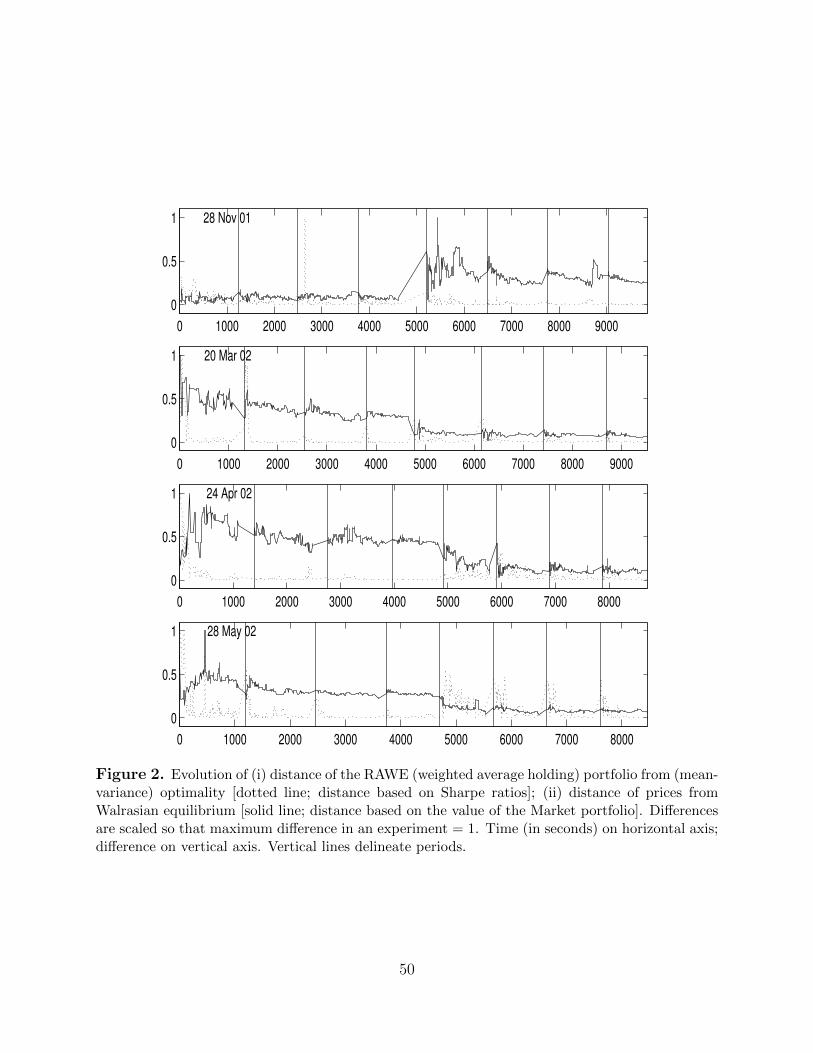
0 1000 2000 3000 4000 5000 6000 7000 8000 90000
0.5
1 28 Nov 01
0 1000 2000 3000 4000 5000 6000 7000 8000 90000
0.5
1 20 Mar 02
0 1000 2000 3000 4000 5000 6000 7000 80000
0.5
1 24 Apr 02
0 1000 2000 3000 4000 5000 6000 7000 80000
0.5
1 28 May 02
Figure 2. Evolution of (i) distance of the RAWE (weighted average holding) portfolio from (mean-variance) optimality [dotted line; distance based on Sharpe ratios]; (ii) distance of prices fromWalrasian equilibrium [solid line; distance based on the value of the Market portfolio]. Differencesare scaled so that maximum difference in an experiment = 1. Time (in seconds) on horizontal axis;difference on vertical axis. Vertical lines delineate periods.
50

Notes
∗Asparouhova is from the University of Utah, Bossaerts is from the University of Mel-
bourne, and Ledyard is from the California Institute of Technology. We would like to thank
Bernard Cornet for pointing out a mistake in an earlier draft. We gratefully acknowledge
comments on prior versions from participants in seminars (Bocconi, UBC, Copenhagen Busi-
ness School, Columbia University, U of Geneva, Hewbrew University, U of Lausanne, U of
Michigan, NYSE, New University in Lisbon, Norwegian Business School, Norwegian School
of Economics and Business Administration, SEC, Stanford, SIFR, Tel Aviv University, UC
Berkeley, UC Irvine, UC San Diego, U of Kansas, U of Vienna, U of Zurich) and confer-
ences (2003 ESA meetings, 2003 WFAs, 2003 and 2009 SAET, 2004 Kyoto Conference on
Experiments in Economic Sciences, 2005 Princeton Conference on Econometrics and Exper-
imental Economics, 2005 Purdue Conference in honor of Roko Aliprantis, 2006 Decentral-
ization Conference in Paris). We acknowledge the support from NSF grant SES-0527491
(Bossaerts, Ledyard), SES-0616431 (Bossaerts), SES-106184 (Asparouhova, Bossaerts), and
the Swiss Finance Institute (Bossaerts). Some of the experimental results have previously
been circulated in a working paper ”Equilibration Under Competition In Smalls: Theory
and Experimental Evidence.”.
1Under Pareto optimality, it is impossible to re-arrange allocations such that at least one
individual is better off, and nobody is worse off.
2Among the influential models have been those of Bansal and Yaron (2004), Campbell
and Cochrane (1999), and Epstein and Zin (1989). An up-to-date review of those models
can be found in Cochrane (2016).
3In the special case of investor preferences that generate the CAPM equilibrium, the
conditions of convergence to the optimal and the equilibrium resting points coincide.
51

4With generic preferences, the construct of a representative investor exists if and only if
allocations are optimal. This means that the equilibrium pricing relationships would hold
as long as an optimal allocation is achieved, even if this allocation is not the equilibrium
under the original initial endowments. In this sense, any rejection of an asset pricing theory
is very powerful as it not only rejects that the markets are in equilibrium but it also rejects
that the markets have achieved an optimal allocation under the assumed preferences.
5In light of the recent work of Budish, Cramton, and Shim (2015), an intermittent call
market, or a “frequent batch auction” market desing shoud also fall into the category of
market institutions for which our theoretical treatment applies.
6See Leijonhufvud (2006) for an illuminating discussion about the “methamorphosis of
neoclasicism.” Relevant for our motivation and discussion is his observation that “In the
early decades of the twentieth century, all economists distinguished between statics and
dynamics. By “dynamics,” they did not mean intertemporal choices or equilibria but instead
the adaptive processes that were thought to converge on the states analyzed in static theory.
[...] The conceptual issues that divide old and modern neoclassical theory are both numerous
and important. [...] If observed behavior is to be interpreted as reflecting optimal choices,
one is forced to assume that economic agents know their opportunity sets in all potentially
relevant dimensions. If this is true for all, the system must be in equilibrium always.”
7The paper provides a summary of empirical evidence and develops a model of firm
optimization in such an environment. We thank Sean Crockett for pointing us to this study.
8Samuelson provides a formalization of this based on the inverses of the partial equilibrium
aggregate demand and supply curves. Unfortunately, in an exchange economy there is no
obvious way to generate an inverse demand function or an inverse supply function without
making some explicit assumptions about the allocations that do not seem reasonable. If we
assume there are only two goods and quasi-linear utility functions, then di(p) = ∇xu−1(p)−
wi. We can say the aggregate demand at p is D(p) =∑
i max0, di(p) and the supply
is S(p) = −∑
i min0, di(p). Given D(p) the “demand price” is D−1(Q). The dynamic
52

proposed by Samuelson is dQ/dt = α[D−1(Q) − S−1(Q)]. Left unsaid is what happens to
each di.
9We will call this a bid but it could also be i’s “reserve price” where they would be willing
to take a unit of k in trade at a price lower than bik,t if they saw such a price offered in the
market.
10See the Section C in the Appendix for one possible calculation of “too large”.
11Another way to see whether (1)-(4) might describe something real is to consider whether
it is incentive compatible. Would an optimizing agent be willing to follow these rules? It
can be shown that (1)-(4) satisfies two types of incentive compatibility.
Suppose i believes (1) and that q is unknown. If i wants to protect herself against
possible losses, i.e. i wants to ensure that ∆ui = ui(xi(t) + ∆xi(t)) − ui(xi(t)) ≥ 0, then i
should choose bi = ρi. So i should choose ci = 1/τ. This type of local incentive compatibility
is identical to that introduced by Dreze and de la Valllee Poussin (1971). It is a maximin
type of defensive bidding which exhibits extreme risk aversion.
One can also imagine a less defensive approach. Suppose all i believe ∆ri = α(bi − q)
and that q = (1/I)∑bi, the Marshallian equilibrium price. Further suppose they choose bi
to be a local Nash Equilibrium. That is, for every i,
bi ∈ argmax ∆ui = (ρi − q)α(bi − q) (1)
= (ρi −∑
j bj
I)(bi −
∑j b
j
I) (2)
Letting b =∑bj
I, the first order conditions for this are: −1
I(bi − b) + I−1
I(ρi − b) = 0 or
bi = b + (I − 1)(ρi − b). Summing over i gives b = ρ =∑ρi
I. So the local Nash equilibrium
has bi = ρ+ (I−1)(ρi− ρ). Since q = b = ρ this means bi = q+ (n−1)(ρi− q). Compare this
to (2) to see that ci = I−1τ
. Thus, local Nash equilibria look exactly like local Marshallian
equilibria.
53

12If one thinks of the local Walrasian model with F i = ηi|||ηi|| ≤ R then the local
Walrasian demand is ci(ρi − q). So one can interpret (11) as indicating that prices adjust
proportionally to local excess demands. That is, (10) and (11) are the local equivalent of
the global non-tatonnement model from Section 2.
13Condition (ii) is included above for technical reasons. If dui/dt ≥ 0 along the path for
all i, then (ii) wouldn’t be necessary. But when dui/dt < 0 is possible for some i, we need to
worry about x(t) hitting the boundary of the feasible consumption set. There are standard
ways to modify (11) to deal with this. We do not pursue them here.
Condition (i) is included because we do not have a proof of convergence for utilities with
income effects. Indeed, we believe it would be relatively easy to construct examples where
such convergence will not occur. One could, of course, revise the model and impose a No
Speculation condition on trades that would ensure dui/dt ≥ 0. We do not do that here
largely because, as we will see below, the model as it now stands is consistent with the data.
14This way, subjects with knowledge of general equilibrium theory could not possibly
compute equilibrium prices. Specifically, subjects could not form reasonably credible expec-
tations about where prices would tend to.
15The prices of the Notes are not shown; these are invariably close to 100 francs, their
no-arbitrage value.
16We also ran projections with unweighted average Walrasian excess demands, and the
results are qualitatively the same.
17They compare the null hypothesis that the coefficient is zero against the alternative that
it is positive (in the case of the projection coefficient of a security’s own aggregate excess
demand) or has the same sign as the off-diagonal elements of Ω (in the case of the projection
coefficient of the other security’s aggregate excess demand).
54

18These results replicate the findings in Asparouhova, Bossaerts and Plott (2003) and
Asparouhova and Bossaerts (2009). There, quadratic preferences were indirectly induced,
through risk. In Asparouhova, Bossaerts and Plott (2003), there were two risky securites;
in Asparouhova and Bossaerts (2009), there were three. The latter setting is particularly
illuminating: Asparouhova and Bossaerts (2009) reports that the partial correlation between
changes in prices of an asset and the Walrasian excess demand of another asset reflects the
magnitude and sign of the corresponding element of the payoff covariance matrix.
19Note that CAPM pricing is a sufficient but not a necessary condition for the difference
measure to be zero.
20Arrow and Hahn (1971), p. 263.
21There are a variety of generalizations of this structure that allow for variations in the
speed of adjustment such as dpk/dt = λkek(p, ω) with λk > 0. We will not need to refer to
these in this paper.
22For specific examples of this type of dynamic, see Arrow and Hahn (1971), Hahn and
Negishi (1962), Uzawa (1962), Friedman (1979), and Friedman (1986).
23This might describe, for example, the “book building” process in a call market if orders
can be withdrawn. It should not be expected to describe the price formation process in a
continuous trading market in which transactions occur as prices are changing.
24They call this a Marginal Walrasian equilibrium.
25A discrete version of the Local Walrasian theory has been provided by Bonnisseau and
Nguenamadji (2009). The primary difference from the above is that they use the global
utility, ui(xi(t)+ηi), in place of the local utility, ∇ui(xi) ·ηi. With that, and the discreteness
of time, they get convergence to Pareto-optimal allocations in a finite number of steps.
55

26Note that this requires F (x(t)) to depend on q∗(t) and x∗(t) which is consistent with
the logic of the Appendix. But it means that “step size” and “equilibrium prices” are being
simultaneously determined.
27Note that this does require ci to depend on q∗(t) and x∗(t). But that is consistent with
the model in the Appendix.
56
Related Documents


