Competition and horizontal integration in maritime freight transport

Competition and horizontal

integration in maritime

freight transport

>Pedro Cantos Sanchez

Universitat de València and ERI-CES, Spain

>Rafael Moner-Colonques


>Jose Sempere-Monerris


>Oscar Alvarez

Universitat de València and IEI, Spain

June, 2010

DPEB

07/10

Competition and horizontal integration inmaritime freight transport!

Pedro Cantos-Sanchez1, Rafael Moner-Colonques2, Jose Sempere-Monerris3 and Óscar

Alvarez4

1,2,3 Department of Economic Analysis and ERI-CES, University of Valencia, Campus

dels Tarongers, Avd. dels Tarongers s/n, 46022 Valencia, Spain (e-mail corresponding

author: [email protected])4 Department of Economic Analysis and IEI, University of Valencia, Campus dels Tarongers,

Avd. dels Tarongers s/n, 46022 Valencia, Spain

Abstract. This paper develops a theoretical model for freight transport characterized by

competition between means of transport (the road and maritime sectors), where modes are

perceived as di!erentiated products. Competitive behavior is assumed in the road freight

sector, and there are constant returns to scale. In contrast, the freight maritime sector is

characterized by oligopolistic behavior, where shipping lines enjoy economies of scale. The

market equilibrium where the shipping lines behave as prot maximizers, provides a rst

approximation to the determinants of market shares, prots, and user welfare. We then

characterize the equilibrium when horizontal integration of shipping lines occurs, with

and without further economies of scale. An empirical application to the routes Valencia-

Antwerp and Valencia-Genoa uncovers that the joint prot of the merged rms and social

welfare always increase. However, user surplus only increases when economies of scale are

signicantly exploited.

Keywords: freight transport, shipping lines, horizontal integration..

!We gratefully acknowledge nancial support from CEDEX, Ministry of Works, under project PT-2007-

027-01CAPM.

1 Introduction

Total road freight transport in Europe is expected to grow by about 60% by 2013. This

growth would suppose an increase in the negative externalities caused by congestion, ac-

cidents, and environmental damage. Consequently, alternative modes to road transport

should be used more intensively than hitherto. In fact, seaborne trade in merchandise

goods, mainly carried by liner shipping, reached 29.1 trillion ton-miles by 2005. The

development of container shipping has certainly contributed to the increase in maritime

tra"c, a market with a small number of big shipping lines. The objective of this paper

is to develop a freight transport model characterized by competition between road and

maritime transport; the model accounts for product di!erentiation between the two modes

and for economies of scale in the shipping line market.

The liner shipping market has a number of characteristics, of which the following

stand out. First, there has been an increase in the size of rms and the emergence of

global carriers. The top 20 carriers accounted for 71% of vessel capacity deployed in 2005.

Second, mergers and cooperation agreements have been common in the past few years.

Since the 90s, the formation of strategic alliances permits carriers to pool vessels on main

commercial routes and prot from scope and network economies. Third, organising the

transport of freight by sea involves a number of di!erent agents: freight forwarders, port

actors (cargo handlers, stevedores, and shipping agents), shipping companies and inland

transport providers. Containerization has paved the way not only to horizontal integration

but also to vertical integration in an e!ort to improve the management of logistics chains.

Vertical integration can help companies to reap the benets of intermodal transport. De-

spite the increase in this type of structural moves, the biggest shipping lines remain the

key actors in transport chains. Fourth, the liner shipping industry exhibits economies of

scale, related to the size of the rm as well as to trade density. Fifth, shipping lines are

recently becoming more interested in the hinterland transportation sector. The door-to-

door service feature acknowledges the relevance of the combination of several transport

modes (sea, road, railroad) in the provision of a good service, which means not looking at

other transport modes only as competitors.

The model that we propose assumes competition for freight transport between the

road and the maritime sectors and captures quite a number of the features that char-

acterize the liner shipping market. In particular, we consider a route with two shipping

companies where road transport is supplied competitively. The services o!ered by opera-

tors are perceived as di!erentiated by shippers. The road transport sector does marginal

1

cost pricing whereas the shipping companies hold market power and enjoy economies of

scale1. We begin by characterizing the equilibrium in this market environment. Results

can be intuitively presented in terms of parameters related with product di!erentiation

and with the size of economies of scale. Then we study the e!ects on fares and market

shares when the shipping lines merge (horizontal integration). This is done under two

possible scenarios, one with and one without any cost gains. The model is then applied

to the route Valencia-Genoa, where Bulcom Intramed Service and Turkon Container Line

are the two maritime operators. We use information on travel volumes, price elasticities,

and estimates of costs to recover the unknown parameters in the demand functions. We

may then study the e!ects on tra"c distribution, prices, prots, and welfare levels under

a horizontal integration move.

There is an extensive literature that studies di!erent aspects of maritime transport.

The papers by Jansson and Shneerson (1985) and by Song et al. (2005) provide evi-

dence of economies of scale and of network economies, respectively. Heaver et al. (2000)

suggests that the extent and form of cooperative agreements, where shipping lines gure

prominently, has put them in an excellent negotiating position with port authorities. In

a sense, the shipping companies have become much stronger players relative to shippers,

stevedores and port authorities. Our model gives shipping lines a relevant role in a setting

with strategic price interaction and examines, theoretically and empirically, the e!ects of

horizontal integration. A game-theoretical approach has recently been undertaken by De

Borger et al. (2008), who study duopolistic pricing by ports and optimal investment poli-

cies in port and hinterland capacity. The recent paper by Cariou (2008) o!ers an overview

of the main trends in the liner shipping market during the last 15 years. The importance

of market power and the integration of activities in the maritime sector are made clear by

two recent OECD works by Frémont (2009) and Van de Voorde and Vanelslander (2009).

The main results can be summarized as follows. Whether maritime freight increases

after the merger is shown to depend on the existence of further economies of scale stemming

from the merger process. In case prices for maritime services increase, which occurs when

the merger only has strategic e!ect, road freight transport also increases. Furthermore,

under some conditions, horizontal integration is found to be benecial in private and social

terms. The next Section presents the model and theoretical results. Section 3 develops an

1Panayides (2003) studies the strategy-performance relationship in ship management nding that

achieving economies of scale and di!erentiation (through a wider range of services o!ered) have a strong

inuence on performance. The increased emphasis on such relationship is due, among other things, to

intense competition (as evidenced by the trend in cooperation already mentioned).

2

empirical application to the route Valencia-Genoa and Section 4 briey concludes.

2 The Model

Consider a connection between two regions, ! and ". This connection can be established

by two ways. The rst one is a long haul truck link, denoted by #$ that transports the

goods from ! to ", and the other is a combined transport mode in three legs, denoted

by %. The rst leg, a land leg, consists of a truck service delivering the goods from ! to

one port &!' Then, a second leg is sea transport which is delivered by two di!erentiated

shipping lines that carry the goods from port &! to port &" and nally a third land leg,

which consists of a truck service delivering the goods from &" to ".2 Suppose that users

of this transport system consider the two modes # and % as substitutes and also consider

as di!erentiated the services provided by the two shipping lines, denoted by %1 and %2. In

this way we model the demand for transport as a system of three linear demand functions

as follows:

(# = )# " *# + +(*$1 + *$2)

($1 = )$ " *$1 + +(*# + *$2) (1)

($2 = )$ " *$2 + +(*$1 + *#)

where (% is the demand (expressed in Tn-km) corresponding to service ,, for , = #$

%1$ %2$ also -% corresponds with the maximum level of transport demand for transport

mode , and nally, *% is the total price for each mode. In particular, .# is the truck

fare per Tn-km, so that *$& , / = 1$ 2 is the sum of the truck fares for the rst and third

legs, .#' and .#( respectively, and the shipping line fares also in Tn-km, .$&$ / = 1$ 2. We

next assume that the truck industries either the long haul or the other two that provide

shorter land services are competitive industries in the sense that the equilibrium price is

the competitive price, while the shipping line industry is a duopoly that sets prices in a

strategic way. Denote by 0#, #' and #( the corresponding marginal costs of the long haul,

truck ) and truck 1 industries. By the above assumption, *# = .# = 0#$ *$1 = #' + #( + .$1

and *$2 = #'+ #(+ .$2$ thus we can reformulate the above demand system by dening the

constant terms as follows: -# = )# + 2+(#' + #()$ and -$1 = -$2 = )$ " (1 " +)(#' + #()'

Further note that the system of demand equations must satisfy the condition saying that

an increase in the same amount of all prices must imply a decrease in demand; thus +

must be smaller than 12 ' Regarding the shipping line industry, we assume the following cost

2Roughly speaking, a maritime logistics chain consists of three large sections, the purely maritime

activities, goods handling in the port and hinterland transport services. Our model accounts for two of

them.

3

functions: 2$&(($&) = 0&($& " )2 (2$&$ with 0& and 3 4 0$ for / = 1$ 2$ which exhibit increasing

returns to scale.3 Thus, the extent of the returns to scale is parameterized by 3$ and is

assumed that marginal cost are positive, that is ($& 5*!) for all /'

We are interested in nding the equilibrium prices, user surplus and social welfare of

the transport system and compare this equilibrium with the case where a merger takes

place in the shipping line industry, that is, after a horizontal integration move.

i) Initial situation equilibrium

Each shipping company chooses the prot maximizing price, so that shipping line /

maximizes !$& = .$&($& " 0&($& + )2 (2$&' Computing the two rst order conditions we reach

the following system of equilibrium conditions (!$& =+!"!"*!1") / = 1$ 2 and .!# = 0#$ obtaining

the following equilibrium prices:

.!$& = (1"3)µ2(-# + +0#)" (1" +)(01 + 02) + (1 + +)(0, " 0&)

2(1 + (1" 3)(1" +))

¶+0&$ for /$ 6 = 1$ 2 and / 6= 6'

Note that if 02 4 01 then (!$2(01$ 02) 5 (!$1(01$ 02)$ and (!$1 #

*1) for nonnegative marginal

costs. At equilibrium.

(!# (01$ 02) = (-# " 0# + +(01 + 02)) + +(1" 3)((!$1 + (!$2)$

!!# (01$ 02) = 0$ !!$&(01$ 02) = (2" 32

)((!$&)2$ $/ = 1$ 2;

78!(01$ 02) =((!# )

2 + ((!$1)2 + ((!$2)

2

2$

89 !(01$ 02) =((!# )

2 + (3" 3) ((!$1)2 + (3" 3) ((!$2)

2

2'

The second order condition for a maximum imposes that 3 5 2$ while stability of

equilibrium requires that 0 5 + 5 2")1") $ which is a more binding condition on 3$ since +

cannot be negative. Therefore we assume that 3 5 1'

ii) Horizontal merger: shipping lines 1 and 2 merge.

When both shipping lines decide to merge, several post-merger situations can be

reached depending on the way the merger is capable of integrating the former separated

production processes. In one of the situations, the new entity sets prices to maximize prof-

its but both cost functions remain separate. In another, the merger can also internalize

the returns to scale due to the joint provision of products ($1 and ($2. In fact, the new

entity might even prot from synergies that meaning that the post-merger cost function

parameters would change so that 00: would be smaller or 3 higher or both things. In

the literature of horizontal mergers, the rst situation is usually associated with the case

where the merger only has strategic e!ects by the internalization of competition among3A linear marginal cost function reecting increasing returns to scale or tra"c density has been employed

by Brueckner and Spiller (1991). Constant returns correspond to ! = 0.

4

shipping line companies. The second situation comprises both a strategic e!ect and also

an e"ciency gain due to further exploitation of scale economies, whereas the third case

also implies more e"ciency because of cost improvements. In this subsection, we will

consider the case of symmetric shipping lines, i. e. 01 = 02 = 0. Note that the di!erence

between these approaches is easily modelled by looking at the following prot functions:

a) Post-merger situation a: !$1$2 = .$1($1 + .$2($2 " 0(($1 + ($2) + )2 ((

2$1 + (

2$2)

b) Post-merger situation b: !$1$2 = .$1($1 + .$2($2 " 0(($1 + ($2) + )2 (($1 + ($2)

2

c) Post-merger situation c: !$1$2 = .$1($1 + .$2($2 " 0̄(($1 + ($2) + )̄2 (($1 + ($2)

2$ with

0̄ # 0 and/or 3 5 3̄'

We will only consider situations ) and 1'

-Situation a (without further economies of scale).

The new entity chooses the pair of prices (.$1$ .$2) to maximize !$1$2 = .$1($1+.$2($2"

0(($1 + ($2) +)2 ((

2$1 + (

2$2)' Then, solving the system formed by -!"1"2

-+"1= 0 and -!"1"2

-+"2= 0$

we get that ('$1 = ('$2 = ('$ =+#" "*

( 11"$"))

4. Noting that .'# = 0# we obtain the equilibrium

prices .'$ = (1

(1".) "3)((/%+.*%)"(1".)*)

(2"(1".))) + 0' At equilibrium the other relevant variables are

given by:

('# = (-# " 0# + 2+0) + 2+(1

(1" +)" 3)('$ $

!'$1$2 = 2(.'$ " 0) (('$ ) + 3 ((

'$ )2 = (

2

(1" +)" 3) (('$ )

2 $

78' =(('# )

2

2+ (('$ )

2 $

89 ' =(('# )

2

2+ (

2

(1" +)+ (1" 3)) (('$ )

2 '

-Situation b (with further economies of scale).

The new entity chooses the pair of prices (.$1$ .$2) to maximize !$1$2 = .$1($1+.$2($2"

0(($1 + ($2) +)2 (($1 + ($2)

2' Then, solving for -!"1"2-+"1

= 0 and -!"1"2-+"1

= 0$ we get, for the

symmetric cost case, that (($1 = (($2 = (($ =+&""*

( 11"$"2))

5. As above noting that .(# = 0#,

the equilibrium shipping prices .($ = (1

(1".) " 23)((/%+.*%)"(1".)*)2(1"(1".))) + 0' The other relevant

4Global second order conditions are satised for ! " 1# since ! " 1 " 21+$2

# which implies that the

determinant of the Hessian matrix is positive.5As above global second order conditions are satised for ! " 1# since ! " 1 " 2

(1"$)2 # and the

corresponding determinant of the Hessian matrix is positive as ! " 1 " 1(1"$) .

5

variables are given by:

((# = (-# " 0# + 2+0) + 2+(1

(1" +)" 23)(($ $

!($1$2 = 2(.($ " 0)³(($

´+ 23

³(($

´2= 2(

1

(1" +)" 3)

³(($

´2$

78( =

¡((#¢2

2+³(($

´2$

89 ( =

¡((#¢2

2+ (

2

(1" +)+ (1" 23))

³(($

´2'

Some Results

We are rst interested in nding how shipping tra"c evolves after one of the proposed

merger situations occurs. It is easy to prove the next result for the symmetric case 01 =

02 = 0.

Result 1 : Either ('$ 5 (($ 5 (

!$ if 3 % (0$

.1+. ),or (

'$ 5 (

!$ 5 (

($ if 3 % (

.1+. $ 1)'

The proof is straightforward just noting that (!$ =(/%+.*%)"(1".)*1+(1".)(1")) $ (

'$ =

(/%+.*%)"(1".)*(2"(1".)))

and (($ =(/%+.*%)"(1".)*2(1"(1".))) $ then the ranking holds for 0 5 3 5 1$ 0 5 + 5 1

2 ' The merger with

only strategic e!ect internalizes the competition among the shipping lines thus implying

a positive marginal prot at the pre-merger equilibrium price. Thus a higher price is

attained at the post-merger equilibrium and then output falls. Alternatively, if the merger

incorporates further scale e!ects then the marginal prot after the merger includes a new

negative term that induces post-merger equilibrium prices to fall in case it dominates the

previous positive e!ect, i.e. if 3 4 .1+. $ so that total output increases.

Note that for each merger situation to happen we need to ensure that it is privately

protable and also that the new entity nds it protable to keep both di!erentiated services

operative. Private protability is ensured as long as 2!!$&(01$ 02) 5 !'$1$2 and 2!

!$&(01$ 02) 5

!($1$2' The next result ensures that both merger types are privately protable for 01 = 02 =

0 :

Result 2: 2!!$&(0$ 0) 5 !'$1$2 5 !

($1$2'

The proof is also straightforward. Just note that the merger with only strategic e!ects

implies less output as compared with the initial situation, but the increase in market power

is enough to outweigh the output reduction with an increase in the margin thus leading

to greater prots. The merger with a better use of scale economies is even more protable

since it yields both an output and a margin increase at equilibrium. Also note that since

the long haul truck transport is a competitive industry, Result 2 proves that any of the

two types of merger increases rms’ prots.

6

The next feature to evaluate is how the long haul tra"c varies as a function of the

shipping line market structure.

Result 3: a) ('# is greater than both (!# and (

(# ' b) (

(# is greater than (

!# if and only if

0 5 3 5 12(1".)}$ otherwise (

!# is greater than (

(# $ with + 5

12 $ and 3 5 1'

Since the long haul truck industry behaves in a competitive way, prices are not reacting

to the varying pricing conditions in the shipping line industry. Thus, nal long haul

output for each shipping line market structure is fully explained by the shipping line

prices. Therefore, the greater the equilibrium shipping line prices the higher the long haul

output. Since prices are higher in the merger with only strategic e!ects as compared to

both the initial situation and the merger with further scale economies, then a merger with

only strategic e!ects implies the higher level of truck transport. Whether the merger with

further economies of scale implies higher level of truck transport than the one in the initial

situation depends on either low 3 or high +.

Result 4: A su"cient condition for 89 ( 4 89 ! to hold is .1". 5 3 and 3 5

min{ 2.1". $

12(1".))' Similarly a su"cient condition for 78

( 4 78! is .1". 5 3 5 1

2(1".) '

The above result, which is directly obtained from Results 1 and 3, indicates that for

low levels of scale economies the merger with further economies of scale can generate an

increase in the equilibrium of both the maritime transport and long haul truck transport.

This is enough to lead to an increase in user and social surplus. Remind, 3 5 12(1".)

implies ((# 4 (!# $ and.1". 5 3 implies (($ 4 (!$ ' The consideration of 3 5

2.1". has to do

with the comparison between the second terms in the respective social welfare functions,

( 2(1".)+(1"23))

¡(($¢2and (3"3) ((!$ )

2 ' If 3 5 2.1". $ then (2+(1"+)(1"23)) 4 (3"3)(1"+)'

Result 5: A su"cient condition for 89 ' 4 89 ! is 3 5 "(+)$ where "(+) increases in

+$ "(+ = 0'3907570) = 0' and "(+ = 12) = 1'

The precise expression for"(+) is "2+.(5+9."4.2)"&4"20.+53.2"70.3+41.4+8.5+16.68(1".).2 ' Re-

sult 5 indicates that low levels of scale economies together with high cross elasticities imply

that the increase in the long haul transport induced by the merger more than compen-

sates the reduction in maritime transport so that aggregate user welfare increases and since

rms’ prots also increase, total welfare goes in the same direction. Finally and consider-

ing a symmetric situation in the sense that -# = -$ and 0# = 0$ we provide the necesary

and su"cient condidions for 89 ' exceeds 89 !' In particular, for 0 5 3 5 #(+), where

#(+) is an increasing function in +$ #(+ = 0'251221) = 0 and #(+ = 12) = 0'347296' Note

that #(+) = "2+.(13"."2.2)"&4"20.+53.2"74.3+53.4+12.5+4.64(1".).2 ' Given that, if + 5 0'251221$

then 89 ' 5 89 ! for all 3 while if + 4 0'347296$ then 89 ' 4 89 ! for all 3'

7

3 Empirical application

In this section we are going to calibrate the theoretical model using actual data from

two particular routes between the Spanish port of Valencia and the ports of Antwerp and

Genoa. In boths routes there are two shipping lines which o!er maritime freight transport

between the two ports, and both services are di!erentiated. The average capacity is

slightly di!erent, and more importantly, the frequency of the two companies for each

route is di!erent as well. Besides we also have data about road tra"c supplied by trucking

companies between the region of Valencia (Spain) and the region of Flandre (Belgium) and

the region of Liguria (Italy), respectively. In particular, the number of Tons transported

by road and by each shipping line in 2007 were the following:

[Insert Table 1 about here]

Regarding costs, the truck industry costs can be calculated from o"cial data obtained

from “Observatorio del coste del transporte de mercancías por carretera 2008, Ministry of

Works”. Specically, the cost per vehicle km of a standard truck (carrying a 20 Tn capacity

container) is estimated to be 0.9 !. We do not have any available data on maritime costs,

but we provide information about the average shipping prices for sending a 20 Tn container

between the ports of Valencia-Antwerp and Valencia-Genoa. This average price can be

obtained from an electronic simulator, a public program provided by the Spanish Ministry

of Works. Then the parameters 0 and 3 in the cost equation are calibrated in order to

obtain equilibrium prices similar to those provided by the simulator. The nal values used

for 0 and 3 are 0.55 and 0.1! per 20 Tn container km, respectively.

Finally, we need estimates for the own and cross-price elasticities. In the calibration

we will consider di!erent elasticities for road and shipping transport, and therefore, we

will obtain values for the parameters in the demand expressions above. We employ the

data from the paper by Beuthe et al (2001):

[Insert Table 2 about here]

With all these data, the calibration follows a two stage process:

1. We rst identify the demand elasticities in the following asymmetric system: (# =

-̄# " ;#.# + +̄(.$1 + .$2)$ ($1 = -̄$1 " ;$.$1 + +̄(.# + .$2)$ ($2 = -̄$2 " ;$.$2 + +̄(.$1 + .#).

Note that the model developed has assumed, for simplicity, symmetry in own e!ects and

next a normalization of the coe"cents so that the coe"cients of prices are 1 and +'

By expressing quantities and prices in logarithms, the coe"cients are the values of the

elasticities. Therefore, a system of three equations with three unknowns can be solved to

obtain the values of ;#$ ;$ and +.

8

2. In the next step, values for -̄#$ -̄$1 and -̄$2 are calibrated. To do so, we take the

equilibrium expressions for quantities in the initial case and set them equal to the values of

20 Tn Container km transported (in logs). We can then solve a system of three equations

to estimate a value for -̄#$ -̄$1 and -̄$2.

With all these calibrated values we can obtain prices and quantities in logarithm, which

can be appropriately transformed in levels of ! per container km and thousands of con-

tainers km. We can also calculate the results for the di!erent scenarios. Table 3 column 1

reports the results for the initial case, whereas columns 2 and 3 report the results under

horizontal merger without and with further economies of scale.

[Insert Tables 3 and 4 about here]

Firstly, we are going to comment the results for the route Valencia-Antwerp. In table 3,

3 = 0'1 stands for the situation where economies of scale are very important. In the event

of merger, this parameter represents around one third of total costs saving. We also assume

that < = 0'6, thus considering that services are weakly di!erentiated. Regarding the two

types of merger, prices increase and the aggregate prots of the merged shipping lines are

higher than the sum of prots before merger; the rms always have strong incentives to

merge. We also obtain that consumer surplus and social welfare are maximal in the merger

with no economies. This outcome is explained by the strong increase in freight tra"c of

the competitive trucking sector. Finally, using data from INFRAS/IWW (2004), we can

estimate the negative externalities provoked by road and maritime freight transport. The

net social welfare, taking into account these estimates are reported in the last row.6 When

3 = 0'01 (see table 4 where 3 now represents a cost saving of 3.33% in the merger situation)

the results in terms of prices and tra"c levels change slighlty as compared with table 3,

and therefore, the social gains of the merger (without and with further economies) are

always signicant.

However, when < = 0'075 (see tables 5 and 6), this meaning that servicies between

road and shipping are clearly more di!erentiated, the changes in prices and tra"c levels

are very small with respect to the pre-merger scenario. Now the social gains from the

merger are lower, and again these gains are, as expected, more relevant when the shipping

lines can better exploit their economies of scale. Social welfare in the pre-merger regime

and the merger regime without further economies are now very similar in tables 5 and 6.

6We have considered that the average externality cost transported by a 20 Tn truck container is 1.42

! per km. The same number of tons transported by shipping lines supposes 0.45 ! per km.

9

[Insert Tables 5 and 6 about here]

Secondly, regarding the second route, Valencia-Genoa, the results are qualitatively

similar to those obtained for the route Valencia-Antwerp (see tables 7 to 10). Again the

social gains are higher in the merger scenarios when the services provided by road and

shipping lines are less di!erentiated. Summing up, we can conclude that product di!en-

tiation (approximated by the parameter of cross elasticity) seems more relevant in our

results than the parameter of economies of scale.

[Insert Tables 7 to 10 about here]

4 Conclusions

We have developed a theoretical model where the maritime sector, assumed oligopolistic,

competes for freight transport with a competitive road transport industry. Attention is

drawn to product di!erentiation and the size of economies of scale in the characterization

of market equilibrium without and with horizontal integration between shipping lines. It is

shown that maritime freight increases after the merger in case it entails further economies

of scale. In case prices for maritime services increase, which occurs when the merger

only has a strategic e!ect, road freight transport also increases. Furthermore, under some

conditions, horizontal integration is found to be benecial in private and social terms.

In the empirical application we have employed data for two freight routes between the

hinterland of Valencia and the hinterlands of Genoa and Antwerp. The results show that,

in all cases examined, the shipping lines have strong incentives to merge. Additionally, a

merger (horizontal integration) between two shipping lines where economies of scale are

further exploited generally leads to an increase in social welfare. Also, in most of the

cases, the merger produces a signicant increase in road tra"c, which is greater than the

reduction in tra"c transported by the shipping lines, and this fact leads to an increase in

user surplus. We have obtained that the social gains depend mainly of the characteristics

of the market. Then the social gains obtained with the merger are higher in those markets

where the road and shipping services are less di!erentiated. If the services are clearly

di!erentiated, then the social gains are signicantly lower.

There are many possible extensions that we wish to undertake in the future. It would be

interesting to analyze the situation if the trucking companies do not behave competitively.

Also we would like to study the possibility that lines can share the capacity of their

vessels, instead of supplying its own ones. Also it is interesting to consider asymmetric

costs, incorporating, for instance, economies in the size of the vessels. And nally, the

10

analysis of potential vertical integration, for example, between some trucking companies

and the shipping lines is another line of future research.

References

[1] Beuthe, M., B. Jourquin, J-F Geerts, C. Koul and N. Ha (2001). “Freight

transportation demand elasticities: a geographic multimodal transportation network

analyisis”. Transportation Research Part E 37, 253-266.

[2] Brueckner, J. K. and P. T. Spiller (1991). ‘Competition and Mergers in Airline

Networks’, International Journal of Industrial Organization, 9, 323—42.

[3] Cariou, P. (2008), Liner shipping strategies: an overview, International Journal of

Ocean Systems Management, 1, 2-13.

[4] De Borger, B., S. Proost and K. Van Dender (2008), “Private Port Pricing and

Public Investment in Port and Hinterland Capacity “, Journal of Transport Economics

and Policy, 42, 3, 527—561.

[5] Frémont, A., (2009), “Empirical evidence for integration and disintegration of

maritime shipping, port and logistics activities”, OECD/ITF Discussion paper 2009-

1.

[6] Heaver, T., H. Meersman, F. Moglia and E. Van de Voorde (2000), Do

mergers and alliances inuence European shipping and port competition?, Maritime

Policy and Management, 27, 4, 363-373.

[7] INFRAS/IWW (2004), "External Cost of Transport. Update Study. Final Report".

Zurich/Karlsruhe.

[8] Jansson, J.O. and D. Shneerson (1985), Economies of trade density in liner

shipping and optimal pricing, Journal of Transport Economics and Policy,

[9] Panayides, P. (2003), “Competitive strategies and organizational performance in

ship management”, Maritime Policy and Management, 30, 2, 123-140.

[10] Song, D., Zhang, J., Carter, J., Field, T, Marshall, J., Polak, J., Schu-

macher, K., Sinha-Ray, P. and J. Woods (2005), On cost-e"ciency of the

global container shipping network”, Maritime Policy and Management, 32, 1, 15-30.

[11] Van de Voorde, E. And Vanelslander, T. (2009), Market power and vertical

and horizontal integration in the maritime shipping and port industry, OECD/ITF

discussion paper 2009-2.

11

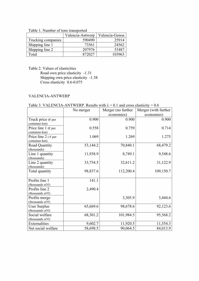
Table 1. Number of tons transported Valencia-Antwerp Valencia-Genoa Trucking companies 590490 25914Shipping line 1 73561 24562Shipping line 2 207976 53487Total 872027 103963 Table 2. Values of elasticities

Road own price elasticity -1.31 Shipping own price elasticity -1.38 Cross elasticity 0.6-0.075

VALENCIA-ANTWERP Table 3. VALENCIA-ANTWERP. Results with ! = 0.1 and cross elasticity = 0.6 No merger Merger (no further

economies) Merger (with further

economies) Truck price (€ per container-km)

0.900 0.900 0.900

Price line 1 (€ per container-km)

0.558 0.759 0.714

Price line 2 ( € per container-km)

1.069 1.269 1.275

Road Quantity (thousands)

53,144.2 70,840.1 68,479.2

Line 1 quantity (thousands)

11,938.9 8,749.1 9,548.6


33,754.5 32,611.2 31,122.9

Total quantity

98,837.6 112,200.4 109,150.7

Profits line 1 (thousands of €)

141.1


2,490.4

Profits merge (thousands of €)

3,305.9 3,444.6

User Surplus (thousands of €)

65,669.6 98,678.6 92,123.6

Social welfare (thousands of €)

68,301.2 101,984.5 95,568.2

Externalities 9,602.7 11,920.5 11,554.3Net social welfare 58,698.5 90,064.5 84,013.9

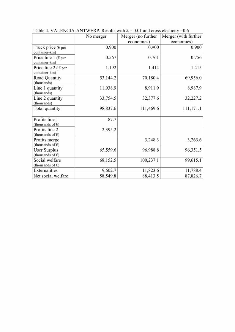
Table 4. VALENCIA-ANTWERP. Results with ! = 0.01 and cross elasticity =0.6 No merger Merger (no further



0.900 0.900 0.900


0.567 0.761 0.756


1.192 1.414 1.415


53,144.2 70,180.4 69,956.0


11,938.9 8,911.9 8,987.9


33,754.5 32,377.6 32,227.2

Total quantity

98,837.6 111,469.6 111,171.1


87.7


2,395.2


3,248.3 3,263.6


65,559.6 96.988.8 96,351.5


68,152.5 100,237.1 99,615.1


Table 5. VALENCIA-ANTWERP. Results with ! = 0.1 and cross elasticity = 0.075 No merger Merger (no further



0.900 0.900 0.900


0.559 0.574 0.538


1.069 1.075 1.061


53,144.2 53,275.5 52,966.2


11,938.9 11,499.6 12,577.4


33,754.5 33,575.9 33,961.2

Total quantity

98,837.6 98,351.0 99,504.8


141.1


2,490.3


2,645.1 3,038.8


15,527.8 15,500.0 15,563.3


18,159.9 18,145.1 18,602.1


Table 6. VALENCIA-ANTWERP. Results with ! = 0.01 and cross elasticity = 0.075 No merger Merger (no further



0.900 0.900 0.900


0.567 0.582 0.579


1.192 1.199 1.198


53,144.2 53,266.7 53,240.3


11,938.9 11,499.6 11,623.1


33,754.5 33,575.9 33,601.2

Total quantity

98,837.6 98,342.2 98,464.6


87.7


2,395.2


2,505.0 2,539.2


15,527.7 15,500.7 15,502.2


18,010.6 18,005.7 18,041.4


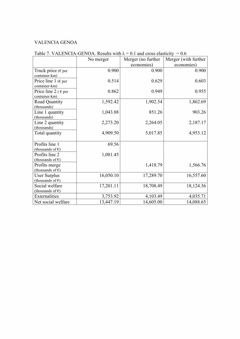
VALENCIA GENOA Table 7. VALENCIA-GENOA. Results with ! = 0.1 and cross elasticity = 0.6 No merger Merger (no further



0.900 0.900 0.900


0.514 0.629 0.603


0.862 0.949 0.955


1,592.42 1,902.54 1,862.69


1,043.88 851.26 903.26


2,273.20 2,264.05 2,187.17

Total quantity

4,909.50 5,017.85 4,953.12


69.56


1,081.45


1,418.79 1,566.76


16,050.10 17,289.70 16,557.60


17,201.11 18,708.49 18,124.36


Table 8. VALENCIA-GENOA. Results with ! = 0.01 and cross elasticity = 0.6 No merger Merger (no further



0.900 0.900 0.900


0.516 0.625 0.623


0.928 1.022 1.022


1,592.42 1,891.84 1,888.06


1,043.88 861.55 866.54


2,273.20 2,251.81 2,244.08

Total quantity

4,909.50 5,005.20 4,998.68


22.61


999.24


1,311.84 1,327.23


16,050.10 17,146.90 17,073.10


17,071.95 18,458.74 18,400.33


Table 9. VALENCIA-GENOA. Results with ! = 0.1 cross elasticity =0.075 No merger Merger (no further



0.900 0.900 0.900


0.514 0.523 0.513


0.835 0.837 0.833


1,592.42 1,594.85 1,589.11


1,043.88 1,017.78 1,081.35


2,273.20 2,270.43 2,275.07

Total quantity

4,909.50 4,838.06 4,945.53


68.67


1,020.12


1,097.62 1,322.35


3,256.85 3,235.63 3,284.96


4,345.65 4,333.25 4,607.31

Externalities 3,753.92 3,744.39 3,766.92Net social welfare 591.73 588.86 840.39

Table 10. VALENCIA-GENOA. Results with ! = 0.01 and cross elasticity =0.075 No merger Merger (no further



0.900 0.900 0.900


0.516 0.525 0.522


0.899 0.901 0.901


1,592.42 1,594.71 1,594.20


1,043.88 1,019.39 1,025.20


2,273.20 2,270.40 2,270.04

Total quantity

4,909.50 4,839.50 4,889.44


21.71


933.20


966.139 986.99


3,256.85 3,236.59 3,239.71


4,211.77 4,202.73 4,226.71

Externalities 3,753.92 3,744.89 3,746.63Net social welfare 457.85 457.83 480.08

Competition and horizontal integration in maritime freight transport

Documents