Competition amongst contests

Competition amongst Contests ∗

Ghazala Azmat †

andMarc Moller ‡

Abstract

This article analyses the allocation of prizes in contests. While existing mod-

els consider a single contest with an exogenously given set of players, in our

model several contests compete for participants. As a consequence, prizes not

only induce incentive effects but also participation effects. We show that contests

that aim to maximize players’ aggregate effort will award their entire prize bud-

get to the winner. In contrast, multiple prizes will be awarded in contests that

aim to maximize participation and the share of the prize budget awarded to the

winner increases in the contests’ randomness. We also provide empirical evidence

for this relationship using data from professional road running. In addition, we

show that prize structures might be used to screen between players of differing

ability.

JEL classification: D44, J31, D82.

Keywords: Contests, allocation of prizes, participation, incentives, screening

∗We are especially grateful to Michele Piccione and Alan Manning for their guidance and support.We also thank Jean–Pierre Benoit, Michael Bognanno, Jordi Blanes i Vidal, Pablo Casas–Arce, VicenteCunat, Maria–Angeles de Frutos, Christopher Harris, Nagore Iriberri, Belen Jerez, Michael Peters andparticipants at various seminars and conferences for valuable discussions and suggestions.

†Department of Economics and Business, University Pompeu Fabra, Ramon Trias Fargas 25-27,08005 Barcelona, Spain. Email: [email protected], Tel.: +34-93542-1757, Fax: +34-93542-1766.

‡Department of Economics, University Carlos III Madrid, Calle Madrid 126, 28903 Getafe Madrid,Spain. Email: [email protected], Tel.: +34-91624-5744, Fax: +34-91624-9329.

1

1 Introduction

The world is full of contests. In investment banks, financial analysts compete for

promotions; in architectural competitions, architects contend for design contracts; and

in sports contests, athletes compete for prize–money. How many hierarchical levels

should an investment bank implement? How should an architectural competition be

set up? And how should a sports contest distribute its prize–budget across ranks?

A recent literature has provided some answers to these type of questions by consid-

ering the implications of the design of a contest on the players’ incentives to exert effort.

A common assumption in this literature is that the set of players is given exogeneously.

However, as potential participants often have to choose between several contests, the

set of players itself might be influenced by the contest’s design. For example, an in-

vestment banker may decide to work for bank A rather than bank B because it offers

a steeper hierarchical structure and, in turn, a fast–tracking career. Due to differences

in contest rules, an architect may be reluctant to devote his time and effort to the

design proposal for the World Trade Center Site Memorial and instead participate in

the design competitions for the London 2012 Olympic Park. Similarly, a marathon

runner may enter the New York Marathon instead of the Chicago Marathon because it

awards a larger fraction of its prize money to suboptimal performances. In this paper

we study optimal contest design when contest designers have to provide contestants

with both, incentives to exert effort and incentives to participate.

Referring to the recent contests for European 3G telecom licenses, Paul Klemperer

(2002) notes that “a key determinant of success of the European telecom auctions was

how well their designs attracted entry [...]”. From the viewpoint of a contest designer,

attracting entry is important. Some contests benefit directly from the participation of

certain key–players or aim to maximize the total number of contestants. For example,

architectural competitions greatly benefit from the mere presence of prominent archi-

tects and big–city marathons boost their media interest by securing the participation

of elite runners.1 Other contests aim to maximize participants’ aggregate effort and

1In 2006 organizers of three major marathons went head to head in their bid for the world recordholder, Paula Radcliffe, and the U.S. record holder, Deena Castor (see “Marathons: Top Races areVying for the Elite Runners”, International Herald Tribune, June 12, 2006).

2

will benefit from entry indirectly through its positive effect on aggregate effort. In this

paper we study optimal contest design from both of these perspectives.

We consider a complete information model in which two contests compete for the

participation of a given set of N ≥ 3 risk–neutral players with linear costs of effort.

Players make their contest choice simultaneously and these choices depend of the con-

tests’ allocation of prizes. Once the set of participants has been determined in each

contest, players exert effort in order to win a prize. The contests’ outcome depends

on both, players’ efforts and the impact of exogenous factors (i.e., the level of ran-

domness). This level of randomness may vary substantially across different types of

contest. For example, while randomness plays a small role in a chess competition, it is

the main determinant in a poker tournament. Similarly the outcome of a labour market

tournament might be more random in industries characterized by high volatility, e.g.

the finanical market.

We begin our analysis by focusing on participation. We show that when organizers

aim to maximize participation, in equilibrium, contests will award multiple identical

prizes. We distinguish between three different types of contests: lotteries, where the

contests’ outcome is completely random; all pay auctions, where the contests’ outcome

depends only on effort; and imperfectly discriminating contests that depend on both,

randomness and effort. Our results are very general, i.e. they hold for an arbitrary

number of players, any number of prizes and easily generalize to models with more than

two contests. Overall, we find that the equilibrium number of prizes is decreasing in

the contests’ randomness. This implies that contests in which the impact of exogeneous

factors is more important will tend to offer a higher share of their prize budget to the

winner.

Using data from professional road running, we provide empirical evidence for this

relationship. We argue that as the race distance increases, the impact of exogeneous

factors on the race outcome becomes more important.2 We find that as the race

distance increases, there is a monotonic increase in the ratio between first and second

prize. For example, as the race moves from 5km to 42km, the ratio between the first

2While in a 5km race the prediction of the winner based on past performance turns out to becorrect in 43% of the cases, this number reduces to 20% for a marathon. For details see Section 6.

3

and the second prize increases by 4 percentage points. We find qualitatively similar

results when using alternative measures of competitiveness and after controlling for

various important factors.

When turning our attention to the maximization of players’ aggregate effort, we

find that awarding multiple prize rather than a single first prize has two effects. It

directly decreases effort for a given set of participants (incentive effect) and it indi-

rectly increases effort through its positive effect on participation (participation effect).

Under the assumptions of our model we show that the incentive effect outweighs the

participation effect. Hence when contest designers aim to maximize players’ aggregate

effort, in equilibrium contests will award their entire prize budget to the winner.

Our theory can provide an explanation for the significant differences in prize struc-

tures observed in reality. Contests that aim to maximize aggregate effort, as it is the

case in science and engineering competitions, are likely to implement the winner–takes–

all principle.3 In contrast, when participation itself is important, for example in sports

contests, multiple prizes will be awarded.

This paper also shows that prize structures might be used to screen players of

differing ability. When players are heterogeneous a contest might want to select the

most able players. We show that high ability players are more likely to enter contests

with steep prize structures than low ability players. This insight is especially important

in labour market settings where firms aim to attract the most productive workers.

It shows that firms with steep hierarchies can be expected to have a higher quality

workforce.

This paper is the first to model how contests compete for participants. The existing

literature on contest design has focused on single contests with an exogenously given

set of participants. In their seminal paper, Moldovanu and Sela (2001) show that the

optimal allocation of prizes depends critically on the shape of players’ cost of effort func-

tions. Multiple prizes become optimal when the costs of effort are sufficiently convex.

Multiple prizes have also been justified and derived from players’ risk aversion (Krishna

3The NASA 2007 Astronaut Glove Competition awards a single first prize of $250000 to the designerof the best performing glove. Similarly, the DARPA (Defense Advanced Research Projects Agency)2005 Grand Challenge awarded $2 million to the fastest driverless car on a 132–mile desert course.

4

and Morgan (1998)) and players’ heterogeneity (Szymanski and Valletti (2005)) but

under the restrictive assumption that the number of players is small (N ≤ 4). Other

papers provide arguments for the use of a single (Clark and Riis (1998b), Glazer and

Hassin (1988)) or large (Rosen (2001)) first prize or few prizes (Barut and Kovenock

(1998)). In addition, issues considered by this literature include simultaneous versus

sequential designs (Clark and Riis (1998a)), the splitting of a contest into sub–contests

(Moldovanu and Sela (2007)) and optimal seeding in elimination tournaments (Groh

et al. (2008)).

Although some papers endogenize the set of participants, they maintain the focus

on a single contest. Taylor (1995) and Fullerton and McAfee (1999), for example, study

how the set of participants, and hence the expected winning performance, in a research

tournament varies with its entry fee.

Competition for participants has attracted some attention in the literature on auc-

tion and mechanism design. McAfee (1993), Peters and Severinov (1997) and Burguet

and Sakovics (1999) for example, consider models in which auctions compete for bid-

ders. However, while in our model contests compete via their prize allocation, in these

papers, prizes are fixed and auctions compete by using their reservation price. More

related, Moldovanu et al. (2008) consider quantity competition between two auction

sites. Although their model is different in its setup it shares a common feature with

ours. In the same way in which in our model contests increase participation by award-

ing multiple prizes (at the cost of undermining incentives), in their model auctions

increase the number of bidders by raising their supply (at the cost of lowering prices).

Finally, the literature on labor tournaments is also relevant here. Lazear and Rosen

(1981), Green and Stokey (1983), Nalebuff and Stiglitz (1983), and Mookherjee (1984)

have shown that the introduction of some form of contest among workers could provide

optimal incentives to exert effort inside a firm. While Green and Stokey (1983) and

Mookherjee (1984) take the set of workers as exogenously given, Lazear and Rosen

(1981) and Nalebuff and Stiglitz (1983) assume a competitive labor market in which

each firm hires a fixed number of workers. While in these papers each worker faces

a fixed number of opponents, our results are driven by the fact that a player’s set of

opponents itself depends on the contest design.

5

The paper is organized as follows. In Section 2 we describe the theoretical model.

Section 3 considers the case where contest designers aim to maximize participation

while Section 4 contains our results about aggregate effort. In Section 5 we consider

the possibility of screening. Section 6 tests the predictions of Section 3 using data on

professional road running. Section 7 concludes. Some proofs and all empirical tables

are contained in the Appendix.

2 The model

We consider two contests, i ∈ {1, 2}, and N ≥ 3 players. Apart from possible dif-

ferences in the allocation of prizes, contests are homogeneous. We assume that con-

tests face the same budget V . Contests must choose how to distribute their budget

across ranks. In particular, contest i chooses a prize structure, i.e. a vector of non–

negative real numbers vi = (v1i , v

2i , . . . , v

Ni ) such that vm

i is (weakly) decreasing in m

and∑N

m=1 vmi = 1. The m’th prize awarded by contest i has the value vm

i V . Note

that in order to focus on the participation effects implied by a contest’s prize structure

we rule out the possibility that contests pay participants for attendance. Our results

remain valid when we allow for attendance pay (see discussion at the end of Section 3).

It will become clear that the contests’ competition in prize structures resembles price

competition a la Bertrand. As a consequence our results generalize to an arbitrary

number of contests.

In models with a single contest it has been shown that it may be optimal to award

second prizes when players are heterogeneous (Szymanski and Valletti (2005)), risk

averse (Krishna and Morgan (1998)), or have convex costs of effort (Moldovanu and

Sela (2001)). In order to identify competition for participants as the reason for the

emergence of multiple prizes, we instead assume that players are identical, risk neutral,

and have linear costs of effort.4

Each player can participate in, at most, one of the two contests because of time or

other resource constraints. In each contest, participants exert effort in order to win a

prize. A player who enters contest i, exerts effort en ≥ 0, and wins the m’th prize,

4In Section 5 we allow players to differ in their marginal cost of effort.

6

receives the payoff U in = vm

i V − Cen.

The parameter C > 0 denotes the players’ constant marginal cost of effort. As-

suming that players have a zero outside option we can normalize, without a loss of

generality, by setting V = C = 1.

The timing is as follows. First, contests simultaneously choose their prize structures.

We denote the subgame, which starts after contests have announced the prize structures

v1 and v2, as the (v1, v2) entry game. Second, players simultaneously decide which

contest to enter.5 Third, players simultaneously choose their effort levels.

In general a contest’s outcome might depend on players’ efforts and on exoge-

nous/random factors. We will use the parameter r to measure the relative importance

of these two factors. For r = ∞ the contests’ outcome is determined entirely by play-

ers’ efforts. In this case, the player with the highest effort wins the first prize, the

player with the second highest effort wins the second prize, and so on. For r = 0 the

contests’ outcome is completely random. Here, every player is equally likely to win any

of the prizes irrespective of his effort choice. In order to determine the contests’ out-

come in the intermediate case, 0 < r < ∞, where both, players efforts and exogenous

factors play a role, we employ Tullock’s (1980) widely used contest success function

(see Skaderpas (1996) for axiomatization and Nti (1997) for properties). In particular,

letting Ni denote contest i’s set of participants and Ni its cardinality, prizes in contest

i are distributed as follows. The probability that player n ∈ Ni wins the first prize v1i

is given by

p1n =

ern

∑

k∈Nier

k

. (1)

Conditional on player m winning the first prize, player n wins the second prize v2i with

probability

p2n|m =

ern

∑

k∈Ni−{m} erk

. (2)

5While our results remain unchanged when contests are allowed to choose their prize structuresequentially, the assumption that entry takes place simultaneously is important as it rules out coor-dination. Note however that when entry is sequential contests have an incentive to conceal the entryof earlier players from later players. Hence our results remain valid under sequential entry as long asplayers cannot communicate with each other.

7

Hence the (unconditional) probability that player n wins the second prize is given by

p2n =

∑

m∈Ni−{n}p1

mp2n|m. (3)

Note that for 0 < r < ∞ each player wins the contest with positive probability and

this probability is increasing in his own effort and decreasing in the efforts of his rivals.

Also note that the importance of the level of randomness in determining the contests’

outcome is decreasing in r.

As participation is assumed to be costless, players prefer to participate in some

contest rather than to not participate at all. Player n will therefore enter contest 1

with probability qn(v1, v2) ∈ [0, 1] and contest 2 with probability 1 − qn(v1, v2). As

players are identical we restrict our attention to the symmetric equilibria of the entry

game, where qn(v1, v2) = q∗(v1, v2) for all players.

While players always choose contests and effort in order to maximize their expected

payoff, with respect to the contest organizers we will distinguish between two objec-

tives. In Section 3 we consider the case where organizers aim to maximize expected

participation, while in Section 4 we turn out attention to the maximization of expected

aggregate effort.

3 Participation

Contests need to attract participants, without participants there is no contest. Partici-

pation increases (aggregate) incentives and often raises contests’ revenues directly. For

example, the design proposal of a famous architect, once realized, will attract tourists

to the building/city that staged the architectural contest. Similarly sports contests will

yield higher media revenues if they are able to secure the participation of star athletes.

From a more theoretical perspective, the incentive effects of a prize structure for

a given set of players have been well understood. However, the participation effects

of a prize structure when the set of players is endogeneous have not been considered

so far. In this section we therefore concentrate on participation by assuming that

contest organizers set prize structures in order to maximize the expected number of

8

participants. In particular, contest 1 chooses v1 to maximize Nq∗(v1, v2), while contest

2 chooses v2 to maximize N(1 − q∗(v1, v2)).

The probability q∗(v1, v2) with which players enter contest 1 in equilibrium will be

derived as follows. We first consider the effort choice for all players n ∈ Ni participating

in contest i given the prize structure vi. This allows us to determine a player’s expected

payoff in contest i conditional on contest i having Ni participants, E[U in|Ni]. Next,

assuming that all players enter contest 1 with the same probability q, we can then

obtain a player’s expected payoffs from entering contest 1 or contest 2, respectively:

E[U1n] =

N∑

m=1

(N−1m−1)q

m−1(1 − q)N−mE[U1n|m] (4)

E[U2n] =

N∑

m=1

(N−1m−1)(1 − q)m−1qN−mE[U2

n|m]. (5)

With a few exceptions q∗(v1, v2) will be the unique solution of the equation

∆(q) ≡ E[U1n ] − E[U2

n] = 0. (6)

The rest of this section derives the equilibrium prize structure for different contest

forms. We begin by looking at the two extreme cases where the contests’ outcome

are completely random or determined entirely by players’ efforts. We end the section

by allowing for both effort and randomness to affect the contests’ outcome. The main

insight of this section is that a decrease in the contests’ randomness leads to an increase

in the number of prizes awarded in equilibrium and to a decrease in the share awarded

to the winner.

3.1 Lotteries: r = 0

We start by considering the extreme case, r = 0, where the contests’ outcome is

completely random. Given a prize structure vi let vi(m) = 1m

∑m

m′=1 vm′

i denote the

average of the m highest prizes. In contest i each player n ∈ Ni is equally likely to

win any of the prizes v1i , . . . , v

Ni

i , irrespective of the players’ efforts while the prizes

vNi+1i , . . . , vN

i will remain unawarded. Hence in equilibrium all players will exert zero

9

effort and player n’s expected payoff in contest i conditional on contest i having Ni

participants is

E[U in|Ni] = vi(Ni) (7)

for all n ∈ Ni. Our first result characterizes the players’ equilibrium contest choice for

r = 0.

Lemma 1 Consider the case r = 0. If vi 6= ( 1N

, 1N

, . . . , 1N

) for some i ∈ {1, 2} then

the (v1, v2) entry game has a unique symmetric equilibrium q∗(v1, v2). The expected

number of participants in contest i is strictly larger than in contest j if and only if

P 0(vi) > P 0(vj) where P 0(v) ≡∑N

m=1(N−1m−1)v(m).

Proof: Note that ∆(12) = 1

2N−1 (P 0(v1) − P 0(v2)). If v1 6= ( 1N

, 1N

, . . . , 1N

) 6= v2 then ∆

is strictly decreasing in q with ∆(0) = v11 − 1

N> 0 and ∆(1) = 1

N− v1

2 < 0. Hence

∆(q∗) = 0 defines a unique symmetric equilibrium q∗ ∈ (0, 1). Moreover, q∗ > (<) 12

if

and only if ∆(12) > (<) 0. If v1 = ( 1

N, 1

N, . . . , 1

N) 6= v2 then ∆(1

2) < 0 and q∗ = 0 while

for v1 6= ( 1N

, 1N

, . . . , 1N

) = v2 it holds that ∆(12) > 0 and q∗ = 1.

To understand the intuition for this result consider the following example. Suppose

that contest 1 has a more competitive prize structure than contest 2, in the sense that it

concentrates a larger fraction of its prize budget towards low ranks, i.e. v1(m) ≥ v2(m)

for all m ∈ {1, 2 . . . , N} with strict inequality for some m. Hence P 0(v1) > P 0(v2)

and Lemma 1 implies that the more competitive contest expects a higher number of

participants. Players prefer the more competitive prize structure as it maximizes the

prize money that will be shared (equally) when the number of participants turns out to

be small. Note that this result depends crucially on the fact that players are assumed

to be risk neutral. The immediate implication of Lemma 1 is that contests have an

incentive to choose a more competitive prize structure than their rival. Hence we get

the following result:

Proposition 1 Consider the case r = 0. In equilibrium both contests award their

entire prize budget to the winner, i.e. v1 = v2 = (1, 0, . . . , 0).

10

Proof: The prize structure v∗ that maximizes P 0(v) is unique and v∗ = (1, 0, . . . , 0).

Hence Lemma 1 implies that in equilibrium v1 = v2 = v∗ and both contests expect the

same number of participants, i.e. q∗(v1, v2) = 12.

The idea is that, in the same way as firms undercut each others prices in order to

increase the demand for their goods, contests try to take participants from each other

by choosing competitive prize structures. The resulting Bertrand style competition

leads to “winner–takes–all” contests. Note that the existence of several contests is

crucial for this result. In a model with a single contest, players would be completely

indifferent with respect to different prize structures and expect a payoff of 1N

.

One example where extremely competitive prize structures are observed in reality

are investment banks’ promotional contests. A recent review of financial packages at

Wall Street approximated that the average entry level annual payments to an analysts

was $150,000 while a top Managing Director could receive as much as $8 million (in-

cluding bonuses), making the “top prize” more than 53 times the “lowest prize”.6 It is

often argued that a financial analyst’s career path in an investment bank’s promotional

contest is marked by uncertainty. For example, Nassim Taleb (2005), a legend amongst

option traders, states that “[...] one can make money in the financial market totally

out of randomness.” So far the literature on contest design has explained the steep

hierarchies found in the financial industry by referring to the firms’ attempt to provide

employees with optimal incentives to exert effort. In the light of Proposition 1 they

can be seen as a consequence of investment banks’ competition in the labour market.

Those firms that offer the steepest hierarchies and the fast track careers attract the

most graduates from top ranked MBA programs.

3.2 All Pay Auctions: r = ∞We now move on to consider the case r = ∞ where the contests’ outcome is determined

entirely by the players’ efforts. An important example for this type of contest is an

all–pay auction. In an all–pay auction all bidders pay their bids and then the goods are

allocated according to the ranking of bids. In the literature on contest design, all–pay

6“How much am I worth? M&A banker, leading investment bank, Wall Street”, Institutional

Investor Magazine, 2006.

11

auctions have been frequently used as a modelling device (see for example Moldovanu

and Sela (2001 and 2006)).

Barut and Kovenock (1998) have characterized the equilibria of an all–pay auction

with identical risk–neutral players and several not necessarily identical prizes. Their

results apply here. If contest i has a single participant, i.e. if Ni = 1, then he will

exert zero effort and win the first prize v1i with certainty. For Ni = 2 the equilibrium

depends on vi. If v1i = v2

i then both players will exert zero effort and obtain the payoff

v2i . Otherwise there is a unique equilibrium in which both players choose their efforts

randomly from the interval [0, v1i − v2

i ] and obtain the expected payoff E[U in|Ni] = v2

i .

More generally Barut and Kovenock (1998) show that in a contest with Ni participants

each player n ∈ Ni obtains the expected payoff

E[U in|Ni] = vNi

i . (8)

Our next lemma characterizes the players’ equilibrium contest choice for r = ∞.

Lemma 2 Consider the case r = ∞. If vi 6= ( 1N

, 1N

, . . . , 1N

) for some i ∈ {1, 2} then

the (v1, v2) entry game has a unique symmetric equilibrium q∗(v1, v2) ∈ (0, 1). The

expected number of participants in contest i is strictly larger than in contest j if and

only if P∞(vi) > P∞(vj) where P∞(v) ≡∑N

m=1(N−1m−1)v

m.

Proof: Note that ∆(12) = 1

2N−1 (P∞(v1) − P∞(v2)). If vi 6= ( 1N

, 1N

, . . . , 1N

) for some

i ∈ {1, 2} then ∆ is strictly decreasing in q with ∆(0) = v11 − vN

2 > 0 and ∆(1) =

vN1 − v1

2 < 0. Hence ∆(q∗) = 0 defines a unique symmetric equilibrium q∗ ∈ (0, 1).

Moreover, q∗ > (<) 12

if and only if ∆(12) > (<) 0.

Note that when contest 1 chooses to award its entire prize budget to the winner,

it holds that P∞(v1) − P∞(v2) < 0 for all v2 6= (1, 0, . . . , 0). Hence Lemma 2 implies

that for r = ∞ a winner–takes–all contest attracts less participation than any other

contest.

The important question that arises is why, contrary to the case where r = 0, do

players prefer contests that award several prizes when r = ∞? Note that for r = ∞,

competition amongst players is very strong. In order to win a contest a player has

to exert more effort than his rivals and all possible gains in prize money are spent in

12

the form of effort costs. Hence players prefer contests that mitigate this competition

by awarding a positive fraction of their prize budget to higher ranks. If players prefer

several prizes to a single first prize then we must ask, what is the prize structure that

is most attractive to participants? Our next result characterizes the equilibrium prize

structure for r = ∞.

Proposition 2 Consider the case r = ∞. Let N∗ = N+12

if N is odd and N∗ = N+22

if

N is even. In equilibrium both contests will award N∗ identical prizes i.e. vm1 = vm

2 =1

N∗ for m = 1, . . . , N∗ and vm1 = vm

2 = 0 for m = N∗ + 1, . . . , N .

Proof: Lemma 2 implies that in equilibrium both contests will choose the prize struc-

ture v∗ that maximizes P∞(v). Note that for N odd the binomial coefficient (N−1m−1)

increases in m for all m < N∗, is maximized at m = N∗, and decreases for all m > N∗.

Hence v∗ is the prize structure that maximizes vN∗

and is as specified in Proposition

2. The argument for N even is similar.

To understand the intuition for this result consider for example the case where

N = 7. As a contest can always immitate the prize structure of the other contest, in

equilibrium both contests have to expect an equal number of participants. Hence in

equilibrium players enter both contests with equal probability q∗ = 12. The likelihood

that a player who enters contest i finds himself in a contest with m participants ex-

pecting the payoff vmi is given by 1

26 (6

m−1) and is maximized for m = 4. Hence players

prefer the prize structure which maximizes v4i and in equilibrium both contests will

choose vi = (14, 1

4, 1

4, 1

4, 0, 0, 0).

Proposition 2 shows that competition for participants is able to explain the use of

multiple, identical prizes. One example where participation is of utmost importance are

TV shows that try to attract telephone participation by its audience. These shows fre-

quently promise a certain number of identical prizes to those participants who manage

to call first.

3.3 Imperfectly Discriminating Contests: r ∈ (0,∞)

We now show that the insights we obtained above extend to contests where outcomes

depend on both, players’ efforts and exogenous/random factors. In particular we will

13

consider the case r ∈ (0,∞) and show that in equilibrium contests will award multiple

prizes if and only if r is sufficiently large. To see this suppose that contests award

first and second prizes only, i.e. vi = (v1i , 1 − v1

i , 0, . . . , 0). If contest i has a single

participant, i.e. if Ni = 1 then he will exert zero effort and win the first prize v1i with

certainty, i.e. E[U in|Ni] = v1

i . For Ni ≥ 2 each player n ∈ Ni who participates in

contest i chooses effort en in order to solve

maxen≥0

[

p1n(en, e−n)v1

i + p2n(en, e−n)(1 − v1

i ) − en

]

. (9)

A symmetric pure startegy equilibrium can be derived by calculating the first order

condition and substituting en = e∗ for all n ∈ Ni. We find that

e∗ =r

Ni

(

Ni − 1

Ni

− 1 − v1i

Ni − 1

)

(10)

and in equilibrium each player n ∈ Ni expects the payoff

E[U in|Ni] =

1

Ni

(

1 − r

(

Ni − 1

Ni

− 1 − v1i

Ni − 1

))

. (11)

Note that this equilibrium is unique and it exists if r ≤ Ni

Ni−1.7 Our next result provides

a necessary and sufficient condition under which the contest with the steeper prize

structure expects the higher number of participants.

Lemma 3 Suppose that 0 < r ≤ NN−1

and vi = (v1i , 1 − v1

i , 0, . . . , 0) with v11 > v1

2.

In the unique symmetric equilibrium of the (v1, v2) entry game the expected number

of participants in contest 1 is strictly smaller (larger) than in contest 2 if and only if

r > (<) r where

r ≡(

N−1∑

m=1

(N−1m )

m(m + 1)

)−1

∈ (0, 1). (12)

7It is well known from the literature on rent seeking with a single prize (v1

i= 1) that for r > 1 a

symmetric pure strategy equilibrium might fail to exist. See Perez–Castrillo and Verdier (1992) fordetails.

14

Proof: ∆(q) is strictly decreasing in q with ∆(0) = v11 − E[U2

n|N ] > 0 and ∆(1) =

E[U1n|N ] − v1

2 < 0. Hence ∆(q∗) = 0 defines a unique symmetric equilibrium. Note

that ∆(12) = 0 if and only if r = r. Also note that

∂∆

∂r|q= 1

2

=1

2N−1

N−1∑

m=1

(N−1m )

v12 − v1

1

m(m + 1)< 0. (13)

Hence q∗ < (>) 12

if and only if r > (<) r.

Lemma 3 applies to the important cases where players’ returns to effort are decreas-

ing (r < 1) or constant (r = 1). Whether, in equilibrium, the more competitive contest

1 is more attractive to participants than the less competitive contest 2, depends on the

parameter r. When the contests’ outcome is sufficiently random (r < r), contest 1 ex-

pects higher participation than contest 2. On the other hand, when the role played by

players’ efforts in the determination of the contests’ outcome is sufficiently important

(r > r) then contest 2 attracts more participants.

To understand the intuition for this result note that players prefer steep prize

structures when they happen to meet few opponents whereas they prefer flat prize

structures when they happen to meet many opponents. A steeper prize structure

raises the pie to be shared when the number of opponents turns out to be low but

leads to stronger competition and hence lower payoffs when the number of opponents

turns out to be high. As r increases, the contests’ outcome becomes more sensitive to

changes in players’ efforts thereby increasing competition. Hence when r is sufficiently

high, players prefer flat prize structures that will mitigate competition.

As the threshold r is independent of the prize structures v1 and v2, Lemma 3 has

the following implication for the contests’ equilibrium prize structures:

Proposition 3 Suppose that contests cannot award more than two prizes. If r ∈(0, r) then in equilibrium both contests will award a single first prize, i.e. v∗

1 = v∗2 =

(1, 0, . . . , 0). If r ∈ (r, NN−1

) then in equilibrium each contest will award two identical

prizes, i.e. v∗1 = v∗

2 = (12, 1

2, 0, . . . , 0).

Proof: See Appendix 1.

15

Proposition 3 shows that the equilibrium prize structure depends on the contests’

discriminatory power r. Contests in which the impact of exogenous factors is sufficiently

important in determining the contest’s outcome (r < r), tend to award a single first

prize while contests whose outcome is determined to a large extent by players’ efforts

(r > r) will award several identical prizes. In the proof of Proposition 3 contained in

Appendix 1 we show that this result remains valid when contests are allowed to award

more than two prizes. For example when N ≥ 4 and contests are allowed to award

three prizes the equilibrium prize structure is (1, 0, . . . , 0) if r < r, (12, 1

2, 0, . . . , 0) if

r < r < ¯r, and (13, 1

3, 1

3, 0, . . . , 0) if r > ¯r where

¯r ≡ N − 1

2

(

N−1∑

m=2

(N−1m )

(m − 1)(m + 1)− N − 1

4

)−1

> r. (14)

Note that the results of this section remain valid when contests are allowed to pay

players for their attendance. To see this suppose that in an initial stage contests can

approach individual players and offer attendance pay which players can either accept

or reject. After this initial stage the timing is as specified in Section 2. In the subgame

that starts after each contest has signed up N s ≤ N2

players for a total attendance

payment of A ≤ V competition in prize structures will take place as described in

Propositions 1–3 if we substitute N by N − 2N s and the contests’ prize budget is

reduced to V − A.

In this section we have shown that when contests aim to maximize participation,

competition in prize structures, due to its Bertrand style nature, leads to extreme

outcomes. Contests either implement the winner–takes–all principle or award multiple

identical prizes. In reality, contests are likely to care about factors other than partici-

pation, for example, they may be concerned about players’ aggregate effort. However,

the main mechanism identified in this section will still be present, such that contests

in which exogenous/random factors play a larger role will tend to implement steeper

prize structures. In Section 6 we provide empirical evidence for this relationship using

data from professional road running.

16

4 Aggregate effort

Most of the literature on contest design aims to determine the prize structure that

maximizes players’ aggregate effort. While the existing literature assumes that the set

of participants is exogeneously given, our analysis so far indicates that the allocation

of prizes will not only influence the players’ incentives to exert effort but also their

incentives to participate. In Section 3 we have shown that second and higher order

prizes, although harmful for incentives to exert effort, might increase a contest’s par-

ticipation. As for a given prize structure, aggregate effort is increasing in the number

of participants second prizes might become optimal once participation is endogenous.

To show this more clearly, consider again the case where 0 < r ≤ NN−1

and suppose

that contest i, offering the prize structure vi = (v1i , 1−v1

i , 0, . . . , 0), has attracted Ni ≥ 2

participants. From (10) it follows that in equilibrium, aggregate effort in contest i, Σei,

is given by

Σei = Nie∗ = r

(

Ni − 1

Ni

− 1 − v1i

Ni − 1

)

. (15)

Note that Σei increases in v1i . That is, for a given number of participants aggregate

effort increases in the fraction of prize budget awarded to the winner. Ex post, once

entry has taken place, aggregate effort would therefore be maximized by awarding a

single first prize. This is the standard result of the literature and is not surprising here

as players are identical, risk neutral and have linear costs of effort.

Also note however, that Σei increases in Ni. That is, aggregate effort increases in

the number of participants. If players enter contest 1 with probability q ∈ [0, 1] then

expected aggregate efforts in contest 1 and contest 2 are given by

E[Σe1] = r

N∑

m=2

qm(1 − q)N−m(Nm)

(

m − 1

m− 1 − v1

1

m − 1

)

(16)

E[Σe2] = r

N∑

m=2

(1 − q)mqN−m(Nm)

(

m − 1

m− 1 − v1

2

m − 1

)

. (17)

Our analysis in Section 3 has shown that in equilibrium q will depend on the contests’

prize structures. Second prizes therefore have a direct and an indirect effect on ag-

gregate effort. On the one hand, they decrease aggregate effort directly through their

17

detrimental effect on incentives to exert effort for a given set of participants. On the

other hand, they influence expected participation and thereby affect aggregate effort

indirectly. For r < r the overall effect is immediate. In this case Lemma 3 has shown

that second prizes decrease participation thereby leading to an overall reduction of

expected aggregate effort. However, for r > r participation is increased by the use of

second prizes and the overall effect might be an increase in expected aggregate effort.

Our next result shows that this is not the case:

Proposition 4 Suppose that 0 < r ≤ NN−1

and vi = (v1i , 1 − v1

i , 0, . . . , 0) with v11 > v1

2.

In the unique symmetric equilibrium of the (v1, v2) entry game expected aggregate effort

is strictly higher in contest 1, i.e. E[Σe1] > E[Σe2].

Proof: See Appendix 1.

Proposition 4 shows that second prizes cannot be used to increase expected ag-

gregate effort. The negative incentive effect of second prizes outweighs the possibly

positive participation effect and the overall effect is a reduction in expected aggregate

effort. Proposition 4 is important as it provides justification for the literature’s focus

on an exogeneously given set of participants. It shows that when players are homoge-

neous, risk neutral, and have linear costs of effort, winner–takes–all contests maximize

aggregate incentives even when participation is endogenous.

5 Screening

The screening of workers of differing abilities has been an important theme in the lit-

erature on explicit incentive contracts. For example, Lazear (1986) has shown that

firms might choose fixed salaries and piece rates in order to screen between workers

of low and high productivity. However, the possibility of screening through compen-

sation schemes that are based on relative performance has so far been ignored by this

literature. Moreover, due to its focus on an exogeneously given set of participants,

screening has not been considered in the literature on contest design. Hence whether

contest organizers might employ steep prize structures in order to attract the most able

participants is still an open question.

18

In this section we show that contests might indeed use their prize structure in order

to screen between players of high and low ability. To keep the analysis simple we

consider the case where N = 3 and r = ∞ but we expect our results to hold more

generally.

As before we assume that players are identical ex ante. However, in an initial stage

nature determines whether a player has high or low ability. Both types are equally

likely and abilities are distributed independently across players. A low ability player’s

marginal cost of effort is CL = 1 while for a high ability player it is CH = c ∈ (0, 1). A

player’s ability is private information but players learn their rivals’ abilities after they

have entered a contest but before they exert effort.

To see that prize structures might be used to screen players suppose that contest

1 offers a single first prize, i.e. vi = (1, 0, 0) while contest 2 offers two identical prizes,

i.e. v2 = (12, 1

2, 0). Consider contest 1 and suppose that N1 players have entered. Baye,

Kovenock, and de Vries (1996) have characterized the equilibria of a single prize all–pay

auction allowing for asymmetries amongst players. Their results apply here. If contest

1 has a single participant, N1 = 1 then he exerts zero effort and wins the first prize with

certainty so that E[U1H |N1] = E[U1

L|N1] = 1. For N1 = 2 there is a unique equilibrium

which depends on the players’ abilities. When players have identical abilities, both

players randomize uniformly over [0, 1C

] and E[U1H |N1] = E[U1

L|N1] = 0. When players

differ in abilities then E[U1H |N1] = 1− c and E[U1

L|N1] = 0. Finally for N1 = 3 we have

E[U1H |N1] = 1−c and E[U1

L|N1] = 0 if one player has high ability and two players have

low ability. Otherwise E[U1H |N1] = E[U1

L|N1] = 0.

Now consider contest 2 and suppose that N2 players have entered. Clark and Riis

(1998) have characterized the unique equilibrium of an all–pay auction with multiple

identical prizes allowing for asymmetries amongst players.8 If N2 < 3 effort will be

zero and each player will win a prize with certainty so that E[U2H |N2] = E[U2

L|N2] = 12.

For N2 = 3 the equilibrium depends on players’ abilities. If all players have the same

ability then E[U2H |N2] = E[U2

L|N2] = 0. Otherwise E[U2H |N2] = 1−c

2and E[U2

L|N2] = 0.

We are now prepared to derive the equilibrium in the (v1, v2) entry game. A player’s

8A complete characterization of equilibrium in an all–pay auction with multiple non–idential prizesand asymmetric players is still to be found. For a first step in this direction see Cohen and Sela (2008).

19

strategy consists of the probabilities, qH ∈ [0, 1] and qL ∈ [0, 1], of entering contest 1

conditional on having high or low ability. As players are identical ex ante, we restrict

our attention to symmetric Bayesian Nash equilibria i.e. we assume that qH and qL are

the same for all players. A low ability player’s expected payoff from entering contest 1

is then given by

U1L = 1 · (1 − q)2. (18)

where q ≡ qH+qL

2denotes a player’s ex ante probability of entering contest 1. Choosing

contest 2 instead he expects

U2L =

1

2· [q2 + (1 − qL)q + (1 − qH)q] =

1

2q(2 − q). (19)

Note that a low ability player’s choice between contest 1 and contest 2 only depends

on the expected total number of rivals determined by q. As low ability players expect

positive payoffs only when the number of players in a contest fails to exceed the number

of prizes, their preferences are independent of the distribution of abilities given by qH

and qL. A high ability player’s expected utility from entering contest 1 is given by

U1H = (1 − q)2 + (1 − c)[qL(1 − q) +

1

4q2L]. (20)

Choosing contest 2 instead he expects

U2H =

1

2[q2 + (1 − qL)q + (1 − qH)q] +

1

2(1 − c)[

1

4(1 − qL)2 +

1

2(1 − qH)(1 − qL)]. (21)

Our next result shows that in equilibrium the one prize contest is more attractive to

high ability players than the two prize contest.

Proposition 5 Suppose that N = 3, r = ∞, v1 = (1, 0, 0) and v2 = (12, 1

2, 0). In the

unique symmetric equilibrium of the (v1, v2) entry game high and low ability players

enter contest 1 with probability q∗H = 13(5−

√10) ≈ 0.61 and q∗L = 1

3(1− 2

√3+

√10) ≈

0.23 respectively.

Proof: See Appendix 1.

20

Proposition 5 suggests that contests might use their prize structure to screen players.

Players sort (partly) according to their abilities. High ability players are more likely to

enter contests with steep prize structures than low ability players. As a consequence

contests which aim to attract the most able players will tend to implement the winner–

takes–all princple. This result is particularly relevant in a labour market setting. It

implies that firms with steep hierarchies will attract the most productive workers.

6 Empirical Framework

The theory outlined in the previous sections predicts a positive relationship between

the impact of exogenous factors on a contest’s final outcome (i.e. the level of random-

ness) and a contest’s competitiveness (i.e. the share of prize budget awarded to the

winner). A similar relationship has been shown to exist in the labor tournament mod-

els of Lazear and Rosen (1981) and Nalebuff and Stiglitz (1983). However, while our

theory is based on the contests’ competition for participants, these models focus on the

maximization of players’ aggregate effort. Given that firms need to attract workers and

provide incentives to exert effort, both aspects can be expected to be present in labor

tournament data. Indeed, using firm level data, Eriksson (1999) finds that the disper-

sion of pay between job levels is greater in firms which operate in noisy environments.

In order to abstract from the competing aspects of these models, we use sports data,

i.e. professional road running, where the provision of incentives to exert effort is less

of an issue then it is in firm level data. Given their dependence on media interest and

sponsor support, sports contests typically strive to attract the most famous athletes.

Sports data therefore provides the perfect framework to test our theory. Running data

works particularly well as running contests are organised at a disaggregate or “firm”

level instead of being governed by a federation as it is for example the case for tennis

and golf.

Sports contests tend to be invariably rank ordered and the measurement of in-

dividual performance is generally straight forward, making sports data increasingly

fashionable to test contest theory. Nevertheless, the empirical literature on contest

design is scarce and the few papers that do exist test, whether prize levels and prize

21

differentials have incentive effects. For example, Ehrenberg and Bognanno (1990a, b)

use individual player and aggregate event data from US and European Professional Golf

Associations to test whether prizes affect players’ performance. For a recent review of

the literature that uses sports data to test contest theory, see Frick (2003).

There are two papers that share our focus on professional road running. Both

papers seek to test the hypothesis that prize structures affect finishing times. Maloney

and McCormick (2000) use 115 foot races with different distances in the US and find

that the average prize and prize spread have negative effects on the finishing times.

Lynch and Zax (2000) use 135 races and also find that finishing times are faster in

races offering higher prize money. However, Lynch and Zax conclude that the effect

is not due to the provision of stronger incentives but rather a result of sorting of

runners according to abilities. Once fixed effects are controlled for, the incentive effect

disappears. This finding supports our projection that in professional road running, the

provision of incentives to exert effort is less important than the attraction of the most

able runners.

In order to provide empirical evidence for the positive relationship between a con-

test’s level of randomness and its competitiveness, we have collected a dataset contain-

ing 368 road running contests. Road running contests differ in their race course but

are (almost) identical with regard to their organisational set–up. We use the distance

of a race as a measure of race randomness and argue that longer races are more likely

to be affected by exogenous factors (and so have a higher level of randomness) than

shorter races.9

6.1 Race distance as a measure of randomness

There are three strands of support for the assertion that longer races have a higher level

of randomness. Firstly, the longer the race, the stronger the influence of external factors

(e.g. weather conditions, race course profile, nutrition) on the runners’ performance.

This was evident during the 2004 Olympic Games in Athens. In the women’s marathon

the highly acclaimed world recorder holder, Paula Radcliffe, was predicted to win.

9To combat the concern that very short races may be quite random as they are often decided bymillisecond differences, we restrict our analysis to distances of 5km or more.

22

However, after a consistent lead, at the 23rd mile mark, Paula stopped and sat crying

on the side path suffering the symptoms of heat exhaustion.

Secondly, the longer the race, the less accurate is the estimate of a runner’s abil-

ity based on past performance as longer races are run less frequently. For example,

although it is possible to run a 5km race each week, elite runners typically restrict

themselves to two marathons per year (see Noakes (1985)).

Finally, there exists statistical evidence showing that longer races have a higher level

of randomness than shorter races. This evidence has been kindly provided to us by Ken

Young, a statistician at the “Association of Road Racing Statisticians” (www.arrs.net).

Using a data set containing more than 500,000 performances, Ken Young predicts the

outcome of several hundred road running contests of varying distances between 1999

and 2003. As an example, Table 1 in the Appendix reports his results for the Men’s

races in 1999.10

Two distinct methods were used to predict the winner of a given race. A regression

based handicapping (HA) evaluation attempts to predict each runner’s finishing time

based on past performance. The predicted time was assumed to be normally distributed

for each runner and the numerical integration yielded the probability that each runner

would win the race. The second method was a Point Level (PL) evaluation based on

a rating system similar to the Elo system in chess or the ATP ranking in tennis, in

which runners take points from runners they beat and lose points to runners they are

beaten by.

Averaging over 274 Men’s races with distances between 5km and 42km, the PL

prediction of the winner was correct in 43% of the “Short” races (distance ≤ 10km),

41% of the “Medium” races (10km < distance < 42km) and 20% of the Long races

(distance ≥ 42km). For the HA prediction the numbers are 45%, 46%, and 21%

respectively. Hence, while Short and Medium distance races are similar in terms of

randomness, Long distance races appear to be much more random.

10The complete set of results is available on http://www.econ.upf.edu/azmat/.

23

6.2 Data Description

The empirical investigation is done using data on professional road running from the

Road Race Management Directory (2004). This Directory provides a detailed account

of the prize structures, summaries, invitation guidelines, and contacts for almost 500

races. It is an important source of information for elite runners planning their race

season. With the exception of a few, most of the races took place in the United States.

The event listings are arranged in chronological order beginning in April 2004 and

extend through to April 30th 2005. In our analysis we only include races that have at

least $600 in prize money and a race distance greater or equal to 5km, leaving us with

368 races. The Directory provides us with information on the event name, event date,

city, state and previous year’s number of participants. The prize money information

includes the total amount of prize money as well as the prize money breakdown. We

focus on the Men’s races by including only the Men’s prize money distributions.

The Directory contains further information that may influence runners’ race se-

lection. In particular, it includes data on whether a race was a championship, took

place on a cross country or mountain course, and the race’s winning performance in

the previous year. In order to make finishing times in races over different distances

comparable with each other, we use the Riegel formula (see Riegel (1981)) to calculate

10km equivalent finishing times.11

Finally, given that the weather conditions play a role in the outcome of an outdoor

race, we collect information on the weather using an internet site called Weatherbase

(www.weatherbase.com). We can get information on the average temperature and

average rainfall in the month that the race takes place.12 Table 2 presents the summary

statistics for three race distance categories: “Short” (distance ≤ 10km); “Medium”

(10km < distance < 42km) and “Long” (distance ≥ 42km). In general, races tend

to be clustered, the most frequent being 5km, 10km, 16km, 21km and 42km. Most

runners specialize and run either Short or Long distance races, while Medium distance

11This formula predicts an athlete’s finishing time t in a race of distance d on the basis of hisfinishing time T in a race of distance D as t = T ( d

D)1.06. It is used by the IAAF to construct scoring

tables of equivalent athletic performances.12We also collected data on average wind speed. However, the data was incomplete. Our results

remain the same with and without conditioning on the average wind speed.

24

races are run by both types.

From the summary statistics in Table 2 we see that there are some obvious dif-

ferences between the three distance categories. In particular, the mean total prize

money (in US$) increases as the distance increases ($2,990, $5,664 and $23,207, re-

spectively).13 The average number of participants also increases with distance (3,359,

5,268 and 5,324, respectively). It is important to note that although the “size” of these

contests increases with distance, typically the number of elite runners is similar.14 In

addition, we do not worry about congestion affects in the populated races because elite

runners will run separately (and typically before) the non-elite runners.

There is consistency in the weather variables when we look across the race types.

In addition, there is a similar probability that the race has a championship status and

the average Riegel measure of performance is almost identical. This is reassuring as it

implies that the “quality” of runners is independent of the race distance.

6.3 Analysis

To obtain estimates for the differences in prize structure, we estimate the following

compensation equations using 368 men’s races:

Yi = α + βDi + εi. (22)

Yi represents the competitiveness of the prize structure and Di denotes the distance

(and acts as our measure of randomness) for race i. We use various measures of com-

petitiveness Y : (1) a concentration index (C. I.), similar to the Herfindahl-Hirschman

index, calculated from the top three prizes, i.e. Y = (1st)2+(2nd)2+(3rd)2

(1st+2nd+3rd)2, (2) the ratio

between first and second prize, (3) the ratio between first and third prize and (4) the

13We use the sum of the top 10 Men’s prizes as the “total prize money”. This variable is moreimportant for the race choice of elite Men’s runners than the race’s total prize budget as prize moneythat is to be distributed to Women’s or Age–group runners is not accessible to them. For comparisonof prize money across countries, we convert all prizes into US dollars using monthly historical exchangerates for 2004–2005 (www.gocurrency.com).

14Our participation data contains elite and non–elite runners. Unfortunately the number of eliterunners was unavailable. Our participation variable therefore only gives a rough measure for thepopularity of the event amongst elite runners.

25

ratio between first prize and total prize money. We expect these measures to increase

with the race distance.

For the distance D we use a continuous measure, i.e. a km by km increase in

distance, as well as a comparison between Short, Medium and Long distance races. As

mentioned earlier, races tend to be clustered and so it is more informative to look at

how the prize structure changes when we compare each group. In doing so, we can

estimate the percentage point change in competitiveness when going from Short to

Medium or Long races.

We report the results for all four measures of competitiveness, using the two different

distance measures in Table 3. Overall, the results support the hypothesis that as

the distance increases, the prize structure becomes steeper. In particular, using our

concentration index we observe that as the distance of a race increases by 1km, there is

a 0.1% increase in competitiveness. This implies, for example, that the prize structure

of a marathon is almost 4% more concentrated towards the first prize than the prize

structure of a 5km race. Similarly, we find that when the race changes from being

Short to Long, there is a 3.2% increase in the concentration index. The coefficient of

moving from Short to Medium is positive but insignificant. This is reassuring, as with

Ken Young’s analysis these races had a similar degree of randomness.

When we look at the other measures of competitiveness, we observe very similar

patterns. In particular, we find that as the distance increases, the gap between the

first prize and the second or third prize widens. When the distance increases by 1km,

there is a 0.1% rise in the ratio between the first and the second or third prize. When

we look across different race types, we see that the ratio between the first and second

prize increases by 3.0%, while the ratio between the first and the third prize increases

by 2.5% when moving from Short to Long. The proportion of total prize money that

goes to the winner also increases with the distance but results are not significant.

Next, we extend the analysis of looking at the simple correlation to account for

various factors that may affect runners’ race selection and hence the prize structure.

In particular, we may be concerned that the popularity of a certain race in the world

of running may be important. For example, if the race is a championship race or if

it offers a fast race course (where records can be established) then the race may be

26

attractive for elite runners, irrespective of its prize structure. In addition, weather

conditions may play a role. We control for these factors by estimating the following

equation:

Yi = α + βDi + δXi + εi. (23)

X includes average temperature, average rainfall, an indicator identifying whether the

race was a championship, the number of race participants, total prize money, the 10km

Riegel equivalent of the previous edition’s winning time and an indicator for whether

the race is a cross country or a mountain race. It is reassuring to see that the results

remain very similar to the results without controls. In fact, as we can see in Table 4,

the coefficients for all of the prize structure measures and both measures of distance

are almost identical with and without controls.

When we look at the effect that the control variables have on competitiveness, it

is only the average rainfall in the month of the race that has a consistently significant

negative effect on the spread of prizes. However, neither the significance nor the size

of the coefficients have been affected by including controls.

7 Conclusion

The optimal allocation of prizes has been a dominant theme of the recent literature on

contest design. Existing models have determined the prize structure that maximizes

aggregate effort for an exogeneously given set of participants. In this paper we have

allowed the set of participants itself to depend on the contest’s design. In most real

world examples, several contests compete for a common set of potential participants.

As a consequence prizes not only affect players’ incentives to exert effort but also their

incentives to participate.

While the existing literature has struggled to explain the wide spread occurrence

of multiple prizes in our model multiple prizes arise naturally from the contests’ need

to attract participants. We therefore consider our theory as complementary to the one

that focuses exclusively on the provision of incentives.

27

Appendix 1: Proofs

Proof of Proposition 3

Proposition 3 follows directly from Lemma 3 and the fact that r is independent of the prize

structures v1 and v2. Here we show that the main insight of Proposition 3 remains valid

when contests are allowed to award more than two prizes. In particular, we consider the case

where contests can distribute their prize budget between three prizes. For a higher number

of prizes the proof is similar although more tedious.Suppose that contest i has chosen the prize structure vi = (v1

i , v2i , v

3i , 0, . . . , 0) and Ni ≥ 3

players participate. Conditional on player l winning the first prize and player m winning thesecond prize, player n ∈ Ni wins the third prize v3

i with probability

p3n|lm =

ern

∑

k∈Ni−{l,m} erk

. (24)

Hence the (unconditional) probability that player n wins the third prize is given by

p3n =

∑

l,m∈Ni−{n},l 6=m

p1l p

2m|lp

3n|lm. (25)

where p1l and p2

m|l are as defined in (1) and (2) respectively. Each player n ∈ Ni chooseseffort en in order to solve

maxen≥0

[

p1n(en, e−n)v1

i + p2n(en, e−n)v2

i + p3n(en, e−n)v3

i − en

]

. (26)

A symmetric pure startegy equilibrium can be derived by calculating the first order conditionand substituting en = e∗ for all n ∈ Ni. We find that

e∗ =r

Ni

[

Ni − 1

Ni

v1i +

(

Ni − 1

Ni

− 1

Ni − 1

)

v2i +

(

Ni − 3

Ni − 2− 1

Ni − 1− 1

Ni

)

v3i

]

(27)

and in equilibrium each player n ∈ Ni expects the payoff

E[U in|Ni] =

1

Ni

− e∗. (28)

Note that this equilibrium is unique and it exists if r ≤ Ni

Ni−1 . From our earlier analysis

we have E[U in|Ni] = v1

i for Ni = 1 and E[U in|Ni] = (1

2 − r4)v1

i + (12 + r

4)v2i for Ni = 2. In

equilibrium contest 1 expects a strictly higher (lower) number of participants than contest 2

28

if and only if ∆(12) > (<) 0 where ∆(q) is as defined in (6). Hence in equilibrium contests

will choose v1, v2 and v3 to maximize P r(v1, v2, v3) = α(r)v1 + β(r)v2 + γ(r)v3 where

α(r) = 1 + (N − 1)(1

2− r

4) − r

N−1∑

m=2

(N−1m )

m

(m + 1)2(29)

β(r) = (N − 1)(1

2+

r

4) − r

N−1∑

m=2

(N−1m )(

m

(m + 1)2− 1

m(m + 1)) (30)

γ(r) = −r

N−1∑

m=2

(N−1m )

1

m + 1(m − 2

m − 1− 1

m− 1

m + 1) (31)

Note that β(r) > α(r) if and only if r > r. Moreover γ(r) > β(r) if and only if N ≥ 4 and

r > ¯r where ¯r is as defined in (14). As P r is linear in its arguments this implies that in

equilibrium contests will choose v1i = 1 if 0 < r < r. The equilibrium will be v1

i = v2i = 1

2 if

N = 3 and r > r or if N ≥ 4 and r < r < ¯r. Finally contests will choose v1i = v2

i = v3i = 1

3 if

N ≥ 4 and r > ¯r.

Proof of Proposition 4

Define δ(q) ≡ E[Σe1] − E[Σe2]. δ is strictly increasing in q with δ(0) = r(1−v1

2

N−1 − N−1N

) < 0

and δ(12 ) = r

2N

∑Nm=2(

Nm)

v1

1−v1

2

m−1 > 0. Hence there exists a unique qe < 12 such that δ(qe) = 0.

For r ≤ r Lemma 3 has shown that q∗(v1, v2) ≥ 12 which implies that δ(q∗(v1, v2)) > 0. Hence

suppose that r > r which implies that q∗(v1, v2) < 12 . Suppose that all players enter contest

1 with probability qe so that expected aggregate effort is the same in each contest. Some

algebra shows that ∆(qe) > 0 which implies that qe < q∗(v1, v2) and hence δ(q∗(v1, v2)) > 0.

Proof of Proposition 5

Step 1 : U1L − U2

L is strictly decreasing in q with U1L − U2

L = 0 ⇔ q = 1 − 1√3. Suppose that

qL > 2 − 2√3. Then q > 1 − 1√

3so that low abilities strictly prefer contest 2. Hence in any

equilibrium it has to hold that q∗L ≤ 2 − 2√3.

Step 2 : U1H − U2

H strictly decreases in qL and qH . For qL = 0 we have U1H − U2

H = 0 ⇔qH = qH ≡ 1

3(5 + c −√

10 + c(1 + c)). In any equilibrium it thus has to hold that qH ≤ qH .

29

qH is strictly increasing in c ∈ (0, 1) with limc→1 qH = 2 − 2√3. Hence in any equilibrium

q∗H < 2 − 2√3.

Step 3 : Suppose that there exists an equilibrium in which qL = 0. From Step 2 it fol-

lows that q = qH

2 < 1 − 1√3. Hence Step 1 implies that U1

L − U2L > 0, a contradiction. Hence

in equilibrium it has to hold that q∗L > 0.

Step 4 : Step 1 and Step 3 together imply that in any equilibrium low ability players mix

with qL = 2 − 2√3− qH . For qH = 0 and qL = 2 − 2√

3one finds U1

H − U2H = 5

8(1 − c) > 0.

Hence in any equilibrium it holds that q∗H > 0.

Steps 1-4 imply that in equilibrium low and high ability players have to be indifferent

between entering contest 1 and entering contest 2. Hence the equilibrium (q∗L, q∗H) solves

the system of equations U1H = U2

H and U1L = U2

L. The solution is unique and (q∗H , q∗L) =

(13 (5 −

√10), 1

3(1 − 2√

3 +√

10)).

30

Appendix 2: Empirical Tables

Table 1: Ken Young’s prediction of Men’s winner (1999)

Date Race Name Distance (km) HA Prob HA WP PL CI PL WP3/5/1999 IAAF World Indoor Champs (JPN) 3.0 80 1 796 13/5/1999 NCAA Indoor Champs (IN/USA) 5.0 70 2 398 13/6/1999 Gate River Run (FL/USA) 15.0 78 1 434 43/6/1999 NCAA Indoor Champs (IN/USA) 3.0 78 1 458 43/14/1999 Los Angeles (CA/USA) 42.2 54 2 650 43/27/1999 Azalea Trail (AL/USA) 10.0 97 1 432 14/11/1999 Cherry Blossom (DC/USA) 16.1 43 3 677 44/17/1999 Stramilano (ITA) 21.1 80 1 864 14/18/1999 Rotterdam (HOL) 42.2 71 2 709 14/19/1999 Boston (MA/USA) 42.2 37 2 727 44/25/1999 Sallie Mae (DC/USA) 10.0 66 2 728 15/2/1999 Pittsburgh (PA/USA) 42.2 47 1 355 45/16/1999 Volvo Midland Run (NJ/USA) 16.1 59 4 376 65/16/1999 Bay to Breakers (CA/USA) 12.0 50 3 676 15/31/1999 Bolder Boulder (CO/USA) 10.0 25 9 673 136/2/1999 NCAA Champs (ID/USA) 10.0 35 5 379 56/4/1999 NCAA Champs (ID/USA) 5.0 78 1 456 16/12/1999 Stockholm (SWE) 42.2 47 2 433 16/19/1999 Grandma’s (MN/USA) 42.2 40 2 392 26/27/1999 Fairfield (CT/USA) 21.1 60 6 572 47/4/1999 Peachtree (GA/USA) 10.0 68 1 831 27/4/1999 Golden Gala (ITA) 5000m 5.0 52 1 1003 17/17/1999 Crazy 8’s (TN/USA) 8.0 60 5 714 27/25/1999 Wharf to Wharf (CA/USA) 9.7 75 1 673 37/31/1999 Quad-Cities Bix (IA/USA) 11.3 88 1 767 18/15/1999 Falmouth (MA/USA) 11.3 72 2 845 28/21/1999 Parkersburg (WV/USA) 21.1 57 1 338 18/24/1999 IAAF World Champs (ESP) 10.0 74 2 960 18/28/1999 IAAF World Champs (ESP) 5.0 68 1 992 28/28/1999 IAAF World Champs (ESP) 42.2 7 5 699 189/3/1999 Ivo Van Damme (BEL) 10.0 42 13 843 129/26/1999 Berlin (GER) 42.2 57 1 586 110/24/1999 Chicago (IL/USA) 42.2 66 1 752 111/7/1999 New York City (NY/USA) 42.2 57 1 702 912/5/1999 California International (CA/USA) 42.2 12 8 378 11

Data kindly provided by Ken Young, Association of Road Racing Statisticians. For the handicapping (HA) evaluation,“HA Prob” denotes the probability with which the predicted winner was expected to win and “HA WP” reports theplacing he actually obtained. Using a Point Level (PL) system the average rating for the five highest ranked runnersin the race was compared to the average rating for the ten highest ranked runners in the world at the time of the racein order to construct the competition index (CI). The higher the index the better the quality of the field. The column“PL WP” reports the actual placing obtained by the highest ranked runner.

31

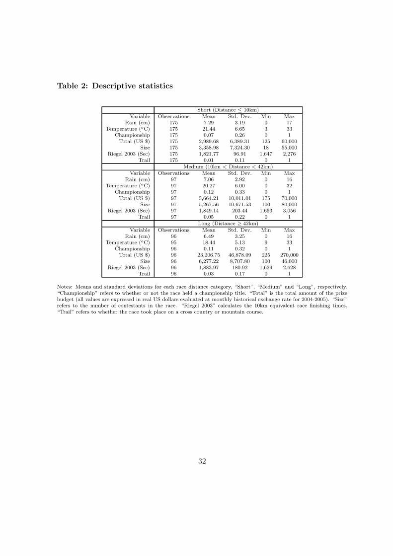
Table 2: Descriptive statistics

Short (Distance ≤ 10km)Variable Observations Mean Std. Dev. Min Max

Rain (cm) 175 7.29 3.19 0 17Temperature (oC) 175 21.44 6.65 3 33

Championship 175 0.07 0.26 0 1Total (US $) 175 2,989.68 6,389.31 125 60,000

Size 175 3,358.98 7,324.30 18 55,000Riegel 2003 (Sec) 175 1,821.77 96.91 1,647 2,276

Trail 175 0.01 0.11 0 1Medium (10km < Distance < 42km)

Variable Observations Mean Std. Dev. Min MaxRain (cm) 97 7.06 2.92 0 16

Temperature (oC) 97 20.27 6.00 0 32Championship 97 0.12 0.33 0 1

Total (US $) 97 5,664.21 10,011.01 175 70,000Size 97 5,267.56 10,671.53 100 80,000

Riegel 2003 (Sec) 97 1,849.14 203.44 1,653 3,056Trail 97 0.05 0.22 0 1

Long (Distance ≥ 42km)Variable Observations Mean Std. Dev. Min Max

Rain (cm) 96 6.49 3.25 0 16Temperature (oC) 95 18.44 5.13 9 33

Championship 96 0.11 0.32 0 1Total (US $) 96 23,206.75 46,878.09 225 270,000

Size 96 6,277.22 8,707.80 100 46,000Riegel 2003 (Sec) 96 1,883.97 180.92 1,629 2,628

Trail 96 0.03 0.17 0 1

Notes: Means and standard deviations for each race distance category, “Short”, “Medium” and “Long”, respectively.“Championship” refers to whether or not the race held a championship title. “Total” is the total amount of the prizebudget (all values are expressed in real US dollars evaluated at monthly historical exchange rate for 2004-2005). “Size”refers to the number of contestants in the race. “Riegel 2003” calculates the 10km equivalent race finishing times.“Trail” refers to whether the race took place on a cross country or mountain course.

32

Table 3: Prize structure without controls

PANEL AMeasures of Competitiveness

Dependent Variable C. I. 1:2 1:3 1:TotalDistance (km) 0.0008 0.0008 0.0007 0.0006

[0.0003]** [0.0002]** [0.0002]** [0.0004]Constant 0.394 0.6241 0.7321 0.4511

[0.0075]** [0.0058]** [0.0063]** [0.0102]**Observations 368 368 368 368

PANEL BMeasures of Competitiveness

Dependent Variable C. I. 1:2 1:3 1:TotalMedium 0.0119 0.0115 0.0112 0.0162

[0.0113] [0.0086] [0.0094] [0.0153]Long 0.0316 0.0299 0.025 0.0245

[0.0113]** [0.0087]** [0.0094]** [0.0153]Constant 0.3989 0.6292 0.7358 0.4531

[0.0067]** [0.0052]** [0.0056]** [0.0091]**Observations 368 368 368 368

Notes: Standard errors are in parentheses. (*) and (**) represent significance at the 95 and 99 percent level. Omittedgroup in Panel B is Short Distance.

33

Table 4: Prize structure with controls

PANEL AMeasures of Competitiveness

Dep. Var. C. I. C. I. 1:2 1:2 1:3 1:3 1:Total 1:TotalDist. 0.0008 0.0007 0.0008 0.0008 0.0007 0.0006 0.0006 0.0004

[0.0003]** [0.0003]* [0.0002]** [0.0003]** [0.0002]** [0.0003]* [0.0004] [0.0004]Rain -0.0059 -0.0037 -0.0037 -0.008

[0.0015]** [0.0011]** [0.0012]** [0.0019]**Temp. 0.0011 0.0007 0.0005 0.0005

[0.0007] [0.0006] [0.0006] [0.0010]Champ. 0.0006 -0.0034 -0.0039 -0.0206

[0.0156] [0.0121] [0.0131] [0.0203]Prize 0 0 0 0

[0.0000] [0.0000] [0.0000] [0.0000]†

Size 0 0 0 0[0.0000] [0.0000] [0.0000] [0.0000]

Riegel 0.0001 0 0.0001 0.0002[0.0000] [0.0000] [0.0000]† [0.0001]**

Trail -0.0148 -0.0067 -0.0398 -0.0991[0.0351] [0.0272] [0.0294] [0.0456]*

Const. 0.394 0.302 0.6241 0.6191 0.7321 0.6413 0.4511 0.0984[0.0075]** [0.0726]** [0.0058]** [0.0562]** [0.0063]** [0.0609]** [0.0102]** [0.0943]

Obs. 368 368 368 368 368 368 368 368

PANEL BMeasures of Competitiveness

Dep. Var. C. I. C. I. 1:2 1:2 1:3 1:3 1:Total 1:TotalMedium 0.0119 0.011 0.0115 0.0109 0.0112 0.0112 0.0162 0.0163

[0.0113] [0.0112] [0.0086] [0.0087] [0.0094] [0.0094] [0.0153] [0.0145]Long 0.0316 0.0291 0.0299 0.0289 0.025 0.0233 0.0245 0.0183

[0.0113]** [0.0122]* [0.0087]** [0.0094]** [0.0094]** [0.0102]* [0.0153] [0.0158]Rain -0.006 -0.0038 -0.0038 -0.0081

[0.0015]** [0.0011]** [0.0012]** [0.0019]**Temp. 0.0011 0.0007 0.0005 0.0006

[0.0007] [0.0006] [0.0006] [0.0010]Champ. 0 -0.0037 -0.0043 -0.0215

[0.0156] [0.0121] [0.0131] [0.0203]Prize 0 0 0 0

[0.0000] [0.0000] [0.0000] [0.0000]†

Size 0 0 0 0[0.0000] [0.0000] [0.0000] [0.0000]

Riegel 0.0001 0 0.0001 0.0002[0.0000]† [0.0000] [0.0000]* [0.0000]**

Trail -0.0163 -0.0092 -0.0424 -0.1021[0.0351] [0.0273] [0.0295] [0.0456]*

Const. 0.3989 0.3021 0.6292 0.6168 0.7358 0.6389 0.4531 0.096[0.0067]** [0.0726]** [0.0052]** [0.0564]** [0.0056]** [0.0610]** [0.0091]** [0.0944]

Obs. 368 368 368 368 368 368 368 368

Notes: Standard errors are in parentheses. (†), (*) and (**) represent significance at the 90, 95 and 99 percent level,respectively. For description of dependent variables see Table 2.

34

References

[1] Barut, Y., Kovenock, D. (1998) The Symmetric Multiple Prize All–Pay Auction

with Complete Information. European Journal of Political Economy 14(4), 627-

644.

[2] Baye, M., R., Kovenock, D., de Vries, C., G. (1996) The All–Pay Auction with

Complete Information. Economic Theory 8, 291-305.

[3] Burguet, R., Sakovics, J. (1999) Imperfect Competition in Auction Designs. In-

ternational Economic Review 40(1), 231-247.

[4] Clark, D., J., Riis, C. (1998a) Competition over more than one Prize. American

Economic Review 88, 276-289.

[5] Clark, D., J., Riis, C. (1998b) Influence and the Discretionary Allocation of Several

Prizes. European Journal of Political Economy 14, 605-625.

[6] Cohen, C., Sela, A. (2008) Allocation of Prizes in Asymmetric All–Pay Auctions.

European Journal of Political Economy, forthcoming.

[7] Ehrenberg, R., G, Bognanno, M., L. (1990a) Do Tounaments have Incentive Ef-

fects? Journal of Political Economy 98 (6), 1307-1324.

[8] Ehrenberg, R., G, Bognanno, M., L. (1990b) The Incentive Effects of Tournaments

Revisted: Evidence from the European PGA Tour. Industrial and Labor Relations

Review 43 (6), 74-88.

[9] Eriksson, T. (1999) Executive Compensation and Tournament Theory: Empirical

Tests on Danish Data. Journal of labor Economics 17 (2), 262-280.

[10] Frick, B. (2003) Contest Theory and Sport? Oxford Review of Economic Policy

19 (4), 512-529.

[11] Fullerton, R., L., McAfee, R., P. (1999) Auctioning Entry into Tournaments. Jour-

nal of Political Economy 107(3), 573-605.

35

[12] Glazer, A., Hassin, R. (1988) Optimal Contests. Economic Inquiry 26, 133-143.

[13] Green, J., Stokey, N. (1983) A Comparison of Tournaments and Contracts. Journal

of Political Economy 91, 349-364.

[14] Groh, C., Moldovanu, B., Sela, A., Sunde, U. (2008) Optimal Seedings in Elimi-

nation Tournaments. Economic Theory, forthcoming.

[15] Klemperer, P. (2002) How (not) to run auctions: The European 3G telecom auc-

tions. European Economic Review 46, 829-845.

[16] Krishna, V., Morgan, J. (1998) The Winner–Take–All Principle in Small Tourna-

ments. Advances in Applied Microeconomics 7, 61-74.

[17] Lazear, E., P. (1986) Salaries and Piece Rates. Journal of Business 59(3), 405-

431.

[18] Lazear, E., P., Rosen, S. (1981) Rank–Order Tournaments as Optimal Labor Con-

tracts. Journal of Political Economy 89(5), 841-864.

[19] Lynch, J., Zax, J., S. (2000) The Rewards to Running: Prize Structure and Perfor-

mance in Professional Road Racing. Journal of Sports Economics 1(4), 323-340.

[20] McAfee, R., P. (1993) Mechanism Design by Competing Sellers. Econometrica 61,

1281-1312.

[21] Maloney, M., T., McCormick, R., E. (2000) The Response of Workers to Wages

in Tornaments: Evidence from Foot Races. Journal of Sports Economics 1(2),

99-123.

[22] Moldovanu, B., Sela, A. (2001) The Optimal Allocation of Prizes in Contests.

American Economic Review 91(3), 542-558.

[23] Moldovanu, B., Sela, A. (2006) Contest Architecture. Journal of Economic Theory

126(1), 70-97.

36

[24] Moldovanu, B., Sela, A., Shi, X. (2007) Contests for Status. Journal of Political

Economy 115, 338-363.

[25] Moldovanu, B., Sela, A., Shi, X. (2008) Competing Auctions with Endogenous

Quantities. Journal of Economic Theory, forthcoming.

[26] Mookherjee, D. (1984) Optimal Incentive Schemes with Many Agents. Review of

Economic Studies 51, 433-446.

[27] Nalebuff, B., J., Stiglitz, J., E. (1983) Prizes and Incentives: Towards a General

Theory of Compensation and Competition. Bell Journal of Economics 14(1), 21-

43.

[28] Noakes, T., D. (1985) Lore of Running, Oxford: Oxford University Press.

[29] Nti, K., O. (1997) Comparative Statics of Contests and Rent–Seeking Games.

International Economic Review 38, 43-59.

[30] Perez–Castrillo, D., Verdier, T. (1992) A General Analysis of Rent–Seeking Games.

Public Choice 73, 335-350.

[31] Peters, M., Severinov, S. (1997) Competition among Sellers Who Offer Auctions

Instead of Prices. Journal of Economic Theory 75, 114-179.

[32] Rosen, S. (2001) Prizes and Incentives in Elimination Tournaments. American

Economic Review 76(4), 701-715.

[33] Skaderpas, S. (1996) Contest Success Functions. Economic Theory 7, 283-290.

[34] Szymanski, S., Valletti, T. (2005) Incentive Effects of Second Prizes. European

Journal of Political Economy 21, 467-481.

[35] Taleb, N., N. (2005) Fooled by Randomness: The Hidden Role of Chance in Life

and in the Markets, New York: Random House.

[36] Taylor, C., R. (1995) Digging for Goldon Carrots: An Analysis of Research Tour-

naments. American Economic Review 85(4), 872-890.

37

[37] Tullock, G. (1980) Efficient Rent Seeking. in: J. Buchanan et al. (Eds), Towards

a Theory of the Rent–Seeking Society, Texas A&M University Press, College Sta-

tion.

38