Compatible algorithms for coupled flow and transport q Clint Dawson * , Shuyu Sun, Mary F. Wheeler Center for Subsurface Modeling-C0200, Texas Institute for Computational Engineering and Sciences, The University of Texas at Austin, Austin, TX 78712, USA Received 10 April 2003; received in revised form 7 November 2003; accepted 18 December 2003 Abstract The issue of mass conservation in numerical methods for flow coupled to transport has been debated in the literature for the past several years. In this paper, we address the loss of accuracy and/or loss of global conservation which can occur when flow and transport schemes are not compatible. We give a definition of compatible flow and transport schemes, with emphasis on two popular types of transport algorithms, the streamline diffusion method and discon- tinuous Galerkin methods. We then discuss several different approaches for flow which are compatible with these transport algorithms. Finally, we give some numerical examples which demonstrate the possible effects of incompati- bility between schemes. Ó 2004 Elsevier B.V. All rights reserved. Keywords: Flow; Transport; Mass conservation; Streamline diffusion method; Discontinuous Galerkin methods 1. Introduction The transport of chemically reactive species arises in a number of important applications. Specific examples include groundwater contamination, water quality modeling and air quality modeling. This physical process is described by advection–diffusion–reaction systems. The advection and diffusion of chemical species are governed by a velocity field, which is generally given by a flow model. The flow model is application-dependent, and may be described, for example, by Darcy flow in the subsurface, a hydrodynamic model in shallow water or the Navier–Stokes equations. In each of these models, the velocity field satisfies a continuity equation (conservation of mass equation) of the form r u ¼ f ; ð1Þ where u is the velocity field, and f is an external source/sink function. q The first author was supported in part by NSF grant DMS-0107247. * Corresponding author. Tel.: +1-512-475-8627; fax: +1-512-471-8694. E-mail address: [email protected] (C. Dawson). 0045-7825/$ - see front matter Ó 2004 Elsevier B.V. All rights reserved. doi:10.1016/j.cma.2003.12.059 Comput. Methods Appl. Mech. Engrg. 193 (2004) 2565–2580 www.elsevier.com/locate/cma

Welcome message from author
This document is posted to help you gain knowledge. Please leave a comment to let me know what you think about it! Share it to your friends and learn new things together.
Transcript

Comput. Methods Appl. Mech. Engrg. 193 (2004) 2565–2580
www.elsevier.com/locate/cma
Compatible algorithms for coupled flow and transport q
Clint Dawson *, Shuyu Sun, Mary F. Wheeler
Center for Subsurface Modeling-C0200, Texas Institute for Computational Engineering and Sciences, The University of Texas at Austin,
Austin, TX 78712, USA
Received 10 April 2003; received in revised form 7 November 2003; accepted 18 December 2003
Abstract
The issue of mass conservation in numerical methods for flow coupled to transport has been debated in the literature
for the past several years. In this paper, we address the loss of accuracy and/or loss of global conservation which can
occur when flow and transport schemes are not compatible. We give a definition of compatible flow and transport
schemes, with emphasis on two popular types of transport algorithms, the streamline diffusion method and discon-
tinuous Galerkin methods. We then discuss several different approaches for flow which are compatible with these
transport algorithms. Finally, we give some numerical examples which demonstrate the possible effects of incompati-
bility between schemes.
� 2004 Elsevier B.V. All rights reserved.
Keywords: Flow; Transport; Mass conservation; Streamline diffusion method; Discontinuous Galerkin methods
1. Introduction
The transport of chemically reactive species arises in a number of important applications. Specific
examples include groundwater contamination, water quality modeling and air quality modeling. This
physical process is described by advection–diffusion–reaction systems.The advection and diffusion of chemical species are governed by a velocity field, which is generally given
by a flow model. The flow model is application-dependent, and may be described, for example, by Darcy
flow in the subsurface, a hydrodynamic model in shallow water or the Navier–Stokes equations. In each of
these models, the velocity field satisfies a continuity equation (conservation of mass equation) of the form
r � u ¼ f ; ð1Þwhere u is the velocity field, and f is an external source/sink function.
qThe first author was supported in part by NSF grant DMS-0107247.* Corresponding author. Tel.: +1-512-475-8627; fax: +1-512-471-8694.
E-mail address: [email protected] (C. Dawson).
0045-7825/$ - see front matter � 2004 Elsevier B.V. All rights reserved.
doi:10.1016/j.cma.2003.12.059

2566 C. Dawson et al. / Comput. Methods Appl. Mech. Engrg. 193 (2004) 2565–2580
We will consider transport equations for each chemical species of the form
oð/ciÞot
þr � ðuci � DðuÞrciÞ ¼ f~ci þ Riðc1; . . . ; cnÞ; ð2Þ
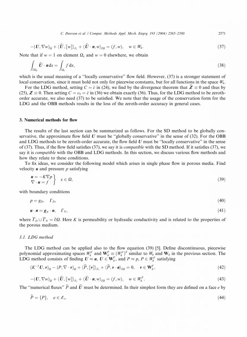
where ci denotes the concentration of species i, i ¼ 1; . . . ; nc; nc is the number of chemical species, DðuÞ is a(possibly) velocity-dependent diffusion/dispersion tensor which is symmetric and positive semi-definite, / is
a volumetric factor such as porosity, and Ri is a chemical reaction term. The concentration ~ci is usually
specified at sources (where f > 0) and ~ci ¼ ci at sinks ðf < 0Þ. In some cases, there could be feedback fromthe transport model to the flow model; that is, u ¼ uðc1; . . . ; cncÞ.
It is well known that in many cases (2) is advection-dominated, which can lead to steep concentration
gradients. Moreover, these concentration fronts may be made even steeper by the presence of chemical
reactions. Therefore, when solving (2) numerically, it is essential that the numerical method preserve these
steep gradients with minimal oscillation and numerical diffusion. The transport method should also be
provably accurate, at least for smooth solutions, and satisfy global conservation of chemical mass.
In recent years, there has been discussion in the literature about ‘‘locally conservative’’ methods for flow
and transport; see, for example [3,6,10,15]. Local conservation refers to conservation of mass or species overa control volume or an element in a finite element or finite difference grid. Local conservation combined with
flux continuity guarantees global conservation of a numerical scheme. For a number of transport schemes,
local conservation is a by-product of the fact that these schemes use discontinuous approximating spaces
combined with numerical fluxes to model advection-dominated transport. When modeling flow on its own,
local conservation, in the sense of satisfying (1) locally, may or may not be important. However, when
coupling flow with transport, how the flow model handles (1) can be quite important, and can directly affect
the accuracy and conservation properties of the transport method.
In this paper, we address the numerical modeling of coupled flow and transport. Our goal is to determine‘‘compatible’’ numerical methods for flow and transport. That is, we wish to determine the minimal
requirements on the flow algorithm to maintain certain accuracy and conservation properties of the
numerical method used for transport. In order to fix ideas, we will consider three transport algorithms: the
Streamline Diffusion (SD) method [4,12,13], and two variants of the discontinuous Galerkin (DG) method,
the local discontinuous Galerkin method (LDG) [7–9] and the primal discontinuous Galerkin methods
[14,16,22]. The SD method uses a standard, continuous Galerkin formulation. Both DG methods use
discontinuous approximating spaces defined over each element. These methods are all globally conserva-
tive, stable and accurate given the true velocity field u. However, they may lose these properties, dependingon how one approximates u. In particular, our primary result in this paper is that appropriately satisfying
(1) numerically is crucial to preserving the accuracy, stability and global conservation properties of these
transport methods.
The paper is organized as follows. In the next section, we briefly describe the SD and DG transport
algorithms and discuss their accuracy and conservation properties. In Section 3, we discuss several flow
algorithms for the specific case of an elliptic, stationary flow problem, with emphasis on how these algorithms
approximate (1). These include the standard continuous Galerkin method, the mixed finite element method,
and DG methods based on the primal and dual forms of the flow equation. In particular, we discuss thecompatibility of these algorithms with the SD and DG transport schemes. Finally, in Section 4, we give some
numerical results which further illuminate our findings, followed by conclusions and further discussion.
2. The streamline diffusion and discontinuous Galerkin transport algorithms
In order to simplify the discussion, we consider the following single transport equation:
ct þr � ðuc� DrcÞ ¼ f~c; ðx; tÞ 2 X� ð0; T �; ð3Þ

C. Dawson et al. / Comput. Methods Appl. Mech. Engrg. 193 (2004) 2565–2580 2567
defined on an open, fixed domain X 2 Rd with smooth boundary oX. Let n denote the unit outward normal
to oX. We assume oX is divided into inflow and noflow/outflow regions
CI ¼ fx 2 oX : u � n < 0g; ð4Þ
CO ¼ fx 2 oX : u � nP 0g: ð5Þ
On these boundaries we assume the boundary conditions,
ðcu� DrcÞ � n ¼ cIu � n; CI � ð0; T �; ð6Þ
ðDrcÞ � n ¼ 0; CO � ð0; T �: ð7Þ
We also impose the initial condition
cðx; 0Þ ¼ c0ðxÞ; x 2 X: ð8ÞWe discretize X by a finite element partition Th of elements Xe with diameter he. Let h denote the
maximal element diameter. Let Dt > 0 denote a time step, with tn ¼ nDt, n ¼ 0; 1; . . . Denote by Sn the
space–time slab X� ½tn; tnþ1Þ. We discretize Sn by a space–time finite element partition TnDt;h. Assuming
Dt ¼ OðhÞ, the maximal element diameter in TnDt;h is also OðhÞ.
We denote by ð�; �ÞR the standard L2 inner product over domain R. Surface integrals are denoted by h�; �iR.
2.1. The SD method
The SD method is based on the following reformulation of (3). Using (1), we write
r � ðucÞ ¼ u � rcþ fc ð9Þ
and
ct þ u � rc�r � ðDrcÞ ¼ f ð~c� cÞ; ðx; tÞ 2 X� ð0; T �: ð10ÞLet V n
h denote the space of continuous, piecewise linear functions in space and piecewise linears in time
defined on the partition TnDt;h of the slab Sn. Note that these functions may be discontinuous from one slab
to the next. Therefore, we denote by
v�ðtnÞ ¼ lims!0�
vðx; tn þ sÞ: ð11Þ
The SD diffusion method then is to find C 2 V nh satisfying, for n ¼ 0
ðC�ð�; 0Þ � c0ð�Þ; vþð�; 0ÞÞX ¼ 0; v 2 V 0h ð12Þ
and for each n ¼ 0; 1; . . .,
ðCt þ u � rC; vþ dðvt þ u � rvÞÞSn þ ðDrC;rvÞSn þ hu � nðcI � CÞ; viCI�ðtn;tnþ1Þ
þ ðCþð�; tnÞ � C�ð�; tnÞ; vþð�; tnÞÞX ¼ ðf ðeC � CÞ; vÞSn ; v 2 V nh : ð13Þ
The parameter d is typically chosen to be OðhÞ, but can also be chosen depending on the size of D [12].
2.2. The OBB method
The Oden–Babu�ska–Baumann discontinuous Galerkin method uses completely discontinuous approx-
imating spaces to approximate c. Let

2568 C. Dawson et al. / Comput. Methods Appl. Mech. Engrg. 193 (2004) 2565–2580
Wh ¼ fw : wjXe2 PkðXeÞg;
where Pk denotes the space of complete polynomials of degree kP 1. We also need some additionalnotation. For adjacent elements Xþ
e and X�e with unit outward normals n�, let w� denote the trace of w on
the face e between X�e from the interiors of the elements. Define the average f�g and jump s � t for x 2 e as
follows:
fwg ¼ ðw� þ wþÞ=2; ð14Þ
swt ¼ wþnþ þ w�n�: ð15ÞFurthermore, for x 2 e, define the upwind value of w as follows:
wu ¼ w�; u � n� > 0;wþ; u � nþ > 0:
�ð16Þ
Let Ei denote the set of all interior element faces in the finite element mesh.
The OBB method (in continuous time) is then defined as follows. Find Cð�; tÞ 2 Wh satisfying
ðCð�; 0Þ � c0;wÞX ¼ 0; w 2 Wh ð17Þand for t > 0
ðCt;wÞX � ðuC � DrC;rwÞX þ hCuu� fDrCg; swtiEiþ hfDrwg; sCtiEi
þ hcIu � n;wiCI
þ hCu � n;wiCO¼ ðf eC ;wÞX; w 2 Wh: ð18Þ
2.3. The LDG method
The local discontinuous Galerkin method also uses completely discontinuous approximating spaces. The
method defines two auxiliary variables
~z ¼ �rc; ð19Þ
z ¼ D~z ð20Þand approximates z and ~z by functions Z and eZ in the space
Wh ¼ ðWhÞd : ð21ÞFor functions v 2 Wh we define
svt ¼ v � nþ þ v � n�
analogous to (15). The scheme differs from the OBB method in the way that the diffusion term is handled.Advection is handled in exactly the same way as in the OBB method.
The LDG method is defined as follows. Find Cð�; tÞ 2 Wh, Z, eZ 2 Wh, satisfying
ðCð�; 0Þ � c0;wÞX ¼ 0; w 2 Wh ð22Þand for t > 0
ðCt;wÞX � ðuC þ Z;rwÞX þ hCuuþ Z�; swtiEiþ hcIu � n;wiCI
þ hCu � n;wiCO¼ ðf eC ;wÞX; w 2 Wh;
ð23Þ
ð eZ ; vÞX � ðC;r � vÞX þ hCþ; svtiEiþ hC; v � nioX ¼ 0; v 2 Wh; ð24Þ

C. Dawson et al. / Comput. Methods Appl. Mech. Engrg. 193 (2004) 2565–2580 2569
ðZ;~vÞX ¼ ðD eZ ;~vÞX; ~v 2 Wh: ð25ÞWe note that, because eZ and v are discontinuous, eZ can be eliminated element by element in terms of C in
(24). Similarly, Z can be eliminated element by element in terms of eZ by (25). Substituting into (23), we
obtain a system in C only.
2.4. Accuracy and global conservation
The schemes outlined above have all been proven to be stable, and through a priori error analysis, to beaccurate for smooth solutions c [8,12,16]. In particular, they all satisfy error estimates of the form
max06 t6 T
kc� CkL2ðXÞ 6Khp; ð26Þ
for some exponent pP 1 depending on the polynomial degree, and K a constant independent of h. Thisanalysis assumes the true velocity u is known. An analysis of the DG method with approximate velocity Ucan be found in [10].
Furthermore, each method is globally conservative in the following sense. Integrating (3) over X� ð0; tkÞand applying the boundary and initial conditions, we findZ
Xcðx; tkÞdxþ
Z tk
0
ZCO
cu � ndsdt ¼ZXc0ðxÞdx�
Z tk
0
ZCI
cIu � ndsdt þZ tk
0
ZXf~cdxdt: ð27Þ
For the SD method for example, setting v � 1 on Sn, n ¼ 1; . . . ; k and using the fact that r � u ¼ f , we findfrom (13),
ZXC�ðx; tkÞdxþ
Z tk
0
ZCO
Cu � ndsdt ¼ZXc0ðxÞdx�
Z tk
0
ZCI
cIu � ndsdt þZ tk
0
ZXf eC dxdt: ð28Þ
Similar statements hold for the OBB and LDG methods.Now we ask, what happens to the accuracy and global mass conservation properties of these methods if
u � U . In particular, we ask
1. Is the scheme still zeroth-order accurate; that is, if the solution c is identically a constant, do the methods
reproduce c?2. Is the scheme still globally conservative in the sense of (28) (with U replacing u)?
With respect to question 1, we note that if the initial, boundary and source data are all equal to aconstant c, then c � c for all time. The ability to reproduce a constant may seem trivial, but it is important
in many transport applications. In particular, it is often the case that the solution c is constant over large
parts of the domain for long periods of time. If the transport scheme can no longer reproduce a constant
when U � u, then spurious sources and sinks can be created in the transport solution, which can lead to
numerical inaccuracy (overshoot and undershoot) of the solution.
We now address questions 1 and 2 above with respect to each of the transport schemes.
First, we note that when using a numerical method to compute u, it is possible that the computed
velocity may not have a uniquely defined normal component across each element face, particularly if U isdiscontinuous. However, all of our transport schemes rely on knowing U � n on certain element faces. We
will assume in the discussion below that such a quantity is known on each edge, either as part of the flow
computation or by postprocessing U , and to be consistent with our discussion in Section 3, we denote this
quantity as bU � n.

2570 C. Dawson et al. / Comput. Methods Appl. Mech. Engrg. 193 (2004) 2565–2580
2.5. SD method with approximate u
We consider now (13) with U replacing u; that is
ðCt þU � rC; vþ dðvt þU � rvÞÞSn þ ðDrC;rvÞSn þ h bU � nðcI � CÞ; viCI�ðtn;tnþ1Þ
þ ðCþð�; tnÞ � C�ð�; tnÞ; vþð�; tnÞÞX ¼ ðf ðeC � CÞ; vÞSn ; v 2 V nh : ð29Þ
It is easily seen that if c0 ¼ cI ¼ eC ¼ c, then C � c satisfies (29) independent of U . Thus, since C is unique,
the SD method is always zeroth-order accurate.
To check for global conservation, set v � 1 in (29), then
ðCt þU � rC; 1ÞSn þ h bU � nðcI � CÞ; 1iCI�ðtn;tnþ1Þ þ ðCþð�; tnÞ � C�ð�; tnÞ; 1ÞX ¼ ðf ðeC � CÞ; 1ÞSn : ð30Þ
Summing on n and using (12) we find
ðC�ðx; tkÞ; 1ÞX þXk�1
n¼0
½ðU ;rCÞSn þ h bU � n; cI � CiCI�ðtn;tnþ1Þ� ¼ ðc0; 1ÞX þXk�1
n¼0
ðf ; eC � CÞSn : ð31Þ
In order to obtain the analogue of (28), U and bU should satisfy
�ðU ;rvÞSn þ h bU � n; vioX�ðtn;tnþ1Þ ¼ ðf ; vÞSn ; v 2 V nh : ð32Þ
That is, setting v ¼ C in (32) and substituting into (31) gives (28) with u replaced by U . Setting v � 1, we
obtainZ tnþ1
tn
ZoX
bU � ndsdt ¼Z tnþ1
tn
ZXf dxdt; ð33Þ
which is a statement of ‘‘global conservation’’ of the flow field U; (32) is a more stringent requirement.
2.6. The OBB and LDG methods with approximate u
The OBB method with U replacing u is given by
ðCt;wÞX � ðUC � DrC;rwÞX þ hCu bU � fDrCg; swtiEiþ hfDrwgsCtiEi
þ hcI bU � n;wiCI
þ hC bU � n;wiCO¼ ðf eC ;wÞX; w 2 Wh: ð34Þ
Setting w � 1 and integrating in time, we findZXCðx; tkÞdxþ
Z tk
0
ZCO
C bU � ndsdt ¼ZXc0ðxÞdx�
Z tk
0
ZCI
cI bU � ndsdt þZ tk
0
ZXf eC dxdt: ð35Þ
Similarly, setting w � 1 in (23), we obtain the same result. Thus, both the OBB and LDG methods are
globally conservative, in the sense of (35), independent of how U is computed.Now we check to see whether these schemes are zeroth-order accurate. First, we check to see whether or
not C ¼ cI ¼ c satisfies (34). The left side of (34) becomes
ch�ðU ;rwÞX þ h bU ; swtiEi
þ h bU � n;wioXi: ð36Þ
For this term to be equal to
cðf ;wÞX;which is the right-hand side of (34) in this case, we need (for c 6¼ 0)
C. Dawson et al. / Comput. Methods Appl. Mech. Engrg. 193 (2004) 2565–2580 2571
�ðU ;rwÞX þ h bU ; swtiEiþ h bU � n;wioX ¼ ðf ;wÞ; w 2 Wh: ð37Þ
Note that if w ¼ 1 on element Xe and w ¼ 0 elsewhere, we obtainZoXe
bU � nds ¼ZXe
f dx; ð38Þ
which is the usual meaning of a ‘‘locally conservative’’ flow field. However, (37) is a stronger statement of
local conservation, since it must hold not only for piecewise constants, but for all functions in the space Wh.
For the LDG method, setting C ¼ c in (24), we find by the divergence theorem that eZ � 0 and thus by
(25), Z � 0. Then setting C ¼ cI ¼ c in (36) we obtain exactly (36). Thus, for the LDG method to be zeroth-
order accurate, we also need (37) to be satisfied. We note that the usage of the conservation form for the
LDG and the OBB methods results in the loss of the zeroth-order accuracy in general cases.
3. Numerical methods for flow
The results of the last section can be summarized as follows. For the SD method to be globally con-
servative, the approximate flow field U must be ‘‘globally conservative’’ in the sense of (32). For the OBB
and LDG methods to be zeroth-order accurate, the flow field U must be ‘‘locally conservative’’ in the sense
of (37). Thus, if the flow field satisfies (37), we say it is compatible with the SD method. If it satisfies (37), we
say it is compatible with the OBB and LDG methods. In this section, we discuss various flow methods and
how they relate to these conditions.To fix ideas, we consider the following model which arises in single phase flow in porous media. Find
velocity u and pressure p satisfying
u ¼ �Krpr � u ¼ f
�x 2 X; ð39Þ
with boundary conditions
p ¼ gD; CD; ð40Þ
u � n ¼ gN � n; CN ; ð41Þ
where CD [ CN ¼ oX. Here K is permeability or hydraulic conductivity and is related to the properties of
the porous medium.
3.1. LDG method
The LDG method can be applied also to the flow equation (39) [5]. Define discontinuous, piecewisepolynomial approximating spaces W F
h and WFh � ðW F
h Þd similar to Wh and Wh in the previous section. The
LDG method consists of finding U � u, U 2 WFh , and P � p, P 2 W F
h satisfying
ðK�1U ; vÞX � ðP ;r � vÞX þ hbP ; svtiEiþ hbP ; v � nioX ¼ 0; v 2 WF
h ; ð42Þ
�ðU ;rwÞX þ h bU ; swtiEiþ h bU � n;wioX ¼ ðf ;wÞ; w 2 W F
h : ð43Þ
The ‘‘numerical fluxes’’ bP and bU must be determined. In their simplest form they are defined on a face e by
bP ¼ fPg; e 2 Ei; ð44Þ
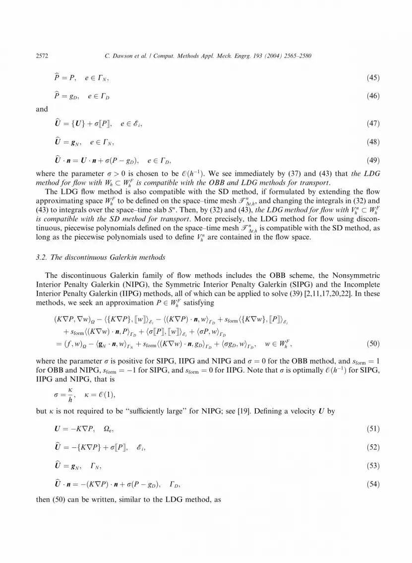
2572 C. Dawson et al. / Comput. Methods Appl. Mech. Engrg. 193 (2004) 2565–2580
bP ¼ P ; e 2 CN ; ð45Þ
bP ¼ gD; e 2 CD ð46Þand
bU ¼ fUg þ rsPt; e 2 Ei; ð47Þ
bU ¼ gN ; e 2 CN ; ð48Þ
bU � n ¼ U � nþ rðP � gDÞ; e 2 CD; ð49Þwhere the parameter r > 0 is chosen to be Oðh�1Þ. We see immediately by (37) and (43) that the LDG
method for flow with Wh � W Fh is compatible with the OBB and LDG methods for transport.
The LDG flow method is also compatible with the SD method, if formulated by extending the flow
approximating space W Fh to be defined on the space–time mesh Tn
Dt;h, and changing the integrals in (32) and
(43) to integrals over the space–time slab Sn. Then, by (32) and (43), the LDG method for flow with V nh � W F
h
is compatible with the SD method for transport. More precisely, the LDG method for flow using discon-
tinuous, piecewise polynomials defined on the space–time mesh TnDt;h is compatible with the SD method, as
long as the piecewise polynomials used to define V nh are contained in the flow space.
3.2. The discontinuous Galerkin methods
The discontinuous Galerkin family of flow methods includes the OBB scheme, the Nonsymmetric
Interior Penalty Galerkin (NIPG), the Symmetric Interior Penalty Galerkin (SIPG) and the Incomplete
Interior Penalty Galerkin (IIPG) methods, all of which can be applied to solve (39) [2,11,17,20,22]. In these
methods, we seek an approximation P 2 W Fh satisfying
ðKrP ;rwÞX � hfKrPg; swtiEi� hðKrP Þ � n;wiCD
þ sformhfKrwg; sPtiEi
þ sformhðKrwÞ � n; P iCDþ hrsPt; swtiEi
þ hrP ;wiCD
¼ ðf ;wÞX � hgN � n;wiCNþ sformhðKrwÞ � n; gDiCD
þ hrgD;wiCD; w 2 W F
h ; ð50Þ
where the parameter r is positive for SIPG, IIPG and NIPG and r ¼ 0 for the OBB method, and sform ¼ 1
for OBB and NIPG, sform ¼ �1 for SIPG, and sform ¼ 0 for IIPG. Note that r is optimally Oðh�1Þ for SIPG,
IIPG and NIPG, that is
r ¼ jh; j ¼ Oð1Þ;
but j is not required to be ‘‘sufficiently large’’ for NIPG; see [19]. Defining a velocity U by
U ¼ �KrP ; Xe; ð51Þ
bU ¼ �fKrPg þ rsPt; Ei; ð52Þ
bU ¼ gN ; CN ; ð53Þ
bU � n ¼ �ðKrPÞ � nþ rðP � gDÞ; CD; ð54Þ
then (50) can be written, similar to the LDG method, as
C. Dawson et al. / Comput. Methods Appl. Mech. Engrg. 193 (2004) 2565–2580 2573
�ðU ;rwÞX þ h bU ; swtiEiþ h bU � n;wioX þ sformhfKrwg; sPtiEi
¼ ðf ;wÞ þ sformhðKrwÞ � n; gD � P iCD; w 2 W F
h : ð55Þ
Thus, the OBB, NIPG and SIPG methods do not quite satisfy (37) or (32). However, the IIPG method for
flow with Wh � W Fh is compatible with the OBB and LDG methods for transport. Moreover, the IIPG method
for flow using discontinuous, piecewise polynomials defined on the space–time mesh TnDt;h is compatible with
the SD method, as long as the piecewise polynomials used to define V nh are contained in the flow space.
3.3. The standard Galerkin method
Another approach for flow which can be made compatible with the SD method is to use a standardGalerkin finite element method to compute an approximation to p. Here, we would seek P 2 V n
h \ fv : v ¼gD on CDg satisfying
ðKrP ;rvÞSn þ hgN � n; viCN�ðtn;tnþ1Þ ¼ ðf ; vÞSn ð56Þ
for all v 2 V nh with v ¼ 0 on CD. Defining U ¼ �KrP on Sn and bU ¼ gN on CN , we have
�ðU ;rvÞSn þ h bU � n; viCN�ðtn;tnþ1Þ ¼ ðf ; vÞSn : ð57Þ
Thus, we almost have (32) except that we do not have a flux defined on CD. We can however, postprocess
and obtain a flux on CD.
Let V nh;D be the set of functions in V n
h which are nonzero on CD. Then, find a 2 V nh;D satisfying
ha; viCD�ðtn;tnþ1Þ ¼ ðf ; vÞSn þ ðU ;rvÞSn � h bU � n; viCN�ðtn;tnþ1Þ; v 2 V nh;D: ð58Þ
Define the flux bU � n ¼ a on CD � ðtn; tnþ1Þ. Combining (57) and (58) we obtain (32).
3.4. The mixed finite element method
Finally, we briefly mention another popular method for solving (39), the mixed finite element method(MFE) [18]. The MFE method solves for approximations to both u and p simultaneously, similar to the
LDG method. However, in the MFE method the velocity space WFh � Hðdiv;XÞ; thus, functions in this
space have continuous normal component across element faces. The pressure space Wh satisfies
r �WFh ¼ Wh, and generally consists of discontinuous, piecewise polynomials. Define
WFh;g ¼ WF
h \ fv : v � n ¼ g � n on CNg:
Then, in the MFE, we seek U 2 WFh;gN
and P 2 W Fh satisfying
ðK�1U ; vÞX � ðP ;r � vÞX ¼ hgD; v � niCD; v 2 WF
h;0; ð59Þ
ðr �U ;wÞX ¼ ðf ;wÞX; w 2 W Fh : ð60Þ
By the continuity of the normal flux U � n, one can integrate (60) by parts to obtain
�ðU ;rwÞX þ hU � n; swtiEiþ hU � n;wiCD
¼ ðf ;wÞX � hgN � n;wiCN: ð61Þ
Thus, the MFE method is compatible with the OBB and LDG transport methods if Wh 2 W Fh , and it is
compatible with the SD method if mixed finite element spaces can be constructed on the partition TnDt;h
such that V nh � W F
h .
2574 C. Dawson et al. / Comput. Methods Appl. Mech. Engrg. 193 (2004) 2565–2580
4. Numerical results
In this section, we present some numerical results examining the compatibility of the various flow and
transport schemes outlined above.
We first consider the one-dimensional transport equation
ct þ ðucÞx � Dcxx ¼ fc; 0 < x < 1; t > 0 ð62Þwith u ¼ cosðpx=2Þ and f ¼ ux ¼ �p=2 sinðpx=2Þ. D is chosen to be 0.001. We choose K ¼ 1 in (39) with
Dirichlet boundary conditions pð0Þ ¼ 0 and pð1Þ ¼ �2=p. The flow direction then is from left to right, and
we specify inflow concentration cI at x ¼ 0. We consider the LDG and SD methods for transport, coupled
to the LDG and standard Galerkin methods for flow.
In the LDG method, we take piecewise linear approximations for both flow and transport. Thus, (37) is
satisfied. In computing flow, the penalty r ¼ 1=h. For (62), we integrate in time using a second order,
explicit Runge–Kutta method and apply a slope limiter at each step in the computation [1].For the standard Galerkin method for flow, the velocity bU has been computed on interior faces using a
postprocessing method described in [3], which gives a locally conservative flux in one space dimension in the
sense of (38). However, this postprocessed flow field is still not compatible with the LDG transport scheme
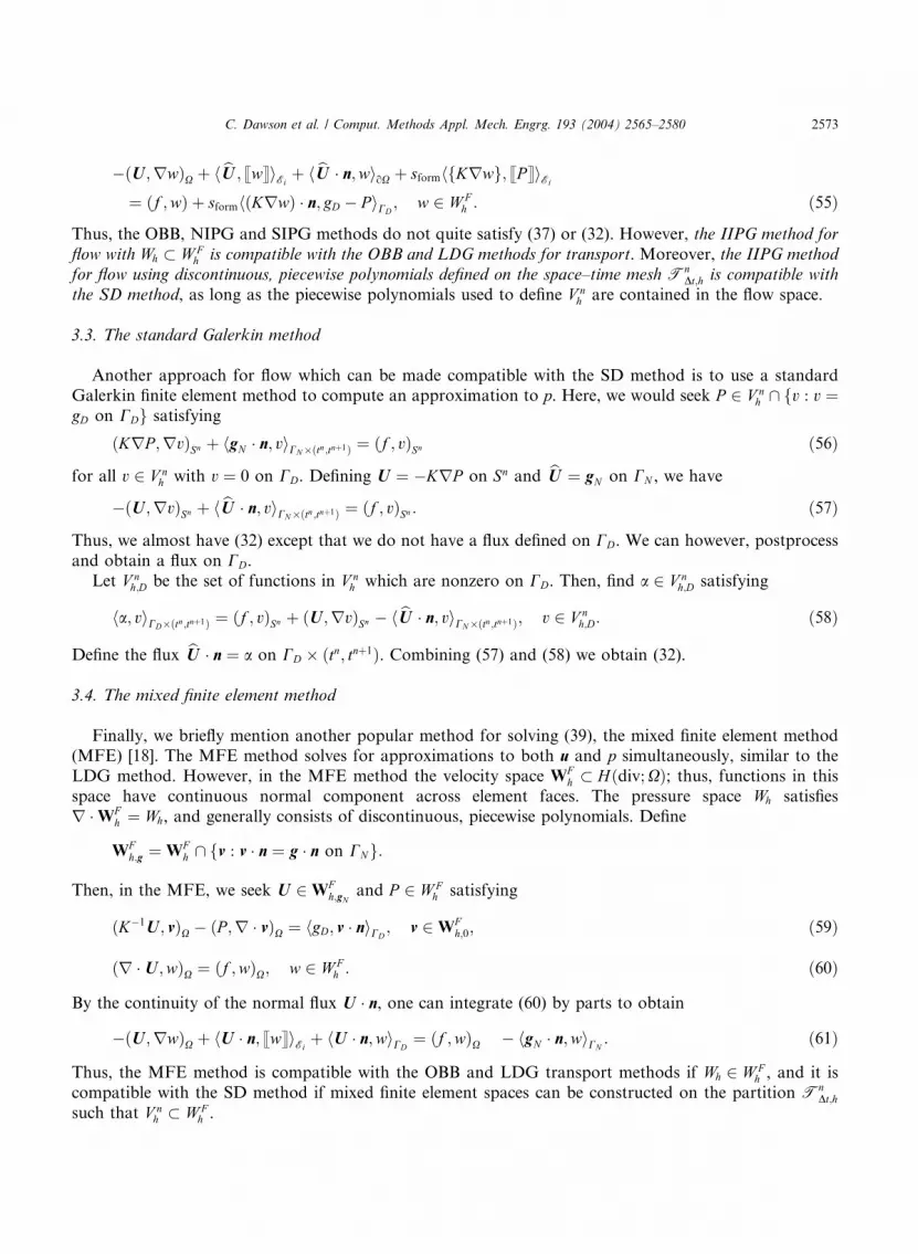
using piecewise linears, because it only satisfies (37) for piecewise constant functions w.In our first experiment, we test the LDG method for a constant solution of c � 1, obtained by setting the
inflow concentration cI and initial condition c0 both equal to one. We discretize the interval ½0; 1� with 50
grids blocks, solve the flow equation with f , K, pð0Þ and pð1Þ as described above, and then run a transport
simulation up to time T ¼ 0:5. Here we are testing the ability of the LDG method to propagate a constantexactly for many time steps. As seen in Fig. 1, when using LDG for flow we obtain the constant solution
c � 1. When using standard Galerkin for flow, we seem some overshoot and undershoot of the profile. This
exhibits the fact that flow fields which do not satisfy the compatibility condition (37) can introduce spurious
sources and sinks into the LDG transport solution.
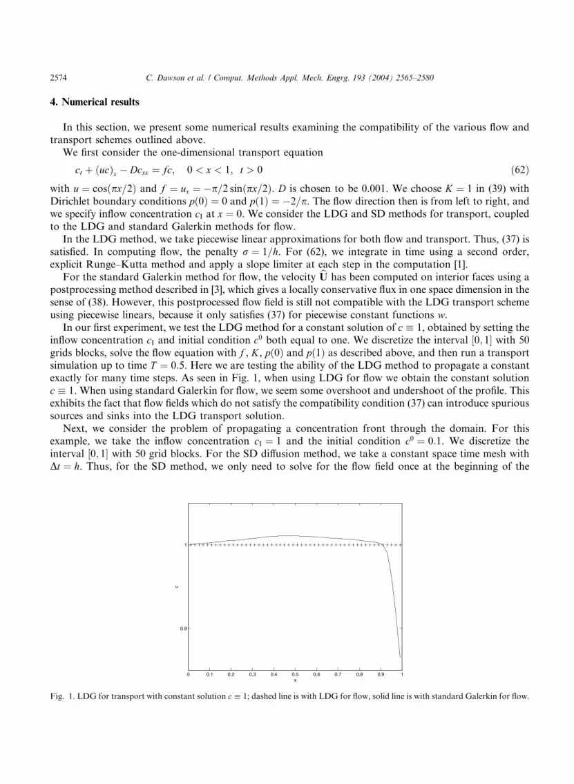
Next, we consider the problem of propagating a concentration front through the domain. For this
example, we take the inflow concentration cI ¼ 1 and the initial condition c0 ¼ 0:1. We discretize the
interval ½0; 1� with 50 grid blocks. For the SD diffusion method, we take a constant space time mesh with
Dt ¼ h. Thus, for the SD method, we only need to solve for the flow field once at the beginning of the
0 0.1 0.2 0.3 0.4 0.5 0.6 0.7 0.8 0.9 1
0.9
1
x
c
Fig. 1. LDG for transport with constant solution c � 1; dashed line is with LDG for flow, solid line is with standard Galerkin for flow.
C. Dawson et al. / Comput. Methods Appl. Mech. Engrg. 193 (2004) 2565–2580 2575
simulation. We have also implemented a shock-capturing algorithm described in [12], whereby we replace Din (62) by bD ¼ maxðD; c2h2jct þ ucxjÞ and d ¼ c1 maxð0;Dt � bDÞ. The parameters c1 and c2 were chosen to
be 0.1. The solutions obtained by the SD method at T ¼ 0:5 with the LDG and standard Galerkin flow
methods are given in Fig. 2. Note that both flow methods give virtually identical transport solutions,
namely a traveling front joining two constant regions where c ¼ 1 and c ¼ 0:1. Moreover, they are both
compatible with the SD method, and the mass conservation errors are within computer roundoff.
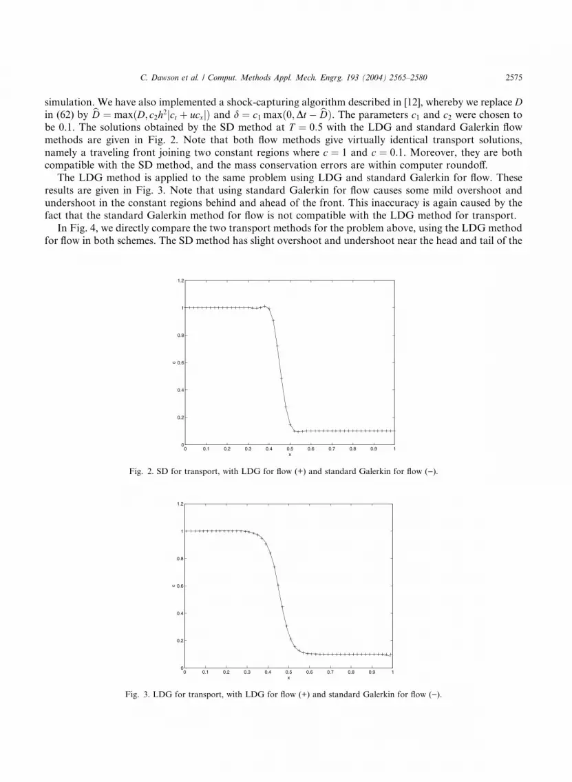
The LDG method is applied to the same problem using LDG and standard Galerkin for flow. These
results are given in Fig. 3. Note that using standard Galerkin for flow causes some mild overshoot and
undershoot in the constant regions behind and ahead of the front. This inaccuracy is again caused by thefact that the standard Galerkin method for flow is not compatible with the LDG method for transport.
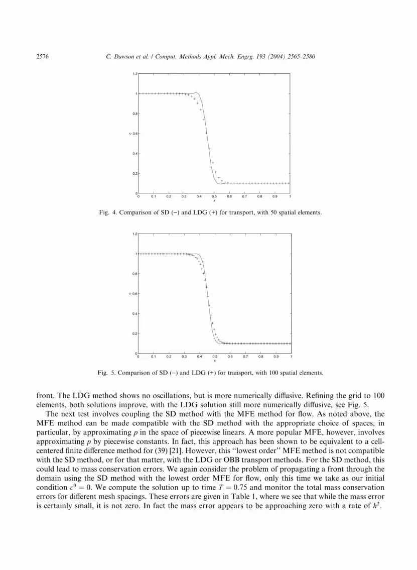
In Fig. 4, we directly compare the two transport methods for the problem above, using the LDG method
for flow in both schemes. The SD method has slight overshoot and undershoot near the head and tail of the
0 0.1 0.2 0.3 0.4 0.5 0.6 0.7 0.8 0.9 10
0.2
0.4
0.6
0.8
1
1.2
x
c
Fig. 3. LDG for transport, with LDG for flow (+) and standard Galerkin for flow ()).
0 0.1 0.2 0.3 0.4 0.5 0.6 0.7 0.8 0.9 10
0.2
0.4
0.6
0.8
1
1.2
x
c
Fig. 2. SD for transport, with LDG for flow (+) and standard Galerkin for flow ()).
0 0.1 0.2 0.3 0.4 0.5 0.6 0.7 0.8 0.9 10
0.2
0.4
0.6
0.8
1
1.2
x
c
Fig. 4. Comparison of SD ()) and LDG (+) for transport, with 50 spatial elements.
0 0.1 0.2 0.3 0.4 0.5 0.6 0.7 0.8 0.9 10
0.2
0.4
0.6
0.8
1
1.2
x
c
Fig. 5. Comparison of SD ()) and LDG (+) for transport, with 100 spatial elements.
2576 C. Dawson et al. / Comput. Methods Appl. Mech. Engrg. 193 (2004) 2565–2580
front. The LDG method shows no oscillations, but is more numerically diffusive. Refining the grid to 100elements, both solutions improve, with the LDG solution still more numerically diffusive, see Fig. 5.
The next test involves coupling the SD method with the MFE method for flow. As noted above, the
MFE method can be made compatible with the SD method with the appropriate choice of spaces, in
particular, by approximating p in the space of piecewise linears. A more popular MFE, however, involves
approximating p by piecewise constants. In fact, this approach has been shown to be equivalent to a cell-
centered finite difference method for (39) [21]. However, this ‘‘lowest order’’ MFE method is not compatible
with the SD method, or for that matter, with the LDG or OBB transport methods. For the SD method, this
could lead to mass conservation errors. We again consider the problem of propagating a front through thedomain using the SD method with the lowest order MFE for flow, only this time we take as our initial
condition c0 ¼ 0. We compute the solution up to time T ¼ 0:75 and monitor the total mass conservation
errors for different mesh spacings. These errors are given in Table 1, where we see that while the mass error
is certainly small, it is not zero. In fact the mass error appears to be approaching zero with a rate of h2.
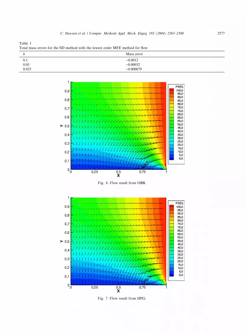
Table 1
Total mass errors for the SD method with the lowest order MFE method for flow
h Mass error
0.1 )0.00120.05 )0.000320.025 )0.000079
Fig. 6. Flow result from OBB.
Fig. 7. Flow result from IIPG.
C. Dawson et al. / Comput. Methods Appl. Mech. Engrg. 193 (2004) 2565–2580 2577
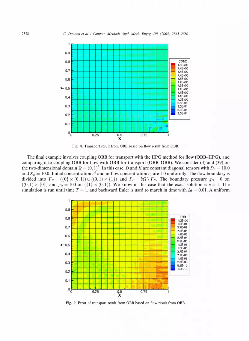
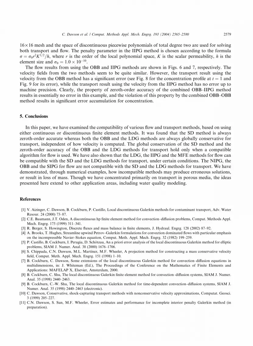
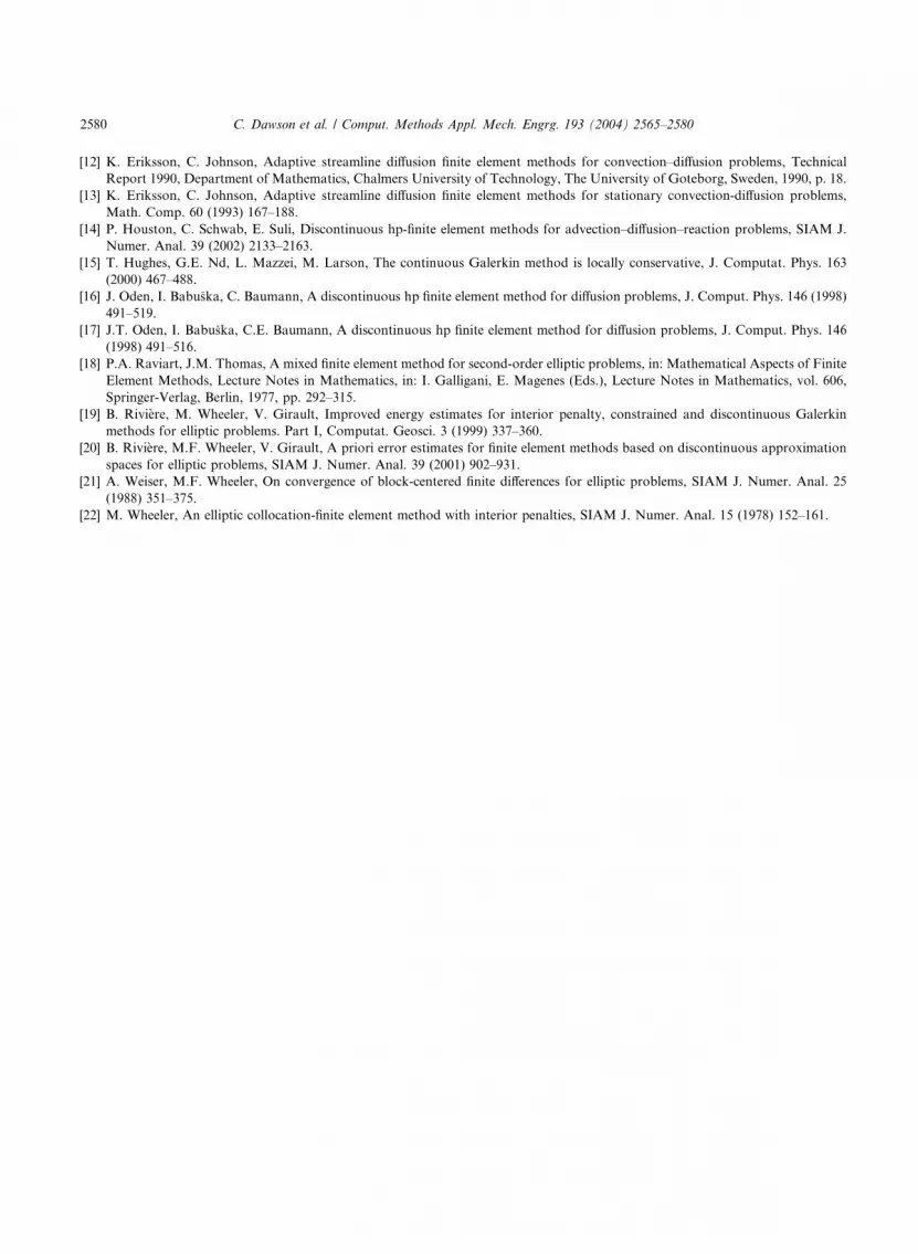
Fig. 8. Transport result from OBB based on flow result from OBB.
2578 C. Dawson et al. / Comput. Methods Appl. Mech. Engrg. 193 (2004) 2565–2580
The final example involves coupling OBB for transport with the IIPG method for flow (OBB–IIPG), andcomparing it to coupling OBB for flow with OBB for transport (OBB–OBB). We consider (3) and (39) on
the two-dimensional domain X ¼ ð0; 1Þ2. In this case, D and K are constant diagonal tensors with Dii ¼ 10:0and Kii ¼ 10:0. Initial concentration c0 and in-flow concentration cI are 1.0 uniformly. The flow boundary is
divided into CN ¼ ðf0g � ð0; 1ÞÞ [ ðð0; 1Þ � f1gÞ and CD ¼ oX n CN . The boundary pressure gD ¼ 0 on
ðð0; 1Þ � f0gÞ and gD ¼ 100 on ðf1g � ð0; 1ÞÞ. We know in this case that the exact solution is c � 1. The
simulation is run until time T ¼ 1, and backward Euler is used to march in time with Dt ¼ 0:01. A uniform
Fig. 9. Error of transport result from OBB based on flow result from OBB.
C. Dawson et al. / Comput. Methods Appl. Mech. Engrg. 193 (2004) 2565–2580 2579
16 · 16 mesh and the space of discontinuous piecewise polynomials of total degree two are used for solvingboth transport and flow. The penalty parameter in the IIPG method is chosen according to the formula
r ¼ r0r2K1=2=h, where r is the order of the local polynomial space, K is the scalar permeability, h is the
element size and r0 ¼ 1:0� 10�10.
The flow results from using the OBB and IIPG methods are shown in Figs. 6 and 7, respectively. The
velocity fields from the two methods seem to be quite similar. However, the transport result using the
velocity from the OBB method has a significant error (see Fig. 8 for the concentration profile at t ¼ 1 and
Fig. 9 for its error), while the transport result using the velocity from the IIPG method has no error up to
machine precision. Clearly, the property of zeroth-order accuracy of the combined OBB–IIPG methodresults in essentially no error in this example, and the violation of this property by the combined OBB–OBB
method results in significant error accumulation for concentration.
5. Conclusions
In this paper, we have examined the compatibility of various flow and transport methods, based on using
either continuous or discontinuous finite element methods. It was found that the SD method is alwayszeroth-order accurate whereas both the OBB and the LDG methods are always globally conservative for
transport, independent of how velocity is computed. The global conservation of the SD method and the
zeroth-order accuracy of the OBB and the LDG methods for transport hold only when a compatible
algorithm for flow is used. We have also shown that the LDG, the IIPG and the MFE methods for flow can
be compatible with the SD and the LDG methods for transport, under certain conditions. The NIPG, the
OBB and the SIPG for flow are not compatible with the SD and the LDG methods for transport. We have
demonstrated, through numerical examples, how incompatible methods may produce erroneous solutions,
or result in loss of mass. Though we have concentrated primarily on transport in porous media, the ideaspresented here extend to other application areas, including water quality modeling.
References
[1] V. Aizinger, C. Dawson, B. Cockburn, P. Castillo, Local discontinuous Galerkin methods for contaminant transport, Adv. Water
Resour. 24 (2000) 73–87.
[2] C.E. Baumann, J.T. Oden, A discontinuous hp finite element method for convection–diffusion problems, Comput. Methods Appl.
Mech. Engrg. 175 (1999) 311–341.
[3] R. Berger, S. Howington, Discrete fluxes and mass balance in finite elements, J. Hydraul. Engrg. 128 (2002) 87–92.
[4] A. Brooks, T. Hughes, Streamline upwind Petrov–Galerkin formulations for convection dominated flows with particular emphasis
on the incompressible Navier–Stokes equation, Comput. Meth. Appl. Mech. Engrg. 32 (1982) 199–259.
[5] P. Castillo, B. Cockburn, I. Perugia, D. Sch€otzau, An a priori error analysis of the local discontinuous Galerkin method for elliptic
problems, SIAM J. Numer. Anal. 38 (2000) 1676–1706.
[6] S. Chippada, C.N. Dawson, M.L. Mart�ınez, M.F. Wheeler, A projection method for constructing a mass conservative velocity
field, Comput. Meth. Appl. Mech. Engrg. 151 (1998) 1–10.
[7] B. Cockburn, C. Dawson, Some extensions of the local discontinuous Galerkin method for convection–diffusion equations in
multidimensions, in: J. Whiteman (Ed.), The Proceedings of the Conference on the Mathematics of Finite Elements and
Applications: MAFELAP X, Elsevier, Amsterdam, 2000.
[8] B. Cockburn, C. Shu, The local discontinuous Galerkin finite element method for convection–diffusion systems, SIAM J. Numer.
Anal. 35 (1998) 2440–2463.
[9] B. Cockburn, C.-W. Shu, The local discontinuous Galerkin method for time-dependent convection–diffusion systems, SIAM J.
Numer. Anal. 35 (1998) 2440–2463 (electronic).
[10] C. Dawson, Conservative, shock-capturing transport methods with nonconservative velocity approximations, Computat. Geosci.
3 (1999) 205–227.
[11] C.N. Dawson, S. Sun, M.F. Wheeler, Error estimates and performance for incomplete interior penalty Galerkin method (in
preparation).
2580 C. Dawson et al. / Comput. Methods Appl. Mech. Engrg. 193 (2004) 2565–2580
[12] K. Eriksson, C. Johnson, Adaptive streamline diffusion finite element methods for convection–diffusion problems, Technical
Report 1990, Department of Mathematics, Chalmers University of Technology, The University of Goteborg, Sweden, 1990, p. 18.
[13] K. Eriksson, C. Johnson, Adaptive streamline diffusion finite element methods for stationary convection-diffusion problems,
Math. Comp. 60 (1993) 167–188.
[14] P. Houston, C. Schwab, E. Suli, Discontinuous hp-finite element methods for advection–diffusion–reaction problems, SIAM J.
Numer. Anal. 39 (2002) 2133–2163.
[15] T. Hughes, G.E. Nd, L. Mazzei, M. Larson, The continuous Galerkin method is locally conservative, J. Computat. Phys. 163
(2000) 467–488.
[16] J. Oden, I. Babu�ska, C. Baumann, A discontinuous hp finite element method for diffusion problems, J. Comput. Phys. 146 (1998)
491–519.
[17] J.T. Oden, I. Babu�ska, C.E. Baumann, A discontinuous hp finite element method for diffusion problems, J. Comput. Phys. 146
(1998) 491–516.
[18] P.A. Raviart, J.M. Thomas, A mixed finite element method for second-order elliptic problems, in: Mathematical Aspects of Finite
Element Methods, Lecture Notes in Mathematics, in: I. Galligani, E. Magenes (Eds.), Lecture Notes in Mathematics, vol. 606,
Springer-Verlag, Berlin, 1977, pp. 292–315.
[19] B. Rivi�ere, M. Wheeler, V. Girault, Improved energy estimates for interior penalty, constrained and discontinuous Galerkin
methods for elliptic problems. Part I, Computat. Geosci. 3 (1999) 337–360.
[20] B. Rivi�ere, M.F. Wheeler, V. Girault, A priori error estimates for finite element methods based on discontinuous approximation
spaces for elliptic problems, SIAM J. Numer. Anal. 39 (2001) 902–931.
[21] A. Weiser, M.F. Wheeler, On convergence of block-centered finite differences for elliptic problems, SIAM J. Numer. Anal. 25
(1988) 351–375.
[22] M. Wheeler, An elliptic collocation-finite element method with interior penalties, SIAM J. Numer. Anal. 15 (1978) 152–161.
Related Documents