Comparison of Two Data Smoothing Techniques for Vegetation Spectra Derived From EO1 Hyperion

RESEARCH ARTICLE

Comparison of Two Data Smoothing Techniquesfor Vegetation Spectra Derived From EO-1 Hyperion

Anshu Miglani & Shibendu S. Ray &

D. P. Vashishta & Jai Singh Parihar

Received: 17 November 2008 /Accepted: 25 March 2011 /Published online: 10 June 2011# Indian Society of Remote Sensing 2011

Abstract Hyperspectral data are generally noisier com-pared to broadband multispectral data because theirnarrow bandwidth can only capture very little energythat may be overcome by the self-generated noise insidethe sensors. It is desirable to smoothen the reflectancespectra. This study was carried out to see the effect ofsmoothing algorithms - Fast-Fourier Transform (FFT)and Savitzky–Golay (SG) methods on the statisticalproperties of the vegetation spectra at varying filter sizes.The data used in the study is the reflectance spectra dataobtained from Hyperion sensor over an agriculturallydominated area in Modipuram (Uttar Pradesh). Thereflectance spectra were extracted for wheat crop atdifferent growth stages. Filter sizes were varied between3 and 15with the increment of 2. Paired t-test was carriedout between the original and the smoothed data for allthe filter sizes in order to see the extent of distortionwith changing filter sizes. The study showed that inFFT, beyond filter size 11, the number of locationswithin the spectra where the smooth spectra werestatistically different from its original counterpartincreased to 14 and reaches 21 at the filter size 15.

However, in SG method, number of statisticallydifferent locations were more than those found in theFFT, but the number of locations did not changingdrastically. The number of statistically disturbed loca-tions in SG method varied between 16 and 19. Theoptimum filter size for smoothing the vegetation spectrawas found to be 11 in FFT and 9 in SG method.

Keywords Hyperspectral . FFT. Savitzky–Golay .

Smoothing . Vegetation spectra . Noise

Introduction

One of the most important problems of using hyper-spectral data is low signal to noise level (Vaiphasa2006). Hyperspectral data covers the contiguousspectral range and has fine spectral resolution. Thespectra may thus include several unwanted andunattributed absorption peaks, which may lead to theincorporation of noise (error) into the data (Jensen etal. 2003). This is commonly called sensor systeminduced error. There are two reasons for the noise ―either narrow bandwidth can only capture very littleenergy/signal (usually occurs around 1,400, 1,900,and 2,500 nm and also at wavelength less that300 nm) or the signal can be overcome by the self-generated noise inside the sensors. Detectors miscali-bration, Sun’s variable illumination and atmosphericstates are some of the factors causing noise inside thesensor which decrease the precision of spectral signals

J Indian Soc Remote Sens (December 2011) 39(4):443–453DOI 10.1007/s12524-011-0103-5

Anshu Miglani is a former Research Fellow.

A. Miglani (*) : S. S. Ray : J. S. PariharABHG/EPSA, Space Applications Center, ISRO,Ahmedabad, Indiae-mail: [email protected]

D. P. VashishtaH. N. B., Garhwal University,Srinagar, Uttarakhand

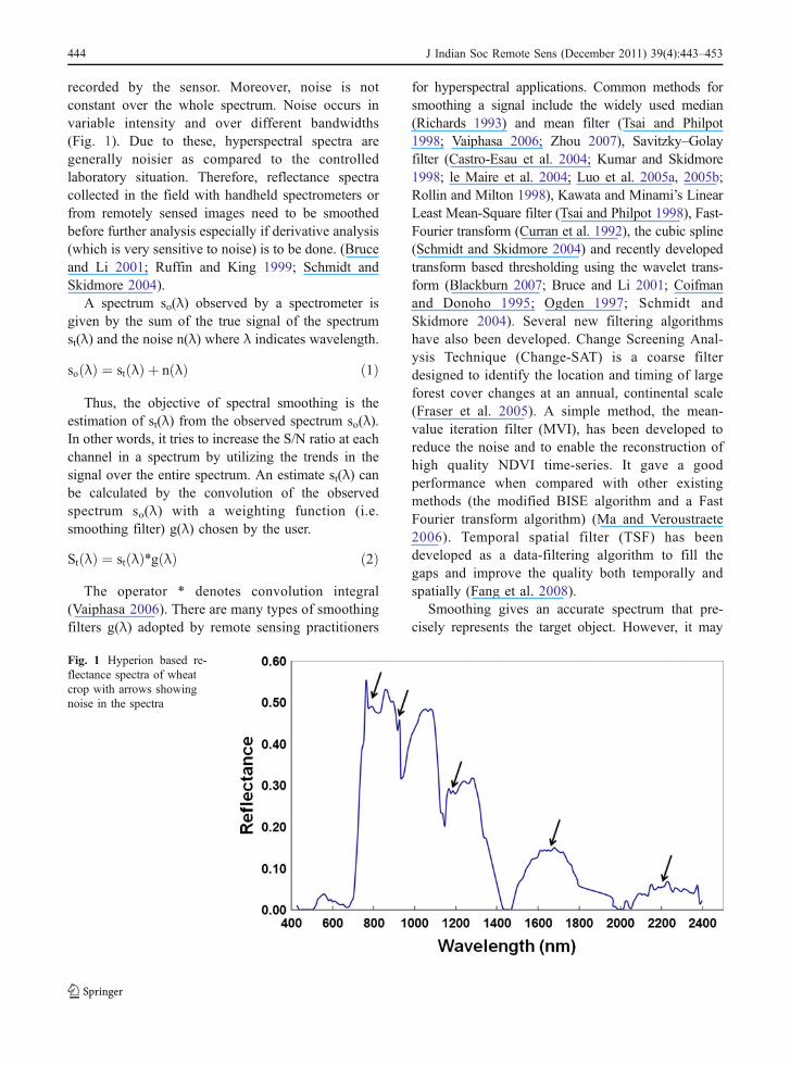
recorded by the sensor. Moreover, noise is notconstant over the whole spectrum. Noise occurs invariable intensity and over different bandwidths(Fig. 1). Due to these, hyperspectral spectra aregenerally noisier as compared to the controlledlaboratory situation. Therefore, reflectance spectracollected in the field with handheld spectrometers orfrom remotely sensed images need to be smoothedbefore further analysis especially if derivative analysis(which is very sensitive to noise) is to be done. (Bruceand Li 2001; Ruffin and King 1999; Schmidt andSkidmore 2004).

A spectrum so(λ) observed by a spectrometer isgiven by the sum of the true signal of the spectrumst(λ) and the noise n(λ) where λ indicates wavelength.

so λð Þ ¼ st λð Þ þ n λð Þ ð1Þ

Thus, the objective of spectral smoothing is theestimation of st(λ) from the observed spectrum so(λ).In other words, it tries to increase the S/N ratio at eachchannel in a spectrum by utilizing the trends in thesignal over the entire spectrum. An estimate st(λ) canbe calculated by the convolution of the observedspectrum so(λ) with a weighting function (i.e.smoothing filter) g(λ) chosen by the user.

St λð Þ ¼ st λð Þ»g λð Þ ð2Þ

The operator * denotes convolution integral(Vaiphasa 2006). There are many types of smoothingfilters g(λ) adopted by remote sensing practitioners

for hyperspectral applications. Common methods forsmoothing a signal include the widely used median(Richards 1993) and mean filter (Tsai and Philpot1998; Vaiphasa 2006; Zhou 2007), Savitzky–Golayfilter (Castro-Esau et al. 2004; Kumar and Skidmore1998; le Maire et al. 2004; Luo et al. 2005a, 2005b;Rollin and Milton 1998), Kawata and Minami’s LinearLeast Mean-Square filter (Tsai and Philpot 1998), Fast-Fourier transform (Curran et al. 1992), the cubic spline(Schmidt and Skidmore 2004) and recently developedtransform based thresholding using the wavelet trans-form (Blackburn 2007; Bruce and Li 2001; Coifmanand Donoho 1995; Ogden 1997; Schmidt andSkidmore 2004). Several new filtering algorithmshave also been developed. Change Screening Anal-ysis Technique (Change-SAT) is a coarse filterdesigned to identify the location and timing of largeforest cover changes at an annual, continental scale(Fraser et al. 2005). A simple method, the mean-value iteration filter (MVI), has been developed toreduce the noise and to enable the reconstruction ofhigh quality NDVI time-series. It gave a goodperformance when compared with other existingmethods (the modified BISE algorithm and a FastFourier transform algorithm) (Ma and Veroustraete2006). Temporal spatial filter (TSF) has beendeveloped as a data-filtering algorithm to fill thegaps and improve the quality both temporally andspatially (Fang et al. 2008).

Smoothing gives an accurate spectrum that pre-cisely represents the target object. However, it may

Fig. 1 Hyperion based re-flectance spectra of wheatcrop with arrows showingnoise in the spectra

444 J Indian Soc Remote Sens (December 2011) 39(4):443–453

cause changes to the original spectral data that couldlead to incorrect results in subsequent analyses. Plantbiophysical studies and vegetation discrimination andclassification are dependent on statistical estimates ofspectral data that are often dampened by smoothingfilters. Therefore it is very crucial to select the correctsmoothing method for a particular Hyperspectralapplication so as to minimize disturbance to theoriginal spectral data (Vaiphasa 2006). Followingrequirements have to be met by smoothing algorithms(Schmidt 2003).

▪ Absorption feature should be preserved whileremoving noise.

▪ Wavelength position of the local minima ormaxima as well as the inflection point should notbe removed. It means ability to resolve finespectral details as well as the noise removalcapacity should be well optimized in order tominimize disturbances to original spectral data(Ray et al. 2010).

▪ The algorithm should be computationally straightforward.

In other words, the trade-off between noiseremoval and the ability to resolve fine spectral detailshould be optimized towards preserving the spectraldetail.

In this context, this study was carried out with thefollowing objective:

▪ To study and compare the effect of the smoothingtechniques — Fast-Fourier Transform (FFT) andSavitzky–Golay (SG) methods- on the statisticalproperties of the vegetation spectra of wheat cropobtained from the space borne Hyperion onboardEO-1 at varying filter sizes.

▪ To propose the use of one statistical test (a pairedt-test) as a tool in order to see the extent ofdistortion with changing filter sizes.

Study Area

The study was conducted in Rohata block of Meerutdistrict (Central Coordinate: 29d00’ N and 77d36’ E,232 m above MSL) of Uttar Pradesh. Climate here istropical semi arid, with alluvial soil type. The area ishighly productive having mostly irrigated crops. Themajor crops during Rabi (winter) season include

wheat and sugarcane. The other minor crops includedpotato, mustard, berseem, sorghum etc.

Data Used

The data used for the present study is the reflectancespectra obtained from space borne EO-1 onboardHyperion sensor. Hyperion operates across the fullsolar reflected spectrum with nominal spectral cover-age from 400–2,500 nm (Green et al. 2003). Itacquires information both in visible-near infrared(VNIR 355.589–851.92 nm) and short wave infrared(SWIR 1057.36–2577.07 nm) region through twospectrometers and a single telescope (Datt et al.2003). The Hyperion has 70 bands in the VNIRsensor and 172 bands in the SWIR, providing, in all,242 wavebands with ~10 nm bandwidth, 30 m-ground resolution, 7.7 km swath, 16 days of temporalresolution for nadir viewing with 12 bits quantization(Green et al. 2003). Typically 198 bands wereprovided in the calibrated data. Since two out of 198bands were overlapping, we were left with 196 bandsin all, which were used for further studies.

Methodology

We studied the effect of several smoothing techniqueson vegetation spectra obtained from the satellite basedhyperspectral sensor. The pre-processing of Hyperiondata was carried out through i) digital number toradiance transformation and ii) atmospheric correc-tions and reflectance retrieval (Miglani et al. 2008).Spectral profiles of wheat crop at different growthstages viz. milking, booting, anthesis, grainfill andmaturity, were individually studied to analyze thespectral behaviors in narrow bands in terms ofreflectance. Training sites were marked for each ofthe class. These classes were chosen on the basis ofthe ground-truth collected during field observation.Mean values for each channel were computed foreach of these classes.

Smoothing

The reflectance data of wheat at the above mentionedstages were used in the Origin software (of Origin-Lab) for smoothing. Smoothing creates a function that

J Indian Soc Remote Sens (December 2011) 39(4):443–453 445

attempts to capture important patterns in the data,while leaving out noise (Vaiphasa 2006). Techniquesapplied for smoothing, included: Savitzky-Golay filterand Fast Fourier Transform. These two techniques aredescribed in detail in following sections.

Fast Fourier Transform (FFT) Filtering

A Fourier transform is a mathematical technique forseparating a single band of remotely sensed imageinto its various spatial frequency components.Because much of the noise associated with remote-ly sensed imagery is due to high-frequency striping,it is possible to use a Fourier transform to remove it(Jensen et al. 2003). FFTs were first discussed byCooley and Tukey (1965). Origin software was usedto carry out FFT filtering. This method is based onFFT low-pass filter. In essence, it removes the high-frequency components with a parabolic window.FFT is accomplished by removing Fourier compo-nents with frequencies higher than a cutoff frequency(eqn 3).

Fcutoff ¼ 1=nΔt ð3Þwhere, n is the number of data points specified bythe user, and Δt is the spacing between two adjacentdata points. Larger values of n result in lower cutofffrequencies, and thus a greater degree of smoothing.A value of zero for n leaves the data unsmoothed.

Savitzky–Golay (SG) Filter

SG filter is one of the very common smoothingtechniques used in hyperspectral remote sensing. Itcan be thought of as a weighted moving average,where the filter coefficients are derived by performingan unweighed linear least squares fit using a polyno-mial of given order (Savitzky and Golay 1964). It isbased on the mathematical deduction of the leastsquares approximation over equally spaced wave-length intervals. The general equation of the simpli-fied least square convolution can be represented asfollows:

Yj» ¼X

CiYjþ1=N ð4Þ

Where Y is the original spectrum, Y* is theresultant (smoothed) spectrum, Ci is the coefficientfor the ith spectral value of the filter (smoothing

window), and N is the number of convolutingintegers. The index j is the running index of originalordinate data table. The smoothing array (filter size)consists of 2m + 1 points, where m is the half-widthof the smoothing window (Tsai and Philpot 1998).

It gives a visibly smoother appearance. SG filter isused in many near infrared spectroscopy studies andtherefore has also been adopted for hyperspectralremote sensing studies. This method shifts theposition of the spectral features and creates artifactsat discontinuities in the spectrum. This methodperforms well on the sections of the spectrum awayfrom sharp discontinuities in reflectance, but it has thedisadvantage of smoothing at these discontinuities(Schmidt and Skidmore 2004).

SG was found to give a better result than meanfilter on the basis of statistical characteristics of thespectral data (Tsai and Philpot 1998; Vaiphasa 2006).It was found that moving average filters statisticallydisturbed the original spectral response more than SGfilters as the number of statistically different locationswere higher in mean filter. The general trends of bothmoving average and SG filters indicated that biggerfilter sizes resulted in higher statistical disturbances(Vaiphasa 2006).

Filter Size

For smoothing FFT and SG methods were used for allthe test sites. This was carried for all the wavelengthsranging between 426 and 2,395 nm. Filter sizes werevaried between 3 and 15 in FFT and 5 to 13 in case ofSG method with the increment of 2 (i.e. 3, 5,7……….15).

Evaluation of Two Filters and their Filter Sizes

The effect of the smoothing techniques was testedby comparing smoothed spectra to the originalspectra visually and on the basis of RMSE. RMSEwas evaluated for major absorption or reflectancepeaks, i.e. Green Maxima, Red Minima and NIRMaxima as well as for different regions of thespectrum, for all the filter sizes used in FFT and SGmethod. This was done

▪ to find out which filter is performing better for thevegetation spectra under study and

▪ to optimize the filter size.

446 J Indian Soc Remote Sens (December 2011) 39(4):443–453

We also studied the wavelength position andreflectance of selected local minima and maxima, inorder to detect the shift in the spectral features due tothe smoothing technique and quantify it throughRMSE with respect to the original spectra.

The smoothed data of all filter sizes was statisti-cally compared against the original dataset usingpaired t-test. The numbers of spectral bands that havep-values less that 0.05 were recorded for every filter.This was done to find out the number of statistically

different locations, where smoothed spectra is differ-ent from the original spectra.

Results and Discussion

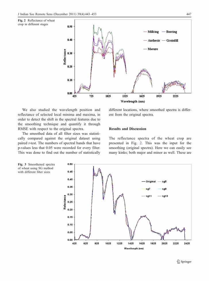
The reflectance spectra of the wheat crop arepresented in Fig. 2. This was the input for thesmoothing (original spectra). Here we can easily seemany kinks; both major and minor as well. These are

Fig. 2 Reflectance of wheatcrop in different stages

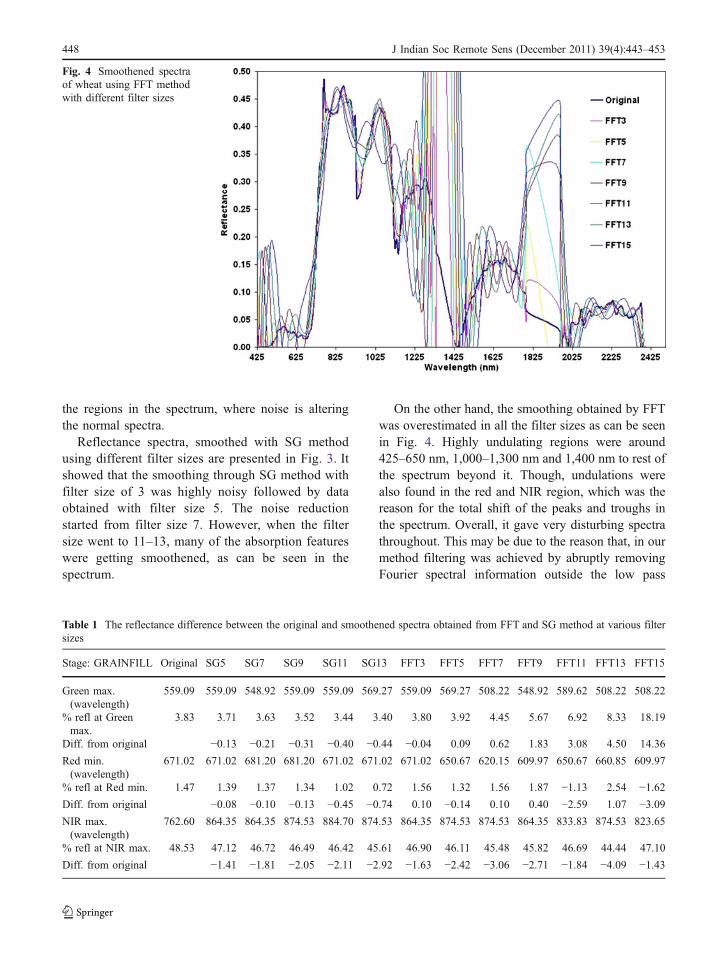
Fig. 3 Smoothened spectraof wheat using SG methodwith different filter sizes

J Indian Soc Remote Sens (December 2011) 39(4):443–453 447

the regions in the spectrum, where noise is alteringthe normal spectra.

Reflectance spectra, smoothed with SG methodusing different filter sizes are presented in Fig. 3. Itshowed that the smoothing through SG method withfilter size of 3 was highly noisy followed by dataobtained with filter size 5. The noise reductionstarted from filter size 7. However, when the filtersize went to 11–13, many of the absorption featureswere getting smoothened, as can be seen in thespectrum.

On the other hand, the smoothing obtained by FFTwas overestimated in all the filter sizes as can be seenin Fig. 4. Highly undulating regions were around425–650 nm, 1,000–1,300 nm and 1,400 nm to rest ofthe spectrum beyond it. Though, undulations werealso found in the red and NIR region, which was thereason for the total shift of the peaks and troughs inthe spectrum. Overall, it gave very disturbing spectrathroughout. This may be due to the reason that, in ourmethod filtering was achieved by abruptly removingFourier spectral information outside the low pass

Fig. 4 Smoothened spectraof wheat using FFT methodwith different filter sizes

Table 1 The reflectance difference between the original and smoothened spectra obtained from FFT and SG method at various filtersizes

Stage: GRAINFILL Original SG5 SG7 SG9 SG11 SG13 FFT3 FFT5 FFT7 FFT9 FFT11 FFT13 FFT15

Green max.(wavelength)

559.09 559.09 548.92 559.09 559.09 569.27 559.09 569.27 508.22 548.92 589.62 508.22 508.22

% refl at Greenmax.

3.83 3.71 3.63 3.52 3.44 3.40 3.80 3.92 4.45 5.67 6.92 8.33 18.19

Diff. from original −0.13 −0.21 −0.31 −0.40 −0.44 −0.04 0.09 0.62 1.83 3.08 4.50 14.36

Red min.(wavelength)

671.02 671.02 681.20 681.20 671.02 671.02 671.02 650.67 620.15 609.97 650.67 660.85 609.97

% refl at Red min. 1.47 1.39 1.37 1.34 1.02 0.72 1.56 1.32 1.56 1.87 −1.13 2.54 −1.62Diff. from original −0.08 −0.10 −0.13 −0.45 −0.74 0.10 −0.14 0.10 0.40 −2.59 1.07 −3.09NIR max.(wavelength)

762.60 864.35 864.35 874.53 884.70 874.53 864.35 874.53 874.53 864.35 833.83 874.53 823.65

% refl at NIR max. 48.53 47.12 46.72 46.49 46.42 45.61 46.90 46.11 45.48 45.82 46.69 44.44 47.10

Diff. from original −1.41 −1.81 −2.05 −2.11 −2.92 −1.63 −2.42 −3.06 −2.71 −1.84 −4.09 −1.43

448 J Indian Soc Remote Sens (December 2011) 39(4):443–453

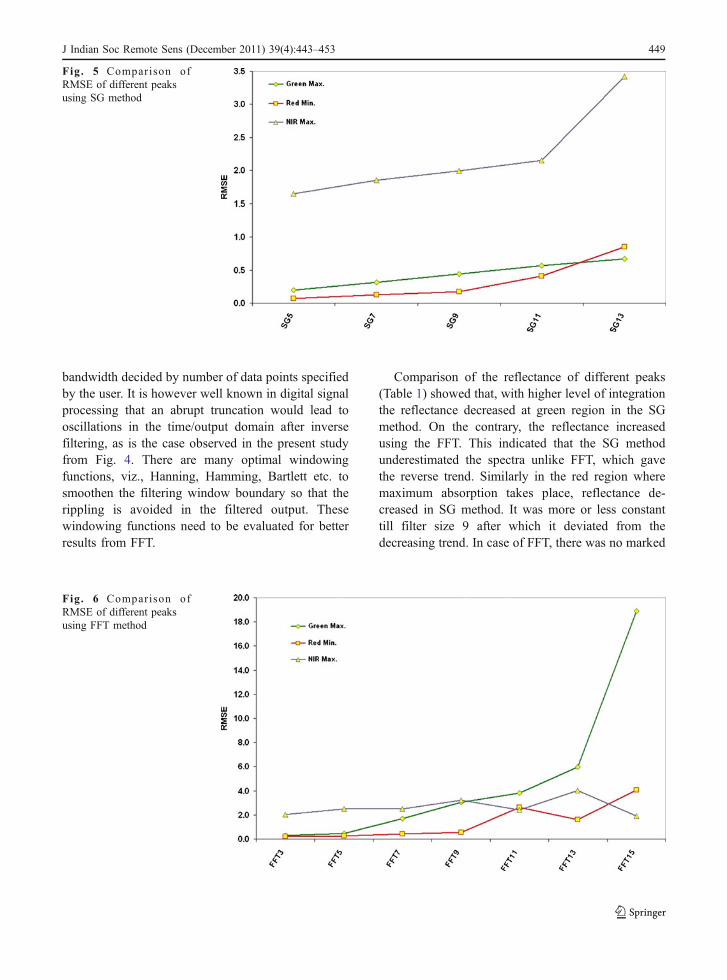
bandwidth decided by number of data points specifiedby the user. It is however well known in digital signalprocessing that an abrupt truncation would lead tooscillations in the time/output domain after inversefiltering, as is the case observed in the present studyfrom Fig. 4. There are many optimal windowingfunctions, viz., Hanning, Hamming, Bartlett etc. tosmoothen the filtering window boundary so that therippling is avoided in the filtered output. Thesewindowing functions need to be evaluated for betterresults from FFT.

Comparison of the reflectance of different peaks(Table 1) showed that, with higher level of integrationthe reflectance decreased at green region in the SGmethod. On the contrary, the reflectance increasedusing the FFT. This indicated that the SG methodunderestimated the spectra unlike FFT, which gavethe reverse trend. Similarly in the red region wheremaximum absorption takes place, reflectance de-creased in SG method. It was more or less constanttill filter size 9 after which it deviated from thedecreasing trend. In case of FFT, there was no marked

Fig. 5 Comparison ofRMSE of different peaksusing SG method

Fig. 6 Comparison ofRMSE of different peaksusing FFT method

J Indian Soc Remote Sens (December 2011) 39(4):443–453 449

trend, which was followed at the red minima and NIRmaxima.

RMSE was computed for all the filter sizes used inSG method and FFT techniques for Green, Red andNIR reflectance (Fig. 5 & Fig. 6). Figure 5 shows thatmaximum RMSE was found in the NIR region usingSG method. It gradually increased with the increase inthe filter size and abruptly increased at the filter size13. Negligible increase in RMSE was found in thegreen and red region. This showed that the impact ofsmoothing was most noticeable in the NIR regionfollowed by red and green regions. Except in thegreen region, no obvious pattern was found in FFT(Fig. 6). This is also depicted in the Table 1. In caseof green maxima, RMSE markedly increased (fromthe value 0.44 to 5.44). The increase became abrupt atfilter size 15 as it reached the value of 17.39. In redminima, the increase was small and gradual till filtersize 9, after which it lost the trend. RMSE values inthe NIR region were maximum from the filter size 3till 9. High reflectance in the NIR region was due tothe presence of intercellular spaces within the leaves,which caused internal light scattering (Horler et al.1983). Reflectance values in this region are helpful inpredicting the plant health status. That is why it isvery crucial to optimize the filter size especially if thetarget spectrum is of vegetation. We may notice, outof three reflectance, NIR maximum was the mostaffected peak by both SG method (at all filter sizes)and FFT (till filter size 9). If we compare among thetwo methods, it was always SG method whichprovided lesser RMSE than FFT.

We not only compared the inflection points i.e.Green maxima, red minima and NIR maxima, but alsocompared the effect of smoothing on different regionsof the spectrum. We also tried to find out whichregions were least sensitive to the smoothing. Table 2shows the regions whose RMSE was less than 0.01 atthe filter sizes being used during FFT and SG method.RMSE obtained from SG method shows that thevisible region (400–700 nm) along with 1,200–1,300 nm, 1,500–1,800 nm and 2,100–2,200 nm werethe ones which were most resistant to changes due tosmoothing. Howsoever, 800–900 nm region waspreserved till filter size 11 and 1,000–1,100 nm tillfilter size 9. 1,900–2,100 nm region was highlydisturbed by the smoothing effect. It indicated thatfilter size 11 was optimum for the vegetation spectrasince all the major regions, in which vegetation T

able

2Spectralregion

swith

RMSE<0.01

obtained

atvaryingfiltersizesusingSG

metho

dandFFT

SG-5

SG-7

SG-9

SG-11

SG-13

FFT3

FFT5

FFT7

FFT9

FFT11

FFT13

FFT15

400–50

040

0–50

040

0–50

040

0–50

040

0–50

050

1–60

060

1–70

060

1–70

021

01–2

200

2201–2

300

2201

–230

0

501–60

050

1–60

050

1–60

050

1–60

050

1–60

060

1–70

080

1–90

016

01–1

700

2201

–230

0

601–70

060

1–70

060

1–70

060

1–70

060

1–70

080

1–90

010

01–110

021

01–2

200

801–90

080

1–90

080

1–90

080

1–90

012

01–1

300

1001–110

015

01–1

600

2201–2

300

1001

–110

010

01–110

010

01–110

012

01–1

300

1501

–160

015

01–1

600

1601

–170

0

1201

–130

012

01–1

300

1201

–130

015

01–1

600

1601

–170

016

01–1

700

2101

–220

0

1501

–160

015

01–1

600

1501

–160

016

01–1

700

1701

–180

021

01–2

200

2201

–230

0

1601

–170

016

01–1

700

1601

–170

017

01–1

800

2101

–220

022

01–2

300

1701

–180

017

01–1

800

1701

–180

021

01–2

200

2201

–230

0

1901

–200

021

01–2

200

2101

–220

022

01–2

300

2001

–210

022

01–2

300

2201

–230

0

2101

–220

0

2201

–230

0

450 J Indian Soc Remote Sens (December 2011) 39(4):443–453

showed its characteristic signature, were preserved.Even the water absorption features (at around 900,1,100 & 1,400 nm) were also maintained. On theother hand, FFT caused high disturbances in thespectra, may be due to the reason described earlier.2,200–2,300 nm (which is of not much significancefor green vegetation) was the only region, which waspreserved till filter size 13. 500–900 nm region waspreserved till filter size 3 and 600–900 nm till 5. Outof this red region was the most stable region, whichcould be preserved till filter size 7.

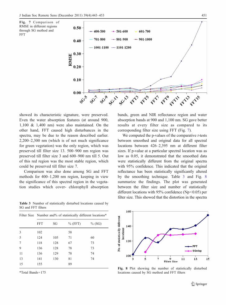
Comparison was also done among SG and FFTmethods for 400–1,200 nm region, keeping in viewthe significance of this spectral region in the vegeta-tion studies which cover- chlorophyll absorption

bands, green and NIR reflectance region and waterabsorption bands at 900 and 1,100 nm. SG gave betterresults at every filter size as compared to itscorresponding filter size using FFT (Fig. 7).

We computed the p-values of the comparative t-testsbetween smoothed and original data for all spectrallocations between 426–2,395 nm at different filtersizes. If p-value at a particular spectral location was aslow as 0.05, it demonstrated that the smoothed datawere statistically different from the original spectrawith 95% confidence. This indicated that the originalreflectance has been statistically significantly alteredby the smoothing technique. Table 3 and Fig. 8summarize the findings. The plot was generatedbetween the filter size and number of statisticallydifferent locations with 95% confidence (Np<0.05) perfilter size. This showed that the distortion in the spectra

Fig. 7 Comparison ofRMSE in different regionsthrough SG method andFFT

Table 3 Number of statistically disturbed locations caused bySG and FFT filters

Filter Size Number and% of statistically different locations*

FFT SG % (FFT) % (SG)

3 102 58

5 124 105 71 60

7 118 128 67 73

9 136 128 78 73

11 136 129 78 74

13 141 130 81 74

15 155 89

*Total Bands=175Fig. 8 Plot showing the number of statistically disturbedlocations caused by SG method and FFT filters

J Indian Soc Remote Sens (December 2011) 39(4):443–453 451

started increasing with the filter size. In similar filtersizes SG techniques resulted less number of statistical-ly disturbed locations than FFT method.

Conclusion

The study showed that, hyperspectral data smoothingshould be used taking into consideration optimumfilter size, which causes minimal disturbances to theoriginal data. Comparative RMSE was proposed as ameasure for choosing the best smoothing filter for thehyperspectral data. Standard destriping techniquesuch as the FFT-filtering was not able to produce areasonable result. However SG method seemed to bemore promising for spectra smoothing. Filter size 7 to11 for SG method was found to be optimum forvegetation studies on the basis of RMSE.

Acknowledgement Authors are grateful to Sushma Pani-grahy, Group Director, ABHG/EPSA for her critical sugges-tions for improvement.

References

Blackburn, G. A. (2007). Wavelet decomposition of hyper-spectral reflectance data for quantifying photosyntheticpigment concentrations in Vegetation. Journal of Experi-mental Botany, 58(4), 855–867.

Bruce, L. M., & Li, L. (2001). Wavelets for computionallyefficient hyperspectral derivative analysis. I.E.E.E.Transactions on Geoscience and Remote Sensing, 39,2001.

Castro-Esau, K. L., Sánchez-Azofeifa, G. A., & Caelli, T.(2004). Discrimination of lianas and trees with leaf-levelhyperspectral data. Remote Sensing of Environment, 90(15), 353–372.

Coifman, R. R., & Donoho, D. L. (1995). Translation invariantde-noising. In A. A. Antoniadis & G. Oppenheim (Eds.),Wavelets and Statistics (pp. 125–150). New York: Spring-er Verlag. Vol. 103 of Lecture Notes in Statistics.

Cooley, J. W., & Tukey, O. W. (1965). An algorithm for themachine calculation of complex fourier series. Mathemat-ics of Computation, 19, 297–301.

Curran, P. J., Dungan, J. L., Macler, B. A., Plummer, S. E.,& Peterson, D. L. (1992). Reflectance spectroscopy offresh whole leaves for the estimation of chemicalconcentration. Remote Sensing of Environment, 39,153–166.

Datt, B., McVicar, T. R., Van Niel, T. G., Jupp, D. L. B., &Pearlman, J. S. (2003). Preprocessing EO-1 Hyperionhyperspectral data support the application of agricultural

indexes. I.E.E.E. Transactions on Geoscience and RemoteSensing, 41, 1246–1259.

Fang, H., Liang, S., Townshend, J. R., & Dickinson, R. E.(2008). Spatially and temporally continuous LAI data setsbased on an integrated filtering method: examples fromNorth America. Remote Sensing of Environment, 112(15),75–93.

Fraser, R. H., Abuelgasim, A., & Latifovic, R. (2005). Amethod for detecting large-scale forest cover change usingcoarse spatial resolution imagery. Remote Sensing ofEnvironment, 95(4), 414–427.

Green, R. O., Pavri, B. E., & Chrien, T. G. (2003). On orbitradiometric and spectral calibration characteristics of EO-1hyperion derieved with an underflight of AVIRIS and Insitu measurements at Salar de Arizaro. Argentina RemSens of Envir, 41, 1194–1203.

Horler, D. N. H., Dockray, M. and Barber J. (1983). The red-edge of plant reflectance. International Journal of RemoteSensing, 4, 273–288.

Jensen, J. R., Hadley, B. C., Tullis, J. A., Gladden, J., Nelson,E., Riley, S., Filippi, T. and Pendergast, M. (2003). 2002Hyperspectral Analysis of Hazardous Waste Sites on TheSavannah River Site. WSRC-TR-2003-00275. Preparedfor the U.S. Department of Energy Under ContractNumber DE-AC09-96SR18500.

Kumar, L. and Skidmore, A. K. (1998). Use of derivativespectroscopy to identify regions of difference betweensome Australian eucalypt species. 9th Australasian Re-mote Sensing and Photogrammetry Conference, Sydney,Australia.

le Maire, G., François, C., & Dufrêne, E. (2004). Towardsuniversal broad leaf chlorophyll indices using PROS-PECT simulated database and hyperspectral reflectancemeasurements. Remote Sensing of Environment, 89(1),1–28.

Luo, J., Ying, K., He, P., & Bai, J. (2005a). Savitzky–Golaysmoothing and differentiation filter for even number data.Signal Processing, 85(7), 1429–1434.

Luo, J., Ying, K., He, P., & Bai, J. (2005b). Properties ofSavitzky–Golay digital differentiators. Digital SignalProcessing, 15, 122–136.

Ma, M., & Veroustraete, F. (2006). Reconstructing pathfind-er AVHRR land NDVI time-series data for the North-west of China. Advances in Space Research, 37, 835–840.

Miglani, A., Ray, S. S., Pandey, R., & Parihar, J. S. (2008).Evaluation and pre-processing of EO-1 Hyperion data foragricultural applications. Journal of the Indian Society ofRemote Sensing, 36, 255–266.

Ogden, R. T. (1997). Essential wavelets for statistical applica-tions and data analysis. Boston: Birkhauser.

Ray, S. S., Jain, N., Miglani, A., Singh, J. P., Singh, A. K.,Panigrahy, S., et al. (2010). Defining optimum spectralnarrow bands and band-widths for agricultural applica-tions. Current Science, 98, 1365–1369.

Richards, J. A. (1993). Remote sensing digital image analysis:An introduction (2nd ed.). Berlin: Springer.

Rollin, E. M., & Milton, E. J. (1998). Processing of highspectral resolution reflectance data for the retrieval ofcanopy water content information. Remote Sensing ofEnvironment, 65, 86–92.

452 J Indian Soc Remote Sens (December 2011) 39(4):443–453

Ruffin, C., and King, R.L. (1999) The analysis of hyperspectraldata using Savitzky-Golay filtering- Theoretical basis(Part-I). Presented in: Geoscience and Remote SensingSymposium, 1999. IGARSS '99 Proceedings. IEEE 1999International, Vol. 2: 756–758

Savitzky, A., & Golay, M. J. E. (1964). Smoothing anddifferentiation of data by simplified least squares proce-dures. Analytical Chemistry, 36, 1627–1639.

Schmidt, K.S. (2003). Hyperspectral Remote Sensing ofVegetation Species Distribution in a Saltmarsh. ISBN90-5808-830-8, ITC Dissertation number 96, Interna-tional Institute For Geo-Information Science And EarthObservation, Enschede, The Netherlands.

Schmidt, K. S., & Skidmore, A. K. (2004). Smoothingvegetation spectra with wavelets. International Journalof Remote Sensing, 25, 1167–1184.

Tsai, F., & Philpot, W. (1998). Derivative analysis ofhyperspectral data. Remote Sensing of Environment, 66,41–51.

Vaiphasa, C. (2006). Consideration of smoothing techniques forhyperspectral remote sensing. ISPRS Journal of Photo-grammetry and Remote Sensing, 60, 91–99.

Zhou, B. (2007). Application of Hyperspectral Remote SensingIn Detecting and Mapping Sericea Lespedeza in Missouri.M.A. Thesis Presented to The Faculty of the GraduateSchool University of Missouri-Columbia

J Indian Soc Remote Sens (December 2011) 39(4):443–453 453