Comparison of top-down and bottom-up estimates of sectoral and regional greenhouse gas emission reduction potentials

Page 1

ARTICLE IN PRESS

Energy Policy 37 (2009) 5125–5139

Contents lists available at ScienceDirect

Energy Policy

0301-42

doi:10.1

� Corr

E-m

journal homepage: www.elsevier.com/locate/enpol

Comparison of top-down and bottom-up estimates of sectoral and regionalgreenhouse gas emission reduction potentials

Detlef P. van Vuuren a,�, Monique Hoogwijk b, Terry Barker c, Keywan Riahi d, Stefan Boeters e,Jean Chateau f, Serban Scrieciu c, Jasper van Vliet a, Toshihiko Masui g, Kornelis Blok b,Eliane Blomen b, Tom Kram a

a Netherlands Environmental Assessment Agency, PO Box 303, 3720 AH Bilthoven, The Netherlandsb ECOFYS Netherlands BV, The Netherlandsc Cambridge University, UKd IIASA, Austriae Netherlands Bureau for Economic Policy Analysis, The Netherlandsf Organisation for Economic Co-operation and Development, Franceg National Institute for Environmental Studies, Japan

a r t i c l e i n f o

Article history:

Received 27 April 2009

Accepted 21 July 2009Available online 13 August 2009

Keywords:

Emission reduction potential

Energy models

Top-down models

15/$ - see front matter & 2009 Elsevier Ltd. A

016/j.enpol.2009.07.024

esponding author. Tel.: +3130 2742046.

ail address: [email protected] (D.P. van

a b s t r a c t

The Fourth Assessment Report of IPCC reports that greenhouse gas emissions can be reduced by about

30–50% in 2030 at costs below 100 US$/tCO2 based on an assessment of both bottom-up and top-down

studies. Here, we have looked in more detail into the outcomes of specific models and also analyzed the

economic potentials at the sectoral and regional level. At the aggregated level, the findings of the IPCC

report are confirmed. However, substantial differences are found at the sectoral level. At the same time,

there seems to be no systematic difference in the reduction potential reported by top-down and

bottom-up approaches. The largest reduction potential as a response to carbon prices exists in the

energy supply sector. Reduction potential in the building sector may carry relatively low costs. Although

uncertainties are considerable, the modeling results and the bottom-up analyses all suggest that at the

global level around 50% of greenhouse gas emissions may be reduced at carbon price (costs) below

100$/tCO2-eq—but with a wide range of 30–60%. At a carbon price (costs) less than 20$/tCO2-eq, still

10–35% of emissions may be abated. The variation of results is higher at low carbon-price levels than at

high levels.

& 2009 Elsevier Ltd. All rights reserved.

1. Introduction

The amount of greenhouse gas emissions that can be avoidedat costs below a certain level plays a key role in climate policyanalysis. Estimates of economic reduction potentials (the amountof greenhouse gas emissions that can be reduced at different costslevels) are, however, complicated by uncertainty in severaldimensions: uncertainty about the costs of different technologiesand their development over time and uncertainty about theinteraction of the energy sector with the rest of the economy(Weyant, 2000). A wide range of models has been developed thattreat these aspects of uncertainty in different ways and provideinsights into emission reduction potentials under their respectiveassumptions. The models are developed from various scientificparadigms, which may lead to different interpretations of the

ll rights reserved.

Vuuren).

past and different expectations of the future (Rotmans and deVries, 1997). A main cleavage is between models that are rootedeither in a macro-economic tradition (top-down) or in anengineering tradition (bottom-up) (Grubb et al., 1993; Hourcadeand Shukla, 2001; Loschel, 2002). In brief, a typical top-downapproach focuses on market interactions within the wholeeconomy and has little technological detail in the energy sector.A typical bottom-up approach focuses on the substitutability ofindividual energy technologies and their relative costs (see alsoSection 2). In the past, considerable attention has been paid tothe different outcomes of these two modelling traditions, inparticular to lower cost levels and higher reduction potentialsoften found in bottom-up studies. However, there is alsoconsiderable variation in results within each tradition. Recently,an increasing number of hybrid models have emerged, whichaim at combining the advantages of both perspectives bylinking macro-economic and technology model components(e.g. MESSAGE-MACRO, Messner and Schrattenholzer, 2000; seealso Hourcade et al., 2006).

Page 2

ARTICLE IN PRESS

D.P. van Vuuren et al. / Energy Policy 37 (2009) 5125–51395126

IPCC’s Fourth Assessment Report (AR4) assessed the 2030emission reduction potential at different cost levels based oninformation from both top-down and bottom-up studies (IPCC,2007). One important conclusion was that the full mitigationpotential needed to limit greenhouse gas concentrations in thelong-run to 450 ppm CO2-eq would be available at costs below100 US$/tCO2 (in this article we use 2000 US$). Remarkably, theglobal emission reduction potentials from bottom-up and top-down approaches were very similar (including the uncertaintyranges). Still, at the sectoral level considerable differenceswere found. The IPCC report, however, also admitted that lackof consistency across studies could hinder the interpretationof these results. The bottom-up results, for instance, werebased on assessments of individual studies with very differentbaselines. The top-down results were derived from a statisticalanalysis of a range of different studies (using different targets andbaselines).

Given the interest of policy-makers in emission reductionpotentials (among others as input to the negotiations as part ofthe United Nations Framework Convention on Climate Change),the IPCC numbers have received considerable attention and theirrobustness has become an important issue. In the current study,we aim to obtain a deeper understanding of the emissionreduction potentials as assessed by IPCC by performing a moresystematic comparison between top-down and bottom-up modeloutcomes. Specifically, we focus on two questions: (1) are theeconomic potentials as reported by IPCC correct, and (2) can weexplain the differences between the different models andmethods? These questions are tackled by running coordinatedsimulations using a set of selected models (see Section 2). Theresults are compared to results from a parallel study, in which theIPCC bottom-up analysis was updated (Hoogwijk et al., 2008). Thishas two main advantages: We can systematically discuss theuncertainty ranges between the different models and modellingapproaches and we can represent the sectoral information moreconsistently than in the IPCC assessment.

The article is structured as follows. First we discuss methodo-logical issues, including a brief introduction to different modellingapproaches and a description of the simulations that havebeen performed. Next, we discuss the results of the modelcomparison vis-�a-vis the new estimates from bottom-up studiesand the original IPCC results. Finally, we draw conclusions withrespect to the economic potential of reducing greenhouse gasemissions and associated uncertainty and we provide recommen-dations that would allow a better assessment in subsequent IPCCreports.

2. Methodological issues in model comparison studies

2.1. Different types of reduction potentials

The amount of greenhouse gas emissions that can be reducedis often referred to as the (technical or economic) emissionreduction potential. It should be noted, however, that the exactdefinition of these potentials varies in literature and that it is infact hard to define them unambiguously across different types ofmodels and studies. In the IPCC report, the term ‘‘technicalpotential’’ is defined as the total amount of avoided greenhousegas emissions as a result of implementation of reductionmeasures (by sector or economy-wide) while still providing asimilar level of service (based on Halsnæs et al., 2007). Thetechnical reduction potential is (in principle) not limited by costconstraints, but by practical and physical limits, such as thenumber of available technologies and the rate at which thesetechnologies may be employed. The term economic potential, in

contrast, refers to the quantity of greenhouse gas emissions thatcan be reduced at given costs compared to a reference (based onHalsnæs et al., 2007). The economic potential therefore takes intoaccount both costs and technical limits, and is thus generallysmaller than the technical potential. The term ‘‘economicpotential’’ is typically defined from a macro-economic perspectiveusing a social discount rate. Mitigation potentials that have beencalculated using the discount rates of private actors are referred toas ‘‘market potentials’’. In case of model studies the distinctionbecomes less clear as empirically derived relationships in modelsmay be based on the discount rates that were actually applied atthat time. Implementation of measures also depends onother barriers such as non-optimal responses or lack of informa-tion. Typically, for equilibrium-based, top-down, technology-focused studies, these factors will not be part of the economicreduction potential. It should, however, be noted again thatthe concepts are somewhat ambiguous when applied tomodel results. Using, for example, historically derived priceelasticities as a basis to describe substitution, implies that price-responsive barriers of the past are implicitly included in themodel as well, which makes a distinction between economicpotential and actual implementation rather difficult. Theseconsiderations are important to interpret the various studies inliterature.

2.2. Different types of models

In assessing long-term energy-system trends and the costs ofachieving policy targets different model approaches exist. Animportant distinction can be made between bottom-up and top-down models. Obviously, in reality this distinction is not clear-cut,but part of a range or variations.

2.2.1. Bottom-up and top-down approaches

The typical bottom-up approach looks at how a number ofindividual energy technologies can be used (and substituted) inorder to provide energy services (Loschel, 2002). Substitution isbased on relative costs, which is in turn driven by factors such asthe technology development. The typical bottom-up approachfocuses on the energy system itself and not on the relationshipwith the economy as a whole. In many bottom-up approaches, thecurrent energy system is not necessarily assumed to be optimal.Therefore, analysts tend to find that currently several cost-efficient technologies are not used due to implementationbarriers—and low-costs improvements can be made by usingthese technologies. Bottom-up tools range from the basictechnology databases with relatively simple implementation tomodels with more system information such as MARKAL (seeoverview provided by Worrell et al., 2004).

The typical top-down model approach focuses on the economyas a whole and describes substitution across different inputs onthe basis of historically calibrated factors. The focus is on marketprocesses rather than technology detail. Also within this group,different approaches exist, including computable general-equili-brium models (CGE), econometric models and also more hybrid,process-oriented models, which they combine technology detailand more general descriptions of economic processes.

The fact that the distinction between the top-down andbottom-up approach is not very clear-cut implies that somemodels could actually be easily included in both categories. TheIPCC AR4 report, for instance, uses the term top-down for nearlyall integrated modeling approaches—while the term bottom-up isused for the assessment of reduction potential based on individualtechnologies. Here, we follow the same distinction since the aim

Page 3

ARTICLE IN PRESS

D.P. van Vuuren et al. / Energy Policy 37 (2009) 5125–5139 5127

of this study is to further investigate the reduction potentials asreported by IPCC.

The economic potential to reduce greenhouse gas emissionscan be determined in bottom-up studies by introducing differentgreenhouse gas emission reduction measures in the order of theircosts (cheapest measure first)—and next adding up the totalreduction potential of measures with costs below a certain level. Ifdone properly, the costs of more expensive measures will be(negatively) influenced by the measures already taken earlier inthe cost-function—and an attempt is made to avoid doublecounting of efficiency and energy supply measures. In top-downmodels, economic potentials are estimated by running modelsalong a pre-described carbon-price path.1

2.2.2. The role of optimization

Optimization is used in both bottom-up and top-down models.Optimization leads to a ‘‘preferred’’ mix of technologies (orallocation of production factors) vis-�a-vis a chosen optimizationtarget (e.g. lowest costs or maximum private consumption) givencertain constraints (e.g. tax levels). In case a model uses optimiza-tion also to develop the model baseline, i.e. development in theabsence of climate policy, introduction of perturbation (e.g. pricingemitting greenhouse gases) will automatically lead to a non-optimal situation. An alternative, however, is not to use optimiza-tion but instead describe the economy or energy system on thebasis of a set of rules that do not necessarily lead to such fullequilibrium (simulation models). In that case, perturbation maylead to model outcomes with even lower costs (or a higherconsumption level). This distinction is important to understandwhy certain approaches may have negative costs (some technology-oriented studies) or increased income levels. Most models will notapply full optimization. For instance, in CGE models optimization istypically constrained by exogenous factors such as tax levels—andthere is no inter-temporal optimization. Still it is very unlikely thatclimate policy would lead to negative costs in these models.

2.2.3. Strengths and weaknesses of different approaches

In the past, several studies have focused on the question whybottom-up studies reported larger reduction potential than top-down studies, with part of this potential at negative costs. Grubbet al. (1993) concentrated on the different assumptions of theoptimality of past and future energy systems (see Section 2.2.2),indicating that the negative reduction potential in the bottom-upapproach originates from the difference between the currentposition and the technology frontier. In recent years, thedistinction between the approaches has been reduced and thestrengths and weaknesses of both approaches are better recog-nized (Hourcade et al., 2006; Hourcade and Shukla, 2001).Bottom-up models bring in more energy-system detail andinsights into the technology development and allow evaluatinga wider range of policy options. Disadvantages include the lack ofmacro-economic feedbacks between the energy and othereconomic sectors, such as energy price-induced changes ofmacro-economic production and consumption. Top-down modelsadd a larger economic context and the associated interactions(feedbacks and spillovers), use a more comprehensive costsconcept (i.e. income loss for the total economy versus costs forthe energy system only), and the baseline scenario is most of thetime consistently developed within the model. Disadvantages ofthis approach are that, as model calibration factors (elasticities)

1 One could argue that this ‘‘model response’’ does not necessarily reflect an

economic potential—as in some models implementation barriers are accounted

for, but for simplicity throughout the article we will use the term economic

potential.

are determined on the basis of historic evidence, historic behavioris assumed to be relevant for future systems as well. By definition,representation of specific technologies and other physical para-meters is poor, which makes it difficult to analyse other policiesthan introducing emission prices. As mentioned further above,this dichotomy between the bottom-up and top-down approacheshas been bridged in an increasing number of models. Also ourstudy includes a few of these hybrid models, including the multi-sector version of the MESSAGE-MACRO model (Rao and Riahi,2006).

2.3. Comparison approach in the IPPC Fourth Assessment Report

One of the tasks of the IPCC AR4 was to provide estimates ofemission reduction potentials at various cost levels. The ability forIPCC authors to assess these was complicated by the fact that theauthors had to build upon a diverse set of studies with verydifferent assumptions. Partly in response to this, the assessmentwas separated into two categories, assessing the bottom-up andtop-down literature.

The bottom-up assessment was organized around sector-specific studies run by author teams, who collected availableliterature in order to derive sectoral reduction potentials. Thesector information was aggregated into economy-wide potentialswhile correcting for overlap (see Hoogwijk et al., 2008; IPCC,2007). On the top-down side, the IPCC-assessment team collectedcombinations of carbon prices and associated greenhouse gasemission reductions in 2030 of previously published studies asincluded in scenario databases and model comparison studies(Edenhofer et al., 2006; Hanaoka et al., 2006; Nakicenovic et al.,2006; Weyant et al., 2007).

Despite the considerable work that was done, the IPCCauthors were not able to discuss the underlying information indetail. Important reasons for this included the mandate ofthe IPCC, i.e. assessment, not research, and limitations in timeof the authors. This has led, specifically, to the followinglimitations:

�

The sector teams in the bottom-up assessment used slightlydifferent methods to assess available literature despite regularmeetings to harmonize methods. This includes the way theliterature was interpreted to account for differences in base-lines and discount rates. � In the top-down assessment, the studies taken into account in

the statistical analysis all used very different baselines,emission reduction targets, type of models, etc. For mostsectors, still a statistically relevant relationship was found.However there was little insight in the underlying causes of theuncertainty range around this relationship. For instance, thecarbon-price trajectories between the studies differed con-siderably, but its influence could not be tested.

� Comparison between the bottom-up and top-down informa-

tion was basically constrained to the global potential at variouscosts levels. Very little attention was paid to the underlyingsectoral data or to the methodological differences that maycause inconsistencies.

2.4. Comparison approach in this paper

This study adds to the original IPCC analysis in two differentways:

�

First, in addition to the IPCC bottom-up assessment, weuse here the updated bottom-up assessment published byHoogwijk et al. (2008). This study represents a bottom-up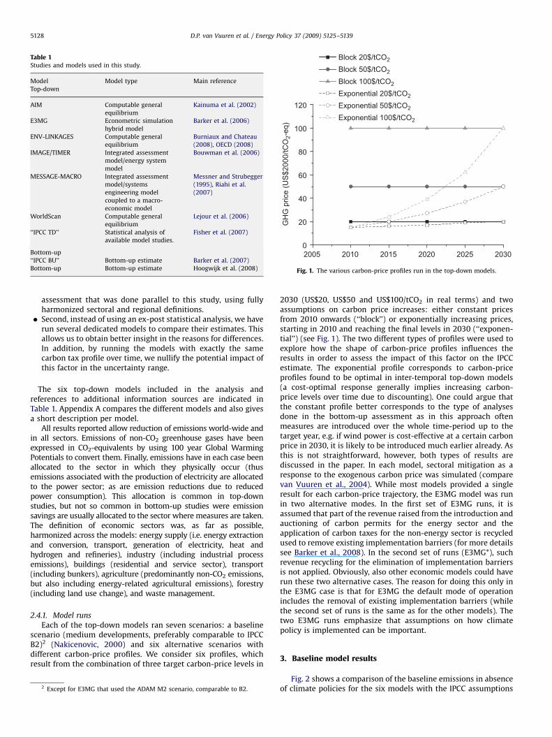

Page 4

ARTICLE IN PRESS

Table 1Studies and models used in this study.

Model Model type Main reference

Top-down

AIM Computable general

equilibrium

Kainuma et al. (2002)

E3MG Econometric simulation

hybrid model

Barker et al. (2006)

ENV-LINKAGES Computable general

equilibrium

Burniaux and Chateau

(2008), OECD (2008)

IMAGE/TIMER Integrated assessment

model/energy system

model

Bouwman et al. (2006)

MESSAGE-MACRO Integrated assessment

model/systems

engineering model

coupled to a macro-

economic model

Messner and Strubegger

(1995), Riahi et al.

(2007)

WorldScan Computable general

equilibrium

Lejour et al. (2006)

‘‘IPCC TD’’ Statistical analysis of

available model studies.

Fisher et al. (2007)

Bottom-up

‘‘IPCC BU’’ Bottom-up estimate Barker et al. (2007)

Bottom-up Bottom-up estimate Hoogwijk et al. (2008)

20050

20

40

60

80

100

120

GH

G p

rice

(US

$200

0/tC

O2-

eq)

Block 20$/tCO2

Block 50$/tCO2

Block 100$/tCO2

Exponential 20$/tCO2

Exponential 50$/tCO2

Exponential 100$/tCO2

2010 2015 2020 2025 2030

Fig. 1. The various carbon-price profiles run in the top-down models.

D.P. van Vuuren et al. / Energy Policy 37 (2009) 5125–51395128

assessment that was done parallel to this study, using fullyharmonized sectoral and regional definitions.

� Second, instead of using an ex-post statistical analysis, we have

run several dedicated models to compare their estimates. Thisallows us to obtain better insight in the reasons for differences.In addition, by running the models with exactly the samecarbon tax profile over time, we nullify the potential impact ofthis factor in the uncertainty range.

The six top-down models included in the analysis andreferences to additional information sources are indicated inTable 1. Appendix A compares the different models and also givesa short description per model.

All results reported allow reduction of emissions world-wide andin all sectors. Emissions of non-CO2 greenhouse gases have beenexpressed in CO2-equivalents by using 100 year Global WarmingPotentials to convert them. Finally, emissions have in each case beenallocated to the sector in which they physically occur (thusemissions associated with the production of electricity are allocatedto the power sector; as are emission reductions due to reducedpower consumption). This allocation is common in top-downstudies, but not so common in bottom-up studies were emissionsavings are usually allocated to the sector where measures are taken.The definition of economic sectors was, as far as possible,harmonized across the models: energy supply (i.e. energy extractionand conversion, transport, generation of electricity, heat andhydrogen and refineries), industry (including industrial processemissions), buildings (residential and service sector), transport(including bunkers), agriculture (predominantly non-CO2 emissions,but also including energy-related agricultural emissions), forestry(including land use change), and waste management.

2.4.1. Model runs

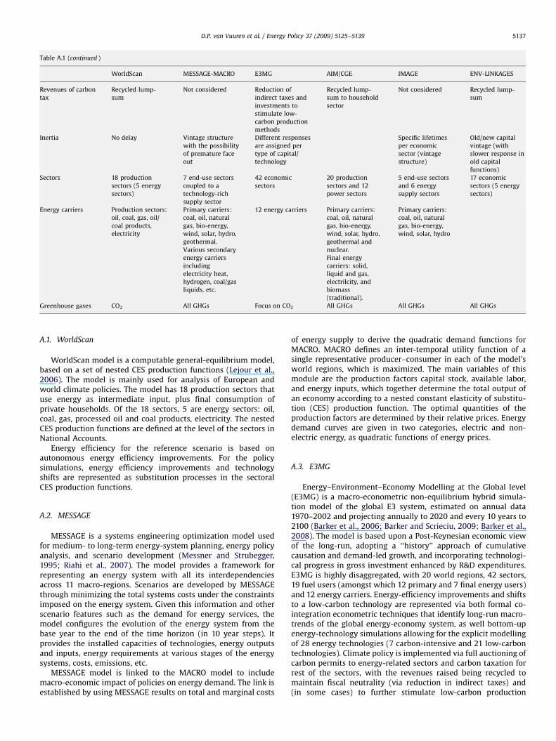
Each of the top-down models ran seven scenarios: a baselinescenario (medium developments, preferably comparable to IPCCB2)2 (Nakicenovic, 2000) and six alternative scenarios withdifferent carbon-price profiles. We consider six profiles, whichresult from the combination of three target carbon-price levels in

2 Except for E3MG that used the ADAM M2 scenario, comparable to B2.

2030 (US$20, US$50 and US$100/tCO2 in real terms) and twoassumptions on carbon price increases: either constant pricesfrom 2010 onwards (‘‘block’’) or exponentially increasing prices,starting in 2010 and reaching the final levels in 2030 (‘‘exponen-tial’’) (see Fig. 1). The two different types of profiles were used toexplore how the shape of carbon-price profiles influences theresults in order to assess the impact of this factor on the IPCCestimate. The exponential profile corresponds to carbon-priceprofiles found to be optimal in inter-temporal top-down models(a cost-optimal response generally implies increasing carbon-price levels over time due to discounting). One could argue thatthe constant profile better corresponds to the type of analysesdone in the bottom-up assessment as in this approach oftenmeasures are introduced over the whole time-period up to thetarget year, e.g. if wind power is cost-effective at a certain carbonprice in 2030, it is likely to be introduced much earlier already. Asthis is not straightforward, however, both types of results arediscussed in the paper. In each model, sectoral mitigation as aresponse to the exogenous carbon price was simulated (comparevan Vuuren et al., 2004). While most models provided a singleresult for each carbon-price trajectory, the E3MG model was runin two alternative modes. In the first set of E3MG runs, it isassumed that part of the revenue raised from the introduction andauctioning of carbon permits for the energy sector and theapplication of carbon taxes for the non-energy sector is recycledused to remove existing implementation barriers (for more detailssee Barker et al., 2008). In the second set of runs (E3MG*), suchrevenue recycling for the elimination of implementation barriersis not applied. Obviously, also other economic models could haverun these two alternative cases. The reason for doing this only inthe E3MG case is that for E3MG the default mode of operationincludes the removal of existing implementation barriers (whilethe second set of runs is the same as for the other models). Thetwo E3MG runs emphasize that assumptions on how climatepolicy is implemented can be important.

3. Baseline model results

Fig. 2 shows a comparison of the baseline emissions in absenceof climate policies for the six models with the IPCC assumptions

Page 5

ARTICLE IN PRESS

2000

WorldS

can

MESSAGEE3M

G

AIM/C

GE

IMAGE

ENV-Link

age

Bottom

-up

IPCC-T

D0

20

40

60

80

2000

MESSAGEE3M

G

AIM/C

GE

IMAGE

ENV-Link

age

Bottom

-up

IPCC-T

D0

20

40

60

80Energy CO2

Em

issi

ons

(GtC

O2-

eq)

Total

Waste Forestry Agriculture Industry Buildings Transport Energy supply

Total emissions

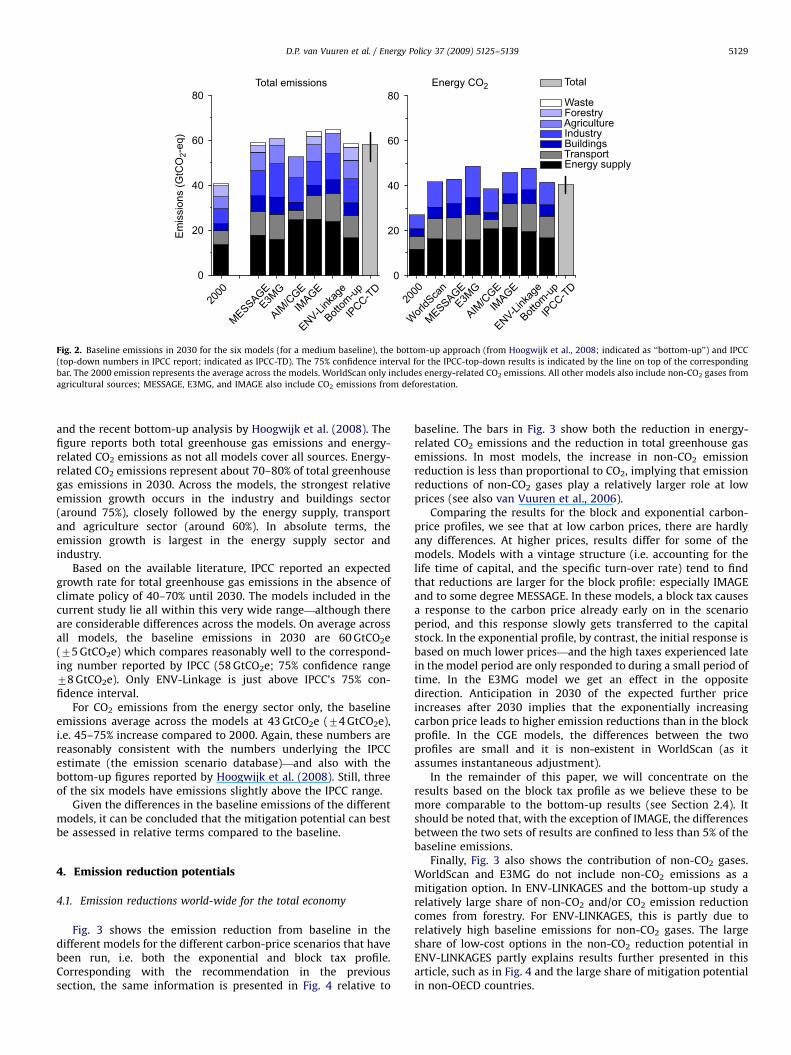
Fig. 2. Baseline emissions in 2030 for the six models (for a medium baseline), the bottom-up approach (from Hoogwijk et al., 2008; indicated as ‘‘bottom-up’’) and IPCC

(top-down numbers in IPCC report; indicated as IPCC-TD). The 75% confidence interval for the IPCC-top-down results is indicated by the line on top of the corresponding

bar. The 2000 emission represents the average across the models. WorldScan only includes energy-related CO2 emissions. All other models also include non-CO2 gases from

agricultural sources; MESSAGE, E3MG, and IMAGE also include CO2 emissions from deforestation.

D.P. van Vuuren et al. / Energy Policy 37 (2009) 5125–5139 5129

and the recent bottom-up analysis by Hoogwijk et al. (2008). Thefigure reports both total greenhouse gas emissions and energy-related CO2 emissions as not all models cover all sources. Energy-related CO2 emissions represent about 70–80% of total greenhousegas emissions in 2030. Across the models, the strongest relativeemission growth occurs in the industry and buildings sector(around 75%), closely followed by the energy supply, transportand agriculture sector (around 60%). In absolute terms, theemission growth is largest in the energy supply sector andindustry.

Based on the available literature, IPCC reported an expectedgrowth rate for total greenhouse gas emissions in the absence ofclimate policy of 40–70% until 2030. The models included in thecurrent study lie all within this very wide range—although thereare considerable differences across the models. On average acrossall models, the baseline emissions in 2030 are 60 GtCO2e(75 GtCO2e) which compares reasonably well to the correspond-ing number reported by IPCC (58 GtCO2e; 75% confidence range78 GtCO2e). Only ENV-Linkage is just above IPCC’s 75% con-fidence interval.

For CO2 emissions from the energy sector only, the baselineemissions average across the models at 43 GtCO2e (74 GtCO2e),i.e. 45–75% increase compared to 2000. Again, these numbers arereasonably consistent with the numbers underlying the IPCCestimate (the emission scenario database)—and also with thebottom-up figures reported by Hoogwijk et al. (2008). Still, threeof the six models have emissions slightly above the IPCC range.

Given the differences in the baseline emissions of the differentmodels, it can be concluded that the mitigation potential can bestbe assessed in relative terms compared to the baseline.

4. Emission reduction potentials

4.1. Emission reductions world-wide for the total economy

Fig. 3 shows the emission reduction from baseline in thedifferent models for the different carbon-price scenarios that havebeen run, i.e. both the exponential and block tax profile.Corresponding with the recommendation in the previoussection, the same information is presented in Fig. 4 relative to

baseline. The bars in Fig. 3 show both the reduction in energy-related CO2 emissions and the reduction in total greenhouse gasemissions. In most models, the increase in non-CO2 emissionreduction is less than proportional to CO2, implying that emissionreductions of non-CO2 gases play a relatively larger role at lowprices (see also van Vuuren et al., 2006).

Comparing the results for the block and exponential carbon-price profiles, we see that at low carbon prices, there are hardlyany differences. At higher prices, results differ for some of themodels. Models with a vintage structure (i.e. accounting for thelife time of capital, and the specific turn-over rate) tend to findthat reductions are larger for the block profile: especially IMAGEand to some degree MESSAGE. In these models, a block tax causesa response to the carbon price already early on in the scenarioperiod, and this response slowly gets transferred to the capitalstock. In the exponential profile, by contrast, the initial response isbased on much lower prices—and the high taxes experienced latein the model period are only responded to during a small period oftime. In the E3MG model we get an effect in the oppositedirection. Anticipation in 2030 of the expected further priceincreases after 2030 implies that the exponentially increasingcarbon price leads to higher emission reductions than in the blockprofile. In the CGE models, the differences between the twoprofiles are small and it is non-existent in WorldScan (as itassumes instantaneous adjustment).

In the remainder of this paper, we will concentrate on theresults based on the block tax profile as we believe these to bemore comparable to the bottom-up results (see Section 2.4). Itshould be noted that, with the exception of IMAGE, the differencesbetween the two sets of results are confined to less than 5% of thebaseline emissions.

Finally, Fig. 3 also shows the contribution of non-CO2 gases.WorldScan and E3MG do not include non-CO2 emissions as amitigation option. In ENV-LINKAGES and the bottom-up study arelatively large share of non-CO2 and/or CO2 emission reductioncomes from forestry. For ENV-LINKAGES, this is partly due torelatively high baseline emissions for non-CO2 gases. The largeshare of low-cost options in the non-CO2 reduction potential inENV-LINKAGES partly explains results further presented in thisarticle, such as in Fig. 4 and the large share of mitigation potentialin non-OECD countries.

Page 6

ARTICLE IN PRESS

0

10

20

30

40

50

Low

ENV-LINKAGES

IMAGE

AIM/C

GE

E3MG*

E3MG

WorldS

can

Em

issi

on re

duct

ion

(GtC

O2)

Expo-100 US$/tCO2 Block-100 US$/tCO2 Expo-50 US$/tCO2 Block-20 US$/tCO2 Expo-20 US$/tCO2 Block-20 US$/tCO2

MESSAGE High

Bottom Up

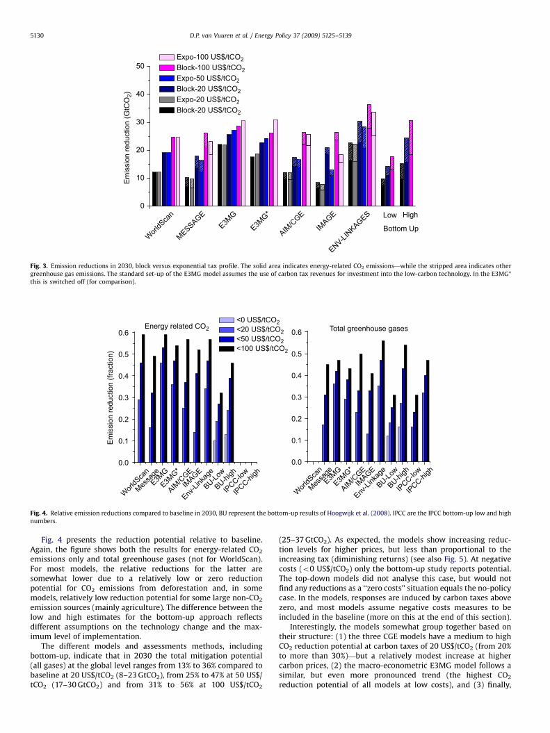
Fig. 3. Emission reductions in 2030, block versus exponential tax profile. The solid area indicates energy-related CO2 emissions—while the stripped area indicates other

greenhouse gas emissions. The standard set-up of the E3MG model assumes the use of carbon tax revenues for investment into the low-carbon technology. In the E3MG*

this is switched off (for comparison).

WorldS

can

Messa

geE3M

G

E3MG*

AIM/C

GE

IMAGE

Env-Li

nkag

e

BU-Low

BU-high

IPCC-lo

w

IPCC-hi

gh0.0

0.1

0.2

0.3

0.4

0.5

0.6Energy related CO2

WorldS

can

Messa

geE3M

G

E3MG*

AIM/C

GE

IMAGE

Env-Li

nkag

e

BU-Low

BU-high

IPCC-lo

w

IPCC-hi

gh0.0

0.1

0.2

0.3

0.4

0.5

0.6 Total greenhouse gases

Em

issi

on re

duct

ion

(frac

tion)

<0 US$/tCO2 <20 US$/tCO2 <50 US$/tCO2 <100 US$/tCO2

Fig. 4. Relative emission reductions compared to baseline in 2030, BU represent the bottom-up results of Hoogwijk et al. (2008). IPCC are the IPCC bottom-up low and high

numbers.

D.P. van Vuuren et al. / Energy Policy 37 (2009) 5125–51395130

Fig. 4 presents the reduction potential relative to baseline.Again, the figure shows both the results for energy-related CO2

emissions only and total greenhouse gases (not for WorldScan).For most models, the relative reductions for the latter aresomewhat lower due to a relatively low or zero reductionpotential for CO2 emissions from deforestation and, in somemodels, relatively low reduction potential for some large non-CO2

emission sources (mainly agriculture). The difference between thelow and high estimates for the bottom-up approach reflectsdifferent assumptions on the technology change and the max-imum level of implementation.

The different models and assessments methods, includingbottom-up, indicate that in 2030 the total mitigation potential(all gases) at the global level ranges from 13% to 36% compared tobaseline at 20 US$/tCO2 (8–23 GtCO2), from 25% to 47% at 50 US$/tCO2 (17–30 GtCO2) and from 31% to 56% at 100 US$/tCO2

(25–37 GtCO2). As expected, the models show increasing reduc-tion levels for higher prices, but less than proportional to theincreasing tax (diminishing returns) (see also Fig. 5). At negativecosts (o0 US$/tCO2) only the bottom-up study reports potential.The top-down models did not analyse this case, but would notfind any reductions as a ‘‘zero costs’’ situation equals the no-policycase. In the models, responses are induced by carbon taxes abovezero, and most models assume negative costs measures to beincluded in the baseline (more on this at the end of this section).

Interestingly, the models somewhat group together based ontheir structure: (1) the three CGE models have a medium to highCO2 reduction potential at carbon taxes of 20 US$/tCO2 (from 20%to more than 30%)—but a relatively modest increase at highercarbon prices, (2) the macro-econometric E3MG model follows asimilar, but even more pronounced trend (the highest CO2

reduction potential of all models at low costs), and (3) finally,

Page 7

ARTICLE IN PRESS

500

5

10

15

20

25

30

35

40

45

50

500

5

10

15

20

25

30

35

40

45

50

Red

uctio

ns (G

tCO

2-eq

)

Carbon tax ($/tCO2)

IPCC IPCC-IAM IPCC-CGE IPCC-linear corr

Carbon tax ($/tCO2)

This study WorldScan MESSAGE E3MG AIM/CGE IMAGE ENV-Linkages bottom-up (low/high)

100 100

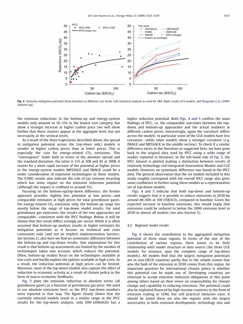
Fig. 5. Emission mitigation potential (from baseline) at different cost levels. Left statistical analysis as used for AR4. Right results of 6 models, and Hoogwijk et al. (2008)

(bottom-up).

D.P. van Vuuren et al. / Energy Policy 37 (2009) 5125–5139 5131

the emission reductions in the bottom-up and energy-systemmodels only amount to 10–15% in the lowest cost category, butshow a stronger increase at higher carbon price (we will showfurther that these clusters appear at the aggregate level, but notnecessarily at the sectoral level).

As a result of the three trajectories described above, the spreadin mitigation potential across the (top-down only) models issmaller at higher carbon prices than at lower prices. This isespecially the case for energy-related CO2 emissions. This‘‘convergence’’ holds both in terms of the absolute spread andthe standard deviation; the latter is 11% at 20$ and 4% at 100$. Areason for a more rapid increase of the potential at higher pricesin the energy-system models MESSAGE and IMAGE could be awider consideration of expensive technologies in these models.The E3MG results also indicate the role of tax revenue recyclingwhich has some impact on the emission reduction potential(although the impact is confined to around 5%).

Focusing on the bottom-up/top-down difference, the formerapproach provides slightly less potential at low prices—andcomparable estimates at high prices for total greenhouse gases.For energy-related CO2 emissions only, the bottom-up range liesmostly below the range of top-down model results. For totalgreenhouse gas emissions, the results of the two approaches arecomparable—consistent with the IPCC findings. Below, it will beshown that this result differs strongly per sector. While it is oftenassumed that bottom-up analysis results in higher estimates formitigation potentials as it focuses on technical and costsconstraints only (and not on implicit implementation barriers;see Section 2), also here we find no systematic difference betweenthe bottom-up and top-down results. One explanation for thisresult is that bottom-up assessments are limited by the number oftechnologies taken into account, which reduces the potential.Often, bottom-up studies focus on the technologies available atlow costs and hardly explore the options available at high costs. Asa result, the reduction potential at high prices can be limited.Moreover, most of the top-down models also capture the effect ofreduction in economic activity as a result of climate policy in theform of macro-economic feedbacks.

Fig. 5 plots the emission reduction in absolute terms (allgreenhouse gases) as a function of greenhouse gas price. We needto use absolute emissions here; as the IPCC top-down numberswere reported in that way. The figure clearly shows that thecurrently selected models result in a similar range as the IPCCresults for the top-down analysis; only ENV-LINKAGES has a

higher reduction potential. Both Figs. 4 and 5 confirm the mainfindings of IPCC, i.e. the comparable outcomes between the top-down and bottom-up approaches and the actual numbers atdifferent carbon prices. Interestingly, again the curvature differsacross the models: in particular some of the CGE models have lesscurvature—while other models show a stronger curvature (e.g.IMAGE and MESSAGE in the middle section). To check if a similardifference exists in the literature as suggested here, we have goneback to the original data used by IPCC using a wide range ofstudies reported in literature. In the left-hand side of Fig. 5, theIPCC dataset is plotted making a distinction between results ofrelatively technology-rich Integrated Assessment Models and CGEmodels. However, no systematic difference was found in the IPCCdata. The general observation that the six models included in thisstudy roughly correspond with the overall IPCC range also givessome confidence in further using these models as a representativeset of top-down models.

Figs. 4 and 5 indicate that both top-down and bottom-upresults suggest that it is possible to reduce emissions in 2030 byaround 40–60% at 100 US$/tCO2 compared to baseline. Given theexpected increase in baseline emissions, this would imply thatemissions could be reduced to below the 2000 emission level in2030 in almost all models (see also Section 5).

4.2. Regional model results

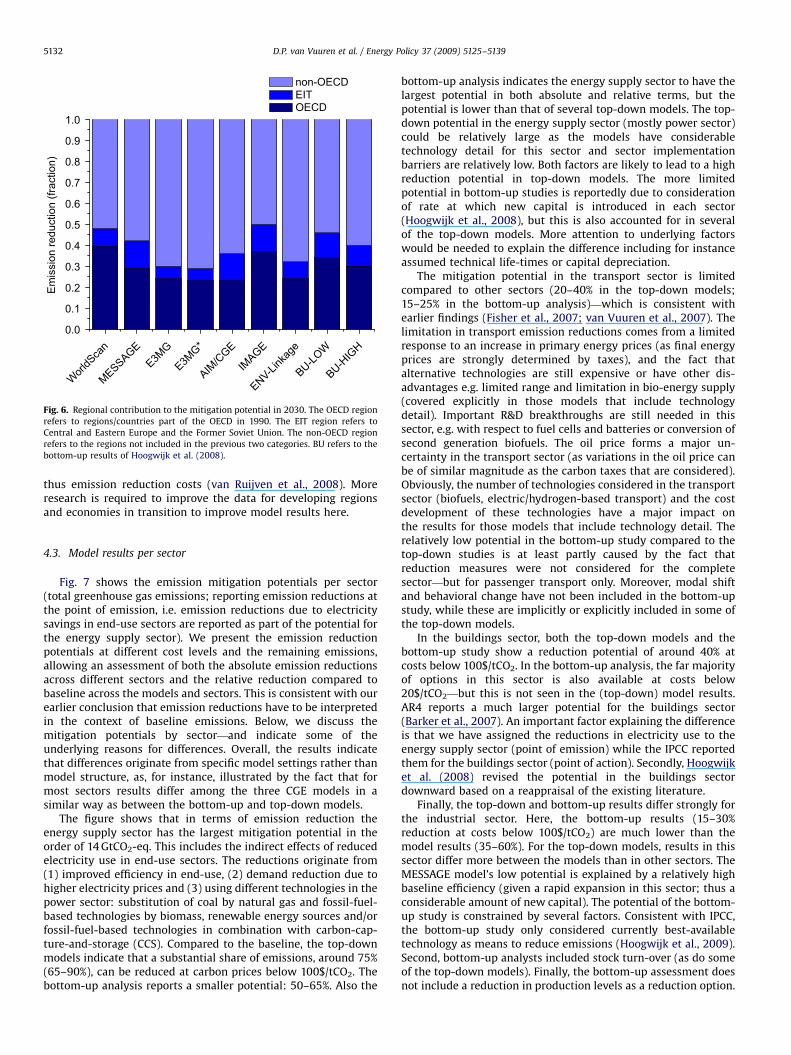
Fig. 6 shows the contribution to the aggregated mitigationpotential of three main regions. In terms of the size of thecontribution of various regions, there seems to be littlerelationship with model structure or data source (the three CGEmodels, for instance, span the complete range of top-downmodels). All models find that the largest mitigation potentialsare in non-OECD countries partly due to the simple reason thatalso the bulk of the emission in 2030 comes from this region. Animportant question for international climate policy is whetherthis potential can be made use of. Developing countries arereluctant to accept emission reduction obligations at this pointamong others based on their views on responsibility for climatechange and capability in reducing emissions. The potential couldalso be exploited financed by high-income countries in the form ofemission trading or CDM, but still practical obstacles exist. Itshould be noted these are also the regions with the largestuncertainty in both emission development, technology mix and

Page 8

ARTICLE IN PRESS

WorldS

can

MESSAGEE3M

G

E3MG*

AIM/C

GE

IMAGE

ENV-Link

age

BU-LOW

BU-HIG

H

0.0

0.1

0.2

0.3

0.4

0.5

0.6

0.7

0.8

0.9

1.0

Em

issi

on re

duct

ion

(frac

tion)

non-OECD EIT OECD

Fig. 6. Regional contribution to the mitigation potential in 2030. The OECD region

refers to regions/countries part of the OECD in 1990. The EIT region refers to

Central and Eastern Europe and the Former Soviet Union. The non-OECD region

refers to the regions not included in the previous two categories. BU refers to the

bottom-up results of Hoogwijk et al. (2008).

D.P. van Vuuren et al. / Energy Policy 37 (2009) 5125–51395132

thus emission reduction costs (van Ruijven et al., 2008). Moreresearch is required to improve the data for developing regionsand economies in transition to improve model results here.

4.3. Model results per sector

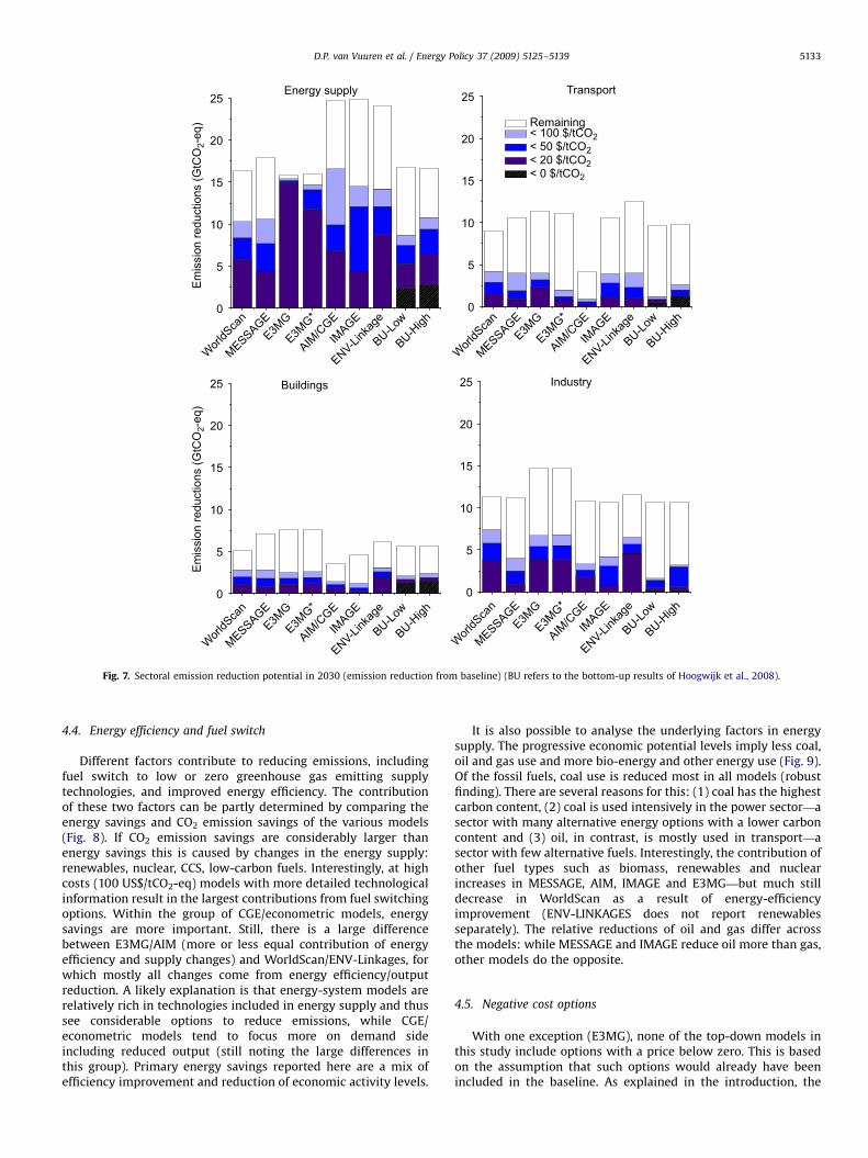
Fig. 7 shows the emission mitigation potentials per sector(total greenhouse gas emissions; reporting emission reductions atthe point of emission, i.e. emission reductions due to electricitysavings in end-use sectors are reported as part of the potential forthe energy supply sector). We present the emission reductionpotentials at different cost levels and the remaining emissions,allowing an assessment of both the absolute emission reductionsacross different sectors and the relative reduction compared tobaseline across the models and sectors. This is consistent with ourearlier conclusion that emission reductions have to be interpretedin the context of baseline emissions. Below, we discuss themitigation potentials by sector—and indicate some of theunderlying reasons for differences. Overall, the results indicatethat differences originate from specific model settings rather thanmodel structure, as, for instance, illustrated by the fact that formost sectors results differ among the three CGE models in asimilar way as between the bottom-up and top-down models.

The figure shows that in terms of emission reduction theenergy supply sector has the largest mitigation potential in theorder of 14 GtCO2-eq. This includes the indirect effects of reducedelectricity use in end-use sectors. The reductions originate from(1) improved efficiency in end-use, (2) demand reduction due tohigher electricity prices and (3) using different technologies in thepower sector: substitution of coal by natural gas and fossil-fuel-based technologies by biomass, renewable energy sources and/orfossil-fuel-based technologies in combination with carbon-cap-ture-and-storage (CCS). Compared to the baseline, the top-downmodels indicate that a substantial share of emissions, around 75%(65–90%), can be reduced at carbon prices below 100$/tCO2. Thebottom-up analysis reports a smaller potential: 50–65%. Also the

bottom-up analysis indicates the energy supply sector to have thelargest potential in both absolute and relative terms, but thepotential is lower than that of several top-down models. The top-down potential in the energy supply sector (mostly power sector)could be relatively large as the models have considerabletechnology detail for this sector and sector implementationbarriers are relatively low. Both factors are likely to lead to a highreduction potential in top-down models. The more limitedpotential in bottom-up studies is reportedly due to considerationof rate at which new capital is introduced in each sector(Hoogwijk et al., 2008), but this is also accounted for in severalof the top-down models. More attention to underlying factorswould be needed to explain the difference including for instanceassumed technical life-times or capital depreciation.

The mitigation potential in the transport sector is limitedcompared to other sectors (20–40% in the top-down models;15–25% in the bottom-up analysis)—which is consistent withearlier findings (Fisher et al., 2007; van Vuuren et al., 2007). Thelimitation in transport emission reductions comes from a limitedresponse to an increase in primary energy prices (as final energyprices are strongly determined by taxes), and the fact thatalternative technologies are still expensive or have other dis-advantages e.g. limited range and limitation in bio-energy supply(covered explicitly in those models that include technologydetail). Important R&D breakthroughs are still needed in thissector, e.g. with respect to fuel cells and batteries or conversion ofsecond generation biofuels. The oil price forms a major un-certainty in the transport sector (as variations in the oil price canbe of similar magnitude as the carbon taxes that are considered).Obviously, the number of technologies considered in the transportsector (biofuels, electric/hydrogen-based transport) and the costdevelopment of these technologies have a major impact onthe results for those models that include technology detail. Therelatively low potential in the bottom-up study compared to thetop-down studies is at least partly caused by the fact thatreduction measures were not considered for the completesector—but for passenger transport only. Moreover, modal shiftand behavioral change have not been included in the bottom-upstudy, while these are implicitly or explicitly included in some ofthe top-down models.

In the buildings sector, both the top-down models and thebottom-up study show a reduction potential of around 40% atcosts below 100$/tCO2. In the bottom-up analysis, the far majorityof options in this sector is also available at costs below20$/tCO2—but this is not seen in the (top-down) model results.AR4 reports a much larger potential for the buildings sector(Barker et al., 2007). An important factor explaining the differenceis that we have assigned the reductions in electricity use to theenergy supply sector (point of emission) while the IPCC reportedthem for the buildings sector (point of action). Secondly, Hoogwijket al. (2008) revised the potential in the buildings sectordownward based on a reappraisal of the existing literature.

Finally, the top-down and bottom-up results differ strongly forthe industrial sector. Here, the bottom-up results (15–30%reduction at costs below 100$/tCO2) are much lower than themodel results (35–60%). For the top-down models, results in thissector differ more between the models than in other sectors. TheMESSAGE model’s low potential is explained by a relatively highbaseline efficiency (given a rapid expansion in this sector; thus aconsiderable amount of new capital). The potential of the bottom-up study is constrained by several factors. Consistent with IPCC,the bottom-up study only considered currently best-availabletechnology as means to reduce emissions (Hoogwijk et al., 2009).Second, bottom-up analysts included stock turn-over (as do someof the top-down models). Finally, the bottom-up assessment doesnot include a reduction in production levels as a reduction option.

Page 9

ARTICLE IN PRESS

WorldS

can

MESSAGEE3M

G

E3MG*

AIM/C

GE

IMAGE

ENV-Link

age

BU-Low

BU-High

WorldS

can

MESSAGEE3M

G

E3MG*

AIM/C

GE

IMAGE

ENV-Link

age

BU-Low

BU-High

WorldS

can

MESSAGEE3M

G

E3MG*

AIM/C

GE

IMAGE

ENV-Link

age

BU-Low

BU-High

WorldS

can

MESSAGEE3M

G

E3MG*

AIM/C

GE

IMAGE

ENV-Link

age

BU-Low

BU-High

0

5

10

15

20

25

Em

issi

on re

duct

ions

(GtC

O2-

eq)

0

5

10

15

20

25

Remaining < 100 $/tCO2 < 50 $/tCO2 < 20 $/tCO2 < 0 $/tCO2

0

5

10

15

20

25 Industry

Transport

Buildings

Em

issi

on re

duct

ions

(GtC

O2-

eq)

Energy supply

0

5

10

15

20

25

Fig. 7. Sectoral emission reduction potential in 2030 (emission reduction from baseline) (BU refers to the bottom-up results of Hoogwijk et al., 2008).

D.P. van Vuuren et al. / Energy Policy 37 (2009) 5125–5139 5133

4.4. Energy efficiency and fuel switch

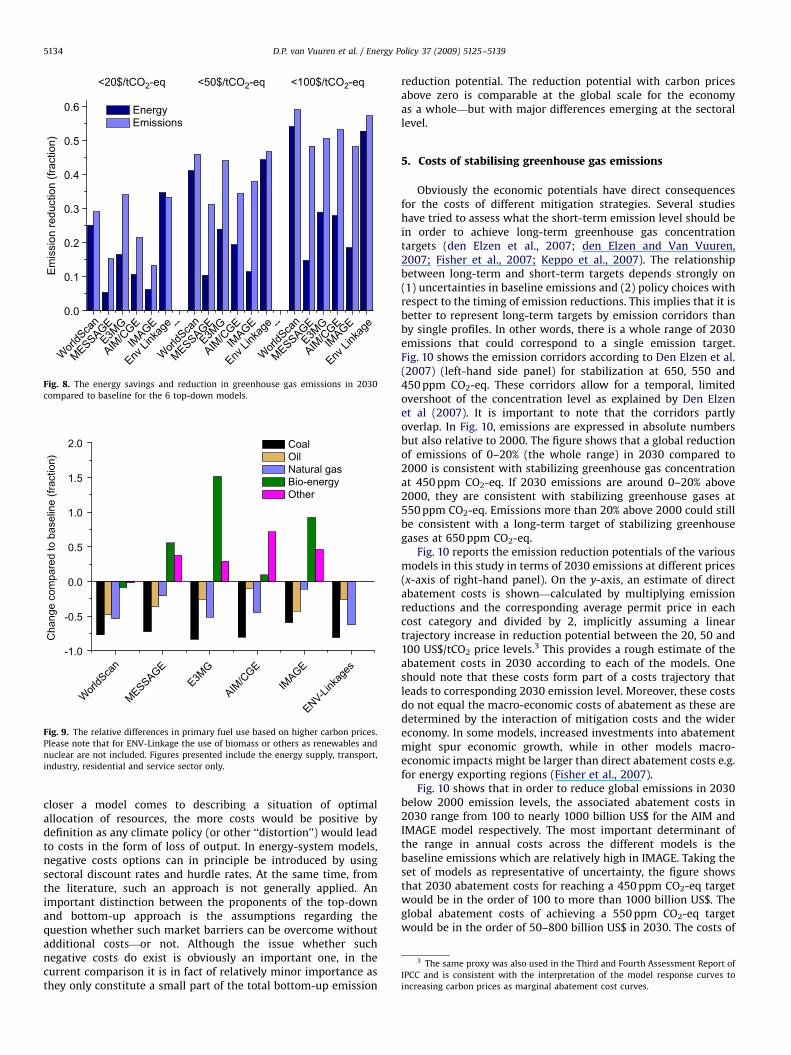
Different factors contribute to reducing emissions, includingfuel switch to low or zero greenhouse gas emitting supplytechnologies, and improved energy efficiency. The contributionof these two factors can be partly determined by comparing theenergy savings and CO2 emission savings of the various models(Fig. 8). If CO2 emission savings are considerably larger thanenergy savings this is caused by changes in the energy supply:renewables, nuclear, CCS, low-carbon fuels. Interestingly, at highcosts (100 US$/tCO2-eq) models with more detailed technologicalinformation result in the largest contributions from fuel switchingoptions. Within the group of CGE/econometric models, energysavings are more important. Still, there is a large differencebetween E3MG/AIM (more or less equal contribution of energyefficiency and supply changes) and WorldScan/ENV-Linkages, forwhich mostly all changes come from energy efficiency/outputreduction. A likely explanation is that energy-system models arerelatively rich in technologies included in energy supply and thussee considerable options to reduce emissions, while CGE/econometric models tend to focus more on demand sideincluding reduced output (still noting the large differences inthis group). Primary energy savings reported here are a mix ofefficiency improvement and reduction of economic activity levels.

It is also possible to analyse the underlying factors in energysupply. The progressive economic potential levels imply less coal,oil and gas use and more bio-energy and other energy use (Fig. 9).Of the fossil fuels, coal use is reduced most in all models (robustfinding). There are several reasons for this: (1) coal has the highestcarbon content, (2) coal is used intensively in the power sector—asector with many alternative energy options with a lower carboncontent and (3) oil, in contrast, is mostly used in transport—asector with few alternative fuels. Interestingly, the contribution ofother fuel types such as biomass, renewables and nuclearincreases in MESSAGE, AIM, IMAGE and E3MG—but much stilldecrease in WorldScan as a result of energy-efficiencyimprovement (ENV-LINKAGES does not report renewablesseparately). The relative reductions of oil and gas differ acrossthe models: while MESSAGE and IMAGE reduce oil more than gas,other models do the opposite.

4.5. Negative cost options

With one exception (E3MG), none of the top-down models inthis study include options with a price below zero. This is basedon the assumption that such options would already have beenincluded in the baseline. As explained in the introduction, the

Page 10

ARTICLE IN PRESS

WorldS

can

MESSAGEE3M

G

AIM/C

GE

IMAGE

Env Li

nkag

e --

WorldS

can

MESSAGEE3M

G

AIM/C

GE

IMAGE

Env Li

nkag

e --

WorldS

can

MESSAGEE3M

G

AIM/C

GE

IMAGE

Env Li

nkag

e0.0

0.1

0.2

0.3

0.4

0.5

0.6

<100$/tCO2-eq<50$/tCO2-eq

Em

issi

on re

duct

ion

(frac

tion)

Energy Emissions

<20$/tCO2-eq

Fig. 8. The energy savings and reduction in greenhouse gas emissions in 2030

compared to baseline for the 6 top-down models.

WorldS

can

MESSAGEE3M

G

AIM/C

GE

IMAGE

ENV-Link

ages

-1.0

-0.5

0.0

0.5

1.0

1.5

2.0

Cha

nge

com

pare

d to

bas

elin

e (fr

actio

n)

Coal Oil Natural gas Bio-energy Other

Fig. 9. The relative differences in primary fuel use based on higher carbon prices.

Please note that for ENV-Linkage the use of biomass or others as renewables and

nuclear are not included. Figures presented include the energy supply, transport,

industry, residential and service sector only.

3 The same proxy was also used in the Third and Fourth Assessment Report of

IPCC and is consistent with the interpretation of the model response curves to

increasing carbon prices as marginal abatement cost curves.

D.P. van Vuuren et al. / Energy Policy 37 (2009) 5125–51395134

closer a model comes to describing a situation of optimalallocation of resources, the more costs would be positive bydefinition as any climate policy (or other ‘‘distortion’’) would leadto costs in the form of loss of output. In energy-system models,negative costs options can in principle be introduced by usingsectoral discount rates and hurdle rates. At the same time, fromthe literature, such an approach is not generally applied. Animportant distinction between the proponents of the top-downand bottom-up approach is the assumptions regarding thequestion whether such market barriers can be overcome withoutadditional costs—or not. Although the issue whether suchnegative costs do exist is obviously an important one, in thecurrent comparison it is in fact of relatively minor importance asthey only constitute a small part of the total bottom-up emission

reduction potential. The reduction potential with carbon pricesabove zero is comparable at the global scale for the economyas a whole—but with major differences emerging at the sectorallevel.

5. Costs of stabilising greenhouse gas emissions

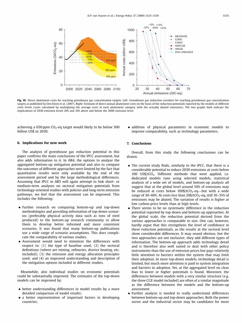
Obviously the economic potentials have direct consequencesfor the costs of different mitigation strategies. Several studieshave tried to assess what the short-term emission level should bein order to achieve long-term greenhouse gas concentrationtargets (den Elzen et al., 2007; den Elzen and Van Vuuren,2007; Fisher et al., 2007; Keppo et al., 2007). The relationshipbetween long-term and short-term targets depends strongly on(1) uncertainties in baseline emissions and (2) policy choices withrespect to the timing of emission reductions. This implies that it isbetter to represent long-term targets by emission corridors thanby single profiles. In other words, there is a whole range of 2030emissions that could correspond to a single emission target.Fig. 10 shows the emission corridors according to Den Elzen et al.(2007) (left-hand side panel) for stabilization at 650, 550 and450 ppm CO2-eq. These corridors allow for a temporal, limitedovershoot of the concentration level as explained by Den Elzenet al (2007). It is important to note that the corridors partlyoverlap. In Fig. 10, emissions are expressed in absolute numbersbut also relative to 2000. The figure shows that a global reductionof emissions of 0–20% (the whole range) in 2030 compared to2000 is consistent with stabilizing greenhouse gas concentrationat 450 ppm CO2-eq. If 2030 emissions are around 0–20% above2000, they are consistent with stabilizing greenhouse gases at550 ppm CO2-eq. Emissions more than 20% above 2000 could stillbe consistent with a long-term target of stabilizing greenhousegases at 650 ppm CO2-eq.

Fig. 10 reports the emission reduction potentials of the variousmodels in this study in terms of 2030 emissions at different prices(x-axis of right-hand panel). On the y-axis, an estimate of directabatement costs is shown—calculated by multiplying emissionreductions and the corresponding average permit price in eachcost category and divided by 2, implicitly assuming a lineartrajectory increase in reduction potential between the 20, 50 and100 US$/tCO2 price levels.3 This provides a rough estimate of theabatement costs in 2030 according to each of the models. Oneshould note that these costs form part of a costs trajectory thatleads to corresponding 2030 emission level. Moreover, these costsdo not equal the macro-economic costs of abatement as these aredetermined by the interaction of mitigation costs and the widereconomy. In some models, increased investments into abatementmight spur economic growth, while in other models macro-economic impacts might be larger than direct abatement costs e.g.for energy exporting regions (Fisher et al., 2007).

Fig. 10 shows that in order to reduce global emissions in 2030below 2000 emission levels, the associated abatement costs in2030 range from 100 to nearly 1000 billion US$ for the AIM andIMAGE model respectively. The most important determinant ofthe range in annual costs across the different models is thebaseline emissions which are relatively high in IMAGE. Taking theset of models as representative of uncertainty, the figure showsthat 2030 abatement costs for reaching a 450 ppm CO2-eq targetwould be in the order of 100 to more than 1000 billion US$. Theglobal abatement costs of achieving a 550 ppm CO2-eq targetwould be in the order of 50–800 billion US$ in 2030. The costs of

Page 11

ARTICLE IN PRESS

200

200

400

600

800

1000+20%

+10%

Ann

ual c

osts

(bill

ion

US

$)

-20%-10%

Annual emissions (GtC-eq)

MESSAGE E3MG E3MG* AIM/CGE IMAGE ENV-LINKAGES

2000

20000

20

40

60

80

+20%+10%

-20%

2000

450 ppm

550 ppm

Em

issi

ons

(GtC

O2-

eq)

650 ppm-10%

2020 2040 2060 2080 2100 30 40 50 60 70

Fig. 10. Direct abatement costs for reaching greenhouse gas concentration targets. Left: Greenhouse gas reduction corridors for reaching greenhouse gas concentration

targets as published by Den Elzen et al. (2007). Right: Estimate of direct annual abatement costs on the basis of the reduction potentials reported by the models at different

costs levels (costs calculated by multiplying the average costs in each abatement category with the actually abated emissions). The two graphs both indicate the

implications of 2030 emission levels 20% and 10% above and below the 2000 emission level.

D.P. van Vuuren et al. / Energy Policy 37 (2009) 5125–5139 5135

achieving a 650 ppm CO2-eq target would likely to be below 300billion US$ in 2030.

6. Implications for new work

The analysis of greenhouse gas reduction potential in thispaper confirms the main conclusions of the IPCC assessment, butalso adds information to it. In AR4, the options to analyse theaggregated bottom-up mitigation potential and also to comparethe outcomes of different approaches were limited by the fact thatquantitative results were only available by the end of theassessment period and by the large methodological differences.Assuming that IPCC in AR5 will again attempt to link short- ormedium-term analyses on sectoral mitigation potentials fromtechnology-oriented studies with policies and long-term emissionpathways, we feel that the assessment can be improved. Thisincludes the following:

�

Further research on comparing bottom-up and top-downmethodologies and providing information of top-down scenar-ios (preferably physical activity data such as tons of steelproduced) to the bottom-up research community to allowthem to develop better informed and more consistentscenarios. It was found that many bottom-up publicationsuse a wide range of scenario assumptions. This does compli-cate the comparability of various studies. � Assessment would need to minimize the differences with

respect to: (1) the type of baseline used; (2) the sectoraldefinitions (where are mining, refineries, district heating, etc.included); (3) the emission and energy allocation principlesused; and (4) an improved understanding and description ofthe mitigation options included in different studies.

Meanwhile, also individual studies on economic potentialscould be substantially improved. The estimates of the top-downmodels can be improved by:

�

better understanding differences in model results by a moredetailed comparison of model results; � a better representation of important factors in developing

countries;

�

addition of physical parameters in economic models toimprove comparability, such as technology parameters.

7. Conclusions

Overall, from this study the following conclusions can bedrawn:

�

The current study finds, similarly to the IPCC, that there is aconsiderable potential to reduce 2030 emissions at costs below100 US$/tCO2. Different methods that were applied, i.e.dedicated models runs using selected models, statisticalanalysis of a wide set of models, and bottom-up analysis allsuggest that at the global level around 50% of emissions maybe reduced at costs below 100$/tCO2-eq—but with a widerange of 30–60%. At costs less than 20$/tCO2-eq, still 10–35% ofemissions may be abated. The variation of results is higher atlow carbon-price levels than at high levels. � There seems to be no systematic difference in the reduction

potential reported by top-down and bottom-up approaches. Atthe global scale, the reduction potential derived from thevarious approaches is comparable in size. One can, however,hardly argue that this strengthens the level of confidence inthese reduction potentials, as the results at the sectoral levelshow considerable differences. It may sound obvious, but thetwo approaches are not exclusive; they add different types ofinformation. The bottom-up approach adds technology detailand is therefore also well suited to deal with other policyinstruments than the use of emission prices but pays relativelylittle attention to barriers within the system that may limittheir adoption. In most top-down models, technology detail islimited, but much more attention is paid to system integrationand barriers to adoption. Yet, at the aggregated level no clearbias to lower or higher potentials is found. Moreover, thedifferences between models with a very similar structure (e.g.the three CGE model included) are often of a similar magnitudeas the difference between the models and the bottom-upassessment.

� Further analysis is needed to really understand differences

between bottom-up and top-down approaches. Both the powersector and the industrial sector may be candidates for more

Page 12

ARTICLE IN PRESS

TabOve

Typ

Ma

Stru

Mo

Clim

(su

Clim

(de

D.P. van Vuuren et al. / Energy Policy 37 (2009) 5125–51395136

in-depth analysis, given the surprisingly large differences butalso degree of detail that top-down models and bottom-upapproaches include for these sectors.

� The largest reduction potential as a response to carbon prices

exists in the energy supply sector. The energy supply sectormakes up more than a third of the total potential in mostmodels. However, it should be noted that in this study we alsoreport electricity savings under this sector as we use theconvention to report emissions where they are emitted. Thetransport sector has the lowest relative potential of the sectorscovered in this study. There are considerable uncertainties inthe potentials reported. Important uncertainties include:(1) the potential in non-OECD regions, (2) the buildings sector(wide range of results) and the potential at lower carbon costs(idem).

� Given the differences across model results and existing

uncertainties in factors such as technology development,baseline emissions and macro-economic links, users shouldpreferably consider ranges reported in the literature/assess-ments instead of relying on single models for policy decisions.The uncertainties and the differences in model outcomespartly reflect real intrinsic uncertainties regarding thefuture—and partly reflect more methodological issues (modeltradition, lack of data). There is, however, not one bestapproach or result. Given the ranges that are noted, whichcan easily encompass a 10 %-points in reduction potential, it isconcluded that for decision-making it is preferable to useresults from model comparison studies (such as EMF) orassessments than to use single model results. While using such

le A.1rview of the models used in this study.

WorldScan MESSAGE-MACRO E3MG

e Recursive dynamic

computable

general

equilibrium model

Energy system

model linked to a

computable

general

equilibrium model

Macro-

econometric non

equilibrium hyb

simulation mod

in applications Analysis of

European/world

climate policy

scenarios

Long-term energy/

emission scenarios

Global economic

analysis; short,

medium- and lo

run climate

mitigation

cture Nested CES

production

function

Representation of

energy services and

individual

technologies

Demand-driven

model with an

input-output

structure and

econometrically

estimated

coefficients

del solution Simultaneous

solution of a

system of market-

clearance, zero-

profit and budget-

constraint

conditions

Optimisation of

energy system

costs

Simulation (top-

down module) a

market share

attribution for

energy options

(bottom-up

module)

ate policy

pply)

Represented by

imposed elasticity

of substitution

between capital,

labour, and energy

in a CES production

function

Represented by

choosing different

technologies in

response to price

changes

Supply side:

energy-technolo

submodel

simulating price

effects on

technology

substitution.

ate policy

mand)

Represented by

substitution

processes (capital,

labour and energy)

in CES function

Demand side:

formal co-

integration

econometric

techniques

results, it is important to make results consistent as far aspossible by avoiding different reporting practices, sectoraldefinitions and baselines.

� The economic potentials can be used to make estimates

on annual abatement costs in order to achieve certainstabilization levels. Although uncertainties are considerable,the results of this study suggest that typical marginalabatement costs in 2030 associated with stabilization at 450,550 and 650 ppm CO2-eq would, respectively, be in the order ofless than 0–20$/tCO2-eq, 10–50$/tCO2-eq and around (orabove) 100 US$/tCO2-eq.

Acknowledgements

This study has been performed within the frameworkof the Netherlands Research Programme on Scientific Assess-ment and Policy Analysis for Climate Change (WAB). Wewould like to thank Patrick Todd, Kees Vijverberg (both VROM)and Leo Meyer (PBL) for their valuable input during thisproject. We also thank the anonymous reviewer for his helpfulcomments.

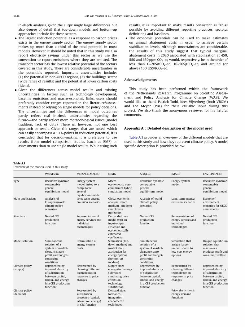
Appendix A. : Detailed description of the model used

Table A.1 provides an overview of the different models that areused in this study and how they represent climate policy. A modelspecific description is provided below.

AIM/CGE IMAGE ENV-LINKAGES

-

rid

el

Recursive dynamic

computable

general

equilibrium model

Energy system

model

Recursive dynamic

computable

general

equilibrium model

ng-

Analysis of world

climate policy

scenarios

Long-term energy/

emission scenarios

Economy/

environment

scenarios for OECD

assessments

Nested CES

production

function

Representation of

energy services and

individual

technologies

Nested CES

production

function

nd

Simultaneous

solution of a

system of market-

clearance, zero-

profit and budget-

constraint

conditions.

Simulation that

assigns larger

market shares to

low-cost energy

options

Unique equilibrium

solution that

maximizes

producer profit and

consumer welfare

gy

Represented by

imposed elasticity

of substitution

between capital,

labour, and energy

in a CES production

function

Represented by

choosing different

technologies in

response to price

changes

Represented by

imposed elasticity

of substitution

between capital,

labour, and energy

in a CES production

functionPrice elasticities in

energy demand

functions

Page 13

ARTICLE IN PRESS

Table A.1 (continued )

WorldScan MESSAGE-MACRO E3MG AIM/CGE IMAGE ENV-LINKAGES

Revenues of carbon

tax

Recycled lump-

sum

Not considered Reduction of

indirect taxes and

investments to

stimulate low-

carbon production

methods

Recycled lump-

sum to household

sector

Not considered Recycled lump-

sum

Inertia No delay Vintage structure

with the possibility

of premature face

out

Different responses

are assigned per

type of capital/

technology

Specific lifetimes

per economic

sector (vintage

structure)

Old/new capital

vintage (with

slower response in

old capital

functions)

Sectors 18 production

sectors (5 energy

sectors)

7 end-use sectors

coupled to a

technology-rich

supply sector

42 economic

sectors

20 production

sectors and 12

power sectors

5 end-use sectors

and 6 energy

supply sectors

17 economic

sectors (5 energy

sectors)

Energy carriers Production sectors:

oil, coal, gas, oil/

coal products,

electricity

Primary carriers:

coal, oil, natural

gas, bio-energy,

wind, solar, hydro,

geothermal.

Various secondary

energy carriers

including

electricity heat,

hydrogen, coal/gas

liquids, etc.

12 energy carriers Primary carriers:

coal, oil, natural

gas, bio-energy,

wind, solar, hydro,

geothermal and

nuclear.

Primary carriers:

coal, oil, natural

gas, bio-energy,

wind, solar, hydro

Final energy

carriers: solid,

liquid and gas,

electrilcity, and

biomass

(traditional).

Greenhouse gases CO2 All GHGs Focus on CO2 All GHGs All GHGs All GHGs

D.P. van Vuuren et al. / Energy Policy 37 (2009) 5125–5139 5137

A.1. WorldScan

WorldScan model is a computable general-equilibrium model,based on a set of nested CES production functions (Lejour et al.,2006). The model is mainly used for analysis of European andworld climate policies. The model has 18 production sectors thatuse energy as intermediate input, plus final consumption ofprivate households. Of the 18 sectors, 5 are energy sectors: oil,coal, gas, processed oil and coal products, electricity. The nestedCES production functions are defined at the level of the sectors inNational Accounts.

Energy efficiency for the reference scenario is based onautonomous energy efficiency improvements. For the policysimulations, energy efficiency improvements and technologyshifts are represented as substitution processes in the sectoralCES production functions.

A.2. MESSAGE

MESSAGE is a systems engineering optimization model usedfor medium- to long-term energy-system planning, energy policyanalysis, and scenario development (Messner and Strubegger,1995; Riahi et al., 2007). The model provides a framework forrepresenting an energy system with all its interdependenciesacross 11 macro-regions. Scenarios are developed by MESSAGEthrough minimizing the total systems costs under the constraintsimposed on the energy system. Given this information and otherscenario features such as the demand for energy services, themodel configures the evolution of the energy system from thebase year to the end of the time horizon (in 10 year steps). Itprovides the installed capacities of technologies, energy outputsand inputs, energy requirements at various stages of the energysystems, costs, emissions, etc.

MESSAGE model is linked to the MACRO model to includemacro-economic impact of policies on energy demand. The link isestablished by using MESSAGE results on total and marginal costs

of energy supply to derive the quadratic demand functions forMACRO. MACRO defines an inter-temporal utility function of asingle representative producer–consumer in each of the model’sworld regions, which is maximized. The main variables of thismodule are the production factors capital stock, available labor,and energy inputs, which together determine the total output ofan economy according to a nested constant elasticity of substitu-tion (CES) production function. The optimal quantities of theproduction factors are determined by their relative prices. Energydemand curves are given in two categories, electric and non-electric energy, as quadratic functions of energy prices.

A.3. E3MG

Energy–Environment–Economy Modelling at the Global level(E3MG) is a macro-econometric non-equilibrium hybrid simula-tion model of the global E3 system, estimated on annual data1970–2002 and projecting annually to 2020 and every 10 years to2100 (Barker et al., 2006; Barker and Scrieciu, 2009; Barker et al.,2008). The model is based upon a Post-Keynesian economic viewof the long-run, adopting a ‘‘history’’ approach of cumulativecausation and demand-led growth, and incorporating technologi-cal progress in gross investment enhanced by R&D expenditures.E3MG is highly disaggregated, with 20 world regions, 42 sectors,19 fuel users (amongst which 12 primary and 7 final energy users)and 12 energy carriers. Energy-efficiency improvements and shiftsto a low-carbon technology are represented via both formal co-integration econometric techniques that identify long-run macro-trends of the global energy-economy system, as well bottom-upenergy-technology simulations allowing for the explicit modellingof 28 energy technologies (7 carbon-intensive and 21 low-carbontechnologies). Climate policy is implemented via full auctioning ofcarbon permits to energy-related sectors and carbon taxation forrest of the sectors, with the revenues raised being recycled tomaintain fiscal neutrality (via reduction in indirect taxes) and(in some cases) to further stimulate low-carbon production

Page 14

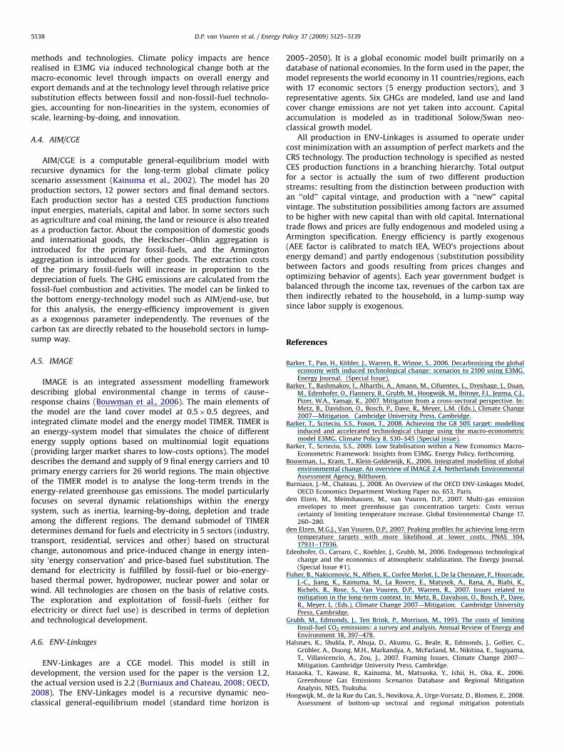
ARTICLE IN PRESS

D.P. van Vuuren et al. / Energy Policy 37 (2009) 5125–51395138

methods and technologies. Climate policy impacts are hencerealised in E3MG via induced technological change both at themacro-economic level through impacts on overall energy andexport demands and at the technology level through relative pricesubstitution effects between fossil and non-fossil-fuel technolo-gies, accounting for non-linearities in the system, economies ofscale, learning-by-doing, and innovation.

A.4. AIM/CGE

AIM/CGE is a computable general-equilibrium model withrecursive dynamics for the long-term global climate policyscenario assessment (Kainuma et al., 2002). The model has 20production sectors, 12 power sectors and final demand sectors.Each production sector has a nested CES production functionsinput energies, materials, capital and labor. In some sectors suchas agriculture and coal mining, the land or resource is also treatedas a production factor. About the composition of domestic goodsand international goods, the Heckscher–Ohlin aggregation isintroduced for the primary fossil-fuels, and the Armingtonaggregation is introduced for other goods. The extraction costsof the primary fossil-fuels will increase in proportion to thedepreciation of fuels. The GHG emissions are calculated from thefossil-fuel combustion and activities. The model can be linked tothe bottom energy-technology model such as AIM/end-use, butfor this analysis, the energy-efficiency improvement is givenas a exogenous parameter independently. The revenues of thecarbon tax are directly rebated to the household sectors in lump-sump way.

A.5. IMAGE

IMAGE is an integrated assessment modelling frameworkdescribing global environmental change in terms of cause–response chains (Bouwman et al., 2006). The main elements ofthe model are the land cover model at 0.5�0.5 degrees, andintegrated climate model and the energy model TIMER. TIMER isan energy-system model that simulates the choice of differentenergy supply options based on multinomial logit equations(providing larger market shares to low-costs options). The modeldescribes the demand and supply of 9 final energy carriers and 10primary energy carriers for 26 world regions. The main objectiveof the TIMER model is to analyse the long-term trends in theenergy-related greenhouse gas emissions. The model particularlyfocuses on several dynamic relationships within the energysystem, such as inertia, learning-by-doing, depletion and tradeamong the different regions. The demand submodel of TIMERdetermines demand for fuels and electricity in 5 sectors (industry,transport, residential, services and other) based on structuralchange, autonomous and price-induced change in energy inten-sity ‘energy conservation’ and price-based fuel substitution. Thedemand for electricity is fulfilled by fossil-fuel or bio-energy-based thermal power, hydropower, nuclear power and solar orwind. All technologies are chosen on the basis of relative costs.The exploration and exploitation of fossil-fuels (either forelectricity or direct fuel use) is described in terms of depletionand technological development.

A.6. ENV-Linkages

ENV-Linkages are a CGE model. This model is still indevelopment, the version used for the paper is the version 1.2,the actual version used is 2.2 (Burniaux and Chateau, 2008; OECD,2008). The ENV-Linkages model is a recursive dynamic neo-classical general-equilibrium model (standard time horizon is

2005–2050). It is a global economic model built primarily on adatabase of national economies. In the form used in the paper, themodel represents the world economy in 11 countries/regions, eachwith 17 economic sectors (5 energy production sectors), and 3representative agents. Six GHGs are modeled, land use and landcover change emissions are not yet taken into account. Capitalaccumulation is modeled as in traditional Solow/Swan neo-classical growth model.

All production in ENV-Linkages is assumed to operate undercost minimization with an assumption of perfect markets and theCRS technology. The production technology is specified as nestedCES production functions in a branching hierarchy. Total outputfor a sector is actually the sum of two different productionstreams: resulting from the distinction between production withan ‘‘old’’ capital vintage, and production with a ‘‘new’’ capitalvintage. The substitution possibilities among factors are assumedto be higher with new capital than with old capital. Internationaltrade flows and prices are fully endogenous and modeled using aArmington specification. Energy efficiency is partly exogenous(AEE factor is calibrated to match IEA, WEO’s projections aboutenergy demand) and partly endogenous (substitution possibilitybetween factors and goods resulting from prices changes andoptimizing behavior of agents). Each year government budget isbalanced through the income tax, revenues of the carbon tax arethen indirectly rebated to the household, in a lump-sump waysince labor supply is exogenous.

References

Barker, T., Pan, H., Kohler, J., Warren, R., Winne, S., 2006. Decarbonizing the globaleconomy with induced technological change: scenarios to 2100 using E3MG.Energy Journal. (Special Issue).

Barker, T., Bashmakov, I., Alharthi, A., Amann, M., Cifuentes, L., Drexhage, J., Duan,M., Edenhofer, O., Flannery, B., Grubb, M., Hoogwijk, M., Ibitoye, F.I., Jepma, C.J.,Pizer, W.A., Yamaji, K., 2007. Mitigation from a cross-sectoral perspective. In:Metz, B., Davidson, O., Bosch, P., Dave, R., Meyer, L.M. (Eds.), Climate Change2007—Mitigation. Cambridge University Press, Cambridge.

Barker, T., Scrieciu, S.S., Foxon, T., 2008. Achieving the G8 50% target: modellinginduced and accelerated technological change using the macro-econometricmodel E3MG. Climate Policy 8, S30–S45 (Special issue).

Barker, T., Scrieciu, S.S., 2009. Low Stabilisation within a New Economics Macro-Econometric Framework: Insights from E3MG. Energy Policy, forthcoming.

Bouwman, L., Kram, T., Klein-Goldewijk, K., 2006. Integrated modelling of globalenvironmental change. An overview of IMAGE 2.4. Netherlands EnvironmentalAssessment Agency, Bilthoven.

Burniaux, J.-M., Chateau, J., 2008. An Overview of the OECD ENV-Linkages Model,OECD Economics Department Working Paper no. 653, Paris.

den Elzen, M., Meinshausen, M., van Vuuren, D.P., 2007. Multi-gas emissionenvelopes to meet greenhouse gas concentration targets: Costs versuscertainty of limiting temperature increase. Global Environmental Change 17,260–280.

den Elzen, M.G.J., Van Vuuren, D.P., 2007. Peaking profiles for achieving long-termtemperature targets with more likelihood at lower costs. PNAS 104,17931–17936.

Edenhofer, O., Carraro, C., Koehler, J., Grubb, M., 2006. Endogenous technologicalchange and the economics of atmospheric stabilization. The Energy Journal.(Special Issue #1).

Fisher, B., Nakicenovic, N., Alfsen, K., Corfee Morlot, J., De la Chesnaye, F., Hourcade,J.-C., Jiang, K., Kainuma, M., La Rovere, E., Matysek, A., Rana, A., Riahi, K.,Richels, R., Rose, S., Van Vuuren, D.P., Warren, R., 2007. Issues related tomitigation in the long-term context. In: Metz, B., Davidson, O., Bosch, P., Dave,R., Meyer, L. (Eds.), Climate Change 2007—Mitigation. Cambridge UniversityPress, Cambridge.

Grubb, M., Edmonds, J., Ten Brink, P., Morrison, M., 1993. The costs of limitingfossil-fuel CO2 emissions: a survey and analysis. Annual Review of Energy andEnvironment 18, 397–478.

Halsnæs, K., Shukla, P., Ahuja, D., Akumu, G., Beale, R., Edmonds, J., Gollier, C.,Grubler, A., Duong, M.H., Markandya, A., McFarland, M., Nikitina, E., Sugiyama,T., Villavicencio, A., Zou, J., 2007. Framing Issues, Climate Change 2007—

Mitigation. Cambridge University Press, Cambridge.Hanaoka, T., Kawase, R., Kainuma, M., Matsuoka, Y., Ishii, H., Oka, K., 2006.

Greenhouse Gas Emissions Scenarios Database and Regional MitigationAnalysis. NIES, Tsukuba.

Hoogwijk, M., de la Rue du Can, S., Novikova, A., Urge-Vorsatz, D., Blomen, E., 2008.Assessment of bottom-up sectoral and regional mitigation potentials

Page 15

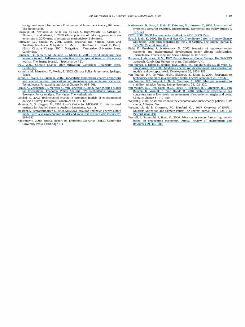
ARTICLE IN PRESS

D.P. van Vuuren et al. / Energy Policy 37 (2009) 5125–5139 5139

background report. Netherlands Environmental Assessment Agency, Bilthoven.The Netherlands.

Hoogwijk, M., Novikova, A., de la Rue du Can, S., Urge-Vorsatz, D., Sathaye, J.,Blomen, E., and Worrell, E., 2009. Global potential of reducing greenhouse gasemissions in 2030 using a bottom-up methodology. Submitted.

Hourcade, J.C., Shukla, P., 2001. Global, Regional and National Costs andAncillary Benefits of Mitigation. In: Metz, B., Davidson, O., Swart, R., Pan, J.(Eds.), Climate Change 2001: Mitigation. Cambridge University Press,Cambridge.

Hourcade, J.C., Jaccard, M., Bataille, C., Ghersi, F., 2006. Hybrid modeling: newanswers to old challenges introduction to the special issue of the energyjournal. The Energy Journal. (Special issue #2).

IPCC, 2007. Climate Change 2007–Mitigation. Cambridge University Press,Cambridge.

Kainuma, M., Matsuoka, Y., Morita, T., 2002. Climate Policy Assessment. Springer,Tokyo.

Keppo, I., O’Neill, B.C., Riahi, K., 2007. Probabilistic temperature change projectionsand energy system implications of greenhouse gas emission scenarios.Technological Forecasting and Social Change 74, 936–961.

Lejour, A., Veenendaal, P., Verweij, G., van Leeuwen, N., 2006. WorldScan: a Modelfor International Economic Policy Analysis. CPB Netherlands Bureau forEconomic Policy Analysis, The Hague, The Netherlands.

Loschel, A., 2002. Technological change in economic models of environmentalpolicy: a survey. Ecological Economics 43, 105–126.

Messner, S., Strubegger, M., 1995. User’s Guide for MESSAGE III. InternationalInstitute for Applied Systems Analysis, Laxenburg, Austria.

Messner, S., Schrattenholzer, L., 2000. MESSAGE-MACRO: linking an energy supplymodel with a macroeconomic model and solving it interactively. Energy 25,267–282.

Nakicenovic, 2000. Special Report on Emissions Scenarios (SRES). CambridgeUniversity Press, Cambridge, UK.

Nakicenovic, N., Kolp, P., Riahi, K., Kainuma, M., Hanaoka, T., 2006. Assessment ofemissions scenarios revisited. Environmental Economics and Policy Studies 7,137–173.

OECD, 2008. OECD Environmental Outlook to 2030. OECD, Paris.Rao, S., Riahi, K., 2006. The Role of Non-CO2 Greenhouse Gases in Climate Change

Mitigation: Long-term Scenarios for the 21st Century. The Energy Journal 1,177–200 (Special Issue #3).

Riahi, K., Gruebler, A., Nakicenovic, N., 2007. Scenarios of long-term socio-economic and environmental development under climate stabilization.Technological Forecasting and Social Change 74, 887–935.

Rotmans, J., de Vries, H.J.M., 1997. Perspectives on Global Change, The TARGETSapproach. Cambridge University press, Cambridge (UK).

van Ruijven, B., Urban, F., Benders, R.M.J., Moll, H.C., van der Sluijs, J.P., de Vries, B.,van Vuuren, D.P., 2008. Modeling energy and development: an evaluation ofmodels and concepts. World Development 36, 2801–2821.

van Vuuren, D.P., de Vries, H.J.M., Eickhout, B., Kram, T., 2004. Responses totechnology and taxes in a simulated world. Energy Economics 26, 579–601.

van Vuuren, D.P., Weyant, J., De la Chesnaye, F., 2006. Multigas scenarios tostabilise radiative forcing. Energy Economics 28, 102–120.

van Vuuren, D.P., Den Elzen, M.G.J., Lucas, P., Eickhout, B.E., Strengers, B.J., VanRuijven, B., Wonink, S., Van Houdt, R., 2007. Stabilizing greenhouse gasconcentrations at low levels: an assessment of reduction strategies and costs.Climatic Change 81, 119–159.

Weyant, J., 2000. An introduction to the economics of climate change policies. PEWcenter, Arlington VA.

Weyant, J.P., de la Chesnaye, F.C., Blanford, G.J., 2007. Overview of EMF21:Multigas Mitigation and Climate Policy. The Energy Journal (pp. 1–32), 1–32(Special issue #3).

Worrell, E., Ramesohl, S., Boyd, G., 2004. Advances in energy forecasting modelsbased on engineering economics. Annual Review of Environment andResources 29, 345–381.