Comparison of the autoregressive and autocovariance prediction results on different stationary time series Wiesław Kosek University of Agriculture in Krakow,

Comparison of the autoregressive and autocovariance prediction results on different stationary time series

Wiesław Kosek

University of Agriculture in Krakow, Poland

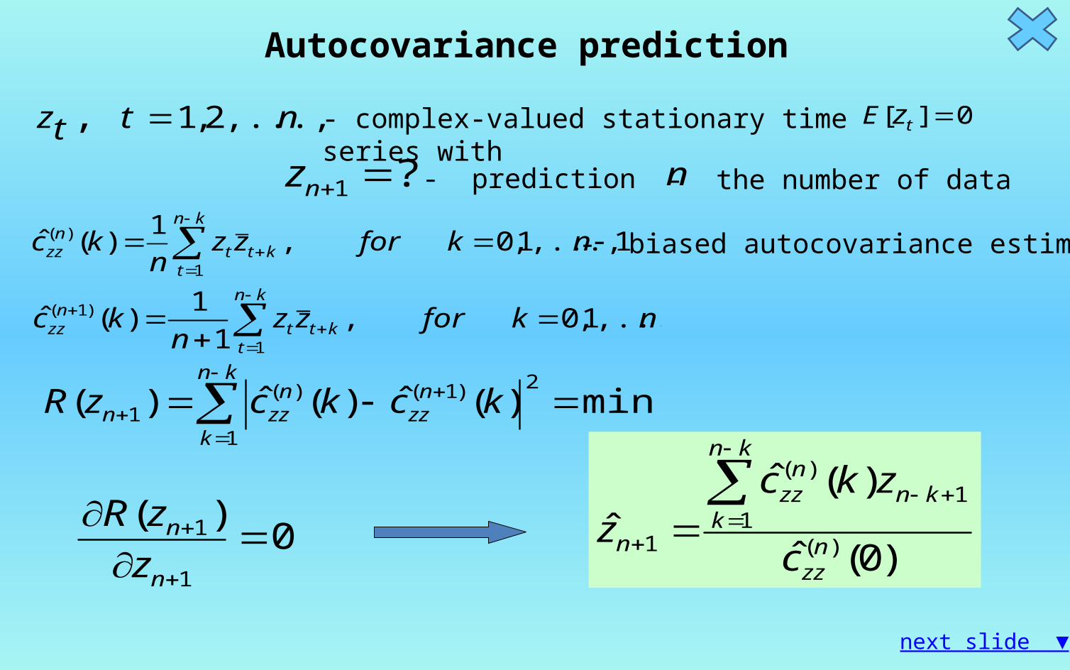
Abstract. The advantages and disadvantages of the autoregressive and autocovariance prediction methods are presented using different model time series similar to the observed geophysical ones, e.g. Earth orientation parameters or sea level anomalies data. In the autocovariance prediction method the first predicted value is determined by the principle that the autocovariances estimated from the extended by the first prediction value series coincide as closely as possible with the autocovariances estimated from the given series. In the autoregressive prediction method the autoregressive model is used to estimate the first prediction value which depends on the autoregressive order and coefficients computed from the autocovariance estimate. In both methods the autocovariance estimations of time series must be computed, thus application of them makes sense when these series are stationary. However, the autoregressive prediction is more suitable for less noisy data and can be applied to short time span series. The autocovariance prediction is recommended for longer time series and but unlike autoregressive method can be applied to more noisy data. The autoregressive method can be applied for time series having close frequency oscillations while the autocovariance prediction is not suitable for such data. In case of the autocovariance prediction the problem of estimation of the appropriate forecast amplitude is also discussed.

1/2European Geosciences Union General Assembly 2015, Vienna | Austria | 12 – 17 April 2015

Autocovariance prediction

Autoregressive prediction

Results

Conclusions

Comparison of the autoregressive and autocovariance prediction results on different stationary time series

Wiesław Kosek

University of Agriculture in Krakow

MODEL DATAt

L

ii

iit nt

T

tAz

1

)(2

exp

iT iA )(ti tn

t

kki nt

1

)(

2/2



Results

Conclusions

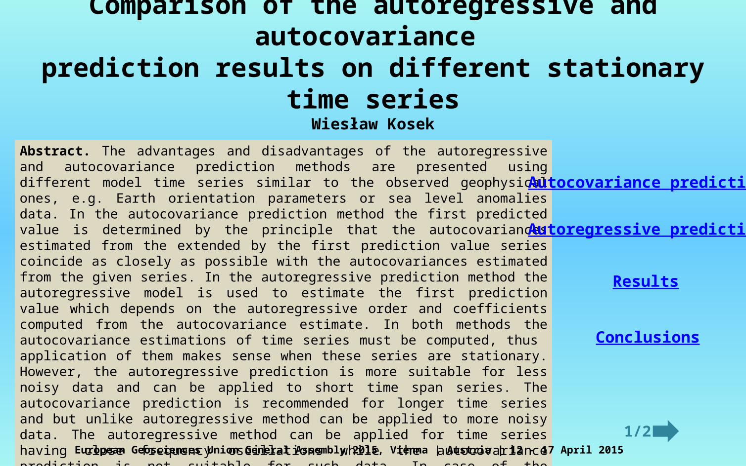
Periods Amplitudes Phases Noise

MODEL 1L=3M=100

20, 30, 50 All equal to 1.0 All equal to 0.0 standard deviations: 0, 3

MODEL 2L=3M=100

50, 57, 60 All equal to 1.0 All equal to 0.0 standard deviations: 0, 1, 2, 3

MODEL 3L=9M=100

10, 15, 20, 25, 40, 60, 90, 120, 180

All equal to 1.0 All equal to 0.0 standard deviations: 0, 1, 2, 3, 5

MODEL 4L=1M=1000

365.24 1.0 Random walk computed by integration of white nose with standard deviations equal to 1o,2o, 3o

standard deviation: 0.1

MODEL 5L=2M=1000

365.24, 182.62 1.0, 0.5 Random walk computed by integration of white nose with standard deviations equal to 2o


MODEL 6L=2M=1000

365.24433.00

0.08, 0.016 Random walk computed by integration of white nose with standard deviations equal to 2o



0)(

1

1

n

n

z

zR

nttz ,...,2,1,

)0(ˆ

)(ˆˆ

)(1

1)(

1 nzz

kn

kkn

nzz

n c

zkcz

1,...,1,0,1

)(ˆ1

)(

nkforzz

nkc

kn

tktt

nzz

nkforzzn

kckn

tktt

nzz ,...,1,0,

1

1)(ˆ

1

)1(

min,)(ˆ)(ˆ)(1

2)1()(1

kn

k

nzz

nzzn kckczR

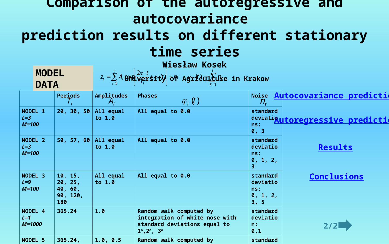
?1 nz

- complex-valued stationary time series with

- prediction

0][ tzE

n - the number of data

- biased autocovariance estimate

next slide ▼

1,...,1,0,)(ˆ)(ˆ)(ˆ)(ˆ1)(ˆ )()()()(

1

)(

nkkckcikckczznkc n

xynyx

nyy

nxxkt

kn

tt

nzz

111 nnn iyxz

1

)(ˆ)()(ˆ 11111111)(

)1(

knyxxyiyyxxkcknkc nknnknnknnkn

nzzn

zz

The biased autocovariances of a complex-valued stationary time series can be expressed by the real-valued auto/cross-covariances of the real and imaginary parts:

After the time series is extended by the first prediction point computed by:

a new estimation of the autocovariance can be computed using the previous one by the following recursion formula:

kn

kknkn

n

k kn

kn

kn

kn

n

n

yx

x

ykb

y

xka

y

x

1

21

21

1

1 1

1

1

1

1

1

)(ˆ)(ˆ )(ˆ)(ˆ)(ˆ )()( kckcka nyy

nxx

)(ˆ)(ˆ)(ˆ )()( kckckb nxy

nyx

where

and it can be used to compute the next prediction point etc. 222 nnn iyxzresults


next slide ▼

tMtMttt nxaxaxax ...2211

Autoregressive order:

Akaike godness-of-fit criterion:

MMon cacacacM ˆˆ...ˆˆˆ)(ˆ 22112

min1

1)()( 2

MN

MNMMP n

MoMM

Mo

Mo

M c

c

c

ccc

ccc

ccc

a

a

a

ˆ

.

ˆ

ˆ

ˆ.ˆˆ

....

ˆ.ˆˆ

ˆ.ˆˆ

ˆ

.

ˆ

ˆ

2

1

1

21

21

11

2

1

Autoregressive coefficients:

11211 ˆ...ˆˆˆ MNMNNN xaxaxax

22112 ˆ...ˆˆˆˆ MNMNtNN xaxaxax

LMNMLNLNLN xaxaxax ...ˆˆˆˆˆ 2211

where

1,...,1,0,1

ˆ1

nkforxx

nc

kn

tkttk

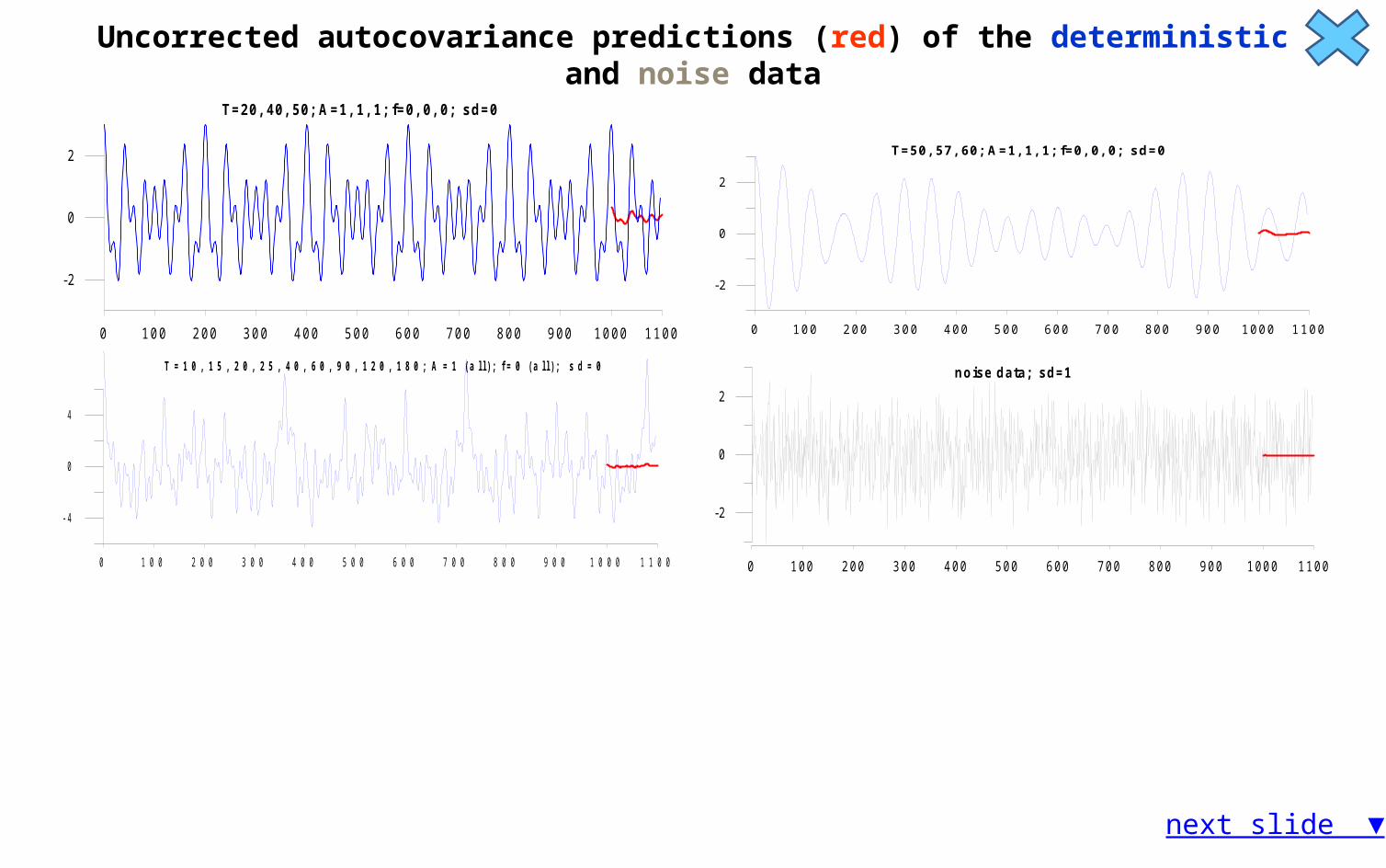
Uncorrected autocovariance predictions (red) of the deterministic and noise data

0 100 200 300 400 500 600 700 800 900 1000 1100

-2

0

2

T=50, 57, 60; A=1, 1, 1; f=0, 0, 0; sd=0

0 100 200 300 400 500 600 700 800 900 1000 1100

-4

0

4

T=10, 15, 20, 25, 40, 60, 90, 120, 180; A=1 (all); f=0 (all); sd=0

0 100 200 300 400 500 600 700 800 900 1000 1100

-2

0

2

T=20, 40, 50; A=1, 1, 1; f=0, 0, 0; sd=0

next slide ▼

0 100 200 300 400 500 600 700 800 900 1000 1100

-2

0

2

noise data; sd=1

Correction to amplitudes of the autocovariance prediction

1. n=0.7×N where N is the total number of data2. computation of the autocovariance ck of xt time series for k=0,1,…,n-1

3. computation of uncorrected autocovariance predictions xn+m for m=1,2,…,N-n+1

4. computation of the autocovariance ck of prediction time series xn+m for k=0,1,…,m-1

5. computation of the amplitude coefficient β= sqrt[(|c1| + |c2| +…+ |c8|)/(|c1| + |c2| +…+ |c8|)] 6. computation of corrected autocovariance predictions β×xN+L for L=1,2,….M

β×xN+L

xn+m

0 100 200 300 400 500 600 700 800 900 1000 1100-5

-4

-3

-2

-1

0

1

2

3

4

5

signal

next slide ▼

time series

Autocovariance (red) and autoregressive (green) predictions of the model data [T=20, 30, 50; A=1, 1, 1]

0 100 200 300 400 500 600 700 800 900 1000

-8

-4

0

4

8 T = (20, 30, 50); A = (1, 1, 1); f=(0, 0, 0), sd=3.0

T=(20,30,50), A=(1,1,1), f=(0,0,0), sd=0.0

0 100 200 300 400 500 600 700 800 900 1000-4-2024

next slide ▼

0 100 200 300 400 500 600 700 800 900 1000

-4-2024 T = (20, 30, 50); A = (1, 1, 1); f = (0, 0, 0), sd=0.0

T=(20,30,50), A=(1,1,1), f=(0,0,0), sd=3.0

0 100 200 300 400 500 600 700 800 900 1000

-6-226

Autocovariance (red) and autoregressive (green) predictions of the model data with close frequencies (T=50,57,60, A=1,1,1, noise std. dev.: sd=0,1,2,3)

0 200 400 600 800 1000

-4

-2

0

2

4 T = 50 , 57 , 60; A = 1, 1 , 1 ; f=0 , 0 , , sd=0.0

0 200 400 600 800 1000

-8

-4

0

4

8 T = 50 , 57 , 60; A = 1, 1 , 1 ; f=0 , 0 , , sd=3.00 200 400 600 800 1000

-8

-4

0

4

8 T = 50, 57, 60; A = 1, 1 , 1 ; f=0, 0, , sd=2.00 200 400 600 800 1000

-4

-2

0

2

4T = 50 , 57 , 60; A = 1, 1 , 1 ; f=0 , 0 , , sd=1.0

next slide ▼

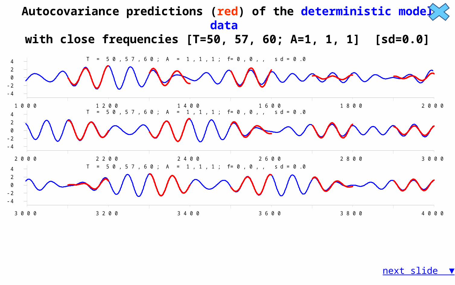
Autocovariance predictions (red) of the deterministic model data with close frequencies [T=50, 57, 60; A=1, 1, 1] [sd=0.0]

1000 1200 1400 1600 1800 2000

-4

-2

0

2

4 T = 50, 57, 60 ; A = 1, 1 , 1 ; f=0 , 0 , , sd=0.0

2000 2200 2400 2600 2800 3000

-4

-2

0

2

4 T = 50 , 57, 60 ; A = 1, 1 , 1 ; f=0 , 0 , , sd=0.0

3000 3200 3400 3600 3800 4000

-4

-2

0

2

4 T = 50 , 57, 60 ; A = 1, 1 , 1 ; f=0 , 0 , , sd=0.0

next slide ▼

Autocovariance (red) and autoregressive (green) predictions of the model data with many frequencies T=10, 15, 20, 25, 40, 60, 90, 120, 180; A=1 (all); f=0 (all) (noise sd=0,1,2)

0 100 200 300 400 500 600 700 800 900 1000 1100 1200

-4

0

4

T = 10, 15 , 20 . 25, 40 , 60, 90, 120, 180; A = 1 (a ll) f = 0 (a ll), sd=0.0

0 100 200 300 400 500 600 700 800 900 1000 1100 1200

-4

0

4

T = 10, 15, 20. 25, 40 , 60, 90, 120, 180; A = 1 (a ll) f = 0 (a ll), sd=1.0

next slide ▼

0 100 200 300 400 500 600 700 800 900 1000 1100 1200

-4

0

4

T = 10, 15, 20. 25, 40 , 60, 90, 120, 180; A = 1 (a ll) f = 0 (a ll), sd=2.0

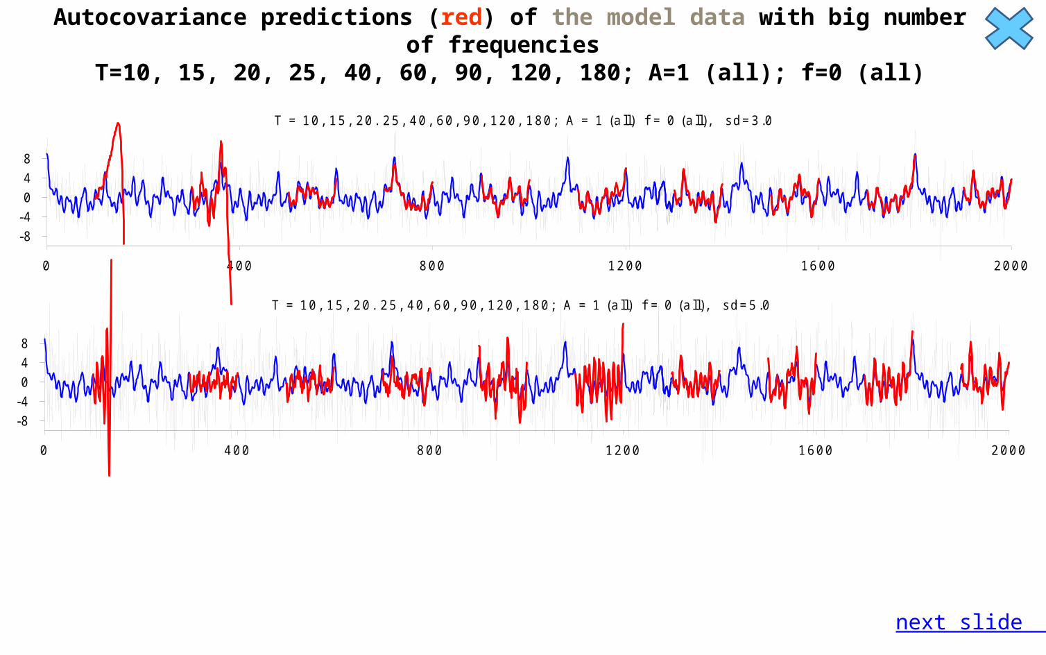
Autocovariance predictions (red) of the model data with big number of frequencies T=10, 15, 20, 25, 40, 60, 90, 120, 180; A=1 (all); f=0 (all)

0 400 800 1200 1600 2000

-8

-4

0

4

8

T = 10, 15 , 20 . 25, 40 , 60 , 90, 120, 180; A = 1 (a ll) f = 0 (a ll), sd=5.0

0 400 800 1200 1600 2000

-8

-4

0

4

8

T = 10, 15 , 20 . 25, 40 , 60 , 90, 120, 180; A = 1 (a ll) f = 0 (a ll), sd=3.0

next slide ▼

Autocovariance (red) and autoregressive (green) predictions of the seasonal model data with random walk phase: Random walk computed by integration of white noise (sd=1o, 2o , 3o)

next slide ▼

0 2000 4000 6000 8000 10000 12000

-2

-1

0

1

2 T=365.24, A =1.0 (sd=0.1), f= (random w alk, sd=1.0)

0 2000 4000 6000 8000 10000 12000

-2

-1

0

1


0 2000 4000 6000 8000 10000 12000

-2

-1

0

1


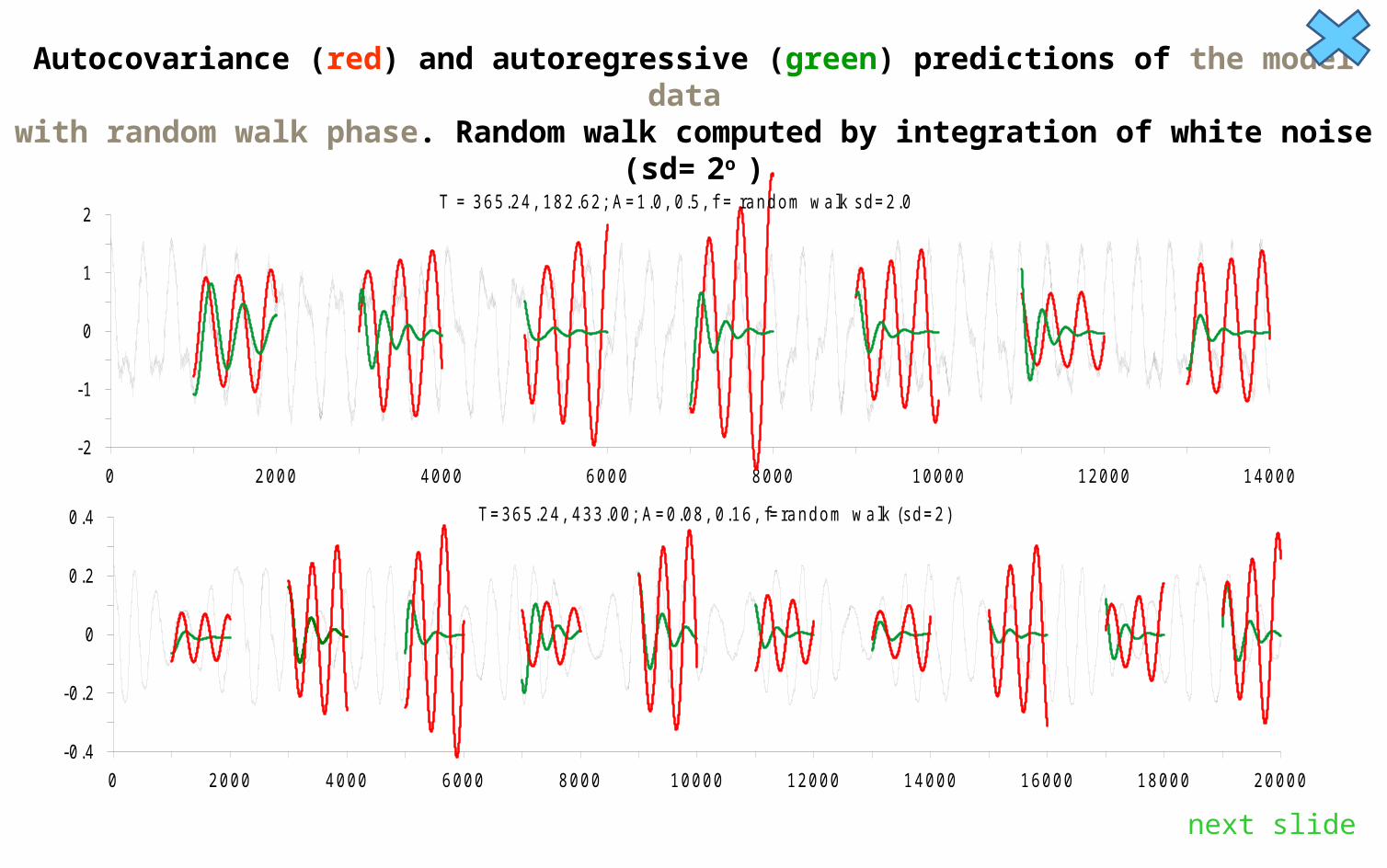
Autocovariance (red) and autoregressive (green) predictions of the model data with random walk phase. Random walk computed by integration of white noise (sd= 2o )

next slide ▼

0 2000 4000 6000 8000 10000 12000 14000

-2

-1

0

1

2T = 365.24, 182.62; A=1.0, 0.5, f = random w alk sd=2.0

0 2000 4000 6000 8000 10000 12000 14000 16000 18000 20000

-0.4

-0.2

0

0.2

0.4 T=365.24, 433.00; A =0.08, 0 .16, f= random w alk (sd=2)

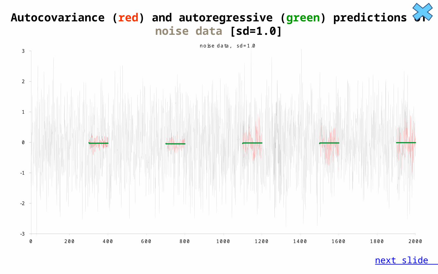
Autocovariance (red) and autoregressive (green) predictions of noise data [sd=1.0]

next slide ▼

0 200 400 600 800 1000 1200 1400 1600 1800 2000

-3

-2

-1

0

1

2

3noise data , sd=1.0

Conclusions• The input time series for computation of autocovariance and autoregressive

predictions should be stationary, because both methods need autocovarince estimates that should be functions of time lag only.

• The autocovariance prediction formulae do not able to estimate the appropriate value of prediction amplitude, so it must be rescaled using constant value of the amplitude coefficient β estimated empirically.

• The accuracy of the autocovariance predictions depend on the length of time series and noise level in data. The predictions may become unstable and when the length of time series decreases, the noise level is big or the frequencies of oscillations are too close.

• The autoregressive prediction is not recommended for noisy time series, but it can be applied when oscillation frequencies are close.

• The autocovariance prediction method can be applied to noisy time series if their length is long enough, but it is not recommended if frequencies of oscillations are close.

• The autocovariance predictions of noise data are similar to noise with smaller standard deviations and autoregressive predictions are close to zero.

next slide

References• Barrodale I. and Erickson R. E., 1980, Algorithms for least-squares linear prediction and

maximum entropy spectral analysis - Part II: Fortran program, Geophysics, 45, 433-446. • Brzeziński A., 1994, Algorithms for estimating maximum entropy coefficients of the

complex valued time series, Allgemeine Vermessungs-Nachrichten, Heft 3/1994, pp.101-112, Herbert Wichman Verlag GmbH, Heidelberg.

• Kosek W., 1993, The Autocovariance Prediction of the Earth Rotation Parameters. Proc. 7th International Symposium ”Geodesy and Physics of the Earth” IAG Symposium No. 112, Potsdam, Germany, Oct. 5-10, 1992. H. Montag and Ch. Reigber (eds.), Springer Verlag, 443-446.

• Kosek W., 1997, Autocovariance Prediction of Short Period Earth Rotation Parameters, Artificial Satellites, Journal of Planetary Geodesy, 32, 75-85

• Kosek W., 2002, Autocovariance prediction of complex-valued polar motion time series, Advances of Space Research, 30, 375-380.

next slide

Acknowledgments

Paper was supported by the Polish Ministry of Science and Education, project UMO-2012/05/B/ST10/02132 under the leadership of Prof. A. Brzeziński.