Comparison of the Aluminium Versus Steel … of the Aluminium Versus Steel Telecommunication Towers in Stochastic ... stage and composite character ... and since 3D bar and beam elements

Mechanics and Mechanical Engineering

Vol. 15, No. 2 (2011) 101–116c© Technical University of Lodz

Comparison of the Aluminium Versus SteelTelecommunication Towers in Stochastic

Finite Element Method Eigenvibrations Analysis

Marta SoleckaMarcin KaminskiJacek Szafran

Department of Structural Mechanics,Faculty of Civil Engineering,

Architecture and Environmental Engineering,Technical University of ÃLodz,

Al. Politechniki 6, 90-924 ÃLodz,Poland

Received (15 November 2010)

Revised (21 January 2011)

Accepted (29 April 2011)

The main aim of this paper is to make a comparison of the eigenfrequencies of the hightelecommunication towers alternatively manufactured using the stainless steel and thealuminium components. It is provided each time assuming that the Young modulusof the applied material is the Gaussian input random variable and using the general-ized stochastic perturbation method using the global version of the Response FunctionMethod. Up to the fourth order probabilistic moments and characteristics are computedin the three dimensional Finite Element Method model of the tower composed from thecontinuous linear elastic edge beams spanned by the large number of the linear elasticbars. A computational part of the work is made using the hybrid usage of the computeralgebra system MAPLE and the FEM engineering package ROBOT used widely in thecivil engineering practice.

Keywords: Stochastic dynamics, Stochastic Finite Element Method, response functionmethod, stochastic perturbation technique

1. Introduction

The telecommunication towers undoubtedly belong to the class of the lightweightstructures exhibited to the stochastic influence of the wind blow and since that,their reliability needs to be evaluated with respect to the strength, to maximumdeflections and rotations as well as to the eigenfrequencies. The uncertainty in thestructural response of the towers and masts in general follows the quasi–periodicand temporary ice covers increasing both mass and effective surfaces of the struc-tural elements, temperature fluctuations leading to the significant thermal stresses

102 Solecka, M., Kaminski, M. and Szafran, J.

not necessarily uniformly influencing the entire structure (concerning dominatingsouthern exposure to the sun heating). The separate role in overall uncertainty mag-nitude play the geometrical imperfections in the elements connections (especiallyin welds) and the elements themselves since material defects following productionsstage and composite character of the micro– and nanostructure. Because aluminiumhas decisively more micro–compounds in its total volume, randomization of the ba-sic material properties is even more justified than for stainless steels and, finally, arandom dispersion of those properties needs to be significantly larger.

It is known from the engineering practice that the telecommunication structures(towers, masts and antennas) designing and manufacturing is still relatively new andthe very modern area for the engineers and scientists because the development of themobile phones is still in progress and may demand the brand new extensions in thenearest future. Therefore, an optimization of the relevant supporting structures’shape and the materials’ design is still an ongoing development – an example isalternative usage of the aluminium and steel based supporting towers.

On the other hand, the engineering reliability analysis is still being developed,concerning at least the demands of the Eurocodes and, at the same time, acquisitionof various stochastic methods in engineering practice [1, 8–11]. It is widely known,that the reliability measured with some indices must be computed not only forthe load capacity and maximum deflections of some structures but also for theirvibrations and fatigue under dynamic loads, which needs further, more advancedstochastic computer methods.

These are the main reasons to investigate the matter of comparison of the alu-minium and steel manufactured telecommunication structures in the presence ofuncertainty in material properties of the structural components. We study randomfluctuations of the eigenvibrations modes for the same towers made of steel and,than of aluminium to discuss in this context their reliability issues and we assume inthis case that the Young modulus of both materials is a truncated Gaussian randomvariable with the given expected value and the coefficient of variation being an extrainput parameter to this analysis. The generalized stochastic perturbation techniqueis employed to achieve this goal since the expected time savings (with respect to theMonte–Carlo technique) and a determination of up to the fourth order probabilisticmoments and coefficients (in addition to the other stochastic methods).

Computational part is provided using the Finite Element Method engineeringsystem ROBOT, where all the eigenfrequencies are determined with respect to theinitially modified Young moduli of both towers. Further computations of the re-sponse functions, their automatic differentiation, the probabilistic moments and thecoefficients as well as their visualization are provided with the use of computer al-gebra system MAPLE. This analysis is planned to be extended towards a full ve-rification of the static and dynamic reliability, buckling fragility as well as includingof the fatigue and ageing phenomena into the overall structure mathematical andcomputational models.

Comparison of the Aluminium Versus Steel... 103

2. Variational formulation

Let us consider the following linear elasto–dynamic problem consisting of [6]

• the equations of motion

DTσ + f = ρu, x ∈ Ω , τ ∈ [t0,∞) (1)

• the constitutive equations

σ = Cε, x ∈ Ω , τ ∈ [t0,∞) (2)

• the geometric equations

ε = Du, x ∈ Ω, τ ∈ [t0,∞) (3)

• the displacement boundary conditions

u = u, x ∈ ∂Ωu, τ ∈ [t0,∞) (4)

• the stress boundary conditions

Nσ = t, x ∈ ∂Ωσ, τ ∈ [t0,∞) (5)

• the initial conditions

u = u0, u = ˆu0, τ = t0 (6)

It is assumed that all the state functions appearing in this system are sufficientlysmooth functions of the independent variables x and τ . Let us consider the variationu(x, τ) in some time moment τ = t denoted by δu(x, τ). Using the above equationsone can show that

−∫

Ω

(DTσ + f − ρu)TδudΩ +

∫

∂Ωσ

(Nσ − t)T

δud(∂Ω) = 0 (7)

Assuming further that the displacement function u(x,t) has known values at theinitial moment u (x, t1) = 0 and at the end of the process u (x, t2) = 0, so that thevariations of this function also equal 0 at those time moments

δu (x, t1) = 0, δu (x, t2) = 0 (8)

Integrating by parts with respect to the variables x and τ we can obtain that

t2∫

t1

[δT−∫

Ω

σTδεdΩ +∫

Ω

fTδudΩ +∫

∂Ω

tTδud(∂Ω)]dτ = 0 (9)

where the kinetic energy of the region Ω is defined as

T =12

∫ρuTudΩ (10)

104 Solecka, M., Kaminski, M. and Szafran, J.

We also notice that

δε = Dδu, x ∈ Ω , τ ∈ [t0,∞) (11)

Next, we introduce the assumption that the mass forces f and the surface loadingst are independent from the displacement vector u, which means that the externalloadings do not follow the changes in the domain initial configuration. Therefore,equation (9) can be modified to the following statement:

δ

t2∫

t1

(T − Jp) dτ = 0 (12)

where Jp means the potential energy stored in the entire domain Ω

Jp = U −∫

Ω

fTudΩ−∫

∂Ωσ

tTud(∂Ω) = 0 (13)

whereas the variation is determined with respect to the displacement function andU is the elastic strain energy given by the formula

U = 12

∫Ω

εTCεdΩ (14)

It is well known that the equation (12) represents the Hamilton principle widelyused in structural dynamics in conjunction with the Finite Element Method ap-proach.

3. Computational implementation

Let us consider a discretization of the displacement field u(x, τ)using the followingforms:

uα3x1(x,τ) ∼= ϕ3xN(e)(x)qα

N(e)x1(τ), uα3x1(x,τ) ∼= Φ3xN (x)rα

Nx1(τ) (15)

where q is a vector of the generalized coordinates for the considered finite element,r is a vector for the generalized coordinates of the entire discretized system, N(e) isthe total number of the eth finite element degrees of freedom; N is the total numberof degrees of freedom in the structure model. The generalized coordinates vector forthe entire structure model is composed from the finite element degrees of freedomand the transformation matrix as

rαNx1 = aNxN(e)q

αN(e)x1 (16)

ϕ and Φ are the corresponding shape function matrices (local and global). Contraryto the classical formulations of both FEM and the perturbation-based StochasticFinite Element Method [2,3,6], we introduce here the additional index α=1,. . . ,Mto distinguish between various solutions of the elastodynamic problem necessaryto build up the response function (around the mean value of the input randomparameter).

Comparison of the Aluminium Versus Steel... 105

The strain tensor can be expressed as

εα6x1(x,τ) = B6xN(e)(x)qα

N(e)x1(τ) = B6xN (x)rαNx1(τ) (17)

The discretized version of the Hamilton’s principle is obtained as

δ

t2∫

t1

(12

E∑e=1

qαT mαN(e)xN(e)

qα − 12

E∑e=1

qαT kαN(e)xN(e)

qα +E∑

e=1QαT

N(e)qα

)dτ = 0

(18)and hence

δ

t2∫

t1

(12 r

αT Mαrα − 12r

αT Kαrα + RαT rα)dτ = 0 (19)

The global mass matrix is defined as

MαNxN =

∫

Ω

ρα(x)BTNx6(x)B6xN (x)dΩ (20)

so that all partial derivatives of it with respect to random Young modulus equal to0; the global stiffness matrix equals to

KαNxN =

∫

Ω(e)

BTNx6C

α6x6B6xNdΩ (21)

and since 3D bar and beam elements are used in further computations (as thelinearly dependent on Young modulus), only the first partial derivatives differ from0. Henceforth, equation (19) can be rewritten with those substitutions as

rαTMαδr−∫ t2

t1

(rαTMα + rαTKα −RαT)δr dτ = 0 (22)

Considering the assumptions that

δr(t1) = 0, δr(t2) = 0 (23)

we finally obtain the dynamic equilibrium system

Mαrα + Kαrα = Rα (24)

which represents the equations of motion of the discretized system. When we com-plete this equation with the component Cα

NxNrαNx1 getting

Mαrα + Cεrα + Kαrα = Rα (25)

then we decompose the damping matrix as

Cα = α0Mα + α1Kα (26)

where the coefficients α0 and α1 are determined using the specific eigenfunctionsfor this problem, so that

106 Solecka, M., Kaminski, M. and Szafran, J.

Mαrα + α0Mαrα + α1Kαrα + Kαrα = Rα (27)

where no summation over the doubled indices α is applied here. As it is known [2],the case of the undamped free vibrations leads to the following algebraic system:

Mαrα + Kαrα = 0 (28)

and the solution rα = Aα sin ωαt leads to the relation

−MαAαω2α sin ωαt + KαAα sinωαt = 0 (29)

so that for sin ωαt 6= 0 and Aα 6= 0 there holds

−Mαω2α + Kα = 0 (30)

4. The stochastic perturbation–based approach in the eigenproblems

4.1. The stochastic Taylor expansion with random coefficients

Let us introduce the random variable b ≡ b (ω) and its probability density functionas p(b). Then, the expected values and the mth central probabilistic moment aredefined as

E [b] ≡ b0 =

+∞∫

−∞bp (b) db, µm (b) =

+∞∫

−∞(b− E[b])m

p (b) db (31)

The basic idea of the stochastic perturbation approach is to expand all the inputvariables and the state functions via Taylor series about their spatial expectationsusing some small parameter ε > 0. In case of random quantity e = e(b), thefollowing expression is employed [4,7]:

e = e0 +∞∑

n=1

1n!ε

n ∂ne∂bn (∆b)n (32)

where

ε∆b = ε(b− b0

)(33)

is the first variation of b about b0. Symbol (.)0 represents the function value (.)taken at the expectation b0, while (.),b,(.),bb denote the first and the second partialderivatives with respect to b evaluated at b0, respectively. Let us analyze furtherthe expected values of any state function f(b) defined analogously to the formula(3) by its expansion via Taylor series with a given small parameter ε as follows:

E [f (b) ; b] =

+∞∫

−∞f(b)p (b) db =

+∞∫

−∞

(f0 +

∞∑n=1

1n!ε

nf (n)∆bn

)p (b) db (34)

Comparison of the Aluminium Versus Steel... 107

Let us remind that this power expansion is valid only if the state function is an-alytic in ε and the series converge and, therefore, any criteria of convergence shouldinclude the magnitude of the perturbation parameter; perturbation parameter istaken as equal to 1 in numerous practical computations. From the numerical pointof view, the expansion provided by the formula (32) is carried out for the summationover the finite number of components. Now, let us focus on an analytical derivationof the probabilistic moments for the structural response function. It is easy to provethat the general 6th order expansion results in the formula

E [f (b)] = f0(b) + ε∆b∂f

∂b+ 1

2ε2µ2 (b) ∂2f∂b2 + 1

3!ε3µ3(b)∂3f

∂b3

(35)

+ 14!ε

4µ4(b)∂4f∂b4 + 1

5!ε5µ5(b)∂5f

∂b5 + 16!ε

6µ6(b)∂6f∂b6

where for Gaussian variables the even components need to be dropped off. Thanksto such an extension of the random output, any desired efficiency of the expectedvalues as well as higher probabilistic moments can be achieved by an appropriatechoice of the distribution parameters. Similar considerations lead to the 4th orderexpressions for a variance; there holds

V ar (f(b)) = ε2µ2 (b)∂f

∂b

∂f

∂b+ ε4µ4 (b)

(14

∂2f∂b2

∂2f∂b2 + 2

3!∂f∂b

∂3f∂b3

)

(36)

+ε6µ6(b)((

13!

)2 ∂3f

∂b3

∂3f

∂b3+ 1

4!∂4f∂b4

∂2f∂b2 + 2

5!∂5f∂b5

∂f∂b

)

The third order probabilistic moments are derived including the lowest orders onlyas

µ3 (f (b)) =

+∞∫

−∞(f (b)− E[f(b)])3 p (b) db

=

+∞∫

−∞

(f0 + ε

∂f

∂b∆b + ...− E[f(b)]

)3

p (b) db (37)

=

+∞∫

−∞

(ε∂f

∂b∆b + 1

2ε2 ∂2f∂b2 ∆b∆b + ...

)3

p (b) db

∼= 32ε4µ4(b)

(∂f∂b

)2∂2f∂b2 + 1

8ε6µ6(b)(

∂2f∂b2

)3

108 Solecka, M., Kaminski, M. and Szafran, J.

Finally, the fourth probabilistic moment is approximated with the first few per-turbation terms as

µ4 (f (b)) =

+∞∫

−∞(f (b)− E[f(b)])4 p (b) db

=

+∞∫

−∞

(f0 + ε

∂f

∂b∆b + ...− E[f(b)]

)4

p (b) db (38)

= ε4µ4(b)(

∂f

∂b

)4

+ 32ε6µ6(b)

(∂f∂b

∂2f∂b2

)2

+ 116ε8µ8(b)

(∂2f∂b2

)4

Let us mention that it is necessary to multiply in each of these equations bythe relevant order probabilistic moments of the input random variables to get thealgebraic form convenient for any symbolic computations. Therefore, this methodin its generalized form is convenient for all the random distributions, where theabove mentioned moments may be analytically derived (or at least computed for aspecific combination of those distributions parameters). Finally, one may recoverthe kurtosis and the skewness after their well–known definitions as

κ (f (b)) =µ4 (f (b))σ4 (f (b))

− 3, β (f (b)) =µ3 (f (b))σ3 (f (b))

(39)

and, independently, the reliability index for the particular eigenfrequencies as

R (f (b)) =E

(f − fα

)

σ(f − fα

) (40)

where the pair(f ; fα

)denotes the induced frequency of the vibrations and the addi-

tional eigenfrequency. The relevant civil engineering codes state that this differencecannot be smaller than 25% of the eigenfrequency, so that Eqn. (40) may serve forthe straightforward estimation of the reliability for the structures subjected to thedynamic excitations.

4.2. Eigenfrequencies determination via the response function method

As shown during derivation of equations for the generalized perturbation basedapproach, one of the most complicated issues is a reliable numerical determination ofup to nth order partial derivatives of the structural response function with respect tothe randomized parameter. It is possible to determine this function first by multiplesolutions of the boundary value problem around the expectation of the randomparameter to complete this task. The response function for each eigenvalue is builtup from uniform symmetric discretization in the neighborhood of this expectation,with equidistant intervals. A set of classical deterministic re–computations of theall the components of the eigenvalues vector leads to the final formation of theresponses function for all ωα. That is why we consider further a problem of the

Comparison of the Aluminium Versus Steel... 109

unknown response function approximation by the following polynomial of n-1 order[5]:

ωα = A(α)1 bn−1 + A

(α)2 bn−2 + ... + A(α)

n b0 (41)

having the values of this function determined computationally for n different argu-ments. With this representation, the algebraic system of equations is formed

A(α)1 bn−1

1 + A(α)2 bn−2

1 + ... + A(α)n b0

1 = ωα(1)

A(α)1 bn−1

2 + A(α)2 bn−2

2 + ... + A(α)n b0

2 = ωα(2)

...

A(α)1 bn−1

n + A(α)2 bn−2

n + ... + A(α)n b0

n = ωα(n)

(42)

where the coefficients ωα(i) for i=1,. . . ,n denote the approximated function valuesin ascending order of the arguments bi. Therefore, the following algebraic systemof equations is formed to determine the polynomial coefficients A

(α)i :

bn−11 bn−2

1 ... b01

bn−12 bn−2

2 b02

... ... ...bn−1n bn−2

n ... b0n

A(α)1

A(α)2

...

A(α)n

=

ωα(1)

ωα(2)

...ωα(n)

(43)

The crucial point in this method is a proper determination of the set of inputparameters

b01, ..., b

0n

inserted into this equation. This determination is started

with a choice of the computational domain [b−∆b, b + ∆b], where 2∆b = 0.05b.Then, this domain is subdivided into the set of equidistant n–1 intervals with thelength ∆b(m,m+1) = 2∆b

n−1 for any m=1,..,n-1. So that assuming that b0 = b−∆b itis obtained that bm = b−∆b + m 2∆b

n−1 . Let us note that since this linear system ofequations is non–symmetric, its solution cannot be done by the integration with theFEM solver, and some separate numerical procedure based on the Gauss–Jordanelimination scheme must be employed. The unique solution for this system makesit possible to calculate up to the nth order ordinary derivatives of the homoge-nized elasticity tensor with respect to the parameter b at the given b0 as 1st orderderivative

∂ωα

∂b= (n− 1)A

(α)1 bn−2 + (n− 2) A

(α)2 bn−3 + ... + A

(α)n−1 (44)

2nd order derivative

∂2ωα

∂b2= (n− 1) (n− 2)A

(α)1 bn−3 + (n− 2) (n− 3) A

(α)2 bn−4 + ... + A

(α)n−2 (45)

kth order derivative

∂kωα

∂bk=

k∏

i=1

(n− i) A(α)1 bn−k +

k∏

i=2

(n− i) A(α)2 bn−(k+1) + ... + A

(α)n−k (46)

110 Solecka, M., Kaminski, M. and Szafran, J.

Providing that the response function of the structural eigenvalue has a singleindependent argument, that is, the input random variable of the problem, it ispossible to employ the stochastic perturbation technique based on the Taylor rep-resentation to compute up to the mth order probabilistic moments µm(ωα). It isclear from the derivation above that to complete the mth order approximation weneed to solve the initial deterministic problem m times, with its number of degreesof freedom and a single system of algebraic equations mxm, to find a single responsefunction. Including the formulas above for the derivatives of the response functionin a definition of the probabilistic moments, one can determine the expectations,variances as well as any order random characteristics of the structural response.

5. Numerical illustrations

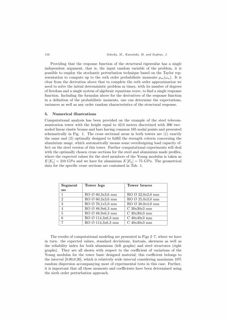
Computational analysis has been provided on the example of the steel telecom-munication tower with the height equal to 42.0 meters discretized with 396 two–noded linear elastic beams and bars having common 165 nodal points and presentedschematically in Fig. 1. The cross–sectional areas in both towers are (1) exactlythe same and (2) optimally designed to fulfill the strength criteria concerning thealuminium usage, which automatically means some overdesigning load capacity ef-fect on the steel version of this tower. Further computational experiments will dealwith the optimally chosen cross–sections for the steel and aluminium made profiles,where the expected values for the steel members of the Young modulus is taken asE [Es] = 210 GPa and we have for aluminium E [Ea] = 75 GPa. The geometricaldata for the specific cross–sections are contained in Tab. 1.

Segmentno

Tower legs Tower braces

1 RO Ø 60,3x3,6 mm RO Ø 22,0x2,0 mm2 RO Ø 60,3x3,6 mm RO Ø 25,0x3,0 mm3 RO Ø 76,1x5,0 mm RO Ø 38,0x4,0 mm4 RO Ø 88,9x6,3 mm C 30x30x3 mm5 RO Ø 88,9x6,3 mm C 30x30x3 mm6 RO Ø 114,3x6,3 mm C 40x40x3 mm7 RO Ø 114,3x6,3 mm C 40x40x3 mm

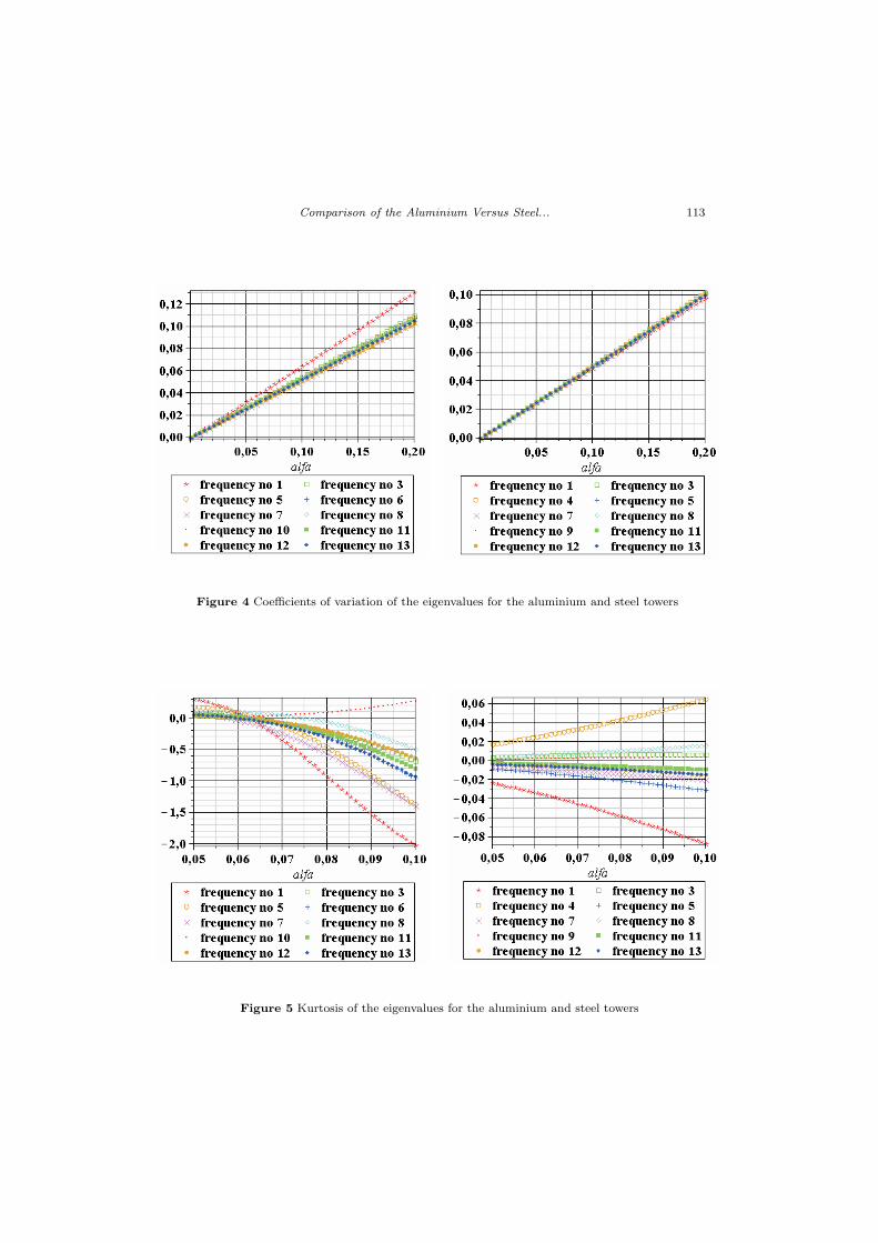
The results of computational modeling are presented in Figs 2–7, where we havein turn: the expected values, standard deviations, kurtosis, skewness as well asthe reliability index for both aluminium (left graphs) and steel structures (rightgraphs). They are all shown with respect to the coefficient of variations of theYoung modulus for the tower basic designed material; this coefficient belongs tothe interval [0.00,0.20], which is relatively wide interval considering maximum 10%random dispersion accompanying most of experimental tests in this case. Further,it is important that all those moments and coefficients have been determined usingthe sixth order perturbation approach.

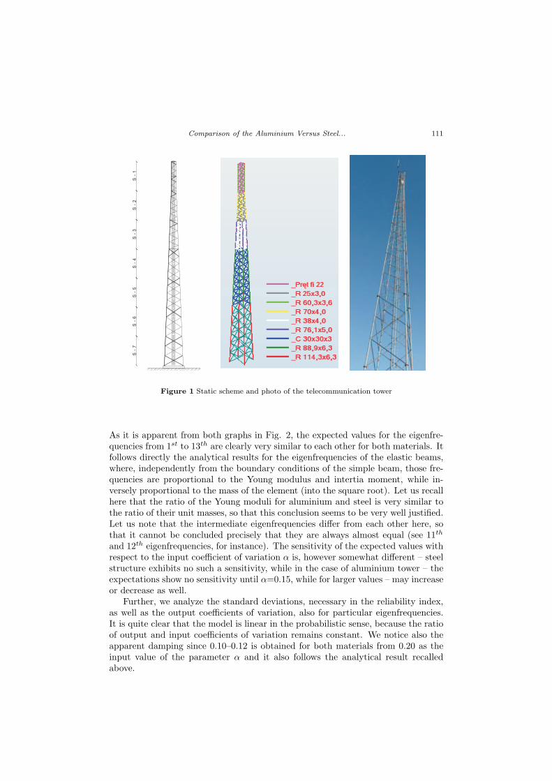
Comparison of the Aluminium Versus Steel... 111S

-1

S-

2S

-3

S-

4S

-5

S-

6S

-7

Figure 1 Static scheme and photo of the telecommunication tower

As it is apparent from both graphs in Fig. 2, the expected values for the eigenfre-quencies from 1st to 13th are clearly very similar to each other for both materials. Itfollows directly the analytical results for the eigenfrequencies of the elastic beams,where, independently from the boundary conditions of the simple beam, those fre-quencies are proportional to the Young modulus and intertia moment, while in-versely proportional to the mass of the element (into the square root). Let us recallhere that the ratio of the Young moduli for aluminium and steel is very similar tothe ratio of their unit masses, so that this conclusion seems to be very well justified.Let us note that the intermediate eigenfrequencies differ from each other here, sothat it cannot be concluded precisely that they are always almost equal (see 11th

and 12th eigenfrequencies, for instance). The sensitivity of the expected values withrespect to the input coefficient of variation α is, however somewhat different – steelstructure exhibits no such a sensitivity, while in the case of aluminium tower – theexpectations show no sensitivity until α=0.15, while for larger values – may increaseor decrease as well.

Further, we analyze the standard deviations, necessary in the reliability index,as well as the output coefficients of variation, also for particular eigenfrequencies.It is quite clear that the model is linear in the probabilistic sense, because the ratioof output and input coefficients of variation remains constant. We notice also theapparent damping since 0.10–0.12 is obtained for both materials from 0.20 as theinput value of the parameter α and it also follows the analytical result recalledabove.

112 Solecka, M., Kaminski, M. and Szafran, J.

Figure 2 Expected values of the eigenvalues for the aluminium and steel towers

Figure 3 Standard deviations of the eigenvalues for the aluminium and steel towers

Comparison of the Aluminium Versus Steel... 113

Figure 4 Coefficients of variation of the eigenvalues for the aluminium and steel towers

Figure 5 Kurtosis of the eigenvalues for the aluminium and steel towers

114 Solecka, M., Kaminski, M. and Szafran, J.

Figure 6 Skewness of the eigenvalues for the aluminium and steel towers

Figure 7 Reliability index in eigenvibrations analysis of the aluminium and steel towers

Comparison of the Aluminium Versus Steel... 115

Higher damping is noticed for the steel tower, where additionally the results forparticular eigenfrequencies are less dispersed than for the aluminium structures.

Kurtosis given in Fig. 5, however, is apparently different for both materials –they both start from 0 for the input coefficient of variation close to 0 to some mostlynegative values for the aluminium and relatively small positive as well as negativevalues in the case of steel (closer to 0). Contrary to the previous moments andcoefficients, the fourth order quantities are computed with lower accuracy lost withlarger values of α, so that the results are restricted to the 10% input random disper-sion; this is also the case of skewness as the result of the third order approximations(see Fig. 6). These skewnesses exhibit similar properties as the kurtosis – in thesense that they have smaller absolute values for steel tower than for the aluminiumone. Steel structure shows a linear interrelation between output skewness and in-put coefficient of variation of the Young modulus. This is absolutely not the caseof aluminium tower eigenfrequencies, where this interrelation does not seem to belinear, while the minimum values apparently differ from 0. Trying to generalizethose results one may notice that Gaussian Young modulus of the tower resultin the eigenfrequencies being almost Gaussian, when the tower is made of steel,whereas the final distributions of aluminium eigenfrequencies are more distant fromthe Gaussian one (due to negative skewness and kurtosis).

Finally, we study the variations of the reliability index as the function of theinput uncertainty for α belonging to the interval [0.0, 0.10]. The results obtainedfor both materials are quite similar – the larger input coefficient of variation, thesmaller final reliability index value. It is known from the Eurocode 0 regulations,that the unconditional structural safety is preserved in the case of reliability indexlarger than about 4.5. Fig. 7 shows clearly that the safety margin for both struc-tures is rather small, because this limit value is reached for the eigenfrequencieslower or equal to 10th at the input coefficient α = 0.07 (for aluminium) and forα = 0.07 (in the case of steel). This structure is, however, never safe in the viewof higher eigenfrequencies, because for the entire variability of input coefficient ofvariation the final reliability index is equal or smaller than 4. It is seen that thestructure safely designed according to the strength and deflections condition notnecessarily exhibit full safety in the view of eigenvibrations analysis. One needs toremember also that usually input coefficient of variation increases together with theexploitation time, so that the graphs, provided may be directly interpreted duringfull stochastic reliability analysis, after a sensible calibration of time versus inputrandom dispersion level.

6. Concluding remarks

The main result of the analyses presented in this paper is that the eigenfrequenciesexpectations computed for aluminium and steel towers are very close to each other,which follows almost identical interrelations of the Young moduli and densities ofboth materials. Both materials exhibit probabilistic damping in free vibrationsanalysis decreasing almost twice the input uncertainty level. The probabilistic dis-tributions for all eigenfrequencies in the steel tower are essentially closer to theGaussian origin than for the aluminium tower, where both skewness and kurtosisshow clearly negative values. The reliability analysis is also straightforward pro-

116 Solecka, M., Kaminski, M. and Szafran, J.

cedure with the Stochastic Finite Element Method perturbation–based techniqueimplemented provided that the direct difference in–between induced frequency ofvibrations and the eigenfrequency is declared in percents with respect to this lastquantity. Otherwise, of course, full stochastic forced vibrations analysis is neces-sary, which needs further extensive developments of the SFEM procedures. Thereis no doubt that the computer algebra system plays the crucial role in the com-putational strategy – one may try to use this hybrid strategy with the responsefunction method in addition to the other probability density functions, especiallyfor the lognormal variables, where all central moments of any order have additionalanalytical forms. Otherwise, some further numerical techniques must be employedto recover those moments for the needs of specific input random variables confi-guration. The structural open research problems may be for instance the SFEManalysis of stochastic earthquake vibrations applied at the foundations of such to-wers, significantly influencing stochastic reliability of those structures.

AcknowledgmentThe second author would like to acknowledge the Research Grant NN 519 386 636

from the Polish Ministry of Science and Higher Education.

References

[1] Benaroya, H.: Random eigenvalues, algebraic methods and structural dynamic mod-els, Applied Mathematics and Computation, 52(1), 37–66, 1992.

[2] Clough, R. and Penzien, J.: Dynamics of Structures, McGraw–Hill, 1975.

[3] Hughes, T.J.R.: The Finite Element Method – Linear Static and Dynamic FiniteElement Analysis, Dover Publications, Inc., New York, 2000.

[4] Kaminski, M.: Generalized perturbation–based stochastic finite element method inelastostatics, Computers & Structures, 85(10), 586-594, 2007.

[5] Kaminski, M. and Szafran, J.: Random eigenvibrations of elastic structures bythe response function method and the generalized stochastic perturbation technique,Archives of Civil & Mechanical Engineering, 10(1), 33-48, 2010.

[6] Kleiber, M.: Introduction to the Finite Element Method (in Polish), Polish ScientificPublishers, Warszawa–Poznan, 1986.

[7] Kleiber, M. and Hien, T.D.: The Stochastic Finite Element Method, Wiley, Chich-ester, 1992.

[8] Mehlhose, S., vom Scheidt, J. and Wunderlich, R.: Random eigenvalue prob-lems for bending vibrations of beams, Zeitschrift fur Angewandte Mathematik undMechanik, 79(10), 693–702, 1999.

[9] Nair, P.B. and Keane, A.J.: An approximate solution scheme for the algebraicrandom eigenvalue problem, Journal of Sound & Vibrations, 260(1), 45–65, 2003.

[10] Pradlwater, H.J., Schueller, G.I. and Szekely, G.S.: Random eigenvalue prob-lems for large systems. Computers & Structures, 80(27), 2415–2424, 2002.

[11] Soize, C.: Random matrix theory and non-parametric model of random uncertaintiesin vibration analysis, Journal of Sound & Vibrations, 263(4), 893–916, 2003.