WSRC-RP-93-269 July 1993 / COMPARISON OF SAVANNAH RIVER SITE'S METEOROLOGICAL DATABASES(U) A. H. Weber Approved by A.L. Dbnl Research Manager Environmental Technology Section ..,_: S SAVANNAH RIVER SITE iii i i 'Westinghouse Savannah River Company Savannah River Technology Center Aikenr SC 29808 :,, 93zo$?oJIwo DtSTRIBU]'ION OF THIS DOC:LJMEN[ IS UI"4LIMIT'C'_ .j

Welcome message from author
This document is posted to help you gain knowledge. Please leave a comment to let me know what you think about it! Share it to your friends and learn new things together.
Transcript
WSRC-RP-93-269July 1993
/
COMPARISON OF SAVANNAH RIVER SITE'SMETEOROLOGICAL DATABASES(U)
A. H. Weber
Approved by
A.L. DbnlResearch ManagerEnvironmental Technology Section
. .,_:
SSAVANNAH RIVER SITE
iii i i
'Westinghouse Savannah River CompanySavannah River Technology CenterAikenr SC 29808
:,, 93zo$?oJIwo
DtSTRIBU]'ION OF THIS DOC:LJMEN[ IS UI"4LIMIT'C'_ .j
ill
Thisreportwaspreparedby theWestinghouseSavannahRiverCompany(WSRC)for theUnitedStatesDeparunentof EnergyunderConnct No. DE-AC09-89SR18035and is an accountof workperformedunder thatCOltIII_L Neither the United States Deparunent of Energy, norWSRC, nor any Of theiremployeesmakeany warranty,expressedorimplied,norassumeanylegal liabilityorresponsibilityfortheaccuracy,completeness,orusefulness,of anyinformation,apparatus,orproductorprocessdisclosedhereinor representsthatitsusewill not_ge privatelyownedrighL_,Referencehereintoanyspecificcommercial product,prtx:ess,or service by trademark,name, manufacturer,or otherwise does notnecessarilyconstituteor implyendorsement,recommendation,orfavoringof thesame by WSRCor bythe UnitedStatesGovernmentor anyagency thereof.The views andopinions of the authorsexpressedherein do notnecessarily stateor reflect thoseof the U.S. Governmentor any agency thereof.
Comparison of Savannah River Site's Five.Year Meteorological Databases
Executive Summary.
A five-year meteorological database from the 61-meter, H-Area tower for theperiod 1987-91 was compared to an earlier database for the period 1982-86. Theamount of invalid data for the newer 87-91 database was one third that for theearlier database. The data recovery percentage for the last four years of the 87-91database was well above 90%. As described in the background sections,considerable effort was necessary to fiU in for missing data periods for the newerdatabase for the H-Area tower. Therefore, additional databases that have beenprepared for the remaining SRS meteorological towers have had missing anderroneous data flagged, but not replaced. The F-Area tower's database was usedfor cross-comparison purposes because of its proximity to H Area.
Statistical tests were used to compare the frequency of occurrence and the meanwind speeds for the 82-86 and 87-91 databases. These tests are extremelysensitive because of the large number (-35,000-45,000) of hourly observationsin the data sets. The tests show statistically significant differences in thefrequency of occurrence of winds for the H-Area tower for all seven Pasquillstability classes, two of sixteen wind directions sectors (IVand S), and four of sixwind speed categories. The mean wind speeds between the two time periodscompared more favorably, with only G stability category showing a statisticallysignificant difference.
The differences in frequency of occurrence for stability classes may be caused byclimatic changes, such as a 0.6°C temperature increase between 1982 and 1991,the period during which data was collected. The differences in the north windsector were probably due to a coding fault and the instrument maker's design forthe wind direction instruments. The differences found for the south wind sector
Comparison of Savannah River Site's Five-Year Meteorological Databases
and all wind speed classes are probably either due to natural climatic variation,statistical variability, or differences in the data screening methods used for thetwo time.periods. The fact that the mean wind speeds are significantly differentfor the G stah;lity class may be due to the use of different data screening methodsfor the two timeperiods.
A baa's was provided for future comparisons by examining wind speed powerspectra and by stratifying the data by season and time of day. The wind speedpower spectra showed expected yearly, 3-5 day, 24 and 12 hour peaks. Peaksoccurring at periods of 8 hours and 32-26 days have not as yet been explained.The stratification by season showed a trimodal spring pattern with dominantwinds from the S and SSE. During summer, winds from the N become veryinfrequent and the S to W wind sectors are dominant. A dramatic shift occurs inthe autumn to winds from the NE and ENE. In the winter there is a very narrowpeak of windsfrom the NE and a broad quadrant of windsfrom the S-WNW witha local maxima of winds from the W. Winds from the N and NNW are aboutequallyfrequent for all seasons except summer.
The evening and midnight patterns during the spring and summer are verysimilar, all showing minima out of the N quadrant and maxima out of the Squadrant. Spring and summer mornings and middays resemble one another withmaxima out of the WSW and NE or ENE. Pre-dawn and morning periods in theautumn are similar with local maxima from the NE. Spring and summerafternoon patterns are similar with maxima in the S to W quadrant. Duringspring and summer the pre-dawn periods have winds which are fairly uniformlydistributed with minimafrom the WNW toN sectors.
The primary purpose of this report is to compare the H-Tower databases for 82-86 and 87-91. Statistical methods enable the use of probability statements to bemade concerning the hypothesis of no chfferences between the distributions of thetwo time periods, assuming each database is a random samplefrom its respectivedistribution. This assumption is required for the statistical tests to be valid. Anumber of statistical comparisons can be made between the two data sets, eventhough the 82-86 database exists only as distributions of frequency and meanspeed.
2 93XOJTO.MWO
Comparison of Savannah River Site'sFive.YearMeteorologicalDatabases
Background
In early 1992 the Environmental Technology filled fromnearbytowers, backupdatacollectedSection of the Savannah River Technology at the site (called SUM-X data), Plant Vogtle'sCenter (SRTC) completeda quality-assuredfive- mek:orological tower, or fromNational Weatheryearmeteorologicaldatabasefor the 61-meter,H- Service observations. The result of these effortsArea towerfor the period 1987-91 (Parker,et al., was a high quality database with no missing1992). The database was created for the New observations. A total of only 8.3% of the dataProduction Reactor's (NPR) safety and had to be substituted in these ways for the H-environmentalstudies. Several onsite and offsite Area tower 87-91 database. The amount ofgroups have requestedsimilar data sets since the invalid data was one third that foran earlierfiveNPR database was created. The Parker, et al. yeardatabase (L,aurinat,1987).(1992) report, provides descriptions of the datacollection, processing, and validation used in Laurinat(1987) produceda quality assuredfive-producing the database. The Savannah River year database covering the period 1982-86 forSite's (SRS) 87-91 H-Area database is unique each of the SRS Area towers. The 82-86since there are no missing data in the five year databases differfromthe 87-91 H-Towerdatabaseperiod. The data set includes a total of 43,824 in that the quality assurance tests were appliedhours of data for the five-year time period only duringcomputerprocessing usingstatistical(including one leap year). Each data entry screening algorithms. Visual data inspectioncontains wind speed, wind direction, and lateral techniques were not used. Time periods withturbulence intensity. The data entries for the missing data were not filled, consequently, theyears 1989-91 contain temperatures and dew 1982-86 data records contain missing periodspoints as well. ' whenever the data failed the computer screening
algorithms or the tower was out of service forOne.procedureused to qualityassure the 87-91 H- maintenance,damagedby lightning, etc.Towerdatabase involved plottinga time seriesoffifteen-minute records by tower for one-week The 82-86 computer screening algorithmsperiods. These one-week plots, showing all eight rejected data for failure to pass a statistical testof SRS's meteorological towers simultaneously, knownas the Dixon ratio test (Dixon, 1957), andallowed comparativechecks to be madeof the H- for large differences between lateral andArea tower both spatially and temporally, longitudina! turbulence intensities. The DixonMalfunctioning sensors and missing data could ratio test is used to detect outliers based onbe readilydistinguishedfrom validdataand time statistical similarities of the towers' distributionperiodsnoted.Invaliddam were also identifiedby (orspatial "agreement")of windspeed, direction,inspection of log books and records which or turbulence intensity during a given hour'sidentified calibration periods, maintenance time). Data was rejectedfromboth 82-86 and87-activities, and other downtimes. In addition, 91 data sets whenever voltages exceededduringthe initial, real-time computeracquisition acceptablerangesor when more than 90% of theof the data,software algorithmsare used to check possible data within a ffl'teen-minuteperiod wasdata ranges and to test the consistency of data missing. The amount of data rejected due toentries. Additional data consistency checks were application of these tests in the 82-86 databasealso used in the software which preparedthe 87- amounted to about 21% for each of the Area91 database, towers. Missing or unreadable tape archive files
accounted for an additional 2% of data beingTime periods were flaggedwhen the H-Area data incomplete. The quality assurance proceduresdid not pass the visual or computer quality used to producethe dataset resultedin about23%assurancetests, or had missing data blocks. If the missing data for each tower. However, at thelength of the flagged time interval was 1-4 hours lime this database was generated, there was no(1.1% of the total), the data was filled by linear requirementforpercentageof data recoverability.interpolation. If the time period was from 5-13 The 87-91 database, by contrast,was required tohours (0.4% of the total), data was either filled meet the DOE'scurrentguidance of 90% annualfroma nearbytower'srecords,or by interpolating data recovery for meteorological data. Newand accounting for the diurnalcycle. If the length proceduresand meteorological instrumentswereof the flagged time intervalwas from 13 hours to installed in 1987 to improve the quality and toseveral days (6.8% of the total), the data was capturea largerpercentageof meteorologicaldata.
9Jxo57oJ_4rwo 3
Comparison of Savannah River Site'sFive.YearMeteorologicalDatabases
The new proceduresand instrumentsresultedin a from later years in the table below (extractedsignificant gain in the percentage of valid data from Parker, et al., 1992). The large increasecaptured in annual data sets. This can be between 1987 and succeeding years in Table 1substantiatedby comparingthe datarecoveryrate shows the successful nature of the qualitypercentages for the 1987 wind data with those improvementprograms.
Table 1. Data recovery percentages for each year of the period 1987-91 for the H-Area meteorologicaltower.
WindData 1987 1988 1989 1990 1991 5-Yr. Ave.(Yr.)
H-Area (%) ;'/8.15 96.21 92.84 96.58 94.55 91.71
The 82-86 databaseswere convertedto frequency Additionaldatabaseswere createdlaterin 1992 fordistributionsshortly after theircreation for use in the remainingArea towers A, C, D, F, K, L, anddosimetry models. The frequency distributions P for the 87-91 time period except that missingconsist of frequenciesof occurrenceswithin each data was not filled. The applications of theseof six speed ranges (0-2, 2-4, 4-6, 6-8, 8-12, and databases did not require that the missing time12-50 m/dec), seven Pasquill-Gifford stability periods be filled, and in some instances this iscategories (A-G), and sixteen wind direction not desired. In addition, considerable effort issectors (I-N -- 16-NNW). The ,data sets also needed to provideoata for a tower when the datacontain mean wind _7_eeds(andmean wind speeds records are incomplete. The 87-91 data sets forby inverse averaging) for the same speed ranges, the remaining towers contain hourly-averagedPasquill.Gfffordcategories, and direction sectors. . data and frequency distributions. These databases(Pasquill-Gifford stability categories were exist primarily for special studies or researchdetermined from the measured latend turbulence where having a completely Idled database for theintensity according to the U. S. Nuclear entire five years is unimportant. One of these 87-Regulatory Commission Guide 1.23.) The 87-91 91 data sets for the F-Area tower was usedH-Tower database exists both as a frequency extensively in this report for cross comparisondistribution (as for the 82-86 database) and as a purposes in some of the statistical studiespermanent on-line data set, containing the described later. The earlier 82-86 database for theoriginal hourly observations. F-Area tower by Laurinat was also used for cross
comparison purposes.
Statistical Comparisons Between the 82-86 and 87-91Databases
The statistical comparisons are described in this A test was applied to the differences between thesection but more mathematical details are observed andexpected numberof observations forincludedin AppendixA. The (null) hypothesis thesixteensectors,sevenstabilitycategories,andbeing tested is: There is no difference six windspeedcategories.The squareddifferencebetween the distributions for the two between the number observed and the number
//mLJ/g£_p.dE In order to test this hypothesis, expected for both data sets can be used tothe frequencyof occurrenceandmean windspeed determine if the differences are statisticallydistributionsby sector, wind speed category, and significant.If this squareddifference is divided bystability for both periods were compared. A the expectednumberof observations,the result isprimary question to be answered -- are the the adjusted residual squared, or the cellproportional differences that exist between the contributionto the chi square. The sum of thesenumberof observations in each data set within contributions is assumed to form a chi-squarethe range of expected random statistical distributionwith degreesof freedom equal to onevariations?And similarly -- are the mean wind less thanthenumberof classes being compared.speed differences within the range of expectedrandomstatisticalvariations? The probabilityof gettinga largerchi square than
the one observed (assumingthere is no difference
4 93XOJ70.MWO
Comparison of Savannah River Site's Five.Year Meteorolol_ical Databases
between the two time periods) and the value of of getting a largerchi square is less than 0.001the chi squarestatistic are shown in Table 2 for forstability, sector,andwind speed. If one took aF-Area tower (used for comparison)and H-Area large numberof samplesfroma distributionwithtower databy stability category,wind speed, and the same proportions in each category andsector. The results in Table 2 show there are randomlyassigned them to the two time periodssignificant differences between time periods for in the same proportions as observed, fewer thanboth F and H Area towers, since the probability one sample in 1000 would produce a larger chi
square.
Table 2. Differences between the frequencyof occurrenceof the 82-86 and 87-91 databases determinedfrom the chi squaretest.
Tower Stability Sector WindSpeed2 Prob>_2 _2 Prob>y2 _ 2 Prob>_2
F 219.148 <0.001' 93.277 <0.001' 459.032 <0.001"H 852.280 <0.001' 98.455 <0.001" 463.789 <0.001'
*Statisticallysignificantdifferences
The chi square statistic indicates there are statistically significant difference for the H-Areadifferences between the data sets by stability, tower.For the 16 wind direction sectors, five ofsector, and wind speed; but it is not able to the sixteen were significantlydifferent forF-Areaindicate whether the differences are due to large towerand two (winds fromN and S) for H-Areadifferences in only one or two categories, or . tower.Fourout of six windspeed categoriesworewhether all categories have differences. It is differentforboth towers.important to understand that the chi-squarestatistic and hence whether there arestatistically Figure 1shows the percentage of observations insignificant differences depends not only on the each of the sixteen wind directionsectors for thepercentagedifferences buton the total numberof two time periods for the H-Area tower. One' sobservations being compared. As the total visual perceptionmay be that the differences arenumber of observations increases, smaller small enough to indicate that the two data setspercentage differences will be statistically come from the same distribution, even thoughsignificant, the chi-square statistic indicates two statistically
significant differences. Visual impression is notTo determine which categories had significant reliable in this case because of the large numberdifferences between the old andnew data sets, the of observationsin each of the data sets (H-Area:contributionforeach category was determined by 35,252 for 82-86 and 43,824 for 87-91; F-Area:dividing the adjusted residual by its standard 33,331 for 82-86 and 41,818 for 87-91). If theredeviation. This randomvariableis approximately had been only 200 observations over the twonormally distributedwith mean0 and variance 1. time periods, the percentage differences andIf the null hypothesis is true, then all category dis_butions observed in Fig. 1 would not resultcompari_'-as should be within acceptable limits in a statisticallysignificantchi-square,and visualwith pr_,oability 0.95. The Bonferroni method impressionwouldbe vindicated.(The ordinatesin(Miller, 1981) was used to determine the Figures 1-12 are connected by a straight lineindividual probabilities for acceptance in order rather than plotting separatepoints to enable thethat the simultaneous probability was 0.95. eye to gain an overall impression of theAppendix A describes this methodology. If the differencebetween the curves.)standardized adjusted residual is less than thecomparison value given in Table 3 forstability, Similar small but statistically significantsector, and wind direction categories, then we differences in the percentage of observations foraccept the (null) hypothesis of no differences five of the sixteen wind direction sectors for F-between time periods. Table 3 shows which Area tower are shown in the plot in Figure 2.categories have the biggest contributions to the Figures3 and4 show the percentagedifferencesover-all chi square. Figs. 1-6 show which by stability categories for H-Area tower and F-categories have the biggest differences. Only Area tower, respectively. Figures 5 and 6 showstability categories B and G were not the percentage differences by wind speedsignificantly different for the F-Area tower, categories for H-Area and F-Area towers,however all stability categories showed a respectively.Again the probabilitiesofaccepting
93XO570_CWO 5
Comparison of Savannah River Site's Five.Year Meteorological Databases
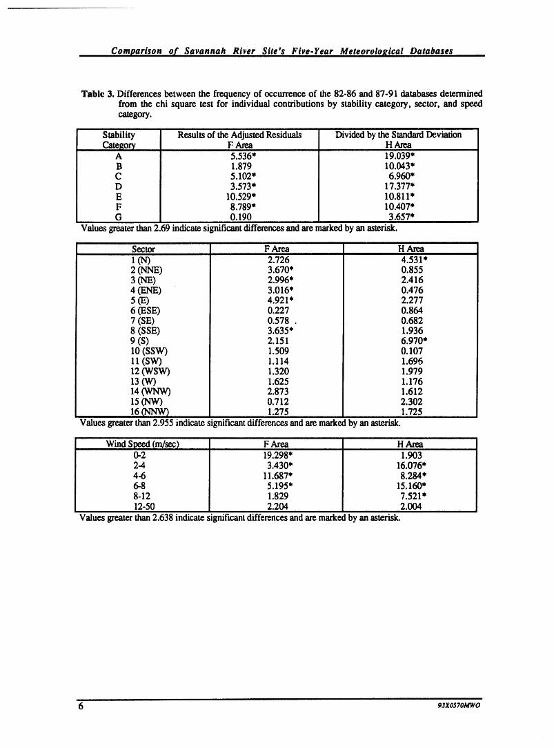
Table 3. Differences between the frequencyof occurrenceof the 82-86 and 87-91 databases determinedfrom the chi square test for individual contributions by stability category, sector, and speedcategory.
Stability Results of the AdjustedResiduals Dividedby the Standard--Deviation,Category F Area H Area
A 5.536* 19.039'B 1.879 10.043"C 5.102" 6.960*D 3.573* 17.377'E 10.529" 10.811"F 8.789* 10.407"G 0.190 3.657*
i
Values greaterthan2.69 indicatesignificantdifferencesandaremarkedby an asterisk.i i i
Sector F Area H Area1(N) 2.726 4.531"2 (NNE) 3.670* 0.8553 (NE) 2.996* 2.4164 (ENE) 3.016" 0.4765 (E) 4.921 * 2.2776 (ESE) 0.227 0.8647 (SE) 0.578 . 0.6828 (SSE) 3.635* 1.9369 (S) 2.151 6.970*10 (SSW) 1.509 0.10711 (SW) 1.114 1.696120VSW) 1.320 1.97913 (W) 1.625 1.17614(WNW) 2.873 1.61215 (NW) 0.712 2.30216_V_ 1.275 1.725
Valuesgreaterthan2.955 indicatesignificantdifferencesandaremarkedby an asterisk.
Wind Speed{m/sec) F Area H Arm0-2 19.298" 1.9032-4 3.430* 16.076"4-6 11.687" 8.284*6-8 5.195' 15.160"8-12 1.829 7.521"12-50 2.204 2.004
Values greater than 2.638 indicate significant differences and are markedby an asterisk.
6 93XO570MWO
, Comparison of Savannah River Site's Five-Year Meteorological Databases
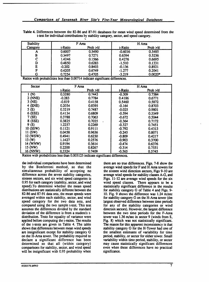
Table 4. Differences between the 82-86 and 87-91 databases for mean wind speed determinedfrom thet-testfor individualcontributionsby stabilitycategory, sector,andspeed category.
Stability F Area H AreaCategory t-Ratio Prob >ltl t-Ratio Prob >ltli
A 0.6007 0.5490 -0.6016 0.5485B 0.3497 0.7271 0.6394 0.5236C 1.4246 0.1566 0.4276 0.6695D 0.4850 0.6283 -1.510 0.1331E -0.202 0.8403 -0.136 0.8921F 0.4205 0.6749 - 1.277 0.2041G 0.7254 0.4705 -3.219 0.0020"
'" i i
Ratios with probabilitiesless than 0.00714 indicate,significantdifferences., ,,
Sector F Area H Areat-Ratio Prob >ltl t-Ratio Prob >ltl
..... i (N) 0.3280 0.7443 -0.309 0.75842 (NNE) .0.283 0.7784 0.4186 0.67713 (NE) .0.819 0.4158 0.5460 0.58724 (ENE) 0.2034 0.8395 -0.164 0.87035 (E) 0.3219 0.7487 .0.025 0.98016 (ESE) 0.4134 0,6809 -0.594 0.55497 (SE) 0.3788 0.7063 .0.672 0.50448 (SSE) 0.3825 0.7035 . -0.364 0.71729 (S) )..2257 0.2269 -0.327 0.7451
10 (SSW) 0.1121 0.9111 .0.792 0.431311 (SW) 0.0458 0.9636 .0.245 0.807112 (WSW) 0.4941 0.6230 .0.809 0.421713 (W) 1.1427 0.2576 .0.903 0.370014(WNW) 0.9194 0.3614 -0.474 0.637615 (NW) 0.2200 0.8267 -0.314 0.755116 (NNW) 0.3324 0.7409 .0.565 0.5745
i
Ratios withprobabilitiesless than 0.003125 indicate significant differences.
the individualcomparisonshavebeendetermined there areno truedifferences. Figs. 7-8 show theby the Bonferroni method, so that the averagewind speeds forF andH Area towersforsimultaneous probability of accepting no the sixteen wind direction sectors, Figs 9-10 aredifference across the seven stability categories, average windspeeds forstability classes A-G, andsixteen sectors, and six wind speed categories is Figs. 11-12 are average wind speeds for the six0.95 foreach category (stability, sector,andwind wind speed classes. There appears to be aspeed).To determine whether the mean speed statistically significant difference in the resultsdistributionsarestatistically differentbetween the for stability category G of Table 4 and Figs. 9-82-86 and 87-91 data sets, the mean speedswere 10. Fig. 9 shows the difference was 1.24 m/secaveraged within each stability, sector, and wind for stabilitycategory G on the H-Areatower (thespeed category for the two data sets, and largest observeddifferencebetween time periodscomparedusing the two _mple t-test.This test for any of the stability categories or windassumes the differences divided by the standard directionsectors).However, the largestdifferencedeviation of the difference is from a student'st- between the two time periods for the F-Areadistribution.Tests for equality of variance were tower was 1.36 m/sec in sector9 (winds fromS,appliedbefore computing the t-ratios. The results Fig. 8) which was not statistically significant.
the t-tests are given in Table 4. The table The reasonfor this apparentinconsistency is thatshows thatdifferences betweenmeanwind speeds stabilitycategory G for the H-Towerhad one ofare insignificant except for stability category G the smallest estimates of variability for time
the H-Areatower. The probabilityrequiredto period,stability, or sectorfor either tower. Smalldeclare a significant difference has been variabilitywithin timeperiod, stability,or sectordetermined so that all (within category) may cause statistically significant differencescomparisonsforstability, sector, and wind speed even when these differences have no practicalwill be insignificant with 0.95 probabilitywhen significance.
i
9JXO570.MWO 7
Comparison oi"Savannah River Site'sFive.YearMeteorologicalDatabases
Sources of Differences Between the 1982-86 and the 1987-91 Databases
(a) Climatic variation
Meteorologicaldatacould be expectedto vary the absolutevalues was 13.2%, a considerablebetween two contiguous five year periods due to amounLThe amountof this shift from Exhibit 1worldwide climatic variations which are caused for the F-Area tower, summed similarlyover theby increased concentrations of optically active stabilitycategories, is equal to 7.92%.constituentsin the atmosphere.The timescale ofthese variations is generally quite long, but A numberof books andpapershave been writtenvariations can occur on shorter time scales, on the connection between climatic variationsMeasuredchanges in the mean temperature for and sunspots, solar flares, and other solarthe Southeast region of the U.S. show a mean activity. Some of the relationships have beentemperature increaseof about 0.6° C from 1982 shown to be statistically significant, but oftento 1991 (Michaels, et al. 1991). A temperature the effect is obscured by other equally importantchange of this amount might be large enough to changes in atmospheric constituents. Sunspotscause changes in the wind frequencydistribution occur over a period of 10-12 yearsand the 82-86and/ormean values, and 87-91 databases are about half the required
period, so sunspot effects on the database,Itis worth noting thatthe statistically significant although slight, mightalso appearin the data.differences in stability categories in Table 3might be a result of the mean temperature 'Climatic variations can also be caused byincrease. Fig. 3 shows a shift between 82-86 and significant atmosphericforcing functionssuch as87-91 from the more stable categories E-G to volcanic activity, El Niflo, deforestation, etc.;more unstable categories A-C, which could be these phenomenonarewell documented.Randomattributedto the temperatureincrease. This shift statistical fluctuations can also occur in anyin stability categories is also found in F-Area turbulentfluid such as the atmosphere. Severaltower data shown in Fig. 4, Exhibit 4 was used causes for statistical differences between the twoto sum the absolute values of the percentage databases exist if we acknowledge thesedifferences over stability categoriesA-C and E-G mechanismsforclimatic variations.for the H-Area tower during 87-91. The sum of
(b) Instrument and coding faults
D. M. Hamby (1992) used the 82-86 and 87-91 Area towers prior to the end of 1987; there isH-Areadata sets in dosimetrycodes to determine also a bivane resolver gap of about one degreethe relative two-hour and annual average x/Q width which occurs at 359.50-0.5° (north)with(concentrationsdivided by sourcestrength) from improvedwind directioninstrumentationinstalledboth data sets. One of Hamby's plots showed a on theArea towersat the end of 1987.noticeabledip for one wind directionsector in anotherwise smooth curve. Examining the curve The algebraicsign faultexcluded wind directionsclosely showed the 87.91 dataset hada relative within the range0 to +5° foran interval of timeminimum in 7JQ for northwinds, after a software maintenance modification was
implemented.The code faultwas carefully tracedAn extensive investigation led to two possible using computer archive tapes and was found tocauses for the north wind minimum have originatedon February24, 1989. The faultconcentrations which have been identified since was corrected on July 29, 1992. Data for 34 ofHamby'sreport:(1) the algebraic sign in an "IF" 60 months of the 87-91 database were affected.
' statement of an archiving module of VAX-8550 The percentage of missing data caused by thissoftware was found to have a positive value factor can be estimated by assuming the windwhere a negative value was required; (2) there is a directions are uniformly distributed.A five degreebivane potentiometer gap of about 3-5° width exclusion zone would havecaused the deletion ofwhich occurs at (north) v,ith bivanes used on the 1.11%of the azimuths in the north sector in the
i i,i1|1
8 9JxoJ7oMwo
, Comparison of Savannah RiverSite'sFive.YearMeteorologicalDatabases
1987-91 databasefor the H-Area tower. It should component translatingmechanical displacementbe noted that the effect of the excluded wind into electrical signals.)Replacement of the olderdirections would actually be spreadsomewhatto bivanes was also highly desirable since it led toadjoining sectors because of turbulent more accurateand reliable wind directions overfluctuationsduringa fifteen minute period, the compass range 359.50-0.5.
' The north wind direction was one of two sectors The effect of the potentiometer gap operatingwhich showed statistically significant differences over a 60 month period for the 1982-86 &_tabase
I in frequency of occurrence and is flagged inTable can be estimated by assumingthe wind directions' 3. The dip in Hamby's _Q curve is caused by are uniformly distributed. A 3-50gap would haveI the wind speeds being biased to lower values caused 0.83-1.39% of the azimuth data around1 and/or the percentage frequency of occurrence north to be missing. For the 12 months in 19871 being lower for the 87-91 data. Both effects are includedin the new database(1987-91), a totalof1 present and can be verified in the tables and 0,17.0.28% of the data would have been affected.i figures. One can determine from Table 4 and theI software used that the negative t-ratio means the The effect of the resolver gap can be estimated1 mean speeds for 4-6 m/see category are biased similarly. If the resolver gap is one degree wideI toward lower values in the 87-91 H-Area and the wind directions are distributeduniformly,1 database. Fig. 1 shows the percentage frequency then about 0.22% of the total azimuths would( of occurrence for North winds is lower for the have been affected in a 48 month period. Wind1 new database for H-Area. tunnel experiments have shown the effect on the
voltage signal caused by the resolver gap is aThe blvanes used prior to the end of 1987 had spurious voltage, i.e., the wind is indicated astwo-potentiometer systems designed to correct . coming from an incorrect sector. This means thatthe problem of bivanes with a single a secondary effect of the reso_ver gap ispotentiometer. The two-potentiometer system excessively large standard deviations of azimuthalways has a wiper in contact with potentiometer angle. This would produce a slightly larger thanwindings and thus generates a valid signal even expected frequency of A-D stability categorieswhen one of the potentiometer wipers is in the when winds blow from the north sector. Thegap. In spite of the existence of the two percentage of data affected is estimated to be thepotentiometer system, it was apparently not same as the percentage of azimuths affectedused, because of complexity of the software that (0.22%).would have been needed. Rather, the system wasoperated with a single potentiometer. This caused The potentiometer andresolver gap effects arenota gap of 3-5* in the wind directions about north independent of the software "sign" omission,prior to the end of 1987. Improved wind because of overlapping azimuth ranges.instrumentswere installed on the Area towers at Consequendy, subjective estimations of the exactthe end of 1987. (Resolvers replaced amount ofdataaffectedinthe 1987-91 databasepotentiometers as the mechanical-electronic have ahigh uncertainty.
I (c) Sources used for filling missing data
1 Data were filled in for the H-Area tower 87-91 0.92% of the wind data for the 87-91 H-Areadatabaseas described earlier. Linear interpolation, tower were substituted from the Plant Vogtledata from backup computers at the towers, and tower.data from nearby Area towers were the preferredchoices for fill-in data. Data from the Augusta The wind instruments used by Plant Vogtle were
1 National Weather Service (NWS) tower and Plant less sensitive than those used on SRS's AreaVogtle were also used when absolutely necessary, towers. The Pasquill-Gifford stability categories
' The NWS service tower was needed for only determined from these instruments utilizedI 0.54% of 1988's wind data or 0.11% of the total fifteen-minute averages of turbulence intensityt five years. The Plant Vogtle tower instruments during the one-hour period rather than true one-
are mounted at 60 meters, about the same height hour averages which include the effect of wind1 as the 61-meter Area tower instruments. Only meandering (as is done at the SRS).
,i
9JxosTo_nvo 9
Comparison of Savannah River Site'sFive.YearMaeoroloRical,Databases,
Providing a Basis for Future Comparisons
(a) Spectra for the 86-91 Database
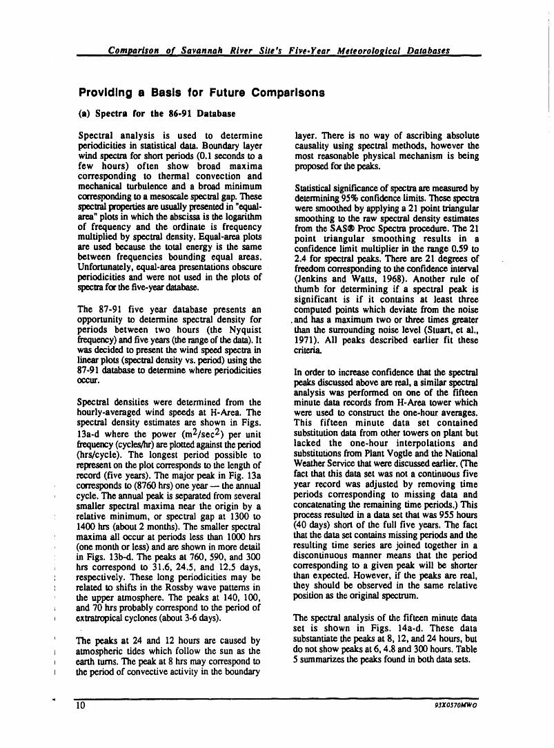
Spectral analysis is used to determine layer. There is no way of ascribing absoluteperiodicities in statisticaldata.Boundarylayer causalityusing spectralmethods,howeverthewindspectrafor shortperiods(0.1 secondsto a mostreasonablephysicalmechanismis beingfew hours) often show broad maxima proposedforthepeaks.corresponding to thermal convection andmechanical turbulence and a broad minimum Statisticalsignificance of spectraaremeasuredbycorrespondingto a mesoscale spectralgap. These determining95% confidence limits. These spectraspectralpropertiesareusuallypresentedin "equal- were smoothed by applyinga 21 pointtriangulararea"plots in which the abscissa is the logarithm smoothing to the raw spectral density estimatesof frequency and the ordinate is frequency from the SAS® Proc Spectraprocedure.The 21multiplied by spectral density. Equal-area plots point triangular smoothing results in aare used because the total energy is the same confidence limit multiplier in the range 0.59 tobetween frequencies bounding equal areas. 2.4 for spectral peaks. There are 21 degrees ofUnfortunately,equal-area presentationsobscure freedomcorrespondingto the confidence intervalperiodicities and were not used in the plots of (Jenkins and Watts, 1968). Another rule ofspectraforthefive-yeardatabase, thumb for determining if a spectral peak is
significant is if it contains at least threeThe 87-91 five year database presents an computed points which deviate from the noiseopportunity to determine spectral density for , and has a maximum two or three times greaterperiods between two hours (the Nyquist than the surroundingnoise level (Stuart,et al.,frequency)andfive years(the rangeof thedam).It 1971). All peaks described earlier fit thesewas decided to present the wind speed spectra in criteria.linear plots (spectraldensity vs. period)using the87-91 database to determine where periodicities In orderto increase confidence thatthe spectraloccur, peaks discussed above arereal, a similarspectral
analysis was performed on one of the fifteenSpectral densities were determined from the minute data records from H-Area tower whichhourly-averaged wind speeds at H-Area. The were used to construct the one.hour averages.spectral density estimates are shown in Figs. This fifteen minute data set contained13a-d where the power (m2/sec 2) per unit substitution data from other towers on plant butfrequency(cycles/hr)areplottedagainstthe period lacked the one-hour interpolations and(hrs/cycle). The longest period possible to substitutionsfrom PlantVogtle and the Nationalrepresenton the plot correspondsto the lengthof WeatherService thatwere discussedearlier.(Therecord (five years). The majorpeak in Fig. 13a fact that this data set was not a continuous fivecorrespondsto (8760 hrs) one year-- the annual year record was adjusted by removing timecycle. The annual peak is separatedfromseveral periods corresponding to missing data andsmaller spectral maxima near the origin by a concatenating the remaining time periods.) Thisrelative minimum, or spectral gap at 1300 to process resulted in a data set that was 955 hours1400 hrs (about2 months). The smaller spectral (40 days) short of the full five years. The factmaxima all occur at periods less than 1000 hrs thatthe data set contains missing periods and the(one month or less) and areshown in more detail resulting time series are joined together in ain Figs. 13b-d. The peaks at 760, 590, and 300 discontinuous manner means that the periodhrs correspond to 31.6, 24.5, and 12.5 days, corresponding to a given peak will be shorterrespectively. These long periodicities may be than expected. However, if the peaks are real,related to shifts in the Rossby wave patterns in they should be observed in the same relativethe upperatmosphere.The peaksat 140, 100, positionas theoriginalspectrum.and70 hrsprobablycorrespondto the periodofextratropical cyclones (about3-6 days). The spectral analysis of the fifteen minute data
set is shown in Figs. 14a-d. These dataThe peaks at 24 and 12 hours are caused by substantiatethe peaks at 8, 12, and 24 hours, butatmospheric tides which follow the sun as the do notshow peaks at 6, 4.8 and 300 hours. Tableearth turns.The peak at 8 hrs may correspond to 5 summarizesthe peaks found in both data sets.theperiod of convective activity in the boundary
l0 ojxo57ol_rwo
Comparison o,fSavannah River Site'sFive.YearMeteorologicalDatabases
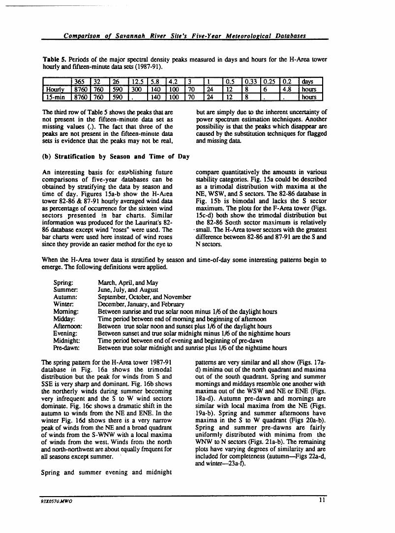
Table 5. Periods of the major spectral density peaks measured in days and hours for the H-Area towerhourly and fifteen-minute data sets (1987-91).
365 32 26 12.5 5.8 4.2 3 1 0.5 0.33 0.25 0.2 da_
Hourly 8760 760 590 300 140 100 70 24 12 8 6 4.8 hours15-rain 8760 760 590 . 140 100 70 24 12 8 . . hours
The third row of Table 5 shows the peaks that are but are simply due to the inherent uncertainty ofnot present in the fifteen-minute data set as power spectrum estimation techniques. Anothermissing values (.). The fact that three of the possibility is that the peaks which disappear arepeaks are not present in the fifteen-minute data caused by the substitution techniques for flaggedsets is evidence that the peaks may not be real, and missing data.
(b) Stratification by Season and Time of Day
An interesting basis for es_blishing future compare quantitatively the amounts in variouscomparisons of five-year databases can be stability categories. Fig. 15a could be describedobtained by stratifying the data by season and as a trimodal distribution with maxima at thetime of day. Figures 15a-b show the H-Area NE, WSW, and S sectors. The 82-86 database intower 82-86 & 87-91 hourly averaged wind data Fig. 15b is bimodal and lacks the S sectoras percentage of occurrence for the sixteen wind maximum. The plots for the F-Area tower (Figs.sectors presented in bar charts. Similar 15c-d) both show the trimodal distribution butinformation was produced for the Laurinat's 82- the 82-86 South sector maximum is relatively86 database except wind "roses" were used. The . small. The H-Area tower sectors with the greatestbar charts were used here instead of wind roses difference between 82-86 and 87-91 are the S andsince they providean easier method for the eye to N sectors.
When the H-Area tower data is stratified by season and time-of-day some interesting patterns begin toemerge. The following definitionswere applied.
Spring: March, April, and MaySummer:. June, July, and AugustAutumn: September, October, and NovemberWinter: December,January, and FebruaryMorning: Between sunrise and true solar noon minus 1/6of the daylight hoursMidday: Time period between end of morning and beginning of afternoonAfternoon: Between true solar noon and sunset plus 1/6 of the daylight hoursEvening: Between sunset and true solar midnight minus 1/6 of the nighttime hoursMidnight: Time period between end of evening and beginningof pre-dawnPredawn: Between true solar midnight and sunrise plus 1/6of the nighttime hours
The spring pattern for the H-Area tower 1987-91 patterns are very similar and all show (Figs. 17a-database in Fig. 16a shows the trimodal d) minima out of the north quadrant and maximadistribution but the peak for winds from S and out of the south quadrant. Spring and summerSSE is very sharp and dominant. Fig. 16b shows morningsand middays resemble one another withthe northerly winds during summer becoming maxima out of the WSW and NE or ENE (Figs.very infrequent and the S to W wind sectors 18a-d). Autumn pre-dawn and mornings aredominate. Fig. 16c shows a dramatic shift in the similar with local maxima from the NE (Figs.autumn to winds from the NE and ENE. In the 19a-b). Spring and summer afternoons havewinter Fig. 16d shows there is a very narrow maxima in the S to W quadrant (Figs 20a-b).peak of winds from the NE and a broad quadrant Spring and summer pre-dawns are fairlyof winds from the S-WNW with a local maxima uniformly distributed with minima from theof winds from the west. Winds from the north WNW to N sectors (Figs. 21a-b). The remainingand north-northwest are about equally frequent for plots have varying degrees of similarity and areall seasons except summer, included for completeness (autumn--Figs 22a-d,
and winter--23a-f).
Spring and summer evening and midnight
93xo57oa_wo 11
Comparison of Savannah River Site's Five-Year Meteorological Databases ,,
Conclusions
New procedures and meteorological instruments differences between the new and old data sets.resulted in a significant gain in the percentageof Only the G stability category for H-Area towervalid datacapturedin annualdatasets forming a indicateda significantdifferenceoutof the sevenbasis for the 198%91 database.The datarecovery stabilitycategories and sixteen direction sectors.percentage for the last four years of the 87-91 This difference was only 1.24 m/see for the Gdatabase was well above 90%. The missing and stability class. This gives a measure ofbad data decreasedby a factor of three from the confidence that dosimetry calculations will not1982-86 database. This fact and the considerable change significantly when using the 87-91 datawork expended in filling in missing periods for set.the new database permitteddetailed analyses thatcould not have been performed on the earlier The fact that the two data sets have differentdatabase, mean wind speed distributionsfor theG stability
class may be due to the fact that the 82-86The chi-squarestatisticwas used to compare the database was created using an outlier screeningfrequencyof occurrencefor two time periods for test. This could have eliminatedvalid dataduringF-Area and H-Area towers. The chi-square frontal passages, thunderstorms, periods of lightstatisticshowed therewere significantdifferences winds, etc., when there were valid reasons toby stability, wind direction sector, and wind expect a given Area tower to show a differentspeedclass. The chi-squarestatisticdoes not have . wind direction than the others. If these cases ofthe ability to show wherethe differences exist, so screening out valid data was not uniformlythe standardizedadjustedresidual together with distributed,thena bias could have beenc_ inthe Bonferronimethod was used. These methods the mean wind speeds (or frequency ofshowed that only two of sixteen wind direction occurrence).It would seem reasonableto assumesectors (north and south) had statistical that application of the Dixon ratio test duringadifferencesbetween the 82-86 and87-91 datasets period of light winds (nighttime, stablefor the H-Area tower. Reasons were found to conditions)probablyresultedin morecases beingexplain the northsector difference but the south rejectedfor the 82-86 database.sectorremainsunexplained. The differences in thenorth wind sector were probably due to a The statistical tests used to detect differencescombination of a coding faultand the instrument between the two data sets is quite sensitivemaker's design for the wind direction because of the large number of observationsinstruments. The F-Area tower showed five available.A summaryof the ability of statisticalsectors with differences but these may reflect a tests to determinedifferencesis as follows:combinationof naturalmeteorologicalvariabilityand differences in the methods used to createthe • Largesamplesizes providethe abilitydatabases" to detectsmalldifferencesbetween
categories.Tests on the differencebetween the two data sets • Small variabilityin meanwind speedsusing the standardizedadjustedresidual together providesthe ability to detect smallwith the Bonferroni method showed that a differencesbetweencategories.majority of stability categories and wind speed • Small sample sizes only provide theclasses weredifferent forboth F-AreaandH-Area abilityto detectlargedifferencestowers. The reasons for the differences in betweencategories.stability categories may be related to an increase • Largevariabilityin meanwindof 0.6° C in temperatureover the ten yearperiod, only providesthe ability to detectClimatic variations resulting from volcanic largedifferencesbetweencategories.activity, El Niflo, and deforestation could causedifferences both in stabilitycategories and speed Power spectrashow expected peaks at periods ofclassesbetween the datasets. one yeardue to the earth'srotationabout the sun,
3-6 days due to extratropicalcyclones, 24 and 12hours due to solar tides. The probable cause is
The majority of mean wind speeddifferences for not apparentforpeaks occurringat periods of 32-both H-Area and F-Area towers when examined 26 days and8 hours.by sector, and stability category showed no
12 93X057oaiwo

.- Comparison of Savannah River Site's Five-Year Meteorological Databases
B Bar charts were used to compare the distribution Spring and summer evening and midnightol of stability categories within wind direction patterns are very similar and all show minimas4 sectors. The frequency distribution by wind out of the north quadrant and maxima out of thedJ direction sector could be described as a trimodal south quadrant. Spring and summer mornings anddJ distribution with maxima at the NE, WSW, and middays resemble one another with maxima outS S sectors, of the WSW and NE or ENE. Autumn pre-dawn
and mornings are similar with local maxima
When the H-Area tower data is stratified by from the NE. Spring and summer afternoons ares¢ season and time-of-day some interesting patterns similar with maxima in the S to W quadrant.el emerge. The spring pattern shows a trimodal During spring and summer pre-dawn winds are
distribution with dominant winds from the S and fairly uniformly distributed with minima fromS; SSE. Northerly winds become very infrequent the WNW to N sectors.dl during summer and the south through west windsd_ dominate. In the autumn a dramatic shift occurs The new 87-91 H-Tower data set provides a goodtc to winds from the NE and ENE. In the winter basis for future comparisons since the additional
there is a very narrow peak of winds from the NE time and effort spent on quality assuranceal and a broad quadrant of winds from the S to provides more confidence that new information
WNW with a local maxima from the west. determined by inference and by statisticalWinds from the N and NNW are about equally methods is valid.
fr frequent for all seasons except summer.
m
9J 93xoszoawo 13
Comparison of Savannah River Site's Five.Year Meteorolo[_ical Databases
References
Dixon, W. J., and F. J. Massey, Jr., 1957: Michaels, P. J., 1991: Frosts and Freezes,Introduction to Statistical Analysis, 2nd Ed., Southeastern Climate Review, ISSN 1050-1428,McGraw-Hill, New York, pp. 275-278, and 412. Vol. 2/No. 4, Spring 1991. Southeast Regional
Climate Center, 1201 Main St. Columbia, SC
Hamby, D. M. ,1992: Atmospheric Transport 29201.31 pp.Modeling Utilizing Meteorological Data setsgenerated by Two Quality Assurance Methods. Parker, M. J., R. P. Addis, C. H. Hunter, R. J.Inter-Office Memorandum, SRT-ETS-920191. Kurzeja, C. P. Tatum, and A. H. Weber, 1992:Westinghouse Savannah River Company, Aiken, The 1987-1991 Savannah River SiteS.C. Meteorological Database (U). WSRC-RP-598.
Westinghouse Savannah River Company, Aiken,
Jenkins, (3. M. and D. G. Watts, 1968: Spectral S.C.Analysis and Its Applications. Holden-Day, 525pp. Stuart, W. F., Sherwood, V. and Macintosh, S.
M., 1971: The power spectral density technique
Laurinat, J. E., 1987: Average Wind Statistics applied to micropulsation analysis. Pure Appi.for SRP Area Meteorological Towers. DPST-87- Geophys., 92, pp 150-164.341. Savannah River Laboratory, E. I. DuPont,Aiken, S. C.
Comparison of Savannah River Site's Five.Year Meteorological Databases ,
Appendix A
Statistical Calculations
Statisticaltestswereperformedto testthefollowinghypothesis,termedthenullhypothesis:
Ha: Therearcno differencesbetweenthe distributionsin the old andnew datasets.
Differences were determinedin the numberof observations for eachof seven stabilitycategories, 16 winddirection sectors, and six wir.d speed categories by comparing the number observed with the numberexpectedm_ingthechi-squaredistribution.
Dcf'mitionof terms:
Let nij = numberof actualobservationsfor data set i (i=l for the 87-91 data set andi=2 for the 82-86data set) and class j, (j=l to 7 for stability categories,j=l to 6 for wind speed categories, andj=l to 16 forwind directionsectors.)
Ni+ = _nij = total numberobservations for data set i summedover all classes (j=l to 7 forstabilitycategories,j=l to 6 forwind _ categories,andj=l to 16 forwind directionsectors.)
N+j = gn U= total numberof observations in categoryj summed overboth data sets.
N = N1 + N2 = _N+j = totalnumberof observations in both data sets.
Under thenull hypothesis, the same proportionin each category shouldcome fromeach data seLThus, if pjis theproportionobserved in category-j overboth datasets, then the same proportionof each data set shouldalso be in category-j or
pj = N+j/N.
The expected numberof observationsin each class is given by
Fij =pj * Ni+ =Ni+ * N+j/N.
The squared difference between the observed and expected numberdivided by the expected numberofobservations is termed the adjusted residual squared.The adjusted residual squared is summed over allcategoriesfor bothdata sets.
rij2 = (nij- Fij)2/Fij, and
X2 = g,_.,rij2.
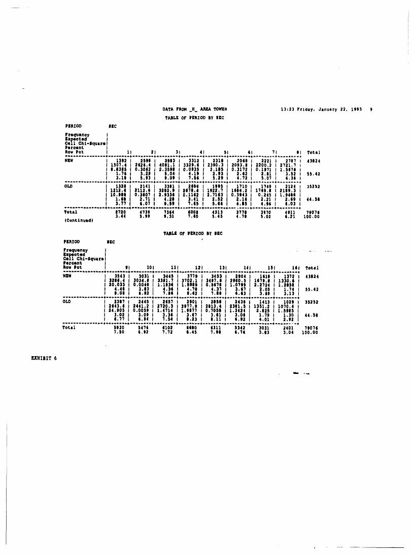
presented in Exhibit 1 for stability category andThe _2 ratio is distributed asa chi square random F-Tower data, Exhibit 2 for wind speed categoryvariablewith (I-1)0-1) degrees of freedomwhere I and F-Tower data, Exhibit 3 for wind direction= 2 and J = no. of categories, 6, 7 or 16. Since sectors for F-Tower data, Exhibit 4 for stabilitythere are only two data sets, the number of category and H-Tower data, Exhibit 5 for winddegrees of freedom is equal to the number of speed category and H-Tower data, Exhibit 6 forcategories minus one. wind direction sectors and H-Tower data. In
addition to the _2 defined above, two additionalSAS@ (Proc Freq) software was used to analyze chi-square variables are computed by [email protected] data. The results of the SAS® procedure are These are the likelihood ratio _2 and the Mantel-
93xo57o._veo 15
, Comparison of Savannah River Site'sFive.YearMeteorologicalDatabases
Haenszel Chi-Square.Probabilities of accepting periods for the jth category. The simultaneousthe null hypothesis based on these two additional probabilityof accepting all J comparisons whentests were approximatelythe same as for the chi- the null hypothesis is true was set to be 0.95squaretest discussed. These additionaltests will (95%confidence of accepting the null hypothesisnot be described. SAS® (Proc Freq)also when it is true.) In order to have thecomputes three tests forassociation between the simultaneous probability equal to 0.95, theclasses and the time periods. These are the Phi individualcomparisonprobabilitiesof acceptanceCoefficient, Contingency Coefficient, and were determinedusing the following BonferroniCramer'sV. Since no probabilitiesof acceptance method.nor rejection arecomputed, these were not usedandarenotdescribed. 0_2 ffi(1-0.95)/(72).
A frequency table is also included with the two For the seven stability categories, o,/2 ffi0.0036time periods (NEW for 87-91 data set and OLD and z(1-a/2) = 2.69. For the six wind speedfor 82-86 data set) as the two rows, and stability, categories, or/2 = 0.0042 and z(1-ot/'2) = 2.638.sector, or wind speed category as the column. For the sixteen sectors, a/'2 = 0.00156 andThe numbersin eachcell are labeled underperiod, z(1-cff2) = 2.955.The first value is the number observed, the
second is the number expected under the null Additionalstatistical tests were performedfor thehypothesis, the third is the cell chi-square null hypothesis that there is no difference in thecontribution or the adjusted residual squared mean wind speeds between the two data sets. To(rij2), the fourth is the percent of the total of test this null hypothesis, an analysis of varianceboth data sets in the cell and the last numberis (ANOVA) was done which modeled the meanthe percent of each data set in the cell. The .wind speedas a function of time period, stabilitymarginal totals for the rows include the total per category, and wind direction sector. The meanrow or data set and the percentof the total in each wind speedwas determinedfromthe originaldatadata set. The marginal totals for columns gives by grouping all the observations into 672the total per column or category and the percent categories (seven stability by six wind speed byof the total in each category which is the 16 sectors) and calculating the average windexpectedproportionunderthe null hypothesis, speed. These 672 meanwind speeds were the set
of observations analyzed by the analysis ofSAS® Proc Freq does not compute the adjusted variance.The wind speed class was not includedresidual divided by its standarddeviation. The in the model since there is a correlationbetweenresidual squaredis computed and labeled as the mean wind speed and wind speed category. Thecell chi-squarevalue. The standarddeviation(Sij) model also included the two-factor interactionsof theadjustedresidualis given by which are the interactionbetween time periods
and category and between stability and sectorcategories. The results aregiven in Exhibit 7 for
I Sij--"[(1-N+j/N)(1-Ni+/N)] 1/2. F Tower and Exhibit 8 for H Tower. Onlystability was a significant factor in the analysis
' The random variable, eij = rij/Sij, is distributed of variance.i approximately as a normal variate with mean1 zero and variance one. Since only two time An analysis of variance was also done withI periods are being compared, elj = - e2j for all j stability as a blocking factor (this compares onlyI categories. Thus, residuals need to be computed the differences between time periods within eachI foronly one data set anda two-tailed comparison stability category and not the averages betweenI basedon the normal distributionis made. stability category). When this was done, there
was no significant difference between timeI Since each individualcomparisonis distributedas periods. If there are significant differencesI a normal (0,1) variate, the probabilityof getting between time periods, the F-test on the period
a larger absolute value can be determined by within stability factor will be inflated and theI Prob{leijl< z(l-cx/2)} = (l-a) if the null probability of getting a larger F-value will bet hypothesis is true where z(1-a/2) is the small. This was not the case when both period1 100(1-_r2) percentile for the normaldistribution, within stability category and period within sector
category were compared.The F-test is similar to
1 Thus, if the calculated leijl ._z(l-o_f2),accept the the chi-square in that it only indicates significantI null hypothesis of no difference between time differences acrossall subeategories butnot which
subcategory(ies) are different. The results for
i 16 9_XO_7OMWO
, Comparison of Savannah Rive r $1tels Five.Year MeteoroloMcal Databases
differences between data sets within stability either anequal or unequalvariance t-test.SAS®category for F-Tower data is shown in Exhibit 9 ANOVA proceduredoes not test for equality ofand for sector in Exhibit 10. The results for variances. For these reasons, the two sample t-stability category for H-Tower data is shown in testswere used.Exhibit 11 and for sectors in Exhibit 12 for H-
Tower. SAS ® procedure"VI'ESTwas usedto computethe t-test or t.ratio between the two time periods
The 672 mean wind speeds for each time period foreach of the 7 stability categories, and 16 windwere averaged for each of the seven stability directioncategories. The mean windspeeds werecategories, sixteen sectors, and six wind speed averaged within each time period. TTESTcalegories within each time periodand compareA calculates the average, variance, standardusinga two samplet-test. There is one difference deviation,F-ratio, probabilityof getting a largerbetweenthe two sample t.test done separatelyfor F-ratio,t-ratio,and probabilityof getting a largereach category and the ANOVA. In the ANOVA Itl ratio assuming both equal and unequalthe variance estimates within time periods and variances. The ratio of the largest variance tocategories are pooled, while in the t-test, a smallest variance is compared with thepreliminaryF-test is done to determineif the true correspondingpercentilesof the F-distributionsovariances between time periods within each that two-tailed percentiles are used (folded Fcategory can be consideredequal, and depending statirtic).on the results of the F-test, SAS® computes
Let xijk = the kth meanwind speed for timeperiod i in categoryj, then
iij .= Y.Xijk/nijand
sij2 = E(Xijk - iij. )2/(nij- 1),
Then for each category -j, form the following ratio
F = largest of Slj 2 and s2j2/smallest of Slj2 and s2j2.
The probability computed by SAS® is a the probability of getting a larger ratio under theassumption
t_lj2 =o2j2.
The two sample t-test is given by
t= (Xlj.-i2j.)/Sdj
Ifthevariancesareassumedtobcequal,thenthestandarddeviationofthedifferenceinaveragewindspee,dsisgivenby
Sdj= Spj(I/nlj+ I/n2j)If2with(nlj+ n2j-2)degreesoffreedom.
Spj2= [(nlj.l)Slj2+ (n2j-l)s2j2]/(nlj+n2j-2).
Ifthevariancesarcassumedtobcunequal,thenthestandarddeviationofthedifferenceisgivenby
Sdj= [(Slj2/nlj)+ (s2j2/n2j)]If2.
Thedegreesoffreedomaregii,enby(Satterwaite'sapproximation)
dfj= {[(Slj2/nlj)+(s2j2/n2j)]}/{[slj4/(nlj-l)]+ [s2j4/(n2j-l)]}.
93xosTo_wo 17
Compa_',_vonof Savannah RDer Slte'sFlve.YearMeteorotoRlcaIDatabases
Again the probabilityof simultaneousacceptance However, SAS has already computed theof all J comparisonswhen the null hypothesis is probability that Itl > t(1-cx/2)(dfj) or Prob.true was set at 0.95 and the probability of {Itl>t(l-¢x/2)(dfj)} = a. So the Bonferroniaccepting each individual comparison was adjustmentfor a for the SAS two-sample t-testsdewrmined using the Bonferroni method. Each is given byindividual t-ratio is distributedas a student's t-
distributionwithdfj degrees of freedom.Thus, if ¢x= (1-0.95)/J.t(1-a/2)(dfj) is the 100(1-_'2) percentile of thestudent's t-distribution with dfj degrees of For the 7 stability categories ¢x= 0.00714. Forfreedom, then Prob.{Itl_ t(l.ct/2)(dfj)} = (1 - ¢x), the sixteen wind directions, cz = 0.003125 andwhere dfj is the degrees of freedom for the jth ¢x= 0.00833 for the six wind speedcategories.category. The Bonferronimethod requiressolvingthe following for ¢x Results from the SAS® TTEST procedure are
shown in Exhibits 13, 14, and 15 for stability,¢Z/2= (1-0.95)/(2"J). sector, and wind speed, respectively for the
F-Tower data and in Exhibits 16, 17, and 18respectively,for the H-Towerdata.
m
18 _Jxo57ouwo
Comparison of Savannah RiverSite'sFlve.YearMeteorologicalDatabases
References for Appendix A:
SAS@ User's Guide: Version 6.03, SAS® Satterwaite. F. W., 1946: "An ApproximateInstituteInc. Box 8000, Cary, N C. Distribution of Estimates of Variance
Components,"Biometrics Bulletin, 2, 110-114.Reynolds, H. T., 1977: The Analysis of Cross-Classifications, TheFree Press,N'Y. Miller, R. G., Jr., 1981: Simultaneous
Statistical Inference, Springer-Verlag,NY.
93XO570J_fWO

,, Comparison of Savannah RiverSite'sFlve.YearMeteorologicalDatabases ,
T/u'spageintentionally left blank
20 ....................... 9,xo.o_.;O

_. , Comparison of"Savannah R!v.frSite'sFive.Year'MeteoroloRlcalDo,tabases,
AppendiX B .................... ...................
Ap AppendixB containsa numberofplots forF and H.Areatowersforboth the 82-86 & 87-91 datasets whichare are too numerousto commenton individuallywithin thetext, nevertheless,occasions will arise when theseplo plots areneededforvariouspurposes.Theirbreakdownis as follows:
(1) (1) plots showinghow the stabilitycategoriesaredistributedover the speed classes (Figs. 24a-d)
(2) (2) plots showing how thespeedclasses aredistributedoverthe stability categories(Figs. 25a-d)
O) O) plots showinghow the speedclasses aredistributedoverthe directionsectors(Figs. 26a-d)
(4) (4) plots showing how the directionsectorsaredistributedover the stabilitycategories (Figs. 27a-d)
9Jxo 9Jxo_7oJ,_wo 21

, comp,a,r!sonof 5avannob River Site'S Five.Year MeteorolomtcalDatabases ,-
Thispageintentionallyleftblan_
22 _ " ,_xos_o_o
.... Comparison,of,,Sa,vannahRiverSite'sFive.YearMe,te,oroloRlcal£)atabases ,,
Exhibits
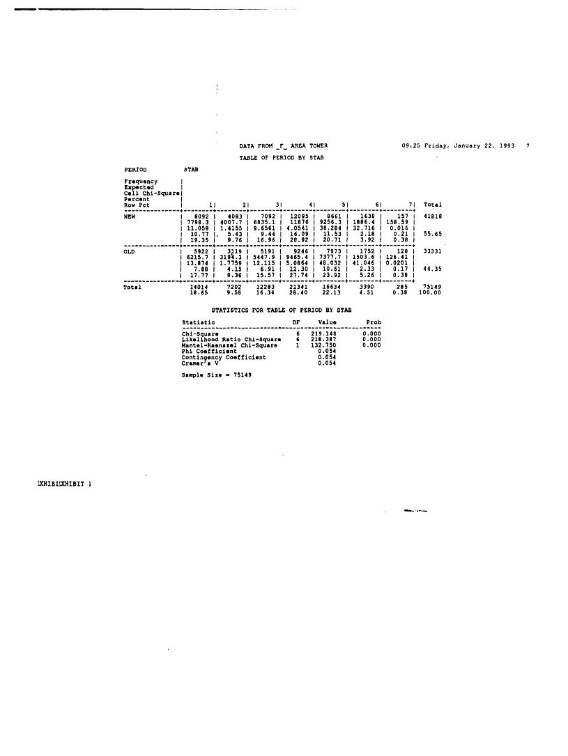
Exhibit 1. Tables from SAS® Proc Frequency for F.Area Tower. Comparisonof New versus Old databasesby the seven stabilityclasses, "New" r_fersto 1987-91 data,"Old" is 1982.86 data.
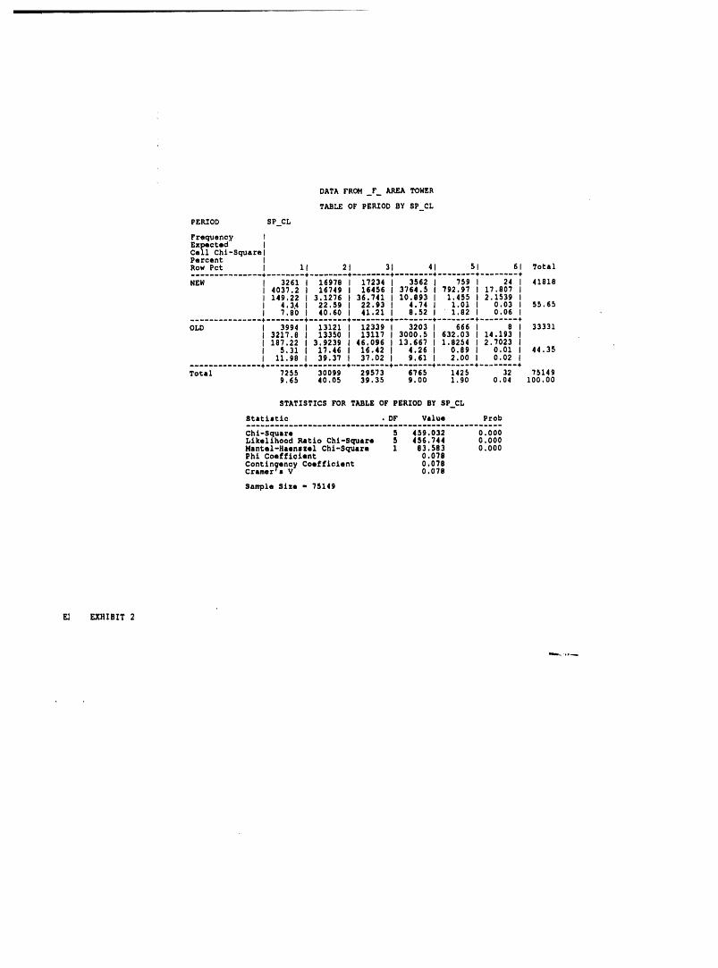
Exhibit2. As in Exhibit I except forcomparisonsby the six windspeed classes.
Exhibit 3, As in Exhibit 1 except forcomparisonsby the sixteen sectors,
Exhibit4, As in Exhibit 1 except for H-Areatower,
Exhibit5, As in Exhibit I except forH-Areatowerandcomparisonsby the six wind speed classes.
Exhibit6. As in Exhibit 1except for H-Areatower andcomparisonsby the sixteen sectors,
Exhibit 7. Tables fromSAS® Pro(:GLM(GeneralLinearModels) for the average speed from the F-Areatower, "STAB" refers to the seven stability classes, "SEC" refers to the sixteen sectors, and"PERIOD" refersto thetwo datasets,
Exhibit8. As in Exhibit 7 except for the H.Area tower.
Exhibit9, As in Exhibit 7 except thatthe two datasets"PERIOD" aremodeled as nested within the sevenstability"STAB" classes,
Exhibit 10, As in Exhibit 9 except for the two data.setsare modeled as nested within the sixteen sectors"SEC".
Exhibit 11, As in Exhibit 9 except for the H-Area tower,
Exhibit 12, As in Exhibit 10except for the H-Areatower,
Exhibit 13, Tables fromSAS@ Proc 'I'TESTforcomparing theaverage wind speed from the F.Area rowerbetween the twodatasets,"NEW" versus"OLD" within each of the seven stabilityclasses.
Exhibit 14. As in Exhibit 13except forcomparisons within each of the sixteen sectors.
Exhibit 15. As in Exhibit 13 except forcomparisonswithin each of the six wind speed classes.
Exhibit 16. As in Exhibit 13except for H.Area tower.
Exhibit 17. As in Exhibit 14 except for H.Area tower.
Exhibit 18, As in Exhibit 15 except for H.Area tower,
_ __m
9_xo_7oJ#_'o 23

......,Comoarlsonof Savannah River Site'sFive.year MeteoroloRlcal'Data#a,s,es,,,
Thispageintentionallyleftblank
2_ 93xoJ70MWO
Comparison of Savannah River Site's Five.Year Meteorological Databases
Figures
Figure 1. Percentage of H-Area tower Figure 13a. Spectral density estimates of one-observations from the 82-86 (solid) and 87-91 hour mean wind speeds for the 87-91 H-Area(dashed)databasesforeachwinddirectionsector towerdatabase.Spectraldensityestimateshave(1-16). units of power (m2/sec 2) per unit frequency
(cycles/hr) and are plotted against the periodFigure 2. Percentage of F-Area tower (hrs/cycle).observations from the 82-86 (solid) and 87-91(dashed)databases foreach wind directionsector Figure 13b. Same as Fig. 13a except for a(1-16). limitedrangeof theperiod.
Figure 3. Percentage of H-Area tower Figure 13c. Same as Fig. 13b except for aobservations from the 82-86 (solid) and 87-91 limitedrangeof theperiod.(dashed) databases for each stability class(A-G). Figure 13d. Same as Fig. 13c except for a
limitedrangeof the period.Figure 4. Percentage of F-Area towerobservations from the 82-86 (solid) and 87-91 Figure 14a. Spectral density estimates of fifteen-(dashed) databases for each stability class minute mean wind speeds for the 87-91 H-Area(A-G). towerdatabase.Spectral densityestimateshave
units of power (m2/sec2) per unit frequencyFigure 5. Percentage of H-Area tower • (cycles/hr)and arc plottedagainstthe periodobservationsfrom the 82-86 (solid) and87-91 (his/cycle).(dashed)databasesforeachwindspeedclass (O-
2- >12). Figure 14b. Same as Fig. 14a except for alimited range of the period.
Figure 6. Percentage of F-Area towerobservations from the 82-86 (solid) and 87-91
Figure 14c. Same as Fig. 14b except for a(dashed)databas_ foreach windspeedclass (0-2 -- _12). limitedrangeof the period.
Figure 7. Mean wind speeds for the H-Area Figure 14d. Same as Fig. 14c except for atower from the 82-86 (solid) and 87-91 (dashed) limitedrangeof theperiod.databasesforeach winddirectionsector (1-16).
Figure 15a. Percentage of H-Area towerobservationsfrom the 87-91 databases for each
Figure8. Mean wind_ for the F-Areatowerwind direction sector (1-15) broken down byfrom the 82-86 (solid) and 87-91 (dashed)
databasesfor each winddirectionsector (1-16). stabilityclass.
Figure9. Meanwind _ for the H-Areatower Figure 15b. As for 15aexcept for82-86.from the 82-86 (solid) and 87-91 (dashed)databasesforeach stabilityclass (A-F & G). Figure 15c. As for 15a except for the F-Area
tower.
Figure 10. Mean wind speeds for the F-Areatower from the 82-86 (solid) and 87-91 (dashed) Figure150. As for 15c except for82-86.da_ -basesfor each stability class (A-F & G).
Figure 16a. Frequencyof occurrence of H-AreaFigure 11. Mean wind speeds for the H-Area towerobservations from the 87-91 databases fortower from the 82-86 (solid) and 87-91 (dashed) each wind directionsector (1-16) brokendown bydatabasesfor eachwindspeedclass(1-6), stability class for the spring season (March,
April, May).
Figure 12. Mean wind speeds for the F-Areatower from the 82-86 (solid) and 87-91 (dashed) Figure 16b.As for 16aexcept for summer(June,databasesforeachwind_ class (I-6). July, August).
93xo57o._wo 25
Comparison of Savannah River Site's Five.Year Meteorological Databases
Figure 16c. As for 16a except for autumn Figure 22b. As for 17a except for autumn and(September,October,November. evening.
Figure 16d. As for 16a except for winter Figure 22c. As for 17a except for autumn and(l_ember, January,February). afternoon.
Figure 17a. As for 16a except for evening Figure 22d. As for 17a except for autumn and(between sunset and true solar midnight minus midday.1/6 of the nighttimehours).
Figure 23a. As for 17a except for winter andFigure 17"o.As for 17aexcept for midnight(time morning.periodbetween end of evening and beginning ofp_-dawn). Figure 23b. As for 17a except for winter and
midday.Figure 17c. As for 17a except for summerandevening. Figure 23c. As for 17a except for winter and
afternoon.Figure 17d. As for 1To except for summerandmidnight. Figure 23d. As for 17a except for winter and
evening., , Figure 18a. As for 17a except for spring and
morning (between sunrise and true solar noon Figure 23e. As for 17a except for winter andminus 1/6 of the daylighthours). .midnight.
Figure 18b. As for 17a except for spring and Figure23t".As for 17aexcept for winterand pre-midday (time period betweenend of morningand dawn.beginning of afternoon).
Figure 24a. Percentage of H-Area towerFigure 18(:.As for 17a except for summer and observations from the 87-91 database for eachmorning, speed class (0-2 m >12) broken down by
stabilityclass (A -- F-G).Figure 18d. As for 17a except for summer andmidday. Figure24b. Same as Fig. 24a except for 82-86.
Figure 19a. As for 17a except for autumn and Figure 24c. Same as Fig. 24a except for the F-pre-dawn (between sunrise and true solar Areatower.midnight plus 1/6 of the nighttimehours).
Figure 24d. Same as Fig. 24c except for82-86.Figure 19b. As for 17a except for autumnand
morning. Figure 25a. Percentage of H-Area towerobservations from the 87-91 database for each
Figure 20a. As for 17a except for spring and stabilityclass (A -- F-G) broken down by speedafternoon (between sunset and true solar noon class (0-2 -- >12).plus 1/6 of the daylight hours).
Figure25b. Same as 25a except for 82-86.Figure 20b. As for 17a except for summer and
afternoon. Figure 25c. Same as 25a except for the F-Areatower.
Figure21a. As for 17aexcept forspringand pre-
dawn. Figure 25d. Same as 25c except for82-86.
Figure 2lb. As for 17a except for summer and Figure 26a. Percentage of H-Area towerpie.dawn, observations from the 87-91 database for each
direction sector (S -- SSE) broken down byFigure 22a. As for 17a except for autumn and speed class (0-2- >-12).midnight.
26 9Jxo.f70Mwo
.. Comparison of Savannah River Site's Five.Year Meteorological Databases ,
E Figure26b. Same as Fig. 26a except for82-86.
Ft Figure 26c. Same as Fig. 26a except for theF, F-Are,a tower.
Ft Figure 26d. Same as Fig. 26c except for82-86.
FJ Figure 27a. Percentage of H-Area towerol observations from the 87-91 database for eachst stability category (A-G) broken down by sector(S (S -- SSE).
Ft Figure 27b. Same as 27a except for 82-86.
Ft Figure 27c. Same as 27a except for the F-Areatower.
Fl Figure27d. Same as 27c except for 82-86.
,, , Comparison of Savannah River Site'sFive.Year MeteorologicalDatabases ,
This page intentionally left blank
93XOJTOMWO
DATA FROM _f AREA TOWER 09:25 Friday, January 22, 1993 7
TABLE OF PERIOD BY STAB
PERIOD STAB
Frequency JExpected lCell Chi-SquarelPercent IRow Pct l iI 21 31 41 51 61 71 Total............... +........ +........ +........ +........ +........ +........ +........ +
NEW l 8092 l 4083 1 7092 l 12095 1 8661 1 1638 I 157 1 41818J 7798.3 j 4007.7 J 6835.1 j 11876 j 9256.3 J 1886.4 J 158.59 JI 11.058 I 1.4155 I 9.6561 J 4.0541 I 38.284 I 32.716 I 0.016 ll 10.77 J, 5.43 I 9.44 J 16.09 1 11.53 I 2.18 I 0.21 I 55.65I 19.35 I 9.76 I 16.96 I 28.92 I 20.71 1 3.92 I 0.38 I
............... +........ +........ +........ +........ +........ + ........ + ........ +
OLD J 5922 j 3_19 j 5191 J 9246 I 7973 J 1752 I 128 I 33331I 6215.7 I 319_.3 I 5447.9 I 9465.4 l 7377.7 I 1503.6 i 126.41 jI 13.874 l 1.7759 I 12.115 l 5.0864 I 48.032 l 41.046 I 0.0201 II 7.88 j 4.15 I 6.91 I 12.30 I 10.61 I 2.33 I 0.17 j 44.35I 17.77 I 9.36 I 15.57 I 27.74 I 23.92 I 5.26 I 0.38 I
............... +........ +........ +........ +........ +........ +........ +........ +Total 14014 7202 12283 21341 16634 3390 285 75149
10.65 9.58 16.34 20.40 22.13 4.51 0,38 100.00
STATISTICS FOR TABLE OF PERIOD BY STAB
Statistic DF Value Prob__...__._.___._. .......... 6.... ......... ... ....... ....
Chi-Square 6 219.148 0.000Likellhood Ratio Chi-Square 6 218.387 0.000Mantel-Haenazel Chi-Square 1 132.750 0.000Phi Coefficient 0.054
Contingency Coefficient 0.054Cramer'8 V 0.054
Sample Size - 75149
_XHIBI_XHIBIT 1
DATA FROH_F_ AR/_A TOWER
TABLE OF PERIOD BY SP_CL
PERIOD SP CL
Frequency TExpected ICell Chl-SquarelPercent IRow Pct l II 21 31 41 5l 61 TotAl
+ + + + . . +
NEW J 3261 j 16978 J 17234 J 3562 I 759 J 24 j 41818I 4037,2 j 16749 I 16456 I 3764.5 I 792,97 I 17.807 lI 149,22 I 3,1276 J 36,741 J 10.893 i 1,455 i 2.1539 il 4.3_ I 22.59 I 22,93 I 4.74 I 1.01 I 0,03 I 55.65l 7,80 I 40,60 I 41,21 I 8,52 I 1,82 I 0,06 I+ + + + + + +
OLD ! 3994 i 13121 I 12339 I 3203 I 666 I 8 I 33331) 3217.8 I 13350 I 13117 I 3000°5 I 632,03 I 14,193 II 187.22 I 3.9239 I 46,096 I 13,667 I 1,8254 I 2,7023 II 5.31 I 17,46 I 16.42 I 4.26 I 0.89 i 0,01 I 44.35I 11.98 I 39.37 I 37.02 I 9.61 I 2,00 I 0.02 I
.... ..... ....................--...............--..................+ + + + . + .TotAl 7255 30099 29573 6765 1425 32 75149
9,65 40.05 39.35 9,00 1,90 0,04 i00,00
STATISTICS FOR TABLE OF PERIOD BY SP CL
StatlmClc • DF VAlue Prob
Chi-SquAre 5 459.032 0.000Likelihood Ratio Chi-SqruAre 5 456.744 0.000Mantel-Haenszel Chl-SquAre 1 83.583 0,000Phi Coefflolent 0,078Contingency Coefficient 0,078CrAmer'a V 0,078
Sample SiZe - 75149
EXHIBIT 2
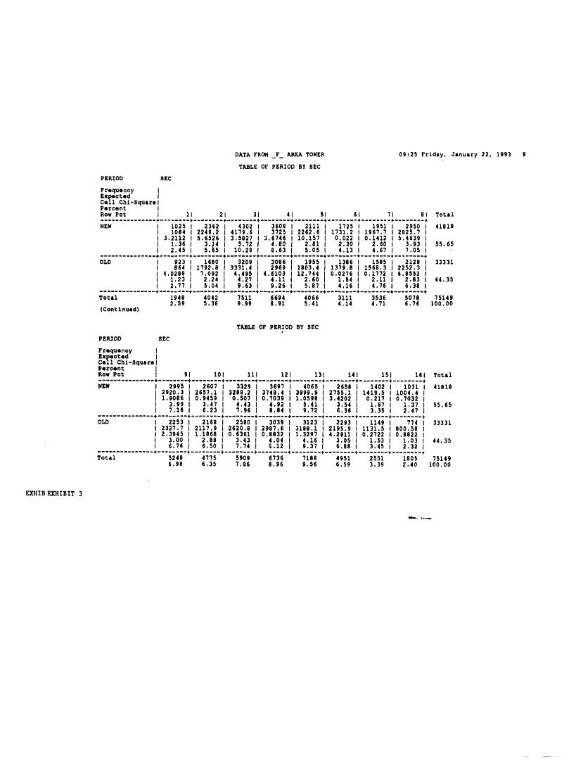
DATA FROM _F_ _,qY_ATOWER 09:25 Friday, January 22, 1993 9
TABLE OF PERIOD BY $EC
PERIOD SEC
Frequency IExpected iCell Chi-Square IPercent iRow Pet I 11 21 3f 41 51 61 71 81 Total............... +........ +........ +........ +........ +........ +........ +........ +........ +NEW I 1025 I 2362 1 4302 1 3608 1 2111 1 1725 1 1951 1 2950 1 41818
) 1084 i 2249.2 0 4179.6 I 3725 I 2262.6 I 1731.2 I 1967.7 I 2825.7 1i 3,2112I 5.6526i 3.5827i 3,6746i 10.157I 0.02210.1412i 5.4639It 1.36I 3,_4 I 5.72 I 4.80 I 2.81f 2.301 2.60 _ 3.93 I 55.65I 2.451 5 _5 i 10,29t 8.63 I 5,051 4.131 4.67I 7,05 I
............... + ........ +........ +.... ..... ........ ......... +........ ......... .........O,D , 923, 168oI 3209I 3086, i955, 1386, 1585, 2128, 33331
I 664I 1792.8I 3331.4a 2969_ 18034 i 1379., , 15683 , 2252.3,i 4,0288 1 7.092 I 4.495 I 4.6103 I 12.744 I 0.0276 I 0.1772 I 6.8552 II 1.23 i 2,24 I 4.27 I 4.11 I 2.60 I 1,84 I 2,11 i 2.83 t 44.35I 2.771 5.04 i 9.631 9.261 5.671 4.161 476a 6.38i
............... +........ + ........ +........ +........ ..........+ ........ +........ +........+Total 1948 4042 7511 6694 4066 3111 3536 5078 75149
2.59 5.38 9,99 8.91 5.41 4.14 4.71 6.76 100.00(Cont i nued )
TABLE OF PERIOD BY $EC4
PERIOD BEC
Frequency IExpected lCell Chi-Square I
Percent ]Row Pct 91 101 111 12l 131 141 151 161 Total+ + + + + + . + +
NEW I 2995 I 2607 I 3329 I 3697 I 4065 I 2658 I 1402 I 1031 I 41818I 2920.3 I 2657.1 I 3288.2 I 3748.4 I 3999.9 I 2755.1 I 1419.5 I 1004.4 II 1.9086 I 0.9459 I 0.507 i 0.7039 I 1.0598 I 3,4202 i 0.217 I 0.7032 II 3.99 I 3.47 I 4.43 I 4.92 I 5.41 I 3.54 I 1.87 I 1.37 I 55.65J 7.16 I 6.23 I 7,96 J 8.84 I 9.72 I 6.36 I 3.35 I 2,47 I
............... +.... .... +........ +........ +...... _.+ ........ +.... ....+........ +........ .OLD I 2253 I 2168 I 2580 I 3039 I 3123 I 2293 I 1149 I 774 I 33331
I 2327.7 I 2117.9 I 2620.8 I 2987.6 I 3!88.1 I 2195.9 i 1131.5 I 800.58 iI 2.3945 i 1.1868 I 0.6361 I 0.8832 I 1.3297 I 4.2911 I 0.2722 I 0.8822 II 3.00 I 2.88 I 3.43 I 4.04 I 4.16 I 3.05 I 1.53 I 1.03 I 44.35I 6.76 I 6,50 I 7,74 I ._,12 I 9,37 I 6,88 i 3,45 I 2,32 I+ + + + + + + + +
Total 5248 4775 5909 6736 7188 4951 2551 1805 751496.98 6.35 7.86 8.96 9.56 6.59 3.39 2.40 100.00
EXHIB EXHIBIT 3
DATA FROH_r_ AREA TOHER 09z25 friday, Oanuacy 22, 1993 i0
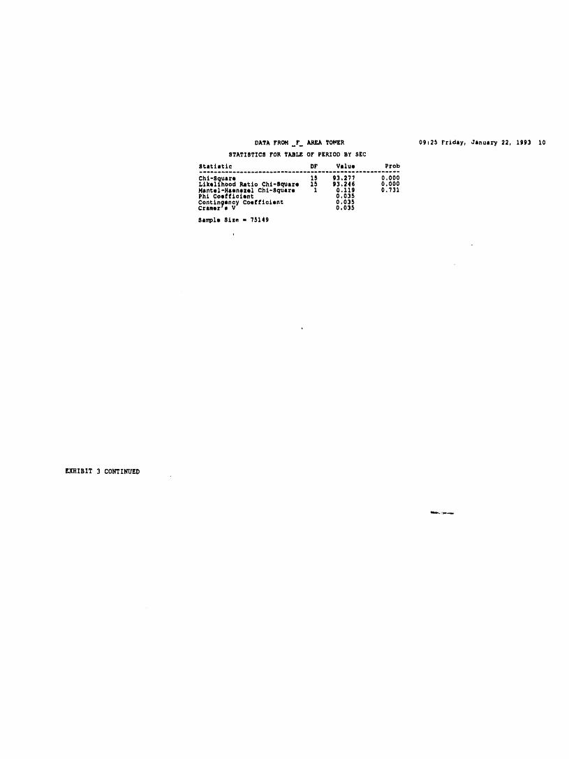
STATISTICS roR TABLE OF PERIOD BY SEC
Statistic DF Value Prob
Chi-Squate 15 93.277 0.000Likelihood Ratio Chi-Square 15 93,246 0.000Hantel*Haenazel Chi-Square 1 0,119 0.731Phi Coeffioient 0.035Conttngenay Coefficient 0.035Cramer'z V 0.035
Sample Size - 75149
EXHIBIT 3 CONTINUED
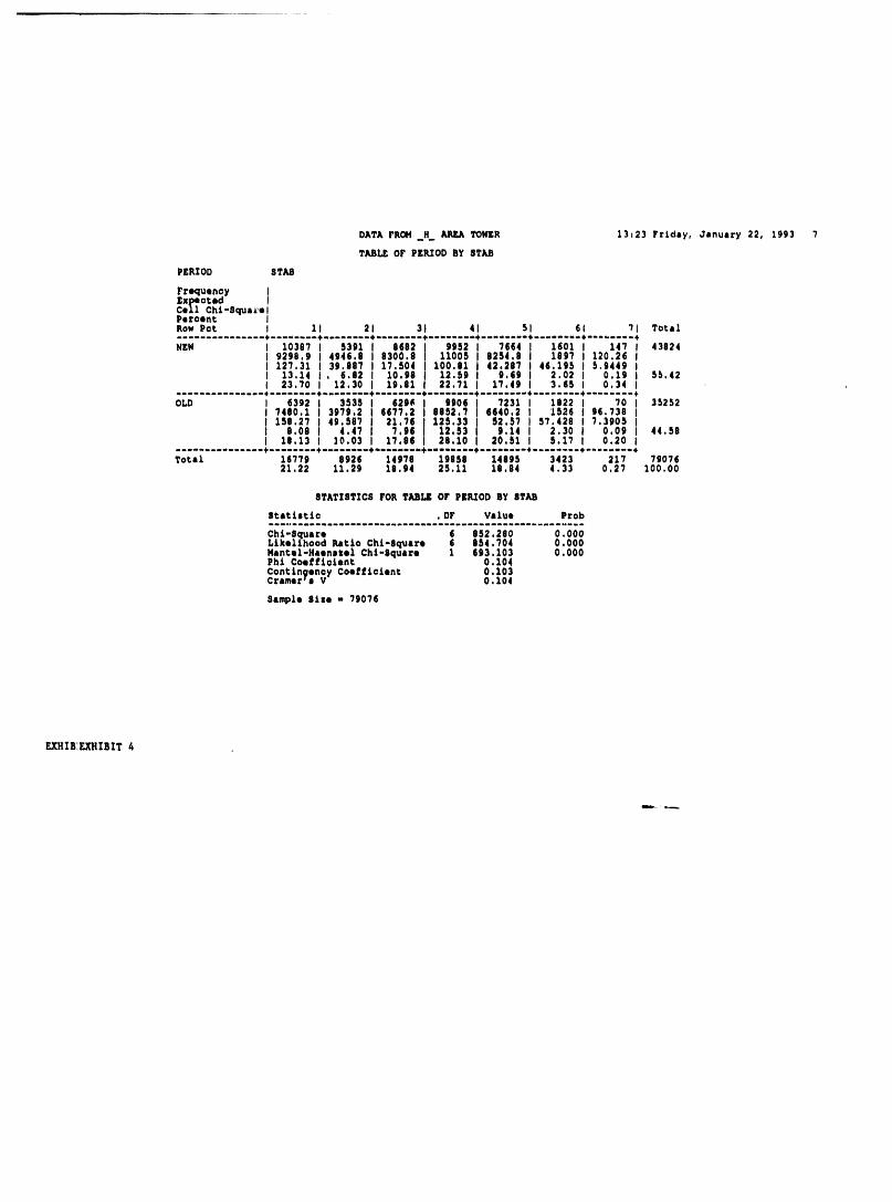
DATA FROH H_ AP_..,ATOWER 13t23 rrlday, January 22, 1993 7
TABIJ_ OF PEI_XOD BY STAB
PEI_OD STAB
rrequenqy_Xpe=ted 1Cell Cht-Squa_elPetoent IRow Pet I 11 21 31 4 51 61 71 Total.... ..... .. .... ,........,........,........, .... ....,........,........,........,
.,. , 1030.I 53., ..°2I 99.2 "41 .01, 147,4,°2,,92.,9 4,.al.oo, 11oo,..0 ..,.0.26,,127.3113,.°°7117.so41-o..,2.287146.1-,s..491, 13.1, , 6.02, 10.9, 12.,9 9., ,.02, o.l,, 55.42, .._0,..30,..,l22.7117.,9,3..,0.34,
............. ..,........,........,........,........,.......-, ........ +.... .... +OLD t 6392 I 3535 i 629_ 9906 7231 I 1822 I 70 I 35252
I 7480.1 I 3979.2 I 6677,2 $852.? 6640.2 I 1526 I 96.738 I
08 I 4,41 96 12,53 9,14 I 2.30 I 0,09 44.58I 18,13 I 10.03 I 17.86 28.10 20.Sl I 5.1_ I 0.20 I
......... .... ..+ ....... .,........,........,........,........,.... .... +.....m._.Total 16779 8926 14978 19858 14695 3423 217 79076
21.22 11.29 18.94 25.11 10.84 4.33 0,27 100,00
STATISTICS FOR TABLE OF PERIOD BY STAB
Statistic . Dr Value Prob
Ch/-Bquare 6 652.280 0.000Likelihood Ratio Chi-Square 6 854.704 0,000Hantel-Haenszel Cht-Square 1 693.103 0.000Phi Coefficient 0.104Contingency Coefficient 0.103Cremer*o V 0.104
Sample Si#e - 79076
EXHIEF.XHIBIT 4
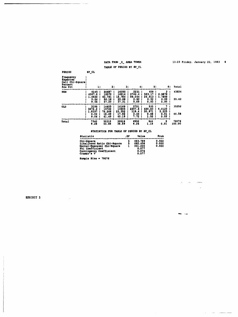
DATAPROHH_ _ YOUR 13t23 friday, JanuJry 22, 1993 8
T_LE or Pr.lLtODBY SPCL
PZMOD SP_CL
rreclueney IExpe©tod IC111 ChL-Square IPercent I_.ov Fat I 11 21 3 41 SI 61 Totalmeese m m eelee em4i_ 4_ i,m+ e. 4mB_ W*qDee_mm4m_l_m_ amsewm m m,_mm _e_ bee+ e amm e mia+m m_ e DN I-- +
HmN I 4145 I 2040? 1|3S0 2231 408 I 2 I 43824
I 4087,8 I 19570 14914 2744,4 523,17 J 4,8870 II 1.4430 83,741 18,794 94.044 24,913 I 1,?$98 II S.2A 26.14 20,68 2.13 0.52 I 0,00 I 55.42I 9.48 I 47.20 37,31 5.09 0.93 I 0,00 I
oLD , 31,si 14e25 141,9 2721, s3s, ? , 3525_, 3272,2, 15742 13,0_ 220?.4, 420.83 , 4.0122 ,, I.,I,7 , 79.286 23.352 119.4, 30.971 , 2.225 ,l 4,04 i 18.4' 17.92 3.44 i 0.48 I 0,01 i 44,59, 9.01, 41.49 40.I0 ?.?_, 1.52 , 0.02 ,
Total 7340 35312 30519 4952 944 9 780769.;18 44.96 38.59 8._4 1.19 0,01 100,00
8TATIIITXC8 for YKBLEor IL)|RXODBY 8P,¢L
StatLoti© , Dr Valuo Ptob
Chi-Sclusre 5 413.799 0,000Likelihood Ratio ¢hL-Ilquire 5 462.456 0.000Hantel-HJenasel Chi-Square 1 331.340 0.000PhL ¢oe_oLent 0.07?¢ont Lngenay Coe_LoLent, 0.074C_er's V 0,077
Ila_ple lise - 7907_
EXHIBIT 5
DA?A r_oH H AN_ _Otfl_R 1]t23 friday, Janumry 22, 19g_ 9
TNIILE or PERZODBY sEc
PERZOD 8EC
r:equeney IExpe©tmd iCl_l Cht-lqul_iPercent IRow Fat I 11 2i 31 41 $1 tl ?t II ?eta1
I .o.3 2.3,,...4 40.. ,3....I 1-00.21 ,21 ,
i 10,100 0.3107 2.135t 0.1112 2.7143 0,3143 I 0.245 I 1.S480 I1.ii 2.11 4,2i 3.4_ _.S2 2.11 I 2,21 I 2,i_ I 44.5iI 3,?? 1,07 I,St ?.iS S,15 4.55 I 4,1| I 4.03 I
TO_Sl 2720 4730 7314 100i 4313 3110 ]S?0 4911 740743,44 S.4t 9,31 7.10 S.45 4,70 5,02 4,21 100.00
(ContLhuid)
?JUILI Or _RZOD BY ||C
F|_ZOD I_c
rrequenuyI_peated I .......Col1 ¢h_-|q_are IPe_aen_ iRow Po_ I 4l 101 111 22l 13l 141 151 111 Tot,!
_0,033 0,004o _,_o3, _.55o_ i o.st?o _,0750 2.2?24 _ _.2o55 _I 4,40 ,34 ?l 4.37) l.O, I 6.3'034, _.ll I :* il' ?.U 1.133'I?j ] 05I.i, I 3.131'74II 5_,42
-.....-I .... ...,........,........,........,........, ..... ...,........,........,........,
O_D i 2307 I 2445 I 2i57 I 2901 I 2|5| 2438 J 1413 I 1024 t 352S2I 2143.1 2441.2 27_0.3 I _977.4 I 2013.4 2351.5 i 1351,_ I 1070.4 t
0,0051 0,70S| 2.3424 54852,4714 2.4177 I I I
$4 4,23 I 0.11 t.52 I 4.01 I 2,t2 ,
To_,l St30 5476 4102 ltlO t311 5342 3031 2401 7907t?.50 6.42 ?,72 1.4S ?.40 4.74 3.03 3,04 100,00
_IBIT 6
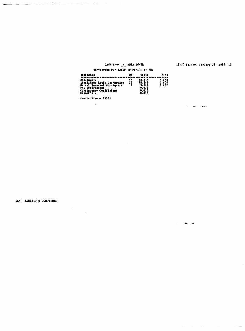
DATAr_ON.H_ AJU_ TO_n 13t2_ rr_d,y. J,,u,ry 22. 199_ 10
ITATZlTZC_ roR TAJIt_ or PEFLTODBY aEC
|tstLItLe Dr Value Prob
Chi-|quateLLkelLhood P.atio Chi-|qusre IS D|.tll 0.000Hantel-Haen||el Chl-|qua:e 1 9,4ai 0.002PhL ¢oeffLeLent 0.055ContLnsmnoyCoeffAoient 0.055Crumr_e V 0.035
|ample 8Lle - ?90?6
I[XH1 I[XHZ|IT 6 COH'rlH_J[D
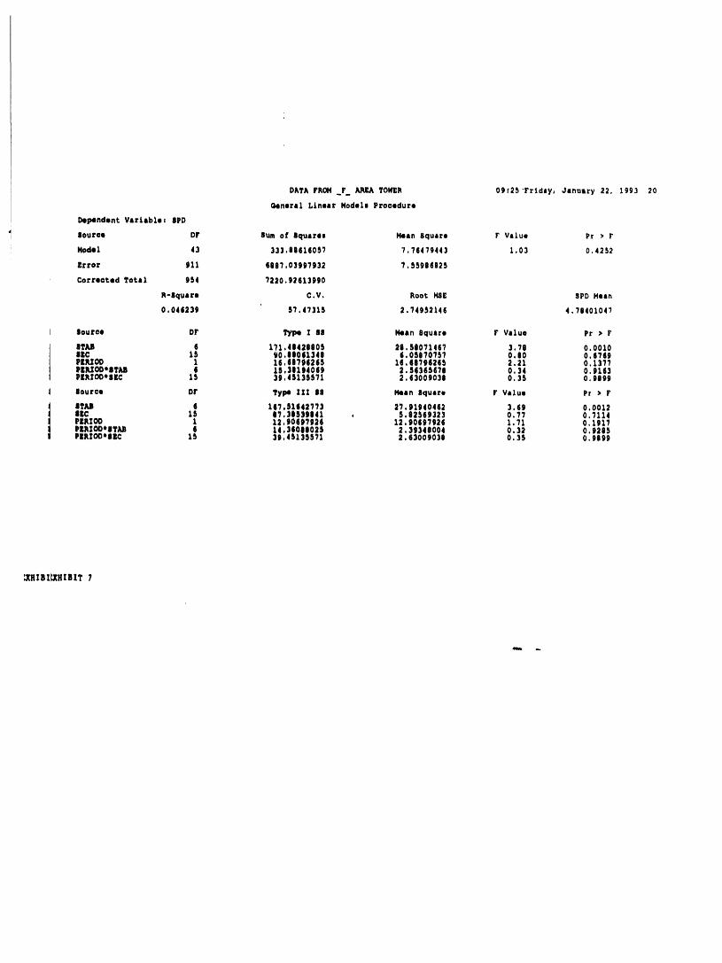
DATArRoH r _ TOWER 09f25"frtdjy, Osnuary 22, 1993 20
QenerI1 Linear Nodal| Prooedure
Dependent Variablet SPD
i huroe Dr Sum of Squares HeIn Squire r Value Fr > r
Node1 43 333,i061(037 7.76479443 1.03 0.4252
_rror 911 6087,0399?932 7.S5986025
Corrected Torsi 9S4 7220,92613990
R-Square C.V. Root HSE SPD Hean
0.046239 57,47316 2.749S2146 4.78401047
$out=e or Type ! BB Neln Squire r Value Pr > r
87NII 6 IT1,4|42580S 28.580714(? 3.78 0.00108|¢ 15 90.110t1348 6.0S870757 0,i0 0.6749PtlIJOD 1 16,4|794245 14.4|?94265 2,21 0.1377PlI_OD*BTAII t 15,]|294069 2.56365678 0.34 0,9243PERZOD*|[C 15 39,45135571 2.43009038 0.3S 0,9899
Source Dr TyPe ZZI Sl Heen |quire r Value Pr • r
8?All i 1i7,51442773 27.91940442 3.69 0.0012l|C 15 07,30539041 . 5,82569323 0.7? 0.7114PERIOD 1 12,t069?1a6 12.90697926 1.?1 0.1917FI_IOD*ITU 6 14.3606|023 2,39348004 0.32 0.9265PlRZOD*IIC 15 30,4S1355?1 2.63009030 0.35 0.9899
_'HIBI_IIBIT 7
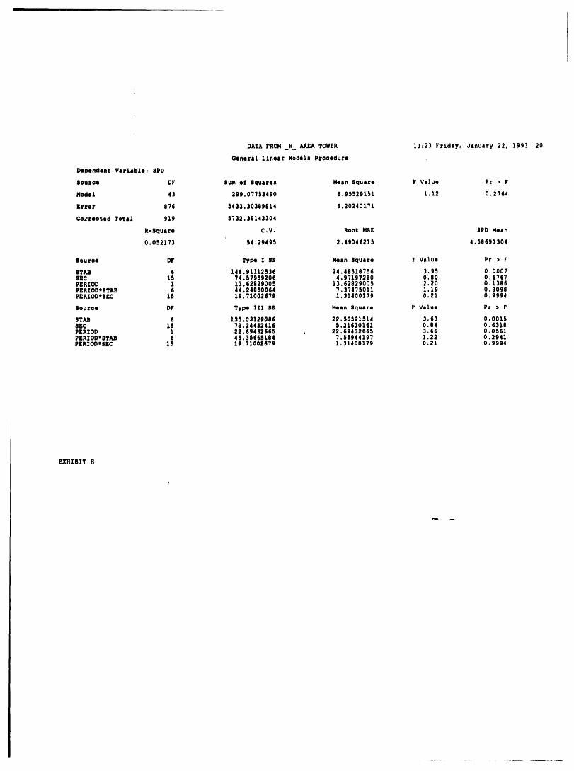
D_?A PROH_H _ ?OHER 13_23 Friday, January 22, 1993 20
General Linear Hodela Procedure
Dependent Variables 8FD
Source DF Sum of Squares Hean Square r Value Pr > F
Node1 43 299.0??53490 6.95329151 1.12 0.2?64
Error 8?6 5433.30389814 6.20240171
Co,rooted Total 919 5732.30143304
R-Square C.V. Root HSE SPD Hean
0.0521?3 54.29495 2.49046215 4.58691304
Source Dr ?ype ! 88 Neon Square F Value Pr > r
8TAIS 6 i44,91112536 24.48518?56 3.95 0.0007SZC i5 ?4.5?959206 4,97197280 0.80 0.6?6?PKRIOD 1 13042|29005 13.62829005 2.20 0.1386PERIOD*ST,_B 6 44,24050064 ?.37475011 1.19 0.3098PERZODeSr_ i5 19,71002679 1,31400179 0,21 0.9994
Source Dr Type iII ES Hean Square P Value Pr > F
STAB 6 135,03129096 22,50521514 3.63 0.00158_C 15 78.24452416 5.21630161 0.84 0.6318PIRZOD 1 22,69432665 , 22.69432665 3.66 0.0561PERZOO*$TAB 6 45.35665184 T.55944197 1.22 0.2941PERZOO*SEC 15 19.71002679 1,31400179 0.21 0.9994
EXRIBIT 8
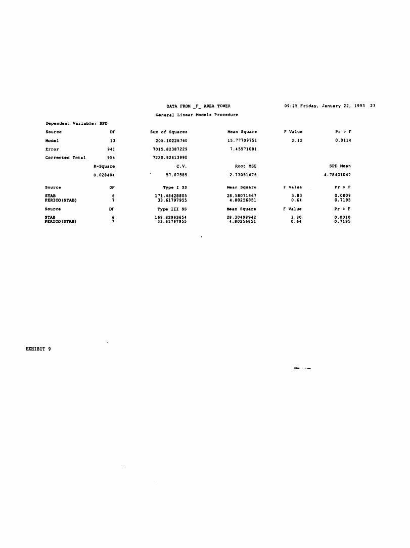
DATA FROH F AREA TOWER 09:25 Friday, January 22, 1993 23-- --
General Linear Hodels Procedure
Dependent Variable: SPD
Source Dr Sum of Squares Hean Square F Value Pr > F
Node1 13 205.10226760 15.77709751 2.12 0.0114
Error 941 7015.82387229 7.45571081
Corrected Total 954 7220.92613990
R-Square C.V. Root MSE SPD Mean
0.028404 57.07585 2.73051475 4.78401047
Source DF Type I SS Hean Square F V#lue Pr > F
STA_ 6 171.48428805 28.58071467 3.83 0.0009PERIOD(STAB) 7 33.61797955 4.80256851 0.64 0.7195
Source DF Type III SS Mean Square F Value Pr • F
STAB 6 169.82993654 28.30498942 3.80 0.0010PERIOD(STAB) 7 33.61797955 4.80256851 0.64 0.7195
EXHIBIT 9
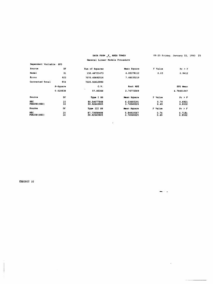
DATA FROH F_ AREA TOWER 09:25 Friday, January 22, 1993 25
General Linear Models Procedure
Dependent Variable : SPD
Source DF Sum of Squares Mean Square F Value Pr > F
Model 31 150. 46721473 4. 85378112 0.63 0. 9412
Error 923 7070,45892516 7. 66030219
Corrected Total 954 7220.92613990
R-Square C.V. Root HSE SPD Mean
0. 020838 57. 85366 2. 76772509 4. 78401047
Source DF T_ I SS Mean Square F Value Pr • F
SEC 15 90.54077868 6.03605191 0.79 0,6921
PERIOD (SEC) 16 59. 92643605 3. 74540225 0.49 0. 9532
Source DF Type III SS Mean Square r Value Pr • F
SEC 15 87. 73658498 5. 84910567 0.76 0.7191PERIOD (SEC) 16 59. 92643605 3. 74540225 0,49 0. 9532
EXHIBIT 10
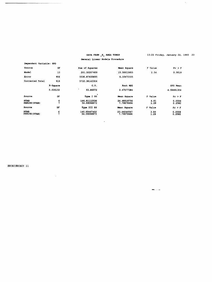
DATA FROH_HAREA TOWER 13:23 Friday, January 22, 1993 23
General Linear Model, Procedure
Dependent Variable: SPD
Source DF Sum of Squares Mean Square F Value Pr > F
Model 13 201.50207409 15.50015955 2.54 0.0019
Error 906 5530.87935895 6.10472335
Corrected Total 919 5732.38143304
R-Square C.V. Root MSE SPD Mean
0.035152 ' 53.86572 2.47077384 4.58691304
qSource DF Type I $S Mean Square F Value PE > F
STAB 6 146.91112536 24.48518756 4.01 0.0006PERIOD(STAB) 7 54.59094873 7.79870696 1.28 0.2582
Source DF Type III SS Mean Square F Value Pr > F
STAB 6 140.65467402 23.44244567 3.84 0.0009PERIOD(STAB) 7 54,59094873 7.79870696 1.28 0.2582
_CHIBILXIIIBIT 11
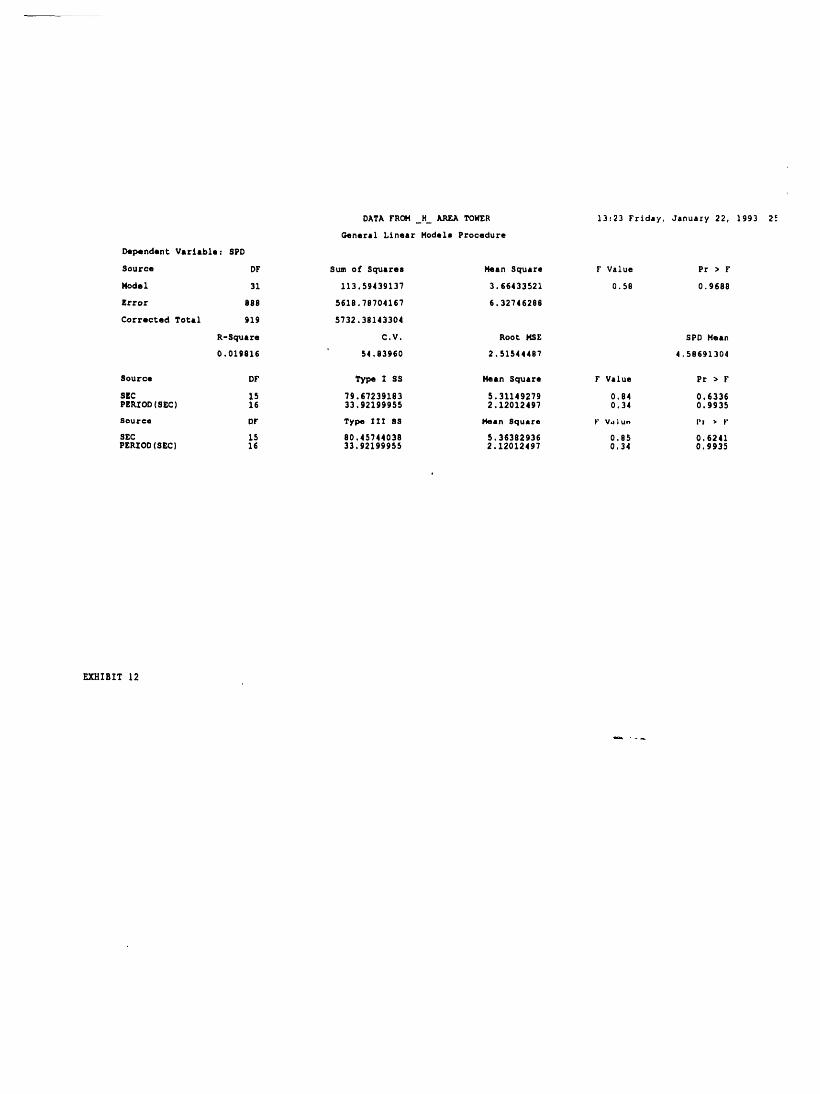
DATA FROM _H_ _ TOWER 13:23 Friday, January 22, 1993 25
General Linear Models Procedure
Dependent Variable: SPD
SoUrce DF Sum o£ Squares Mean Square F Value Pr > F
Model 31 113.59439137 3.66433521 0.58 0.9688
Error 8SB 5618.78704167 6.32746288
Corrected Total 919 5732.38143304
R-Square C.V. Root MSE SPD Mean0
0.019816 54.83960 2.5154448? 4.58691304
Source DF Type I SS Mean Square F Value PE • F
SEC 15 79.67239183 5.31149279 0.84 0.6336PERIOD(SEC) 16 33.92199955 2.12012497 0.34 0.9935
source Dr Type IZI 8S Meen Square V Wlu. t'r > V
SEC 15 80.45744038 5.36382936 0.85 0.6241PERIOD(SEC) 16 33.92199955 2.12012497 0.34 0.9935
EXHIBIT 12
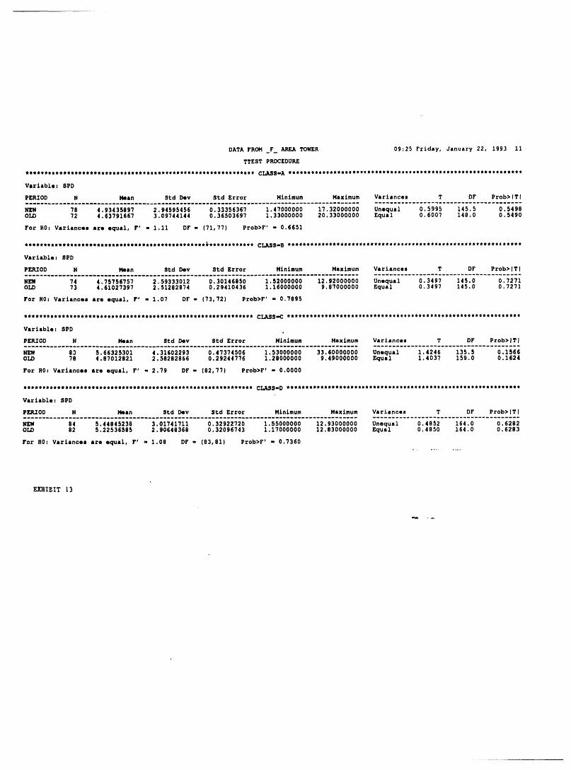
DATA FROH _F_ AREA COWER 09:25 Friday, January 22, 1993 11
TTEST PROCEDURE
*t*e**ttt*_tt**_*t_ttt*_tt_*tt**tttf_tm_t****t_*_ttt*_t*tt_t* CLASSm_ tt**t,_tt_,t,_tItettttt,tt_ttttst**t_*_t_t_,ttttt_tt,ttQ*
Variable: SPD
PERIOD N Mean Std Dev Std Error Minimum Maximum Variances T DF Prob>_Tl
NEW 78 4.93435897 2.94595456 0.33356367 1.47000000 17.32000000 Unequal 0.5995 145.5 0.5498OLD 72 4.63791687 3.09744144 0.36503697 1.33000000 20.33000000 Equal 0.6007 148.0 0.5490
For H0: Variances are equal, F' - I.Ii DF - (71,77) Prob>F' - 0.6651
Variable: SPD
PERIOD N Mean $_d Dev Std Error Minimum Maximum Variances T DF Prob>ITl
NEW 74 4.75756757 2.59333012 0.30146850 1.52000000 12.92000000 Unequal 0.3497 145.0 0.7271OLD 73 4.61027397 2.51282874 0.29410436 1.16000000 9.87000000 Equal 0.3497 145.0 0.7271
For H0: Variances are equal, F' - 1.07 DF - (73,72) Prob>F' - 0.7895
************************************************************* CLASSmC **************************************************************
Varlable: SPD
PERIOD N Mean Std Dev Std Error Mi,imum Maximum Variances T DF Prob>ITl
NEW 83 5.66325301 4.31602293 0.47374506 1.53000000 33.60000000 Unequal 1.4246 135.5 0.1566OLD 78 4.87012821 2.58282866 0.29244776 1.28000000 9.49000000 Equal 1.4037 159.0 0.1624
For H0: Variances are equal, F' - 2.79 DF - (82,77) Prob>F' - 0.0000
Varlable: SPD
PERIOD N Mean Std Dev Std Error Minimum Maximum Variances T DF Prob>ITl
NEW 84 5.44845238 3.01741711 0.32922720 1.55000000 12.93000000 Unequal 0.4852 164.0 0.6282OLD 82 5.22536585 2.90648368 0.32096743 1.17000000 12.83000000 Equal 0.4850 164.0 0.6283
For H0: Variances are equal, F' - 1.08 DF - (83,81) Prob>F' - 0.7360
EXHIBIT 13
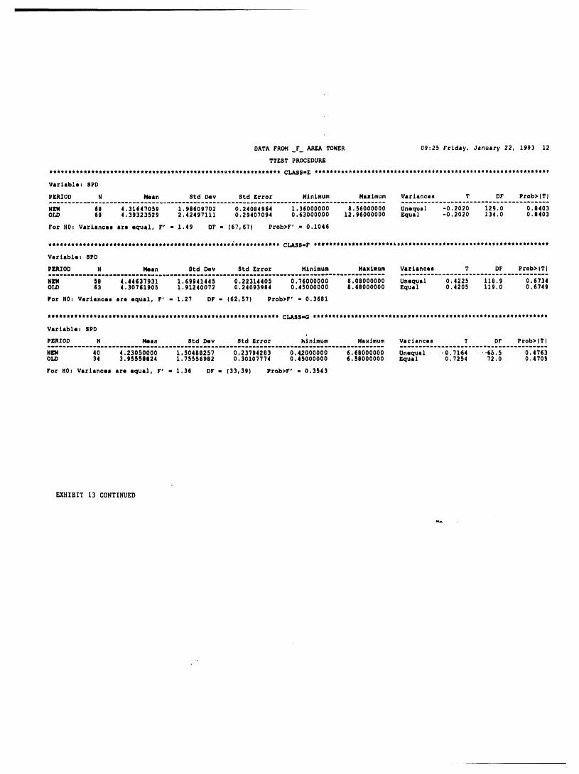
DATA FROM _r_ AREATOWER 09:25 Friday, January 22, 1993 12
TTEST PROCEDURE
#Qtttt#tt#t#Qt#ttt#t#ttttt*t*tt#t##t####R#tttt#tttltIQ#tttt## CL_Sm_ #tIQ*tttt#tQttt*ttt#ti#*#t#ttt*o_ttttQtoet_#_#_#######***####_
V_riable, 8PD
PERIOD N Mean Std Dev 8td Error Minimum Maximum Variances T DF Prob>lT].........--............................................................................... ----.......-.......----------.----------------
NEW 68 4.31647059 1.98609702 0.24084964 1.36000000 8.56000000 Unequal -0.2020 129.0 0.8403O;_ 68 4.39323529 2.42497111 0.2940?094 0.63000000 12.96000000 F,qua_ -0.2020 134.0 0.8403
For H0, Variances are equal, F' - 1.49 DF - (67,6?) Prob>F' , 0.1046
Variable, 8PD
PERIOD N Mean Std Dev 8td Error Minimum Maximum Variances T DF Prob>lTImmmmmm_.m.mm...mm_.m_mmm_mm_..mm_mmm_m_
NEW 58 4.44637931 1.699414_5 0.22314405 0.76000000 8.08000000 Unequal 0.4225 116.9 0.6?34OLD 63 4.30?61905 1.91240072 0.24093994 0.45000000 8.68000000 Equal 0.4205 119.0 0.6?49
For H0, Variancom are equal, F* - 1.27 DF - (62,5?) Prob>F' - 0.3661
Variables 8PD
PERIOD N Hea_ 8td Day 8td E_ror _inimum Magtmum Variances T DF Prob>lTI
NEW 40 4.23050000 1.50488257 0,23794283 0.42000000 6.68000000 Unequal -0.7164 .-_5.5 0.4?63OLD 34 3.95550824 1.75556982 0.301077?4 0.45000000 6.58000000 Equal 0.7254 72.0 0.4705
For H0, Varianoaa are oqua], F' - 1.36 DF - (33,39) Prob>F' - 0.3543
EXHIBIT 13 CONTINUED
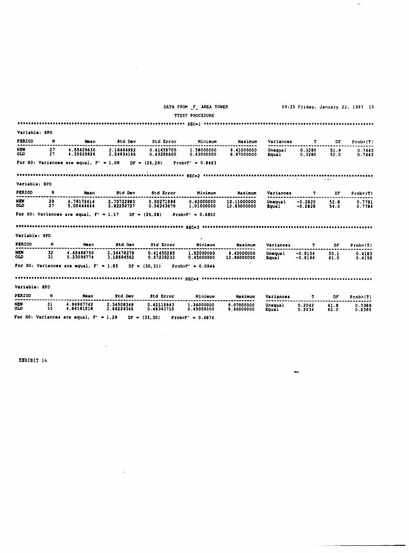
DATA FROH _F_ _ TOWER 09_25 Friday, January 22, 1993 15
TTEST PROCEDUR£
ttt_lltlttlt¢_Q_tlt_l_lttttttt_ttQtt_ttl_*_tttQtt_Atttttttlt SECI1 lilltt_ilttllltltQ_lliti_tQiill/llllilllt/lttlltltlttttttEttltt
Variablez SPD
PI_OD N Mean Std Dev Std Error Minimum Maximum Variances T DF Prob>lTI
NBIN 2? 4.$5629630 2.16464982 0,41650?05 1.58000000 9,41000000 Unequal 0,3280 51,9 0.?443OLD 2? 4.35825926 2.24934166 0,43288600 0,63000000 8.9?000000 F-_lual 0.3280 52,0 0,?443
For H0s Variances are equal, r' - 1,08 DF - (26,26) Prob>r' - 0.8463
************************************************************** 8ECm2 ***************************************************************
Variables 8PD
PERIOD R Mean Std Dev Sod Error Minimum Maximum Variancel T DF Prob>lTt......................... ..... .........
Nil/ 29 4.79172414 2.70?22983 0,50271996 0.42000000 12,11000000 Unequal -0,2820 52,8 0,?791OLD 2? 5.00444444 2.92250727 0,562436?9 1,01000000 12.83000000 ¢¢1ui1 -0,2826 54.0 0,??84
For H0t Variancea are equal, r' - 1.17 DF - (26,28) Prob>r' - 0.6902
******tttttt*********titt_*****t*t***t**l***_*ll*tttl,flttt,l,t 8ECB3 mlttlt***t****tt**t***t*****tl****lt**titttt,t***t,tlt**t******
Variables SPD
PERIOD N Mean 8¢d Day 8td Error Minimum Maximum Variance_ T Dr Prob>lTI
NEW 32 4.65468?50 2,344?82?9 0.41450295 1.52000000 8,65000000 Unequal -0,8154 55,1 0.4183OLD 31 5,23096??4 3,18694562 0,5?239233 0,45000000 12,96000000 Equal -0,8194 61.0 0,4158
For H0z Variancea are equal, r' - 1.85 DF - (30,31) Prob>r' - 0.0944
tttl*m_ittt**tttt*tt,l,t,l,tttt,t_tlt_,it_,tltt,ttt_o,tt_,_t _ECm 4 l*t*i_t_t_t_tt*_*t**t*iliti_tltit_It*lttii_i_Itl*_l_****li¢_
Variable_ 8PD
PERIOD N Mean Std Dev Std Error Minimum Maximum Variances T Dr Prob>lTI
N&II 31 4,9696??42 2,34508349 0,42118943 1,36000000 9,07000000 Unequal 0.2042 61,8 0,_389OLD 33 4.84181818 2.66224348 0,46343710 0,45000000 9,40000000 Equal 0,2034 62.0 0,8395
For H0_ Variancea are equal, F' - 1.29 Dr - (32,30) Prob>r' - 0.4874
EXHIBIT 1_
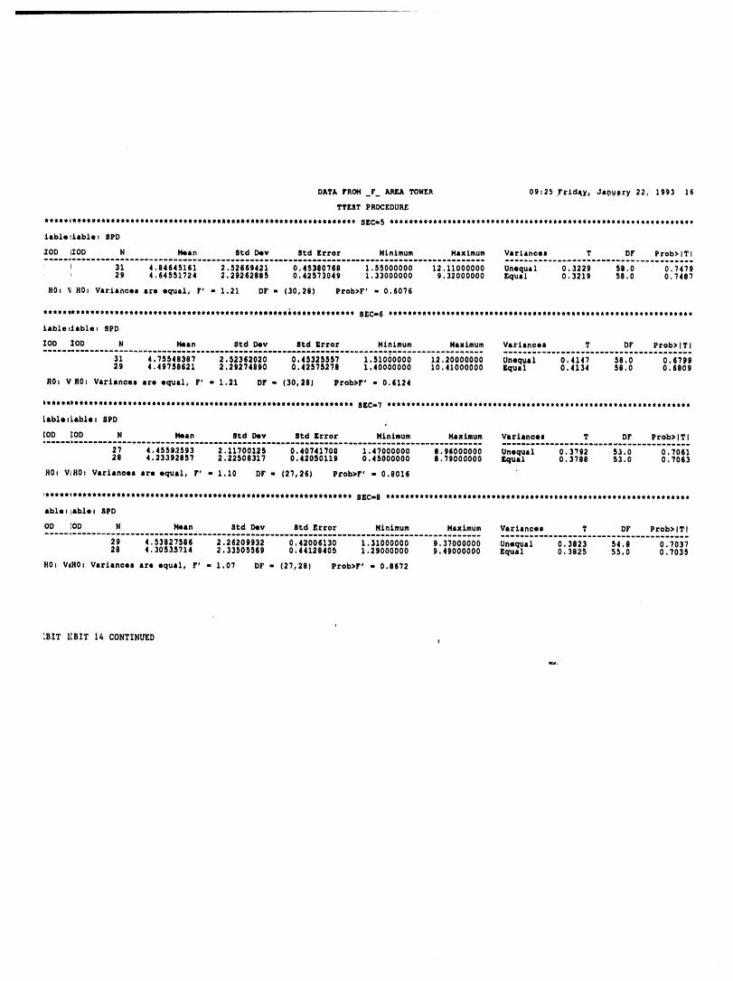
DATA FROM r AREA TOWER 09:25 .F_Id4yA OaOu_ry 22, 1993 16
TTEST PROCEDURE
)*et_e_ee_e_e_oee*e_et,teeee**eeee,ettt_e_etet,eteeee_**te,_teet, 9ECm5 ***************************************************************
'iable_iablel SPD
_OD _OD N Mean 8td Dev Std Error Minimum Maximum Variances T Dr Prob>tTI
I I 31 4.84645161 2,52669421 0.45380768 1,55000000 12.11000000 Unequal 0.3229 58,0 0.7479_ 29 4,64551724 2,29262985 0.42573049 1.33000000 9,32000000 Equal 0.3219 58.0 0.7487
H0: _ H0: Variances are equal, r' - 1.21 DF - (30,29) Prob>F' - 0.6076
*iltlltlltllttttRtttttltlt_tQttQQllltttlltlt_itt@_l_iiitllliit 8ECm _ tltt#Itltttil_ItttiliitltOtttiltt_RttttltlOt_iltmtli_/l_I/Rlilt
lableslable! SFD
ZOD IOD N Mean 8td Dev 8td Error Minimum Maximum Variances T DT Prob>lTI
31 4.75548307 2.52362020 0.45325557 1.51000000 12.20000000 Unequal 0,4147 50.0 0,679929 4,49750621 2,29274890 0.42575278 1,40000000 10,41000000 Equal 0.4134 58,0 0,6809
R0: V R0: Variances are equal, r' - 1,21 Dr - (30,28) Prob>F' - 0.6124
)ilili)iltlttt_lililiti_it_tli_tlilliillltii_lliiilili_i_%i_%ili_ _ECI 7 iiti_tliltltli_lilili_iiiliiliillllillllillllilt_llllillttilii
Lable:Leble: 8PD
[OD [OD N Mean Std Dev Etd Error Minimum Maximum Variances T DT Frob>lTI
27 4.45592593 2,11700125 0.40741708 1.47000000 8.96000000 Unequal 0.3792 53.0 0,706128 4,233928S7 2,22508317 0.42050119 0.45000000 $.79000000 Equal 0.3788 53,0 0,90_3
H0: VIH0: Variances are equal, r' - 1.10 DT - (27,26) Prob>F' - 0,8016
,sble|,sble| SFD
[OD [OD N Mean Std Dev Std Error Minimum Maximum Variances T DT Prob>lTIi .......................................
29 4.53827586 2.26209932 0,42006130 1.31000000 9.37000000 Unequal 0.3823 54.8 0.703728 4.30535714 2,33505569 0.44128405 1,29000000 9.49000000 Equal 0.3825 55,0 0.7035
H0: V_H0: Variances are equal, F' - 1.07 DF - (27,28) Prob>r' - 0.8672
IBIT IIBIT 14 CONTINUED
_..
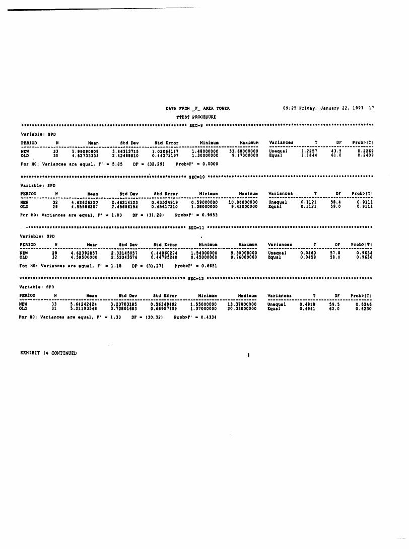
DATA FROH r ARF_ TONER 09:25 Friday, January 22, 1993 17
?_EST PROCEDUR_
ttottttJteJteQtttt/QtQJtttetttttttttQttttJettQetttttttQeeteJtt 8Eta9 tQQteettttttttttetteeettttttttttetetttttt_ettt_e,JtQtttttttt_i_
Variable: BPD
PERIOD N Mean 8td Dev Sad Error Minimum Maximum Variances T DF Prob>lTI
_;.,;......... ;;..... ;3;;;;;;;..... ;_;;;_;;;;..... [3;;;;_;..... _;;;;;;;;....;;_;_;;_;;_ ;_:_r ..... _;;_;..... ;;_;...... ;_;;_;OLD 30 4.62?33333 2,42400810 0,44272197 1.30000000 9,17000000 Equal 1,1844 61,0 0,2409
For H0: Variances are equalt r, - s,85 Dr - (32,29) grob>r' - 0,0000
IttltttltltttltllltlttQltliilttlilltltlltttNtl_t_tltI@_llltt@t _[Cml0 ItltlllllOtllttlttlitltlllllQtllttltittlt,ttttllttlttlttittllt
Varlsblet SPD
PERIOD N Mean Bad Dev Bad Error Minimum Maximum Varianoea T Dr Prob>tTi
OLD 29 4.5558620? 2.45_S_194 0,4S_17210 1.30000000 9.41000000 Equal 0.1121 59.0 0.9111
For H0: Variances are equal, r' - 1.00 Dr - (31,28) Prob>r' - 0,9953
_t_tttttJltt_ttt_t_j_ttttltttJtltttttttltlt_tllttttlitttitt _ECm11 tlt/ttltttettt_tttttttttt_lttlillttJJJlttttttttttttttttJttttll
Variable: 8PD
PERIOD N Mean 8_d Dev Bad Error Minimum Maximum Variances T DF Prob>lTj
NEW 28 4,623920S? 2,3314505? 0,440102?4 1,$4000000 9,30000000 Unoqua_ 0.0460 $?,| 0.9134OLD 32 4.59500000 2,533435?6 0.44?0S240 0.45000000 9,76000000 _rual 0.04S8 $8.0 0.9_36
For _0_ Variances are ecF_al, F' - 1.18 DF - (31,27) _rob>r' - 0,6451
ttllttt_ttti_tttlttttt_ttttt_tttt_ttttitttttttttetttttttttttt _ECu12 ttttttttttttttttttttJ_ttJtttttltttttitttttttt_tttJ_tOttJl_ttit
Vsrlable: EPD
PERIOD N Mean Bad D_v 8td Error Minimum Maximum Variances T Dr Prob>lTI
NEW 33 5._4242424 3,23?03105 0,8_349492 1,55000000 13,37000000 Unequal 0.4919 $9,S 0,_24_OLD 31 5,21193548 3.72401683 0.$6957159 1.37000000 20,33000000 r.qual 0,4941 62,0 0.6230
For H0, Variances are equal, r' = 1.33 Dr = (30_32) Prob>r' - 0,4334
EXHIBIT 14 CONTINUED I
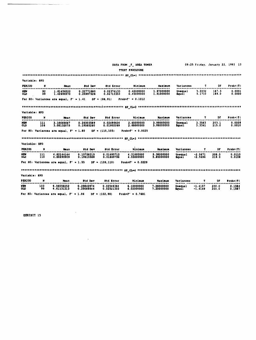
DATA rROH .r _ I_DH£R 0g,2_ rr;day, January 22, 1993 13
?T£S_ P_OC£DUP.t
tttttttltlttttotttttlttltttttttttt_lltilttttettttttlttitlledt _p _ _eatlejeeeooe_e_o_tooome_eoDottoooteeotteeteeeeoooeetoeoeoooeo
VtrLible; SPD
PERIOD N H, an BEd Dev |td Error HlnLmum Nix/mum VlrLln_el T DF Prob>lTI
OLD 99 1.42896|70 0,28997536 0.03713353 0.45000000 1.91000000 rx;u81 s.1710 ;89.0 0,0000
rot HOt V,=Lances are equal, r' - 1,41 Dr - 698,91) Prob)r' - 0.1012
OtOtttOtttttttJOOOttOtttttttttttOtOIttOttitOttttettttiOOttJtJ J_ _m 2 ttit_titQtetettJtttttttttttttttttttetttJtoJteowelleeiiJieJJe_o
VarLablo: BPD
PLqJOD N N.an BEd DQv BEd Error NLnLnun ;4axLeum YarLJn©es T or erob)ltl
NEW 111 3,18661d67 0._6303589 0,02496626 2.80000000 3,99000000 Onequ, l 3.3583 203.1 0.0009OLD 106 3.0013a0?5 0.19505a60 0.01902269 2.88000000 3.99000000 h_.Jal 3.3341 a15.0 0,0010
For H0_ VarLsnoel are equal, r' - 1.90 Dr - 6110,105) P_ob>r' - 0,002s
litii_te_eit_lilile_iJtti_ii_iieittittile_itiiite_etitltie_t _p C_3 _liiellilolott_tiitileitl_etielileteilteo_eeeeiieliitiiii|ttt
VtrLablet 8PD
Pit.DO N _an |_d Dev Std Error NLnLnun HaxLnus VsrLinoes T Dr Prob)(T/mmaeo_e.mmuaamm_mmmmm_ _ O_e_mmaammeeo_uu_mm_eemm_meabem_emauammom_ammmmom_m*U_m_ _mem_ee_om_mmem_muo.o*mmu.mommmuem_mo
hEW 111 4,8_144144 0.15758315 0,01495713 4,31000000 5.39000000 Onequl_ -_,5871 _00.5 0.0110OLD 110 4,89=90909 0.19810509 0.0116|796 4.53000000 5.15000000 r_iual -_,5696 21_.0 0.0108
rot H0_ virLJn_** are equal, r, - 1.55 Dr - (109,110) prob>r' - 0,0229
tttetttttteJeteettJJteettttteJettt,ttjtttttttttotmjteeOttoeet 8P_4 tetttttttteoeloot,eottetottoteteoeieteeoeteeottttttoetttttoote
VJ_&blet 8PD
PILq4OD N 14ein led DQv a_d Error N/nLnum HaxLmum VjrL_n=ee T or Prob>lTI
103 6,56058252 0.26042974 0,02546384 6.10000000 7.24000000 Oneq_,l -1.4157 200.0 0,15t4OLD 9g 8.81131313 0.25006644 0.02521303 6.02000000 7.20000000 _x;_l -1.4149 200,0 0.158?
rot n0_ Ys_Lan¢om are equsl, r' - 1.08 Dr - 6102,98) e_ob>r' - 0.7681
EXHIBIT 15
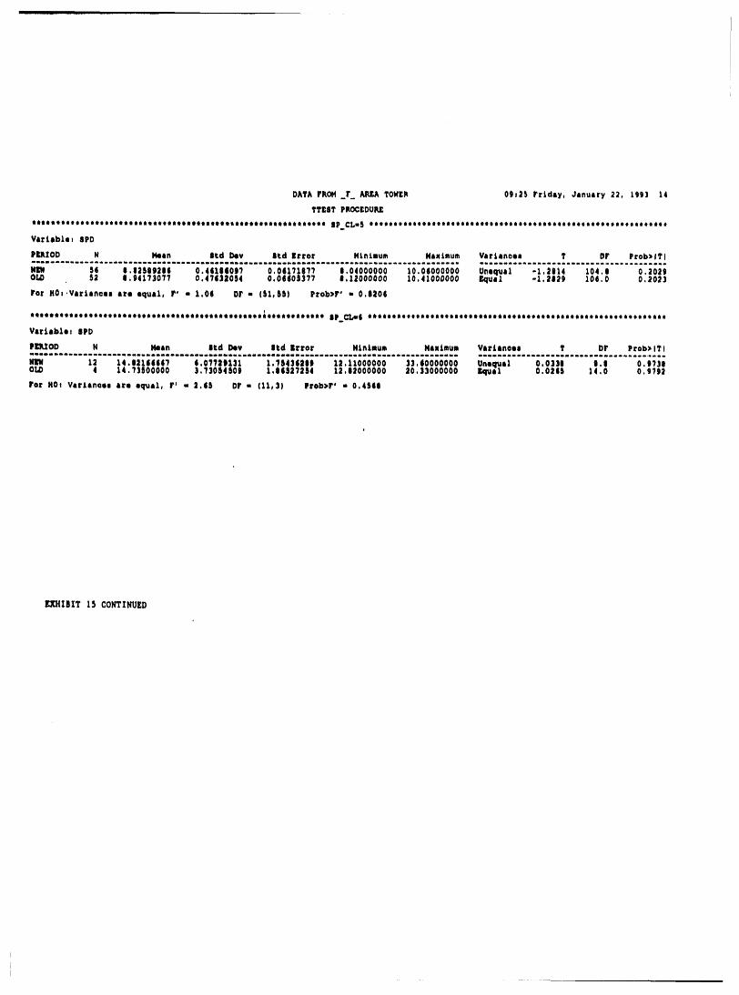
DATA rRoH r_ MUr,A TOWER OQI_S friday, Jmnuary 22, Lgg3 14
TTEaT PROC[DUI_
o_laeoeeeoo_etooooeQ_ttotttoo_o_oeQoteiit_iQoeQetotQQo_Qeo,oo _C_m_ oteooeoeetteooeeoo_tolo,iieoelooQo,ooooQ_ee_e_e_,_
Va_L_bl,_ |PD
PUIOD N Heln ltd Dev ltd Itror N[nLium Nix{mum VltLmnoem ? or frob)lfl
m 5t i.taSii2|l 0.411110Q9 0.01111819 t.04000000 10.0t000000 Uneau,l -1.2114 104.i 0._0_tOLD 5a 8.941130?? 0.47i|a054 0.0_i0S$?7 8,12000000 10.41000000 I_ru_l -1.2029 10_.0 o.3033
rot HO_.Va_Lsflces are equal, r' • 1,0t Dr - (Sl, SS) erob>r' - 0.e_o_
************************************************************* I_.CLel **************************************************************
VioLable! _PD
_I_ZOD N Heart I_d Dev |_d |_tor HLnLmum NaxLm_a VirLinaem Y Dr Prob)lTI_e__e_me_m_m_mem_mem_s__m_mmmmamemmeee_eee_m_m_ Bmmm_ee_me_mmmwm_mm_me_mm_m_e_me_e.
Ifl_ 12 14.1_16_ti_ 1.077_131 1.TSi]i_it 12.11000000 23.10000000 Unecm, l 0.0331 m.t o._731OLD 4 14.73S00000 3,7]054S0i _,I_S_?_S4 12,I_000000 _0,33000000 _1 O.02iS 14,0 O,_?S_
ro_ HOt Vt_L_naem l_l equil, r* - _.i5 Dr - (1_,3) _rob)r* - 0.4Sil
EXHIBIT 15 CONTINUED
I
i
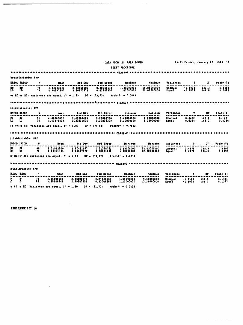
DA_A rMo,4, _ _M 13,23 rr,day, J,nuJry 22, ;003 11
YTE|T Plq,O_:_OUIqJ,
ililtllliltlliliiiiliitliiiililliielililiiliiiliilitiitililliliili ¢_JJm A lililiiliiffiliitililiiilililiiilliiillilllilllliliiiitiilOilil
_r_Abl'lr_Ablet |PD
nIOD RIOD H Mean 8td i_y 8td Error HtnLmus Maximum VartaneeJ Y Dr Prob)lTI
bD 74 4.t42|72|? 3.I0i70_?1 0.4ii11tS3 1.41000000 12.010b0000 Kqual -0.1016 146.0 0.S404
or R0_or R0_ Viriinae, ire eqUilo r' . 1.i5 or - (13,131 prob>r' - o.oo4s
ItJitiliJitiJiliiilQiitiilittJiililiililitiiliililJiitiiJlJiJiiJOJ C_lta iOiJtilitJi|eOiJii*iitiJitiJiiitlJtiiitlitiii|tiliJeioileoilit
irtablirtablet IPD
i_XOD JI_tZOD N I_lln Itd Dev itd |trot NinLmum HauLmue VsrLinael ? Dr Prob)lTI_m_mmm_m_mmmum_m_u_Imum_m_m_ammmmm6_Im_mmmmm_m_am_m_mI_mmm_mmmmmmum_mummmmu_m_m8_m_mmm mmm_O_mmm_mmmmmmII._Dmmammm._m.wmw_I.
,,,o,oooo,,.,,,,, ,,oooooo,,ooooooo o,,o, ,,,, o,,,70 4.4581142D |.||0111Ot v._Ti|i|OD 1.|0000000 0.04000000 0.4314 14].O O.S_31
)r HOt)r HOt VarAanae, ire equal, r ° , 1.01 Dr o (74.||) Preb)r' o O.TES_
)tllilitlliillllililitlililittlilliliiliiitiilitlliiittitiililiili ¢_JS_ lilililliliililtiititilitiililliliiliiiiiilliiiliitliOilliiiil
hriabltriablet 8FD
_._OD _q_OD N i_ln Jtd Dev 8_d |rror HLntmue Haximum Varlan0e8 ? Dr Pr0b)lTI_e_m_me_m_mm_m__j_m__a__j_u_e_m_m_e__m_s_j uaJeaoeeoOsJt_Ooemae_6a_u_euJmaoeeeeme
N Io S.llJi_So0 J.|O411|i7 O.]I3Si?I: 1.4S000000 t4.03000000 Unequal 0.4_71 15S.! O.tiJ310 4.133717JS _.iSSi?]?| 0.30071i4D |.|iO00000 1].20000000 Equil 0.4|?¢ 1S4.0 0.44|S
_r HO_r HO_ Var_Jneem are eqU,lo r' - 1,1_ Dr - (1_,??) _rob)r° - 0.131!
)toweeftowoeeoewoesooe0iioeeeoooeJteoeieogeeomeototeotmeootoeeejit CLAj|mD **eiioooiteoeieotoeootiimeeeoeteoiteietoeetiieeoeotoitieiiitt,
ltLabiCtLabten IPD
_ZOD _ZOD N Mean ltd Dev ltd lrror H_n_mum Ha_Lmum VarLan©es ? Dr Prob)l?l
_ 02 5,30141341 _.SD|4TiS1 0.33041408 1.22000000 13.24000000 I_l_JIl -2.4|22 1S4.0 0,131T
Jr N01Jr N01VJrlanaeo ire equal, r' - 1.to Dr , (D1,13) Prob)r* - O.043S
U_TNIU_TNIT 16
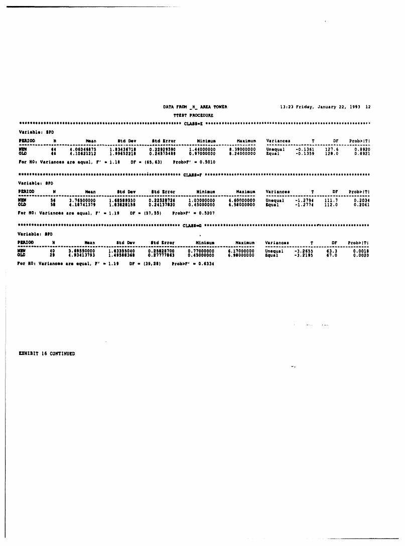
DATA rROH H _ I'OHER 13:23 friday, Januaz'y 22, 1993 12
TTEIT PROCEDURE
t0teet00eootJ0eeJee0eJ0toe00to00tte0te0teet0Joeee0N0e0eteo00t C_J_mE ete0ee0tt00J0toeeeoeto0e0t0tteeeeoeetee00eeeoo_eeettett0Qteo,,
VJriablet |FD
PlUI.TOD N iCean 8td Dev itd Error NLninum Haxtmum Variances T Dr Prob>lTI
64 4.0104iiTS 1.03436710 0.229295|0 1.44000000 8.19000000 Unequll -0.1361 127.6 0.0920OLD 46 4.i04a1212 1.J015|21| 0._4STS48g 0.iT000000 0.24000000 Equal -0.13_9 128.0 0.8921
for HOt Variinaes ire oq_Jl, r' - 1.10 Dr - (05,63) Prob>r' - 0.5010
ltilllttlllittllltttlilllllllltiltltillllllllltl6lllllltlllll ¢Lk�smr llltllttittltllltlllllllltllltllllltllltllltiltiltltllllltlllt
VlrJlblll IPD
PrJUOD N ICeln ltd D¢i¥ ltd irro_ NLnLuum NaxLaum VirLanoe| T Dr Prob>lTI_e_O_om_me_u_m_Bum_a_mm_Iu_u*D_ea_a_m_m_d_mu_a_nm_u_ eeee_n_eeeeou.eeoe.e_emuaeeo_umeeeeu.e
HI:H Si 3,71S00000 I,tISIiSS0 0.1|Sal?2t 1.03000000 6.10000000 Unequal -1.2T94 111.T 0.2034OLD 50 4.101413?0 1003|10150 0.34137030 0.45000000 4.50000000 I_qu,l -1.2TT4 113.0 0.2041
rot Hot VlrLanoel tre equaL, r' - 1.10 Dr - (5?,5S) rrob)r* - 0.5207
liiJllllillitlttltiiltJllltlltitllllltlllltllltlllltttltlltll {_1_ llllllliltlllllilililltttllllitlltltJliitll_itttllttlltlltttlll
VlrLlblo| IPD
PJU_OD H Neln ltd Dev 8td Error Hlninui Haximum Vlrlin{el T Dr Pr0b>lTiM___u_I_e_mu_m_o_me_e_m_mm_m_m_mmm_e_mm_m_ _U_OuoJume_6oeu_eoaee_o_uo6emnomu_eu
40 3.l|SSO000 1.633SS040 0.i0820700 O.T7000000 0.17000000 Unequal -3.2655 63.3 0.0018OLD 2i 4.034137i3 1.4i0083t0 0.|7777103 0.40000000 t.t8000000 l:qu,l -3.2105 6?.0 0.0020
rot i0| VariJnae, Jr, equal, r' - 1.1t Dr - (39,21) Prob)r' - 0.6334
F._IBIT 16 C01_TINUEn

DA?k rROH H JUU_, TONI£R 13:23 Friday, January 22, 1993 15
?TEST PROCEDUI_
Itteetitteetoottlttt_tltotQ_ttotttot_tt_tttlmotiItoottttotttlttto_oJ 8_CI1 itoitttettltttteetmtttotttJtooellttooettttttt_QItttt#_tttteletl
rariab_sriablet |PD
PnXODPI_XOD N Nean 8td Dev 8td Zrwo: HLntnun HaxLmum VacUa,tea T Dr Prob>lTI
_ 25 4.18280000 2.00338900 0.4008??9| 1.53000000 e. S4000000 Unequal -0.3107 4S.g 0.75?3)I4) 2? 4.36621)630 2.25489408 0.4339545? 1.22000000 9,34000000 r,qual -0.3092 So,0 0._594
)or HOtor HOs VarLin=ee are equal, r' - 1.27 Dr - (26,24) Prob>r' m 0.5633
Iflllttltllttltt_tttiltiliOttflttltttDtltlttttttRttllttt_ttttttlttlttt 8[Ce2 tttltttttltlottttlttletttttttltttttttllttotltltenttttttotlttto|
llrLJb_lrLJb_et |FD
'IM_XOD2U_OD N 14eJn Bid Dev 8td 1trot NLnLmus HtxLmum VirLlnoee T Dr Prob>lTl
I_ _ 30 4,72833333 2,2816102_ 0.41656314 1.50000000 8.?4000000 Unequal 0.4103 54.2 0.4714LD 2? 4,4729629_ 2,31931657 0.44635960 1.40000000 10.10000000 IMIull 0.4106 SS.0 0.6711
or HOtor HOt VarLinoee are equaL, r' - 1.03 Dr - (26,29) erob)r' - 0.9267
tiJttiliJttiittttlittttilttttlttttJtttttltttJttititijliltlttttJtttj _Ca 3 tftltltlitttttttttttOtJtttttlttttttOJtttttttJttettitiJtttttltit
|rLabl|rLable: SPDo
r,RXOD r,RXOD N Menn _ ,_ D41v 8_d Erro_ NLnLnum HJxLmum Vlrllnce8 T Dr Prob>l?lm
_ 30 4.592i6647 2.3?36?885 0.4333?248 1.43000000 9.30000000 Onequ, l . _:5_ .... ;_,9 0,59?24,.... 0.,.,. 0.000000,.000000..., .0 0,,._r H0t_r HOt VsrLJnoen are equaL, r' - 1.07 DT - (29099) Prob>r' - 0,|6_5
_tttit_tttitlitttlttittttltttttitttttit_ttlittttt_Ittlltllttilelli _4 _e_tt_tt_tootoeetoeooooete_totetteoee_toe_etoOteeoooJeeoettt
irkabltrkable_ SPD
_OD J31,TOD N Nean 8td Dev |_d Error NLnAmun XaxLnua VsrLances ? Dr P_ob)l?l
2? 4.30952943 2.09?24450 0,403614|9 1.31000000 0.8100000026 4.40230?49 2,01192308 0.3945?050 1.22000000 8.11000000 £qual -0.1_41 51.0 0.9?03
)r HOt)r HOt Va:Lances are equal, r' - 1.09 Dr - (2_,25) Prob>r' - 0.037_
XHIBI'I_IBIT 17
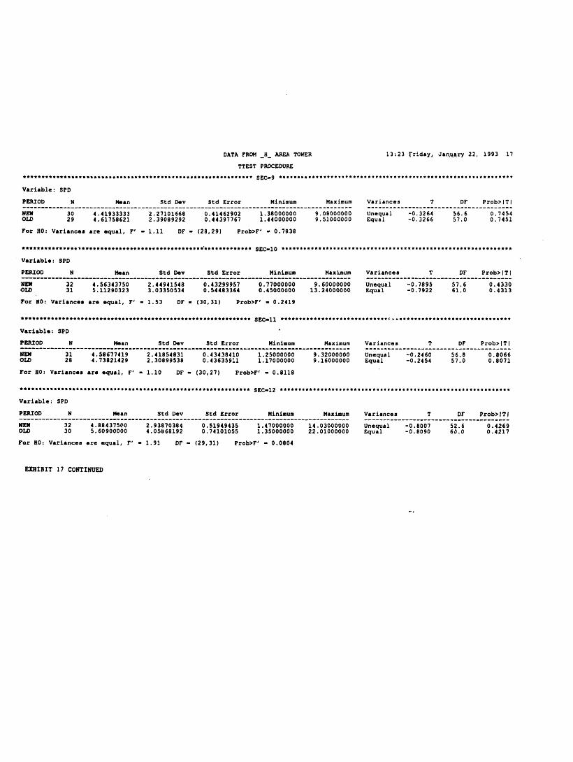
DATA FROH H AREA TOWER 13:23 Friday, Ja_qAry 22, 1993 17_ _
TTEST PROCEDURE
tet_tttttttttttmttttttt*wtt_t_t_ttt_tt_ttttttttttottttemeI,tt SECm9 eQt_t_ttt_tet_tttt*tt_**ttt*t*t*_wt_.t,tttt**tt,ttttt***t,t*tt*
Variable: SPD
PERIOD N Mean Std Dev Std Error Minimum Maximum VarLances T DF Prob>ITl........................... . ....... ...-
NEW 30 4.41933333 2.27101668 0.41462902 1.35000000 9.08000000 Unequal -0.3264 56.6 0.7454OLD 29 4.61758621 2.39089292 0.44397767 1.44000000 9.51000000 Equal -0.3266 57.0 0.7451
For H0: Variances are equal, F' - 1.11 DF - (28,29) Prob>F' - 0.7838
Variable: SPD
PEI_/OD H Mean S_d Dev Std Error Minimum Maximum Variances T DF Prob>ITl
NEW 32 4.56343750 2.44941548 0.43299957 0.77000000 9.60000000 Unequal -0.7895 57.6 0.4330
OLD 31 5.11290323 3.03350534 0.54483364 0.45000000 13.24000000 Equal -0.7922 61.0 0.4313
For B0: Varlance_ are equaZ, F' - 1.53 DF - (30,31) Prob>F' - 0.2419
Variable: SPD
PERIOD H Mean S_d Dev S_d Error Minimum Maximum Variances T DF Prob>lTl
NEW 31 4.58677419 2.41854831 0.43438410 1.25000000 9.32000000 Unequal -0.2460 56.8 0.8066OLD 28 4.73821429 2.30899538 0.43635911 1.17000000 9.16000000 Equal -0.2454 57.0 0.8071
For B0: Variances are equal, F' - i. I0 DF - (30,27) Prob>F' - 0.8118
Variable: SPD
PERIOD N Mean S_d Dev S_d Error Minimum Maximum Variances T DF Prob>ITl
NEW 32 4.88437500 2.93870384 0.51949435 1.47000000 14.03000000 Unequal -0.8007 52.6 0.4269
OLD 30 5.60900000 4.0586G192 0.74101055 1.35000000 22.01000000 Equal -0.8090 60.0 0.4217
For H0: Variances are equal, F' - 1.91 DF - (29,31) Prob>F' - 0.0804
EXHIBIT 17 CONTINUED
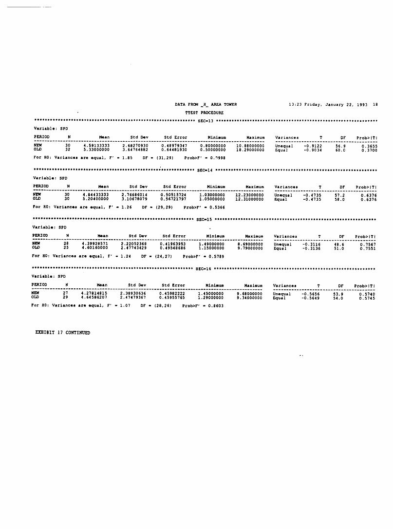
DATA FROM _H_ AREA TOWER 13:23 Friday, January 22, 1993 18
. TTEST PROCEDURE
ttftetttttttltttffettttttt_tttttttttttttttttt.ttttttttttttttttt SEC-13 tttttttttllttlttttttttttttttttttttttttittttttttttttttttttttltt
Variable: SPD
PERIOD N Mean Std Dev Std Error Minimum Maximum Variances T DF Prob>ITi............ . ............ . ........................................................................................... . ...........
NEW 30 4.59133333 2.68270930 0.48979347 0.80000000 10.88000000 Unequal -0.9122 56.9 0.3655OLD 32 5.33000000 3.64764882 0.64481930 0.50000000 18.29000000 Equal -0.9034 60.C 0.3700
For H0: Variances are equal, F' - 1.85 DP - (31,29) Prob>P' - 0._998
ttttttttttttttttttttttttttttttttttwtttttttttttwtttttttlttttttt SECml4 ttttttttQtttttttttlWttttttttttttttttttWttWttttttwtttttttltettt
Variable: SPD
PERIOD H Mean Std Dev Std Error Minimum Maximum Variances T DP Prob>ITl.............. . ........................
NEW 30 4.84433333 2.?6686014 0.50515724 1.03000000 12.23000000 Unequal -0.4735 57.2 0.6376OLD 30 5.20400000 3.10678079 0.56721797 1.05000000 12.31000000 Equal -0.4735 58.0 0.6376
For R0: Variances are equal, F' - 1.26 DP - (29,29) Prob>P' - 0.5366
tttttttttttttttttltt*ttttttt*ttttttttttttttttttttttttltttttttt S_Cm15 tttttttttttttetttttttttttttttttttttttttttttttttttltttttttttttt
Varlable: SPD
PERIOD H Mean Std Dev Std Error Minimum Maximum Variances T DP Prob>IT#... ................................................ ... ....... .... .... ... ........................................................
NEW 28 4.39928571 2.22052368 0.41963953 1.49000000 8.69000000 Unequal -0.3116 48.6 0.7567OLD 25 4.60160000 2.47743429 0.49548686 1.15000000 9.79000000 Equal -0.3136 51.0 0.7551
For H0: Variances are equal, F' - 1.24 DF - (24,27) Prob>F' - 0.5789
tttltttlttttttttttttttttttltttttttttttttttttttttttttttttttlltt 5EC-16 llllllllllllllilllllllllllltlltlmltllllllllllllllllllllillllll
Varlable: SPD
PERIOD N Mean Std Dev Std Error Minimum Maximum Variances T DF Prob>ITl.......................................
NEW 27 4.27814815 2.38930636 0.45982222 1.45000000 9.68000000 Unequal -0.5656 53.9 0.5740OLD 29 4.64586207 2.47479367 0.45955765 1.29000000 9.34000000 Equal -0.5649 54.0 0.5745
For H0: Variances are equal, F' - 1.07 DF - (28,26) Prob>F' - 0.8603
EXHIBIT 17 COI_rlI(UED
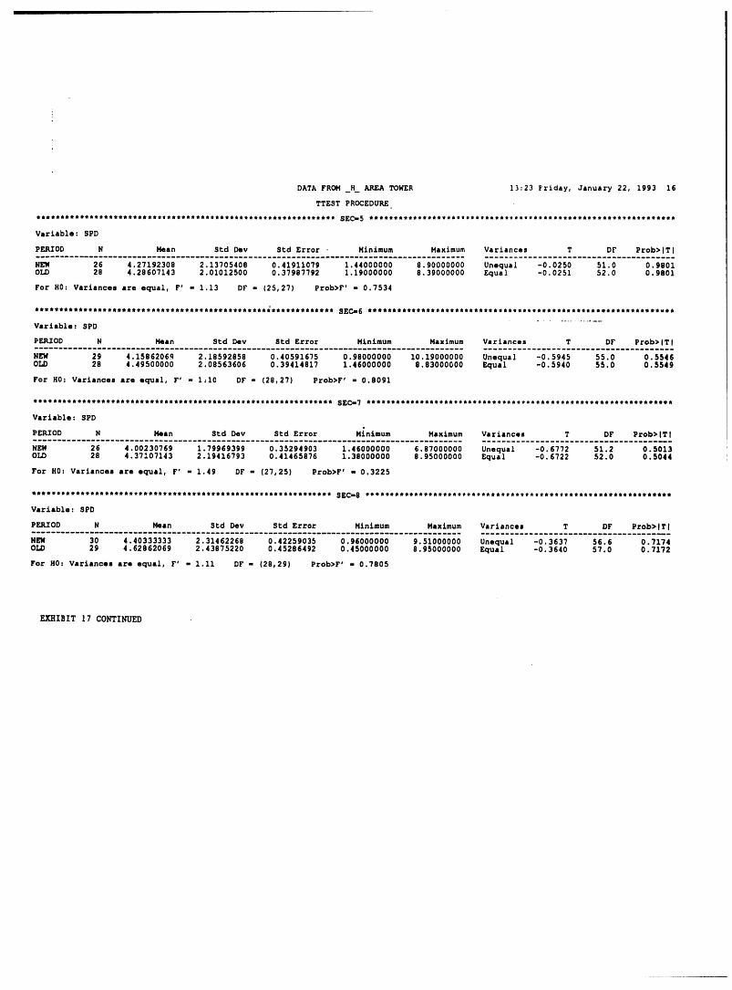
DATA FROM _H AREA TOWER 13:23 F'riday, January 22, 1993 16
TTEST PROCEDURE
tttem_t*****_**tttt**t_,_,t_t*tttttt*********tt**tttltt,tt_e_ SECm5 **t*t_tttt_***t*_*_*w**_ttttttt_e_*wwt*t_tttmtm*_t,mt_tet,
Variable: SPD
PERIOD N Mean $td Dev $td Error • Minimum Maximum Variances T DF Prob>ITl............................... ._..__..
NEW 26 4.27192308 2.13705408 0.41911079 1.44000000 8.90000000 Unequal -0.0250 51.0 0.9801OLD 28 4.28607143 2.01012500 0.37987792 1.19000000 8.39000000 Equal -0.0251 52.0 0.9801
For H0: Variances are equal, F' - 1.13 DF - (25,27) Prob>F' - 0.7534
• ************************************************************* SEC-6 ***************************************************************
Varlable= SPD
PERIOD N Mean Std Dev Std Error Minimum Maximum Variances T DF Prob>ITl
NEW 29 4.15862069 2.18592858 0.40591675 0.98000000 10.19000000 Unequal -0.5945 55.0 0.5546OLD 28 4.49500000 2.08563606 0.39414817 1.46000000 8.83000000 Equal -0.5940 55.0 0.5549
For H0: Varlancea are equal, F' - i_I0 DF - (28,27) Prob>F' - 0.8091
Variable: SPD
PERIOD N Mean S_d Dev Std Error Minlmum Maximum Variances T DF Prob>ITl
NEW 26 4.00230769 1.79969399 0.35294903 1.46000000 6.87000000 Unequal -0.6772 51.2 0.5013OLD 28 4.37107143 2.19416793 0.41465876 1.38000000 8.95000000 Equal -0.6722 52.0 0.5044
For H0: Varlances are equal, F' - 1.49 DF - (27,25) Prob>F' - 0.3225
Variable: SPD
PERIOD N Mean Std Dev Std Error Minimum Maximum Variances T DF Prob>ITl
NEW 30 4.40333333 2.31462268 0.42259035 0.96000000 9.51000000 Unequal -0.3637 56.6 0.7174OLD 29 4.62862069 2.43875220 0.45286492 0.45000000 8.95000000 Equal -0.3640 57.0 0.7172
For H0: Varlances are equal, F' - I.II DF - (28,29) Prob>F' - 0.7805
EXHIBIT 17 CONTINUED
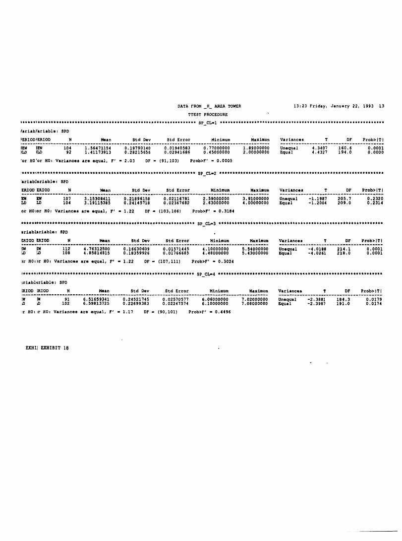
DATA FROH H_ AREA TOWER 13:23 Friday, January 22, 1993 13
TTEST PROCEDURE
_ariabYariable: $PD
_ERIOD_ERZOD N Mean Std Dev Std Error Minimum Haxlmum Variances T DF Prob>ITl..... ...... ..__.....___. ....... . ....... . .... . ........... . ............ . ...... .. .... .._... ...... ._...._.... ..... ...........__...._._...
IEW IEW 104 1.56471154 0.19790140 0.01940583 0.77000000 1.89000000 Unequal 4.3407 160.6 0.0001_LD )LD 92 1.41173913 0.28215656 0.02941686 0.45000000 2.00000000 Equal 4.4327 194.0 0.0000
_or H01bor H0: Variances are equal, F' - 2.03 DF - (91,103) Prob>F' - 0.0005
Jariab_'ariable: $PD
ERIOD ERIOD N Mean Std Dev Std Error Minimum Maximum Variances T DF Prob>ITl
EW EW 107 3.15308411 0.21896158 0.02116781 2.59000000 3.91000000 Unequal -1.1987 205.7 0.2320LD LD 104 3.19115385 0.24145718 0.02367682 2.63000000 4.00000000 Equal -1.2004 209.0 0.2314
or H0:or H0: Variances are equal, F' - 1.22 Dr - (103,106) Prob>F' - 0.3184
_riabl_riable: SPD
_RIOD _RIOD N Mean Std Dev Std Error Minimum Maximum Variances T DF Prob>ITl
_W _ 112 4.76312500 0.16630609 0.01571445 4.10000000 5.54000000 Unequal -4.0188 214.1 0.0001_D i08 4.85814815 0.18359926 0,01766685 4.48000000 5.43000000 Equal -4.0261 218.0 0.0001
>r H0:>r H0: Variances are equal, F' - 1.22 DF - (107,111) Prob>F' - 0.3024
_rlablQrlable: SPD
IRIOD IRIOD N Mean Std Dev Std Error Minimum Maximum Variances T DF Prob>jTj
l* IN 91 6.51659341 0.24521745 0.02570577 6.06000000 7.02000000 Unequal -2.3881 184.3 0.0179
_ 102 6.59813725 0.22699383 0.02247574 6.10000000 7.08000000 Equal -2.3987 191.0 0.0174
,r H0:Ir H0: Varlances are equal, F' - 1.17 DF - (90,101) Prob>F' - 0.4496
EXIilI EXIIIBIT 18
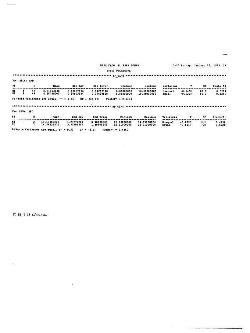
DATA FROM H AREA TOWER 13:23 Friday, January 22, 1993 14
TTEST PROCEDURE
Vs: SPDm: SPD
P| ! N Mean Std Dev 8td Error Minimum Maximum Variances T DF Prob>ITl._ .... .,-........-............_.__.__.. ............. .........-..-........................ ..... ....... . ........... .... ......... ..
N| 4 47 8.81063830 0.63087036 0.09202190 8.01000000 10.88000000 Unequal -0.6430 87.0 0.5219OX 4 44 8.88750000 0.50603854 0.07628818 8.08000000 10.34000000 Equal -0.6384 89.0 0.5249
F_Varia Variances are equal, F' - 1.55 DF - (46,43) Prob>F' - 0.1473
************************************************************* SP CL-6 **************************************************************
Va: SPD_s SPD
PI J N Mean Std Dev 8td Error Minimum Maximum Variances T DF Prob>ITl
N_ i 2 13.13000000 1.27279221 0.90000000 12.23000000 14.03000000 Unequal -0.8720 6.2 0.4158O_ 7 14.64428571 3.92909598 1.48505869 12.11000000 22.01000000 Equal -0.5147 7.0 0.6226
F_VarlalVarlanoes are equal, F' - 9.53 DF - (6,1) Prob>F' - 0.4860
IT 18 IT 18 C_NTINUED
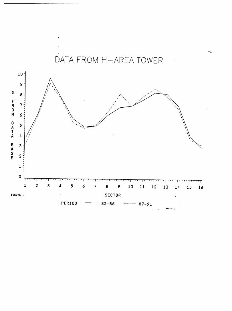
DATA FROM H-AREA TOWER ,
I0
9
FR 70
M 6 /DA 5TA 4
B 3ASE 2
i
0' ' ' ' 1' ' ' ' I ' ' '" I ' ' ' ' i .... I ' ' '' I ' ' ' ' I ' ' ' ' I ' ' "' J ' ' ' ' I ' "'" I ' ' ' ' I" '' ' I ' ' 'rl' ' ' ' I '
1 2 3 4 5 6 7 8 9 i0 ii 12 13 14 15 16
_'zcm_z SECTOR ,
PERIOD 82-86 ................87-91
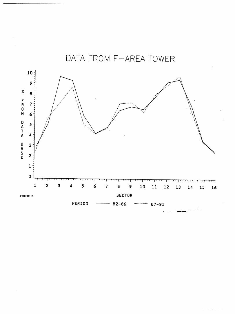
DATA FROM F-AREA TOWERo
10,*%
.,.. ,..,"" '""
_ 8
FR 70N 6
DA 5TA 4
B 3A ,SE 2
1
0' ' ' ' I' "" _ I .... I .... I ' ' ' ' I ' _ ' ' I ' ' '" I .... I ' ' ' ' I '' '" I ' '" ' I' ' "' I .... I ' "i'"'* I .... I
1 2 3 4 5 6 7 8 9 I0 ii 12 13 14 15 16
n_ 2 SECTOR
PERIOD 82-86 ................87-91
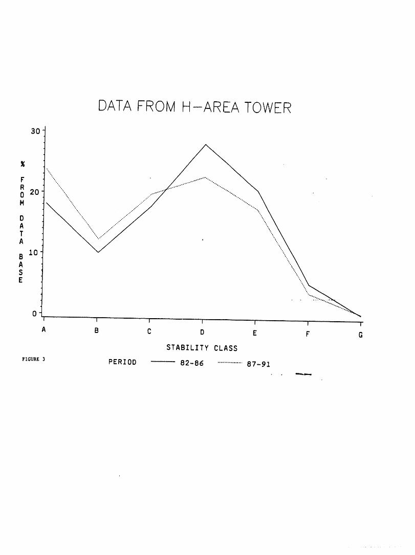
DATAFROM H-AREA TOWER
30"
0I i i I 'I i
A B C D E F O
STABILITY CLASS
FIGURE3 PERIOD 82-86 ................87-91-
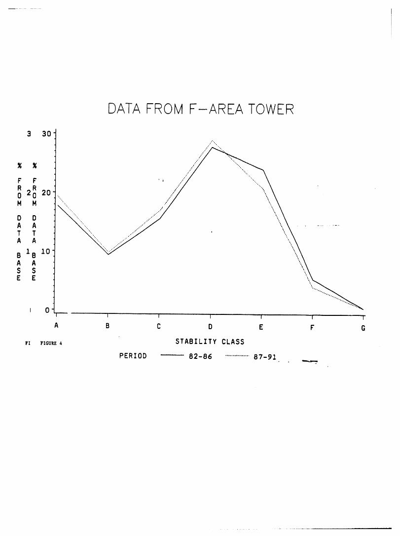
DATA FROM F-AREA TOWER
3 3O,,/',,
F" F"
0 2 20M M
D DA AT TA A
B 1B 10A AS SE E
i 0I I I I I •
A B C D E F" G
1'x FXGu_4 STABILITY CLASS
PERIOD 82-86 ................87-91
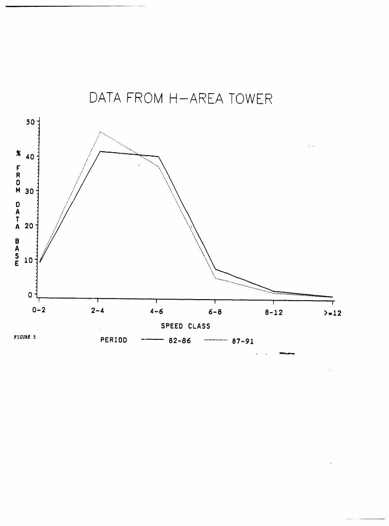
DATAFROM H-AREA TOWER
50"
40
F"R0M 30
DATA 20
BA$E 10
............... i i i I II i i
i I i " i t
0-2 2-4 4-6 6-8 8-12 >=12
SPEED CLASS
FIo_ s PERIOD 82-86 ................87-91
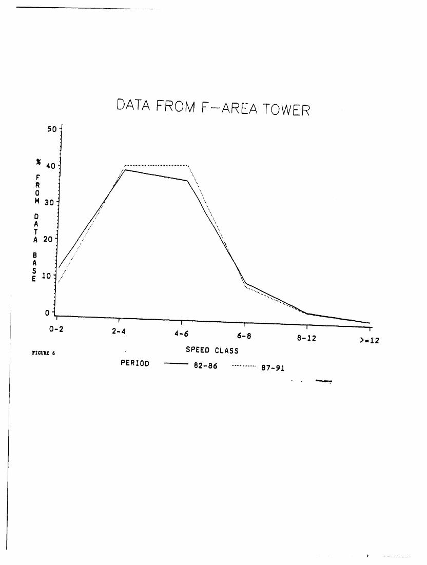
DATA FROM F-AREA TOWER50
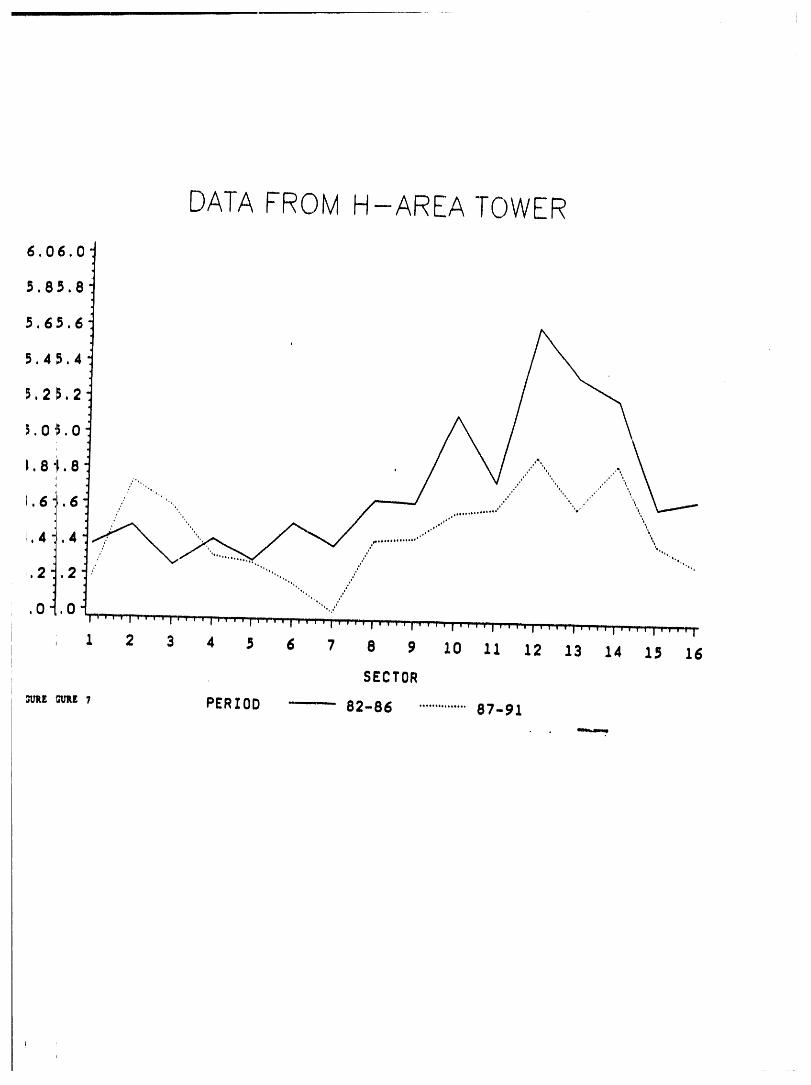
DATA FROM H-AREA TOWER
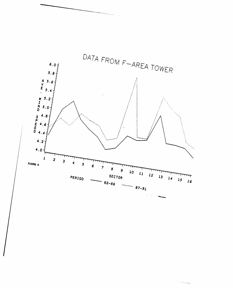
DATAFROM F-AREA TOWER
6.05,8
x
A 5,6 / '..
E _.4 , : '.. ,
!N 5,0 , / '_ / "..
"-.... i ; / ',S48 ....... _. _ :./.- _,.../ \ ,.. _ ,, // \ ',..p ", .,,_ '.. _ _ _. ....J./ \ .....E46E04.4
4.2
4.0 i:' ;' ' i ' ' ' "'i''-_,;i ' ' '' I ' ' ' 'i ;' '"i;' ' ' _' ' ' ' I ;; * ' w'"; ' i ' ' ' '"i _';' ' i .... ! ' ' ' ' I ' ' ' ' i
1 2 3 4 5 6 7 8 9 10 11 12 13 14 15 16
rzmnc¢8 SECTOR
PERIOD ........... 82-86 ..............87-91
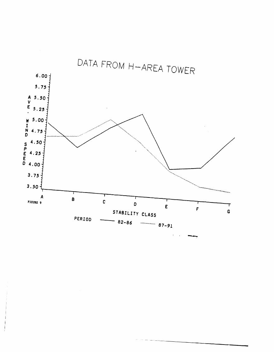
DATA FROM H-AREA TOWER
6.00
A 5.50V
E 5.25m
W 5.00
N 4.75D
S 4.50PE 4.25E
D 4.00 ..........................................3 75 ..........
3.50
A B C D E r GFIOUI_ 9
STABILITY CLASS
PERIOD ..... B2-86 ................87-91
i i,,
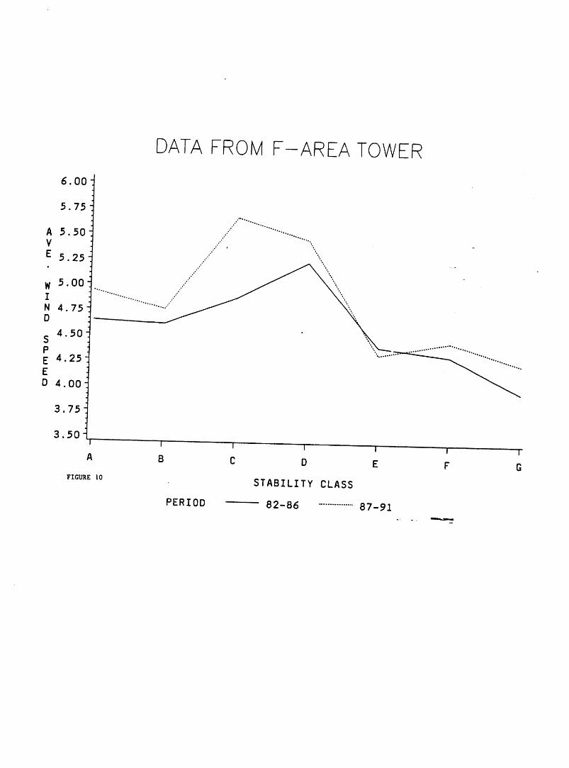
DATA FROM F-AREA TOWER
6.00
5.75o,._'.o,,o°
o "'...,.,
A 5 50 "" ..............• .." '°°°°%
V "ooO.°." i
E 5.25 ""
W 5.00IN 4.75D
S 4.50PE 4.25 ................................ED 4.00
3.75
3.50I I I I I I
A B C D E F G
F_C_ElO STABILITY CLASS
PERIOD 82-86 ...............87-91
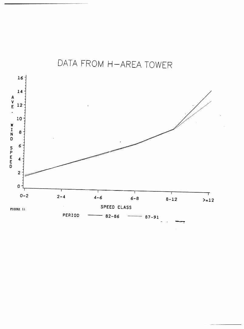
DATA FROM H-AREA TOWER
16
14AVE 12
i0
WIN 8D
S 6P
...°....,.,.°'"°°""°"
E 4ED
2
0I I I I I
0-2 2-4 4-6 6-8 8-12 >=12
SPEED CLASSFIGURE 11
PERIOD 82-86 ................87-91
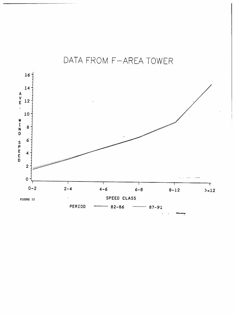
DATA FROM F-AREA TOWER
16
14
AVE 12
10
WIN 8D
S 6P
E 4ED
2
..............
I I I I I
0-2 2-4 4-6 6-8 8-12 >=12
FImmE12 SPEED CLASS
PERIOD 82-86 ...............87-91
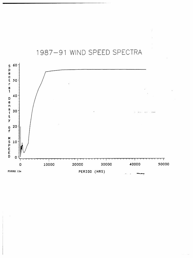
1987-91 WIND SPEED SPECTRA
S 6OPeot ._0ra1
4ODensi 30 ................tY
o 20f
MS I0PEE
D 0 ......... i ......... I ......... i ......... i ...... , , ,'"'r'0 .1.0000 20000 30000 40000 50000
FZGUm_13,,, PERIOD (HRS)
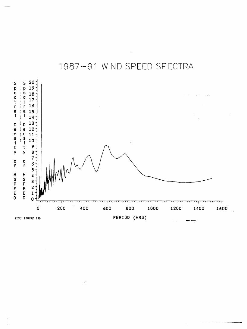
1987-91 WIND SPEED SPECTRA
SIS 20p ;p 19e,el8C , Ct ,t 17r ir 16
'a 15-a ,
11114"
01013e le 12-n In IiS
i I_ I0t t 9y y 8
70 0
f f 65
M M 4
S S 3 _P PE E 2E E 1O O 0
,"r'j,, ,, f, i,r',,,,,, , i,, w, ,,, ,,,i,,,,, ,T,, i, , ,, ,, ,,,i,, ,,, ,,,,, i,,,, ,,, ,,i,,,, , ,,_ , !
0 200 400 600 800 I000 1200 1400 1600
FIGI_FIGD'R_13b PERIOD (HRS)
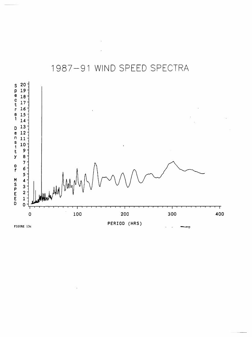
1987-91 WIND SPEED SPECTRA
S 20[p 19e 18-Ct 17
r 16"
a 15-l 141
D 13e 12-n ii isi i0t 9y 8
70f 6
5M 4
p[ 2E 1D 0
0 100 200 300 400
PERIOD (HRS)FIGURE 13c
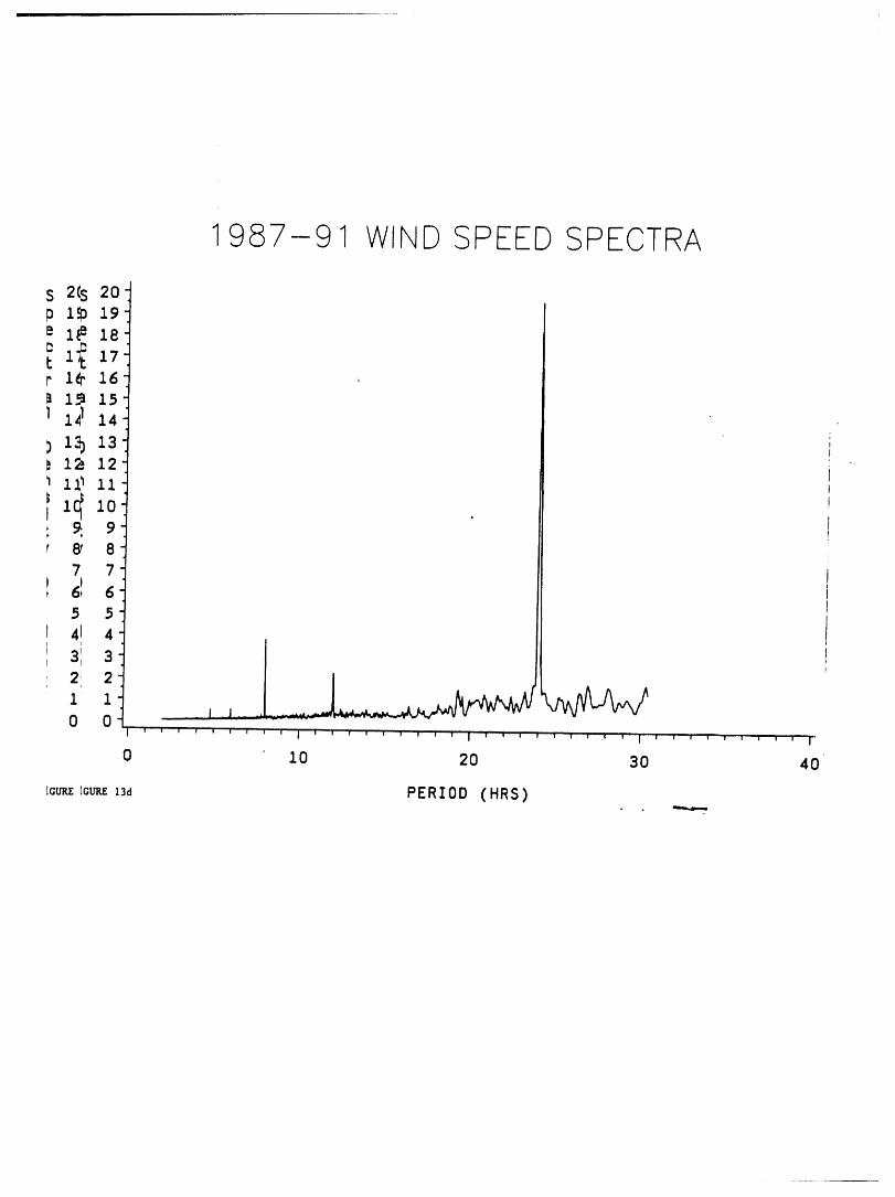
1987-91 WIND SPEED SPECTRA
s 2Cs20-1_ 19-
e i_ le-
t i_ 17r le 16-
112 14
) i% 13i_ 12
IC_ i0i: 9: 9i 8, 8
7 7
16165 5
41 4
31 3 1
1 1.0 0 .... I, - J .... . -- :-.._-._'-: Iv i i v I _ v I I I I ! ' v v i i' v I v "' ; v I .... v v v v l _' I I 'I v ! v 1 v v I I
0 10 20 30 40
iGu_zIGU_z13d PERIOD (HRS)~
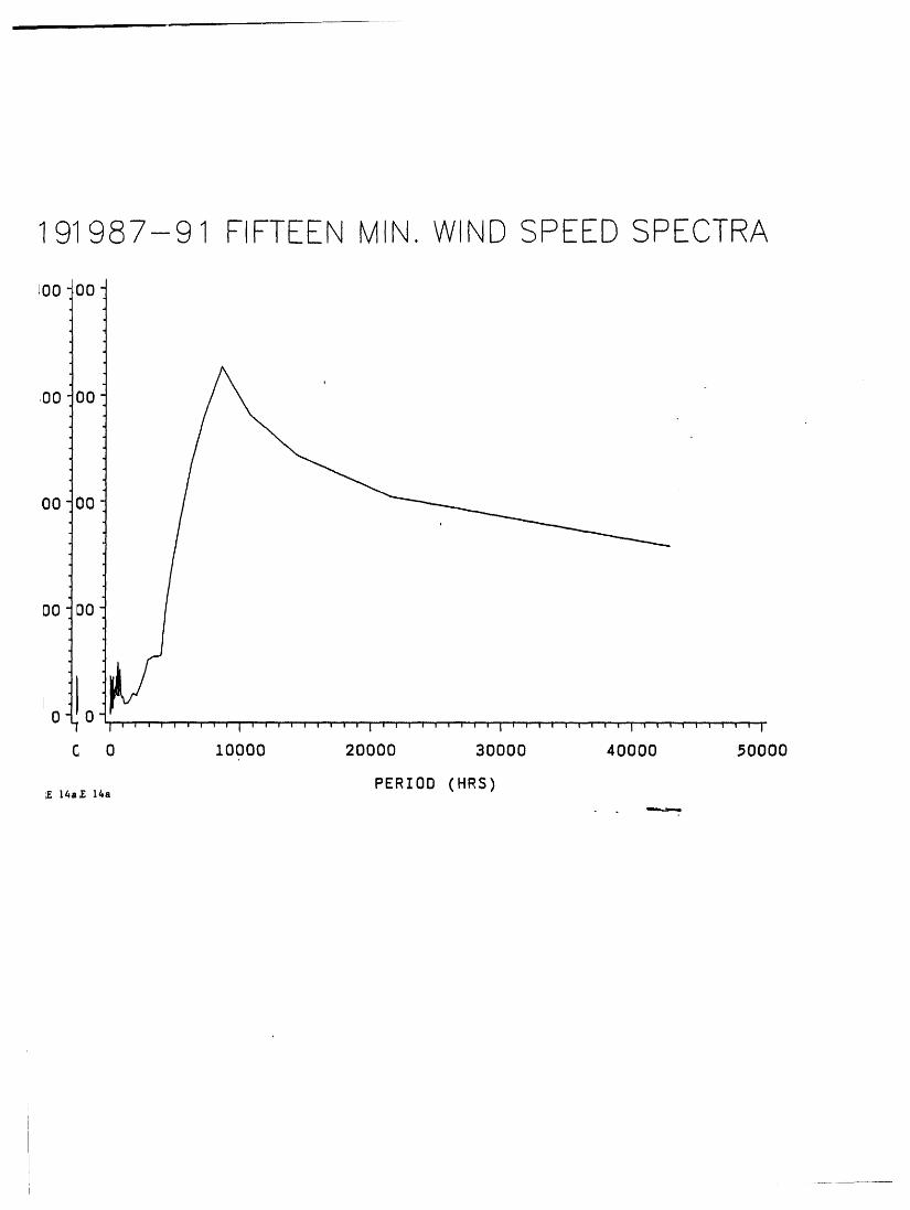
191987-91 FIFTEENMIN. WIND SPEED SPECTRA
100"00 "
O0 00"
DO DO"
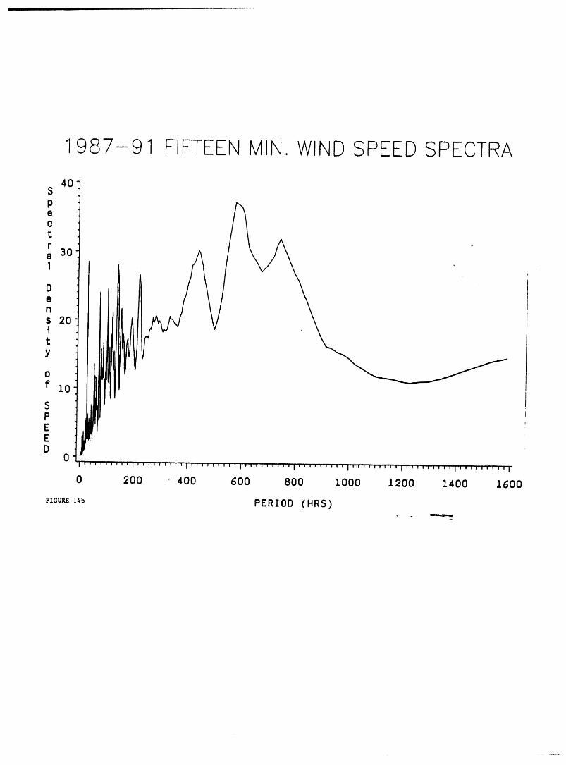
1987-91 FIFTEEN MIN. WIND SPEED SPECTRA
s 40tPectra 301
Dens 20ttY
0
f 10
SPEED
0
0 200 400 600 800 i000 1200 1400 1600
FZcU_14b PERIOD (HRS)--
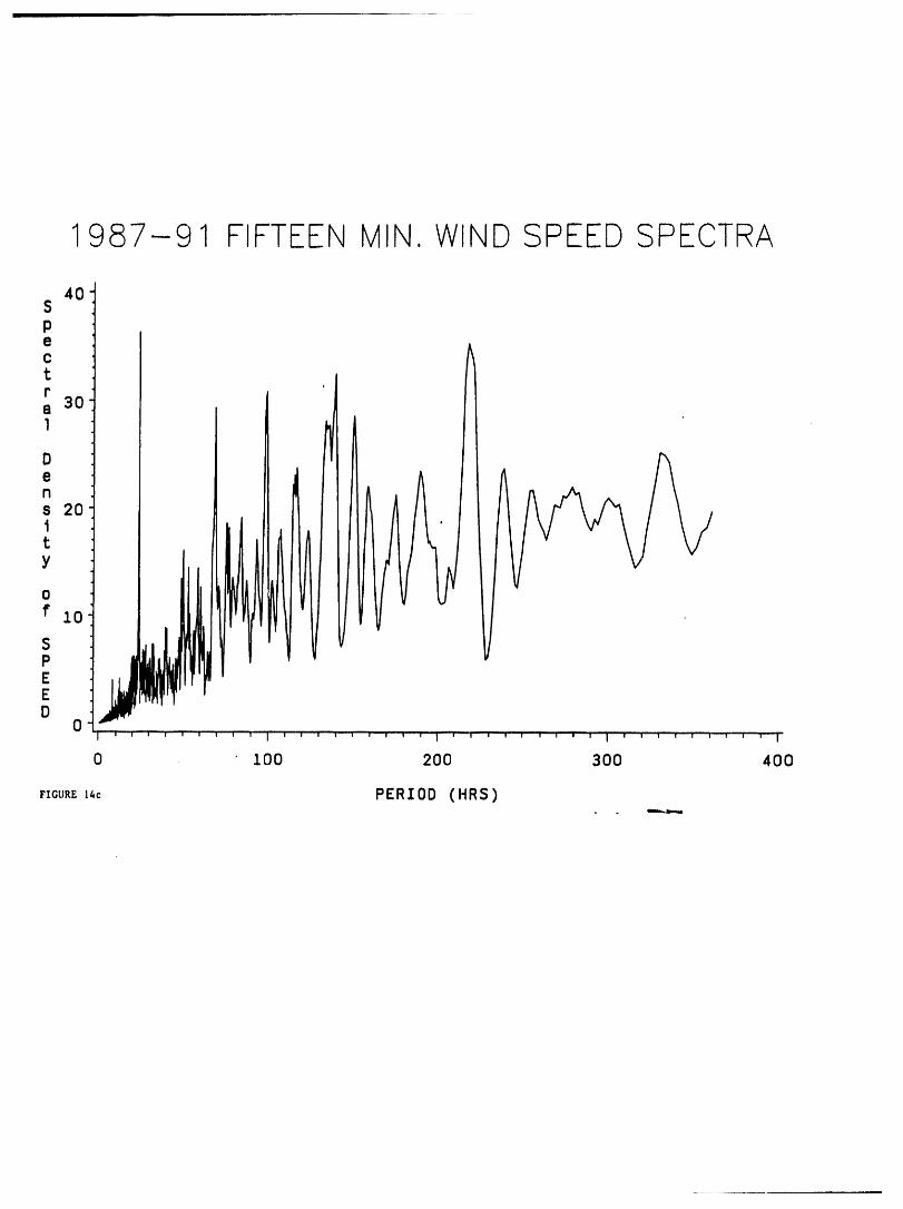
1987-91 FIFTEENMIN. WIND SPEED SPECTRA
40SPe
r
_ 3oDen
_ 2otY
D0
' ' ' ' ' ' _ ' ' I' ' ' ''' "" ' ' ' ' I ' " ' ' ' ' ' ' i i ' " '" ' '' "-' ' '.....I
0 .1.00 200 300 400
FzCUR_-14c PERIOD (HRS)
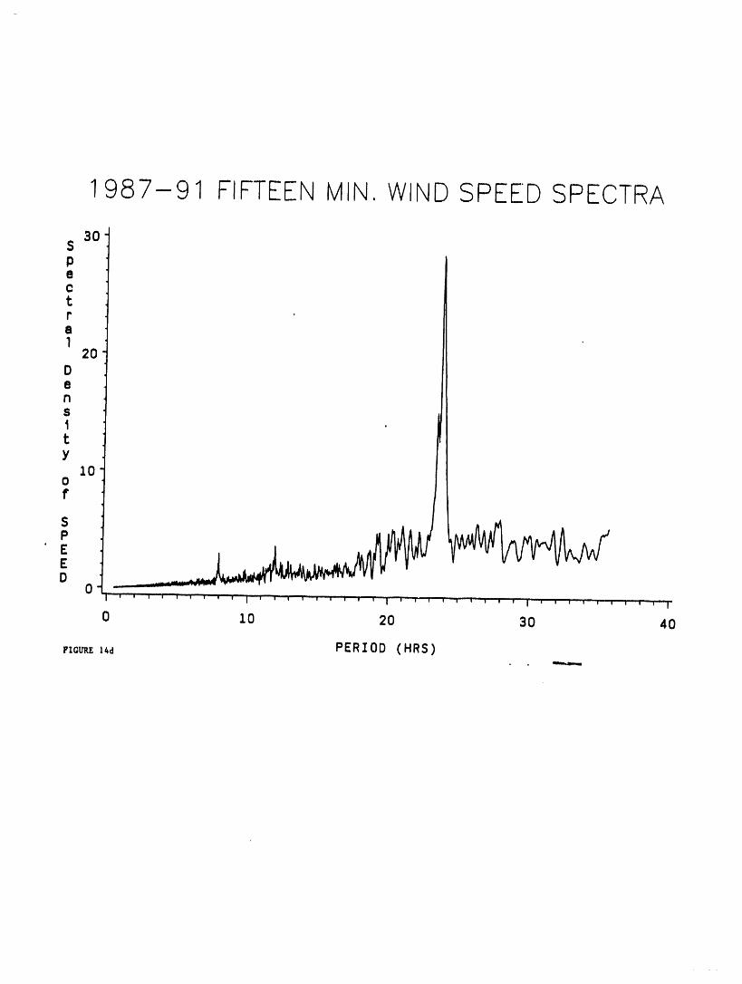
1987-91 FIFTEENMIN, WIND SPEED SPEC-IRA
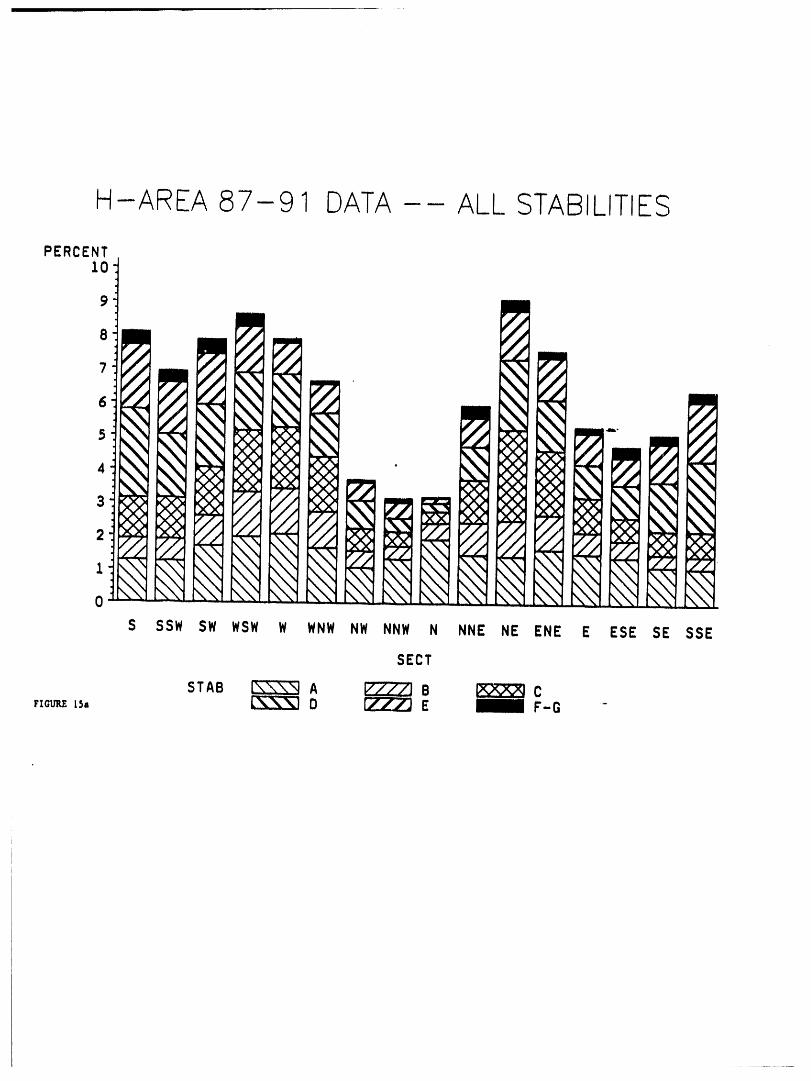
H-AREA 87-91 DATA-- ALL STABILITIES
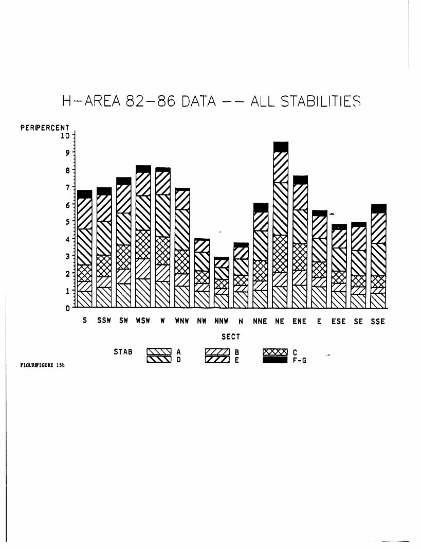
H-AREA 82-86 DATA-- ALL STABILiTIE.<:;
PERIPERCENT10
9 ////
fJ
6
4
3 N
• .
S SSW SW WSW W WNW NW NNW N NNE NE ENE E ESE SE SSE
SECT
D E _1F'-GFIGURI_IGURE15b
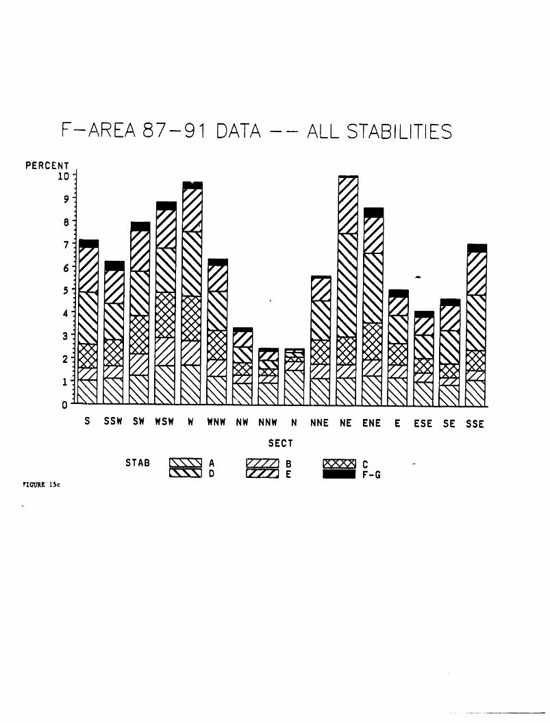
F-AREA 87-91 DATA ALL STABILITIES
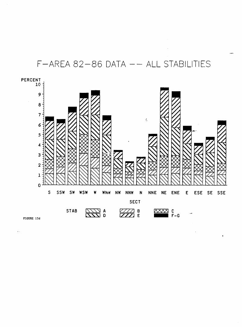
F-AREA 82-86 DATA ALL STABILITIES
°,
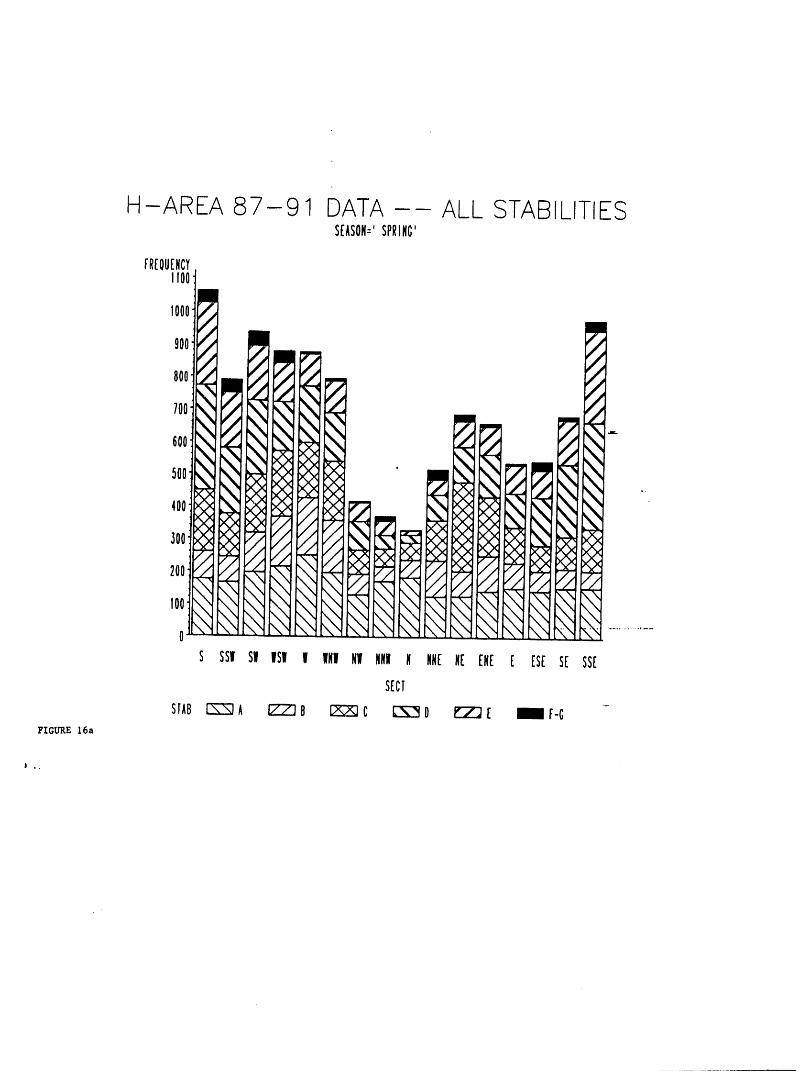
H-AREA 87-91 DATA ALL STABILITIESSEASON:'SPRING'
FREQUENCYII00
mI000,.., il900," .,' r/
800,,, ,,,, _/ F/
700_'_rJ %'_____\ _ 1 "
600_.,, .,,....%.__
%,"" %'×>'×> k-_ . _ _ _,_oo,,, "" _ x>,×>,,<× M _ _ ""_'_ >0< X> X::x K)< _% "
400 _<x >(>
,100xx ×_ -- "" _ :,Cx,<:x×:,<Kx _ x_ ××-"" .. _ )("2< _ :--)<)< - - --,-,- X[)< K_ KX
200 "- _ - - -,,--- _XX_ .. , , ..,..., _ _ ,.,.,. -,..,......___,.... _ -_
I00 .... - - " " " " ...... ,-,, ,,. . ._ . . \ \ - . -_ -_ _:._.. .............
......... ...
S SSl SI ISI 1 INI NWNN! N NN[ N[ IN[ [ ES[ S[ SS[
SECT
STAB['N-_A [7-'_B _;2_C [2_0 _E IF-G
FIGTJI_16a
|.,
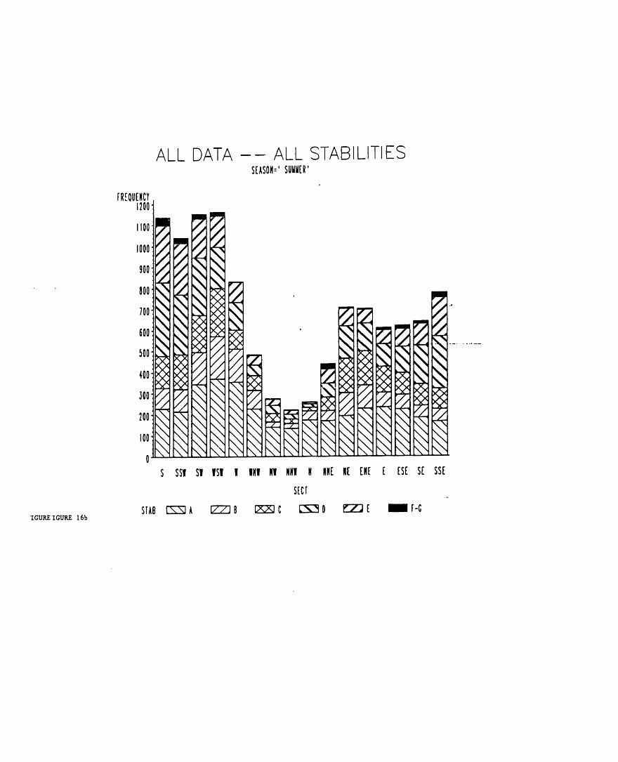
ALL DATA ALL STABILITIESS[ASON:'SUI/W[R'
FR[OU[NCY1200
I100Ill m
,ooo_ -',900_ "_f.,P
.00'°°_,,.,sx,,'"o° °°_'_ _z,,-_ _"_,--_ ,.., :£ .. _.-, ..........
500,_ "" "" _ ,o'_ _ ,¢,O ,4_ . . -- ..-. mlm:,O<>4_400 O_ <_ --
O< <._ .,,._. . _,.,__ ..-.... .,,...,.,- >43< _ >O< ..-,-.300 - -- " ..... _ ..--.--. _ ,.,.. ,O,
"-" _' O<200 ........... . ....
100........... " .......
......... j
S SSI SI ISI I INI NI NNI N MN[I1[ [N[ [ [ST ST SS[
S[CT
'IGUI_'IGUI_ 16b
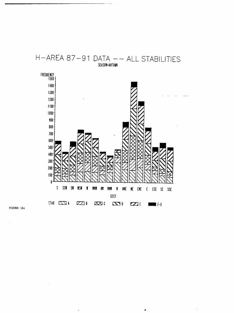
H-AREA 87-91 DATA ALL STABILITIESSEASON=AUTUMN
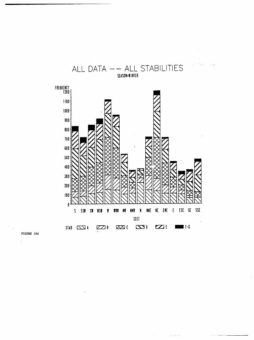
ALL DATA ALL STABILITIES .........SEASON:l/INTER
FREQUENCY120o- HI1100 i= " "
f# r,l
1000 , ,,-..-,,
,oo ,X_, X
,oo,oo .600_
. ,,300N N ._ _ " ,.-.,I,.200 _ _ `%
_/ %`% %'%
I00' " :" ×'__:- ,=,=
S SSI S! ISI I INI Nil NNI N NNEMEENE[ ESES[ SSE
SECT
STAB[_Z_IA _B I;:_::_3C I_O I_Z_][ _F-GFIGURE 16d
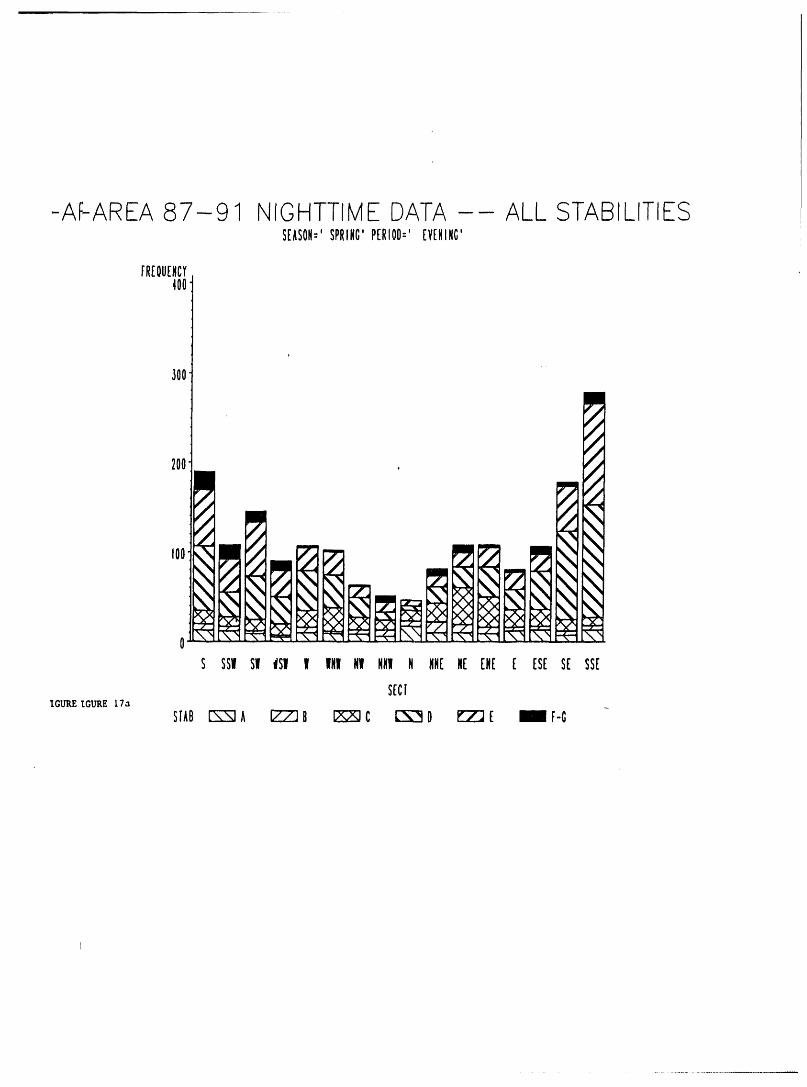
-AF-AREA87-91 NIGHTTIMEDATA ALL STABILITIESS[ASON-'SPRING'P[RIO0:'[V[NING'
FR[OU£NCY400
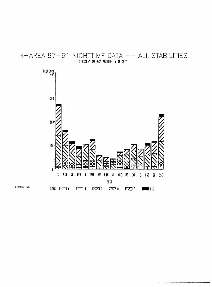
H-AREA 87-91 NIOHTTIMEDATA -- ALL STABILITIESSEASON:'SPRING'PERIO0:'MIONIGHI'
FREQUENCY400
b
300
mfJ
200 . ,, •f•
fj fJ
Cj f•
S SSI SI ISI 1 INI NI NNMN NNIr N[ [N[ [ ES[ S[ SS(
SECT
FzQueE17b SlAB_ k IZZ] B _ C _ 0 _ [ _ F-G "
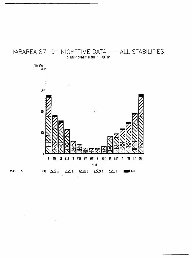
_ARAREA87-91 NIGHTTIMEDATA ALL STABILITIESS[ASON--'SUIIIt[R'P[RIOI):'[Y[ItlItG'
FREOUENCY400
300
_ fj
fJ fj _
R100 _-_ _._ ,'1 _ _.,_
X,,_ XX }'(_ KX
S SSI SI ISI I INI NI NNIIN NN[ N[ t'N[ E [S[ S[ SS[
S[CT
FzGT: 7: STAB_ A [ZZ] 8 I_ C _ 0 _ [ / F-Ct
I
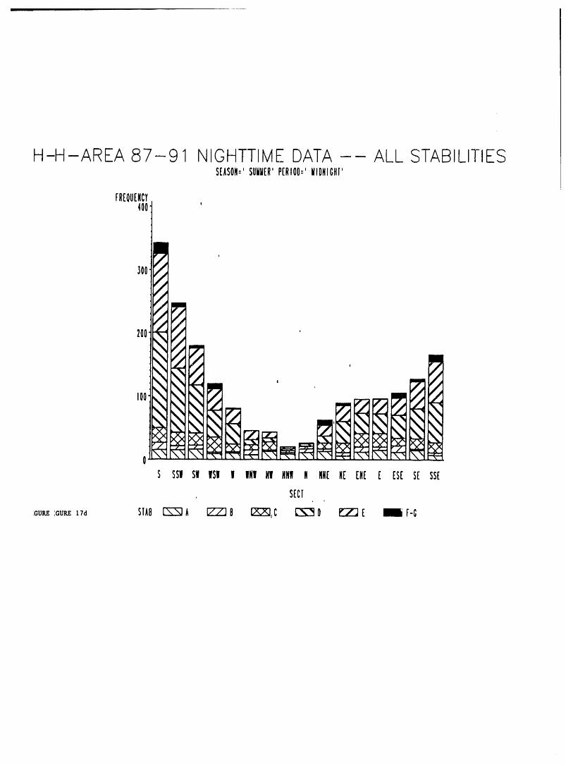
H-H-AREA 87-91 NIGHTTIMEDATA ALL STABILITIESSEASON:'SUMMER'PERIO0:'IIIDNICHI'
FREQUENCY400
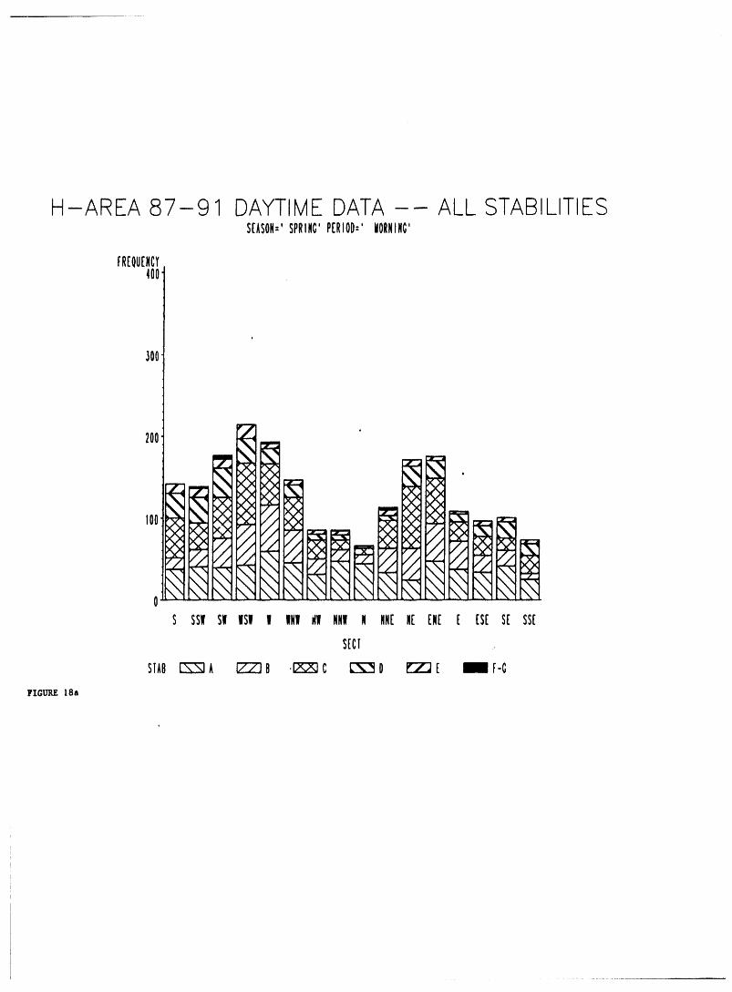
H-AREA 87-91 DAYTIMEDATA -- ALL STABILITIESSEASON:'SPRING'PERIO0='WORNING'
FREQUENCY400'
i
300
200
'000 • •
S SS! S! IS! ! IN! N! NNI l NN[ MF[N[ [ [S[ S[ SS[
SECT
STABl'N-"_:lA _B I::_::_C L-_-"_I0 l._:Z;i[ _F-C
FIGURE 18a
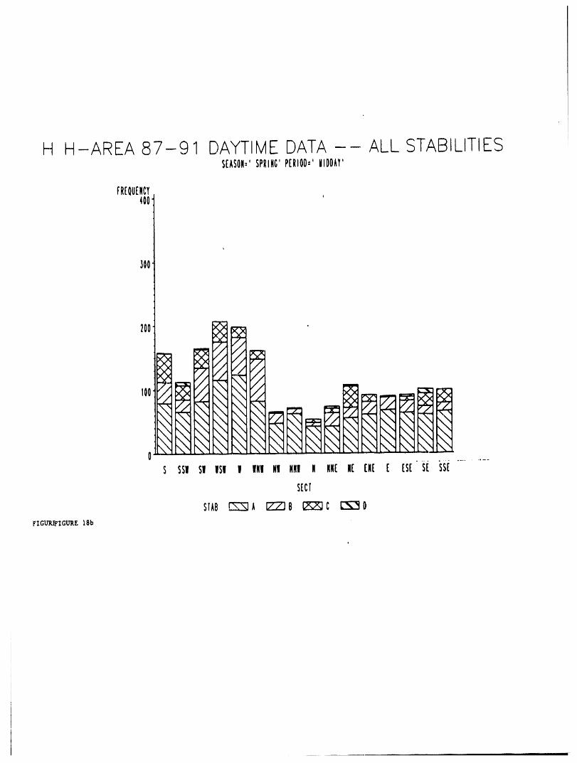
H H-AREA 87-91 DAYTIMEDATA -- ALL STABILITIESS[ASON.-'SPRING'P[RIO0='WIOOAY'
FR[OU[NCY400
,100
_oo _ _ .
/ //
, //
0 " ",7' \
s ssvsv vsv v wNvMyMptwM MN[N[ I:Ml:[ [S[S£ ssi..........S[CT
SIAl}_A IZZ]8_C [:S:SOFIGUR_IOURE ISb
i i llllJ
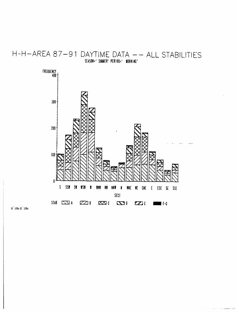
H-H-AREA 87-91 DAYTIMEDATA-- AL.L STABILITIESS[ASON='SUWW[R'P[RIO0:'IORNING'
FR[OU[NCY400
_oo 1
,oo §_f i
,.'_×_, ;; ................
.... ,.-- _< ... ,, >0_
0 "--" - "'_ "-"
S SSI SI ISl 1 IINI NI NN! N NN[N[ IN[ [ IS[ S[ SS[
SIC[
STAB["(_-'IAIZ_]B 12_C i;_]O _[ mr-cE'18c E'18c
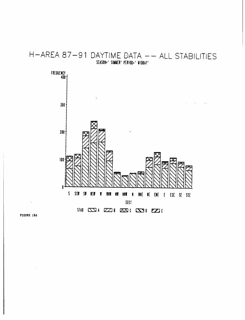
H-AREA 87-91 DAYTIMEDATA -- ALL.STABILITIESS[ASON,'SUWW[R'P[RIO0='WIOOAY'
FR[OU[NCY400
300
200 _ ,"-11 /i
// // //ii _
tO0 ;_ \\ "" _" // _ _ _'_
S SSI S'# ISI I IN! N! NNI N IN[ N[ IN[ [ IS[ S[ SS[
S[CT
SIAB[_;]$;]A_B [;]_;_;)C[:_[]P[Z;I[FIGURE 18d
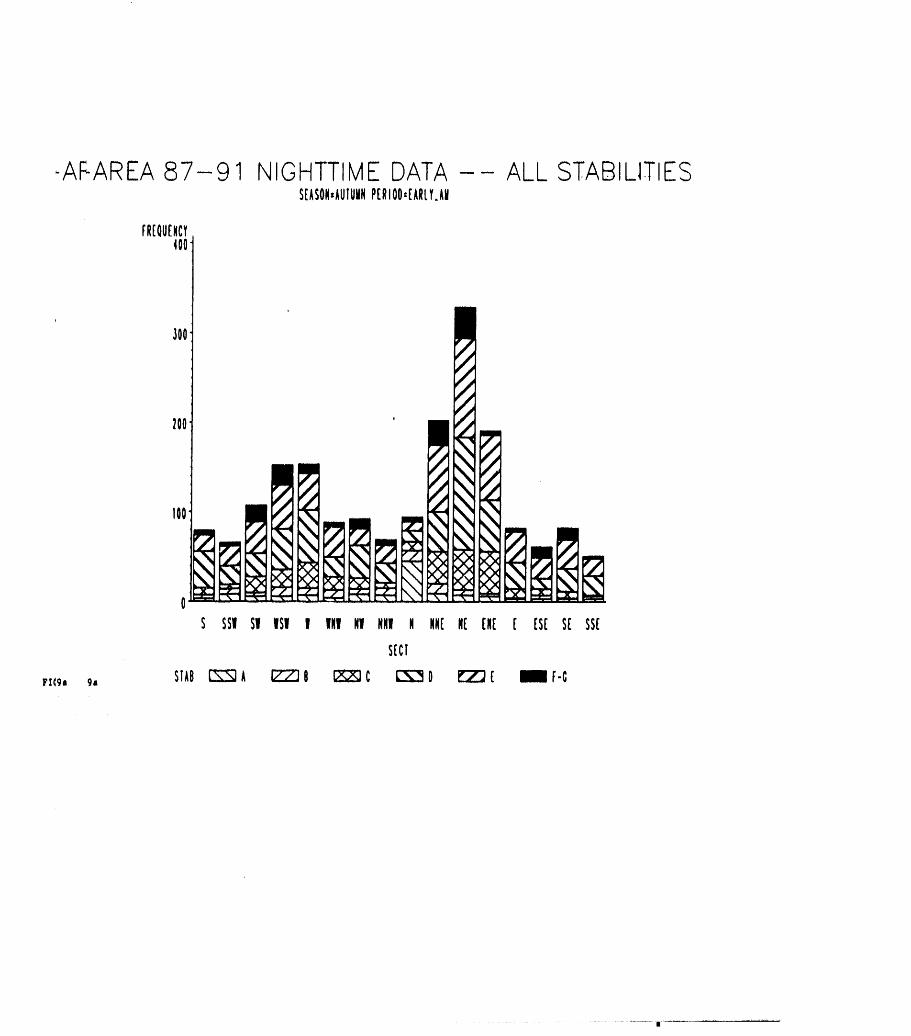
-AFAREA87-91 NIGHTTIMEDATA-- ALL STABILITIESS[ASON,AUIUWNP[RIOO,[ARLY.AW
FR[QU[NCY400
..... •...........................al
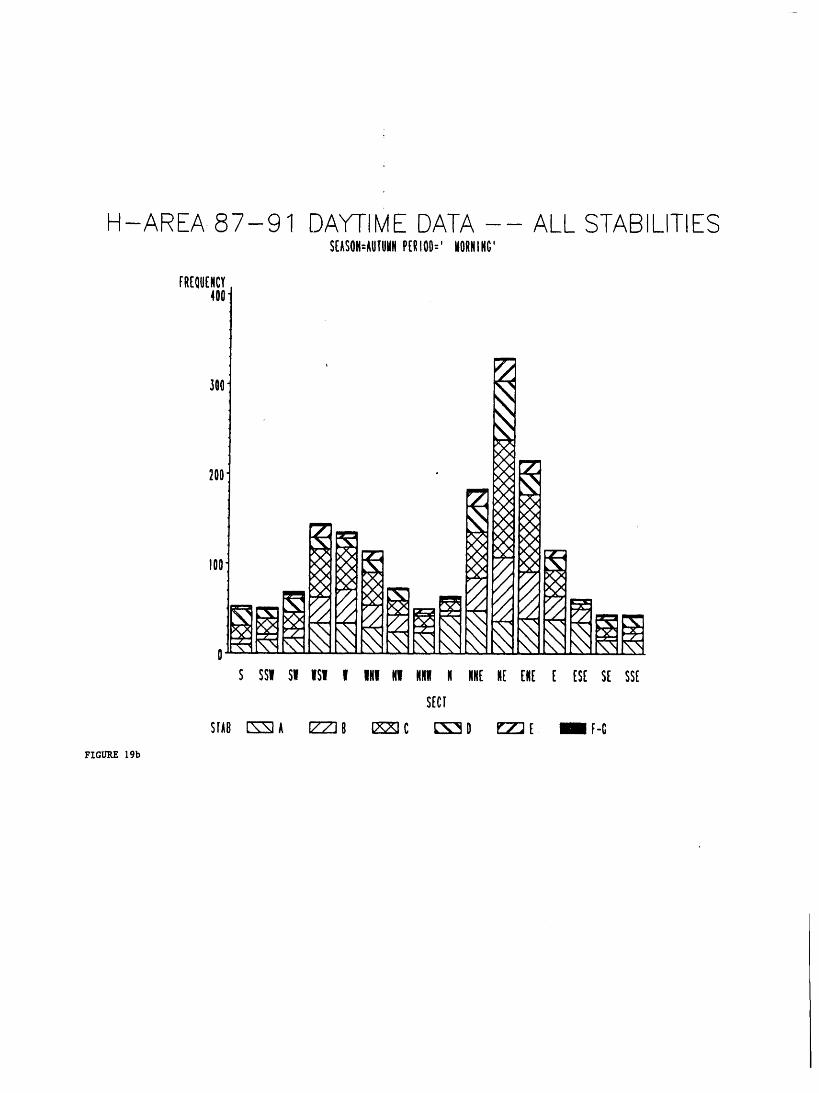
H-AREA 87-91 DAYTIMEDATA ALL STABILITIESS[ASON=AUTUUHPERIO0:'IIORNING'
FREQUENCY400
m_jpm
300
X
.k'_ X_ _. 4 .....
x[)_x._ x)< " "
o IN",i . . • •
S SS! Stl tlSI tl tlNtl Nil NNWN NN[ N[ ENE[ [S[ S[ SSE
SECT
SIA8 ['_'_ A [7-/]8 [_] C L'_-_D I_'J_ E NF-G
FIGURE 19b
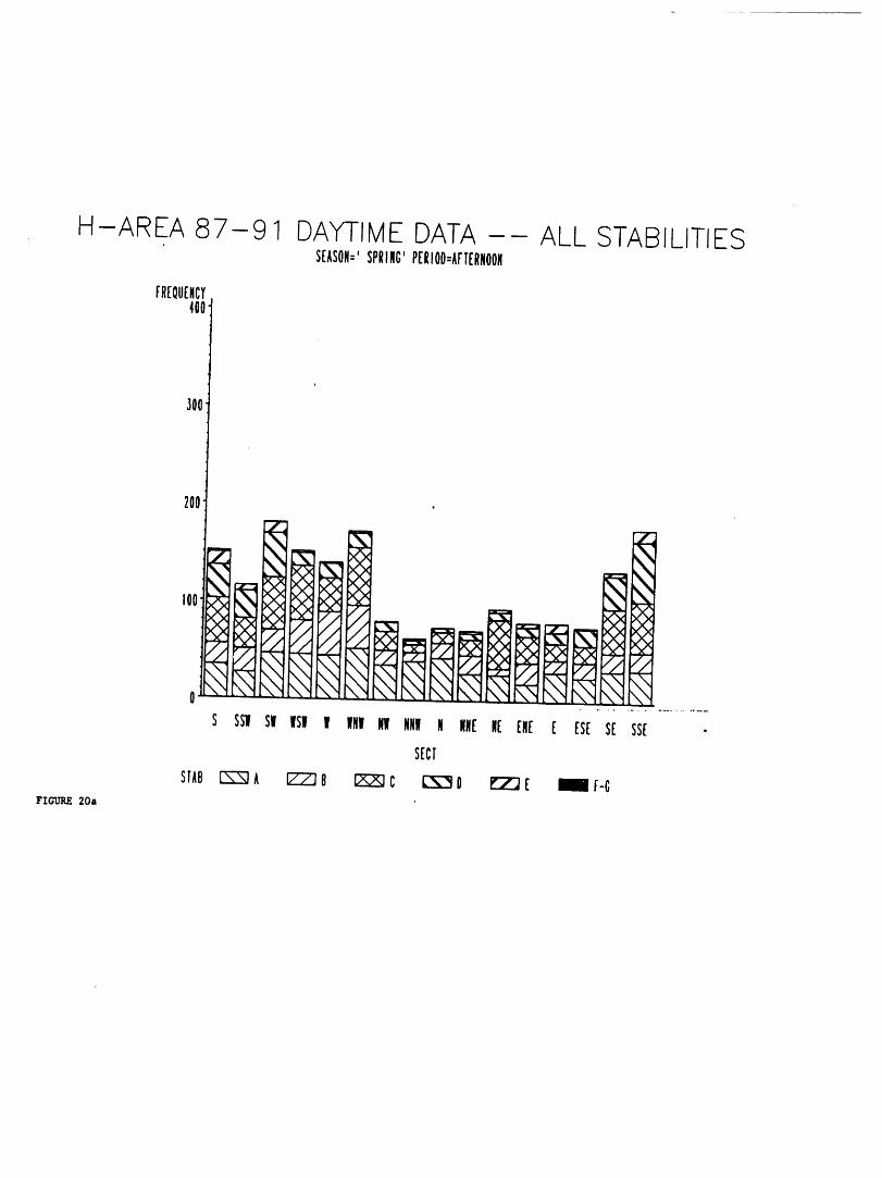
H-AREA 87-91 DAYTIMEDATA ALL STABILITIESSEASON =' SPRING' P[RIOO"AFT(RNOON
FREQUENCY400
300
200
XX >0_ :<x "-_
"%. %. '%. _.
\\....
S SSl SI ISI I IIININI NNI N IIN( ]( [N[ E [S( S[ SS(
SECT
FIGURE 20a
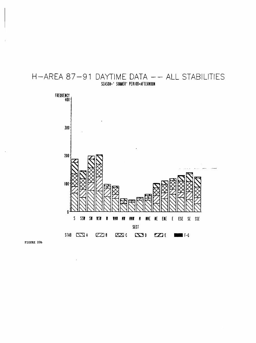
H-AREA 87-91 DAYTIMEDATA ALL STABILITIESS[ASON='SUWW[R'P[RIOO=AFI[RNOON
FR[OU[NCY400
i
300
200 __X_, N ..................
. .- - -,_,,. _ ,.,, \,, i
....... i |
S SSI SI ISI I I111 II Nil I Nil I[ [l[ [ IS[ S[ SS[
S[Cl
SlAB [_-"_A _B _C [_-'_O _[ _F-G
FIGIJItE20b
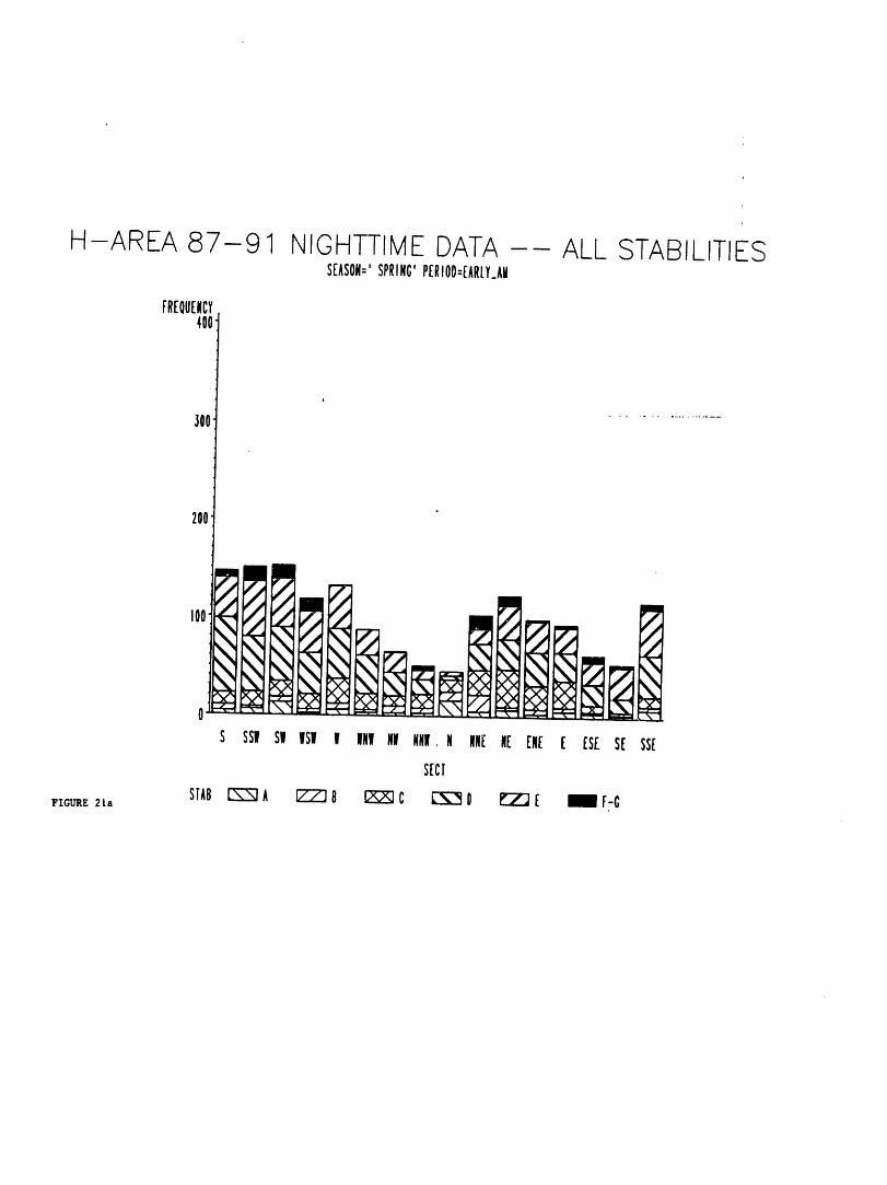
H-AREA 87-91 NIOHTTIMEDATA ALL STABILITIESSEASON='SPRING'P[RIOO=[ARIY_AW
FREOUEMCY400'
300
200
w
r_ M
. Illi_Pl II_lUUil fJ
0 +:ii-x+]L"% 1; :"- :" -- :" -" :L /" J'[ /" +" " " '[\i[ "- _'_ "_ ]_L X_]"
S SS! S! IISI! fiN!N! 1111,I llI[l[ El[ [ [S[ S[ SS[
SECF
STABI"_-"_3A _B [X_C _O _E mF-CFIGURE 2la
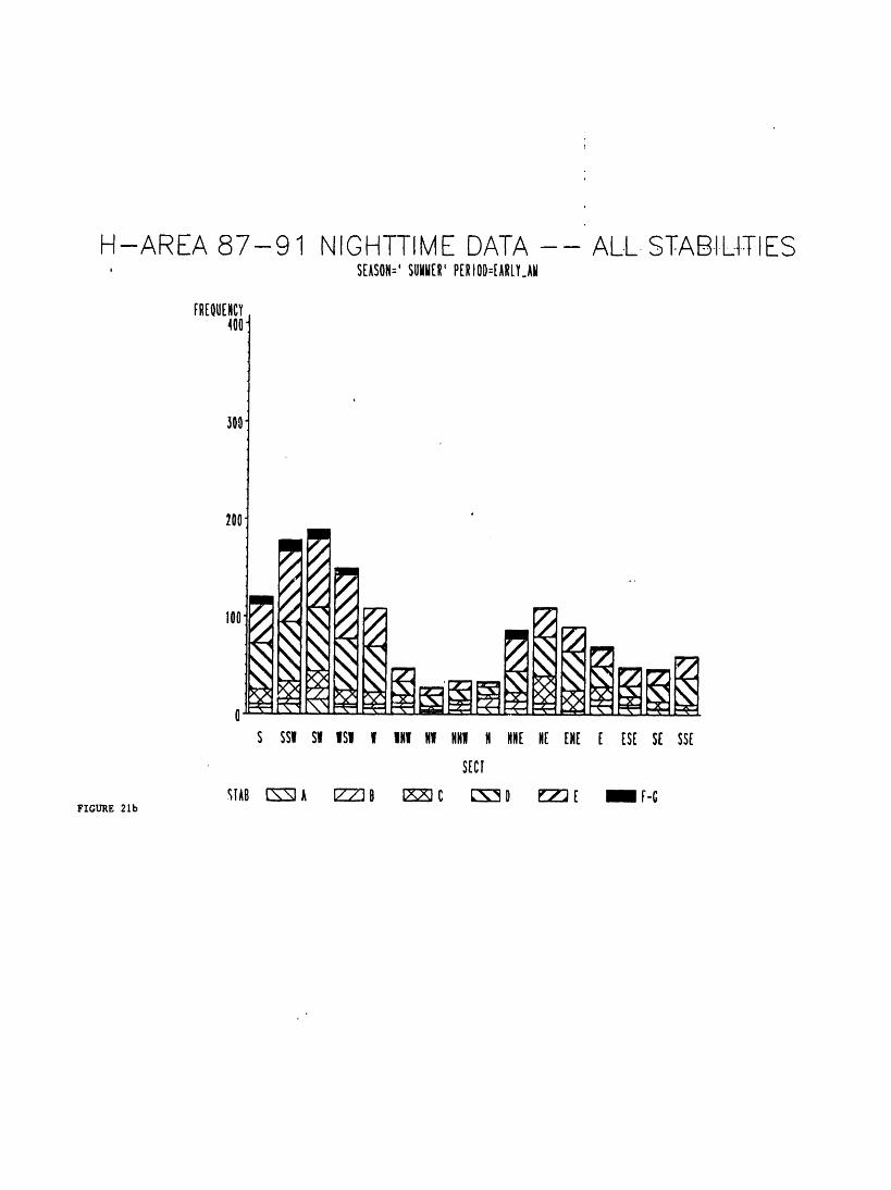
H-AREA 87-91 NIOHTTIME DATA ALL.STAB.ILITIES, SEASON:'SUIIII[It'PERIOI)=[AIILY.Ail
FREQUENCY400
i
300
200
mrj
rj _j
I00 ,,.,, ,-.,
0 =_ :::L:::S SSWSI ISI I INI Nil NN! N NNEHI [HE [ IS[ S[ SS[
SEC[
_TABL'_-'_T3A[ZZ]B [;s_::::s_]C[_[]]I)_[ NF-CFIOUI_I_ 21b
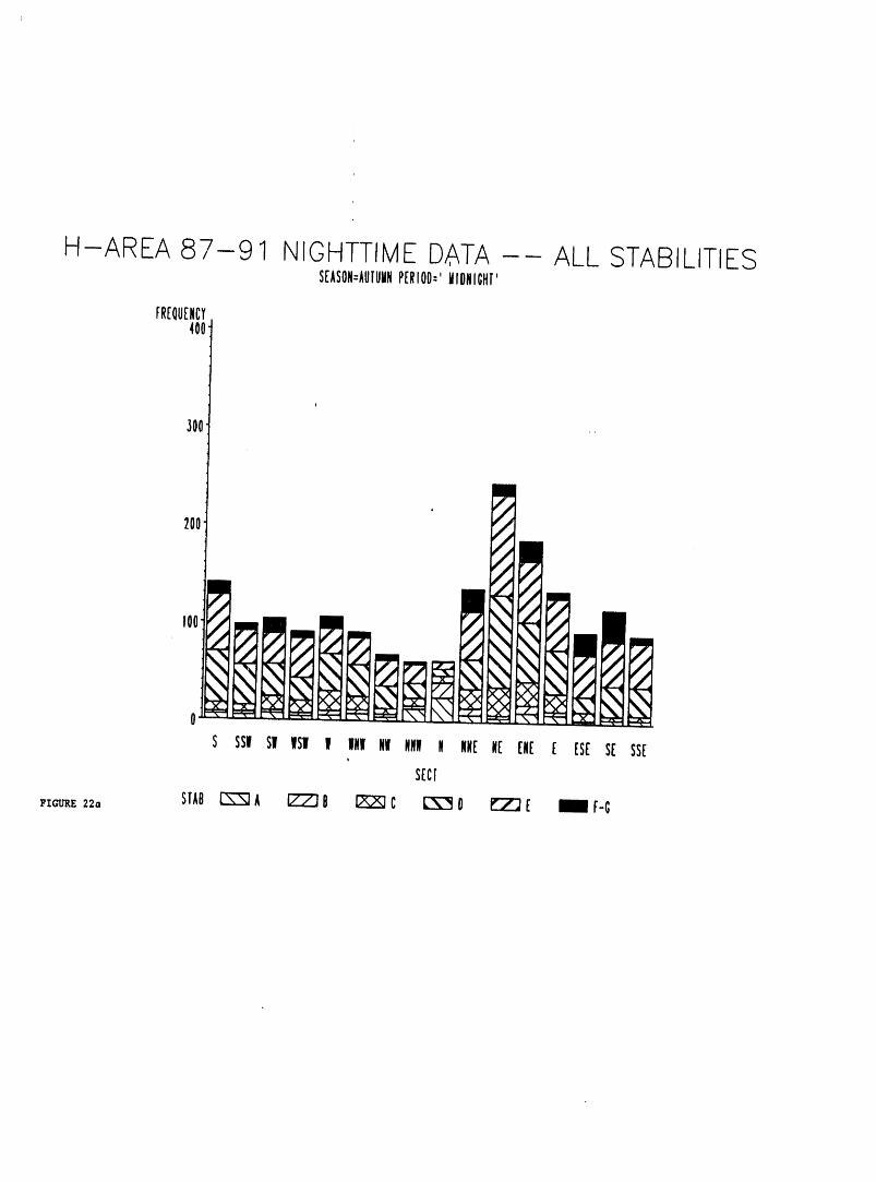
H-AREA 87-91 NIOHTTIMEDATA ALL STABILITIESSEASON:AUTUIINPERIO0='ilIONIGH['
FREQUENCY400"
J
200
,oo t_o t
S SS! SII IS! ! IINWNWNNWN NNEN[ [N[ [ [ST SE SSESEC[
FzG_n_E22. STAB_ A _ B _ C _ O _ E N F-O
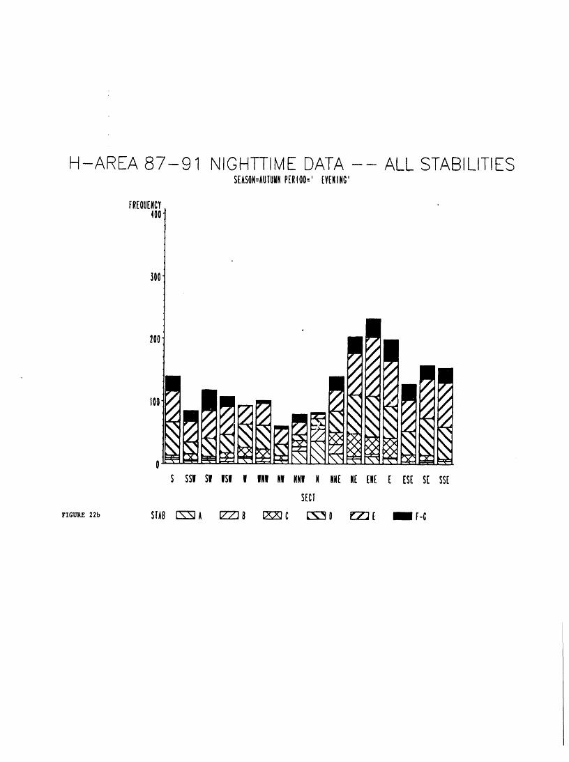
H-AREA 87-91 NIGHTTIMEDATA ALL STABILITIESSEASON-AUTUQMPERIO0='EVENING'
FREOUFNCY400
i
300
200
I00̧
0
S SSIISI ISI I INn NilNNIIN MNE N( [ME E (S[S[ SSE
SECT
FIGURE22b STABr_ A C_ n C_ C _ O e_ E m r-c
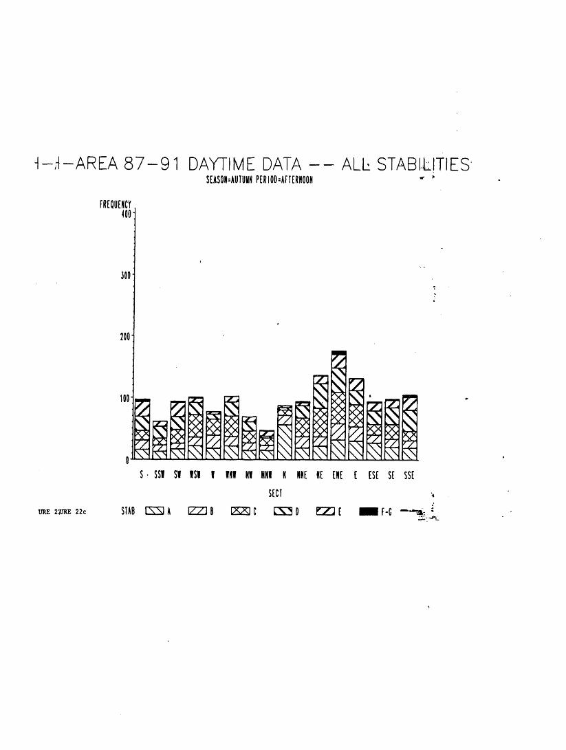
-t-,-t-AREA 87-91 DAYTIMEDATA ALl, STABI.LITIESSEASON-AUTUQNPERIOD:AFTERNOON " : "
FREOUENCY100
i
3OO
200
m
mmm,glm
", . ,
S. SSI Sl ISI I INI NI NN! N NNElie ENE [ [SE St SSE
SECT _
ve,z 2,'_22_ STAB[_Z_3A [7"7]0 [2_ZIC l-%--'_lO[Z_IE _F-G _ _
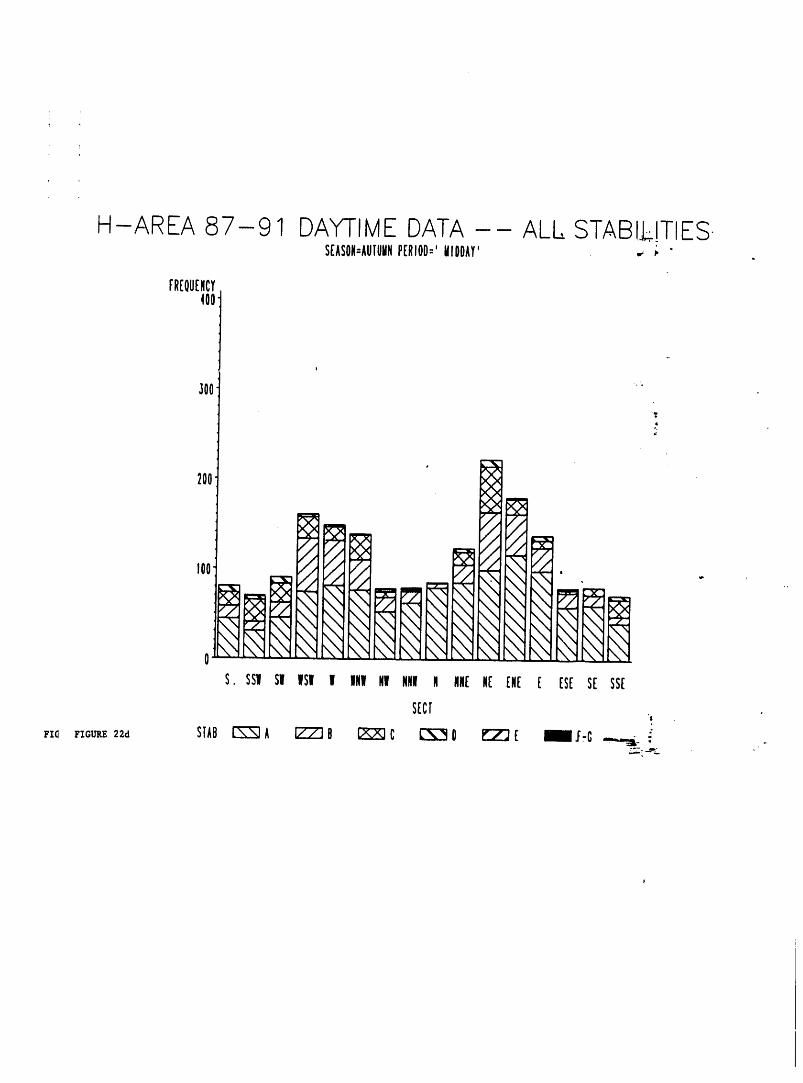
H-AREA 87-91 DAYTIMEDATA ALL STAB!L.,!TIES-SEASON=AUTUIINPERIOD='UlDDAY' -' _' " .
i
300
o,
200 _3x
I00 / j L/J /j _ \% -.,r,..-- • ,,,fJ /./ -_._ %.% %% ,
,..,'"r_,- _ _'-",., --%% \%.
%.% %%
%% %%
%% \\
, , .
S. SSI SI ISI I Ill Nil NNWIt NN[ N[ (N( ( l[S( S[ SS[
S[Cf .,
zzct ZZGU_e._2ad STAB_ A _ 8 _ C _ 0 _ [ _ I_--G--"'a- "
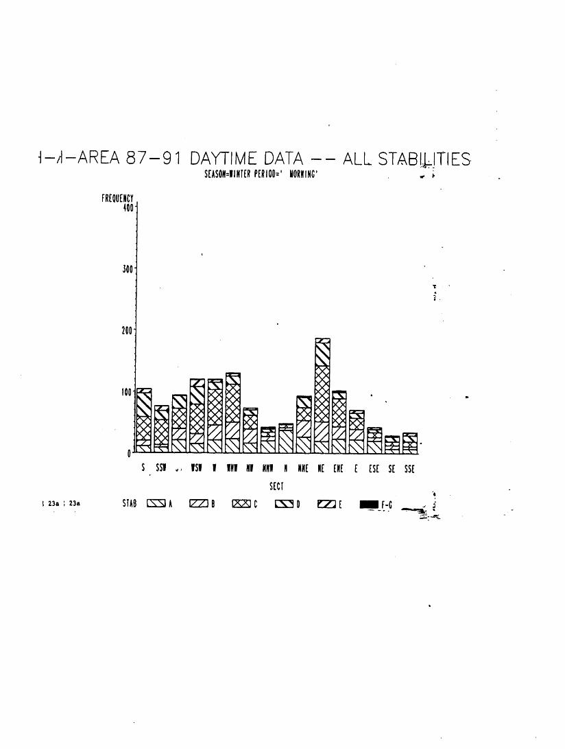
_-_t-AREA 87-91 DAYTIMEDATA ALL STAB!.L!TIES.S[ASON=IINT(RP[RIO0:'WORNING' ., _,
FREQUENCY400"
200
X[)c }4)_ _<)< , "
_']x }4X _:X
-0 \",t t'_'-'f _\1
S SS! ,,, ISI I WNINIl NNII N NN[ II[ [N[ [ [ST ST SS[
S[CT"4
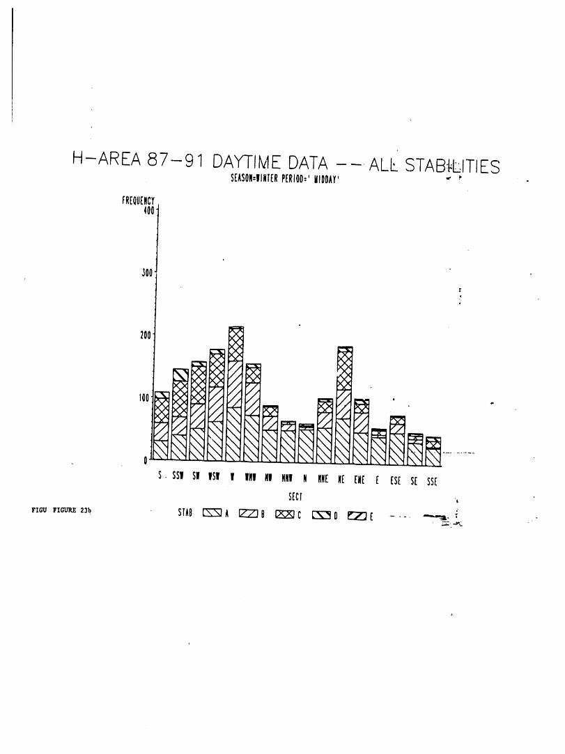
H-AREA 87-91 DAYTIMEDATA--. ALL STAB_.L-ITIESS[ASON=IINTERPERIO0='WIOOAY' " _' .
FR[QU[NCY400
200
S. SSI SI ISI I INI NI NNII N NN[ N[ [N[ [ [S[ S[ SS[
SECF .,
Fz_ FZG_n_2)b STAB_A _B [_C _0 l_[ ..... _. 6s T
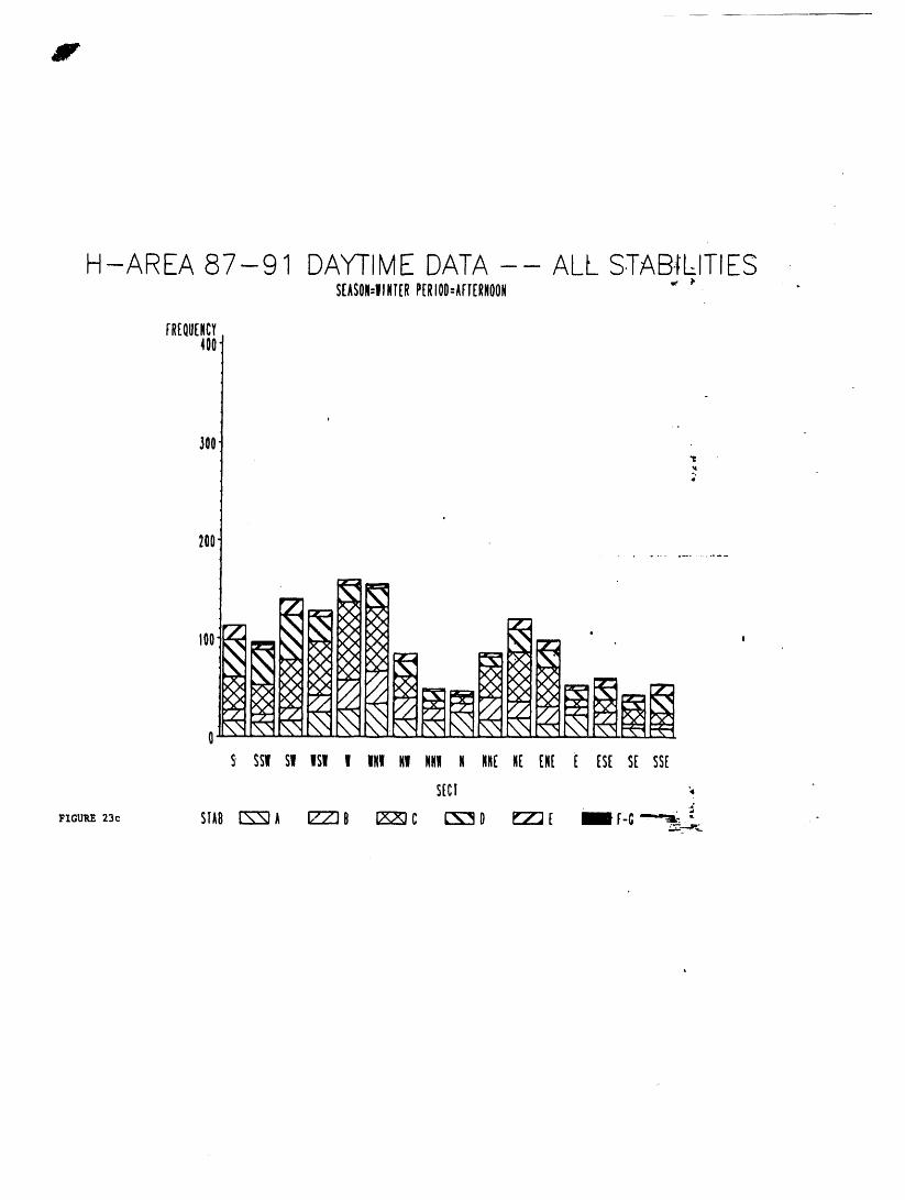
H- AREA 87- 91 DAYTIME DATA ALL S.TAB.IL-ITIESSEASON=WINTERP[RIOIi--AFT[RNOON " _' "
FRI:QUCNCY400
300
_°
i
200
-IS" SSI SI ISI I IKl NI NN! N Mitt:N[ IN[ [ ES[ S[ SSE
SECT "_._"
FZGU_23,_ STAB_ A _ B _ C _ 0 _ E _ F-G_: __,"_, "-"
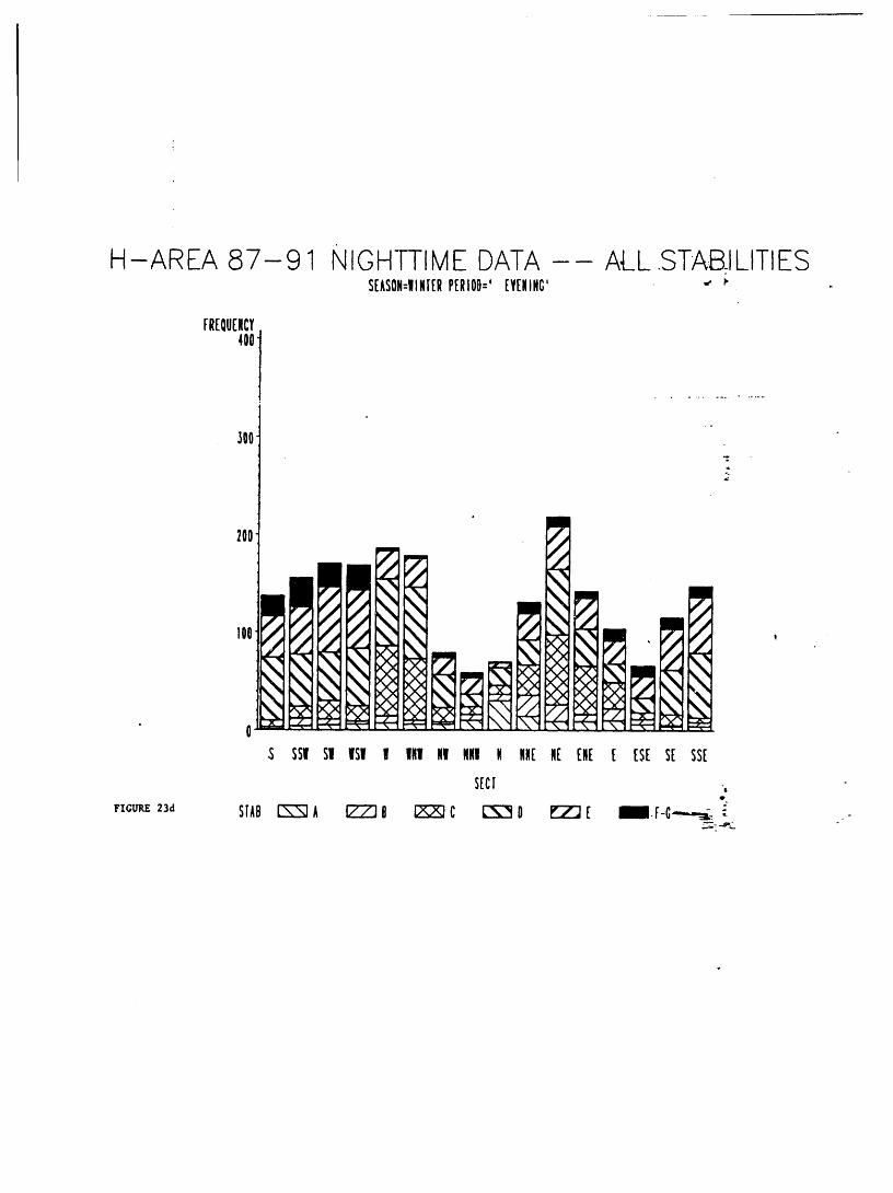
H-AREA 87-91 NIGHTTIMEDATA ALL,STABILITIESSE,_SON=IINI[RPERIOD='EYEItlNG' "_ _" -
F'EOUEIII! .................i
• °
300
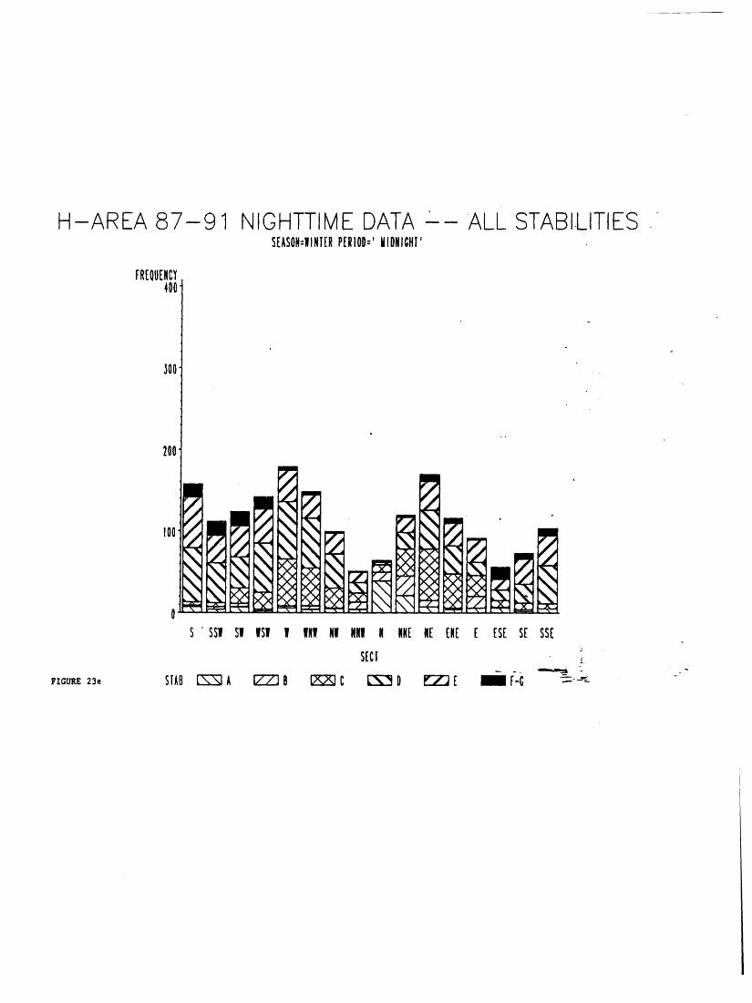
H-AREA 87-91 NIGHTTIMEDATA ALL STABILITIESS[ASON=IINT[RP[RIOD='WIDNIGHI'
FE[OUENCY400
300
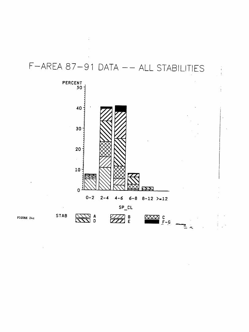
F-AREA 87-91 DATA ALL STABILITIES
PERCENT50"
40 'I/// I/_',f// t//i_. _. -4 t/i\\\ I/.,
30 \\_ i/t\\\ .sl
20 _,_
10 XXX.. ,. X>O<
0 """ ....... _ ....
0-2 2-4 4-6 6-8 8-12 >=12
SP CL
STAB L\\'<,N A [7777] B _ CFIGUI_24c _ D 1777] E _ F-G '
. . _ , '-
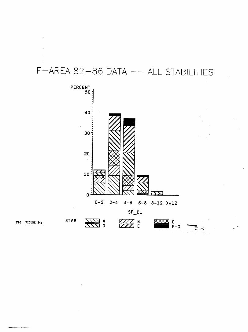
F-AREA 82-86 DATA ALL STABILITIES
PERCENT50-
40 '
2O
10 _ /,';' \-
o - <<\
0-2 2-4 4-6 6-B 8-12 >=12
SP CL
FIG FIGURE24d STAB L\\\'_l A V"///J B _ CC\\\l D _ E _ F-G
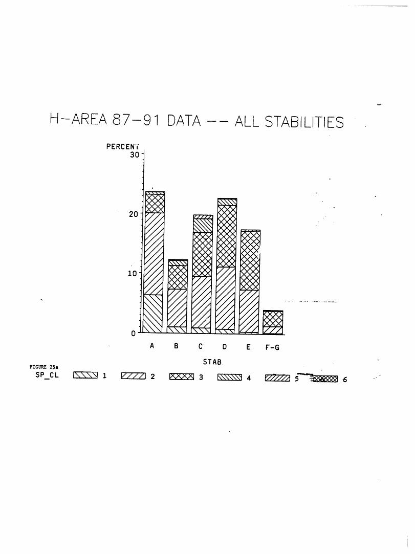
H-AREA 87-91 DATA ALL STABILITIES
PERCEN(30
i ,. .
20 .... ,
...... I
NNNMMNNNNNNN
10 --- _._
" -" --" ,: /". /
/
! 'N/
A B C D E F-G
STAB,FIGURE 25a
SP CL [\\\"4 1 [7777] 2 _ 3 _ 4 _ 5"--z-_ .6 -
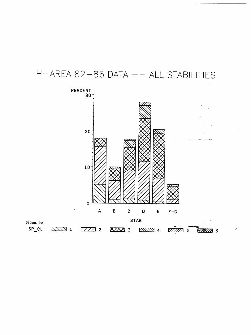
H-AREA 82-86 DATA-- ALL STABILITIES
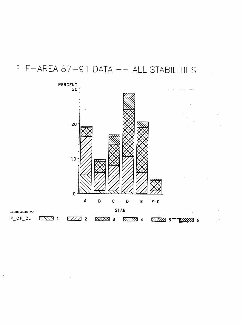
F F-AREA 87-91 DATA ALL STABILITIES
PERCENT30 ...........
f/I/ •
_'.
, Nx_XX_XXN
20 >00_ ,._'-_',.:"><X_x><X><
-- -- .,' _ _X]X
--- _,_f J J
/ / !
j- f j-
i0 _ /- -/
/ /.,_,_ / /
/ /
'" " ."/.40 " " " _-_-\ • - •
A B C D E F-G
_Icmu_Icmu_2sc STAB
IP_CIP_CL _ 1 V///] 2 [X_ 3 t,,\\\\\"14 V/7/,"A 5 _ 6 -
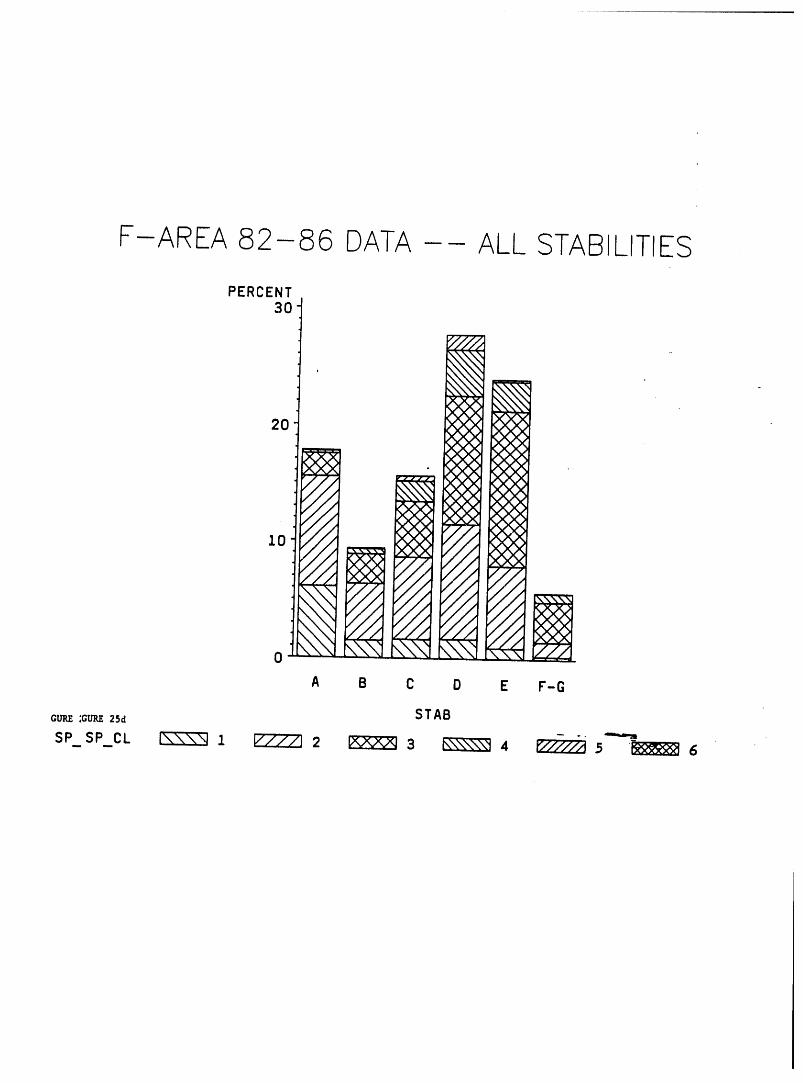
F-AREA 82-86 DATA-- ALL STABILITIESPERCENT
30'
20
•_ ,,• _ _ _
,///
.///
//./
///
10 .'_'," ""i i
i i i
///
, I/ -- ,,II --
' I//I " " "
0 X N _ ..- {-- , .....
A B C D E F-G
Gum_:Gum_zsd STAB
sP sP CL r,,\\_ 1 _ 2 _ 3 _,\\\\\'14 _5 "_ 6
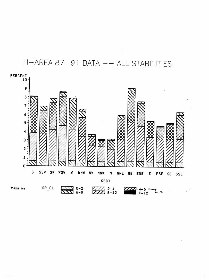
H-AREA 87-91 DATA ALL STABILITIES
PERCENT
7 _ _\
3 " / ,, //A i A ,'J //.j r/./!
2"_ ''" t i v / - - - ] I .,,a ,'2 " / " '" / " "" / ' /I ,'
.... ,, - -. _ -,_ _ _ - .......... _
S SSW SW WSW W WNW NW NNW N NNE NE ENE E ESE SE SSE
SECT
FZOURX26,, SP CL L_\'_"CI 0-2 P:'-/77] 2-4 _ 4-6 _ .- L'_._I 6-8 li//J 8-12 _ >=.1.2 _ ""
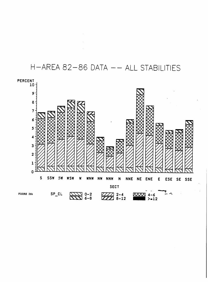
H-AREA 82-86 DATA ALL STABILITIES
PERCENT10
9
- -/ . -/2 ' - -/ - -/_ _ _ /
. . . - -/ . -/
..., ,// --/1 I
{':• _ __ _ __ .... _ - __ ..... _ _ _ _ _ --0 - --- - --_- - -- - -- - -- - -" _' -
S SSW SW WSW W WNW NW NNW N NNE NE ENE E ESE SE SSE
SECT
_Io_ z6b SP CL _\\N 0-2 V///J 2-4 _ 4-6 --_- _ 6-8 r777J8-12 _ >=12
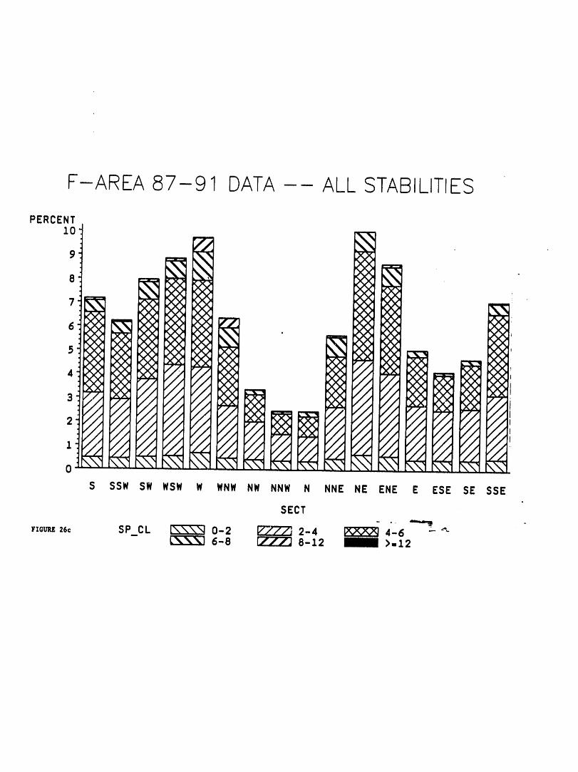
F-AREA 87-91 DATA ALL STABILITIES
PERCENT10
8 %=_ \%. _)0<)CK%.\ )CK
6 _ 77 xx <x>
5 _ %\ XX ..... <><><X> X_ "_<X> i _ <X>
4)<) <X> " 4X> _<X)'.,_,_ 4X> "" OO ,.---, <X) 4X), ,=,,._
3 _ -- <DO,_ <)4)
2 -- /_.• - . {
i- ,i _ _ _ _
0 ....... \\ -" ................
S SSW SW WSW W WNW NW NNW N NNE NE ENE E ESE SE SSE
SECT
FZOUF,Z 26c SP CL _ 0-2 _ 2-4 _ 4-6 "'_- _ 6-8 r777] 8-12 _ >=12
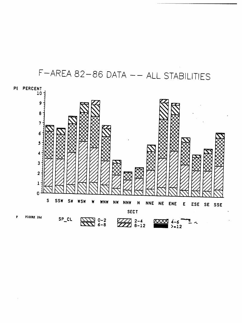
F-AREA 82-86 DATA-- ALL STABILITIES
Pt PERCENT10-
8 \_ \_
N
S _
422 "'/ '
// / _ , /-/- / ,, _ /- _ _ /
_ _/ _ _ /- _ _ /
../_¢.._._// , , _ ,
S SSW SW WSW W WNW NW NNW N NNE NE ENE E ZSE SE SSE
SECT
F l,za_ 26d SP CL [\"i\_ 0-2 _777] 2-4 _ 4-6Lk%=_l 6-8 [2l/j 8-12 _ )112
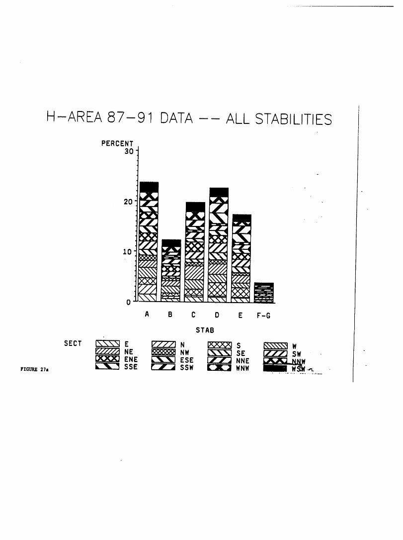
H-AREA 87-91 DATA ALL STABILITIES
PERCENT
o
20
10
0
A B C D E F-G
STAB
SECT [\\\_ E v//_;_'J N _ S _\\\\\_1 WBE _ NW _ SE _ $WERE _ ESE _ NNE
rzouP,E 27a _ SSE _ SSW _ WNW ._.• , .o .... o ........ .__
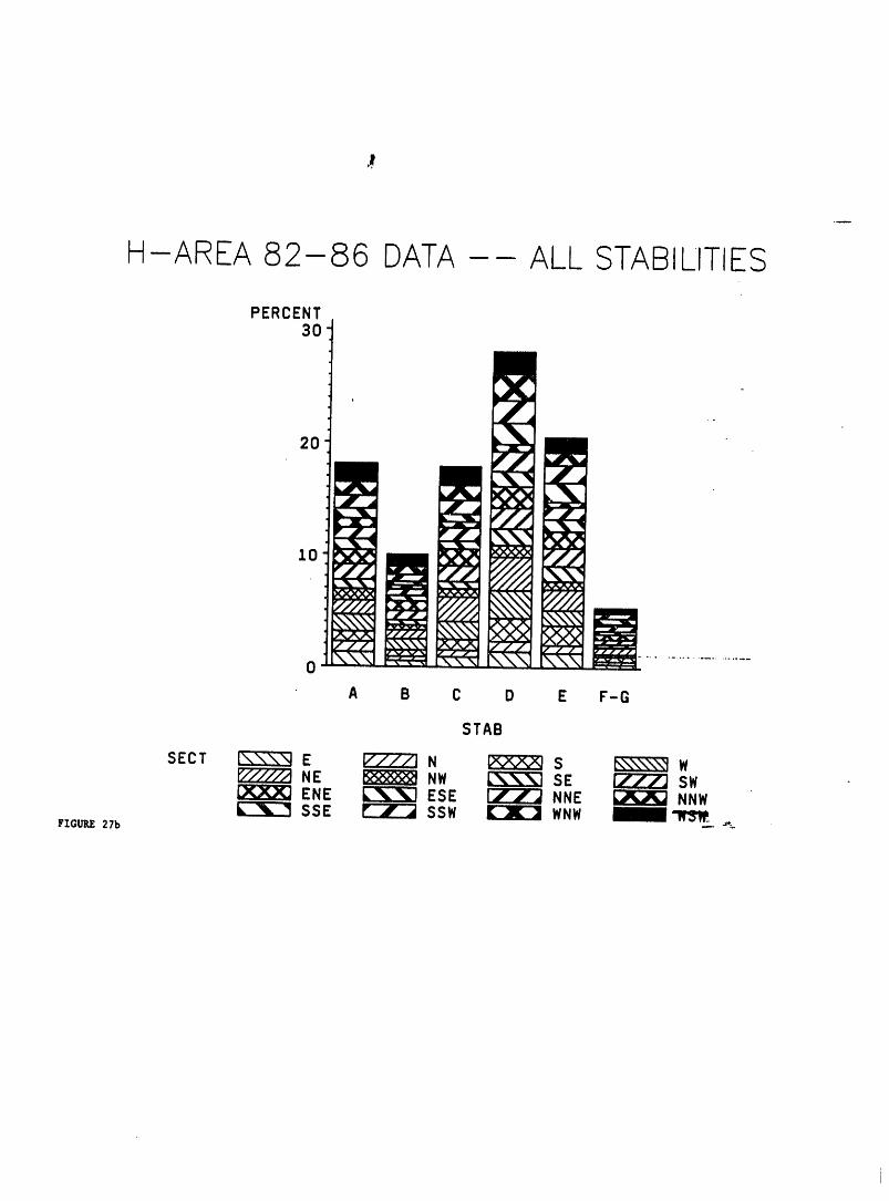
H-AREA 82-86 DATA ALL STABILITIES
PERCENT30
2O
10
0
A B C D E F-G
STAB
SECT _E _N w,vY,P<,,xjs _\\\\\_WNE _ NW _ SE [L/_LJ SWENE _ ESE _ NNE _ NNWSSE _ $SW _ WNW ___,.
FIG_ 27b
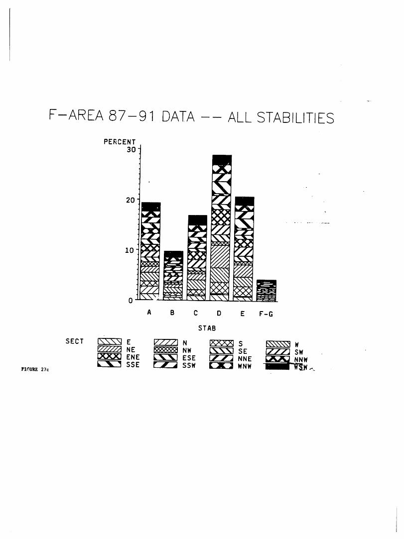
F- AREA 87- 9 1 DATA ALL STABILITIES
PERCENT3O
20
10
0
A B C D E F-G
STAB
SECT I\\\_ E {7777] N _ S _WNE _ NW _ SE [777] SWENE _ ESE _ NNE I___,NNWSSE _ SSW _ WNW __
FIC_RE 27c
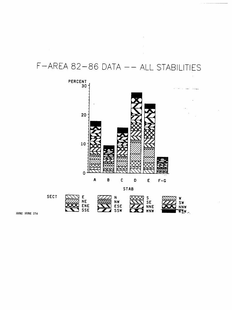
F-AREA 82-86 DATA ALL STABILITIES
PERCENT
3O t ..............
,°
20
10
0
A B C D E F-G
STAB
SECT ['_\\NI E I/_/_Z.,_] N _ S K\\\\\'IWr_/___/_/_/_._NE l_RRgR:aNW L\_\] SE [777] SW
ENE _ ESE _ NNE _ NNWSSE _ SSW _ WNW -_"i__W__',GURE',GI/I_ 27d


Related Documents