Comparison of presmoothing methods in kernel density estimation under censoring

Comparison of presmoothing methods in

kernel density estimation under censoring

M.A. JACOME,1 I. GIJBELS2 and R. CAO3

1 Departamento de Matematicas, Universidade da Coruna, Facultad de Ciencias,15071 A Coruna (Spain) [email protected]

†

2 Department of Mathematics and University Center for Statistics, KatholiekeUniversiteit Leuven, Celestijnenlaan 200B, B-3001 Leuven (Heverlee), Belgium;Box 2400 [email protected]

3 Departamento de Matematicas, Universidade da Coruna, Facultad deInformatica, 15071 A Coruna (Spain) [email protected]

Summary. The behavior of the presmoothed density estimator is studied whendifferent ways to estimate the conditional probability of uncensoring are used. TheNadaraya-Watson, local linear and local logistic approach are compared via simu-lations with the classical Kaplan-Meier estimator. While the local logistic presmoo-thing estimator presents the best performance, the relative benefits of the locallinear versus the Nadaraya-Watson estimator depend very much on the shape ofsome underlying functions.Keywords: Censored data; Kaplan-Meier estimator; Local linear fit; Nadaraya-Watson smoother; Survival analysis.

1 Introduction

Censored data often appear in survival analysis, among other research fields.One of the most common type of censoring in lifetime analysis is the rightrandom censoring. Let Y be a positive random variable of interest, with un-known density function f and distribution function F . This interest variablemay be censored to the right by a positive random variable C, with unknowndensity function g and distribution function G. Due to the censoring, oneis just able to observe a simple random sample (Z1, δ1), . . . , (Zn, δn), withZi = min{Yi, Ci} and δi = 1{Yi≤Ci}. The symbol h will denote the unknowndensity function of Z and H its distribution function. It will be also assumedthat Y and C are independent. The interest focuses on estimating the densityfunction f of the lifetime Y .

A very important function in this framework is the conditional probabilitythat a datum is not censored given its observed value:

† Corresponding author, phone number: 0034 981167000

2 M.A. Jacome, I. Gijbels and R. Cao

p(t) = P (δ = 1|Z = t) = E (δ|Z = t) . (1)

The importance of p is clear since it is the key to express the functionals ofthe unknown lifetime, Y , by means of the ones of the observed variable Z.For example,

1 − F (t) = exp (−ΛF (t)) = exp

(−

∫ t

0

p(v)dΛH(v)

),

with ΛF and ΛH the cumulative hazard functions pertaining to F and H.Observe that p in (1) is in fact a regression function, and put pn an estima-

tor of it. This pn may be a parametric fit (see Dikta (1998, 2000) for details inthis context) or a nonparametric estimator such as a kernel smoother. Pres-moothing has the advantage that there is no need for a parametric candidateof p. The presmoothed estimator of the survival function consists of replacingthe censoring indicators in the expression of the Kaplan-Meier estimator (seeKaplan and Meier (1958)) by the values of a nonparametric estimator pn atthe observed data points. This results in

1 − FPn (t) =

∏

Z(i)≤t

(1 −

pn

(Z(i)

)

n− i+ 1

), (2)

where Z(1) ≤ Z(2) ≤ · · · ≤ Z(n) are the ordered Z ′is. The word presmoothed

comes from the fact that smoothing is simply used to get a modified versionof the Kaplan-Meier estimator, but the new estimator is not smooth itself.

Several nonparametric methods can be used to estimate the regressionfunction p: kernel smoothers, spline or orthogonal series, among many others.One of the most widely used and studied estimators in the literature is the oneproposed independently by Nadaraya (1964) and Watson (1964) (NW here-after):

pNWn (t) =

n−1n∑

i=1

Kb (t− Zi) δi

n−1n∑

i=1

Kb (t− Zi),

where the kernel K is a probability density function and Kb (·) = 1bK(·b

)is

the rescaled kernel according to the bandwidth sequence b ≡ bn ↓ 0.Cao et al. (2005) proposed a presmoothed estimator for the survival func-

tion considering, for pn in (2), the NW estimator pNWn . As a result, the NW

presmoothed density estimator can be defined as follows (see Cao and Jacome(2004) and Jacome and Cao (2006)):

fP,NWn (t) =

∫Ks (t− v) dFP,NW

n (v) =n∑

i=1

Ks (t− Zi)WP,NWi,n , (3)

Comparison of regression estimators for presmoothing 3

where s ≡ sn ↓ 0 is the bandwidth sequence that controls the amount ofsmoothing to be used. Observe that expression (3) is a kernel type density es-timator but replacing the classical 1

n weights by the NW presmoothed weights:

WP,NWi,n =

pNWn

(Z(i)

)

n− i+ 1

n∏

j=1

(1 −

pNWn

(Z(j)

)

n− j + 1

).

Some properties of this density estimator have been shown in the work byCao and Jacome (2004), in which some simulations are provided to illustratethat this presmoothed density estimator is more efficient than the one withclassical Kaplan-Meier weights, just choosing the bandwidths s and b in asuitable way.

Most of the papers in the literature concerned with presmoothing estima-tion consider only the NW smoother to estimate p (see for example Ziegler(1995), de Una-Alvarez and Rodrıguez-Campos (2004) and Cao et al (2005)).Nevertheless, it has been extensively shown that local polynomial estimatorsof the regression function, and particularly, the local linear estimator, havemany nice features, such as their independence of the regression design (fixedor random, highly clustered or nearly uniform), their efficiency in an asymp-totic minimax sense, and their nice boundary behavior (see Fan (1992, 1993),Fan and Gijbels (1992) and Ruppert and Wand (1994) among others). Forpractical applications, local linear or even local quadratic fits are usually themost useful procedures. In this work we study up to which extent these niceproperties of the local linear smoother, with respect to the NW estimator,remain in the presmoothing procedure.

The rest of the paper proceeds as follows: Section 2 introduces the pres-moothed density estimator with both fits of p, as well as some asymptoticanalysis. The inefficiency of the local linear smoother in some cases is dis-cussed. In particular, the key idea here is that the function p is a conditionalprobability and then it takes values in [0, 1]. The NW smoother satisfies thisfeature, but the local linear may not. To remedy this a new proposal, a locallogistic approach, is introduced. Section 3 shows, via a simulation study, somesituations in which the presmoothed density estimator is superior when fit-ting the function p with the NW estimator rather than using the local linearsmoother. Finally, in Section 4 we illustrate the behavior of the presmootheddensity estimator with these three different fits of p in a real data example.

2 Nadaraya-Watson, local-linear and local logistic

estimators in the presmoothing approach

The idea of the local linear estimation is the following: suppose that the secondderivative of p exists. Then, in a neighborhood of a point t, we can considerthe linear approximation p (x) ≈ p (t) + p′ (t) (x− t) = α0 + α1 (x− t), just

4 M.A. Jacome, I. Gijbels and R. Cao

using a Taylor expansion. This suggests estimating p by finding α0 and α1

that minimize the mean squared error of a locally weighted linear regression:

n∑i=1

Kb(t− Zi) [δi − (α0 + α1 (Zi − t))]2, (4)

where K denotes a kernel function and b ≡ bn ↓ 0 is the bandwidth thatgoverns the size of the local neighborhood. The solution α0 to the weightedleast squares problem (4) is the estimation of p(t), whereas α1 estimates p′(t).Simple calculation yields that the local linear estimator of p can be expressedas follows:

pLLn (t) =

(n∑

i=1

ωi,n(t)

)−1 n∑i=1

ωi,n(t)δi

with ωi,n(t) = Kb(Zi − t) (Sn,2(t) − (Zi − t)Sn,1(t)) and

Sn,j(t) =n∑

i=1

Kb(Zi − t)(Zi − t)j .

The Nadaraya-Watson estimator uses local constant approximations, thatis, p is approximated locally by a constant α0:

pNWn (t) = arg min

α0

n∑

i=1

Kb(t− Zi)(δi − α0)2 =

n∑i=1

Kb (t− Zi) δi

n∑i=1

Kb (t− Zi). (5)

Consequently, both methods, the NW estimator and the local linear fit, canbe thought as two particular cases of the local polynomial smoother, in whichlocal polynomials of order k = 0 and k = 1, respectively, are considered.For discussion on asymptotic bias and variance of pNW

n and pLLn , even for

higher order local polynomials, see Fan and Gijbels (1996). It may lead to theconclusion that the local linear estimator is always a better choice than theNW smoother for p, when using the presmoothed density estimator.

On the other hand, an important feature of p is that it is a conditionalprobability function, and therefore it always takes values between 0 and 1.This characteristic remains true for the Nadaraya-Watson estimator, but notfor the local linear smoother that may take values outside that interval. Forthis reason, an alternative nonparametric estimator of p is also considered inthis paper.

Logistic regression is the most popular approach for modelling binary data.For fixed t, assume that p has r − 1 continuous derivatives. The generalizedlocal logistic model for p consists of fitting the logit of the response probabilityto a polynomial of degree r − 1:

logit (p (t)) = log

(p (t)

1 − p (t)

)= α0 + α1t+ · · · + αr−1t

r−1.

Comparison of regression estimators for presmoothing 5

Local logistic method is not new. See Hall et al (1999) for a nice applicationin the scope of conditional distribution function estimation, and Fan et al

(1998), for an illustration of the local maximum likelihood estimation in thecontext of least squares regression problem.

The local linear logistic fit, that is r = 2, relies in minimizing the followingweighted objective function with the same structure as (4) and (5):

n∑

i=1

Kb (t− Zi) l (Zi, δi, g, t) , (6)

where g (u, α) = exp (α0 + α1u) / [1 + exp (α0 + α1u)]. This leads to the lo-cal logistic estimator pLLog

n (t) = g (0, α(t)), where α = (α0, α1) denotes theminimizer of (6), where the score functional l may be

l (z, d, g, t) = − log[g (z − t, α)

d(1 − g (z − t, α))

1−d],

coming from the Bernoulli model, which gives the maximum likelihood locallogistic fit pLLog ML

n , or

l (z, d, g, t) = (d− g (z − t, α))2

that corresponds to the least squares local logistic fit pLLog LSn .

To estimate the regression curve at a given point x, a logistic function isfitted using the data around x, the number of them depending on the size ofthe local neighborhood given by the bandwidth b. Since the score functions arenonlinear in the parameters, the local solutions have to be found iteratively.

The local logistic fit keeps the flexibility of the local linear smoother, sinceit uses a local logistic function instead of a constant as the NW estimatordoes, but at the same time it forces the estimates of p to take values in [0, 1]without needing any constraint on the linear predictor α0 + α1t.

As the NW and local linear estimators, the local logistic estimator has biasof order br and variance of order (nb)−1. Under some regularity conditions,for r = 2 then (see, e.g. Theorem 1 in Hall et al (1999)):

BLLog LSn (t) =

1

2dK

[p′′(t) − g′′(0, α0(t))

]b2, (7)

V ar(pLLog LSn (t)) =

1

nb

σ2(t)

h(t)

∫K2(v)dv + o((nb)−1),

with α→ α0 in probability, where α0 is uniquely defined by

p(i)(t) = g(i)(0, α0(t)), i = 0, 1, . . . , r − 1

and p(i)(t) = (∂/∂t)ip(t) is the i-th derivative of p.For the comparison of the different local fits in the presmoothed estimation

of the density function, consider the mean squared error of fPn :

6 M.A. Jacome, I. Gijbels and R. Cao

MSE(fPn ) = Bias2(fP

n ) + V ar(fPn ).

Theorem 1 below gives the asymptotic expressions of the bias and va-riance of fP

n with the different estimators of p, under some conditions on thefunctions K, f , h, p and the bandwidths s and b. Most of them are standardregularity conditions needed to apply Taylor expansions. The assumptions forthe smoothing parameters, which state that the bandwidths tend to zero asn → 0 at a certain rate, guarantee that the asymptotic bias and variance offP

n coincide with those of its iid representation:

C1. n1−εb → ∞ for some ε > 0,∑bλ < ∞ for some λ > 0, nb2s → ∞,

nb6 → 0, nb4s2 → 0, nb8s−1 → 0, b3s−1 → 0 and b−1s2 → 0 as n→ ∞.

Consider tH < bH = sup{t : H(t) < 1}. For any of the three estimators ofp, we impose the following regularity conditions:

C2. The kernel K is a symmetric, twice continuously differentiable and ofbounded variation probability density function with compact support[−1, 1] w.l.o.g. satisfying |K(x) −K(y)| ≤ C|x− y| for x, y ∈ [−1, 1].

C3. The marginal density h of Z has four continuous derivatives at t ∈ [0, tH ],and satisfies |h(x)−h(y)| ≤ c|x−y|β for 0 < β < 1 and min06t6tH

h (t) =µ > 0.

C4. The conditional probability p is four times continuously differentiable att ∈ [0, tH ] .

C5. The density function f is four times continuously differentiable at t ∈[0, tH ] .

The asymptotic expression of the bias of fPn depends on Bn, the bias of

the estimator of p used in the presmoothing procedure. Deriving asymptoticexpressions for the variance of fP

n with a general estimator of p is a tediousmatter. Nevertheless, there are no first order differences in the variance offP

n with the NW, local linear and local logistic fits since, to first order, theasymptotic variances of pNW

n , pLLn and pLLog

n are the same. Then, as a conse-quence, the asymptotic expression of the variance of fP

n does not depend onthe nonparametric estimator of p. Therefore, the first order effect of using adifferent smoother for p than the NW estimator is given by the bias of fP

n .Let Bn denote the asymptotic bias of the estimator of p (BNW

n , BLLn and

BLLogn for the NW, local linear and local logistic respectively), and define:

µn(t) =1

2s2f ′′ (t) dK +

((1 − F (t))

∫ t

0

h (v)Bn (v)

1 −H (v)dv

)′

,

τ(t) = f (t)1 − F (t)

1 −H (t).

The next theorem, which proof is given in the Appendix, gives the asymp-totic expression of the bias and the variance for the NW and LL-presmoothed

Comparison of regression estimators for presmoothing 7

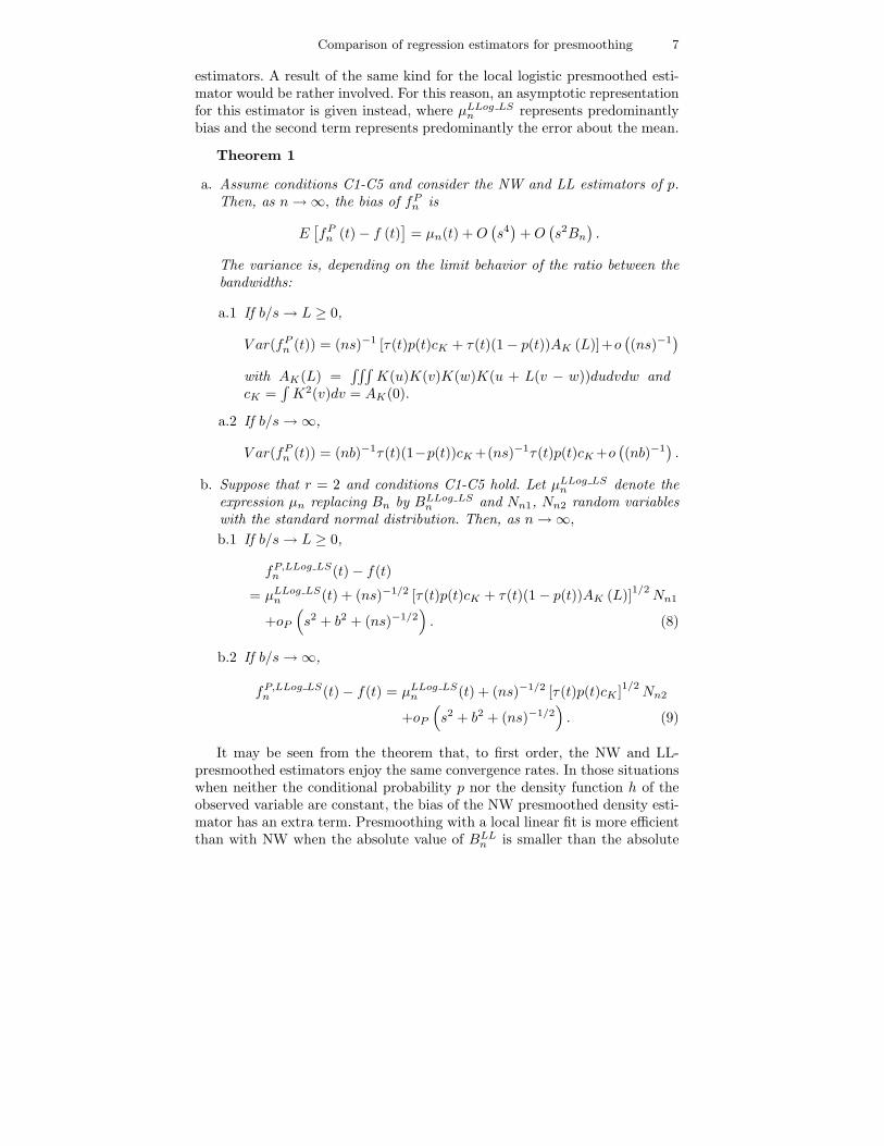
estimators. A result of the same kind for the local logistic presmoothed esti-mator would be rather involved. For this reason, an asymptotic representationfor this estimator is given instead, where µLLog LS

n represents predominantlybias and the second term represents predominantly the error about the mean.

Theorem 1

a. Assume conditions C1-C5 and consider the NW and LL estimators of p.Then, as n→ ∞, the bias of fP

n is

E[fP

n (t) − f (t)]

= µn(t) +O(s4)

+O(s2Bn

).

The variance is, depending on the limit behavior of the ratio between the

bandwidths:

a.1 If b/s→ L ≥ 0,

V ar(fPn (t)) = (ns)−1 [τ(t)p(t)cK + τ(t)(1 − p(t))AK (L)]+o

((ns)−1

)

with AK(L) =∫∫∫

K(u)K(v)K(w)K(u + L(v − w))dudvdw and

cK =∫K2(v)dv = AK(0).

a.2 If b/s→ ∞,

V ar(fPn (t)) = (nb)−1τ(t)(1−p(t))cK +(ns)−1τ(t)p(t)cK +o

((nb)−1

).

b. Suppose that r = 2 and conditions C1-C5 hold. Let µLLog LSn denote the

expression µn replacing Bn by BLLog LSn and Nn1, Nn2 random variables

with the standard normal distribution. Then, as n→ ∞,

b.1 If b/s→ L ≥ 0,

fP,LLog LSn (t) − f(t)

= µLLog LSn (t) + (ns)−1/2 [τ(t)p(t)cK + τ(t)(1 − p(t))AK (L)]

1/2Nn1

+oP

(s2 + b2 + (ns)−1/2

). (8)

b.2 If b/s→ ∞,

fP,LLog LSn (t) − f(t) = µLLog LS

n (t) + (ns)−1/2 [τ(t)p(t)cK ]1/2

Nn2

+oP

(s2 + b2 + (ns)−1/2

). (9)

It may be seen from the theorem that, to first order, the NW and LL-presmoothed estimators enjoy the same convergence rates. In those situationswhen neither the conditional probability p nor the density function h of theobserved variable are constant, the bias of the NW presmoothed density esti-mator has an extra term. Presmoothing with a local linear fit is more efficientthan with NW when the absolute value of BLL

n is smaller than the absolute

8 M.A. Jacome, I. Gijbels and R. Cao

value of BNWn (see the simulations in Section 3). Note that both functions, p

and h, can be easily estimated using the observed data (Z1, δ1), . . . , (Zn, δn).With a nearly uniform design, the derivative of the density function h is

close to zero. In such a case, there is no significant difference, in terms of biasand variance, in presmoothing with the NW estimator or the local linear fit ofp. The same conclusion can be reached when the function p is almost constant,that is, for situations close to the Koziol-Green model (see Koziol and Green(1976)). A similar behavior of the presmoothed density estimator with bothfits of p is expected, but some examples in Section 3 contradict this.

3 Simulation study

A simulation study with four different models has been carried out to illustratethe benefits of the presmoothing mechanism when using the different estima-tors of p. Some of these models have already been used in Cao and Jacome(2004). In Models 1 and 2 the observed variable has been set to a uniform

distribution: Zd= U (0, 1), while for Model 3 and 4 we have Z

d= W (1.75, 5)

and Zd= W (2, 4) respectively, with W (a, b) the Weibull distribution with

scale parameter a, shape parameter b and density function

fW (a,b) (t) = abbtb−1 exp[− (at)

b].

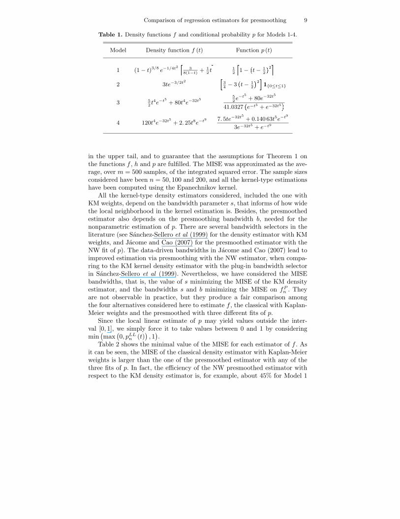
Table 1 gives the density function f to estimate, and the conditional pro-bability p for each model. The four models which we consider are quite diffe-rent in nature. Since the key idea in presmoothing is the nonparametric esti-mation of p, these models have been chosen in order to cover several shapes ofp (almost constant, unimodal, monotone decreasing and with several modes),as it can be seen in Figure 1.

For Models 1 and 2 the design density is uniform, then BNWn (t) = BLL

n (t)for any t ≥ 0. At first glance, one might expect little practical differencebetween both fits in the final presmoothed estimate of the density function.The simulations will show that this is not the case.

To compare the presmoothed estimates with Nadaraya-Watson, local li-near and local logistic fits, as well as the kernel density estimator with Kaplan-Meier weights, we have used the mean integrated squared error (MISE):

MISE(fP

n

)= E

[∫ (fP

n − f)2ω

]=

∫Bias2(fP

n )ω +

∫V ar(fP

n )ω,

with ω (t) = 1{0≤t≤0.9} for Model 1, ω (t) = 1{0≤t≤0.95} for Model 2,ω (t) = 1{0.2≤t≤0.75} for Model 3 and ω (t) = 1{0≤t≤0.75} for Model 4. Thisweighting function has been considered to take positive values just in regionswith observed data and to avoid problems of definition at the right tail. Theseintervals have been chosen in order to discard at most 5% of the distribution

Comparison of regression estimators for presmoothing 9

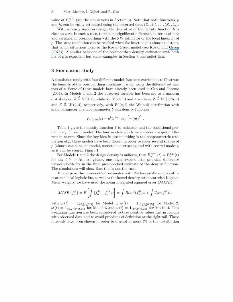
Table 1. Density functions f and conditional probability p for Models 1-4.

Model Density function f (t) Function p (t)

1 (1 − t)3/8e−1/4t2

�3

8(1−t)+ 1

2t

�12

�1 − �t − 1

2 �2�

2 3te−3/2t2�34− 3 �t − 1

2 �2�1{0≤t≤1}

3 52t4e−t5 + 80t4e−32t5

52e−t5 + 80e−32t5

41.0327 �e−t5 + e−32t5�4 120t4e−32t5 + 2. 25t8e−t9 7. 5te−32t5 + 0.140 63t5e−t9

3e−32t5 + e−t9

in the upper tail, and to guarantee that the assumptions for Theorem 1 onthe functions f , h and p are fulfilled. The MISE was approximated as the ave-rage, over m = 500 samples, of the integrated squared error. The sample sizesconsidered have been n = 50, 100 and 200, and all the kernel-type estimationshave been computed using the Epanechnikov kernel.

All the kernel-type density estimators considered, included the one withKM weights, depend on the bandwidth parameter s, that informs of how widethe local neighborhood in the kernel estimation is. Besides, the presmoothedestimator also depends on the presmoothing bandwidth b, needed for thenonparametric estimation of p. There are several bandwidth selectors in theliterature (see Sanchez-Sellero et al (1999) for the density estimator with KMweights, and Jacome and Cao (2007) for the presmoothed estimator with theNW fit of p). The data-driven bandwidths in Jacome and Cao (2007) lead toimproved estimation via presmoothing with the NW estimator, when compa-ring to the KM kernel density estimator with the plug-in bandwidth selectorin Sanchez-Sellero et al (1999). Nevertheless, we have considered the MISEbandwidths, that is, the value of s minimizing the MISE of the KM densityestimator, and the bandwidths s and b minimizing the MISE on fP

n . Theyare not observable in practice, but they produce a fair comparison amongthe four alternatives considered here to estimate f , the classical with Kaplan-Meier weights and the presmoothed with three different fits of p.

Since the local linear estimate of p may yield values outside the inter-val [0, 1], we simply force it to take values between 0 and 1 by consideringmin

(max

(0, pLL

n (t)), 1).

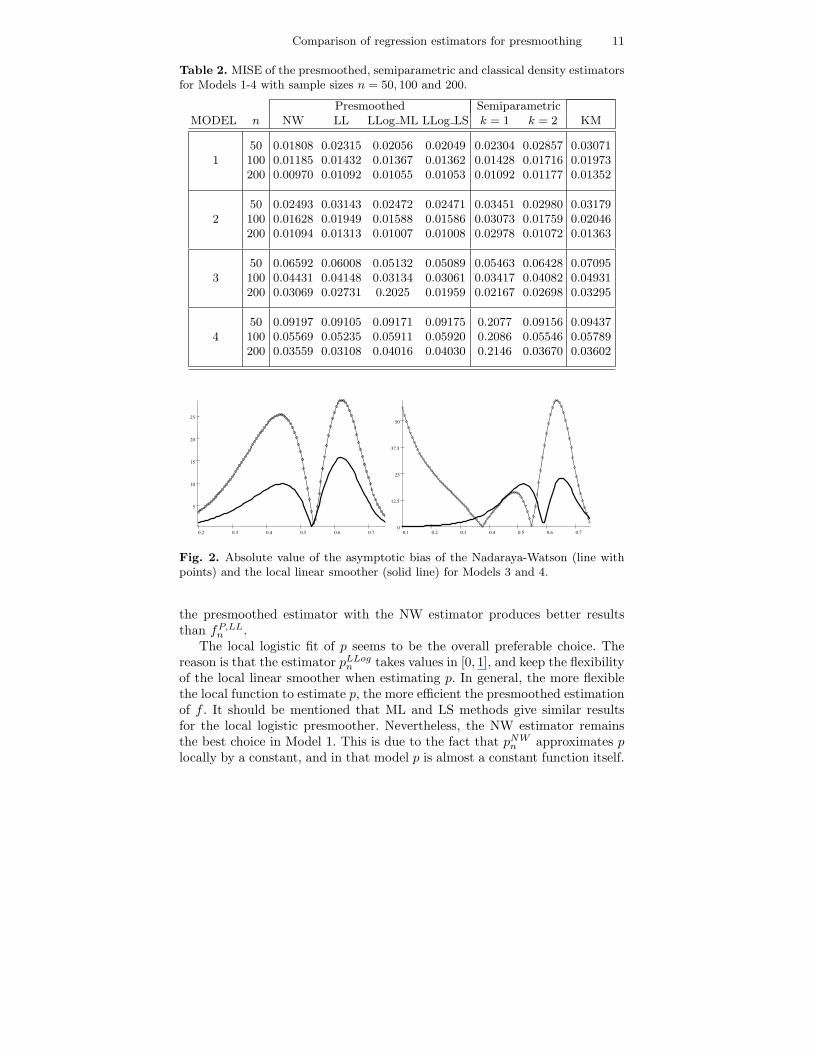
Table 2 shows the minimal value of the MISE for each estimator of f . Asit can be seen, the MISE of the classical density estimator with Kaplan-Meierweights is larger than the one of the presmoothed estimator with any of thethree fits of p. In fact, the efficiency of the NW presmoothed estimator withrespect to the KM density estimator is, for example, about 45% for Model 1

10 M.A. Jacome, I. Gijbels and R. Cao

0.0 0.2 0.4 0.6 0.8 1.0

0.0

0.5

1.0

1.5

2.0

2.5

MODEL 1

f(t)

p(t)

h(t)

0.0 0.5 1.0 1.5 2.0 2.5

0.0

0.2

0.4

0.6

0.8

1.0 f(t)

p(t)

h(t)

MODEL 2

0.0 0.5 1.0 1.5

0

1

2

3

f(t)

p(t)

h(t)

MODEL 3

0.0 0.5 1.0 1.5

0.0

0.5

1.0

1.5

f(t)

p(t)

h(t)

MODEL 4

Fig. 1. Functions p (thick solid line), h (thin solid line) and f (dotted line) forModels 1-4. The vertical lines represent the values a and b for the weight functionω (t) = 1{a≤t≤b}.

and n = 50. Although this efficiency decreases as n → ∞, this means that itis always worth presmoothing regardless the fit of p (see also Cao and Jacome(2004)).

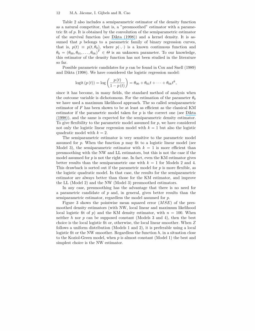
When comparing the NW and local linear fit of p, the performance of thepresmoothed density estimator with a local linear fit, fP,LL

n , is better thanthe one with the Nadaraya-Watson smoother fP,NW

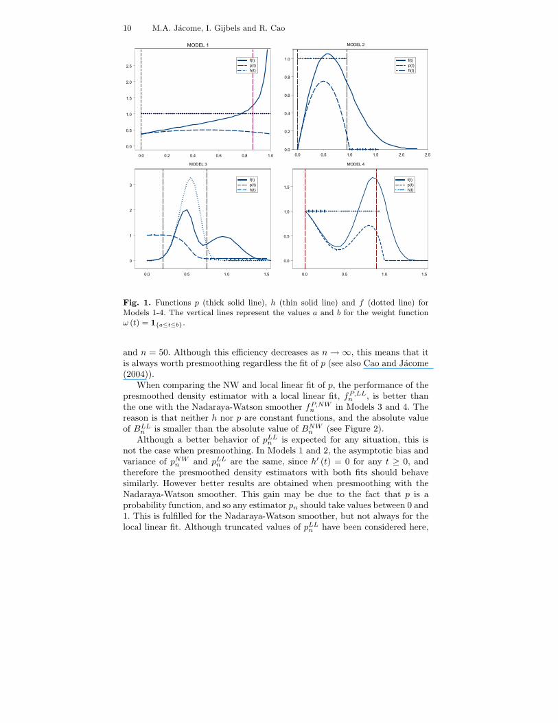
n in Models 3 and 4. Thereason is that neither h nor p are constant functions, and the absolute valueof BLL

n is smaller than the absolute value of BNWn (see Figure 2).

Although a better behavior of pLLn is expected for any situation, this is

not the case when presmoothing. In Models 1 and 2, the asymptotic bias andvariance of pNW

n and pLLn are the same, since h′ (t) = 0 for any t ≥ 0, and

therefore the presmoothed density estimators with both fits should behavesimilarly. However better results are obtained when presmoothing with theNadaraya-Watson smoother. This gain may be due to the fact that p is aprobability function, and so any estimator pn should take values between 0 and1. This is fulfilled for the Nadaraya-Watson smoother, but not always for thelocal linear fit. Although truncated values of pLL

n have been considered here,

Comparison of regression estimators for presmoothing 11

Table 2. MISE of the presmoothed, semiparametric and classical density estimatorsfor Models 1-4 with sample sizes n = 50, 100 and 200.

Presmoothed SemiparametricMODEL n NW LL LLog ML LLog LS k = 1 k = 2 KM

150100200

0.018080.011850.00970

0.023150.014320.01092

0.020560.013670.01055

0.020490.013620.01053

0.023040.014280.01092

0.028570.017160.01177

0.030710.019730.01352

250100200

0.024930.016280.01094

0.031430.019490.01313

0.024720.015880.01007

0.024710.015860.01008

0.034510.030730.02978

0.029800.017590.01072

0.031790.020460.01363

350100200

0.065920.044310.03069

0.060080.041480.02731

0.051320.031340.2025

0.050890.030610.01959

0.054630.034170.02167

0.064280.040820.02698

0.070950.049310.03295

450100200

0.091970.055690.03559

0.091050.052350.03108

0.091710.059110.04016

0.091750.059200.04030

0.20770.20860.2146

0.091560.055460.03670

0.094370.057890.03602

0.70.60.50.40.30.2

25

20

15

10

5

0.70.60.50.40.30.20.1

50

37.5

25

12.5

0

Fig. 2. Absolute value of the asymptotic bias of the Nadaraya-Watson (line withpoints) and the local linear smoother (solid line) for Models 3 and 4.

the presmoothed estimator with the NW estimator produces better resultsthan fP,LL

n .The local logistic fit of p seems to be the overall preferable choice. The

reason is that the estimator pLLogn takes values in [0, 1], and keep the flexibility

of the local linear smoother when estimating p. In general, the more flexiblethe local function to estimate p, the more efficient the presmoothed estimationof f . It should be mentioned that ML and LS methods give similar resultsfor the local logistic presmoother. Nevertheless, the NW estimator remainsthe best choice in Model 1. This is due to the fact that pNW

n approximates plocally by a constant, and in that model p is almost a constant function itself.

12 M.A. Jacome, I. Gijbels and R. Cao

Table 2 also includes a semiparametric estimator of the density functionas a natural competitor, that is, a ”presmoothed” estimator with a parame-tric fit of p. It is obtained by the convolution of the semiparametric estimatorof the survival function (see Dikta (1998)) and a kernel density. It is as-sumed that p belongs to a parametric family of binary regression curves,that is, p(t) ≡ p(t, θ0), where p(·, ·) is a known continuous function and

θ0 = (θ00, θ01, . . . , θ0k)T

∈ Θ is an unknown parameter. To our knowledge,this estimator of the density function has not been studied in the literatureso far.

Possible parametric candidates for p can be found in Cox and Snell (1989)and Dikta (1998). We have considered the logistic regression model:

logit (p (t)) = log

(p (t)

1 − p (t)

)= θ00 + θ01t+ · · · + θ0kt

k,

since it has become, in many fields, the standard method of analysis whenthe outcome variable is dichotomous. For the estimation of the parameter θ0we have used a maximum likelihood approach. The so called semiparametricestimator of F has been shown to be at least as efficient as the classical KMestimator if the parametric model taken for p is the correct one (see Dikta(1998)), and the same is expected for the semiparametric density estimator.To give flexibility to the parametric model assumed for p, we have considerednot only the logistic linear regression model with k = 1 but also the logisticquadratic model with k = 2.

The semiparametric estimator is very sensitive to the parametric modelassumed for p. When the function p may fit to a logistic linear model (seeModel 3), the semiparametric estimator with k = 1 is more efficient thanpresmoothing with the NW and LL estimators, but this is not the case if themodel assumed for p is not the right one. In fact, even the KM estimator givesbetter results than the semiparametric one with k = 1 for Models 2 and 4.This drawback is sorted out if the parametric model for p is more flexible, asthe logistic quadratic model. In that case, the results for the semiparametricestimator are always better than those for the KM estimator, and improvethe LL (Model 2) and the NW (Model 3) presmoothed estimators.

In any case, presmoothing has the advantage that there is no need fora parametric candidate of p and, in general, gives better results than thesemiparametric estimator, regardless the model assumed for p.

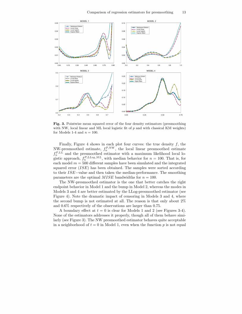
Figure 3 shows the pointwise mean squared error (MSE) of the pres-moothed density estimators (with NW, local linear and maximum likelihoodlocal logistic fit of p) and the KM density estimator, with n = 100. Whenneither h nor p can be supposed constant (Models 3 and 4), then the bestchoice is the local logistic fit or, otherwise, the local linear smoother. When Zfollows a uniform distribution (Models 1 and 2), it is preferable using a locallogistic fit or the NW smoother. Regardless the function h, in a situation closeto the Koziol-Green model, when p is almost constant (Model 1) the best andsimplest choice is the NW estimator.

Comparison of regression estimators for presmoothing 13

0.00 0.15 0.30 0.45 0.60 0.75 0.90

0.00

0.01

0.02

0.03

0.04

0.05MODEL 1

Nadaraya-Watson

Local linear

Local logistic

Kaplan-Meier

0.0 0.2 0.4 0.6 0.8 1.0

0.00

0.02

0.04

0.06

0.08

0.10MODEL 2

Nadaraya-Watson

Local linear

Local logistic

Kaplan-Meier

0.2 0.3 0.4 0.5 0.6 0.7

0.0

0.1

0.2

0.3MODEL 3

Nadaraya-Watson

Local linear

Local logistic

Kaplan-Meier

0.00 0.25 0.50 0.75

0.00

0.05

0.10

0.15

0.20

0.25

MODEL 4

Nadaraya-Watson

Local linear

Local logistic

Kaplan-Meier

Fig. 3. Pointwise mean squared error of the four density estimators (presmoothingwith NW, local linear and ML local logistic fit of p and with classical KM weights)for Models 1-4 and n = 100.

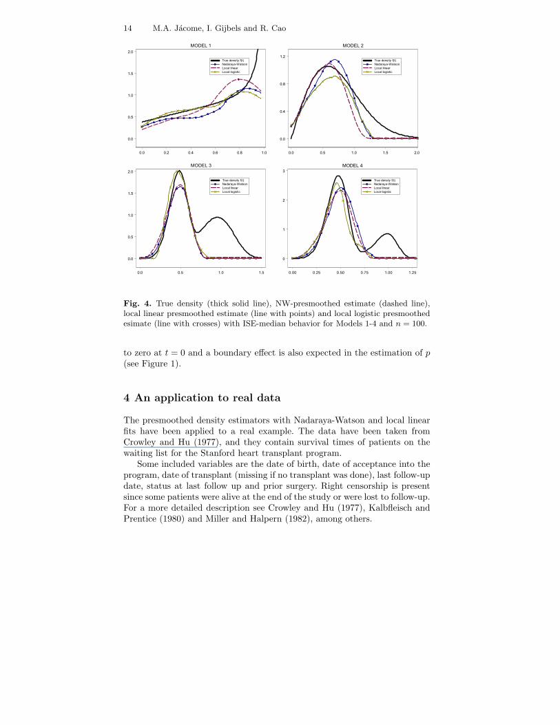
Finally, Figure 4 shows in each plot four curves: the true density f , theNW-presmoothed estimate, fP,NW

n , the local linear presmoothed estimatefP,LL

n and the presmoothed estimator with a maximum likelihood local lo-gistic approach, fP,LLog ML

n , with median behavior for n = 100. That is, foreach model m = 500 different samples have been simulated and the integratedsquared error (ISE) has been obtained. The samples were sorted accordingto their ISE−value and then taken the median-performance. The smoothingparameters are the optimal MISE bandwidths for n = 100.

The NW-presmoothed estimator is the one that better catches the rightendpoint behavior in Model 1 and the bump in Model 2, whereas the modes inModels 3 and 4 are better estimated by the LLog-presmoothed estimator (seeFigure 4). Note the dramatic impact of censoring in Models 3 and 4, wherethe second bump is not estimated at all. The reason is that only about 2%and 0.6% respectively of the observations are larger than 0.75.

A boundary effect at t = 0 is clear for Models 1 and 2 (see Figures 3-4).None of the estimators addresses it properly, though all of them behave simi-larly (see Figure 3). The NW presmoothed estimator behaves quite acceptablein a neighborhood of t = 0 in Model 1, even when the function p is not equal

14 M.A. Jacome, I. Gijbels and R. Cao

0.0 0.2 0.4 0.6 0.8 1.0

0.0

0.5

1.0

1.5

2.0

MODEL 1

True density f(t)

Nadaraya-Watson

Local linear

Local logistic

0.0 0.5 1.0 1.5 2.0

0.0

0.4

0.8

1.2

MODEL 2

True density f(t)

Nadaraya-Watson

Local linear

Local logistic

0.0 0.5 1.0 1.5

0.0

0.5

1.0

1.5

2.0

MODEL 3

True density f(t)

Nadaraya-Watson

Local linear

Local logistic

0.00 0.25 0.50 0.75 1.00 1.25

0

1

2

3

MODEL 4

True density f(t)

Nadaraya-Watson

Local linear

Local logistic

Fig. 4. True density (thick solid line), NW-presmoothed estimate (dashed line),local linear presmoothed estimate (line with points) and local logistic presmoothedesimate (line with crosses) with ISE-median behavior for Models 1-4 and n = 100.

to zero at t = 0 and a boundary effect is also expected in the estimation of p(see Figure 1).

4 An application to real data

The presmoothed density estimators with Nadaraya-Watson and local linearfits have been applied to a real example. The data have been taken fromCrowley and Hu (1977), and they contain survival times of patients on thewaiting list for the Stanford heart transplant program.

Some included variables are the date of birth, date of acceptance into theprogram, date of transplant (missing if no transplant was done), last follow-update, status at last follow up and prior surgery. Right censorship is presentsince some patients were alive at the end of the study or were lost to follow-up.For a more detailed description see Crowley and Hu (1977), Kalbfleisch andPrentice (1980) and Miller and Halpern (1982), among others.

Comparison of regression estimators for presmoothing 15

1 3 10 25 75 150 400 1500 5000

Survival time (in days)

0.00

0.01

0.02

0.03

Ab

so

lute

va

lue

of th

e e

stim

ate

d a

sym

pto

tic b

ias B

n

Nadaraya-Watson

Local linear

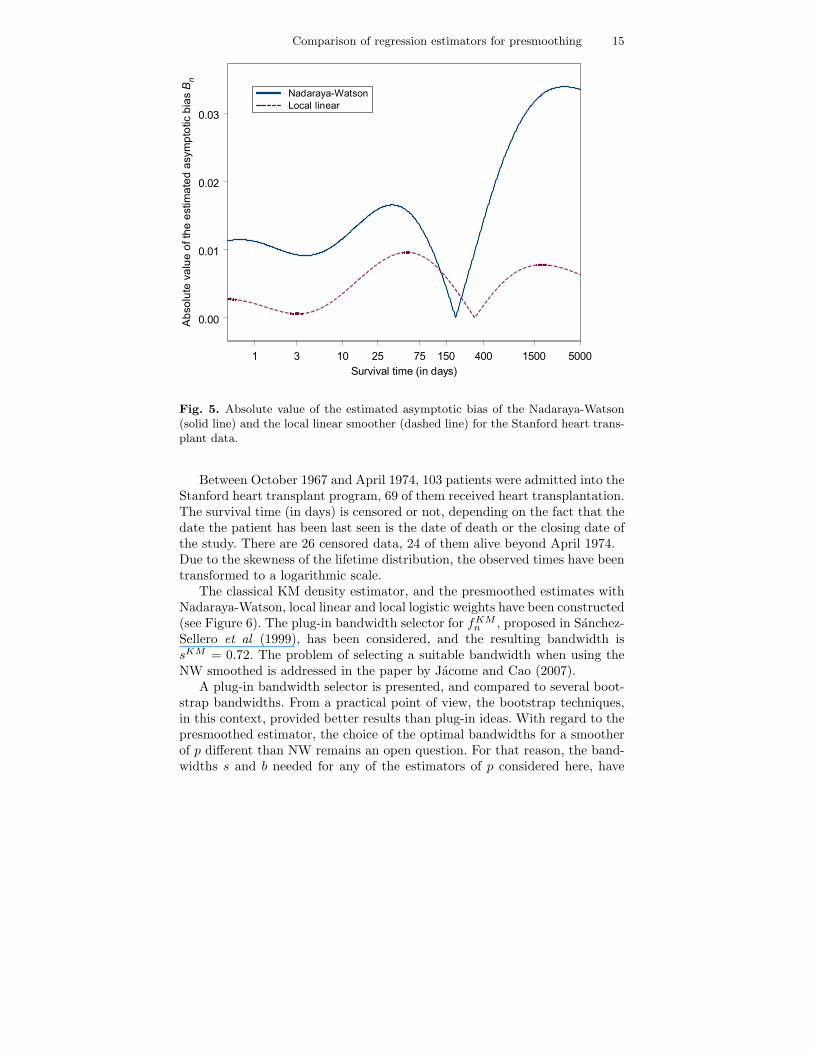
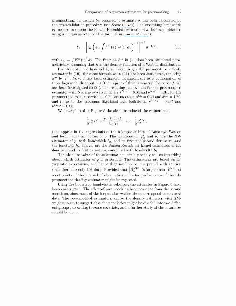
Fig. 5. Absolute value of the estimated asymptotic bias of the Nadaraya-Watson(solid line) and the local linear smoother (dashed line) for the Stanford heart trans-plant data.

Between October 1967 and April 1974, 103 patients were admitted into theStanford heart transplant program, 69 of them received heart transplantation.The survival time (in days) is censored or not, depending on the fact that thedate the patient has been last seen is the date of death or the closing date ofthe study. There are 26 censored data, 24 of them alive beyond April 1974.Due to the skewness of the lifetime distribution, the observed times have beentransformed to a logarithmic scale.

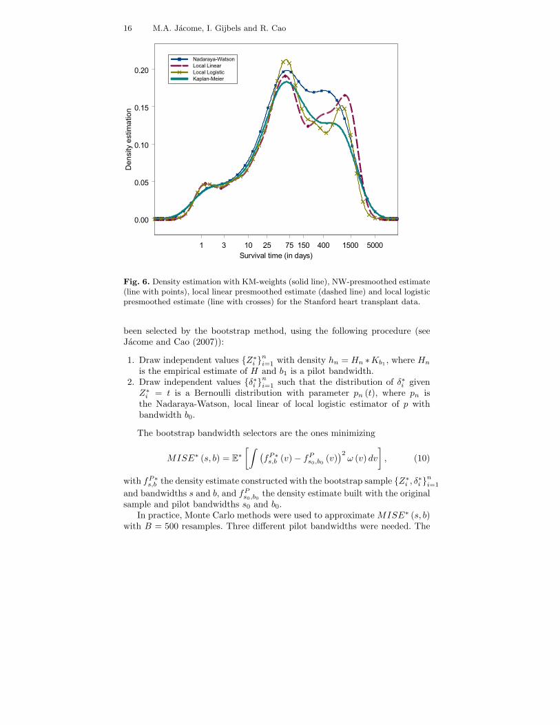
The classical KM density estimator, and the presmoothed estimates withNadaraya-Watson, local linear and local logistic weights have been constructed(see Figure 6). The plug-in bandwidth selector for fKM

n , proposed in Sanchez-Sellero et al (1999), has been considered, and the resulting bandwidth issKM = 0.72. The problem of selecting a suitable bandwidth when using theNW smoothed is addressed in the paper by Jacome and Cao (2007).

A plug-in bandwidth selector is presented, and compared to several boot-strap bandwidths. From a practical point of view, the bootstrap techniques,in this context, provided better results than plug-in ideas. With regard to thepresmoothed estimator, the choice of the optimal bandwidths for a smootherof p different than NW remains an open question. For that reason, the band-widths s and b needed for any of the estimators of p considered here, have

16 M.A. Jacome, I. Gijbels and R. Cao

1 3 10 25 75 150 50001500400

Survival time (in days)

0.00

0.05

0.10

0.15

0.20

De

nsity e

stim

atio

n

Nadaraya-Watson

Local Linear

Local Logistic

Kaplan-Meier

Fig. 6. Density estimation with KM-weights (solid line), NW-presmoothed estimate(line with points), local linear presmoothed estimate (dashed line) and local logisticpresmoothed estimate (line with crosses) for the Stanford heart transplant data.

been selected by the bootstrap method, using the following procedure (seeJacome and Cao (2007)):

1. Draw independent values {Z∗i }

ni=1 with density hn = Hn ∗Kb1 , where Hn

is the empirical estimate of H and b1 is a pilot bandwidth.2. Draw independent values {δ∗i }

ni=1 such that the distribution of δ∗i given

Z∗i = t is a Bernoulli distribution with parameter pn (t), where pn is

the Nadaraya-Watson, local linear of local logistic estimator of p withbandwidth b0.

The bootstrap bandwidth selectors are the ones minimizing

MISE∗ (s, b) = E∗

[∫ (fP∗

s,b (v) − fPs0,b0 (v)

)2ω (v) dv

], (10)

with fP∗s,b the density estimate constructed with the bootstrap sample {Z∗

i , δ∗i }

ni=1

and bandwidths s and b, and fPs0,b0

the density estimate built with the originalsample and pilot bandwidths s0 and b0.

In practice, Monte Carlo methods were used to approximate MISE∗ (s, b)with B = 500 resamples. Three different pilot bandwidths were needed. The

Comparison of regression estimators for presmoothing 17

presmoothing bandwidth b0, required to estimate p, has been calculated bythe cross-validation procedure (see Stone (1975)). The smoothing bandwidthb1, needed to obtain the Parzen-Rosenblatt estimate of h, has been obtainedusing a plug-in selector for the formula in Cao et al (1994):

b1 =

[iK

(dK

∫h′′′ (v)

2ω (v) dv

)−1]1/7

n−1/7, (11)

with iK =∫K ′′ (v)

2dv. The function h′′′ in (11) has been estimated para-

metrically, assuming that h is the density function of a Weibull distribution.For the last pilot bandwidth, s0, used to get the presmoothed density

estimator in (10), the same formula as in (11) has been considered, replacingh′′′ by f ′′′. Now, f has been estimated parametrically as a combination ofthree lognormal distributions (the impact of this parametric choice for f hasnot been investigated so far). The resulting bandwidths for the presmoothedestimator with Nadaraya-Watson fit are sNW = 0.64 and bNW = 1.31, for thepresmoothed estimator with local linear smoother, sLL = 0.41 and bLL = 4.70,and those for the maximum likelihood local logistic fit, sLLog = 0.435 andbLLog = 0.05.

We have plotted in Figure 5 the absolute value of the estimations:

1

2p′′n (t) +

p′n (t)h′n (t)

hn (t)and

1

2p′′n(t),

that appear in the expressions of the asymptotic bias of Nadaraya-Watsonand local linear estimators of p. The functions pn, p′n and p′′n are the NWestimator of p, with bandwidth b0, and its first and second derivative, andthe functions hn and h′n are the Parzen-Rosenblatt kernel estimators of thedensity h and its first derivative, computed with bandwidth b1.

The absolute value of these estimations could possibly tell us somethingabout which estimator of p is preferable. The estimations are based on as-ymptotic expressions, and hence they need to be interpreted with caution

since there are only 103 data. Provided that∣∣∣BNW

n

∣∣∣ is larger than∣∣∣BLL

n

∣∣∣ at

most points of the interval of observation, a better performance of the LL-presmoothed density estimator might be expected.

Using the bootstrap bandwidths selectors, the estimates in Figure 6 havebeen constructed. The effect of presmoothing becomes clear from the secondmonth on, since most of the largest observation times correspond to censoreddata. The presmoothed estimators, unlike the density estimator with KM-weights, seem to suggest that the population might be divided into two differ-ent groups, according to some covariate, and a further study of the covariatesshould be done.

18 M.A. Jacome, I. Gijbels and R. Cao

5 Conclusions

Local polynomial estimators of the regression function, and particularly thelocal linear estimator, have great appealing properties with respect to theNadaraya-Watson smoother. This one has bias problems, especially at theregion where the derivative of the design density is large. Local polynomialsmoothing attends to the bias problem while keeps asymptotically the samevariance.

When estimating the regression function p in the presmoothing procedure,the preference for the local linear fit rather than the NW smoother is not soclear. The key lies in the function p to be estimated, and in h, the densityfunction of the observed variable Z. Both functions can be easily estimatedusing the sample (Zi, δi), for i = 1, . . . , n.

The local linear estimator remains being the best choice at the pointswhere both the functions h and p are not constant, more specifically, wherethe bias of the NW-presmoothed density estimator is larger than the one withlocal linear estimates.

However, in the cases when either h or p can be supposed to be almost con-stant, the NW estimator is clearly preferable. The gain of the NW estimatoris especially remarkable if the function p is almost constant.

In any case, regardless of the shape of p and h, the local logistic fit is acompetitive method that may outperform the other estimators of p consideredin this paper.

6 Appendix

Proof. of Theorem 1. Consider the relation between fPn and the presmoothed

distribution estimator FPn :

fPn (t) =

∫Ks (t− v) dFP

n (v)

and, under assumptions C1-C4, the iid representation of FPn in Jacome and

Cao (2006):

FPn (t) = F (t) +

1

n

n∑

i=1

εi (t) + γ (t) +Rn (t)

with

εi(t) = (1 − F (t))

[1{Zi≤t} −H(t)

1 −H(t)p(t) −

∫ t

0

1{Zi≤v} −H(v)

1 −H(v)p′(v)dv

],

γ(t) = (1 − F (t))

∫ t

0

h(v)

1 −H(v)[pn(v) − p(v)] dv,

with pn an estimator of p, and

Comparison of regression estimators for presmoothing 19

supt∈[0,tH ]

|Rn(t)| = O

((b2 + (nb)−1(lnn)1/2

)2

(lnn)2).

For the NW and LL estimator of p, one may infer the following representationof fP

n :

fPn (t) =

∫Ks (t− v) dF (t) +A (t) −B (t) + C (t)

+

∫Ks (t− v)

[(1 − F (v))

∫ v

0

h(w)

1 −H(w)(E [pn(w)] − p(w))

]′dv + en(t),

where

A (t) =1

n

n∑

i=1

∫Ks (t− v) dεi (v) , (12)

B (t) =

∫Ks (t− v) f (v)

∫ v

0

h(w)

1 −H(w)(pn(w) − E [pn(w)]) dwdv,

C (t) =

∫Ks (t− v)

1 − F (v)

1 −H(v)h(v) (pn(v) − E [pn(v)]) dv,

and

supt∈[0,tH ]

|en(t)| = O

(s−1

(b2 + (nb)−1(lnn)1/2

)2

(lnn)2).

In view of assumption C1, the dominant terms in the bias and variance of thepresmoothed estimator fP

n are the same as those of the iid representation. SeeTheorem 2.2 in Jacome and Cao (2007) for details with the NW estimator.

Since E[A(t)] = E[B(t)] = E[C(t)] = 0, and under condition C5, then itis easy to show that the bias of the presmoothed density estimator is

E[fP

n (t)]− f (t)

=

∫Ks (t− v) f (t) − f (t) +

∫Ks (t− v)

[(1 − F (v))

∫ v

0

h(w)Bn(w)

1 −H(w)dw

]′dv

=1

2dKf

′′ (t) s2 +

[(1 − F (t))

∫ t

0

h(v)Bn(v)

1 −H(v)dv

]′+O

(s4)

+O(s2Bn

).

On the other hand, the variance of fPn is

V ar(fP

n

)= V ar (A) + V ar (B) + V ar (C)

−2Cov (A,B) + 2Cov (A,C) − 2Cov (B,C) . (13)

Straightforward, although long and tedious calculations give that the domi-nant terms in the V ar(fP

n ) are

V ar (A) =1

ns

(1 − F (t)

1 −H (t)

)2

p2 (t)h (t) cK +O

(1

n

), (14)

20 M.A. Jacome, I. Gijbels and R. Cao

that does not depend on the estimator pn. For B and C, we have

V ar (B) =

∫∫Ks (t− v1)Ks (t− v2) f (v1) f (v2)

×

∫ v1

0

∫ v2

0

h(w1)

1 −H(w1)

h(w2)

1 −H(w2)

×E [(pn(w1) − E [pn(w1)]) (pn(w2) − E [pn(w2)])] dw1dw2dv1dv2,

V ar (C) =

∫∫Ks (t− v1)Ks (t− v2)

1 − F (v1)

1 −H(v1)

1 − F (v2)

1 −H(v2)h(v1)h(v2)

×E [(pn(v1) − E [pn(v1)]) (pn(v2) − E [pn(v2)])] dv1dv2,

and

Cov (B,C) =

∫∫Ks (t− v1)Ks (t− v2) f (v1)

1 − F (v2)

1 −H(v2)h(v2)

∫ v1

0

h(w)

1 −H(w)

×E [(pn(w) − E [pn(w)]) (pn(v2) − E [pn(v2)])] dwdv1dv2.

Next, we need to compute the expectations

E [(pn(x) − E [pn(x)]) (pn(y) − E [pn(y)])] (15)

for the NW and LL estimators of p. We are going to show that both estimatorssatisfy

E [(pn(x) − E [pn(x)]) (pn(y) − E [pn(y)])]

=1

h (x)h (y)

1

nE [Kb (Z − x)Kb (Z − y) p(Z) (1 − p (Z))] (1 + o(1)). (16)

In this case, we have

V ar (B) = O

(1

n

)and Cov(B,C) = O

(1

n

)(17)

and, depending on the ratio b/s between the bandwidths,

V ar (C) =1

ns

(1 − F (t)

1 −H (t)

)2

p (t) (1 − p (t))h (t)AK (L) + o

(1

ns

)(18)

if b/s→ L ≥ 0, and

V ar (C) =1

nb

(1 − F (t)

1 −H (t)

)2

p (t) (1 − p (t))h (t) cK + o

(1

nb

)(19)

if b/s→ ∞.Consequently, combination of (13), (14), (17), (18) and (19) gives the

asymptotic variance of the presmoothed estimator fPn with the NW and LL

estimators. The final step is to prove (16) for both estimators of p.

Comparison of regression estimators for presmoothing 21

The NW estimator can be decomposed as follows:

pNWn (t) =

ψn (t)

h (t)−p (t)

h (t)(hn (t) − h (t))−

1

h (t)

(pNW

n (t) − p (t))(hn (t) − h (t))

where

ψn (t) =1

n

n∑

i=1

Kb (Zi − t) δi and hn (t) =1

n

n∑

i=1

Kb (Zi − t) .

Therefore, by a standard argument,

E[pNW

n (t)]

=1

h (t)E [Kb (Z − t) p (Z)] +O

(b2).

So, the dominant term in the expectation (15) is

1

h (x)h (y)

1

nE [Kb (Z − x)Kb (Z − y) p(Z) (1 − p (Z))] .

As for the local linear estimator, let Wn(x) =∑n

i=1 wi,n(x)/(n2b4) andW (x) = dKh

2(x). Using that 1/Wn(x) = 1/W (x) + o4(1), (see (6.6) in Fan(1993)), that is,

n2b4

n∑i=1

ωi,n (x)=

1

dKh2 (x)+ rn (x) with sup

hZ,δ∈C2

E∣∣r4n (x)

∣∣ = o (1) ,

where hZ,δ(·, ·) is the joint ”density” of (Z, δ),

C2 = {hZ,δ(·, ·) : |p(x) − p(x0) − p′(x0)(x− x0)| ≤ C(x− x0)

2

2, |p(x0)| ≤ C∗}

∩{hZ,δ(·, ·) : σ2(x) ≤ B, h(x0) ≥ b, |h(x) − h(y)| ≤ c|x− y|α}

and C,C∗, B, b, c and α are positive constants.Then the expectation in (15) is

E

n∑i=1

(Yi − E

[pLL

n (x)])ωi,n (x)

n∑i=1

ωi,n (x)

n∑j=1

(Yj − E

[pLL

n (y)])ωj,n (y)

n∑j=1

ωj,n (y)

+ o

(1

(nb)4

)

=1

n4b81

d2Kh

2 (x)h2 (y)

×E

n∑

i=1

(Yi − p (x))ωi,n (x)n∑

j=1

(Yj − p (y))ωj,n (y)

(1 + o (1)) . (20)

22 M.A. Jacome, I. Gijbels and R. Cao

Next, introducing p (Zi) in each sum, we have

E

n∑

i=1

(Yi − p (x))ωi,n (x) ×n∑

j=1

(Yj − p (y))ωj,n (y)

= nE[(Y − p (Z))

2ωn (x)ωn (y)

]

+nE [(p (Z) − p (x)) (p (Z) − p (y))ωn (x)ωn (y)]

+n (n− 1)E [(p (Z) − p (x))ωn (x)] × E [(p (Z) − p (y))ωn (y)] .

To handle the previous terms, recall ωn(t) = Kb(Z−t) (Sn,2(t) − (Z − t)Sn,1(t))and

Sn,j(t) =n∑

i=1

Kb(Zi − t)(Zi − t)j .

Standard Taylor expansions and symmetry of the kernel K yield the followingresults, for ξ any function of the variable Z:

E [ξ (Z)ωn (x)] = (n− 1) b3dK

{h (x)E

[K

(x− Z

b

)ξ (Z)

]

−h′ (x)E

[K

(x− Z

b

)ξ (Z) (x− Z)

]} (1 +O

(b2))

and

E [ξ (Z)ωn (x)ωn (y)]

= n2b6d2Kh (x)h (y)E

[ξ (Z)K

(x− Z

b

)K

(y − Z

b

)] (1 +O

(b2)).

Then, conditioning on covariates Zi, i = 1, . . . , n

E

n∑

i=1

(Yi − p (x))ωi,n (x) ×n∑

j=1

(Yj − p (y))ωj,n (y)

= n3b6d2Kh (x)h (y)E

[σ (Z)K

(x− Z

b

)K

(y − Z

b

)](1 + o (1)) .

This together with (20) entail (16).With respect to the local logistic estimator of p, we follow the lines of the

proof of Theorem 1 in Hall et al (1999). Note that pLLog LSn (t) = g(0, α(t)),

with α the minimizer of

Rn(α, t) =n∑

i=1

Kb (t− Zi) [δi − g(Zi − t, α)]2 (21)

and put p∗n(t) = g(0, α∗(t)), with α∗ the minimizer of

Comparison of regression estimators for presmoothing 23

R∗n (α, t) =

n∑

i=1

Kb (Zi − t)

×

δi −r−1∑

j=0

1

j!g(j) (0, α) (Zi − t)

j−

1

r!g(r) (ci (Zi − t) , α) (Zi − t)

r

2

with ci ∈ [0, 1]. By Taylor expansion of g in (21), R∗n(α, t) is defined as Rn(α, t)

with α in g(r) (ci (Zi − t) , α) replaced by α. To prove the theorem for thepresmoothed estimator with pLLog LS

n , it suffices to derive (8) and (9) for

fP∗n (t) =

∫Ks (t− v) dF (t) +A(t) +B∗(t)

with A in (12) and

B∗(t) =

∫Ks (t− v) d

[(1 − F (v))

∫ v

0

h(u)

1 −H(u)[p∗n(u) − p(u)] du

], (22)

and also to prove that

fP,LLogn (t) = fP∗

n (t) + oP (br) . (23)

To show that (8) and (9) hold for fP∗n , let Sn (t) be the r× r matrix with

si+j−2 (t) as its (i, j)th element, with

sj (t) =(nbj)−1 n∑

i=1

Kb (Zi − t) (Zi − t)j.

DefineWnb (u, t) = (1, 0, ..., 0)S−1

n (t)(1, u, ..., ur−1

)TK (u)

and Wnb (u, t) = Wn

(ub , t), and put

Ri (t) =1

r!

[p(r) (t+ c′i (Zt − t)) − g(r) (ci (Zi − t) , α)

]with ci, c

′i ∈ [0, 1] .

In this notation we have, by the definition of p∗n,

B∗ (t) = (nb)−1

n∑

i=1

∫Ks (t− v) d

{(1 − F (v))

∫ v

0

h(u)

1 −H(u)

× [Wnb (Zi − u, u) (δi − p (Zi) +Ri (u) (Zi − u)r)] du} . (24)

Define κi =∫uiK (u) du. By the ergodic theorem, Sn (t) → h (t)S (t) in

probability, where S (t) denotes the r×r matrix with κi+j−2 in position (i, j).

Let κ(i,j) be the (i, j)th element of S−1, and put ξi (t) =

r∑j=1

κ(1,j)(

Zi−tb

)j−1.

Noting the representation (24), we may prove that

24 M.A. Jacome, I. Gijbels and R. Cao

fP∗n (t) − f (t)∫

Ks (t− v) dF (t) +A (t) +B∗1 (t) +B∗

2 (t) − f(t)

P→ 1, (25)

with

B∗1 (t) =

1

n

n∑

i=1

∫Ks (t− v) d

{(1 − F (v))

∫ v

0

h(u)

1 −H(u)

×[h−1 (u) ξi (u)Kb (Zi − u) (δi − p (Zi))

]du},

B∗2 (t) =

1

n

n∑

i=1

∫Ks (t− v) d

{(1 − F (v))

∫ v

0

h(u)

1 −H(u)

×[h−1 (u) ξi (u)Kb (Zi − u)Ri (u) (Zi − u)

r]du}.

To prove (25) it is sufficient to show that

B∗(t) = B∗1(t) +B∗

2(t) + oP (B∗(t)) . (26)

Following Hall et al (1999),

p∗n (u) − p (u)

1n

n∑i=1

[h−1 (u) ξi (u)Kb (Zi − u) (δi − p (Zi) +Ri (u) (Zi − u)r)]

P→ 1 (R1)

which implies

p∗n (u) − p (u) =1

n

n∑

i=1

[ξi (u)

h (u)Kb (Zi − u) (δi − p (Zi) +Ri (u) (Zi − u)

r)

]

+oP (p∗n (u) − p (u)). (27)

Since maxu |p∗n(u) − p(u)| ≤ 1, then using (27) in expression (22) gives (26).The first summand in the denominator of (25) is a deterministic term

∫Ks (t− v) dF (t) = f (t) +

1

2dKf

′′ (t) s2 + o(s2).

As for B∗2 in (25), by the ergodic theorem,

B∗2 (t) =

∫Ks (t− v) d

{(1 − F (v))

∫ v

0

h(u)

1 −H(u)BLLog LS

n (u) du

}+ oP (br)

with BLLog LSn given in (7).

The remaining terms in the denominator of (25) are

A (t) +B∗1 (t) =

1

n

n∑

i=1

∫Ks (t− v) dωb (Zi, δi, v)

Comparison of regression estimators for presmoothing 25

where

ωb (Zi, δi, v) = εi (v) + (1 − F (v))

∫ v

0

h(u)

1 −H(u)

×[h−1 (u) ξi (u)Kb (Zi − u) (δi − p (Zi))

]du.

Conditioning on Zi, we have E[∫Ks (t− v) dωb (Zi, δi, v)

]= 0. Then, by

the CLT, it follows that (ns)−1/2

(A (t) +B∗1 (t)) is asymptotically normal

with mean 0 and variance

sE

[(∫Ks (t− v) dωb (Z1, δ1, v)

)2]

= sE

[(∫Ks (t− v) dε1 (v)

)2]

+ sE

[(∫Ks (t− v) d

((1 − F (v))

∫ v

0

ξ1 (u)

1 −H(u)Kb (Z1 − u) (δ1 − p (Z1)) du

))2]

+ 2sE

[∫Ks (t− v) dε1 (v)

∫Ks (t− w)

×d

((1 − F (w))

∫ w

0

ξ1 (u)

1 −H(u)Kb (Z1 − u) (δ1 − p (Z1)) du

)]. (28)

By simple Taylor expansions and the symmetry of the kernel, the firstterm in (28) converges to

(1 − F (t)

1 −H (t)

)2

p2 (t)h (t) cK .

As for the remaining terms in (28), note that for the local linear logisticestimator r = 2 and ξ (t) = 1. Then, if b/s → L ≥ 0, the second termconverges to (

1 − F (t)

1 −H (t)

)2

p (t) (1 − p (t))h (t)AK (L) ,

and the last one is asymptotically negligible. In the case when b/s→ ∞, thenit is easy to see that the dominant term of the second summand in (28) is

s

b

(1 − F (t)

1 −H (t)

)2

p (t) (1 − p (t))h (t) cK

that converges to zero. Combining the results in this paragraph, we obtainthe version of (8) and (9) for fP∗

n instead of fP,LLogn .

The final step is to prove (23), that is,

∫Ks (t− v) d

[(1 − F (v))

∫ v

0

h(u)

1 −H(u)b−r

[pLLog

n (u) − p∗n(u)]du

]P→ 0.

26 M.A. Jacome, I. Gijbels and R. Cao

This convergence follows from the result (A.1) in Hall et al (1999):

pLLogn (t) − p∗n(t) = oP (br).

This completes the proof.

7 Acknowledgments

We thank the referees for their very helpful comments which led to a consider-able improvement of the paper. Research supported in part by MCyT GrantMTM2005-00429 (ERDF support included) and by XUGA Grant PGIDT03-PXIC10505PN for first and third authors. The second author gratefully ac-knowledges the Research Fund K. U. Leuven (GOA/2007/4) for financial sup-port.

Part of this research was carried out during a visit of the first author to theInstitute de Statistique, Universite Catholique de Louvain (Louvain-la-Neuve,Belgium).

References

1. Cao, R., Cuevas, A. and Gonzalez-Manteiga, W. (1994) A comparative study ofseveral smoothing methods in density estimation, Comput. Statist. Data Anal.,17, 153–176.

2. Cao, R., Lopez-de-Ullibarri, I., Janssen, P. and Veraverbeke, N. (2005) Pres-moothed Kaplan-Meier and Nelson-Aalen estimators, J. Nonparametr. Stat.,

17, 31–56.3. Cao, R. and Jacome, M.A. (2004) Presmoothed kernel density estimator for

censored data, J. Nonparametr. Stat., 16, 289–309.4. Cox, D.R. and Snell, E.J. (1989). Analysis of Binary Date. 2nd Edition, Chap-

man and Hall, London.5. Crowley, J. and Hu, M. (1977) Covariance Analysis of Heart Transplant Survival

Data, J. Amer. Statist. Assoc., 72, 27–36.6. De Una-Alvarez, J. and Rodrıguez-Campos, M.C. (2004) Strong consistency of

presmoothed Kaplan-Meier integrals when covariables are present, Statistics 38,483–496.

7. Dikta, G., (1998) On semiparametric random censorship models, J. Statist.

Plann. Inference, 66, 253–279.8. Dikta, G. (2000) The strong law under semiparametric random censorship mod-

els, J. Statist. Plann. Inference, 83, 1-10.9. Fan, J. (1992) Design-adaptive nonparametric regression, J. Amer. Statist. As-

soc., 87, 998–1004.10. Fan, J. (1993) Local linear regression smoothers and their minimax efficiency,

Ann. Statist., 21, 196–216.11. Fan, J. and Gijbels, I. (1996), Local polynomial modelling and its applications,

Chapman and Hall, London.

Comparison of regression estimators for presmoothing 27

12. Fan, J., Farmen, M. and Gijbels, I. (1998), Local maximum likelihood estimationand inference, J. R. Statist. Soc. B, 60, 591–608.

13. Fan, J. and Gijbels, I. (1992), Variable bandwidth and local linear regressionsmoothers, Ann. Statist., 20, 2008–2036.

14. Hall, P., Wolff, R.C.L. and Wao, Q. (1999) Methods for estimating a conditionaldistribution function, J. Amer. Statist. Assoc., 94, 154–163.

15. Jacome, M.A. and Cao, R. (2006) Almost sure asymptotic representation for thepresmoothed distribution and density estimators for censored data. To appearin Statistics.

16. Jacome, M.A. and Cao, R. (2007) Bandwidth selection for the pres-moothed density estimator with censored data. Submitted, available athttp://www.udc.es/dep/mate/Dpto Matematicas/Investigacion/ie publicacion/Jacome Cao BSPDE.pdf

17. Kalbfleisch, J.D. and Prentice, R.L. (1980) The Statistical Analysis of Failure

Time Data. Wiley, New York.18. Kaplan, E.L. and Meier, P. (1958) Nonparametric estimation from incomplete

observations, J. Amer. Statist. Assoc., 53, 457–481.19. Koziol, J.A. and Green, S.B. (1976) A Cramer-von Mises statistic for randomly

censored data, Biometrika 63, 465–481.20. Miller, R.G. and Halpern, J. (1982) Regression with censored data, Biometrika,

69, 521–531.21. Nadaraya, E.A. (1964) On estimating regression, Theory Probab. Appl., 10,

186–190.22. Ruppert, D. and Wand, M.P. (1994) Multivariate weighted least squares regres-

sion, Ann. Statist., 22, 1346–1370.23. Sanchez-Sellero, C., Gonzalez-Manteiga, W. and Cao, R. (1999) Bandwidth se-

lection in density estimation with truncated and censored data, Ann. Inst. Sta-

tist. Math., 51, 51–70.24. Stone, M. (1975) Cross-validatory choice and assessment of statistical predic-

tions (with discussion), J. Roy. Statist. Soc. Ser. B, 36, 111–147.25. Watson, G.S. (1964) Smooth regression analysis, Shankya Series A, 26, 359–372.26. Ziegler, S. (1995) Ein modifizierter Kaplan-Meier Schatzer. Diploma disserta-

tion, Mathematisches Institut, Justus-Liebig-Universitat Gießen.