Comparison of mixed and isoparametric boundary elements in time domain poroelasticity

Comparison of mixed and isoparametric boundary elements

in time domain poroelasticity

Dobromil Pryl a, Martin Schanz b,*

a Institute of Applied Mechanics, Technical University Braunschweig, Spielmannstr. 11, D-38106 Braunschweig, Germanyb Institute of Applied Mechanics, Graz University of Technology, Technikerstr. 4, A-8010 Graz, Austria

Received 12 May 2005; received in revised form 15 September 2005; accepted 25 September 2005

Available online 2 February 2006

Abstract

A poroelastodynamic Boundary Element (BE) formulation in time domain based on the Convolution Quadrature Method (CQM) is used to

model wave propagation phenomena. In the conventional BEM implementation, the same shape functions are applied to all state variables.

Motivated by the improvements due to mixed elements in FEM, i.e. the shape function for the pore pressure is chosen one degree lower than for

the displacement, such elements have been added to the BEM implementation in both two dimensional (2-d) and three dimensional (3-d)

formulations. A study about the influence of the mixed shape functions to the quality of numerical results and the stability of the time-stepping

scheme is presented. The mixed elements increase the numerical cost significantly and the results are inconclusive as to whether they improve the

CQM based BEM. Therefore, they are only recommended for special cases, in particular the incompressible model in 2-d, where they tend to a

significant reduction of the lower stability limit.

q 2005 Elsevier Ltd. All rights reserved.

Keywords: Poroelasticity; Mixed elements; Convolution quadrature method; Wave propagation; Time-dependent boundary elements

1. Introduction

The efficiency of the BEM for dealing with problems

involving semi-infinite domains, e.g. soil–structure interaction,

has long been recognized by researchers and engineers. For

soil, a fluid saturated material, a poroelastic constitutive model

must be used in connection with a time-dependent BE

formulation to model wave propagation problems correctly.

Dynamic poroelastic BE publications has been formulated in

the frequency domain [2], in the Laplace domain [3], and in the

time domain [4,5]. The time-dependent BE formulation based

on the Convolution Quadrature Method is used here to solve

problems of wave propagation [5,1].

In previous formulations, only isoparametric elements,

employing identical shape functions for all variables and the

geometry, havebeenused in poroelasticBE formulations. The so-

called mixed elements, implemented in this article, combine two

different shape functions: one for pressure and flux (e.g. constant)

and another one for the displacements and tractions (e.g. linear).

0955-7997/$ - see front matter q 2005 Elsevier Ltd. All rights reserved.

doi:10.1016/j.enganabound.2005.09.006

* Corresponding author. Tel.: C43 316 8737600; fax: C43 316 8737641.

E-mail addresses: [email protected] (D. Pryl), [email protected]

(M. Schanz).

This approach is common in finite elements and improves upon

the isoparametric element results in many applications. In some

cases, e.g. incompressible elasticity or when the undrained

material properties play a significant role in poroelasticity, mixed

elements are required to fulfil the Babuska–Brezzi stability

condition [6]. Contrary to FEM, for boundary elements, only one

publication regardingmixed elements is known to the authors [7].

In the publication, theoretical results of the convergence are given

(for a different problem, i.e. not for poroelasticity) and verified

against a numerical example using the Laplace operator.

In Section 1, Biot’s theory is introduced. The boundary

integral equation based on it is derived in Section 2. In Section

3, the Boundary Element formulation based on the Convolution

Quadrature Method is briefly presented. The various element

types are described in Section 4. In Section 5, two-dimensional

(2-d) and three-dimensional (3-d) BEM results are compared to

a one-dimensional (1-d) analytical solution for a poroelastic

column. Numerical examples that compare the isoparametric

and mixed elements can be found in Section 6.

2. Biot’s poroelasticity

Following Biot’s approach to model the behavior of porous

media, one possible representation of the poroelastic constitu-

tive equations is obtained using the total stress sijZssijCsfdij

Engineering Analysis with Boundary Elements 30 (2006) 254–269

www.elsevier.com/locate/enganabound

http://www.elsevier.com/locate/enganabound

D. Pryl, M. Schanz / Engineering Analysis with Boundary Elements 30 (2006) 254–269 255

and the pore pressure p as independent variables [8].

Introducing Biot’s effective stress coefficient a and the solid

displacement ui the constitutive equation reads

sij ZGðui;j Cuj;iÞC KK2

3G

� �ukkdijKadijp; (1)

where G and K are the shear modulus and the compression

modulus of the solid frame, respectively. Throughout this

paper, Latin indices receive the values 1,2, and 1–3 in 2-d and

3-d, respectively, and the summation convention is applied

over repeated indices. Commas (),i denote spatial derivatives

and dij is the Kronecker delta.

In addition to the total stress sij, the variation of fluid

volume per unit reference volume z is introduced, forming the

second constitutive equation

zZauk;k Cf2

Rp; (2)

with the porosity f and a material constant R. In (1) and (2), a

linear theory is used, i.e. small deformation gradients are

assumed. The variation of fluid z in (2) is defined by the mass

balance over a reference volume, i.e. by the continuity equation

vz

vtCqi;i Z a; (3)

with the specific flux qiZf(vvi/vt), the relative fluid to solid

displacement ni, and a source term a(t).

Additional to the fluid balance (3), the balance of

momentum for the bulk material must be fulfilled. This

dynamic equilibrium is given by

sij;j CFi Z rv2ui

vt2Cfrf

v2vi

vt2; (4)

with the bulk body force per unit volume Fi and the bulk

density rZrsð1KfÞCfrf . The density of the solid and the

fluid is denoted by rs and rf, respectively.

Next, the fluid transport in the interstitial space expressed by

the specific flux qi is modeled with a generalized Darcy’s law

qi ZKk p;i Crfv2ui

vt2C

ra Cfrf

f

v2vi

vt2

� �; (5)

where k denotes the permeability. In Eq. (5), an additional

density the apparent mass density ra is introduced by Biot [9]

to describe the dynamic interaction between fluid and skeleton.

It can be written as raZCfrf where C is a factor depending on

the geometry of the pores and the frequency of excitation. At

low frequency, Bonnet and Auriault [10] measured CZ0.66 for

a sphere assembly of glass beads. In higher frequency ranges, a

certain functional dependence of C on frequency has been

proposed based on conceptual porosity structures, e.g. by Biot

[11] and Bonnet [10]. In the following CZ0.66 is assumed.

To formulate the equation of motion, the above balance laws

and constitutive equations have to be combined. In order to do

this, the degrees of freedom must first be determined. There are

several possibilities: (i) to use the solid displacements ui and the

fluid displacements ni (two vectors, i.e. six unknowns in 3-d) or

(ii) a combination of the solid displacements ui and the pore

pressure p (one vector and one scalar, i.e. four unknowns in 3-d).

As shown in [12], it is sufficient to use the latter choice, i.e. the

solid displacements ui and the pore pressure p will become basic

variables to describe a poroelastic continuum. Therefore, the

above equations are reduced to these unknowns. First, Darcy’s

law (5) is rearranged to obtain ni. Since ni is given as second time

derivative in (5), this is only possible in Laplace domain. The

Laplace transformation is defined by

Lff ðtÞgZ f ðsÞZ

ðN0

f ðtÞeKst dt (6)

with the complex Laplace variable s for all f(t!0)Z0. After

transformation to Laplace domain, the relative fluid to solid

displacement is

vi ZKkrff

2s2

f2sCs2kðra Cfrf Þ|fflfflfflfflfflfflfflfflfflfflfflfflfflfflfflffl{zfflfflfflfflfflfflfflfflfflfflfflfflfflfflfflffl}b

1

s2frf

�p;i Cs2rf ui

�: (7)

In Eq. (7), the abbreviation b is defined for further usage.

Moreover, vanishing initial conditions for ui and vi are assumed

here and in the following. Now, the final set of differential

equations for the displacement ui and the pore pressure p is

obtained by inserting the constitutive Eqs. (1) and (2) in the

Laplace transformed dynamic equilibrium (4) and continuity Eq.

(3) with vi from Eq. (7). This leads to

Gui;jjC KC1

3G

� �uj;ijKðaKbÞp;iKs2ðrKbrfÞui ZKFi

(8)

b

srfp;iiK

f2s

RpKðaKbÞsui;i ZKa; (9)

or in operator notation

Buj

p

" #ZK

Fi

a

" #

BZ

ðGV2Ks2ðrKbrfÞÞdijC KC1

3G

0@

1Avivj KðaKbÞvi

KsðaKbÞvjb

srfV2K

f2s

R

2666664

3777775

(10)

with the non-self-adjoint operator B. This set of equations

describes the behavior of a poroelastic continuum completely.

However, an analytical representation in time domain is only

possible for k/N. This case would represent a negligible

friction between solid and interstitial fluid.

2.1. Incompressible constituents

In a two-phasematerial not only each constituent, the solid and

the fluid, may be compressible on a microscopic level, but also

D. Pryl, M. Schanz / Engineering Analysis with Boundary Elements 30 (2006) 254–269256

the skeleton itself possesses a structural compressibility. If the

compression modulus of one constituent is much larger on the

micro-scale than the compression modulus of the bulk material,

this constituent is assumed to be materially incompressible. A

common example for a materially incompressible solid constitu-

ent is soil. In this case, the individual grains are much stiffer than

the skeleton itself. The respective conditions for such incompres-

sibilities are [13]

K

Ks/1 incompressible solid;

K

Kf/1 incompressible fluid;

(11)

whereKs denotes the compressionmodulus of the solid grains and

Kf the compression modulus of the fluid. With these conditions it

is obvious that there are three possible cases: (i) only the solid is

incompressible, (ii) only the fluid is incompressible, or (iii) the

combination of both.

If only one of the constituents is assumed incompressible,

i.e. in cases (i) and (ii), the governing equations remain the

same as with both constituents modeled compressible. In these

cases, just the material parameters in the compressible model

have to be changed. Therefore, in the following, only the model

with both constituents incompressible, i.e. case (iii), has to be

studied separately. The application of both conditions (11)

leads to aZ1 and R/N, and subsequently the equation

system changes. Nevertheless, the same BE formulation as

sketched in the following can be used with different

fundamental solutions. More details about the incompressible

poroelastic models can be found, e.g. in [14].

3. Boundary integral equation

The boundary integral equation for dynamic poroelasticity

in Laplace domain can be obtained using either the

corresponding reciprocal work theorem [2] or the weighted

residuals formulation [15]. Here, the weighted residuals

approach will be sketched briefly.

The poroelastodynamic integral equation can be derived

directly by equating the inner product of (8) and (9), written in

matrix form with operator matrix B defined in (10), and the

matrix of the fundamental solutions G to a null vector, i.e.

ðU

GTBuj

p

" #dUZ 0 with GZ

Usij U

fi

Psj P

f

24

35; (12)

where the integration is performed over a domain U with

boundary G and vanishing body forces Fi and sources a are

assumed. By this inner product, essentially, the error in satisfying

the governing differential Eqs. (8) and (9) is forced to be

orthogonal toG. The upper indices ()s and ()f indicate the impulse

response function due to a single force FZdðxKyÞ and a single

source aZdðxKyÞ, respectively. According to the theory of

Green’s formula and using partial integration the operator B is

transformed from acting on the vector of unknowns ½uip�T to the

matrix of fundamental solutions G. This yields the following

system of integral equations given in matrix notation asðG

Usij KP

sj

Ufi KP

f

" #ti

q

" #dGK

ðG

Tsij Q

sj

Tfi Q

f

" #ui

p

" #dGZ

uj

p

" #:

(13)

In (13), the traction vector tiZ sijnj and the normal flux qZKðb=srfÞðp;iCrfs

2uiÞni are introduced, and the abbreviations

Tsij Z KK

2

3G

� �U

skj;k CasP

sj

� �di[ CG

�U

sij;[ C U

s[j;i

�� n[

(14a)

Qsj Z

b

srf½P

sj;iKrfsU

sji�ni (14b)

Tfi Z KK

2

3G

� �U

fk;k CasP

f

� �di[ CG

�U

fi;[ C U

f[;i

�� n[

(14c)

QfZ b=srf

hPf;jKrfsU

fj

inj (14d)

are used, where (14a) and (14b) can be interpreted as being the

adjoint term to the traction vector ti and the flux q, respectively.

A series expansion of the fundamental solutions as given in

[14] with respect to rZ(yKx) shows that the fundamental

solutions in Eq. (13) are either regular, Psj and U

fi , weakly

singular, Usij,P

f, T

fi , and Q

sj , or strongly singular, T

sij and Q

f. In

the limit r/0, the strongly singular parts in the kernel

functions Tsij and Q

fare equal to their elastostatic and acoustic

counterparts, respectively. Therefore, shifting the point y to the

boundary G in (13) results in the boundary integral equation

ðG

Usij KP

sj

Ufi KP

f

" #ti

q

" #dG

Z

ðG

CTsij Q

sj

Tfi Q

f

" #ui

p

" #dGC

cij 0

0 c

" #ui

p

" #(15)

with the integral free terms cij and c known from elastostatics

and acoustics, respectively, and with the Cauchy principal

value integral Ec. A transformation to time domain gives,

finally, the time dependent integral equation for poroelasticity

ðt0

ðG

UsijðtKt; y; xÞ KPs

j ðtKt; y; xÞ

Ufi ðtKt; y; xÞ KPfðtKt; y; xÞ

" #tiðt; xÞ

qðt; xÞ

" #dG dt

Z

ðt0

ðG

CT sijðtKt; y; xÞ Qs

j ðtKt; y; xÞ

T fi ðtKt; y; xÞ QfðtKt; y; xÞ

" #uiðt; xÞ

pðt; xÞ

" #dG dt

Ccij 0

0 c

" #uiðt; yÞ

pðt; yÞ

" #:

(16)


4. Boundary element formulation

According to the boundary element method the boundary

surface G is discretized by E elements Ge and for the state

variables F polynomial shape functions NfeðxÞ are defined.

Further, the convolution integrals are approximated by the

Convolution Quadrature Method proposed by Lubich [16] (nZ0,1.,N)ðt0

f ðtKtÞgðtÞdtzXnkZ0

unKk

�f ;Dt

�gðkDtÞ; (17)

with the integration weights

un

�f ;Dt

�Z

RKn

L

XLK1

[Z0

fg�Rei[ð2p=LÞ

�Dt

0@

1AeKin[ð2p=LÞ: (18)

In (17), the time t is discretized in N time steps of equal

duration Dt, and g denotes the quotient of characteristic

polynomials of the underlying multi-step method. A backward

differential formula of order 2 and the parameter choice LZN

and RNZffiffiffiffiffiffiffiffiffiffiffi10K10

pis recommended in [17,18]. Numerical

experiments have shown that also RNZffiffiffiffiffiffiffiffiffi10K5

pworks, and in

some cases it yields (marginally) better results than

RNZffiffiffiffiffiffiffiffiffiffiffi10K10

p. However, all the differences observed for R

between RNZffiffiffiffiffiffiffiffiffiffiffi10K10

pand RNZ

ffiffiffiffiffiffiffiffiffi10K5

pare very small.

Applying these approximations to the integral equation (16)

results in the boundary element time stepping formulation for

nZ0,1,.,N

cij uiðnDtÞ

c p ðnDtÞ

" #Z

XE;Fe;fZ1

XnkZ0

uefnKkðU

sij;

uNef ;DtÞ Ku

efnKkðP

sj ;

pNef ;DtÞ

uefnKkðU

fi ;

uNef ;DtÞ Ku

efnKkðP

f; qNe

f ;DtÞ

24

35 t

efi ðkDtÞ

qef ðkDtÞ

" #8<:

KuefnKkðT

sij;

tNef ;DtÞ u

efnKkðQ

sj ;

qNef ;DtÞ

uefnKkðT

fi ;

tNef ;DtÞ u

efnKkðQ

f; qNe

f ;DtÞ

24

35 u

efi ðkDtÞ

pef ðkDtÞ

" #9=;:

(19)

The integration weights are calculated corresponding to

(18), e.g. for the displacement fundamental solution

uefn ðU

sij;

u Nef ;DtÞ

ZRKn

L

XLK1

[Z0

ðG

Usij x; y;

gðRei[ð2p=LÞÞ

Dt

0@

1AuNf

eðxÞdGeKin[ð2p=LÞ:

(20)

Note, the calculation of the integration weights is only based

on the Laplace transformed fundamental solutions which are

available for the compressible and incompressible model [14].

In order to arrive at a system of algebraic equations, point

collocation is used and a direct equation solver is applied. The

element nodes are used as collocation points, whereas for the

mixed elements, which will be introduced in the next section,

also the mid-node is a collocation point. Details of the above

given time stepping method may be found in [1,5].

4.1. Dimensionless variables

An aspect in the numerical implementation is the choice of

dimensionless variables. The easiest choice is to normalize

the variables on the total time tmax, on the largest distance in the

mesh rmax, and on a material constant like the Young’s

modulus E. This has been implemented and results in

xi Zxirmax

~tZt

tmax

~EZ 1 ~RZR

E

~pZr2max

t2maxEp ~pf Z

r2max

t2maxEpf ~kZ

tmaxE

r2max

k:

(21)

Another, more complicated way, is to normalize all material

data as suggested byChen andDargush in [4]. Both these choices

and a few other have been implemented and compared by

Kielhorn [19]. The comparison is mainly based on the condition

numbers of the system matrices for several different geometries,

material data, and discretizations. In most cases the choice (21),

marked ‘Fall 7 (Variante 4)’ in the work [19], yields the best

results. There are, however, a few combinationswhere the choice

ofChen andDargush is superior. It should also be remarked that a

calculation without dimensionless variables is mostly not

possible at all, i.e. the inversion of the matrix of the first time

step fails. In the numerical examples in this article, the suggestion

of Kielhorn (21) is used unless stated otherwise.

5. Element types and shape functions

During the spatial discretization, four possibly different

shape functions uNfe,

tNfe,

pNfe, and

qNfe need to be chosen to

approximate the state variables on the discretized boundary

using the nodal values in (19). The approximation formulas for

the displacements ui and the pore pressure p, based on the nodal

values uefi ðtÞ, pef(t) at the node f of element e and the

corresponding shape functions, are

uiðx; tÞZXEeZ1

XFfZ1

uNfeðxÞu

efi ðtÞ;

pðx; tÞZXEeZ1

XFfZ1

pNfeðxÞp

ef ðtÞ:

(22)

The tractions ti and flux q are handled in the same way. The

simplest choice are isoparametric elements, i.e. taking identical

shape functions for all quantities and the geometry. Another

option, common in finite elements for poroelasticity [6], is to

choose the shape function for p and q one degree lower than for

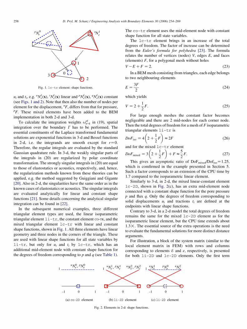
Fig. 1. lc-tr element: shape functions.


ui and ti, e.g.uNf

eðxÞ,tNf

eðxÞ linear andpNf

eðxÞ,qNf

eðxÞ constant

(see Figs. 1 and 2). Note that then also the number of nodes per

element for the displacement, uF, differs from that for pressure,pF. These mixed elements have been added to the BEM

implementation in both 2-d and 3-d.

To calculate the integration weights uefnKk in (19), spatial

integration over the boundary G has to be performed. The

essential constituents of the Laplace transformed fundamental

solutions are exponential functions in 3-d and Bessel functions

in 2-d, i.e. the integrands are smooth except for rZ0.

Therefore, the regular integrals are evaluated by the standard

Gaussian quadrature rule. In 3-d, the weakly singular parts of

the integrals in (20) are regularized by polar coordinate

transformation. The strongly singular integrals in (20) are equal

to those of elastostatics or acoustics, respectively, and, hence,

the regularization methods known from these theories can be

applied, e.g. the method suggested by Guiggiani and Gigante

[20]. Also in 2-d, the singularities have the same order as in the

known cases of elastostatics or acoustics. The singular integrals

are evaluated analytically for linear and constant shape

functions [21]. Some details concerning the analytical singular

integration can be found in [22].

In the subsequent numerical examples, three different

triangular element types are used, the linear isoparametric

triangular element li-tr, the constant element CO-TR, and the

mixed triangular element lc-tr with linear and constant

shape functions, shown in Fig. 1. All three elements have linear

geometry and three nodes in the corners of the triangle. These

are used with linear shape functions for all state variables by

li-tr, but only for ui and ti by lc-tr, which has an

additional mid-element node with constant shape function for

the degrees of freedom corresponding to p and q (see Table 1).

Fig. 2. Elements in 2-d

The co-tr element uses the mid-element node with constant

shape function for all state variables.

The lc-tr element brings in an increase of the total

degrees of freedom. The factor of increase can be determined

from the Euler’s formula for polyhedra [23]. The formula

relates the number of vertices (nodes) V, edges E, and faces

(elements) F, for a polygonal mesh without holes

VKECF Z 2: (23)

In a BEMmesh consisting from triangles, each edge belongs

to two neighbouring elements

EZ3F

2(24)

which yields

V Z 2C1

2F: (25)

For large enough meshes the constant factor becomes

negligeable and there are 2 mid-nodes for each corner node.

Then the total degrees of freedom for a mesh of F isoparametric

triangular elements li-tr is

DoFiso Z 4 2C1

2F

� �z2F (26)

and for the mixed lc-tr element

DoFmixed Z 3 2C1

2F

� �CFz

5

2F: (27)

This gives an asymptotic ratio of DoFmixed/DofisoZ1.25,

which is comfirmed in the example presented in Section 5.

Such a factor corresponds to an extension of the CPU time by

1.7 compared to the isoparametric linear element.

Similarly to 3-d, in 2-d, the mixed linear-constant element

lc-2D, shown in Fig. 2(c), has an extra mid-element node

connected with a constant shape function for the pore pressure

p and flux q. Only the degrees of freedom corresponding to

solid displacements ui and tractions ti are defined at the

endpoints with linear shape functions.

Contrary to 3-d, in a 2-d model the total degrees of freedom

remains the same for the mixed lc-2D element as for the

isoparametric linear element, but the CPU time extends about

1.3!. The essential source of the extra operations is the need

to evaluate the fundamental solutions for more distinct distance

arguments.

For illustration, a block of the system matrix (similar to the

local element matrix in FEM) with rows and columns

corresponding to elements E and e, respectively, is presented

for both li-2D and lc-2D elements. Only the first term

: shape functions.

Table 1

Element types

Element uNfe,

tNfe;

pNfe,

qNfe;

li-2D, li-tr Linear Linear

lc-2D, LC-TR Linear Constant


(i.e. with U, P and t, q) on the right hand side in Eq. (19) is

included as example, as the other one (with T, Q and u, p) is

analogical. Note that depending on the boundary condition

corresponding to each degree of freedom (row in the block), uiresp. p is given and ti resp. q unknown or vice versa. The given

term contributes to the right hand side and the unknown one to the

system matrix. The block is in the case of the li-2D element

ue1nKkðU

sijðy

E1Þ; uN1eÞ Kue1

nKkðPsj ðy

E1Þ; pN1eÞ ue1

nKkðUsijðy

E1Þ; uN2eÞ Kue1

nKkðPsj ðy

E1Þ; pN2eÞ

ue1nKkðU

fi ðy

E1Þ; uN1eÞ Kue1

nKkðPfðyE1Þ; pN1

eÞ ue1nKkðU

fi ðy

E1Þ; uN2eÞ Kue1

nKkðPfðyE1Þ; pN2

eÞ

ue2nKkðU

sijðy

E2Þ; uN1eÞ Kue2

nKkðPsj ðy

E2Þ; pN1eÞ ue2

nKkðUsijðy

E2Þ; uN2eÞ Kue2

nKkðPsj ðy

E2Þ; pN2eÞ

ue2nKkðU

fi ðy

E2Þ; uN1eÞ Kue2

nKkðPfðyE2Þ; pN1

eÞ ue2nKkðU

fi ðy

E2Þ; uN2eÞ Kue2

nKkðPfðyE2Þ; pN2

eÞ

26666664

37777775

te1i

qe1

te2i

qe2

2666664

3777775 (28)

and for the lc-2D element

ue1nKkðU

sijðy

E1Þ; uN1eÞ ue1

nKkðUsijðy

E1Þ; uN2eÞ Kue1

nKkðPsj ðy

E1Þ; pN0eÞ

ue2nKkðU

sijðy

E2Þ; uN1eÞ ue2

nKkðUsijðy

E2Þ; uN2eÞ Kue2

nKkðPsj ðy

E2Þ; pN0eÞ

ue0nKkðU

fi ðy

E0Þ; uN1eÞ ue0

nKkðUfi ðy

E0Þ; uN2eÞ Kue0

nKkðPfðyE0Þ; pN0

eÞ

2664

3775

te1i

te2i

qe0

2664

3775 (29)

where yEf is the position of the fth node of element E and tefi , qef

are the nodal values at the fth node of element e. The Dt and kDtarguments are omitted for space reasons aswell as the x argument

of the fundamental solutions, which runs through the element e

when computing the integral for uefnKk in Eq. (20).

The dimension of the local matrix for the isoparametric

element in (28) is 2!ð2C1ÞZ6 (two nodes, each with one

unknown vector ti (2 DoFs) and one unknown scalar q (1 DoF))

and for the mixed in (29) it is 2!2C1Z5 (two end-nodes,

each with one unknown vector ti (2 DoFs) and one mid-node

with one unknown scalar q (1 DoF)). The difference in the local

matrix size is not directly connected to a difference in the

global number of degrees of freedom, as the values at endpoints

(or triangle corners in 3-d) are shared with the neighboring

element(s) and those at the mid-element nodes are not. The size

of the global matrix can be determined using the Euler’s

formula for polyhedra (23).

Table 2

Material data for soil

K,G[N/m2] [varrho], [varrho]f[kg/m3]

f

2.1!108, 9.8!107 1884, 1000 0.48

6. Comparison of the mixed elements to a 1-d analytical

solution

To validate the BEM program, a study comparing the BEM

results to the 1-d analytical solution has been done for the

compressible and incompressible models. The time response of

the analytical solution has been obtained with the CQM, i.e. for

both the BEM and the analytical solutions, the same time

approximation is used. The material constants for the water

saturated coarse sand, i.e. a soil, are given in Table 2. For this

comparison, the Poisson’s ratio of the solid frame n is set to 0

resulting in different Young’s and shear moduli KZ8.5!107

and GZ1.3!108, respectively. Note that this only disables the

lateral contraction for the long-time (drained) material

behavior. For the short-time response (undrained), nus0 and

lateral contraction still plays a role.

For the geometry simulating the 1-d column in 2-d and 3-d,

see Figs. 3 and 4. The column is 3 m high, 1 m wide, and, in 3-

d, 1 m deep. On the top, it is excited by a traction jump

according to a unit step function ty(x,t)Z1 N/m2 H(t). The top

surface with load is permeable and all the remaining surfaces,

i.e. the sides and the vertically supported bottom, are

impermeable. On the sides, only sliding along the surface is

allowed, and movements in the perpendicular direction are

blocked.

In 2-d, the BEM model of the column described above

consists of 32 nodes and 32 elements, as shown in Fig. 3. A

finer discretization has 128 nodes and 128 elements. It will be

shown that the problem can be solved with the BEM

implementation.

In 3-d, the BEM model of the column described above

consists of 252 linear triangular elements on 128 nodes (see

Fig. 4(b)). The finer mesh in Fig. 4(c) has 700 elements and 352

R[N/m2] a k[m4/Ns]

1.2!109 0.981 3.55!10-9

Fig. 3. Comparison to 1-d analytical solution: 2-d geometry and discretization.


nodes. As in 2-d, the tests have shown that the results converge

to the analytical solution. However, it should be noted that the

finer 3-d mesh divides the edge of 1 m length in 5 element

lengths, whereas the coarse 2-d mesh has 4 elements on the

same length. Unfortunately, a finer 3-d mesh could not be

calculated on the computer used. Therefore, when comparing

with the 2-d results, it can be expected that the finer 3-d

discretization with 700 elements produces results comparable

to those from the coarse 2-d mesh with 32 elements.

In the subsequent study, the legend of the figures will point

to the element type with respect to the notation used in Table 1

and if an additional number is given, e.g. 128, it denotes the

number of elements used in the mesh.

Note that, as in other BEM implementations, there is a lower

stability limit, i.e. a minimum time step length condition for a

stable numerical solution in contrast to conditionally stable

Finite Differences schemes or Finite Elements, where usually

an upper limit on the time step length exists. This lower limit

here is determined by numerical tests with decreasing time step

size.

6.1. Results for compressible poroelasticity

Fig. 5(a) displays the displacement results at point P for the

finer mesh in 2-d and 3-d. The results in 2-d can not be

distinguished from each other and hardly from the analytical

solution.

Fig. 4. Comparison to 1-d analytical solut

The mixed linear-constant element brings a small improve-

ment in the lower stability limit on the timestep over the linear

isoparametric element. The optimal timestep on the coarser

mesh is DtZ0.00011 s compared to the DtZ0.00012 s for

linear isoparametric. For the constant element, the optimal

timestep isDtZ0.00033 s. On the finer mesh,DtZ2.5!10K5 s

has been used for all elements.

In 3-d, the optimal time steps used on the coarse 252

element mesh are DtZ0.0003 s for the li-tr element, DtZ0.0004 s for the LC-TR element, and DtZ0.0005 s for the co-tr element. For the finer mesh, an identical timestep, DtZ0.0002 s, has been chosen for both the linear and mixed

elements, and DtZ0.0004 s for the constant element. The

linear element allows the shortest timestep and comes closest

to the analytical solution.

The pore pressure behavior in Fig. 5(b) is essentially the

same as for the displacements, giving almost identical results

for the li-2D and lc-2D elements. Considering the pressure

results, the coarse mesh (3-d) is obviously a too crude

approximation for this material, not being able to resolve the

jumps sharply. The results for the finer mesh (2-d) look

noticeably better, clearly converging to the analytical solution.

Again, the mixed element has no advantages over the

isoparametric linear in 3-d.

6.2. Results for incompressible poroelasticity

If the same problem is considered for a material with

incompressible constituents, the solution changes (see also

[24]). The vibration corresponding to the fast compressional

wave disappears, which means the behavior is now governed

predominantly by the relative fluid to solid movement, because

the shear deformations should not play any significant role in

this 1-d setup. In Section 7, the two models will be tested and

compared on a more realistic example.

The displacement uy at the top surface and the pore pressure

p at the support are plotted against time in Fig. 6 for the finer

meshes.

In 2-d, the optimal timesteps used on the coarser mesh with

32 elements are DtZ0.0002 s for the linear and DtZ0.00015 s

for the mixed and constant elements. When the timestep

is made shorter (but not under the stability limit), i.e.

ion: 3-d geometry and discretization.

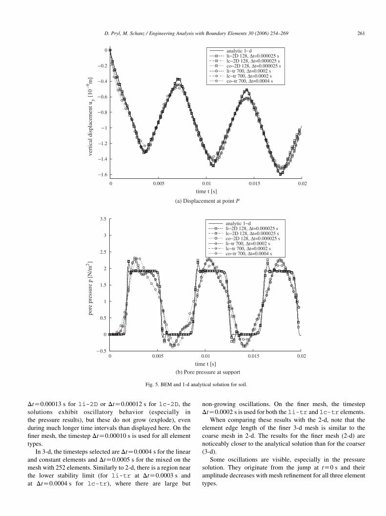
Fig. 5. BEM and 1-d analytical solution for soil.


DtZ0.00013 s for li-2D or DtZ0.00012 s for lc-2D, thesolutions exhibit oscillatory behavior (especially in

the pressure results), but these do not grow (explode), even

during much longer time intervals than displayed here. On the

finer mesh, the timestep DtZ0.00010 s is used for all element

types.

In 3-d, the timesteps selected are DtZ0.0004 s for the linear

and constant elements and DtZ0.0005 s for the mixed on the

mesh with 252 elements. Similarly to 2-d, there is a region near

the lower stability limit (for li-tr at DtZ0.0003 s and

at DtZ0.0004 s for lc-tr), where there are large but

non-growing oscillations. On the finer mesh, the timestep

DtZ0.0002 s is used for both the li-tr and lc-tr elements.

When comparing these results with the 2-d, note that the

element edge length of the finer 3-d mesh is similar to the

coarse mesh in 2-d. The results for the finer mesh (2-d) are

noticeably closer to the analytical solution than for the coarser

(3-d).

Some oscillations are visible, especially in the pressure

solution. They originate from the jump at tZ0 s and their

amplitude decreases with mesh refinement for all three element

types.

Fig. 6. BEM and 1-d analytical solution for incompressible soil.


For this problem, the mixed element offers a slightly better

stability limit over the isoparametric linear element in 2-d. It

also shows less oscillatory behavior when getting close to the

limit. In 3-d, as in all previous 3-d cases, the mixed element is

worse than the linear.

6.3. Comments on the validation

For all element types in both 2-d and 3-d, the results appear

to converge to the 1-d analytical solution as the mesh is refined.

The discretization used in the 3-d case is coarser compared to

that in 2-d with an element edge length of 1/4 versus 1/3 m on

the coarser mesh and 1/16 m versus 1/5 m on the finer mesh,

respectively. As expected, the 2-d results are closer to the

analytical solution.

In 2-d, the mixed elements bring minor improvements over

the isoparametric in terms of stability and result quality. In 3-d,

the mixed elements do not bring any improvements. They

produce worse results and have a narrower stability region than

the isoparametric.

Both was confirmed by tests with another material (a porous

rock, Berea sandstone; not included in this article, see [22]).

Fig. 7. 2-d column: Geometry, boundary conditions, and discretization.

Fig. 8. Results for t


In the case of the incompressible rock, the mixed element

offers clearly better stability over the linear one in 2-d.

However, the incompressible model is not a good description

of this material.

The difference between the numerical behavior of the mixed

elements in 2-d and 3-d demands a comment. One of the

possible reasons for different behavior of the element types in

2-d versus 3-d are the different approaches to singular

integration. In 2-d, the singular parts of the integrals are

computed analytically, whereas in 3-d, they are evaluated

numerically. Another, probably more important difference is in

the total degrees of freedom. Whereas there is no element type

dependent difference in the 2-d examples, in 3-d, there are

more nodes for constant approximation (mid-nodes) than for

he 2-d column.


linear (element corners). This leads to additional degrees of

freedom if some quantity is approximated with a lower degree

shape function.

If this is the main reason for the differences, it may be

interesting to implement and test mixed linear-constant

quadrilateral boundary elements (4 corner nodes, 1 mid-

element node) where the ratio DoFmixed/DoFiso is asymptoti-

cally 1, i.e. the same as for the lc-2D element in 2-d.

Elements combining quadratic and linear shape functions may

be of even more interest, as DoFmixed/DoFiso is always less than

1 if the nodes connected with lower order shape functions are a

subset of the higher order nodes.

Fig. 9. Compressible and inc

The result of the comparison may also depend slightly on

the choice of dimensionless variables (see Section 4.1).

However, no clear dependency has been recognized during

the tests.

7. Comparison of isoparametric and mixed elements in 2-d

and 3-d

In order to investigate the differences between the two

element types, now a more realistic poroelastic column is

considered in 2-d and 3-d. The material data correspond to the

ompressible 2-d column.


same water saturated coarse sand (soil) as before but here

the realistic Poisson’s ration (ns0) is used (see Table 2). Also,

the poroelastic column of 3 m length is fixed at the base and

traction-free on the sides. Further, it is loaded with a vertical

force on the top surface, as shown in Figs. 7 and 11. The

support is modeled impermeable (flux qZ0), all other surfaces

are permeable (pore pressure pZ0). Notice that unlike in

Section 6, displacements in direction(s) perpendicular to the

load are now possible, which allows lateral contraction and

waves based on shear to play a role. This makes the column

much more deformable (note the different scale in the results of

both time and displacements).

Fig. 10. Incompressi

7.1. Numerical example: 2-d poroelastic column

To compare the numerical behavior of the implemented

element types, first, a 2-d poroelastic column (3 m!1 m) is

considered (see Fig. 7). The used BEM discretizations are the

same as in Section 6.

The Fig. 8(a) show the displacement uy at the column

surface midpoint and the pore pressure p at the column base

midpoint, respectively, plotted against time for the li-2D,lc-2D, and co-2D elements. On the coarser mesh, the

optimal timestep has been chosen for each element type. The

stability region is slightly larger for the lc-2D element on

ble 2-d column.


the mesh with 32 elements: DtZ0.00017 s compared to

0.00018 s for li-2D. The results for the finer mesh have

been computed with the same timestep DtZ0.00005 s for all

element types. As there are no visible differences, only the li-2D element results are presented for the finer mesh. In the pore

pressure solution in Fig. 8(b), some oscillations arise with the

arrival of the fast compressional wave (the first non-zero

pressure value) induced by the load application at tZ0 s. They

are damped and have completely dissipated at about tZ0.02 s.

As described in Section 5, with the linear isoparametric

element all the state variables are localized at the geometry

nodes, i.e. the element end-nodes. For the mesh with 32

elements in Fig. 7, this gives 3!32Z96 total degrees of

freedom in the case of the li-2D element. The mixed linear-

constant element defines the solid displacement ui (resp.

traction ti) at the end-nodes and has an extra mid-node for the

pore pressure p (resp. flux q), which yields in total 2!32C1!32Z96 degrees of freedom. Thus, the total number of

degrees of freedom is the same for the linear and mixed

elements (this will be different later in the 3-d example).

Nevertheless, the CPU time needed extends about 1.3!. The

essential source of the extra operations is the need to evaluate

the fundamental solutions for more distinct distance argu-

ments. Clearly, the mixed element does not offer advantages

that would be worth the extra computational cost.

Now the incompressible model will be considered. Fig. 9

shows the displacement uy at point P on the top surface and the

pore pressure p in the middle of the support for the

compressible and incompressible models. Unlike the validation

example in chapter 6, there are no large differences between the

compressible and incompressible models of soil. That is due to

the boundary conditions, which differ substantially from the

validation example.

However, the lower stability limits are not the same as in the

compressible case. In Fig. 10, for each element the

displacement resp. pressure results are displayed for the

optimal timestep, DtZ0.00039 s for the li-2D element,

DtZ0.00018 s for lc-2D, and DtZ0.0003 s for co-2D. Inthis case, the mixed element allows to achieve better results

than the linear isoparametric on the same mesh. On the finer

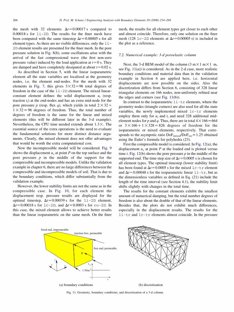
Fig. 11. Geometry, boundary conditions,

mesh, the results for all element types get closer to each other

and almost coincide. Therefore, only one solution on the finer

mesh (128 lc-2D elements at DtZ0.00005 s) is included in

the plot as a reference.

7.2. Numerical example: 3-d poroelastic column

Next, the 3-d BEM model of the column (3 m!1 m!1 m,

see Fig. 11(a)) is considered. As in the 2-d case, more realistic

boundary conditions and material data than in the validation

example in Section 6 are applied here, i.e. horizontal

displacements are now possible on the sides. Also the

discretization differs from Section 6, consisting of 328 linear

triangular elements on 166 nodes, non-uniformly refined near

the edges and corners (see Fig. 11(b)).

In contrast to the isoparametric li-tr elements, where the

geometry nodes (triangle corners) are also used for all the state

variables, the newly implemented mixed lc-tr elements

employ them only for ui and ti and need 328 additional mid-

element nodes for p and q. Thus, there are in total 4!166Z664

or 3!166C1!328Z826 degrees of freedom for the

isoparametric or mixed elements, respectively. That corre-

sponds to the asympotic ratio DoFmixed/DoFisoZ1.25 obtained

using the Euler’s formula for polyhedra (23).

First the compressible model is considered. In Fig. 12(a), the

displacement uy at point P at the loaded end is plotted versus

time t. Fig. 12(b) shows the pore pressure p in the middle of the

supported end. The time step size of DtZ0.0005 s is chosen for

all element types. The optimal timestep (lower stability limit)

has been found at DtZ0.0005 s for the mixed lc-tr element

and DtZ0.00048 s for the isoparametric linear li-tr, but asthe dimensionless variables as defined in Eq. (21) include the

length of the time interval (see Section 4.1), the stability limit

shifts slightly with changes in the total time.

The results for the constant elements exhibit the smallest

amount of numerical damping, but the total number degrees of

freedom is also about the double of that of the linear elements.

Besides that, the plots do not exhibit much differences,

especially in the displacement results. The results for the

li-tr and lc-tr elements almost coincide. In the pressure

and discretization of a 3-d column.

Fig. 12. Compressible 3-d column.


plot, a small difference in favor of the mixed element which

shows less numerical damping can be observed. On the other

hand, there is the disadvantage in the lower stability limit.

None of the differences can be considered substantial.

At the same time, the total number of the degrees of freedom

increased by a factor of 1.25, resulting in longer computation

time by a factor of about 1.7, which corresponds to the

quadratic dependence between the degrees of freedom and the

number of operations. Clearly, there are no improvements that

would offset this extra computational cost of the mixed

element.

Now, the results of the incompressible model will be

considered. In Figs. 13(a) and 13(b), the displacement and the

pore pressure for the compressible and incompressible models

are compared for the linear element and timestep length DtZ0.0005 s.

Unlike the test in chapter 6, there are no noticeable

differences between the models with compressible and

incompressible constituents. On the mesh used, the differences

between the models are of the same order as those between the

element types. There is also no difference in the stability region

compared to the compressible model.

Fig. 13. Compressible and incompressible 3-d column.


8. Conclusions

Mixed linear-constant elements have been implemented in

both 2-d and 3-d BEM. The poroelastodynamic BEM

implementation is tested on examples representing a 1-d

problem in both 2-d and 3-d. It approximates the 1-d analytical

solution very well. For this verification example and additional,

more realistic problems, the results are compared to those of

isoparametric linear elements.

In 2-d, the difference in CPU time is extended by a factor of

1.3 compared to the linear isoparametric elements. For the

compressible model, the (negligibly) shorter possible time step

does not bring any noticeable improvement to the results. The

difference is more pronounced for the incompressible model,

where the mixed element, in at least some cases, offers a

considerable reduction of the lower stability limit and reduces

the oscillatory behavior near the limit.

In most of the 3-d tests, the mixed elements performed

worse than the isoparametric elements with regard to both the

quality of numerical results and the stability. In some tests,

minor improvements are observed in the quality of numerical

results, but the computation time extends by a factor of 1.7 due

to the increase in the total degrees of freedom. In this case, the

advantages clearly do not correspond to the increased


computational cost, as one can achieve better results with the

same effort using a finer discretization and linear isoparametric

elements. This corresponds to the conclusions in the Ref. [7].

Acknowledgements

The authors gratefully acknowledge the financial support by

the German Research Foundation (DFG) under grant SCHA

527/5-2.

References

[1] Schanz M. Wave propagation in viscoelastic and poroelastic continua: a

boundary element approach Lecture notes in applied mechanics. Berlin:

Springer; 2001.

[2] Cheng AH-D, Badmus T, Beskos D. Integral equations for dynamic

poroelasticity in frequency domain with BEM solution. J Eng Mech

ASCE 1991;117(5):1136–57.

[3] Manolis G, Beskos D. Integral formulation and fundamental solutions of

dynamic poroelasticity and thermoelasticity. Acta Mech 1989;76:89–104

[errata [25]].

[4] Chen J, Dargush G. Boundary element method for dynamic poroelastic

and thermoelastic analysis. Int J Solids Struct 1995;32(15):2257–78.

[5] Schanz M. Application of 3-d boundary element formulation to wave

propagation in poroelastic solids. Eng Anal Bound Elem 2001;25(4–5):

363–76.

[6] Lewis R, Schrefler B. The finite element method in the static and dynamic

deformation and consolidation of porous media. Chichester: Wiley; 1998.

[7] Steinbach O. Mixed approximations for boundary elements. J Numer

Anal SIAM 2000;38:401–13.

[8] Biot M. General theory of three-dimensional consolidation. J Appl Phys

1941;12:155–64.

[9] Biot M. Theory of propagation of elastic waves in a fluid-saturated porous

solid. I. Low-frequency range. J Acoust Soc Am 1956;28(2):168–78.

[10] Bonnet G, Auriault J-L. Dynamics of saturated and deformable porous

media: Homogenization theory and determination of the solid-liquid

coupling coefficients. In: Boccara N, Daoud M, editors. Physics of finely

divided matter. Berlin: Springer; 1985. p. 306–16.

[11] Biot M. Theory of propagation of elastic waves in a fluid-saturated

porous solid.II. higher frequency range. J Acoust Soc Am 1956;28(2):

179–91.

[12] Bonnet G. Basic singular solutions for a poroelastic medium in the

dynamic range. J Acoust Soc Am 1987;82(5):1758–62.

[13] Detournay E, Cheng AH-D. Fundamentals of poroelasticity. In:

Comprehensive rock engineering: principles, practice and projects, vol.

II. New York: Pergamon Press; 1993. p. 113–71 [chapter 5].

[14] Schanz M, Pryl D. Dynamic fundamental solutions for compressible and

incompressible modeled poroelastic continua. Int J Solids Struct 2004;

41(15):4047–73.

[15] Domınguez J. Boundary element approach for dynamic poroelastic

problems. Int J Numer Method Eng 1992;35(2):307–24.

[16] Lubich C. Convolution quadrature and discretized operational calculus.

I/II. Numer Math 1988;52:129–45 [see also p. 413–425].

[17] Schanz M, Antes H. Application of ‘operational quadrature methods’ in

time domain boundary element methods. Meccanica 1997;32(3):

179–86.

[18] Schanz M. A boundary element formulation in time domain for

viscoelastic solids. Commun Numer Method Eng 1999;15:799–809.

[19] Kielhorn L. Modellierung von wellenausbreitung in porosen boden:

Dimensionslose variablen fur eine randelementformulierung. Diplomar-

beit. Technische Universitat Braunschweig, Institut fur Angewandte

Mechanik, Fachbereich Bauingenieurwesen; 2004.

[20] Guiggiani M, Gigante A. A general algorithm for multidimensional

cauchy principal value integrals in the boundary element method. J Appl

Mech ASME 1990;57:906–15.

[21] Telles J. Elastostatic problems. In: Brebbia C, editor. Topics in boundary

element research. Computational aspects, vol. 3. Berlin: Springer; 1987.

p. 265–94.

[22] Pryl D. Influences of poroelasticity on wave propagation: a time stepping

boundary element formulation. Braunschweig series on mechanics, vol.

58. Technical University Braunschweig; 2005.

[23] de Berg M, van Kreveld M, Overmars M, Schwarzkopf O.

Computational geometry algorithms and applications. 2nd ed. Berlin:

Springer; 2000.

[24] Schanz M, Diebels S. A comparative study of biot’s theory and the linear

theory of porous media for wave propagation problems. Acta Mech 2003;

161(3–4):213–35.

Comparison of mixed and isoparametric boundary elements in time domain poroelasticity

Documents