Multivariate Behavioral Research, 46:779–811, 2011 Copyright © Taylor & Francis Group, LLC ISSN: 0027-3171 print/1532-7906 online DOI: 10.1080/00273171.2011.606748 Comparison of Methods for Collecting and Modeling Dissimilarity Data: Applications to Complex Sound Stimuli Bruno L. Giordano and Catherine Guastavino McGill University Emma Murphy Dublin City University Mattson Ogg, Bennett K. Smith, and Stephen McAdams McGill University Sorting procedures are frequently adopted as an alternative to dissimilarity ratings to measure the dissimilarity of large sets of stimuli in a comparatively short time. However, systematic empirical research on the consequences of this experiment- design choice is lacking. We carried out a behavioral experiment to assess the extent to which sorting procedures compare to dissimilarity ratings in terms of efficiency, reliability, and accuracy, and the extent to which data from different data-collection methods are redundant and are better fit by different distance models. Participants estimated the dissimilarity of either semantically charged environmental sounds or semantically neutral synthetic sounds. We considered free and hierarchical sorting and derived indications concerning the properties of constrained and truncated hierarchical sorting methods from hierarchical sorting data. Results show that the higher efficiency of sorting methods comes at a considerable cost in terms of data reliability and accuracy. This loss appears to be minimized with truncated hierarchical sorting methods that start from a relatively low number of groups of stimuli. Finally, variations in data-collection method Correspondence concerning this article should be addressed to Bruno L. Giordano, Schulich School of Music, McGill University, 555 Sherbrooke Street West, Montréal, Québec, Canada H3A 1E3. E-mail: [email protected] 779 Downloaded by [McGill University Library] at 11:08 31 January 2012

Welcome message from author
This document is posted to help you gain knowledge. Please leave a comment to let me know what you think about it! Share it to your friends and learn new things together.
Transcript

Multivariate Behavioral Research, 46:779–811, 2011
Copyright © Taylor & Francis Group, LLC
ISSN: 0027-3171 print/1532-7906 online
DOI: 10.1080/00273171.2011.606748
Comparison of Methods for Collectingand Modeling Dissimilarity Data:
Applications to Complex Sound Stimuli
Bruno L. Giordano and Catherine GuastavinoMcGill University
Emma MurphyDublin City University
Mattson Ogg, Bennett K. Smith, and Stephen McAdamsMcGill University
Sorting procedures are frequently adopted as an alternative to dissimilarity ratings
to measure the dissimilarity of large sets of stimuli in a comparatively short time.
However, systematic empirical research on the consequences of this experiment-
design choice is lacking. We carried out a behavioral experiment to assess the
extent to which sorting procedures compare to dissimilarity ratings in terms of
efficiency, reliability, and accuracy, and the extent to which data from different
data-collection methods are redundant and are better fit by different distance
models. Participants estimated the dissimilarity of either semantically charged
environmental sounds or semantically neutral synthetic sounds. We considered
free and hierarchical sorting and derived indications concerning the properties of
constrained and truncated hierarchical sorting methods from hierarchical sorting
data. Results show that the higher efficiency of sorting methods comes at a
considerable cost in terms of data reliability and accuracy. This loss appears to be
minimized with truncated hierarchical sorting methods that start from a relatively
low number of groups of stimuli. Finally, variations in data-collection method
Correspondence concerning this article should be addressed to Bruno L. Giordano, Schulich
School of Music, McGill University, 555 Sherbrooke Street West, Montréal, Québec, Canada H3A
1E3. E-mail: [email protected]
779
Dow
nloa
ded
by [
McG
ill U
nive
rsity
Lib
rary
] at
11:
08 3
1 Ja
nuar
y 20
12

780 GIORDANO ET AL.
differentially affect the fit of various distance models at the group-average and
individual levels. On the basis of these results, we suggest adopting sorting as an
alternative to dissimilarity-rating methods only when strictly necessary. We also
suggest analyzing the raw behavioral dissimilarities, and avoiding modeling them
with one single distance model.
Similarity is a fundamental construct in the empirical and theoretical study of
a variety of cognitive and perceptual processes such as categorization, prob-
lem solving, generalization, and memory retrieval (Goldstone, 1999; Shepard,
1987; Tversky, 1977). Various distance models are available to model dissim-
ilarities as a function of the features of the judged stimuli (Tversky, 1977; for
differences between similarity and dissimilarity judgments, see Gati & Tversky,
1982; Tversky & Gati, 1978), and empirical studies often aim to measure the
features underlying the mental representation of the stimuli (for exploratory
and confirmatory approaches, see Borg & Groenen, 1997). Dissimilarities can
be collected with various methods (e.g., Henry & Stumpf, 1975; Rao & Katz,
1971; Tsogo, Masson, & Bardot, 2000). Although several studies have quantified
the merits and disadvantages of the various data-collection methods, none has
jointly considered all the factors relevant to their comparison: their efficiency, the
reliability and accuracy of the data, the similarity of data collected with different
methods (redundancy), and the effects of method on the fit of distance models.
As a consequence, the methods-comparison literature is widely scattered, and
several of these aspects remain partially investigated, at best. We investigated
the extent to which the previously mentioned factors vary across data-collection
methods. We considered the methods of dissimilarity ratings, hierarchical sort-
ing, and free sorting, and modeled the properties of the constrained and truncated
hierarchical sorting methods from the hierarchical sorting data.
Among the various methods, that of dissimilarity ratings or paired com-
parisons is perhaps the most popular. Accordingly, participants rate along a
categorical or continuous scale the dissimilarity of each of the N.N � 1/=2
possible pairs of N stimuli. Despite its popularity, this method is regarded as
relatively inefficient because it requires a large number of judgments that grows
quadratically with the set size (Rosenberg & Kim, 1975). Further, the inefficiency
of this method makes it unsuitable for perceptual domains subject to considerable
carryover and adaptation effects (e.g., tastes and smells; Lawless, Sheng, &
Knoops, 1995). The inefficiency of this method also makes it prohibitive for in-
vestigating large sets of stimuli because the required long experimental sessions
would result in fatigue and boredom (Bijmolt & Wedel, 1995; M. D. Johnson,
Lehmann, & Horne, 1990; Malhotra, 1990) and in uncontrolled fluctuations of
the response criteria throughout the experimental session. A number of studies
investigated more efficient variants of this method that produce incomplete
dissimilarity matrices (e.g., Tsogo et al., 2000). Interestingly, an input spatial
Dow
nloa
ded
by [
McG
ill U
nive
rsity
Lib
rary
] at
11:
08 3
1 Ja
nuar
y 20
12

COMPARISON OF METHODS 781
representation can be accurately recovered through a multidimensional scaling
(MDS) analysis of the incomplete dissimilarity matrix, provided that at least
two-thirds of the data are available (Spence & Domoney, 1974) or that only
dissimilarities of intermediate magnitude are not available (Graef & Spence,
1979). For these reasons, incomplete designs are of limited value: they rely on
the assumption that data can indeed be accurately represented with an MDS
model, they require preliminary estimates of the entire dissimilarity matrix
necessary to identify dissimilarities of intermediate magnitude, and they reduce
the experimentation time by only 33%, at best.
Sorting methods are a widely adopted alternative to dissimilarity ratings. With
sorting methods, participants create groups of similar stimuli (Coxon, 1999; for
cognitive theories on the relationship between similarity and categorization, see
Goldstone, 1994). With free sorting (Miller, 1969; Rosenberg & Kim, 1975),
participants are free to decide on how many groups they should create, whereas
with constrained sorting the number of groups is fixed by the experimenter. For
both of these methods, a binary dissimilarity is derived from the cooccurrence
of the stimuli within the groups (dissimilarity D 0 and 1 if two stimuli are in the
same group or not, respectively). The variant of hierarchical sorting (hierarchy-
construction method, Harloff & Coxon, 2005; successive sorting method, Bimler
& Kirkland, 1997) is the behavioral analog of the hierarchical clustering scheme
(S. C. Johnson, 1967). With agglomerative hierarchical sorting, participants start
from a condition in which each of the stimuli is in a different group and, at
each subsequent step, merge together the two most similar stimuli or groups
of stimuli until all stimuli are merged together. Dissimilarity can be measured
as N minus the number of groups into which the stimulus set is partitioned at
the moment the two stimuli are first merged (Rao & Katz, 1971). Variants of
this method are available: divisive hierarchical sorting proceeds in the direction
opposite to that of agglomerative hierarchical sorting, starting from the one-
group condition (Boster, 1986); truncated agglomerative hierarchical sorting
starts with a constrained sorting phase (number of groups < N ; Harbke, 2003)
or with a free-sorting phase (Bimler, Kirkland, & Chen, 1998).
The comparative study of dissimilarity ratings and sorting methods has been
fragmentary. The choice of a data-collection method should take into account
various factors: method efficiency, data reliability (the extent to which results
can be replicated either with the same participants or with a different group of
participants), and data accuracy (the extent to which data accurately reflect the
features of the investigated stimuli); method redundancy (the extent to which
different methods yield comparable data); and data-modeling biases (the extent
to which data from a given method are optimally accounted for by a particular
distance model). To date, no study has jointly considered all these factors, thus
making the process of selecting a method difficult at best or uninformed at worst.
For example, free sorting is often chosen on the grounds that it is a very efficient
Dow
nloa
ded
by [
McG
ill U
nive
rsity
Lib
rary
] at
11:
08 3
1 Ja
nuar
y 20
12

782 GIORDANO ET AL.
alternative to dissimilarity ratings (e.g., in Bijmolt & Wedel, 1995; free sorting
is 2.5 times faster than dissimilarity ratings). However, the price of the increased
efficiency is seldom considered: for example, free sorts are known to be less
accurate than dissimilarity ratings (Subkoviak & Roecks, 1976). Further, other
differences between free sorting and dissimilarity ratings are simply unknown: no
study has compared their reliability, and redundancy studies (Bertino & Lawless,
1993; Bonebright, 1996; Cartier et al., 2006; Ward, 1977) are often carried out by
focusing on MDS models, rather than on raw data (for an exception, see Harbke,
2003), despite the known inaccuracies of the MDS analysis of the binary free-
sorting dissimilarities (Goodhill, Simmen, & Willshaw, 1995; Kendall, 1975;
Simmen, 1996) and the vulnerability of the fit of these models to variations in
the distributional properties of the input data (Pruzansky, Tversky, & Carroll,
1982).
The methodological study of hierarchical sorting is even less developed. The
best-studied aspects are the redundancy and reliability of this method. When
compared with dissimilarity ratings, hierarchical sorts are thus reported to be
fairly redundant (Bricker & Pruzansky, 1970; Harbke [2003] reported a correla-
tion of .60 between group-average truncated hierarchical sorts and dissimilarity
ratings), but are also characterized by a larger degree of interindividual differ-
ences (Bricker & Pruzansky, 1970; for the effects of the number of participants
on the correlation between group-average hierarchical sorts, see Griffiths &
Kalish, 2002). However, empirical data on other properties of this method
are lacking. For example, although Bimler and Kirkland (1997) stated that
hierarchical sorting cannot be used to investigate more than 16 items because of
its inefficiency, it is unknown whether this method still represents a more efficient
alternative to dissimilarity ratings. Focusing on data accuracy, Bimler & Kirkland
claimed that hierarchical sorts provide more information than free sorting (hi-
erarchical sorting dissimilarities can assume a larger number of different values
than can binary free-sorting dissimilarities). Consistently, Rao and Katz (1971)
showed that hierarchical sorting is the most accurate among a variety of sorting
methods. Note, however, that Rao & Katz (1971) investigated simulated and not
real behavioral data, and accuracy measures were computed from MDS solutions
rather than from the raw data. Finally, hierarchical sorting is claimed to be more
suitable for the quantification of interindividual differences than free sorting
(Lawless et al., 1995) and requires fewer participants than free sorting, but is also
claimed to be more demanding (Bimler & Kirkland, 1997). Notably, however,
no clear empirical data are available to substantiate either of these claims.
Empirical studies of dissimilarity often base their conclusions not on analyses
of the raw dissimilarity data, but on the parameters of a distance model of the raw
dissimilarities. Given the importance of this modeling step, experimenters may
be interested in assessing the extent to which model-based conclusions can be
replicated by studies based on different data-collection methods and, above all,
Dow
nloa
ded
by [
McG
ill U
nive
rsity
Lib
rary
] at
11:
08 3
1 Ja
nuar
y 20
12

COMPARISON OF METHODS 783
they may choose the method which generates data that are accurately accounted
for by the distance model of interest. For instance, an experimenter interested in
MDS models may choose the method whose data are better accounted by this
model. Thus, hierarchical sorts would be a less than optimal choice for MDS-
based studies because each individual yields an ultrametric tree (see Appendix)
that can be represented perfectly by a Euclidean space with a rather large number
of dimensions (N � 1; Holman, 1972; for additional considerations, see Carroll
& Pruzansky, 1980), but would likely be a reasonable choice if the modeling
interest is in graph-theoretic structures (e.g., additive trees; see Appendix).
In addition to these considerations, the experimenter may also be interested
in assessing the extent to which model-based conclusions can be replicated
by studies based on different data-collection methods. To our knowledge, no
previous empirical work has explored this important dimension of comparison
for the data-collection methods.
We carried out a comparative study of dissimilarity ratings, free sorting, and
agglomerative hierarchical sorting (referred to simply as hierarchical sorting
from now on). In order to increase the generality of the results, behavioral
dissimilarities were collected for two largely different sound sets: a semantically
neutral set of unrecognizable synthetic sounds and a semantically charged set of
recognizable living environmental sounds (Giordano, McDonnell, & McAdams,
2010). Data-collection methods were compared focusing on various factors
of potential interest to the experiment-design process: efficiency, reliability,
redundancy, data modeling, and accuracy. Results for each of these aspects are
discussed separately at the end of the relevant parts of the Results section. The
data-modeling analysis was complemented by a study of the influence of the
distributional properties of the data on model fit (Pruzansky et al., 1982). Var-
ious analyses considered truncated hierarchical sorting and constrained sorting
data derived from the hierarchical sorting data collected with the experimental
participants. The validity of the derived data was assessed when analyzing the
redundancy of data from different methods. Given their nature, the conclusions
reached for derived data should be taken as an indication of what might be
expected from an actual experiment based on these methods.
METHOD
Participants
Participants (N D 120; M D 23 years, SD D 4 years; 75 women, 45 men) were
native English speakers and had normal hearing, as assessed with a standard
audiometric procedure (International Organization for Standardization, 2004;
Martin & Champlin, 2000).
Dow
nloa
ded
by [
McG
ill U
nive
rsity
Lib
rary
] at
11:
08 3
1 Ja
nuar
y 20
12

784 GIORDANO ET AL.
Stimuli
We selected two sets of 20 stimuli each. The semantic set comprised highly
recognizable vocal and nonvocal living environmental sounds (Giordano et al.,
2010). The synthetic set comprised harmonic tones equalized in perceived du-
ration and loudness and differing in attack time, spectral centroid, and the
ratio between the levels of even and odd harmonics (Experiment 3, Caclin,
McAdams, Smith, & Winsberg, 2005). Each of the three variable parameters
had the same range of variation as in Caclin et al. (2005) and could assume one
of 20 different values, evenly spaced along a psychophysically linear scale. For
each stimulus, the level of the synthesis parameters was selected at random and
without replacement from the 20 available values. The sounds in the synthetic
set were perceptually more similar to each other than were those in the semantic
set, and none of them could be associated with a real-world sound-generating
event. We selected two 10-stimulus training sets that were different from the
experimental sets. The semantic set comprised five living and five nonliving
sounds. For the synthetic set, the three synthesis parameters varied within the
same range as for the experimental set.
Apparatus
Sound stimuli were stored on the hard disk of a Mac Pro Quad Core Workstation
equipped with an M-Audio CO2 optical-to-coaxial S/PDIF converter. Audio
signals were amplified with a Grace Design m904 monitor system and presented
through Sennheiser HD595 headphones. Participants were seated in a structurally
isolated, soundproofed room with a noise-floor rating of PNC20. Sound peak
level was 58 dB SPL on average (SD D 12 dB).
Design and Procedure
We adopted a 2 � 3 between-subjects design by combining two levels for the
sound set factor (semantic vs. synthetic set) with three levels for the data-
collection method factor (dissimilarity ratings, and hierarchical or free sorting).
Twenty participants were randomly assigned to each of the six cells of the
experimental design.
Before estimating the dissimilarities, participants were familiarized with the
stimuli by presenting them all twice in sequence in block-randomized order
(interstimulus-interval [ISI] D 100 ms). They were instructed to estimate the
maximum and minimum within-set dissimilarities while listening to the sounds.
The task of estimating the dissimilarities with one of the three investigated
methods began after this familiarization phase.
Dow
nloa
ded
by [
McG
ill U
nive
rsity
Lib
rary
] at
11:
08 3
1 Ja
nuar
y 20
12
COMPARISON OF METHODS 785
On each trial of the dissimilarity-rating condition, participants were presented
with one of the possible N.N � 1/=2 pairs of different sounds (N = number
of stimuli) and rated the dissimilarity of the sounds by moving a slider along
a scale marked “very similar” and “very different” at the two extremes. The
within-pair order was chosen at random on each trial.
In the first step of the hierarchical sorting condition, participants were pre-
sented with N randomly numbered on-screen icons corresponding to the N
sounds. Icons could be dragged around the screen by using the mouse. Partic-
ipants were asked to listen to each of the sounds by clicking on the icons and
to drop the two most similar sounds inside a merging box. When the merging
box contained two sounds, participants clicked on an on-screen button labeled
“OK” to create a new icon that pointed to the two grouped sounds. The new
icon was labeled with the numbers of the icons for the merged stimuli (e.g.,
3-6 for the merged icons 3 and 6). When the participant clicked on an icon
for merged sounds, all of the sounds were played back in random order (ISI D
100 ms). At each subsequent step of the procedure, participants were asked to
drop the two most similar sounds or groups of sounds inside the merging box.
Participants were required to listen to each of the stimuli at least once before
each of the first three merging decisions. The procedure ended when only two
groups of stimuli remained to be merged.
In the free sorting condition, participants were presented with N randomly
numbered on-screen icons, one for each of the N stimuli. They were asked to
create as many nonempty groups of similar sounds as they thought necessary,
but not less than two groups and not more than N � 1. Sounds were grouped by
dropping the icons inside a merging box, one for each of the groups. Participants
were required to listen to each of the sounds at least twice before creating any
group and to listen to each of the groups at least once after each of the sounds
had been dropped inside one of the merging boxes.
In all conditions, participants could listen to the stimuli as many times as
needed before giving a response. At the beginning of the hierarchical and
free-sorting tasks, participants were required to arrange the on-screen icons
so that similar sounds were closer together. Participants were told that this
initial step was meant to aid the process of creating groups of sounds and
were instructed to start grouping the sounds that they had arranged closer on
the screen. In all conditions, response-related operations (e.g., drag the icons
or move the slider) were also possible during the playback of the sounds.
For all of the conditions, the task was initially practiced with the training
set. For the training phase (M duration D 6.5 min; SD D 4:2 min), partic-
ipants rated the dissimilarity of 10 pairs randomly selected out of the pos-
sible 45, or carried out the previously described sorting procedures in their
entirety.
Dow
nloa
ded
by [
McG
ill U
nive
rsity
Lib
rary
] at
11:
08 3
1 Ja
nuar
y 20
12

786 GIORDANO ET AL.
TABLE 1
Temporal Factors for the Data-Collection Methods and Sound Sets
Averaged Across Participants
Semantic Set Synthetic Set
DR HS FS DR HS FS
Method M SE M SE M SE M SE M SE M SE
Experiment duration (min) 33.09 1.77 25.70 1.75 14.66 0.61 21.18 1.65 17.39 1.33 17.18 1.91
Playback time (min) 18.76 1.26 14.88 1.22 4.77 0.28 7.21 0.66 5.65 0.52 3.94 0.71
Nonplayback time (min) 14.33 0.91 10.82 0.61 9.90 0.53 13.97 1.11 11.74 0.87 13.24 1.36
Number of playbacks 23.05 1.55 18.40 1.51 5.96 0.36 33.96 3.11 27.11 2.51 19.28 3.41
Note. DR D dissimilarity ratings; HS D hierarchical sorting; FS D free sorting.
RESULTS
All analyses considered group-average data. Individual data were considered in
the data-modeling and accuracy analyses. The minimum and maximum possible
dissimilarity ratings were 0 and 1, respectively. With hierarchical sorting, the
dissimilarity of two stimuli was computed as 1 � Ng=N [range: 1/N to .N �
1/=N ], where Ng is the number of groups into which the stimulus set is
partitioned at the moment the two stimuli are first merged (Rao & Katz, 1971).
With free sorting, the (binary) dissimilarity of two stimuli equals 0 if the stimuli
are grouped together and 1 if they are not. For each of the hierarchical sorting
steps, differing in the number of groups of stimuli, we finally computed a binary
dissimilarity following the same cooccurrence approach as for the free-sorting
method. These distance matrices derived from the hierarchical sorting data are
taken as an approximation of real constrained sorting dissimilarities (see redun-
dancy analyses for validation). For all methods, group-average dissimilarities
were given by the average of individual data.1
Efficiency
Table 1 reports four different temporal measures for each of the experimental
conditions: experiment duration, playback time, nonplayback time dedicated
exclusively to response operations (Tresp), and number of playbacks/stimulus
(Nplays). None of these measures considered the initial phase of familiarization
with the stimuli. As shown in Table 1, the experiment took more time for the
1Hierarchical sorting dissimilarities are more rigorously conceptualized as ordinal measures and
should thus be pooled across participants using the median and not the mean. In the present study,
the Pearson correlation between median- and mean-pooled hierarchical sorting data is .95 and .97
for the semantic and synthetic sets, respectively.
Dow
nloa
ded
by [
McG
ill U
nive
rsity
Lib
rary
] at
11:
08 3
1 Ja
nuar
y 20
12

COMPARISON OF METHODS 787
semantic than for the synthetic set. This difference in part reflects a longer
average duration of the semantic sounds compared to the synthetic sounds,
2.4 s (SD D 1:24) and 0.6 s (SD D 0:01), respectively. Nplays was higher
for dissimilarity ratings than for hierarchical and free sorting. This difference
in part reflects the minimum number of playbacks required for each condition:
19 for dissimilarity ratings and 3 for hierarchical and free sorting. Within two
separate 2 � 3 analyses of variance (ANOVAs), we analyzed the influence of
sound set and data-collection method on both Tresp and Nplays. The interaction
between sound set and data-collection method was not significant for either
temporal factor, F.2; 114/ D 2:10 and 0.51, p D :13 and .60, ˜2p D :04 and
.01, for Tresp and Nplays, respectively. Data-collection method significantly
influenced both variables, F.2; 114/ D 5:91 and 25.17, p D :004 and < .001,
˜2p D :09 and .31, for Tresp and Nplays, respectively. Both variables were
higher with dissimilarity ratings than with both sorting methods: for Tresp as
dependent variable, unpaired t.78/ D 3:32 and 2.52, p D :002 and .01, for
hierarchical and free sorting, respectively; for Nplays as dependent variable,
unpaired t.78/ D 2:34 and 5.83, p D :02 and < .001, for hierarchical and free
sorting, respectively. Whereas Nplays was higher for hierarchical than for free
sorting, t.78/ D 4:03, p < :001, Tresp did not differ significantly between them,
t.78/ D �0:32, p D :75. Finally, whereas Nplays was lower for the semantic
than for the synthetic set, F.1; 114/ D 35:17, p < :001, ˜2p D :24, Tresp was not
reliably different for the two sound sets, F.1; 114/ D 50:89, p D :09, ˜2p D :03.
We created a model for predicting the amount of time necessary to evaluate
N stimuli with each of the following methods: dissimilarity ratings, free sorting,
hierarchical sorting, and truncated hierarchical sorting (see Figure 1). The model
extrapolates the empirical efficiency measures obtained with N D 20 stimuli to
various untested stimulus-set sizes. The reader should take the results of this
modeling as an indication of the experiment duration that requires a validation
through pilot experimental testing. Experiment duration was modeled as:
dissimilarity ratings
�
Tpres D Tstim N .N � 1 C k1/
Tresp D k2N .N � 1/ =2
hierarchical sorting
�
Tpres D Tstim N .3 C k1M/
Tresp D k2NM
free sorting
�
Tpres D Tstim N .3 C k1/
Tresp D k2N(1)
where Tpres is the presentation time for all stimuli, Tstim is the average stimulus-
presentation time, and M is the number of hierarchical sorting steps D number
of starting groups � number of groups after final merge (M D N � 1 for
complete hierarchical sorts that do not omit the last trivial step where all sounds
are grouped together; this trivial step was omitted from the simulations, and
Dow
nloa
ded
by [
McG
ill U
nive
rsity
Lib
rary
] at
11:
08 3
1 Ja
nuar
y 20
12

788 GIORDANO ET AL.
FIGURE 1 Estimates of experiment duration as a function of the size of the stimulus set
and data-collection method (average stimulus duration D 1 s). DR D dissimilarity ratings;
HS D hierarchical sorting; FS D free sorting; TSN=4 and TS5 D truncated HS with a number
of starting groups equal to one fourth of the number of stimuli and to five, respectively.
was not carried out in the behavioral experiments). We considered a minimum
Nplays of 3 for hierarchical and free sorting and of N � 1 for dissimilarity
ratings. These values correspond to those used in the actual experiment. The
constant k1 models the spontaneous Nplays beyond the minimum requirement
throughout the entire experiment for dissimilarity ratings and free sorting, and
for each of the hierarchical sorting steps. The constant k2 models Tresp for each
dissimilarity-rating pair or for each stimulus in free sorting or for each stimulus
in each of the hierarchical sorting steps. The constants k1 and k2 were estimated
from the empirical data and averaged across sound sets. Predictions were carried
out by assuming a stimulus duration of 1 s.
Based on this modeling approach, hierarchical and free-sorting methods do
not appear to be noticeably more efficient than dissimilarity ratings for a number
of stimuli lower than 30. For larger sets, free sorting appears instead to be an in-
creasingly more efficient alternative to both hierarchical sorting and dissimilarity
ratings. The comparative gain in efficiency of hierarchical sorting relative to dis-
similarity ratings is very small for any set size. Interestingly, truncated hierarchi-
cal sorting appears to be highly efficient even when compared with free sorting.
Dow
nloa
ded
by [
McG
ill U
nive
rsity
Lib
rary
] at
11:
08 3
1 Ja
nuar
y 20
12

COMPARISON OF METHODS 789
The validity of the efficiency model relies on a number of assumptions.
First, for all the hierarchical sorting methods we assume that Tresp and Nplays
are constant throughout the merging steps. In practice, participants played the
sounds less times and responded faster as they proceeded with the merging task.
A more advanced model that takes into account the dependence of Tresp and
Nplays on the merging level did not produce substantially different results than
those discussed in this section. It is not presented here for the sake of simplicity.
Second, we assumed an average stimulus duration of 1 s. We observed the same
pattern of results when assuming a stimulus duration of either 100 ms or 10 s.
Finally, we assumed that each of the following quantities is independent of the
number N of stimuli: Tresp=.N.N � 1/=2/ for dissimilarity ratings, Tresp/N for
hierarchical and free sorting, and Nplays for all methods. These last assumptions
do not take into account memory limitations. Indeed, it is highly likely that for
larger stimulus sets participants may tend to inspect each stimulus a larger
number of times than is assumed by our model, and may devote more and more
time to response operations simply because they have a harder time remembering
what stimuli they have already inspected, and, for sorting procedures, what
stimulus has been placed in which group. For this reason, the estimates of
experiment duration are more likely to underestimate the real value as the set
size increases and are best conceived as a lower bound that requires validation
through pilot experimental testing.
Reliability
Highly reliable methods yield strongly correlated data with different populations
of participants. Based on the assumption that our group of participants is a
representative sample of the population, we estimated method reliability by using
the bootstrap resampling approach (Efron & Tibishirani, 1993). For each of six
target numbers of participants (x) log-spaced from 5 to 160, we computed a
bootstrap sample by drawing with replacement two groups of participants of size
x from the available data and then estimating reliability as the R2 between the
group-average data for the two sets. The final reliability estimate was the average
value across 10,000 bootstrap samples. Reliability was computed for each of the
sound sets, for each of the dissimilarity-rating, and hierarchical and free-sorting
methods and for the five-group constrained-sorting data. Although reliability
measures were significantly higher for the semantic than for the synthetic set,
average R2 D :83 and .78, respectively, paired samples t.23/ D 5:99, p < :001,
the effect size measure Cohen’s d for the paired t test was .27, and the effect of
method on the reliability was highly similar across stimulus sets, r.22/ D :99,
p < :001. This effect is not discussed further. Figure 2 shows the reliability
measures averaged across sound sets.
Dow
nloa
ded
by [
McG
ill U
nive
rsity
Lib
rary
] at
11:
08 3
1 Ja
nuar
y 20
12

790 GIORDANO ET AL.
FIGURE 2 Bootstrap estimates of the reliability (R2) of group-average dissimilarities as
a function of the number of participants.
Reliability decreases from dissimilarity ratings to hierarchical sorting to five-
group constrained sorting to free sorting. The number of participants necessary
to reach a target level of reliability increases in the same order. The higher
reliability of dissimilarity ratings compared to hierarchical sorts is consistent
with the previous observation of larger interindividual differences in hierarchical
sorting than in dissimilarity ratings (Bricker & Pruzansky, 1970). The higher
reliability of hierarchical compared with free sorts is consistent with the claim
that fewer participants are necessary with the former method (Bimler & Kirkland,
1997). One likely origin for the effects of method on reliability is the between-
methods difference in the number of times participants inspected each of the
stimuli: a larger number of inspections of each stimulus indeed allows the de-
velopment of a more stable representation and refinement of the decision process,
thus decreasing the noise in the behavioral responses. Consistently, participants
listened to each of the sounds more often with dissimilarity ratings than with
hierarchical sorting or free sorting. Another explanation focuses on the resolution
of the dissimilarities at the individual level (continuous for dissimilarity ratings,
N �1 levels for hierarchical sorting and binary for constrained and free sorting),
with higher resolutions allowing responses that more closely reflect the mental
Dow
nloa
ded
by [
McG
ill U
nive
rsity
Lib
rary
] at
11:
08 3
1 Ja
nuar
y 20
12

COMPARISON OF METHODS 791
dissimilarities. This explanation is less plausible because constrained sorts were
more reliable than free sorts despite the fact that the individual dissimilarities
had the same resolution.
Method Redundancy
Redundancy was defined as the proportion of variance (R2) shared by group-
average data from the different methods. The initial analysis of redundancy also
considered the constrained sorts derived from the hierarchical sorting data. The
proportion of variance shared between methods was significantly higher for the
semantic set than for the synthetic set, average R2 D :64 and .63, respectively,
paired samples t.209/ D 2:78, p D :006, Cohen’s d for the paired t test was
.05. The pattern of between-methods correlations was highly consistent between
the two sound sets, r.208/ D :97, p < :001. Further analyses considered the
between-methods R2 matrices averaged across sound sets. We modeled the
between-methods distance 1 � R2 as a minimum variance root additive tree,
GTREE (Corter, 1998; proportion of explained variance D .97; see Figure 3).
Hierarchical and free sorts shared a larger proportion of variance, R2 D :71,
than did any of them with dissimilarity ratings, R2 of dissimilarity ratings with
hierarchical and free sorts D .62 and .61, respectively. This result might arise
from the fact that the task of creating groups of stimuli is more influenced by
categorization processes, whereas that of rating dissimilarities is more influenced
by the cognitive estimation of similarities (for the relationship between similarity
and categorization, see Goldstone, 1994). From a practical point of view, how-
ever, this eventual difference in cognitive processes accounts for only 10% of
the data variance. Interestingly, dissimilarity ratings and free and hierarchical
sorts are maximally correlated with the constrained sorts derived from the
latest steps of the hierarchical merging process (six-group constrained sorts for
dissimilarity ratings and free sorting, R2 D :61 and .67, respectively, and seven-
group constrained sorts for hierarchical sorting, R2 D :95). This similar result
might indicate that, independently of whether participants rated dissimilarities or
grouped stimuli, they carried out the task by differentiating between very large
and smaller mental distances, or by focusing on relatively superordinate levels
of their mental taxonomy of the experimental stimuli. Further, the resemblance
of the group-level data to the constrained sorts with 6–7 groups is reminiscent
of the number of working-memory chunks (Miller, 1956) and thus might also
arise from limitations in mnemonic resources.
The constrained sorts considered in the redundancy analysis were derived
from the hierarchical sorts. We analyzed in detail the redundancy of free and
derived constrained sorts to assess the extent to which the latter represent
an accurate model of what is measured when participants sort stimuli in a
specific number of groups. At the group-average level, free sorts were maximally
Dow
nloa
ded
by [
McG
ill U
nive
rsity
Lib
rary
] at
11:
08 3
1 Ja
nuar
y 20
12

792 GIORDANO ET AL.
FIGURE 3 Redundancy of dissimilarities collected with different methods. An additive
tree (GTREE) is fit to the proportion of variance not shared by data from different methods.
The sum of the horizontal tree branches that connect two methods models the amount of
variance they do not share. The additive constant has been subtracted from the branch length
to improve the metric correspondence between input and tree distances. DR D dissimilarity
ratings; HS D hierarchical sorting; FS D free sorting; CSX D constrained sorting into X
groups.
correlated with the six-group derived constrained sorts. Notably, the number of
groups created by participants in the free-sorting condition was not significantly
different than 6 (M D 6:15, SD D 2:50), t.39/ D 0:38, p D :76. The group-
average free sorts were thus maximally correlated with the derived constrained
sorts based on the same number of groups. Still at the group-average level, the
proportion of variance shared by free and six-group constrained sorts approaches
the proportion of variance shared by the free sorts from two separate groups
of 20 participants each (R2 D :67 and .74, respectively; see Figure 2): the
amount of variance shared by free and six-group sorts is thus comparable to
what is expected for separate individuals that carry out the same free-sorting
task. Finally, we considered the R2 between group-average constrained sorts
and the individual-level free sorts for the same sound set. We thus computed
Dow
nloa
ded
by [
McG
ill U
nive
rsity
Lib
rary
] at
11:
08 3
1 Ja
nuar
y 20
12

COMPARISON OF METHODS 793
the absolute difference between the number of groups in each of the free sorts
and in the various constrained sorts (e.g., absolute difference D 0 for free and
constrained sorts based on the same number of groups), and averaged R2 values
between free and constrained sorts within each level of the absolute difference
in the number of groups. Based on this analysis, the free sorts appeared to be
maximally correlated with the derived constrained sorts based, approximately,
on the same number of groups (Figure 4). Overall, these analyses indicate that
the derived constrained sorts are an acceptable model of real constrained sorts.
We observed a very high proportion of variance shared between the group-
average hierarchical sorts and the seven-group constrained sorts (R2 D :95).
One potential conclusion to be drawn from this result is that part of the initial
merging steps of a complete hierarchical sort are not necessary because they have
a weak influence on the between-stimulus dissimilarities. To address this issue,
we measured the redundancy (R2 averaged across sound sets) between group-
average complete hierarchical sorts and various truncated hierarchical sorts each
derived by discarding a different number of the initial merging steps (Figure 5).
The derived truncated sorts share a very high proportion of variance with the
complete hierarchical sort even when the number of starting groups is less
FIGURE 4 Redundancy (R2) between individual-level free sorting (FS) data and group-
average constrained sorts (CS) derived from the hierarchical sorting data, as a function of
the absolute difference between the number of CS and FS groups of stimuli. Error bar D
˙ 1 standard error of the mean.
Dow
nloa
ded
by [
McG
ill U
nive
rsity
Lib
rary
] at
11:
08 3
1 Ja
nuar
y 20
12

794 GIORDANO ET AL.
FIGURE 5 Redundancy (R2) between group-average complete hierarchical sorting (HS)
data and derived truncated hierarchical sorts (TS) based on a variable number of starting
groups of stimuli. Note that complete hierarchical sorting starts with 20 groups, one for each
of the stimuli.
than half of the experimental stimuli (R2 > :95). For this reason, truncated
hierarchical sorting variants with a relatively low number of starting groups are
an advisable alternative to complete hierarchical sorting because their increased
efficiency does not appear to come at a considerable loss in the amount of
dissimilarity information.
Data Modeling
We investigated the effect of data-collection method on the change in fit of
various distance models (see Table 2, and Appendix). An initial group of analy-
ses, carried out with group-average data, considered a large number of distance
models varying in the number of free parameters. The assessment of model fit
in this initial step allowed us to address some standing issues concerning the
number of free parameters in set-theoretic models. The quantification of model
redundancy (i.e., the extent to which they yield equivalent distances) allowed
us to identify groups of largely diverse distance models. Based on this initial
step, we selected a smaller set of distance models that had (approximately)
the same number of free parameters and were characterized by a comparatively
Dow
nloa
ded
by [
McG
ill U
nive
rsity
Lib
rary
] at
11:
08 3
1 Ja
nuar
y 20
12

COMPARISON OF METHODS 795
TABLE 2
Distance Models Considered
Acronym Model Model Family Feature Interpretation
�ALSCALX Multidimensional scaling
(alternating least-squares
algorithm); X D number of
dimensions
Spatial Distinctive
�MCMX Modified contrast model, X D
number of nonuniversal features
Set-theoretic Common, Distinctive
�MCMXC Common-features distance derived
from MCMX
Set-theoretic Common
�MCMXD Distinctive-features distance derived
from MCMX
Set-theoretic Distinctive
�ADCLUSX Additive clustering model; X D
number of clusters
Set-theoretic Common
�DFCLUSX Distinctive-feature clustering model;
X D number of clusters
Set-theoretic Distinctive
�GTREE Additive tree (generalized triples
algorithm)
Graph-theoretic Comm., Dis., Uni.
�GTREEC Common-features distance derived
from GTREE
Graph-theoretic Common
�GTREED Distinctive-features distance derived
from GTREE
Graph-theoretic Distinctive
?L2ULTRA Least-squares ultrametric tree Graph-theoretic Common, Distinctive
?CENM Centroid metric model (star tree) Graph-theoretic Unique
?CENMSQ CENM fit to squared dissimilarities Graph-theoretic Unique
Note. � D fit using the Matlab routines available at http://www.socsci.uci.edu/�mdlee/sda.
html; � D fit using the Pascal routines available at http://www.columbia.edu/�jec34/; ? fit using the
Matlab routines available at http://cda.psych.uiuc.edu/srpm_mfiles/; � D fit using the Fortran routines
available at http://forrest.psych.unc.edu/research/alscal.html. Routines for all models retrieved on
May 29, 2011.
lower redundancy. The second group of analyses, carried out with group-average
and individual data, assessed in detail the effects of method on the fit of the
selected models. This analysis was complemented with a study of the effect
of the distributional properties of the dissimilarities on model fit. The goal of
this analysis was to explain divergences between results for group-average and
individual data and to allow the experiment designer to better predict the effects
of method on model fit.
We fit various distance models to group-average data from the different meth-
ods, including the constrained sorts. We considered variants and derivations of
seven basic distance models (see Table 2 for model class, interpretation in terms
of common, distinctive, and unique features, and naming conventions): (a) the
modified contrast model of Navarro and Lee (2004; MCM); (b) the additive
Dow
nloa
ded
by [
McG
ill U
nive
rsity
Lib
rary
] at
11:
08 3
1 Ja
nuar
y 20
12

796 GIORDANO ET AL.
clustering model of Shepard and Arabie (1979; ADCLUS); (c) the distinctive-
features clustering model of Navarro and Lee (2004; DFCLUS); (d) the minimum
variance root additive tree model (Sattath & Tversky, 1977), estimated using
the generalized triples algorithm of Corter (1998; GTREE); (e) the least-squares
ultrametric tree (L2ULTRA; Hubert, Arabie, & Meulman, 2006); (f) the centroid
metric model (CENM; Barthélemy & Guénoche, 1991); and (g) a nonmetric
multidimensional scaling model (ALSCAL; Takane, Young, & De Leeuw, 1977).
We fit three variants for each of the MCM, ADCLUS, and DFCLUS models by
manipulating the number of nonuniversal features: 2, 3, or 20. Our manipulation
of the number of features reflects the absence of a wide consensus on the number
of free parameters for this class of models (see Appendix). From each of the
MCM and additive-tree models, we derived common- and distinctive-feature
metrics. Two different centroid-distance metrics were fit either to the observed
dissimilarities (CENM) or to their square (CENMSQ; see Equations 6 and 7
in Appendix). Finally, we fit the ALSCAL model with either two or three
dimensions.
The ALSCAL model was fit using the secondary approach to the handling of
tied ordinal data, which allows different model distances for input dissimilarities
of the same modulus (Takane et al., 1977). The primary approach to ties, which
attempts to assign the same model distance to tied input data, was not considered,
because it is prone to annular and horseshoe biases (Goodhill et al., 1995).
With the exception of CENM and CENMSQ, which have an exact least-squares
solution, all models involve iterative criterion-minimization routines and are
thus potentially prone to local minima problems (i.e., the fitting routines are
not always guaranteed to converge on a globally optimal solution). We made
an attempt at mitigating these problems by using a permutation approach for
the input data. In particular, each of the models was fit 200 times to random
permutations of the order of the stimuli within the dissimilarity matrices. The
final solution minimized a criterion across the permutations: SSTRESS for
ALSCAL and the squared error for the other models. In the following, we
measure model fit as the R2 between input and model distances. When an MCM
model included only common and distinctive features, the R2 for the distinctive
and common component of the same model was set to zero.
Across the 21 methods and 22 models, fit was higher for the semantic than
for the synthetic set, R2 D :56 and .52, paired samples t.461/ D 6:0, p < :001,
Cohen’s d for paired samples t test was 0.28. This difference might be caused
by a slightly higher reliability of the behavioral data for the semantic than for
the synthetic set, where more reliable data are likely to be less influenced by
measurement error, and thus to contain a large portion of variance that can be
captured with a distance model. A good consistency was nonetheless observed
between the effects of method on model fit for the two sound sets, r.460/ D :89,
p < :001. Further analyses averaged across sound sets. Figure 6 (left panel)
Dow
nloa
ded
by [
McG
ill U
nive
rsity
Lib
rary
] at
11:
08 3
1 Ja
nuar
y 20
12

COMPARISON OF METHODS 797
FIGURE 6 Left panel: average and standard error of the fit (R2) of the distance models
across methods and sound sets. Right panel: metric two-dimensional MDS computed on
the percentage of variance not shared by different distance models, averaged across data-
collection methods and sound sets.
shows the average model-specific fit across methods and the standard error of
this measure. Note that the standard error of these fit quantities measures the
strength of the effect of data-collection method on model fit. The data-collection
method thus appears to affect most strongly the fit of the distinctive-feature
models ALSCAL and DFCLUS, and that of the common- and distinctive-feature
components of the MCM models. In general, and with the exception of CENM
and CENMSQ, the effect of method on fit is weaker for models that, overall, are
better fitting. As a rule of thumb, the data analyst should thus carefully consider
the potential effects of data-collection method on model-based conclusions when
models explain less than 70% of the variance of the group-average dissimilarities.
This initial analysis can also inform the debate on the number of free pa-
rameters in set-theoretic models. Across methods, all the 20-feature set-theoretic
models reach an almost perfect fit. Because this result is potentially the product
of overfitting (the model has so many free parameters that it also captures
measurement noise), then these models likely have a very large number of
parameters. Notably, according to Chaturvedi and Carroll (2006), each of these
models has N stimuli � K features C 1 D 401 parameters, whereas according to
Carroll and Arabie (1983) and Shepard and Arabie (1979) they have N CKC1 D
41 or K C 1 D 21 free parameters, respectively. As such, only the position
by Chaturvedi and Carroll appears to account for the overfit of the 20-feature
models. Another result potentially consistent with the position of Chaturvedi and
Carroll is the fact that for all set-theoretic models an increase in the number of
features from 2 to 3 (from 23 to 24 parameters, according to Carroll and Arabie,
Dow
nloa
ded
by [
McG
ill U
nive
rsity
Lib
rary
] at
11:
08 3
1 Ja
nuar
y 20
12

798 GIORDANO ET AL.
and from 41 to 61 parameters, according to Chaturvedi and Carroll) explains
10% of the variance in the input data. Note that for the ALSCAL model a similar
improvement in explained variance is achieved by 19 additional parameters
(compare the fit for the two- and three dimensional ALSCAL models), a figure
similar to the number of additional parameters assumed by Chaturvedi and
Carroll for ADCLUS. For these reasons, in the following discussion we adopt
the position of Chaturvedi and Carroll (2006) as a working solution to the debate
on the number of parameters in set-theoretic models.
We measured the redundancy of the distance estimates from different models.
For each of 42 data sets (21 data-collection methods � 2 sound sets), we defined
a matrix of measures of between-model redundancy as the R2 between the
distance estimates of each of the 22 distance models. We took the average of
the redundancy matrices across sound sets and data-collection methods and fit
a two-dimensional metric MDS model (ALSCAL) to a distance metric defined
as 1 � R2 (see Figure 6, right panel; ALSCAL R2 D :83). Based on this MDS
analysis, the distance models appear to form three separate clusters: (a) the
unique-feature models CENM and CENMSQ; (b) the distinctive-feature models
ALSCAL3, ALSCAL2, DFCLUS3 and DFCLUS2, and MCMD; and (c) the
common-features models ADCLUS3, ADCLUS2, GTREEC, and MCMC. No-
tably, L2ULTRA and GTREED share a high portion of variance with GTREEC.
This result might be the product of the overall poor fit of the centroid metric,
which produces an additive tree in which the objects are equidistant from the
root (a defining property of ultrametric trees), and a complementarity of the
common and distinctive metrics of the additive tree (see Appendix). Finally, the
models MCM20, ADCLUS20, and DFCLUS20, which are likely to overfit the
data, lie in a region intermediate between the common- and distinctive-features
clusters, a region also occupied in part by the hybrid common and distinctive
feature models MCM2 and MCM3.
We analyzed in detail the effect of data-collection method on the fit of a subset
of the distance models (see Figure 7). Based on the results of the initial analyses,
we selected the following models (number of parameters): ADCLUS2 (38),
GTREED (37), DFCLUS2 (41), ALSCAL2 (41), and CENM (20). These models
appear to span the entire MDS space of distance models (see Figure 6), and, with
the exception of the CENM model, all have approximately the same number of
parameters. The distance models were fit to group-average and individual data.
Prior to MDS fitting, binary individual dissimilarities (free and constrained sorts)
were •-transformed (Rosenberg & Kim, 1975): •ij D
n
�P
k dik � djk
�2o1=2
. The
• transform decreases the strength of horseshoe and annular biases in nonmetric
MDS (Goodhill et al., 1995), and does not alter the accuracy of MDS models
of noisy data such as the behavioral dissimilarities from this study (Dragsgow
& Jones, 1979). For consistency, binary dissimilarities were •-transformed prior
Dow
nloa
ded
by [
McG
ill U
nive
rsity
Lib
rary
] at
11:
08 3
1 Ja
nuar
y 20
12
COMPARISON OF METHODS 799
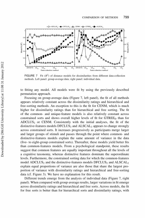
FIGURE 7 Fit (R2) of distance models for dissimilarities from different data-collection
methods. Left panel: group-average data; right panel: individual data.
to fitting any model. All models were fit by using the previously described
permutation approach.
Focusing on group-average data (Figure 7, left panel), the fit of all methods
appears relatively constant across the dissimilarity ratings and hierarchical and
free-sorting methods. An exception to this is the fit for CENM, which is much
higher for dissimilarity ratings than for hierarchical and free sorting. The fit
of the common- and unique-feature models is also relatively constant across
constrained sorts and shows overall higher levels of fit for GTREED than for
ADCLUS2 or CENM. Consistently with the initial analyses, the fit of the
distinctive-features models DFCLUS2 and ALSCAL2 appears to change strongly
across constrained sorts. It increases progressively as participants merge larger
and larger groups of stimuli and passes through the point where common- and
distinctive-features models explain the same amount of variance in the data
(five- to eight-group constrained sorts). Thereafter, these models yield better fits
than common-features models. From a psychological standpoint, these results
suggest that common features are equally important throughout all the levels of
a cognitive taxonomy, whereas distinctive features dominate the superordinate
levels. Furthermore, the constrained sorting data for which the common-features
model ADCLUS2 and the distinctive-features models DFCLUS2 and ALSCAL2
explain equal proportions of variance are also those that share the largest pro-
portion of variance with dissimilarity ratings and hierarchical and free-sorting
data (cf. Figure 3). We have no explanation for this result.
Different trends emerge from the analysis of individual data (Figure 7, right
panel). When compared with group-average results, larger variations in fit emerge
across dissimilarity ratings and hierarchical and free sorts. Across models, the fit
for free sorts is better than for hierarchical sorts and dissimilarity ratings, with
Dow
nloa
ded
by [
McG
ill U
nive
rsity
Lib
rary
] at
11:
08 3
1 Ja
nuar
y 20
12

800 GIORDANO ET AL.
the exception of the unsurprising perfect fit of GTREED for hierarchical sorts.
Three results emerge from the analysis of individual constrained sorts. Firstly,
the unique-features model (CENM) explains a larger proportion of variance
for individual than for group-average data, with fits that progressively decrease
as participants merge larger and larger groups of stimuli. Secondly, the fit of
the common- and distinctive-features models varies across the constrained sorts.
Finally, the fit of all models follows a U-shape function of the number of groups
in the constrained sorting data.
One potential explanation for the difference of results across group-average
and individual data focuses on the violation of the triangle inequality, a metric
axiom according to which the distance between objects A and B is always
equal to or less than the sum of the distances of A and B from a third object.
This metric axiom is implicit in the MDS and DFCLUS models and in all
graph-theoretic models, but not in ADCLUS (Navarro & Lee, 2004; Sattath &
Tversky, 1977; Tversky, 1977). In particular, Ashby, Maddox, and Lee (1994)
showed that the averaging process decreases the number of violations of the
triangle inequality, and improves the fit of MDS models compared with what is
observed for individual data. Consistently with this interpretation, group-average
dissimilarity ratings were characterized by fewer violations than were individual
data (average number of violations D 0.02 and 0.32, respectively). Notably,
this explanation does not account for the results for sorting data because, by
definition, they satisfy the triangle inequality at the group-average and individ-
ual levels. Another explanation for the different results for group-average and
individual data focuses on the distributional properties of the input dissimilarities
and on the sensitivity of the distance models to such variations (Ghose, 1998;
Pruzansky et al., 1982). We thus assessed the extent to which model fit was
influenced by the skewness and elongation (proportion of elongated triangles
in the distance matrix) of the input data. For each of the distance models, we
computed a multiple rank-regression model (Iman & Conover, 1979), with model
fit as dependent variable and skewness and elongation as predictors (Table 3).
We considered group-average and individual data together. To consider the same
number of group-average and individual datapoints, model fit, skewness, and
elongation were averaged across individuals. Within the rank-regression model,
the strength of the effect of the predictors was measured by their partial R2
(R2p) within the multivariate model (Mulaik, 2005), as computed based on the
observed values of model fit rather than on the ranked values.
Overall, data skewness and elongation explained the variations in the fit
of distinctive-features models better than those of common-features models,
with intermediate levels of explained variance for the unique-features model.
Consistently with the results of Pruzansky, Tversky, and Carroll (1982) and
Ghose (1998), the fit of GTREED improved for lower skewness values, whereas
that of all the other models, ALSCAL2 included, improved for higher skewness
Dow
nloa
ded
by [
McG
ill U
nive
rsity
Lib
rary
] at
11:
08 3
1 Ja
nuar
y 20
12
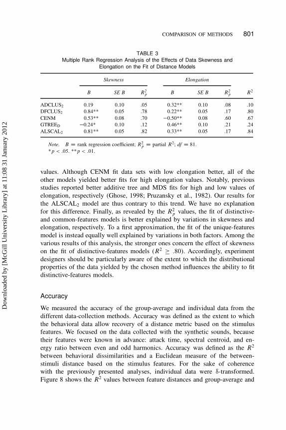
COMPARISON OF METHODS 801
TABLE 3
Multiple Rank Regression Analysis of the Effects of Data Skewness and
Elongation on the Fit of Distance Models
Skewness Elongation
B SE B R2p B SE B R2
p R2
ADCLUS2 0.19 0.10 .05 0.32** 0.10 .08 .10
DFCLUS2 0.84** 0.05 .78 0.22** 0.05 .17 .80
CENM 0.53** 0.08 .70 �0.50** 0.08 .60 .67
GTREED �0.24* 0.10 .12 0.46** 0.10 .21 .24
ALSCAL2 0.81** 0.05 .82 0.33** 0.05 .17 .84
Note. B D rank regression coefficient; R2p D partial R2; df D 81.
*p < :05. **p < :01.
values. Although CENM fit data sets with low elongation better, all of the
other models yielded better fits for high elongation values. Notably, previous
studies reported better additive tree and MDS fits for high and low values of
elongation, respectively (Ghose, 1998; Pruzansky et al., 1982). Our results for
the ALSCAL2 model are thus contrary to this trend. We have no explanation
for this difference. Finally, as revealed by the R2p values, the fit of distinctive-
and common-features models is better explained by variations in skewness and
elongation, respectively. To a first approximation, the fit of the unique-features
model is instead equally well explained by variations in both factors. Among the
various results of this analysis, the stronger ones concern the effect of skewness
on the fit of distinctive-features models (R2 � :80). Accordingly, experiment
designers should be particularly aware of the extent to which the distributional
properties of the data yielded by the chosen method influences the ability to fit
distinctive-features models.
Accuracy
We measured the accuracy of the group-average and individual data from the
different data-collection methods. Accuracy was defined as the extent to which
the behavioral data allow recovery of a distance metric based on the stimulus
features. We focused on the data collected with the synthetic sounds, because
their features were known in advance: attack time, spectral centroid, and en-
ergy ratio between even and odd harmonics. Accuracy was defined as the R2
between behavioral dissimilarities and a Euclidean measure of the between-
stimuli distance based on the stimulus features. For the sake of coherence
with the previously presented analyses, individual data were •-transformed.
Figure 8 shows the R2 values between feature distances and group-average and
Dow
nloa
ded
by [
McG
ill U
nive
rsity
Lib
rary
] at
11:
08 3
1 Ja
nuar
y 20
12

802 GIORDANO ET AL.
FIGURE 8 Accuracy of group-average and individual dissimilarities D R2 between
dissimilarities and Euclidean distance based on known stimulus features. R2 measures are
shown on a logarithmic scale to improve the readability of individual-level results.
individual data. Because of the fact that accuracy was measured with reference
to a Euclidean distance based on the features, between-methods differences in
accuracy might be influenced by the ability to fit a Euclidean structure to the
various behavioral data sets. However, alternative accuracy measures based on
alternative metrics of the feature-based distance (e.g., additive tree) produced
the same results, and are not shown here for the sake of brevity.
Several points emerge from this analysis. First, and not surprisingly, less
noisy group-average data are more accurate than individual data. Second, and
consistently with previous studies, dissimilarity ratings are by far the most
accurate method (Bricker & Pruzansky, 1970; Subkoviak & Roecks, 1976).
Third, free sorting and hierarchical sorting are equally accurate at the group-
average level, whereas hierarchical sorts are more accurate at the individual
level. The first of these results is in contrast with the superior accuracy of group-
average hierarchical sorts compared with free sorts observed by Rao and Katz
(1971). Several methodological differences might explain this inconsistency. For
example, Rao & Katz assumed a Euclidean mental space and measured accuracy
in MDS models fit to the dissimilarities. Our data sets were better fit with graph-
theoretic structures, and the analysis of accuracy focused on the raw data. Among
Dow
nloa
ded
by [
McG
ill U
nive
rsity
Lib
rary
] at
11:
08 3
1 Ja
nuar
y 20
12

COMPARISON OF METHODS 803
the various factors, a particular aspect of the free sorts simulated by Rao and Katz
appeared to provide a straightforward explanation for the divergence. In their
study, the maximum number of free-sorting groups was proportionally lower than
was observed with the participants in our experiment (8 groups/40 stimuli D
0.2 for Rao and Katz; 6.15 groups/20 stimuli D 0.31 in this study). As such,
the free-sorting data from their study are likely more comparable to the four-
group constrained sorts than to the free sorts from the present study (4 groups/20
stimuli D 0.2). Based on these considerations, our results are consistent with
those of Rao and Katz at the group-average and individual levels: in both cases,
the four-group constrained sorts are less accurate than the hierarchical sorts. The
superior accuracy of individual sorts also provides at least partial support for the
hypothesis that hierarchical sorting produces data that are more appropriate than
free-sorting data for individual-differences scaling (Lawless et al., 1995). Indeed,
more accurate individual data are more likely to yield interpretable solutions for
individual-differences models.
CONCLUSIONS
We compared dissimilarity ratings and sorting methods relative to a variety
of factors of potential relevance to the experiment design process: efficiency,
reliability, between-method redundancy, data modeling, and accuracy. Table 4
ranks the various methods relative to most of these criteria.
Consistently with previous studies, dissimilarity ratings scored as a highly
inefficient method for large stimulus sets, whereas free sorting was drastically
more efficient. When compared to dissimilarity ratings, the gain in efficiency
associated with hierarchical sorting appeared to be minimal if participants were
asked to create the entire hierarchy. Interestingly, modeling results showed that
the truncated hierarchical sorting methods are at least as efficient as free sorting.
The analysis of reliability revealed an efficiency–reliability tradeoff: less efficient
TABLE 4
Rank Ordering of Nonderived Data-Collection Methods Relative to
Various Criteria Investigated
Dissimilarity
Ratings
Hierarchical
Sorting
Free
Sorting
Efficiency Low Medium High
Reliability High Medium Low
Accuracy (group) High Medium Medium
Accuracy (indiv.) High Medium Low
Note. Group D group-average data; indiv. D individual data.
Dow
nloa
ded
by [
McG
ill U
nive
rsity
Lib
rary
] at
11:
08 3
1 Ja
nuar
y 20
12

804 GIORDANO ET AL.
methods that required participants to inspect each stimulus a larger number of
times produced more reliable data, more likely to be replicated with different
groups of participants. Dissimilarity ratings and free sorting were thus the most
and least reliable methods, respectively, with an intermediate reliability for
hierarchical sorting. Similar results emerged from the analysis of data accuracy:
dissimilarity ratings reflected the stimulus features more closely than any of the
sorting methods at the group-average and individual levels. The plausible hy-
pothesis of an efficiency–accuracy tradeoff is mitigated by the fact that although
hierarchical sorting was more accurate than free sorting at the individual level,
both methods appeared equally accurate at the group-average level.
The analysis of cross-method redundancy revealed that group-average dissim-
ilarity ratings and hierarchical and free-sorting dissimilarities share a consider-
able amount of variance, approximately 60%. These results might in principle
support the choice of more efficient sorting methods over dissimilarity ratings.
This choice should nonetheless take the lower accuracy and reliability of sorting
methods into account. Because of these latter properties, sorting methods should
be adopted with extreme parsimony and only when strictly necessary (e.g.,
strong adaptation effects; measurement of context effects vulnerable to long
dissimilarity–estimation sessions). The choice of sorting methods should be cau-
tious even when dealing with large sets of stimuli. In such cases, and depending
on the available resources, the experimenter might thus still opt for dissimilarity
ratings and distribute the judgment of the various pairs of stimuli across different-
day experimental sessions, and collect multiple ratings of each of the pairs from
each of the participants. In the absence of the necessary conditions, truncated
hierarchical sorting should be considered as the best alternative to dissimilarity
ratings. Redundancy analyses showed that truncated hierarchical sorts contain
a very large amount of information about the complete hierarchical sorts even
when the starting number of groups is less than one third of the number of exper-
imental stimuli. For this reason, truncated hierarchical sorting is highly likely to
keep the higher individual-level accuracy and reliability of complete hierarchical
sorts while at the same time attaining similar efficiency levels as free sorting.
Overall, the analysis of data-modeling biases revealed that the fit of distinctive-
features models such as MDS is particularly sensitive to a change in data-
collection methods. This effect appears to be strongly dependent on the skew-
ness of the dissimilarities. In particular, and consistently with previous studies,
distinctive-features models better fit data with a moderately negative to positive
skeweness. Given the relatively strong dependence of model fit on the data-
collection method, it is recommended to carry out analyses based on the raw
unmodeled dissimilarities as frequently as possible. In the case of strong interest
for distance models, the experimenter is advised to evaluate the robustness of the
main conclusions against variations in the data-collection method, and against
variations in the distance model itself (e.g., test whether MDS and additive-tree
Dow
nloa
ded
by [
McG
ill U
nive
rsity
Lib
rary
] at
11:
08 3
1 Ja
nuar
y 20
12

COMPARISON OF METHODS 805
models of the same data suggest the perceptual relevance of the same stimulus
features).
ACKNOWLEDGMENTS
Portions of this research were reported at the 50th Annual Meeting of the Psy-
chonomic Society in Boston, Massachusetts, in November 2009. This work was
supported by Stephen McAdams’ Canada Research Chair in Music Perception
and Cognition, by a grant from the Natural Sciences and Engineering Research
Council of Canada to Stephen McAdams (RGPIN 312774-05) and by a Special
Research Opportunity Grant from the Natural Sciences and Engineering Re-
search Council of Canada (NSERC). The authors wish to thank Daniel J. Navarro
for discussions on fitting routines for the MCM model and two anonymous
reviewers and Yoshio Takane for useful suggestions.
REFERENCES
Arabie, P., Carroll, J. D., & DeSarbo, W. (1987). Three-way scaling and clustering. Newbury Park,
CA: Sage.
Ashby, F., Maddox, W., & Lee, W. (1994). On the dangers of averaging across subjects when using
multidimensional scaling or the similarity-choice model. Psychological Science, 5, 144–151.
Barthélemy, J. P., & Guénoche, A. (1991). Trees and proximity representations. Chichester, England:
Wiley.
Bertino, M., & Lawless, H. T. (1993). Understanding mouthfeel attributes: A multidimensional
scaling approach. Journal of Sensory Studies, 8, 101–114.
Bijmolt, T. H. A., & Wedel, M. (1995). The effects of alternative methods of collecting similarity
data for multidimensional scaling. International Journal of Research in Marketing, 12, 363–371.
Bimler, D. L., & Kirkland, J. (1997). Multidimensional scaling of hierarchical sorting data applied
to facial expressions. Scandinavian Journal of Psychology, 38, 349–357.
Bimler, D. L., Kirkland, J., & Chen, S.-J. (1998). A cross-cultural study of facial expressions of
emotion using multidimensional scaling (Annual Report No. 21). Research and Clinical Center
for Child Development, Hokkaido University.
Bonebright, T. L. (1996). An investigation of data collection methods for auditory stimuli: Paired
comparisons versus a computer sorting task. Behavior Research Methods, Instruments, and
Computers, 28, 275–278.
Borg, I., & Groenen, P. (1997). Modern multidimensional scaling. New York, NY: Springer-Verlag.
Boster, J. (1986). Can individuals recapitulate the evolutionary development of color lexicons?
Ethnology, 25, 61–74.
Bricker, P. D., & Pruzansky, S. (1970). Comparison of sorting and pairwise similarity judgment
techniques for scaling auditory stimuli. Journal of the Acoustical Society of America, 47(1A),
96–96.
Caclin, A., McAdams, S., Smith, B. K., & Winsberg, S. (2005). Acoustic correlates of timbre space
dimensions: A confirmatory study using synthetic tones. Journal of the Acoustical Society of
America, 118, 471–482.
Carroll, J. D. (1976). Spatial, non-spatial and hybrid models for scaling. Psychometrika, 41, 439–463.
Dow
nloa
ded
by [
McG
ill U
nive
rsity
Lib
rary
] at
11:
08 3
1 Ja
nuar
y 20
12

806 GIORDANO ET AL.
Carroll, J. D., & Arabie, P. (1983). INDCLUS: An individual differences generalization of the
ADCLUS model and the MAPCLUS algorithm. Psychometrika, 48, 157–169.
Carroll, J. D., & Pruzansky, S. (1980). Discrete and hybrid scaling models. In E. D. Lantermann
& H. Feger (Eds.), Similarity and choice, papers in honour of Clyde Coombs (pp. 108–139).
Bern, Switzerland: Hans Huber.
Cartier, R., Rytz, A., Lecomte, A., Poblete, F., Krystlik, J., Belin, E., et al. (2006). Sorting procedure
as an alternative to quantitative descriptive analysis to obtain a product sensory map. Food
Quality and Preference, 17, 562–571.
Chaturvedi, A., & Carroll, J. D. (2006). CLUSCALE (“CLUstering and multidimensional
SCAL[E]ing”): A three-way hybrid model incorporating overlapping clustering and multidi-
mensional scaling structure. Journal of Classification, 23, 269–299.
Corter, J. E. (1996). Tree models of similarity and association. Thousand Oaks, CA: Sage.
Corter, J. E. (1998). An efficient metric combinatorial algorithm for fitting additive trees. Multivariate
Behavioral Research, 33, 249–271.
Coxon, A. P. M. (1999). Sorting data: Collection and analysis. Thousand Oaks, CA: Sage.
Dragsgow, F., & Jones, L. E. (1979). Multidimensional scaling of derived dissimilarities. Multivariate
Behavioral Research, 14, 227–244.
Efron, B., & Tibishirani, R. J. (1993). An introduction to the bootstrap. New York, NY: Chapman
and Hall.
Gati, I., & Tversky, A. (1982). Representations of qualitative and quantitative dimensions. Journal
of Experimental Psychology: Human Perception and Performance, 8, 325–340.
Ghose, S. (1998). Distance representations of consumer perceptions: Evaluating appropriateness by
using diagnostics. Journal of Marketing Research, 35, 137–153.
Giordano, B. L., McDonnell, J., & McAdams, S. (2010). Hearing living symbols and nonliving
icons: Category-specificities in the cognitive processing of environmental sounds. Brain and
Cognition, 73, 7–19.
Goldstone, R. L. (1994). The role of similarity in categorization: Providing a framework. Cognition,
52, 125–157.
Goldstone, R. L. (1999). Similarity. In R. A. Wilson & F. C. Keil (Eds.), MIT encyclopedia of the
cognitive sciences (pp. 763–764). Cambridge, MA: MIT Press.
Goodhill, G. J., Simmen, M. W., & Willshaw, D. J. (1995). An evaluation of the use of multidi-
mensional scaling for understanding brain connectivity. Philosophical Transactions of the Royal
Society B: Biological Sciences, 348, 265–280.
Graef, J., & Spence, I. (1979). Using distance information in the design of large multidimensional
scaling experiments. Psychological Bulletin, 86, 60–66.
Griffiths, T. L., & Kalish, M. L. (2002). A multidimensional scaling approach to mental multiplica-
tion. Memory and Cognition, 30, 97–106.
Harbke, C. R. (2003). Evaluation of data collection techniques for multidimensional scaling with
large stimulus sets. Unpublished master’s thesis, Washington State University, Department of
Psychology.
Harloff, J., & Coxon, A. P. M. (2005). How to sort: A short guide on sorting investigations. Retrieved
from http://www.methodofsorting.com/HowToSort1-1_English.pdf
Henry, W. A., & Stumpf, R. V. (1975). Time and accuracy measures for alternative multidimensional
scaling data collection methods. Journal of Marketing Research, 12, 165–170.
Holman, E. W. (1972). The relation between hierarchical and euclidean models for psychological
distances. Psychometrika, 37, 417–423.
Hubert, L. J., Arabie, P., & Meulman, J. (1997). Linear and circular unidimensional scaling for
symmetric proximity matrices. British Journal of Mathematical and Statistical Psychology, 50,
253–284.
Hubert, L. J., Arabie, P., & Meulman, J. (2006). The structural representation of proximity matrices
with MATLAB. Philadelphia, PA, and Alexandria, VA: SIAM and ASA.
Dow
nloa
ded
by [
McG
ill U
nive
rsity
Lib
rary
] at
11:
08 3
1 Ja
nuar
y 20
12

COMPARISON OF METHODS 807
Iman, R., & Conover, W. (1979). The use of the rank transform in regression. Technometrics, 21,
499–509.
International Organization for Standardization. (2004). Acoustics – Reference zero for the calibration
of audiometric equipment – Part 8: Reference equivalent threshold sound pressure levels for
pure tones and circumaural earphones (ISO 389–8) (Tech. Rep.). International Organization
for Standardization, Geneva, Switzerland.
Johnson, M. D., Lehmann, D. R., & Horne, D. R. (1990). The effects of fatigue on judgments of
interproduct similarity. International Journal of Research in Marketing, 7, 35–43.
Johnson, S. C. (1967). Hierarchical clustering schemes. Psychometrika, 32, 241–254.
Kendall, D. G. (1975). The recovery of structure from fragmentary information. Philosophical
Transactions for the Royal Society of London. Series A, Mathematical and Physical Sciences,
279, 547–582.
Kroonenberg, P. M. (2008). Applied multiway data analysis. Hoboken, NJ: Wiley.
Lawless, H. T., Sheng, N., & Knoops, S. S. C. P. (1995). Multidimensional scaling of sorting data
applied to cheese perception. Food Quality and Preference, 6, 91–98.
Malhotra, N. K. (1990). Comment on: “The effects of fatigue on judgments of interproduct similar-
ity,” by M. D. Johnson, D. R. Lehmann, and D. R. Horne. International Journal of Research
in Marketing, 7, 45–51.
Martin, F. N., & Champlin, C. A. (2000). Reconsidering the limits of normal hearing. Journal of
the American Academy of Audiology, 11, 64–66.
Miller, G. A. (1956). The magical number seven, plus or minus two: Some limits on our capacity
for processing information. The Psychological Review, 63, 81–97.
Miller, G. A. (1969). A psychological method to investigate verbal concepts. Journal of Mathematical
Psychology, 6, 169–191.
Mulaik, S. (2005). Variable selection. In B. S. Everitt & D. C. Howell (Eds.), Encyclopedia of
statistics in behavioral science (pp. 2107–2110). Chichester, England: Wiley.
Navarro, D. J., & Lee, M. D. (2004). Common and distinctive features in stimulus similarity: A
modified version of the contrast model. Psychonomic Bulletin and Review, 11, 961–974.
Pruzansky, S., Tversky, A., & Carroll, J. D. (1982). Spatial versus tree representations of proximity
data. Psychometrika, 47, 3–24.
Rao, V. R., & Katz, R. (1971). Alternative multidimensional scaling methods for large stimulus sets.
Journal of Marketing Research, 8, 488–494.
Rosenberg, S., & Kim, M. P. (1975). The method of sorting as a data-gathering procedure in
multivariate research. Multivariate Behavioral Research, 10, 489–502.
Sattath, S., & Tversky, A. (1977). Additive similarity trees. Psychometrika, 42, 319–345.
Shepard, R. N. (1962a). The analysis of proximities: Multidimensional scaling with an unknown
distance function. I. Psychometrika, 27, 125–140.
Shepard, R. N. (1962b). The analysis of proximities: Multidimensional scaling with an unknown
distance function. II. Psychometrika, 27, 219–246.
Shepard, R. N. (1987). Toward a universal law of generalization for psychological science. Science,
237, 1317–1323.
Shepard, R. N., & Arabie, P. (1979). Additive clustering: Representation of similarities as combi-
nations of discrete overlapping properties. Psychological Review, 86, 87–123.
Simmen, M. W. (1996). Multidimensional scaling of binary dissimilarities: Direct and derived
approaches. Multivariate Behavioral Research, 31, 47–67.
Spence, I., & Domoney, D. W. (1974). Single subject incomplete designs for nonmetric multidimen-
sional scaling. Psychometrika, 39, 469–490.
Subkoviak, M. J., & Roecks, A. L. (1976). A closer look at the accuracy of alternative data-collection
methods for multidimensional scaling. Journal of Educational Measurement, 13, 309–317.
Takane, Y., Young, F. W., & De Leeuw, J. (1977). Nonmetric individual differences multidimensional
scaling: An alternating least squares method with optimal scaling features. Psychometrika, 42,
7–67.
Dow
nloa
ded
by [
McG
ill U
nive
rsity
Lib
rary
] at
11:
08 3
1 Ja
nuar
y 20
12

808 GIORDANO ET AL.
Torgerson, W. S. (1952). Multidimensional scaling: I. Theory and method. Psychometrika, 17, 401–
419.
Tsogo, L., Masson, M. H., & Bardot, A. (2000). Multidimensional scaling methods for many-object
sets: A review. Multivariate Behavioral Research, 35, 307–319.
Tversky, A. (1977). Features of similarity. Psychological Review, 84, 327–352.
Tversky, A., & Gati, I. (1978). Studies of similarity. In E. Rosch & B. B. Lloyd (Eds.), Cognition
and categorization (pp. 79–98). Mahwah, NJ: Erlbaum.
Ward, L. M. (1977). Multidimensional scaling of the molar physical environment. Multivariate
Behavioral Research, 12, 23–42.
Winsberg, S., & Carroll, J. D. (1989). A quasi–nonmetric method for multidimensional scaling via
an extended Euclidean model. Psychometrika, 54, 217–229.
APPENDIX
Distance Models
Distance models can be classified into three categories: spatial models, set-
theoretic models, and graph-theoretic models (Corter, 1996). All of the con-
sidered models assume that the distance between objects is a function of their
features, which can be of three types: common features, which increase the
similarity of the objects that share them; distinctive features, which increase
the dissimilarity of the objects that do not share them (Tversky, 1977); unique
features, or specificities (Winsberg & Carroll, 1989), a special type of distinctive
feature that characterizes only one of the objects in the set.
The distance models presented here are appropriate for the analysis of two-
way data. Three-way extensions of part of the models presented here were
described in Arabie, Carroll, and DeSarbo (1987), Kroonenberg (2008), and
Carroll and Arabie (1983).
Spatial Models
Spatial models represent the dissimilarity dij between objects i and j , with
i; j D 1; : : : ; N , as their distance d 0ij in a space. In the multidimensional scaling
(MDS) model
d 0ij D
"
DX
dD1
�
xid � xjd
�r
#1=r
(2)
where D is the number of dimensions, xid is the coordinate of object i along
the d th dimension, and r is the power of the Minkowski metric. The classical
MDS model is metric and the space is Euclidean (i.e., d 0ij is a linear function
of dij and r D 2; Torgerson, 1952). In the nonmetric MDS model, d 0ij is
more generally a monotonic function of dij (Shepard, 1962a; Shepard, 1962b).
Dow
nloa
ded
by [
McG
ill U
nive
rsity
Lib
rary
] at
11:
08 3
1 Ja
nuar
y 20
12

COMPARISON OF METHODS 809
Taking into account the translational invariance of MDS models (i.e., the fact that
the configuration can be translated arbitrarily without affecting the distances),
the number of free parameters equals D.N � 1/. MDS can be considered a
distinctive-features model, because features common to all objects (e.g., shape
for triangles of different colors) do not affect their distance (Gati & Tversky,
1982).
Set-Theoretic Models
In this class of models, objects are conceived as collections of features. One of
the most general formulations is the contrast model (Tversky, 1977). In a recent
variant of the contrast model, the modified contrast model (MCM; Navarro &
Lee, 2004), the between-objects proximity s0ij equals
s0ij D c C sc0
ij C sd 0ij
sc0ij D
X
k2CF
wkfikfjk
sd 0ij D �
1
2
X
k2DF
wkfik
�
1 � fjk
�
�1
2
X
k2DF
wkfjk .1 � fik/ (3)
where c is a constant term modeling the saliency of a universal feature common
to all stimuli (Shepard & Arabie, 1979), sc0ij and sd 0
ij are the common- and
distinctive-features proximity metrics, f D .1; : : : ; K/ is a feature that can be
either common (CF ) or distinctive (DF ), and wk is the weight of the kth feature.
The MCM is a hybrid common and distinctive features model. It reduces to
the common-features additive-clustering model (ADCLUS; Shepard & Arabie,
1979) and to the distinctive-features model (DFCLUS; Navarro & Lee, 2004) if
DF D ; or CF D ;, respectively. Present opinions diverge on the number of
free parameters in a set-theoretic model. For ADCLUS, this number equals KC1
(Shepard & Arabie, 1979; see also Navarro & Lee, p. 966), N C K C 1 (Carroll
& Arabie, 1983), and NK C 1 (Chaturvedi & Carroll, 2006). The disagreement
likely extends to DFCLUS and MCM.
Graph-Theoretic Models
Graph-theoretic structures model distances as the minimum-length path between
nodes, each representing an object. A path is a sequence of arcs (e.g., Figure 3).
A particularly important graph-theoretic structure is the tree, that is, a graph
that is connected (each pair of nodes is connected by a path) and does not have
cycles (each path passes through one node only once; Corter, 1996).
Dow
nloa
ded
by [
McG
ill U
nive
rsity
Lib
rary
] at
11:
08 3
1 Ja
nuar
y 20
12

810 GIORDANO ET AL.
In the additive tree (Carroll, 1976; Sattath & Tversky, 1977), distances satisfy
the additive inequality:
dij C dkl � max�
dik C djl ; di l C djk
�
(4)
implying that for each quadruple of objects, the two largest of the three sums
in Equation (4) are equal (Barthélemy & Guénoche, 1991). In a rooted additive
tree, all the paths descend from a common point (e.g., Figure 3). In principle,
an additive tree can be rooted in infinitely many different ways (i.e., the root
can be located on any point in the tree). Commonly, one uses the minimum-
variance root, which minimizes the variance of its distances from all the objects
(Sattath & Tversky, 1977). Under this condition, the root can be thus taken as a
representation of the stereotypical stimulus for the set. An additive-tree model
requires the estimation of 2N � 3 parameters (Sattath & Tversky). Additive
trees can yield both a distinctive-features dissimilarity and a common-features
similarity metric. In the first widely known case, the minimum-path distance
between two objects models the weight of unshared features (Tversky, 1977).
In the second, frequently ignored case, the length of an arc models the weight
of the features common to the object that descend from the same arc (Tversky,
1977). Note that whereas the distinctive-features dissimilarity is independent of
the location of the root, the common-features similarity depends on the location
of the root.
Ultrametric trees, among which the hierarchical clustering model (S. C.
Johnson, 1967), are a special case of the additive tree. In ultrametric trees, objects
are equidistant from the root, and distances satisfy the ultrametric inequality:
dij � max�
dik ; djk
�
(5)
which implies that each possible triad of objects defines an isosceles triangle.
An ultrametric tree is specified by N � 1 parameters. As with additive trees,
ultrametric trees can yield a common-features proximity, the length of an arc
from which two objects descend (Corter, 1996), and a distinctive-features dis-
tance, the minimum-length path between objects. Differently from additive trees,
however, the sum of these two metrics is the same for each pair of objects. As
such, in an ultrametric tree it is not possible to distinguish between common-
and distinctive-features metrics.
An additive tree with a single internal node is called a singular tree, (Sattath &
Tversky, 1977) or star tree or centroid distance (Barthélemy & Guénoche, 1991).
With the centroid distance, the additive inequality reduces to the equality of all
of the three sums in Equation (4) (Corter, 1996), and distances are modeled as
d 0ij D xi C xj (6)
Dow
nloa
ded
by [
McG
ill U
nive
rsity
Lib
rary
] at
11:
08 3
1 Ja
nuar
y 20
12

COMPARISON OF METHODS 811
The least-squares estimation of the x terms is given by
xi D
NP
j D1;j ¤i
dij C k
N � 2�
NP
iD1
NP
j D1;j ¤i
dij C k
2 .N � 1/ .N � 2/(7)
where k is a constant term appropriately chosen to ensure positivity of xi ;
with i D 1; : : : ; N (Hubert, Arabie, & Meulman, 1997). A centroid distance
estimates N parameters. A formulation of the centroid distance similar to that
in Equation (6) is used in EXSCAL, a hybrid of a tree and an MDS model
(Winsberg & Carroll, 1989). When the spatial component is null, EXSCAL
reduces to
d 0ij D
�
xi C xj
�1=2(8)
where the x terms, termed specificities, weight the attributes specific to each
of the stimuli. Independent of the particular formulation, the centroid distance
can be interpreted as a unique-features model. Overall, these models can be
interpreted as a measure of the weight of features unique to each of the objects.
Note finally that an additive tree can always be decomposed in infinitely
many ways as the sum of an ultrametric tree and a centroid metric (Barthélemy
& Guénoche, 1991). The ambiguity of the decomposition reflects the fact that
an additive tree can be rooted in infinitely many ways. As such, an additive
tree can also be interpreted as the sum of a unique-features dissimilarity with
an ultrametric tree, which might be equally well interpreted as a model of
distinctive-features dissimilarity or of common-features similarity.
Dow
nloa
ded
by [
McG
ill U
nive
rsity
Lib
rary
] at
11:
08 3
1 Ja
nuar
y 20
12
Related Documents