Comparison of methods for analysing salmon habitat rehabilitation designs for regulated rivers

RIVER RESEARCH AND APPLICATIONS

River. Res. Applic. 25: 745–772 (2009)

Published online 18 August 2008 in Wiley InterScience

COMPARISON OF METHODS FOR ANALYSING SALMON HABITATREHABILITATION DESIGNS FOR REGULATED RIVERS

ROCKO A. BROWN and GREGORY B. PASTERNACK*

Department of Land, Air and Water Resources, University of California, One Shields Avenue, CA 95616, USA

(www.interscience.wiley.com) DOI: 10.1002/rra.1189

ABSTRACT

River restoration practices aiming to sustain wild salmonid populations have received considerable attention in the Unites Statesand abroad, as cumulative anthropogenic impacts have caused fish population declines. An accurate representation of local depthand velocity in designs of spatially complex riffle-pool units is paramount for evaluating such practices, because these twovariables constitute key instream habitat requirements and they can be used to predict channel stability. In this study, threemodels for predicting channel hydraulics—1D analytical, 1D numerical and 2D numerical—were compared for two theoreticalspawning habitat rehabilitation (SHR) designs at two discharges to constrain the utility of these models for use in riverrestoration design evaluation. Hydraulic predictions from each method were used in the same physical habitat quality andsediment transport regime equations to determine how deviations propagated through those highly nonlinear functions toinfluence site assessments. The results showed that riffle-pool hydraulics, sediment transport regime and physical habitat qualitywere very poorly estimated using the 1D analytical method. The 1D and 2D numerical models did capture characteristiclongitudinal profiles in cross-sectionally averaged variables. The deviation of both 1D approaches from the spatially distributed2D model was found to be greatest at the low discharge for an oblique riffle crest with converging cross-stream flow vectors. Asdecision making for river rehabilitation is dependent on methods used to evaluate designs, this analysis provides managers withan awareness of the limitations used in developing designs and recommendations using the tested methods. Copyright# 2008John Wiley & Sons, Ltd.

key words: river restoration; river modelling; river hydraulics; gravel-bed rivers; physical habitat quality; sediment transport regime

Received 28 February 2008; Revised 23 June 2008; Accepted 24 June 2008

INTRODUCTION

Spawning habitat rehabilitation (SHR) is widely performed for regulated rivers in the western United States and

other semi-arid regions globally (Zeh and Donni, 1994; Wheaton et al., 2004a; Gard, 2006; Elkins et al., 2007) to

mitigate the decline in anadromous fish populations associated with dam impacts and excessive fishing (Yoshiyama

et al., 1998; Graf, 2001). A component of SHR involves adding washed gravel and cobble, 8–256mm in diameter,

to a stream (aka gravel augmentation) to increase the quantity and quality of spawning habitat at a placement site

(Harper et al., 1998; Wheaton et al., 2004a) as well as to provide coarse sediment to transport downstream where it

may form diverse habitats (Trush et al., 2000). In past decades, the design and construction of instream alluvial

spawning habitat using augmented gravels largely involved creating flat homogenous spawning beds supported by

rock weirs (Kondolf et al., 1996; Newbury et al., 1997; Slaney and Zaldokas, 1997; CDFG, 1998; CDWR, 2000;

Saldi-Caromile et al., 2004; Walker et al., 2004). Moreover, the analysis and evaluation of these features also relies

on the assumption of steady, uniform flow to estimate hydraulic variables used in subsequent geomorphic and

ecological predictions.

Based on observed deficiencies of past projects, there is a growing recognition of the importance of design and

implementation of complex alluvial features that utilize channel non-uniformity to promote habitat heterogeneity

(Pasternack et al., 2004; Wheaton et al., 2004b,c; Elkins et al., 2007; Sawyer et al., 2008). There is also a growing

need for accurate and cost-effective means to represent habitat (Maddock, 1999; Moir and Pasternack, 2008).

Consequently, this study presents a comparison of three contemporary analytical and numerical methods used for

*Correspondence to: Gregory B. Pasternack, Department of Land, Air and Water Resources, University of California, One Shields Avenue,Davis, CA 95616, USA. E-mail: [email protected]

Copyright # 2008 John Wiley & Sons, Ltd.

746 R. A. BROWN AND G. B. PASTERNACK

predicting channel hydraulics, spawning habitat quality and sediment transport regime (as defined by ranges in

dimensionless Shields stress; see Methods Section) over riffles and pools typical of regulated rivers where salmon

spawn.

The overall goal of this study was to determine what quantitative differences arise from the three different

approaches for estimating channel hydraulics over riffle and pool sections and to what extent, if any, the differences

impact physical habitat quality and sediment transport predictions. Specific questions were: (1) how do velocity and

water surface profiles compare between each approach for two different discharges and two different riffle-pool

morphologies—one with orthogonal and one with oblique gravel bars? (2) What are the effects of 1D and 2D

hydraulic models on the prediction of sediment transport regime and spawning habitat quality? (3) Can the

hydraulics of even a spatially uniform broad flat riffle (BFR) be determined within reason using only a 1D analytical

approach? (4) How does a blanket-fill gravel placement design differ in sediment transport regime and physical

habitat quality from one that strongly accentuates riffle-pool relief? And (5) what would be the implications of each

approach on decision making for the test designs? The significance of this study lies in the practical aid it provides

regulated-river managers in deciding what level of detail they need in their design evaluation framework to

reasonably predict the outcome of their habitat rehabilitation projects in terms of ecological success and

geomorphic stability.

Riffle-pool units

Riffles and pools are respectively defined as topographic highs and lows along a channel thalweg (Leopold et al.,

1964; Richards, 1976;Wohl et al., 1993). They are a common geomorphic unit for the aquatic community in gravel-

bed rivers with slopes ranging from 0.001 to 0.02, and are thus very important components in SHR projects

involving direct gravel augmentation (NRC, 1992; Newbury et al., 1997; Kondolf, 2000; Saldi-Caromile et al.,

2004; Wheaton et al., 2004a,b; Elkins et al., 2007). Naturally sustained riffles and pools are used by anadromous

fish species through multiple life stages (Bjornn and Reiser, 1991) and represent contrasting hydraulic and

geomorphic environments as indicated by variations in water surface and energy gradients (Leopold et al., 1964;

Keller, 1971; Richards, 1976; Wohl et al., 1993), mean and local bed hydraulic parameters such as velocity and

shear stress (Keller, 1971; Lisle, 1979; Milne, 1982; Carling, 1990; Clifford and Richard, 1992; MacWilliams et al.,

2006), grain size (Keller, 1971) and channel area, which lead to further variations in flow divergence and

convergence (Thompson et al., 1999;MacWilliams et al., 2006).Water-surface and energy gradients over riffles are

typically steeper than over pools at low flows and generally converge as stage increases and relative roughness

decreases (Leopold et al., 1964; Keller, 1971; Richards, 1976; Wohl et al., 1993). Similarly, mean velocity and

shear stress are greater over riffles than pools at lows flows, but the reverse may occur at high flows where channel

conditions promote that phenomenon (Keller, 1971; Carling, 1991; Clifford and Richard, 1992; Wilkinson et al.,

2004; MacWilliams et al., 2006; Harrison and Keller, 2007). Variations in depth, velocity and water surface

gradients between riffles and pools at low flows lead to distinct sediment sorting patterns that may even persist at

high flows and affect channel hydraulics (Keller, 1971; Lisle, 1979). The convergence and/or ‘reversal’ of riffle-

pool water surface elevation (WSE) and velocity profiles can also cause sediment transport capacity to become

greater through pools than riffles (Sear, 1996).

The contrasting hydraulic and geomorphic environments provided by riffle and pool units also yield a nested

hierarchy in the ecological community. In the context of SHR, spawning habitat, defined as suitable areas for

salmon to deposit eggs and for those eggs to incubate, is typically associated with riffle areas, while adult holding

habitat is typically located in pools (Hunter, 1991; Wheaton et al., 2004b; Gard, 2006; Brown and Pasternack,

2008). The linkage between channel hydraulics and what organisms do is often through what is termed ‘physical

habitat’. Physical habitat quality refers to the degree of suitability of local depth, velocity and river-bed substrate

size in a stream to support a particular ecological function. It is a common metric used to evaluate existing channel

conditions for instream flow needs (Smith, 1973; Milhous et al., 1989; Bovee et al., 1998; Lacey and Millar, 2004;

Brown and Pasternack, 2008) as well as in design evaluation for SHR projects (Pasternack et al., 2004; Gard, 2006;

Elkins et al., 2007). Although other variables such as temperature, primary and secondary productivity and water

quality affect the location where fish choose to spend time during a given lifestage (Torgersen et al., 1999; Merz and

Copyright # 2008 John Wiley & Sons, Ltd. River. Res. Applic. 25: 745–772 (2009)

DOI: 10.1002/rra

COMPARING TOOLS FOR RIVER REHABILITATION 747

Setka, 2004), it has been shown that physical habitat quality is often a very strong predictor of some lifestages,

especially spawning (Leclerc et al., 1995; Elkins et al., 2007).

Predicting channel stability and physical habitat quality are important components of evaluating SHR project

designs. The manipulation of channel form that is typical of SHR is related to these key goals through channel

hydraulics, which can be represented at different spatial scales. Engineering and design aspects of direct gravel

augmentation for SHR often require that target depths and velocities are present and that gravels are stable at low

discharges when spawning and embryo incubation are occurring (Merz et al., 2004). In contrast, channel change

and bed turn-over are desired at other times of the year, because the gravel bed needs to be kept free of silt and fine

sand that can cause subsurface oxygen deficits and embryo death (Merz and Setka, 2004; Merz et al., 2004, 2006).

This requirement of bed turnover has stimulated research into design of ‘flushing flows’ that partially mobile the

bed (Wilcock et al., 1996a). Gravel stability and bed-material transport are both related to channel conditions

through shear stress, which is a direct function of channel hydraulics (Yalin, 1977; Chang, 1998). As physical

habitat is also directly linked to channel hydraulics, capturing and distinguishing the hydraulic attributes of riffles

and pools is a key need in the successful design and evaluation for SHR projects (Ghanem et al., 1996).

METHODS

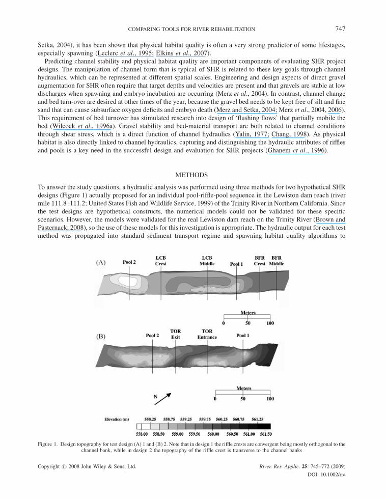
To answer the study questions, a hydraulic analysis was performed using three methods for two hypothetical SHR

designs (Figure 1) actually proposed for an individual pool-riffle-pool sequence in the Lewiston dam reach (river

mile 111.8–111.2; United States Fish andWildlife Service, 1999) of the Trinity River in Northern California. Since

the test designs are hypothetical constructs, the numerical models could not be validated for these specific

scenarios. However, the models were validated for the real Lewiston dam reach on the Trinity River (Brown and

Pasternack, 2008), so the use of these models for this investigation is appropriate. The hydraulic output for each test

method was propagated into standard sediment transport regime and spawning habitat quality algorithms to

Figure 1. Design topography for test design (A) 1 and (B) 2. Note that in design 1 the riffle crests are convergent being mostly orthogonal to thechannel bank, while in design 2 the topography of the riffle crest is transverse to the channel banks

Copyright # 2008 John Wiley & Sons, Ltd. River. Res. Applic. 25: 745–772 (2009)

DOI: 10.1002/rra

748 R. A. BROWN AND G. B. PASTERNACK

evaluate the sensitivity of these metrics to choice of hydraulic estimation method. The sediment transport regime

was characterized by ranges of Shields stress reported in the literature to produce various transport intensities in

gravel-bed rivers. Spawning habitat quality was characterized using a global habitat suitability index based on

depth and velocity. Both of these indices are described in more detail below. Although a specific river was used to

obtain a baseline topography and flow regime, the results should be applicable to channels worldwide with similar

non-dimensional geometric and Froude number scaling.

The comparison of three hydraulic estimation methods required establishing some values for variables and

parameters common to all three methods. To account for the flow dependence of sediment transport regime and

physical habitat quality, the three methods were evaluated at two discharges—the prescribed spawning and embryo

incubation discharge for the Trinity River (8.5m3/s), and the maximum flow release that occurred during 1999–

2004 (170m3/s). For all calculations of design bed material, theD50 (i.e. median size) andD90 (i.e. size that 90% of

grains are smaller than) were assumed to be 76.2 and 152.4mm respectively, based on consultant-recommended

grain sizes for gravel placed into the Trinity River (McBain and Trush, 2003). Similarly, for all parameterizations of

channel roughness, Manning’s nwas used and set at 0.043, which is typical of the channel roughness of well-mixed,

double-washed placed gravels (Pasternack et al., 2004). This value has been validated for use on the Trinity River in

the rehabilitation reach at Lewiston dam over the range of flows evaluated (Brown and Pasternack, 2008). Effects of

channel curvature were not evaluated in this study of straight-channel mechanics, but would be important to

consider for designs of meandering channels.

Test designs

Each test design was situated within the LHR giving the test scenarios several physical constraints. The average

channel width is 35m at low-flow (8.5m3/s and the reach is approximately 600m long with a slope of 0.0022 under

current conditions. However, for this study, the test scenarios were only for the upper 350m of the reach. For more

information on the LHR the reader is referred to Brown and Pasternack (2008).

The morphological features of design 1 (Figure 1(A)) involved a ‘blanket-fill’ of gravel with all areas receiving a

moderate amount of material. The riffle crests were oriented orthogonal to the channel and included a BFR, an ‘L-

shaped’ central bar (LCB), and two constricted pools (hereafter referred to as Pool 1 and Pool 2). The BFR is a

commonly used SHR structure when design is based on 1D methods (Kondolf et al., 1996; CDFG, 1998; CDWR,

2000; Saldi-Caromile et al., 2004). The LCB is an analogue to the central bar, an alluvial morphology that has been

found to provide habitat for multiple life stages of salmonids (Wheaton et al., 2004b). The middle of the LCB has

an asymmetrical cross section where there is a deeper chute on the river left. Constricted pools were used

downstream of the BFR and the LCB to potentially invoke hydraulic reversal and channel self-stability by nature of

the riffles being somewhat wider than pools (Carling, 1990; MacWilliams et al., 2006).

Design 2 (Figure 1(B)) involved placing gravel everywhere, but strongly accentuating the relief between the

main riffle crest and the pools around it. The primary feature was a transverse oblique riffle (TOR) crest in between

two pools. The crest in this case was narrow and attached to an alternate-type bar on river right. This type of bar has

been seen in both natural and artificial riffles. It is similar in function to chevron-shaped riffles, but converges flow

along one bank preferentially, which may enhance local scour there, promoting habitat heterogeneity.

Digital terrain models (DTMs) of both designs were based on the actual channel topography of the Lewiston dam

reach, which was mapped in August 2003 with a resolution of �1.4 points per m2 (Brown and Pasternack, 2008).

For this study, that real surface was re-contoured in AutoCAD Land Desktop 3 to obtain the desired channel

features for each design. The design DTMs (Figure 1) were used to generate the topographic inputs for each test

method.

Hydraulic prediction

Hydraulic variables in regulated rivers serve as key metrics for a plethora of management issues from habitat

assessment, sediment management issues and flood control. In the realm of professional practice and applied

science they aid decision making by facilitating the prediction of other key parameters of interest to the

management of regulated rivers. Since hydraulic variables such as depth and velocity are now widely used as

intermediate links connecting flow processes (i.e. sediment transport and deposition) with ecological conditions in

Copyright # 2008 John Wiley & Sons, Ltd. River. Res. Applic. 25: 745–772 (2009)

DOI: 10.1002/rra

COMPARING TOOLS FOR RIVER REHABILITATION 749

habitat evaluation (Bovee et al., 1998; Maddock, 1999; Gard, 2006; Elkins et al., 2007), as well as geomorphic

processes associated with sediment transport and deposition, their accuracy is vital in attempts to manage and

restore regulated rivers (Pasternack et al., 2006). Currently in professional practice there are three main approaches

for predicting channel hydraulics that can be delineated by the solution procedure and the physical dimensions they

are capable of predicting, and they include a 1D analytical procedure, a 1D numerical model and a 2D numerical

model.

One-dimensional analytical. The 1D analytical method involves predicting open channel processes by coupling

some combination of a mass-conservation equation, empirical hydraulic-geometry equations, empirical flow-

resistance equation and an empirical or semi-empirical sediment-transport equation (Dunne and Leopold, 1978;

Yen, 1991; Rosgen, 1996; Chang, 1998). Flow resistance equations have been typically derived from non-alluvial

channel boundaries under steady, uniform flow and use roughness coefficients that have no true theoretical basis

(Yen, 1991). Because they assume steady, uniform flow conditions, they are the easiest to perform and represent the

lowest cost approach to quantitative design evaluation (Shields et al., 2003).

The Manning–Gauckler equation, hereafter referred to as the Manning equation, is a frequently prescribed flow

resistance equation used in the United States for evaluating channel hydraulics for physical habitat and sediment

transport (Rosgen, 1996; Bovee et al., 1998; Saldi-Caromile et al., 2004), so it was used in this study to calculate

cross-sectionally averaged velocity (V) for each specified WSE:

V ¼ 1

n

� �R2=3S1=2 (1)

and

Q ¼ AV (2)

where Q is the discharge (m3/s), R the hydraulic radius (m), A the cross-sectional area (m2), n the Manning’s

roughness coefficient and S is typically the average bed slope. R and the corresponding Awere obtained iteratively

in AutoCAD Land Desktop 3 until the continuity equation was solved for the discharge of interest. The equation is

very sensitive to S, and the local slope can vary considerably in a gravel-bed river, depending on the spatial scale

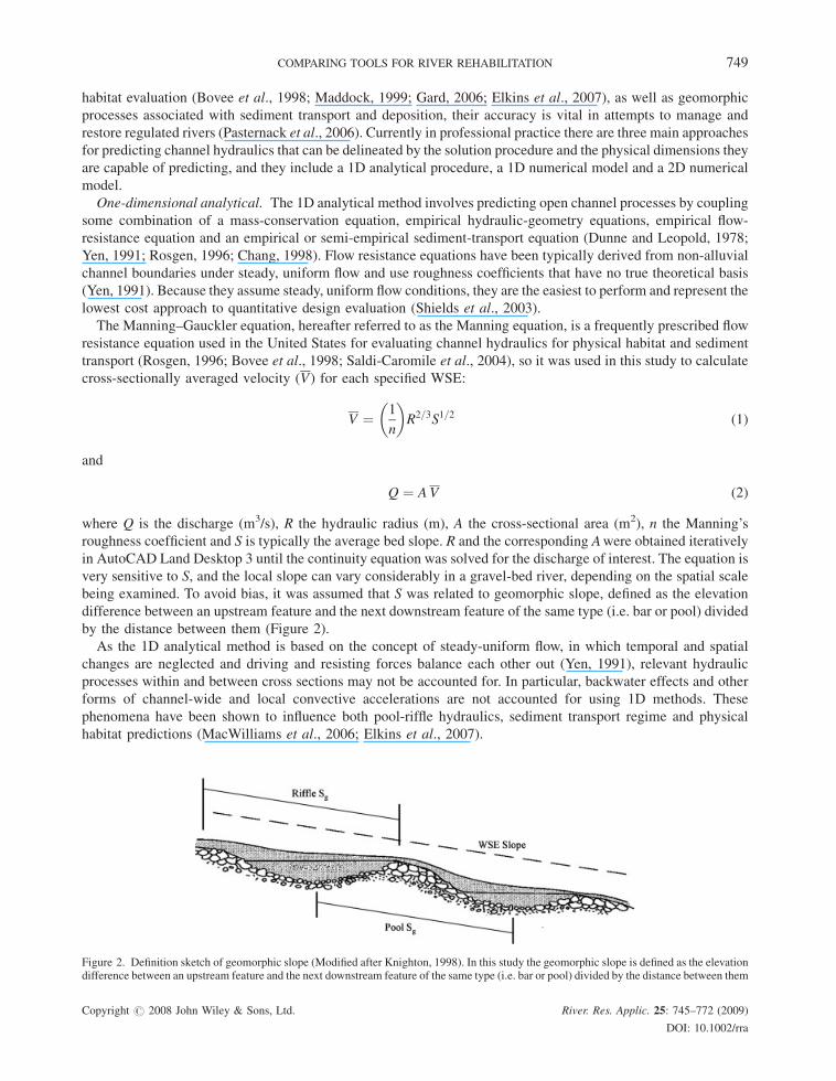
being examined. To avoid bias, it was assumed that S was related to geomorphic slope, defined as the elevation

difference between an upstream feature and the next downstream feature of the same type (i.e. bar or pool) divided

by the distance between them (Figure 2).

As the 1D analytical method is based on the concept of steady-uniform flow, in which temporal and spatial

changes are neglected and driving and resisting forces balance each other out (Yen, 1991), relevant hydraulic

processes within and between cross sections may not be accounted for. In particular, backwater effects and other

forms of channel-wide and local convective accelerations are not accounted for using 1D methods. These

phenomena have been shown to influence both pool-riffle hydraulics, sediment transport regime and physical

habitat predictions (MacWilliams et al., 2006; Elkins et al., 2007).

Figure 2. Definition sketch of geomorphic slope (Modified after Knighton, 1998). In this study the geomorphic slope is defined as the elevationdifference between an upstream feature and the next downstream feature of the same type (i.e. bar or pool) divided by the distance between them

Copyright # 2008 John Wiley & Sons, Ltd. River. Res. Applic. 25: 745–772 (2009)

DOI: 10.1002/rra

750 R. A. BROWN AND G. B. PASTERNACK

One-dimensional numerical model. Numerical approaches to hydraulic estimation employ computers to

approximate solutions of 1D, 2D or 3D equations of motion where the solution procedures are dependant either on

adjacent nodes or cross sections. One-dimensional models such as HEC-RAS and MIKE11 can consider unsteady

conditions and to some extent non-uniform conditions. They cannot account for transitional dynamics where no

cross sections are measured, nor can they account for secondary flow processes that may occur at measured cross

sections (Darby and Van de Wiel, 2003; Nelson et al., 2003). They use a standard step method to iteratively solve

the energy equation from one cross section to the next to calculate water surface profiles. These models solve the

energy equation for steady gradually varied flow and are also capable of calculating subcritical, super critical and

mixed flow regime water surface profiles (Brunner, 1998). The energy equation at two cross sections denoted by

subscript numbers 1 and 2 is described as:

H2 þ Z2 þ a2 V2

2g¼ H1 þ Z1 þ a1 V1

2gþ he (3)

where H is cross-sectionally averaged water depth (m), Z the invert elevation (m), a the velocity weighting

coefficient, g gravitational acceleration (m/s2) and he is energy head loss (m). Equation (1) is used implicitly in the

solution of Equation (3).

HEC-RAS was used in this study and the boundary conditions required to run it were the discharge entering the

upstream boundary, the associated downstream WSE and channel topography at designated cross sections. Cross

sections were sampled from the DTM of each test design in 7.6-m increments. Some additional cross sections were

augmented to capture transitional dynamics and to match cross-section locations used for the 1D analytical method.

One-dimensional hydraulic models usually provide fairly accurate predictions of WSE for flood stages where

relative roughness is low and/or there are gradual changes in bed slope and channel width (Lacey and Millar, 2004;

Ghanem et al., 1996; Brunner, 1998). They have the advantage over 1D analytical approaches in that they can

account for cross-sectionally averaged convergence and divergence effects at cross sections. They cannot account

for topographic variability between cross sections nor even localized convective accelerations within only a small

part of a cross section, such as in the vicinity of a boulder cluster. Previous studies highlight that these models may

not be appropriate for predicting channel hydraulics at the spatial scales necessary to represent physical habitat and

sediment transport (Lacey and Millar, 2004; Ghanem et al., 1996; MacWilliams et al., 2006). Despite this, they are

readily available, require relatively sparse information and are frequently used by professional consultants.

Two-dimensional numerical model. Two-dimensional (depth-averaged) models such as finite element surface

water modelling system 3.1.5 (FESWMS), RIVER2D, HIVEL2D, RMA2, MIKE21, SRH-2D, TUFLOW and

TELEMAC further add the ability to consider full lateral and longitudinal variability down to the sub-meter scale,

including effects of alternate bars, transverse bars, islands and boulder complexes, but require highly detailed

topographic maps of channels and floodplains (French and Clifford, 2000). Two-dimensional models are also more

realistically linked to flow, sediment transport and biological variables measured in the field at the same spatial

scale (Lacey and Millar, 2004; Ghanem et al., 1996; Pasternack et al., 2006). Two-dimensional models have been

used to study a variety of hydrogeomorphic processes (Bates et al. 1992; Leclerc et al., 1995; Miller and Cluer,

1998; Cao et al., 2003). Recently, they have been evaluated for use in regulated river rehabilitation emphasizing

SHR by gravel placement (Pasternack et al., 2004, 2006; Wheaton et al., 2004b; Elkins et al., 2007; Brown and

Pasternack, 2008).

In this study, the 2D model known as FESWMS was used to simulate hydraulics (Froehlich, 1989). FESWMS

solves the vertically integrated conservation of momentum and mass equations using a finite element method to

acquire depth-averaged 2D velocity vectors and water depths at each node in a finite element mesh. The model is

capable of simulating both steady and unsteady 2D flow as well as subcritical and supercritical flows. The basic

governing equations for vertically integrated momentum in the x- and y-directions under the hydrostatic assumption

are given by

@

@tðHUÞ þ @

@xðbuuHUUÞ þ @

@yðbuvHUVÞ þ gH

@zb

@xþ 1

2g þ @H2

@xþ 1

rtbx � @

@xðHtxxÞ � @

@yðHtxyÞ

� �¼ 0 (4a)

Copyright # 2008 John Wiley & Sons, Ltd. River. Res. Applic. 25: 745–772 (2009)

DOI: 10.1002/rra

COMPARING TOOLS FOR RIVER REHABILITATION 751

and

@

@tðHVÞ þ @

@xðbvuHVUÞ þ @

@yðbvvHVVÞ þ gH

@zb

@yþ 1

2gþ @H2

@yþ 1

rtby � @

@xðHtyxÞ � @

@yðHtyyÞ

� �¼ 0 (4b)

where H is local water depth (m), U and Vare local depth-averaged velocity components (m/s) in the horizontal x-

and y-directions, respectively, zb the bed elevation (m), buu, buv, bvu and bvv are the momentum correction

coefficients that account for the variation of velocity in the vertical direction, tax and tbx are the bottom shear

stress components (Pa) acting in the x- and y-directions, respectively, and txx, txy, tyx and tyy are the shear stress

components (Pa) caused by fluid turbulence. Conservation of mass in two dimensions is given by

@H

@tþ @

@xðHUÞ þ @

@yðHVÞ ¼ 0 (5)

FESWMS was implemented using surface water modelling system v. 8.1 graphical user interface (EMS-I, South

Jordan, UT). The boundary conditions required to run FESWMS were the input hydrograph, the exit WSE and high-

resolution channel topography. In addition, model parameters are needed to describe channel roughness and provide

turbulence closure. Values for all boundary conditions and parameters were selected to be physically realistic and

were not numerically calibrated. The turbulence parameter eddy viscosity (E) was a variable in the system of model

equations, and it was computed as E¼ c0 + 0.6Hu�, where u� is shear velocity (m/s) and c0 a minimal constant added

for numerical stability. This equation was implemented in FESWMS to allow eddy viscosity to vary throughout the

channel, which yields more accurate transverse velocity gradients. However, a comparison of 2D and 3Dmodels for a

shallow gravel-bed river demonstrated that even with this spatial variation, it is not enough to yield as rapid lateral

variations in velocity as occurs in natural channels, presenting a fundamental limitation of 2D models like FESWMS

(MacWilliams et al., 2006). Although eddy viscosity is an oversimplifying turbulence closure parameter, observations

of depth and velocity may be used to compute values for it as a check on model performance (Fischer et al., 1979).

This model has previously been heavily validated for use in shallow gravel-bed rivers (Pasternack et al., 2004, 2006;

Wheaton et al., 2004b; Elkins et al., 2007; Brown and Pasternack, 2008; Moir and Pasternack, 2008).

DEM {x,y,z} contour and grid points for each test design were imported fromAutoCAD into the 2Dmodel where

they were used to interpolate the elevations of the nodes in a finite element mesh consisting of triangular and

quadrangular elements. Inter-nodal spacing ranged from 0.2 to 0.6m. To reduce model instability associated with

mesh-element wetting and drying at a threshold of 9-cm depth, meshes were iteratively trimmed to exclude dry

areas, yielding slightly different final meshes for each discharge simulation.

Three-dimensional models such as UNTRIM and SSIIM go further by including vertical fluid fluxes, but do not

require much more data input than 2D models to get going (MacWilliams et al., 2006). However, model validation

of 3D processes is difficult and time consuming. Also, few ecological and geomorphic processes have been

quantitatively linked to 3D flow dynamics yet, limiting the interpretation of 3D model output for practical

applications, such as SHR design. Consequently, 3D models are not considered in this study.

There are obvious discrepancies between analytical calculations versus 1D and 2D hydraulic models (Cao and

Carling, 2002), however, the effect of these differences on sediment transport regime and physical habitat

predictions for riffle and pool units have not been explored. Some previous studies have shown that 1D numerical

models are insufficient to describe hydraulics and sediment transport through pool-riffle sequences (Keller and

Florsheim, 1993; Rathburn and Wohl, 2003). Moreover, studies have shown that 2D models provide a better

description of channel hydraulics and physical habitat than 1D models (Ghanem et al., 1996; Lacey and Millar,

2004; MacWilliams et al., 2006). Such efforts provide a foundation for a thorough investigation of the trade-offs

when using models for river-rehabilitation design evaluation.

Sediment transport regime predictions

In both analytical and numerical approaches Shields stress was used as the representative variable that indicates

channel stability via a sediment transport regime, defined below. For purposes of comparison Shields stress was

calculated as a section average for 1D analytical and numerical approaches and on a node basis for the 2D

Copyright # 2008 John Wiley & Sons, Ltd. River. Res. Applic. 25: 745–772 (2009)

DOI: 10.1002/rra

752 R. A. BROWN AND G. B. PASTERNACK

numerical approach. Shields stress is defined as:

t� ¼ tb

ðgs � g f ÞD50

(6)

where, t� is Shields stress, tb the predicted bed shear stress (Pa), gs the specific weight of sediment (N/m3), g f specific

weight of water (N/m3) and D50 is the median grain size of the bed surface (m). The sediment transport regime was

characterized by the range of values that t� falls into, as defined by Lisle et al. (2000): Values of 0.00< t�< 0.01

mean no transport is occurring, 0.01< t�< 0.03 indicates intermittent, localized transport in response to infrequent

turbulent bursts and/or bed vibrations, 0.03< t�< 0.06 corresponds with Wilcock’s (1996b) domain of ‘partial

transport’ in which grains move in proportion to their relative exposure on the bed surface, and t�> 0.1 represents

full mobility of a ‘carpet’ of sediment 1–2D90 thick. Higher thresholds for channel-altering conditions may exist, but

have not been delineated in the literature. These threshold delineations may vary depending on how well compacted

the bed is and other factors, but they provide a reasonable basis for characterizing sediment transport conditions. At

present there is disagreement as to the breadth of applicability of these dimensionless ranges across all types of

gravel- and sand-bed rivers. However, a review of sediment transport studies in gravel-bed rivers with the

characteristics of the LHR found that they are applicable for the purposes of this study.

To obtain t�, predictions of tb were made using the hydraulic predictions from each method in the same

Einstein’s log-velocity equation for turbulent flows over rough beds

tb ¼ rw u

�5:75 log

12:2H

2D90

� �� �� �2

(7)

where u is depth-average velocity (m/s), D90¼ grain size in which 90% are finer than (m). When used with the 1D

analytical method, V and R are substituted for u and H, respectively. With the 1D numerical method, V and H are

substituted for u and H, respectively. With the 2D numerical method, u is taken to be the magnitude of the velocity

vector at a point.

Physical habitat predictions

A global habitat suitability index (GHSI) for Chinook salmon spawning habitat quality was calculated using

depth (DHSI) and velocity (VHSI) habitat suitability curves that were previously derived for the Trinity River based

on field observations of flow conditions at spawning sites (USFWS, 1997). These curves are typical across rivers in

California. The best fit numerical equations using H or H to match reported DHSI were

For H< 0 and H> 1.374m:

DHSI ¼ 0 (8a)

For 0<H< 1.374m:

DHSI ¼ 0:0351 � 0:7248ðH=0:3048Þ þ 4:9307ðH=0:3048Þ2 � 5:2964ðH=0:3048Þ3

þ 2:4818ðH=0:3048Þ4 � 0:6007ðH=0:3048Þ5 þ 0:007235ðH=0:3048Þ6

� 0:002514ðH=0:3048Þ7 � 0:000274ðH=0:3048Þ8 þ 2:1277ðH=0:3048Þ9 (8b)

Similarly, using either U or V those for VHSI were

For U< 0.01 and U> 1.68m/s:

VHSI ¼ 0 (9a)

For 0.01<U< 0.40m/s:

VHSI ¼ �0:0131 þ 0:5523ðU=0:3048Þ � 0:8246ðU=0:3048Þ2 þ 1:8208ðU=0:3048Þ3

� 0:8013ðU=0:3048Þ4 (9b)

Copyright # 2008 John Wiley & Sons, Ltd. River. Res. Applic. 25: 745–772 (2009)

DOI: 10.1002/rra

COMPARING TOOLS FOR RIVER REHABILITATION 753

For 0.40<U< 1.68m/s:

VHSI ¼ �5:1205 þ 13:1440ðU=0:3048Þ � 9:5769ðU=0:3048Þ2 þ 2:2576ðU=0:3048Þ3

þ 0:4525ðU=0:3048Þ4 � 0:3746ðU=0:3048Þ5 þ 0:08619ðU=0:3048Þ6

� 0:009046ðU=0:3048Þ7 þ 0:000369ðU=0:3048Þ8 (9c)

Similar analyses were done for steelhead and coho as well as for all three species in fry, juvenile and adult life

stages, but only the Chinook spawning analysis is presented here for brevity to exemplify the results and how

differences in computing depth and velocity propagate through a typical habitat suitability equation. An analysis of

all species’ lifestage habitats in the Lewiston dam reach of the Trinity River is available in Brown and Pasternack

(2008). We assumed the test scenarios in this study all had similar grain size distributions, making the use of a

substrate suitability index null in this particular study. DHSI and VHSI were combined using the standard:

GHSI ¼ DHSI0:5 � VHSI0:5 (10)

GHSI was classed as very poor (0–0.1), low (0.1–0.4), medium (0.4–0.7) and high (0.7–1.0) quality habitat

(Leclerc et al., 1995). One-dimensional analytical predictions were made using Vand R, while 1D numerical

predictions were made with V and H. The 2D model calculated GHSI on a nodal basis to estimate physical habitat

for the design. GHSI values are only reported at the low flow, because at the high flow the depths and velocities were

too high to yield much habitat.

Comparison between methods

Although, the three approaches use somewhat different variables in their equations it was possible to calculate

comparable quantities to understand similarities and differences. WSE is a common variable produced by all

models, and thus is directly comparable. Because the 2D model provides U-values and H-values at all

computational nodes across the channel, weighted nodal averages of each comparable to V and H were calculated

by accounting for the width along which each node’s values were representative. To compare 1D section-averaged

values of t� among methods, two different averaging methods were used to obtain section averages from the 2D

model output. First, Equations (6) and (7) were applied at each node, and then weighted nodal averages of t�

across the channel were computed using the same approach described above forU,H and GHSI. Second, weighted

nodal averages of U and H were put into Equations (6) and (7). This ‘smoothed’ method ought to be less

representative, but was thought to be useful for evaluating the effects of different averaging methods on assessing

erosion potential.

Given a set of test metrics common to all three methods evaluated in this study, the key analysis is the

determination of the degree of deviation in the metrics that constitutes a ‘significant’ difference. Rather than using

a statistical characterization of significance that assumes values are probabilistically distributed, the appropriate

approach for evaluating a deterministic system is to identify the processes that ought to be operating and then

evaluate the different models relative to their ability to capture those processes. For the basic hydraulic variables

(WSE, H and V), the key process evaluated was the degree to which each model captured the longitudinal

variations associated with backwater conditions upstream of riffle crests and flow acceleration downstream of

them. For the geomorphic and ecologic variables (t� and GHSI), evaluation focused on whether deviations in

values were large enough to cause the method to predict the wrong sediment transport regime or habitat quality

type, since sharp thresholds delineated classes for these variables. Given that the differences in the predictions

between the methods were in fact large enough to cause such misidentification of classes, this analytical approach

provides an objective and useful basis for comparison. How badly a model must perform before it is rejected is

ultimately a philosophical question that each individual and the river-management community at large must

wrestle with.

Copyright # 2008 John Wiley & Sons, Ltd. River. Res. Applic. 25: 745–772 (2009)

DOI: 10.1002/rra

754 R. A. BROWN AND G. B. PASTERNACK

RESULTS

Hydraulic prediction

Test design 1. Direct comparison of the three test methods for design 1 at the low flow, 8.5m3/s, found that the

two numerical methods yielded very similar cross-sectionally averaged velocity andWSE values down the channel

(Table I), with the 2D velocity values showing slightly greater longitudinal variation (Figure 3(A) and (B)). In

contrast, the 1D analytical method yielded a highly uniform longitudinal velocity profile that was insensitive to the

bed variation. Also, it predicted a water surface profile that paralleled the bed profile. Consequently, it

overpredicted pool velocity and underpredicted riffle velocity, which was the expected outcome of neglecting

backwater effects. A useful attribute of the 2D numerical method was the provision of a range of velocities across

each section, not just an average (Figure 3(A)). This at-a-section lateral variability varied downstream in response

to local flow convergence and divergence, as indicated by flow vectors (Figure 4(B)).

The hydraulic-variable profiles at 170m3/s for numerical models in design 1 exhibited similar relative

predictions as found at low discharge (Table II; Figure 3(C) and (D)). In this case, the 1D numerical model predicted

slightly higher values than the 2D model. Meanwhile, the 1D analytical method yielded greater variations than at

low flow, with generally lower velocities and higher WSEs than the numerical models. The lateral variation in

velocity predicted by the 2D model was much stronger at high flow than low flow, with peak velocities focused in

the channel centre (Figure 5(B)). Also, the longitudinal location of peak velocities shifted at high flow from riffle

exits to riffle entrances.

Test design 2. Direct comparison of the three test methods for design 2 at 8.5m3/s (Table III) revealed dramatic

differences between analytical and numerical predictions. The high-relief riffle crest at 30m downstream produced

a strong backwater effect with higher WSEs and lower velocities in both numerical models (Figure 6(A) and (B)).

In contrast, the analytical method predicted that the water surface would step up with the bed surface, which was

wrong. In terms of velocity, the methods yielded similar values over the riffle crest, but the 1D analytical method

significantly overpredicted pool velocity (Table III). The 2D model showed greater hydraulic complexity and

lateral variation in velocity in design 2 compared with design 1, which was caused by the TOR. This is exemplified

by the presence of two distinct peak-velocity zones and two whirlpools (Figure 7(A) and (B)). One peak-velocity

zone occurred where flow converged vertically over the oblique section of the riffle crest. The other occurred in the

laterally convergent, horseshoe-shaped (in plan view) riffle exit on river right. Both whirlpools occurred on river left

behind submerged lateral bars with very steep backslopes (Figure 7(B)).

For the high discharge test, the 1D analytical method was even worse off than at low discharge (Table IV;

Figure 6(C) and (D)). It predicted the peak velocity over the pool and minimum velocity over the riffle crest,

whereas the numerical methods yielded the opposite pattern, correctly accounting for the pool backwater effect and

convective acceleration leading into the riffle crest. A stronger difference between 1D and 2D numerical velocity

predictions was evident in design 2 compared with design 1, driven by the stronger lateral channel non-uniformity

in design 2. Both methods did show that the location of peak velocity moved from the riffle exit to the riffle entrance

from low flow to high flow. Also, the 2D model flow vectors did not show any whirlpools (Figure 8(A) and (B)).

Sediment transport regime prediction

In light of the strong differences between the 1D analytical method and the numerical models, one would

anticipate that propagation of the error into highly nonlinear functions, such as those for sediment transport regime

assessment, would accentuate the differences further. Lumping all cross sections for all four tests, the mean and

median differences of Shields stress between the 1D analytical method and the 2D model were 175 and 41%,

respectively. Only one out of 20 comparisons had less than a 10% difference in Shields stress. Comparing the 1D

and 2D models similarly, the mean and median differences of Shields stress were only 14 and 5%, respectively. In

light of the poor predictive capability of the 1D analytical method, the use of broadly defined classes of sediment

transport regime did help diminish the impact, but 11 out of 20 locations were misclassified by that method. In

comparison, only one out of 20 locations were classified differently between the 1D and 2D models, and that was

the TOR exit at low flow, where the 1D model could not handle strong local flow convergence properly.

Copyright # 2008 John Wiley & Sons, Ltd. River. Res. Applic. 25: 745–772 (2009)

DOI: 10.1002/rra

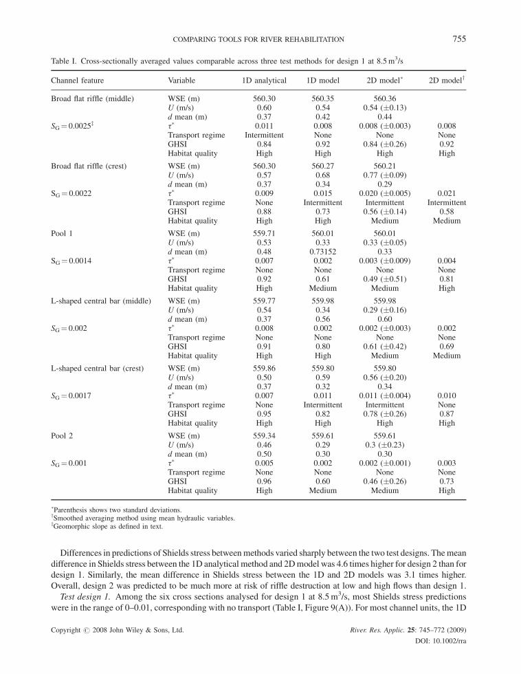
Table I. Cross-sectionally averaged values comparable across three test methods for design 1 at 8.5m3/s

Channel feature Variable 1D analytical 1D model 2D model� 2D modely

Broad flat riffle (middle) WSE (m) 560.30 560.35 560.36U (m/s) 0.60 0.54 0.54 (�0.13)d mean (m) 0.37 0.42 0.44

SG¼ 0.0025z t� 0.011 0.008 0.008 (�0.003) 0.008Transport regime Intermittent None None NoneGHSI 0.84 0.92 0.84 (�0.26) 0.92Habitat quality High High High High

Broad flat riffle (crest) WSE (m) 560.30 560.27 560.21U (m/s) 0.57 0.68 0.77 (�0.09)d mean (m) 0.37 0.34 0.29

SG¼ 0.0022 t� 0.009 0.015 0.020 (�0.005) 0.021Transport regime None Intermittent Intermittent IntermittentGHSI 0.88 0.73 0.56 (�0.14) 0.58Habitat quality High High Medium Medium

Pool 1 WSE (m) 559.71 560.01 560.01U (m/s) 0.53 0.33 0.33 (�0.05)d mean (m) 0.48 0.73152 0.33

SG¼ 0.0014 t� 0.007 0.002 0.003 (�0.009) 0.004Transport regime None None None NoneGHSI 0.92 0.61 0.49 (�0.51) 0.81Habitat quality High Medium Medium High

L-shaped central bar (middle) WSE (m) 559.77 559.98 559.98U (m/s) 0.54 0.34 0.29 (�0.16)d mean (m) 0.37 0.56 0.60

SG¼ 0.002 t� 0.008 0.002 0.002 (�0.003) 0.002Transport regime None None None NoneGHSI 0.91 0.80 0.61 (�0.42) 0.69Habitat quality High High Medium Medium

L-shaped central bar (crest) WSE (m) 559.86 559.80 559.80U (m/s) 0.50 0.59 0.56 (�0.20)d mean (m) 0.37 0.32 0.34

SG¼ 0.0017 t� 0.007 0.011 0.011 (�0.004) 0.010Transport regime None Intermittent Intermittent NoneGHSI 0.95 0.82 0.78 (�0.26) 0.87Habitat quality High High High High

Pool 2 WSE (m) 559.34 559.61 559.61U (m/s) 0.46 0.29 0.3 (�0.23)d mean (m) 0.50 0.30 0.30

SG¼ 0.001 t� 0.005 0.002 0.002 (�0.001) 0.003Transport regime None None None NoneGHSI 0.96 0.60 0.46 (�0.26) 0.73Habitat quality High Medium Medium High

�Parenthesis shows two standard deviations.ySmoothed averaging method using mean hydraulic variables.zGeomorphic slope as defined in text.

COMPARING TOOLS FOR RIVER REHABILITATION 755

Differences in predictions of Shields stress betweenmethods varied sharply between the two test designs. Themean

difference in Shields stress between the 1D analytical method and 2Dmodel was 4.6 times higher for design 2 than for

design 1. Similarly, the mean difference in Shields stress between the 1D and 2D models was 3.1 times higher.

Overall, design 2 was predicted to be much more at risk of riffle destruction at low and high flows than design 1.

Test design 1. Among the six cross sections analysed for design 1 at 8.5m3/s, most Shields stress predictions

were in the range of 0–0.01, corresponding with no transport (Table I, Figure 9(A)). For most channel units, the 1D

Copyright # 2008 John Wiley & Sons, Ltd. River. Res. Applic. 25: 745–772 (2009)

DOI: 10.1002/rra

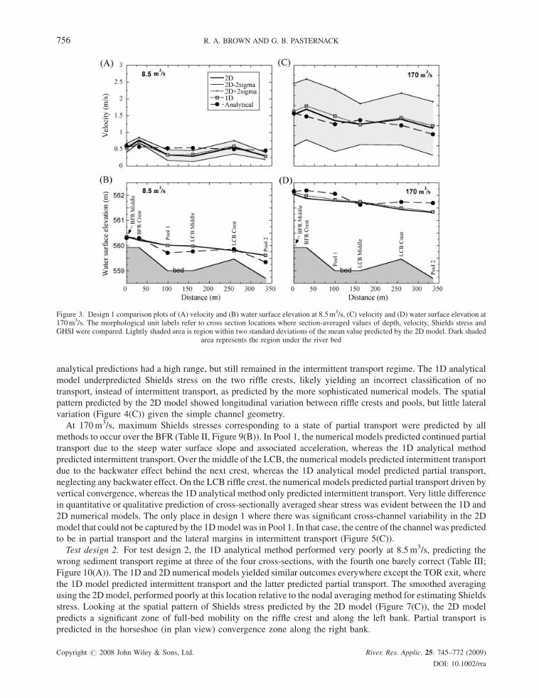
Figure 3. Design 1 comparison plots of (A) velocity and (B) water surface elevation at 8.5m3/s, (C) velocity and (D) water surface elevation at170m3/s. The morphological unit labels refer to cross section locations where section-averaged values of depth, velocity, Shields stress andGHSI were compared. Lightly shaded area is region within two standard deviations of the mean value predicted by the 2D model. Dark shaded

area represents the region under the river bed

756 R. A. BROWN AND G. B. PASTERNACK

analytical predictions had a high range, but still remained in the intermittent transport regime. The 1D analytical

model underpredicted Shields stress on the two riffle crests, likely yielding an incorrect classification of no

transport, instead of intermittent transport, as predicted by the more sophisticated numerical models. The spatial

pattern predicted by the 2D model showed longitudinal variation between riffle crests and pools, but little lateral

variation (Figure 4(C)) given the simple channel geometry.

At 170m3/s, maximum Shields stresses corresponding to a state of partial transport were predicted by all

methods to occur over the BFR (Table II, Figure 9(B)). In Pool 1, the numerical models predicted continued partial

transport due to the steep water surface slope and associated acceleration, whereas the 1D analytical method

predicted intermittent transport. Over the middle of the LCB, the numerical models predicted intermittent transport

due to the backwater effect behind the next crest, whereas the 1D analytical model predicted partial transport,

neglecting any backwater effect. On the LCB riffle crest, the numerical models predicted partial transport driven by

vertical convergence, whereas the 1D analytical method only predicted intermittent transport. Very little difference

in quantitative or qualitative prediction of cross-sectionally averaged shear stress was evident between the 1D and

2D numerical models. The only place in design 1 where there was significant cross-channel variability in the 2D

model that could not be captured by the 1Dmodel was in Pool 1. In that case, the centre of the channel was predicted

to be in partial transport and the lateral margins in intermittent transport (Figure 5(C)).

Test design 2. For test design 2, the 1D analytical method performed very poorly at 8.5m3/s, predicting the

wrong sediment transport regime at three of the four cross-sections, with the fourth one barely correct (Table III;

Figure 10(A)). The 1D and 2D numerical models yielded similar outcomes everywhere except the TOR exit, where

the 1D model predicted intermittent transport and the latter predicted partial transport. The smoothed averaging

using the 2Dmodel, performed poorly at this location relative to the nodal averaging method for estimating Shields

stress. Looking at the spatial pattern of Shields stress predicted by the 2D model (Figure 7(C)), the 2D model

predicts a significant zone of full-bed mobility on the riffle crest and along the left bank. Partial transport is

predicted in the horseshoe (in plan view) convergence zone along the right bank.

Copyright # 2008 John Wiley & Sons, Ltd. River. Res. Applic. 25: 745–772 (2009)

DOI: 10.1002/rra

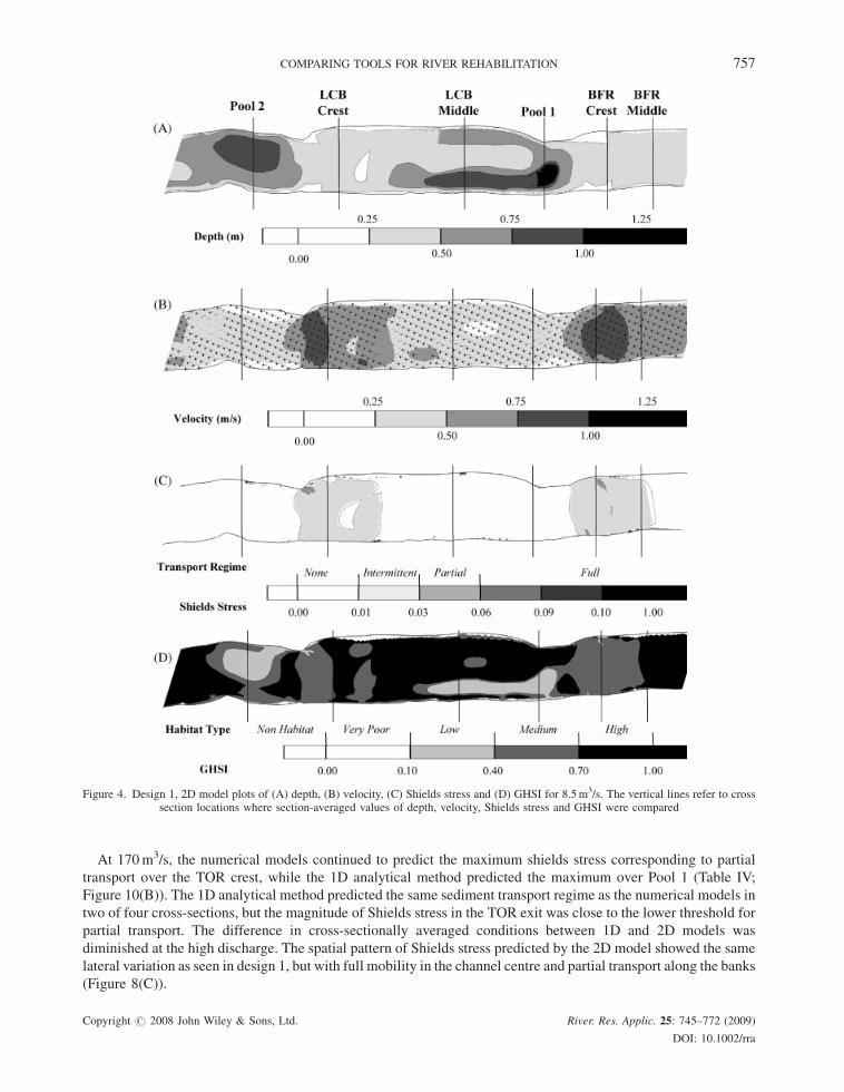
Figure 4. Design 1, 2D model plots of (A) depth, (B) velocity, (C) Shields stress and (D) GHSI for 8.5m3/s. The vertical lines refer to crosssection locations where section-averaged values of depth, velocity, Shields stress and GHSI were compared

COMPARING TOOLS FOR RIVER REHABILITATION 757

At 170m3/s, the numerical models continued to predict the maximum shields stress corresponding to partial

transport over the TOR crest, while the 1D analytical method predicted the maximum over Pool 1 (Table IV;

Figure 10(B)). The 1D analytical method predicted the same sediment transport regime as the numerical models in

two of four cross-sections, but the magnitude of Shields stress in the TOR exit was close to the lower threshold for

partial transport. The difference in cross-sectionally averaged conditions between 1D and 2D models was

diminished at the high discharge. The spatial pattern of Shields stress predicted by the 2D model showed the same

lateral variation as seen in design 1, but with full mobility in the channel centre and partial transport along the banks

(Figure 8(C)).

Copyright # 2008 John Wiley & Sons, Ltd. River. Res. Applic. 25: 745–772 (2009)

DOI: 10.1002/rra

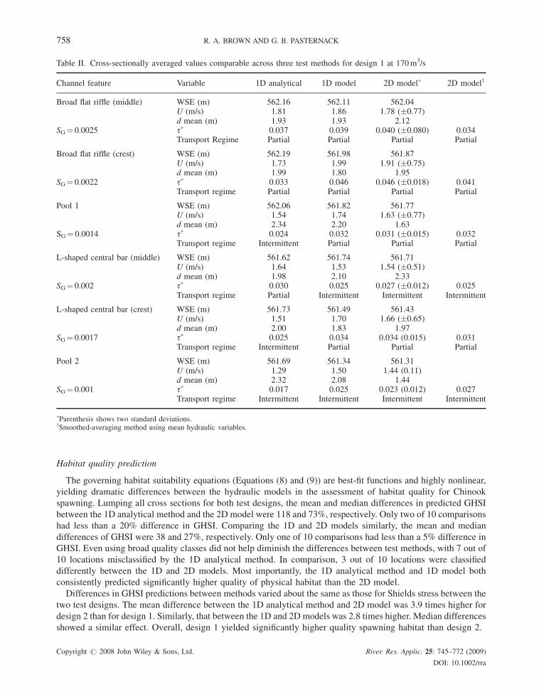
Table II. Cross-sectionally averaged values comparable across three test methods for design 1 at 170m3/s

Channel feature Variable 1D analytical 1D model 2D model� 2D modely

Broad flat riffle (middle) WSE (m) 562.16 562.11 562.04U (m/s) 1.81 1.86 1.78 (�0.77)d mean (m) 1.93 1.93 2.12

SG¼ 0.0025 t� 0.037 0.039 0.040 (�0.080) 0.034Transport Regime Partial Partial Partial Partial

Broad flat riffle (crest) WSE (m) 562.19 561.98 561.87U (m/s) 1.73 1.99 1.91 (�0.75)d mean (m) 1.99 1.80 1.95

SG¼ 0.0022 t� 0.033 0.046 0.046 (�0.018) 0.041Transport regime Partial Partial Partial Partial

Pool 1 WSE (m) 562.06 561.82 561.77U (m/s) 1.54 1.74 1.63 (�0.77)d mean (m) 2.34 2.20 1.63

SG¼ 0.0014 t� 0.024 0.032 0.031 (�0.015) 0.032Transport regime Intermittent Partial Partial Partial

L-shaped central bar (middle) WSE (m) 561.62 561.74 561.71U (m/s) 1.64 1.53 1.54 (�0.51)d mean (m) 1.98 2.10 2.33

SG¼ 0.002 t� 0.030 0.025 0.027 (�0.012) 0.025Transport regime Partial Intermittent Intermittent Intermittent

L-shaped central bar (crest) WSE (m) 561.73 561.49 561.43U (m/s) 1.51 1.70 1.66 (�0.65)d mean (m) 2.00 1.83 1.97

SG¼ 0.0017 t� 0.025 0.034 0.034 (0.015) 0.031Transport regime Intermittent Partial Partial Partial

Pool 2 WSE (m) 561.69 561.34 561.31U (m/s) 1.29 1.50 1.44 (0.11)d mean (m) 2.32 2.08 1.44

SG¼ 0.001 t� 0.017 0.025 0.023 (0.012) 0.027Transport regime Intermittent Intermittent Intermittent Intermittent

�Parenthesis shows two standard deviations.ySmoothed-averaging method using mean hydraulic variables.

758 R. A. BROWN AND G. B. PASTERNACK

Habitat quality prediction

The governing habitat suitability equations (Equations (8) and (9)) are best-fit functions and highly nonlinear,

yielding dramatic differences between the hydraulic models in the assessment of habitat quality for Chinook

spawning. Lumping all cross sections for both test designs, the mean and median differences in predicted GHSI

between the 1D analytical method and the 2D model were 118 and 73%, respectively. Only two of 10 comparisons

had less than a 20% difference in GHSI. Comparing the 1D and 2D models similarly, the mean and median

differences of GHSI were 38 and 27%, respectively. Only one of 10 comparisons had less than a 5% difference in

GHSI. Even using broad quality classes did not help diminish the differences between test methods, with 7 out of

10 locations misclassified by the 1D analytical method. In comparison, 3 out of 10 locations were classified

differently between the 1D and 2D models. Most importantly, the 1D analytical method and 1D model both

consistently predicted significantly higher quality of physical habitat than the 2D model.

Differences in GHSI predictions between methods varied about the same as those for Shields stress between the

two test designs. The mean difference between the 1D analytical method and 2D model was 3.9 times higher for

design 2 than for design 1. Similarly, that between the 1D and 2D models was 2.8 times higher. Median differences

showed a similar effect. Overall, design 1 yielded significantly higher quality spawning habitat than design 2.

Copyright # 2008 John Wiley & Sons, Ltd. River. Res. Applic. 25: 745–772 (2009)

DOI: 10.1002/rra

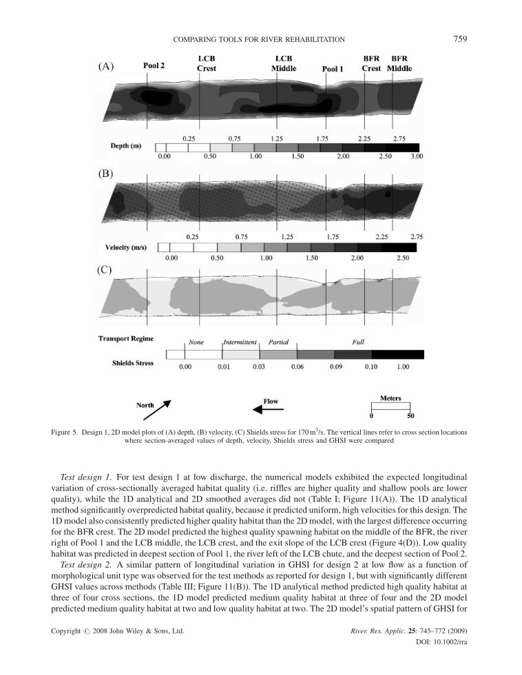
Figure 5. Design 1, 2D model plots of (A) depth, (B) velocity, (C) Shields stress for 170m3/s. The vertical lines refer to cross section locationswhere section-averaged values of depth, velocity, Shields stress and GHSI were compared

COMPARING TOOLS FOR RIVER REHABILITATION 759

Test design 1. For test design 1 at low discharge, the numerical models exhibited the expected longitudinal

variation of cross-sectionally averaged habitat quality (i.e. riffles are higher quality and shallow pools are lower

quality), while the 1D analytical and 2D smoothed averages did not (Table I; Figure 11(A)). The 1D analytical

method significantly overpredicted habitat quality, because it predicted uniform, high velocities for this design. The

1Dmodel also consistently predicted higher quality habitat than the 2Dmodel, with the largest difference occurring

for the BFR crest. The 2D model predicted the highest quality spawning habitat on the middle of the BFR, the river

right of Pool 1 and the LCB middle, the LCB crest, and the exit slope of the LCB crest (Figure 4(D)). Low quality

habitat was predicted in deepest section of Pool 1, the river left of the LCB chute, and the deepest section of Pool 2.

Test design 2. A similar pattern of longitudinal variation in GHSI for design 2 at low flow as a function of

morphological unit type was observed for the test methods as reported for design 1, but with significantly different

GHSI values across methods (Table III; Figure 11(B)). The 1D analytical method predicted high quality habitat at

three of four cross sections, the 1D model predicted medium quality habitat at three of four and the 2D model

predicted medium quality habitat at two and low quality habitat at two. The 2D model’s spatial pattern of GHSI for

Copyright # 2008 John Wiley & Sons, Ltd. River. Res. Applic. 25: 745–772 (2009)

DOI: 10.1002/rra

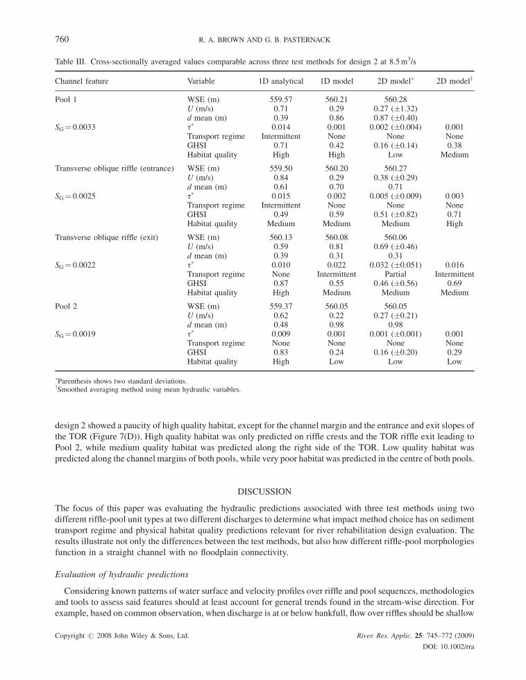
Table III. Cross-sectionally averaged values comparable across three test methods for design 2 at 8.5m3/s

Channel feature Variable 1D analytical 1D model 2D model� 2D modely

Pool 1 WSE (m) 559.57 560.21 560.28U (m/s) 0.71 0.29 0.27 (�1.32)d mean (m) 0.39 0.86 0.87 (�0.40)

SG¼ 0.0033 t� 0.014 0.001 0.002 (�0.004) 0.001Transport regime Intermittent None None NoneGHSI 0.71 0.42 0.16 (�0.14) 0.38Habitat quality High High Low Medium

Transverse oblique riffle (entrance) WSE (m) 559.50 560.20 560.27U (m/s) 0.84 0.29 0.38 (�0.29)d mean (m) 0.61 0.70 0.71

SG¼ 0.0025 t� 0.015 0.002 0.005 (�0.009) 0.003Transport regime Intermittent None None NoneGHSI 0.49 0.59 0.51 (�0.82) 0.71Habitat quality Medium Medium Medium High

Transverse oblique riffle (exit) WSE (m) 560.13 560.08 560.06U (m/s) 0.59 0.81 0.69 (�0.46)d mean (m) 0.39 0.31 0.31

SG¼ 0.0022 t� 0.010 0.022 0.032 (�0.051) 0.016Transport regime None Intermittent Partial IntermittentGHSI 0.87 0.55 0.46 (�0.56) 0.69Habitat quality High Medium Medium Medium

Pool 2 WSE (m) 559.37 560.05 560.05U (m/s) 0.62 0.22 0.27 (�0.21)d mean (m) 0.48 0.98 0.98

SG¼ 0.0019 t� 0.009 0.001 0.001 (�0.001) 0.001Transport regime None None None NoneGHSI 0.83 0.24 0.16 (�0.20) 0.29Habitat quality High Low Low Low

�Parenthesis shows two standard deviations.ySmoothed averaging method using mean hydraulic variables.

760 R. A. BROWN AND G. B. PASTERNACK

design 2 showed a paucity of high quality habitat, except for the channel margin and the entrance and exit slopes of

the TOR (Figure 7(D)). High quality habitat was only predicted on riffle crests and the TOR riffle exit leading to

Pool 2, while medium quality habitat was predicted along the right side of the TOR. Low quality habitat was

predicted along the channel margins of both pools, while very poor habitat was predicted in the centre of both pools.

DISCUSSION

The focus of this paper was evaluating the hydraulic predictions associated with three test methods using two

different riffle-pool unit types at two different discharges to determine what impact method choice has on sediment

transport regime and physical habitat quality predictions relevant for river rehabilitation design evaluation. The

results illustrate not only the differences between the test methods, but also how different riffle-pool morphologies

function in a straight channel with no floodplain connectivity.

Evaluation of hydraulic predictions

Considering known patterns of water surface and velocity profiles over riffle and pool sequences, methodologies

and tools to assess said features should at least account for general trends found in the stream-wise direction. For

example, based on common observation, when discharge is at or below bankfull, flow over riffles should be shallow

Copyright # 2008 John Wiley & Sons, Ltd. River. Res. Applic. 25: 745–772 (2009)

DOI: 10.1002/rra

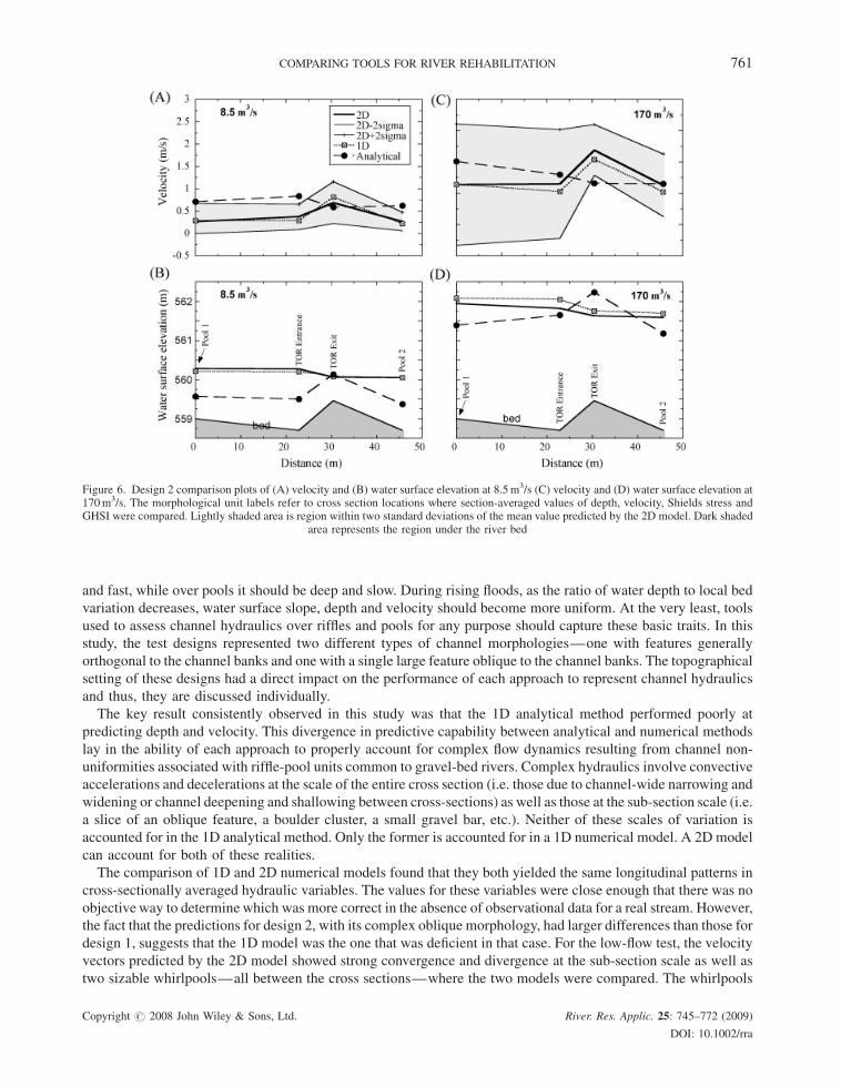
Figure 6. Design 2 comparison plots of (A) velocity and (B) water surface elevation at 8.5m3/s (C) velocity and (D) water surface elevation at170m3/s. The morphological unit labels refer to cross section locations where section-averaged values of depth, velocity, Shields stress andGHSI were compared. Lightly shaded area is region within two standard deviations of the mean value predicted by the 2D model. Dark shaded

area represents the region under the river bed

COMPARING TOOLS FOR RIVER REHABILITATION 761

and fast, while over pools it should be deep and slow. During rising floods, as the ratio of water depth to local bed

variation decreases, water surface slope, depth and velocity should become more uniform. At the very least, tools

used to assess channel hydraulics over riffles and pools for any purpose should capture these basic traits. In this

study, the test designs represented two different types of channel morphologies—one with features generally

orthogonal to the channel banks and one with a single large feature oblique to the channel banks. The topographical

setting of these designs had a direct impact on the performance of each approach to represent channel hydraulics

and thus, they are discussed individually.

The key result consistently observed in this study was that the 1D analytical method performed poorly at

predicting depth and velocity. This divergence in predictive capability between analytical and numerical methods

lay in the ability of each approach to properly account for complex flow dynamics resulting from channel non-

uniformities associated with riffle-pool units common to gravel-bed rivers. Complex hydraulics involve convective

accelerations and decelerations at the scale of the entire cross section (i.e. those due to channel-wide narrowing and

widening or channel deepening and shallowing between cross-sections) as well as those at the sub-section scale (i.e.

a slice of an oblique feature, a boulder cluster, a small gravel bar, etc.). Neither of these scales of variation is

accounted for in the 1D analytical method. Only the former is accounted for in a 1D numerical model. A 2D model

can account for both of these realities.

The comparison of 1D and 2D numerical models found that they both yielded the same longitudinal patterns in

cross-sectionally averaged hydraulic variables. The values for these variables were close enough that there was no

objectiveway to determine which was more correct in the absence of observational data for a real stream. However,

the fact that the predictions for design 2, with its complex oblique morphology, had larger differences than those for

design 1, suggests that the 1D model was the one that was deficient in that case. For the low-flow test, the velocity

vectors predicted by the 2D model showed strong convergence and divergence at the sub-section scale as well as

two sizable whirlpools—all between the cross sections—where the two models were compared. The whirlpools

Copyright # 2008 John Wiley & Sons, Ltd. River. Res. Applic. 25: 745–772 (2009)

DOI: 10.1002/rra

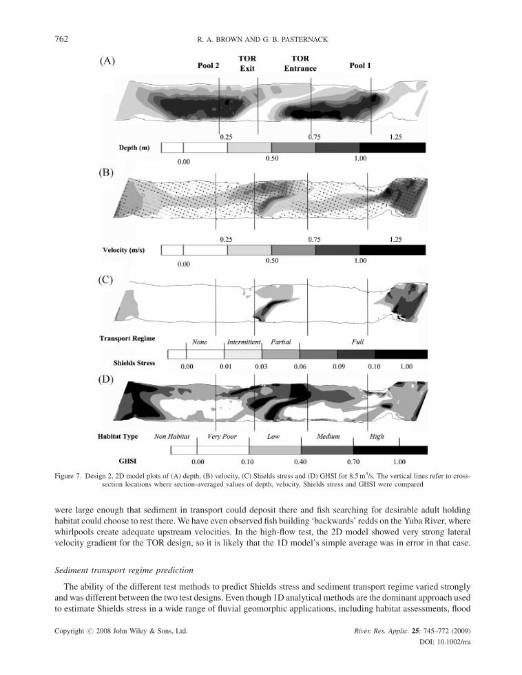
Figure 7. Design 2, 2D model plots of (A) depth, (B) velocity, (C) Shields stress and (D) GHSI for 8.5m3/s. The vertical lines refer to cross-section locations where section-averaged values of depth, velocity, Shields stress and GHSI were compared

762 R. A. BROWN AND G. B. PASTERNACK

were large enough that sediment in transport could deposit there and fish searching for desirable adult holding

habitat could choose to rest there. We have even observed fish building ‘backwards’ redds on the Yuba River, where

whirlpools create adequate upstream velocities. In the high-flow test, the 2D model showed very strong lateral

velocity gradient for the TOR design, so it is likely that the 1D model’s simple average was in error in that case.

Sediment transport regime prediction

The ability of the different test methods to predict Shields stress and sediment transport regime varied strongly

and was different between the two test designs. Even though 1D analytical methods are the dominant approach used

to estimate Shields stress in a wide range of fluvial geomorphic applications, including habitat assessments, flood

Copyright # 2008 John Wiley & Sons, Ltd. River. Res. Applic. 25: 745–772 (2009)

DOI: 10.1002/rra

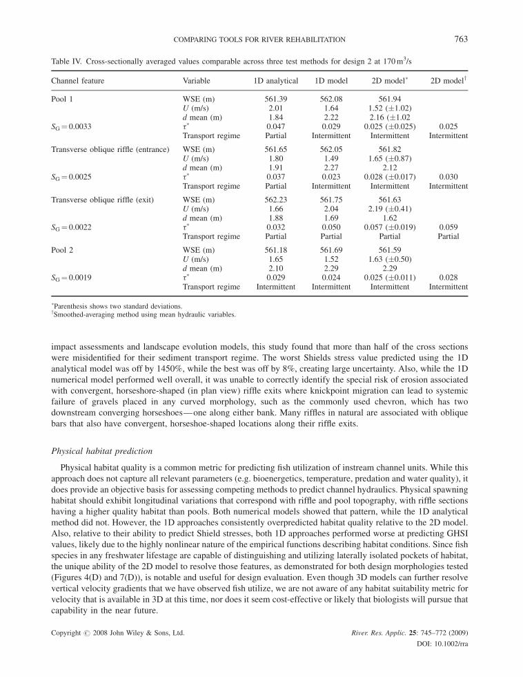
Table IV. Cross-sectionally averaged values comparable across three test methods for design 2 at 170m3/s

Channel feature Variable 1D analytical 1D model 2D model� 2D modely

Pool 1 WSE (m) 561.39 562.08 561.94U (m/s) 2.01 1.64 1.52 (�1.02)d mean (m) 1.84 2.22 2.16 (�1.02

SG¼ 0.0033 t� 0.047 0.029 0.025 (�0.025) 0.025Transport regime Partial Intermittent Intermittent Intermittent

Transverse oblique riffle (entrance) WSE (m) 561.65 562.05 561.82U (m/s) 1.80 1.49 1.65 (�0.87)d mean (m) 1.91 2.27 2.12

SG¼ 0.0025 t� 0.037 0.023 0.028 (�0.017) 0.030Transport regime Partial Intermittent Intermittent Intermittent

Transverse oblique riffle (exit) WSE (m) 562.23 561.75 561.63U (m/s) 1.66 2.04 2.19 (�0.41)d mean (m) 1.88 1.69 1.62

SG¼ 0.0022 t� 0.032 0.050 0.057 (�0.019) 0.059Transport regime Partial Partial Partial Partial

Pool 2 WSE (m) 561.18 561.69 561.59U (m/s) 1.65 1.52 1.63 (�0.50)d mean (m) 2.10 2.29 2.29

SG¼ 0.0019 t� 0.029 0.024 0.025 (�0.011) 0.028Transport regime Intermittent Intermittent Intermittent Intermittent

�Parenthesis shows two standard deviations.ySmoothed-averaging method using mean hydraulic variables.

COMPARING TOOLS FOR RIVER REHABILITATION 763

impact assessments and landscape evolution models, this study found that more than half of the cross sections

were misidentified for their sediment transport regime. The worst Shields stress value predicted using the 1D

analytical model was off by 1450%, while the best was off by 8%, creating large uncertainty. Also, while the 1D

numerical model performed well overall, it was unable to correctly identify the special risk of erosion associated

with convergent, horseshore-shaped (in plan view) riffle exits where knickpoint migration can lead to systemic

failure of gravels placed in any curved morphology, such as the commonly used chevron, which has two

downstream converging horseshoes—one along either bank. Many riffles in natural are associated with oblique

bars that also have convergent, horseshoe-shaped locations along their riffle exits.

Physical habitat prediction

Physical habitat quality is a common metric for predicting fish utilization of instream channel units. While this

approach does not capture all relevant parameters (e.g. bioenergetics, temperature, predation and water quality), it

does provide an objective basis for assessing competing methods to predict channel hydraulics. Physical spawning

habitat should exhibit longitudinal variations that correspond with riffle and pool topography, with riffle sections

having a higher quality habitat than pools. Both numerical models showed that pattern, while the 1D analytical

method did not. However, the 1D approaches consistently overpredicted habitat quality relative to the 2D model.

Also, relative to their ability to predict Shield stresses, both 1D approaches performed worse at predicting GHSI

values, likely due to the highly nonlinear nature of the empirical functions describing habitat conditions. Since fish

species in any freshwater lifestage are capable of distinguishing and utilizing laterally isolated pockets of habitat,

the unique ability of the 2D model to resolve those features, as demonstrated for both design morphologies tested

(Figures 4(D) and 7(D)), is notable and useful for design evaluation. Even though 3D models can further resolve

vertical velocity gradients that we have observed fish utilize, we are not aware of any habitat suitability metric for

velocity that is available in 3D at this time, nor does it seem cost-effective or likely that biologists will pursue that

capability in the near future.

Copyright # 2008 John Wiley & Sons, Ltd. River. Res. Applic. 25: 745–772 (2009)

DOI: 10.1002/rra

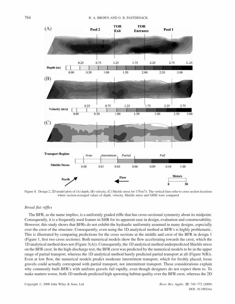
Figure 8. Design 2, 2D model plots of (A) depth, (B) velocity, (C) Shields stress for 170m3/s. The vertical lines refer to cross section locationswhere section-averaged values of depth, velocity, Shields stress and GHSI were compared

764 R. A. BROWN AND G. B. PASTERNACK

Broad flat riffles

The BFR, as the name implies, is a uniformly graded riffle that has cross-sectional symmetry about its midpoint.

Consequently, it is a frequently used feature in SHR for its apparent ease in design, evaluation and constructability.

However, this study shows that BFRs do not exhibit the hydraulic uniformity assumed in many designs, especially

over the crest of the structure. Consequently, even using the 1D analytical method at BFR’s is highly problematic.

This is illustrated by comparing predictions for the cross sections at the middle and crest of the BFR in design 1

(Figure 1, first two cross sections). Both numerical models show the flow accelerating towards the crest, which the

1D analytical method does not (Figure 3(A)). Consequently, the 1D analytical method underpredicted Shields stress

on the BFR crest. In the high-discharge test, the BFR crest was predicted by the numerical models to be in the upper

range of partial transport, whereas the 1D analytical method barely predicted partial transport at all (Figure 9(B)).

Even at low flow, the numerical models predict moderate intermittent transport, which for freshly placed, loose

gravels could actually correspond with partial transport, not intermittent transport. These considerations explain

why commonly built BFR’s with uniform gravels fail rapidly, even though designers do not expect them to. To

make matters worse, both 1D methods predicted high spawning habitat quality over the BFR crest, whereas the 2D

Copyright # 2008 John Wiley & Sons, Ltd. River. Res. Applic. 25: 745–772 (2009)

DOI: 10.1002/rra

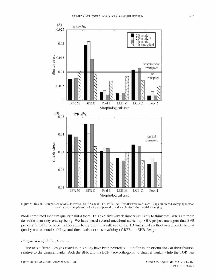
Figure 9. Design 1 comparison of Shields stress at (A) 8.5 and (B) 170m3/s. The ‘�’ results were calculated using a smoothed averaging methodbased on mean depth and velocity as opposed to values obtained from nodal averaging

COMPARING TOOLS FOR RIVER REHABILITATION 765

model predicted medium quality habitat there. This explains why designers are likely to think that BFR’s are more

desirable than they end up being. We have heard several anecdotal stories by SHR project managers that BFR

projects failed to be used by fish after being built. Overall, use of the 1D analytical method overpredicts habitat

quality and channel stability, and thus leads to an overvaluing of BFRs in SHR design.

Comparison of design features

The two different designs tested in this study have been pointed out to differ in the orientations of their features

relative to the channel banks. Both the BFR and the LCF were orthogonal to channel banks, while the TOR was

Copyright # 2008 John Wiley & Sons, Ltd. River. Res. Applic. 25: 745–772 (2009)

DOI: 10.1002/rra

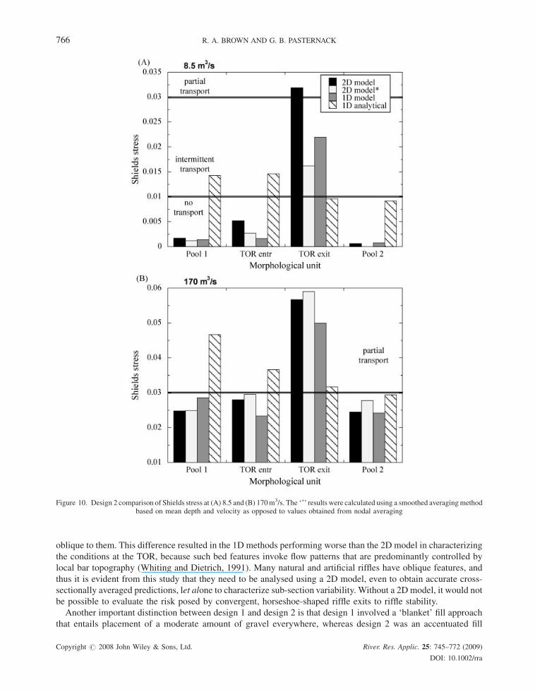
Figure 10. Design 2 comparison of Shields stress at (A) 8.5 and (B) 170m3/s. The ‘�’ results were calculated using a smoothed averagingmethodbased on mean depth and velocity as opposed to values obtained from nodal averaging

766 R. A. BROWN AND G. B. PASTERNACK

oblique to them. This difference resulted in the 1D methods performing worse than the 2D model in characterizing

the conditions at the TOR, because such bed features invoke flow patterns that are predominantly controlled by

local bar topography (Whiting and Dietrich, 1991). Many natural and artificial riffles have oblique features, and

thus it is evident from this study that they need to be analysed using a 2D model, even to obtain accurate cross-

sectionally averaged predictions, let alone to characterize sub-section variability. Without a 2D model, it would not

be possible to evaluate the risk posed by convergent, horseshoe-shaped riffle exits to riffle stability.

Another important distinction between design 1 and design 2 is that design 1 involved a ‘blanket’ fill approach

that entails placement of a moderate amount of gravel everywhere, whereas design 2 was an accentuated fill

Copyright # 2008 John Wiley & Sons, Ltd. River. Res. Applic. 25: 745–772 (2009)

DOI: 10.1002/rra

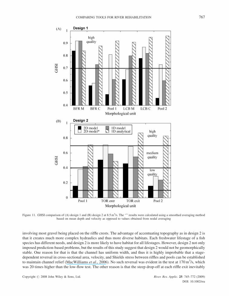
Figure 11. GHSI comparison of (A) design 1 and (B) design 2 at 8.5m3/s. The ‘�’ results were calculated using a smoothed averaging methodbased on mean depth and velocity as opposed to values obtained from nodal averaging

COMPARING TOOLS FOR RIVER REHABILITATION 767

involving most gravel being placed on the riffle crests. The advantage of accentuating topography as in design 2 is

that it creates much more complex hydraulics and thus more diverse habitats. Each freshwater lifestage of a fish

species has different needs, and design 2 is more likely to have habitat for all lifestages. However, design 2 not only

imposed prediction-based problems, but the results of this study suggest that design 2 would not be geomorphically

stable. One reason for that is that the channel has uniform width, and thus it is highly improbable that a stage-

dependent reversal in cross-sectional area, velocity, and Shields stress between riffles and pools can be established

to maintain channel relief (MacWilliams et al., 2006). No such reversal was evident in the test at 170m3/s, which

was 20 times higher than the low-flow test. The other reason is that the steep drop-off at each riffle exit inevitably

Copyright # 2008 John Wiley & Sons, Ltd. River. Res. Applic. 25: 745–772 (2009)

DOI: 10.1002/rra

768 R. A. BROWN AND G. B. PASTERNACK

creates excessive velocities and localized bed scour. This can cause knickpoint migration that can quickly cut

through the entire feature. Such an effect was observed for the 2001 project site on the lower Mokelumne River

(Merz et al., 2006) when less gravel was provided than called for bythe design of Wheaton et al. (2004b), resulting

in a steep, horse-shoe shaped riffle exit at the downstream end of the project site. For the actual SHR project on the

Trinity River, a thorough analysis was done for three different accentuated-relief designs and three different

blanket-fill designs. In the end, the selected design was a blanket-fill morphology using one broad flat riffle and two

L-shaped bars. Details of all these designs and their evaluations are available at http://shira.lawr.ucdavis.edu/

trinity.htm.

Implications to SHR design and decision making

Decision making for river management often relies on model predictions of physical habitat to forecast potential

impacts of flow regime changes as well as for evaluating potential gravel augmentation designs. In this study a

sediment transport regime metric and a global habitat suitability index were used to transform quantitative

hydraulic predictions into relevant qualitative descriptors of geomorphic and ecologic conditions. Deviations in

hydraulic predictions led to contrasting results for section-average Shields stress and GHSI for each test design,

ultimately being related to whether the topography of the features initiated cross-stream flow vectors and lateral

variation in stream-wise vectors that deviated from cross-sectionally averaged estimates.

Manning’s equation and other analytical flow resistance equations are often considered adequate for engineering

tasks involving open channel flows in deep channels with a high depth to bed-feature height ratio (>100–1000 as a

conservative estimate). In this study, that ratio ranged from�1 to 10. The results of this study show that for shallow

gravel-bed rivers with complex morphologies, including common river rehabilitation design structures of simple

geometry, the 1D analytical method is inappropriate for estimating depth and velocity. These limitations can be

further assumed to affect any non-uniform channel section with a width to depth ratio in this range, and probably up

to at least 50. Despite this inadequacy, there is a practice of ‘fine-tuning’ Manning’s equation using detailed

accounting of roughness in the channel and velocity-profile effects. The benefits of these and other attempts to bend

Manning equation to fit the desire for a simple method are unlikely to be of use for SHR design evaluation.

The results of this study suggest that a river manager, policy maker, scientist or engineer faced with evaluating

the effect of a potential gravel augmentation design, a channel modification or a flow regime change on physical

habitat would come to very different conclusions depending on whether the hydraulics of the channel were

evaluated using Manning’s equation or a 1D or 2D numerical model. The quality of spawning habitat was

consistently over predicted by 1D methods. Moreover, considering reach scale (102–103 channel widths) averages

of spawning habitat quality by averaging GHSI among sections for both designs, 1D methods still grossly over-

predict habitat such that medium and low quality habitat would be predicted as high quality habitat. As 1D reach-

scale approaches to physical habitat are the most prevalent, this could lead decision makers to believe that existing

and proposed physical habitat is of higher quality and quantity, leading to false conclusions about river health.

Considering the rapid decline of salmonids despite the known linkages to habitat degradation, it is not implausible

to postulate these over-predictions of existing and proposed physical habitat have already manifested themselves

into key management plans of gravel bed rivers and dam re-licensing.

Predictions regarding channel stability and sediment transport would be impacted as well from using analytical

or numerically based tools. Under predicting Shields stress over riffle crests could be catastrophic to SHR based

gravel augmentation as knickpoint migration at the riffle crest could lead to systemic failure, especially for a

sequence of riffle crests, which could experience a ‘reverse domino’ toppling of bedforms (Pasternack et al.,

in press). Moreover, small areas of high stress may be present that no section averaged approach can capture.

Failure to identify these areas could also lead to riffle failure.

CONCLUSIONS

Typical goals of most spawning habitat rehabilitation projects involve increasing quantity and quality of one or

more life stages of a species. Placed gravels must be stable during low discharges to avoid embryo mortality and

have some sediment transport at high discharges to rejuvenate gravels by removing aquatic vegetation and

Copyright # 2008 John Wiley & Sons, Ltd. River. Res. Applic. 25: 745–772 (2009)

DOI: 10.1002/rra

COMPARING TOOLS FOR RIVER REHABILITATION 769

interstitial fines. Generally speaking, a project is considered successful if the number of redds and consequent fry

production increases and the project is stable during the spawning and incubation seasons, with some transport

during large flow events after incubation. Therefore, the evaluation of potential designs rests on two key

parameters—sediment transport regime and physical habitat quality. In this study, three methods were tested

against two different channel morphologies at two different discharges. Numerical models captured the general

stream-wise hydraulics associated with riffles and pools that a 1D analytically method could not predict. Failure to

account for convective accelerations within and between riffles and pools explains why the 1D analytical method

was wrong in most of its predictions. Although 1D and 2D numerical predictions of cross-sectionally averaged

values had good agreement for both designs at both discharges, significant variations in between cross-sections and

at the sub-section scale were not resolved by the 1D model. For example, the 2D model properly predicted the

presence of whirlpools and zones of convergent flow in horseshoe-shaped riffle exits. For spatially distributed

phenomena such as patterns of sediment erosion and fish habitat quality, it is highly recommended that 2D models

be used to resolve lateral variations, without which 1Dmodels appear to over-predict habitat quality, affecting long-

term river management policies and practices.

ACKNOWLEDGEMENTS

Financial support for this work was provided by USBR Award #03FG230766 and USFWS Agreement

DCN#113322G003 awarded by CALFED. We gratefully thank and acknowledge Eve Elkins, Marisa Escobar,

Peng Gao, Mark Grismer, Joe Merz, Hamish Moir, Jeff Mount and Joe Wheaton for their input on this manuscript.

We thank Michael Bounrisavong and Kaushal Parikh for their help on technical modelling issues. We thank Carlos

Alvarado, Evan Buckland, Cameron Poya and Dave Van Herick for field assistance.

REFERENCES

Andrews ED, Nankervis JM. 1995. Effective discharge and the design of channel maintenance flows for gravel-bed rivers. In Natural and

Anthropogenic Influences in Fluvial Geomorphology, Costa JE, Miller AJ, Potter KW, Wilcock PR (eds). American Geophysical Union:

Washington DC; 151–164.

Babkaiff S, Hay D, Fromouth C. 1997. Rehabilitating stream banks. In Fish Rehabilitation Procedures, Slaney PA, Zaldokas PA (eds). Ministry

of Environment, Lands and Parks: Vancouver, BC. Chapter 6, pp. 6–1, 6–23.

Bates PD, Anderson MG, Baird L, Walling DE, Simm D. 1992. Modeling floodplain flow with a two-dimensional finite element scheme. Earth

Surface Processes and Landforms 17: 575–588.

Bjornn TC, Reiser DW. 1991. Habitat requirements of salmonids in streams. In Influences of Forest and Rangeland Management on Salmonid

Fishes and Their Habitats, Meehan WR (ed.). American Fisheries Society: Bethesda, MD, 83–138, American Fisheries Society Special

Pubication 19.

Booker DJ, Sear DA, Payne AJ. 2001. Modeling three-dimensional flow structures and patterns of boundary shear stress in a natural pool-riffle

sequence. Earth Surface Processes and Landforms 26: 553–576.

Bovee KD, Lamb BL, Bartholow JM, Stalnaker CB, Taylor J, Henriksen J. 1998. Stream habitat analysis using the instream flow incremental

methodology. United States Geological Survey, Information and Technology Report USGS/BRD/ITR-1998-0004. Fort Collins, CO.

BrayshawAC. 1985. Bed microtopography and entrainment thresholds in gravel bed rivers.Geological Society of America Bulletin 96: 218–223.

Brown RA, Pasternack GB. 2008. Engineered channel controls limiting spawning habitat rehabilitation. Geomorphology 97: 631–654.

Brunner GW. 1998. HEC-RAS: River Analysis System. Unpublished Users Manual, Version 2.2. U.S. Army Corps of Engineers, CA.

Buffington JM, Lisle TE, Woodsmith RD, Hilton S. 2002. Controls on the size and occurrence of pools in coarse-grained forest rivers. River

Research and Applications 18: 507–531.

California Department of Fish and Game. 1998. California Salmonid Stream Habitat Restoration Manual, 3rd edition.

California Department of Water Resources. 2000. Merced River Robinson-Gallo Project—Ratzlaff Reach Engineering Report.

Cao Z, Carling PA. 2002. Mathematical modeling of alluvial rivers: reality and myth. Part 1: general overview.Water and Maritime Engineering

154: 207–219.

Cao Z, Carling P, Oakey R. 2003. Flow reversal over a natural pool-riffle sequence: a computational study. Earth Surface Processes and

Landforms 28: 689–705.

Carling PA. 1991. An appraisal of the velocity-reversal hypothesis for stable pool-riffle sequences in the river Severn, England. Earth Surface

Processes and Landforms 16: 19–31.

Copyright # 2008 John Wiley & Sons, Ltd. River. Res. Applic. 25: 745–772 (2009)

DOI: 10.1002/rra

770 R. A. BROWN AND G. B. PASTERNACK

Cederholm JC, Dominguez LG, Bumstead TW. 1997. Rehabilitating stream channels and fish habitat using large woody debris. In Fish

Rehabilitation Procedures, Slaney PA, Zaldokas PA (eds).Ministry of Environment, Lands and Parks: Vancouver, BC. Chapter 8, pp. 8–1, 8–28.

Chang HH. 1998. Fluvial Processes in River Engineering. John Wiley and Sons: New York, NY.

Clifford NJ, Richard KS. 1992. The reversal hypothesis and the maintenance of riffle-pool sequences: a review and field appraisal. In Lowland

Floodplain Rivers: Geomorphological Perspectives, Carling PA, Petts J (eds). Wiley and Sons: USA; 43–70.

Constantine CR,Mount JF, Florsheim JL. 2003. The effects of longitudinal differences in gravel mobility on the downstream fining pattern in the

Cosumnes river, California. The Journal of Geology 11: 233–241.

Copeland RR, Hall BN. 1998. Channel restoration design procedure. Engineering approaches to ecosystem restoration. Proceedings of 1998

Wetlands and River Restoration Conference, Reston, VA.

Darby SE, Van de Wiel MJ. 2003. Models in fluvial geomorphology. In Tools in Fluvial Geomorphology, Kondolf GM, Piegay H (eds). Wiley:

Chichester; 503–539.

DietrichWE,Whiting P. 1989. Boundary shear stress and sediment transport in river meanders of sand and gravel. In River Meandering, Ikeda S,

Parker G (eds). American Geophysical Union: Washington, DC; 1–50, Water Resources Monograph 12.

Dunne T, Leopold LB. 1987. Water in Environmental Planning. W.H. Freeman: San Francisco, CA.

Elkins EM, Pasternack GB, Merz JE. 2007. The use of slope creation for rehabilitating incised, regulated, gravel-bed rivers. Water Resources

Research. DOI:10.1029/2006WR005159

Fischer HB, List JE, Koh CR, Imberger J, Brooks NH. 1979. Mixing in Inland and Coastal Waters. Academic Press, Inc: New York, NY.

French JR, Clifford NJ. 2000. Hydrodynamic modeling as a basis for explaining estuarine environmental dynamics: some computational and

methodological issues. Hydrological Processes 14: 2089–2108.

Froehlich DC. 1989. HW031.D—finite element surface-water modeling system: two- dimensional flow in a horizontal plane-users manual.

Federal Highway Administration. Report FHWA-RD-88-17. Federal Highway Administration: Washington DC.

Gard M. 2006. Modeling changes in salmon spawning and rearing habitat associated with river channel restoration. International Journal of

River Basin Management 4: 1–11.

Ghanem A, Steffler P, Hicks F. 1996. Two-dimensional hydraulic simulation of physical habitat conditions in flowing streams. Regulated Rivers

Research and Management 12: 185–200.

Graf WL. 1996. Geomorphology and policy for restoration of impounded american rivers: what is ’natural?’. In The Scientific Nature of

Geomorphology: Proceedings of the 27th Binghamton Symposium in Geomorphology, Rhoads BL, Thorn CE (eds). JohnWiley & Sons Ltd.:

USA. pp. 443–473.

Graf WL. 2001. Damage control: dams and the physical integrity of america’s rivers. Annals of the Association of American Geographers 91: 1–

27.

Grant GE, Schmidt JC, Lewis SL. 2003. A geological framework for interpreting downstream effects of dams on rivers. In A Peculiar River,

O’Connor JE, Grant GE (eds). American Geophysical Union: 209–225.

Gray DH, Leiser AT. 1982. Biotechnical Slope Protection and Erosion Control. Van Nostrand Reinhold Company: New York, NY.

Harper D, Ebrahimnezhad M, Cot FCI. 1998. Artificial riffles in river rehabilitation: setting the goals and measuring the successes. Aquatic

Conservation-Marine and Freshwater Ecosystems 8: 5–16.

Harrison LR, Keller EA. 2007. Modeling forced pool–riffle hydraulics in a boulder-bed stream, southern California. Geomorphology 83: 232–

248.

Hunter CJ. 1991. Better Trout Habitat: A Guide to Stream Restoration and Management, Montana Land Alliance. Island Press: New York, NY.

Jacobson RB, Galat DL. 2006. Flow and form in rehabilitation of large-river ecosystems—an example from the lower Missouri river.

Geomorphology 77: 249–269.

Jowett IG. 1997. Instream flow methods: a comparison of approaches. Regulated Rivers Research and Management 13: 115–127.

Keller EA. 1971. Areal sorting of bed-load material; the hypothesis of velocity reversal. GSA Bulletin 82: 753–756.

Keller EA, Florsheim JL. 1993. Velocity-reversal hypothesis: a model approach. Earth Surface Processes and Landforms 18: 733–740.

Knighton AD. 1998. Fluvial Forms and Processes: A New Perspective. Arnold, London.

Kondolf GM. 1997. Hungry water: effects of dams and gravel mining on river channels. Environmental Management 21: 533–551.

Kondolf GM. 2000. Some suggested guidelines for geomorphic aspects of anadromous salmonid habitat restoration proposals. Restoration

Ecology 8: 48–56.

Kondolf GM, Vick JC, Ramirez TM. 1996. Salmon spawning habitat rehabilitation on the Merced river, California: an evaluation of project

planning and performance. Transactions of the American Fisheries Society 125: 899–912.

Lacey RW, Millar RG. 2004. Reach scale hydraulic assessment of instream salmonid habitat restoration. Journal of the American Water

Resources Association 40: 1631–1644.

Leclerc M, Boudreault A, Bechara JA, Corfa G. 1995. 2-Dimensional hydrodynamic modeling—a neglected tool in the instream flow

incremental methodology. Transactions of the American Fisheries Society 124: 645–662.

Leopold LB, Maddock T. 1953. The hydraulic geometry of stream channels and some physiographic implications. United States Geological

Survey Professional Paper 252.

Leopold LB, Wolman MG, Miller JP. 1964. Fluvial Processes in Geomorphology. W.H. Freeman and Company: San Francisco, CA.

Lisle T. 1979. A sorting mechanism for a riffle-pool sequence. Geological Society of America Bulletin 11: 1142–1157.

Lisle TE, Nelson JM, Pitlick J, Madej MA, Barkett BL. 2000. Variability of bed mobility in natural, gravel-bed channels and adjustments to

sediment load at local and reach scales. Water Resources Research 36: 3743–3755.

MacWilliams ML, Wheaton JM, Pasternack GB, Kitanidis PK, Street RL. 2006. The flow convergence-routing hypothesis for pool-riffle

maintenance in alluvial rivers. Water Resources Research 42: W10427. doi:10.1029/2005WR004391

Copyright # 2008 John Wiley & Sons, Ltd. River. Res. Applic. 25: 745–772 (2009)

DOI: 10.1002/rra

COMPARING TOOLS FOR RIVER REHABILITATION 771

Maddock I. 1999. The importance of physical habitat assessment for evaluating river health. Freshwater Biology 41: 373–391.

McBain S, Trush W. 2000. Habitat restoration plan for the lower Tuolumne river.

McBain S, Trush B. 2003. Trinity river coarse sediment management plan.

McCuen RH. 1989. Hydrologic Analysis and Design. Prentice-Hall: Englewood Cliffs, NJ.

Merz JE, Setka JD. 2004. Evaluation of a spawning habitat enhancement site for chinook salmon in a regulated California river. North American

Journal of Fisheries Management 24: 397–407.

Merz JE, Pasternack GB, Wheaton JM. 2004. Predicting benefits of spawning habitat rehabilitation to salmonid fry production in a regulated

California river. Canadian Journal of Fisheries and Aquatic Science 61: 1433–1446.

Merz JE, Ochikubo Chan LK. 2005. Effects of gravel augmentation on macroinvertebrate assemblages in a regulated California river. River

Research and Applications: 21: 61–74.

Merz JE, Pasternack GB, Wheaton JM. 2006. Sediment budget for salmonid spawning habitat rehabilitation in the Mokelumne river.

Geomorphology: 76: 207–228.

Milhous RT, Updike M, Schneider DM. 1989. Physical habitat simulation system reference manual—version II. U.S. Fish and Wildlife Service

Instream Flow Information Paper No. 26, Fort Collins, CO.

Miller AJ, Cluer BL. 1998. Modeling considerations for simulation of flow in bedrock channels. In Rivers Over Rock: Fluvial Processes in

Bedrock Channels, Wohl EE, Tinkler KJ (eds). American Geophysical Union: Washington, DC; 61–104.

Milne JE. 1982. Bed-material size and the riffle-pool sequence. Sedimentology 29: 267–278.

Moir HJ, Pasternack GB. 2008. Relationships between mesoscale morphological units, stream hydraulics and chinook salmon (Oncorhynchus

tshawytscha) spawning habitat on the lower Yuba river, California. Geomorphology doi:10.1016/j.geomorph.2008.02.001

Montgomery DR, Dietrich WE. 1988. Where do channels begin? Nature: 336: 232–234.

Montgomery DR, Abbe TB, Buffington JM, Peterson NP, Schmidt KM, Stock JD. 1996. Distribution of bedrock and alluvial channels in forested

mountain drainage basins. Nature 381: 587–589.

Moyle PB, Cech JJ. 2003. Fishes: An Introduction to Ichthyology, 5th edn. Prentice Hall: Englewood Cliffs, N.J.

Nation Research Council. 1992. Restoration of Aquatic Ecosystems: Science, Technology, and Public Policy. NRC committee on Restoration of

Aquatic Ecosystems: Washington, DC.

Nelson JM, Bennett JP, Wiele SM. 2003. Flow and sediment-transport modeling. In Tools in Fluvial Geomorphology, Kondolf GM, Piegay H

(eds). Wiley: Chichester; 539–576.

Newbury R, Gaboury M, Bates D. 1997. Restoring habitats in channelized or uniform streams using riffle and pool sequences. Chapter 12. Fish

Habitat Rehabilitation Procedures. Watershed Restoration Technical Circular No. 9, British Columbia Watershed Restoration Program,

Vancouver, BC.

Pasternack GB, Brush GS, Hilgartner WB. 2001. Impact of historic land-use change on sediment delivery to an Estuarine delta. Earth Surface

Processes and Landforms 26: 409–427.

Pasternack GB, Wang CL, Merz J. 2004. Application of a 2D hydrodynamic model to reach-scale spawning gravel replenishment on the lower

Mokelumne river, California. River Research and Applications 20: 205–225.

Pasternack GB, Gilbert AT, Wheaton JM, Buckland EM. 2006. Error propagation for velocity and shear stress prediction using 2D models for

environmental management. Journal of Hydrology 328: 227–241.

Pasternack GB, Bounrisavong MK, Parikh KK. 2008. Backwater control on riffle-pool hydraulics, fish habitat quality, and sediment transport

regime in gravel-bed rivers. Journal of Hydrology 357: 1–2: 125–139.

Poff NL, Allan JD, Bain MB, Karr JR, Prestegaard KL, Richter BD, Sparks RE, Stromberg JC. 1997. The natural flow regime. Bioscience 47:

769–784.

Rathburn S, Wohl EE. 2003. Predictimg fine sediment dynamics along a pool-riffle mountain channel. Geomorphology 55: 111–124.

Richards KS. 1976. The morphology of riffle-pool sequences. Earth Surface Processes and Landforms 1: 71–88.

Rosgen D. 1996. Applied River Morphology. Wildland Hydrology: Pagosa Springs, CO.

Saldi-Caromile K, Bates K, Skidmore P, Barenti J, Pineo D. 2004. Stream habitat restoration guidelines: final draft. Washington Departments of

Fish and Wildlife and Ecology and the U.S. Fish and Wildlife Service, Olympia, Washington.

Sawyer AM, Pasternack GB, Merz JE, Escobar M, Senter AE. 2008. Construction constraints on geomorphic-unit rehabilitation on regulated

gravel-bed rivers. River Research and Applications. DOI: 10.1002/rra.1173

Sear DA. 1996. Sediment transport processes in pool-riffle sequences. Earth Surface Processes and Landforms 21: 241–262.

Shields FD, Copeland RR, Klingeman PC, Doyle MW, Simon A. 2003. Design for stream restoration. Journal of Hydraulic Engineering 129:

575–584.

Slaney PA, Zaldokas D. 1997. Fish Habitat Rehabilitation Procedures.Watershed Restoration Technical Circular No. 9. Ministry of Environment

Lands and Parks, Vancouver, BC.

Smith AK. 1973. Development and application of spawning velocity and depth criteria for Oregon salmonids. Transactions of the American

Fisheries Society 102: 312–316.

Thompson DM. 2002. Long-term effect of instream habitat improvement structures on channel morphology along the Blackledge and Salmon

rivers, Connecticut. Environmental Management 29: 250–265.

Thompson DM, Wohl EE, Jarrett RD. 1999. Velocity reversals and sediment sorting in pools and riffles controlled by channel constrictions.

Geomorphology 27: 229–241.

Torgersen CE, Price DM, Li HW, McIntosh BA. 1999. Multiscale thermal refugia and stream habitat associations of chinook salmon in

northeastern Oregon. Ecological Applications 9: 301–319.

Copyright # 2008 John Wiley & Sons, Ltd. River. Res. Applic. 25: 745–772 (2009)

DOI: 10.1002/rra

772 R. A. BROWN AND G. B. PASTERNACK

Trush WJ, McBain SM, Leopold LB. 2000. Attributes of an alluvial river and their relation to water policy and management. Proceedings of the

National Academy of Sciences of the United States of America 97: 11858–11863.

United States Fish and Wildlife Service. 1997. Microhabitat Suitability for Anadramous Salmonids of the Trinity River. U.S. Fish and Wildlife

Service, Sacramento, CA.

United States Fish and Wildlife Service. 1999. Trinity River Flow Evaluation. Department of the Interior, Washington, DC.

Walker DR, Millar RG, Newbury RW. 2004. Hydraulic design of riffles in gravel-cobble bed rivers. Journal of River Basin Management 2: 291–

299.

Wheaton JM, Pasternack GB,Merz JE. 2004a. Spawning habitat rehabilitation—1. Conceptual Approach andMethods. International Journal of

River Basin Management 2: 3–20.

Wheaton JM, Pasternack GB, Merz JE. 2004b. Spawning habitat rehabilitation—2. Using hypothesis development and testing in design,

Mokelumne river, California, U.S.A. International Journal of River Basin Management 2: 21–37.

Wheaton JM, Pasternack GB, Merz JE. 2004c. Use of habitat heterogeneity in salmonid spawning habitat rehabilitation design. In Fifth

International Symposium on Ecohydraulics: Aquatic Habitats: Analysis and Restoration. IAHR-AIRH: Madrid, Spain.

Whiting PJ, DietrichWE. 1991. Convective accelerations and boundary shear stress over a channel bar.Water Resources Research 27: 783–796.

Wilcock P. 2004. Draft sediment budget and monitoring plan, Trinity river, California, Lewiston dam to Douglas city. Report to the Trinity River

Restoration Program.

Wilcock PR, Kondolf GM, Matthews WV, Barta AF. 1996a. Specification of sediment maintenance flows for a large gravel-bed river. Water

Resources Research 32: 2911–2921.

Wilcock PR, Barta AF, Shea CC, Kondolf GM, Matthews WVG, Pitlick JC. 1996b. Observations of flow and sediment entrainment on a large

gravel-bed river. Water Resources Research 32: 2897–2909.

Wilcock PR, Kenworthy ST, Crowe JC. 2001. Experimental study of the transport of mixed sand and gravel. Water Resources Research 37:

3349–3358.

Wilkinson SN, Keller RJ, Rutherfurd ID. 2004. Phase-shifts in shear stress as an explanation for the maintenance of pool-riffle sequences. Earth

Surface Processes and Landforms 29: 737–753.

Williams GP, Wolman MG. 1984. Downstream impacts of dams on Alluvial rivers. United States Geological Survey Professional Paper 1286.

Wohl EE, Kirk VR, Merritts DJ. 1993. Pool and riffle characteristics in relation to channel gradient. Geomorphology 6: 99–110.

Wolman MG. 1954. A method of sampling coarse river bed material. Transactions of the American Geophysical Union 35: 951–956.

Yalin MS. 1977. Mechanics of Sediment Transport, 2nd edn. Peragamon.

Yen BC. 1991. Channel Flow Resistance: Centennial of Manning’s Formula. Water Resources Publications: Littleton, CO.

Yoshiyama RM, Fisher FW, Moyle PB. 1998. Historical abundance and decline of chinook salmon in the Central Valley region of California.

North American Journal of Fisheries Management 18: 487–521.

Zeh M, Donni W. 1994. Restoration of spawning grounds for trout and grayling in the river High-Rhine. Aquatic Sciences 56: 59–69.

Copyright # 2008 John Wiley & Sons, Ltd. River. Res. Applic. 25: 745–772 (2009)

DOI: 10.1002/rra