Comparison of four EVI-based models for estimating gross ...

Remote Sensing of Environment 162 (2015) 154–168

Contents lists available at ScienceDirect

Remote Sensing of Environment

j ourna l homepage: www.e lsev ie r .com/ locate / rse

Comparison of four EVI-based models for estimating gross primaryproduction of maize and soybean croplands and tallgrass prairie undersevere drought

Jinwei Dong a,⁎, Xiangming Xiao a,b,⁎, PradeepWagle a, Geli Zhang a, Yuting Zhou a, Cui Jin a, Margaret S. Torn c,Tilden P. Meyers d, Andrew E. Suyker e, Junbang Wang f, Huimin Yan f,Chandrashekhar Biradar g, Berrien Moore III h

a Department of Microbiology and Plant Biology, and Center for Spatial Analysis, University of Oklahoma, Norman, OK 73019, USAb Institute of Biodiversity Sciences, Fudan University, Shanghai, 200433, Chinac Atmospheric Science Department, Lawrence Berkeley National Laboratory, Berkeley, CA 94720, USAd Atmospheric Turbulence and Diffusion Division, NOAA/ARL, Oak Ridge, TN 37831, USAe School of Natural Resource, University of Nebraska, Lincoln, Lincoln, NE 68583, USAf Institute of Geographic Sciences and Natural Resources Research, Chinese Academy of Sciences, Beijing 100101, Chinag International Center for Agricultural Research in Dry Areas, the Consultative Group on International Agricultural Research (CGIAR), Amman, 11195, Jordanh College of Atmospheric and Geographic Sciences, University of Oklahoma, Norman, OK 73019, USA

⁎ Corresponding authors at: Department of Microbioloof Oklahoma, 101 David L. Boren Blvd., Norman, OK 7301

E-mail addresses: [email protected] (J. Dong), xiangURL's: http://www.eomf.ou.edu (J. Dong), http://www

http://dx.doi.org/10.1016/j.rse.2015.02.0220034-4257/© 2015 Elsevier Inc. All rights reserved.

a b s t r a c t

Article history:Received 9 August 2014Received in revised form 16 February 2015Accepted 20 February 2015Available online xxxx

Keywords:Gross primary production (GPP)DroughtLight use efficiency (LUE)Vegetation Photosynthesis Model (VPM)Temperature and Greenness (TG) modelGreenness and Radiation (GR) modelVegetation Index (VI) model

Accurate estimation of gross primary production (GPP) is critical for understanding ecosystem response to cli-mate variability and change. Satellite-based diagnostic models, which use satellite images and/or climate dataas input, are widely used to estimate GPP. Many models used the Normalized Difference Vegetation Index(NDVI) to estimate the fraction of absorbed photosynthetically active radiation (PAR) by vegetation canopy(FPARcanopy) and GPP. Recently, the Enhanced Vegetation Index (EVI) has been increasingly used to estimatethe fraction of PAR absorbed by chlorophyll (FPARchl) or green leaves (FPARgreen) and to provide more accurateestimates of GPP in such models as the Vegetation Photosynthesis Model (VPM), Temperature and Greenness(TG) model, Greenness and Radiation (GR) model, and Vegetation Index (VI) model. Although these EVI-basedmodels perform well under non-drought conditions, their performances under severe droughts are unclear. Inthis study, we run the four EVI-based models at three AmeriFlux sites (rainfed soybean, irrigated maize, andgrassland) during drought and non-drought years to examine their sensitivities to drought. As all the fourmodelsuse EVI for FPAR estimate, our hypothesis is that their different sensitivities to drought are mainly attributed tothe ways they handle light use efficiency (LUE), especially water stress. The predicted GPP from these fourmodels had a good agreement with the GPP estimated from eddy flux tower in non-drought years with rootmean squared errors (RMSEs) in the order of 2.17 (VPM), 2.47 (VI), 2.85 (GR) and 3.10 g C m−2 day−1 (TG).But their performances differed in drought years, the VPM model performed best, followed by the VI, GR andTG, with the RMSEs of 1.61, 2.32, 3.16 and 3.90 g C m−2 day−1 respectively. TG and GR models overestimatedseasonal sum of GPP by 20% to 61% in rainfed sites in drought years and also overestimated or underestimatedGPP in the irrigated site. This difference in model performance under severe drought is attributed to the factthat the VPM uses satellite-based Land Surface Water Index (LSWI) to address the effect of water stress (deficit)on LUE andGPP,while the other threemodels do not have such amechanism. This study suggests that it is essen-tial for these models to consider the effect of water stress on GPP, in addition to using EVI to estimate FPAR, ifthese models are applied to estimate GPP under drought conditions.

© 2015 Elsevier Inc. All rights reserved.

gy and Plant Biology, University9-5300, [email protected] (X. Xiao)..eomf.ou.edu (X. Xiao).

1. Introduction

Photosynthesis of terrestrial ecosystems is a critical process in regu-lating carbon dioxide exchange between land and atmosphere and pro-viding fundamental ecosystem services (food, wood, biofuel, bio-energymaterials) (Beer et al., 2010). Gross primary production (GPP) fromphotosynthesis has been well understood at leaf and canopy levels;

155J. Dong et al. / Remote Sensing of Environment 162 (2015) 154–168

however, ecosystem level estimation of GPP has not yet beenwell inves-tigated (Asaf et al., 2013; Barman, Jain, & Liang, 2014). Since the 1990s,the eddy covariancemethod has been used as an important tool tomea-sure heat, water, and CO2 exchanges as well as trace green-house gases(Baldocchi, 2014). The observed net ecosystem CO2 exchange (NEE) atthe ecosystem scale is partitioned into GPP and ecosystem respiration(Re, including both autotrophic and heterotrophic respiration compo-nents) (Desai et al., 2008; Papale et al., 2006; Reichstein et al., 2005).However, due to the limited number of flux tower sites and their foot-prints, estimation of GPP at the regional and global scales still relies onmodel simulation. The GPP data derived from eddy covariance fluxtowers (GPPEC, hereafter) provides important validation data for evalu-ation of GPP estimates from different models.

A number of satellite-based diagnostic models use vegetation indi-ces (VI) derived from optical sensors and climate data to estimate GPPat the site, regional, and global scales (Song, Dannenberg, & Hwang,2013). Most of these satellite-based models, built upon the Monteith'sproduction efficiency concept (Monteith, 1972, 1977), estimate GPPand net primary production (NPP) as a product of photosynthetic activeradiation (PAR), the fraction of PAR absorbed by vegetation canopy(FPAR) and light use efficiency (ε) (GPP = FPAR × PAR × ε). Thesemodels can be divided into two groups, dependent upon their ap-proaches to estimate absorbed PAR (APAR = PAR × FPAR) (Xiao,Zhang, Hollinger, Aber, & Moore, 2005) (Fig. 1). One group models,such as the Global Production Efficiency Model (GloPEM) (Prince,1995), Carnegie–Ames–Stanford Approach (CASA) model (Potter,1999; Potter et al., 1993), and Photosynthesis (PSN) model (Running,Thornton, Nemani, & Glassy, 2000; Zhao, Heinsch, Nemani, & Running,2005), use the FPAR at the canopy level (FPARcanopy). These modelsoften use the Normalized Difference Vegetation Index (NDVI) to esti-mate FPARcanopy. Vegetation canopy is comprised of both photosynthet-ic (chlorophyll or green leaves) and non-photosynthetic components of

Fig. 1. Evolution of Gross Primary Production (GPP) models distinguished b

vegetation. The other group models used the FPAR at the chlorophyll orgreen leaf level (FPARchl or FPARgreen) (Gitelson et al., 2006; Sims et al.,2006;Wu, Niu, & Gao, 2010; Xiao, Zhang, et al., 2004; Zhang, Middleton,Cheng, & Landis, 2013; Zhang et al., 2006, 2009) (Fig. 1). The VegetationPhotosynthesis Model (VPM) is the first GPP model that uses FPARchl

(Xiao, Hollinger, et al., 2004; Xiao, Zhang, et al., 2004) and the EnhancedVegetation Index (EVI) (Huete et al., 2002)was used to estimate FPARchlin VPM. Gitelson, Peng, Arkebauer and Schepers (2014), Gitelson, Vina,Ciganda, Rundquist and Arkebauer (2005), Gitelson et al. (2006) pro-posed the concept of the fraction of absorbed PAR by green leaves(FPARgreen) in crops. The Vegetation Index (VI) model (Wu, Niu, &Gao, 2010) used EVI as proxies of both LUE and FPARgreen which simpli-fied themodel structure. Several othermodels also used EVI to estimateGPP directly through a statistical modeling approach (Sims et al., 2008;Wu, Chen, & Huang, 2011), including the Temperature and Greenness(TG) model (Sims et al., 2006, 2008) and the Greenness and Radiation(GR) model (Gitelson et al., 2006) which considered EVI as the proxiesof FPARgreen and FPARchl, respectively. As these four models use EVI toestimate FPAR, they are referred as EVI-based model thereafter.

To better understand the global carbon-cycle feedback to climatechange, it is critical to estimate GPP variability due to climate variation(e.g., drought), as it dominates the global GPP anomalies (Barmanet al., 2014; Zscheischler et al., 2014). Previous studies have shownthat EVI-based VPM, TG, GR, andVImodels performwell in forest, grass-land and cropland ecosystems under non-drought condition (Gitelsonet al., 2006; Kalfas, Xiao, Vanegas, Verma, & Suyker, 2011; Sims et al.,2008; Wu, Gonsamo, Zhang, & Chen, 2014; Wu, Munger, Niu, &Kuang, 2010; Wu et al., 2011; Xiao et al., 2005). The performances ofthese models in agricultural and grassland ecosystems under droughtconditions are still unclear (Mu et al., 2007; Schaefer et al., 2012).Drought affects (1) light absorption through changes in leaf chlorophyllcontent and leaf area index, and (2) LUE through increased water and

y the fraction of absorbed photosynthetically active radiation (FPAR).

156 J. Dong et al. / Remote Sensing of Environment 162 (2015) 154–168

temperature stresses, whichmay result in a decrease of GPP. These fourEVI-based models evaluate the effect of drought on light absorption(FPARgreen or FPARchl) in the sameway through the use of EVI. They dif-fer substantially in their ways to evaluate the effect of drought on LUE.Specifically, no specific water stress related variables are directly con-sidered in the TG, GR, and VI models (Gitelson et al., 2006; Sims et al.,2008;Wu, Niu, & Gao, 2010). For example, in the TGmodel, water stresswas considered by transferring land surface temperature (LST) as an al-ternative approach (Sims et al., 2006, 2008). The VI model uses EVI asproxy of a synthetic LUE (Wu, Munger, et al., 2010). In the VPMmodel, LUE includes down-regulation scalars for both temperatureand water stresses. The Land SurfaceWater Index (LSWI), which is cal-culated as a normalized ratio of near infrared and shortwave infraredbands, is used to estimate the effect of water stress, while air tempera-ture is used to estimate the effect of temperature stress (Jin et al.,2013; Xiao, Hollinger, et al., 2004; Xiao, Zhang, et al., 2004). A recentstudy modified the water stress variable in VPM, which in turn im-proved the model performance in estimating GPP of grasslands underdrought conditions (Wagle et al., 2014).

The objective of this study was to evaluate the performance of thesefour EVI-based GPP models under drought and non-drought conditions(as references) from the perspective of the model structures. ThreeAmeriFlux sites, including one rainfed soybean site, one prairie site,and one irrigated maize site (11 site–years), were selected for the com-parison. Vegetation indices and LST products were derived from eight-dayModerate Resolution Imaging Spectroradiometer (MODIS) compos-ite images, and climate variables were acquired from the flux towersites. The results from this study will likely contribute to the improve-ment of GPP models and better understanding of GPP response toshort-term climate variability, specifically severe drought.

2. Materials and methods

2.1. The CO2 flux tower sites

2.1.1. Bondville site (US-Bo1)This site is located in Champaign, Illinois, USA (40.0062°N,

88.2904°W, 217 m asl, Table 1). It is rainfed and no-till cropland withan annual rotation between maize and soybean (maize in the oddyears and soybean in the even years since 1996). Detailed informationon the site can be found in an earlier study (Meyers & Hollinger, 2004).

2.1.2. Mead irrigated site (US-Ne1)The US-Ne1 site (41.1651°N, 96.4766°W, 355 m asl, Table 1) is

located in a field at the University of Nebraska Agricultural Researchand Development Center near Mead, Nebraska. This site has a centerpivot system for irrigation and has been cultivated with maize cropand no-till practice. Detailed information about this site can be foundin an earlier study (Suyker et al., 2005).

2.1.3. ARM Southern Great Plains burn site (US-ARb)The US-ARb site is located in the native tallgrass prairies of the

United States Department of Agriculture Grazinglands Research Labora-tory (USDA-GRL), El Reno, Oklahoma, USA (35.5497°N, 98.0402°W,423 m asl, Table 1). Dominant species are big bluestem (Andropogon

Table 1Brief description of the CO2 eddy flux tower sites used in this study.

Site ID Site name Site location Years

US-Bo1 Bondville 40.0062°N,88.2904°W

2002a, 200

US-Ne1 Mead-irrigated continuousmaize site

41.1650°N,96.4766°W

2007, 20082010, 2011

US-ARb ARM Southern Great PlainsBurnt site

35.5497°N,98.0402°W

2005, 2006

a Drought years, based on vapor pressure deficit (VPD) and other indicators including preci

gerardi Vitman), little bluestem (Schizachyrium halapense (Michx.)Nash.), and other grasses common to tallgrass prairie. The plot wasburned on March 8, 2005. Detailed information on the site can befound in an earlier study (Fischer et al., 2012).

2.2. Data

2.2.1. CO2 eddy flux and meteorological dataThe AmeriFlux website (http://ameriflux.lbl.gov/) provides datasets

of carbon, water and energy fluxes, and meteorological variables for in-dividual flux tower sites (Agarwal et al., 2010). Eleven site–years of datawere acquired from the AmeriFlux website, including three years ofdata (2002, 2004, and 2006) for the US-Bo1 site, two years of data(2005–2006) for the US-ARb site, and six years of data (2007–2012)for the US-Ne1 site. Level 4 eight-day data were used in this study tomatch the temporal resolution of the MODIS 8-day surface reflectancecomposite datasets. We used the gap-filled and partitioned GPP datafrom the Marginal Distribution Sampling (MDS) method (Reichsteinet al., 2005). The meteorological data used in this study include air tem-perature, precipitation, vapor pressure deficit (VPD), and solar radia-tion. Solar radiation was converted to photosynthetically activeradiation (PAR, mol PPFD).

2.2.2. MODIS surface reflectance, vegetation index and land surfacetemperature data

The MODIS 8-day surface reflectance composite data (MOD09A1)during 2000–2012 for individual flux tower sites were downloadedfrom the data portal at the University of Oklahoma (http://www.eomf.ou.edu/visualization/). We calculated three vegetation indices, includ-ing EVI (Huete, Liu, Batchily, & vanLeeuwen, 1997; Huete et al., 2002),NDVI (Tucker, 1979), and LSWI (Xiao, Zhang, et al., 2004; Xiao et al.,2005), using the reflectance data as shown below:

NDVI ¼ ρNIR−ρRed

ρNIR þ ρRedð1Þ

EVI ¼ 2:5� ρNIR−ρRed

ρNIR þ 6� ρRed−7:5� ρBlue þ 1ð2Þ

LSWI ¼ ρNIR−ρSWIR

ρNIR þ ρSWIRð3Þ

where ρBlue, ρRed, ρNIR, and ρSWIR are the surface reflectance values ofblue (459–479 nm), red (620–670 nm), near infrared (841–875 nm),and shortwave infrared (SWIR: 1628–1652 nm).

The MODIS 8-day land surface temperature and emissivity products(MOD11A2) during 2000–2012 were also downloaded from the dataportal at the University of Oklahoma. The MOD11A2 data have bothdaytime (10:30 am) and nighttime (10:30 pm) land surface tempera-ture (LST). The daytime LST DN values were converted to temperature(°C unit) using the equation, LST = DN × 0.02 − 273.15. BothMOD09A1 and MOD11A2 datasets provide data quality flags. Forthose observations with the bad quality flags (e.g., clouds and cloudshadows), the linear interpolation method was used for gap-fillingtime series data within a year (Meijering, 2002).

Vegetation References

4, 2006 Soybean Meyers and Hollinger (2004)

, 2009,, 2012a

Maize Suyker, Verma, Burba, andArkebauer (2005)

a Tallgrass prairie (bluestem) Fischer et al. (2012)

pitation and temperature.

157J. Dong et al. / Remote Sensing of Environment 162 (2015) 154–168

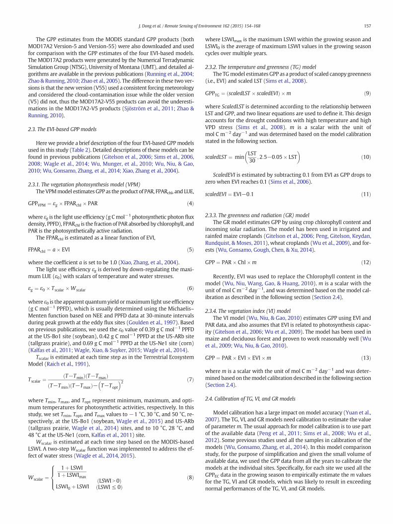
The GPP estimates from the MODIS standard GPP products (bothMOD17A2 Version-5 and Version-55) were also downloaded and usedfor comparison with the GPP estimates of the four EVI-based models.The MOD17A2 products were generated by the Numerical TerradynamicSimulation Group (NTSG), University of Montana (UMT), and detailed al-gorithms are available in the previous publications (Running et al., 2004;Zhao & Running, 2010; Zhao et al., 2005). The difference in these two ver-sions is that the new version (V55) used a consistent forcingmeteorologyand considered the cloud-contamination issue while the older version(V5) did not, thus the MOD17A2-V55 products can avoid the underesti-mations in the MOD17A2-V5 products (Sjöström et al., 2011; Zhao &Running, 2010).

2.3. The EVI-based GPP models

Herewe provide a brief description of the four EVI-based GPPmodelsused in this study (Table 2). Detailed descriptions of these models can befound in previous publications (Gitelson et al., 2006; Sims et al., 2006,2008; Wagle et al., 2014; Wu, Munger, et al., 2010; Wu, Niu, & Gao,2010; Wu, Gonsamo, Zhang, et al., 2014; Xiao, Zhang et al., 2004).

2.3.1. The vegetation photosynthesis model (VPM)TheVPMmodel estimatesGPP as theproduct of PAR, FPARchl, and LUE,

GPPVPM ¼ εg � FPARchl � PAR ð4Þ

where εg is the light use efficiency (g Cmol−1 photosynthetic photon fluxdensity, PPFD), FPARchl is the fraction of PAR absorbed by chlorophyll, andPAR is the photosynthetically active radiation.

The FPARchl is estimated as a linear function of EVI,

FPARchl ¼ a� EVI ð5Þ

where the coefficient a is set to be 1.0 (Xiao, Zhang, et al., 2004).The light use efficiency εg is derived by down-regulating the maxi-

mum LUE (ε0) with scalars of temperature and water stresses.

εg ¼ ε0 � Tscalar �Wscalar ð6Þ

where ε0 is the apparent quantumyield ormaximum light use efficiency(g C mol−1 PPFD), which is usually determined using the Michaelis–Menten function based on NEE and PPFD data at 30-minute intervalsduring peak growth at the eddy flux sites (Goulden et al., 1997). Basedon previous publications, we used the ε0 value of 0.39 g C mol−1 PPFDat the US-Bo1 site (soybean), 0.42 g C mol−1 PPFD at the US-ARb site(tallgrass prairie), and 0.69 g C mol−1 PPFD at the US-Ne1 site (corn)(Kalfas et al., 2011; Wagle, Xiao, & Suyker, 2015; Wagle et al., 2014).

Tscalar is estimated at each time step as in the Terrestrial EcosystemModel (Raich et al., 1991),

Tscalar ¼T−Tminð Þ T−Tmaxð Þ

T−Tminð Þ T−Tmaxð Þ− T−Topt

� �2 ð7Þ

where Tmin, Tmax, and Topt represent minimum, maximum, and opti-mum temperatures for photosynthetic activities, respectively. In thisstudy, we set Tmin, Topt, and Tmax values to −1 °C, 30 °C, and 50 °C, re-spectively, at the US-Bo1 (soybean, Wagle et al., 2015) and US-ARb(tallgrass prairie, Wagle et al., 2014) sites, and to 10 °C, 28 °C, and48 °C at the US-Ne1 (corn, Kalfas et al., 2011) site.

Wscalar is estimated at each time step based on the MODIS-basedLSWI. A two-step Wscalar function was implemented to address the ef-fect of water stress (Wagle et al., 2014, 2015).

Wscalar ¼1þ LSWI

1þ LSWImax

LSWI0 þ LSWILSWI N 0ð ÞLSWI ≤ 0ð Þ

8>><>>:

ð8Þ

where LSWImax is the maximum LSWI within the growing season andLSWI0 is the average of maximum LSWI values in the growing seasoncycles over multiple years.

2.3.2. The temperature and greenness (TG) modelThe TGmodel estimates GPP as a product of scaled canopy greenness

(i.e., EVI) and scaled LST (Sims et al., 2008).

GPPTG ¼ scaledLST � scaledEVIð Þ �m ð9Þ

where ScaledLST is determined according to the relationship betweenLST and GPP, and two linear equations are used to define it. This designaccounts for the drought conditions with high temperature and highVPD stress (Sims et al., 2008). m is a scalar with the unit ofmol C m−2 day−1 and was determined based on the model calibrationstated in the following section.

scaledLST ¼ minLST30

;2:5−0:05� LST� �

ð10Þ

ScaledEVI is estimated by subtracting 0.1 from EVI as GPP drops tozero when EVI reaches 0.1 (Sims et al., 2006).

scaledEVI ¼ EVI−0:1 ð11Þ

2.3.3. The greenness and radiation (GR) modelThe GR model estimates GPP by using crop chlorophyll content and

incoming solar radiation. The model has been used in irrigated andrainfed maize croplands (Gitelson et al., 2006; Peng, Gitelson, Keydan,Rundquist, & Moses, 2011), wheat croplands (Wu et al., 2009), and for-ests (Wu, Gonsamo, Gough, Chen, & Xu, 2014).

GPP ¼ PAR � Chl�m ð12Þ

Recently, EVI was used to replace the Chlorophyll content in themodel (Wu, Niu, Wang, Gao, & Huang, 2010). m is a scalar with theunit of mol C m−2 day−1, and was determined based on the model cal-ibration as described in the following section (Section 2.4).

2.3.4. The vegetation index (VI) modelThe VI model (Wu, Niu, & Gao, 2010) estimates GPP using EVI and

PAR data, and also assumes that EVI is related to photosynthesis capac-ity (Gitelson et al., 2006; Wu et al., 2009). The model has been used inmaize and deciduous forest and proven to work reasonably well (Wuet al., 2009; Wu, Niu, & Gao, 2010).

GPP ¼ PAR � EVI� EVI�m ð13Þ

where m is a scalar with the unit of mol C m−2 day−1 and was deter-mined based on themodel calibration described in the following section(Section 2.4).

2.4. Calibration of TG, VI, and GR models

Model calibration has a large impact on model accuracy (Yuan et al.,2007). The TG, VI, and GRmodels need calibration to estimate the valueof parameterm. The usual approach for model calibration is to use partof the available data (Peng et al., 2011; Sims et al., 2008; Wu et al.,2012). Some previous studies used all the samples in calibration of themodels (Wu, Gonsamo, Zhang, et al., 2014). In this model comparisonstudy, for the purpose of simplification and given the small volume ofavailable data, we used the GPP data from all the years to calibrate themodels at the individual sites. Specifically, for each site we used all theGPPEC data in the growing season to empirically estimate the m valuesfor the TG, VI and GR models, which was likely to result in exceedingnormal performances of the TG, VI, and GR models.

Table 2The model structures and parameters of the four EVI-based models that estimate gross primary production (GPP) of vegetation.

Model PAR FPAR concept FPAR estimation LUE (εg) or environmental down-regulating References

VPM PAR FPARchl f(EVI) ε0 × Tscalar × Wscalar Wagle et al. (2014) and Xiao et al. (2004b)GR PAR FPARchl f(EVI) – Gitelson et al. (2006) and Wu, Gonsamo, Zhang, et al. (2014)TG – FPARgreen f(EVI) f(LST) Sims et al. (2006, 2008)VI PAR FPARgreen f(EVI) f(EVI) Wu, Munger, et al. (2010) and Wu, Niu, and Gao, 2010 (2010)

158 J. Dong et al. / Remote Sensing of Environment 162 (2015) 154–168

In comparison, the VPM model does not need a calibration processfor the flux tower sites used in this study. It uses parameter valuesfrom previous publications, such as maximum LUE parameters (Kalfaset al., 2011; Wagle et al., 2014, 2015). It also uses parameter valuesfrom a standardized parameterization procedure, for example, Tscalarand Wscalar in the model.

Fig. 2. Seasonal dynamics and interannual variations of air temperature, precipitation, photosydays at the three flux tower sites (a. US-Bo1, b. US-Ne1, and c. US-ARb).

2.5. Evaluation of model performance

The predictedGPPs from the fourmodels (GPPVPM, GPPTG, GPPVI, andGPPGR) were evaluated against the GPPEC. First, the seasonal dynamicsof the simulated GPPswere compared. Second, the Pearson's correlationcoefficient (r) and the root mean squared error (RMSE) were calculated

nthetically active radiation (PAR), and vapor pressure deficit (VPD) with an interval of 8-

Fig. 3. Seasonal dynamics and interannual variations of gross primary production (GPPEC) (a. USNDVI (d. US-Bo1, e. US-Ne1, and f. US-ARb), EVI (g. US-Bo1, h. US-Ne1, and i. US-ARb), and LSW

Table 3Meteorological statistics in the growing seasons of different site–years to identifydroughts.

Site ID Years VPDmean

(hPa)Precipitation(mm)

Ta_fmean

(°C)Rg_fmean

(MJ m−2 day−1)

US-Bo1 2002a 8.49 153 23.54 22.372004 5.48 367 20.96 22.682006 5.86 362 22.15 19.41Average 6.61 294 22.22 21.49

US-Ne1 2007 7.53 605 22.49 20.722008 7.83 690 21.02 20.422009 7.56 457 20.56 20.942010 6.78 634 22.82 22.382011 7.22 515 20.92 20.992012a 12.01 514 23.16 24.84Average 8.12 569 21.76 21.64

US-ARb 2005 8.99 546 22.27 19.412006a 13.42 432 23.47 20.16Average 11.16 489 22.86 19.78

a Drought years.

159J. Dong et al. / Remote Sensing of Environment 162 (2015) 154–168

to quantify the agreement between GPPEC and predicted GPPs duringthe plant growing season. In addition, the linear regression model wasused to determine the relationship between predicted GPPs andGPPEC, and the coefficient of determination (R2) was used to evaluatethemodels' explanatory abilities for GPP variances. Third, the seasonallyintegrated GPPs can quantify biases of the modeled GPPs in magnitude.

3. Results

3.1. Comparison of climate, GPP, and vegetation indices in drought andnon-drought years

We identified site–years that experienced severe droughts duringthe plant growing season based on meteorological data. Following thesame definition as in previous works (Jin et al., 2013; Kalfas et al.,2011; Wagle et al., 2014), the plant growing season was definedas the period of GPP N 1 g C m−2 day−1. The US-Bo1, US-Ne1, and US-

-Bo1, b. US-Ne1, and c. US-ARb) and vegetation indices at the three CO2 flux sites, includingI(j. US-Bo1, k. US-Ne1, and l. US-ARb).

Fig. 4. The relationships between gross primary production (GPPEC) and vegetation indices (NDVI and EVI) in the drought years (a. US-Bo1 2004, 2006; c. US-Ne1 2007–2011; and e. US-ARb 2005) and non-drought years (b. US-Bo1 2002, d. US-Ne1 2012, and f. US-ARb 2006) at the three CO2 flux tower sties.

160 J. Dong et al. / Remote Sensing of Environment 162 (2015) 154–168

ARb sites showed drought signals in 2002, 2012, and 2006, respectively,as indicated by VPD (Fig. 2, Table 3). The US-Bo1 site had an averageVPD of 8.49 hPa in the 2002 growing season, much higher than in2004 (5.48 hPa) and 2006 (5.86 hPa). Also, its precipitation in the2002 growing season was 153 mm, which was at least 50% lower thanother years (367 mm in 2004 and 362 mm in 2006, Table 3). The US-Ne1 site experienced drought in 2012 with a high VPD of 12.01 hPawhile the average VPD in 2007–2011 was only 7.40 hPa (Table 3). Atthe US-ARb site, the VPD in the 2006 growing season was 49% higherthan in 2005, also the precipitation in 2006 was 21% less than in 2005.All three sites also had higher air temperature and radiation in thedrought years than in non-drought years (Fig. 2).

Observed carbon fluxes and satellite-based vegetation indicesdropped significantly in those drought years, i.e., 2002 at US-Bo1,2012 at US-Ne1 and 2006 at US-ARb (Fig. 3). At the US-Bo1 site, the av-erage GPPEC of soybean in the 2002 growing season decreased by 40%relative to the non-drought years (2004 and 2006), while NDVI, EVIand LSWI decreased by 9%, 19%, and 55%, respectively. The same phe-nomenon also happened at the US-ARb site; the average GPPEC of grass-land in the 2006 growing season decreased by 49% compared to those ofthe non-drought years (2005), while NDVI, EVI, and LSWI decreased by21%, 22%, and 111%, respectively. At the irrigated US-Ne1 site, GPPECdropped significantly in August, as did NDVI, EVI and LSWI (Fig. 3).

3.2. The relationships between vegetation indices (NDVI and EVI) andGPPECin drought and non-drought years

We regrouped all data into (1) non-drought years and (2) droughtyears for each site, and carried out simple linear regression analysis ofGPPEC and vegetation indices (NDVI and EVI). For the non-droughtsite-years, EVI accounted for more variance of GPP (with higher coeffi-cient of determination) than did NDVI (Fig. 4a, c, and e). For example,at the US-Bo1 site in 2004 and 2006, the EVI and NDVI accounted for75% and 67% of GPP variances, respectively. For the drought site–years, EVI also accounted for more GPP variance than did NDVI. At theUS-Bo1 site in 2002, the EVI and NDVI accounted for 78% and 73% ofGPP variances, respectively (Fig. 4b). At the US-ARb site in 2006, EVIand NDVI explained 75% and 53% of GPP variances (Fig. 4f). At the US-Ne1 site in 2012, EVI and NDVI accounted similarly for GPP variances,at 86% and 90%, respectively (Fig. 4d). In general, EVI better explainedGPP variances than did NDVI under both non-drought and droughtconditions.

For comparison between the drought and non-drought site–years,the results showed that the linear relationship between vegetation indi-ces (EVI and NDVI) and GPPEC was slightly stronger during the droughtsite–years (Fig. 4b, d, and f) than the non-drought site–years (Fig. 4a, c,and e). This demonstrated that the sensitivity of EVI and NDVI to GPP

161J. Dong et al. / Remote Sensing of Environment 162 (2015) 154–168

could be higher under drought (water stress) than non-drought condi-tions. However, to confirm this result, additional data analysis indrought and non-drought years is still needed in the future.

3.3. Comparison of GPP estimates from the models (VPM, TG, GR, and VI)and flux towers in drought and non-drought years

3.3.1. Seasonal dynamics of GPP estimates from models and towersFig. 5 shows that the seasonal dynamics of GPP estimates from the

four EVI-based models tracked GPPEC reasonably well during droughtand non-drought years at all three study sites, despite the differencein growing season lengths and water management (irrigation andrainfed). The growing season of soybean at the US-Bo1 site starts be-tween May 16 and June 2 and ends between September 5 and 14(Table 4). Corn crops at the US-Ne1 site had similar starting dates buta longer growing season that lasted till early October. Grassland in theUS-ARb site had the longest growing season, from early April to mid-October (Fig. 3). As drought occurred on different dates and lasted forvarious lengths of time, the effects of drought on seasonal dynamics ofGPP and vegetation indices were different at each site. At the US-Bo1site (2002), drought first occurred in late June and lasted until lateJuly. At the US-Ne1 site, drought began in late July and lasted untilearly September. The drought at theUS-Ne1 site led to an earlier harvestof corn crops in 2012 in comparison to other years (2007–2011). Thedrought at theUS-ARb site (2006) started from early June to September.In general, all four models captured the seasonal dynamics very well innon-drought years and fairly well in drought years.

Fig. 5. A comparison on seasonal dynamics of gross primary production from the flux tower sdrought year (a. US-Bo12004; c. US-Ne12011, and e. US-ARb2005) and a non-drought year (b. Uthe visualization, only one year of data from non-drought years was used to showcase intra-an

Besides the starting and end dates of the growing season, we alsocompared the emergence dates when the maximum GPP appeared(Table 4). RMSEs of GPPEC and GPPVPM aswell as GPPTG had a lowest de-viation of 15 days while GPPVI and GPPGR had a larger deviation withGPPEC (18 days). This indicated that VPMand TGmodels performed bet-ter in simulating the dates when GPP reached maximum.

3.3.2. Correlation analysis of GPP estimates from models and towersIn terms of the individual sites, the linear regression analysis indicat-

ed that in non-drought years all fourmodels had generally good explan-atory capabilities for GPP variance at the three sites (VPM: RMSE1.87 ~ 2.27, R2 N 0.95; TG: RMSE 2.58 ~ 3.35, R2 N 0.91, VI: RMSE1.84 ~ 2.68, R2 N 0.96, and GR: RMSE 2.05 ~ 3.24, R2 N 0.95, Fig. 6).RMSE of GPPEC and GPPVPM was lowest for most site–years among thefourmodels (Table 5). The performance of themodels in drought condi-tions was also evaluated at the individual sites (US-Bo1 2002, US-Ne12012, andUS-ARb 2006) (Fig. 7). Results show that the fourmodels per-formed differently. The VPM model had the lowest RMSE (0.99 ~ 2.39)and highest explanatory capability for GPP variance with R2 of 0.96–0.98. GPPVI also had a significant relationship with observed GPP at allthree sites but with a higher RMSE (1.39 ~ 3.24) and lower explanatorycapability (with R2 of 0.94, 0.97, and 0.93 at US-Bo1, US-Ne1, and US-ARb respectively). The TG (with R2 0.74–0.91) and GR models (withR2 0.85–0.96) had weaker explanatory capabilities for GPP variancesthan the other two models during the drought years (Fig. 7). RMSEand R2 analysis of GPPEC and estimated GPP from the four modelsshowed that VPM-based results were the most consistent with GPPECand explained the GPP variances most (Table 5).

ites (GPPEC) and the four EVI-based models (GPPVPM, GPPVPM, GPPVPM, and GPPVPM) in aS-Bo1 2002; d. US-Ne12012; and f. US-ARb 2006) at the three flux tower sites. To enhancenual variation of GPPs.

Fig. 6. The relationships between gross primary production from the CO2 flux tower sites (Gthe non-drought years at the three flux tower sites: The VPM (a. US-Bo1, b. US-Ne1, and c. Uh. US-Ne1, and i. US-ARb), and the GR model (j. US-Bo1, k. US-Ne1, and l. US-ARb).

Table 4The root mean squared errors (RMSEs) between the dates of maximum GPPEC andmodeled GPPs for the three study sites. The growing season is defined as the period withGPP N 1 g C m−2 day−1.

Site Year Growing season GPPEC GPPVPM GPPTG GPPVI GPPGR

US-Bo1 2002a 5/25–9/14 7/28 8/5 7/28 8/5 8/52004 5/16–9/5 7/11 8/4 7/19 8/4 8/42006 6/2–9/14 7/28 7/28 7/12 8/21 8/21

US-Ne1 2007 5/25–9/22 7/4 7/12 7/28 7/28 7/282008 6/1–10/7 7/11 7/27 7/27 7/27 7/272009 5/17–9/22 7/12 7/4 7/28 7/28 7/282010 5/25–9/6 7/20 7/12 8/5 7/28 7/282011 6/2–10/8 7/12 7/20 7/20 7/20 7/202012a 5/16–9/5 6/25 7/11 6/17 6/25 6/17

US-ARb 2005 4/7–10/16 6/18 7/20 7/4 7/20 7/202006a 4/15–10/16 6/2 6/2 6/18 6/18 6/2

RMSEs of peak GPP dates 15d 15d 18d 18d

a Drought years.

162 J. Dong et al. / Remote Sensing of Environment 162 (2015) 154–168

In terms of all the non-drought site–years, Fig. 8 shows that simulat-ed GPP from all four models (GPPVPM, GPPTG, GPPVI and GPPGR) had rea-sonably good agreementwith GPPEC (R2 N 0.95). That being said, in eachdrought site–year, the four models had different performances. TheGPPVPM was significantly correlated with GPPEC (R2 = 0.97, Fig. 8).The VI model also had a significant relationship with GPPEC but withslightly lower explanatory capability (R2 = 0.94), while TG and GRmodels had lower explanation of GPPEC variances (TG, R2 = 0.84; GR,R2 = 0.91) in terms of all the drought site–years (Fig. 8). RMSE ofGPPEC and GPPVPM was the lowest (1.61 g C m−2 day−1) compared toother models (TG 3.90, VI 2.32, and GR 3.16 g C m−2 day−1).

3.3.3. Comparison of annual (seasonal) sum of GPP estimates from modelsand towers

The seasonally integrated GPP analysis indicated that in the non-drought site–years GPP estimates from all four models were reasonably

PPEC) and predicted GPPs from the four models (GPPVPM, GPPTG, GPPVI, and GPPGR) inS-ARb), the TGmodel (d. US-Bo1, e. US-Ne1, and f. US-ARb), the VI model (g. US-Bo1,

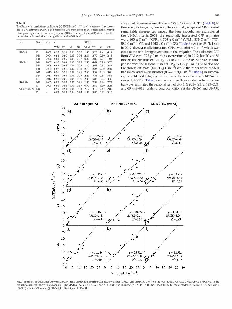
Fig. 7. The linear relationships between gross primary production from the CO2 flux tower sitesdrought years at the three flux tower sites: The VPM (a. US-Bo1, b. US-Ne1, and c. US-ARb), theUS-ARb), and the GR model (j. US-Bo1, k. US-Ne1, and l. US-ARb).

Table 5The Pearson's correlation coefficients (r), RMSEs (g C m−2 day−1) between flux tower-based GPP estimates (GPPEC) and predicted GPP from the four EVI-based models withinplant growing season in non-drought years (ND) and drought years (D) at the three fluxtower sites. All correlations are significant at the 0.01 level.

Site Status Year r RMSE

VPM TG VI GR VPM TG VI GR

US-Bo1 D 2002 0.95 0.91 0.91 0.82 1.43 3.23 2.41 4.14ND 2004 0.94 0.90 0.93 0.96 2.81 2.70 2.60 2.15ND 2006 0.98 0.95 0.94 0.97 0.93 2.86 2.01 1.94

US-Ne1 ND 2007 0.96 0.84 0.93 0.95 2.40 4.61 3.25 3.70ND 2008 0.97 0.96 0.96 0.95 1.87 2.63 2.54 2.83ND 2009 0.97 0.97 0.97 0.98 2.13 2.24 2.89 2.33ND 2010 0.96 0.95 0.98 0.95 2.55 3.52 1.83 3.66ND 2011 0.96 0.95 0.96 0.97 2.41 3.35 2.58 3.58D 2012 0.96 0.80 0.95 0.96 2.39 5.85 3.24 3.30

US-ARb ND 2005 0.89 0.84 0.90 0.91 1.87 2.58 1.84 2.23D 2006 0.96 0.51 0.90 0.87 0.99 2.52 1.39 2.23

All site-years ND – 0.95 0.91 0.94 0.93 2.17 3.10 2.47 2.85D – 0.97 0.83 0.94 0.94 1.61 3.90 2.32 3.16

163J. Dong et al. / Remote Sensing of Environment 162 (2015) 154–168

consistent (deviation ranged from−17% to 17%)withGPPEC (Table 6). Inthe drought site–years, however, the seasonally integrated GPP showedremarkable divergences among the four models. For example, atthe US-Bo1 site in 2002, the seasonally integrated GPP estimateswere 660 g C m−2 (GPPEC), 706 g C m−2 (VPM), 839 C m−2 (TG),982 C m−2 (VI), and 1062 g C m−2 (GR) (Table 6). At the US-Ne1 sitein 2012, the seasonally integrated GPPEC was 1661 g C m−2, which wasclose to the non-drought year due to the irrigation. The estimated GPPfrom VPM was 1725 g C m−2 (4% overestimate) in 2012, but TG and VImodels underestimated GPP by 12% to 20%. At the US-ARb site, in com-parison with the seasonal sum of GPPEC (733.6 g C m−2), VPM also hadthe closest estimate (816.96 g C m−2) while the other three modelshadmuch larger overestimates (867–1059 g Cm−2, Table 6). In summa-ry, the VPMmodel slightly overestimated the seasonal sum of GPP in therange of 4%–11% (Table 6), while the other three models either substan-tially overestimated the seasonal sum of GPP (TG 20%–49%, VI 18%–27%,and GR 44%–61%) under drought conditions at the US-Bo1 and US-ARb

(GPPEC) and predicted GPP from the fourmodels (GPPVPM, GPPTG, GPPVI, and GPPGR) in theTGmodel (d. US-Bo1, e. US-Ne1, and f. US-ARb), the VI model (g. US-Bo1, h. US-Ne1, and i.

Fig. 8. The relationships between gross primary production from the CO2 flux tower sites (GPPEC) and predicted GPP from the four models in all non-drought site–years (a. GPPVPM, b.GPPTG, c. GPPVI, and d. GPPGR) and in all drought site–years (e. GPPVPM, f. GPPTG, g. GPPVI, and h. GPPGR).

164 J. Dong et al. / Remote Sensing of Environment 162 (2015) 154–168

sites or underestimated GPP (TG−20%, VI−12%) under drought condi-tions at the irrigated US-Ne1 site.

4. Discussion

4.1. Performance of EVI/FPARchl- and EVI/FPARgreen-based GPP models incomparison to NDVI/FPARcanopy-based GPP models

The results from this study have shown that the predicted GPP fromthe four EVI-based models have good agreement with the GPPEC atmaize, soybean, and tallgrass prairie sites in non-drought conditions.This could be partly attributed to the application of the chlorophyll orgreen leaves-based theory and the use of chlorophyll-related vegetationindices (i.e., EVI) (Gitelson et al., 2014; Rossini et al., 2014). Previousstudy presented that EVI-based FPARchl exhibited seasonal dynamicsmore similar with GPPEC than did FPARcanopy from NDVI (likeMOD15A2 products) (Cheng, Zhang, Lyapustin, Wang, & Middleton,2014). In these models, EVI was used to estimate FPARchl, FPARgreen

and GPP. This study once again showed that the EVI has a stronger rela-tionshipwith GPP thandoes NDVI in soybean,maize, and grassland eco-systems (Fig. 4), which is consistent with previous studies inagricultural, grassland, and forest ecosystems (Jin et al., 2013; Kalfaset al., 2011; Peng, Gitelson, & Sakamoto, 2013; Wagle et al., 2014; Wu,Niu, & Gao, 2010; Xiao, Hollinger, et al., 2004; Xiao, Zhang, et al., 2004;Xiao et al., 2005; Zhang et al., 2006).

Table 6The sums of gross primary productionwithin the plant growing season (GPP, g Cm−2) in non-drepresents the period with GPP N 1 g C m−2 day−1. The percentage numbers inside the bracke

Site Status Year Growing season GPPEC

US-Bo1 D 2002 5/25–9/14 660ND 2004 5/16–9/5 1198ND 2006 6/2–9/14 948

US-Ne1 ND 2007 5/25–9/22 1811ND 2008 6/1–10/7 1743ND 2009 5/17–9/22 1916ND 2010 5/25–9/6 1620ND 2011 6/2–10/8 1637D 2012 5/16–9/5 1661

US-ARb ND 2005 4/7–10/16 1513D 2006 4/15–10/16 734

This study focused on the inter-comparison of EVI-basedmodels, in-stead of the comparison between EVI- and NDVI-based models, as pre-vious studies have already done so (Sims et al., 2008; Sjöström et al.,2011; Wu et al., 2011). For example, the comparison of GR model andPSN model at individual sites showed that the GR model performs bet-ter in terms ofmodel accuracy and stability (Wu, Gonsamo, Zhang, et al.,2014). In addition, VPM, TG, and VI models providedmore reliable esti-mates of GPP than that of standard MODIS GPP products (MOD17A2),and VPM tracked well the seasonal dynamics of GPP in forests (Wu,Munger, et al., 2010). Several studies have also reported that the stan-dard MODIS GPP products did not accurately estimate carbon uptakeduring drought conditions (Hwang et al., 2008; Nightingale, Coops,Waring, & Hargrove, 2007; Zhang et al., 2007). Here, we analyzed theGPP estimates from both MOD17A2 Version-5 and Version-55 for thethree flux tower sites in this study (Fig. 9). The MOD17A2 productsshowed higher explanation of GPP variances in the non-drought yearsthan in drought years; however, both versions of MOD17A2 productssignificantly underestimated GPP in both drought and non-droughtyears (Fig. 9).

4.2. The model structures and their sensitivities to water stress indrought years

While all the four EVI-based models in this study had good perfor-mance in the non-drought years, these models differed substantiallyin drought years, reflecting differences in the model design or

rought years (ND) and drought years (D) at the three flux tower sites. The growing seasonts mean the overestimate or underestimate rates relative to the GPPEC.

GPPVPM GPPTG GPPVI GPPGR

706 (7%) 982 (49%) 839 (27%) 1062 (61%)996 (−17%) 1146 (−4%) 1241 (4%) 1289 (8%)906 (−4%) 1235 (30%) 1072 (13%) 1108 (17%)

1844 (2%) 1898 (5%) 1673 (−8%) 1818 (0%)1697 (−3%) 1849 (6%) 1548 (−11%) 1778 (2%)2015 (5%) 2097 (9%) 2096 (9%) 2070 (8%)1770 (9%) 1774 (10%) 1622 (0%) 1757 (8%)1644 (0%) 1763 (8%) 1538 (−6%) 1787 (9%)1725 (4%) 1336 (−20%) 1457 (−12%) 1772 (7%)1482 (−2%) 1490 (−2%) 1429 (−6%) 1360 (−10%)817 (11%) 878 (20%) 866 (18%) 1059 (44%)

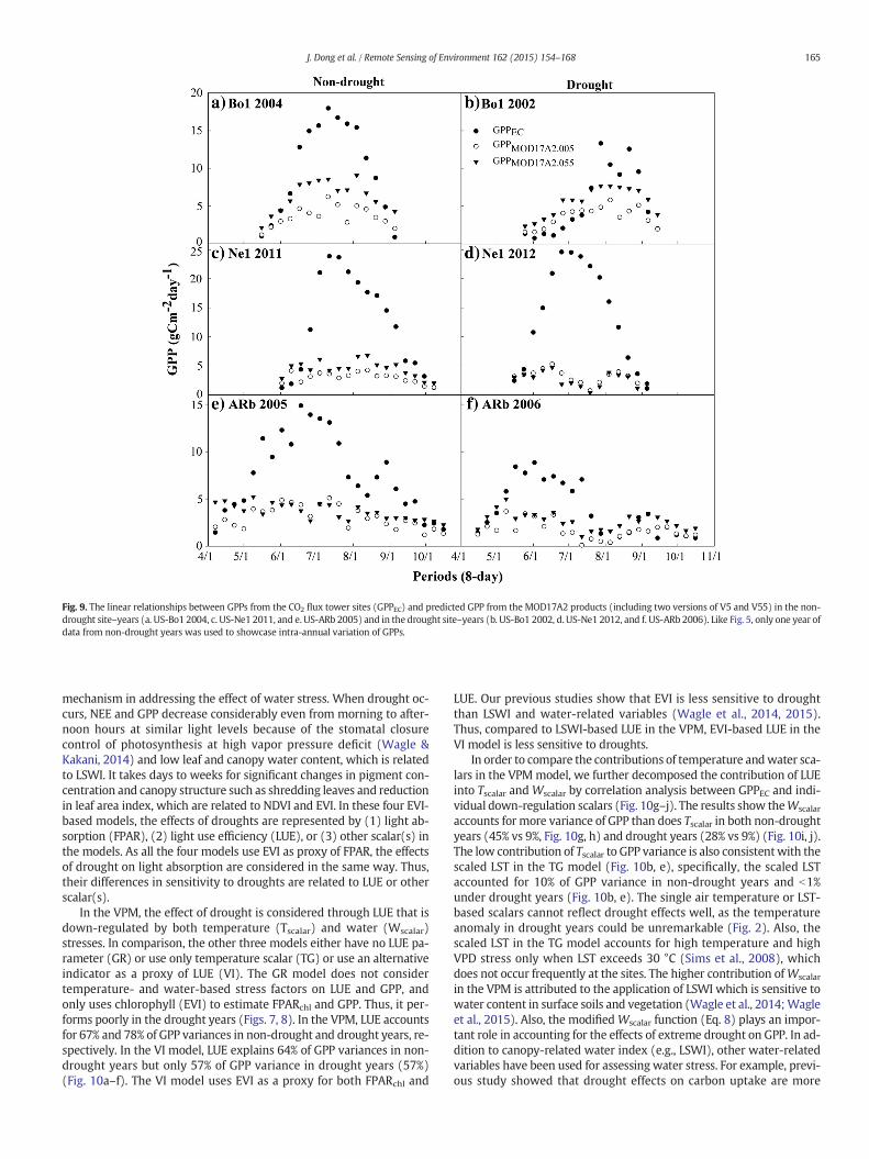
Fig. 9. The linear relationships between GPPs from the CO2 flux tower sites (GPPEC) and predicted GPP from the MOD17A2 products (including two versions of V5 and V55) in the non-drought site–years (a. US-Bo1 2004, c. US-Ne1 2011, and e. US-ARb 2005) and in the drought site–years (b. US-Bo1 2002, d. US-Ne1 2012, and f. US-ARb 2006). Like Fig. 5, only one year ofdata from non-drought years was used to showcase intra-annual variation of GPPs.

165J. Dong et al. / Remote Sensing of Environment 162 (2015) 154–168

mechanism in addressing the effect of water stress. When drought oc-curs, NEE and GPP decrease considerably even from morning to after-noon hours at similar light levels because of the stomatal closurecontrol of photosynthesis at high vapor pressure deficit (Wagle &Kakani, 2014) and low leaf and canopy water content, which is relatedto LSWI. It takes days to weeks for significant changes in pigment con-centration and canopy structure such as shredding leaves and reductionin leaf area index, which are related to NDVI and EVI. In these four EVI-based models, the effects of droughts are represented by (1) light ab-sorption (FPAR), (2) light use efficiency (LUE), or (3) other scalar(s) inthe models. As all the four models use EVI as proxy of FPAR, the effectsof drought on light absorption are considered in the same way. Thus,their differences in sensitivity to droughts are related to LUE or otherscalar(s).

In the VPM, the effect of drought is considered through LUE that isdown-regulated by both temperature (Tscalar) and water (Wscalar)stresses. In comparison, the other three models either have no LUE pa-rameter (GR) or use only temperature scalar (TG) or use an alternativeindicator as a proxy of LUE (VI). The GR model does not considertemperature- and water-based stress factors on LUE and GPP, andonly uses chlorophyll (EVI) to estimate FPARchl and GPP. Thus, it per-forms poorly in the drought years (Figs. 7, 8). In the VPM, LUE accountsfor 67% and 78% of GPP variances in non-drought and drought years, re-spectively. In the VI model, LUE explains 64% of GPP variances in non-drought years but only 57% of GPP variance in drought years (57%)(Fig. 10a–f). The VI model uses EVI as a proxy for both FPARchl and

LUE. Our previous studies show that EVI is less sensitive to droughtthan LSWI and water-related variables (Wagle et al., 2014, 2015).Thus, compared to LSWI-based LUE in the VPM, EVI-based LUE in theVI model is less sensitive to droughts.

In order to compare the contributions of temperature andwater sca-lars in the VPMmodel, we further decomposed the contribution of LUEinto Tscalar and Wscalar by correlation analysis between GPPEC and indi-vidual down-regulation scalars (Fig. 10g–j). The results show theWscalar

accounts for more variance of GPP than does Tscalar in both non-droughtyears (45% vs 9%, Fig. 10g, h) and drought years (28% vs 9%) (Fig. 10i, j).The low contribution of Tscalar to GPP variance is also consistentwith thescaled LST in the TG model (Fig. 10b, e), specifically, the scaled LSTaccounted for 10% of GPP variance in non-drought years and b1%under drought years (Fig. 10b, e). The single air temperature or LST-based scalars cannot reflect drought effects well, as the temperatureanomaly in drought years could be unremarkable (Fig. 2). Also, thescaled LST in the TG model accounts for high temperature and highVPD stress only when LST exceeds 30 °C (Sims et al., 2008), whichdoes not occur frequently at the sites. The higher contribution ofWscalar

in the VPM is attributed to the application of LSWI which is sensitive towater content in surface soils and vegetation (Wagle et al., 2014;Wagleet al., 2015). Also, the modified Wscalar function (Eq. 8) plays an impor-tant role in accounting for the effects of extreme drought on GPP. In ad-dition to canopy-related water index (e.g., LSWI), other water-relatedvariables have been used for assessing water stress. For example, previ-ous study showed that drought effects on carbon uptake are more

Fig. 10. The effects of light use efficiency (LUE) or environmental limitation factors of the EVI-based models on GPP in both non-drought (a. VPM, b. TG, and c. VI) and drought years(d. VPM, e. TG, and f. VI). The GR model was not included here as it does not have the LUE factor. The correlations of GPPEC vs Tscalar and GPPEC vs Wscalar are shown in g) andh) respectively for non-drought years, and i) and j) respectively for drought years.

166 J. Dong et al. / Remote Sensing of Environment 162 (2015) 154–168

closely related to soil water stress rather than atmospheric controls(temperature and VPD) (Hwang et al., 2008). However, due to spatialheterogeneity, no soil water content data are available for an ecosystemscale application.

4.3. Trade-off between comprehensiveness and applicability in satellite-basedGPP models

All the four models have similar parameterization in FPAR, thoughthe LUE estimates are different. Compared to the TG, VI, and GRmodels,the more sophisticated LUE structure of VPM could be the primary rea-son for its better performance in GPP simulations under various climateconditions. However, more parameters mean more requirements fordata inputs. While the VPM can simulate GPP more accurately, TG, VIand GR models can be applied to the places without meteorologicaldata. Model selection requires considering the ecosystem types, envi-ronmental stress status, and data availability. This study suggests thatin drought areas or under drought conditions, the VPM model is a bestchoice among the four models. The VI model is an alternative optionwhen no meteorological data are available. The TG and GR models canbe used in the areas without water stress like irrigated croplands.

Another concern is model calibration, as the TG, VI, and GR modelsrequire calibration before application, which requires in-situ data forempirical statistical analysis. In this study, we used all the in-situ datafor the model calibration (TG, VI, and GR) due to less data availability,

which is not an ideal approach and can induce bias of model perfor-mance. Therefore, the actual performance of the three models couldbe different than what we reported here. In comparison, the VPMmodel only needs calibration for themaximumLUE or it can be acquiredfrom existing publications; it is therefore more suitable to upscale sim-ulations at various spatial and temporal domains. Satellite-derived PARdata fromhigh spatial resolution GLASS images have been proven effec-tive in GPP simulations (Cai et al., 2014), and the VPM model can alsouse LST data to replace air temperature data, which can help to reducethe dependence of the model on meteorological measurements andmake VPM an independent, satellite-driven, and more operationalmodel.

While VPM uses LSWI to determine the effect of water stress, somestudies used other ancillary data or variables like LST, actual and poten-tial evapotranspiration (AET and PET) to improve the LUE parameter(Maselli, Papale, Puletti, Chirici, & Corona, 2009; Moreno et al., 2012;Yang, Shang, Guan, & Jiang, 2013). The use of LSWI is convenient asthe data are available from MODIS and Landsat. All the comparisonsconducted in this study are based on the limited flux towers of cropsand grasslands, and both plant types are herbaceous which havelower tolerance capability to drought, compared to woody forests(Baldocchi, Xu, & Kiang, 2004). Therefore, further evaluation of LSWIperformance in drought conditions and its improvement of the water-related downscaling regulation parameter (Wscalar) are still needed forother ecosystem types (e.g., forest) in the future study.

167J. Dong et al. / Remote Sensing of Environment 162 (2015) 154–168

5. Conclusions

In this study,we investigated and evaluated the performance and ro-bustness of four widely used EVI-based GPP models (VPM, TG, VI, andGR) under drought conditions by using observation data from threeAmeriFlux sites (soybean, grassland, and maize). Correlation analysisbetween GPPEC and vegetation indices (NDVI and EVI) indicated thatEVI and NDVI accounted for more GPP variance in drought conditionsthan in non-drought conditions. Furthermore, EVI accounted for moreGPP variance than did NDVI in drought conditions. All the GPP estimatesfrom the fourmodels had generally good agreementwith GPP estimates(GPPEC) from theflux towers in non-drought conditions. However, theirperformances varied in drought conditions, and VPM was more robustduring drought years than the VI, TG, and GR models. This discrepancycould be related to the inclusion of a water stress scalar in VPM basedon LSWI, whereas the other three models either do not have a directwater stress scalar (GR model) or use substitutive variables (TG and VImodels). This study implies that water stress regulation on light use ef-ficiency and GPP should be considered in these models applied underdrought conditions in order to estimate terrestrial carbon fluxes in thecontext of global climate change aswell as increasing climate variabilityand extreme events. However, more investigations are needed to ex-plore the possible different sensitivities of the models in the otherplant function types (e.g., forests).

Acknowledgments

This study was supported in part by a research grant (Project No.2012-02355) through the USDANational Institute for Food and Agricul-ture (NIFA)'s Agriculture and Food Research Initiative (AFRI), RegionalApproaches for Adaptation to and Mitigation of Climate Variability andChange, and a research grant from the National Science FoundationEPSCoR (IIA-1301789). The studied AmeriFlux sites were supported bythe U.S. Department of Energy (DOE), Office of Science, Office of Biolog-ical and Environmental Research (Grants No. DE-AC02-05CH11231, DE-FG03-00ER62996, DE-FG02-03ER63639, and DE-EE0003149), DOE-EPSCoR (Grant No. DE-FG02-00ER45827), and NASA NACP (Grant No.NNX08AI75G). We thank Drs. Qingyuan Zhang, Jianyang Xia, Mr. YaoZhang and two anonymous reviewers for their comments and sugges-tions on the previous version of the manuscript.

References

Agarwal, D. A., Humphrey, M., Beekwilder, N. F., Jackson, K. R., Goode, M. M., & van Ingen,C. (2010). A data-centered collaboration portal to support global carbon-flux analysis.Concurrency and Computation: Practice and Experience, 22, 2323–2334.

Asaf, D., Rotenberg, E., Tatarinov, F., Dicken, U., Montzka, S. A., & Yakir, D. (2013). Ecosys-tem photosynthesis inferred from measurements of carbonyl sulphide flux. NatureGeoscience, 6, 186–190.

Baldocchi, D. (2014). Measuring fluxes of trace gases and energy between ecosystems andthe atmosphere—The state and future of the eddy covariance method. Global ChangeBiology, 20, 3600–3609.

Baldocchi, D. D., Xu, L. K., & Kiang, N. (2004). How plant functional-type, weather, season-al drought, and soil physical properties alter water and energy fluxes of an oak-grasssavanna and an annual grassland. Agricultural and Forest Meteorology, 123, 13–39.

Barman, R., Jain, A. K., & Liang, M. L. (2014). Climate-driven uncertainties in modeling ter-restrial gross primary production: A site level to global-scale analysis. Global ChangeBiology, 20, 1394–1411.

Beer, C., Reichstein, M., Tomelleri, E., Ciais, P., Jung, M., Carvalhais, N., et al. (2010). Terres-trial gross carbon dioxide uptake: Global distribution and covariation with climate.Science, 329, 834–838.

Cai, W. W., Yuan, W. P., Liang, S. L., Zhang, X. T., Dong, W. J., Xia, J. Z., et al. (2014). Im-proved estimations of gross primary production using satellite-derived photosyn-thetically active radiation. Journal of Geophysical Research — Biogeosciences, 119,110–123.

Cheng, Y. B., Zhang, Q. Y., Lyapustin, A. I., Wang, Y. J., & Middleton, E. M. (2014). Impacts oflight use efficiency and fPAR parameterization on gross primary production model-ing. Agricultural and Forest Meteorology, 189, 187–197.

Desai, A. R., Richardson, A. D., Moffat, A. M., Kattge, J., Hollinger, D. Y., Barr, A., et al. (2008).Cross-site evaluation of eddy covariance GPP and RE decomposition techniques.Agricultural and Forest Meteorology, 148, 821–838.

Fischer, M. L., Torn, M. S., Billesbach, D. P., Doyle, G., Northup, B., & Biraud, S. C. (2012).Carbon, water, and heat flux responses to experimental burning and drought in atallgrass prairie. Agricultural and Forest Meteorology, 166, 169–174.

Gitelson, A. A., Peng, Y., Arkebauer, T. J., & Schepers, J. (2014). Relationships between grossprimary production, green LAI, and canopy chlorophyll content inmaize: Implicationsfor remote sensing of primary production. Remote Sensing of Environment, 144, 65–72.

Gitelson, A. A., Vina, A., Ciganda, V., Rundquist, D. C., & Arkebauer, T. J. (2005). Remote es-timation of canopy chlorophyll content in crops. Geophysical Research Letters, 32.

Gitelson, A. A., Vina, A., Verma, S. B., Rundquist, D. C., Arkebauer, T. J., Keydan, G., et al.(2006). Relationship between gross primary production and chlorophyll content incrops: Implications for the synoptic monitoring of vegetation productivity. Journalof Geophysical Research-Atmospheres, 111.

Goulden, M. L., Daube, B. C., Fan, S. M., Sutton, D. J., Bazzaz, A., Munger, J. W., et al. (1997).Physiological responses of a black spruce forest to weather. Journal of GeophysicalResearch-Atmospheres, 102, 28987–28996.

Huete, A., Didan, K., Miura, T., Rodriguez, E. P., Gao, X., & Ferreira, L. G. (2002). Overview ofthe radiometric and biophysical performance of the MODIS vegetation indices.Remote Sensing of Environment, 83, 195–213.

Huete, A. R., Liu, H. Q., Batchily, K., & vanLeeuwen, W. (1997). A comparison of vegetationindices over a global set of TM images for EOS-MODIS. Remote Sensing of Environment,59, 440–451.

Hwang, T., Kangw, S., Kim, J., Kim, Y., Lee, D., & Band, L. (2008). Evaluating drought effecton MODIS gross primary production (GPP) with an eco-hydrological model in themountainous forest, East Asia. Global Change Biology, 14, 1037–1056.

Jin, C., Xiao, X. M., Merbold, L., Arneth, A., Veenendaal, E., & Kutsch, W. L. (2013). Phenol-ogy and gross primary production of two dominant savannawoodland ecosystems inSouthern Africa. Remote Sensing of Environment, 135, 189–201.

Kalfas, J. L., Xiao, X., Vanegas, D. X., Verma, S. B., & Suyker, A. E. (2011). Modeling gross pri-mary production of irrigated and rain-fed maize using MODIS imagery and CO2 fluxtower data. Agricultural and Forest Meteorology, 151, 1514–1528.

Maselli, F., Papale, D., Puletti, N., Chirici, G., & Corona, P. (2009). Combining remote sens-ing and ancillary data to monitor the gross productivity of water-limited forest eco-systems. Remote Sensing of Environment, 113, 657–667.

Meijering, E. (2002). A chronology of interpolation: From ancient astronomy to modernsignal and image processing. Proceedings of the IEEE, 90, 319–342.

Meyers, T. P., & Hollinger, S. E. (2004). An assessment of storage terms in the surface en-ergy balance ofmaize and soybean. Agricultural and Forest Meteorology, 125, 105–115.

Monteith, J. L. (1972). Solar radiation and productivity in tropical ecosystems. Journal ofApplied Ecology, 9, 747–766.

Monteith, J. L. (1977). Climate and efficiency of crop production in Britain. PhilosophicalTransactions of the Royal Society of London. Series B: Biological Sciences, 281, 277–294.

Moreno, A., Maselli, F., Gilabert, M. A., Chiesi, M., Martinez, B., & Seufert, G. (2012). Assess-ment ofMODIS imagery to track light-use efficiency in awater-limitedMediterraneanpine forest. Remote Sensing of Environment, 123, 359–367.

Mu, Q. Z., Zhao, M. S., Heinsch, F. A., Liu, M. L., Tian, H. Q., & Running, S. W. (2007). Eval-uating water stress controls on primary production in biogeochemical and remotesensing based models. Journal of Geophysical Research — Biogeosciences, 112.

Nightingale, J. M., Coops, N. C., Waring, R. H., & Hargrove, W. W. (2007). Comparison ofMODIS gross primary production estimates for forests across the USAwith those gen-erated by a simple process model, 3-PGS. Remote Sensing of Environment, 109,500–509.

Papale, D., Reichstein, M., Aubinet, M., Canfora, E., Bernhofer, C., Kutsch, W., et al. (2006).Towards a standardized processing of net ecosystem exchange measured with eddycovariance technique: algorithms and uncertainty estimation. Biogeosciences, 3,571–583.

Peng, Y., Gitelson, A. A., Keydan, G., Rundquist, D. C., & Moses, W. (2011). Remote estima-tion of gross primary production in maize and support for a new paradigm based ontotal crop chlorophyll content. Remote Sensing of Environment, 115, 978–989.

Peng, Y., Gitelson, A. A., & Sakamoto, T. (2013). Remote estimation of gross primary pro-ductivity in crops using MODIS 250 m data. Remote Sensing of Environment, 128,186–196.

Potter, C. S. (1999). Terrestrial biomass and the effects of deforestation on the global car-bon cycle — Results from a model of primary production using satellite observations.Bioscience, 49, 769–778.

Potter, C. S., Randerson, J. T., Field, C. B., Matson, P. A., Vitousek, P. M., Mooney, H. A., et al.(1993). Terrestrial ecosystem production— A process model-based on global satelliteand surface data. Global Biogeochemical Cycles, 7, 811–841.

Prince, S. D. a. S. J. G. (1995). Global primary production: A remote sensing approach.Journal of Biogeography, 22, 316–336.

Raich, J., Rastetter, E., Melillo, J., Kicklighter, D., Steudler, P., Peterson, B., et al. (1991). Po-tential net primary productivity in South America: Application of a global model.Ecological Applications, 1, 399–429.

Reichstein, M., Falge, E., Baldocchi, D., Papale, D., Aubinet, M., Berbigier, P., et al. (2005).On the separation of net ecosystem exchange into assimilation and ecosystemrespiration: Review and improved algorithm. Global Change Biology, 11, 1424–1439.

Rossini, M., Migliavacca, M., Galvagno, M., Meroni, M., Cogliati, S., Cremonese, E., et al.(2014). Remote estimation of grassland gross primary production during extrememeteorological seasons. International Journal of Applied Earth Observation andGeoinformation, 29, 1–10.

Running, S. W., Nemani, R. R., Heinsch, F. A., Zhao, M. S., Reeves, M., & Hashimoto, H.(2004). A continuous satellite-derived measure of global terrestrial primary produc-tion. Bioscience, 54, 547–560.

Running, S. W., Thornton, P. E., Nemani, R., & Glassy, J. M. (2000). Global terrestrial grossand net primary productivity from the Earth Observing System. In O. E. Sala, R. B.Jackson, H. A. Mooney, & R. W. Howarth (Eds.), Methods in ecosystem science(pp. 44–57). New York: Springer Verlag.

168 J. Dong et al. / Remote Sensing of Environment 162 (2015) 154–168

Schaefer, K., Schwalm, C. R., Williams, C., Arain, M. A., Barr, A., Chen, J. M., et al. (2012). Amodel-data comparison of gross primary productivity: Results from the NorthAmerican Carbon Program site synthesis. Journal of Geophysical Research —

Biogeosciences, 117.Sims, D. A., Rahman, A. F., Cordova, V. D., El-Masri, B. Z., Baldocchi, D. D., Bolstad, P. V., et al.

(2008). A new model of gross primary productivity for North American ecosystemsbased solely on the enhanced vegetation index and land surface temperature fromMODIS. Remote Sensing of Environment, 112, 1633–1646.

Sims, D. A., Rahman, A. F., Cordova, V. D., El-Masri, B. Z., Baldocchi, D. D., Flanagan, L. B.,et al. (2006). On the use of MODIS EVI to assess gross primary productivity ofNorth American ecosystems. Journal of Geophysical Research — Biogeosciences, 111.

Sjöström, M., Ardö, J., Arneth, A., Boulain, N., Cappelaere, B., Eklundh, L., et al. (2011). Ex-ploring the potential of MODIS EVI for modeling gross primary production acrossAfrican ecosystems. Remote Sensing of Environment, 115, 1081–1089.

Song, C. H., Dannenberg, M. P., & Hwang, T. (2013). Optical remote sensing of terrestrialecosystem primary productivity. Progress in Physical Geography, 37, 834–854.

Suyker, A. E., Verma, S. B., Burba, G. G., & Arkebauer, T. J. (2005). Gross primary productionand ecosystem respiration of irrigated maize and irrigated soybean during a growingseason. Agricultural and Forest Meteorology, 131, 180–190.

Tucker, C. J. (1979). Red and photographic infrared linear combinations for monitoringvegetation. Remote Sensing of Environment, 8, 127–150.

Wagle, P., & Kakani, V. G. (2014). Environmental control of daytime net ecosystem ex-change of carbon dioxide in switchgrass. Agriculture, Ecosystems & Environment,186, 170–177.

Wagle, P., Xiao, X., & Suyker, A. E. (2015). Estimation and analysis of gross primary pro-duction of soybean under various management practices and drought conditions.ISPRS Journal of Photogrammetry and Remote Sensing, 99, 70–83.

Wagle, P., Xiao, X. M., Torn, M. S., Cook, D. R., Matamala, R., Fischer, M. L., et al. (2014).Sensitivity of vegetation indices and gross primary production of tallgrass prairie tosevere drought. Remote Sensing of Environment, 152, 1–14.

Wu, C., Chen, J. M., Desai, A. R., Hollinger, D. Y., Arain, M. A., Margolis, H. A., et al.(2012). Remote sensing of canopy light use efficiency in temperate and borealforests of North America using MODIS imagery. Remote Sensing of Environment,118, 60–72.

Wu, C. Y., Chen, J. M., & Huang, N. (2011). Predicting gross primary production from theenhanced vegetation index and photosynthetically active radiation: Evaluation andcalibration. Remote Sensing of Environment, 115, 3424–3435.

Wu, C., Gonsamo, A., Gough, C. M., Chen, J. M., & Xu, S. (2014a). Modeling growing seasonphenology in North American forests using seasonal mean vegetation indices fromMODIS. Remote Sensing of Environment, 147, 79–88.

Wu, C. Y., Gonsamo, A., Zhang, F. M., & Chen, J. M. (2014b). The potential of the greennessand radiation (GR) model to interpret 8-day gross primary production of vegetation.ISPRS Journal of Photogrammetry and Remote Sensing, 88, 69–79.

Wu, C. Y., Munger, J. W., Niu, Z., & Kuang, D. (2010a). Comparison of multiple models forestimating gross primary production using MODIS and eddy covariance data inHarvard Forest. Remote Sensing of Environment, 114, 2925–2939.

Wu, C. Y., Niu, Z., & Gao, S. A. (2010b). Gross primary production estimation from MODISdata with vegetation index and photosynthetically active radiation in maize. Journalof Geophysical Research-Atmospheres, 115.

Wu, C. Y., Niu, Z., Tang, Q., Huang, W. J., Rivard, B., & Feng, J. L. (2009). Remote estimationof gross primary production in wheat using chlorophyll-related vegetation indices.Agricultural and Forest Meteorology, 149, 1015–1021.

Wu, C. Y., Niu, Z., Wang, J. D., Gao, S. A., & Huang, W. J. (2010c). Predicting leaf area indexin wheat using angular vegetation indices derived from in situ canopy measure-ments. Canadian Journal of Remote Sensing, 36, 301–312.

Xiao, X., Hollinger, D., Aber, J., Goltz, M., Davidson, E. A., Zhang, Q., et al. (2004a). Satellite-based modeling of gross primary production in an evergreen needleleaf forest.Remote Sensing of Environment, 89, 519–534.

Xiao, X. M., Zhang, Q. Y., Braswell, B., Urbanski, S., Boles, S., Wofsy, S., et al. (2004b).Modeling gross primary production of temperate deciduous broadleaf forest usingsatellite images and climate data. Remote Sensing of Environment, 91, 256–270.

Xiao, X. M., Zhang, Q. Y., Hollinger, D., Aber, J., & Moore, B. (2005). Modeling gross primaryproduction of an evergreen needleleaf forest using MODIS and climate data.Ecological Applications, 15, 954–969.

Yang, Y. T., Shang, S. H., Guan, H. D., & Jiang, L. (2013). A novel algorithm to assess grossprimary production for terrestrial ecosystems from MODIS imagery. Journal ofGeophysical Research — Biogeosciences, 118, 590–605.

Yuan,W. P., Liu, S., Zhou, G. S., Zhou, G. Y., Tieszen, L. L., Baldocchi, D., et al. (2007). Derivinga light use efficiency model from eddy covariance flux data for predicting daily grossprimary production across biomes. Agricultural and Forest Meteorology, 143, 189–207.

Zhang, Q. Y., Middleton, E. M., Cheng, Y. B., & Landis, D. R. (2013). Variations of foliagechlorophyll fAPAR and foliage non-chlorophyll fAPAR (fAPAR(chl), fAPAR(non-chl))at the Harvard Forest. IEEE Journal of Selected Topics in Applied Earth Observationsand Remote Sensing, 6, 2254–2264.

Zhang, Q. Y., Middleton, E. M., Margolis, H. A., Drolet, G. G., Barr, A. A., & Black, T. A. (2009).Can a satellite-derived estimate of the fraction of PAR absorbed by chlorophyll(FAPAR(chl)) improve predictions of light-use efficiency and ecosystem photosyn-thesis for a boreal aspen forest? Remote Sensing of Environment, 113, 880–888.

Zhang, L., Wylie, B., Loveland, T., Fosnight, E., Tieszen, L. L., Ji, L., et al. (2007). Evaluationand comparison of gross primary production estimates for the Northern Great Plainsgrasslands. Remote Sensing of Environment, 106, 173–189.

Zhang, Q. Y., Xiao, X.M., Braswell, B., Linder, E., Ollinger, S., Smith,M. L., et al. (2006). Char-acterization of seasonal variation of forest canopy in a temperate deciduous broadleafforest, using daily MODIS data. Remote Sensing of Environment, 105, 189–203.

Zhao, M. S., Heinsch, F. A., Nemani, R. R., & Running, S. W. (2005). Improvements of theMODIS terrestrial gross and net primary production global data set. Remote Sensingof Environment, 95, 164–176.

Zhao, M. S., & Running, S. W. (2010). Drought-induced reduction in global terrestrial netprimary production from 2000 through 2009. Science, 329, 940–943.

Zscheischler, J., Mahecha, M. D., von Buttlar, J., Harmeling, S., Jung, M., Rammig, A., et al.(2014). A few extreme events dominate global interannual variability in gross prima-ry production. Environmental Research Letters, 9.