Comparison of Cournot Monopolistic Competition and ...thchang/WP/files/20111003TEA.pdf · Comparison of Cournot Monopolistic Competition and Monopoly with ... model with di erentiated

Comparison of Cournot MonopolisticCompetition and Monopoly with

Differentiated Products: A Viewpoint ofRamsey Quantity-Variety Pairs

Ming Chung Chang, Hsiao-Ping Peng and To-Han Chang ∗

December 31, 2011

AbstractThe Dixit-Stiglitz (1977) model of monopolistic competition has con-

tributed to rapid developments in numerous fields of economics, notably in-dustrial organization, international trade, macroeconomics, economic growthand economic geography. This paper presents a representative consumermodel with differentiated products and aims to compare monopoly solutionand Cournot monopolistic competition in which the number of brands in theindustry is endogenously determined by entry behavior. We examine bothmodels with equilibrium quantity-variety pairs and welfare implications fromthe reference point of the second-best Ramsey pair. The result unique to thispaper is that, under the same industry profit level, the monopoly solutionhas the socially best output structure, whereas Cournot equilibrium is not aRamsey outcome. Accordingly, the welfare ranking between these two solu-tions is not obvious.

∗Correspondence to: Ming Chung Chang, Professor, Graduate Institute of IndustrialEconomics, National Central University, No. 300, Chung-Ta Rd., Chung-Li City 32001,Taiwan, Email: [email protected], Tel: 886-3-4227617, Fax: 886-3-4226134. Thesecond author is an assistant professor, Department of Applied Economics, Yu Da Uni-versity, Taiwan. The third author is an assistant professor, Department of ManagerialEconomics, Nanhua University, Taiwan. The first author grateful acknowledges financialsupport from National Science Council, Taiwan under Grant NSC 98-2410-H-008-024. Theauthors are especially grateful to the co-editor Professor Taiji Furusawa and one anony-mous referee for their very helpful and detailed comments.

1

Keywords: Cournot monopolistic competition, monopoly, product diversity,Ramsey quantity-variety pairJEL classification numbers: L10, L51.

2

1 Introduction

There is “a widespread belief that increasing competition will increase wel-fare” (Stiglitz, 1981, p.184). The belief lends support to the “structure reg-ulation” which aims at transforming the market structure of monopoly toan oligopoly (Vickers, 1995, p.2; Chang and Peng 2009, p. 675). For ex-ample, Tirole (1988, p. 70) argued that if all of the goods are substitutes,then a multi-product monopolist will set higher prices than outcomes chargedby separate firms that each produces a single good. It seems reasonable toconclude that structure regulation will be socially desirable. However, thisview is quite unsatisfactory. From the viewpoint of output-structure, Chang(2010) demonstrated that there is a dramatic reversal in the welfare rank-ings when the monopoly solution outperforms each oligopoly equilibriumoutcome.

This paper aims to compare the outcome of Cournot monopolistic com-petition with the monopoly solution in a product-selection model where thenumber of products is endogenously determined. One feature of this paperutilizes the socially first-best solution as a reference point in this comparison.We assume that all goods are symmetric such that each brand of producthas the same output, implying that each solution is simply represented by aquantity-variety pair (x, n), where x denotes per-good output and n repre-sents the number of brands in the industry. In examining the competitive-ness and welfare implications among three kinds of markets, it is importantto distinguish two different notions which have tended to be confused in theliterature: the “level” and the “structure” of quantity-variety pair. In theanalysis, we examine whether a solution is a second-best Ramsey outcomeor not because a Ramsey pair has the socially best “structure” among thosethat yield the same industry profit. Although its “level” may be sociallysuboptimal.

Questions of this kind have been the subject of long-lasting policy con-troversy: (1) Under mild restrictions on fixed costs, potential firms find itprofitable to enter the industry than what would be socially optimal. So,is the overshooting result socially undesirable? (2) This paper finds thatthe Cournot equilibrium has lower prices, greater number of varieties, andgreater industry total outputs than those of monopoly solution. Is theCournot equilibrium definitely better off than monopoly solution irrespec-tive different quantity-variety combinations? Inconceivably, the conventionaloligopoly theory that Cournot equilibrium is more intrinsically better off than

3

monopoly solution may not be true when the number of brands is determinedendogenously. We will show that the monopoly solution is a Ramsey out-come, whereas Cournot equilibrium is not. Accordingly, the welfare rankingbetween these two solutions is not obvious.

This paper is organized as follows. The next section of the paper presentsour model, including socially first-best, monopoly and monopolistic compe-tition, where free entries are allowed, so the number of brands in an industryis determined in the model itself. We assume that the economy is repre-sented by a representative consumer who loves for variety of differentiatedproducts, and that firm’s technologies exhibit returns to scale with fixed costof production. In Section 3 we prove that the fundamental properties ofequilibrium quantity-variety pairs for three market outcomes. Outputs andvarieties ranking comparisons among three equilibria are discussed in Section4. Section 5 will focus on welfare comparisons of different market outcomesfrom a viewpoint of second-best Ramsey solution. Conclusions are containedin Section 6. Finally, the proofs of the paper are presented in Appendix.

2 The Model

There are n + 1 markets, a numeraire good z with a price normalized to1, and n differentiated goods x = (x1, . . . , xn)′ with corresponding pricevector p = (p1, . . . , pn)′ in an industry.1 Suppose all brands in the industrycompete equally for the typical consumer who buys from each product. Therepresentative consumer has a quasi-linear utility function U(x)+z ≡ αe′x−x′Bx/2 + z; where α is a positive scalar, e = (1, . . . , 1)′ is an n× 1 vector ofones and B ≡ [bij] is a symmetric n× n matrix with bii = 1 and bij = β > 0for all i, j = 1, . . . , n, and i 6= j. Assume that B is positive definite toguarantee that U is strictly concave in x. It follows that β < 1; that is, anincrease in good i’s output has a greater effect on its price than an increasein the quantities of the other n− 1 brands.

The representative consumer chooses her most preferred consumptionbundle (x, z) ≥ 0 to maximize U(x)+z given a budget constraint p′x+z = y.Let the quantity of outside good z > 0. In this case, the marginal utility ofincome is unity for all level of income, implying that the first-order condition

1Throughout this paper, vectors appear in boldface type and all vectors are treated ascolumn vectors. To denote a row vector, we employ the transpose operator, denoted bythe superscript symbol ′.

4

is P i(x) = Uxi(x) for i = 1, . . . , n, where Uxi(x) is the partial derivative of Uwith respect to xi evaluated at x. Thus we exclude income effects. For theindustry with n differentiated goods, the demand facing a brand depends onthe supply of each of its competitors separately and we can write the inversedemand vector as p(x) = αe−Bx, where p(x) ≡ (P 1(x), . . . , P n(x))′.

Let C(xi) ≡ cxi + f be the cost of producing xi units in market i withnonnegative constant marginal cost c and positive fixed cost f . Without lossof generality, suppose that the consumer views the differentiated products asbeing valuable in the sense that α > c. Then the profit for serving market iby a single provider is P i(x)xi − C(xi). Further, a total welfare within theindustry can be simply stated as

W (x) ≡ U(x)−n∑i=1

(cxi + f) (2.1)

since the marginal utility of income is unity. Note also that W is strictlyconcave directly from the assumption of strict concavity for U and linearityin C.

Since outputs are more easily adjusted than decisions to enter and exit theindustry, it is reasonable to model a two-step game in which number of brandsare determined in the first step and outputs in second. Given fixed number ofbrands n in the industry, we first solve Cournot equilibrium outputs for threekinds of markets: perfect competition, monopoly and Cournot monopolisticcompetition. The following discussion draws heavily on the exposition ofChang and Peng (2011).

In the proposed first-best equilibrium, the price for brand i is set equalto marginal cost c, and the representative consumer purchases

xF = (α− c)B−1e. (2.2)

For ease of exposition, the superscript symbol F is referred to as the sociallyfirst-best optimum. In the later discussion, the notational conventions Mstands for monopoly, C for Cournot monopolistic competition, and R forsocially second-best Ramsey solution.

Consider now the case of a multiproduct firm which retains a coercivemonopoly position over all n goods in the industry. Then the monopolistchooses outputs x so as to maximize its industry profit p(x)′x−

∑ni=1(cxi+f).

The first-order condition for this problem is

xM = (α− c)B−1e/2 = xF/2, (2.3)

5

and equilibrium profit margins can be written as

pM − ce = (α− c)e/2. (2.4)

In the monopolistic competition setting, each brand is produced by asingle firm. The analogous statement is that the quantity vector xC is aNash equilibrium if, for each firm i, xCi solves

maxxi

P i(xi,xC−i)xi − C(xi),

where xC−i is a list of elements of xC for all firms except i. Solving the systemof n equations yields

xC = (α− c)(I +B)−1e, (2.5)

where I is the identity matrix having rank n. As shown below, all firmscan raise prices profitably above their marginal costs without losing all itscustomers.

pC − ce = xC . (2.6)

Observe that Be = [1 + (n− 1)β]e, which, together with e′e = n, impliesthat B−1e = e/[1 + (n − 1)β]. Thus, the optimal level of outputs can betranslated into functions of number of brands, n, in an industry that is deter-mined within the model by entry conditions for different markets. For everyproduct i, all brands in the industry are treated as equally good substitutesfor each other and have the symmetric output levels at the equilibrium:

xFi (n) =α− c

1 + (n− 1)β, xF (n), (2.2′)

xMi (n) =α− c

2[1 + (n− 1)β], xM(n), (2.3′)

and

xCi (n) =α− c

2 + (n− 1)β, xC(n). (2.5′)

According to Dixit (1977), the notion of desirability of variety is alreadyimplicit in the traditional indifference surfaces convex to the origin. The valueof introducing a new brand to the market is examined herein by partiallydifferentiating U(e/n) = α− [1 + (n− 1)β]/(2n), the utility function with neven the unity total quantity consumed, with respect to number of brandsn:

Un(e

n) ≡ ∂U(e/n)

∂n=

1− β2n2

> 0. (2.7)

6

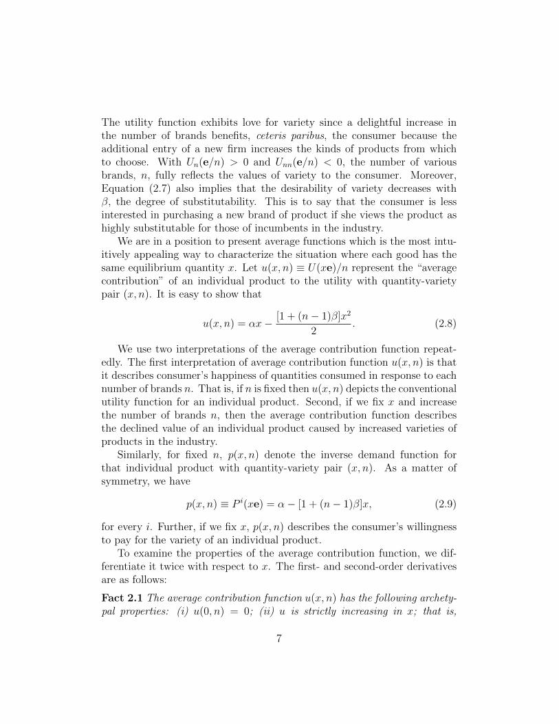
The utility function exhibits love for variety since a delightful increase inthe number of brands benefits, ceteris paribus, the consumer because theadditional entry of a new firm increases the kinds of products from whichto choose. With Un(e/n) > 0 and Unn(e/n) < 0, the number of variousbrands, n, fully reflects the values of variety to the consumer. Moreover,Equation (2.7) also implies that the desirability of variety decreases withβ, the degree of substitutability. This is to say that the consumer is lessinterested in purchasing a new brand of product if she views the product ashighly substitutable for those of incumbents in the industry.

We are in a position to present average functions which is the most intu-itively appealing way to characterize the situation where each good has thesame equilibrium quantity x. Let u(x, n) ≡ U(xe)/n represent the “averagecontribution” of an individual product to the utility with quantity-varietypair (x, n). It is easy to show that

u(x, n) = αx− [1 + (n− 1)β]x2

2. (2.8)

We use two interpretations of the average contribution function repeat-edly. The first interpretation of average contribution function u(x, n) is thatit describes consumer’s happiness of quantities consumed in response to eachnumber of brands n. That is, if n is fixed then u(x, n) depicts the conventionalutility function for an individual product. Second, if we fix x and increasethe number of brands n, then the average contribution function describesthe declined value of an individual product caused by increased varieties ofproducts in the industry.

Similarly, for fixed n, p(x, n) denote the inverse demand function forthat individual product with quantity-variety pair (x, n). As a matter ofsymmetry, we have

p(x, n) ≡ P i(xe) = α− [1 + (n− 1)β]x, (2.9)

for every i. Further, if we fix x, p(x, n) describes the consumer’s willingnessto pay for the variety of an individual product.

To examine the properties of the average contribution function, we dif-ferentiate it twice with respect to x. The first- and second-order derivativesare as follows:

Fact 2.1 The average contribution function u(x, n) has the following archety-pal properties: (i) u(0, n) = 0; (ii) u is strictly increasing in x; that is,

7

∂u(x, n)/∂x = p(x, n) > 0, and hence u(x, n) =∫ x0p(t, n)dt; (iii) u is strictly

concave in x in the sense that ∂2u(x, n)/∂x2 = −[1+(n−1)β] < 0, which im-plies ∂p(x, n)/∂x < 0; (iv) s(x, n) ≡ u(x, n)−xp(x, n) = [1+(n−1)β]x2/2 >0.

The condition u(0, n) = 0 means that the consumer has no utility whenconsuming nothing. In Part (ii) and (iii), we know that p behaves like an ordi-nary inverse demand function with u being its corresponding utility function.From (iii) of Fact 2.1, each firm faces a downward-slopping demand curvewith ∂p(x, n)/∂x < 0. In a word, it has market power to raise its price prof-itably. Part (iv) says that the total value of consumption of any individualproduct s(x, n), which is referred to as “average consumer surplus”, will yielda net benefit to the consumer for purchasing the good.

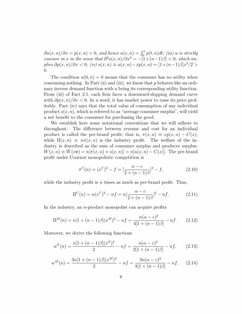
We establish here some notational conventions that we will adhere tothroughout. The difference between revenue and cost for an individualproduct is called the per-brand profit; that is, π(x, n) ≡ xp(x, n) − C(x),while Π(x, n) ≡ nπ(x, n) is the industry profit. The welfare of the in-dustry is described as the sum of consumer surplus and producer surplus:W (x, n) ≡ W (xe) = n[π(x, n) + s(x, n)] = n[u(x, n)−C(x)]. The per-brandprofit under Cournot monopolistic competition is

πC(n) = (xC)2 − f = [α− c

2 + (n− 1)β]2 − f, (2.10)

while the industry profit is n times as much as per-brand profit. Thus,

ΠC(n) = n(xC)2 − nf = n[α− c

2 + (n− 1)β]2 − nf. (2.11)

In the industry, an n-product monopolist can acquire profits

ΠM(n) = n[1 + (n− 1)β](xM)2 − nf =n(α− c)2

4[1 + (n− 1)β]− nf. (2.12)

Moreover, we derive the following functions

wF (n) =n[1 + (n− 1)β](xF )2

2− nf =

n(α− c)2

2[1 + (n− 1)β]− nf, (2.13)

wM(n) =3n[1 + (n− 1)β](xM)2

2− nf =

3n(α− c)2

8[1 + (n− 1)β]− nf, (2.14)

8

and

wC(n) =n[3 + (n− 1)β](xC)2

2−nf =

n[3 + (n− 1)β](α− c)2

2[2 + (n− 1)β]2−nf (2.15)

for welfare analysis.The discussion then turns to determine the optimal number of brands

for different types of market that exist. The equilibrium number of brandsis determined within the model by entry behavior: The socially first-bestnumber of brands is nF ≡ arg maxnw

F (n), whereas the optimal number ofbrands for the monopolist is nM ≡ arg maxn ΠM(n). In a Cournot marketwithout barriers to entry, we ignore the integer problem and assume thatfirms enter the industry until economic profits are driven exactly to zero.Then the equilibrium number of brands existing in the industry, nC , is givenby πC(nC) = 0.

3 Equilibrium Quantity-Variety Pairs

Before the start of discussion, let us ascertain whether the solutions are welldefined and see what regularity conditions of fixed costs for keeping varietiesin the industry are to be.

Fact 3.1 (i) Both functions wF (n) and ΠM(n) are strictly concave, i.e.,wFnn(n) < 0 and ΠM

nn(n) < 0, for all n; (ii) πCn (n) < 0, for all n. (See theproof in Appendix.)

As Part (i) shown, both nF and nM are well defined in the sense that theycan be obtained by solving th first-order conditions wFn (n) = 0 if wFn (0) ≥ 0,and ΠM

n (n) = 0 if ΠMn (0) ≥ 0. Part (ii) of Fact 3.1 tells us the profit for

any particular product is squeezed down when a new brand is introducedto the market. The condition guarantees the unique existence of Cournotequilibrium and if, a dynamic process n = µCπC(n) is assumed, where µC

is a positive constant, it also implies that the dynamic process is globallystable.

Judging straightforwardly from Fact 3.1, we know that the industry pro-vides a variety of products, not a tedious sameness, whenever wFn (1) > 0 forfirst-best optimum, ΠM

n (1) > 0 for monopoly, and πC(1) > 0 for Cournotmonopolistic competition, respectively. Then we derive sufficient conditionsin the following proposition to help build intuition and to present more in-teresting results.

9

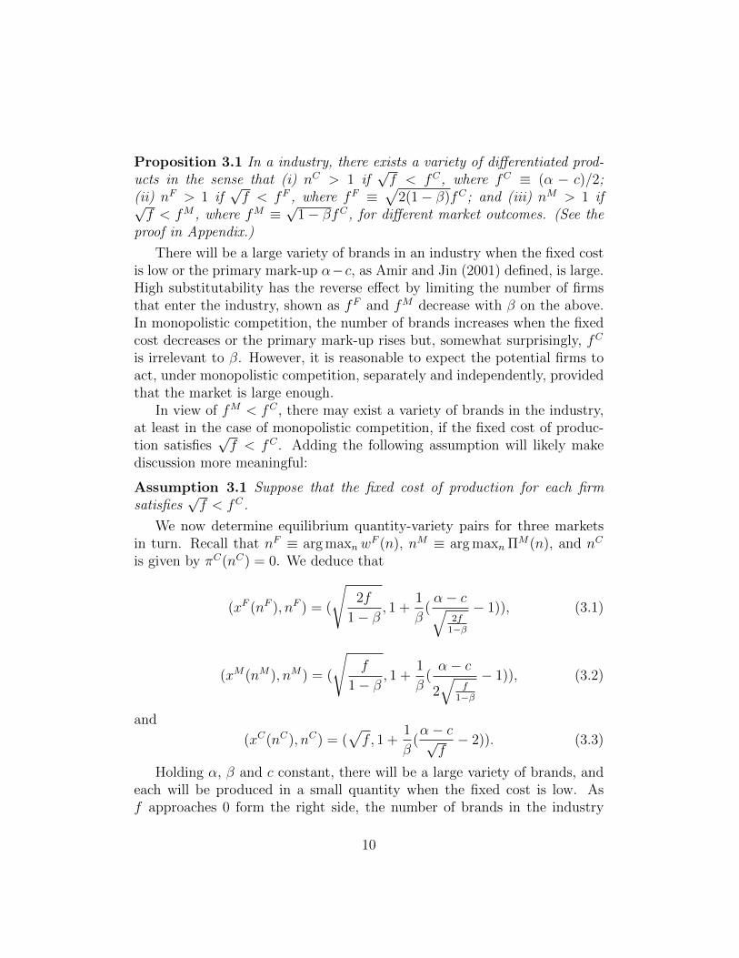
Proposition 3.1 In a industry, there exists a variety of differentiated prod-ucts in the sense that (i) nC > 1 if

√f < fC, where fC ≡ (α − c)/2;

(ii) nF > 1 if√f < fF , where fF ≡

√2(1− β)fC; and (iii) nM > 1 if√

f < fM , where fM ≡√

1− βfC, for different market outcomes. (See theproof in Appendix.)

There will be a large variety of brands in an industry when the fixed costis low or the primary mark-up α−c, as Amir and Jin (2001) defined, is large.High substitutability has the reverse effect by limiting the number of firmsthat enter the industry, shown as fF and fM decrease with β on the above.In monopolistic competition, the number of brands increases when the fixedcost decreases or the primary mark-up rises but, somewhat surprisingly, fC

is irrelevant to β. However, it is reasonable to expect the potential firms toact, under monopolistic competition, separately and independently, providedthat the market is large enough.

In view of fM < fC , there may exist a variety of brands in the industry,at least in the case of monopolistic competition, if the fixed cost of produc-tion satisfies

√f < fC . Adding the following assumption will likely make

discussion more meaningful:

Assumption 3.1 Suppose that the fixed cost of production for each firmsatisfies

√f < fC.

We now determine equilibrium quantity-variety pairs for three marketsin turn. Recall that nF ≡ arg maxnw

F (n), nM ≡ arg maxn ΠM(n), and nC

is given by πC(nC) = 0. We deduce that

(xF (nF ), nF ) = (

√2f

1− β, 1 +

1

β(α− c√

2f1−β

− 1)), (3.1)

(xM(nM), nM) = (

√f

1− β, 1 +

1

β(α− c

2√

f1−β

− 1)), (3.2)

and

(xC(nC), nC) = (√f, 1 +

1

β(α− c√f− 2)). (3.3)

Holding α, β and c constant, there will be a large variety of brands, andeach will be produced in a small quantity when the fixed cost is low. Asf approaches 0 form the right side, the number of brands in the industry

10

approaches infinity and the equilibrium output approaches zero in all cases.But, Equations (3.1) and (3.2) together imply that

(nF − 1)β + 1

(nM − 1)β + 1=√

2 =xF (nF )

xM(nM). (3.4)

Therefore, (xF (nF ), nF ) and (xM(nM), xM) share the same structure in thesense nF/nM u xF (nF )/xM(nM) when f is small enough. This is not onlyinteresting in its own right, it is essential for proving deeper structural prop-erties. The discussion will be provided in later sections.

4 Comparison Among Three Equilibria

We proceed in this section to compare the three equilibria derived above tojudge their competitiveness.

Proposition 4.1 For three pairs of equilibrium quantity-variety, (xF (nF ), nF ),(xM(nM), nM) and (xC(nC), nC), we have (i) All equilibrium prices pF , pM ,and pC do not depend on the number of varieties n: pF = c, pM = c + (α −c)/2 = (α+c)/2, and pC = c+

√f . Moreover, pF < pC < pM . (ii) The rank-

ing of the three for equilibrium quantities is xC(nC) < xM(nM) < xF (nF ).(iii) From the viewpoint of the total output in the industry, the total quantityof Cournot equilibrium lies between those of the monopoly solution and thefirst-best solution in the sense that nMxM(nM) < nCxC(nC) < nFxF (nF ).(See the proof in Appendix.)

Clearly, we know that, given all number of brands n, xC(n) > xM(n) andthat both xM(n) and xC(n) decrease with n. Part (ii) of Proposition 4.1states that a reversal of the Cournotmonopoly equilibrium quantity orderingcan occur under assumption of endogenous entry; that is, xC(nC) < xM(nM).This reversal arises because with free entry, a large firms may find it profitableto enter the industry and leave less room for an individual firm to serve themarket. It is easily verified that nC > nM from (ii) and (iii) of Proposition4.1. Moreover, Equation (4.4) indicates that nM < nF and so it remains tocompare nC with nF .

Let us define fCF = (α − c)[2 −√

2(1− β)]/2 ≡ [2 −√

2(1− β)]fC . Itis easily to show that

nC T nF ⇔√f S fCF

11

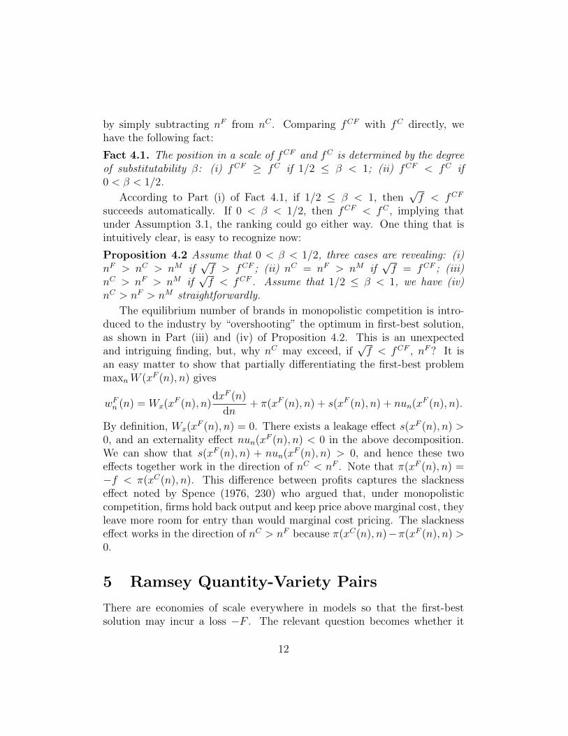
by simply subtracting nF from nC . Comparing fCF with fC directly, wehave the following fact:

Fact 4.1. The position in a scale of fCF and fC is determined by the degreeof substitutability β: (i) fCF ≥ fC if 1/2 ≤ β < 1; (ii) fCF < fC if0 < β < 1/2.

According to Part (i) of Fact 4.1, if 1/2 ≤ β < 1, then√f < fCF

succeeds automatically. If 0 < β < 1/2, then fCF < fC , implying thatunder Assumption 3.1, the ranking could go either way. One thing that isintuitively clear, is easy to recognize now:

Proposition 4.2 Assume that 0 < β < 1/2, three cases are revealing: (i)nF > nC > nM if

√f > fCF ; (ii) nC = nF > nM if

√f = fCF ; (iii)

nC > nF > nM if√f < fCF . Assume that 1/2 ≤ β < 1, we have (iv)

nC > nF > nM straightforwardly.

The equilibrium number of brands in monopolistic competition is intro-duced to the industry by “overshooting” the optimum in first-best solution,as shown in Part (iii) and (iv) of Proposition 4.2. This is an unexpectedand intriguing finding, but, why nC may exceed, if

√f < fCF , nF ? It is

an easy matter to show that partially differentiating the first-best problemmaxnW (xF (n), n) gives

wFn (n) = Wx(xF (n), n)

dxF (n)

dn+ π(xF (n), n) + s(xF (n), n) + nun(xF (n), n).

By definition, Wx(xF (n), n) = 0. There exists a leakage effect s(xF (n), n) >

0, and an externality effect nun(xF (n), n) < 0 in the above decomposition.We can show that s(xF (n), n) + nun(xF (n), n) > 0, and hence these twoeffects together work in the direction of nC < nF . Note that π(xF (n), n) =−f < π(xC(n), n). This difference between profits captures the slacknesseffect noted by Spence (1976, 230) who argued that, under monopolisticcompetition, firms hold back output and keep price above marginal cost, theyleave more room for entry than would marginal cost pricing. The slacknesseffect works in the direction of nC > nF because π(xC(n), n)−π(xF (n), n) >0.

5 Ramsey Quantity-Variety Pairs

There are economies of scale everywhere in models so that the first-bestsolution may incur a loss −F . The relevant question becomes whether it

12

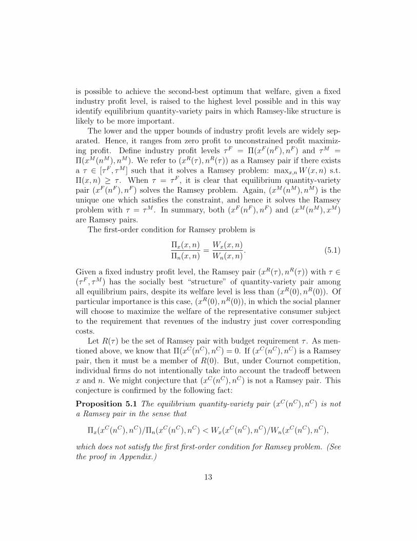
is possible to achieve the second-best optimum that welfare, given a fixedindustry profit level, is raised to the highest level possible and in this wayidentify equilibrium quantity-variety pairs in which Ramsey-like structure islikely to be more important.

The lower and the upper bounds of industry profit levels are widely sep-arated. Hence, it ranges from zero profit to unconstrained profit maximiz-ing profit. Define industry profit levels τF = Π(xF (nF ), nF ) and τM =Π(xM(nM), nM). We refer to (xR(τ), nR(τ)) as a Ramsey pair if there existsa τ ∈ [τF , τM ] such that it solves a Ramsey problem: maxx,nW (x, n) s.t.Π(x, n) ≥ τ . When τ = τF , it is clear that equilibrium quantity-varietypair (xF (nF ), nF ) solves the Ramsey problem. Again, (xM(nM), nM) is theunique one which satisfies the constraint, and hence it solves the Ramseyproblem with τ = τM . In summary, both (xF (nF ), nF ) and (xM(nM), xM)are Ramsey pairs.

The first-order condition for Ramsey problem is

Πx(x, n)

Πn(x, n)=Wx(x, n)

Wn(x, n). (5.1)

Given a fixed industry profit level, the Ramsey pair (xR(τ), nR(τ)) with τ ∈(τF , τM) has the socially best “structure” of quantity-variety pair amongall equilibrium pairs, despite its welfare level is less than (xR(0), nR(0)). Ofparticular importance is this case, (xR(0), nR(0)), in which the social plannerwill choose to maximize the welfare of the representative consumer subjectto the requirement that revenues of the industry just cover correspondingcosts.

Let R(τ) be the set of Ramsey pair with budget requirement τ . As men-tioned above, we know that Π(xC(nC), nC) = 0. If (xC(nC), nC) is a Ramseypair, then it must be a member of R(0). But, under Cournot competition,individual firms do not intentionally take into account the tradeoff betweenx and n. We might conjecture that (xC(nC), nC) is not a Ramsey pair. Thisconjecture is confirmed by the following fact:

Proposition 5.1 The equilibrium quantity-variety pair (xC(nC), nC) is nota Ramsey pair in the sense that

Πx(xC(nC), nC)/Πn(xC(nC), nC) < Wx(x

C(nC), nC)/Wn(xC(nC), nC),

which does not satisfy the first first-order condition for Ramsey problem. (Seethe proof in Appendix.)

13

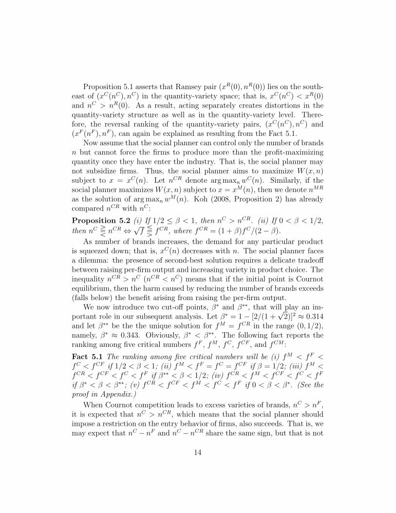
Proposition 5.1 asserts that Ramsey pair (xR(0), nR(0)) lies on the south-east of (xC(nC), nC) in the quantity-variety space; that is, xC(nC) < xR(0)and nC > nR(0). As a result, acting separately creates distortions in thequantity-variety structure as well as in the quantity-variety level. There-fore, the reversal ranking of the quantity-variety pairs, (xC(nC), nC) and(xF (nF ), nF ), can again be explained as resulting from the Fact 5.1.

Now assume that the social planner can control only the number of brandsn but cannot force the firms to produce more than the profit-maximizingquantity once they have enter the industry. That is, the social planner maynot subsidize firms. Thus, the social planner aims to maximize W (x, n)subject to x = xC(n). Let nCR denote arg maxnw

C(n). Similarly, if thesocial planner maximizes W (x, n) subject to x = xM(n), then we denote nMR

as the solution of arg maxnwM(n). Koh (2008, Proposition 2) has already

compared nCR with nC :

Proposition 5.2 (i) If 1/2 ≤ β < 1, then nC > nCR. (ii) If 0 < β < 1/2,

then nC T nCR ⇔√f S fCR, where fCR = (1 + β)fC/(2− β).

As number of brands increases, the demand for any particular productis squeezed down; that is, xC(n) decreases with n. The social planner facesa dilemma: the presence of second-best solution requires a delicate tradeoffbetween raising per-firm output and increasing variety in product choice. Theinequality nCR > nC (nCR < nC) means that if the initial point is Cournotequilibrium, then the harm caused by reducing the number of brands exceeds(falls below) the benefit arising from raising the per-firm output.

We now introduce two cut-off points, β∗ and β∗∗, that will play an im-portant role in our subsequent analysis. Let β∗ = 1− [2/(1 +

√2)]2 ≈ 0.314

and let β∗∗ be the the unique solution for fM = fCR in the range (0, 1/2),namely, β∗ ≈ 0.343. Obviously, β∗ < β∗∗. The following fact reports theranking among five critical numbers fF , fM , fC , fCF , and fCM :

Fact 5.1 The ranking among five critical numbers will be (i) fM < fF <fC < fCF if 1/2 < β < 1; (ii) fM < fF = fC = fCF if β = 1/2; (iii) fM <fCR < fCF < fC < fF if β∗∗ < β < 1/2; (iv) fCR < fM < fCF < fC < fF

if β∗ < β < β∗∗; (v) fCR < fCF < fM < fC < fF if 0 < β < β∗. (See theproof in Appendix.)

When Cournot competition leads to excess varieties of brands, nC > nF ,it is expected that nC > nCR, which means that the social planner shouldimpose a restriction on the entry behavior of firms, also succeeds. That is, wemay expect that nC − nF and nC − nCR share the same sign, but that is not

14

strictly true: Comparing Fact 5.1 with Proposition 4.2 shows that the rankingof nC and nCR is indeed the case when 1/2 ≤ β < 1. But, if 0 < β < 1/2,then, according to Part (ii)-(iv) of Fact 5.1, it is possible that fCR < fCF <fC under Assumption 3.1, which implies that (nC −nF )(nC −nCR) < 0. Wesummarize our results in the following proposition:

Proposition 5.3 (i) If 0 < β < 1/2 and fCR <√f < fCF , then nC−nF and

nC − nCR have the opposite signs, namely, nC − nF > 0 and nC − nCR < 0.(ii) Otherwise, (nC − nF )(nC − nCR) ≥ 0.

In Case (i), somewhat surprisingly, the social planner should somehowraise the number of brands although Cournot competition already leads toexcess varieties. We now formally discuss the question whether the over-shooting result is socially desirable.

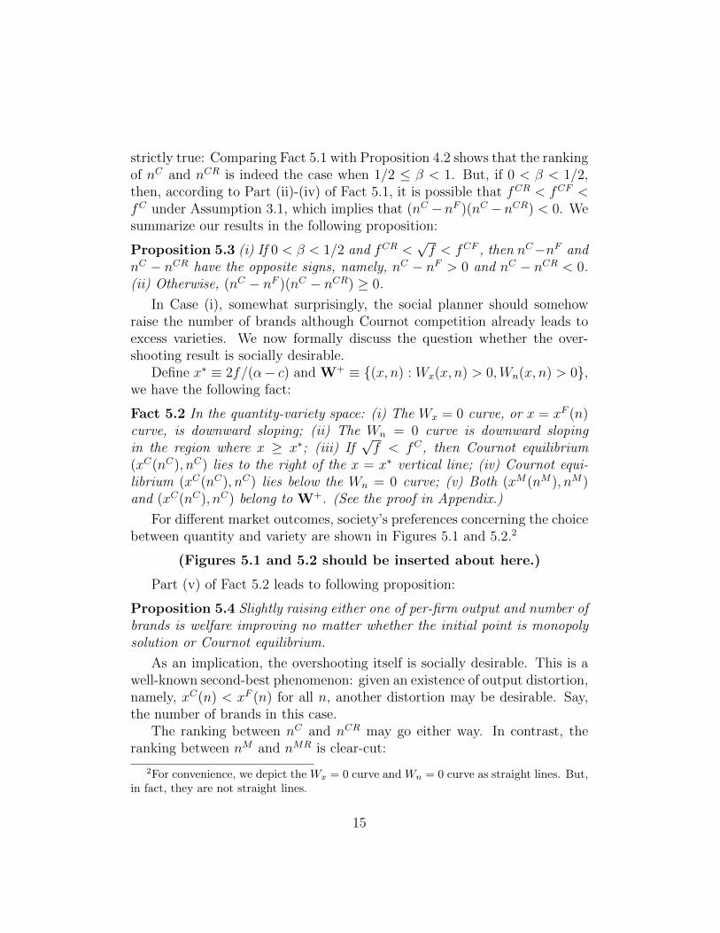
Define x∗ ≡ 2f/(α− c) and W+ ≡ {(x, n) : Wx(x, n) > 0,Wn(x, n) > 0},we have the following fact:

Fact 5.2 In the quantity-variety space: (i) The Wx = 0 curve, or x = xF (n)curve, is downward sloping; (ii) The Wn = 0 curve is downward slopingin the region where x ≥ x∗; (iii) If

√f < fC, then Cournot equilibrium

(xC(nC), nC) lies to the right of the x = x∗ vertical line; (iv) Cournot equi-librium (xC(nC), nC) lies below the Wn = 0 curve; (v) Both (xM(nM), nM)and (xC(nC), nC) belong to W+. (See the proof in Appendix.)

For different market outcomes, society’s preferences concerning the choicebetween quantity and variety are shown in Figures 5.1 and 5.2.2

(Figures 5.1 and 5.2 should be inserted about here.)

Part (v) of Fact 5.2 leads to following proposition:

Proposition 5.4 Slightly raising either one of per-firm output and number ofbrands is welfare improving no matter whether the initial point is monopolysolution or Cournot equilibrium.

As an implication, the overshooting itself is socially desirable. This is awell-known second-best phenomenon: given an existence of output distortion,namely, xC(n) < xF (n) for all n, another distortion may be desirable. Say,the number of brands in this case.

The ranking between nC and nCR may go either way. In contrast, theranking between nM and nMR is clear-cut:

2For convenience, we depict the Wx = 0 curve and Wn = 0 curve as straight lines. But,in fact, they are not straight lines.

15

Proposition 5.5 (i) nM < nMR; (ii) nF −nM and nMR−nM share the samesign. (See the proof in Appendix.)

This proposition unambiguously states that the social planner shouldrequest that the monopoly raises varieties if the social planner can controlfor the number of brands. Further, Propositions 4.2, 5.2 and 5.5 togetherimply the following proposition:

Proposition 5.6 (i) Assume that If β∗∗ < β < 1. If√f < fM , then each

solution is interior with nC > nF > nM , nC > nCR, and nMR > nM . (ii)Assume that β∗ < β < β∗∗. If

√f < fM , then each solution is interior

with nC > nF > nM , and nMR > nM . Moreover, there are two subcasescorresponding to the second case: (a) if

√f < fCR, then nC > nCR; (b) if√

f > fCR, then nC < nCR. (iii) Assume that 0 < β < β∗. If√f < fM ,

then each solution is interior with nF > nM , and nMR > nM . There arethree possible subcases: (a) if

√f < fCR, then nC > nF and nC > nCR; (b)

if fCR <√f < fCF , then nC > nF and nC < nCR; (c) if

√f > fCF , then

nC < nF and nC < nCR.

We are in a position to discuss the structure of quantity-variety pair(x, n). The monopoly always moves these two numbers in the same direction:nM < nF and xM(nM) < xF (nF ). In contrast, Cournot competition maymove these two numbers in opposite directions: for example, in Case (i), nC >nF and xC(nC) < xF (nF ) (more strikingly, xC(nC) < xM(nM)). It shouldbe concluded, from what has been said above, that Cournot competitiondistorts the structure of (x, n). If Cournot equilibrium happens to be aRamsey outcome, then it is welfare superior than the monopoly solution.Unfortunately, Cournot equilibrium is not a Ramsey outcome. Therefore, itis noteworthy that the monopoly solution may be better off than Cournotequilibrium.

6 Conclusion

This paper compares the competitiveness and welfare implications of mo-nopolistic competition with first-best solution and monopoly outcome. Therelevant factors considered in this paper includes the substitutability amongproducts, the size of fixed costs, conditions for free entry. We find that, undermonopolistic competition, potential firms will enter the industry than whatwould be socially optimal. In this case, the social planner, if exists, may fur-

16

ther raise varieties since, given lower equilibrium output level than first-bestoutcome, a larger variety of brands may be welfare improving. That is tosay, the overshooting in varieties is socially desirable. Second, our resultsagree with the well-known claim that Cournot equilibrium is more competi-tive than monopoly equilibrium in the sense that the Cournot outcome haslower prices, greater number of varieties, and greater industry total outputsthan those of monopoly solution. But, Cournot equilibrium is more intrinsi-cally better off than monopoly solution may not be true since the Cournotoutcome has a distorted quantity-variety structure. Having suggested thatthe welfare ranking between these two solutions is not obvious, we still havea long way to go before we arrive at an interpretation of conditions thatmonopoly outcome is indeed welfare efficient than Cournot equilibrium.

17

ReferencesChang, M. C., “An Asymmetric Oligopolist can Improve Welfare by Raising

Price,” Review of Industrial Organization, 2010, 36(1), 75-96.

Chang, M. C. and Peng, H.-P., “Structure Regulation, Price Structure,Cross Subsidization and Marginal Cost of Public Funds,” The Manch-ester School, 77(6), 675698.

Chang, M. C. and Peng, H.-P., “Cournot and Bertrand Equilibria Com-pared: A Critical Review and an Extension from the Output-structureViewpoint,” Japanese Economic Review, Forthcoming, 2011.

Dixit, A. K. and Stiglitz, J. E., “Monopolistic Competition and OptimumProduct Diversity,” American Economic Review, 1977, 67(3), 297-308.

Koh, W. T. H., “Market Competition, Social Welfare in an Entry-ConstrainedDifferentiated-Good Oligopoly,” Economics Letters, 2008, 100(2), 229-233.

Spence, A. M., “Product Selection, Fixed Costs, and Monopolistic Compe-tition,” Review of Economic Studies, 1976, 43(2), 217-236.

Stiglitz, J. E., “Potential Competition May Reduce Welfare,” American Eco-nomic Review: Papers and Proceedings, 1981, 71(2), 184-189.

Tirole, J. The theory of industrial organization, 1988. Cambridge, MA: MITPress.

Vickers, J., “Competition and Regulation in Vertically Related Markets,”Review of Economic Studies, 1995, 62, 1-17.

18

AppendixProof of Fact 3.1. We differentiate Equation (2.13) twice with respect ton and we get

wFnn(n) = − β(1− β)2

[1 + (n− 1)β]3< 0,

and the second-order derivative of Equation (2.12) gives

ΠMnn(n) = −β(1− β)(α− c)2

2[1 + (n− 1)β]3< 0.

Therefore, we know that wF (n) and ΠM(n) are strictly concave. Once Again,by differentiating Equation (2.10) with respect to n,

πCn (n) = − 2β(α− c)2

[2 + (n− 1)β]3< 0

follows. Q.E.D.

Proof of Proposition 3.1.(i): Substituting n = 1 into Equation (2.10), we obtain

πC(1) = (α− c

2)2 − f.

If the industry with single provider leaves room for potential competitorsto make profits, then free-entry equilibrium allows a reasonable number ofbrands supplier to enter the market. That is, if πC(1) > 0 or

√f < fC , then

nC > 1.(ii): Differentiating Equation (2.13) yields

wFn (n) =1− β

2(

α− c1 + (n− 1)β

)2 − f.

With wFnn(n) < 0, as mentioned in Part (i) of Fact 3.1, if wFn (1) > 0 or√f < fF , then there exists nF > 1 such that wFn (nF ) = 0.

(iii): Analogously, differentiating Equation (2.12) yields

ΠMn (n) =

1− β4

(α− c

1 + (n− 1)β)2 − f.

With ΠMnn(n) < 0, as mentioned in Part (i) of Fact 3.1, if ΠM

n (1) > 0 or√f < fM , then there exists nM > 1 such that ΠM

n (nM) = 0. Q.E.D.

19

Proof of Proposition 4.1.(i) Substituting Equation (3.1), (3.2), and (3.3) into (2.9) give pF = c,

pM = c + (α − c)/2 = (α + c)/2, and pC = c +√f , respectively. Obviously,

pF < pC < pM because√f < (α− c)/2.

(ii) According to (3.1), (3.2), and (3.3), it is clear that xC(nC) < xM(nM) <xF (nF ) since 1− β < 1.

(iii) According to (3.1), (3.2), and (3.3), we have

nFxF (nF ) = (1− 1

β)

√2f

1− β+

(α− c)β

, (A.1)

nMxM(nM) = (1− 1

β)

√f

1− β+

(α− c)2β

, (A.2)

and

nCxC(nC) = (1− 2

β)√f +

(α− c)β

, (A.3)

Subtracting (A.3) from (A.1) leads to

nFxF (nF )− nCxC(nC) =√f [

2

β− 1−

√2(1− β)

β].

We can utilize MATLAB to show that 2/β − 1 −√

2(1− β)/β > 0, for all0 < β < 1. Next, subtracting (A.2) from (A.3) gives

nCxC(nC)− nMxM(nM) =1

β{α− c

2+√f [β − 2 +

√1− β]},

We can utilize MATLAB to show that −1 < β− 2 +√

1− β ≤ −0.75, for all0 < β < 1. Therefore, it follows that {·} > 0 since

√f < (α− c)/2. Q.E.D.

Proof of proposition 5.1. In monopolist competition, the industry profitand total welfare are

ΠC(x, n) = n{(α− c)x− [1 + (n− 1)β]x2 − f},

and

wC(x, n) = n{(α− c)x− [1 + (n− 1)β]x2

2− f}.

20

Partially differentiating ΠC(x, n) with respect to x and n, respectively, at(xC(nC), nC) gives ΠC

x (xC(nC), nC) = n[2√f − (α − c)] = [1 + (α − c)/β −

2/β][2√f − (α − c)] < 0, and ΠC

n (xC(nC), nC) = −nβf = −βf [1 + (α −c)/β − 2/β] < 0 since

√f < fC ≡ (α− c)/2. Combining the above, we get

ΠCx (xC(nC), nC)

ΠCn (xC(nC), nC)

=(α− c)− 2

√f

βf> 0.

Analogously, partially differentiating wC(x, n) with respect to x and n,respectively, at (xC(nC), nC), we have wCx (xC(nC), nC) = n

√f = f [1 + (α−

c)/β−2/β] > 0, and ΠCn (xC(nC), nC) = (1−β)f/2 > 0. Dividing the former

by the latter yields

wCx (xC(nC), nC)

wCn (xC(nC), nC)=

2β√f + 2(α− c)− 4

√f

β(1− β)f> 0.

The proof of this fact is complete by directly deducting the two items:

wCx (xC(nC), nC)

wCn (xC(nC), nC)− ΠC

x (xC(nC), nC)

ΠCn (xC(nC), nC)

=1

β(1− β)f[(1 + β)(α− c)− 2

√f ]

>1

β(1− β)f[(1 + β)(α− c)− (α− c)]

=(α− c)

(1− β)f

> 0

because√f < (α− c)/2. Q.E.D.

Proof of Fact 5.1 (i): From 1 − β > 0, it follows that fF > fM andfC > fM . In order to prove Part (i), it remains to show that fF < fC < fCF .Note that β > 1/2 implies

√2(1− β) < 1. Thus, 2 −

√2(1− β) > 1. It

follows that fF < fC < fCF .(ii): β = 1/2 implies

√2(1− β) = 2−

√2(1− β) = 1.

(iii)-(v): Note that β < 1/2 implies√

2(1− β) > 1. Thus, 2−√

2(1− β) <

1. Therefore, fF > fC > fCF . Moreover, fCF > fM if 2 −√

2(1− β) >√1− β. It is equivalent to β∗ < β. fCR > fM if (1 + β)/(2 − β) >√1− β or (1 + β)2/(2 − β)2 > 1 − β. It is equivalent to f(β) > 0, where

21

f(β) = β3 − 4β2 + 10β − 3. We know that f(0) = −3, f(1/2) = 9/8, andf ′(β) = 3β2 − 8β + 10 > 0 for all 0 < β ≤ 1/2. Therefore, there exists aunique solution for f(β) = 0 in the range (0, 1/2). It is easy to show thatfCF − fCR = 0, for β = 1/2, and fCF − fCR strictly decreases with β, andhence fCF − fCR > 0, for all 0 < β < 1/2. Q.E.D.

Proof of Fact 5.2. Part (i) is clear.(ii): The slope of the Wn curve is equal with −Wnx/Wnn. Because Wnn <

0, it suffices to show that Wnx is strictly negative when Wn = 0. FromWn = 0, it follows that [1 + (2n − 1)β]x = 2(α − c) − 2f/x. Therefore,Wxn = −(α− c) + 2f/x, which is strictly negative if x > x∗.

(iii): It is easy to show√f > 2f/(α − c) if and only if (α − c)/2 >

√f .

This means that√f = xC(nC) > x∗ if and only if

√f < fC .

(iv): We establish that Wn(xC(nC), nC) > 0. Because xC(nC) =√f , we

can replace f in Wn by x2 to obtain Wn = (α−c)x−[1+(2n−1)β]x2/2−x2 =(α− c)x− [3 + (2n− 1)β]x2/2. It is clear that Wn shares the same sign with(α−c)− [3+(2n−1)β]x/2, which is equal to (α−c)(1−β)/{2[2+(n−1)β]}if we replace x by xC(n).

(v): xM(n) < xC(n) < xF (n) for all n. It follows that both (xM(nM), nM)and (xC(nC), nC) lie in the left of theWx = 0 curve. Because (xM(nM), nM) <(xF (nF ), nF ) and Wn = 0 curve is downward sloping, (xM(nM), nM) lies be-low the Wn = 0 curve. Moreover, Part (iv) states that (xC(nC), nC) liesbelow the Wn = 0 curve. Therefore, Part (v) follows from Wxx < 0 andWnn < 0. Q.E.D.

Proof of Proposition 5.5. As mentioned above, Wx = n(p − c). We canshow that, in the monopoly solution, p − c is simply equal to (α − c)/2.We also can show that dxM(n)/dn = −(α − c)β/{2[1 + (n − 1)β]2}, andhence Wxdx

M(n)/dn = −n(α−c)2β/{4[1+(n−1)β]2}. Moreover, s+nsn =[1+(2n−1)β](α−c)2/{8[1+(n−1)β]2}. Therefore, Wxdx

M(n)/dn+s+nsnis equal with (1− β)(α− c)2/{8[1 + (n− 1)β]2}. Q.E.D.

22

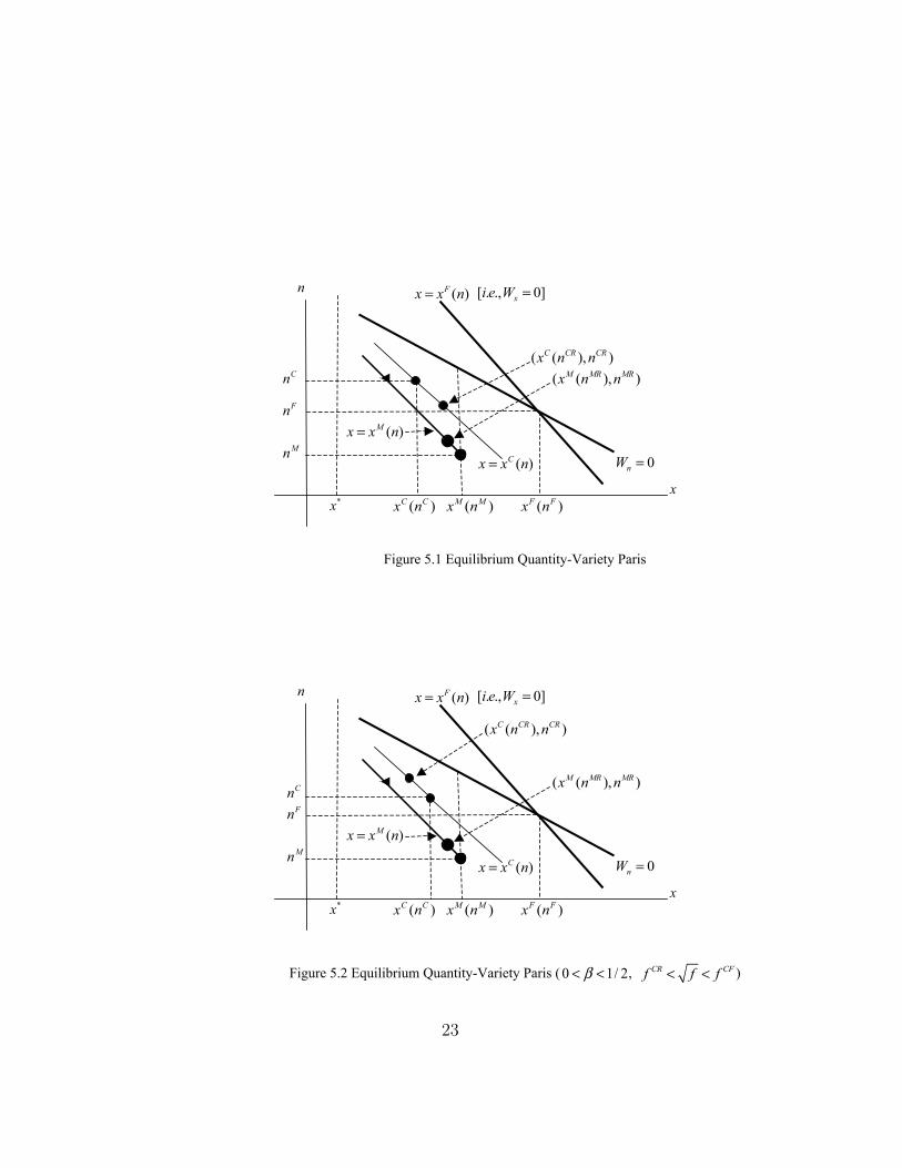
Figure 5.1 Equilibrium Quantity-Variety Paris

Figure 5.2 Equilibrium Quantity-Variety Paris (0 1/ 2β< < , CR CFf f f< < )

*x )( FF nx

Fn

n

x

)(nxx F=

0=nW

]0.,.[ =xWei

)(nxx M=

)(nxx C=

)( MM nx

Mn

)( CC nx

Cn

( ( ), )C CR CRx n n

( ( ), )M MR MRx n n

*x )( FF nx

Fn

n

x

)(nxx F=

0=nW

]0.,.[ =xWei

)(nxx M=

)(nxx C=

)( MM nx

Mn

)( CC nx

Cn( ( ), )C CR CRx n n( ( ), )M MR MRx n n

23