Comparison and Validation of Several Open Access Remotely ...

Comparison and Validation of Several Open Access Remotely Sensed Rainfall Products for the Nile Basin

Tim Martijn Hessels

Delft

Univ

ers

ity o

f Tech

nolo

gy

Mast

er

of

Sci

ence

Thesi

s

Photo cover: http://miriadna.com/desctopwalls/images/max/Astronomy-sky.jpg

Comparison and Validation of Several Open Access Remotely Sensed

Rainfall Products for the Nile Basin

By

T.M. Hessels

Studentnumber: 4030389

in partial fulfillment of the requirements for the degree of

Master of Science in Civil Engineering

at the Delft University of Technology,

to be defended publicly on Monday February 2, 2015 at 15:00 AM.

Thesis committee: prof. dr. W.G.M. Bastiaanssen, TU Delft & IHE-UNESCO Dr. ir. R. Hut, TU Delft

Prof. dr. Y. Mohamed, IHE-UNESCO Prof. dr. ir. H Russchenberg, TU Delft

An electronic version of this thesis is available at http://repository.tudelft.nl/.

Preface This report/paper is the result of my master thesis project, which is part of the master Water

Management at the University of Technology Delft. During the last 10 months, I have investigated

the differences of the open access remotely sensed rainfall product for the Nile Basin. In this period I

learned a lot, which could not be achieved without the help and support of many people.

First of all, I would like to thank all the members of my graduation committee for the guidance and

useful advices that they gave me during the whole project. I want to thank Wim Bastiaanssen

especially for the daily support and the help with searching contacts to receive the ground data.

Without this data this research could not be done. I would like to thank Yasir Mohamed, Zheng Duan,

and Peter Droogers for sending me the required ground rainfall data. I also want to thank Rolf Hut for

editing/reviewing my main article and for all the useful advice you gave me to improve this study.

Last but not least, I would like to thank my family, friends and all other people that have supported

and promoted me during my thesis work. I am very proud of the end results and I hope the reader

enjoys reading it.

Tim Hessels Delft, January 2015

Summary More and more countries suffer from water stress and water scarcity problems. This is due to the

increasing water demand which is the result of the population and economic growth. Therefore,

countries have to improve their water efficiency. This requires a lot of research to give more insight

in the local water and energy cycles. A simple tool to provide the required information is the Water

Accounting plus framework. This framework requires a lot of hydrological and geographical data,

which are for some continents hard to obtain from ground measurements only. This is the case in

Africa for example. This makes satellite measurements a very attractive open access data source for

this framework. But with different products on the market the question is which of the open access

data sources gives the best estimate? In this research the open access rainfall estimation products

are validated and compared.

In total, 13 open access rainfall products are compared and validated with the use of 62 ground

measurements distributed over the Nile Basin. The validation period is from January 2000 to

December 2010. Also a 14th ensemble product is added which is made with the use of the estimated

relative errors calculated with the triple collocation method.

From the findings, one can conclude that the CHIRPS v1.8 product shows the best correlation and

root mean square error for the Nile Basin, while the bias suggests that this product underestimates

rainfall a bit. The more popular TRMM3B43 v7 product shows also good results, and has a very good

bias. The CHIRPS v1.8 product can be improved by removing the bias with the use of TRMM3B43 v7

data. Challenging would be to improve the spatial resolution of the product further by using other

satellite data for example a NDVI map. The ensemble product shows also good results for the

validations done on a coarser spatial grid, for the finer spatial grids the results were less promising.

This can be explained by the fact that the triple collocation was performed also on a coarser spatial

grid, this was needed to meet all the criteria of the triple collocation method.

This report consists of 4 parts. The first part consists of the main article of my research and has a scientific paper format, this document is called “Comparison and Validation of Several Open Access Remotely Sensed Rainfall Products for the Nile Basin”. The other 3 parts consist of supporting materials for this scientific paper. The second part is called “Basic Principles of Satellite Precipitation Measurements” and gives more information about the basics techniques of satellite rainfall measurements and will give some insight in the satellite algorithms. The third part gives some more information about the triple collocation method, this document is named “Triple collocation”. The last part called “Matlab m-files” consists of all the m-files which are used for the scientific paper to make, compare and validate the products. Those files can be opened in Matlab to perform the calculations done in the scientific paper.

Comparison and Validation of Several Open Access Rainfall Products for the Nile Basin Main Article

TU Delft Tim M. Hessels Supervisor: Prof. Dr. Wim G.M. Bastiaanssen

1

Comparison and Validation of Several Open Access Remotely Sensed Rainfall Products for the Nile Basin

T.M. Hesselsa

a Delft University of Technology, Department of Water Management, Stevinweg 1, Delft, The Netherlands

Abstract This paper describes a comparison and validation of 10 existing open-access and spatially distributed satellite rainfall products, 2 ground based products and 1 modeled rainfall product. The validation was performed for the Nile basin by using 62 ground-based rain gauge measurements across rainfall zones varying from 50 to 1800 mm/year. Special attention was paid to the Blue Nile sub basin, which is characterized by complex rainfall patterns. The rainfall products can be categorized into calibrated products where the biased is partially removed, and into biased products where no ground measurements have been consulted. The monthly validation across the entire Nile basin for a 0.25 degree spatial resolution reveals that the individual CMORPH product performs the best for the biased products (Monthly 0.25°: r=0.76; RMSE=80.1%.; bias=15.8mm). For the unbiased products, the CHIRPS v1.8 product is superior (Monthly 0.25°: r=0.92; RMSE=49.3%; bias=-14.6mm). The common TRMM 3B43 v7 product (Monthly 0.25°: r=0.89; RMSE=52.3%; bias=-3mm) has a better bias than CHIRPS v1.8. The best products over rugged terrain with complex rainfall patterns in the Blue Nile basin are also TRMM 3B43 v7 and CHIRPS v1.8. Their monthly rainfall values will have a monthly bias of respectively -9.2mm (-8%) and -16.4mm (-15%), the bias for annual values are respectively –93.1mm (-8%) and -181mm (-15%) for the Blue Nile basin. This excellent performance can be explained by the nature of radiometers to measure active and passive microwave signals, besides cold cloud temperatures - and the smart calibration technologies developed during the last 10 years. The additional value of an ensemble rainfall product using triple collocation was investigated as well, and this was added as the 14th product to the analysis. The comparison and validation revealed that this ensemble product is only superior for the larger spatial (2.5 degree) resolutions, for finer spatial resolutions other products outperforms this product as expected, because the triple collocation method was performed on a large spatial scale (0.75 degree) due to the criteria which must be met with this method. The paper also demonstrates that block kriging is preferred to overcome the scale mismatch between rain gauges and large pixel sizes. CHIRPS v1.8 with a spatial resolution of 0.05 degrees and a monthly temporal resolution is recommended for water accounting for the Nile basin, and could be exposed to additional downscaling and bias correction procedures.

1. Introduction

Rainfall is the source of water for food, energy, biodiversity, economy and leisure. Economic and natural capital relies on expected rainfall patterns (Kurukulasuriya and Rosenthal 2013). Accurate measurements of rainfall variability in space and time are needed not only for drought and flood management, but are essential for water resources security in general. Unevenly distributed rainfall in space and time causes a lack of water resources, and affects immediately the withdrawals of various water resources related services (Oki and Kanae 2006). Hydrological models and water accounting tools describe whether sufficient water is available for food production, ecosystem services, energy and local economies, and they describe the competition among water user groups (Rijsberman 2006). Variations in rainfall leads immediately to for instance variable discharge output (Biemans 2012)

and also to groundwater recharge and changes in water storage (Narjary and Kamra 2013). This leads to wrong simulation results and sometimes even in wrong conclusions (Vrugt, Diks et al. 2005).

Water scarcity occurs when water supply cannot meet the water demand. More than half of the world will experience physical or economic water problems in 2025 (Seckler 1998). More insight in rainfall statistics can reduce the water scarcity problems due to better planning of storage, retention, allocation, distribution and consumptive use. Water Accounting Plus (WA+) is a new tool which supports these countries in decision making. WA+ is based on an analytical framework introduced by (Molden 1997) and that has been subsequently improved by Karimi (2014). The input data used in WA+ exists of open access data, which makes the datasets political neutral and do not belong to a certain country or organization. The dissemination of water accounts is more effective if

2

the data has a public domain status (Karimi, Bastiaanssen et al. 2013).

Area average rainfall – as well as the rainfall by land use class - is one of the essential inputs for WA+. Rain gauges, rain radar, multi-spectral radiometers on satellites and telecommunication towers all measure or estimate rainfall. With rain gauge data one can collect a very accurate rainfall measurement in time, but not in space. There are different methods to interpolate the measured rainfall over a basin. The easiest way and also often done in hydrological studies is by averaging all the gauge measurements in a basin and assume this average rainfall as representative for the whole basin. But gauge measurements are only representative for a limited distance from this measurement location. This distance depends on local conditions. The obtained rainfall is often overestimated when this approach is applied (Willmott, Robeson et al. 1994). This overestimating is mainly due to the fact that the observation density diminishes with increasing aridity.

Radar measurements are only available in certain areas, very often in the vicinity of meteorological departments.

Remote Sensing can help to obtain rainfall estimations for a given river basin. Especially in ungauged basins this can be very valuable, but how good are these remotely sensed rainfall products? Several rainfall products have been developed in recent years that are based on satellite measurements. There are several operational rainfall products based on satellite spectral measurements that all have their own uncertainties. Because the quality of the rainfall products developed is subjective, an independent validation should be achieved. Therefore, research is needed to investigate the accuracy of the open access rainfall products. The needed accuracy for the any rainfall product depends on its application (Novella and Thiaw 2013, Serrat‐Capdevila, Valdes et al. 2013). Flood forecasting applications for example require greater certainty and reliability than the needed accuracy for reservoir routing. For WA+ a monthly time scale is sufficient, but a finer spatial resolution than currently available is required to relate rainfall to land use (Karimi, Bastiaanssen et al. 2013), local water yield and ecosystem services (De Groot, Wilson et al. 2002, Sutherland, Freckleton et al. 2013). Earlier comparison studies on rainfall products dealt with 2 or 3 different products (Dinku, Connor et al. 2010,

Romilly and Gebremichael 2011). The unique features of this paper are (i) the inclusion of 13 open access rainfall products, (ii) time integrated rainfall at monthly time scales and longer, and (iii) inclusion of local scale variability. The study objective is to compare and validate existing open access rainfall data products and investigate which rainfall estimation procedure is the most ideal for monthly Water Accounting procedures.

The open access products investigated are TRMM 3B43 v7, GPCP V2.2, GPCP 1DD, CRU TS3.21, ERA-Interim, RFE 2.0, ARC 2.0, CHIRPS v1.8, PERSIANN, CMORPH, GSMaP_MVK, GPCC, and TAMSAT. An explanation of all acronyms is provided in Appendix A. Different methods will be used for defining the ground “truth” from ground measurements. Furthermore, an ensemble rainfall product has been made and validated to verify whether improvements in comparison to the original products can be established. 2. Nile Basin The study area is the Nile Basin. This transboundary basin is subject to international water conflicts and tension. The Nile basin has insufficient hydrologic, climatic, and meteorological related data and information, resulting in operational problems for decisions makers and their advisors. WA+ studies have been applied to the Nile basin before (Karimi, Molden et al. 2012, Bastiaanssen, Karimi et al. 2014). The basin covers about 3.2 million square kilometres and shared by 11 countries, which have to divide the water fairly for the 200 million people that live inside the basin and which are all depending on the water of the Nile River.

The Nile River has two major tributaries. One tributary is the White Nile, which originates from Lake Victoria and the second tributary is the Blue Nile which originates from Lake Tana. The confluence is at Karthoum. A large rainfall variety occurs along the Nile Basin. Towards the North, the rainy season gets shorter and the amount of rainfall decreases. In the Northern Sudan and Egypt, almost no rainfall is falling, while in some other areas the rainfall can be over 2300mm/year. The Nile Basin Initiative (NBI) divides the basin into 15 sub-basins (see Figure 1B). Blue Nile basin is characterized by mountainous terrain. This causes the rainfall patterns in and around the Blue Nile to be very complex (see Figure 1), which makes the Blue Nile a perfect laboratory for algorithm testing.

3

3. Materials and methods 3.1 Rainfall products

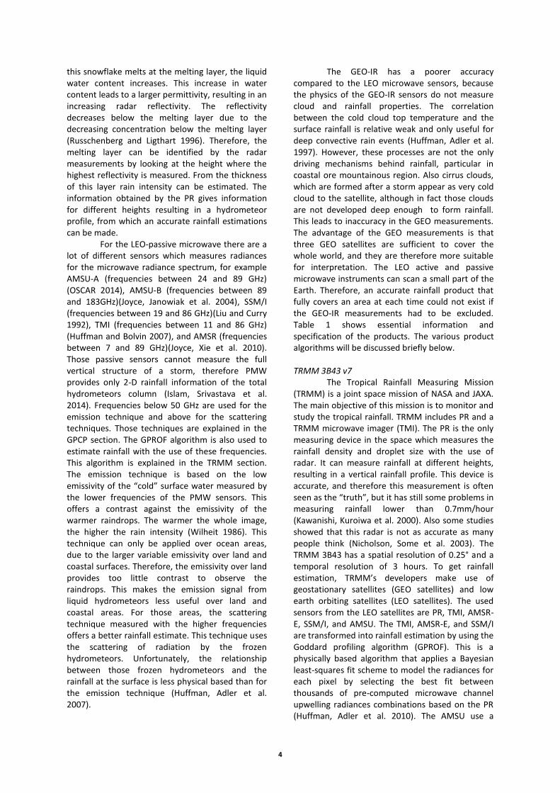
This research makes use of two different types of rainfall data, namely remote sensed gridded rainfall products and rain gauge point measurements. The open access rainfall products that are compared and validated in this research are: TRMM 3B43, GPCP V2.2, GPCP1DD, CRU TS3.21, ERA-interim, ARC 2.0, CHIRPS v1.8, RFE 2.0, PERSIANN, CMORPH, GSMaP_MVK, TAMSAT, and GPCC. These products use different combinations of specific spectral radiance measurements. The spatially distributed rainfall products can be divided into 3 main categories, namely the model based (ECMWF), ground based (CRU TS3.21 and GPCC), and the satellite based products. The used input data for each product is shown in Table 2.

The spectral radiometers onboard of the geostationary (GEO) satellites such as GOES and Meteosat can be divided into 3 different classes of sensors: GEO-VIS, GEO-NIR, and the GEO-TIR. The GEO-VIS (frequencies between 430 and 790 THz) uses the visible part of the light spectrum resulting in an imagery which could also be seen with the human eyes. This can be used to estimate the thickness of the clouds which could provide useful information about the type of clouds, but the image hardly gives information about the rain intensities.

Furthermore, this information is only useful during daytime. The GEO-NIR (frequencies between 100 and 400 THz) gives information on the properties of the cloud top particles. But also these channels are restricted to use only during daytime, because solar illumination is needed (Kidd, Levizzani et al. 2009). The last GEO sensor is the GEO-TIR (frequencies between 100 and 10 THz), which is also used for the rainfall algorithms and for Africa measured by the SEVIRI sensor onboard the Meteosat satellites. This sensor gives useful information for day and night time, which contains information about the temperature of the cloud top (Kidd, Levizzani et al. 2009). In the remaining of this paper those measurements are called GEO-IR measurements. The sensors onboard of the low earth orbit (LEO) satellites such as NOAA, DMSP, METOP, and TRMM, can be divided into LEO-active microwave and LEO-passive microwave. The Precipitation Radar (PR) is an example of an active microwave sensor which is onboard of the TRMM satellite and emits and measures the 13.8GHz frequency (Kozu, Kawanishi et al. 2001). This frequency is reflected by water particles and gives insight information on the intensity and distribution of rain, the rain type, and on the melting layer. The melting layer can give more insight in the type of storm. This layer can be found by looking at the reflectivity over the height measured with the PR. In the top of a cloud snowflakes are reflecting the radar signal, but when

Figure 1: (A) the average yearly rainfall measured with TRMM3B43 and averaged over 2000 till 2010 and (B) the sub basins of the Nile Basin.

4

this snowflake melts at the melting layer, the liquid water content increases. This increase in water content leads to a larger permittivity, resulting in an increasing radar reflectivity. The reflectivity decreases below the melting layer due to the decreasing concentration below the melting layer (Russchenberg and Ligthart 1996). Therefore, the melting layer can be identified by the radar measurements by looking at the height where the highest reflectivity is measured. From the thickness of this layer rain intensity can be estimated. The information obtained by the PR gives information for different heights resulting in a hydrometeor profile, from which an accurate rainfall estimations can be made.

For the LEO-passive microwave there are a lot of different sensors which measures radiances for the microwave radiance spectrum, for example AMSU-A (frequencies between 24 and 89 GHz) (OSCAR 2014), AMSU-B (frequencies between 89 and 183GHz)(Joyce, Janowiak et al. 2004), SSM/I (frequencies between 19 and 86 GHz)(Liu and Curry 1992), TMI (frequencies between 11 and 86 GHz) (Huffman and Bolvin 2007), and AMSR (frequencies between 7 and 89 GHz)(Joyce, Xie et al. 2010). Those passive sensors cannot measure the full vertical structure of a storm, therefore PMW provides only 2-D rainfall information of the total hydrometeors column (Islam, Srivastava et al. 2014). Frequencies below 50 GHz are used for the emission technique and above for the scattering techniques. Those techniques are explained in the GPCP section. The GPROF algorithm is also used to estimate rainfall with the use of these frequencies. This algorithm is explained in the TRMM section. The emission technique is based on the low emissivity of the “cold” surface water measured by the lower frequencies of the PMW sensors. This offers a contrast against the emissivity of the warmer raindrops. The warmer the whole image, the higher the rain intensity (Wilheit 1986). This technique can only be applied over ocean areas, due to the larger variable emissivity over land and coastal surfaces. Therefore, the emissivity over land provides too little contrast to observe the raindrops. This makes the emission signal from liquid hydrometeors less useful over land and coastal areas. For those areas, the scattering technique measured with the higher frequencies offers a better rainfall estimate. This technique uses the scattering of radiation by the frozen hydrometeors. Unfortunately, the relationship between those frozen hydrometeors and the rainfall at the surface is less physical based than for the emission technique (Huffman, Adler et al. 2007).

The GEO-IR has a poorer accuracy compared to the LEO microwave sensors, because the physics of the GEO-IR sensors do not measure cloud and rainfall properties. The correlation between the cold cloud top temperature and the surface rainfall is relative weak and only useful for deep convective rain events (Huffman, Adler et al. 1997). However, these processes are not the only driving mechanisms behind rainfall, particular in coastal ore mountainous region. Also cirrus clouds, which are formed after a storm appear as very cold cloud to the satellite, although in fact those clouds are not developed deep enough to form rainfall. This leads to inaccuracy in the GEO measurements. The advantage of the GEO measurements is that three GEO satellites are sufficient to cover the whole world, and they are therefore more suitable for interpretation. The LEO active and passive microwave instruments can scan a small part of the Earth. Therefore, an accurate rainfall product that fully covers an area at each time could not exist if the GEO-IR measurements had to be excluded. Table 1 shows essential information and specification of the products. The various product algorithms will be discussed briefly below. TRMM 3B43 v7

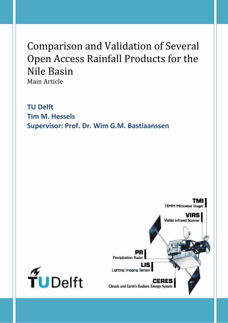
The Tropical Rainfall Measuring Mission (TRMM) is a joint space mission of NASA and JAXA. The main objective of this mission is to monitor and study the tropical rainfall. TRMM includes PR and a TRMM microwave imager (TMI). The PR is the only measuring device in the space which measures the rainfall density and droplet size with the use of radar. It can measure rainfall at different heights, resulting in a vertical rainfall profile. This device is accurate, and therefore this measurement is often seen as the “truth”, but it has still some problems in measuring rainfall lower than 0.7mm/hour (Kawanishi, Kuroiwa et al. 2000). Also some studies showed that this radar is not as accurate as many people think (Nicholson, Some et al. 2003). The TRMM 3B43 has a spatial resolution of 0.25° and a temporal resolution of 3 hours. To get rainfall estimation, TRMM’s developers make use of geostationary satellites (GEO satellites) and low earth orbiting satellites (LEO satellites). The used sensors from the LEO satellites are PR, TMI, AMSR-E, SSM/I, and AMSU. The TMI, AMSR-E, and SSM/I are transformed into rainfall estimation by using the Goddard profiling algorithm (GPROF). This is a physically based algorithm that applies a Bayesian least-squares fit scheme to model the radiances for each pixel by selecting the best fit between thousands of pre-computed microwave channel upwelling radiances combinations based on the PR (Huffman, Adler et al. 2010). The AMSU use a

5

scattering and emission technique developed by the National Environmental Satellite Data and Information Service (NESDIS) to transform the radiances into a precipitation amount. All the LEO precipitation estimates are merged into one product. Due the fact that the LEO satellites cannot cover the whole area, the gaps are filled with rainfall estimations based on GEO satellites. The GEO satellites are converted into rainfall estimations by using a Variable Rainrate (VAR) algorithm, which is based on the simple principle that colder clouds contain more precipitable water. To merge the LEO and the GEO rainfall estimations, the TRMM product uses a multi-satellite precipitation analysis (TMPA), which includes also ground measurements provided by Global Precipitation Climatology Center (GPCC). More information can be found in Huffman and Bolvin (2007) and on www.trmm.gsfc.nasa.gov. GPCP V2.2

The Global Precipitation Climatology Project (GPCP) is a rainfall dataset from 1979 until present on a 2.5° spatial grid and is developed by the World Climate Research Programme (WCRP). The product combines IR sensors from GEO satellites with SSM/I sensors from the LEO satellites. To calculate a rain rate from the SSM/I sensor, the emission algorithm (Wilheit, Chang et al. 1991) and the scattering algorithm (Grody 1991) are used. The emission technique utilize the emission of the rain clouds, this technique is more accurate than the scattering technique because they are more directly related to precipitation since the thermal radiation that is emitted from liquid hydrometeors is sensed directly (Joyce, Xie et al. 2010). The disadvantage is that the emission algorithm is only reliable above oceans, because the surface emissivity of the sea is low and uniform. Over land the scattering technique is more valuable. This is an 85GHz based technique which use the upwelling radiant energy that is scattered by the ice hydrometeors. The sensors detect the scattering of the upwelling radiation by precipitation sized ice particles within the rain layer. The technique calculates the scattering index, which is defined as the difference between in 85 GHz brightness temperature estimated from data at the lower frequency (19 and 22 GHz) channels and the observed one (Cheema 2012). This has a strong correlation with the surface rainfall (Huffman, Adler et al. 1997). The algorithm is calibrated with ground based radar estimations and can detect rain rates higher than 1mm/hour (Adler, Huffman et al. 2003). For the IR measurements the GOES Precipitation Index (GPI) technique is used (Arkin and Meisner 1987). This technique assigns a rainfall rate to every pixel with

a temperature colder than 235K a rain rate of 3mm/hour. With the SSM/I rain estimation, the GPI values can be adjusted (AGPI). The most closely corresponding SSM/I rainfall values are used to determine the ratio between the GPI and the SSM/I. This will result in adjusted spatially varying coefficients which are applied to the full set of GPI estimates. The last step is using the rain gauge data collected by the GPCC to reduce the bias. GPCP 1DD

Another product developed by the WCRP is the GPCP 1DD. 1DD stands for 1 degree daily which reveals the time and spatial resolution of the product. The same data is used as GPCP, but for this product the GPROF algorithm, also used for TRMM, is used to transfer the SSM/I measurements into a rain rate. To get a merged rainfall product a Threshold-Matched Precipitation Index (TMPI) is used. This algorithm allows the threshold and the rain rate values to vary monthly. The values are derived following the probability matching concepts (Kummerow and Giglio 1995). In this concept, monthly GEO IR histograms are derived from 3 hourly 1° GEO sensors and are matched with the SSM/I based frequency of precipitation. The threshold value is found by summing the bins with the lowest brightness temperature of the GEO IR histogram until the cumulative fraction of total pixels matches the SSM/I based fractional coverage (Huffman, Adler et al. 2001). The rain rate is determined by dividing the rain rate of the GPCP satellite/gauge product by the fractional occurrence of rain measured with the GEO IR. CRU TS3.21

The Climatic Research Unit Timeseries (CRU TS) produces monthly rainfall datasets on a 0.5° spatial resolution. Solely in-situ measurements from several databases are used. The databases that are used are Monthly Climatic Data for the World (MCDW), World Weather Records (WWR), and the CLIMAT. The CRU uses a Climate Anomaly Method (CAM) which means that anomalies are calculated from a base period. The base period is the long term monthly average from 1961 till 1990. The gauge data are converted to anomalies by subtracting the base period for that particular station (Harris, Jones et al. 2013). Hereafter, the anomalies are extrapolated within the correlation decay distance which is 450 kilometres for monthly precipitation. Surfaces that are not covered by the correlation decay distance use dummies stations with zero anomalies (Mitchell and Jones 2005). To make a grid, a triangulated linear interpolation is used to convert the rainfall in gridded values.

6

ERA-interim The ERA-interim product is developed by

the European Centre for Medium-Range Weather Forecasts (ECMWF). The ERA-interim use a physically based model, which is an atmospheric model and data assimilation system which is called the Integrated Forecast System (IFS). The model consist of three fully coupled components, namely atmosphere, land surface and ocean waves. The input for the model can be all kinds of observations, for example buoys, ships measurements, aircraft measurement, radiosonde, dropsonde, but also satellite measurements from the LEO and GEO satellites. The model equations make it possible to extrapolate the information from locally observed parameters to unobserved parameters in a physically meaningful way. Those parameters can be extrapolated forwards in time (Dee, Uppala et al. 2011). The initial conditions are produced with the use of data assimilation which calculates the best possible atmospheric state using the observations from satellites and in –situ data and the short range forecast provided by the previous model forecast. This input data are processed in space and time by a four-dimensional variation assimilation system (4D-VAR). In this process the observations are combined by calculating a weighted average based on a flow dependent structure function (Thépaut, Courtier et al. 1996). The model calculates precipitation based on the modelled temperature, wind and humidity information for a 0.75° grid. RFE 2.0

The Famine Early Warning System Network (FEWS NET) has developed the African Rainfall Estimation Algorithm Version 2 (RFE 2.0), which has a special resolution of 0.1° on hourly basis. RFE 2.0 is a merging technique of LEO and GEO measurements which has been shown to have an increasing accuracy of rainfall estimates (Xie and Arkin 1996). Also GPCC is used to reduce the bias of the product. The LEO sensors that are used are the SSM/I and the AMSU sensors. The scattering technique and emission techniques are used to obtain a rain rate (Ferraro and Marks 1995). GPI is used to convert GEO measurements into rainfall estimates. To merge the LEO and GEO rainfall estimates, a two step merging process is used. The first step is to reduce the random errors of all the satellite sources. Therefore, a maximum-likelihood estimation method is used to determine the weighting coefficients between the rainfall estimates. For this method, the GPCC is used as standard references over the land areas and atoll gauge precipitation observations of Morrissey and Greene (1991) over the oceanic areas. With the use of this reference the root-mean difference is

calculated. The second step is to compare the merge satellite precipitation estimate with the GPCC rain gauge data set to remove the bias. The precipitation will maintain the shape of the combined satellite precipitation estimates, but the magnitude is inferred from the GPCC dataset. This is especially the case in the direct surrounding of the GPCC rain station. If the distance increases, the rainfall estimates will rely more on the combined satellite product (NOAA 2001). ARC 2.0

Another product of FEWS NET is the Africa Rainfall Climatology (ARC 2.0) product, which has the same spatial and temporal resolution. A research showed that by using only the GPI and GPCC products of the RFE 2.0, one can improve the bias of the product while the correlation is just slightly lower (Love, Kumar et al. 2004). The same algorithms are used as RFE 2.0 (Novella and Thiaw 2013). CHIRPS v1.8

The Climate Hazards Group (CHG) developed the Climate Hazards Group IR Precipitation Station (CHIRPS) product. This product is a third generation precipitation procedure based on various interpolation schemes to create spatially continuous grids from raw point data (Funk, Husak et al. 2007). The CHIRPS uses the monthly precipitation climatology (CHPClim), the IR sensors from the GEO satellites, the TRMM 3B42 product, and the ground precipitation observations. The CHPClim is a high resolution global gridded and monthly precipitation averages with the monthly means for the period 1980 till present. The inputs of those maps are climate, satellite and topographic data to develop accurate and unbiased rainfall maps for each pentad (Funk, Michaelsen et al. 2011). The climate inputs are the station observations from GHCN, FAO, and GTS. The RFE 2.0 and GEO IR measurements are used as satellite input and the USGS HYDRO1K is used to get the slope and elevation as topographic input. The result is a 0.05° gridded map with long term mean rainfall for each pentad. This map is multiplied by the IR precipitation (IRP). Furthermore, a linear relation between rain rate and cold cloud duration (CCD) is assumed which is measured by the GEO IR. The constants parameters of this relation are defined by calibrating with the use of the TRMM 3B42 data. This linear relation is called the IR precipitation (IRP). Also the long term IRP is calculated for each pentad, which uses the data from 1981 till present. An unitless value is calculated by dividing the IRP by the long term IRP. This value is multiplied by the CHPClim to get the CHIRP product. Finally, the

7

CHIRP map uses the station observations to reduce the bias resulting in the CHIRPS product (Funk, Peterson et al. 2013). PERSIANN

University of California developed the Precipitation Estimation from Remotely Sensed Information Using Artificial Neural Networks (PERSIANN). The spatial resolution is 0.25° and the temporal resolution is 30 minutes. The only inputs are the TMI dataset from the TRMM satellite and the GEO IR dataset. Six parameters which can be defined from the GEO IR dataset are used as input for an Artificial Neural Network model. This model exists of two layers. The first layer is the Self Organizing Feature Map (SOFM) which transfers the IR input into the hidden layers (Kohonen 1982). The SOFM is used to classify the variables into a large number of groups associated with different cloud surface characteristics (Sorooshian, Hsu et al. 2000). The second layer is the Modified Grossberg Linear Layer (MGLL). This transfers the hidden layer into the output layer (Grossberg 1969). This component estimates the specific rainfall rate for each input pattern that is classified by the SOFM. The MGLL component and SOFM component are trained separately. The MGLL component is calibrated and updated by using the TMI (Hsu, Gao et al. 1997). CMORPH

Climate Prediction Center (CPC) morphing method (CMORPH) is developed by CPC. The idea of the product is to develop a merged GEO and LEO satellite product with the desirable aspect of the accuracy of the Leo satellites and the spatial and temporal coverage of the IR data. First, the rainfall estimates are produces with the use of the TMI sensor transferred with the GPROF algorithm and with the use of the SSM/I, AMSR and AMSU sensor transferred with the NESDIS algorithm. The GEO IR is used to make a cloud system advection vector map (CSAV). This map is used to propagate and morph the LEO rain rate estimations in time (Joyce, Janowiak et al. 2004). The result is a rainfall estimation product on a 0.25° grid every 3 hours. GSMaP_MVK

The Global Satellite Mapping of Precipitation (GSMaP) developed by JAXA estimates precipitation with an hourly resolution for a 0.1° grid. This product use two morphing techniques from the moving vector obtained from the IR images and a Kalman Filter. The Kalman filter tries to estimate the state of a process from a series of noisy measurements. The series of noisy measurements is obtained from the IR images. Those measurements are statistically correlated

with the surface precipitations rate, but have large variances. Research shows that the variation of precipitation rate in 1 hour is normally distributed with zero mean when one compare the propagated rain rate forward in time with the precipitation rate retrieved from the microwave sensor (Ushio, Sasashige et al. 2009). This enables the application of the Kalman filter theory. The Kalman gain is computed to refine the precipitation rate after its propagation (Ushio and Kachi 2010). The GEO IR measurements are used to calculate cloud motion vectors and the previous output of GSMaP_MVK is morphed with the use of this cloud motion vector map. Hereafter the Kalman Filter is applied. The TMI, SSM/I, and AMSR from the LEO satellites are transferred into rainfall estimations by using scattering and emission techniques. To make a merged product the LEO satellite product has the priority. The gaps are filled with the precipitation map determine with the two morphing techniques (Kubota, Shige et al. 2007). TAMSAT

The University of Reading developed a rainfall estimate based on only GEO satellites and ground data. This product is called the Tropical Applications of Meteorology using Satellite data and ground based observations (TAMSAT). The principle of TAMSAT is based upon the Cold Cloud Duration (CCD). This is the total time that the temperature of the top of a cloud is below a certain threshold. This threshold temperature varies in space and month. Therefore, Africa is divided into geographical zones on basis of annual isohyets and similar climatic conditions within the zone (Thorne, Coakeley et al. 2001). With the use of a Contingency table between the ground observations and the CCD, the rain threshold is determined. The rainfall is estimated by assuming a linear regression between CCD and rain rate. The parameters for this regression line are calibrated with the use of historic rain gauge and CCD (Grimes, Pardo-Iguzquiza et al. 1999). GPCC

The Global Precipitation Climatology Centre (GPCC) is developed by die Deutcher Wetterdienst (DWD). The full data product is based on 40.000 gauges, the exact amount depends on the quality of individual gauges and varies between 30.000 and 40.000 gauges. To calculate area means on a grid from point data, DWD uses the following steps. First the irregularly distributed gauge observations are interpolated into points of a regular grid. This is done by using an adapted version of SPHEREMAP (Shepard 1968). This interpolation method takes the distance of a station

8

to the grid point into account, the directional distribution of stations, and the gradients of the data field in the grid point environment. Hereafter, the area averaged precipitation is calculated as arithmetic mean from the four corners of the grid cell. 3.2 Ground products

For the validation of the open access rainfall products, raw ground point measurements are used. In total 62 ground stations are used. This also includes a dense network of 24 ground

measurements for the Blue Nile sub basin. The rest of the Nile Basin has a coarser network (see Figure 2). To overcome the mismatch problem between rain gauges and satellite-based gridded rainfall products, the point data is transferred into gridded data. The interpolation techniques will be discussed in section 3.4.

A disadvantage of these interpolation techniques are the sampling errors which will be introduced in the “truth”. Therefore, comparing grid to pixels was also performed. These results were very difficult to interpret, due to the large

Table 1: Summary of the different satellite products

Product Developer Spatial resolution

Covering area Temporal resolution

Time span Ground measurement

TRMM 3B43 v7 NASA, JAXA 0.25° 0°E-360°E/50°N-50°S 3 hourly Jan 1998 - present Yes

GPCP V2.2 WCRP (GEWEX)

2.5° 0°E-360°E/90°N-90°S Monthly Jul 1987 - present Yes

GPCP1DD WCRP (GEWEX)

1° 0°E-360°E/90°N-90°S Daily Oct 1996 - present Yes

CRU TS3.21 University of East Anglia

0.5° 0°E-360°E/90°N-90°S Monthly Jan 1901 - present Yes

ERA-interim ECMWF 0.75° 0°E-360°E/90°N-90°S 6 Hourly Jan 1979 - present Yes

RFE 2.0 NOAA (CPC) 0.1° 20°E-55°E/40°N-40°S Hourly Jan 2001 - present Yes

ARC 2.0 NOAA (CPC) 0.1° 20°E-55°E/40°N-40°S Hourly Jan 1983 - present Yes

CHIRPS v1.8 CHG 0.05° 0°E-360°E/50°N-50°S Pentads (Daily for Africa)

Jan 1983 - present Yes

PERSIANN University of California

0.25° 0°E-360°E/60°N-60°S 30 minutes Mar 2000 - present No

CMORPH NOAA (CPC) 0.25° 0°E-360°E/60°N-60°S 3 Hourly Dec 2002 - present No

GSMaP_MVK JAXA (JST) 0.1° 0°E-360°E/60°N-60°S Hourly May 2000 - present No

TAMSAT University of Reading

0.0375° Africa Decadal Jan 1983 - present Yes

GPCC DWD 0.5° 0°E-360°E/90°N-90°S Monthly Jan 1901 - present Yes

Table 2: Summary of the used input sensor of the different satellite products

Sensors TRM

M

3B

43

CM

OR

PH

GP

CP

GP

CP

1D

D

PER

SIAN

N

GSM

aP

RFE 2.0

AR

C 2

.0

CH

IRP

S

ERA

-

inte

rim

CR

U

TAM

SAT

GP

CC

GEO

SEVIRI

LEO

x

x

x

x

x

x

x

x

x

x

x

Precipitation Radar x

AMSU x x x x x

SSMI x x x x x x x

TMI x x x x x

AMSR

x x x x

Rainfall Measurements

Ground Measurements

x

x

x

x

x

x

x

x

x

x

Rainfall Products

TRMM 3B42 x

RFE 2.0 x

9

differences in correlations that were found between the different ground measurements and satellite products. Even the products correlations of neighbouring stations were showing large differences between each other. These large differences are a result of comparing the grid averaged rainfall measured by the satellite with the exact rainfall measured by the ground station. This comparison between average rainfall and exact rainfall leads only into a good correlation for ground gauges which measurements approaches the areal averages. This made it very difficult to validate the rainfall products based on this comparison. By interpolating these point measurements into average grid rainfall, will make the ground measurements better comparable with the satellite products despite of the introduced sampling errors. Furthermore, WA+ needs gridded data as input, therefore validation on a grid resolution is more useful for WA+ purposes than on a point resolution.

The error introduced in the “truth” due to the interpolation technique is equal for all the

products, therefore the validation can still be performed. But the calculated errors are not only caused by the product, but also due to this introduced sampling error inside the “truth”. This has to be kept in mind.

Table 3 shows the location and the name of the ground stations that are involved in this research. Some of those stations are probably also involved in the GPCC products, but it is impossible to know which station is exactly involved the gauges that are used for the GPCC analysis are not identified (Nicholson, Some et al. 2003). Therefore, the problem arises whether the ground measurements used for the validation are completely independent compared to the rainfall satellite products. Nine out of the 13 products specify that ground measurements are used for the calibration (see Table 1). Therefore, a distinction is made between the rainfall products which bias is not reduced (CMORPH, PERSIANN and GSMaP_MVK) and the products that have a reduced bias with the use of ground measurements.

Table 3: Position of the ground measurements used in the validation

Name Latitude Longitude Name Latitude Longitude

Sennar 13.33 33.37 Wereta 11.92 37.68 Rashad 11.52 31.03 Zege 11.68 37.32 Obied 13.10 30.14 Maksegnit 12.37 37.55 Nyala 12.03 24.53 Kidmaja 11.00 36.80 Nahoud 12.42 28.26 Kimbaba 11.55 37.38 Madini 14.24 33.29 Wetetabay 11.37 37.05 Kosti 13.10 32.40 Gundil 10.95 37.07 Khar 15.60 32.55 Abay Sheleko 11.38 36.87 Kasala 15.28 36.24 Urana 10.89 36.86 Kadugli 11.00 29.43 Wau 7.42 28.01 Atbara 17.42 33.58 Malakal 9.22 31.39 Gadarf 14.02 35.24 Juba 4.52 31.36 Fasher 13.37 25.20 Yetemen 10.33 38.13 Duem 14.00 32.20 Shindi 10.43 36.57 Damazine 11.47 34.23 Debre Marcos 10.21 37.43 Babanusa 11.20 27.49 Teppi 7.2 35.42 Gonder 12.32 37.26 Masha 7.73 35.48 Asswan 23.58 32.47 Assosa 10.02 34.32 Cairo 30.08 31.24 Begi 9.35 34.53 Luxor 25.40 32.42 Sekela 11.00 37.13 Qena 26.20 32.75 Motta 10.08 37.87 Asyout 27.03 31.01 Finote 11.41 37.16 El Minya 28.05 30.44 Gebeya 9.20 39.38 Dangla 11.12 36.42 Kitala 1.02 35.00 Debre Tabor 11.88 38.03 El Doret 0.41 35.22 Addizemen 12.12 37.87 Kisumu -0.10 34.75 Ayikel 12.53 37.05 Bukoba -1.33 31.82 Adet 11.27 37.47 Musoma -1.50 33.80 Gorgora 12.25 37.30 Mwanza -2.47 32.92 Enjibara 11.00 37.00 Kigoma -4.88 29.63 Enfraz 11.18 37.68 Kigali -1.96 30.13

10

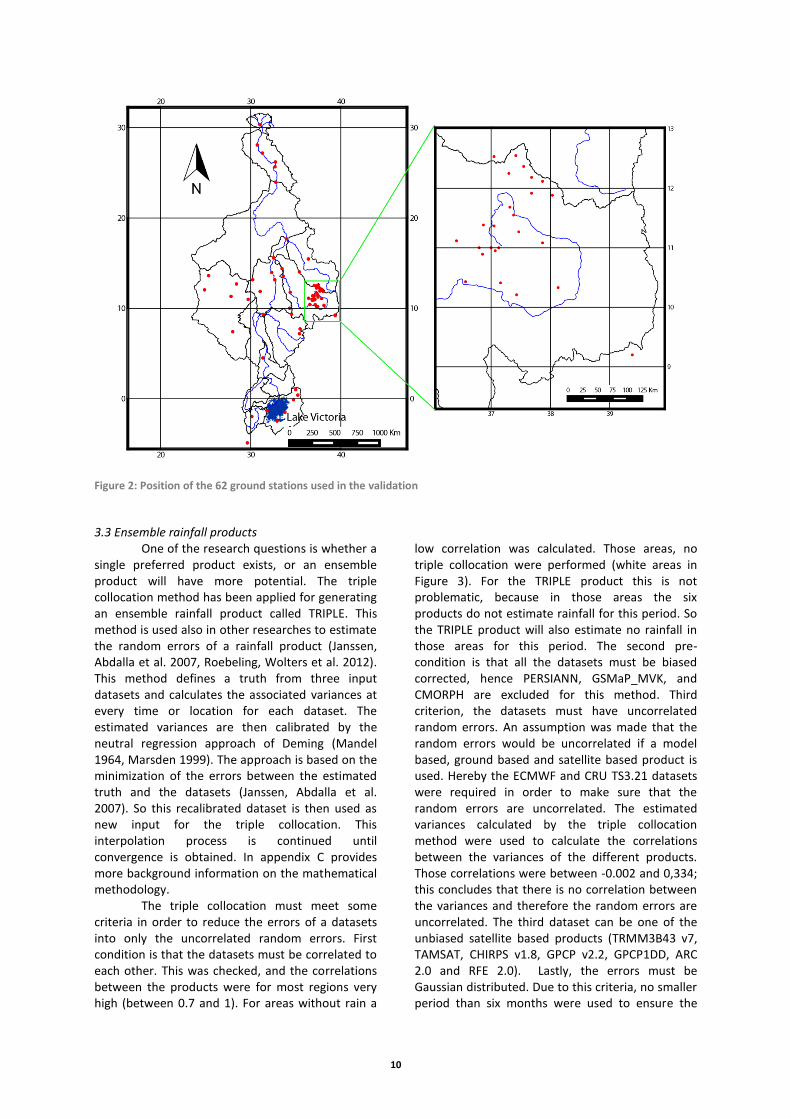
3.3 Ensemble rainfall products

One of the research questions is whether a single preferred product exists, or an ensemble product will have more potential. The triple collocation method has been applied for generating an ensemble rainfall product called TRIPLE. This method is used also in other researches to estimate the random errors of a rainfall product (Janssen, Abdalla et al. 2007, Roebeling, Wolters et al. 2012). This method defines a truth from three input datasets and calculates the associated variances at every time or location for each dataset. The estimated variances are then calibrated by the neutral regression approach of Deming (Mandel 1964, Marsden 1999). The approach is based on the minimization of the errors between the estimated truth and the datasets (Janssen, Abdalla et al. 2007). So this recalibrated dataset is then used as new input for the triple collocation. This interpolation process is continued until convergence is obtained. In appendix C provides more background information on the mathematical methodology.

The triple collocation must meet some criteria in order to reduce the errors of a datasets into only the uncorrelated random errors. First condition is that the datasets must be correlated to each other. This was checked, and the correlations between the products were for most regions very high (between 0.7 and 1). For areas without rain a

low correlation was calculated. Those areas, no triple collocation were performed (white areas in Figure 3). For the TRIPLE product this is not problematic, because in those areas the six products do not estimate rainfall for this period. So the TRIPLE product will also estimate no rainfall in those areas for this period. The second pre-condition is that all the datasets must be biased corrected, hence PERSIANN, GSMaP_MVK, and CMORPH are excluded for this method. Third criterion, the datasets must have uncorrelated random errors. An assumption was made that the random errors would be uncorrelated if a model based, ground based and satellite based product is used. Hereby the ECMWF and CRU TS3.21 datasets were required in order to make sure that the random errors are uncorrelated. The estimated variances calculated by the triple collocation method were used to calculate the correlations between the variances of the different products. Those correlations were between -0.002 and 0,334; this concludes that there is no correlation between the variances and therefore the random errors are uncorrelated. The third dataset can be one of the unbiased satellite based products (TRMM3B43 v7, TAMSAT, CHIRPS v1.8, GPCP v2.2, GPCP1DD, ARC 2.0 and RFE 2.0). Lastly, the errors must be Gaussian distributed. Due to this criteria, no smaller period than six months were used to ensure the

Figure 2: Position of the 62 ground stations used in the validation

11

Gaussian distribution of errors, so 66 rainfall estimations (6 months times 11 years) were assumed to give a Gaussian distribution of errors.

The triple collocation method is performed on a 0.75° grid resolution, the finest possible grid due to the model based product which must be included. When the calculations were done on a finer grid, a sampling error in the ECMWF dataset will be introduced due to the performed interpolation technique. Therefore, the triple collocation method is performed on the coarsest grid of the three input dataset. Whereby, the sampling error can be reduced which will lead in a better random error estimation calculated by this method. Satellite products coarser than 0.75° were not used, otherwise the triple collocation had to be performed on a coarser grid.

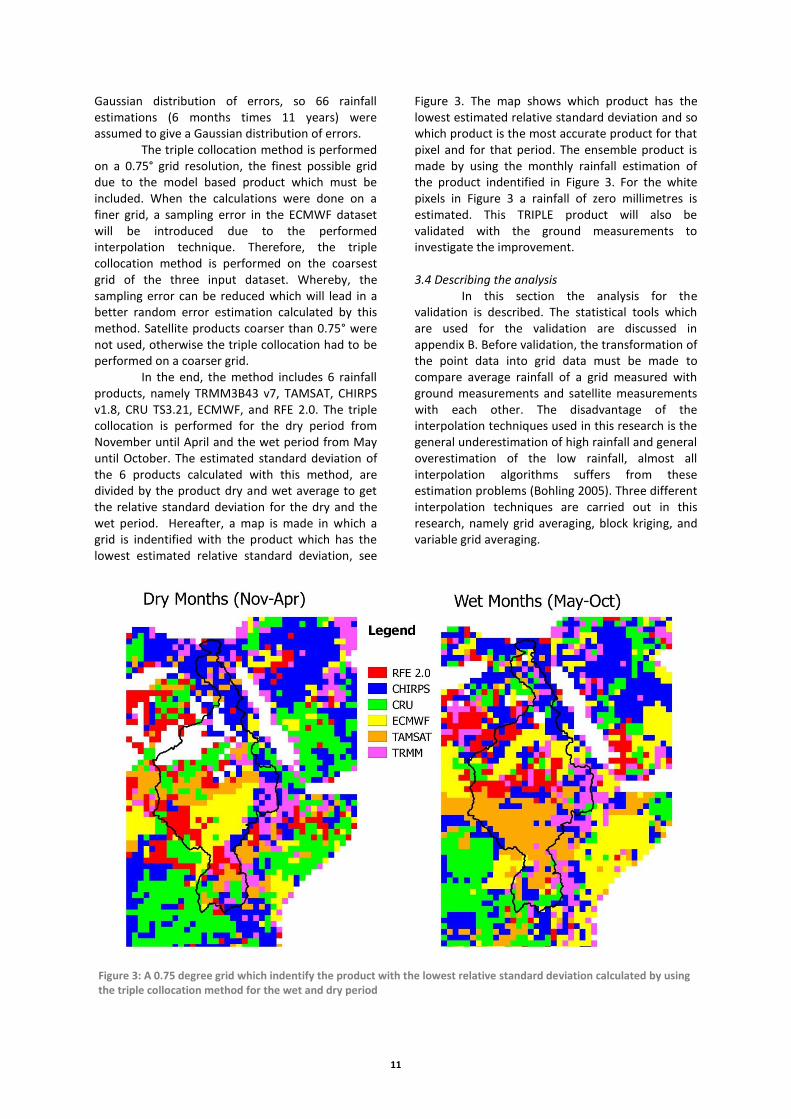
In the end, the method includes 6 rainfall products, namely TRMM3B43 v7, TAMSAT, CHIRPS v1.8, CRU TS3.21, ECMWF, and RFE 2.0. The triple collocation is performed for the dry period from November until April and the wet period from May until October. The estimated standard deviation of the 6 products calculated with this method, are divided by the product dry and wet average to get the relative standard deviation for the dry and the wet period. Hereafter, a map is made in which a grid is indentified with the product which has the lowest estimated relative standard deviation, see

Figure 3. The map shows which product has the lowest estimated relative standard deviation and so which product is the most accurate product for that pixel and for that period. The ensemble product is made by using the monthly rainfall estimation of the product indentified in Figure 3. For the white pixels in Figure 3 a rainfall of zero millimetres is estimated. This TRIPLE product will also be validated with the ground measurements to investigate the improvement. 3.4 Describing the analysis

In this section the analysis for the validation is described. The statistical tools which are used for the validation are discussed in appendix B. Before validation, the transformation of the point data into grid data must be made to compare average rainfall of a grid measured with ground measurements and satellite measurements with each other. The disadvantage of the interpolation techniques used in this research is the general underestimation of high rainfall and general overestimation of the low rainfall, almost all interpolation algorithms suffers from these estimation problems (Bohling 2005). Three different interpolation techniques are carried out in this research, namely grid averaging, block kriging, and variable grid averaging.

Figure 3: A 0.75 degree grid which indentify the product with the lowest relative standard deviation calculated by using the triple collocation method for the wet and dry period

12

For the grid averaging technique, a grid is

projected upon the observed data points. For each grid, rainfall estimates are calculated by averaging all the point rainfall data that are located inside the projected grid. The advantage is that this method is very simple and straight forward, but the disadvantage is that for some grids the rainfall estimate only results from one measuring point. This will result in a large sampling error of the rainfall estimate. This is specially the case for the validations done on a larger grid size.

Block kriging is a more sophisticated method to transfer point data into gridded rainfall estimates. The first step in this method is fitting semivariograms from the monthly ground rainfall data points. Those semivariogram gives the relation between the variance and the distance between the measurements. A Gaussian, spherical and exponential curve is fitted through this relation and the fit with the lowest root mean squared error is taken as semivariogram. This semivariogram is different for every month and for every ground measurement point. With the use of this semivariogram the correlation can be found, which is used in the interpolation method. Instead of averaging only the points located inside the grid, what is done in the grid averaging method, this method uses all the data points with a certain weight. This weight depends on the correlation between the point and the grid and the correlation between the points. The advantage of block kriging is that it helps to compensate the clustering effect of data points and block kriging gives and estimation of the error. This estimate error is used to calculate the coefficient of variation (standard deviation divided by the mean) of the estimated “truth”, so one can define how accurate the “truth” is. The disadvantage is that it requires more calculating time than the other two methods and can be felt as difficult to comprehend (Vogelzang and Stoffelen 2012).

The last method is a method based on a variable grid. This variable grid can have every size between a maximum of 5 degrees and a minimum of 0.25 degrees. The only requirement for the grid is that an amount of five ground gauges must be enclosed inside the grid. The average of the five ground measurements will give a good estimation of the rainfall of that grid. When a 2.5 degree grid is used which includes 5 ground measurements an error of 10% can be attained (Xie and Arkin 1995). In this method a maximum grid size of 5 degrees is used, otherwise only grids in the Blue Nile will be formed. For the Blue Nile the grids are smaller due

to the higher station concentration, which lead to a lower sampling error. While in the other parts the formed grids are larger, whereas the rainfall patterns are less complex, which will also result in a lower sampling error. 4. Comparison of the open access rainfall products

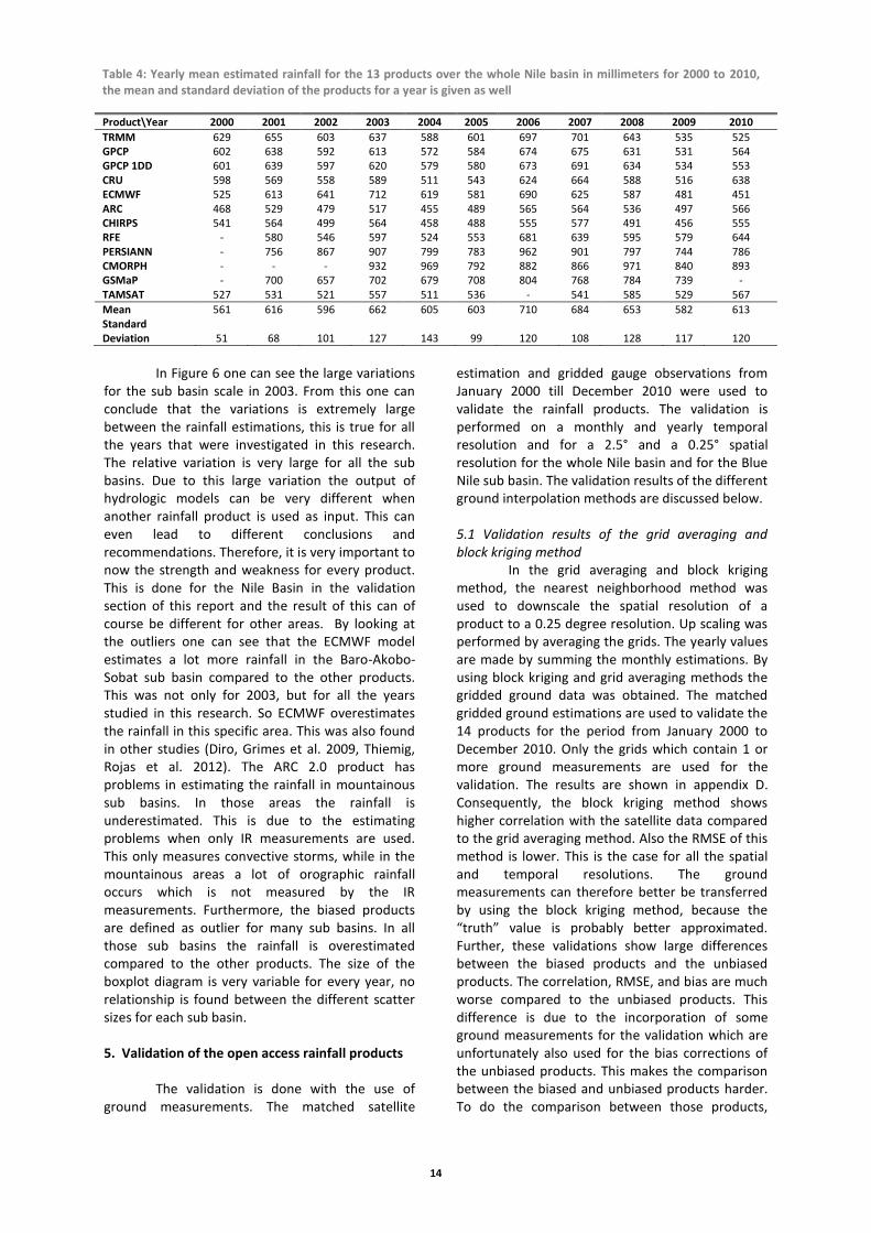
The yearly average rainfall for the Nile Basin are made by calculating the average rainfall of each product over a 0.1 degree gridded mask which contains the whole Nile basin, the products with a coarser grid were interpolated with the use of the nearest neighbour method. The yearly averages over the whole Nile basin for the 13 products are shown in Table 4. By comparing the average rainfall of the Nile basin over the year, one can see that the differences between the estimations of the products are large, see also Figure 4. The products that were not unbiased (PERSIANN, CMORPH and GSMaP_MVK) show larger rainfall estimation than the other products. The standard deviation between the products in 2002 to 2010 is double the amount compared to the standard deviation in 2000 (see Table 4), this is due to the inclusion of the three biased rainfall products from 2002 to 2010. ARC 2.0, TAMSAT and CHIRPS v1.8 show the lowest amount of rainfall estimation. This is true for a mean, dry and a wet year. ARC 2.0 and TAMSAT are products that use merely IR measurements, CHIRPS v1.8 use also only IR measurements, but it also uses the TRMM3B42 v7 to calibrate the IR measurements and it use the long period climate map (CHPClim) which is among other things based on the RFE 2.0. It seems that those products estimate lower rainfall then the other products which also use PMW measurements directly.

A boxplot diagram is made of the relative anomalies of the products between 2003 and 2010. The results for the wet months are shown in Figure 5. GSMaP and TAMSAT show small variations over the years during the wet months. TRMM3B43 v7, GPCP, GPCP1DD, CRU TS3.21 and GPCC show similar variations over the years. This is probably due to the bias correction. The correction of those products is done with the GPCC dataset. Therefore, the variations over the years become similar for those datasets. Also RFE 2.0 and ARC 2.0 are bias corrected with GPCC, but those variations over the years are less similar. The biased products show in order of magnitude the same relative variations as the unbiased products, while those annual rainfall amounts are much higher compared to the unbiased products.

13

Figure 4: The mean annual rainfall over the Nile Basin measured by for the 14 products for the mean over 2003 and 2009, wet year, and a dry year.

Figure 5: The percentage of the anomalies for the whole Nile basin (between 2003 to 2010) of the different products showed in a boxplot diagram for the wet months. The bar in the box defines the median, the upper and lower side of the box indicate the 25

th and 75

th percentage. The plus signs indicate outliers which are defined above 1.5 times the

difference between the 25th

or 75th

percentage. The bars above the box show the highest and the lowest estimation without the outliers.

Figure 6: The variation of the 13 products for the different sub basins showed in a boxplot diagram for 2003, the bar in the box defines the median, the upper and lower side of the box indicate the 25

th and 75

th percentage. The plus signs

indicate outliers which are defined above 1.5 times the difference between the 25th

or 75th

percentage. The bars above the box show the highest and the lowest estimation without the outliers.

14

In Figure 6 one can see the large variations

for the sub basin scale in 2003. From this one can conclude that the variations is extremely large between the rainfall estimations, this is true for all the years that were investigated in this research. The relative variation is very large for all the sub basins. Due to this large variation the output of hydrologic models can be very different when another rainfall product is used as input. This can even lead to different conclusions and recommendations. Therefore, it is very important to now the strength and weakness for every product. This is done for the Nile Basin in the validation section of this report and the result of this can of course be different for other areas. By looking at the outliers one can see that the ECMWF model estimates a lot more rainfall in the Baro-Akobo-Sobat sub basin compared to the other products. This was not only for 2003, but for all the years studied in this research. So ECMWF overestimates the rainfall in this specific area. This was also found in other studies (Diro, Grimes et al. 2009, Thiemig, Rojas et al. 2012). The ARC 2.0 product has problems in estimating the rainfall in mountainous sub basins. In those areas the rainfall is underestimated. This is due to the estimating problems when only IR measurements are used. This only measures convective storms, while in the mountainous areas a lot of orographic rainfall occurs which is not measured by the IR measurements. Furthermore, the biased products are defined as outlier for many sub basins. In all those sub basins the rainfall is overestimated compared to the other products. The size of the boxplot diagram is very variable for every year, no relationship is found between the different scatter sizes for each sub basin. 5. Validation of the open access rainfall products

The validation is done with the use of

ground measurements. The matched satellite

estimation and gridded gauge observations from January 2000 till December 2010 were used to validate the rainfall products. The validation is performed on a monthly and yearly temporal resolution and for a 2.5° and a 0.25° spatial resolution for the whole Nile basin and for the Blue Nile sub basin. The validation results of the different ground interpolation methods are discussed below. 5.1 Validation results of the grid averaging and block kriging method

In the grid averaging and block kriging method, the nearest neighborhood method was used to downscale the spatial resolution of a product to a 0.25 degree resolution. Up scaling was performed by averaging the grids. The yearly values are made by summing the monthly estimations. By using block kriging and grid averaging methods the gridded ground data was obtained. The matched gridded ground estimations are used to validate the 14 products for the period from January 2000 to December 2010. Only the grids which contain 1 or more ground measurements are used for the validation. The results are shown in appendix D. Consequently, the block kriging method shows higher correlation with the satellite data compared to the grid averaging method. Also the RMSE of this method is lower. This is the case for all the spatial and temporal resolutions. The ground measurements can therefore better be transferred by using the block kriging method, because the “truth” value is probably better approximated. Further, these validations show large differences between the biased products and the unbiased products. The correlation, RMSE, and bias are much worse compared to the unbiased products. This difference is due to the incorporation of some ground measurements for the validation which are unfortunately also used for the bias corrections of the unbiased products. This makes the comparison between the biased and unbiased products harder. To do the comparison between those products,

Table 4: Yearly mean estimated rainfall for the 13 products over the whole Nile basin in millimeters for 2000 to 2010, the mean and standard deviation of the products for a year is given as well

Product\Year 2000 2001 2002 2003 2004 2005 2006 2007 2008 2009 2010

TRMM 629 655 603 637 588 601 697 701 643 535 525 GPCP 602 638 592 613 572 584 674 675 631 531 564 GPCP 1DD 601 639 597 620 579 580 673 691 634 534 553 CRU 598 569 558 589 511 543 624 664 588 516 638 ECMWF 525 613 641 712 619 581 690 625 587 481 451 ARC 468 529 479 517 455 489 565 564 536 497 566 CHIRPS 541 564 499 564 458 488 555 577 491 456 555 RFE - 580 546 597 524 553 681 639 595 579 644 PERSIANN - 756 867 907 799 783 962 901 797 744 786 CMORPH - - - 932 969 792 882 866 971 840 893 GSMaP - 700 657 702 679 708 804 768 784 739 - TAMSAT 527 531 521 557 511 536 - 541 585 529 567

Mean 561 616 596 662 605 603 710 684 653 582 613 Standard Deviation 51 68 101 127 143 99 120 108 128 117 120

15

more research is needed in the exact data that is used in the bias removal process, or obtain data which is surely not used for bias correcting. This is not done in this study.

When one compares the validation results of the Nile Basin and the Blue Nile, one can see that the correlation and RMSE is for most products a bit better. The bias is for all products lower, all the unbiased products underestimate the rainfall for the Blue Nile basin. This is probably due to the measurements errors of the IR measurements in mountainous areas. This is based on the cloud top temperature, but in areas with mountains this approach is less accurate to estimate rainfall. This is due to orographic lift which also causes rainfall, which cannot be measured by IR measurements. The products which include PMW in the estimation have a lower underestimation, for those products IR measurements are still needed to cover the whole world.

When the more local 0.25 degree grid is used, the RMSE increases. The estimated errors calculated in the block kriging method were used, to calculate the coefficient of variation which became much lower for the 0.25 degree situation. The coefficient was 0.35 for the 2.5 degree scale and 0.17 for the 0.25 degree scale. Thereby it can be assumed that the gridded ground measurements will approximate the “truth” more for a finer spatial resolution, but still this “truth” contains some errors. The satellite products have more difficulties in estimating the local rainfall leading to a higher RMSE.

On a yearly temporal resolution, the discrepancies between the ground estimations and the satellite estimations are smaller, leading to a lower RMSE. This is due to the reduced sampling error when a large timescale is used. For the monthly 0.25 degree validation the bias becomes more negative, this is due to the possibility to form more grids which includes a ground measurement for the Blue Nile. The rainfall in this mountainous area is underestimated by all the products, so when more grids are formed in this specific area the products get a more negative bias. 5.2 Validation results with the use of the variable grid averaging method

The last validation is with the use of variable grid sizes, see also appendix D. The maximum grid size is 5 degrees. The formed grid approaches the “truth” very well due to the 5 stations that are involved in the estimation.

When one compare this method to the other two methods. One can see that the correlations are a little higher and the RMSE is a little lower. This is because a couple of reasons.

Firstly, in all estimations a lot of ground measurements are involved. This makes the ground estimation more accurate. While for the other methods some pixels consist of just 1 ground measurement. Secondly, involving grids with a maximum of 5 degrees also leads to a better correlation, this is also visible when one compares the results of the different spatial resolutions of the block kriging method. The coarser spatial resolution has a higher correlation and a lower RMSE. One could also decrease the maximum grids size, but then only grids will be formed in the Blue Nile, because only this area has such a dense ground gauge network.

Compared with the other validation methods, the bias of the variable grid averaging method is more negative. This is also the result of the more dense ground gauge network for the Blue Nile region, therefore more grids can be formed in this specific area. From the other validation methods, it can already conclude that the Blue Nile basin has a larger negative bias compared to the bias of the total Nile Basin. So when more grids can be formed in the Blue Nile the total bias of the whole Nile Basin becomes also more negative. With this method, the Blue Nile sub basin becomes a very dominant area due to the dense ground network. 5.3 Discussion of the validation

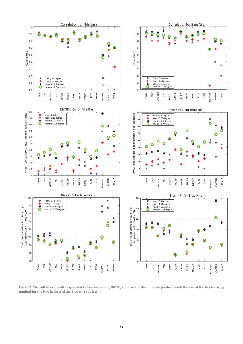
The results of the three validation methods are shown in Appendix D, the results for each product are discussed here. From all the methods the same conclusions can be drawn namely: biased products show a lower correlation compared to the unbiased products and the sequence between products of higher correlation is also the same. But if the different validation methods are compared, one can see that the block kriging method results in a higher correlation for all the products compared to the simple averaging method, so with this method a better relationship is obtained between the products and the ground measurements. The variable grid averaging method has the best correlation and RMSE, but this is also due to the conditions of having 5 measurements within a maximum of 5 degrees. When this conditions is lower a worse correlation and RMSE was founded. Also this method makes the Blue Nile basin very dominant due to the dense ground network, while the validation must be done for the whole Nile Basin. Therefore, the block kriging method is more favourable and this method will be used to compare the products results in the remaining of this section. The validation results of the block kriging method are visualized in Figure 7 in order to make the appendix D more visual. From this figure, one can see that for the mountainous areas of the Blue Nile

16

the bias is significant more negative compared to the rest of the basin which is relatively flat. This is as mentioned before mainly due to the orographic difficulties which affect the warm rain process and thereby also the rainfall estimates (Dinku, Connor et al. 2010). Also large differences are visible between the products that are unbiased and product that are not. From Figure 7 one can also see that the errors becomes much larger when the temporal resolution becomes finer, the effect is less severe if a finer spatial resolution is used. So if for any reason the RMSE must be reduced, one can better use a larger timescale instead of a larger area. In the remaining of this section, first the products which are not unbiased will be discussed and thereafter the unbiased products. In the end the validation of the ensemble product is discussed. In Table 5 and Table 6 the best and the worst products are shown for the different validations.

The correlation of the products with no bias correction is much lower compared to the unbiased products. This is due to the fact that some data used for the validation can also be used for the bias removal of the unbiased products. Therefore, those two products are not compared with each other. So when only the biased PERSIANN, CMORPH, and GSMaP_MVK are compared, CMORPH is outperforming the other satellite products. CMORPH (Yearly: 2.5° r=0.58, 0.25° r=0.67, Monthly: 2.5° r=0.73, 0.25° r=0.76) has a better correlation for the Nile Basin than the other biased products this is also the case for the Blue Nile sub basin. PERSIANN (Yearly: 2.5° r=0.26, 0.25° r=0.17, Monthly: 2.5° r=0.60, 0.25° r=0.56) shows the worst correlation for all resolutions. The RMSE of CMORPH (Yearly: 2.5° RMSE=76.5%, 0.25° RMSE =53.2%, Monthly: 2.5° RMSE =97.7%, 0.25° RMSE =80.1%) is also much better than PERSIANN (Yearly: 2.5° RMSE=88.9%, 0.25° RMSE =71.4%, Monthly: 2.5° RMSE =117.3%, 0.25° RMSE =97.7%). The GSMaP_MVK (Yearly: 2.5° RMSE=65.9%, 0.25° RMSE =57.2%, Monthly: 2.5° RMSE =89.2%, 0.25° RMSE =82.5%) has the lowest RMSE for the validation done on a 2.5 degrees grid. Further investigation into the results show that for some areas the monthly precipitation is constantly underestimated and for some areas constantly overestimated. The underestimation is generally in the lowlands, while the overestimation is generally in the mountainous areas. This is also visible if one look at the results from the 2.5° and 0.25°, which shows a lower bias for 0.25°. This is due to the availability of more dense ground network which leads to the formation of more grids in the mountainous areas. The biases of those products are therefore also very variable

for the different validation and depend a lot on the amount of grids formed in the mountainous areas and in the lowland plain area. When only the Blue Nile is observed one can see that especially in the mountainous areas of the Blue Nile (southern part) the PERSIANN and GSMaP_MVK products underestimate the rainfall enormously for all months, while for the CMORPH product underestimation is still present but less severe. Over the flat lands the products overestimate rainfall intensities, leading that the total bias for the whole basin is very high especially when the validation is performed on a 2.5 degrees resolution. These systematic contrary estimation problems for those areas results in a high RMSE and a low correlation, especially on yearly basis. On yearly basis, these overestimation and underestimation problems are enhanced by the summation of the monthly values. This is also the reason for the very low correlation on the yearly basis, because one gets clustered points which are far below the observed data in the mountainous areas and far above the observed data for the flat lands. Those problems are less severe for CMORPH, but still present. Same estimation problems for CMORPH were concluded in other researches for this particular area also (Bitew and Gebremichael 2010, Habib, El Saadani et al. 2012, Gebremichael, Bitew et al. 2014). Unless those problems in estimating, the CMORPH product has a low RMSE for a local 0.25 degree scale which is even better than some products which are unbiased.

The unbiased products show all high correlations for all validation. The variation in correlation between different temporal resolutions is less compared to the products which are not unbiased. This is mainly due to the better correlation for the yearly validation, which is reduced a lot for the biased products. This improvement is a result of involving ground data to adjust the rainfall estimation of the products. This results also in a better approximation of the yearly rainfall at the places of the measurements and surroundings because no systematic under or overestimation occurs. The correlation of ARC 2.0 (Yearly: 2.5° r=0.71, 0.25° r=0.83, Monthly: 2.5° r=0.77, 0.25° r=0.81) is the lowest of the unbiased products for the whole Nile Basin. Also the RMSE (Yearly: 2.5° RMSE=44%, 0.25° RMSE=47.9%, Monthly: 2.5° RMSE=67%, 0.25° RMSE=70.9%) and the bias (Yearly: 2.5° bias=-144.9mm, 0.25° bias=-287.2mm, Monthly: 2.5° bias=-16.3mm, 0.25° bias=-30.4mm) are outperformed by the other products, especially on a local monthly scale for the Blue Nile basin. ARC 2.0 only uses IR measurements as input

17

Figure 7: The validation results expressed in the correlation, RMSE, and bias for the different products with the use of the block kriging method for the Nile basin and the Blue Nile sub basin.

18

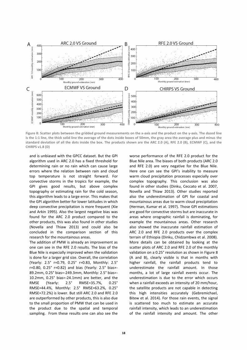
and is unbiased with the GPCC dataset. But the GPI algorithm used in ARC 2.0 has a fixed threshold for determining rain or no rain which can cause large errors where the relation between rain and cloud top temperature is not straight forward. For convective storms in the tropics for example, the GPI gives good results, but above complex topography or estimating rain for the cold season, this algorithm leads to a large error. This makes that the GPI algorithm better for lower latitudes in which deep convective precipitation is more frequent (Xie and Arkin 1995). Also the largest negative bias was found for the ARC 2.0 product compared to the other products, this was also found in other studies (Novella and Thiaw 2013) and could also be concluded in the comparison section of this research for the mountainous areas. The addition of PMW is already an improvement as one can see in the RFE 2.0 results. The bias of the Blue Nile is especially improved when the validation is done for a larger grid size. Overall, the correlation (Yearly: 2.5° r=0.79, 0.25° r=0.83, Monthly: 2.5° r=0.80, 0.25° r=0.82) and bias (Yearly: 2.5° bias=-89.2mm, 0.25° bias=-249.3mm, Monthly: 2.5° bias=-10.2mm, 0.25° bias=-24.1mm) are better, and the RMSE (Yearly: 2.5° RMSE=35.7%, 0.25° RMSE=44.4%, Monthly: 2.5° RMSE=63.2%, 0.25° RMSE=72.2%) is lower. But still ARC 2.0 and RFE 2.0 are outperformed by other products, this is also due to the small proportion of PMW that can be used in the product due to the spatial and temporal sampling. From these results one can also see the

worse performance of the RFE 2.0 product for the Blue Nile area. The biases of both products (ARC 2.0 and RFE 2.0) are very negative for the Blue Nile. Here one can see the GPI’s inability to measure warm cloud precipitation processes especially over complex topography. This conclusion was also found in other studies (Dinku, Ceccato et al. 2007, Novella and Thiaw 2013). Other studies reported also the underestimation of GPI for coastal and mountainous areas due to warm cloud precipitation (Herman, Kumar et al. 1997). Those GPI estimations are good for convective storms but are inaccurate in areas where orographic rainfall is dominating, for example the mountainous areas. Other research also showed the inaccurate rainfall estimation of ARC 2.0 and RFE 2.0 products over the complex terrain of Ethiopia (Dinku, Chidzambwa et al. 2008). More details can be obtained by looking at the scatter plots of ARC 2.0 and RFE 2.0 of the monthly validation on a 0.25° resolution as shown in Figure 8 (A and B), clearly visible is that in months with higher rainfall, the rainfall products tend to underestimate the rainfall amount. In those months, a lot of large rainfall events occur. The underestimation is due to the error which occurs when a rainfall exceeds an intensity of 20 mm/hour, the satellite products are not capable in detecting this high intensities accurately (Gebremichael, Bitew et al. 2014). For those rain events, the signal is scattered too much to estimate an accurate rainfall intensity, which leads to an underestimation of the rainfall intensity and amount. The other

Figure 8: Scatter plots between the gridded ground measurements on the x-axis and the product on the y-axis. The dazed line is the 1:1 line, the thick solid line the average of the dots inside boxes of 50mm, the gray area the average plus and minus the standard deviation of all the dots inside the box. The products shown are the ARC 2.0 (A), RFE 2.0 (B), ECMWF (C), and the CHIRPS v1.8 (D)

19

rainfall products have the same problem, but in a lesser extent.

Instead of the addition of PMW one can also locally calibrate IR signals with ground measurements as done in the TAMSAT algorithm. This improves the measurements a lot as can be seen in the Figure 7. Due to this local calibration the total correlation (Yearly: 2.5° r=0.84, 0.25° r=0.87, Monthly: 2.5° r=0.84, 0.25° r=0.86) and the RMSE (Yearly: 2.5° RMSE =34.8%, 0.25° RMSE =40.9%, Monthly: 2.5° RMSE =56.2%, 0.25° RMSE =60.3%) is improved compared to ARC 2.0 and RFE 2.0. This is a very good result for a product which solely uses IR measurements. The TAMSAT bias for the Blue Nile (Yearly: 2.5° bias=-173.7mm, 0.25° bias=-285.7mm, Monthly: 2.5° bias=-18.2mm, 0.25° bias=-30.8mm) is better than the bias of ARC 2.0 and RFE 2.0 (Yearly: 2.5° bias=-308mm & -233.9mm, 0.25° bias=-420.8mm & -386.1mm, Monthly: 2.5° bias=-30.3mm & -20.9mm, 0.25° bias=-44.6mm & -35.8mm respectively). The local calibration of the IR measurements for the Blue Nile can also be seen in the bias of the Blue Nile, which is on a local 0.25 degree scale much better than ARC 2.0 and RFE 2.0, which use a global IR calibration and therefore based upon 1 fixed threshold for all areas all over the world. ECMWF’s correlations (Yearly: 2.5° r=0.82, 0.25° r=0.82, Monthly: 2.5° r=0.79, 0.25° r=0.82) are more or less the same as RFE 2.0, but the ECMWF’s bias (Yearly: 2.5° bias=-47.2mm, 0.25° bias=-57.9mm, Monthly: 2.5° bias=-5.1mm, 0.25° bias=-4.1mm) is much better. Because the ECMWF rainfall is estimated with the use of a physical based model, it suffers less of the underestimation of rain intensities from the IR measurements, because the empirical relation of cold cloud temperature and rainfall is not used. But the random errors are large and therefore this product is still outperformed by the other products. This is also visible in Figure 8C, which shows a low bias, but a wide uncertainty band. Good to mention is that the ECMWF is outperformed by some products for this certain location. But this product is more accurate at higher latitudes while a satellites product becomes less accurate for higher latitudes due to the placement of the geostationary satellites which are located above the equator. So for higher latitudes ECMWF can be a better product than other satellite products (Xie and Arkin 1996).

GPCP and GPCP1DD show a high correlation (Yearly: 2.5° r=0.88 & 0.85, 0.25° r=0.87 & 0.85, Monthly: 2.5° r=0.88 & 0.87, 0.25° r=0.88 & 0.86 respectively) and also a low RMSE (Yearly: 2.5° RMSE=44.5% & 47.9%, 0.25° RMSE=31.2% & 34.7%, Monthly: 2.5° RMSE=50.3% & 52.4%, 0.25° RMSE= 56.2% & 60.0% respectively). The bias of the GPCP

and GPCP1DD (Yearly: 2.5° bias=-27.8mm & -36.6mm, 0.25° bias=-40.1mm & -92.4mm, Monthly: 2.5° bias=0.9mm & 1.3mm, 0.25° bias=-4.6mm & -9.6mm) are also very low. Those products use the GPI algorithm, but adjust this algorithm by making the rainfall amount variable and the GPCP1DD makes also the rainfall threshold variable. So by adjusting the GPI algorithm the estimation are improved a lot compared to the GPI algorithm used in the ARC 2.0 and RFE 2.0 products. This was also found in a study of Nicholson (Nicholson, Some et al. 2003). The GPCP shows still better results than the GPCP1DD product, but the GPCP1DD is available for daily basis on a 1 degree spatial resolution which can sometimes also be preferred. But still the GPCP1DD has a very coarse resolution compared to other products.

The products that only use ground measurements, CRU TS3.21 and GPCC, also perform very well. A disadvantage is that those products require a denser rain gauge network to obtain a finer spatial resolution which is needed in the future for WA+. Another option is to incorporate remote sensed measurements to interpolate these products into a finer spatial resolution.

When you look at the overall score, the TRMM 3B43 v7 data and CHIRPS v1.8 data have the best performance. In Figure 8D the scatter plot of CHIRPS v1.8 is shown for the monthly 0.25 degrees resolution. The TRMM data has the best bias (Yearly: 2.5° bias=19.7mm, 0.25° bias=-41.9mm, Monthly: 2.5° bias=1.2mm, 0.25° bias =-3mm) of all the products for the Nile basin, and slightly underestimates the rainfall in the mountainous area of the Blue Nile (Yearly: 2.5° bias=-32.6mm, 0.25° bias=-93.1mm, Monthly: 2.5° bias =-3.7mm, 0.25° bias=-9.2mm). But still the RMSE (Yearly: 2.5° RMSE=19.8%, 0.25° RMSE=25.5%, Monthly: 2.5° RMSE=41.4%, 0.25° RMSE=51.1%) and the correlation (Yearly: 2.5° r=0.92, 0.25° r=0.86, Monthly: 2.5° r=0.93, 0.25° r=0.91) are very good for the Blue Nile. The correlations of CHIRPS (Yearly: 2.5° r=0.92, 0.25° r=0.93, Monthly: 2.5° r=0.90, 0.25° r=0.92) are the highest for almost every validated resolution and for a monthly scale the RMSE (Yearly: 2.5° RMSE=25.2%, 0.25° RMSE=28.1%, Monthly: 2.5° RMSE=47.3%, 0.25° RMSE=49.3%) are the lowest. But CHIRPS v1.8 suffers from underestimation of the rainfall as one can see from the bias (Yearly: 2.5° bias=-91mm, 0.25° bias=-138.8mm, Monthly: 2.5° bias =-11mm, 0.25° bias=-14.6mm). For the Blue Nile CHIRPS v1.8 bias has the same underestimation, while for the other products the underestimation becomes more if one compares the bias of the product to the bias of the total Nile Basin, except for TAMSAT and ECMWF. Those good results for CHRIPS v1.8, makes

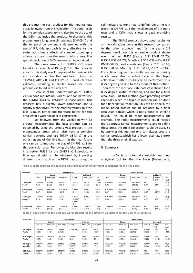
20

this product the best product for the mountainous areas followed from this validation. The good result for the complex topography is also due to the use of the DEM map inside the product. Furthermore, this product use a long term climate map (CHPClim) and the temporal component is determined with the use of IRP, this approach is very effective for the systematic climate effects of complex topography as one can see from the results. Also a very fine spatial resolution of 0.05 degrees can be obtained.

The same results for CHIRPS v1.8 were found in a research of Dinku (2014). The research area for this study was Ethiopia and Tanzania which also includes the Blue Nile sub basin. Here, the TAMSAT, ARC 2.0, and CHIRPS v1.8 products were validated, resulting in similar biases for those products as found in this research.

Because of the underestimation of CHIRPS v1.8 in none mountainous areas, one can better use the TRMM 3B43 v7 datasets in those areas. This datasets has a slightly lower correlation and a slightly higher RMSE for the monthly values, but the bias is much better and therefore better for this area when a water balance is considered.

So, followed from the validation with 62 ground measurements the best product can be obtained by using the CHIRPS v1.8 product in the mountainous areas which also have a complex rainfall patterns and use TRMM 3B43 v7 in the other regions of the Nile Basin. In the near future one can try to improve the bias of CHIRPS v1.8 for this particular area. Removing the bias also results in a better RMSE for the CHIRPS v1.8 product. A finer spatial grid can be obtained by importing different maps, such as the NDVI map or using the

soil moisture content map to define rain or no rain pixels. In CHIRPS v1.8 the involvement of a climate map and a DEM map shows already promising results.

The TRIPLE product shows good results for all the validations done in this research compared to the other products, and for the yearly 2.5 degrees resolution this ensemble product shows even the best RMSE (Yearly: 2.5° RMSE=21.7%, 0.25° RMSE=34.7%, Monthly: 2.5° RMSE=48%, 0.25° RMSE=58.5%) and correlation (Yearly: 2.5° r=0.93, 0.25° r=0.86, Monthly: 2.5° r=0.89, 0.25° r=0.87). For a finer degree the results are less promising which was also expected because the triple collocation method could only be performed on a 0.75 degree grid due to the criteria of this method. Therefore, the most accurate dataset is chosen for a 0.75 degree spatial resolution, and not for a finer resolution. But this method gives promising results especially when the triple collocation can be done for a finer spatial resolution. This can be done if, the model based dataset can be replaced by a finer resolution dataset which is not ground or satellite based. This could be radar measurements for example. The radar measurements could receive more accurate rainfall measurements, and to define those areas the triple collocation could be used. So by applying this method one can always create a rainfall product which has a lower estimated error than the three original datasets. 5. Summary

WA+ is a potentially suitable and new

analytical tool for the Nile Basin (Barendrecht,

Table 5: Table showing the best and worst product for the different validations for the Nile Basin

Nile Basin Best product Worst product

Biased Unbiased Biased Unbiased

Corr (-) RMSE (%) Bias (mm) Corr (-) RMSE (%) Bias (mm)

Corr (-) RMSE (%) Bias (mm) Corr (-) RMSE (%)

Bias (mm)

2.5 Degree Yearly

CMORPH (0.58)

GSMaP (65.9)

GSMaP (188.8)

TRIPLE (0.93)

TRIPLE (21.7)

TRMM (19.7)

PERSIANN (0.26)

PERSIANN (88.9)

CMOPRH (345.9)

ARC (0.71)

ARC (44)

ARC (-144.9)

0.25 Degree Yearly

CMORPH (0.67)

CMORPH (53.2)

PERSIANN (-15.1)

CHIRPS (0.93)

TRMM (26.7)

GPCP (40.1)

PERSIANN (0.17)

PERSIANN (71.4)

CMORPH (175.4)

ECMWF (0.82)

ARC (47.9)

ARC (-287.2)

2.5 Degree Monthly

CMORPH (0.73)

GSMaP (89.2)

GSMaP (15.4)

GPCC/ TRMM/ CHIRPS (0.90)

TRMM (47)

GPCP (0.9)

PERSIANN (0.60)

PERSIANN (117.3)

CMORPH (29.4)

ARC (0.77)

ARC (67)

ARC (-16.3)

0.25 Degree Yearly

CMORPH (0.76)

CMORPH (80.1)

PERSIANN (-0.5)

CHIRPS (0.92)

CHIRPS (49.3)

TRMM (-3.0)

PERSIANN (0.56)

PERSIANN (97.7)

CMORPH (15.8)

ARC (0.81)

RFE (72.2)

ARC (-30.4)

Table 6: Table showing the best and worst product for the different validations for the Blue Nile sub basin

Nile Basin Best product Worst product

Biased Unbiased Biased Unbiased

Corr (-) RMSE (%) Bias (mm) Corr (-) RMSE (%) Bias (mm) Corr (-) RMSE (%) Bias (mm) Corr (-) RMSE (%)

Bias (mm)

2.5 Degree Yearly

CMORPH (0.58)

GSMaP (54.2)

GSMaP (188.8)

CRU (0.96) TRIPLE (19.7)

GPCP (-30.7)

PERSIANN (0.26)

PERSIANN (60.3)

CMORPH (159.3)

ECMWF (0.75)

ARC (47)

ARC (-308)

0.25 Degree Yearly

CMORPH (0.68)

CMORPH (36.6)

CMORPH (19.6)

CHIRPS (0.90)

TRMM (25.5)

ECMWF (79.1)

PERSIANN (0.16)

PERSIANN (56.6)

PERSIANN (-328.1)

ECMWF (0.77)

ARC (46.2)

ARC (-420.8)

2.5 Degree Monthly

CMORPH (0.79)

GSMaP (78.1)

GSMap (-3.7)

CHIRPS/ TRIPLE (0.94)

CHIRPS (40.8)

GPCP (-3.4)

PERSIANN (0.68)

PERSIANN (90.7)

CMORPH (14.6)

ECMWF (0.84)

ARC (67.5)

ARC (-30.3)

0.25 Degree Yearly

CMOPRH (0.82)

CMORPH (68.4)

CMORPH (1.2)

CHIRPS (0.93)

CHIRPS (46.6)

ECMWF (-7.6)

PERSIANN (0.68)

PERSIANN (84.2)

PERSIANN (-34.1)

ARC (0.84)

RFE (74.6)

ARC (-44.6)

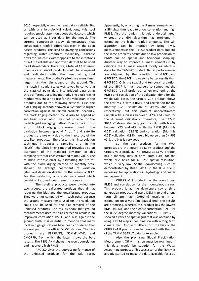
21

2015), especially when the input data is reliable. But as with any hydrological calculations, this tool requires special attention about the datasets which can be used as input data for the model. The current comparison study demonstrates that considerable rainfall differences exist in the open access products. This lead to diverging conclusions regarding water resources availability, utilizable flows etc, which is exactly opposite to the intentions of WA+: a reliable and approved dataset to be used by all stakeholders. Therefore, a total of 13 different open access rainfall products could be compared and validated with the use of ground measurements. The product’s pixels are many times larger than the rain gauges on the ground. This mismatch in spatial scales was solved by converting the classical point data into gridded data using three different upscaling methods. The block kriging method was chosen to use for the validation of the products due to the following reasons. First, the block kriging method showed a systematic higher correlation against all rainfall products. Secondly, the block kriging method could also be applied at sub basin scale, which was not possible for the variable grid averaging method. Due to the intrinsic error in block kriging, the errors found in the validation between ground ”truth” and satellite products are not only due to the inaccuracy of the satellite products. Therefore, this interpolation technique introduces a sampling error in the “truth”. The block kriging method provides also an estimation of the standard deviation of this sampling error for each estimated rainfall value. The founded intrinsic error by estimating the “truth” with the block kriging method on monthly scale showed an average coefficient of variation (standard deviation divided by the mean) of 0.17. For the validation, only grids were used which consist of 1 ground measurements or more.

The satellite products were divided into two groups: the calibrated products that aim at reducing the bias and the uncalibrated products. They were not compared with each other because the ground measurements used for the validation could also be used for the bias removal of the unbiased products. The results show that ground measurements used for bias correction result in an improved correlation RMSE, and bias against the ground truth. It is essential to mention that many local rain gauge stations have been considered that are not part of the official WMO stations. The bias products are PERSIANN, GSMaP_MVK, and CMORPH, from which the latter shows the best results. The PERSIANN shows the worst correlation and has a very high RMSE.

ARC 2.0 gives the poorest performance of the unbiased products for the Nile Basin.

Apparently, by only using the IR measurements with a GPI algorithm leads to a low correlation and high RMSE. Also the rainfall is largely underestimated, whereas the GPI algorithm has problems in estimating the higher rainfall amounts. The GPI algorithm can be improve by using PMW measurements as the RFE 2.0 product does, but still the same problems occurs due to low proportion of PMW due to spatial and temporal sampling. Another way to improve IR measurements is by calibrate the IR measurement locally as which is done for the TAMSAT product. Better performances are obtained by the algorithm of GPCP and GPCP1DD, the GPCP shows some better results than GPCP1DD. Only the spatial and temporal resolution of the GPCP is much coarser, so sometimes the GPCP1DD is still preferred. When one look at the RMSE and correlation of the validation done for the whole Nile basin, the CHIRPS v1.8 product shows the best result with a RMSE and correlation for the monthly 0.25° validation of 49.3% and 0.92 respectively, but this product underestimates rainfall with a biases between -12% and -14% for the different validations. Therefore, the TRMM 3B43 v7 shows also very good results, with biases between +2% and -4%. While the RMSE (Monthly 0.25° validation: 52.3%) and correlation (Monthly 0.25° validation: 0.89%) are a bit worse than CHIRPS v1.8, the bias is very good.

So, the best products for the WA+ purposes are the TRMM 3B43 v7 product and the CHIRPS v1.8 product. The TRMM 3B43 v7 product has a monthly bias of only -3mm (-3%) for the whole Nile basin for a 0.25° spatial resolution, which is very low. Spatial downscaling such as demonstrated by Duan (2014) in the Blue Nile is necessary for applications in hydrology and water management.

CHIRPS v1.8 product has the overall best RMSE and correlation for the mountainous areas. This product is as the developers say a third generation product and use a DEM map and a long term climate map (CPHClim) resulting in an estimation on a very fine spatial grid. The results are promising, whereas this product has the lowest RMSE (46.6%) and the highest correlation (0.93) for the 0.25° degree monthly validations. CHIRPS v1.8 showed a very fine spatial grid that was obtained by using a DEM map in combination with a long term climate map. Also with little effort, the bias of the CHIRPS v1.8 product can be removed with the use of the TRMM 3B43 v7 data for example.

Also the promising Global Precipitation Measurement (GPM) mission must be examined if this data would be superior for the Water Accounting purposes. This successor of the TRMM is already started to make the data available for a 30

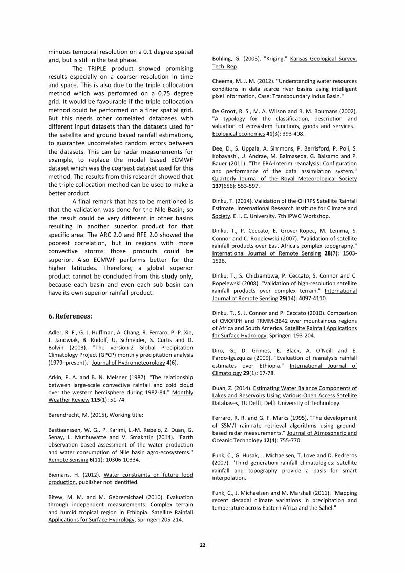
22

minutes temporal resolution on a 0.1 degree spatial grid, but is still in the test phase.

The TRIPLE product showed promising results especially on a coarser resolution in time and space. This is also due to the triple collocation method which was performed on a 0.75 degree grid. It would be favourable if the triple collocation method could be performed on a finer spatial grid. But this needs other correlated databases with different input datasets than the datasets used for the satellite and ground based rainfall estimations, to guarantee uncorrelated random errors between the datasets. This can be radar measurements for example, to replace the model based ECMWF dataset which was the coarsest dataset used for this method. The results from this research showed that the triple collocation method can be used to make a better product

A final remark that has to be mentioned is that the validation was done for the Nile Basin, so the result could be very different in other basins resulting in another superior product for that specific area. The ARC 2.0 and RFE 2.0 showed the poorest correlation, but in regions with more convective storms those products could be superior. Also ECMWF performs better for the higher latitudes. Therefore, a global superior product cannot be concluded from this study only, because each basin and even each sub basin can have its own superior rainfall product.

6. References:

Adler, R. F., G. J. Huffman, A. Chang, R. Ferraro, P.-P. Xie, J. Janowiak, B. Rudolf, U. Schneider, S. Curtis and D. Bolvin (2003). "The version-2 Global Precipitation Climatology Project (GPCP) monthly precipitation analysis (1979–present)." Journal of Hydrometeorology 4(6). Arkin, P. A. and B. N. Meisner (1987). "The relationship between large-scale convective rainfall and cold cloud over the western hemisphere during 1982-84." Monthly Weather Review 115(1): 51-74. Barendrecht, M. (2015), Working title: Bastiaanssen, W. G., P. Karimi, L.-M. Rebelo, Z. Duan, G. Senay, L. Muthuwatte and V. Smakhtin (2014). "Earth observation based assessment of the water production and water consumption of Nile basin agro-ecosystems." Remote Sensing 6(11): 10306-10334. Biemans, H. (2012). Water constraints on future food production, publisher not identified. Bitew, M. M. and M. Gebremichael (2010). Evaluation through independent measurements: Complex terrain and humid tropical region in Ethiopia. Satellite Rainfall Applications for Surface Hydrology, Springer: 205-214.

Bohling, G. (2005). "Kriging." Kansas Geological Survey, Tech. Rep. Cheema, M. J. M. (2012). "Understanding water resources conditions in data scarce river basins using intelligent pixel information, Case: Transboundary Indus Basin." De Groot, R. S., M. A. Wilson and R. M. Boumans (2002). "A typology for the classification, description and valuation of ecosystem functions, goods and services." Ecological economics 41(3): 393-408. Dee, D., S. Uppala, A. Simmons, P. Berrisford, P. Poli, S. Kobayashi, U. Andrae, M. Balmaseda, G. Balsamo and P. Bauer (2011). "The ERA‐Interim reanalysis: Configuration and performance of the data assimilation system." Quarterly Journal of the Royal Meteorological Society 137(656): 553-597. Dinku, T. (2014). Validation of the CHIRPS Satellite Rainfall Estimate. International Research Institute for Climate and Society. E. I. C. University. 7th IPWG Workshop. Dinku, T., P. Ceccato, E. Grover‐Kopec, M. Lemma, S. Connor and C. Ropelewski (2007). "Validation of satellite rainfall products over East Africa's complex topography." International Journal of Remote Sensing 28(7): 1503-1526. Dinku, T., S. Chidzambwa, P. Ceccato, S. Connor and C. Ropelewski (2008). "Validation of high‐resolution satellite rainfall products over complex terrain." International Journal of Remote Sensing 29(14): 4097-4110. Dinku, T., S. J. Connor and P. Ceccato (2010). Comparison of CMORPH and TRMM-3B42 over mountainous regions of Africa and South America. Satellite Rainfall Applications for Surface Hydrology, Springer: 193-204. Diro, G., D. Grimes, E. Black, A. O'Neill and E. Pardo‐Iguzquiza (2009). "Evaluation of reanalysis rainfall estimates over Ethiopia." International Journal of Climatology 29(1): 67-78. Duan, Z. (2014). Estimating Water Balance Components of Lakes and Reservoirs Using Various Open Access Satellite Databases, TU Delft, Delft University of Technology. Ferraro, R. R. and G. F. Marks (1995). "The development of SSM/I rain-rate retrieval algorithms using ground-based radar measurements." Journal of Atmospheric and Oceanic Technology 12(4): 755-770. Funk, C., G. Husak, J. Michaelsen, T. Love and D. Pedreros (2007). "Third generation rainfall climatologies: satellite rainfall and topography provide a basis for smart interpolation." Funk, C., J. Michaelsen and M. Marshall (2011). "Mapping recent decadal climate variations in precipitation and temperature across Eastern Africa and the Sahel."

23

Funk, C., P. Peterson, M. Landsfeld, D. Pedreros, J. Verdin, J. Rowland, B. Romero, G. Husak, J. Michaelsen and A. Verdin (2013). "A Quasi-Global Precipitation Time Series for Drought Monitoring." USGS. Gebremichael, M., M. M. Bitew, F. A. Hirpa and G. N. Tesfay (2014). "Accuracy of satellite rainfall estimates in the Blue Nile Basin: Lowland plain versus highland mountain." Water Resources Research. Grimes, D., E. Pardo-Iguzquiza and R. Bonifacio (1999). "Optimal areal rainfall estimation using raingauges and satellite data." Journal of Hydrology 222(1): 93-108. Grody, N. C. (1991). "Classification of snow cover and precipitation using the Special Sensor Microwave Imager." Journal of Geophysical Research: Atmospheres (1984–2012) 96(D4): 7423-7435. Grossberg, S. (1969). "Embedding fields: A theory of learning with physiological implications." Journal of Mathematical Psychology 6(2): 209-239. Habib, E., M. El Saadani and A. T. Haile (2012). "Climatology-focused evaluation of CMORPH and TMPA satellite rainfall products over the Nile Basin." Journal of Applied Meteorology and Climatology 51(12): 2105-2121. Harris, I., P. Jones, T. Osborn and D. Lister (2013). "Updated high‐resolution grids of monthly climatic observations–the CRU TS3. 10 Dataset." International Journal of Climatology. Herman, A., V. B. Kumar, P. A. Arkin and J. V. Kousky (1997). "Objectively determined 10-day African rainfall estimates created for famine early warning systems." International Journal of Remote Sensing 18(10): 2147-2159. Hsu, K.-l., X. Gao, S. Sorooshian and H. V. Gupta (1997). "Precipitation estimation from remotely sensed information using artificial neural networks." Journal of Applied Meteorology 36(9): 1176-1190. Huffman, G. J., R. F. Adler, P. Arkin, A. Chang, R. Ferraro, A. Gruber, J. Janowiak, A. McNab, B. Rudolf and U. Schneider (1997). "The global precipitation climatology project (GPCP) combined precipitation dataset." Bulletin of the American Meteorological Society 78(1): 5-20. Huffman, G. J., R. F. Adler, D. T. Bolvin, G. Gu, E. J. Nelkin, K. P. Bowman, Y. Hong, E. F. Stocker and D. B. Wolff (2007). "The TRMM Multisatellite Precipitation Analysis (TMPA): Quasi-global, multiyear, combined-sensor precipitation estimates at fine scales." Journal of Hydrometeorology 8(1). Huffman, G. J., R. F. Adler, D. T. Bolvin and E. J. Nelkin (2010). The TRMM multi-satellite precipitation analysis (TMPA). Satellite rainfall applications for surface hydrology, Springer: 3-22.

Huffman, G. J., R. F. Adler, M. M. Morrissey, D. T. Bolvin, S. Curtis, R. Joyce, B. McGavock and J. Susskind (2001). "Global precipitation at one-degree daily resolution from multisatellite observations." Journal of Hydrometeorology 2(1): 36-50. Huffman, G. J. and D. T. Bolvin (2007). "TRMM and other data precipitation data set documentation." Laboratory for Atmospheres, NASA Goddard Space Flight Center and Science Systems and Applications. Islam, T., P. K. Srivastava, M. A. Rico-Ramirez, Q. Dai, D. Han and M. Gupta (2014). "An exploratory investigation of an adaptive neuro fuzzy inference system (ANFIS) for estimating hydrometeors from TRMM/TMI in synergy with TRMM/PR." Atmospheric Research 145: 57-68. Janssen, P. A., S. Abdalla, H. Hersbach and J.-R. Bidlot (2007). "Error estimation of buoy, satellite, and model wave height data." Journal of Atmospheric and Oceanic Technology 24(9): 1665-1677. Joyce, R. J., J. E. Janowiak, P. A. Arkin and P. Xie (2004). "CMORPH: A method that produces global precipitation estimates from passive microwave and infrared data at high spatial and temporal resolution." Journal of Hydrometeorology 5(3). Joyce, R. J., P. Xie, Y. Yarosh, J. E. Janowiak and P. A. Arkin (2010). CMORPH: A “Morphing” Approach for High Resolution Precipitation Product Generation. Satellite Rainfall Applications for Surface Hydrology, Springer: 23-37. Karimi, P., W. Bastiaanssen and D. Molden (2013). "Water Accounting Plus (WA+)–a water accounting procedure for complex river basins based on satellite measurements." Hydrology and Earth System Sciences 17(7): 2459-2472. Karimi, P., W. Bastiaanssen, A. Sood, J. Hoogeveen, L. Peiser, E. Bastidas-Obando and R. Dost (2014). "Spatial evapotranspiration, rainfall and land use data in water accounting–Part 2: Reliability of water accounting results for policy decisions in the Awash basin." Hydrology and Earth System Sciences Discussions 11(1): 1125-1167. Karimi, P., D. Molden, W. Bastiaanssen and X. Cai (2012). "4. Water accounting to assess use and productivity of water: evolution of a concept and new frontiers." Water Accounting: International Approaches to Policy and Decision-making: 76. Kawanishi, T., H. Kuroiwa, M. Kojima, K. Oikawa, T. Kozu, H. Kumagai, K. i. Okamoto, M. Okumura, H. Nakatsuka and K. Nishikawa (2000). "TRMM precipitation radar." Advances in Space Research 25(5): 969-972. Kidd, C., V. Levizzani, J. Turk and R. Ferraro (2009). "Satellite Precipitation Measurements for Water Resource Monitoring1." JAWRA Journal of the American Water Resources Association 45(3): 567-579.

24

Kohonen, T. (1982). "Self-organized formation of topologically correct feature maps." Biological cybernetics 43(1): 59-69. Kozu, T., T. Kawanishi, H. Kuroiwa, M. Kojima, K. Oikawa, H. Kumagai, K. i. Okamoto, M. Okumura, H. Nakatsuka and K. Nishikawa (2001). "Development of precipitation radar onboard the Tropical Rainfall Measuring Mission (TRMM) satellite." Geoscience and Remote Sensing, IEEE Transactions on 39(1): 102-116. Kubota, T., S. Shige, H. Hashizume, K. Aonashi, N. Takahashi, S. Seto, Y. N. Takayabu, T. Ushio, K. Nakagawa and K. Iwanami (2007). "Global precipitation map using satellite-borne microwave radiometers by the GSMaP Project: Production and validation." Geoscience and Remote Sensing, IEEE Transactions on 45(7): 2259-2275. Kummerow, C. and L. Giglio (1995). "A method for combining passive microwave and infrared rainfall observations." Journal of Atmospheric and Oceanic Technology 12(1): 33-45. Kurukulasuriya, P. and S. Rosenthal (2013). "Climate change and agriculture: a review of impacts and adaptations." Liu, G. and J. A. Curry (1992). "Retrieval of precipitation from satellite microwave measurement using both emission and scattering." Journal of Geophysical Research: Atmospheres (1984–2012) 97(D9): 9959-9974. Love, T. B., V. Kumar, P. Zie and W. Thiaw (2004). "A 20-Year Daily Africa Precipitation Climatology Using Satellite and Gauge Data." 14th Conf. on Applied Meteorology. Mandel, J. (1964). "The statistical analysis of experimental data." Mineola, NY: Dover Publications 410. Marsden, R. F. (1999). "A proposal for a neutral regression." Journal of Atmospheric and Oceanic Technology 16(7): 876-883. Mitchell, T. D. and P. D. Jones (2005). "An improved method of constructing a database of monthly climate observations and associated high‐resolution grids." International journal of climatology 25(6): 693-712. Molden, D. (1997). Accounting for water use and productivity, Iwmi. Narjary, B. and S. Kamra (2013). "Impact of climatic variability on groundwater resources in fresh ground water region of Haryana." Climate Change Impact on Salt-affected Soils and Their Crop Productivity: 51. Nicholson, S. E., B. Some, J. McCollum, E. Nelkin, D. Klotter, Y. Berte, B. Diallo, I. Gaye, G. Kpabeba and O. Ndiaye (2003). "Validation of TRMM and other rainfall estimates with a high-density gauge dataset for West Africa. Part I: Validation of GPCC rainfall product and pre-TRMM satellite and blended products." Journal of Applied Meteorology 42(10): 1337-1354.

Nicholson, S. E., B. Some, J. McCollum, E. Nelkin, D. Klotter, Y. Berte, B. Diallo, I. Gaye, G. Kpabeba and O. Ndiaye (2003). "Validation of TRMM and other rainfall estimates with a high-density gauge dataset for West Africa. Part II: Validation of TRMM rainfall products." Journal of Applied Meteorology 42(10): 1355-1368. NOAA (2001). "The NOAA Climate Prediction Center African Rainfall Estimation Algorithm Version 2.0." Novella, N. S. and W. M. Thiaw (2013). "African Rainfall Climatology Version 2 for Famine Early Warning Systems." Journal of Applied Meteorology & Climatology 52(3). Oki, T. and S. Kanae (2006). "Global hydrological cycles and world water resources." science 313(5790): 1068-1072. OSCAR. (2014). "List of all Satellites." Retrieved 11 May, 2014, from http://www.wmo-sat.info/oscar/satellites. Rijsberman, F. R. (2006). "Water scarcity: fact or fiction?" Agricultural water management 80(1): 5-22. Roebeling, R., E. Wolters, J. Meirink and H. Leijnse (2012). "Triple collocation of summer precipitation retrievals from SEVIRI over Europe with gridded rain gauge and weather radar data." Journal of Hydrometeorology 13(5): 1552-1566. Romilly, T. and M. Gebremichael (2011). "Evaluation of satellite rainfall estimates over Ethiopian river basins." Hydrology and Earth System Sciences 15(5): 1505-1514. Russchenberg, H. and L. P. Ligthart (1996). "Backscattering by and propagation through the melting layer of precipitation: A new polarimetric model." Geoscience and Remote Sensing, IEEE Transactions on 34(1): 3-14. Seckler, D. W. (1998). World water demand and supply, 1990 to 2025: Scenarios and issues, Iwmi. Serrat‐Capdevila, A., J. B. Valdes and E. Z. Stakhiv (2013). "Water Management Applications for Satellite Precipitation Products: Synthesis and Recommendations." JAWRA Journal of the American Water Resources Association. Shepard, D. (1968). A two-dimensional interpolation function for irregularly-spaced data. Proceedings of the 1968 23rd ACM national conference, ACM. Sorooshian, S., K.-L. Hsu, X. Gao, H. V. Gupta, B. Imam and D. Braithwaite (2000). "Evaluation of PERSIANN system satellite-based estimates of tropical rainfall." Bulletin of the American Meteorological Society 81(9): 2035-2046. Stoffelen, A. (1998). "Toward the true near‐surface wind speed: Error modeling and calibration using triple collocation." Journal of Geophysical Research: Oceans (1978–2012) 103(C4): 7755-7766. Sutherland, W. J., R. P. Freckleton, H. C. J. Godfray, S. R. Beissinger, T. Benton, D. D. Cameron, Y. Carmel, D. A.

25

Coomes, T. Coulson and M. C. Emmerson (2013). "Identification of 100 fundamental ecological questions." Journal of ecology 101(1): 58-67. Thépaut, J. N., P. Courtier, G. Belaud and G. Lemaǐtre (1996). "Dynamical structure functions in a four‐dimensional variational assimilation: A case study." Quarterly Journal of the Royal Meteorological Society 122(530): 535-561. Thiemig, V., R. Rojas, M. Zambrano-Bigiarini, V. Levizzani and A. De Roo (2012). "Validation of satellite-based precipitation products over sparsely gauged African river basins." Journal of Hydrometeorology 13(6): 1760-1783. Thorne, V., P. Coakeley, D. Grimes and G. Dugdale (2001). "Comparison of TAMSAT and CPC rainfall estimates with raingauges, for southern Africa." International Journal of Remote Sensing 22(10): 1951-1974. Ushio, T. and M. Kachi (2010). Kalman filtering applications for global satellite mapping of precipitation (GSMaP). Satellite Rainfall Applications for Surface Hydrology, Springer: 105-123. Ushio, T., K. Sasashige, T. Kubota, S. Shige, K. i. Okamoto, K. Aonashi, T. Inoue, N. Takahashi, T. Iguchi and M. Kachi (2009). "A Kalman filter approach to the Global Satellite Mapping of Precipitation (GSMaP) from combined passive microwave and infrared radiometric data." Journal of the Meteorological Society of Japan 87: 137-151. Vogelzang, J. and A. Stoffelen (2012). "Triple collocation."

Vrugt, J. A., C. G. Diks, H. V. Gupta, W. Bouten and J. M. Verstraten (2005). "Improved treatment of uncertainty in hydrologic modeling: Combining the strengths of global optimization and data assimilation." Water Resources Research 41(1). Wilheit, T. T. (1986). "Some comments on passive microwave measurement of rain." Bulletin of the American Meteorological Society 67(10): 1226-1232. Wilheit, T. T., A. T. Chang and L. S. Chiu (1991). "Retrieval of monthly rainfall indices from microwave radiometric measurements using probability distribution functions." Journal of Atmospheric and Oceanic Technology 8(1): 118-136. Willmott, C. J., S. M. Robeson and J. J. Feddema (1994). "Estimating continental and terrestrial precipitation averages from rain‐gauge networks." International Journal of Climatology 14(4): 403-414. Xie, P. and P. A. Arkin (1995). "An intercomparison of gauge observations and satellite estimates of monthly precipitation." Journal of Applied Meteorology 34(5): 1143-1160. Xie, P. and P. A. Arkin (1996). "Analyses of global monthly precipitation using gauge observations, satellite estimates, and numerical model predictions." Journal of climate 9(4): 840-858.

26

Appendix A: List of Abbreviations 4D-VAR = Four Dimensional Variation Assimilation System AGPI = Adjusted GOES Precipitation Index AMSU = Advanced Microwave Sounding Unit AMSR = Advanced Microwave Scanning Radiometer ARC = Africa Rainfall Climatology CAM = Climate Anomaly Method CCD = Cold Cloud Duration CHG = Climate Hazards Group CLIMAT = Names of the codes for reporting monthly values of meteorological parameters CMORPH = Climate Prediction Center Morphing Method CHIRP = Climate Hazards Group IR Precipitation CHIRPS = Climate Hazards Group IR Precipitation Station CHPClim = CHG Precipitation Climatology CPC = Climate Prediction Center CRU_TS = Climatic Research Unit Time Series CSAV = Cloud System Advection Vector map DEM = Digital Elevation Model DWD = Deutcher Wetterdienst ECMWF = European Centre for Medium-Range Weather Forecasts ERA-interim = ECMWF Interim Reanalysis FAO = Food and Agriculture Organization of the United Nations FEWS NET = Famine Early Warning System Network GANAL = JMA Global Analysis GEO = Geostationary Orbit GHCN = Global Historical Climatology Network GOES = Geostationary Operational Environmental Satellite GPCC = Global Precipitation Climatology Centre GPCP = Global Precipitation Climatology Project GPCP1DD = Global Precipitation Climatology Project 1 Degree Daily GPI = GOES Precipitation Index GPROF = Goddard Profiling Algorithm GPM = Global Precipitation Measurement GSMaP = Global Satellite Mapping of Precipitation GSMap_MVK = Global Satellite Mapping of Precipitation Moving Vector with Kalman version GTS = Global Telecommunication system HYDRO1K = Geographic database developed of topographically derived data sets IFS = Integrated Forecast System IR = Infra Red IRP = IR Precipitation JAXA = Japan Aerospace Exploration Agency JMA = Japan Meteorological Agency LEO = Low Earth Orbit PERSIANN = Precipitation Estimation from Remotely Sensed Information Using Artificial Neural Networks PR = Precipitation Radar MCDW = Monthly Climatic Data for the World MGLL = Modified Grossberg Linear Layer NASA = National Aeronautics and Space Administration NBI = Nile Basin Initiative NESDIS = National Environmental Satellite Data and Information Service NDVI = Normalized Difference Vegetation Index NOAA = National Oceanic and Atmospheric Administration RFE = African Rainfall Estimation Algorithm RMSE = Root Mean Squared Error RNC = Rain/No Rain Classification SEVIRI = Spinning Enhanced Visible Infra-Red Imager SOFM = Self Organizing Feature Map SPHEREMAP = Shephards Method in Spherical Coordinates SSM/I = Special Sensor Microwave-Imager TAMSAT = Tropical Applications of Meteorology using Satellite data and Ground-Based Observations TIR = Thermal Infrared TMI = TRMM Microwave Imager TMPA = TRMM Multi-satellite Precipitation Analysis TMPI = Threshold-Matched Precipitation Index TRMM = Tropical Rainfall Measuring Mission USGS = United States Geological Survey’s VAR = Variable Rain rate VIS = Visible light WA+ = Water Accounting Plus WCRP = World Climate Research Programme WWR = World Weather Records

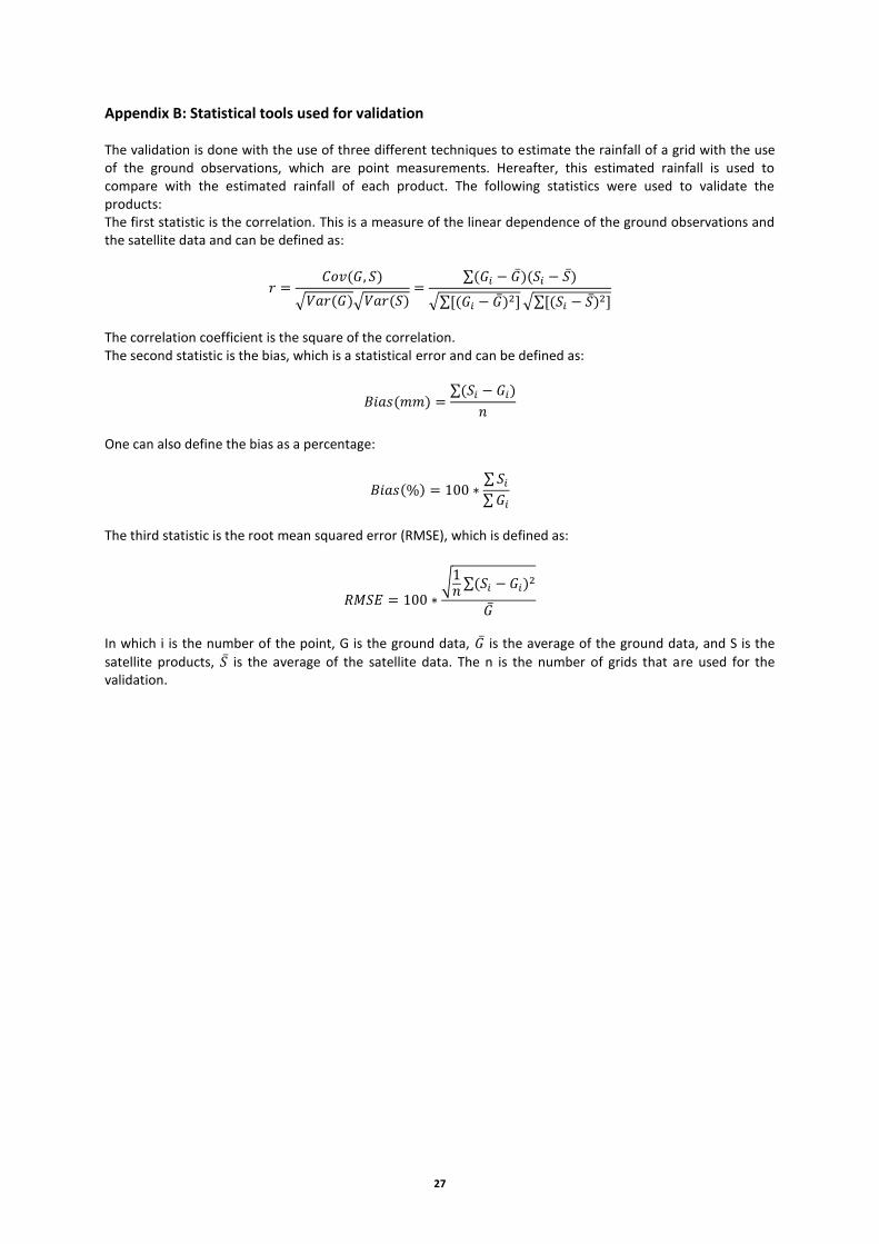
27

Appendix B: Statistical tools used for validation

The validation is done with the use of three different techniques to estimate the rainfall of a grid with the use of the ground observations, which are point measurements. Hereafter, this estimated rainfall is used to compare with the estimated rainfall of each product. The following statistics were used to validate the products: The first statistic is the correlation. This is a measure of the linear dependence of the ground observations and the satellite data and can be defined as:

The correlation coefficient is the square of the correlation. The second statistic is the bias, which is a statistical error and can be defined as:

One can also define the bias as a percentage:

The third statistic is the root mean squared error (RMSE), which is defined as:

In which i is the number of the point, G is the ground data, is the average of the ground data, and S is the

satellite products, is the average of the satellite data. The n is the number of grids that are used for the validation.

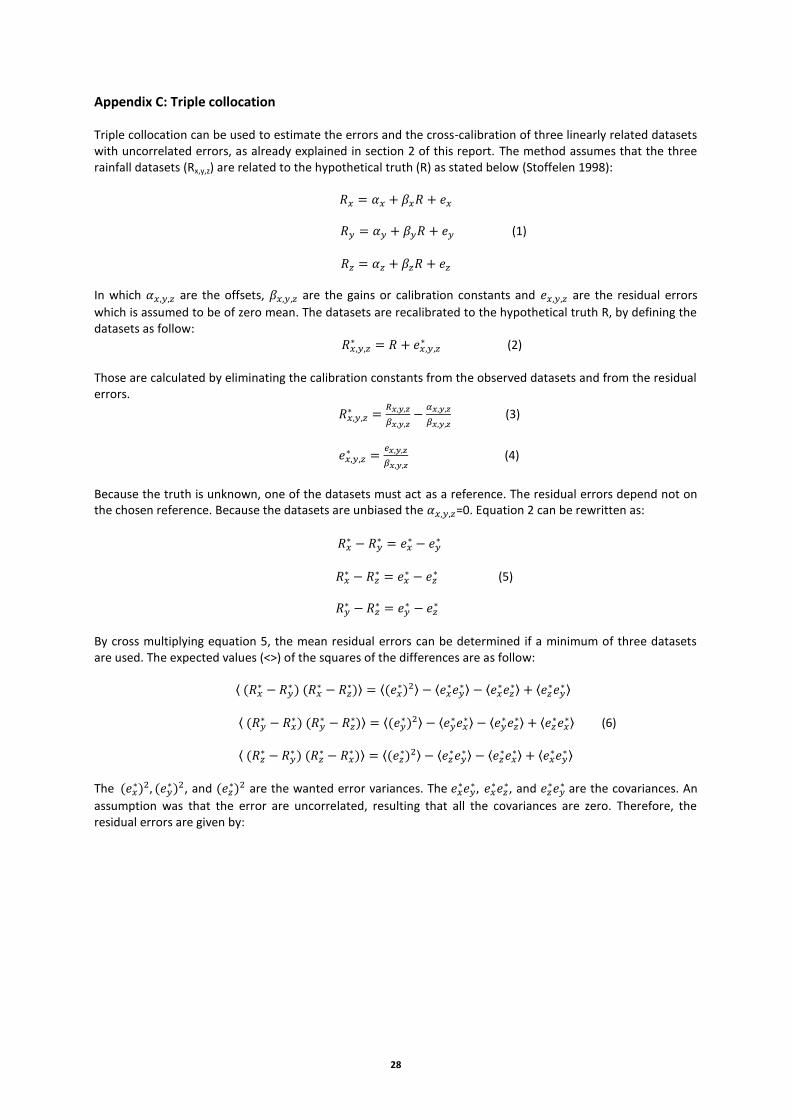
28

Appendix C: Triple collocation

Triple collocation can be used to estimate the errors and the cross-calibration of three linearly related datasets with uncorrelated errors, as already explained in section 2 of this report. The method assumes that the three rainfall datasets (Rx,y,z) are related to the hypothetical truth (R) as stated below (Stoffelen 1998):

(1)

In which are the offsets, are the gains or calibration constants and are the residual errors

which is assumed to be of zero mean. The datasets are recalibrated to the hypothetical truth R, by defining the datasets as follow:

(2)

Those are calculated by eliminating the calibration constants from the observed datasets and from the residual errors.

(3)

(4)

Because the truth is unknown, one of the datasets must act as a reference. The residual errors depend not on the chosen reference. Because the datasets are unbiased the =0. Equation 2 can be rewritten as:

(5)

By cross multiplying equation 5, the mean residual errors can be determined if a minimum of three datasets are used. The expected values (<>) of the squares of the differences are as follow:

(6)

The

, and are the wanted error variances. The

, and

are the covariances. An

assumption was that the error are uncorrelated, resulting that all the covariances are zero. Therefore, the residual errors are given by:

29

6)

By assuming that dataset x is calibrated , the other two systems can be calibrated by using x as reference. So by using the neutral regression one can find and . The equations used in the neutral

regression (Marsden 1999) are stated below to calculate the calibration constant (Janssen, Abdalla et al. 2007):

(7)

Where;

(8)

(9)

(10)

(11)

The can be found by replacing y with z in equation 8 till 11. After those calculations all the calibration constants are known and one can repeat the whole calculation again but now by using the calibration constant of equations 3 to adjust the observed rainfall. Repeat those steps until convergence is obtained, so when all the calibration constants become 1. With the error, the standard deviation can be calculated by the following relationship between error and standard deviation:

For this report the means of the errors are taken for every grid for a period of time. A large time period is needed to guarantee that the mean errors are Gaussian, which is one of the main criteria for the triple collocation method. The above calculations are done in Matlab with 1000 iteration steps to ensure convergence. The results of this calculation are shown in the next section. Those calculations are done for two periods, namely the wet and the dry period of the Nile basin. The periods are both 6 months and are from May till October (wet period) and from November till April (dry period). Periods with fewer months were not possible, to ensure a Gaussian distribution of the errors.

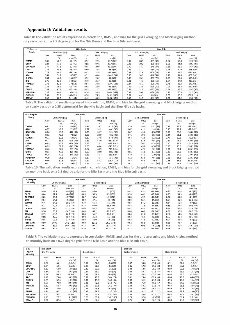
30

Appendix D: Validation results

Table 7: The validation results expressed in correlation, RMSE, and bias for the grid averaging and block kriging method on monthly basis on a 0.25 degree grid for the Nile Basin and the Blue Nile sub basin.

0.25 Degree Monthly

Nile Basin Blue Nile

Grid Averaging Block Kriging Grid Averaging Block Kriging

Corr -

RMSE %

Bias mm (%)

Corr -

RMSE %

Bias mm (%)

Corr -

RMSE %

Bias mm (%)

Corr -

RMSE %

Bias mm (%)

TRMM 0.86 55.1 -6.6 (94) 0.89 52.3 -3.0 (97) 0.87 54.8 -15.2 (89) 0.91 51.1 -9.2 (92) GPCP 0.84 59.1 -8.6 (93) 0.88 56.2 -4.6 (95) 0.86 57.8 -15.7 (88) 0.90 53.8 -9.4 (92) GPCP1DD 0.82 63.0 -14.0 (88) 0.86 60.0 -9.6 (91) 0.84 62.6 -25.2 (82) 0.89 59.1 -17.8 (84) CRU 0.84 58.5 -10.3 (91) 0.87 55.0 -6.6 (94) 0.84 59.1 -17.3 (87) 0.88 55.1 -11.3 (91) ECMWF 0.78 69.5 -8.2 (93) 0.82 68.9 -4.4 (96) 0.82 63.5 -13.5 (90) 0.86 62.0 -7.6 (94) ARC 0.78 73.4 -35.5 (71) 0.81 70.9 -30.4 (73) 0.81 73.4 -52.4 (64) 0.84 70.6 -44.6 (66) CHIRPS 0.89 52.6 -19.3 (84) 0.92 49.3 -14.6 (86) 0.90 51.2 -23.1 (83) 0.93 46.6 -16.4 (85) RFE 0.79 73.0 -29.7 (74) 0.82 72.2 -24.1 (76) 0.82 75.0 -45.0 (67) 0.85 74.6 -35.8 (69) TAMSAT 0.82 64.7 -30.5 (76) 0.86 60.3 -26.1 (77) 0.84 63.2 -37.6 (74) 0.88 58.2 -30.8 (76) GPCC 0.85 55.0 -11.8 (90) 0.89 49.8 -8.2 (93) 0.84 56.9 -19.1 (87) 0.89 50.8 -13.5 (89) TRIPLE 0.84 61.7 -18.2 (85) 0.87 58.5 -13.5 (87) 0.86 61.7 -31.0 (77) 0.90 57.5 -23.0 (80)

PERSIANN 0.51 97.1 -3.5 (97) 0.56 97.7 -0.5 (100) 0.63 85.4 -41.7 (71) 0.68 84.2 -34.1 (73) CMORPH 0.73 77.7 14.1 (112) 0.76 80.1 15.8 (115) 0.79 67.0 -3.9 (97) 0.82 68.4 1.2 (101) GSMaP 0.66 82.4 -9.8 (91) 0.70 82.5 -6.3 (94) 0.76 74.9 -36.8 (74) 0.80 73.8 -28.9 (76)

Table 8: The validation results expressed in correlation, RMSE, and bias for the grid averaging and block kriging method on yearly basis on a 2.5 degree grid for the Nile Basin and the Blue Nile sub basin.

2.5 Degree Yearly

Nile Basin Blue Nile

Grid Averaging Block Kriging Grid Averaging Block Kriging

Corr -

RMSE %

Bias mm (%)

Corr -

RMSE %

Bias mm (%)

Corr -

RMSE %

Bias mm (%)

Corr -

RMSE %

Bias mm (%)

TRMM 0.85 40.9 -27 (97) 0.92 22.5 19.7 (102) 0.92 28.9 -139 (87) 0.92 19.8 -32.6 (96) GPCP 0.82 44.5 -33 (96) 0.88 27.6 28.7 (104) 0.92 30.2 -136 (87) 0.88 24.0 -30.7 (97) GPCP1DD 0.79 47.6 -32 (96) 0.85 29.9 36.6 (105) 0.90 33.7 -145 (87) 0.86 26.1 -36.4 (96) CRU 0.82 45.6 -79 (90) 0.90 24.5 -33.6 (96) 0.89 37.2 -230 (79) 0.96 20.0 -128.6 (86) ECMWF 0.78 49.7 -89 (89) 0.82 37.4 -47.2 (94) 0.83 37.6 -200 (81) 0.75 39.7 -121.7 (87) ARC 0.69 59.7 -187 (77) 0.71 44.0 -144.9 (81) 0.86 54.7 -418 (61) 0.76 47.0 -308.0 (67) CHIRPS 0.84 46.8 -154 (81) 0.92 25.2 -91.0 (88) 0.96 35.1 -257 (76) 0.93 25.4 -155.5 (83) RFE 0.76 52.9 -142 (83) 0.79 35.7 -89.2 (88) 0.91 44.7 -338 (68) 0.84 37.9 -233.9 (74) TAMSAT 0.78 52.8 -172 (79) 0.84 34.8 -130.7 (83) 0.84 45.1 -278 (74) 0.78 36.4 -173.7 (81) GPCC 0.88 36.9 -91 (89) 0.92 22.9 -43.2 (94) 0.92 32.9 -215 (80) 0.93 22.3 -112.3 (88) TRIPLE 0.84 43.6 -90 (89) 0.93 21.7 -39.9 (95) 0.94 31.0 -197 (83) 0.94 19.7 -95.5 (90)

PERSIANN 0.36 90.1 194 (124) 0.26 88.9 300.8 (139) 0.32 59.8 -176 (84) 0.16 60.3 -51.3 (94) CMORPH 0.59 73.8 208 (125) 0.58 76.5 345.9 (146) 0.69 43.1 51 (105) 0.50 56.7 159.3 (118) GSMaP 0.52 68.5 94 (111) 0.42 65.9 188.8 (124) 0.50 51.5 -141 (87) 0.30 54.2 -25.2 (97)

Table 9: The validation results expressed in correlation, RMSE, and bias for the grid averaging and block kriging method on yearly basis on a 0.25 degree grid for the Nile Basin and the Blue Nile sub basin.

0.25 Degree Yearly

Nile Basin Blue Nile

Grid Averaging Block Kriging Grid Averaging Block Kriging

Corr -

RMSE %

Bias mm (%)

Corr -

RMSE %

Bias mm (%)

Corr -

RMSE %

Bias mm (%)

Corr -

RMSE %

Bias mm (%)

TRMM 0.81 43.1 -48 (95) 0.91 26.7 -41.9 (96) 0.70 39.3 -131 (89) 0.86 25.5 -93.1 (92) GPCP 0.77 47.3 -72 (93) 0.87 31.2 -40.1 (96) 0.67 41.1 -141(89) 0.80 29.7 -92.2 (92) GPCP1DD 0.76 49.0 -122 (88) 0.85 34.7 -92.4 (90) 0.67 43.6 -230 (82) 0.80 33.0 -188.6 (84) CRU 0.82 42.8 -78 (92) 0.90 28.0 -72.2 (92) 0.71 39.1 -153 (88) 0.84 28.1 -132.6 (89) ECMWF 0.71 53.3 -63 (94) 0.82 37.8 -57.9 (94) 0.64 42.8 -122 (90) 0.77 32.3 -79.1 (93) ARC 0.77 55.5 -278 (72) 0.83 47.9 -287.2 (70) 0.71 52.6 -454 (64) 0.81 46.2 -420.8 (65) CHIRPS 0.85 43.3 -174 (82) 0.93 28.1 -138.8 (85) 0.81 36.7 -218 (83) 0.90 26.4 -181.0 (85) RFE 0.79 52.2 -247 (74) 0.83 44.4 -249.3 (73) 0.73 49.8 -418 (67) 0.80 43.8 -386.1 (67) TAMSAT 0.76 52.7 -233 (76) 0.87 40.9 -226.9 (76) 0.71 47.7 -321 (74) 0.82 38.4 -285.7 (76) GPCC 0.81 43.6 -101 (90) 0.89 30.0 -88.2 (91) 0.66 41.8 -174 (86) 0.80 30.2 -133.7 (89) TRIPLE 0.78 47.2 -140 (86) 0.86 34.7 -136.3 (86) 0.70 44.1 -279 (78) 0.83 34.2 -249.4 (79)

PERSIANN 0.29 76.6 -51 (94) 0.17 71.4 -15.1 (98) 0.12 63.8 -404 (68) 0.16 56.6 -328.1 (72) CMORPH 0.66 57.5 81 (108) 0.67 53.2 175.4 (119) 0.57 44.8 -45 (97) 0.68 36.6 19.6 (102) GSMaP 0.51 61.8 -89 (91) 0.43 57.2 -66.3 (93) 0.42 52.7 -332 (73) 0.45 48.7 -294.7 (75)

Table 10: The validation results expressed in correlation, RMSE, and bias for the grid averaging and block kriging method on monthly basis on a 2.5 degree grid for the Nile Basin and the Blue Nile sub basin.

2.5 Degree Monthly

Nile Basin Blue Nile

Grid Averaging Block Kriging Grid Averaging Block Kriging

Corr -

RMSE %

Bias mm (%)

Corr -

RMSE %

Bias mm (%)

Corr -

RMSE %

Bias mm (%)

Corr -

RMSE %

Bias mm (%)

TRMM 0.86 49.9 -2.6 (97) 0.90 47.0 1.2 (101) 0.91 45.1 -14.1 (88) 0.93 41.4 -3.7 (95) GPCP 0.84 52.4 -3.0 (97) 0.88 50.3 0.9 (101) 0.90 46.1 -13.9 (88) 0.93 43.3 -3.4 (96) GPCP1DD 0.82 55.8 -2.7 (97) 0.87 52.4 1.3 (102) 0.88 49.9 -14.9 (87) 0.92 45.0 -4.1 (95) CRU 0.84 54.0 -9.4 (90) 0.89 47.1 -4.6 (94) 0.89 52.4 -24.0 (79) 0.94 41.3 -12.0 (86) ECMWF 0.76 64.6 -10.9 (89) 0.79 65.4 -5.1 (94) 0.85 57.2 -22.0 (81) 0.84 61.3 -9.9 (89) ARC 0.73 70.9 -23.1 (77) 0.77 67.0 -16.3 (80) 0.84 71.9 -44.3 (61) 0.85 67.5 -30.3 (67) CHIRPS 0.86 53.0 -17.0 (83) 0.90 47.3 -11 (86) 0.92 48.5 -26.1 (77) 0.94 40.8 -13.8 (84) RFE 0.76 66.5 -16.5 (83) 0.80 63.2 -10.2 (87) 0.86 66.2 -34.2 (69) 0.87 62.8 -20.9 (76) TAMSAT 0.79 63.7 -22.1 (78) 0.84 56.2 -16.1 (81) 0.84 61.8 -30.4 (73) 0.88 54.6 -18.2 (80) GPCC 0.88 47.6 -10.4 (90) 0.90 45.3 -5.3 (93) 0.92 46.9 -22.3 (80) 0.93 41.4 -10.7 (88) TRIPLE 0.85 53.9 -11.4 (88) 0.89 48.0 -5.6 (93) 0.92 47.6 -20.4 (82) 0.94 39.4 -8.4 (90)

PERSIANN 0.50 109.3 26.1 (126) 0.60 117.3 26.2 (132) 0.62 85.9 -17.3 (85) 0.68 90.7 -6.6 (93) CMORPH 0.67 89.1 30.4 (131) 0.73 97.7 29.4 (137) 0.78 69.5 8.6 (108) 0.79 81.4 14.6 (117) GSMaP 0.63 84.1 14.0 (114) 0.70 89.2 15.4 (119) 0.72 73.5 -14.2 (88) 0.76 78.1 -3.7 (96)

31

Table 11: The validation result expressed in correlation, RMSE, and bias for the variable grid averaging method on a monthly and a yearly basis.

Variable Grid Averaging Yearly Monthly

Corr -

RMSE %

Bias mm (%)

Correlation -

RMSE %

Bias mm (%)

TRMM 0.88 28.6 -141.66 (87) 0.95 39.9 -12.26 (88) GPCP 0.88 30.2 -150.71 (86) 0.94 42.4 -12.86 (87) GPCP1DD 0.89 29.6 -142.13 (87) 0.94 43.2 -12.11 (88) CRU 0.84 36.5 -238.59 (77) 0.91 52.5 -22.32 (78) ECMWF 0.81 36.6 -201.27 (81) 0.88 57.1 -18.19 (82) ARC 0.86 48.7 -388.98 (63) 0.90 69.0 -38.42 (64) CHIRPS 0.91 34.9 -266.27 (75) 0.96 45.0 -24.24 (76) RFE 0.87 44.9 -341.45 (67) 0.90 67.3 -32.38 (68) TAMSAT 0.87 40.1 -288.93 (72) 0.92 55.0 -28.54 (73) GPCC 0.88 31.9 -210.61 (80) 0.94 43.7 -19.2 (82) TRIPLE 0.91 39.0 -294.40 (72) 0.95 52.4 -27.4 (73)

PERSIANN 0.37 50.9 -52.55 (95) 0.74 77.9 -2.17 (98) CMORPH 0.76 37.8 118.04 (111) 0.87 61.3 15.8 (116) GSMaP 0.58 42.6 -66.77 (94) 0.82 63.6 -6.35 (94)

32

Basic Principles of Satellite Precipitation Measurements Introduction of open access precipitation products

TU Delft Tim M. Hessels Prof. Dr. Wim G. M. Bastiaanssen

Basic Principles of Satellite Precipitation Measurements

1

Basic Principles of Satellite Precipitation Measurements

2

Table of Contents 1. Introduction ......................................................................................................................................... 4

2. Satellites missions ............................................................................................................................... 4

2.1 Operational Geostationary satellites ............................................................................................ 4

2.2 Operational Low orbiting satellites ............................................................................................... 5

3. Basic techniques .................................................................................................................................. 8

3.1 Geostationary satellites ................................................................................................................. 8

3.1.1 Passive microwave techniques ............................................................................................... 8

3.2 Low orbiting satellites ................................................................................................................... 9

3.2.1 Passive microwave ................................................................................................................. 9

3.2.2 Active microwave ................................................................................................................. 10

4. Rainfall product algorithms ............................................................................................................... 12

4.1 TRMM 3B43 ................................................................................................................................. 12

4.1.1 Retrieval Algorithm for TMI, AMSR-E and SSM-I sensors..................................................... 13

4.1.2 Retrieval Algorithm for AMSU-B and MHS sensors .............................................................. 14

4.1.3 Retrieval Algorithm for the IR data ...................................................................................... 14

4.1.4 Combining products with TMPA ........................................................................................... 14

4.2 CMORPH ...................................................................................................................................... 18

4.2.1 Retrieval Algorithm for SSM-I/SSMIS sensor ........................................................................ 18

4.2.2 Normalization of the microwave derived precipitation estimates ...................................... 18

4.2.3 Combining satellite products with the morphing technique ............................................... 19

4.3 GPCP V2.2 .................................................................................................................................... 21

4.3.1 Retrieval Algorithm for the SSM-I/SSMIS and AIRS .............................................................. 21

4.3.2 Retrieval Algorithm for the IR estimates .............................................................................. 23

4.3.3 Obtaining the AGPI from the GPI ......................................................................................... 23

4.3.4 Combining satellite products to obtain GPCP ...................................................................... 23

4.4 GPCP 1DD .................................................................................................................................... 25

4.4.1 Obtaining the TMPI from the GPI ......................................................................................... 25

4.4.2 Retrieval algorithm for the TOVS and AIRS .......................................................................... 25

4.4.3 Combining satellite product to obtain the GPCP1DD .......................................................... 26

4.5 PERSIANN .................................................................................................................................... 27

4.5.1 ANN model ........................................................................................................................... 27

4.5.1 SOFM .................................................................................................................................... 27

4.5.3 MGLL ..................................................................................................................................... 29

Basic Principles of Satellite Precipitation Measurements

3

4.6 GSMaP ......................................................................................................................................... 30

4.6.1 RTM algorithm for the GSMaP product for the forward model ........................................... 30

4.6.2 Kalman Filter for the retrieval part....................................................................................... 32

4.7 RFE 2.0 ......................................................................................................................................... 33

4.7.1 Retrieval Algorithm for the AMSU and the SSMIS sensor .................................................... 33

4.7.2 Two step merging process .................................................................................................... 34

4.8 ARC 2.0 ....................................................................................................................................... 36

4.8.1 Two step merging process .................................................................................................... 36

4.9 CHIRPS ......................................................................................................................................... 38

4.9.1 Retreival algorithm for the GEO-IR ....................................................................................... 38

4.9.2 CHPClim ................................................................................................................................ 38

4.9.3 CHIRP product ...................................................................................................................... 39

4.9.4 CHIRPS product ..................................................................................................................... 39

4.10 ERA-interim ............................................................................................................................... 41

4.10.1 IFS ....................................................................................................................................... 41

4.11 CRU ............................................................................................................................................ 44

4.11.1 Obtaining the CRU precipitation estimate ......................................................................... 44

4.12 TAMSAT ..................................................................................................................................... 46

4.12.1 Obtaining the TAMSAT precipitation estimate .................................................................. 46

5. Concluding tables .............................................................................................................................. 48

6. References ......................................................................................................................................... 51

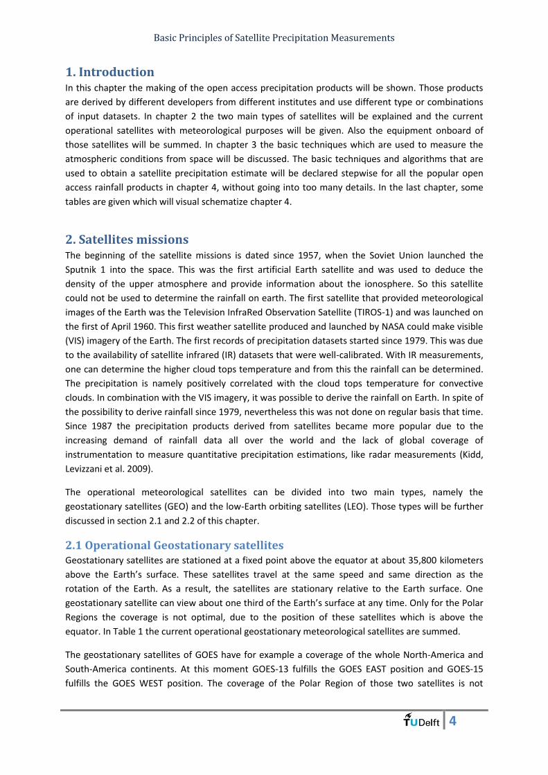
Basic Principles of Satellite Precipitation Measurements

4

1. Introduction In this chapter the making of the open access precipitation products will be shown. Those products

are derived by different developers from different institutes and use different type or combinations

of input datasets. In chapter 2 the two main types of satellites will be explained and the current

operational satellites with meteorological purposes will be given. Also the equipment onboard of

those satellites will be summed. In chapter 3 the basic techniques which are used to measure the

atmospheric conditions from space will be discussed. The basic techniques and algorithms that are

used to obtain a satellite precipitation estimate will be declared stepwise for all the popular open

access rainfall products in chapter 4, without going into too many details. In the last chapter, some

tables are given which will visual schematize chapter 4.

2. Satellites missions The beginning of the satellite missions is dated since 1957, when the Soviet Union launched the

Sputnik 1 into the space. This was the first artificial Earth satellite and was used to deduce the

density of the upper atmosphere and provide information about the ionosphere. So this satellite

could not be used to determine the rainfall on earth. The first satellite that provided meteorological

images of the Earth was the Television InfraRed Observation Satellite (TIROS-1) and was launched on

the first of April 1960. This first weather satellite produced and launched by NASA could make visible

(VIS) imagery of the Earth. The first records of precipitation datasets started since 1979. This was due

to the availability of satellite infrared (IR) datasets that were well-calibrated. With IR measurements,

one can determine the higher cloud tops temperature and from this the rainfall can be determined.

The precipitation is namely positively correlated with the cloud tops temperature for convective

clouds. In combination with the VIS imagery, it was possible to derive the rainfall on Earth. In spite of

the possibility to derive rainfall since 1979, nevertheless this was not done on regular basis that time.

Since 1987 the precipitation products derived from satellites became more popular due to the

increasing demand of rainfall data all over the world and the lack of global coverage of

instrumentation to measure quantitative precipitation estimations, like radar measurements (Kidd,

Levizzani et al. 2009).

The operational meteorological satellites can be divided into two main types, namely the

geostationary satellites (GEO) and the low-Earth orbiting satellites (LEO). Those types will be further

discussed in section 2.1 and 2.2 of this chapter.

2.1 Operational Geostationary satellites Geostationary satellites are stationed at a fixed point above the equator at about 35,800 kilometers

above the Earth’s surface. These satellites travel at the same speed and same direction as the

rotation of the Earth. As a result, the satellites are stationary relative to the Earth surface. One

geostationary satellite can view about one third of the Earth’s surface at any time. Only for the Polar

Regions the coverage is not optimal, due to the position of these satellites which is above the

equator. In Table 1 the current operational geostationary meteorological satellites are summed.

The geostationary satellites of GOES have for example a coverage of the whole North-America and

South-America continents. At this moment GOES-13 fulfills the GOES EAST position and GOES-15

fulfills the GOES WEST position. The coverage of the Polar Region of those two satellites is not

Basic Principles of Satellite Precipitation Measurements

5

optimal; this is also shown in Figure 1. Imagery obtained from geostationary satellites is primarily VIS

and IR, those techniques will be discussed in the next chapter (Kidd, Levizzani et al. 2009).

Table 1: Current Operational Geostationary Meteorological satellites in May 2014

Operator Satellite Position Launched/ End of life (expected)

Instruments for measuring precipitation (see also Table 3)

JMA (Japan) MTSAT-2 145° E 2010/2015 -

CMA/NRSCC FY-2D 86.5° E 2006/2014 S-VISSR

FY-2E 105° E 2004/2014 S-VISSR

FY-2F 112° E 2012/2016 S-VISSR/SXM

ISRO INSAT-3A 93.5° E 2003/2015 VHRR

INSAT-3D 82° E 2013/2021 IMAGER/SOUNDER

ISRO/IMD KALPANA-1 74° E 2002/2014 VHRR

RosHydroMet/ Roscosmos

ELECTRO-L N1 76° E 2011/2018 GGAK-E(SKIF-6)/ GGAK-E(SKIF-E)/ GGAK-E(GALS-E)/ GGAK-E(ISP-2M)/ GGAK-E(VUSS-E)/ GGAK-E(FM-E)/ GGAK-E(DIR-E)

EUMETSAT/ESA Meteosat-7 57.3° E 2006-2016 MVIRI

Meteosat-8 3.6° E 2002/2016 SEVIRI

Meteosat-9 9.4° E 2005/2019 SEVIRI

Meteosat-10 0° 2012/2019 SEVIRI

NASA/NOAA GOES-13 75° W 2006/2015 SOUNDER/IMAGER

GOES-14 105° W 2009/2016 SOUNDER/IMAGER

GOES-15 135° W 2010/2020 SOUNDER/IMAGER

Figure 1: Coverage of the GOES geostationary meteorological satellites (GOES 2014)

2.2 Operational Low orbiting satellites The second satellite category is the Low-Earth orbiting satellites (LEO). They are located 850Km

above the Earth’s surface and do not have a fixed point. The orbits are such that they cross the

Equator at the same local time. They fly around the Earth in about 100 minutes and are capable to

make a scan of all the areas of the world, so also the Polar Regions. A list of LEO satellites is given in

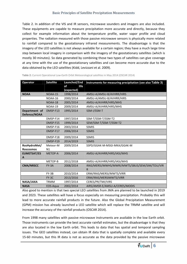
Basic Principles of Satellite Precipitation Measurements

6

Table 2. In addition of the VIS and IR sensors, microwave sounders and imagers are also included.

These equipments are capable to measure precipitation more accurate and directly, because they

collect for example information about the temperature profile, water vapor profile and cloud

properties. The radiation measured with those passive microwave sensors is physically more related

to rainfall compared to the geostationary infrared measurements. The disadvantage is that the

imagery of the LEO satellites is not always available for a certain region; they have a much large time

step between local imagery in comparison with the imagery of the geostationary satellites (which is

mostly 30 minutes). So data generated by combining those two types of satellites can give coverage

at any time with the use of the geostationary satellites and can become more accurate due to the

data obtained by the LEO satellites (Kidd, Levizzani et al. 2009).

Table 2: Current Operational Low-Earth Orbit Meteorological satellites in May 2014 (OSCAR 2014)

Operator Satellite Launched/End of life (expected)

Instruments for measuring precipitation (see also Table 3)

NOAA NOAA-15 1998/2014 AMSU-A/AMSU-B/AVHRR/HIRS

NOAA-16 2000/2014 AMSU-A/AMSU-B/AVHRR/HIRS

NOAA-18 2005/2014 AMSU-A/AVHRR/HIRS/MHS

NOAA-19 2009/2014 AMSU-A/AVHRR/HIRS/MHS

Department of Defence/NOAA

DMSP-F13 1995/2014 SSM-I/SSM-T

DMSP-F14 1997/2014 SSM-T/SSM-T/SSM-T2

DMSP-F15 1999/2014 SEM/SSM-T/SSM-T/SSM-T2

DMSP-F16 2003/2014 SSMIS

DMSP-F17 2006/2014 SSMIS

DMSP-F18 2009/2014 SSMIS

DMSP-F19 2014/2019 SSMIS

RosHydroMet/Roscosmos

Meteor-M N1

2009/2014 SSPD/GGAK-M-MSGI-MKA/GGAK-M

EUMETSAT/ESA

METOP-A 2006/2014 AMSU-A/AVHRR/HIRS/IASI/MHS

METOP-B 2012/2018 AMSU-A/AVHRR/HIRS/IASI/MHS

CMA/NRSCC FY-3A 2008/2014 IRAS/MERSI/MWHS/MWRI/MWTS/SBUS/SEM/SIM/TOU/VIRR

FY-3B 2010/2014 ERM/IRAS/MERSI/MWTS/VIRR

FY-3C 2013/2016 ERM/IRAS/MERSIMWTS/VIRR

NASA/JAXA TRMM 1997/2014 CERES/PR/TMI/VIRS

NASA EOS-Aqua 2002/2014 AIRS/AMSR-E/AMSU-A/CERES/MODIS

Also good to mention is that two special LEO satellites from JMA are planned to be launched in 2019

and 2023. These satellites will have a focus especially on measuring precipitation. Probably this will

lead to more accurate rainfall products in the future. Also the Global Precipitation Measurement

(GPM) mission has already launched a LEO satellite which will replace the TRMM satellite and will

increase the accuracy of the rainfall products (OSCAR 2014).

From 1998 many satellites with passive microwave instruments are available in the low Earth orbit.

Those instruments can provide the best accurate rainfall estimates, but the disadvantage is that they

are also located in the low Earth orbit. This leads to data that has spatial and temporal sampling

issues. The GEO satellites instead, can obtain IR data that is spatially complete and available every

15-60 minutes, but this IR data is not as accurate as the data provided by the passive microwave

Basic Principles of Satellite Precipitation Measurements

7

instruments. This situation has led to the development of different methods and algorithms to

combine the datasets from the GEO and LEO satellites and sometimes also ground measurements, to

obtain a satellite-based rainfall estimate product. The basic techniques for estimation the

precipitation will be discussed in the next chapter.

Table 3: List of instruments and its abbreviation used for precipitation measurements (OSCAR 2014)

List of instruments and its abbreviation: AIRS= Atmospheric Infra-Red Sounder AMSU-A= Advanced Microwave Sounding Unit -A AMSU-B= Advanced Microwave Sounding Unit –B AMSR-E= Advanced Microwave Scanning Radiometer for EOS AVHRR= Advanced Very High Resolution Radiometer CERES= Clouds and the Earth’s Radiant Energy System GGAK-M-KGI-4C= GGAK-M / Radiation Monitoring System GGAK-E(SKIF-6)= GGAK-E/Corpuscular radiation spectrometer GGAK-E(SKIF-E) = GGAK-E/Solar cosmic rays spectrometer GGAK-E(GALS-E)= GGAK-E/Detector of galactic cosmic rays GGAK-E(ISP-2M)= GGAK-E/Solar constant sensor GGAK-E(VUSS-E)= GGAK-E/Solar UV radiation sensor GGAK-E(FM-E)= GGAK-E/Magnetometer instrument GGAK-E(DIR-E)= Solar X-ray radiation flux sensor HIRS=High-resolution Infra Red Sounder IASI= Infrared Atmospheric Sounding Interferometer IMAGER=INSAT imager IRAS= Infra Red Atmospheric Sounder KMSS= High Resolution VIS/IR Radiometer

MERSI= Medium Resolution Spectral Imager MHS= Microwave Humidity Sounding MODIS= Moderate- resolution Imaging Spectro-radiometer MVIRI= Meteosat Visible Infra-Red Imager MWTS= Micro-Wave Temperature Sounder PR= Precipitation Radar SOUNDER= INSAT sounder SEVIRI= Spinning Enhanced Visible Infra-Red Imager SSM-I= Special Sensor Microwave - Imager SSM-T= Special Sensor Microwave – Temperature SSM-T2= Special Sensor Microwave – Humidity SSMIS= Special Sensor Microwave – Imager/Sounder SSPD= Data Collection and Transmission System S-VISSR= Stretched Visible and Infrared Spin Scan Radiometer TMI= TRMM Microwave Imager VHRR= Very High Resolution Radiometer VIRR= Visible and Infra-Red Radiometer VIRS= Visible and Infra Red Scanner

Basic Principles of Satellite Precipitation Measurements

8

3. Basic techniques In this part the basic techniques to obtain the datasets which are used to derive a satellite based

precipitation estimate will be discussed. In most of the precipitation product, techniques from

geostationary and low orbiting satellites are both used to get a combined precipitation estimates

which will increase the accuracy of the end product. The better accuracy is the result of the

combined advantages of both satellite techniques. All the techniques use different frequencies in

the electromagnetic spectrum. Firstly, the techniques of the geostationary satellites will be discussed

in section 3.1. In section 3.2, the techniques from the low orbiting satellites will be discussed. Those

techniques form the basis of the algorithms that are used to derive the precipitation products, but

there are several different algorithms for each technique to convert the measured electromagnetic

frequencies into precipitation estimations. Each satellite product uses a different set of algorithms to

transfer those frequencies into rainfall estimation.

3.1 Geostationary satellites As already mentioned, the advantage of this satellite is the spatial and temporal coverage of the

dataset. The whole world is covered for all time, because 1 satellite covers already a third of the total

surface of the earth. The disadvantage is the accuracy of the technique due to the large distance

between the satellite and the earth’s surface, this has an effects upon the frequencies that can be

used due to this distance (only VIS, NIR or TIR). So, only lower frequencies can be detected because

of the travel distance of those frequencies is larger. The relation between rainfall and those

frequencies is less accurate. Furthermore, the coverage of the polar regions is not optimal due to the

location of the satellite is above the equator (Kidd, Levizzani et al. 2009).

3.1.1 Passive microwave techniques

Passive microwave techniques are techniques which do not send a signal, but only detects an

electromagnetic signal with a certain frequency. This signal is emitted from the Earth surface or is

reflected sunlight by the Earth. The advantage is that less energy is needed to obtain a measurement,

this is especially ideal in space where a little amount of energy can be generated or stored.

Visible light technique

The most direct way to observe clouds is with the use of the visible part (VIS) of the electromagnetic

spectrum (frequencies between 430 and 790 THz). This results in an imagery which shows what we

would also observe with our own eyes. Clouds are relatively bright against the Earth’s black surface.

The brightness also depends on the thickness of the clouds. From the VIS images only, it is hard to

obtain the rain intensity, but they can provide useful information about the type of clouds. Those

imageries are only useful during daytime, when there is enough sunlight. During the night time no

clouds can be detected. The instruments used for those measurements are for example SEVIRI

sensors.

Near infrared technique

Near infrared channels (frequencies between 400 and 100 THz) are also very useful, because they

can provide information on the properties of the cloud top particles. The obtained data contains

information about the size of the cloud top particles and if the particles are liquid or ice. Those

channels are restricted to use only during daytime, because solar illumination is needed (Kidd,

Levizzani et al. 2009). SEVIRI sensor is an example of an instrument which can detect near infrared

frequencies.

Basic Principles of Satellite Precipitation Measurements

9

Infrared technique

The infrared technique (frequencies between 100 and 10 THz) uses a sensor which detects the

infrared frequencies which is emitted by the heat of the vapor inside the cloud top. From this

emitted frequency one can obtain the temperature of the cloud top. The rainfall estimation is based

upon the simple principle of: a colder cloud top contains more precipitable water resulting in higher

rainfall intensities. Those imageries are very useful in combination with the VIS and near IR imagery

to obtain precipitation. IR images are available during both day and night (Kidd, Levizzani et al. 2009).

The disadvantage is that relation between the measured IR radiance and the surface rainfall has a

relatively weak correlation and only detects deep convective rain events (Huffman, Adler et al. 1997).

Drizzle is difficult to detect when only the cloud top temperature is measured, because there is not a

clear temperature threshold between the distinction of rain or no rain. The instruments that can

measure IR are for example the SEVIRI sensor.

3.2 Low orbiting satellites Low orbiting satellites rainfall estimates can greatly increase the accuracy of the precipitation data

obtained from the GEO satellite. The only disadvantage is the spatial coverage of the LEO satellites.

The whole Earth cannot be covered by those satellites resulting in spatial gaps inside the data which

must be filled with other datasets or extrapolation techniques.

3.2.1 Passive microwave

The passive microwave sensors are also situated on low orbiting satellites. By detecting different

frequencies the precipitation estimations can be obtained with the use of a retrieval algorithm. The

scattering and emission techniques are the two most important techniques to retrieve rainfall from

the passive microwave sensors. Both will be described here.

Scattering technique

The basic scattering technique will be discussed here. In different products, different algorithms are

used to convert the measured frequencies into rainfall estimation. Those algorithms are described in

different papers, but the basic scattering technique remains the same. Scattering based rainfall

retrieval techniques use the scattering by ice particles at the rain cloud top. Larger amount of ice

particles associate with a heavier rainfall intensity. In order to obtain the scattering information,

frequencies of 50GHz or higher must be measured (Liu and Curry 1992). SSM-I, TMI, or MHS are

sensors which can measure those frequencies. Those sensors detect the scattering of the upwelling

radiation by precipitation sized ice particles within the rain layer. This technique can be used above

land and oceans. Some care must be taken to remove the errors because of strange scattering

features. Those errors are mostly located in deserts or snow surfaces.

Emission technique

Emission based techniques utilize the emission of the rain clouds. This technique is more accurate

than the scattering technique because they are more directly related to precipitation since the

thermal radiation that is emitted from liquid hydrometeors is sensed directly (Joyce, Xie et al. 2010).

More emission relates to higher rain intensity. The emitted radiation of rain clouds is more than the

radiation emitted by the background ocean and cloud free atmosphere (Liu and Curry 1992). Above

land, this technique is not applicable due to the large variation of the emitted radiation above land

surfaces. Frequencies of 50GHz or lower are used in the algorithm to obtain the emission based

rainfall estimation. The SSM-I, TMI, or AMSU-A are sensors which can detect those frequencies.

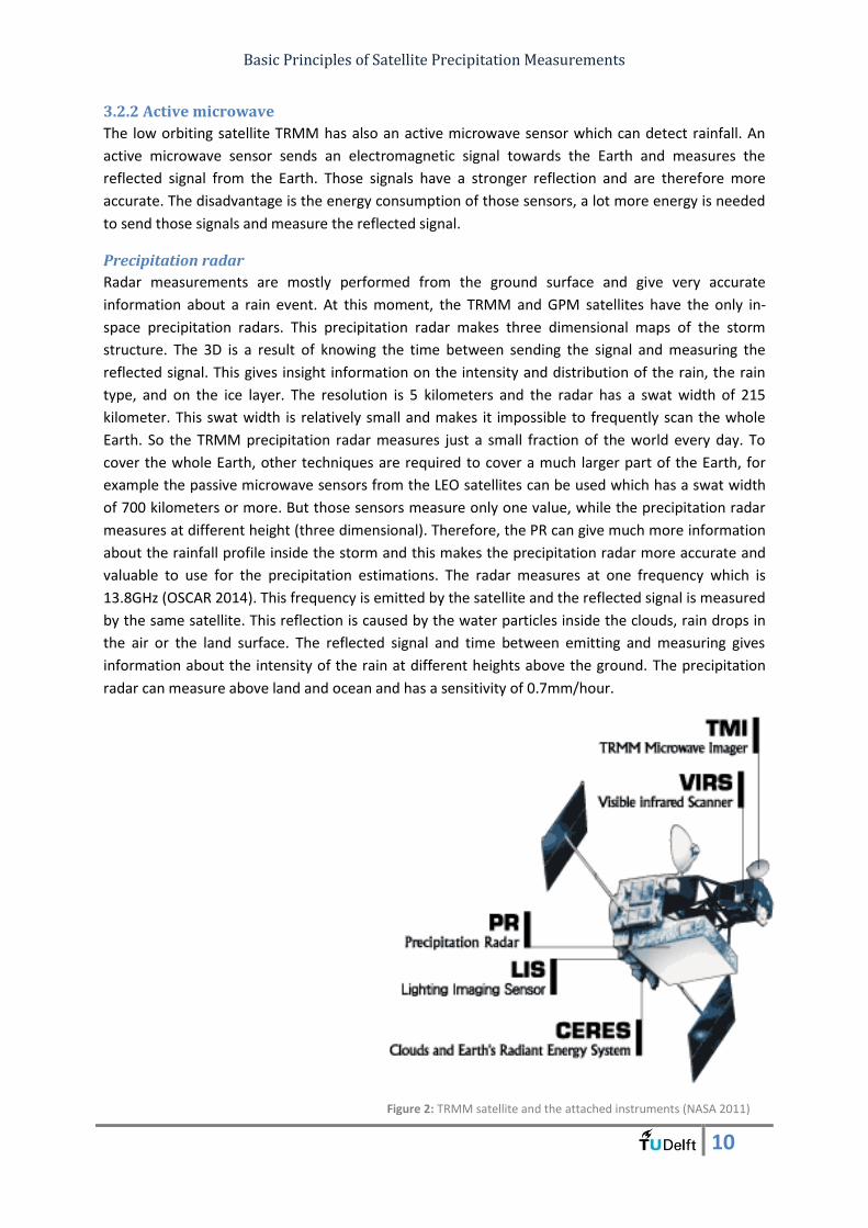
Basic Principles of Satellite Precipitation Measurements

10

3.2.2 Active microwave

The low orbiting satellite TRMM has also an active microwave sensor which can detect rainfall. An

active microwave sensor sends an electromagnetic signal towards the Earth and measures the

reflected signal from the Earth. Those signals have a stronger reflection and are therefore more

accurate. The disadvantage is the energy consumption of those sensors, a lot more energy is needed

to send those signals and measure the reflected signal.

Precipitation radar

Radar measurements are mostly performed from the ground surface and give very accurate

information about a rain event. At this moment, the TRMM and GPM satellites have the only in-

space precipitation radars. This precipitation radar makes three dimensional maps of the storm

structure. The 3D is a result of knowing the time between sending the signal and measuring the

reflected signal. This gives insight information on the intensity and distribution of the rain, the rain

type, and on the ice layer. The resolution is 5 kilometers and the radar has a swat width of 215

kilometer. This swat width is relatively small and makes it impossible to frequently scan the whole

Earth. So the TRMM precipitation radar measures just a small fraction of the world every day. To

cover the whole Earth, other techniques are required to cover a much larger part of the Earth, for

example the passive microwave sensors from the LEO satellites can be used which has a swat width

of 700 kilometers or more. But those sensors measure only one value, while the precipitation radar

measures at different height (three dimensional). Therefore, the PR can give much more information

about the rainfall profile inside the storm and this makes the precipitation radar more accurate and

valuable to use for the precipitation estimations. The radar measures at one frequency which is

13.8GHz (OSCAR 2014). This frequency is emitted by the satellite and the reflected signal is measured

by the same satellite. This reflection is caused by the water particles inside the clouds, rain drops in

the air or the land surface. The reflected signal and time between emitting and measuring gives

information about the intensity of the rain at different heights above the ground. The precipitation

radar can measure above land and ocean and has a sensitivity of 0.7mm/hour.

Figure 2: TRMM satellite and the attached instruments (NASA 2011)

Basic Principles of Satellite Precipitation Measurements

11

Basic Principles of Satellite Precipitation Measurements

12

4. Rainfall product algorithms This section will explain how the open access rainfall product developers produce the rainfall

datasets which are used in this research. All the popular open access rainfall products for Africa will

be explained one by one, because all the developers use different types of algorithms and combine

different type of data from satellites and ground measurements to come up with a rainfall estimate.

4.1 TRMM 3B43 TRMM 3B43 is a product of the Tropical Rainfall Measuring Mission (TRMM) which is a joint space

mission of the NASA and the Japan Aerospace Exploration Agency (JAXA). The main objective of this

mission is to monitor and study the tropical rainfall.

Table 4: Characteristics of the TRMM 3B43 rainfall product

TRMM 3B43

Input sensor satellite/ Retrieval Algorithm TMI and PR/TCI TMI/GPROF AMSR-E/GPROF SSM-I/GPROF MHS/NESDIS AMSU/NESDIS GEO-IR/VAR LEO-IR/VAR

Input gauge Yes (Monthly rain gauge/GPCC)

Spatial Scale, extent 0.25° x 0.25°, 0°E-360°E/50°N-50°S

Temporal scale, extent 3 hourly, 1 January 1998-present

TRMM 3B43 rainfall product has the formal name “TRMM and Other Data Precipitation Data Set”.

The applied algorithm is the Version 7 TRMM Multi-Satellite Precipitation Analysis (TMPA). This

method depends on two different types of satellite sensors as input data, namely microwave and IR

measurements (Huffman, Adler et al. 2010). The microwave data are obtained by a variety of LEO

satellites, including the TMI from the TRMM satellite, SSM-I from the DMSP satellites AMSR-E from

Aqua satellite, AMSU and MHS from the NOAA and METOP satellites. The Precipitation Radar (PR) is

also used from the TRMM satellite, which can provide three-dimensional maps of storm structure as

discussed before. In the beginning of the TRMM 3B43 dataset, there were only 3 LEO satellites

available. Thereby, only 40% of the Earth’s surface was covered by a microwave dataset. Nowadays,

this coverage problem is already improved due to the increasing amount of LEO satellites in space.

Furthermore, some new sensors are in the process of being involved into the TMPA, for example the

SSMIS from the DMSP F16 and F17 satellites and MHS from the NOAA 18 and METOP satellites to

improve the coverage. Another problem was malfunctioning of the instruments during some periods

of time, leading to a data gaps inside the continuous data, which leads to the availability of less data

for the TMPA for some periods. First, the algorithms for obtaining the precipitation data from the

different measured radiances will be discussed. In 4.1.4 the TMPA principle will be declared, this

principle combines the different rainfall datasets to obtain a combined precipitation product which

will improve the accuracy of the product a lot.

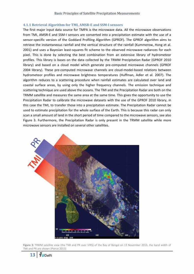
Basic Principles of Satellite Precipitation Measurements

13

4.1.1 Retrieval Algorithm for TMI, AMSR-E and SSM-I sensors

The first major input data source for TMPA is the microwave data. All the microwave observations

from TMI, AMSR-E and SSM-I sensors are converted into a precipitation estimate with the use of a

sensor-specific version of the Goddard Profiling Algorithm (GPROF). The GPROF algorithm aims to

retrieve the instantaneous rainfall and the vertical structure of the rainfall (Kummerow, Hong et al.

2001) and uses a Bayesian least-squares fit scheme to the observed microwave radiances for each

pixel. This is done by selecting the best combination from an extensive library of hydrometeor

profiles. This library is bases on the data collected by the TRMM Precipitation Radar (GPROF 2010

library) and based on a cloud model which generate pre-computed microwave channels (GPROF

2004 library). These pre-computed microwave channels are cloud-model-based relations between

hydrometeor profiles and microwave brightness temperatures (Huffman, Adler et al. 2007). The

algorithm reduces to a scattering procedure when rainfall estimates are calculated over land and

coastal surface areas, by using only the higher frequency channels. The emission technique and

scattering technique are used above the oceans. The TMI and the Precipitation Radar are both on the

TRMM satellite and measures the same area at the same time. This gives the opportunity to use the

Precipitation Radar to calibrate the microwave datasets with the use of the GPROF 2010 library, in

this case the TMI, to transfer those into a precipitation estimate. The Precipitation Radar cannot be

used to estimate precipitation for the whole surface of the Earth. This is because this radar can only

scan a small amount of land in the short period of time compared to the microwave sensors, see also

Figure 3. Furthermore, the Precipitation Radar is only present in the TRMM satellite while more

microwave sensors are installed on several other satellites.

Figure 3: TRMM satellite view (the TMI and PR over VIRS) of the Bay of Bengal on 13 November 2013, the band width of TMI and PR are shown (Pierce 2013)

Basic Principles of Satellite Precipitation Measurements

14

Another advantage of the passive microwave sensors is that they use a small amount of energy,

which is very useful when measuring in space. During the processing of the microwave data, they are

screened for contamination by surface effects. The objectives of this algorithm, is the providing of

instantaneous rainfall rates, the vertical structure of precipitation, and the associated latent heating

(Kummerow, Hong et al. 2001). A NESDIS algorithm is used to obtain the rainfall estimates from the

AMSU-B and MHS sensors. This algorithm also exist for the SSM-I sensor, but in the TMPA the GPROF

algorithm is used for this sensor, because of better results. The GPROF algorithm for SSM-I sensor

was modified to produce rainfall rates similar to those of the NESDIS rainfall algorithm, which will be

explained in the CMORPH section.

4.1.2 Retrieval Algorithm for AMSU-B and MHS sensors

The operational versions of the Zhao and Weng algorithm as described in their papers (Zhao and

Weng 2002, Weng, Zhao et al. 2003), convert the microwave observations from AMSU-B and MHS

into precipitation estimates. This algorithm is based on the scattering technique and is used by the

National Environmental Satellite Data and Information Service (NESDIS). The algorithm performs a

physical retrieval of ice water path (with the use of the 89GHz and 150GHz channel). The

convergence to the rain rate is made based on cloud data from the fifth-generation Pennsylvania

State University-National Center for Atmospheric Research (NCAR) Mesoscale Model (MM5) and also

on comparisons with in situ data (Joyce, Janowiak et al. 2004). The MM5 model is an empirically

derived relationship between retrieved ice amounts in the rain layer and in the tops of convective

clouds to actual surface rain. This scattering technique is used above land and ocean surfaces. But is

not the most accurate in comparison with the rain rate obtained with the GPROF algorithm from the

other passive microwave sensors. In contrast with the GPROF, the NESDIS do not retrieve the vertical

rainfall structure and do not use one of the GPROF’s libraries. The NESDIS algorithm is also further

discussed in the CMORPH section which makes use of the NESDIS algorithm also.

4.1.3 Retrieval Algorithm for the IR data

The second major data source for TMPA is the GEO-IR data. The advantage of this data source is the

time and space coverage. The GEO satellites can provide data for the whole Earth’s surface at any

time. The IR sensor use thermal IR to measure the cloud-top temperature in order to estimate

precipitation. However, the correlation between the cloud-top temperature and the precipitation is

very poorly at fine time and space scales, but relatively well correlated if a larger time and space

scale is used. With a daily time scale and a space scale of 2.5° x 2.5° the correlation is improved a lot

(Arkin and Meisner 1987). The Climate Prediction Center (CPC) merges the GEO-IR data into grids of 4

kilometers. The dataset is corrected for zenith-angle viewing effects and inter-satellite calibration

difference.

4.1.4 Combining products with TMPA

The TMPA employs three additional data sources, including TRMM Combined instruments (TCI)

estimates, this estimation results in the TRMM 2B31 product and combines data from the TMI and

the Precipitation Radar. The TMPA is computed in four stages:

1. The microwave precipitation estimates are inter-calibrated and combined

2. Providing IR precipitation estimates using the calibrated microwave precipitation

3. The microwave and IR rainfall estimations are combined

4. Gauged rainfall data are integrated

Basic Principles of Satellite Precipitation Measurements

15

Step 1:

All the microwave datasets are averaged to a 0.25° spatial grid over a +/- 90 minutes time range from

the nominal 3 hourly observation times. The best data source to adopt in the calibration is the TCI

data source. Which is a multi-sensor based data by combining the TMI and the Precipitation Radar of

the TRMM satellite. By applying the TCI-TMI calibration, one can use the TMI coverage to calibrate

other sensors from other satellites. This is needed because the coincidence of TCI coverage with any

of the sensors other than TMI is sparse. The TMI calibrations of the other microwave sensors are

adequately represented by climatologically-based coefficients representing large areas (Huffman,

Adler et al. 2010). Some calibrations are given separate climatologically adjustment one for land and

another for the oceans (for example the TMI-AMSR-E and the TMI-AMSU/MHS calibrations) and the

TMI-SSM/I calibration uses separate calibrations for five oceanic latitude bands. The TCI-adjusted

AMSU/MHS calibration has some additional issues in detectability deficiency over land.

The TMI calibration results in microwave estimates which are all calibrated for each sensor on several

satellites. From all these calibrated rainfall data, a single rainfall map is obtained. This map called the

High Quality (HQ) microwave combination field uses the best available microwave rainfall data. The

sequence of the best data is as follows, firstly the TCI data, if this data is not present for a grid than

the TCI-adjusted TMI, AMSR-E, SSM/I and SSMIS are used. So, only TCI is used if available. Otherwise,

all the TCI-adjusted data are used and averaged if necessary. The TCI-adjusted AMSU/MHS estimates

are only used if none of the other microwave estimates are available.

Step 2:

In this step the IR data are rescaled to the 0.25° spatial resolution. To do this, some pre-processing is

required. Full coverage of IR cloud top temperature is provided for the 3-hourly synoptic times. The

passive microwave data is used to calibrate the IR data. The calibration goes as follows: First, the IR

cloud top temperatures and the time-space matched HQ precipitation rates are accumulated for a

month into histograms. The data that is used for this monthly histogram are the 3 hourly values with

a spatial resolution of 0.25°x0.25° values on a 1°x1° target grid, aggregated to overlapping 3°x3°

windows with the 1°x1° target grid in the middle. This window is used to convert IR cloud top

temperature to precipitation rates (Huffman, Adler et al. 2007). The transformation into precipitation

rates is just the “colder the cloud the more precipitation” principle, so the coldest 0.25° x 0.25°

averaged cloud top temperature gets the greatest observed HQ precipitation rate. The result is a

spatially varying threshold value that is determined by the fractional coverage of precipitation for the

microwave data. A cloud top temperature warmer than this threshold will be assigned with zero

precipitation. This approach is also called the VAriable Rainrate (VAR) algorithm. If a grid has a lack of

coincident data throughout the month mainly due to cold-land dropouts or quality control, a

smooth-filled algorithm is applied which uses coincident data from surrounding grid boxes. The HQ-

IR calibration coefficients computed for a month are used for the 3 hourly IR dataset during that

month (Huffman, Adler et al. 2010). Those coefficients are used to improve the bias of the IR data.

This calibrated IR data is used when the passive microwave data is not available.

Step 3:

The next step is combining the HQ and IR precipitation estimates. The HQ estimates are used where

possible and the remaining grid boxes are filled with the HQ-calibrated IR estimates, see also Figure

4.

Basic Principles of Satellite Precipitation Measurements

16

Step 4:

In the last step the monthly rainfall gauge are introduced. The rain-gauge data are provided by the

Global Precipitation Climatological Center (GPCC) and by the Climate Assessment and Monitoring

System (CAMS). First, all the 3 hourly merged HQ-IR estimates are summed over the month. The

result is the monthly-satellite (MS) product. The MS and the gauge are combined by using inverse-

error-variance weighting to create a post-real-time monthly satellite-gauge combination (SG). For all

grids the SG/MG ratio is determined and then applied to scale each 3 hourly field in the month. The

fields have the details of the satellite data, but have nearly neutral monthly bias compared to gauges

(Huffman, Adler et al. 2007). All the TMPA steps are clearly visualized in the block diagram shown in

Figure 5.

Figure 4: Top: TRMM Precipitation Radar (PR) orbits in one day; Middle: Infrared data from TRMM Visible and Infrared Scanner (VIRS) orbits in one day; Bottom: NOAA NCEP Global IR image merged from five geostationary satellites (Negri, Adler et al. 2003).

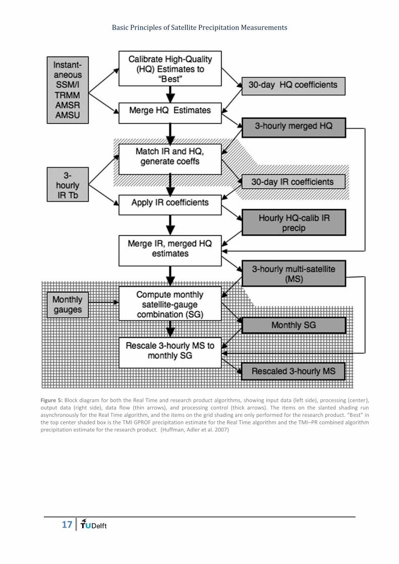
Basic Principles of Satellite Precipitation Measurements

17

Figure 5: Block diagram for both the Real Time and research product algorithms, showing input data (left side), processing (center), output data (right side), data flow (thin arrows), and processing control (thick arrows). The items on the slanted shading run asynchronously for the Real Time algorithm, and the items on the grid shading are only performed for the research product. “Best” in the top center shaded box is the TMI GPROF precipitation estimate for the Real Time algorithm and the TMI–PR combined algorithm precipitation estimate for the research product. (Huffman, Adler et al. 2007)

Basic Principles of Satellite Precipitation Measurements

18

4.2 CMORPH CMORPH stands for the Climate Prediction Center (CPC) morphing method and is a product that was

developed to combine the desirable aspect of the accuracy of the passive microwave and the spatial

and temporal coverage of the IR data. The IR data is only used to analyze the cloud movements and

the microwave data is used to derive all the rainfall estimates. So by using the motion of the clouds,

one can get insight in the propagation of the passive microwave based derived rainfall estimation for

each half hour for the whole Earth. The microwave data that is used are the SSM-I from the FY-13

satellite, SSMIS from the FY-16 and the DMSP satellites, the AMSR-E from the aqua satellite, the TMI

from the TRMM satellite, and the AMSU-B from the NOAA satellites. The NESDIS algorithm is used to

convert the brightness temperature measured with the AMSU sensor in a rainfall estimate and the

GPROF algorithm is used for the TMI sensor. The GPROF algorithm is already discussed in the TRMM

section. So only the NESDIS algorithm for the SSM-I/SSMIS sensor will be discussed here.

Table 5: Characteristics of the CMORPH rainfall product

CMORPH

Input sensor satellite/ Retrieval Algorithm TMI/GPROF SSMIS/NESDIS AMSR-E/NESDIS AMSU/NESDIS GEO-IR

Input gauge No

Spatial Scale, extent 0.25° x 0.25°, 0°E-360°E/60°N-60°S

Temporal scale, extent 3 hours, December 2002 - present

4.2.1 Retrieval Algorithm for SSM-I/SSMIS sensor

The NESDIS algorithm for the SSM-I/SSMIS is a scattering technique which is applicable over land and

ocean. The rain rate is derived with an empirical relationship between the ice amount (which is

formed inside the rain layer or in the tops of convective clouds) and the actual surface rainfall. With

this relation one can estimate the precipitation amounts, because more scattering due to larger or

more ice particles relates to higher rain intensities (Joyce, Janowiak et al. 2004). This scattering

technique is used above land and ocean surfaces and uses the higher frequencies (89- or 150-GHz

channel). Furthermore, an additional algorithm provides rainfall estimates over ocean surfaces with a

method that is based upon the absorption of the upwelling radiation by rain and cloud water by

using the lower frequency bands (19-,22- and 37-GHz) (Joyce, Xie et al. 2010). This technique is called

the emission technique as discussed earlier. The rainfall estimates obtained from these thermal

emission channels are more accurate than the estimates from the scattering techniques because the

relationship between the emission and rainfall is more direct. The lower frequencies used in the

emission technique are not measurable with the AMSU-B sensor, but can be measured with the SSM-

I and MTI sensors. The use of these additional frequencies channels makes the estimated rain rate

for the oceans a lot more accurate. Also the AMSR-E can detect the scattering and emission

signatures.

4.2.2 Normalization of the microwave derived precipitation estimates

The rainfall estimations based on the SSM-I, AMSR-E and TMI sensors are similar, this is because

those sensors are equipped with channels that can detect scattering and emission signatures.

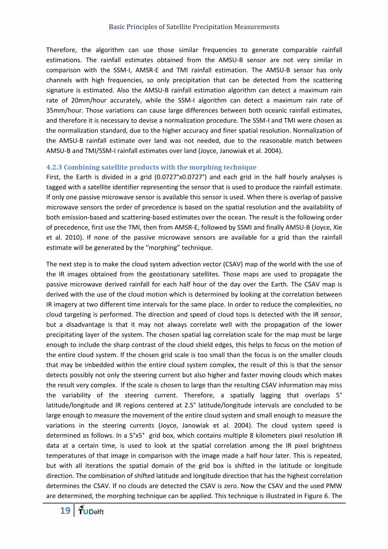
Basic Principles of Satellite Precipitation Measurements

19

Therefore, the algorithm can use those similar frequencies to generate comparable rainfall

estimations. The rainfall estimates obtained from the AMSU-B sensor are not very similar in

comparison with the SSM-I, AMSR-E and TMI rainfall estimation. The AMSU-B sensor has only

channels with high frequencies, so only precipitation that can be detected from the scattering

signature is estimated. Also the AMSU-B rainfall estimation algorithm can detect a maximum rain

rate of 20mm/hour accurately, while the SSM-I algorithm can detect a maximum rain rate of

35mm/hour. Those variations can cause large differences between both oceanic rainfall estimates,

and therefore it is necessary to devise a normalization procedure. The SSM-I and TMI were chosen as

the normalization standard, due to the higher accuracy and finer spatial resolution. Normalization of

the AMSU-B rainfall estimate over land was not needed, due to the reasonable match between

AMSU-B and TMI/SSM-I rainfall estimates over land (Joyce, Janowiak et al. 2004).

4.2.3 Combining satellite products with the morphing technique

First, the Earth is divided in a grid (0.0727°x0.0727°) and each grid in the half hourly analyses is

tagged with a satellite identifier representing the sensor that is used to produce the rainfall estimate.

If only one passive microwave sensor is available this sensor is used. When there is overlap of passive

microwave sensors the order of precedence is based on the spatial resolution and the availability of

both emission-based and scattering-based estimates over the ocean. The result is the following order

of precedence, first use the TMI, then from AMSR-E, followed by SSMI and finally AMSU-B (Joyce, Xie

et al. 2010). If none of the passive microwave sensors are available for a grid than the rainfall

estimate will be generated by the “morphing” technique.

The next step is to make the cloud system advection vector (CSAV) map of the world with the use of

the IR images obtained from the geostationary satellites. Those maps are used to propagate the

passive microwave derived rainfall for each half hour of the day over the Earth. The CSAV map is

derived with the use of the cloud motion which is determined by looking at the correlation between

IR imagery at two different time intervals for the same place. In order to reduce the complexities, no

cloud targeting is performed. The direction and speed of cloud tops is detected with the IR sensor,

but a disadvantage is that it may not always correlate well with the propagation of the lower

precipitating layer of the system. The chosen spatial lag correlation scale for the map must be large

enough to include the sharp contrast of the cloud shield edges, this helps to focus on the motion of

the entire cloud system. If the chosen grid scale is too small than the focus is on the smaller clouds

that may be imbedded within the entire cloud system complex, the result of this is that the sensor

detects possibly not only the steering current but also higher and faster moving clouds which makes

the result very complex. If the scale is chosen to large than the resulting CSAV information may miss

the variability of the steering current. Therefore, a spatially lagging that overlaps 5°

latitude/longitude and IR regions centered at 2.5° latitude/longitude intervals are concluded to be

large enough to measure the movement of the entire cloud system and small enough to measure the

variations in the steering currents (Joyce, Janowiak et al. 2004). The cloud system speed is

determined as follows. In a 5°x5° grid box, which contains multiple 8 kilometers pixel resolution IR

data at a certain time, is used to look at the spatial correlation among the IR pixel brightness

temperatures of that image in comparison with the image made a half hour later. This is repeated,

but with all iterations the spatial domain of the grid box is shifted in the latitude or longitude

direction. The combination of shifted latitude and longitude direction that has the highest correlation

determines the CSAV. If no clouds are detected the CSAV is zero. Now the CSAV and the used PMW

are determined, the morphing technique can be applied. This technique is illustrated in Figure 6. The

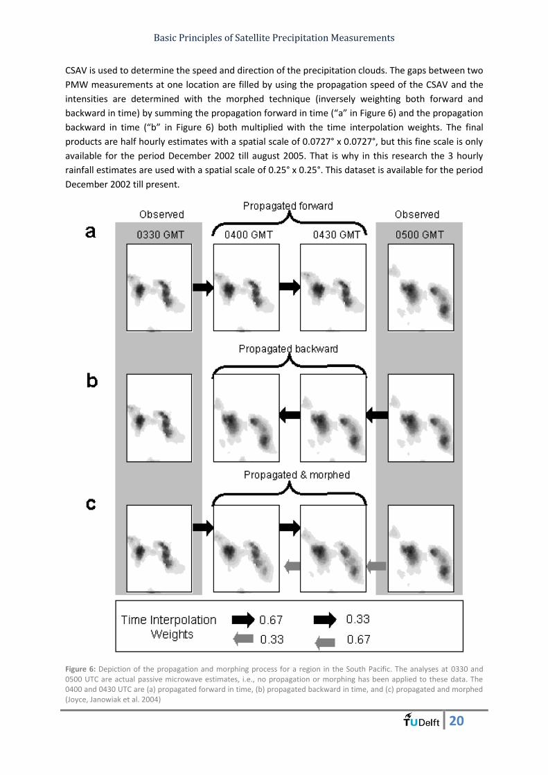
Basic Principles of Satellite Precipitation Measurements

20

CSAV is used to determine the speed and direction of the precipitation clouds. The gaps between two

PMW measurements at one location are filled by using the propagation speed of the CSAV and the

intensities are determined with the morphed technique (inversely weighting both forward and

backward in time) by summing the propagation forward in time (“a” in Figure 6) and the propagation

backward in time (“b” in Figure 6) both multiplied with the time interpolation weights. The final

products are half hourly estimates with a spatial scale of 0.0727° x 0.0727°, but this fine scale is only

available for the period December 2002 till august 2005. That is why in this research the 3 hourly

rainfall estimates are used with a spatial scale of 0.25° x 0.25°. This dataset is available for the period

December 2002 till present.

Figure 6: Depiction of the propagation and morphing process for a region in the South Pacific. The analyses at 0330 and 0500 UTC are actual passive microwave estimates, i.e., no propagation or morphing has been applied to these data. The 0400 and 0430 UTC are (a) propagated forward in time, (b) propagated backward in time, and (c) propagated and morphed (Joyce, Janowiak et al. 2004)

Basic Principles of Satellite Precipitation Measurements

21

4.3 GPCP V2.2 The Global Precipitation Climatology Project (GPCP) is a rainfall estimation dataset from 1979 till

present and combines ground observations and satellite precipitation data into 2.5°x2.5° global grids.

In order to produce this dataset it uses the SSM/I and SSMIS instruments from the DMSP satellites,

the AVHRR from the NOAA satellites, AIRS instruments from the AQUA satellite, the IR images of the

GEO satellites and the rain gauge data dataset from the GPCC.

Table 6: Characteristics of the GPCP V2.2 rainfall product

GPCP V2.2

Input sensor satellite/algorithm datasets SSMIS/Emission algorithm (Wilheit, Chang et al. 1991) and Scattering algorithm (Grody 1991) AIRS/Data processing (Susskind and Pfaendtner 1989, Susskind, Piraino et al. 1997) AVHRR/GPI GEO-IR/GPI

Input gauge Yes (Monthly rain gauge/GPCC)

Spatial Scale, extent 2.5° x 2.5°, 0°E-360°E/90°N-90°S

Temporal scale, extent Monthly, July 1987 - present

4.3.1 Retrieval Algorithm for the SSM-I/SSMIS and AIRS

For the SSM-I/SSMIS instruments two algorithms are used to obtain the rainfall estimates. One

algorithm is especially for the ocean parts and uses the lower frequencies bands (19 GHz, 22 GHz and

37 GHz channels). This algorithm is called the emission algorithm. The rainfall estimates obtained

from this algorithm are only reliable over the ocean because here the surface emissivity is low and

uniform. Above the land surfaces, the emissivity is higher and extremely heterogeneous, which

makes a rainfall estimation based upon the scattering algorithm a better choice. For the ice surfaces

the AIRS rainfall estimates is the best option.

The retrieval algorithm for the SSM-I/SSMIS emission based precipitation product uses the Wilheit et

al. (1991) histogram approach. This algorithm uses the 19GHz and 22GHz channels to determine the

rainfall amount by making a histogram in which the brightness temperature is plotted against the

number of occurrences. The used brightness temperature for the rainfall estimate is obtained by

taking two times the brightness temperature of the 19GHz channel minus the brightness

temperature of the 22GHz channel. This leads to a clear distinction between rain and no rain in the

brightness temperature histogram, because the histogram can be modeled by assuming a normal

distribution for no rain and a log normal distribution for rain. The parameters needed for the

distributions are obtained iteratively by comparing computed histogram with the observed

histogram. The modeled fit is applied to a histogram which exists of the full month of data. The rain

rate that corresponds to the intersection of the two distributions (normal and log normal) is typically

of the order of 0.5mm/hour. Also the freezing level (which is obtained from the 19GHz and the

22GHz channels) is used to derive the rain estimation. The flow chart of this process is also shown in

Figure 7. The individual rainfall estimates are determined for a 2.5°x2.5° grid (Wilheit, Chang et al.

1991).

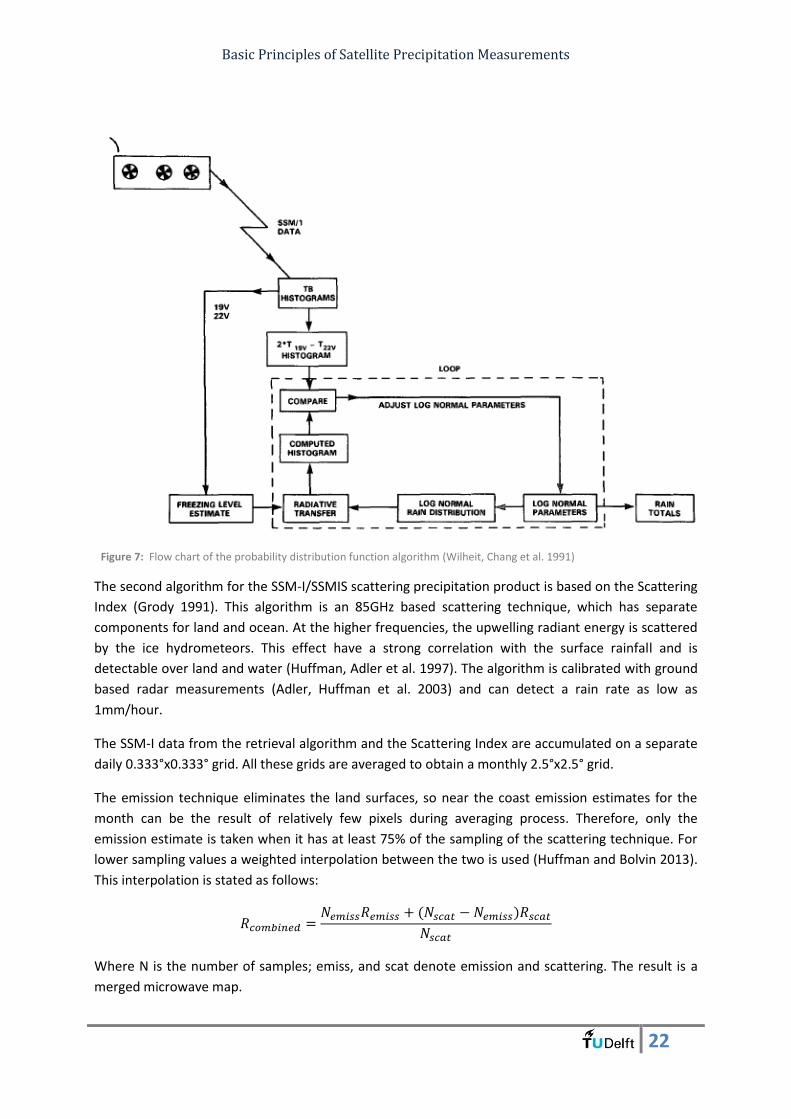
Basic Principles of Satellite Precipitation Measurements

22

The second algorithm for the SSM-I/SSMIS scattering precipitation product is based on the Scattering

Index (Grody 1991). This algorithm is an 85GHz based scattering technique, which has separate

components for land and ocean. At the higher frequencies, the upwelling radiant energy is scattered

by the ice hydrometeors. This effect have a strong correlation with the surface rainfall and is

detectable over land and water (Huffman, Adler et al. 1997). The algorithm is calibrated with ground

based radar measurements (Adler, Huffman et al. 2003) and can detect a rain rate as low as

1mm/hour.

The SSM-I data from the retrieval algorithm and the Scattering Index are accumulated on a separate

daily 0.333°x0.333° grid. All these grids are averaged to obtain a monthly 2.5°x2.5° grid.

The emission technique eliminates the land surfaces, so near the coast emission estimates for the

month can be the result of relatively few pixels during averaging process. Therefore, only the

emission estimate is taken when it has at least 75% of the sampling of the scattering technique. For

lower sampling values a weighted interpolation between the two is used (Huffman and Bolvin 2013).

This interpolation is stated as follows:

Where N is the number of samples; emiss, and scat denote emission and scattering. The result is a

merged microwave map.

Figure 7: Flow chart of the probability distribution function algorithm (Wilheit, Chang et al. 1991)

Basic Principles of Satellite Precipitation Measurements

23

For the ice covered surfaces of the Earth the AIRS rainfall estimates are the most optimal. Before the

AIRS data was available the TOVS data from the NOAA satellites were used. The same algorithm can

be applied for both datasets. This approach is described in several researches (Susskind and

Pfaendtner 1989, Susskind, Piraino et al. 1997). The merged precipitation product will be the

coverage of the SSM-I data (which is limited by the DMSP satellites orbits and measurements above

cold land surfaces) filled with globally complete AIRS data between the 40° North and South belt.

When moving more towards the poles, the SSM-I data becomes less reliable. Therefore just outside

this zone, the SSM-I and TOVS data are averaged by using equal weighting. And moving further

toward the poles the data is filled with TOVS data that have been adjusted to a zonal averaged

presumed bias (Huffman and Bolvin 2013).

4.3.2 Retrieval Algorithm for the IR estimates

The IR estimates are produced by the GEO satellites. The global IR precipitation estimates are derived

from a merger of these data using the GOES Precipitation Index (GPI) technique (Arkin and Meisner

1987). This simple technique gives a precipitation rate of 3mm/hour for cells with a brightness

temperature of 235K or lower. For higher brightness temperature a precipitation rate of 0 mm/hour

is assigned. From October 1996 till present, the GPI data are accumulated on 1°x1° grid every 3

hours. The gaps in the GEO IR data (part of the Indian Ocean until June 1998 and outside the 40°

North and South belt) are filled with the LEO IR (AVHRR) data from the NOAA polar orbiting satellites.

This LEO IR data is also converted into GPI estimates by using a procedure described in other

researches (Janowiak and Arkin 1991) but will not be discussed further here, because this technique

is only used for data from 1998 or older and not used for the modern precipitation estimations.

4.3.3 Obtaining the AGPI from the GPI

Now the microwave images are known and the GPI from the GEO IR and LEO IR are derived, one can

make the adjusted GPI (AGPI). The AGPI combines the microwave rainfall estimation obtained from

the Retrieval algorithm and the Scattering Index with the GPI rainfall estimation. The 3 hourly GPI

rainfall values that correspond most closely in time to the local overpass time of the microwave

rainfall values (from the merged SSM-I, SSMIS and AIRS precipitation estimates) are used to

determine the ratio between both. This will result in adjusted spatially varying coefficients which are

applied to the full set of GPI estimates. This procedure will reduce known biases in the IR estimates,

while the high sampling rate of the GEO satellites is retained. The GPI from the LEO IR (LEO AGPI) are

adjusted by using smoothly varying interpolation of the microwave-IR adjustment ratio (Adler,

Huffman et al. 2003), because not all the 3 hours in a month are covered by the LEO GPI rainfall

estimation or the SSM-I/SSMIS.

4.3.4 Combining satellite products to obtain GPCP

The AGPI, LEO AGPI and the microwave estimates are combined to get the multi satellite product.

First the GEO AGPI is used between the 40° North and South belt if they are available. If the GEO

AGPI is not available in this zone a weighted combination is used between the LEO AGPI and the

merged microwave rainfall estimations. The weights are determined by using the inverse error

variances of the respective estimates. This is done because the LEO IR has not enough sampling to

cover the whole surface. Outside the 40° North and South belt the merged microwave rainfall

estimates are used.

The last step is combining the rain gauge data collected by the GPCC. This dataset consist of more

than 70.000 stations around the Earth. The large scale (5x5 grid box) average of the multi satellite

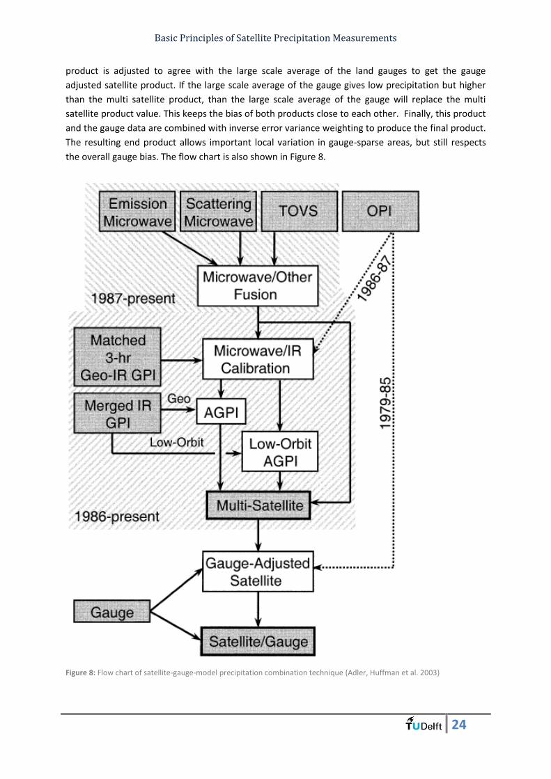
Basic Principles of Satellite Precipitation Measurements

24

product is adjusted to agree with the large scale average of the land gauges to get the gauge

adjusted satellite product. If the large scale average of the gauge gives low precipitation but higher

than the multi satellite product, than the large scale average of the gauge will replace the multi

satellite product value. This keeps the bias of both products close to each other. Finally, this product

and the gauge data are combined with inverse error variance weighting to produce the final product.

The resulting end product allows important local variation in gauge-sparse areas, but still respects

the overall gauge bias. The flow chart is also shown in Figure 8.

Figure 8: Flow chart of satellite-gauge-model precipitation combination technique (Adler, Huffman et al. 2003)

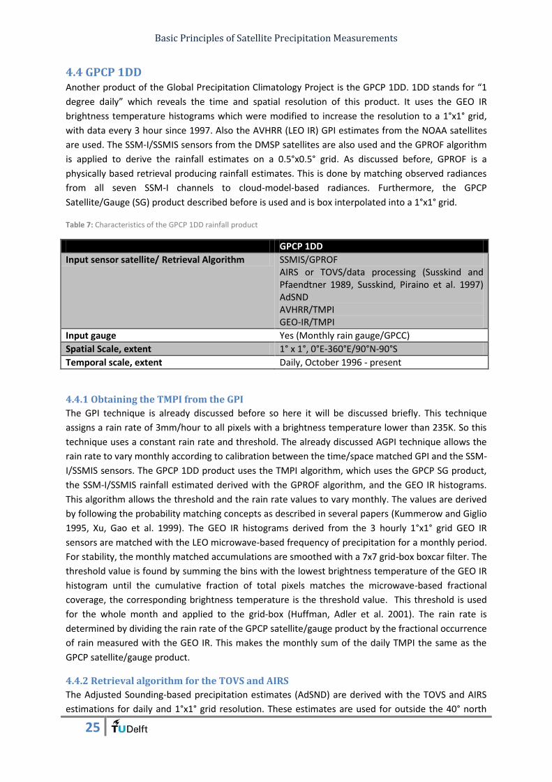
Basic Principles of Satellite Precipitation Measurements

25

4.4 GPCP 1DD Another product of the Global Precipitation Climatology Project is the GPCP 1DD. 1DD stands for “1

degree daily” which reveals the time and spatial resolution of this product. It uses the GEO IR

brightness temperature histograms which were modified to increase the resolution to a 1°x1° grid,

with data every 3 hour since 1997. Also the AVHRR (LEO IR) GPI estimates from the NOAA satellites

are used. The SSM-I/SSMIS sensors from the DMSP satellites are also used and the GPROF algorithm

is applied to derive the rainfall estimates on a 0.5°x0.5° grid. As discussed before, GPROF is a

physically based retrieval producing rainfall estimates. This is done by matching observed radiances

from all seven SSM-I channels to cloud-model-based radiances. Furthermore, the GPCP

Satellite/Gauge (SG) product described before is used and is box interpolated into a 1°x1° grid.

Table 7: Characteristics of the GPCP 1DD rainfall product

GPCP 1DD

Input sensor satellite/ Retrieval Algorithm SSMIS/GPROF AIRS or TOVS/data processing (Susskind and Pfaendtner 1989, Susskind, Piraino et al. 1997) AdSND AVHRR/TMPI GEO-IR/TMPI

Input gauge Yes (Monthly rain gauge/GPCC)

Spatial Scale, extent 1° x 1°, 0°E-360°E/90°N-90°S

Temporal scale, extent Daily, October 1996 - present

4.4.1 Obtaining the TMPI from the GPI

The GPI technique is already discussed before so here it will be discussed briefly. This technique

assigns a rain rate of 3mm/hour to all pixels with a brightness temperature lower than 235K. So this

technique uses a constant rain rate and threshold. The already discussed AGPI technique allows the

rain rate to vary monthly according to calibration between the time/space matched GPI and the SSM-

I/SSMIS sensors. The GPCP 1DD product uses the TMPI algorithm, which uses the GPCP SG product,

the SSM-I/SSMIS rainfall estimated derived with the GPROF algorithm, and the GEO IR histograms.

This algorithm allows the threshold and the rain rate values to vary monthly. The values are derived

by following the probability matching concepts as described in several papers (Kummerow and Giglio

1995, Xu, Gao et al. 1999). The GEO IR histograms derived from the 3 hourly 1°x1° grid GEO IR

sensors are matched with the LEO microwave-based frequency of precipitation for a monthly period.

For stability, the monthly matched accumulations are smoothed with a 7x7 grid-box boxcar filter. The

threshold value is found by summing the bins with the lowest brightness temperature of the GEO IR

histogram until the cumulative fraction of total pixels matches the microwave-based fractional

coverage, the corresponding brightness temperature is the threshold value. This threshold is used

for the whole month and applied to the grid-box (Huffman, Adler et al. 2001). The rain rate is

determined by dividing the rain rate of the GPCP satellite/gauge product by the fractional occurrence

of rain measured with the GEO IR. This makes the monthly sum of the daily TMPI the same as the

GPCP satellite/gauge product.

4.4.2 Retrieval algorithm for the TOVS and AIRS

The Adjusted Sounding-based precipitation estimates (AdSND) are derived with the TOVS and AIRS

estimations for daily and 1°x1° grid resolution. These estimates are used for outside the 40° north

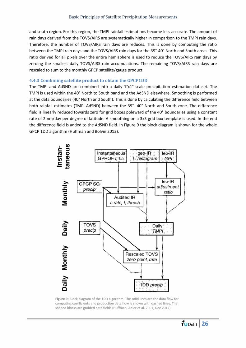
Basic Principles of Satellite Precipitation Measurements

26

and south region. For this region, the TMPI rainfall estimations become less accurate. The amount of

rain days derived from the TOVS/AIRS are systematically higher in comparison to the TMPI rain days.

Therefore, the number of TOVS/AIRS rain days are reduces. This is done by computing the ratio

between the TMPI rain days and the TOVS/AIRS rain days for the 39°-40° North and South areas. This

ratio derived for all pixels over the entire hemisphere is used to reduce the TOVS/AIRS rain days by

zeroing the smallest daily TOVS/AIRS rain accumulations. The remaining TOVS/AIRS rain days are

rescaled to sum to the monthly GPCP satellite/gauge product.

4.4.3 Combining satellite product to obtain the GPCP1DD

The TMPI and AdSND are combined into a daily 1°x1° scale precipitation estimation dataset. The

TMPI is used within the 40° North to South band and the AdSND elsewhere. Smoothing is performed

at the data boundaries (40° North and South). This is done by calculating the difference field between

both rainfall estimates (TMPI-AdSND) between the 39°- 40° North and South zone. The difference

field is linearly reduced towards zero for grid boxes poleward of the 40° boundaries using a constant

rate of 2mm/day per degree of latitude. A smoothing on a 3x3 grid box template is used. In the end

the difference field is added to the AdSND field. In Figure 9 the block diagram is shown for the whole

GPCP 1DD algorithm (Huffman and Bolvin 2013).

Figure 9: Block diagram of the 1DD algorithm. The solid lines are the data flow for computing coefficients and production data flow is shown with dashed lines. The shaded blocks are gridded data fields (Huffman, Adler et al. 2001, Dee 2012).

Basic Principles of Satellite Precipitation Measurements

27

4.5 PERSIANN PERSIANN is an abbreviation of Precipitation Estimation from Remotely Sensed Information using

Artificial Neural Networks and is developed at the University of Arizona. It uses the GEO IR

measurements as input for the adaptive Artificial Neural Network (ANN) model. To improve this

model independent estimates are provided by the TRMM 2A12 rain rate estimation to update the

network parameters. The input for the TRMM 2A12 rainfall estimates are obtained by using only the

TMI channels from the TRMM satellite converted with the GPROF algorithm. The TMI is chosen

because of the higher spatial resolution compared to the SSM-I sensors due to the lower orbit of the

TRMM spacecraft (Joyce, Xie et al. 2010). The end product is a half hourly product with a spatial

resolution of 0.25°x0.25°.

Table 8: Characteristics of the PERSIANN rainfall product

PERSIANN

Input sensor satellite/ Retrieval Algorithm TMI/GPROF GEO-IR/ANN

Input gauge No

Spatial Scale, extent 0.25° x 0.25°, 0°E-360°E/60°N-60°S

Temporal scale, extent 30 minutes, March 2000 - present

4.5.1 ANN model

An ANN model is used very often in various fields of technology and science, especially in fields which

involves time series forecasting, pattern recognition and process control. The structure is

mathematically proven to be an universal function approximator, which can map any complicated

nonlinear function to an arbitrary degree of accuracy (Hsu, Gao et al. 1997). The input for the ANN

model is obtained from the GEO satellites. A 5x5 pixel moving window is considered to derive rainfall

estimations for the central pixel of the moving window. So not only the target pixel is included, but

also at the surrounding pixels. The ANN model consists of two components, namely the SOFM and

the MGLL component. The SOFM component transfers the input IR data into the hidden layer and

the MGLL component transfers the hidden layer into an estimation of rainfall. Both components will

be discussed below.

4.5.1 SOFM

The Self Organizing Feature Map (SOFM) transfers the input IR data into the hidden layers (Kohonen

1982). The SOFM is used to classify the variables into a large number of groups (hidden nodes)

associated with different cloud surface characteristics (Sorooshian, Hsu et al. 2000). An important

requirement to get plausible rainfall estimations is the selection of input variables. These variables

must provide sufficient information to capture the cloud structure. But too many variables will make

the model too complicated. For the PERSIANN SOFM six input variables from the GEO IR satellite are

used. Those are shown in Table 9. In this table the first 2 variables give information about the target

pixel and the other variables give information about the cloud structural features. The SOFM make

an input-hidden layer transformation which performs an automatic clustering of the input space. The

hidden layer exists of a limited amount of hidden notes which all have a different variable vector, see

also Figure 10. The model looks at the six variables and places it in the hidden node which seems to

be the most comparable of all of the nodes in the hidden layer (the “winner” node). In the beginning

of the SOFM, the hidden layer must be trained. It uses the input variables to improve and update the

hidden layer by reorganizing the hidden notes so that their parameter vectors mimic the distribution

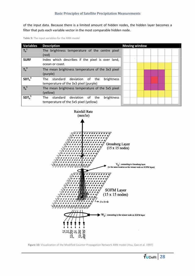
Basic Principles of Satellite Precipitation Measurements

28

of the input data. Because there is a limited amount of hidden nodes, the hidden layer becomes a

filter that puts each variable vector in the most comparable hidden node.

Table 9: The input variables for the ANN model

Variables Description Moving window

Tb1 The brightness temperature of the centre pixel

(red)

SURF Index which describes if the pixel is over land, ocean or coast.

Tb3 The mean brightness temperature of the 3x3 pixel

(purple)

SDTb3 The standard deviation of the brightness

temperature of the 3x3 pixel (purple)

Tb5 The mean brightness temperature of the 5x5 pixel

(yellow)

SDTb5 The standard deviation of the brightness

temperature of the 5x5 pixel (yellow)

Figure 10: Visualization of the Modified Counter Propagation Network ANN model (Hsu, Gao et al. 1997)

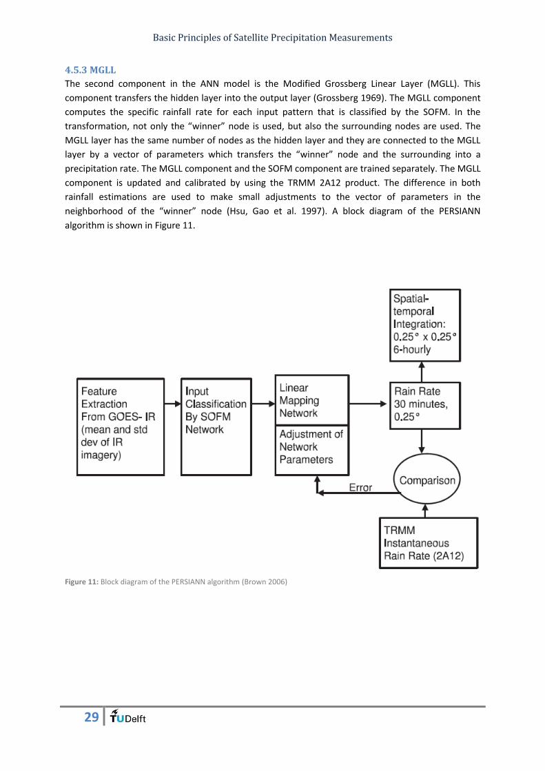
Basic Principles of Satellite Precipitation Measurements

29

4.5.3 MGLL

The second component in the ANN model is the Modified Grossberg Linear Layer (MGLL). This

component transfers the hidden layer into the output layer (Grossberg 1969). The MGLL component

computes the specific rainfall rate for each input pattern that is classified by the SOFM. In the

transformation, not only the “winner” node is used, but also the surrounding nodes are used. The

MGLL layer has the same number of nodes as the hidden layer and they are connected to the MGLL

layer by a vector of parameters which transfers the “winner” node and the surrounding into a

precipitation rate. The MGLL component and the SOFM component are trained separately. The MGLL

component is updated and calibrated by using the TRMM 2A12 product. The difference in both

rainfall estimations are used to make small adjustments to the vector of parameters in the

neighborhood of the “winner” node (Hsu, Gao et al. 1997). A block diagram of the PERSIANN

algorithm is shown in Figure 11.

Figure 11: Block diagram of the PERSIANN algorithm (Brown 2006)

Basic Principles of Satellite Precipitation Measurements

30

4.6 GSMaP GSMaP (Global Satellite Mapping of Precipitation) estimate precipitation rate on an hourly and a

global resolution. The spatial resolution is 0.1°x0.1°. This product uses the GEO IR sensors and a

handful of LEO passive microwave sensors. The used LEO passive microwave sensors are the SSM-I

from the DMSP satellites, the AMSR-E from the AQUA satellite and the TMI from the TRMM satellite.

Furthermore, the Precipitation Radar is used from the TRMM satellite. The algorithm to convert the

brightness temperature obtained from the LEO passive microwave sensors to surface rain is

described in several researches (Aonashi, Shibata et al. 1996, Kubota, Shige et al. 2007) and will be

briefly discussed below.

Table 10: Characteristics of the GSMaP rainfall product

GSMaP_MVK

Input sensor satellite/ Retrieval Algorithm PR/ GANAL TMI/Scattering algorithm (Aonashi, Shibata et al. 1996) SSMIS/ Scattering algorithm (Aonashi, Shibata et al. 1996) AMSR-E/Scattering algorithm (Aonashi, Shibata et al. 1996) GEO-IR

Input gauge No

Spatial Scale, extent 0.1° x 0.1°, 0°E-360°E/60°N-60°S

Temporal scale, extent hourly, May 2000 – November 2010

4.6.1 RTM algorithm for the GSMaP product

for the forward model

This algorithm tries to find the optimal

precipitation estimate which is when the Radiative

Transfer Model (RTM) field of view averaged

brightness temperature have the best fit with the

observed brightness temperature. This algorithm

exists of two parts. The flow chart of this algorithm

is shown in Figure 13. The left part, is the process of

making the lookup tables (LUTs) which shows the

relationship between rainfall rate and brightness

temperature. The LUTs for homogeneous

precipitation are calculated from forward

calculations with a four-stream RTM by linearly

interpolate the neighboring four boxes. These

tables are computed for a daily scale for a 5°x5°

grid and for all sensor frequencies. The input for

the RTM exist of atmospheric variables that are

given by the JMA Global Analysis (GANAL). The RTM

is classified by eight precipitation types and also

uses the Precipitation Radar as input for the

Figure 12: The LUT for the brightness temperature (Tb) and type 8 at a grid point on 1 January 1998. The solid lines are labeled and denote the value of precipitation inhomogeneity (Kubota, Shige et al. 2007)

Basic Principles of Satellite Precipitation Measurements

31

observed hydrometeor profiles.

The right hand side of the flow chart is the retrieval part. First the observed polarization corrected

temperature (PCT) will be calculated for the 85GHz channel (PCT85). The first estimation of the

precipitation is computed by using the LUTs for the PCT85 by assuming a homogeneous rainfall (solid

line with value “1” in Figure 12). The PCT85 can be calculated with the following formula (Spencer,

Goodman et al. 1989):

The next step is to look at the first estimation of the precipitation, observed brightness temperatures

measured with the passive microwave sensors and the database (LUTs and TRMM Precipitation

Radar) to indentify all cells if it is a “rain” or “no rain” cell. For a “rain” cell some conditions must be

met. The conditions for a “rain” cell depends also if the cell is located above water, land or coast.

Several papers are written to determine these conditions and will not be further described here,

because of the large amount of existing conditions (Petty 1994, McCollum and Ferraro 2005, Seto,

Takahashi et al. 2005).

The “rain” cells are used to estimate the precipitation inhomogeneities, those inhomogeneities are

used to correct the LUTs by assuming the lognormal distributions (Kubota, Shige et al. 2007). This

method is described in another study (Kummerow and Giglio 1995).

Over the ocean also the emission based estimation can be used to convert the brightness

temperature into a rain rate. Over land only the scattering technique is used. The emission based

estimation is done by calculating the PCT37 and convert this to a rainfall estimate with the use of the

LUTs. The PCT37 is the polarization corrected temperature at 37GHz and can be calculated with the

following formula:

Figure 13: Flow chart for the GSMaP rain-retrieval algorithm (Kubota, Shige et al. 2007)

Basic Principles of Satellite Precipitation Measurements

32

By comparing the rain rates obtained from the PCT37 and the PCT85 with the rain rate obtained from

the Precipitation Radar one can conclude that the rain rate obtained with the PCT85 is better for rain

rates higher than 20 mm/hour and the PCT37 rain rate estimate is better for rain rates lower than

10mm/hour. Between the 10 and 20 mm/hour a weighed rain rate is taken.

4.6.2 Kalman Filter for the retrieval part

The GSMaP uses the hourly IR images to create a moving vector map. The process to make this map

is the same as the method used for the moving vector map in the CMORPH estimations. This map is

made by calculating the correlations between two consecutive IR images. The offset value in

longitudinal and latitudinal directions that shows the maximum correlation is the moving vector that

is used. With this moving vector map the precipitation pixels obtained from the microwave sensors

(with the use of the scattering technique) are propagated forward in time and the rain rate is

reformed by using the Kalman filter. When the next microwave overpass estimates the new rain rate,

this procedure is done for the latest microwave overpass. The Kalman filter tries to estimate the

state of a process from a series of noisy measurements. The series of noisy measurements is

obtained from the IR images. Those measurements are statistically correlated with the surface

precipitations rate, but they have large variances. Research shows that the variation of precipitation

rate in 1 hour is normally distributed with zero mean when one compare the propagated rain rate

forward in time with the precipitation rate retrieved from the microwave sensor (Ushio, Sasashige et

al. 2009). This enables the application of the Kalman filter theory. The Kalman gain is computed to

refine the precipitation rate after its propagation (Ushio and Kachi 2010). The filter predicts the

precipitation rate from the microwave sensors and the morphed products obtained in the same way

as done in the CMORPH approach and refine the prediction based on the relationship between the IR

brightness temperature and surface rainfall rate. The result is an hourly rainfall estimate at a

0.1°x0.1° scale. In Figure 14 the flow chart of the GSMaP algorithm is shown.

Figure 14: Flow chart of the GSMaP algorithm (Ushio and Kachi 2010)

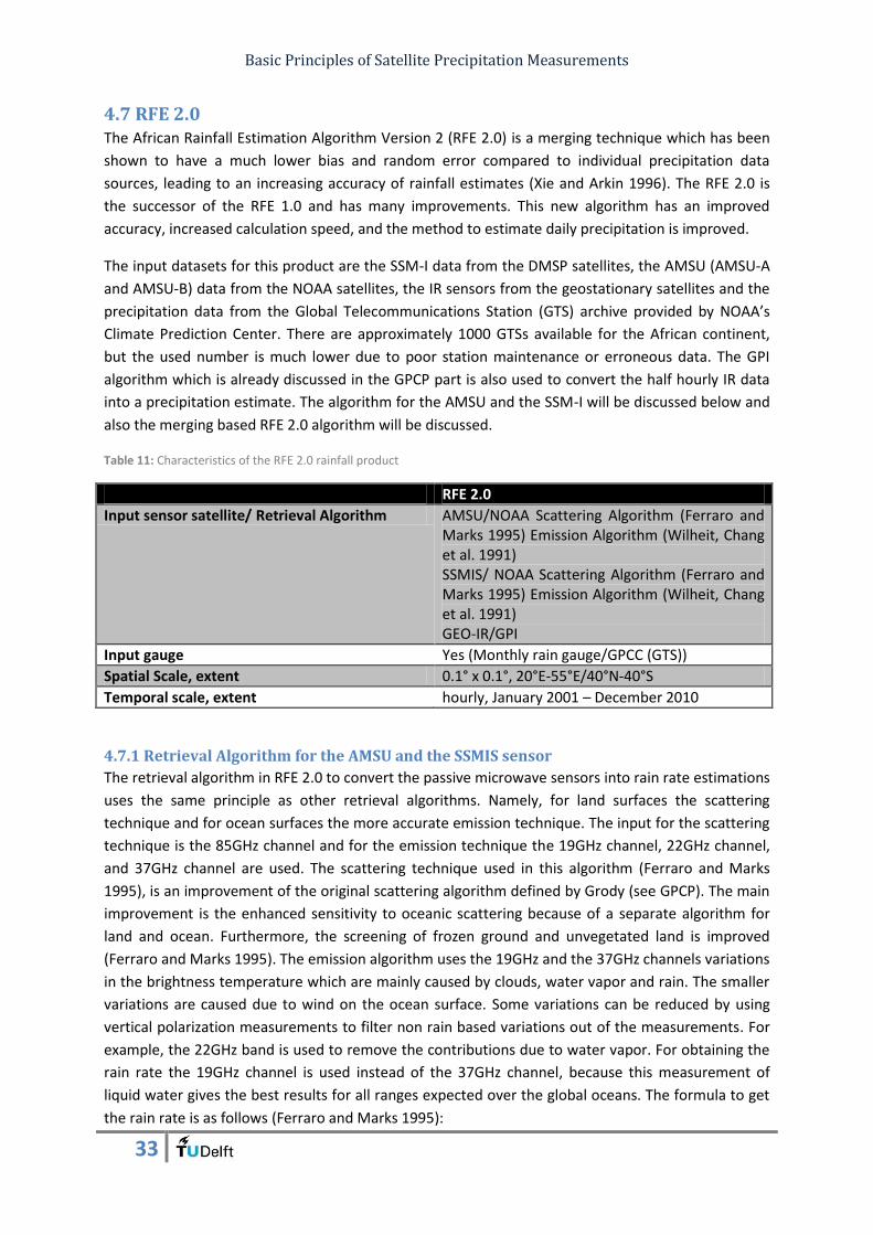
Basic Principles of Satellite Precipitation Measurements

33

4.7 RFE 2.0 The African Rainfall Estimation Algorithm Version 2 (RFE 2.0) is a merging technique which has been

shown to have a much lower bias and random error compared to individual precipitation data

sources, leading to an increasing accuracy of rainfall estimates (Xie and Arkin 1996). The RFE 2.0 is

the successor of the RFE 1.0 and has many improvements. This new algorithm has an improved

accuracy, increased calculation speed, and the method to estimate daily precipitation is improved.

The input datasets for this product are the SSM-I data from the DMSP satellites, the AMSU (AMSU-A

and AMSU-B) data from the NOAA satellites, the IR sensors from the geostationary satellites and the

precipitation data from the Global Telecommunications Station (GTS) archive provided by NOAA’s

Climate Prediction Center. There are approximately 1000 GTSs available for the African continent,

but the used number is much lower due to poor station maintenance or erroneous data. The GPI

algorithm which is already discussed in the GPCP part is also used to convert the half hourly IR data

into a precipitation estimate. The algorithm for the AMSU and the SSM-I will be discussed below and

also the merging based RFE 2.0 algorithm will be discussed.

Table 11: Characteristics of the RFE 2.0 rainfall product

RFE 2.0

Input sensor satellite/ Retrieval Algorithm AMSU/NOAA Scattering Algorithm (Ferraro and Marks 1995) Emission Algorithm (Wilheit, Chang et al. 1991) SSMIS/ NOAA Scattering Algorithm (Ferraro and Marks 1995) Emission Algorithm (Wilheit, Chang et al. 1991) GEO-IR/GPI

Input gauge Yes (Monthly rain gauge/GPCC (GTS))

Spatial Scale, extent 0.1° x 0.1°, 20°E-55°E/40°N-40°S

Temporal scale, extent hourly, January 2001 – December 2010

4.7.1 Retrieval Algorithm for the AMSU and the SSMIS sensor

The retrieval algorithm in RFE 2.0 to convert the passive microwave sensors into rain rate estimations

uses the same principle as other retrieval algorithms. Namely, for land surfaces the scattering

technique and for ocean surfaces the more accurate emission technique. The input for the scattering

technique is the 85GHz channel and for the emission technique the 19GHz channel, 22GHz channel,

and 37GHz channel are used. The scattering technique used in this algorithm (Ferraro and Marks

1995), is an improvement of the original scattering algorithm defined by Grody (see GPCP). The main

improvement is the enhanced sensitivity to oceanic scattering because of a separate algorithm for

land and ocean. Furthermore, the screening of frozen ground and unvegetated land is improved

(Ferraro and Marks 1995). The emission algorithm uses the 19GHz and the 37GHz channels variations

in the brightness temperature which are mainly caused by clouds, water vapor and rain. The smaller

variations are caused due to wind on the ocean surface. Some variations can be reduced by using

vertical polarization measurements to filter non rain based variations out of the measurements. For

example, the 22GHz band is used to remove the contributions due to water vapor. For obtaining the

rain rate the 19GHz channel is used instead of the 37GHz channel, because this measurement of

liquid water gives the best results for all ranges expected over the global oceans. The formula to get

the rain rate is as follows (Ferraro and Marks 1995):

Basic Principles of Satellite Precipitation Measurements

34

The AMSU-B rainfall retrieval is very similar as the one used for the SSM-I instruments.

4.7.2 Two step merging process

The next step is merging the data sources. This is needed to get a complete spatial coverage and

lowers the random errors. The merging process consists of two steps. The first step is to reduce the

random errors of all the satellites sources. This is done by combining GPI, SSM-I and AMSU data

linearly through a maximum likelihood estimation method to determine the weighting coefficient.

The weighting equation is the following:

In which Wi is the weighting coefficient for source i, σi2 the random error for source i. The random

error is defined for each grid and each source monthly. So when the random error is smaller (better

accuracy) the weighting coefficient of that source is higher.

Over land areas, the GPCC precipitation analysis is used as a standard references. To calculate the

errors, the mean difference between the monthly rainfall estimation obtained from a certain sensor

(source field) and the monthly GPCC rainfall estimation is calculated for a 7x7 array centered on the

target grid. This array is subtracted from the source field so the modified source field is created. This

is done for each grid. For the target cell the monthly random error for each individual source is

defined as the root-mean difference between the modified source field and the GPCC analysis

calculated on the same 7x7 array. Near the coast the 7x7 array is not completely filled by the GPCC

analysis, for those areas only the subset for which the values are available are used.

Over oceanic areas, the GPCC analysis is not available. In those areas the atoll gauge precipitation

observations of Morrissey and Greene (1991) are used (Xie and Arkin 1996) instead of the GPCC

rainfall estimations to calculate the random errors.

Now the weighting coefficients are determined, the rainfall estimates from the different sources (Si)

are combined to calculate the precipitation estimate (S) which will have a reduced random error. The

following equation is used:

The second step in the merging process is to compare this satellite precipitation estimate with the

GPCC rain gauge data set to remove the bias as much as possible. The precipitation will maintain the

shape of the combined satellite precipitation estimates, while the magnitude is inferred from the

GPCC dataset. For location within the direct surrounding of a GPCC rain gauge gets the magnitude of

precipitation as measured with the GPCC rain station. When the distance from the stations increases,

the rainfall estimates rely more on the combined satellite precipitation estimate (NOAA 2001).

In Figure 15 the flow chart of the RFE 2.0 is shown.

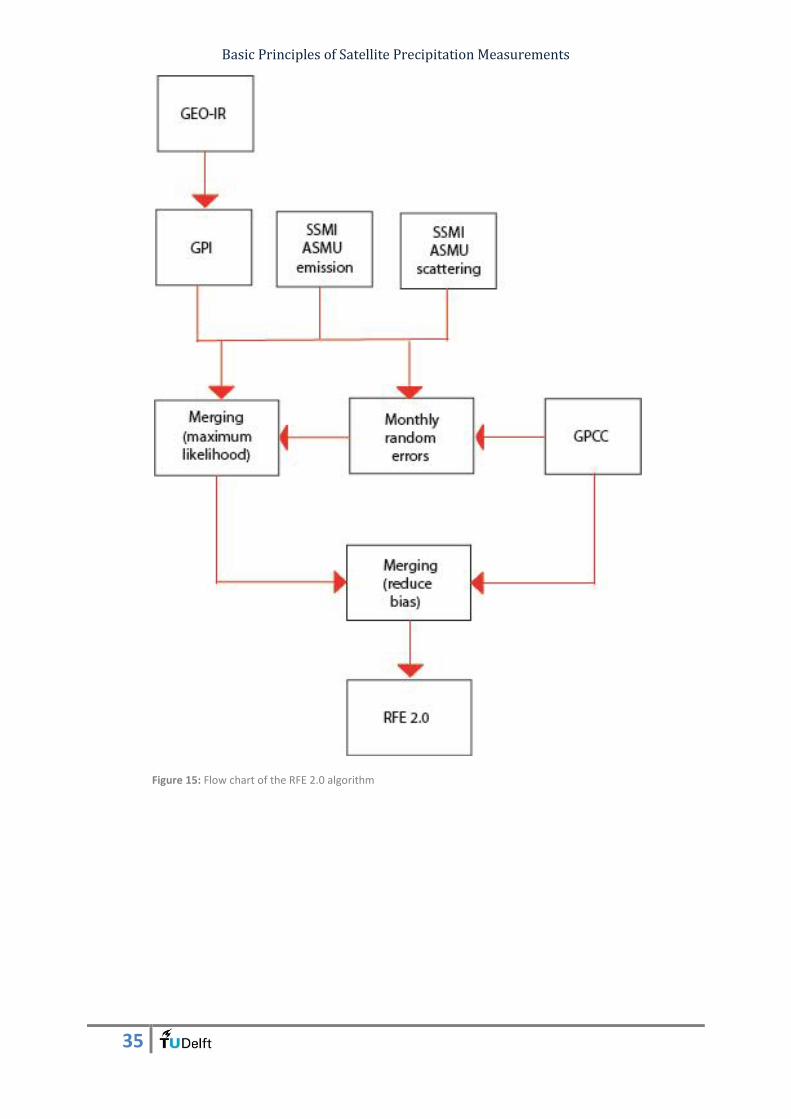
Basic Principles of Satellite Precipitation Measurements

35

Figure 15: Flow chart of the RFE 2.0 algorithm

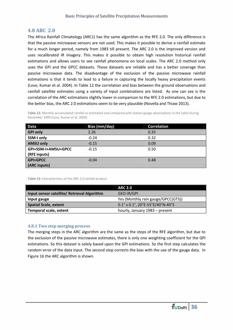
Basic Principles of Satellite Precipitation Measurements

36

4.8 ARC 2.0 The Africa Rainfall Climatology (ARC1) has the same algorithm as the RFE 2.0. The only difference is

that the passive microwave sensors are not used. This makes it possible to derive a rainfall estimate

for a much longer period, namely from 1983 till present. The ARC 2.0 is the improved version and

uses recalibrated IR imagery. This makes it possible to obtain high resolution historical rainfall

estimations and allows users to see rainfall phenomena on local scales. The ARC 2.0 method only

uses the GPI and the GPCC datasets. Those datasets are reliable and has a better coverage than

passive microwave data. The disadvantage of the exclusion of the passive microwave rainfall

estimations is that it tends to lead to a failure in capturing the locally heavy precipitation events

(Love, Kumar et al. 2004). In Table 12 the correlation and bias between the ground observations and

rainfall satellite estimates using a variety of input combinations are listed. As one can see is the

correlation of the ARC estimations slightly lower in comparison to the RFE 2.0 estimations, but due to

the better bias, the ARC 2.0 estimations seem to be very plausible (Novella and Thiaw 2013).

Table 13: Characteristics of the ARC 2.0 rainfall product

ARC 2.0

Input sensor satellite/ Retrieval Algorithm GEO-IR/GPI

Input gauge Yes (Monthly rain gauge/GPCC(GTS))

Spatial Scale, extent 0.1° x 0.1°, 20°E-55°E/40°N-40°S

Temporal scale, extent hourly, January 1983 – present

4.8.1 Two step merging process

The merging steps in the ARC algorithm are the same as the steps of the RFE algorithm, but due to

the exclusion of the passive microwave estimates, there is only one weighting coefficient for the GPI

estimations. So this dataset is solely based upon the GPI estimations. So the first step calculates the

random error of the data input. The second step corrects the bias with the use of the gauge data. In

Figure 16 the ARC algorithm is shown.

Table 12: Monthly accumulated rainfall as estimated and compared with station gauge observations in the Sahel during December 1999 (Love, Kumar et al. 2004)

Data Bias (mm/day) Correlation

GPI only 2.26 0.35

SSM-I only -0.24 0.32

AMSU only -0.15 0.09

GPI+SSM-I+AMSU+GPCC (RFE inputs)

-0.15 0.50

GPI+GPCC (ARC inputs)

-0.04 0.48

Basic Principles of Satellite Precipitation Measurements

37

Figure 16: Flow chart of the ARC 2.0 algorithm

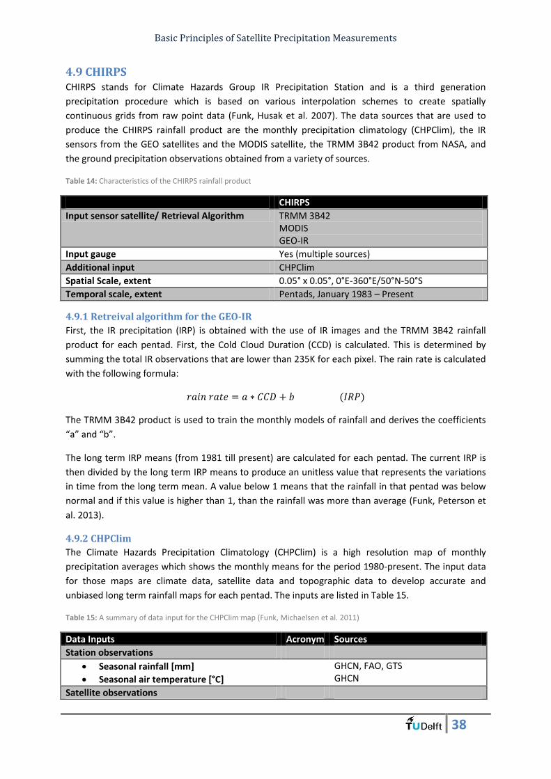
Basic Principles of Satellite Precipitation Measurements

38

4.9 CHIRPS CHIRPS stands for Climate Hazards Group IR Precipitation Station and is a third generation

precipitation procedure which is based on various interpolation schemes to create spatially

continuous grids from raw point data (Funk, Husak et al. 2007). The data sources that are used to

produce the CHIRPS rainfall product are the monthly precipitation climatology (CHPClim), the IR

sensors from the GEO satellites and the MODIS satellite, the TRMM 3B42 product from NASA, and

the ground precipitation observations obtained from a variety of sources.

Table 14: Characteristics of the CHIRPS rainfall product

CHIRPS

Input sensor satellite/ Retrieval Algorithm TRMM 3B42 MODIS GEO-IR

Input gauge Yes (multiple sources)

Additional input CHPClim

Spatial Scale, extent 0.05° x 0.05°, 0°E-360°E/50°N-50°S

Temporal scale, extent Pentads, January 1983 – Present

4.9.1 Retreival algorithm for the GEO-IR

First, the IR precipitation (IRP) is obtained with the use of IR images and the TRMM 3B42 rainfall

product for each pentad. First, the Cold Cloud Duration (CCD) is calculated. This is determined by

summing the total IR observations that are lower than 235K for each pixel. The rain rate is calculated

with the following formula:

The TRMM 3B42 product is used to train the monthly models of rainfall and derives the coefficients

“a” and “b”.

The long term IRP means (from 1981 till present) are calculated for each pentad. The current IRP is

then divided by the long term IRP means to produce an unitless value that represents the variations

in time from the long term mean. A value below 1 means that the rainfall in that pentad was below

normal and if this value is higher than 1, than the rainfall was more than average (Funk, Peterson et

al. 2013).

4.9.2 CHPClim

The Climate Hazards Precipitation Climatology (CHPClim) is a high resolution map of monthly

precipitation averages which shows the monthly means for the period 1980-present. The input data

for those maps are climate data, satellite data and topographic data to develop accurate and

unbiased long term rainfall maps for each pentad. The inputs are listed in Table 15.

Table 15: A summary of data input for the CHPClim map (Funk, Michaelsen et al. 2011)

Data Inputs Acronym Sources

Station observations

Seasonal rainfall [mm]

Seasonal air temperature [°C]

GHCN, FAO, GTS GHCN

Satellite observations

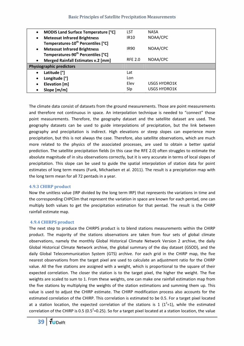
Basic Principles of Satellite Precipitation Measurements

39

MODIS Land Surface Temperature [°C]

Meteosat Infrared Brightness Temperatures-10th Percentiles [°C]

Meteosat Infrared Brightness Temperatures-90th Percentiles [°C]

Merged Rainfall Estimates v.2 [mm]

LST IR10 IR90 RFE 2.0

NASA NOAA/CPC NOAA/CPC NOAA/CPC

Physiographic predictors

Latitude [°]

Longitude [°]

Elevation [m]

Slope [m/m]

Lat Lon Elev Slp

USGS HYDRO1K USGS HYDRO1K

The climate data consist of datasets from the ground measurements. Those are point measurements

and therefore not continuous in space. An interpolation technique is needed to “connect” those

point measurements. Therefore, the geography dataset and the satellite dataset are used. The

geography datasets can be used to guide interpolations of precipitation, but the link between

geography and precipitation is indirect. High elevations or steep slopes can experience more

precipitation, but this is not always the case. Therefore, also satellite observations, which are much

more related to the physics of the associated processes, are used to obtain a better spatial

prediction. The satellite precipitation fields (in this case the RFE 2.0) often struggles to estimate the

absolute magnitude of in situ observations correctly, but it is very accurate in terms of local slopes of

precipitation. This slope can be used to guide the spatial interpolation of station data for point

estimates of long term means (Funk, Michaelsen et al. 2011). The result is a precipitation map with

the long term mean for all 72 pentads in a year.

4.9.3 CHIRP product

Now the unitless value (IRP divided by the long term IRP) that represents the variations in time and

the corresponding CHPClim that represent the variation in space are known for each pentad, one can

multiply both values to get the precipitation estimation for that pentad. The result is the CHIRP

rainfall estimate map.

4.9.4 CHIRPS product

The next step to produce the CHIRPS product is to blend stations measurements within the CHIRP

product. The majority of the stations observations are taken from four sets of global climate

observations, namely the monthly Global Historical Climate Network Version 2 archive, the daily

Global Historical Climate Network archive, the global summary of the day dataset (GSOD), and the

daily Global Telecommunication System (GTS) archive. For each grid in the CHIRP map, the five

nearest observations from the target pixel are used to calculate an adjustment ratio for the CHIRP

value. All the five stations are assigned with a weight, which is proportional to the square of their

expected correlation. The closer the station is to the target pixel, the higher the weight. The five

weights are scaled to sum to 1. From these weights, one can make one rainfall estimation map from

the five stations by multiplying the weights of the station estimations and summing them up. This

value is used to adjust the CHIRP estimate. The CHIRP modification process also accounts for the

estimated correlation of the CHIRP. This correlation is estimated to be 0.5. For a target pixel located

at a station location, the expected correlation of the stations is 1 (12=1), while the estimated

correlation of the CHIRP is 0.5 (0.52=0.25). So for a target pixel located at a station location, the value

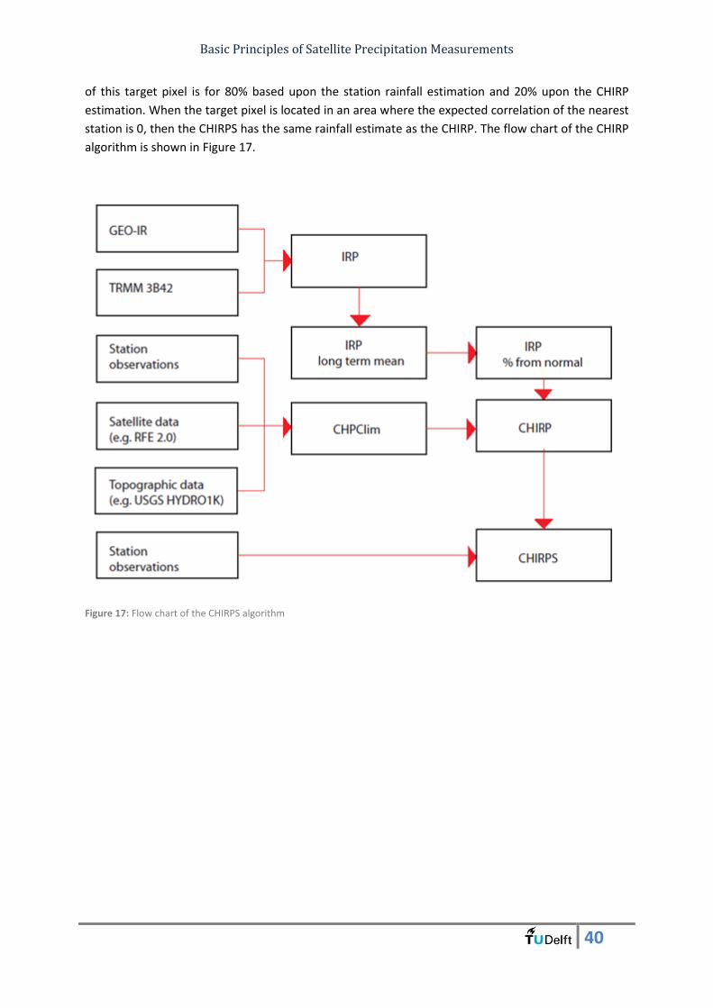
Basic Principles of Satellite Precipitation Measurements

40

of this target pixel is for 80% based upon the station rainfall estimation and 20% upon the CHIRP

estimation. When the target pixel is located in an area where the expected correlation of the nearest

station is 0, then the CHIRPS has the same rainfall estimate as the CHIRP. The flow chart of the CHIRP

algorithm is shown in Figure 17.

Figure 17: Flow chart of the CHIRPS algorithm

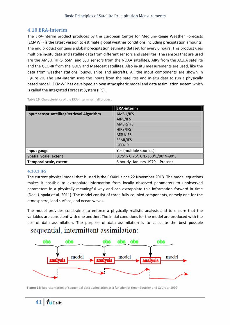
Basic Principles of Satellite Precipitation Measurements

41

4.10 ERA-interim The ERA-interim product produces by the European Centre for Medium-Range Weather Forecasts

(ECMWF) is the latest version to estimate global weather conditions including precipitation amounts.

The end product contains a global precipitation estimate dataset for every 6 hours. This product uses

multiple in-situ data and satellite data from different sensors and satellites. The sensors that are used

are the AMSU, HIRS, SSMI and SSU sensors from the NOAA satellites, AIRS from the AQUA satellite

and the GEO-IR from the GOES and Meteosat satellites. Also in-situ measurements are used, like the

data from weather stations, buoys, ships and aircrafts. All the input components are shown in

Figure 20. The ERA-interim uses the inputs from the satellites and in-situ data to run a physically

based model. ECMWF has developed an own atmospheric model and data assimilation system which

is called the Integrated Forecast System (IFS).

4.10.1 IFS

The current physical model that is used is the CY40r1 since 22 November 2013. The model equations

makes it possible to extrapolate information from locally observed parameters to unobserved

parameters in a physically meaningful way and can extrapolate this information forward in time

(Dee, Uppala et al. 2011). The model consist of three fully coupled components, namely one for the

atmosphere, land surface, and ocean waves.

The model provides constraints to enforce a physically realistic analysis and to ensure that the

variables are consistent with one another. The initial conditions for the model are produced with the

use of data assimilation. The purpose of data assimilation is to calculate the best possible

Table 16: Characteristics of the ERA-interim rainfall product

ERA-interim

Input sensor satellite/Retrieval Algorithm AMSU/IFS AIRS/IFS AMSR/IFS HIRS/IFS MSU/IFS SSMI/IFS GEO-IR

Input gauge Yes (multiple sources)

Spatial Scale, extent 0.75° x 0.75°, 0°E-360°E/90°N-90°S

Temporal scale, extent 6 hourly, January 1979 – Present

Figure 18: Representation of sequential data assimilation as a function of time (Bouttier and Courtier 1999)

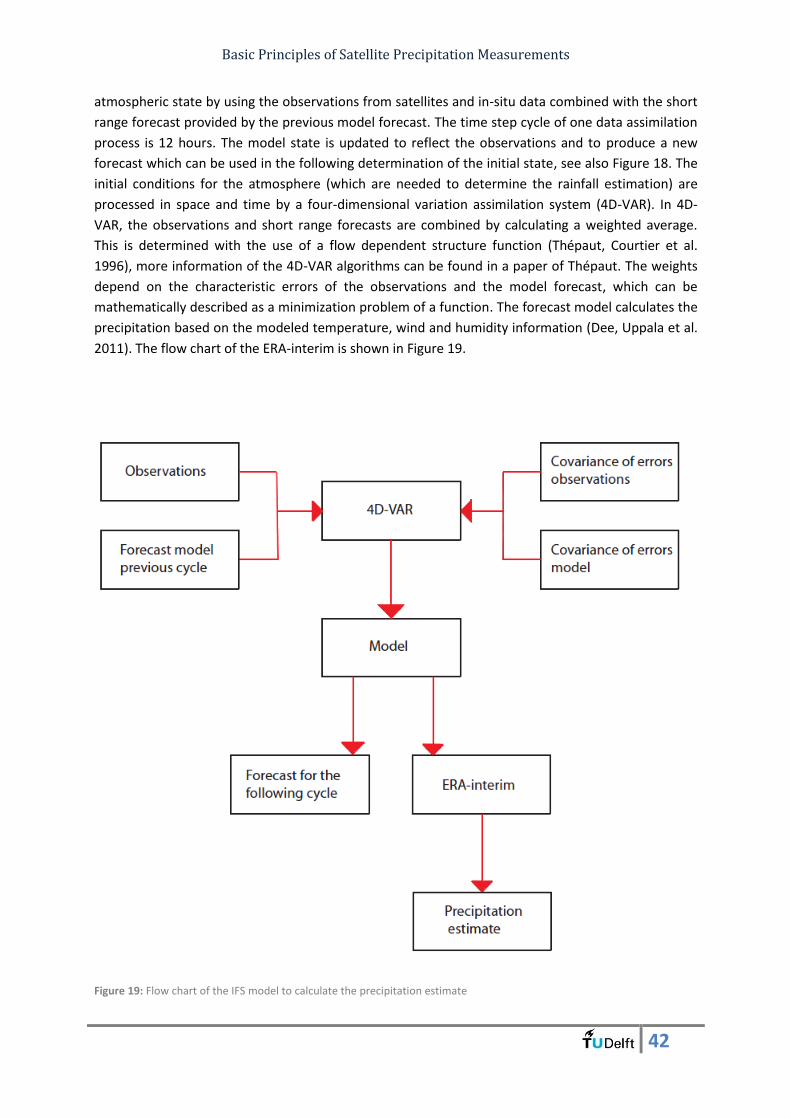
Basic Principles of Satellite Precipitation Measurements

42

atmospheric state by using the observations from satellites and in-situ data combined with the short

range forecast provided by the previous model forecast. The time step cycle of one data assimilation

process is 12 hours. The model state is updated to reflect the observations and to produce a new

forecast which can be used in the following determination of the initial state, see also Figure 18. The

initial conditions for the atmosphere (which are needed to determine the rainfall estimation) are

processed in space and time by a four-dimensional variation assimilation system (4D-VAR). In 4D-

VAR, the observations and short range forecasts are combined by calculating a weighted average.

This is determined with the use of a flow dependent structure function (Thépaut, Courtier et al.

1996), more information of the 4D-VAR algorithms can be found in a paper of Thépaut. The weights

depend on the characteristic errors of the observations and the model forecast, which can be

mathematically described as a minimization problem of a function. The forecast model calculates the

precipitation based on the modeled temperature, wind and humidity information (Dee, Uppala et al.

2011). The flow chart of the ERA-interim is shown in Figure 19.

Figure 19: Flow chart of the IFS model to calculate the precipitation estimate

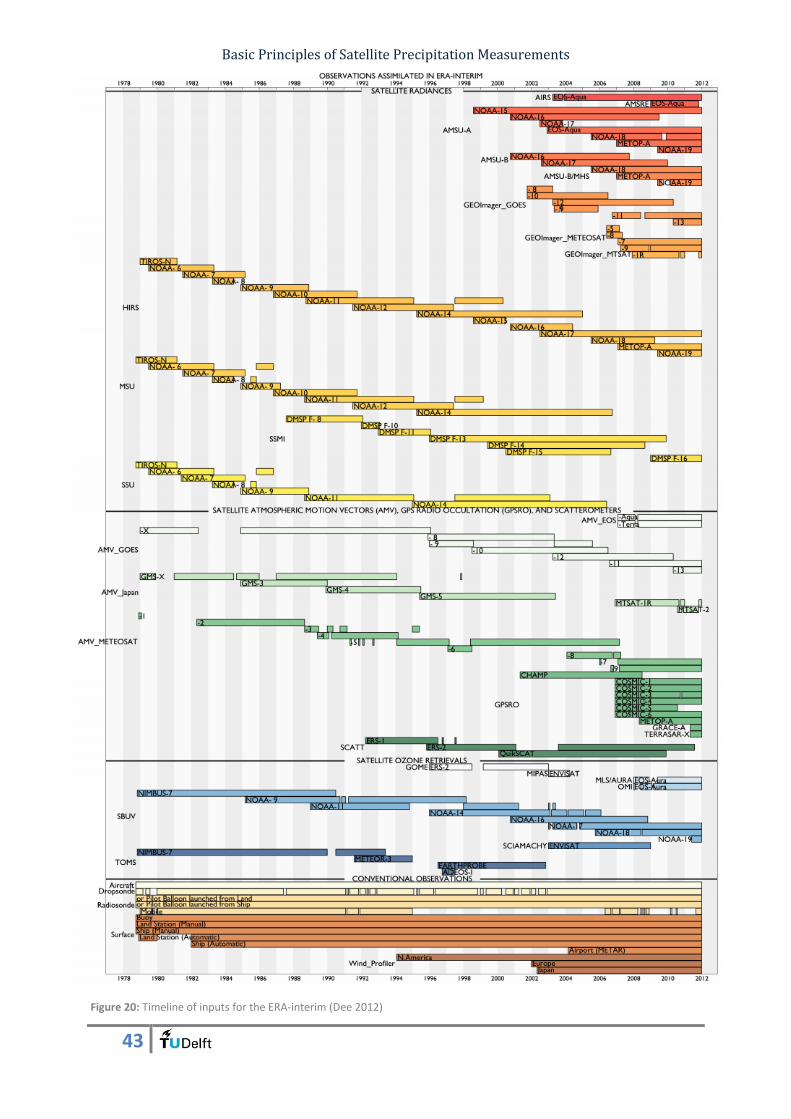
Basic Principles of Satellite Precipitation Measurements

43

Figure 20: Timeline of inputs for the ERA-interim (Dee 2012)

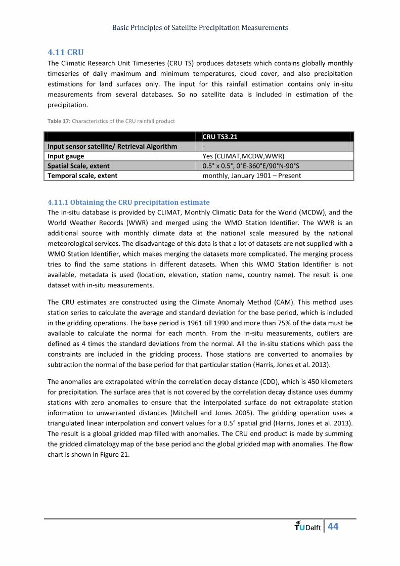
Basic Principles of Satellite Precipitation Measurements

44

4.11 CRU The Climatic Research Unit Timeseries (CRU TS) produces datasets which contains globally monthly

timeseries of daily maximum and minimum temperatures, cloud cover, and also precipitation

estimations for land surfaces only. The input for this rainfall estimation contains only in-situ

measurements from several databases. So no satellite data is included in estimation of the

precipitation.

4.11.1 Obtaining the CRU precipitation estimate

The in-situ database is provided by CLIMAT, Monthly Climatic Data for the World (MCDW), and the

World Weather Records (WWR) and merged using the WMO Station Identifier. The WWR is an

additional source with monthly climate data at the national scale measured by the national

meteorological services. The disadvantage of this data is that a lot of datasets are not supplied with a

WMO Station Identifier, which makes merging the datasets more complicated. The merging process

tries to find the same stations in different datasets. When this WMO Station Identifier is not

available, metadata is used (location, elevation, station name, country name). The result is one

dataset with in-situ measurements.

The CRU estimates are constructed using the Climate Anomaly Method (CAM). This method uses

station series to calculate the average and standard deviation for the base period, which is included

in the gridding operations. The base period is 1961 till 1990 and more than 75% of the data must be

available to calculate the normal for each month. From the in-situ measurements, outliers are

defined as 4 times the standard deviations from the normal. All the in-situ stations which pass the

constraints are included in the gridding process. Those stations are converted to anomalies by

subtraction the normal of the base period for that particular station (Harris, Jones et al. 2013).

The anomalies are extrapolated within the correlation decay distance (CDD), which is 450 kilometers

for precipitation. The surface area that is not covered by the correlation decay distance uses dummy

stations with zero anomalies to ensure that the interpolated surface do not extrapolate station

information to unwarranted distances (Mitchell and Jones 2005). The gridding operation uses a

triangulated linear interpolation and convert values for a 0.5° spatial grid (Harris, Jones et al. 2013).

The result is a global gridded map filled with anomalies. The CRU end product is made by summing

the gridded climatology map of the base period and the global gridded map with anomalies. The flow

chart is shown in Figure 21.

Table 17: Characteristics of the CRU rainfall product

CRU TS3.21

Input sensor satellite/ Retrieval Algorithm -

Input gauge Yes (CLIMAT,MCDW,WWR)

Spatial Scale, extent 0.5° x 0.5°, 0°E-360°E/90°N-90°S

Temporal scale, extent monthly, January 1901 – Present

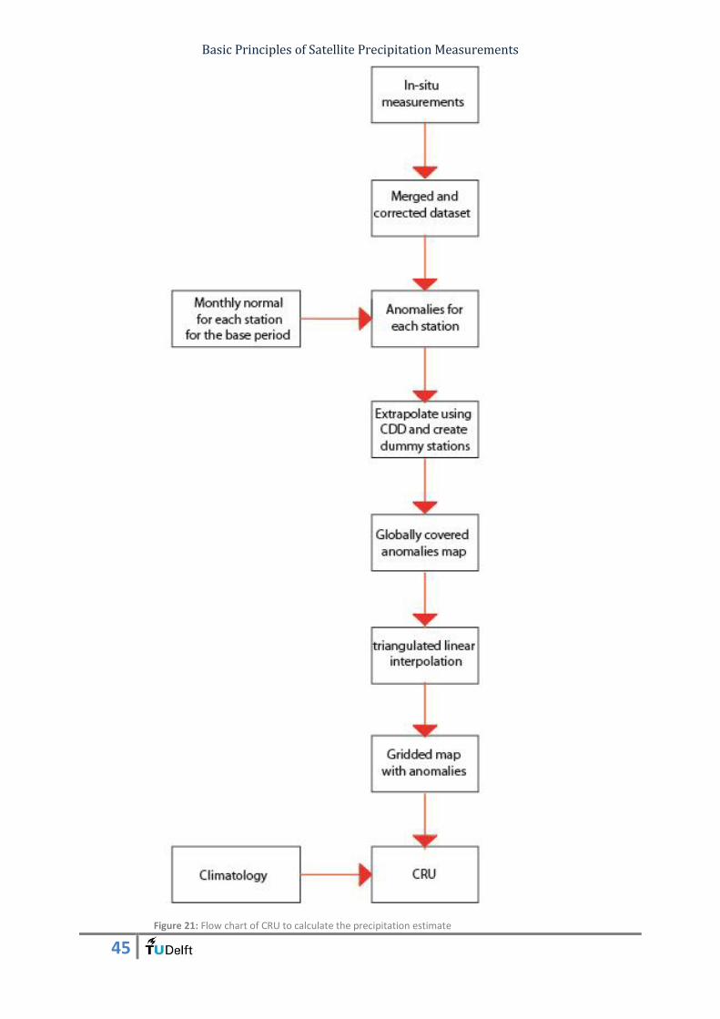
Basic Principles of Satellite Precipitation Measurements

45

Figure 21: Flow chart of CRU to calculate the precipitation estimate

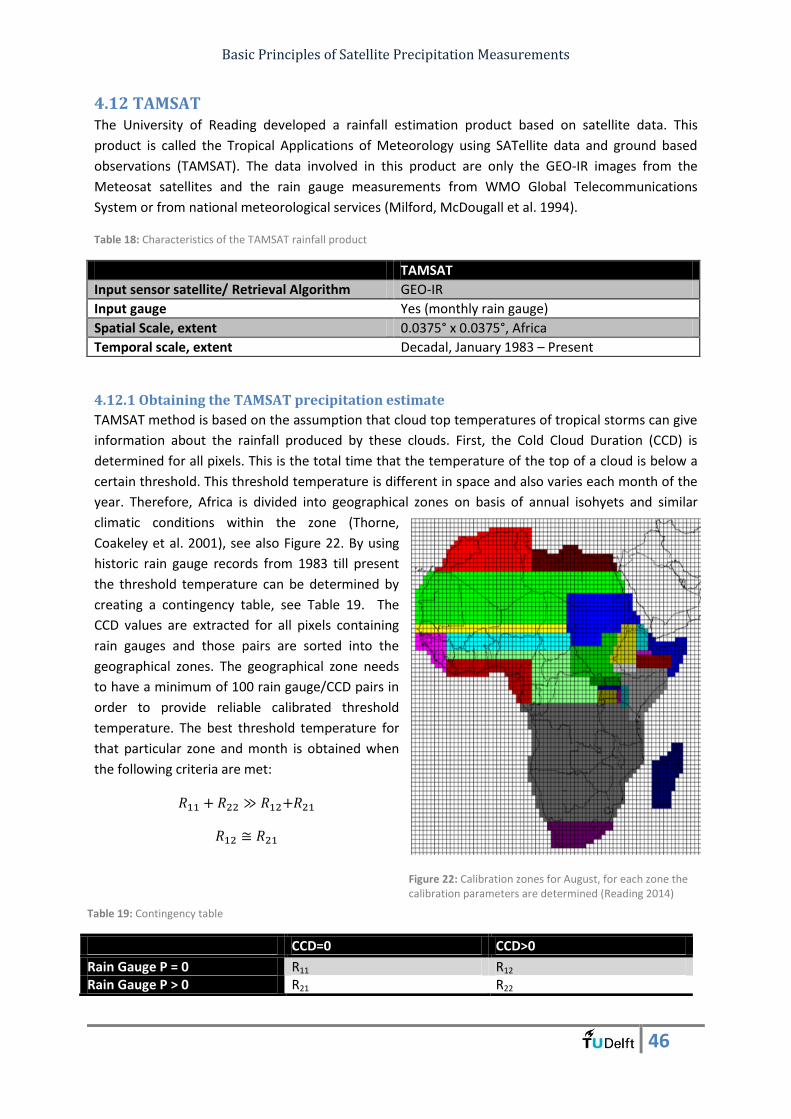
Basic Principles of Satellite Precipitation Measurements

46

4.12 TAMSAT The University of Reading developed a rainfall estimation product based on satellite data. This

product is called the Tropical Applications of Meteorology using SATellite data and ground based

observations (TAMSAT). The data involved in this product are only the GEO-IR images from the

Meteosat satellites and the rain gauge measurements from WMO Global Telecommunications

System or from national meteorological services (Milford, McDougall et al. 1994).

4.12.1 Obtaining the TAMSAT precipitation estimate

TAMSAT method is based on the assumption that cloud top temperatures of tropical storms can give

information about the rainfall produced by these clouds. First, the Cold Cloud Duration (CCD) is

determined for all pixels. This is the total time that the temperature of the top of a cloud is below a

certain threshold. This threshold temperature is different in space and also varies each month of the

year. Therefore, Africa is divided into geographical zones on basis of annual isohyets and similar

climatic conditions within the zone (Thorne,

Coakeley et al. 2001), see also Figure 22. By using

historic rain gauge records from 1983 till present

the threshold temperature can be determined by

creating a contingency table, see Table 19. The

CCD values are extracted for all pixels containing

rain gauges and those pairs are sorted into the

geographical zones. The geographical zone needs

to have a minimum of 100 rain gauge/CCD pairs in

order to provide reliable calibrated threshold

temperature. The best threshold temperature for

that particular zone and month is obtained when

the following criteria are met:

Table 18: Characteristics of the TAMSAT rainfall product

TAMSAT

Input sensor satellite/ Retrieval Algorithm GEO-IR

Input gauge Yes (monthly rain gauge)

Spatial Scale, extent 0.0375° x 0.0375°, Africa

Temporal scale, extent Decadal, January 1983 – Present

Figure 22: Calibration zones for August, for each zone the calibration parameters are determined (Reading 2014)

Table 19: Contingency table

CCD=0 CCD>0

Rain Gauge P = 0 R11 R12

Rain Gauge P > 0 R21 R22

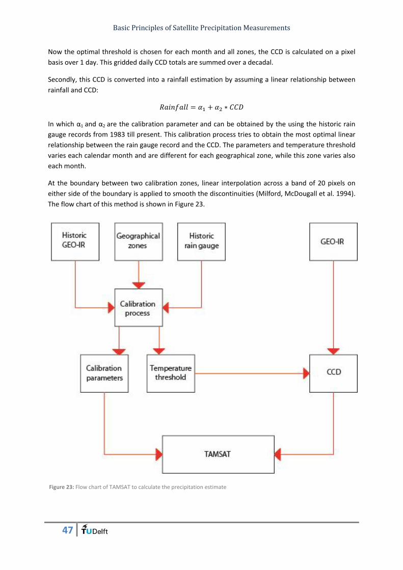
Basic Principles of Satellite Precipitation Measurements

47

Now the optimal threshold is chosen for each month and all zones, the CCD is calculated on a pixel

basis over 1 day. This gridded daily CCD totals are summed over a decadal.

Secondly, this CCD is converted into a rainfall estimation by assuming a linear relationship between

rainfall and CCD:

In which α1 and α2 are the calibration parameter and can be obtained by the using the historic rain

gauge records from 1983 till present. This calibration process tries to obtain the most optimal linear

relationship between the rain gauge record and the CCD. The parameters and temperature threshold

varies each calendar month and are different for each geographical zone, while this zone varies also

each month.

At the boundary between two calibration zones, linear interpolation across a band of 20 pixels on

either side of the boundary is applied to smooth the discontinuities (Milford, McDougall et al. 1994).

The flow chart of this method is shown in Figure 23.

Figure 23: Flow chart of TAMSAT to calculate the precipitation estimate

Basic Principles of Satellite Precipitation Measurements

48

5. Concluding tables In this chapter some table are shown which give some additional insight in the techniques and

sensors that are used to obtain the precipitation estimation of a product. All the information in this

chapter is already discussed in the previous chapters, therefore only some tables will be shown

without any explanation. The techniques are shown in Table 20 and in Table 21 the used sensors are

for each precipitation estimates are shown. In Figure 24 All the algorithms are visualized with flow

charts.

Table 20: The precipitation products and the used techniques to obtain that estimation

Techniques TRM

M

CM

OR

PH

GP

CP

GP

CP

1D

D

PER

SIAN

N

GSM

aP

RFE 2

.0

AR

C 2

.0

CH

IRP

S

ERA

-

inte

rim

CR

U

TAM

SAT

GEO IR for GPI, AGPI or TMPI x x x x x

GEO IR for motion vector x x

GEO IR for Cold Cloud Duration x x

GEO IR for VAR algorithm x x

GEO IR for Artificial Neural Network x

Precipitation Radar x x x

TRMM 2A12 ( TMI only) x

TRMM 2B31 (TMI and PR) x x

GPROF x x

LEO ( emission and scattering technique) x x x x x

Rain Gauge measurements x x x x x x x x x

All kinds of satellite observations as input for a model

x

Table 21: The used sensors to obtain the precipitation estimation

Sensors TRM

M

3B

43

CM

OR

PH

GP

CP

GP

CP

1D

D

PER

SIAN

N

GSM

aP

RFE 2

.0

AR

C 2

.0

CH

IRP

S

ERA

-in

terim

CR

U

TAM

SAT

GEO

SEVIRI

LEO

x

x

x

x

x

x

x

x

x

x

x

Precipitation Radar x

AMSU x x x x x

SSMI x x x x x x x

TMI x x x x x

AMSR

x x x x

Rainfall Measurements

Ground Measurements

x

x

x

x

x

x

x

x

x

Rainfall Products

TRMM 3B42 x

RFE 2.0 x

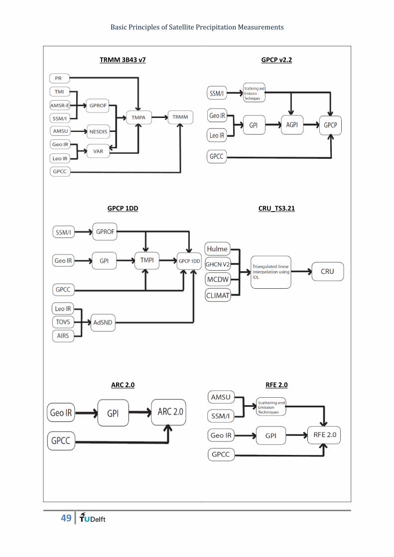
Basic Principles of Satellite Precipitation Measurements

49

TRMM 3B43 v7

GPCP v2.2

GPCP 1DD

CRU_TS3.21

ARC 2.0

RFE 2.0

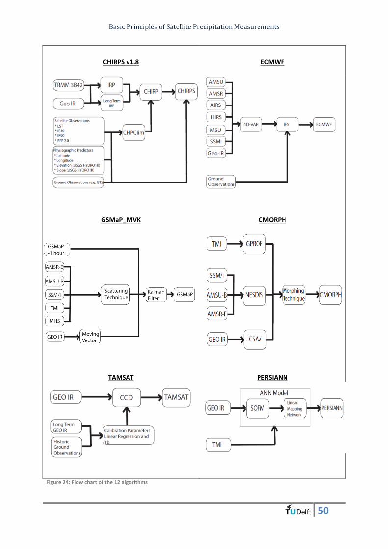
Basic Principles of Satellite Precipitation Measurements

50

CHIRPS v1.8

ECMWF

GSMaP_MVK

CMORPH

TAMSAT PERSIANN

Figure 24: Flow chart of the 12 algorithms

Basic Principles of Satellite Precipitation Measurements

51

6. References Adler, R. F., et al. (2003). "The version-2 Global Precipitation Climatology Project (GPCP) monthly precipitation analysis (1979–present)." Journal of Hydrometeorology 4(6). Aonashi, K., et al. (1996). "An over-ocean precipitation retrieval using SSM/I multichannel brightness temperatures." Journal of the Meteorological Society of Japan 74(5): 617-637. Arkin, P. A. and B. N. Meisner (1987). "The relationship between large-scale convective rainfall and cold cloud over the western hemisphere during 1982-84." Monthly Weather Review 115(1): 51-74. Bouttier, F. and P. Courtier (1999). "Data assimilation concept and methods." Meteorological Training Course Lecture Series. Brown, J. E. (2006). "An analysis of the performance of hybrid infrared and microwave satellite precipitation algorithms over India and adjacent regions." Remote sensing of environment 101(1): 63-81. Dee, D. (2012). Observations Assimilated in ERA-interim. ECMWF, ECMWF. Dee, D., et al. (2011). "The ERA‐Interim reanalysis: Configuration and performance of the data assimilation system." Quarterly Journal of the Royal Meteorological Society 137(656): 553-597. Ferraro, R. R. and G. F. Marks (1995). "The development of SSM/I rain-rate retrieval algorithms using ground-based radar measurements." Journal of Atmospheric and Oceanic Technology 12(4): 755-770. Funk, C., et al. (2007). "Third generation rainfall climatologies: satellite rainfall and topography provide a basis for smart interpolation." Funk, C., et al. (2011). "Mapping recent decadal climate variations in precipitation and temperature across Eastern Africa and the Sahel." Funk, C., et al. (2013). "A Quasi-Global Precipitation Time Series for Drought Monitoring." USGS. GOES (2014). "GOES." Retrieved 9 May, 2014, from http://www.goes-r.gov/mission/history.html. Grody, N. C. (1991). "Classification of snow cover and precipitation using the Special Sensor Microwave Imager." Journal of Geophysical Research: Atmospheres (1984–2012) 96(D4): 7423-7435. Grossberg, S. (1969). "Embedding fields: A theory of learning with physiological implications." Journal of Mathematical Psychology 6(2): 209-239. Harris, I., et al. (2013). "Updated high‐resolution grids of monthly climatic observations–the CRU TS3. 10 Dataset." International Journal of Climatology. Hsu, K.-l., et al. (1997). "Precipitation estimation from remotely sensed information using artificial neural networks." Journal of Applied Meteorology 36(9): 1176-1190. Huffman, G. J., et al. (1997). "The global precipitation climatology project (GPCP) combined precipitation dataset." Bulletin of the American Meteorological Society 78(1): 5-20. Huffman, G. J., et al. (2007). "The TRMM Multisatellite Precipitation Analysis (TMPA): Quasi-global, multiyear, combined-sensor precipitation estimates at fine scales." Journal of Hydrometeorology 8(1). Huffman, G. J., et al. (2010). The TRMM multi-satellite precipitation analysis (TMPA). Satellite rainfall applications for surface hydrology, Springer: 3-22. Huffman, G. J., et al. (2001). "Global precipitation at one-degree daily resolution from multisatellite observations." Journal of Hydrometeorology 2(1): 36-50. Huffman, G. J. and D. Bolvin (2013). "GPCP Version 2.2 SG Combined Precipitation Data Set Documentation." NASA Goddard Space Flight Center, Mesoscale Atmospheric PRocsses Laboratory and Science Systems and Applications, Inc.

Basic Principles of Satellite Precipitation Measurements

52

Huffman, G. J. and D. Bolvin (2013). "Version 1.2 GPCP One-Degree Daily Precipitation Data Set Documentation." Mesoscale Atmosphereic Processes Laboratory. Janowiak, J. E. and P. A. Arkin (1991). "Rainfall variations in the tropics during 1986–1989, as estimated from observations of cloud‐top temperature." Journal of Geophysical Research: Oceans (1978–2012) 96(S01): 3359-3373. Joyce, R. J., et al. (2004). "CMORPH: A method that produces global precipitation estimates from passive microwave and infrared data at high spatial and temporal resolution." Journal of Hydrometeorology 5(3). Joyce, R. J., et al. (2010). CMORPH: A “Morphing” Approach for High Resolution Precipitation Product Generation. Satellite Rainfall Applications for Surface Hydrology, Springer: 23-37. Kidd, C., et al. (2009). "Satellite Precipitation Measurements for Water Resource Monitoring1." JAWRA Journal of the American Water Resources Association 45(3): 567-579. Kohonen, T. (1982). "Self-organized formation of topologically correct feature maps." Biological cybernetics 43(1): 59-69. Kubota, T., et al. (2007). "Global precipitation map using satellite-borne microwave radiometers by the GSMaP Project: Production and validation." Geoscience and Remote Sensing, IEEE Transactions on 45(7): 2259-2275. Kummerow, C. and L. Giglio (1995). "A method for combining passive microwave and infrared rainfall observations." Journal of Atmospheric and Oceanic Technology 12(1): 33-45. Kummerow, C., et al. (2001). "The evolution of the Goddard profiling algorithm (GPROF) for rainfall estimation from passive microwave sensors." Journal of Applied Meteorology 40(11). Liu, G. and J. A. Curry (1992). "Retrieval of precipitation from satellite microwave measurement using both emission and scattering." Journal of Geophysical Research: Atmospheres (1984–2012) 97(D9): 9959-9974. Love, T. B., et al. (2004). "A 20-Year Daily Africa Precipitation Climatology Using Satellite and Gauge Data." 14th Conf. on Applied Meteorology. McCollum, J. R. and R. R. Ferraro (2005). "Microwave rainfall estimation over coasts." Journal of Atmospheric & Oceanic Technology 22(5). Milford, J., et al. (1994). Rainfall estimation from cold cloud duration, experience of the TAMSAT group in West Africa. Validation Problems of Rainfall Estimation by Satellite in Intertropical Africa, Guillot B., edt., Proc. Niamey workshop. Mitchell, T. D. and P. D. Jones (2005). "An improved method of constructing a database of monthly climate observations and associated high‐resolution grids." International Journal of Climatology 25(6): 693-712. NASA (2011). TRMM instruments. trmm_sat.gif. pmm.nasa.gov, NASA. Negri, A. J., et al. (2003). "A TRMM-calibrated infrared technique for global rainfall estimation." Conference on Satellite Meteorology and Oceanography 6. NOAA (2001). "The NOAA Climate Prediction Center African Rainfall Estimation Algorithm Version 2.0." Novella, N. S. and W. M. Thiaw (2013). "African Rainfall Climatology Version 2 for Famine Early Warning Systems." Journal of Applied Meteorology & Climatology 52(3). OSCAR (2014). "List of all Satellites." Retrieved 11 May, 2014, from http://www.wmo-sat.info/oscar/satellites. Petty, G. (1994). "Physical retrievals of over-ocean rain rate from multichannel microwave imagery. Part II: Algorithm implementation." Meteorology and Atmospheric Physics 54(1-4): 101-121. Pierce, H. (2013). TRMM satellite view of rainfall with the newly energized tropical disturbance in the Bay of Bengal on November 13, 2013 at 10:15 UTC. SSAI/NASA GSFC. Reading (2014). "TAMSAT." Retrieved 17 June, 2014, from http://www.met.reading.ac.uk/~vm004202/tamsat/.

Basic Principles of Satellite Precipitation Measurements

53

Seto, S., et al. (2005). "Rain/no-rain classification methods for microwave radiometer observations over land using statistical information for brightness temperatures under no-rain conditions." Journal of Applied Meteorology 44(8). Sorooshian, S., et al. (2000). "Evaluation of PERSIANN system satellite-based estimates of tropical rainfall." Bulletin of the American Meteorological Society 81(9): 2035-2046. Spencer, R. W., et al. (1989). "Precipitation retrieval over land and ocean with the SSM/I: Identification and characteristics of the scattering signal." Journal of Atmospheric and Oceanic Technology 6(2): 254-273. Susskind, J. and J. Pfaendtner (1989). Impact of interactive physical retrievals on NWP. Report on the Joint ECMWF/EUMETSAT Workshop on the Use of Satellite Data in Operational Weather Prediction: 1989–1993. Susskind, J., et al. (1997). "Characteristics of the TOVS Pathfinder Path A dataset." Bulletin of the American Meteorological Society 78(7): 1449-1472. Thépaut, J. N., et al. (1996). "Dynamical structure functions in a four‐dimensional variational assimilation: A case study." Quarterly Journal of the Royal Meteorological Society 122(530): 535-561. Thorne, V., et al. (2001). "Comparison of TAMSAT and CPC rainfall estimates with raingauges, for southern Africa." International Journal of Remote Sensing 22(10): 1951-1974. Ushio, T. and M. Kachi (2010). Kalman filtering applications for global satellite mapping of precipitation (GSMaP). Satellite Rainfall Applications for Surface Hydrology, Springer: 105-123. Ushio, T., et al. (2009). "A Kalman filter approach to the Global Satellite Mapping of Precipitation (GSMaP) from combined passive microwave and infrared radiometric data." Journal of the Meteorological Society of Japan 87: 137-151. Weng, F., et al. (2003). "Advanced microwave sounding unit cloud and precipitation algorithms." Radio Science 38(4). Wilheit, T. T., et al. (1991). "Retrieval of monthly rainfall indices from microwave radiometric measurements using probability distribution functions." Journal of Atmospheric and Oceanic Technology 8(1): 118-136. Xie, P. and P. A. Arkin (1996). "Analyses of global monthly precipitation using gauge observations, satellite estimates, and numerical model predictions." Journal of climate 9(4): 840-858. Xu, L., et al. (1999). "A microwave infrared threshold technique to improve the GOES precipitation index." Journal of Applied Meteorology 38(5): 569-579. Zhao, L. and F. Weng (2002). "Retrieval of ice cloud parameters using the Advanced Microwave Sounding Unit." Journal of Applied Meteorology 41(4).

Triple Collocation Theory and application for the Nile Basin

TU Delft Tim M. Hessels Supervisor: Prof. Dr. Wim G.M.Bastiaanssen

Triple Collocation: Theory and application for the Nile Basin

1

Triple Collocation: Theory and application for the Nile Basin

2

Table of Contents Table of Contents .................................................................................................................................... 2

1. Introduction ......................................................................................................................................... 4

2. Method ................................................................................................................................................ 6

3. Criteria for the method ....................................................................................................................... 8

3.1. Criteria 1 ....................................................................................................................................... 8

3.2. Criteria 2 ....................................................................................................................................... 8

3.3. Criteria 3 ....................................................................................................................................... 9

3.4. Criteria 4 ..................................................................................................................................... 10

3.5. Criteria 5 ..................................................................................................................................... 10

3.6. Applying triple collocation .......................................................................................................... 10

4. Theory Triple Collocation .................................................................................................................. 12

5. Results ............................................................................................................................................... 14

5.1 Dry period .................................................................................................................................... 15

5.2 Wet period ................................................................................................................................... 17

5.3 Whole period ............................................................................................................................... 19

6. Discussion .......................................................................................................................................... 21

6. Conclusion ......................................................................................................................................... 23

7. References ......................................................................................................................................... 24

Triple Collocation: Theory and application for the Nile Basin

3

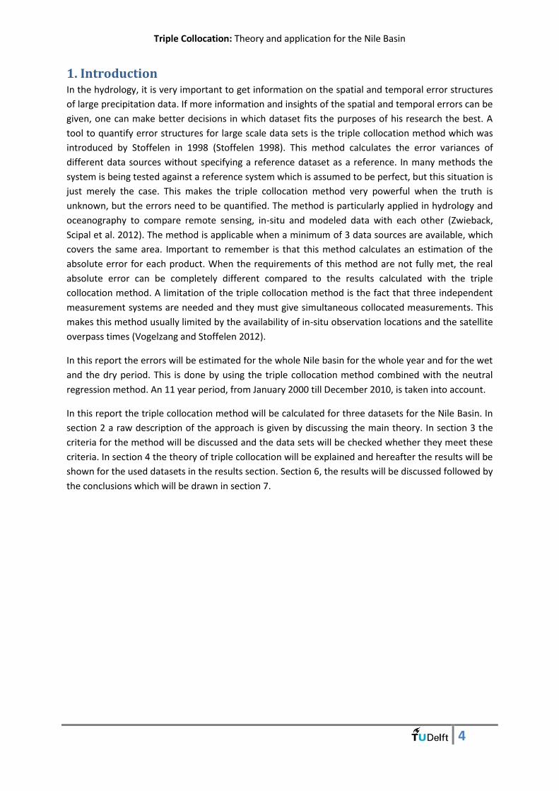
Triple Collocation: Theory and application for the Nile Basin

4

1. Introduction In the hydrology, it is very important to get information on the spatial and temporal error structures

of large precipitation data. If more information and insights of the spatial and temporal errors can be

given, one can make better decisions in which dataset fits the purposes of his research the best. A

tool to quantify error structures for large scale data sets is the triple collocation method which was

introduced by Stoffelen in 1998 (Stoffelen 1998). This method calculates the error variances of

different data sources without specifying a reference dataset as a reference. In many methods the

system is being tested against a reference system which is assumed to be perfect, but this situation is

just merely the case. This makes the triple collocation method very powerful when the truth is

unknown, but the errors need to be quantified. The method is particularly applied in hydrology and

oceanography to compare remote sensing, in-situ and modeled data with each other (Zwieback,

Scipal et al. 2012). The method is applicable when a minimum of 3 data sources are available, which

covers the same area. Important to remember is that this method calculates an estimation of the

absolute error for each product. When the requirements of this method are not fully met, the real

absolute error can be completely different compared to the results calculated with the triple

collocation method. A limitation of the triple collocation method is the fact that three independent

measurement systems are needed and they must give simultaneous collocated measurements. This

makes this method usually limited by the availability of in-situ observation locations and the satellite

overpass times (Vogelzang and Stoffelen 2012).

In this report the errors will be estimated for the whole Nile basin for the whole year and for the wet

and the dry period. This is done by using the triple collocation method combined with the neutral

regression method. An 11 year period, from January 2000 till December 2010, is taken into account.

In this report the triple collocation method will be calculated for three datasets for the Nile Basin. In

section 2 a raw description of the approach is given by discussing the main theory. In section 3 the

criteria for the method will be discussed and the data sets will be checked whether they meet these

criteria. In section 4 the theory of triple collocation will be explained and hereafter the results will be

shown for the used datasets in the results section. Section 6, the results will be discussed followed by

the conclusions which will be drawn in section 7.

Triple Collocation: Theory and application for the Nile Basin

5

Triple Collocation: Theory and application for the Nile Basin

6

2. Method Pairs of observations are usually not enough to give a good estimation of the errors of each product,

therefore a multiple collocation analysis can be done to give some insight in the absolute error of

each product (Abdalla, Janssen et al. 2011). The method used in this report to give insight in the

errors of six datasets, is by estimating the errors by using the triple collocation method. This method

defines a truth from three input datasets and calculates the associated errors at every time or

location for each dataset; this is also shown in Figure 1. These estimated errors are then calibrated by

using the neutral regression approach of Deming which is described in a couple of papers (Mandel

1964, Marsden 1999). This approach is based on the minimization of the errors between the

estimated truth and the datasets. This neutral regression will adjust the dataset a bit in order to

decrease the systematic error part in the estimated errors. The recalibrated dataset is then used as

new input to estimate the errors with the triple collocation again. This interpolation process is

continued until convergence is obtained (Janssen, Abdalla et al. 2007). So in every iteration step the

datasets are adjusted by the neutral regression approach and the new truth will be defined and

errors are calculated by the triple collocation method. Some criteria must be met when a triple

collocation is applied in order to get accurate error estimations. Those criteria are given and

discussed in section 3 and the mathematical description is shown in the next section 4 of this report.

Figure 1: The estimated truth and errors calculated by the triple collocation method

Triple Collocation: Theory and application for the Nile Basin

7

Triple Collocation: Theory and application for the Nile Basin

8

3. Criteria for the method For triple collocation a couple of criteria must be met. The main criteria are summed bellow:

1. Three datasets are needed to do the comparison

2. The random errors must be uncorrelated

3. The datasets must be correlated to each other

4. The datasets must be biased corrected

5. The errors are assumed to be Gaussian distributed

In the remaining of this section those criteria will be discussed one by one.

3.1. Criteria 1 The triple collocation method needs a minimum of three datasets to do the comparison. A criterion is

that those datasets must also involve the same spatial and temporal scale. For many datasets this

can be a problem but for satellite datasets which are used in this report, this criterion is not the most

difficult criterion to meet. This is because of the globally and spatially coverage of the satellites,

resulting that all datasets can have the same monthly scale and cover the same area.

3.2. Criteria 2 A more difficult criterion to fulfill is that the random errors must be uncorrelated. This difficulty is

due to the same sensors that are involved in the different datasets; this makes the random errors

correlated resulting that the triple collocation cannot be applied when two of those datasets are

involved. When all the datasets are compared to each other one can find indeed three different

datasets, which use different sensors and methods to come up with the rainfall product. Therefore,

the triple collocation can be applied with those datasets. The first dataset is the CRU_TS3.21 dataset,

which uses solely ground point measurements which are extrapolated by using the Climate Anomaly

Method and is interpolated to a grid with a triangulated linear interpolation technique. The second

dataset is the ECMWF model for rainfall. This model uses a lot of different input data, which also

includes the satellite sensor data and many more other data sources like data from weather stations

on the land and the ocean, data from ships, airplanes, buoys, and many other data sources. All this

collected data is used as input for the model which calculates many hydrologic parameters, like

humidity, temperature, radiation and rainfall. The third model can be one of the other 10 datasets,

all those datasets includes the sensors from the GEO (geostationary) and/or LEO (low earth orbiting)

satellites. The data set that is used in this report is the RFE 2.0, CHIRPS v1.8, TAMSAT, and

TRMM3B43 v7 dataset. To calculate the errors, an 11 year period is used started from January 2000

to December 2010. The whole Nile Basin is the research area. Another problem is that all those

datasets have different grid sizes. If the three datasets in the triple collocation consist of different

grid sizes, the resulting error estimated with this method will also consist of a sample error which is

also called the representation error. This error can be taken into account as an error correlation

between the two systems which has a higher resolution, but the representation error can also be

minimized by rescaling the finer grid sizes to the coarsest grid size (Roebeling, Wolters et al. 2012).

Therefore, in this report the coarsest grid size is used as standard for the triple collocation. This was

the ECMWF dataset which has a grid size of 0.75 degree. The other datasets are rescaled to this

standard by averaging pixels.

Triple Collocation: Theory and application for the Nile Basin

9

3.3. Criteria 3 Another criterion is that the datasets must be correlated with each other. Therefore, the correlation

is calculated by rescaling the three datasets to a 0.75 grid size. The results are shown in Figure 2. As

one can see is the correlation between the products very high in the wet locations of the Nile Basin.

So this criterion is fulfilled for this area. For the dry areas the correlation is very low, but this is not a

problem because here the yearly rainfall is zero or almost zero. This will result in a very small or no

error output from the triple collocation method and therefore this area does not necessarily need to

have a high correlation between the products.

Figure 2: The correlation coefficient of the used dataset

Triple Collocation: Theory and application for the Nile Basin

10

3.4. Criteria 4 Another criterion for the three datasets is that they all must be bias corrected. This assumption is

fulfilled for most of the datasets, because all datasets are bias corrected by the developers before

making them available for public use. Due to this criteria the third satellite dataset cannot be the

PERSIANN, CMORPH or GSMaP datasets, because those are not biased corrected.

3.5. Criteria 5 The last main criterion is that the errors must be Gaussian distributed with a zero mean. This can be

guaranteed when the errors are calculated for a long time period. The mean of the errors will then

be Gaussian distributed. A time span of 11 year is taken into account so with the consisting 132

months the error can be calculated and be assumed that this is Gaussian distributed. In this report

the year is divided into two periods so in one period 66 months are used to calculate the mean error.

If more periods in a year are chosen, the Gaussian distribution of errors cannot be guaranteed

because too few months are involved. This can be solved by using more years of data.

3.6. Applying triple collocation With respect of those criteria’s stated above, the triple collocation will be applied four times in this

research. The datasets used in those four calculations are:

1. RFE 2.0, CRU_TS3.21, and ECMWF

2. CHIRPS v1.8, CRU_TS3.21, and ECMWF

3. TAMSAT, CRU_TS3.21, and ECMWF

4. TRMM3B43 v7, CRU_TS3.21, and ECMWF

Triple Collocation: Theory and application for the Nile Basin

11

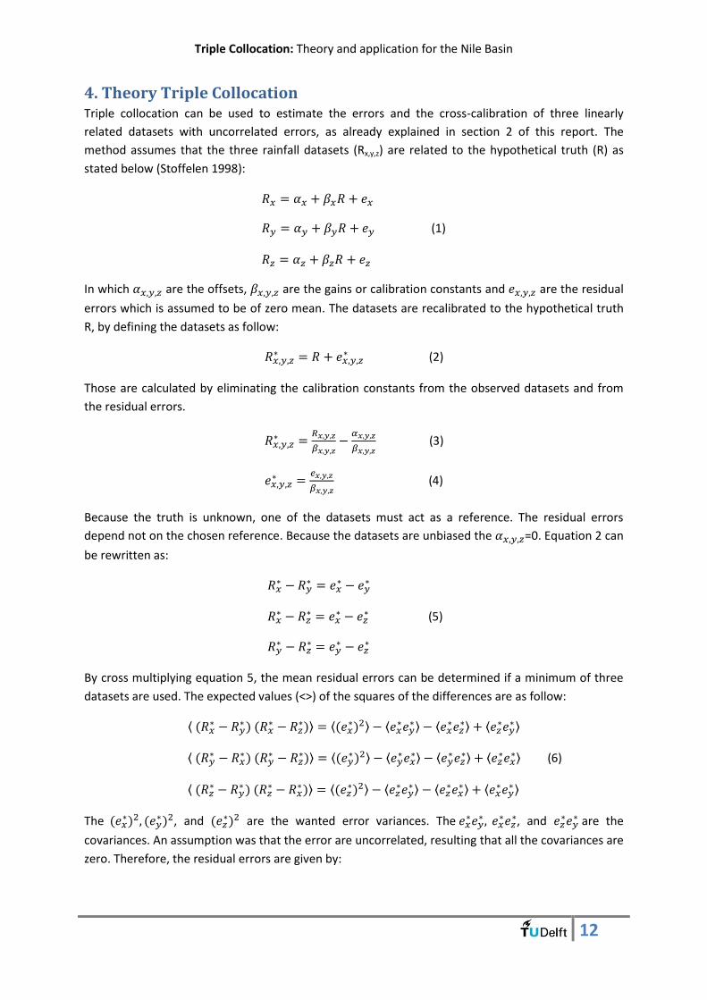
Triple Collocation: Theory and application for the Nile Basin

12

4. Theory Triple Collocation Triple collocation can be used to estimate the errors and the cross-calibration of three linearly

related datasets with uncorrelated errors, as already explained in section 2 of this report. The

method assumes that the three rainfall datasets (Rx,y,z) are related to the hypothetical truth (R) as

stated below (Stoffelen 1998):

(1)

In which are the offsets, are the gains or calibration constants and are the residual

errors which is assumed to be of zero mean. The datasets are recalibrated to the hypothetical truth

R, by defining the datasets as follow:

(2)

Those are calculated by eliminating the calibration constants from the observed datasets and from

the residual errors.

(3)

(4)

Because the truth is unknown, one of the datasets must act as a reference. The residual errors

depend not on the chosen reference. Because the datasets are unbiased the =0. Equation 2 can

be rewritten as:

(5)

By cross multiplying equation 5, the mean residual errors can be determined if a minimum of three

datasets are used. The expected values (<>) of the squares of the differences are as follow:

(6)

The

, and are the wanted error variances. The

, and

are the

covariances. An assumption was that the error are uncorrelated, resulting that all the covariances are

zero. Therefore, the residual errors are given by:

Triple Collocation: Theory and application for the Nile Basin

13

6)

By assuming that dataset x is calibrated , the other two systems can be calibrated by using x

as reference. So by using the neutral regression one can find and . The equations used in the

neutral regression (Marsden 1999) are stated below to calculate the calibration constant (Janssen,

Abdalla et al. 2007):

(7)

Where;

(8)

(9)

(10)

(11)

The can be found by replacing y with z in equation 8 till 11. After those calculations all the

calibration constants are known and one can repeat the whole calculation again but now by using the

calibration constant of equations 3 to adjust the observed rainfall. Repeat those steps until

convergence is obtained, so when all the calibration constants become 1.

With the error, the standard deviation can be calculated by the following relationship between error

and standard deviation:

For this report the means of the errors are taken for every grid for a period of time. A large time

period is needed to guarantee that the mean errors are Gaussian, which is one of the main criteria

for the triple collocation method.

The above calculations are done in Matlab with 1000 iteration steps to ensure convergence. The

results of this calculation are shown in the next section. Those calculations are done for two periods,

namely the wet and the dry period of the Nile basin. The periods are both 6 months and are from

May till October (wet period) and from November till April (dry period). Periods with fewer months

were not possible, to ensure a Gaussian distribution of the errors.

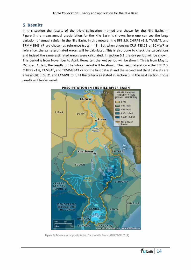
Triple Collocation: Theory and application for the Nile Basin

14

5. Results In this section the results of the triple collocation method are shown for the Nile Basin. In

Figure 3 the mean annual precipitation for the Nile Basin is shown, here one can see the large

variation of annual rainfall in the Nile Basin. In this research the RFE 2.0, CHIRPS v1.8, TAMSAT, and

TRMM3B43 v7 are chosen as reference (so ). But when choosing CRU_TS3.21 or ECMWF as

reference, the same estimated errors will be calculated. This is also done to check the calculations

and indeed the same estimated errors were calculated. In section 5.1 the dry period will be shown.

This period is from November to April. Hereafter, the wet period will be shown. This is from May to

October. At last, the results of the whole period will be shown. The used datasets are the RFE 2.0,

CHIRPS v1.8, TAMSAT, and TRMM3B43 v7 for the first dataset and the second and third datasets are

always CRU_TS3.21 and ECMWF to fulfil the criteria as stated in section 3. In the next section, those

results will be discussed.

Figure 3: Mean annual precipitation for the Nile Basin (STRATFOR 2011)

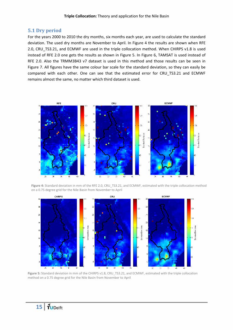
Triple Collocation: Theory and application for the Nile Basin

15

5.1 Dry period For the years 2000 to 2010 the dry months, six months each year, are used to calculate the standard

deviation. The used dry months are November to April. In Figure 4 the results are shown when RFE

2.0, CRU_TS3.21, and ECMWF are used in the triple collocation method. When CHIRPS v1.8 is used

instead of RFE 2.0 one gets the results as shown in Figure 5. In Figure 6, TAMSAT is used instead of

RFE 2.0. Also the TRMM3B43 v7 dataset is used in this method and those results can be seen in

Figure 7. All figures have the same colour bar scale for the standard deviation, so they can easily be

compared with each other. One can see that the estimated error for CRU_TS3.21 and ECMWF

remains almost the same, no matter which third dataset is used.

Figure 5: Standard deviation in mm of the CHIRPS v1.8, CRU_TS3.21, and ECMWF, estimated with the triple collocation method on a 0.75 degree grid for the Nile Basin from November to April

Figure 4: Standard deviation in mm of the RFE 2.0, CRU_TS3.21, and ECMWF, estimated with the triple collocation method on a 0.75 degree grid for the Nile Basin from November to April

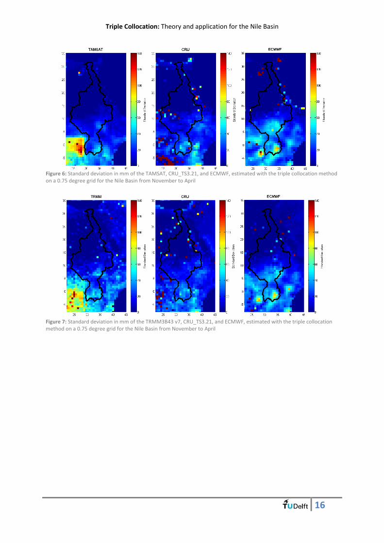
Triple Collocation: Theory and application for the Nile Basin

16

Figure 6: Standard deviation in mm of the TAMSAT, CRU_TS3.21, and ECMWF, estimated with the triple collocation method on a 0.75 degree grid for the Nile Basin from November to April

Figure 7: Standard deviation in mm of the TRMM3B43 v7, CRU_TS3.21, and ECMWF, estimated with the triple collocation method on a 0.75 degree grid for the Nile Basin from November to April

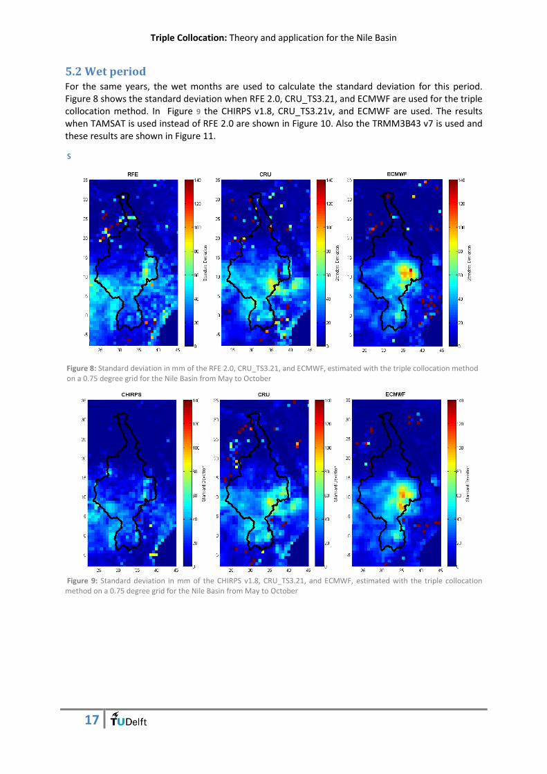
Triple Collocation: Theory and application for the Nile Basin

17

5.2 Wet period For the same years, the wet months are used to calculate the standard deviation for this period. Figure 8 shows the standard deviation when RFE 2.0, CRU_TS3.21, and ECMWF are used for the triple collocation method. In Figure 9 the CHIRPS v1.8, CRU_TS3.21v, and ECMWF are used. The results when TAMSAT is used instead of RFE 2.0 are shown in Figure 10. Also the TRMM3B43 v7 is used and these results are shown in Figure 11.

S

Figure 9: Standard deviation in mm of the CHIRPS v1.8, CRU_TS3.21, and ECMWF, estimated with the triple collocation method on a 0.75 degree grid for the Nile Basin from May to October

Figure 8: Standard deviation in mm of the RFE 2.0, CRU_TS3.21, and ECMWF, estimated with the triple collocation method on a 0.75 degree grid for the Nile Basin from May to October

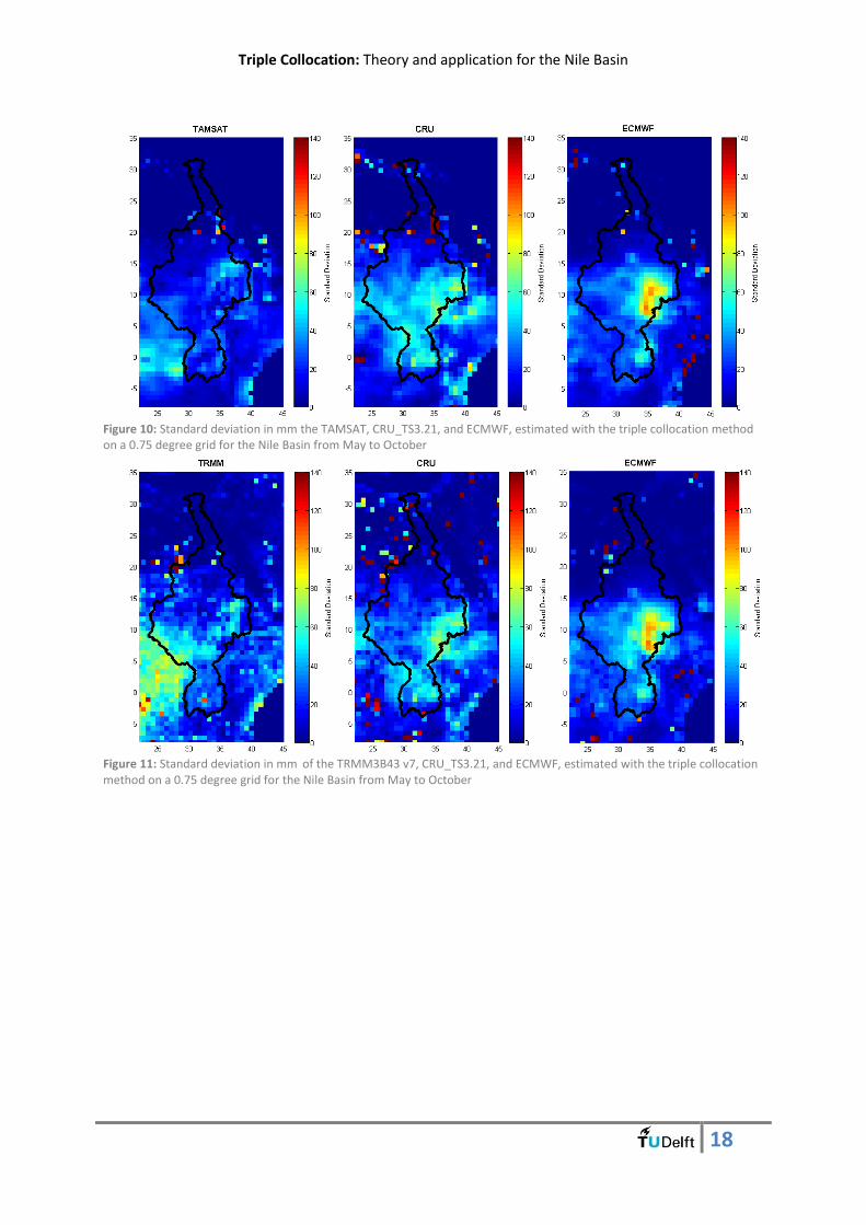
Triple Collocation: Theory and application for the Nile Basin

18

Figure 10: Standard deviation in mm the TAMSAT, CRU_TS3.21, and ECMWF, estimated with the triple collocation method on a 0.75 degree grid for the Nile Basin from May to October

Figure 11: Standard deviation in mm

of the TRMM3B43 v7, CRU_TS3.21, and ECMWF, estimated with the triple collocation

method on a 0.75 degree grid for the Nile Basin from May to October

Triple Collocation: Theory and application for the Nile Basin

19

5.3 Whole period For the same years, the whole year is considered to calculate the annual standard errors. The same

datasets are used. Only the first dataset is variable and all the results are shown in Figure 12 to Figure

15 for the RFE 2.0, CHIRPS v1.8, TAMSAT and TRMM3B43 v7 respectively as first dataset.

Figure 13: Standard deviation in mm of the CHIRPS v1.8, CRU_TS3.21, and ECMWF, estimated with the triple collocation method on a 0.75 degree grid for the Nile Basin for the whole year

Figure 12: Standard deviation in mm of the RFE 2.0, CRU_TS3.21, and ECMWF, estimated with the triple collocation method on a 0.75 degree grid for the Nile Basin for the whole year

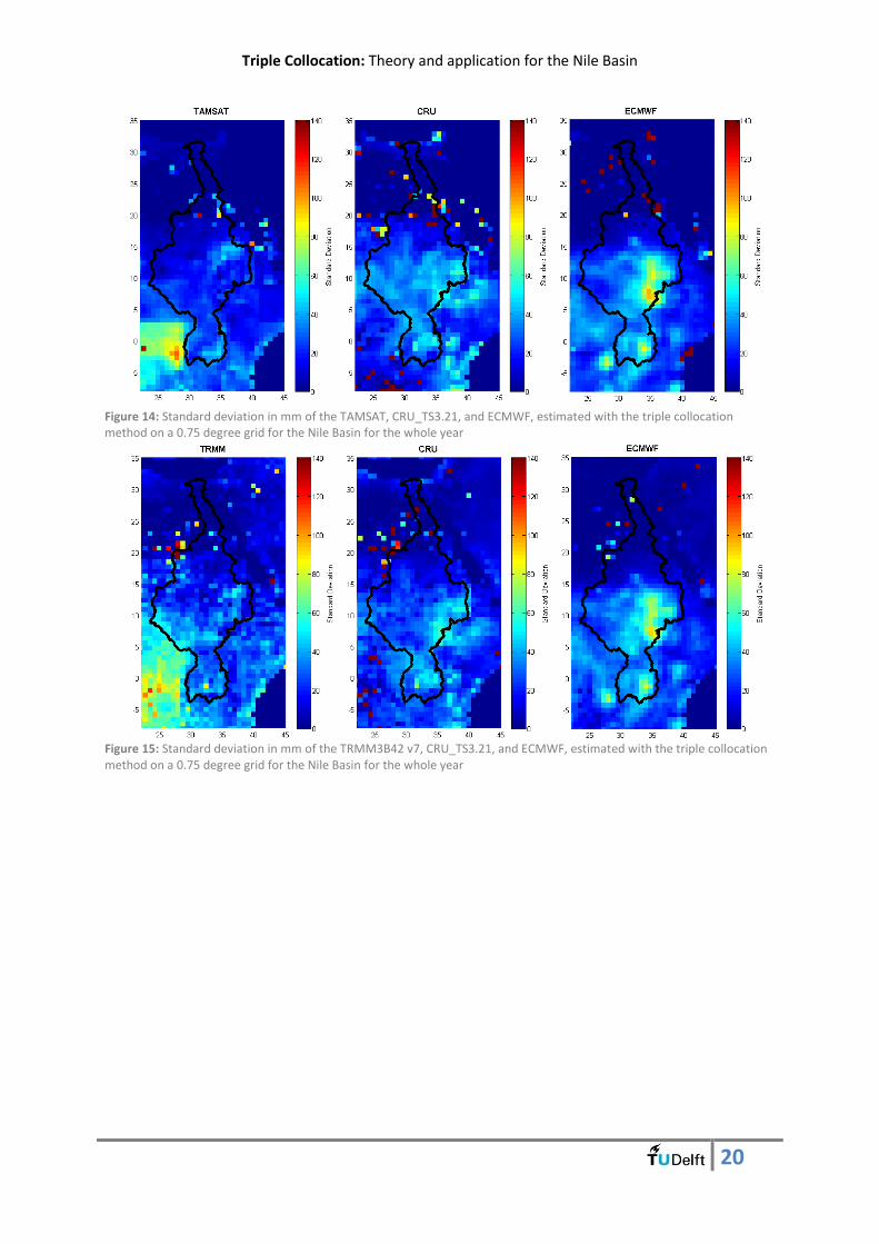
Triple Collocation: Theory and application for the Nile Basin

20

Figure 14: Standard deviation in mm of the TAMSAT, CRU_TS3.21, and ECMWF, estimated with the triple collocation method on a 0.75 degree grid for the Nile Basin for the whole year

Figure 15: Standard deviation in mm of the TRMM3B42 v7, CRU_TS3.21, and ECMWF, estimated with the triple collocation method on a 0.75 degree grid for the Nile Basin for the whole year

Triple Collocation: Theory and application for the Nile Basin

21

6. Discussion For the validity of the derived error model, two assumptions are important. Firstly, the residual

errors need to be uncorrelated and secondly, there must be linear relations between the three

datasets (Roebeling, Wolters et al. 2012). The first assumption is not completely fulfilled, because the

datasets do not use completely different datasets as input for their rainfall estimations. But all the

datasets use different retrieval techniques. The ECMWF uses a lot of input data like buoys, airplanes,

dropsondes, radiosondes, but also the geostationary and the passive microwave sensors that are also

used in the CHIRPS v1.8, RFE 2.0, TAMSAT and TRMM3B43 v7 rainfall estimates. Because the ECMWF

uses a lot of different data sources as input data for a model, the assumption was made that the

ECMWF is completely different than the CHIRPS v1.8, RFE 2.0, TAMSAT, and TRMM3B43 v7

estimations which uses just the geostationary and passive microwave sensors and calculate rainfall

by using a retrieval algorithm. As a result, it is assumed that the residual errors are uncorrelated, so

the errors resulting from the use of the same sensors are assumed to be negligible. The second is not

completely fulfilled if a 0.05 degree grid is used because the sampling resolutions are different, so it

might be necessary to use a more sophisticated calibration approach to minimize the systematic

errors. Here the datasets are just rescaled to the dataset with the coarsest grid to minimize the

residual errors. This is shown in the estimated error on a 0.75 degree grid. Therefore, this assumption

is also fulfilled.

One can see that the places where the correlations between products were zero or almost zero, the

resulting estimated error is also zero. These are also the areas where no rain is detected, so this area

is not very important for this analysis. Furthermore, some pixels have strange values. In those areas

no convergence was reached. This can have two reasons; the first reason is that more iteration steps

are needed to reach convergence. The second reason is that convergence cannot be reached due to

low correlation between the datasets. The strange pixels are especially located in the areas which are

characterized as the areas with a low correlation factor. Therefore, the second reason is most

reasonable for most pixels.

When one takes a look at the dry period one can see that the standard deviations in the Nile basin

are low. This is due to the smaller amount of rain during this period. In general, the ECMWF has the

larger standard deviations in the Nile basin especially in the southern part compared with the other

datasets. The RFE 2.0 has some problems at latitude of 7N and longitude of 35E, and also TAMSAT,

TRMM3B43 v7, and ECMWF has some larger standard deviations in this particular area. In general,

the CRU_TS3.21, TAMSAT, and CHIRPS v1.8 have the lowest errors when only the Nile basin is taking

into account. All the datasets have the largest errors in the southern part of the Nile Basin, so around

Lake Victoria. On the left side just outside the Nile basin, one can see a large standard deviation for

the TRMM3B43 v7 and TAMSAT database. In general one can conclude that the CHIRPS v1.8,

TAMSAT and CRU_TS3.21 have the lowest mean standard deviation when the whole Nile Basin is

taken into account, but on local scale also other datasets can have a lower error.

In the wet period the ECMWF has a large standard deviation in the right center of the Nile Basin (35E

latitude, 10N longitude), this is the Baro-Akobo-Sobat region in which a lot of researches concluded

that the ECMWF overestimates the rainfall extremely in this area(Thiemig, Rojas et al. 2012). Also

CRU_TS3.21 has some larger errors in this particular area. The TRMM3B42 v7 has a larger standard

deviation in the whole center part compared to the CHIRPS v1.8, TAMSAT, and RFE 2.0. In the

southern part of the Nile Basin, the TAMSAT and the CHIRPS v1.8 has the lowest standard deviation

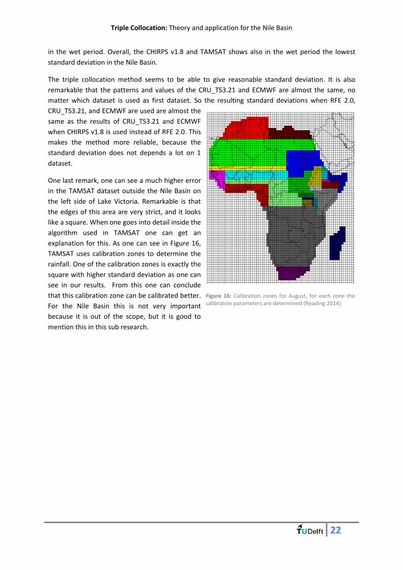
Triple Collocation: Theory and application for the Nile Basin

22

in the wet period. Overall, the CHIRPS v1.8 and TAMSAT shows also in the wet period the lowest

standard deviation in the Nile Basin.

The triple collocation method seems to be able to give reasonable standard deviation. It is also

remarkable that the patterns and values of the CRU_TS3.21 and ECMWF are almost the same, no

matter which dataset is used as first dataset. So the resulting standard deviations when RFE 2.0,

CRU_TS3.21, and ECMWF are used are almost the

same as the results of CRU_TS3.21 and ECMWF

when CHIRPS v1.8 is used instead of RFE 2.0. This

makes the method more reliable, because the

standard deviation does not depends a lot on 1

dataset.

One last remark, one can see a much higher error

in the TAMSAT dataset outside the Nile Basin on

the left side of Lake Victoria. Remarkable is that

the edges of this area are very strict, and it looks

like a square. When one goes into detail inside the

algorithm used in TAMSAT one can get an

explanation for this. As one can see in Figure 16,

TAMSAT uses calibration zones to determine the

rainfall. One of the calibration zones is exactly the

square with higher standard deviation as one can

see in our results. From this one can conclude

that this calibration zone can be calibrated better.

For the Nile Basin this is not very important

because it is out of the scope, but it is good to

mention this in this sub research.

Figure 16: Calibration zones for August, for each zone the calibration parameters are determined (Reading 2014)

Triple Collocation: Theory and application for the Nile Basin

23

6. Summary The triple collocation is a powerful tool to give insight in the error when the truth is unknown. With

this method, it is possible to make an estimation of the error, but it is important to take care of the

many criteria which have to be fulfilled before this method is able to estimate the errors accurately.

Because of those criteria, the possibility of using some datasets or the combination of some datasets

is not possible without introducing an additional error in your error estimation calculations. For this

research, those criteria results in the obligation of using the ECMWF and CRU_TS3.21 datasets and

that only the third dataset is the only variable dataset. This third dataset, one can choose between

the RFE 2.0, TRMM3B43 v7, CHIRPS v1.8, and the TAMSAT dataset. So the use of this method is

limited and not all the datasets or a combination of datasets can be used.

The result of triple collocation shows some useful information which seems to be very plausible. The

standard deviation of the ECMWF and CRU_TS3.21 does not depend much on the input data of the

third database. So one gets almost the same standard deviation for ECMWF and CRU_TS3.21 if RFE

2.0, ECMWF, and CRU_TS3.21 are used as when CHIRPS v1.8 is used instead of RFE 2.0.

The first dataset (RFE 2.0, CHIRPS v1.8, TAMSAT, or TRMM3B43 v7) is chosen as reference for the

triple collocation, but when CRU_TS3.21 or ECMWF is chosen as reference; by definition the same

estimated errors must be calculated. So to check the calculations also the other two datasets were

chosen as reference system, which resulted in the same estimated errors.

From this analysis one can conclude in general that the CHIRPS v1.8, CRU_TS3.21, and TAMSAT have

the lowest standard deviation inside the Nile Basin in the dry season. And for the wet the CHIRPS

v1.8 and TAMSAT shows the lowest standard deviation in general.

Locally, another dataset than mentioned above can have a lower standard deviation.

This result can be used to make an ensemble rainfall product of all the used datasets. With this

result, one can make a decision of which dataset can be used in which area. So for every pixel one

can select the product with the lowest standard deviation.

Triple Collocation: Theory and application for the Nile Basin

24

7. References Abdalla, S., et al. (2011). "Altimeter near real time wind and wave products: Random error estimation." Marine Geodesy 34(3-4): 393-406. Janssen, P. A., et al. (2007). "Error estimation of buoy, satellite, and model wave height data." Journal of Atmospheric and Oceanic Technology 24(9): 1665-1677. Mandel, J. (1964). "The statistical analysis of experimental data." Mineola, NY: Dover Publications 410. Marsden, R. F. (1999). "A proposal for a neutral regression." Journal of Atmospheric and Oceanic Technology 16(7): 876-883. Reading (2014). "TAMSAT." Retrieved 17 June, 2014, from http://www.met.reading.ac.uk/~vm004202/tamsat/. Roebeling, R., et al. (2012). "Triple collocation of summer precipitation retrievals from SEVIRI over Europe with gridded rain gauge and weather radar data." Journal of Hydrometeorology 13(5): 1552-1566. Stoffelen, A. (1998). "Toward the true near‐surface wind speed: Error modeling and calibration using triple collocation." Journal of Geophysical Research: Oceans (1978–2012) 103(C4): 7755-7766. STRATFOR (2011). Precipitation in the Nile River Basin. Dec.-16-nile-precipitation2.jpg. www.STRATFOR.com, STRATFOR. Thiemig, V., et al. (2012). "Validation of satellite-based precipitation products over sparsely gauged African river basins." Journal of Hydrometeorology 13(6): 1760-1783. Vogelzang, J. and A. Stoffelen (2012). "Triple collocation." Zwieback, S., et al. (2012). "Structural and statistical properties of the collocation technique for error characterization." Nonlinear Processes in Geophysics 19(1): 69-80.

Triple Collocation: Theory and application for the Nile Basin

25

Matlab m-files M-files used for the scientific paper

TU Delft Tim M. Hessels Supervisor: Prof. Dr. Wim G.M.Bastiaanssen

Matlab m-files: m-files used for the scientific paper

1

Matlab m-files: m-files used for the scientific paper

2

0. Introduction ......................................................................................................................................... 4

1. Open access product ........................................................................................................................... 5

1.1 Making clipped .tiff files from products ....................................................................................... 5

1.1.1 TRMM ..................................................................................................................................... 5

1.1.2 GPCP ....................................................................................................................................... 6

1.1.3 GPCP1DD ................................................................................................................................ 6

1.1.4 CRU ......................................................................................................................................... 7

1.1.5 ECMWF ................................................................................................................................... 7

1.1.6 ARC ......................................................................................................................................... 8

1.1.7 CHIRPS .................................................................................................................................... 9

1.1.8 RFE .......................................................................................................................................... 9

1.1.9 TAMSAT ................................................................................................................................ 11

1.1.10 GSMaP ................................................................................................................................ 11

1.1.11 PERSIANN ........................................................................................................................... 15

1.1.12 CMORPH ............................................................................................................................. 26

1.1.13 GPCC ................................................................................................................................... 27

1.2 Clipping the data ......................................................................................................................... 27

1.3 Visualizing the products .............................................................................................................. 29

1.3.1 Average for each basin and subbasin of each product. ....................................................... 29

1.3.2 Difference between point measurements ........................................................................... 34

1.3.3 Boxplot graphs ...................................................................................................................... 40

1.3.4 Total Yearly Rainfall .............................................................................................................. 42

2. Ground Measurements ..................................................................................................................... 48

3. Triple Collocation product ................................................................................................................. 51

4. Prepare maps for validation .............................................................................................................. 62

4.1 Spatial resolution of the products ............................................................................................... 62

4.2 Select pixels which are used for the validation ........................................................................... 66

5. Interpolation techniques ................................................................................................................... 68

5.1 Simple averaging ......................................................................................................................... 68

5.1.1 yearly simple averaging ........................................................................................................ 68

5.1.2 Monthly simple averaging .................................................................................................... 71

5.1.3 Visualizing monthly rainfall correlation, RMSE, and bias ..................................................... 75

5.2 Variable averaging ....................................................................................................................... 79

5.2.1 Yearly variable averaging...................................................................................................... 79

Matlab m-files: m-files used for the scientific paper

3

5.2.1 Monthly variable averaging .................................................................................................. 85

5.3 Block kriging ................................................................................................................................ 90

5.3.1 Fit semivariograms ............................................................................................................... 90

5.3.2 Interpolate ground measurements using block kriging ....................................................... 92

5.3.3 Comparison between Block kriging and products ................................................................ 95

5.3.4 Validation using the block kriging method ........................................................................... 97

6. Pictures in paper .............................................................................................................................. 100

6.1 Figure 1: ..................................................................................................................................... 100

6.2 Figure 2: ..................................................................................................................................... 100

6.3 Figure 3: ..................................................................................................................................... 100

6.4 Figure 4: ..................................................................................................................................... 100

6.5 Figure 5: ..................................................................................................................................... 101

6.6 Figure 6: ..................................................................................................................................... 102

6.7 Figure 7: ..................................................................................................................................... 106

6.8 Figure 8: ..................................................................................................................................... 107

7. Webpages for downloading rainfall data ........................................................................................ 108

Matlab m-files: m-files used for the scientific paper

4

0. Introduction In this report all the m-file which are used for the scientific paper are shown. More analysis were

done, but they were not published in the paper and therefore those m-files are not shown in this

report. In the figure below the content of this report is shown.

Blue parts in the m-files say something about the data input of that command. So from where this

data is downloaded or with which m-file this data is calculated.

In section 7, all the website and FTP servers are shown from where all the rainfall data used in this

study is downloaded.

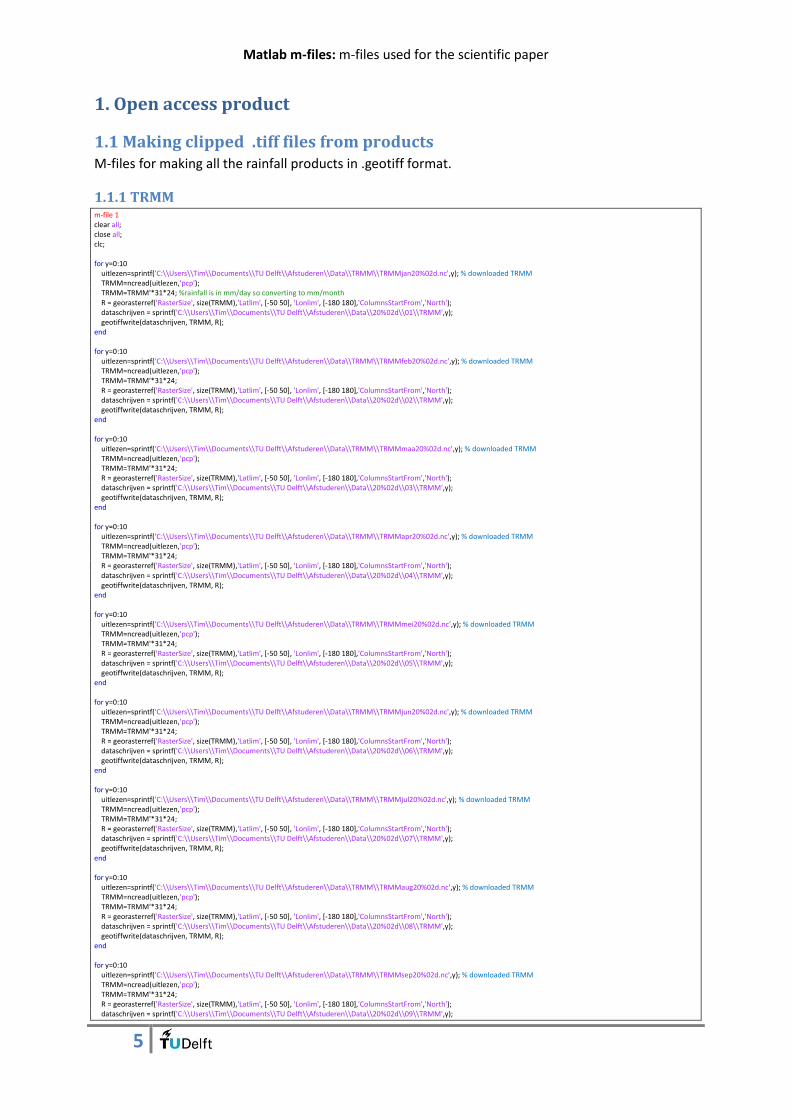
Matlab m-files: m-files used for the scientific paper

5

1. Open access product

1.1 Making clipped .tiff files from products M-files for making all the rainfall products in .geotiff format.

1.1.1 TRMM m-file 1 clear all; close all; clc; for y=0:10 uitlezen=sprintf('C:\\Users\\Tim\\Documents\\TU Delft\\Afstuderen\\Data\\TRMM\\TRMMjan20%02d.nc',y); % downloaded TRMM TRMM=ncread(uitlezen,'pcp'); TRMM=TRMM'*31*24; %rainfall is in mm/day so converting to mm/month R = georasterref('RasterSize', size(TRMM),'Latlim', [-50 50], 'Lonlim', [-180 180],'ColumnsStartFrom','North'); dataschrijven = sprintf('C:\\Users\\Tim\\Documents\\TU Delft\\Afstuderen\\Data\\20%02d\\01\\TRMM',y); geotiffwrite(dataschrijven, TRMM, R); end for y=0:10 uitlezen=sprintf('C:\\Users\\Tim\\Documents\\TU Delft\\Afstuderen\\Data\\TRMM\\TRMMfeb20%02d.nc',y); % downloaded TRMM TRMM=ncread(uitlezen,'pcp'); TRMM=TRMM'*31*24; R = georasterref('RasterSize', size(TRMM),'Latlim', [-50 50], 'Lonlim', [-180 180],'ColumnsStartFrom','North'); dataschrijven = sprintf('C:\\Users\\Tim\\Documents\\TU Delft\\Afstuderen\\Data\\20%02d\\02\\TRMM',y); geotiffwrite(dataschrijven, TRMM, R); end for y=0:10 uitlezen=sprintf('C:\\Users\\Tim\\Documents\\TU Delft\\Afstuderen\\Data\\TRMM\\TRMMmaa20%02d.nc',y); % downloaded TRMM TRMM=ncread(uitlezen,'pcp'); TRMM=TRMM'*31*24; R = georasterref('RasterSize', size(TRMM),'Latlim', [-50 50], 'Lonlim', [-180 180],'ColumnsStartFrom','North'); dataschrijven = sprintf('C:\\Users\\Tim\\Documents\\TU Delft\\Afstuderen\\Data\\20%02d\\03\\TRMM',y); geotiffwrite(dataschrijven, TRMM, R); end for y=0:10 uitlezen=sprintf('C:\\Users\\Tim\\Documents\\TU Delft\\Afstuderen\\Data\\TRMM\\TRMMapr20%02d.nc',y); % downloaded TRMM TRMM=ncread(uitlezen,'pcp'); TRMM=TRMM'*31*24; R = georasterref('RasterSize', size(TRMM),'Latlim', [-50 50], 'Lonlim', [-180 180],'ColumnsStartFrom','North'); dataschrijven = sprintf('C:\\Users\\Tim\\Documents\\TU Delft\\Afstuderen\\Data\\20%02d\\04\\TRMM',y); geotiffwrite(dataschrijven, TRMM, R); end for y=0:10 uitlezen=sprintf('C:\\Users\\Tim\\Documents\\TU Delft\\Afstuderen\\Data\\TRMM\\TRMMmei20%02d.nc',y); % downloaded TRMM TRMM=ncread(uitlezen,'pcp'); TRMM=TRMM'*31*24; R = georasterref('RasterSize', size(TRMM),'Latlim', [-50 50], 'Lonlim', [-180 180],'ColumnsStartFrom','North'); dataschrijven = sprintf('C:\\Users\\Tim\\Documents\\TU Delft\\Afstuderen\\Data\\20%02d\\05\\TRMM',y); geotiffwrite(dataschrijven, TRMM, R); end for y=0:10 uitlezen=sprintf('C:\\Users\\Tim\\Documents\\TU Delft\\Afstuderen\\Data\\TRMM\\TRMMjun20%02d.nc',y); % downloaded TRMM TRMM=ncread(uitlezen,'pcp'); TRMM=TRMM'*31*24; R = georasterref('RasterSize', size(TRMM),'Latlim', [-50 50], 'Lonlim', [-180 180],'ColumnsStartFrom','North'); dataschrijven = sprintf('C:\\Users\\Tim\\Documents\\TU Delft\\Afstuderen\\Data\\20%02d\\06\\TRMM',y); geotiffwrite(dataschrijven, TRMM, R); end for y=0:10 uitlezen=sprintf('C:\\Users\\Tim\\Documents\\TU Delft\\Afstuderen\\Data\\TRMM\\TRMMjul20%02d.nc',y); % downloaded TRMM TRMM=ncread(uitlezen,'pcp'); TRMM=TRMM'*31*24; R = georasterref('RasterSize', size(TRMM),'Latlim', [-50 50], 'Lonlim', [-180 180],'ColumnsStartFrom','North'); dataschrijven = sprintf('C:\\Users\\Tim\\Documents\\TU Delft\\Afstuderen\\Data\\20%02d\\07\\TRMM',y); geotiffwrite(dataschrijven, TRMM, R); end for y=0:10 uitlezen=sprintf('C:\\Users\\Tim\\Documents\\TU Delft\\Afstuderen\\Data\\TRMM\\TRMMaug20%02d.nc',y); % downloaded TRMM TRMM=ncread(uitlezen,'pcp'); TRMM=TRMM'*31*24; R = georasterref('RasterSize', size(TRMM),'Latlim', [-50 50], 'Lonlim', [-180 180],'ColumnsStartFrom','North'); dataschrijven = sprintf('C:\\Users\\Tim\\Documents\\TU Delft\\Afstuderen\\Data\\20%02d\\08\\TRMM',y); geotiffwrite(dataschrijven, TRMM, R); end for y=0:10 uitlezen=sprintf('C:\\Users\\Tim\\Documents\\TU Delft\\Afstuderen\\Data\\TRMM\\TRMMsep20%02d.nc',y); % downloaded TRMM TRMM=ncread(uitlezen,'pcp'); TRMM=TRMM'*31*24; R = georasterref('RasterSize', size(TRMM),'Latlim', [-50 50], 'Lonlim', [-180 180],'ColumnsStartFrom','North'); dataschrijven = sprintf('C:\\Users\\Tim\\Documents\\TU Delft\\Afstuderen\\Data\\20%02d\\09\\TRMM',y);

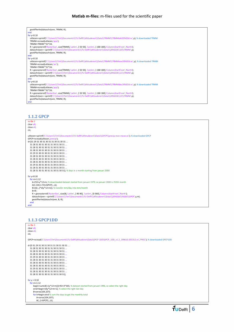
Matlab m-files: m-files used for the scientific paper

6

geotiffwrite(dataschrijven, TRMM, R); end for y=0:10 uitlezen=sprintf('C:\\Users\\Tim\\Documents\\TU Delft\\Afstuderen\\Data\\TRMM\\TRMMokt20%02d.nc',y); % downloaded TRMM TRMM=ncread(uitlezen,'pcp'); TRMM=TRMM'*31*24; R = georasterref('RasterSize', size(TRMM),'Latlim', [-50 50], 'Lonlim', [-180 180],'ColumnsStartFrom','North'); dataschrijven = sprintf('C:\\Users\\Tim\\Documents\\TU Delft\\Afstuderen\\Data\\20%02d\\10\\TRMM',y); geotiffwrite(dataschrijven, TRMM, R); end for y=0:10 uitlezen=sprintf('C:\\Users\\Tim\\Documents\\TU Delft\\Afstuderen\\Data\\TRMM\\TRMMnov20%02d.nc',y); % downloaded TRMM TRMM=ncread(uitlezen,'err'); TRMM=TRMM'*31*24; R = georasterref('RasterSize', size(TRMM),'Latlim', [-50 50], 'Lonlim', [-180 180],'ColumnsStartFrom','North'); dataschrijven = sprintf('C:\\Users\\Tim\\Documents\\TU Delft\\Afstuderen\\Data\\20%02d\\11\\TRMM',y); geotiffwrite(dataschrijven, TRMM, R); end for y=0:10 uitlezen=sprintf('C:\\Users\\Tim\\Documents\\TU Delft\\Afstuderen\\Data\\TRMM\\TRMMdec20%02d.nc',y); % downloaded TRMM TRMM=ncread(uitlezen,'pcp'); TRMM=TRMM'*31*24; R = georasterref('RasterSize', size(TRMM),'Latlim', [-50 50], 'Lonlim', [-180 180],'ColumnsStartFrom','North'); dataschrijven = sprintf('C:\\Users\\Tim\\Documents\\TU Delft\\Afstuderen\\Data\\20%02d\\12\\TRMM',y); geotiffwrite(dataschrijven, TRMM, R); end

1.1.2 GPCP m-file 2 clear all; close all; clc; uitlezen=sprintf('C:\\Users\\Tim\\Documents\\TU Delft\\Afstuderen\\Data\\GPCP\\precip.mon.mean.nc'); % downloaded GPCP GPCP=ncread(uitlezen,'precip'); d=[31 29 31 30 31 30 31 31 30 31 30 31 ... 31 28 31 30 31 30 31 31 30 31 30 31 ... 31 28 31 30 31 30 31 31 30 31 30 31 ... 31 28 31 30 31 30 31 31 30 31 30 31 ... 31 29 31 30 31 30 31 31 30 31 30 31 ... 31 28 31 30 31 30 31 31 30 31 30 31 ... 31 28 31 30 31 30 31 31 30 31 30 31 ... 31 28 31 30 31 30 31 31 30 31 30 31 ... 31 29 31 30 31 30 31 31 30 31 30 31 ... 31 28 31 30 31 30 31 31 30 31 30 31 ... 31 28 31 30 31 30 31 31 30 31 30 31]; % days in a month starting from januari 2000 for y=0:10 for m=1:12 k=252+y*12+m; % downloaded dataset started from januari 1979, so januari 2000 is 252th month A(1:144,1:72)=GPCP(:,:,k); B=(A(:,:)*d(y*12+m)); % transfer mm/day into mm/month B=B'; R = georasterref('RasterSize', size(B),'Latlim', [-90 90], 'Lonlim', [0 360],'ColumnsStartFrom','North'); dataschrijven = sprintf('C:\\Users\\Tim\\Documents\\TU Delft\\Afstuderen\\Data\\20%02d\\%02d\\GPCP',y,m); geotiffwrite(dataschrijven, B, R); end end

1.1.3 GPCP1DD m-file 3 clear all; close all; clc; GPCP=ncread('C:\Users\Tim\Documents\TU Delft\Afstuderen\Data\GPCP 1DD\GPCP_1DD_v1.2_199610-201312.nc','PREC'); % downloaded GPCP1DD d=[0 31 29 31 30 31 30 31 31 30 31 30 31 ... 31 28 31 30 31 30 31 31 30 31 30 31 ... 31 28 31 30 31 30 31 31 30 31 30 31 ... 31 28 31 30 31 30 31 31 30 31 30 31 ... 31 29 31 30 31 30 31 31 30 31 30 31 ... 31 28 31 30 31 30 31 31 30 31 30 31 ... 31 28 31 30 31 30 31 31 30 31 30 31 ... 31 28 31 30 31 30 31 31 30 31 30 31 ... 31 29 31 30 31 30 31 31 30 31 30 31 ... 31 28 31 30 31 30 31 31 30 31 30 31 ... 31 28 31 30 31 30 31 31 30 31 30 31]; for y = 0:10 for m=1:12 begin=sum(d(1:(y*12+m)))+92+3*365; % dataset started from januari 1996, so select the right day eind=begin+d(y*12+m+1); % select the right last day B=zeros(104,107); for k=begin:eind % sum the days to get the monthly total A=zeros(104,107); A(:,:)=GPCP(:,:,k);

Matlab m-files: m-files used for the scientific paper

7

B=A+B; end C=B; R = georasterref('RasterSize', size(C),'Latlim', [-90 90], 'Lonlim', [0 360],'ColumnsStartFrom','north'); dataschrijven = sprintf('C:\\Users\\Tim\\Documents\\TU Delft\\Afstuderen\\Data\\20%02d\\%02d\\GPCP1DD',y,m); geotiffwrite(dataschrijven, C, R); end end

1.1.4 CRU m-file 4 clear all; close all; clc; %dataset 1 from 1991 till 2000 uitlezen=sprintf('C:\\Users\\Tim\\Documents\\TU Delft\\Afstuderen\\Data\\CRU\\cru_ts3.21.1991.2000.pre.dat.nc'); % downloaded CRU CRU=ncread(uitlezen,'pre'); %dataset 2 from 2001 till 2010 uitlezen=sprintf('C:\\Users\\Tim\\Documents\\TU Delft\\Afstuderen\\Data\\CRU\\cru_ts3.21.2001.2010.pre.dat.nc'); % downloaded CRU CRU2=ncread(uitlezen,'pre'); %for dataset 1 y=0; for m=1:12 k=(108+m); A(1:720,1:360)=CRU(:,:,k); B=A'; R = georasterref('RasterSize', size(B),'Latlim', [-90 90], 'Lonlim', [0 360]); mapshow(B,R,'DisplayType', 'Texturemap') dataschrijven = sprintf('C:\\Users\\Tim\\Documents\\TU Delft\\Afstuderen\\Data\\20%02d\\%02d\\CRU',y,m); geotiffwrite(dataschrijven, B, R); end %for dataset 2 for y=1:10 for m=1:12 k=(12*(y-1)+m); C(1:720,1:360)=CRU2(:,:,k); D=C'; R = georasterref('RasterSize', size(D),'Latlim', [-90 90], 'Lonlim', [-180 180]); mapshow(D,R,'DisplayType', 'Texturemap') dataschrijven = sprintf('C:\\Users\\Tim\\Documents\\TU Delft\\Afstuderen\\Data\\20%02d\\%02d\\CRU',y,m); geotiffwrite(dataschrijven, D, R); mapshow(D,R,'DisplayType', 'Texturemap') end end

1.1.5 ECMWF m-file 5 clear all; close all; clc; [ECMWF R]=geotiffread('C:\Users\Tim\Documents\TU Delft\Afstuderen\Data\ECMWF\ECMWFalle'); % downloaded ECMWF d=[31 29 31 30 31 30 31 31 30 31 30 31 ... 31 28 31 30 31 30 31 31 30 31 30 31 ... 31 28 31 30 31 30 31 31 30 31 30 31 ... 31 28 31 30 31 30 31 31 30 31 30 31 ... 31 29 31 30 31 30 31 31 30 31 30 31 ... 31 28 31 30 31 30 31 31 30 31 30 31 ... 31 28 31 30 31 30 31 31 30 31 30 31 ... 31 28 31 30 31 30 31 31 30 31 30 31 ... 31 29 31 30 31 30 31 31 30 31 30 31 ... 31 28 31 30 31 30 31 31 30 31 30 31 ... 31 28 31 30 31 30 31 31 30 31 30 31]; for y = 0:10 for m=1:12 begin=sum(d(1:(y*12+m-1)))+1; eind=begin+d(y*12+m); B=zeros(104,107); for k=begin:eind; A=zeros(104,107); A(:,:)=ECMWF(:,:,k); B=A+B; end C=1000*B; R = georasterref('RasterSize', size(C),'Latlim', [-38.625 39.375], 'Lonlim', [-21.375 58.875],'ColumnsStartFrom','north'); dataschrijven = sprintf('C:\\Users\\Tim\\Documents\\TU Delft\\Afstuderen\\Data\\20%02d\\%02d\\ECMWF',y,m); geotiffwrite(dataschrijven, C, R); end end

Matlab m-files: m-files used for the scientific paper

8

1.1.6 ARC m-file 6 clear all; close all; clc; for f=0:10; d=[1 0 0 0 1 0 0 0 1 0 0 0]; s=d(f+1); % leap year for 2000,2004 en 2008 P=dir('C:\Users\Tim\Documents\TU Delft\Afstuderen\Data\ARC2.0\*.tif'); % downloaded ARC B=zeros(801,751); %% january u=1; for k=1:31; uitlezen=sprintf('C:\\Users\\Tim\\Documents\\TU Delft\\Afstuderen\\Data\\ARC2.0\\africa_arc.20%02d0%d02%d.tif',f,u,k); % downloaded ARC [A,R]=geotiffread(uitlezen); B=A+B; end dataschrijven = sprintf('C:\\Users\\Tim\\Documents\\TU Delft\\Afstuderen\\Data\\20%02d\\%02d\\ARC',f,u); geotiffwrite(dataschrijven, B, R); %% february B=zeros(801,751); u=2; for k=1:28+s; uitlezen=sprintf('C:\\Users\\Tim\\Documents\\TU Delft\\Afstuderen\\Data\\ARC2.0\\africa_arc.20%02d0%d02%d.tif',f,u,k); % downloaded ARC [A,R]=geotiffread(uitlezen); B=A+B; end dataschrijven = sprintf('C:\\Users\\Tim\\Documents\\TU Delft\\Afstuderen\\Data\\20%02d\\%02d\\ARC',f,u); geotiffwrite(dataschrijven, B, R); %% march B=zeros(801,751); u=3; for k=1:31; uitlezen=sprintf('C:\\Users\\Tim\\Documents\\TU Delft\\Afstuderen\\Data\\ARC2.0\\africa_arc.20%02d0%d02%d.tif',f,u,k); % downloaded ARC [A,R]=geotiffread(uitlezen); B=A+B; end dataschrijven = sprintf('C:\\Users\\Tim\\Documents\\TU Delft\\Afstuderen\\Data\\20%02d\\%02d\\ARC',f,u); geotiffwrite(dataschrijven, B, R); %% april B=zeros(801,751); u=4; for k=1:30; uitlezen=sprintf('C:\\Users\\Tim\\Documents\\TU Delft\\Afstuderen\\Data\\ARC2.0\\africa_arc.20%02d0%d02%d.tif',f,u,k); % downloaded ARC [A,R]=geotiffread(uitlezen); B=A+B; end dataschrijven = sprintf('C:\\Users\\Tim\\Documents\\TU Delft\\Afstuderen\\Data\\20%02d\\%02d\\ARC',f,u); geotiffwrite(dataschrijven, B, R); %% may B=zeros(801,751); u=5; for k=1:31; uitlezen=sprintf('C:\\Users\\Tim\\Documents\\TU Delft\\Afstuderen\\Data\\ARC2.0\\africa_arc.20%02d0%d02%d.tif',f,u,k); % downloaded ARC [A,R]=geotiffread(uitlezen); B=A+B; end dataschrijven = sprintf('C:\\Users\\Tim\\Documents\\TU Delft\\Afstuderen\\Data\\20%02d\\%02d\\ARC',f,u); geotiffwrite(dataschrijven, B, R); %% june B=zeros(801,751); u=6; for k=1:30; uitlezen=sprintf('C:\\Users\\Tim\\Documents\\TU Delft\\Afstuderen\\Data\\ARC2.0\\africa_arc.20%02d0%d02%d.tif',f,u,k); % downloaded ARC [A,R]=geotiffread(uitlezen); B=A+B; end dataschrijven = sprintf('C:\\Users\\Tim\\Documents\\TU Delft\\Afstuderen\\Data\\20%02d\\%02d\\ARC',f,u); geotiffwrite(dataschrijven, B, R); %% july B=zeros(801,751); u=7; for k=1:31; uitlezen=sprintf('C:\\Users\\Tim\\Documents\\TU Delft\\Afstuderen\\Data\\ARC2.0\\africa_arc.20%02d0%d02%d.tif',f,u,k); % downloaded ARC [A,R]=geotiffread(uitlezen); B=A+B; end dataschrijven = sprintf('C:\\Users\\Tim\\Documents\\TU Delft\\Afstuderen\\Data\\20%02d\\%02d\\ARC',f,u); geotiffwrite(dataschrijven, B, R); %% august B=zeros(801,751); u=8; for k=1:31; uitlezen=sprintf('C:\\Users\\Tim\\Documents\\TU Delft\\Afstuderen\\Data\\ARC2.0\\africa_arc.20%02d0%d02%d.tif',f,u,k); % downloaded ARC [A,R]=geotiffread(uitlezen);

Matlab m-files: m-files used for the scientific paper

9

B=A+B; end dataschrijven = sprintf('C:\\Users\\Tim\\Documents\\TU Delft\\Afstuderen\\Data\\20%02d\\%02d\\ARC',f,u); geotiffwrite(dataschrijven, B, R); %% september B=zeros(801,751); u=9; for k=1:30; uitlezen=sprintf('C:\\Users\\Tim\\Documents\\TU Delft\\Afstuderen\\Data\\ARC2.0\\africa_arc.20%02d0%d02%d.tif',f,u,k); % downloaded ARC [A,R]=geotiffread(uitlezen); B=A+B; end dataschrijven = sprintf('C:\\Users\\Tim\\Documents\\TU Delft\\Afstuderen\\Data\\20%02d\\%02d\\ARC',f,u); geotiffwrite(dataschrijven, B, R); %% october B=zeros(801,751); u=10; for k=1:31; uitlezen=sprintf('C:\\Users\\Tim\\Documents\\TU Delft\\Afstuderen\\Data\\ARC2.0\\africa_arc.20%02d%d02%d.tif',f,u,k); % downloaded ARC [A,R]=geotiffread(uitlezen); B=A+B; end dataschrijven = sprintf('C:\\Users\\Tim\\Documents\\TU Delft\\Afstuderen\\Data\\20%02d\\%02d\\ARC',f,u); geotiffwrite(dataschrijven, B, R); %% november B=zeros(801,751); u=11; for k=1:30; uitlezen=sprintf('C:\\Users\\Tim\\Documents\\TU Delft\\Afstuderen\\Data\\ARC2.0\\africa_arc.20%02d%d02%d.tif',f,u,k); % downloaded ARC [A,R]=geotiffread(uitlezen); B=A+B; end dataschrijven = sprintf('C:\\Users\\Tim\\Documents\\TU Delft\\Afstuderen\\Data\\20%02d\\%02d\\ARC',f,u); geotiffwrite(dataschrijven, B, R); %% december B=zeros(801,751); u=12; for k=1:31; uitlezen=sprintf('C:\\Users\\Tim\\Documents\\TU Delft\\Afstuderen\\Data\\ARC2.0\\africa_arc.20%02d%d02%d.tif',f,u,k); % downloaded ARC [A,R]=geotiffread(uitlezen); B=A+B; end dataschrijven = sprintf('C:\\Users\\Tim\\Documents\\TU Delft\\Afstuderen\\Data\\20%02d\\%02d\\ARC',f,u); geotiffwrite(dataschrijven, B, R); end

1.1.7 CHIRPS m-file 7 clear all; close all; clc; for y=1:10 for m=1:12 openchirps=sprintf('C:\\Users\\Tim\\Documents\\TU Delft\\Afstuderen\\Data\\CHIRPS\\chirps-v1.8.20%02d.%02d.tif',y,m); % downloaded CHIRPS [CHIRPS F]=geotiffread(openchirps); for r=1:size(CHIRPS,2); for k=1:length(CHIRPS); if CHIRPS(k,r)==-9999; CHIRPS(k,r)=NaN; end end end R = georasterref('RasterSize', size(CHIRPS),'Latlim', [-40.00 40.00], 'Lonlim', [-20.00 55.00],'ColumnsStartFrom','North'); dataschrijven = sprintf('C:\\Users\\Tim\\Documents\\TU Delft\\Afstuderen\\Data\\20%02d\\%02d\\CHIRPS',y,m); geotiffwrite(dataschrijven, CHIRPS, R); end end

1.1.8 RFE m-file 8 %% This file creates a gtiff file and transfer the daily rainfall sum into monthly values. clear all; close all; clc; for f=1:10; d=[0 0 0 1 0 0 0 1 0 0 0]; s=d(f); %% leap year is 1 P=dir('C:\Users\Tim\Documents\TU Delft\Afstuderen\Data\FEWSNET\*.tif'); % downloaded RFE B=zeros(801,751);

Matlab m-files: m-files used for the scientific paper

10

%% january u=1; for k=1:31 uitlezen=sprintf('C:\\Users\\Tim\\Documents\\TU Delft\\Afstuderen\\Data\\FEWSNET\\africa_rfe.20%02d0%d02%d.tif',f,u,k); % downloaded RFE [A,R]=geotiffread(uitlezen); B=A+B; end R1 = georasterref('RasterSize', size(A),'Latlim', [-40.05 40.05], 'Lonlim', [-20.05 55.05],'ColumnsStartFrom','North'); dataschrijven = sprintf('C:\\Users\\Tim\\Documents\\TU Delft\\Afstuderen\\Data\\20%02d\\%02d\\FEWSNET',f,u); geotiffwrite(dataschrijven, B, R1); %% february B=zeros(801,751); u=2; for k=1:28+s; uitlezen=sprintf('C:\\Users\\Tim\\Documents\\TU Delft\\Afstuderen\\Data\\FEWSNET\\africa_rfe.20%02d0%d02%d.tif',f,u,k); % downloaded RFE [A,R]=geotiffread(uitlezen); B=A+B; end dataschrijven = sprintf('C:\\Users\\Tim\\Documents\\TU Delft\\Afstuderen\\Data\\20%02d\\%02d\\FEWSNET',f,u); geotiffwrite(dataschrijven, B, R1); %% march B=zeros(801,751); u=3; for k=1:31; uitlezen=sprintf('C:\\Users\\Tim\\Documents\\TU Delft\\Afstuderen\\Data\\FEWSNET\\africa_rfe.20%02d0%d0%d.tif',f,u,k); % downloaded RFE [A,R]=geotiffread(uitlezen); B=A+B; end dataschrijven = sprintf('C:\\Users\\Tim\\Documents\\TU Delft\\Afstuderen\\Data\\20%02d\\%02d\\FEWSNET',f,u); geotiffwrite(dataschrijven, B, R1); %% april B=zeros(801,751); u=4; for k=1:30; uitlezen=sprintf('C:\\Users\\Tim\\Documents\\TU Delft\\Afstuderen\\Data\\FEWSNET\\africa_rfe.20%02d0%d02%d.tif',f,u,k); % downloaded RFE [A,R]=geotiffread(uitlezen); B=A+B; end dataschrijven = sprintf('C:\\Users\\Tim\\Documents\\TU Delft\\Afstuderen\\Data\\20%02d\\%02d\\FEWSNET',f,u); geotiffwrite(dataschrijven, B, R1); %% may B=zeros(801,751); u=5; for k=1:31; uitlezen=sprintf('C:\\Users\\Tim\\Documents\\TU Delft\\Afstuderen\\Data\\FEWSNET\\africa_rfe.20%02d0%d02%d.tif',f,u,k); % downloaded RFE [A,R]=geotiffread(uitlezen); B=A+B; end dataschrijven = sprintf('C:\\Users\\Tim\\Documents\\TU Delft\\Afstuderen\\Data\\20%02d\\%02d\\FEWSNET',f,u); geotiffwrite(dataschrijven, B, R1); %% june B=zeros(801,751); u=6; for k=1:30; uitlezen=sprintf('C:\\Users\\Tim\\Documents\\TU Delft\\Afstuderen\\Data\\FEWSNET\\africa_rfe.20%02d0%d02%d.tif',f,u,k); % downloaded RFE [A,R]=geotiffread(uitlezen); B=A+B; end dataschrijven = sprintf('C:\\Users\\Tim\\Documents\\TU Delft\\Afstuderen\\Data\\20%02d\\%02d\\FEWSNET',f,u); geotiffwrite(dataschrijven, B, R1); %% july B=zeros(801,751); u=7; for k=1:31; uitlezen=sprintf('C:\\Users\\Tim\\Documents\\TU Delft\\Afstuderen\\Data\\FEWSNET\\africa_rfe.20%02d0%d02%d.tif',f,u,k); % downloaded RFE [A,R]=geotiffread(uitlezen); B=A+B; end dataschrijven = sprintf('C:\\Users\\Tim\\Documents\\TU Delft\\Afstuderen\\Data\\20%02d\\%02d\\FEWSNET',f,u); geotiffwrite(dataschrijven, B, R1); %% august B=zeros(801,751); u=8; for k=1:31; uitlezen=sprintf('C:\\Users\\Tim\\Documents\\TU Delft\\Afstuderen\\Data\\FEWSNET\\africa_rfe.20%02d0%d02%d.tif',f,u,k); % downloaded RFE [A,R]=geotiffread(uitlezen); B=A+B; end dataschrijven = sprintf('C:\\Users\\Tim\\Documents\\TU Delft\\Afstuderen\\Data\\20%02d\\%02d\\FEWSNET',f,u); geotiffwrite(dataschrijven, B, R1);

Matlab m-files: m-files used for the scientific paper

11

%% september B=zeros(801,751); u=9; for k=1:30; uitlezen=sprintf('C:\\Users\\Tim\\Documents\\TU Delft\\Afstuderen\\Data\\FEWSNET\\africa_rfe.20%02d0%d02%d.tif',f,u,k); % downloaded RFE [A,R]=geotiffread(uitlezen); B=A+B; end dataschrijven = sprintf('C:\\Users\\Tim\\Documents\\TU Delft\\Afstuderen\\Data\\20%02d\\%02d\\FEWSNET',f,u); geotiffwrite(dataschrijven, B, R1); %% october B=zeros(801,751); u=10; for k=1:31; uitlezen=sprintf('C:\\Users\\Tim\\Documents\\TU Delft\\Afstuderen\\Data\\FEWSNET\\africa_rfe.20%02d%02d%02d.tif',f,u,k); % downloaded RFE [A,R]=geotiffread(uitlezen); B=A+B; end dataschrijven = sprintf('C:\\Users\\Tim\\Documents\\TU Delft\\Afstuderen\\Data\\20%02d\\%02d\\FEWSNET',f,u); geotiffwrite(dataschrijven, B, R1); %% november if f==7; B=zeros(801,751); u=11; for k =1:30; uitlezen=sprintf('C:\\Users\\Tim\\Documents\\TU Delft\\Afstuderen\\Data\\FEWSNET\\africa_rfe.20%02d%d02%d.tif',f,u,k); % downloaded RFE [A,R]=geotiffread(uitlezen); B=A+B; end dataschrijven = sprintf('C:\\Users\\Tim\\Documents\\TU Delft\\Afstuderen\\Data\\20%02d\\%02d\\FEWSNET',f,u); geotiffwrite(dataschrijven, B, R1); else B=zeros(801,751); u=11; for k=1:30; uitlezen=sprintf('C:\\Users\\Tim\\Documents\\TU Delft\\Afstuderen\\Data\\FEWSNET\\africa_rfe.20%02d%d02%d.tif',f,u,k); % downloaded RFE [A,R]=geotiffread(uitlezen); B=A+B; end dataschrijven = sprintf('C:\\Users\\Tim\\Documents\\TU Delft\\Afstuderen\\Data\\20%02d\\%02d\\FEWSNET',f,u); geotiffwrite(dataschrijven, B, R1); end %% december B=zeros(801,751); u=12; for k=1:31; uitlezen=sprintf('C:\\Users\\Tim\\Documents\\TU Delft\\Afstuderen\\Data\\FEWSNET\\africa_rfe.20%02d%d02%d.tif',f,u,k); % downloaded RFE [A,R]=geotiffread(uitlezen); B=A+B; end dataschrijven = sprintf('C:\\Users\\Tim\\Documents\\TU Delft\\Afstuderen\\Data\\20%02d\\%02d\\FEWSNET',f,u); geotiffwrite(dataschrijven, B, R1); end

1.1.9 TAMSAT m-file 9 clear all; close all; clc; for y=0:10 for m=1:12 uitlezen=sprintf('C:\\Users\\Tim\\Documents\\TU Delft\\Afstuderen\\Data\\TAMSAT\\20%02d\\%02d\\rfe20%02d_%02d.nc',y,m,y,m); % downloaded TAMSAT TAMSAT=ncread(uitlezen,'rfe'); TAMSAT=TAMSAT'; R = georasterref('RasterSize', size(TAMSAT),'Latlim',[-35.9625 38.025], 'Lonlim', [-19.0125 51.975],'ColumnsStartFrom','North'); dataschrijven = sprintf('C:\\Users\\Tim\\Documents\\TU Delft\\Afstuderen\\Data\\20%02d\\%02d\\TAMSAT',y,m); geotiffwrite(dataschrijven, TAMSAT, R); end end

1.1.10 GSMaP

To make a gtiff file for the GSMaP product, 3 m-files were needed. Three datasets where

downloaded, which consist the Africa, South Africa and Asia region of the products. All three datasets

Matlab m-files: m-files used for the scientific paper

12

were needed, otherwise the whole Nile Basin is not covered. It starts with a daily excel file, which is

transferred into a monthly matlab files.

m-file 10 clear all; close all; clc; for f=1:10; %% For North Africa for u=1:12 naamdir=sprintf('C:\\Users\\Tim\\Documents\\TU Delft\\Afstuderen\\Data\\GSMaP\\20%02d\\0%d\\*.csv',f,u); % downloaded GSMaP P=dir(naamdir); numfiles = length(P)/3; for k = 1 :numfiles naam = sprintf('C:\\Users\\Tim\\Documents\\TU Delft\\Afstuderen\\Data\\GSMaP\\20%02d\\%02d\\gsmap_mvk_v52221_20%02d%02d%02d_daily_00Z-23Z_08_AfriNW.csv',f,u,f,u,k); % downloaded GSMaP B=csvread(naam,1,2); A(1:length(B),k)=B; end % calculations and saving total=zeros(200000,1); total=sum(A'); total=total'; total=total*24; Coordinates=csvread('C:\\Users\\Tim\\Documents\\TU Delft\\Afstuderen\\Data\\GSMaP\\2000\\04\\gsmap_mvk_v52221_20000401_daily_00Z-23Z_08_AfriNW.csv',1,0); % downloaded GSMaP file1=Coordinates(:,1); file2=Coordinates(:,2); file3=total(:,1); filetotalafrica=zeros(length(file1),3); filetotalafrica(1:length(file1),1)=file1; filetotalafrica(1:length(file1),2)=file2; filetotalafrica(1:length(file1),3)=file3(1:length(file1),1); opslaan = sprintf('C:\\Users\\Tim\\Documents\\TU Delft\\Afstuderen\\Data\\GSMaP\\20%02d\\0%d\\filetotalafrica.mat',f,u); save(opslaan,'filetotalafrica'); end %% For Middle East for u =1:12 naamdir = sprintf('C:\\Users\\Tim\\Documents\\TU Delft\\Afstuderen\\Data\\GSMaP\\20%02d\\0%d\\*.csv',f,u); % downloaded GSMaP P=dir(naamdir); numfiles = length(P)/3; for k= 1 : numfiles naam = sprintf('C:\\Users\\Tim\\Documents\\TU Delft\\Afstuderen\\Data\\GSMaP\\20%02d\\0%d\\gsmap_mvk_v52221_20%02d%02d%02d_daily_00Z-23Z_06_AsiaSW.csv',f,u,f,u,k); % downloaded GSMaP B = csvread(naam,1,2); A(1:length(B),k)=B; end % calculations and saving total=zeros(200000,1); total=sum(A'); total=total'; total=total*24; Coordinates=csvread('C:\\Users\\Tim\\Documents\\TU Delft\\Afstuderen\\Data\\GSMaP\\2000\\04\\gsmap_mvk_v52221_20000401_daily_00Z-23Z_06_AsiaSW.csv',1,0); % downloaded GSMaP file1=Coordinates(:,1); file2=Coordinates(:,2); file3=total(:,1); filetotalmiddleeast=zeros(length(file1),3); filetotalmiddleeast(1:length(file1),1)= file1; filetotalmiddleeast(1:length(file1),2)= file2; filetotalmiddleeast(1:length(file1),3)= file3(1:length(file1),1); opslaan = sprintf('C:\\Users\\Tim\\Documents\\TU Delft\\Afstuderen\\Data\\GSMaP\\20%02d\\%02d\\filetotalmiddleeast.mat',f,u); save(opslaan,'filetotalmiddleeast'); end %% For South Africa for u =1:12 naamdir=sprintf('C:\\Users\\Tim\\Documents\\TU Delft\\Afstuderen\\Data\\GSMaP\\20%02d\\%02d\\*.csv',f,u); % downloaded GSMaP P=dir(naamdir); numfiles=length(P)/3; for k=1 :numfiles naam = sprintf('C:\\Users\\Tim\\Documents\\TU Delft\\Afstuderen\\Data\\GSMaP\\20%02d\\%02d\\gsmap_mvk_v52221_20%d02%02d%02d_daily_00Z-23Z_09_AfriSN.csv',f,u,f,u,k); % downloaded GSMaP B=csvread(naam,1,2); A(1:length(B),k)=B; end % calculations and saving total=zeros(200000,1); total=sum(A'); total=total';

Matlab m-files: m-files used for the scientific paper

13

total=total*24; Coordinates=csvread('C:\\Users\\Tim\\Documents\\TU Delft\\Afstuderen\\Data\\GSMaP\\2000\\04\\gsmap_mvk_v52221_20000401_daily_00Z-23Z_09_AfriSN.csv',1,0); % downloaded GSMaP file1=Coordinates(:,1); file2=Coordinates(:,2); file3=total(:,1); filetotalsouthafrica=zeros(length(file1),3); filetotalsouthafrica(1:length(file1),1)= file1; filetotalsouthafrica(1:length(file1),2)= file2; filetotalsouthafrica(1:length(file1),3)= file3(1:length(file1),1); opslaan = sprintf('C:\\Users\\Tim\\Documents\\TU Delft\\Afstuderen\\Data\\GSMaP\\20%02d\\%02d\\filetotalsouthafrica.mat',f,u); save(opslaan,'filetotalsouthafrica'); end end

Those created matlab files are then opened as follows to create 2 gtiff files.

m-file 11 clear all; close all; clc; for f=0 for u=5:12 %% for Africa databestandafrica = sprintf('C:\\Users\\Tim\\Documents\\TU Delft\\Afstuderen\\Data\\GSMaP\\20%02d\\%02d\\filetotalafrica',f,u); % result m-file 10 load(databestandafrica); latafrica=3.95 : 0.1 : 39.95; lonrafrica=0.05 : 0.1 : 34.95; lonlafrica=341.05 :0.1 : 359.95; lonafrica=[lonlafrica lonrafrica]; latafrica=latafrica'; latafricaones=ones(1,540); latafricaheel=latafrica*latafricaones; lonafricaones=ones(361,1); lonafricaheel=lonafricaones*lonafrica; Zafrica=ones(361,540); for k = 1:126711 Zafrica((k-361*(floor(k/361.0000000000001))),ceil(k/361)+189)=filetotalafrica(k,3); end for k = 126712:195301 Zafrica((k-361*(floor(k/361.0000000000001))),ceil(k/361)-351)=filetotalafrica(k,3); end %% For Asia databestandasia = sprintf('C:\\Users\\Tim\\Documents\\TU Delft\\Afstuderen\\Data\\GSMaP\\20%02d\\%02d\\filetotalmiddleeast',f,u); % result m-file 10 load(databestandasia); latasia= 3.95 : 0.1 : 39.95; lonasia= 35.05 : 0.1 : 64.95; latasia=latasia'; latasiaones=ones(1,300); latasiaheel=latasia*latasiaones; lonasiaones=ones(361,1); lonasiaheel=lonasiaones*lonasia; Zasia=ones(361,300); for k = 1:108300 Zasia((k-361*(floor(k/361.0000000000001))),ceil(k/361))=filetotalmiddleeast(k,3); end %% make one map rain=[Zafrica Zasia]; lat = [latafricaheel latasiaheel]; lon = [lonafricaheel lonasiaheel]; %% write tiff R = georasterref('RasterSize', size(rain),'Latlim', [3.9 40], 'Lonlim', [-19 65],'ColumnsStartFrom','north'); opslaannaam=sprintf('C:\\Users\\Tim\\Documents\\TU Delft\\Afstuderen\\Data\\GSMaP\\20%02d\\%02d\\rain.tif',f,u); geotiffwrite(opslaannaam, rain, R); end end for f=1:10 for u=1:12 %% for Africa databestandafrica = sprintf('C:\\Users\\Tim\\Documents\\TU Delft\\Afstuderen\\Data\\GSMaP\\20%02d\\%02d\\filetotalafrica',f,u); % result m-file 10 load(databestandafrica);

Matlab m-files: m-files used for the scientific paper

14

latafrica= 3.95 : 0.1 : 39.95; lonrafrica= 0.05 : 0.1 : 34.95; lonlafrica= 341.05 :0.1 : 359.95; lonafrica= [lonlafrica lonrafrica]; latafrica=latafrica'; latafricaones=ones(1,540); latafricaheel=latafrica*latafricaones; lonafricaones=ones(361,1); lonafricaheel=lonafricaones*lonafrica; Zafrica=ones(361,540); for k = 1:126711 Zafrica((k-361*(floor(k/361.0000000000001))),ceil(k/361)+189)=filetotalafrica(k,3); end for k = 126712:195301 Zafrica((k-361*(floor(k/361.0000000000001))),ceil(k/361)-351)=filetotalafrica(k,3); End %% For Asia databestandasia = sprintf('C:\\Users\\Tim\\Documents\\TU Delft\\Afstuderen\\Data\\GSMaP\\20%02d\\%02d\\filetotalmiddleeast',f,u); % result m-file 10 load(databestandasia); latasia= 3.95 : 0.1 : 39.95; lonasia= 35.05 : 0.1 : 64.95; latasia=latasia'; latasiaones=ones(1,300); latasiaheel=latasia*latasiaones; lonasiaones=ones(361,1); lonasiaheel=lonasiaones*lonasia; Zasia=ones(361,300); for k = 1:108300 Zasia((k-361*(floor(k/361.0000000000001))),ceil(k/361))=filetotalmiddleeast(k,3); end %% make one map rain=[Zafrica Zasia]; lat = [latafricaheel latasiaheel]; lon = [lonafricaheel lonasiaheel]; %% write tiff R = georasterref('RasterSize', size(rain),'Latlim', [3.9 40], 'Lonlim', [-19 65],'ColumnsStartFrom','north'); opslaannaam=sprintf('C:\\Users\\Tim\\Documents\\TU Delft\\Afstuderen\\Data\\GSMaP\\20%02d\\%02d\\rain.tif',f,u); geotiffwrite(opslaannaam, rain, R); end %% For Asia databestandasia = sprintf('C:\\Users\\Tim\\Documents\\TU Delft\\Afstuderen\\Data\\GSMaP\\20%02d\\%02d\\filetotalmiddleeast',f,u); % result m-file 10 load(databestandasia); latasia= 3.95 : 0.1 : 39.95; lonasia= 35.05 : 0.1 : 64.95; latasia=latasia'; latasiaones=ones(1,300); latasiaheel=latasia*latasiaones; lonasiaones=ones(361,1); lonasiaheel=lonasiaones*lonasia; Zasia=ones(361,300); for k = 1:108300 Zasia((k-361*(floor(k/361.0000000000001))),ceil(k/361))=filetotalmiddleeast(k,3); end %% make one map rain=[Zafrica Zasia]; lat = [latafricaheel latasiaheel]; lon = [lonafricaheel lonasiaheel]; %% write tiff R = georasterref('RasterSize', size(rain),'Latlim', [3.9 40], 'Lonlim', [-19 65],'ColumnsStartFrom','north'); opslaannaam=sprintf('C:\\Users\\Tim\\Documents\\TU Delft\\Afstuderen\\Data\\GSMaP\\20%02d\\%02d\\rain.tif',f,u); geotiffwrite(opslaannaam, rain, R); end

m-file 12 clear all; close all; clc; for f=0:10 for u=1:12 %% for South Africa databestandsouthafrica = sprintf('C:\\Users\\Tim\\Documents\\TU Delft\\Afstuderen\\Data\\GSMaP\\20%02d\\%02d\\filetotalsouthafrica',f,u); % result m-file 10 load(databestandsouthafrica); latSafrica= -14.95 : 0.1 : 3.95; lonSafrica= 8.55 : 0.1 : 48.05; latSafrica=latSafrica'; latSafricaones=ones(1,396);

Matlab m-files: m-files used for the scientific paper

15

latSafricaheel=latSafrica*latSafricaones; lonSafricaones=ones(190,1); lonSafricaheel=lonSafricaones*lonSafrica; ZSafrica=ones(190,396); for k = 1:75240; ZSafrica((k-190*(floor(k/190.0000000000001))),ceil(k/190))=filetotalsouthafrica(k,3); End %% make one map rain2=ZSafrica; lat = latSafricaheel; lon = lonSafricaheel; %% write tiff R = georasterref('RasterSize', size(rain2),'Latlim', [-15 4], 'Lonlim', [8.5 48.1],'ColumnsStartFrom','north'); opslaannaam=sprintf('C:\\Users\\Tim\\Documents\\TU Delft\\Afstuderen\\Data\\GSMaP\\20%02d\\%02d\\rain2.tif',f,u); geotiffwrite(opslaannaam, rain2, R); end end

In the last part the 2 gtiff files are combined into 1 gtiff file which covers the whole Nile basin.

m-file 13 clear all; close all; clc; %% for y=0:10 for m=5:12 openen=sprintf('C:\\Users\\Tim\\Documents\\TU Delft\\Afstuderen\\Data\\GSMaP\\20%02d\\%02d\\rain.tif',y,m); % result m-file 11 [rain R1]=geotiffread(openen); openen=sprintf('C:\\Users\\Tim\\Documents\\TU Delft\\Afstuderen\\Data\\GSMaP\\20%02d\\%02d\\rain2.tif',y,m); % result m-file 12 [rain2 R2]=geotiffread(openen); latlim=[-19 65]; lonlim=[-15 40]; B=zeros(550,840); B(1:361,:)=B(1:361,:)+rain(: ,: ); B(362:550,276:671)=B(362:550,276:671)+rain2(2:end,:); R3= georasterref('RasterSize', size(B),'Latlim',latlim,'Lonlim',lonlim,'ColumnsStartFrom','North'); opslaanals=sprintf('C:\\Users\\Tim\\Documents\\TU Delft\\Afstuderen\\Data\\20%02d\\%02d\\GSMaP.tif',y,m); geotiffwrite(opslaanals,B,R3) end end

1.1.11 PERSIANN

6 Hourly data was downloaded, but some were missing. Therefore, another m file was made for the

3 hourly data. This file sums two 3 hourly data, to fill in the matching 6 hourly data.

This file sums the 6 hourly values into maps with monthly values.

m-file 14 clear all; close all; clc; u=[0 6 12 18]; d=[1 0 0 0 1 0 0 0 1 0 0]; % first year for j=0 s=d(j+1); B=zeros(400,1440); % March for p= 60+s:90+s; for k=1:4 t=u(k); opendeze=sprintf('C:\\Users\\Tim\\Documents\\TU Delft\\Afstuderen\\Data\\PERSIANN\\raw6hr0%d%03d%02d.bin',j,p,t'); % downloaded PERSIANN A=loadbfn(opendeze,[400 1440],'float'); for r=1:1440 for o=1:400 if A(o,r)<=0; A(o,r)=0; end end end B=A+B; end end R = georasterref('RasterSize', size(B),'Latlim', [-50 50], 'Lonlim', [0 360],'ColumnsStartFrom','north'); dataschrijven = sprintf('C:\\Users\\Tim\\Documents\\TU Delft\\Afstuderen\\Data\\20%02d\\03\\PERSIANN',j);

Matlab m-files: m-files used for the scientific paper

16

geotiffwrite(dataschrijven, B, R); B=zeros(400,1440); % April for p= 91+s:120+s; for k=1:4 t=u(k); opendeze=sprintf('C:\\Users\\Tim\\Documents\\TU Delft\\Afstuderen\\Data\\PERSIANN\\raw6hr0%d%03d%02d.bin',j,p,t); % downloaded PERSIANN A=loadbfn(opendeze,[400 1440],'float'); for r=1:1440 for o=1:400 if A(o,r)<=0; A(o,r)=0; end end end B=A+B; end end R = georasterref('RasterSize', size(B),'Latlim', [-50 50], 'Lonlim', [0 360],'ColumnsStartFrom','north'); dataschrijven = sprintf('C:\\Users\\Tim\\Documents\\TU Delft\\Afstuderen\\Data\\20%02d\\04\\PERSIANN',j); geotiffwrite(dataschrijven, B, R); B=zeros(400,1440); %May for p= 121+s:151+s; for k=1:4 t=u(k); opendeze=sprintf('C:\\Users\\Tim\\Documents\\TU Delft\\Afstuderen\\Data\\PERSIANN\\raw6hr0%d%d%02d.bin',j,p,t); % downloaded PERSIANN A=loadbfn(opendeze,[400 1440],'float'); for r=1:1440 for o=1:400 if A(o,r)<=0; A(o,r)=0; end end end B=A+B; end end R = georasterref('RasterSize', size(B),'Latlim', [-50 50], 'Lonlim', [0 360],'ColumnsStartFrom','north'); dataschrijven = sprintf('C:\\Users\\Tim\\Documents\\TU Delft\\Afstuderen\\Data\\20%02d\\05\\PERSIANN',j); geotiffwrite(dataschrijven, B, R); B=zeros(400,1440); % June for p= 152+s:181+s; for k=1:4 t=u(k); opendeze=sprintf('C:\\Users\\Tim\\Documents\\TU Delft\\Afstuderen\\Data\\PERSIANN\\raw6hr0%d%d%02d.bin',j,p,t); % downloaded PERSIANN A=loadbfn(opendeze,[400 1440],'float'); for r=1:1440 for o=1:400 if A(o,r)<=0; A(o,r)=0; end end end B=A+B; end end R = georasterref('RasterSize', size(B),'Latlim', [-50 50], 'Lonlim', [0 360],'ColumnsStartFrom','north'); dataschrijven = sprintf('C:\\Users\\Tim\\Documents\\TU Delft\\Afstuderen\\Data\\20%02d\\06\\PERSIANN',j); geotiffwrite(dataschrijven, B, R); B=zeros(400,1440); % July for p= 182+s:212+s; for k=1:4 t=u(k); opendeze=sprintf('C:\\Users\\Tim\\Documents\\TU Delft\\Afstuderen\\Data\\PERSIANN\\raw6hr0%d%d%02d.bin',j,p,t); % downloaded PERSIANN A=loadbfn(opendeze,[400 1440],'float'); for r=1:1440 for o=1:400 if A(o,r)<=0; A(o,r)=0; end end end B=A+B; end end R = georasterref('RasterSize', size(B),'Latlim', [-50 50], 'Lonlim', [0 360],'ColumnsStartFrom','north'); dataschrijven = sprintf('C:\\Users\\Tim\\Documents\\TU Delft\\Afstuderen\\Data\\20%02d\\07\\PERSIANN',j); geotiffwrite(dataschrijven, B, R); B=zeros(400,1440); % August for p= 213+s:243+s; for k=1:4 t=u(k); opendeze=sprintf('C:\\Users\\Tim\\Documents\\TU Delft\\Afstuderen\\Data\\PERSIANN\\raw6hr0%d%d%02d.bin',j,p,t); % downloaded PERSIANN A=loadbfn(opendeze,[400 1440],'float'); for r=1:1440 for o=1:400

Matlab m-files: m-files used for the scientific paper

17

if A(o,r)<=0; A(o,r)=0; end end end B=A+B; end end R = georasterref('RasterSize', size(B),'Latlim', [-50 50], 'Lonlim', [0 360],'ColumnsStartFrom','north'); dataschrijven = sprintf('C:\\Users\\Tim\\Documents\\TU Delft\\Afstuderen\\Data\\20%02d\\08\\PERSIANN',j); geotiffwrite(dataschrijven, B, R); B=zeros(400,1440); % September for p= 244+s:273+s; for k=1:4 t=u(k); opendeze=sprintf('C:\\Users\\Tim\\Documents\\TU Delft\\Afstuderen\\Data\\PERSIANN\\raw6hr0%d%d%02d.bin',j,p,t); % downloaded PERSIANN A=loadbfn(opendeze,[400 1440],'float'); for r=1:1440 for o=1:400 if A(o,r)<=0; A(o,r)=0; end end end B=A+B; end end R = georasterref('RasterSize', size(B),'Latlim', [-50 50], 'Lonlim', [0 360],'ColumnsStartFrom','north'); dataschrijven = sprintf('C:\\Users\\Tim\\Documents\\TU Delft\\Afstuderen\\Data\\20%02d\\09\\PERSIANN',j); geotiffwrite(dataschrijven, B, R); B=zeros(400,1440); % October for p= 274+s:304+s; for k=1:4 t=u(k); opendeze=sprintf('C:\\Users\\Tim\\Documents\\TU Delft\\Afstuderen\\Data\\PERSIANN\\raw6hr0%d%d%02d.bin',j,p,t); % downloaded PERSIANN A=loadbfn(opendeze,[400 1440],'float'); for r=1:1440 for o=1:400 if A(o,r)<=0; A(o,r)=0; end end end B=A+B; end end R = georasterref('RasterSize', size(B),'Latlim', [-50 50], 'Lonlim', [0 360],'ColumnsStartFrom','north'); dataschrijven = sprintf('C:\\Users\\Tim\\Documents\\TU Delft\\Afstuderen\\Data\\20%02d\\10\\PERSIANN',j); geotiffwrite(dataschrijven, B, R); B=zeros(400,1440); % November for p= 305+s:334+s; for k=1:4 t=u(k); opendeze=sprintf('C:\\Users\\Tim\\Documents\\TU Delft\\Afstuderen\\Data\\PERSIANN\\raw6hr0%d%d%02d.bin',j,p,t); % downloaded PERSIANN A=loadbfn(opendeze,[400 1440],'float'); for r=1:1440 for o=1:400 if A(o,r)<=0; A(o,r)=0; end end end B=A+B; end end R = georasterref('RasterSize', size(B),'Latlim', [-50 50], 'Lonlim', [0 360],'ColumnsStartFrom','north'); dataschrijven = sprintf('C:\\Users\\Tim\\Documents\\TU Delft\\Afstuderen\\Data\\20%02d\\11\\PERSIANN',j); geotiffwrite(dataschrijven, B, R); B=zeros(400,1440); % December for p= 335+s:365+s; for k=1:4 t=u(k); opendeze=sprintf('C:\\Users\\Tim\\Documents\\TU Delft\\Afstuderen\\Data\\PERSIANN\\raw6hr0%d%d%02d.bin',j,p,t); % downloaded PERSIANN A=loadbfn(opendeze,[400 1440],'float'); for r=1:1440 for o=1:400 if A(o,r)<=0; A(o,r)=0; end end end B=A+B; end end R = georasterref('RasterSize', size(B),'Latlim', [-50 50], 'Lonlim', [0 360],'ColumnsStartFrom','north'); dataschrijven = sprintf('C:\\Users\\Tim\\Documents\\TU Delft\\Afstuderen\\Data\\20%02d\\12\\PERSIANN',j); geotiffwrite(dataschrijven, B, R);

Matlab m-files: m-files used for the scientific paper

18

end %% first name raw6hr for j=1:6 s=d(j+1); B=zeros(400,1440); % January for p=1:31; for k=1:4 t=u(k); opendeze=sprintf('C:\\Users\\Tim\\Documents\\TU Delft\\Afstuderen\\Data\\PERSIANN\\raw6hr0%d%03d%02d.bin',j,p,t); % downloaded PERSIANN A=loadbfn(opendeze,[400 1440],'float'); for r=1:1440 for o=1:400 if A(o,r)<=0; A(o,r)=0; end end end B=A+B; end end R = georasterref('RasterSize', size(B),'Latlim', [-50 50], 'Lonlim', [0 360],'ColumnsStartFrom','north'); dataschrijven = sprintf('C:\\Users\\Tim\\Documents\\TU Delft\\Afstuderen\\Data\\20%02d\\01\\PERSIANN',j); geotiffwrite(dataschrijven, B, R); B=zeros(400,1440); % February for p= 32:59+s; for k=1:4 t=u(k); opendeze=sprintf('C:\\Users\\Tim\\Documents\\TU Delft\\Afstuderen\\Data\\PERSIANN\\raw6hr0%d%03d%02d.bin',j,p,t); % downloaded PERSIANN A=loadbfn(opendeze,[400 1440],'float'); for r=1:1440 for o=1:400 if A(o,r)<=0; A(o,r)=0; end end end B=A+B; end end R = georasterref('RasterSize', size(B),'Latlim', [-50 50], 'Lonlim', [0 360],'ColumnsStartFrom','north'); dataschrijven = sprintf('C:\\Users\\Tim\\Documents\\TU Delft\\Afstuderen\\Data\\20%02d\\02\\PERSIANN',j); geotiffwrite(dataschrijven, B, R); B=zeros(400,1440); % March for p= 60+s:90+s; for k=1:4 t=u(k); opendeze=sprintf('C:\\Users\\Tim\\Documents\\TU Delft\\Afstuderen\\Data\\PERSIANN\\raw6hr0%d%03d%02d.bin',j,p,t'); % downloaded PERSIANN A=loadbfn(opendeze,[400 1440],'float'); for r=1:1440 for o=1:400 if A(o,r)<=0; A(o,r)=0; end end end B=A+B; end end R = georasterref('RasterSize', size(B),'Latlim', [-50 50], 'Lonlim', [0 360],'ColumnsStartFrom','north'); dataschrijven = sprintf('C:\\Users\\Tim\\Documents\\TU Delft\\Afstuderen\\Data\\20%02d\\03\\PERSIANN',j); geotiffwrite(dataschrijven, B, R); B=zeros(400,1440); % April for p= 91+s:120+s; for k=1:4 t=u(k); opendeze=sprintf('C:\\Users\\Tim\\Documents\\TU Delft\\Afstuderen\\Data\\PERSIANN\\raw6hr0%d%03d%02d.bin',j,p,t); % downloaded PERSIANN A=loadbfn(opendeze,[400 1440],'float'); for r=1:1440 for o=1:400 if A(o,r)<=0; A(o,r)=0; end end end B=A+B; end end R = georasterref('RasterSize', size(B),'Latlim', [-50 50], 'Lonlim', [0 360],'ColumnsStartFrom','north'); dataschrijven = sprintf('C:\\Users\\Tim\\Documents\\TU Delft\\Afstuderen\\Data\\20%02d\\04\\PERSIANN',j); geotiffwrite(dataschrijven, B, R); B=zeros(400,1440); % May for p= 121+s:151+s; for k=1:4

Matlab m-files: m-files used for the scientific paper

19

t=u(k); opendeze=sprintf('C:\\Users\\Tim\\Documents\\TU Delft\\Afstuderen\\Data\\PERSIANN\\raw6hr0%d%d%02d.bin',j,p,t); % downloaded PERSIANN A=loadbfn(opendeze,[400 1440],'float'); for r=1:1440 for o=1:400 if A(o,r)<=0; A(o,r)=0; end end end B=A+B; end end R = georasterref('RasterSize', size(B),'Latlim', [-50 50], 'Lonlim', [0 360],'ColumnsStartFrom','north'); dataschrijven = sprintf('C:\\Users\\Tim\\Documents\\TU Delft\\Afstuderen\\Data\\20%02d\\05\\PERSIANN',j); geotiffwrite(dataschrijven, B, R); B=zeros(400,1440); % June for p= 152+s:181+s; for k=1:4 t=u(k); opendeze=sprintf('C:\\Users\\Tim\\Documents\\TU Delft\\Afstuderen\\Data\\PERSIANN\\raw6hr0%d%d%02d.bin',j,p,t); % downloaded PERSIANN A=loadbfn(opendeze,[400 1440],'float'); for r=1:1440 for o=1:400 if A(o,r)<=0; A(o,r)=0; end end end B=A+B; end end R = georasterref('RasterSize', size(B),'Latlim', [-50 50], 'Lonlim', [0 360],'ColumnsStartFrom','north'); dataschrijven = sprintf('C:\\Users\\Tim\\Documents\\TU Delft\\Afstuderen\\Data\\20%02d\\06\\PERSIANN',j); geotiffwrite(dataschrijven, B, R); B=zeros(400,1440); % July for p= 182+s:212+s; for k=1:4 t=u(k); opendeze=sprintf('C:\\Users\\Tim\\Documents\\TU Delft\\Afstuderen\\Data\\PERSIANN\\raw6hr0%d%d%02d.bin',j,p,t); % downloaded PERSIANN A=loadbfn(opendeze,[400 1440],'float'); for r=1:1440 for o=1:400 if A(o,r)<=0; A(o,r)=0; end end end B=A+B; end end R = georasterref('RasterSize', size(B),'Latlim', [-50 50], 'Lonlim', [0 360],'ColumnsStartFrom','north'); dataschrijven = sprintf('C:\\Users\\Tim\\Documents\\TU Delft\\Afstuderen\\Data\\20%02d\\07\\PERSIANN',j); geotiffwrite(dataschrijven, B, R); B=zeros(400,1440); % August for p= 213+s:243+s; for k=1:4 t=u(k); opendeze=sprintf('C:\\Users\\Tim\\Documents\\TU Delft\\Afstuderen\\Data\\PERSIANN\\raw6hr0%d%d%02d.bin',j,p,t); % downloaded PERSIANN A=loadbfn(opendeze,[400 1440],'float'); for r=1:1440 for o=1:400 if A(o,r)<=0; A(o,r)=0; end end end B=A+B; end end R = georasterref('RasterSize', size(B),'Latlim', [-50 50], 'Lonlim', [0 360],'ColumnsStartFrom','north'); dataschrijven = sprintf('C:\\Users\\Tim\\Documents\\TU Delft\\Afstuderen\\Data\\20%02d\\08\\PERSIANN',j); geotiffwrite(dataschrijven, B, R); B=zeros(400,1440); % September for p= 244+s:273+s; for k=1:4 t=u(k); opendeze=sprintf('C:\\Users\\Tim\\Documents\\TU Delft\\Afstuderen\\Data\\PERSIANN\\raw6hr0%d%d%02d.bin',j,p,t); % downloaded PERSIANN A=loadbfn(opendeze,[400 1440],'float'); for r=1:1440 for o=1:400 if A(o,r)<=0; A(o,r)=0; end end end B=A+B;

Matlab m-files: m-files used for the scientific paper

20

end end R = georasterref('RasterSize', size(B),'Latlim', [-50 50], 'Lonlim', [0 360],'ColumnsStartFrom','north'); dataschrijven = sprintf('C:\\Users\\Tim\\Documents\\TU Delft\\Afstuderen\\Data\\20%02d\\09\\PERSIANN',j); geotiffwrite(dataschrijven, B, R); B=zeros(400,1440); % October for p= 274+s:304+s; for k=1:4 t=u(k); opendeze=sprintf('C:\\Users\\Tim\\Documents\\TU Delft\\Afstuderen\\Data\\PERSIANN\\raw6hr0%d%d%02d.bin',j,p,t); % downloaded PERSIANN A=loadbfn(opendeze,[400 1440],'float'); for r=1:1440 for o=1:400 if A(o,r)<=0; A(o,r)=0; end end end B=A+B; end end R = georasterref('RasterSize', size(B),'Latlim', [-50 50], 'Lonlim', [0 360],'ColumnsStartFrom','north'); dataschrijven = sprintf('C:\\Users\\Tim\\Documents\\TU Delft\\Afstuderen\\Data\\20%02d\\10\\PERSIANN',j); geotiffwrite(dataschrijven, B, R); B=zeros(400,1440); % November for p= 305+s:334+s; for k=1:4 t=u(k); opendeze=sprintf('C:\\Users\\Tim\\Documents\\TU Delft\\Afstuderen\\Data\\PERSIANN\\raw6hr0%d%d%02d.bin',j,p,t); % downloaded PERSIANN A=loadbfn(opendeze,[400 1440],'float'); for r=1:1440 for o=1:400 if A(o,r)<=0; A(o,r)=0; end end end B=A+B; end end R = georasterref('RasterSize', size(B),'Latlim', [-50 50], 'Lonlim', [0 360],'ColumnsStartFrom','north'); dataschrijven = sprintf('C:\\Users\\Tim\\Documents\\TU Delft\\Afstuderen\\Data\\20%02d\\11\\PERSIANN',j); geotiffwrite(dataschrijven, B, R); B=zeros(400,1440); % December for p= 335+s:365+s; for k=1:4 t=u(k); opendeze=sprintf('C:\\Users\\Tim\\Documents\\TU Delft\\Afstuderen\\Data\\PERSIANN\\raw6hr0%d%d%02d.bin',j,p,t); % downloaded PERSIANN A=loadbfn(opendeze,[400 1440],'float'); for r=1:1440 for o=1:400 if A(o,r)<=0; A(o,r)=0; end end end B=A+B; end end R = georasterref('RasterSize', size(B),'Latlim', [-50 50], 'Lonlim', [0 360],'ColumnsStartFrom','north'); dataschrijven = sprintf('C:\\Users\\Tim\\Documents\\TU Delft\\Afstuderen\\Data\\20%02d\\12\\PERSIANN',j); geotiffwrite(dataschrijven, B, R); end %% Half first name half second name for j=7 s=d(j+1); B=zeros(400,1440); % January for p=1:31; for k=1:4 t=u(k); opendeze=sprintf('C:\\Users\\Tim\\Documents\\TU Delft\\Afstuderen\\Data\\PERSIANN\\raw6hr0%d%03d%02d.bin',j,p,t); % downloaded PERSIANN A=loadbfn(opendeze,[400 1440],'float'); for r=1:1440 for o=1:400 if A(o,r)<=0; A(o,r)=0; end end end B=A+B; end end R = georasterref('RasterSize', size(B),'Latlim', [-50 50], 'Lonlim', [0 360],'ColumnsStartFrom','north'); dataschrijven = sprintf('C:\\Users\\Tim\\Documents\\TU Delft\\Afstuderen\\Data\\20%02d\\01\\PERSIANN',j); geotiffwrite(dataschrijven, B, R); B=zeros(400,1440);

Matlab m-files: m-files used for the scientific paper

21

% February for p= 32:59+s; for k=1:4 t=u(k); opendeze=sprintf('C:\\Users\\Tim\\Documents\\TU Delft\\Afstuderen\\Data\\PERSIANN\\raw6hr0%d%03d%02d.bin',j,p,t); % downloaded PERSIANN A=loadbfn(opendeze,[400 1440],'float'); for r=1:1440 for o=1:400 if A(o,r)<=0; A(o,r)=0; end end end B=A+B; end end R = georasterref('RasterSize', size(B),'Latlim', [-50 50], 'Lonlim', [0 360],'ColumnsStartFrom','north'); dataschrijven = sprintf('C:\\Users\\Tim\\Documents\\TU Delft\\Afstuderen\\Data\\20%02d\\02\\PERSIANN',j); geotiffwrite(dataschrijven, B, R); B=zeros(400,1440); % March for p= 60+s:90+s; for k=1:4 t=u(k); opendeze=sprintf('C:\\Users\\Tim\\Documents\\TU Delft\\Afstuderen\\Data\\PERSIANN\\ms6s4_6h0%d%03d%02d.bin',j,p,t'); % downloaded PERSIANN A=loadbfn(opendeze,[400 1440],'float'); for r=1:1440 for o=1:400 if A(o,r)<=0; A(o,r)=0; end end end B=A+B; end end R = georasterref('RasterSize', size(B),'Latlim', [-50 50], 'Lonlim', [0 360],'ColumnsStartFrom','north'); dataschrijven = sprintf('C:\\Users\\Tim\\Documents\\TU Delft\\Afstuderen\\Data\\20%02d\\03\\PERSIANN',j); geotiffwrite(dataschrijven, B, R); B=zeros(400,1440); % April for p= 91+s:120+s; for k=1:4 t=u(k); opendeze=sprintf('C:\\Users\\Tim\\Documents\\TU Delft\\Afstuderen\\Data\\PERSIANN\\raw6hr0%d%03d%02d.bin',j,p,t); % downloaded PERSIANN A=loadbfn(opendeze,[400 1440],'float'); for r=1:1440 for o=1:400 if A(o,r)<=0; A(o,r)=0; end end end B=A+B; end end R = georasterref('RasterSize', size(B),'Latlim', [-50 50], 'Lonlim', [0 360],'ColumnsStartFrom','north'); dataschrijven = sprintf('C:\\Users\\Tim\\Documents\\TU Delft\\Afstuderen\\Data\\20%02d\\04\\PERSIANN',j); geotiffwrite(dataschrijven, B, R); B=zeros(400,1440); % May for p= 121+s:151+s; for k=1:4 t=u(k); opendeze=sprintf('C:\\Users\\Tim\\Documents\\TU Delft\\Afstuderen\\Data\\PERSIANN\\ms6s4_6h0%d%d%02d.bin',j,p,t); % downloaded PERSIANN A=loadbfn(opendeze,[400 1440],'float'); for r=1:1440 for o=1:400 if A(o,r)<=0; A(o,r)=0; end end end B=A+B; end end R = georasterref('RasterSize', size(B),'Latlim', [-50 50], 'Lonlim', [0 360],'ColumnsStartFrom','north'); dataschrijven = sprintf('C:\\Users\\Tim\\Documents\\TU Delft\\Afstuderen\\Data\\20%02d\\05\\PERSIANN',j); geotiffwrite(dataschrijven, B, R); B=zeros(400,1440); % June for p= 152+s:181+s; for k=1:4 t=u(k); opendeze=sprintf('C:\\Users\\Tim\\Documents\\TU Delft\\Afstuderen\\Data\\PERSIANN\\ms6s4_6h0%d%d%02d.bin',j,p,t); % downloaded PERSIANN A=loadbfn(opendeze,[400 1440],'float'); for r=1:1440 for o=1:400 if A(o,r)<=0; A(o,r)=0;

Matlab m-files: m-files used for the scientific paper

22

end end end B=A+B; end end R = georasterref('RasterSize', size(B),'Latlim', [-50 50], 'Lonlim', [0 360],'ColumnsStartFrom','north'); dataschrijven = sprintf('C:\\Users\\Tim\\Documents\\TU Delft\\Afstuderen\\Data\\20%02d\\06\\PERSIANN',j); geotiffwrite(dataschrijven, B, R); B=zeros(400,1440); % July for p= 182+s:212+s; for k=1:4 t=u(k); opendeze=sprintf('C:\\Users\\Tim\\Documents\\TU Delft\\Afstuderen\\Data\\PERSIANN\\ms6s4_6h0%d%d%02d.bin',j,p,t); % downloaded PERSIANN A=loadbfn(opendeze,[400 1440],'float'); for r=1:1440 for o=1:400 if A(o,r)<=0; A(o,r)=0; end end end B=A+B; end end R = georasterref('RasterSize', size(B),'Latlim', [-50 50], 'Lonlim', [0 360],'ColumnsStartFrom','north'); dataschrijven = sprintf('C:\\Users\\Tim\\Documents\\TU Delft\\Afstuderen\\Data\\20%02d\\07\\PERSIANN',j); geotiffwrite(dataschrijven, B, R); B=zeros(400,1440); % August for p= 213+s:243+s; for k=1:4 t=u(k); opendeze=sprintf('C:\\Users\\Tim\\Documents\\TU Delft\\Afstuderen\\Data\\PERSIANN\\ms6s4_6h0%d%d%02d.bin',j,p,t); % downloaded PERSIANN A=loadbfn(opendeze,[400 1440],'float'); for r=1:1440 for o=1:400 if A(o,r)<=0; A(o,r)=0; end end end B=A+B; end end R = georasterref('RasterSize', size(B),'Latlim', [-50 50], 'Lonlim', [0 360],'ColumnsStartFrom','north'); dataschrijven = sprintf('C:\\Users\\Tim\\Documents\\TU Delft\\Afstuderen\\Data\\20%02d\\08\\PERSIANN',j); geotiffwrite(dataschrijven, B, R); B=zeros(400,1440); % September for p= 244+s:273+s; for k=1:4 t=u(k); opendeze=sprintf('C:\\Users\\Tim\\Documents\\TU Delft\\Afstuderen\\Data\\PERSIANN\\ms6s4_6h0%d%d%02d.bin',j,p,t); % downloaded PERSIANN A=loadbfn(opendeze,[400 1440],'float'); for r=1:1440 for o=1:400 if A(o,r)<=0; A(o,r)=0; end end end B=A+B; end end R = georasterref('RasterSize', size(B),'Latlim', [-50 50], 'Lonlim', [0 360],'ColumnsStartFrom','north'); dataschrijven = sprintf('C:\\Users\\Tim\\Documents\\TU Delft\\Afstuderen\\Data\\20%02d\\09\\PERSIANN',j); geotiffwrite(dataschrijven, B, R); B=zeros(400,1440); % October for p= 274+s:304+s; for k=1:4 t=u(k); opendeze=sprintf('C:\\Users\\Tim\\Documents\\TU Delft\\Afstuderen\\Data\\PERSIANN\\ms6s4_6h0%d%d%02d.bin',j,p,t); % downloaded PERSIANN A=loadbfn(opendeze,[400 1440],'float'); for r=1:1440 for o=1:400 if A(o,r)<=0; A(o,r)=0; end end end B=A+B; end end R = georasterref('RasterSize', size(B),'Latlim', [-50 50], 'Lonlim', [0 360],'ColumnsStartFrom','north'); dataschrijven = sprintf('C:\\Users\\Tim\\Documents\\TU Delft\\Afstuderen\\Data\\20%02d\\10\\PERSIANN',j); geotiffwrite(dataschrijven, B, R); B=zeros(400,1440);

Matlab m-files: m-files used for the scientific paper

23

% November for p= 305+s:334+s; for k=1:4 t=u(k); opendeze=sprintf('C:\\Users\\Tim\\Documents\\TU Delft\\Afstuderen\\Data\\PERSIANN\\ms6s4_6h0%d%d%02d.bin',j,p,t); % downloaded PERSIANN A=loadbfn(opendeze,[400 1440],'float'); for r=1:1440 for o=1:400 if A(o,r)<=0; A(o,r)=0; end end end B=A+B; end end R = georasterref('RasterSize', size(B),'Latlim', [-50 50], 'Lonlim', [0 360],'ColumnsStartFrom','north'); dataschrijven = sprintf('C:\\Users\\Tim\\Documents\\TU Delft\\Afstuderen\\Data\\20%02d\\11\\PERSIANN',j); geotiffwrite(dataschrijven, B, R); B=zeros(400,1440); % December for p= 335+s:365+s; for k=1:4 t=u(k); opendeze=sprintf('C:\\Users\\Tim\\Documents\\TU Delft\\Afstuderen\\Data\\PERSIANN\\ms6s4_6h0%d%d%02d.bin',j,p,t); % downloaded PERSIANN A=loadbfn(opendeze,[400 1440],'float'); for r=1:1440 for o=1:400 if A(o,r)<=0; A(o,r)=0; end end end B=A+B; end end R = georasterref('RasterSize', size(B),'Latlim', [-50 50], 'Lonlim', [0 360],'ColumnsStartFrom','north'); dataschrijven = sprintf('C:\\Users\\Tim\\Documents\\TU Delft\\Afstuderen\\Data\\20%02d\\12\\PERSIANN',j); geotiffwrite(dataschrijven, B, R); end %% second name: ms6s4_6h for j=8:10 s=d(j+1); B=zeros(400,1440); % January for p=1:31; for k=1:4 t=u(k); opendeze=sprintf('C:\\Users\\Tim\\Documents\\TU Delft\\Afstuderen\\Data\\PERSIANN\\ms6s4_6h%02d%03d%02d.bin',j,p,t); % downloaded PERSIANN A=loadbfn(opendeze,[400 1440],'float'); for r=1:1440 for o=1:400 if A(o,r)<=0; A(o,r)=0; end end end B=A+B; end end R = georasterref('RasterSize', size(B),'Latlim', [-50 50], 'Lonlim', [0 360],'ColumnsStartFrom','north'); dataschrijven = sprintf('C:\\Users\\Tim\\Documents\\TU Delft\\Afstuderen\\Data\\20%02d\\01\\PERSIANN',j); geotiffwrite(dataschrijven, B, R); B=zeros(400,1440); % February for p= 32:59+s; for k=1:4 t=u(k); opendeze=sprintf('C:\\Users\\Tim\\Documents\\TU Delft\\Afstuderen\\Data\\PERSIANN\\ms6s4_6h%02d%03d%02d.bin',j,p,t); % downloaded PERSIANN A=loadbfn(opendeze,[400 1440],'float'); for r=1:1440 for o=1:400 if A(o,r)<=0; A(o,r)=0; end end end B=A+B; end end R = georasterref('RasterSize', size(B),'Latlim', [-50 50], 'Lonlim', [0 360],'ColumnsStartFrom','north'); dataschrijven = sprintf('C:\\Users\\Tim\\Documents\\TU Delft\\Afstuderen\\Data\\20%02d\\02\\PERSIANN',j); geotiffwrite(dataschrijven, B, R); B=zeros(400,1440); % March for p= 60+s:90+s; for k=1:4 t=u(k); opendeze=sprintf('C:\\Users\\Tim\\Documents\\TU Delft\\Afstuderen\\Data\\PERSIANN\\ms6s4_6h%02d%03d%02d.bin',j,p,t'); % downloaded PERSIANN A=loadbfn(opendeze,[400 1440],'float'); for r=1:1440

Matlab m-files: m-files used for the scientific paper

24

for o=1:400 if A(o,r)<=0; A(o,r)=0; end end end B=A+B; end end R = georasterref('RasterSize', size(B),'Latlim', [-50 50], 'Lonlim', [0 360],'ColumnsStartFrom','north'); dataschrijven = sprintf('C:\\Users\\Tim\\Documents\\TU Delft\\Afstuderen\\Data\\20%02d\\03\\PERSIANN',j); geotiffwrite(dataschrijven, B, R); B=zeros(400,1440); % April for p= 91+s:120+s; for k=1:4 t=u(k); opendeze=sprintf('C:\\Users\\Tim\\Documents\\TU Delft\\Afstuderen\\Data\\PERSIANN\\ms6s4_6h%02d%03d%02d.bin',j,p,t); % downloaded PERSIANN A=loadbfn(opendeze,[400 1440],'float'); for r=1:1440 for o=1:400 if A(o,r)<=0; A(o,r)=0; end end end B=A+B; end end R = georasterref('RasterSize', size(B),'Latlim', [-50 50], 'Lonlim', [0 360],'ColumnsStartFrom','north'); dataschrijven = sprintf('C:\\Users\\Tim\\Documents\\TU Delft\\Afstuderen\\Data\\20%02d\\04\\PERSIANN',j); geotiffwrite(dataschrijven, B, R); B=zeros(400,1440); % May for p= 121+s:151+s; for k=1:4 t=u(k); opendeze=sprintf('C:\\Users\\Tim\\Documents\\TU Delft\\Afstuderen\\Data\\PERSIANN\\ms6s4_6h%02d%d%02d.bin',j,p,t); % downloaded PERSIANN A=loadbfn(opendeze,[400 1440],'float'); for r=1:1440 for o=1:400 if A(o,r)<=0; A(o,r)=0; end end end B=A+B; end end R = georasterref('RasterSize', size(B),'Latlim', [-50 50], 'Lonlim', [0 360],'ColumnsStartFrom','north'); dataschrijven = sprintf('C:\\Users\\Tim\\Documents\\TU Delft\\Afstuderen\\Data\\20%02d\\05\\PERSIANN',j); geotiffwrite(dataschrijven, B, R); B=zeros(400,1440); % June for p= 152+s:181+s; for k=1:4 t=u(k); opendeze=sprintf('C:\\Users\\Tim\\Documents\\TU Delft\\Afstuderen\\Data\\PERSIANN\\ms6s4_6h%02d%d%02d.bin',j,p,t); % downloaded PERSIANN A=loadbfn(opendeze,[400 1440],'float'); for r=1:1440 for o=1:400 if A(o,r)<=0; A(o,r)=0; end end end B=A+B; end end R = georasterref('RasterSize', size(B),'Latlim', [-50 50], 'Lonlim', [0 360],'ColumnsStartFrom','north'); dataschrijven = sprintf('C:\\Users\\Tim\\Documents\\TU Delft\\Afstuderen\\Data\\20%02d\\06\\PERSIANN',j); geotiffwrite(dataschrijven, B, R); B=zeros(400,1440); % July for p=182+s:212+s; for k=1:4 t=u(k); opendeze=sprintf('C:\\Users\\Tim\\Documents\\TU Delft\\Afstuderen\\Data\\PERSIANN\\ms6s4_6h%02d%d%02d.bin',j,p,t); % downloaded PERSIANN A=loadbfn(opendeze,[400 1440],'float'); for r=1:1440 for o=1:400 if A(o,r)<=0; A(o,r)=0; end end end B=A+B; end end R = georasterref('RasterSize', size(B),'Latlim', [-50 50], 'Lonlim', [0 360],'ColumnsStartFrom','north'); dataschrijven = sprintf('C:\\Users\\Tim\\Documents\\TU Delft\\Afstuderen\\Data\\20%02d\\07\\PERSIANN',j);

Matlab m-files: m-files used for the scientific paper

25

geotiffwrite(dataschrijven, B, R); B=zeros(400,1440); % August for p=213+s:243+s; for k=1:4 t=u(k); opendeze=sprintf('C:\\Users\\Tim\\Documents\\TU Delft\\Afstuderen\\Data\\PERSIANN\\ms6s4_6h%02d%d%02d.bin',j,p,t); % downloaded PERSIANN A=loadbfn(opendeze,[400 1440],'float'); for r=1:1440 for o=1:400 if A(o,r)<=0; A(o,r)=0; end end end B=A+B; end end R = georasterref('RasterSize', size(B),'Latlim', [-50 50], 'Lonlim', [0 360],'ColumnsStartFrom','north'); dataschrijven = sprintf('C:\\Users\\Tim\\Documents\\TU Delft\\Afstuderen\\Data\\20%02d\\08\\PERSIANN',j); geotiffwrite(dataschrijven, B, R); B=zeros(400,1440); % September for p=244+s:273+s; for k=1:4 t=u(k); opendeze=sprintf('C:\\Users\\Tim\\Documents\\TU Delft\\Afstuderen\\Data\\PERSIANN\\ms6s4_6h%02d%d%02d.bin',j,p,t); % downloaded PERSIANN A=loadbfn(opendeze,[400 1440],'float'); for r=1:1440 for o=1:400 if A(o,r)<=0; A(o,r)=0; end end end B=A+B; end end R = georasterref('RasterSize', size(B),'Latlim', [-50 50], 'Lonlim', [0 360],'ColumnsStartFrom','north'); dataschrijven = sprintf('C:\\Users\\Tim\\Documents\\TU Delft\\Afstuderen\\Data\\20%02d\\09\\PERSIANN',j); geotiffwrite(dataschrijven, B, R); B=zeros(400,1440); % October for p=274+s:304+s; for k=1:4 t=u(k); opendeze=sprintf('C:\\Users\\Tim\\Documents\\TU Delft\\Afstuderen\\Data\\PERSIANN\\ms6s4_6h%02d%d%02d.bin',j,p,t); % downloaded PERSIANN A=loadbfn(opendeze,[400 1440],'float'); for r=1:1440 for o=1:400 if A(o,r)<=0; A(o,r)=0; end end end B=A+B; end end R = georasterref('RasterSize', size(B),'Latlim', [-50 50], 'Lonlim', [0 360],'ColumnsStartFrom','north'); dataschrijven = sprintf('C:\\Users\\Tim\\Documents\\TU Delft\\Afstuderen\\Data\\20%02d\\10\\PERSIANN',j); geotiffwrite(dataschrijven, B, R); B=zeros(400,1440); % November for p=305+s:334+s; for k=1:4 t=u(k); opendeze=sprintf('C:\\Users\\Tim\\Documents\\TU Delft\\Afstuderen\\Data\\PERSIANN\\ms6s4_6h%02d%d%02d.bin',j,p,t); % downloaded PERSIANN A=loadbfn(opendeze,[400 1440],'float'); for r=1:1440 for o=1:400 if A(o,r)<=0; A(o,r)=0; end end end B=A+B; end end R = georasterref('RasterSize', size(B),'Latlim', [-50 50], 'Lonlim', [0 360],'ColumnsStartFrom','north'); dataschrijven = sprintf('C:\\Users\\Tim\\Documents\\TU Delft\\Afstuderen\\Data\\20%02d\\11\\PERSIANN',j); geotiffwrite(dataschrijven, B, R); B=zeros(400,1440); % December for p= 335+s:365+s; for k=1:4 t=u(k); opendeze=sprintf('C:\\Users\\Tim\\Documents\\TU Delft\\Afstuderen\\Data\\PERSIANN\\ms6s4_6h%02d%d%02d.bin',j,p,t); % downloaded PERSIANN A=loadbfn(opendeze,[400 1440],'float'); for r=1:1440 for o=1:400

Matlab m-files: m-files used for the scientific paper

26

if A(o,r)<=0; A(o,r)=0; end end end B=A+B; end end R = georasterref('RasterSize', size(B),'Latlim', [-50 50], 'Lonlim', [0 360],'ColumnsStartFrom','north'); dataschrijven = sprintf('C:\\Users\\Tim\\Documents\\TU Delft\\Afstuderen\\Data\\20%02d\\12\\PERSIANN',j);

geotiffwrite(dataschrijven, B, R); end

Next m-file is to fill in the missing 6 hours with 3 hourly data.

m-file 15 clear all; close all; clc; j=7; % fill in the missing year d=326; % fill in the missing day for u=[0 6 12 18] p=u+3; opendeze=sprintf('C:\\Users\\Tim\\Documents\\TU Delft\\Afstuderen\\Data\\PERSIANN\\3uur\\m6s4_3h%02d%03d%02d.bin',j,d,u); % downloaded PERSIANN A=loadbfn(opendeze,[480 1440],'float'); opendeze=sprintf('C:\\Users\\Tim\\Documents\\TU Delft\\Afstuderen\\Data\\PERSIANN\\3uur\\m6s4_3h%02d%03d%02d.bin',j,d,p); % downloaded PERSIANN B=loadbfn(opendeze,[480 1440],'float'); C=A+B; for r=1:1440 for k=1:480 if C(k,r)==-19998; C(k,r)=-9999; end end end D=zeros(400,1440); D(:,:)=C(41:440,:); D=D'; tim=sprintf('C:\\Users\\Tim\\Documents\\TU Delft\\Afstuderen\\Data\\PERSIANN\\raw6hr%02d%03d%02d.bin',j,d,u); fileID = fopen(tim,'w'); fwrite(fileID,D,'float','b'); fclose(fileID); u=u+6; end

1.1.12 CMORPH m-file 16 clear all; close all; clc; d=[ 31 28 31 30 31 30 31 31 30 31 30 31 ... 31 29 31 30 31 30 31 31 30 31 30 31 ... 31 28 31 30 31 30 31 31 30 31 30 31 ... 31 28 31 30 31 30 31 31 30 31 30 31 ... 31 28 31 30 31 30 31 31 30 31 30 31 ... 31 29 31 30 31 30 31 31 30 31 30 31 ... 31 28 31 30 31 30 31 31 30 31 30 31 ... 31 28 31 30 31 30 31 31 30 31 30 31]; for y=3:10 for m=1:12 e=d((y-3)*12+m); D=zeros(316,308); for k=1:e; opencmorph=sprintf('C:\\Users\\Tim\\Documents\\TU Delft\\Afstuderen\\Data\\CMORPH\\66708.cmorph_precip.cmorph.3hr-025deg.20%02d%02d%02d.nc',y,m,k); % downloaded CMOPRH CMORPH=ncread(opencmorph,'cmorph_precip'); C=zeros(316,308); for b=1:8 % one file consist of 8 times 3 hourly data A=CMORPH(:,:,b); for q=1:316 for w=1:308 if isnan(A(q,w)); A(q,w)=0; end end end B=A*3; % the unit is mm/hour so not mm/3hours so mulitply by 3 C=B+C; end D=C+D; end D=D'; R = georasterref('RasterSize', size(D),'Latlim', [-38 39], 'Lonlim', [-21 58],'ColumnsStartFrom','North'); dataschrijven = sprintf('C:\\Users\\Tim\\Documents\\TU Delft\\Afstuderen\\Data\\20%02d\\%02d\\CMORPH',y,m); geotiffwrite(dataschrijven, D, R); end

Matlab m-files: m-files used for the scientific paper

27

end

1.1.13 GPCC

GPCC is already clipped for the wanted region.

m-file 17 clear all close all clc for y=0:10; for m=1:12; dataopen = sprintf('C:\\Users\\Tim\\Documents\\TU Delft\\Afstuderen\\Data\\20%02d\\%02d\\GPCC',y,m); % downloaded GPCC [GPCC F1]=geotiffread(dataopen); jaan=[0 17 16 17 17 16 17 17 16 17 17 16 17 17 16 17 17 16 17 17 16 17 17 16 17 17 16 17 17 16 17 17 ... 16 17 17 16 17 17 16 17 17 16 17 17 16 17 17 16 17 17 16 17 17 16 17 17 16 17 17 16 17]; iaan=[0 17 16 17 17 16 17 17 16 17 17 16 17 17 16 17 17 16 17 17 16 17 17 16 17 17 16 17 17 16 17 17 ... 16 17 17 16 17 17 16 17 17 16 17 17 16 17 17 16 17 17 16 17 17 16 17 17 16 17 17 16 17 17 16 17 17 16 17 17 16 17 17 16 17 17 16 17 17 16 17 17 16 17 17 16 17 17 16 17 17 16 17 17 16 17 17 16 17 17 16 17 17]; for lon=1:60; beginlon=1+sum(jaan(1:lon)); for lat=1:100; beginlat=1+sum(iaan(1:lat)); GPCCclip(lat,lon)=GPCC(beginlat,beginlon); end end R = georasterref('RasterSize', size(GPCCclip),'Latlim', [-10 40], 'Lonlim', [20 50],'ColumnsStartFrom','north'); dataschrijven = sprintf('C:\\Users\\Tim\\Documents\\TU Delft\\Afstuderen\\Data\\20%02d\\%02d\\GPCCclip.tif',y,m); geotiffwrite(dataschrijven, GPCCclip, R); end end

1.2 Clipping the data Now all the data has the same gtiff format, the nest step is to clip all data for the same region. The

region used in this research is set on 40N-10S Latitude and 20E-50E Longitude.

m-file 18 clear all; close all; clc; %% for y=0:10 for m=1:12 %% TRMM U=sprintf('C:\\Users\\Tim\\Documents\\TU Delft\\Afstuderen\\Data\\20%02d\\%02d\\TRMM.tif',y,m); % result m-file 1 [TRMM F1]=geotiffread(U); TRMMclip=TRMM(41:240,801:920); R1=georasterref('RasterSize', size(TRMMclip),'Latlim', [-10 40], 'Lonlim', [20 50],'ColumnsStartFrom','North'); dataschrijven = sprintf('C:\\Users\\Tim\\Documents\\TU Delft\\Afstuderen\\Data\\20%02d\\%02d\\TRMMclip',y,m); geotiffwrite(dataschrijven, TRMMclip, R1); %% CHIRPS U=sprintf('C:\\Users\\Tim\\Documents\\TU Delft\\Afstuderen\\Data\\20%02d\\%02d\\CHIRPS.tif',y,m); % result m-file 7 [CHIRPS F3]=geotiffread(U); CHIRPSclip=CHIRPS(1:1000,801:1400); R3=georasterref('RasterSize', size(CHIRPSclip),'Latlim', [-10 40], 'Lonlim', [20 50],'ColumnsStartFrom','North'); dataschrijven = sprintf('C:\\Users\\Tim\\Documents\\TU Delft\\Afstuderen\\Data\\20%02d\\%02d\\CHIRPSclip',y,m); geotiffwrite(dataschrijven, CHIRPSclip, R3); %% CRU U=sprintf('C:\\Users\\Tim\\Documents\\TU Delft\\Afstuderen\\Data\\20%02d\\%02d\\CRU.tif',y,m); % result m-file 4 [CRU F5]=geotiffread(U); CRUclip=CRU(101:200,401:460); R5=georasterref('RasterSize', size(CRUclip),'Latlim', [-10 40], 'Lonlim', [20 50],'ColumnsStartFrom','North'); dataschrijven = sprintf('C:\\Users\\Tim\\Documents\\TU Delft\\Afstuderen\\Data\\20%02d\\%02d\\CRUclip',y,m); geotiffwrite(dataschrijven, CRUclip, R5); %% GPCP U=sprintf('C:\\Users\\Tim\\Documents\\TU Delft\\Afstuderen\\Data\\20%02d\\%02d\\GPCP.tif',y,m); % result m-file 2 [GPCP F7]=geotiffread(U); GPCPclip=GPCP(21:40,9:20); R7=georasterref('RasterSize', size(GPCPclip),'Latlim', [-10 40], 'Lonlim', [20 50],'ColumnsStartFrom','North'); dataschrijven = sprintf('C:\\Users\\Tim\\Documents\\TU Delft\\Afstuderen\\Data\\20%02d\\%02d\\GPCPclip',y,m); geotiffwrite(dataschrijven, GPCPclip, R7); %% ARC U=sprintf('C:\\Users\\Tim\\Documents\\TU Delft\\Afstuderen\\Data\\20%02d\\%02d\\ARC.tif',y,m); % result m-file 6 [ARC F9]=geotiffread(U); ARCclip=ARC(1:501,401:701); R9=georasterref('RasterSize', size(ARCclip),'Latlim', [-10.05 40.05], 'Lonlim', [19.95 50.05],'ColumnsStartFrom','North'); dataschrijven = sprintf('C:\\Users\\Tim\\Documents\\TU Delft\\Afstuderen\\Data\\20%02d\\%02d\\ARCclip',y,m); geotiffwrite(dataschrijven, ARCclip, R9); %% ECMWF

Matlab m-files: m-files used for the scientific paper

28

U=sprintf('C:\\Users\\Tim\\Documents\\TU Delft\\Afstuderen\\Data\\20%02d\\%02d\\ECMWF.tif',y,m); % result m-file 5 [ECMWF F10]=geotiffread(U); ECMWFclip=ECMWF(1:66,56:96); R10=georasterref('RasterSize', size(ECMWFclip),'Latlim', [-10.125 39.375], 'Lonlim', [19.875 50.625],'ColumnsStartFrom','North'); dataschrijven = sprintf('C:\\Users\\Tim\\Documents\\TU Delft\\Afstuderen\\Data\\20%02d\\%02d\\ECMWFclip',y,m); geotiffwrite(dataschrijven, ECMWFclip, R10); end end %% TAMSAT for y=0:5 for m=1:12 U=sprintf('C:\\Users\\Tim\\Documents\\TU Delft\\Afstuderen\\Data\\20%02d\\%02d\\TAMSAT.tif',y,m); % result m-file 9 [TAMSAT F6]=geotiffread(U); TAMSATclip=TAMSAT(1:1287,1036:1844); R6=georasterref('RasterSize', size(TAMSATclip),'Latlim', [-10.2 38.025], 'Lonlim', [19.8 50.1],'ColumnsStartFrom','North'); dataschrijven = sprintf('C:\\Users\\Tim\\Documents\\TU Delft\\Afstuderen\\Data\\20%02d\\%02d\\TAMSATclip',y,m); geotiffwrite(dataschrijven, TAMSATclip, R6); end end for y=6 for m=1:8 U=sprintf('C:\\Users\\Tim\\Documents\\TU Delft\\Afstuderen\\Data\\20%02d\\%02d\\TAMSAT.tif',y,m); % result m-file 9 [TAMSAT F6]=geotiffread(U); TAMSATclip=TAMSAT(1:1287,1036:1844); R6=georasterref('RasterSize', size(TAMSATclip),'Latlim', [-10.2 38.025], 'Lonlim', [19.8 50.1],'ColumnsStartFrom','North'); dataschrijven = sprintf('C:\\Users\\Tim\\Documents\\TU Delft\\Afstuderen\\Data\\20%02d\\%02d\\TAMSATclip',y,m); geotiffwrite(dataschrijven, TAMSATclip, R6); end end for y=6 for m=10:12 U=sprintf('C:\\Users\\Tim\\Documents\\TU Delft\\Afstuderen\\Data\\20%02d\\%02d\\TAMSAT.tif',y,m); % result m-file 9 [TAMSAT F6]=geotiffread(U); TAMSATclip=TAMSAT(1:1287,1036:1844); R6=georasterref('RasterSize', size(TAMSATclip),'Latlim', [-10.2 38.025], 'Lonlim', [19.8 50.1],'ColumnsStartFrom','North'); dataschrijven = sprintf('C:\\Users\\Tim\\Documents\\TU Delft\\Afstuderen\\Data\\20%02d\\%02d\\TAMSATclip',y,m); geotiffwrite(dataschrijven, TAMSATclip, R6); end end for y=7:10 for m=1:12 U=sprintf('C:\\Users\\Tim\\Documents\\TU Delft\\Afstuderen\\Data\\20%02d\\%02d\\TAMSAT.tif',y,m); % result m-file 9 [TAMSAT F6]=geotiffread(U); TAMSATclip=TAMSAT(1:1287,1036:1844); R6=georasterref('RasterSize', size(TAMSATclip),'Latlim', [-10.2 38.025], 'Lonlim', [19.8 50.1],'ColumnsStartFrom','North'); dataschrijven = sprintf('C:\\Users\\Tim\\Documents\\TU Delft\\Afstuderen\\Data\\20%02d\\%02d\\TAMSATclip',y,m); geotiffwrite(dataschrijven, TAMSATclip, R6); end end %% GSMaP for y=10 for m=1:11 U=sprintf('C:\\Users\\Tim\\Documents\\TU Delft\\Afstuderen\\Data\\20%02d\\%02d\\GSMaP.tif',y,m); % result m-file 10 [GSMaP F4]=geotiffread(U); GSMaPclip=GSMaP(1:500,391:690); R4=georasterref('RasterSize', size(GSMaPclip),'Latlim', [-10 40], 'Lonlim', [20 50],'ColumnsStartFrom','North'); dataschrijven = sprintf('C:\\Users\\Tim\\Documents\\TU Delft\\Afstuderen\\Data\\20%02d\\%02d\\GSMaPclip',y,m); geotiffwrite(dataschrijven, GSMaPclip, R4); end end for y=1:9 for m=1:12 U=sprintf('C:\\Users\\Tim\\Documents\\TU Delft\\Afstuderen\\Data\\20%02d\\%02d\\GSMaP.tif',y,m); % result m-file 10 [GSMaP F4]=geotiffread(U); GSMaPclip=GSMaP(1:500,391:690); R4=georasterref('RasterSize', size(GSMaPclip),'Latlim', [-10 40], 'Lonlim', [20 50],'ColumnsStartFrom','North'); dataschrijven = sprintf('C:\\Users\\Tim\\Documents\\TU Delft\\Afstuderen\\Data\\20%02d\\%02d\\GSMaPclip',y,m); geotiffwrite(dataschrijven, GSMaPclip, R4); end end for y=0 for m=5:12 U=sprintf('C:\\Users\\Tim\\Documents\\TU Delft\\Afstuderen\\Data\\20%02d\\%02d\\GSMaP.tif',y,m); % result m-file 10 [GSMaP F4]=geotiffread(U); GSMaPclip=GSMaP(1:500,391:690); R4=georasterref('RasterSize', size(GSMaPclip),'Latlim', [-10 40], 'Lonlim', [20 50],'ColumnsStartFrom','North'); dataschrijven = sprintf('C:\\Users\\Tim\\Documents\\TU Delft\\Afstuderen\\Data\\20%02d\\%02d\\GSMaPclip',y,m); geotiffwrite(dataschrijven, GSMaPclip, R4); end end %% FEWSNET for y=1:10 for m=1:12 U=sprintf('C:\\Users\\Tim\\Documents\\TU Delft\\Afstuderen\\Data\\20%02d\\%02d\\FEWSNET.tif',y,m); % result m-file 8 [FEWSNET F2]=geotiffread(U); FEWSNETclip=FEWSNET(1:501,401:701);

Matlab m-files: m-files used for the scientific paper

29

R2=georasterref('RasterSize', size(FEWSNETclip),'Latlim', [-10.05 40.05], 'Lonlim', [19.95 50.05],'ColumnsStartFrom','North'); dataschrijven = sprintf('C:\\Users\\Tim\\Documents\\TU Delft\\Afstuderen\\Data\\20%02d\\%02d\\FEWSNETclip',y,m); geotiffwrite(dataschrijven, FEWSNETclip, R2); end end %% CMORPH for y=3:10 for m=1:12 U=sprintf('C:\\Users\\Tim\\Documents\\TU Delft\\Afstuderen\\Data\\20%02d\\%02d\\CMORPH.tif',y,m); % result m-file 16 [CMORPH F11]=geotiffread(U); CMORPHclip=CMORPH(1:196,165:284); R11=georasterref('RasterSize', size(CMORPHclip),'Latlim', [-10 39], 'Lonlim', [20 50],'ColumnsStartFrom','North'); dataschrijven = sprintf('C:\\Users\\Tim\\Documents\\TU Delft\\Afstuderen\\Data\\20%02d\\%02d\\CMORPHclip',y,m); geotiffwrite(dataschrijven, CMORPHclip, R11); end end %% PERSIANN for y=0 for m=3:12 U=sprintf('C:\\Users\\Tim\\Documents\\TU Delft\\Afstuderen\\Data\\20%02d\\%02d\\PERSIANN.tif',y,m); % result m-file 14 [PERSIANN F8]=geotiffread(U); PERSIANNclip=PERSIANN(41:240,81:200); R8=georasterref('RasterSize', size(PERSIANNclip),'Latlim', [-10 40], 'Lonlim', [20 50],'ColumnsStartFrom','North'); dataschrijven = sprintf('C:\\Users\\Tim\\Documents\\TU Delft\\Afstuderen\\Data\\20%02d\\%02d\\PERSIANNclip',y,m); geotiffwrite(dataschrijven, PERSIANNclip, R8); end end for y=1:10 for m=1:12 U=sprintf('C:\\Users\\Tim\\Documents\\TU Delft\\Afstuderen\\Data\\20%02d\\%02d\\PERSIANN.tif',y,m); % result m-file 14 [PERSIANN F8]=geotiffread(U); PERSIANNclip=PERSIANN(41:240,81:200); R8=georasterref('RasterSize', size(PERSIANNclip),'Latlim', [-10 40], 'Lonlim', [20 50],'ColumnsStartFrom','North'); dataschrijven = sprintf('C:\\Users\\Tim\\Documents\\TU Delft\\Afstuderen\\Data\\20%02d\\%02d\\PERSIANNclip',y,m); geotiffwrite(dataschrijven, PERSIANNclip, R8); end end %% GPCP 1DD for y=0:10 for m=1:12 U=sprintf('C:\\Users\\Tim\\Documents\\TU Delft\\Afstuderen\\Data\\20%02d\\%02d\\GPCD1DD.tif',y,m); % result m-file 3 [GPCP1DD F12]=geotiffread(U); GPCP1DDclip=GPCP1DD(51:100,21:50); R12=georasterref('RasterSize', size(GPCP1DDclip),'Latlim', [-10 40], 'Lonlim', [20 50],'ColumnsStartFrom','North'); dataschrijven = sprintf('C:\\Users\\Tim\\Documents\\TU Delft\\Afstuderen\\Data\\20%02d\\%02d\\GPCP1DDclip',y,m); geotiffwrite(dataschrijven, GPCP1DDclip, R12); end end

1.3 Visualizing the products

1.3.1 Average for each basin and subbasin of each product.

The average estimated rainfall for each product is calculated for the whole basin and for all sub

basins. This is done by resize all products into a 0.1 degree grid. A mask was created of each sub

basin with the same spatial resolution. This mask can be used to select the area which must me

averaged. Then the average of this area is calculated. The interpolation techniques used are nearest

neighbor, bicubic, and linear interpolations, but there were no large differences found between

those interpolation techniques. The m-file calculates the average rainfall for one basin at the time

and also with one interpolation technique at the time. So this file was adapted and runned many

times in order to get all the needed results.

The averages takes also into account the difference in area for a latitude and longitude. A latitude

and longitude of 1 degree is more kilometers near the equator, therefore the area is also larger.

Therefore first the following m-file was made which is used later on to take this effect into account.

m-file 19 %% making of the area.mat %% this part takes the area differences into account for each grid due to the changing kilometers for a latitude and a longitude B=zeros(500,300); for k=1:500 for r=1:300

Matlab m-files: m-files used for the scientific paper

30

A=zeros(500,300); A(k,r)=1; B(k,r)=areamat(A,R2,wgs84Ellipsoid('kilometers')); end end B=flipud(B); save('area.mat','B');

The following m-file is used to calculated the area of the masks.

m-file 20 clear all; close all; clc; %% Fill in the region and interpolation technique method=sprintf('nearest'); %bicubic nearest or bilinear gebied=sprintf('C:\\Users\\Tim\\Documents\\TU Delft\\Afstuderen\\Data\\Layers\\sub\\Nilebasin'); % downloaded shapefiles % Nilebasin, albertnilebahraljabal, bahrelghazal, baroakobosobat, % bluenile,kagera, lakevictoria, lowerwhitenile, mainnile1, mainnile2, % mainnile3, mainnile4, semlikilalbert, sudd, tekezzeatbara or % victorianile %% make a mask Nilebasin = shaperead(gebied,'UseGeoCoords',true); inLat=Nilebasin.Lat; inLon=Nilebasin.Lon; gridDensity=10; [inGrid,InRefVec]=vec2mtx(inLat,inLon,gridDensity); Masker=zeros(500,300); Mask = imfill(inGrid,'holes'); a1=floor(Nilebasin.BoundingBox(1,2)*10)/10-0.2; a2=floor(Nilebasin.BoundingBox(2,2)*10)/10+0.2; a3=floor(Nilebasin.BoundingBox(1,1)*10)/10-0.2; a4=floor(Nilebasin.BoundingBox(2,1)*10)/10+0.2; R1 = georasterref('RasterSize', size(Mask),'Latlim', [a1 a2], 'Lonlim', [a3 a4],'ColumnsStartFrom','south'); %geoshow(Mask,R1,'DisplayType', 'Texturemap'); %geoshow(Nilebasin.Lat,Nilebasin.Lon,'DisplayType','line','Color','k') grote=size(Mask); b1=grote(1)-1; b2=grote(2)-1; c1=(a1+10)*10+1; c2=(a3-20)*10+1; Masker(c1:c1+b1,c2:c2+b2)=Masker(c1:c1+b1,c2:c2+b2)+Mask; R2 = georasterref('RasterSize', size(Masker),'Latlim', [-10 40], 'Lonlim', [20 50],'ColumnsStartFrom','south'); geoshow(Masker,R2,'DisplayType', 'Texturemap'); geoshow(Nilebasin.Lat,Nilebasin.Lon,'DisplayType','line','Color','k') inLat=Nilebasin.Lat; inLon=Nilebasin.Lon; gridDensity=10; [inGrid,InRefVec]=vec2mtx(inLat,inLon,gridDensity); Masker=flipud(Masker); MaskerECMWF=Masker(14:end,:); MaskerCMORPH=Masker(11:end,:); MaskerTAMSAT=Masker(21:end,:); R1 = georasterref('RasterSize', size(Mask),'Latlim', [-4.3 31.8], 'Lonlim', [23.2 40],'ColumnsStartFrom','south'); R2 = georasterref('RasterSize', size(Masker),'Latlim', [-10 40], 'Lonlim', [20 50],'ColumnsStartFrom','south'); load('area.mat', 'B'); B=flipud(B); B=B.*Masker; for q=1:500 for w=1:300 if isnan(B(q,w)); B(q,w)=0; end end end count=sum(Masker==1); totalcount=sum(count); C=max(B,[],1); C=max(C,[],2); B(:,:)=(B(:,:)./C(1,1)); BECMWF=Masker(14:end,:); BCMORPH=Masker(11:end,:); BTAMSAT=Masker(21:end,:); clearvars -except Masker totalcount MaskerECMWF MaskerCMORPH MaskerTAMSAT BECMWF BCMORPH BTAMSAT method R1 R2 B; %% makes an array for the average rainfall and defines when which product has an rainfall estimate T=zeros(12,132); P=zeros(6,132); P(1,:)=ones(1,132); %TRMM,CRU,GPCP,ECMWF,ARC 2.0, GPCP1DD,CHIRPS P(2,:)=[ones(1,80) 0 ones(1,51)]; % TAMSAT P(3,:)=[0 0 0 0 ones(1,127) 0]; % GSMaP P(4,:)=[zeros(1,36) ones(1,96)];% CMORPH P(5,:)=[0 0 ones(1,130)]; % PERSIANN P(6,:)=[zeros(1,12) ones(1,120)]; %RFE 2.0 %% TRMM for y=0:10 for m=1:12 U=sprintf('C:\\Users\\Tim\\Documents\\TU Delft\\Afstuderen\\Data\\20%02d\\%02d\\TRMMclip.tif',y,m); % result m-file 18 [TRMM F1]=geotiffread(U); TRMM=resizem(TRMM,2.5,method,0); PTRMM=TRMM.*Masker;

Matlab m-files: m-files used for the scientific paper

31

PTRMM=PTRMM.*B; PaveTRMM=sum(PTRMM); Pgem=sum(PaveTRMM)/totalcount; k=m+y*12; T(1,k)=Pgem; end end clear k m y U TRMM PaveTRMM Pgem PTRMM %% GPCP for y=0:10 for m=1:12 U=sprintf('C:\\Users\\Tim\\Documents\\TU Delft\\Afstuderen\\Data\\20%02d\\%02d\\GPCPclip.tif',y,m); % result m-file 18 [GPCP F2]=geotiffread(U); GPCP=resizem(GPCP,25,method,0); PGPCP=GPCP.*Masker; PGPCP=PGPCP.*B; PaveGPCP=sum(PGPCP); Pgem=sum(PaveGPCP)/totalcount; k=m+y*12; T(2,k)=Pgem; end end clear k m y U GPCP PaveGPCP PGPCP Pgem %% GPCP 1DD for y=0:10 for m=1:12 U=sprintf('C:\\Users\\Tim\\Documents\\TU Delft\\Afstuderen\\Data\\20%02d\\%02d\\GPCP1DDclip.tif',y,m); % result m-file 18 [GPCP1DD F3]=geotiffread(U); GPCP1DD=resizem(GPCP1DD,10,method,0); PGPCP1DD=GPCP1DD.*Masker; PGPCP1DD=PGPCP1DD.*B; PaveGPCP1DD=sum(PGPCP1DD); Pgem=sum(PaveGPCP1DD)/totalcount; k=m+y*12; T(3,k)=Pgem; end end clear k m y U GPCP1DD PaveGPCP1DD PGPCP1DD Pgem %% CRU for y=0:10 for m=1:12 U=sprintf('C:\\Users\\Tim\\Documents\\TU Delft\\Afstuderen\\Data\\20%02d\\%02d\\CRUclip.tif',y,m); % result m-file 18 [CRU F4]=geotiffread(U); for q=1:100 for w=1:60 if isnan(CRU(q,w)); CRU(q,w)=0; end end end CRU=resizem(CRU,5,method,0); PCRU=CRU.*Masker; PCRU=PCRU.*B; PaveCRU=sum(PCRU); Pgem=sum(PaveCRU)/totalcount; k=m+y*12; T(4,k)=Pgem; end end clear k m y U CRU PaveCRU PCRU Pgem %% ECMWF for y=0:10 for m=1:12 U=sprintf('C:\\Users\\Tim\\Documents\\TU Delft\\Afstuderen\\Data\\20%02d\\%02d\\ECMWFclip.tif',y,m); % result m-file 18 [ECMWF F5]=geotiffread(U); ECMWF2=zeros(65,40); for q=1:65 for w=1:40 ECMWF2(q,w)=(ECMWF(q,w)+ECMWF(q+1,w)+ECMWF(q,w+1)+ECMWF(q+1,w+1))/4; end end ECMWF2=resizem(ECMWF2,7.5,method,0); PECMWF=ECMWF2.*MaskerECMWF; PECMWF=PECMWF.*BECMWF; PaveECMWF=sum(PECMWF); Pgem=sum(PaveECMWF)/totalcount; k=m+y*12; T(5,k)=Pgem; end end clear k m y U ECMWF ECMWF2 PaveECMWF PECMWF Pgem %% ARC 2.0 for y=0:10 for m=1:12 U=sprintf('C:\\Users\\Tim\\Documents\\TU Delft\\Afstuderen\\Data\\20%02d\\%02d\\ARCclip.tif',y,m); % result m-file 18 [ARC F6]=geotiffread(U); ARC2=zeros(500,300); for q=1:500 for w=1:300 ARC2(q,w)=(ARC(q,w)+ARC(q+1,w)+ARC(q,w+1)+ARC(q+1,w+1))/4;

Matlab m-files: m-files used for the scientific paper

32

end end PARC=ARC2.*Masker; PARC=PARC.*B; PaveARC=sum(PARC); Pgem=sum(PaveARC)/totalcount; k=m+y*12; T(6,k)=Pgem; end end clear k m y U ARC ARC2 PaveARC PARC Pgem %% CHIRPS for y=0:10 for m=1:12 U=sprintf('C:\\Users\\Tim\\Documents\\TU Delft\\Afstuderen\\Data\\20%02d\\%02d\\CHIRPSclip.tif',y,m); % result m-file 18 [CHIRPS F7]=geotiffread(U); CHIRPS=resizem(CHIRPS,0.5,method,0); for q=1:500 for w=1:300 if isnan(CHIRPS(q,w)); CHIRPS(q,w)=0; end end end PCHIRPS=CHIRPS.*Masker; PCHIRPS=PCHIRPS.*B; PaveCHIRPS=sum(PCHIRPS); Pgem=sum(PaveCHIRPS)/totalcount; k=m+y*12; T(7,k)=Pgem; end end clear k m y U CHIRPS PaveCHIRPS PCHIRPS Pgem %% RFE 2.0 for i=1:132 if P(6,i)==1 y=floor(i/12.00001); m=i-(y*12); U=sprintf('C:\\Users\\Tim\\Documents\\TU Delft\\Afstuderen\\Data\\20%02d\\%02d\\FEWSNETclip.tif',y,m); % result m-file 18 [RFE F8]=geotiffread(U); RFE2=zeros(500,300); for q=1:500 for w=1:300 RFE2(q,w)=(RFE(q,w)+RFE(q+1,w)+RFE(q,w+1)+RFE(q+1,w+1))/4; end end PRFE=RFE2.*Masker; PaveRFE=sum(PRFE); Pgem=sum(PaveRFE)/totalcount; k=m+y*12; T(8,k)=Pgem; else T(8,i)=NaN; end end clear k m y U RFE RFE2 PaveRFE PRFE Pgem %% PERSIANN for i=1:132 if P(5,i)==1 y=floor(i/12.00001); m=i-(y*12); U=sprintf('C:\\Users\\Tim\\Documents\\TU Delft\\Afstuderen\\Data\\20%02d\\%02d\\PERSIANNclip.tif',y,m); % result m-file 18 [PERSIANN F9]=geotiffread(U); PERSIANN=resizem(PERSIANN,2.5,method,0); PPERSIANN=PERSIANN.*Masker; PPERSIANN=PPERSIANN.*B; PavePERSIANN=sum(PPERSIANN); Pgem=sum(PavePERSIANN)/totalcount; k=m+y*12; T(9,k)=Pgem; else T(9,i)=NaN; end end clear PERSIANN PavePERSIANN PPERSIANN Pgem i k m y U %% CMORPH for i=1:132 if P(4,i)==1 y=floor(i/12.00001); m=i-(y*12); U=sprintf('C:\\Users\\Tim\\Documents\\TU Delft\\Afstuderen\\Data\\20%02d\\%02d\\CMORPHclip.tif',y,m); % result m-file 18 [CMORPH F10]=geotiffread(U); CMORPH=resizem(CMORPH,2.5,method,0); for q=1:490 for w=1:300 if isnan(CMORPH(q,w)); CMORPH(q,w)=0; end end end PCMORPH=CMORPH.*MaskerCMORPH; PCMORPH=PCMORPH.*BCMORPH; PaveCMORPH=sum(PCMORPH); Pgem=sum(PaveCMORPH)/totalcount;

Matlab m-files: m-files used for the scientific paper

33

k=m+y*12; T(10,k)=Pgem; else T(10,i)=NaN; end end clear CMORPH PaveCMORPH PCMORPH Pgem i k m y U %% GSMaP for i=1:132 if P(3,i)==1 y=floor(i/12.00001); m=i-(y*12); U=sprintf('C:\\Users\\Tim\\Documents\\TU Delft\\Afstuderen\\Data\\20%02d\\%02d\\GSMaPclip.tif',y,m); % result m-file 18 [GSMaP F11]=geotiffread(U); PGSMaP=GSMaP.*Masker; PGSMaP=PGSMaP.*B; PaveGSMaP=sum(PGSMaP); Pgem=sum(PaveGSMaP)/totalcount; k=m+y*12; T(11,k)=Pgem; else T(11,i)=NaN; end end clear GSMaP PaveGSMaP PGSMaP Pgem i k m y U %% TAMSAT for i=1:132 if P(2,i)==1 y=floor(i/12.00001); m=i-(y*12); U=sprintf('C:\\Users\\Tim\\Documents\\TU Delft\\Afstuderen\\Data\\20%02d\\%02d\\TAMSATclip.tif',y,m); % result m-file 18 [TAMSAT F12]=geotiffread(U); TAMSAT=resizem(TAMSAT,0.375,method,0); TAMSAT2(:,:)=TAMSAT(3:end,3:end-1); for q=1:480 for w=1:300 if isnan(TAMSAT2(q,w)); TAMSAT2(q,w)=0; end end end PTAMSAT=TAMSAT2.*MaskerTAMSAT; PTAMSAT=PTAMSAT.*BTAMSAT; PaveTAMSAT=sum(PTAMSAT); Pgem=sum(PaveTAMSAT)/totalcount; k=m+y*12; T(12,k)=Pgem; else T(12,i)=NaN; end end clear TAMSAT TAMSAT2 PaveTAMSAT PTAMSAT Pgem i k m y U %% GPCC for y=0:10 for m=1:12 U=sprintf('C:\\Users\\Tim\\Documents\\TU Delft\\Afstuderen\\Data\\20%02d\\%02d\\GPCCclip.tif',y,m); % result m-file 17 [GPCC F13]=geotiffread(U); for q=1:100 for w=1:60 if isnan(GPCC(q,w)); GPCC(q,w)=0; end end end GPCC=resizem(GPCC,5,method,0); PGPCC=GPCC.*Masker; PGPCC=PGPCC.*B; PaveGPCC=sum(PGPCC); Pgem=sum(PaveGPCC)/totalcount; k=m+y*12; T(13,k)=Pgem; end end clear k m y U GPCC PaveGPCC PGPCC Pgem %% TRIPLE for y=0:10 for m=1:12 k=y*12+m; U=sprintf('C:\\Users\\Tim\\Documents\\TU Delft\\Afstuderen\\Data\\GridBlock\\Kaarten025\\TRIPLE%03d.mat',k); % result m-file 33 load(U); TRIPLE=aveTRIPLE; for q=1:200 for w=1:120 if isnan(TRIPLE(q,w)); TRIPLE(q,w)=0; end end end TRIPLE=resizem(TRIPLE,2.5,method,0); PTRIPLE=TRIPLE.*Masker; PTRIPLE=PTRIPLE.*B; PaveTRIPLE=sum(PTRIPLE); Pgem=sum(PaveTRIPLE)/totalcount; k=m+y*12;

Matlab m-files: m-files used for the scientific paper

34

T(14,k)=Pgem; end end clear k m y U GPCC PaveGPCC PGPCC Pgem save('victorianile.mat','T');

1.3.2 Difference between point measurements

This m-file is used to see the difference between the point measurements from the ground and the

grid measurements from the remote sensing product. This was not used in the paper, because the

differences were to big due to the sampling error.

m-file 21 clear all; close all; clc; %% for o=1:54; method=sprintf('nearest'); %bicubic nearest or bilinear tekst=['sennar ' ; 'rashad ' ; 'obied ' ; 'nyala ' ; 'nahoud ' ; 'madani ' ; 'kosti ' ; 'khar ' ; 'kasala ' ; 'kadugli ' ; 'atbara ' ; 'gadarf ' ; 'fasher ' ; 'duem ' ; 'damazine ' ; 'babanusa '; 'gondor ';'asswan '; 'cairo ';'luxor ';'qena ';'asyout ';'elminya ';'dangla ';'debretabor ';'addiszemen ';'ayikel '; 'adet ';'gorgora ';'enjibara ';'enfraz ';'wereta ';'zege ';'maksegnit ';'kidmaja ';'kimbaba ';'wetetabay ';'gundil ';'abayshelek ';'urana ';'wau ';'malakal ';'juba ';'yetemen ';'shindi ';'debremarcos';'teppi ';'masha ';'assosa ';'begi ';'sekela ';'motta ';'finote ';'gebeya ']; teksttwee=['SENNAR.xls ' ; 'RASHAD.xls ' ; 'OBIED.xls ' ; 'NYALA.xls ' ; 'NAHOUD.xls ' ; 'MADANI.xls ' ; 'kosti.xls ' ; 'KHAR_RAIN.xls ' ; 'KASALA.xls ' ; 'KADUGLI.xls ' ; 'ATBARA.xls ' ; 'GADARF.xls ' ; 'FASHER.xls ' ; 'DUEM.xls ' ; 'DAMAZINE.xls ' ; 'BABANUSARAIN.xls'; 'GONDOR.xlsx '; 'ASSWAN.xlsx '; 'CAIRO.xlsx '; 'LUXOR.xlsx '; 'QENA.xlsx '; 'ASYOUT.xlsx '; 'ELMINYA.xlsx ';'DANGLA.xlsx '; 'DEBRETABOR.xlsx '; 'ADDISZEMEN.xlsx '; 'AYIKEL.xlsx '; 'ADET.xlsx '; 'GORGORA.xlsx ';'ENJIBARA.xlsx ';'ENFRAZ.xlsx '; 'WERETA.xlsx '; 'ZEGE.xlsx '; 'MAKSEGNIT.xlsx '; 'KIDMAJA.xlsx '; 'KIMBABA.xlsx '; 'WETETABAY.xlsx '; 'GUNDIL.xlsx '; 'ABAYSHELEKO.xlsx'; 'URANA.xlsx ';'WAU.xlsx ';'MALAKAL.xlsx ';'JUBA.xlsx '; 'YETEMEN.xlsx ';'SHINDI.xlsx ';'DEBREMARCOS.xlsx';'TEPPI.xlsx ';'MASHA.xlsx ';'ASSOSA.xlsx ';'BEGI.xlsx ';'SEKELA.xlsx ';'MOTTA.xlsx ';'FINOTE.xlsx ';'GEBEYA.xlsx ']; tekstdrie=['sennar.mat ' ; 'rashad.mat ' ; 'obied.mat ' ; 'nyala.mat ' ; 'nahoud.mat ' ; 'madani.mat ' ; 'kosti.mat ' ; 'khar.mat ' ; 'kasala.mat ' ; 'kadugli.mat ' ; 'atbara.mat ' ; 'gadarf.mat ' ; 'fasher.mat ' ; 'duem.mat ' ; 'damazine.mat ' ; 'babanusa.mat '; 'gondor.mat ';'asswan.mat '; 'cairo.mat ';'luxor.mat ';'qena.mat ';'asyout.mat ';'elminya.mat ';'dangla.mat ';'debretabor.mat ';'addiszemen.mat ';'ayikel.mat '; 'adet.mat ';'gorgora.mat ';'enjibara.mat ';'enfraz.mat ';'wereta.mat ';'zege.mat ';'maksegnit.mat ';'kidmaja.mat ';'kimbaba.mat ';'wetetabay.mat ';'gundil.mat ';'abayshelek.mat ';'urana.mat ';'wau.mat ';'malakal.mat ';'juba.mat ';'yetemen.mat ';'shindi.mat ';'debremarcos.mat';'teppi.mat ';'masha.mat ';'assosa.mat ';'begi.mat ';'sekela.mat ';'motta.mat ';'finote.mat ';'gebeya.mat ']; lees=sprintf('C:\\Users\\Tim\\Documents\\TU Delft\\Afstuderen\\Rainfall data ground\\%s',teksttwee(o,:)); A=xlsread(lees); naam=sprintf('%s',tekstdrie(o,:)); %SENNAR 1 RASHAD 2 OBIED 3 NYALA 4 NAHOUD 5 MADANI 6 kosti 7 KHAR_RAIN 8 KASALA 9 KADUGLI 10 ATBARA 11 GADARF 12 FASHER 13 DUEM 14 DAMAZINE 15 BABANUSARAIN 16 v=o; Meting(1).Lat=13.33; Meting(1).Lon=33.37; Meting(1).Name='Sennar'; Meting(2).Lat=11.52; Meting(2).Lon=31.03; Meting(2).Name='Rashad'; Meting(3).Lat=13.10; Meting(3).Lon=30.14; Meting(3).Name='Obied'; Meting(4).Lat=12.03; Meting(4).Lon=24.53; Meting(4).Name='Nyala'; Meting(5).Lat=12.42; Meting(5).Lon=28.26; Meting(5).Name='Nahoud'; Meting(6).Lat=14.24; Meting(6).Lon=33.29; Meting(6).Name='Madini'; Meting(7).Lat=13.10; Meting(7).Lon=32.40; Meting(7).Name='Kosti'; Meting(8).Lat=15.6; Meting(8).Lon=32.549; Meting(8).Name='Khar'; Meting(9).Lat=15.28; Meting(9).Lon=36.24; Meting(9).Name='Kasala'; Meting(10).Lat=11; Meting(10).Lon=29.43; Meting(10).Name='Kadugli'; Meting(11).Lat=17.42; Meting(11).Lon=33.58; Meting(11).Name='Atbara'; Meting(12).Lat=14.02; Meting(12).Lon=35.24; Meting(12).Name='Gadarf'; Meting(13).Lat=13.37; Meting(13).Lon=25.20; Meting(13).Name='Fasher'; Meting(14).Lat=14; Meting(14).Lon=32.20; Meting(14).Name='Duem'; Meting(15).Lat=11.47; Meting(15).Lon=34.23; Meting(15).Name='Damazine'; Meting(16).Lat=11.20; Meting(16).Lon=27.49; Meting(16).Name='Babanusarai'; Meting(17).Lat=12.32; Meting(17).Lon=37.26; Meting(17).Name='Gondor'; Meting(18).Lat=23.58; Meting(18).Lon=32.47; Meting(18).Name='Asswan'; Meting(19).Lat=30.08; Meting(19).Lon=31.24; Meting(19).Name='Cairo'; Meting(20).Lat=25.40; Meting(20).Lon=32.42; Meting(20).Name='Luxor'; Meting(21).Lat=26.2; Meting(21).Lon=32.75; Meting(21).Name='Qena'; Meting(22).Lat=27.03; Meting(22).Lon=31.01; Meting(22).Name='Asyout'; Meting(23).Lat=28.05; Meting(23).Lon=30.44; Meting(23).Name='Elminya'; Meting(24).Lat=11.117; Meting(24).Lon=36.417; Meting(24).Name='Dangla'; Meting(25).Lat=11.883; Meting(25).Lon=38.033; Meting(25).Name='Debretabor'; Meting(26).Lat=12.117; Meting(26).Lon=37.867; Meting(26).Name='Addiszemen'; Meting(27).Lat=12.533; Meting(27).Lon=37.050; Meting(27).Name='Ayikel'; Meting(28).Lat=11.267; Meting(28).Lon=37.467; Meting(28).Name='Adet'; Meting(29).Lat=12.250; Meting(29).Lon=37.300; Meting(29).Name='Gorgora'; Meting(30).Lat=11.000; Meting(30).Lon=37.000; Meting(30).Name='Enjibara'; Meting(31).Lat=12.183; Meting(31).Lon=37.683; Meting(31).Name='Enfraz'; Meting(32).Lat=11.917; Meting(32).Lon=37.683; Meting(32).Name='Wereta'; Meting(33).Lat=11.683; Meting(33).Lon=37.317; Meting(33).Name='Zege'; Meting(34).Lat=12.367; Meting(34).Lon=37.550; Meting(34).Name='Maksegnit'; Meting(35).Lat=11.000; Meting(35).Lon=36.800; Meting(35).Name='Kidmaja'; Meting(36).Lat=11.550; Meting(36).Lon=37.380; Meting(36).Name='Kimbaba'; Meting(37).Lat=11.367; Meting(37).Lon=37.050; Meting(37).Name='Wetetabay'; Meting(38).Lat=10.950; Meting(38).Lon=37.070; Meting(38).Name='Gundil'; Meting(39).Lat=11.383; Meting(39).Lon=36.870; Meting(39).Name='AbaySheleko'; Meting(40).Lat=10.892; Meting(40).Lon=36.856; Meting(40).Name='Urana'; Meting(41).Lat=7.42; Meting(41).Lon=28.01; Meting(41).Name='Wau'; Meting(42).Lat=9.33; Meting(42).Lon=31.39; Meting(42).Name='Malakal'; Meting(43).Lat=4.52; Meting(43).Lon=31.36; Meting(43).Name='Juba'; Meting(44).Lat=10.33; Meting(44).Lon=38.13; Meting(44).Name='Yetemen'; Meting(45).Lat=10.43; Meting(45).Lon=36.57; Meting(45).Name='Shindi'; Meting(46).Lat=10.21; Meting(46).Lon=37.43; Meting(46).Name='Debremarcos';

Matlab m-files: m-files used for the scientific paper

35

Meting(47).Lat=7.2; Meting(47).Lon=35.42; Meting(47).Name='Teppi'; Meting(48).Lat=7.73; Meting(48).Lon=35.48; Meting(48).Name='Masha'; Meting(49).Lat=10.02; Meting(49).Lon=34.32; Meting(49).Name='Assosa'; Meting(50).Lat=9.35; Meting(50).Lon=34.53; Meting(50).Name='Begi'; Meting(51).Lat=11; Meting(51).Lon=37.13; Meting(51).Name='Sekela'; Meting(52).Lat=11.083; Meting(52).Lon=37.867; Meting(52).Name='Motta'; Meting(53).Lat=10.41; Meting(53).Lon=37.16; Meting(53).Name='Finote'; Meting(54).Lat=9.2; Meting(54).Lon=39.38; Meting(54).Name='Gebeya'; y1=Meting(v).Lat; x1=Meting(v).Lon; B=A(1:11,2:13); B=B'; C=reshape(B,1,132); T(1,:)=[ones(1,80) 0 ones(1,51)]; % TAMSAT T(2,:)=[0 0 0 0 ones(1,127) 0]; % GSMaP T(3,:)=[zeros(1,36) ones(1,96)];% CMORPH T(4,:)=[0 0 ones(1,130)]; % PERSIANN T(5,:)=[zeros(1,12) ones(1,120)]; %RFE 2.0 P=[11,132]; %% TRMM 2 for y=0:10 for m=1:12 U=sprintf('C:\\Users\\Tim\\Documents\\TU Delft\\Afstuderen\\Data\\20%02d\\%02d\\TRMMclip.tif',y,m); % result m-file 18 [TRMM F1]=geotiffread(U); TRMM=resizem(TRMM,2.5,method,0); Kolom=ceil((x1-20)/0.1); Rij=ceil((40-y1)/0.1); D=TRMM(Rij,Kolom); k=y*12+m; E=C(1,k); P(k,1)=E; P(k,2)=D; end end D=0; %% GPCP 3 for y=0:10 for m=1:12 U=sprintf('C:\\Users\\Tim\\Documents\\TU Delft\\Afstuderen\\Data\\20%02d\\%02d\\GPCPclip.tif',y,m); % result m-file 18 [GPCP F2]=geotiffread(U); GPCP=resizem(GPCP,25,method,0); Kolom=ceil((x1-20)/0.1); Rij=ceil((40-y1)/0.1); D=GPCP(Rij,Kolom); k=y*12+m; E=C(1,k); P(k,3)=D; end end %% GPCP1DD 4 for y=0:10 for m=1:12 U=sprintf('C:\\Users\\Tim\\Documents\\TU Delft\\Afstuderen\\Data\\20%02d\\%02d\\GPCP1DDclip.tif',y,m); % result m-file 18 [GPCP1DD F3]=geotiffread(U); GPCP1DD=resizem(GPCP1DD,10,method,0); Kolom=ceil((x1-20)/0.1); Rij=ceil((40-y1)/0.1); D=GPCP1DD(Rij,Kolom); k=y*12+m; E=C(1,k); P(k,4)=D; end end %% CRU 5 for y=0:10 for m=1:12 U=sprintf('C:\\Users\\Tim\\Documents\\TU Delft\\Afstuderen\\Data\\20%02d\\%02d\\CRUclip.tif',y,m); % result m-file 18 [CRU F4]=geotiffread(U); for q=1:100 for w=1:60 if isnan(CRU(q,w)); CRU(q,w)=0; end end end CRU=resizem(CRU,5,method,0); Kolom=ceil((x1-20)/0.1); Rij=ceil((40-y1)/0.1); D=CRU(Rij,Kolom); k=y*12+m; E=C(1,k); P(k,5)=D; end end %% ECMWF 6 for y=0:10 for m=1:12 U=sprintf('C:\\Users\\Tim\\Documents\\TU Delft\\Afstuderen\\Data\\20%02d\\%02d\\ECMWFclip.tif',y,m); % result m-file 18 [ECMWF F5]=geotiffread(U); ECMWF2=zeros(65,40); for q=1:65 for w=1:40 ECMWF2(q,w)=(ECMWF(q,w)+ECMWF(q+1,w)+ECMWF(q,w+1)+ECMWF(q+1,w+1))/4; end

Matlab m-files: m-files used for the scientific paper

36

end ECMWF3=zeros(200,121); ECMWF3(1:4,1:121)=NaN; ECMWF3(1:200,1)=NaN; ECMWF3(200,1:121)=NaN; ECMWF3(5:199,2:121)=resizem(ECMWF2,3,method,0); ECMWF4=ECMWF3(1:200,1:120); ECMWF=resizem(ECMWF4,2.5,method,0); Kolom=ceil((x1-20)/0.1); Rij=ceil((40-y1)/0.1); D=ECMWF(Rij,Kolom); k=y*12+m; E=C(1,k); P(k,6)=D; end end %% ARC 2.0 for y=0:10 for m=1:12 U=sprintf('C:\\Users\\Tim\\Documents\\TU Delft\\Afstuderen\\Data\\20%02d\\%02d\\ARCclip.tif',y,m); % result m-file 18 [ARC F6]=geotiffread(U); ARC2=zeros(500,300); for q=1:500 for w=1:300 ARC2(q,w)=(ARC(q,w)+ARC(q+1,w)+ARC(q,w+1)+ARC(q+1,w+1))/4; end end Kolom=ceil((x1-20)/0.1); Rij=ceil((40-y1)/0.1); D=ARC2(Rij,Kolom); k=y*12+m; E=C(1,k); P(k,7)=D; end end %% CHIRPS 8 for y=0:10 for m=1:12 U=sprintf('C:\\Users\\Tim\\Documents\\TU Delft\\Afstuderen\\Data\\20%02d\\%02d\\CHIRPSclip.tif',y,m); % result m-file 18 [CHIRPS F7]=geotiffread(U); CHIRPS=resizem(CHIRPS,0.5,method,0); D=CHIRPS(Rij,Kolom); k=y*12+m; E=C(1,k); P(k,8)=D;Kolom=ceil((x1-20)/0.1); Rij=ceil((40-y1)/0.1); end end %% RFE 9 for y=0:10 for m=1:12 t=y*12+m; k=y*12+m; if T(5,t)==1; U=sprintf('C:\\Users\\Tim\\Documents\\TU Delft\\Afstuderen\\Data\\20%02d\\%02d\\FEWSNETclip.tif',y,m); % result m-file 18 [RFE F8]=geotiffread(U); RFE2=zeros(500,300); for q=1:500 for w=1:300 RFE2(q,w)=(RFE(q,w)+RFE(q+1,w)+RFE(q,w+1)+RFE(q+1,w+1))/4; end end Kolom=ceil((x1-20)/0.1); Rij=ceil((40-y1)/0.1); D=RFE2(Rij,Kolom); k=y*12+m; E=C(1,k); P(k,9)=D; else P(k,9)=NaN; end end end %% PERSIANN 10 for y=0:10 for m=1:12 t=y*12+m; k=y*12+m; if T(4,t)==1; U=sprintf('C:\\Users\\Tim\\Documents\\TU Delft\\Afstuderen\\Data\\20%02d\\%02d\\PERSIANNclip.tif',y,m); % result m-file 18 [PERSIANN F9]=geotiffread(U); PERSIANN=resizem(PERSIANN,2.5,method,0); Kolom=ceil((x1-20)/0.1); Rij=ceil((40-y1)/0.1); D=PERSIANN(Rij,Kolom); k=y*12+m; E=C(1,k); P(k,10)=D; else P(k,10)=NaN; end end end %% CMORPH 11 for y=0:10 for m=1:12 t=y*12+m;

Matlab m-files: m-files used for the scientific paper

37

k=y*12+m; if T(3,t)==1; U=sprintf('C:\\Users\\Tim\\Documents\\TU Delft\\Afstuderen\\Data\\20%02d\\%02d\\CMORPHclip.tif',y,m); % result m-file 18 [CMORPH F10]=geotiffread(U); CMORPH=resizem(CMORPH,2.5,method,0); for q=1:490 for w=1:300 if isnan(CMORPH(q,w)); CMORPH(q,w)=0; end end end Kolom=ceil((x1-20)/0.1); Rij=ceil((39-y1)/0.1); D=CMORPH(Rij,Kolom); k=y*12+m; E=C(1,k); P(k,11)=D; else P(k,11)=NaN; end end end %% GSMaP 12 for y=0:10 for m=1:12 t=y*12+m; k=y*12+m; if T(2,t)==1; U=sprintf('C:\\Users\\Tim\\Documents\\TU Delft\\Afstuderen\\Data\\20%02d\\%02d\\GSMaPclip.tif',y,m); % result m-file 18 [GSMaP F11]=geotiffread(U); Kolom=ceil((x1-20)/0.1); Rij=ceil((40-y1)/0.1); D=GSMaP(Rij,Kolom); k=y*12+m; E=C(1,k); P(k,12)=D; else P(k,12)=NaN; end end end %% TAMSAT for y=0:10 for m=1:12 t=y*12+m; if T(1,t)==1; U=sprintf('C:\\Users\\Tim\\Documents\\TU Delft\\Afstuderen\\Data\\20%02d\\%02d\\TAMSATclip.tif',y,m); % result m-file 18 [TAMSAT F12]=geotiffread(U); TAMSAT=resizem(TAMSAT,3,method,0); TAMSAT2=zeros(4000,2400); TAMSAT2(1:430,1:2400)=NaN; TAMSAT2(156:end,:)=TAMSAT(1:end-16,17:end-11); aantal=0.1/0.0125; A=size(B); for i=1:A(1); for j=1:A(2); TAMSAT2(i,j)=nanmean(nanmean(TAMSAT2((i-1)*aantal+1:i*aantal,(j-1)*aantal+1:j*aantal))); end end Kolom=ceil((x1-20)/0.1); Rij=ceil((40-y1)/0.1); D=TAMSAT2(Rij,Kolom); k=y*12+m; E=C(1,k); P(k,13)=D; else P(k,13)=NaN; end end end %% opslaan P opslaan=sprintf('Vergelijkmetgrond\\nearest1%s',naam); save(opslaan,'P'); end

m-file 22 clear all; close all; clc; tekst=['sennar ' ; 'rashad ' ; 'obied ' ; 'nyala ' ; 'nahoud ' ; 'madani ' ; 'kosti ' ; 'khar ' ; 'kasala ' ; 'kadugli ' ; 'atbara ' ; 'gadarf ' ; 'fasher ' ; 'duem ' ; 'damazine' ; 'babanusa']; teksttwee=['sennarnearest.mat ' ; 'rashadnearest.mat ' ; 'obiednearest.mat ' ; 'nyalanearest.mat ' ; 'nahoudnearest.mat ' ; 'madaninearest.mat ' ; 'kostinearest.mat ' ; 'kharnearest.mat ' ; 'kasalanearest.mat '... ; 'kaduglinearest.mat ' ; 'atbaranearest.mat ' ; 'gadarfnearest.mat ' ; 'fashernearest.mat ' ; 'duemnearest.mat ' ; 'damazinenearest.mat' ; 'babanusanearest.mat']; for t=1:16 open=sprintf('Vergelijkmetgrond\\%s',teksttwee(t,:)); % result m-file 21 with nearest load(open, 'P'); Point=sprintf('%s',tekst(t,:)); figure(1); for i=1:11 data=P(1+(12*(i-1)),:); h=subplot_tight(3,4,i,0.02); bar(data,1);

Matlab m-files: m-files used for the scientific paper

38

set(gca,'XTickLabel',{Point,'TRMM','GPCP','GPCP1DD','CRU','ECMWF','ARC 2.0','CHIRPS','RFE 2.0','PERSIANN','CMORPH','GSMaP','TAMSAT'},'FontSize',7); xticklabel_rotate([1 2 3 4 5 6 7 8 9 10 11 12 13],90,{Point,'TRMM','GPCP','GPCP1DD','CRU','ECMWF','ARC 2.0','CHIRPS','RFE 2.0','PERSIANN','CMORPH','GSMaP','TAMSAT'},'FontSize',7); titel=sprintf('20%02d',(i-1)); title(titel); end suptitle('mm rain in January'); K=sprintf('C:\\Users\\Tim\\Documents\\TU Delft\\Afstuderen\\Data\\Plaatjes\\Balkenpunten\\%s January',Point); saveas(h,K,'pdf'); figure(2); for i=1:11 data=P(2+(12*(i-1)),:); h=subplot_tight(3,4,i,0.02); bar(data,1); set(gca,'XTickLabel',{Point,'TRMM','GPCP','GPCP1DD','CRU','ECMWF','ARC 2.0','CHIRPS','RFE 2.0','PERSIANN','CMORPH','GSMaP','TAMSAT'},'FontSize',7); xticklabel_rotate([1 2 3 4 5 6 7 8 9 10 11 12 13],90,{Point,'TRMM','GPCP','GPCP1DD','CRU','ECMWF','ARC 2.0','CHIRPS','RFE 2.0','PERSIANN','CMORPH','GSMaP','TAMSAT'}); titel=sprintf('20%02d',(i-1)); title(titel); end suptitle('mm rain in February'); K=sprintf('C:\\Users\\Tim\\Documents\\TU Delft\\Afstuderen\\Data\\Plaatjes\\Balkenpunten\\%s February',Point); saveas(h,K,'pdf'); figure(3); for i=1:11 data=P(3+(12*(i-1)),:); h=subplot_tight(3,4,i,0.02); bar(data,1); set(gca,'XTickLabel',{Point,'TRMM','GPCP','GPCP1DD','CRU','ECMWF','ARC 2.0','CHIRPS','RFE 2.0','PERSIANN','CMORPH','GSMaP','TAMSAT'},'FontSize',7); xticklabel_rotate([1 2 3 4 5 6 7 8 9 10 11 12 13],90,{Point,'TRMM','GPCP','GPCP1DD','CRU','ECMWF','ARC 2.0','CHIRPS','RFE 2.0','PERSIANN','CMORPH','GSMaP','TAMSAT'}); titel=sprintf('20%02d',(i-1)); title(titel); end suptitle('mm rain in March'); K=sprintf('C:\\Users\\Tim\\Documents\\TU Delft\\Afstuderen\\Data\\Plaatjes\\Balkenpunten\\%s March',Point); saveas(h,K,'pdf'); figure(4); for i=1:11 data=P(4+(12*(i-1)),:); h=subplot_tight(3,4,i,0.02); bar(data,1); set(gca,'XTickLabel',{Point,'TRMM','GPCP','GPCP1DD','CRU','ECMWF','ARC 2.0','CHIRPS','RFE 2.0','PERSIANN','CMORPH','GSMaP','TAMSAT'},'FontSize',7); xticklabel_rotate([1 2 3 4 5 6 7 8 9 10 11 12 13],90,{Point,'TRMM','GPCP','GPCP1DD','CRU','ECMWF','ARC 2.0','CHIRPS','RFE 2.0','PERSIANN','CMORPH','GSMaP','TAMSAT'}); titel=sprintf('20%02d',(i-1)); title(titel); end suptitle('mm rain in April'); K=sprintf('C:\\Users\\Tim\\Documents\\TU Delft\\Afstuderen\\Data\\Plaatjes\\Balkenpunten\\%s April',Point); saveas(h,K,'pdf'); figure(5); for i=1:11 data=P(5+(12*(i-1)),:); h=subplot_tight(3,4,i,0.02); bar(data,1); set(gca,'XTickLabel',{Point,'TRMM','GPCP','GPCP1DD','CRU','ECMWF','ARC 2.0','CHIRPS','RFE 2.0','PERSIANN','CMORPH','GSMaP','TAMSAT'},'FontSize',7); xticklabel_rotate([1 2 3 4 5 6 7 8 9 10 11 12 13],90,{Point,'TRMM','GPCP','GPCP1DD','CRU','ECMWF','ARC 2.0','CHIRPS','RFE 2.0','PERSIANN','CMORPH','GSMaP','TAMSAT'}); titel=sprintf('20%02d',(i-1)); title(titel); end suptitle('mm rain in May'); K=sprintf('C:\\Users\\Tim\\Documents\\TU Delft\\Afstuderen\\Data\\Plaatjes\\Balkenpunten\\%s May',Point); saveas(h,K,'pdf'); figure(6); for i=1:11 data=P(6+(12*(i-1)),:); h=subplot_tight(3,4,i,0.02); bar(data,1); set(gca,'XTickLabel',{Point,'TRMM','GPCP','GPCP1DD','CRU','ECMWF','ARC 2.0','CHIRPS','RFE 2.0','PERSIANN','CMORPH','GSMaP','TAMSAT'},'FontSize',7); xticklabel_rotate([1 2 3 4 5 6 7 8 9 10 11 12 13],90,{Point,'TRMM','GPCP','GPCP1DD','CRU','ECMWF','ARC 2.0','CHIRPS','RFE 2.0','PERSIANN','CMORPH','GSMaP','TAMSAT'}); titel=sprintf('20%02d',(i-1)); title(titel); end suptitle('mm rain in June'); K=sprintf('C:\\Users\\Tim\\Documents\\TU Delft\\Afstuderen\\Data\\Plaatjes\\Balkenpunten\\%s June',Point); saveas(h,K,'pdf'); figure(7); for i=1:11 data=P(7+(12*(i-1)),:); h=subplot_tight(3,4,i,0.02); bar(data,1); set(gca,'XTickLabel',{Point,'TRMM','GPCP','GPCP1DD','CRU','ECMWF','ARC 2.0','CHIRPS','RFE 2.0','PERSIANN','CMORPH','GSMaP','TAMSAT'},'FontSize',7); xticklabel_rotate([1 2 3 4 5 6 7 8 9 10 11 12 13],90,{Point,'TRMM','GPCP','GPCP1DD','CRU','ECMWF','ARC 2.0','CHIRPS','RFE 2.0','PERSIANN','CMORPH','GSMaP','TAMSAT'}); titel=sprintf('20%02d',(i-1)); title(titel); end suptitle('mm rain in July'); K=sprintf('C:\\Users\\Tim\\Documents\\TU Delft\\Afstuderen\\Data\\Plaatjes\\Balkenpunten\\%s July',Point); saveas(h,K,'pdf'); figure(8);

Matlab m-files: m-files used for the scientific paper

39

for i=1:11 data=P(8+(12*(i-1)),:); h=subplot_tight(3,4,i,0.02); bar(data,1); set(gca,'XTickLabel',{Point,'TRMM','GPCP','GPCP1DD','CRU','ECMWF','ARC 2.0','CHIRPS','RFE 2.0','PERSIANN','CMORPH','GSMaP','TAMSAT'},'FontSize',7); xticklabel_rotate([1 2 3 4 5 6 7 8 9 10 11 12 13],90,{Point,'TRMM','GPCP','GPCP1DD','CRU','ECMWF','ARC 2.0','CHIRPS','RFE 2.0','PERSIANN','CMORPH','GSMaP','TAMSAT'}); titel=sprintf('20%02d',(i-1)); title(titel); end suptitle('mm rain in August'); K=sprintf('C:\\Users\\Tim\\Documents\\TU Delft\\Afstuderen\\Data\\Plaatjes\\Balkenpunten\\%s August',Point); saveas(h,K,'pdf'); figure(9); for i=1:11 data=P(9+(12*(i-1)),:); h=subplot_tight(3,4,i,0.02); bar(data,1); set(gca,'XTickLabel',{Point,'TRMM','GPCP','GPCP1DD','CRU','ECMWF','ARC 2.0','CHIRPS','RFE 2.0','PERSIANN','CMORPH','GSMaP','TAMSAT'},'FontSize',7); xticklabel_rotate([1 2 3 4 5 6 7 8 9 10 11 12 13],90,{Point,'TRMM','GPCP','GPCP1DD','CRU','ECMWF','ARC 2.0','CHIRPS','RFE 2.0','PERSIANN','CMORPH','GSMaP','TAMSAT'}); titel=sprintf('20%02d',(i-1)); title(titel); end suptitle('mm rain in September'); K=sprintf('C:\\Users\\Tim\\Documents\\TU Delft\\Afstuderen\\Data\\Plaatjes\\Balkenpunten\\%s September',Point); saveas(h,K,'pdf'); figure(10); for i=1:11 data=P(10+(12*(i-1)),:); h=subplot_tight(3,4,i,0.02); bar(data,1); set(gca,'XTickLabel',{Point,'TRMM','GPCP','GPCP1DD','CRU','ECMWF','ARC 2.0','CHIRPS','RFE 2.0','PERSIANN','CMORPH','GSMaP','TAMSAT'},'FontSize',7); xticklabel_rotate([1 2 3 4 5 6 7 8 9 10 11 12 13],90,{Point,'TRMM','GPCP','GPCP1DD','CRU','ECMWF','ARC 2.0','CHIRPS','RFE 2.0','PERSIANN','CMORPH','GSMaP','TAMSAT'}); titel=sprintf('20%02d',(i-1)); title(titel); end suptitle('mm rain in October'); K=sprintf('C:\\Users\\Tim\\Documents\\TU Delft\\Afstuderen\\Data\\Plaatjes\\Balkenpunten\\%s October',Point); saveas(h,K,'pdf'); figure(11); for i=1:11 data=P(11+(12*(i-1)),:); h=subplot_tight(3,4,i,0.02); bar(data,1); set(gca,'XTickLabel',{Point,'TRMM','GPCP','GPCP1DD','CRU','ECMWF','ARC 2.0','CHIRPS','RFE 2.0','PERSIANN','CMORPH','GSMaP','TAMSAT'},'FontSize',7); xticklabel_rotate([1 2 3 4 5 6 7 8 9 10 11 12 13],90,{Point,'TRMM','GPCP','GPCP1DD','CRU','ECMWF','ARC 2.0','CHIRPS','RFE 2.0','PERSIANN','CMORPH','GSMaP','TAMSAT'}); titel=sprintf('20%02d',(i-1)); title(titel); end suptitle('mm rain in November'); K=sprintf('C:\\Users\\Tim\\Documents\\TU Delft\\Afstuderen\\Data\\Plaatjes\\Balkenpunten\\%s November',Point); saveas(h,K,'pdf'); figure(12); for i=1:11 data=P(12+(12*(i-1)),:); h=subplot_tight(3,4,i,0.02); bar(data,1); set(gca,'XTickLabel',{Point,'TRMM','GPCP','GPCP1DD','CRU','ECMWF','ARC 2.0','CHIRPS','RFE 2.0','PERSIANN','CMORPH','GSMaP','TAMSAT'},'FontSize',7); xticklabel_rotate([1 2 3 4 5 6 7 8 9 10 11 12 13],90,{Point,'TRMM','GPCP','GPCP1DD','CRU','ECMWF','ARC 2.0','CHIRPS','RFE 2.0','PERSIANN','CMORPH','GSMaP','TAMSAT'}); titel=sprintf('20%02d',(i-1)); title(titel); end suptitle('mm rain in December'); K=sprintf('C:\\Users\\Tim\\Documents\\TU Delft\\Afstuderen\\Data\\Plaatjes\\Balkenpunten\\%s December',Point); saveas(h,K,'pdf'); end

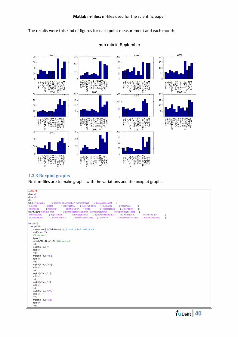
Matlab m-files: m-files used for the scientific paper

40

The results were this kind of figures for each point measurement and each month:

1.3.3 Boxplot graphs

Next m-files are to make graphs with the variations and the boxplot graphs.

m-file 23 clear all; close all; clc; tekst=['Nilebasin ' ; 'albertnilebahraljabal'; 'bahrelghazal '; 'baroakobosobat '; 'bluenile '; 'kagera '; 'lakevictoria '; 'lowerwhitenile '; 'mainnile1 '; 'mainnile2 ' ; 'mainnile3 '; 'mainnile4 '; 'semlikilalbert '; 'sudd '; 'tekezzeatbara '; 'victorianile ']; teksttwee=['Nilebasin.mat ' ; 'albertnilebahraljabal.mat'; 'bahrelghazal.mat '; 'baroakobosobat.mat '; 'bluenile.mat '; 'kagera.mat '; 'lakevictoria.mat '; 'lowerwhitenile.mat '; 'mainnile1.mat '; 'mainnile2.mat ' ; 'mainnile3.mat '; 'mainnile4.mat '; 'semlikilalbert.mat '; 'sudd.mat '; 'tekezzeatbara.mat '; 'victorianile.mat ']; for t=1:16 for y=0:10 open=sprintf('%s',teksttwee(t,:)); % result m-file 21 with bicubic load(open, 'T'); %% plot dots figure (t) x=[1+(y*12):12+(y*12)]; %time period r=1; h=plot(x,T(r,x),'.'); hold on r=2; h=plot(x,T(r,x),'yo'); hold on r=3; h=plot(x,T(r,x),'m+'); hold on r=4; h=plot(x,T(r,x),'cx'); hold on r=5; h=plot(x,T(r,x),'rv'); hold on r=6; h=plot(x,T(r,x),'g^'); hold on r=7; h=plot(x,T(r,x),'ks'); hold on r=8;

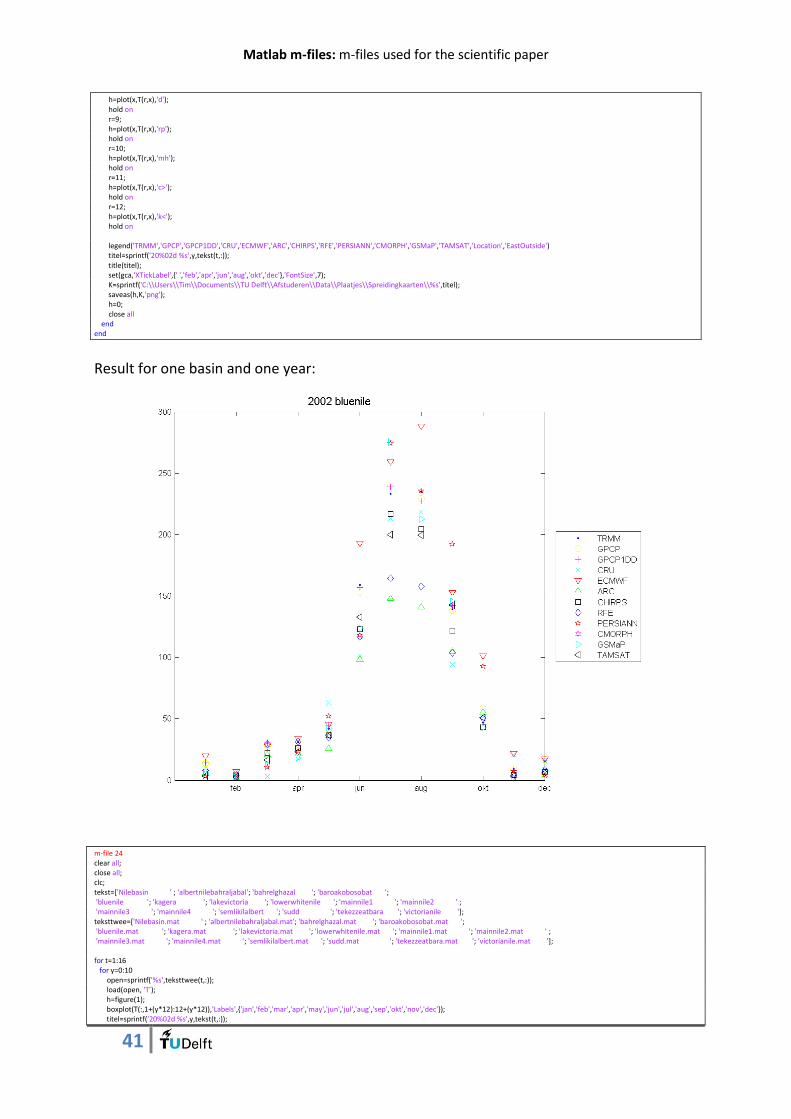
Matlab m-files: m-files used for the scientific paper

41

h=plot(x,T(r,x),'d'); hold on r=9; h=plot(x,T(r,x),'rp'); hold on r=10; h=plot(x,T(r,x),'mh'); hold on r=11; h=plot(x,T(r,x),'c>'); hold on r=12; h=plot(x,T(r,x),'k<'); hold on legend('TRMM','GPCP','GPCP1DD','CRU','ECMWF','ARC','CHIRPS','RFE','PERSIANN','CMORPH','GSMaP','TAMSAT','Location','EastOutside') titel=sprintf('20%02d %s',y,tekst(t,:)); title(titel); set(gca,'XTickLabel',{' ','feb','apr','jun','aug','okt','dec'},'FontSize',7); K=sprintf('C:\\Users\\Tim\\Documents\\TU Delft\\Afstuderen\\Data\\Plaatjes\\Spreidingkaarten\\%s',titel); saveas(h,K,'png'); h=0; close all end end

Result for one basin and one year:

m-file 24 clear all; close all; clc; tekst=['Nilebasin ' ; 'albertnilebahraljabal'; 'bahrelghazal '; 'baroakobosobat '; 'bluenile '; 'kagera '; 'lakevictoria '; 'lowerwhitenile '; 'mainnile1 '; 'mainnile2 ' ; 'mainnile3 '; 'mainnile4 '; 'semlikilalbert '; 'sudd '; 'tekezzeatbara '; 'victorianile ']; teksttwee=['Nilebasin.mat ' ; 'albertnilebahraljabal.mat'; 'bahrelghazal.mat '; 'baroakobosobat.mat '; 'bluenile.mat '; 'kagera.mat '; 'lakevictoria.mat '; 'lowerwhitenile.mat '; 'mainnile1.mat '; 'mainnile2.mat ' ; 'mainnile3.mat '; 'mainnile4.mat '; 'semlikilalbert.mat '; 'sudd.mat '; 'tekezzeatbara.mat '; 'victorianile.mat ']; for t=1:16 for y=0:10 open=sprintf('%s',teksttwee(t,:)); load(open, 'T'); h=figure(1); boxplot(T(:,1+(y*12):12+(y*12)),'Labels',{'jan','feb','mar','apr','may','jun','jul','aug','sep','okt','nov','dec'}); titel=sprintf('20%02d %s',y,tekst(t,:));

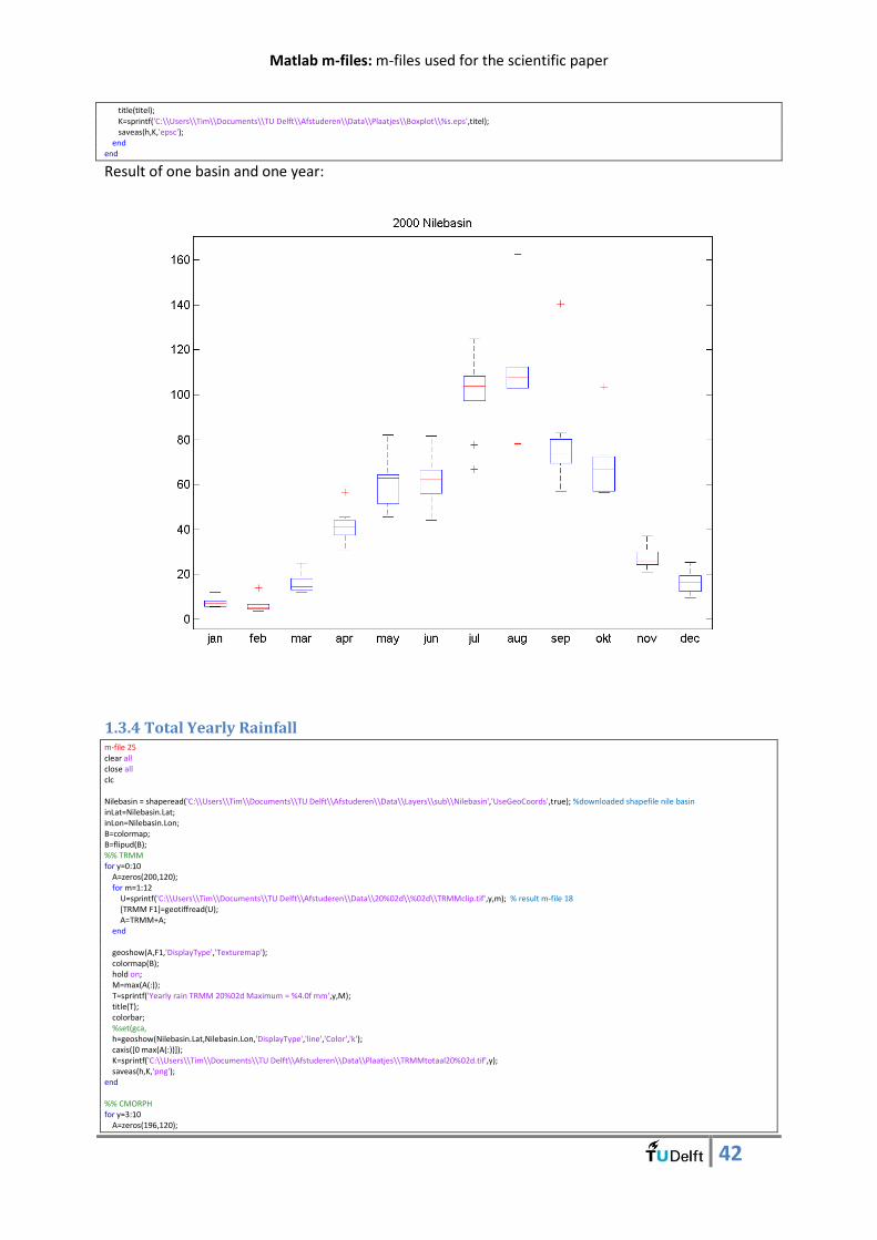
Matlab m-files: m-files used for the scientific paper

42

title(titel); K=sprintf('C:\\Users\\Tim\\Documents\\TU Delft\\Afstuderen\\Data\\Plaatjes\\Boxplot\\%s.eps',titel); saveas(h,K,'epsc'); end end

Result of one basin and one year:

1.3.4 Total Yearly Rainfall m-file 25 clear all close all clc Nilebasin = shaperead('C:\\Users\\Tim\\Documents\\TU Delft\\Afstuderen\\Data\\Layers\\sub\\Nilebasin','UseGeoCoords',true); %downloaded shapefile nile basin inLat=Nilebasin.Lat; inLon=Nilebasin.Lon; B=colormap; B=flipud(B); %% TRMM for y=0:10 A=zeros(200,120); for m=1:12 U=sprintf('C:\\Users\\Tim\\Documents\\TU Delft\\Afstuderen\\Data\\20%02d\\%02d\\TRMMclip.tif',y,m); % result m-file 18 [TRMM F1]=geotiffread(U); A=TRMM+A; end geoshow(A,F1,'DisplayType','Texturemap'); colormap(B); hold on; M=max(A(:)); T=sprintf('Yearly rain TRMM 20%02d Maximum = %4.0f mm',y,M); title(T); colorbar; %set(gca, h=geoshow(Nilebasin.Lat,Nilebasin.Lon,'DisplayType','line','Color','k'); caxis([0 max(A(:))]); K=sprintf('C:\\Users\\Tim\\Documents\\TU Delft\\Afstuderen\\Data\\Plaatjes\\TRMMtotaal20%02d.tif',y); saveas(h,K,'png'); end %% CMORPH for y=3:10 A=zeros(196,120);

Matlab m-files: m-files used for the scientific paper

43

for m=1:12 U=sprintf('C:\\Users\\Tim\\Documents\\TU Delft\\Afstuderen\\Data\\20%02d\\%02d\\CMORPHclip.tif',y,m); % result m-file 18 [CMORPH F1]=geotiffread(U); A=CMORPH+A; end geoshow(A,F1,'DisplayType','Texturemap'); colormap(B); hold on; M=max(A(:)); T=sprintf('Yearly rain CMORPH 20%02d Maximum = %4.0f mm',y,M); title(T); axis([20 50 -10 39]); colorbar; %set(gca, h=geoshow(Nilebasin.Lat,Nilebasin.Lon,'DisplayType','line','Color','k'); caxis([0 max(A(:))]); K=sprintf('C:\\Users\\Tim\\Documents\\TU Delft\\Afstuderen\\Data\\Plaatjes\\CMORPHtotaal20%02d.tif',y); saveas(h,K,'png'); end %% RFE for y=1:10 A=zeros(501,301); for m=1:12 U=sprintf('C:\\Users\\Tim\\Documents\\TU Delft\\Afstuderen\\Data\\20%02d\\%02d\\FEWSNETclip.tif',y,m); % result m-file 18 [RFE F1]=geotiffread(U); for q=1:501 for w=1:301 if (RFE(q,w))<0; RFE(q,w)=0; end end end A=RFE+A; end geoshow(A,F1,'DisplayType','Texturemap'); colormap(B); hold on; M=max(A(:)); T=sprintf('Yearly rain RFE 20%02d Maximum = %4.0f mm',y,M); title(T); colorbar; axis([20 50 -10 40]); h=geoshow(Nilebasin.Lat,Nilebasin.Lon,'DisplayType','line','Color','k'); caxis([0 max(A(:))]); K=sprintf('C:\\Users\\Tim\\Documents\\TU Delft\\Afstuderen\\Data\\Plaatjes\\RFEtotaal20%02d.tif',y); saveas(h,K,'png'); end %% ARC for y=0:10 A=zeros(501,301); for m=1:12 U=sprintf('C:\\Users\\Tim\\Documents\\TU Delft\\Afstuderen\\Data\\20%02d\\%02d\\ARCclip.tif',y,m); % result m-file 18 [ARC F1]=geotiffread(U); for q=1:501 for w=1:301 if (ARC(q,w))<0; ARC(q,w)=0; end end end A=ARC+A; end geoshow(A,F1,'DisplayType','Texturemap'); colormap(B); hold on; M=max(A(:)); T=sprintf('Yearly rain ARC 20%02d Maximum = %4.0f mm',y,M); title(T); colorbar; axis([20 50 -10 40]); h=geoshow(Nilebasin.Lat,Nilebasin.Lon,'DisplayType','line','Color','k'); caxis([0 max(A(:))]); K=sprintf('C:\\Users\\Tim\\Documents\\TU Delft\\Afstuderen\\Data\\Plaatjes\\ARCtotaal20%02d.tif',y); saveas(h,K,'png'); end %% GPCP for y=0:10 A=zeros(20,12); for m=1:12 U=sprintf('C:\\Users\\Tim\\Documents\\TU Delft\\Afstuderen\\Data\\20%02d\\%02d\\GPCPclip.tif',y,m); % result m-file 18 [GPCP F1]=geotiffread(U); for q=1:20 for w=1:12 if (GPCP(q,w))<0; GPCP(q,w)=0;

Matlab m-files: m-files used for the scientific paper

44

end end end A=GPCP+A; end geoshow(A,F1,'DisplayType','Texturemap'); colormap(B); hold on; M=max(A(:)); T=sprintf('Yearly rain GPCP 20%02d Maximum = %4.0f mm',y,M); title(T); colorbar; axis([20 50 -10 40]); h=geoshow(Nilebasin.Lat,Nilebasin.Lon,'DisplayType','line','Color','k'); caxis([0 max(A(:))]); K=sprintf('C:\\Users\\Tim\\Documents\\TU Delft\\Afstuderen\\Data\\Plaatjes\\GPCPtotaal20%02d.tif',y); saveas(h,K,'png'); end %% GPCP1dd for y=0:10 A=zeros(50,30); for m=1:12 U=sprintf('C:\\Users\\Tim\\Documents\\TU Delft\\Afstuderen\\Data\\20%02d\\%02d\\GPCP1DDclip.tif',y,m); % result m-file 18 [GPCP F1]=geotiffread(U); for q=1:50 for w=1:30 if (GPCP(q,w))<0; GPCP(q,w)=0; end end end A=GPCP+A; end geoshow(A,F1,'DisplayType','Texturemap'); colormap(B); hold on; M=max(A(:)); T=sprintf('Yearly rain GPCP1DD 20%02d Maximum = %4.0f mm',y,M); title(T); colorbar; axis([20 50 -10 40]); h=geoshow(Nilebasin.Lat,Nilebasin.Lon,'DisplayType','line','Color','k'); caxis([0 max(A(:))]); K=sprintf('C:\\Users\\Tim\\Documents\\TU Delft\\Afstuderen\\Data\\Plaatjes\\GPCP1DDtotaal20%02d.tif',y); saveas(h,K,'png'); end %% CHIRPS for y=0:10 A=zeros(1000,600); for m=1:12 U=sprintf('C:\\Users\\Tim\\Documents\\TU Delft\\Afstuderen\\Data\\20%02d\\%02d\\CHIRPSclip.tif',y,m); % result m-file 18 [CHIRPS F1]=geotiffread(U); for q=1:1000 for w=1:600 if (CHIRPS(q,w))<0; CHIRPS(q,w)=0; end end end for q=1:1000 for w=1:600 if isnan(CHIRPS(q,w)); CHIRPS(q,w)=0; end end end A=CHIRPS+A; end geoshow(A,F1,'DisplayType','Texturemap'); colormap(B); hold on; M=max(A(:)); T=sprintf('Yearly rain CHIRPS 20%02d Maximum = %4.0f mm',y,M); title(T); colorbar; axis([20 50 -10 40]); h=geoshow(Nilebasin.Lat,Nilebasin.Lon,'DisplayType','line','Color','k'); caxis([0 max(A(:))]); K=sprintf('C:\\Users\\Tim\\Documents\\TU Delft\\Afstuderen\\Data\\Plaatjes\\CHIRPStotaal20%02d.tif',y); saveas(h,K,'png'); end %% GPCP for y=0:10 A=zeros(20,12); for m=1:12 U=sprintf('C:\\Users\\Tim\\Documents\\TU Delft\\Afstuderen\\Data\\20%02d\\%02d\\GPCPclip.tif',y,m); % result m-file 18 [GPCP F1]=geotiffread(U);

Matlab m-files: m-files used for the scientific paper

45

for q=1:20 for w=1:12 if (GPCP(q,w))<0; GPCP(q,w)=0; end end end A=GPCP+A; end geoshow(A,F1,'DisplayType','Texturemap'); colormap(B); hold on; M=max(A(:)); T=sprintf('Yearly rain GPCP 20%02d Maximum = %4.0f mm',y,M); title(T); colorbar; axis([20 50 -10 40]); h=geoshow(Nilebasin.Lat,Nilebasin.Lon,'DisplayType','line','Color','k'); caxis([0 max(A(:))]); K=sprintf('C:\\Users\\Tim\\Documents\\TU Delft\\Afstuderen\\Data\\Plaatjes\\GPCPtotaal20%02d.tif',y); saveas(h,K,'png'); end %% CRU for y=0:10 A=zeros(100,60); for m=1:12 U=sprintf('C:\\Users\\Tim\\Documents\\TU Delft\\Afstuderen\\Data\\20%02d\\%02d\\CRUclip.tif',y,m); % result m-file 18 [CRU F1]=geotiffread(U); for q=1:100 for w=1:60 if (CRU(q,w))<0; CRU(q,w)=0; end end end A=CRU+A; end geoshow(A,F1,'DisplayType','Texturemap'); colormap(B); hold on; M=max(A(:)); T=sprintf('Yearly rain CRU 20%02d Maximum = %4.0f mm',y,M); title(T); colorbar; axis([20 50 -10 40]); h=geoshow(Nilebasin.Lat,Nilebasin.Lon,'DisplayType','line','Color','k'); caxis([0 max(A(:))]); K=sprintf('C:\\Users\\Tim\\Documents\\TU Delft\\Afstuderen\\Data\\Plaatjes\\CRUtotaal20%02d.tif',y); saveas(h,K,'png'); end %% ECMWF for y=0:10 A=zeros(66,41); for m=1:12 U=sprintf('C:\\Users\\Tim\\Documents\\TU Delft\\Afstuderen\\Data\\20%02d\\%02d\\ECMWFclip.tif',y,m); % result m-file 18 [ECMWF F1]=geotiffread(U); for q=1:66 for w=1:41 if (ECMWF(q,w))<0; ECMWF(q,w)=0; end end end A=ECMWF+A; end geoshow(A,F1,'DisplayType','Texturemap'); colormap(B); hold on; M=max(A(:)); T=sprintf('Yearly rain ECMWF 20%02d Maximum = %4.0f mm',y,M); title(T); colorbar; axis([20 50 -10 38]); h=geoshow(Nilebasin.Lat,Nilebasin.Lon,'DisplayType','line','Color','k'); caxis([0 max(A(:))]); K=sprintf('C:\\Users\\Tim\\Documents\\TU Delft\\Afstuderen\\Data\\Plaatjes\\ECMWFtotaal20%02d.tif',y); saveas(h,K,'png'); end %% TAMSAT for y=0:5 A=zeros(1287,809); for m=1:12 U=sprintf('C:\\Users\\Tim\\Documents\\TU Delft\\Afstuderen\\Data\\20%02d\\%02d\\TAMSATclip.tif',y,m); % result m-file 18 [TAMSAT F1]=geotiffread(U); for q=1:1287

Matlab m-files: m-files used for the scientific paper

46

for w=1:809 if (TAMSAT(q,w))<0; TAMSAT(q,w)=0; end end end A=TAMSAT+A; end geoshow(A,F1,'DisplayType','Texturemap'); colormap(B); hold on; M=max(A(:)); T=sprintf('Yearly rain TAMSAT 20%02d Maximum = %4.0f mm',y,M); title(T); colorbar; axis([20 50 -10 38]); h=geoshow(Nilebasin.Lat,Nilebasin.Lon,'DisplayType','line','Color','k'); caxis([0 max(A(:))]); K=sprintf('C:\\Users\\Tim\\Documents\\TU Delft\\Afstuderen\\Data\\Plaatjes\\TAMSATtotaal20%02d.tif',y); saveas(h,K,'png'); end for y=7:10 A=zeros(1287,809); for m=1:12 U=sprintf('C:\\Users\\Tim\\Documents\\TU Delft\\Afstuderen\\Data\\20%02d\\%02d\\TAMSATclip.tif',y,m); % result m-file 18 [TAMSAT F1]=geotiffread(U); for q=1:1287 for w=1:809 if (TAMSAT(q,w))<0; TAMSAT(q,w)=0; end end end A=TAMSAT+A; end geoshow(A,F1,'DisplayType','Texturemap'); colormap(B); hold on; M=max(A(:)); T=sprintf('Yearly rain TAMSAT 20%02d Maximum = %4.0f mm',y,M); title(T); colorbar; axis([20 50 -10 38]); h=geoshow(Nilebasin.Lat,Nilebasin.Lon,'DisplayType','line','Color','k'); caxis([0 max(A(:))]); K=sprintf('C:\\Users\\Tim\\Documents\\TU Delft\\Afstuderen\\Data\\Plaatjes\\TAMSATtotaal20%02d.tif',y); saveas(h,K,'png'); end %% GSMaP for y=2:9 A=zeros(500,300); for m=1:12 U=sprintf('C:\\Users\\Tim\\Documents\\TU Delft\\Afstuderen\\Data\\20%02d\\%02d\\GSMaPclip.tif',y,m); % result m-file 18 [GSMaP F1]=geotiffread(U); for q=1:500 for w=1:300 if (GSMaP(q,w))<0; GSMaP(q,w)=0; end end end A=GSMaP+A; end geoshow(A,F1,'DisplayType','Texturemap'); colormap(B); hold on; M=max(A(:)); T=sprintf('Yearly rain GSMaP 20%02d Maximum = %4.0f mm',y,M); title(T); colorbar; axis([20 50 -10 40]); h=geoshow(Nilebasin.Lat,Nilebasin.Lon,'DisplayType','line','Color','k'); caxis([0 max(A(:))]); K=sprintf('C:\\Users\\Tim\\Documents\\TU Delft\\Afstuderen\\Data\\Plaatjes\\GSMaPtotaal20%02d.tif',y); saveas(h,K,'png'); end %% PERSIANN for y=1:10 A=zeros(200,120); for m=1:12 U=sprintf('C:\\Users\\Tim\\Documents\\TU Delft\\Afstuderen\\Data\\20%02d\\%02d\\PERSIANNclip.tif',y,m); % result m-file 18 [PERSIANN F1]=geotiffread(U); for q=1:200 for w=1:120 if (PERSIANN(q,w))<0; PERSIANN(q,w)=0;

Matlab m-files: m-files used for the scientific paper

47

end end end A=PERSIANN+A; end geoshow(A,F1,'DisplayType','Texturemap'); colormap(B); hold on; M=max(A(:)); T=sprintf('Yearly rain PERSIANN 20%02d Maximum = %4.0f mm',y,M); title(T); colorbar; axis([20 50 -10 40]); h=geoshow(Nilebasin.Lat,Nilebasin.Lon,'DisplayType','line','Color','k'); caxis([0 max(A(:))]); K=sprintf('C:\\Users\\Tim\\Documents\\TU Delft\\Afstuderen\\Data\\Plaatjes\\PERSIANNtotaal20%02d.tif',y); saveas(h,K,'png'); end

Results are annual rainfall maps of all the products for every year. And also the maximum measured

rainfall is shown.

Matlab m-files: m-files used for the scientific paper

48

2. Ground Measurements The ground measurements have each an excel file which has the same structure. Those excel file are

collected by matlab and all those measurements are also saved in a .mat file called

metingenmat.mat. Sometimes, the .mat file is opened by matlab, this is done when enough memory

is available. This makes the m-file quicker. But when not enough memory is available, matlab opens

the .xls files one by one. The metingenmat.mat is for the monthly rainfall values and the

metingenmatjaar.mat is for the yearly rainfall values. They are made as follows:

Monthly:

m-file 26 clear all; close all; clc; %% eerst map maken met alle metingen. tekst=['sennar ' ; 'rashad ' ; 'obied ' ; 'nyala ' ; 'nahoud ' ; 'madani ' ; 'kosti ' ; 'khar ' ; 'kasala ' ; 'kadugli ' ; 'atbara ' ; 'gadarf ' ; 'fasher ' ; 'duem ' ; 'damazine ' ; 'babanusa '; 'gondor ';'asswan '; 'cairo ';'luxor ';'qena ';'asyout ';'elminya ';'dangla ';'debretabor ';'addiszemen ';'ayikel '; 'adet ';'gorgora ';'enjibara ';'enfraz ';'wereta ';'zege ';'maksegnit ';'kidmaja ';'kimbaba ';'wetetabay ';'gundil ';'abayshelek ';'urana ';'wau ';'malakal ';'juba ';'yetemen ';'shindi ';'debremarcos';'teppi ';'masha ';'assosa ';'begi ';'sekela ';'motta ';'finote ';'gebeya ';'kitale ';'eldoret ';'kisumu ';'bukoba ';'musoma ';'mwanza ';'kigoma ';'kigali ']; teksttwee=['SENNAR.xls ' ; 'RASHAD.xls ' ; 'OBIED.xls ' ; 'NYALA.xls ' ; 'NAHOUD.xls ' ; 'MADANI.xls ' ; 'kosti.xls ' ; 'KHAR_RAIN.xls ' ; 'KASALA.xls ' ; 'KADUGLI.xls ' ; 'ATBARA.xls ' ; 'GADARF.xls ' ; 'FASHER.xls ' ; 'DUEM.xls ' ; 'DAMAZINE.xls ' ; 'BABANUSARAIN.xls'; 'GONDOR.xlsx '; 'ASSWAN.xlsx '; 'CAIRO.xlsx '; 'LUXOR.xlsx '; 'QENA.xlsx '; 'ASYOUT.xlsx '; 'ELMINYA.xlsx ';'DANGLA.xlsx '; 'DEBRETABOR.xlsx '; 'ADDISZEMEN.xlsx '; 'AYIKEL.xlsx '; 'ADET.xlsx '; 'GORGORA.xlsx ';'ENJIBARA.xlsx ';'ENFRAZ.xlsx '; 'WERETA.xlsx '; 'ZEGE.xlsx '; 'MAKSEGNIT.xlsx '; 'KIDMAJA.xlsx '; 'KIMBABA.xlsx '; 'WETETABAY.xlsx '; 'GUNDIL.xlsx '; 'ABAYSHELEKO.xlsx'; 'URANA.xlsx ';'WAU.xlsx ';'MALAKAL.xlsx ';'JUBA.xlsx '; 'YETEMEN.xlsx ';'SHINDI.xlsx ';'DEBREMARCOS.xlsx';'TEPPI.xlsx ';'MASHA.xlsx ';'ASSOSA.xlsx ';'BEGI.xlsx ';'SEKELA.xlsx ';'MOTTA.xlsx ';'FINOTE.xlsx ';'GEBEYA.xlsx ';'KITALE.xlsx ';'ELDORET.xlsx ';'KISUMU.xlsx ';'BUKOBA.xlsx ';'MUSOMA.xlsx ';'MWANZA.xlsx ';'KIGOMA.xlsx ';'KIGALI.xlsx ' ]; for v=1:62; open=sprintf('C:\\Users\\Tim\\Documents\\TU Delft\\Afstuderen\\Rainfall data ground\\%s',teksttwee(v,:)); % downloaded and organized ground measurements A=xlsread(open); B=A(1:11,2:13); B=B'; C=reshape(B,1,132); C=C'; P(:,v)=C(:); C=0; end grond=P; save('Metingenmat','grond');

Yearly:

m-file 27 clear all; close all; clc; % eerst map maken met alle metingen. tekst=['sennar ' ; 'rashad ' ; 'obied ' ; 'nyala ' ; 'nahoud ' ; 'madani ' ; 'kosti ' ; 'khar ' ; 'kasala ' ; 'kadugli ' ; 'atbara ' ; 'gadarf ' ; 'fasher ' ; 'duem ' ; 'damazine ' ; 'babanusa '; 'gondor ';'asswan '; 'cairo ';'luxor ';'qena ';'asyout ';'elminya ';'dangla ';'debretabor ';'addiszemen ';'ayikel '; 'adet ';'gorgora ';'enjibara ';'enfraz ';'wereta ';'zege ';'maksegnit ';'kidmaja ';'kimbaba ';'wetetabay ';'gundil ';'abayshelek ';'urana ';'wau ';'malakal ';'juba ';'yetemen ';'shindi ';'debremarcos';'teppi ';'masha ';'assosa ';'begi ';'sekela ';'motta ';'finote ';'gebeya ';'kitale ';'eldoret ';'kisumu ';'bukoba ';'musoma ';'mwanza ';'kigoma ';'kigali ']; teksttwee=['SENNAR.xls ' ; 'RASHAD.xls ' ; 'OBIED.xls ' ; 'NYALA.xls ' ; 'NAHOUD.xls ' ; 'MADANI.xls ' ; 'kosti.xls ' ; 'KHAR_RAIN.xls ' ; 'KASALA.xls ' ; 'KADUGLI.xls ' ; 'ATBARA.xls ' ; 'GADARF.xls ' ; 'FASHER.xls ' ; 'DUEM.xls ' ; 'DAMAZINE.xls ' ; 'BABANUSARAIN.xls'; 'GONDOR.xlsx '; 'ASSWAN.xlsx '; 'CAIRO.xlsx '; 'LUXOR.xlsx '; 'QENA.xlsx '; 'ASYOUT.xlsx '; 'ELMINYA.xlsx ';'DANGLA.xlsx '; 'DEBRETABOR.xlsx '; 'ADDISZEMEN.xlsx '; 'AYIKEL.xlsx '; 'ADET.xlsx '; 'GORGORA.xlsx ';'ENJIBARA.xlsx ';'ENFRAZ.xlsx '; 'WERETA.xlsx '; 'ZEGE.xlsx '; 'MAKSEGNIT.xlsx '; 'KIDMAJA.xlsx '; 'KIMBABA.xlsx '; 'WETETABAY.xlsx '; 'GUNDIL.xlsx '; 'ABAYSHELEKO.xlsx'; 'URANA.xlsx ';'WAU.xlsx ';'MALAKAL.xlsx ';'JUBA.xlsx '; 'YETEMEN.xlsx ';'SHINDI.xlsx ';'DEBREMARCOS.xlsx';'TEPPI.xlsx ';'MASHA.xlsx ';'ASSOSA.xlsx ';'BEGI.xlsx ';'SEKELA.xlsx ';'MOTTA.xlsx ';'FINOTE.xlsx ';'GEBEYA.xlsx ';'KITALE.xlsx ';'ELDORET.xlsx ';'KISUMU.xlsx ';'BUKOBA.xlsx ';'MUSOMA.xlsx ';'MWANZA.xlsx ';'KIGOMA.xlsx ';'KIGALI.xlsx ' ]; for v=1:62; open=sprintf('C:\\Users\\Tim\\Documents\\TU Delft\\Afstuderen\\Rainfall data ground\\%s',teksttwee(v,:)); % downloaded and organized ground measurements A=xlsread(open); B=A(1:11,2:13); B=B'; C=reshape(B,1,132); C=C'; P(:,v)=C(:); C=0; end grond=P; save('Metingenmatjaar','grond');

Here a map is made which shows the location of the ground measurements:

m-file 28 clear all; close all;

Matlab m-files: m-files used for the scientific paper

49

clc; %% map limits latlim = [35 -10]; lonlim = [20 45]; %% plot empty map axesm('mercator','grid','on','MapLatLimit',latlim,'MapLonLimit',lonlim); tightmap; framem on; mlabel on; plabel on; set(gca,'Color',[0.8 0.8 0.8]); setm(gca,'PLineLocation',10,'PlabelLocation',10,'MLineLocation',10,'MlabelLocation',10); %% load shapefiles Eritrea = shaperead('Layers\ERI_adm0','UseGeoCoords',true); % downloaded Sudan = shaperead('Layers\SDN_adm0','UseGeoCoords',true); Southsudan = shaperead('Layers\SSD_adm0','UseGeoCoords',true); Chad = shaperead('Layers\TCD_adm0','UseGeoCoords',true); Centralafrica = shaperead('Layers\CAF_adm0','UseGeoCoords',true); Democraticcongo = shaperead('Layers\COD_adm0','UseGeoCoords',true); Rwanda = shaperead('Layers\RWA_adm0','UseGeoCoords',true); Kenya = shaperead('Layers\KEN_adm0','UseGeoCoords',true); Burundi = shaperead('Layers\BDI_adm0','UseGeoCoords',true); Uganda = shaperead('Layers\UGA_adm0','UseGeoCoords',true); Tanzania = shaperead('Layers\TZA_adm0','UseGeoCoords',true); Libya = shaperead('Layers\LBY_adm0','UseGeoCoords',true); Israel = shaperead('Layers\ISR_adm0','UseGeoCoords',true); Ethiopia = shaperead('Layers\ETH_adm0','UseGeoCoords',true); Egypt = shaperead('Layers\EGY_adm0','UseGeoCoords',true); Jordan = shaperead('Layers\JOR_adm0','UseGeoCoords',true); Saudi = shaperead('Layers\SAU_adm0','UseGeoCoords',true); Yemen = shaperead('Layers\YEM_adm0','UseGeoCoords',true); Nilebasin = shaperead('Layers\Sub\Nilebasin','UseGeoCoords',true); Rivers = shaperead('Layers\ne_10m_rivers_lake_centerlines','UseGeoCoords',true); %% point ground measurements [Meting(1:62).Geometry]=deal('Point'); Meting(1).Lat=13.55; Meting(1).Lon=33.617; Meting(1).Name='Sennar'; Meting(2).Lat=11.87; Meting(2).Lon=31.05; Meting(2).Name='Rashad'; Meting(3).Lat=13.167; Meting(3).Lon=30.233; Meting(3).Name='Obied'; Meting(4).Lat=12.05; Meting(4).Lon=24.883; Meting(4).Name='Nyala'; Meting(5).Lat=12.7; Meting(5).Lon=28.433; Meting(5).Name='Nahoud'; Meting(6).Lat=14.4; Meting(6).Lon=33.48; Meting(6).Name='Madini'; Meting(7).Lat=13.17; Meting(7).Lon=32.67; Meting(7).Name='Kosti'; Meting(8).Lat=15.6; Meting(8).Lon=32.549; Meting(8).Name='Khar'; Meting(9).Lat=15.467; Meting(9).Lon=36.4; Meting(9).Name='Kasala'; Meting(10).Lat=11; Meting(10).Lon=29.72; Meting(10).Name='Kadugli'; Meting(11).Lat=17.7; Meting(11).Lon=33.97; Meting(11).Name='Atbara'; Meting(12).Lat=14.033; Meting(12).Lon=35.4; Meting(12).Name='Gadarf'; Meting(13).Lat=13.617; Meting(13).Lon=25.333; Meting(13).Name='Fasher'; Meting(14).Lat=13.98; Meting(14).Lon=32.33; Meting(14).Name='Duem'; Meting(15).Lat=11.78; Meting(15).Lon=34.38; Meting(15).Name='Damazine'; Meting(16).Lat=11.333; Meting(16).Lon=27.817; Meting(16).Name='Babanusa'; Meting(17).Lat=12.550; Meting(17).Lon=37.417; Meting(17).Name='Gondor'; Meting(18).Lat=23.966; Meting(18).Lon=32.783; Meting(18).Name='Asswan'; Meting(19).Lat=30.31; Meting(19).Lon=31.04; Meting(19).Name='Cairo'; Meting(20).Lat=25.67; Meting(20).Lon=32.7; Meting(20).Name='Luxor'; Meting(21).Lat=26.2; Meting(21).Lon=32.75; Meting(21).Name='Qena'; Meting(22).Lat=27.18; Meting(22).Lon=31.3; Meting(22).Name='Asyout'; Meting(23).Lat=28.08; Meting(23).Lon=30.73; Meting(23).Name='Elminya'; Meting(24).Lat=11.117; Meting(24).Lon=36.417; Meting(24).Name='Dangla'; Meting(25).Lat=11.883; Meting(25).Lon=38.033; Meting(25).Name='Debretabor'; Meting(26).Lat=12.117; Meting(26).Lon=37.867; Meting(26).Name='Addiszemen'; Meting(27).Lat=12.533; Meting(27).Lon=37.050; Meting(27).Name='Ayikel'; Meting(28).Lat=11.267; Meting(28).Lon=37.467; Meting(28).Name='Adet'; Meting(29).Lat=12.250; Meting(29).Lon=37.300; Meting(29).Name='Gorgora'; Meting(30).Lat=11.000; Meting(30).Lon=37.000; Meting(30).Name='Enjibara'; Meting(31).Lat=12.183; Meting(31).Lon=37.683; Meting(31).Name='Enfraz'; Meting(32).Lat=11.917; Meting(32).Lon=37.683; Meting(32).Name='Wereta'; Meting(33).Lat=11.683; Meting(33).Lon=37.317; Meting(33).Name='Zege'; Meting(34).Lat=12.367; Meting(34).Lon=37.550; Meting(34).Name='Maksegnit'; Meting(35).Lat=11.000; Meting(35).Lon=36.800; Meting(35).Name='Kidmaja'; Meting(36).Lat=11.550; Meting(36).Lon=37.380; Meting(36).Name='Kimbaba'; Meting(37).Lat=11.367; Meting(37).Lon=37.050; Meting(37).Name='Wetetabay'; Meting(38).Lat=10.950; Meting(38).Lon=37.070; Meting(38).Name='Gundil'; Meting(39).Lat=11.383; Meting(39).Lon=36.870; Meting(39).Name='AbaySheleko'; Meting(40).Lat=10.892; Meting(40).Lon=36.856; Meting(40).Name='Urana'; Meting(41).Lat=7.42; Meting(41).Lon=28.01; Meting(41).Name='Wau'; Meting(42).Lat=9.33; Meting(42).Lon=31.39; Meting(42).Name='Malakal'; Meting(43).Lat=4.52; Meting(43).Lon=31.36; Meting(43).Name='Juba'; Meting(44).Lat=10.33; Meting(44).Lon=38.13; Meting(44).Name='Yetemen'; Meting(45).Lat=10.43; Meting(45).Lon=36.57; Meting(45).Name='Shindi'; Meting(46).Lat=10.21; Meting(46).Lon=37.43; Meting(46).Name='Debremarcos'; Meting(47).Lat=7.2; Meting(47).Lon=35.42; Meting(47).Name='Teppi'; Meting(48).Lat=7.73; Meting(48).Lon=35.48; Meting(48).Name='Masha'; Meting(49).Lat=10.02; Meting(49).Lon=34.32; Meting(49).Name='Assosa'; Meting(50).Lat=9.35; Meting(50).Lon=34.53; Meting(50).Name='Begi'; Meting(51).Lat=11; Meting(51).Lon=37.13; Meting(51).Name='Sekela'; Meting(52).Lat=11.083; Meting(52).Lon=37.867; Meting(52).Name='Motta'; Meting(53).Lat=10.41; Meting(53).Lon=37.16; Meting(53).Name='Finote'; Meting(54).Lat=9.2; Meting(54).Lon=39.38; Meting(54).Name='Gebeya'; Meting(55).Lat=1.016; Meting(55).Lon=35; Meting(55).Name='Kitale'; Meting(56).Lat=0.405; Meting(56).Lon=35.224; Meting(56).Name='Eldoret'; Meting(57).Lat=-0.1; Meting(57).Lon=34.75; Meting(57).Name='Kisumu';

Matlab m-files: m-files used for the scientific paper

50

Meting(58).Lat=-1.333; Meting(58).Lon=31.817; Meting(58).Name='Bukoba'; Meting(59).Lat=-1.5; Meting(59).Lon=33.8; Meting(59).Name='Musoma'; Meting(60).Lat=-2.467; Meting(60).Lon=32.917; Meting(60).Name='Mwanza'; Meting(61).Lat=-4.88; Meting(61).Lon=29.63; Meting(61).Name='Kigoma'; Meting(62).Lat=-1.96; Meting(62).Lon=30.13; Meting(62).Name='Kigali'; %% put on or off the shapefiles Eritrea.plot = 1; Sudan.plot = 1; Southsudan.plot = 1; Chad.plot = 1; Centralafrica.plot = 1; Democraticcongo.plot = 1; Rwanda.plot = 1; Kenya.plot = 1; Burundi.plot = 1; Uganda.plot = 1; Tanzania.plot = 1; Libya.plot = 1; Israel.plot = 1; Ethiopia.plot = 1; Egypt.plot = 1; Jordan.plot = 1; Saudi.plot = 1; Yemen.plot = 1; Nilebasin.plot = 1; if(Eritrea.plot == 1); geoshow(Eritrea.Lat,Eritrea.Lon,'DisplayType','line','Color','k') end if(Sudan.plot == 1); geoshow(Sudan.Lat,Sudan.Lon,'DisplayType','line','Color','k') end if(Southsudan.plot == 1); geoshow(Southsudan.Lat,Southsudan.Lon,'DisplayType','line','Color','k') end if(Chad.plot == 1); geoshow(Chad.Lat,Chad.Lon,'DisplayType','line','Color','k') end if(Centralafrica.plot == 1); geoshow(Centralafrica.Lat,Centralafrica.Lon,'DisplayType','line','Color','k') end if(Democraticcongo.plot == 1); geoshow(Democraticcongo.Lat,Democraticcongo.Lon,'DisplayType','line','Color','k') end if(Kenya.plot == 1); geoshow(Kenya.Lat,Kenya.Lon,'DisplayType','line','Color','k') end if(Burundi.plot == 1); geoshow(Burundi.Lat,Burundi.Lon,'DisplayType','line','Color','k') end if(Uganda.plot == 1); geoshow(Uganda.Lat,Uganda.Lon,'DisplayType','line','Color','k') end if(Tanzania.plot == 1); geoshow(Tanzania.Lat,Tanzania.Lon,'DisplayType','line','Color','k') end if(Libya.plot == 1); geoshow(Libya.Lat,Libya.Lon,'DisplayType','line','Color','k') end if(Israel.plot == 1); geoshow(Israel.Lat,Israel.Lon,'DisplayType','line','Color','k') end if(Ethiopia.plot == 1); geoshow(Ethiopia.Lat,Ethiopia.Lon,'DisplayType','line','Color','k') end if(Egypt.plot == 1); geoshow(Egypt.Lat,Egypt.Lon,'DisplayType','line','Color','k') end if(Jordan.plot == 1); geoshow(Jordan.Lat,Jordan.Lon,'DisplayType','line','Color','k') end if(Saudi.plot == 1); geoshow(Saudi.Lat,Saudi.Lon,'DisplayType','line','Color','k') end if(Yemen.plot == 1); geoshow(Yemen.Lat,Yemen.Lon,'DisplayType','line','Color','k') end if(Nilebasin.plot == 1);

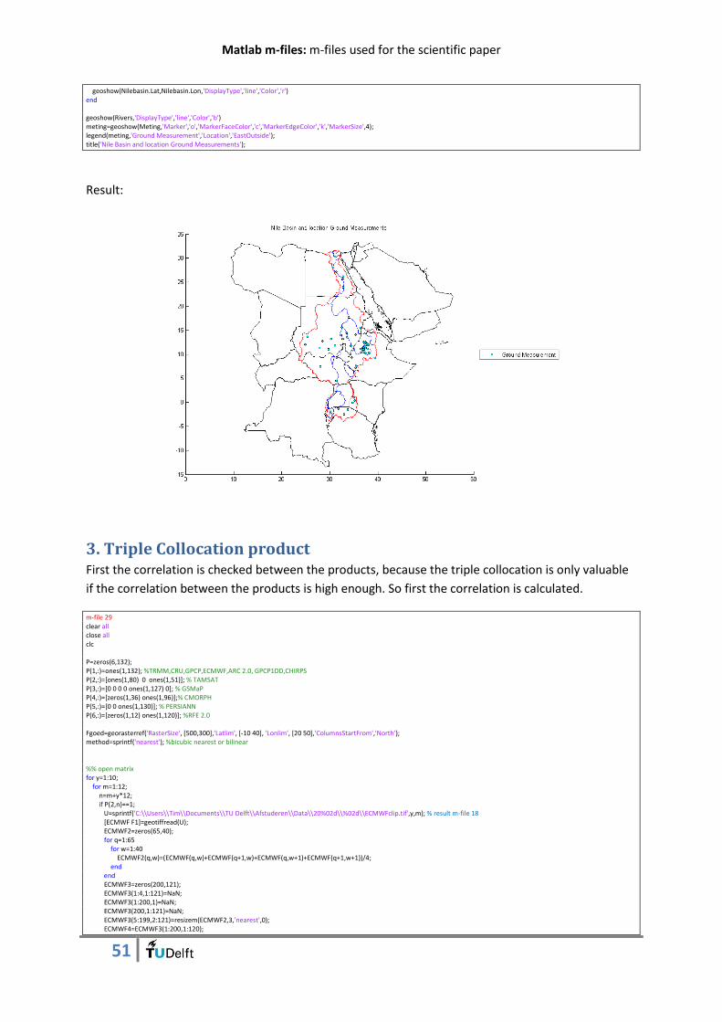
Matlab m-files: m-files used for the scientific paper

51

geoshow(Nilebasin.Lat,Nilebasin.Lon,'DisplayType','line','Color','r') end geoshow(Rivers,'DisplayType','line','Color','b') meting=geoshow(Meting,'Marker','o','MarkerFaceColor','c','MarkerEdgeColor','k','MarkerSize',4); legend(meting,'Ground Measurement','Location','EastOutside'); title('Nile Basin and location Ground Measurements');

Result:

3. Triple Collocation product First the correlation is checked between the products, because the triple collocation is only valuable

if the correlation between the products is high enough. So first the correlation is calculated.

m-file 29 clear all close all clc P=zeros(6,132); P(1,:)=ones(1,132); %TRMM,CRU,GPCP,ECMWF,ARC 2.0, GPCP1DD,CHIRPS P(2,:)=[ones(1,80) 0 ones(1,51)]; % TAMSAT P(3,:)=[0 0 0 0 ones(1,127) 0]; % GSMaP P(4,:)=[zeros(1,36) ones(1,96)];% CMORPH P(5,:)=[0 0 ones(1,130)]; % PERSIANN P(6,:)=[zeros(1,12) ones(1,120)]; %RFE 2.0 Fgoed=georasterref('RasterSize', [500,300],'Latlim', [-10 40], 'Lonlim', [20 50],'ColumnsStartFrom','North'); method=sprintf('nearest'); %bicubic nearest or bilinear %% open matrix for y=1:10; for m=1:12; n=m+y*12; if P(2,n)==1; U=sprintf('C:\\Users\\Tim\\Documents\\TU Delft\\Afstuderen\\Data\\20%02d\\%02d\\ECMWFclip.tif',y,m); % result m-file 18 [ECMWF F1]=geotiffread(U); ECMWF2=zeros(65,40); for q=1:65 for w=1:40 ECMWF2(q,w)=(ECMWF(q,w)+ECMWF(q+1,w)+ECMWF(q,w+1)+ECMWF(q+1,w+1))/4; end end ECMWF3=zeros(200,121); ECMWF3(1:4,1:121)=NaN; ECMWF3(1:200,1)=NaN; ECMWF3(200,1:121)=NaN; ECMWF3(5:199,2:121)=resizem(ECMWF2,3,'nearest',0); ECMWF4=ECMWF3(1:200,1:120);

Matlab m-files: m-files used for the scientific paper

52

ECMWF=resizem(ECMWF4,1/3,method,0); ECMWFcor(:,:,n)=ECMWF; U=sprintf('C:\\Users\\Tim\\Documents\\TU Delft\\Afstuderen\\Data\\20%02d\\%02d\\CRUclip.tif',y,m); % result m-file 18 [CRU F4]=geotiffread(U); CRU=resizem(CRU,2/3,'nearest',0); CRUcor(:,:,n)=CRU; U=sprintf('20%02d\\%02d\\CHIRPSclip.tif',j,m); % result m-file 18 [CHIRPS F7]=geotiffread(U); CHIRPSgoed(:,:,n)=resizem(CHIRPS,(0.2)/3,'nearest',0); CHIRPScor(:,:,n)=CHIRPSgoed(:,:,n); %for TRMM instead of CHIRPS %U=sprintf('20%02d\\%02d\\TRMMclip.tif',j,m); % result m-file 18 % [TRMM F7]=geotiffread(U); %TRMMgoed(:,:,n)=resizem(TRMM,1/3,'nearest',0); %CHIRPScor(:,:,n)=TRMMgoed(:,:,n); %for TAMSAT instead of CHIRPS %t=y*12+m; %k=y*12+m; %U=sprintf('20%02d\\%02d\\TAMSATclip.tif',y,m); % result m-file 18 %[TAMSAT F12]=geotiffread(U); %TAMSAT=resizem(TAMSAT,3,'nearest',0); %TAMSAT2=zeros(4000,2400); %TAMSAT2(1:430,1:2400)=NaN; %TAMSAT2(156:end,:)=TAMSAT(1:end-16,17:end-11); %grid=0.75; %B=zeros(66,40); %aantal=grid/0.0125; %A=size(B); %for i=1:A(1); % for o=1:A(2); % aveTAMSAT(i,o)=nanmean(nanmean(TAMSAT2((i-1)*aantal+1:i*aantal,(o-1)*aantal+1:o*aantal))); % end %end %TAMSATgoed(:,:,n)=aveTAMSAT; %CHIRPScor(:,:,n)=TAMSATgoed(:,:,n); end end end for r=1:66; h=waitbar(0,'Please Wait....'); steps=500; waitbar(r/steps) for k=1:40; for i=1:n; ECMWFvec(i)=ECMWFcor(r,k,i); CHIRPSvec(i)=CHIRPScor(r,k,i); CRUvec(i)=CRUcor(r,k,i); end ECMWFvec=ECMWFvec'; CRUvec=CRUvec'; CHIRPSvec=CHIRPSvec'; M=corrcoef([ECMWFvec CHIRPSvec]); N=corrcoef([CHIRPSvec CRUvec]); B=corrcoef([CRUvec ECMWFvec]); ECMWFCHIRPS(r,k)=M(2,1); CHIRPSCRU(r,k)=N(2,1); CRUECMWF(r,k)=B(2,1); ECMWFvec=0; CHIRPSvec=0; CRUvec=0; end close(h) end save('ECMWFCHIRPS075.mat','ECMWFCHIRPS'); save('CHIRPSCRU075.mat','CHIRPSCRU'); save('CRUECMWF075.mat','CRUECMWF'); %% figure Nilebasin=shaperead('Nilebasin','UseGeoCoords',true); inLat=Nilebasin.Lat; inLon=Nilebasin.Lon; gridDensity=1.33333333333333; [inGrid,InRefVec]=vec2mtx(inLat,inLon,gridDensity); Masker=zeros(66,40); Mask=imfill(inGrid,'holes'); a1=floor(Nilebasin.BoundingBox(1,2)*10)/1.333333333333333-0.2; a2=floor(Nilebasin.BoundingBox(2,2)*10)/1.333333333333333+0.2; h=subplot_tight(1,3,1,.05) geoshow(ECMWFCHIRPS,F1,'DisplayType','Texturemap') geoshow(Nilebasin.Lat,Nilebasin.Lon,'DisplayType','line','Color','k','LineWidth',3); axis([22 45 -8 35]); caxis([0 1]); title('ECMWF and CHIRPS','FontSize',12,'FontWeight','Bold'); h=subplot_tight(1,3,2,.05) geoshow(CRUECMWF,F1,'DisplayType','Texturemap') geoshow(Nilebasin.Lat,Nilebasin.Lon,'DisplayType','line','Color','k','LineWidth',3); axis([22 45 -8 35]); caxis([0 1]); title('CRU and ECMWF','FontSize',12,'FontWeight','Bold'); h=subplot_tight(1,3,3,.05)

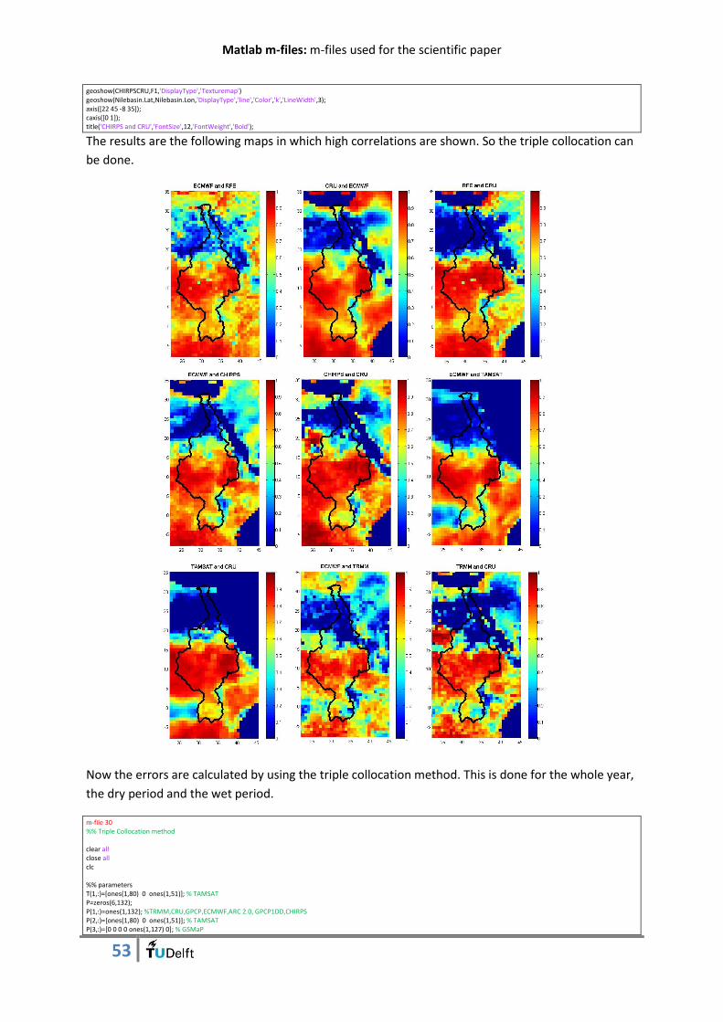
Matlab m-files: m-files used for the scientific paper

53

geoshow(CHIRPSCRU,F1,'DisplayType','Texturemap') geoshow(Nilebasin.Lat,Nilebasin.Lon,'DisplayType','line','Color','k','LineWidth',3); axis([22 45 -8 35]); caxis([0 1]); title('CHIRPS and CRU','FontSize',12,'FontWeight','Bold');

The results are the following maps in which high correlations are shown. So the triple collocation can

be done.

Now the errors are calculated by using the triple collocation method. This is done for the whole year,

the dry period and the wet period.

m-file 30 %% Triple Collocation method clear all close all clc %% parameters T(1,:)=[ones(1,80) 0 ones(1,51)]; % TAMSAT P=zeros(6,132); P(1,:)=ones(1,132); %TRMM,CRU,GPCP,ECMWF,ARC 2.0, GPCP1DD,CHIRPS P(2,:)=[ones(1,80) 0 ones(1,51)]; % TAMSAT P(3,:)=[0 0 0 0 ones(1,127) 0]; % GSMaP

Matlab m-files: m-files used for the scientific paper

54

P(4,:)=[zeros(1,36) ones(1,96)];% CMORPH P(5,:)=[0 0 ones(1,130)]; % PERSIANN P(6,:)=[zeros(1,12) ones(1,120)]; %RFE 2.0 Fgoed=georasterref('RasterSize', [66,40],'Latlim', [-10 40], 'Lonlim', [20 50],'ColumnsStartFrom','North'); method=sprintf('nearest'); %bicubic nearest or bilinear X=[]; Y=[]; F=zeros(66,40); Z=[]; D=zeros(66,40); h=waitbar(0,'please wait...' ); for j=0:10; for m=1:12; n=m+j*12; waitbar(n/132,h); if T(1,n)==1; U=sprintf('20%02d\\%02d\\CRUclip.tif',j,m); % result m-file 18 [CRU F4]=geotiffread(U); CRUgoed(:,:,n)=resizem(CRU,2/3,method,0); U=sprintf('20%02d\\%02d\\ECMWFclip.tif',j,m); % result m-file 18 [ECMWF F1]=geotiffread(U); ECMWF2=zeros(65,40); for q=1:65 for w=1:40 ECMWF2(q,w)=(ECMWF(q,w)+ECMWF(q+1,w)+ECMWF(q,w+1)+ECMWF(q+1,w+1))/4; end end ECMWF3=zeros(200,121); ECMWF3(1:4,1:121)=NaN; ECMWF3(1:200,1)=NaN; ECMWF3(200,1:121)=NaN; ECMWF3(5:199,2:121)=resizem(ECMWF2,3,method,0); ECMWF4=ECMWF3(1:200,1:120); ECMWFgoed(:,:,n)=resizem(ECMWF4,1/3,method,0); U=sprintf('20%02d\\%02d\\CHIRPSclip.tif',j,m); % result m-file 18 [CHIRPS F7]=geotiffread(U); CHIRPSgoed(:,:,n)=resizem(CHIRPS,(0.2)/3,method,0); %For TRMM instead of CHIRPS %U=sprintf('20%02d\\%02d\\TRMMclip.tif',j,m); % result m-file 18 % [TRMM F7]=geotiffread(U); %TRMMgoed(:,:,n)=resizem(TRMM,1/3,method,0); %For TAMSAT instead of CHIRPS % t=j*12+m; % k=j*12+m; %U=sprintf('20%02d\\%02d\\TAMSATclip.tif',j,m); % result m-file 18 %[TAMSAT F12]=geotiffread(U); %TAMSAT=resizem(TAMSAT,3,method,0); %TAMSAT2=zeros(4000,2400); %TAMSAT2(1:430,1:2400)=NaN; %TAMSAT2(156:end,:)=TAMSAT(1:end-16,17:end-11); %grid=0.75; %B=zeros(66,40); %aantal=grid/0.0125; %A=size(B); %for i=1:A(1); % for o=1:A(2); % aveTAMSAT(i,o)=nanmean(nanmean(TAMSAT2((i-1)*aantal+1:i*aantal,(o-1)*aantal+1:o*aantal))); % end %end %TAMSATgoed(:,:,n)=aveTAMSAT; end end end %% open all maps and resize Q=zeros(66,40,6); h=waitbar(0,'please wait...' ); for y=1:66; waitbar(y/66,h); for x=1:40; j=0; m=1; p=1; for j=0:10; for m=[1:4 11 12];%whole year [1:12];% wet season[5:10]% dry season [1:4 11 12]; n=m+j*12; if CHIRPSgoed(y,x,n)>0 && ECMWFgoed(y,x,n)>0 && CRUgoed(y,x,n)>0; Z(p)=CHIRPSgoed(y,x,n); Y(p)=CRUgoed(y,x,n); X(p)=ECMWFgoed(y,x,n); D(y,x)=D(y,x)+1; p=p+1; else F(y,x)=F(y,x)+1; end end end bx=1; by=1; bz=1;

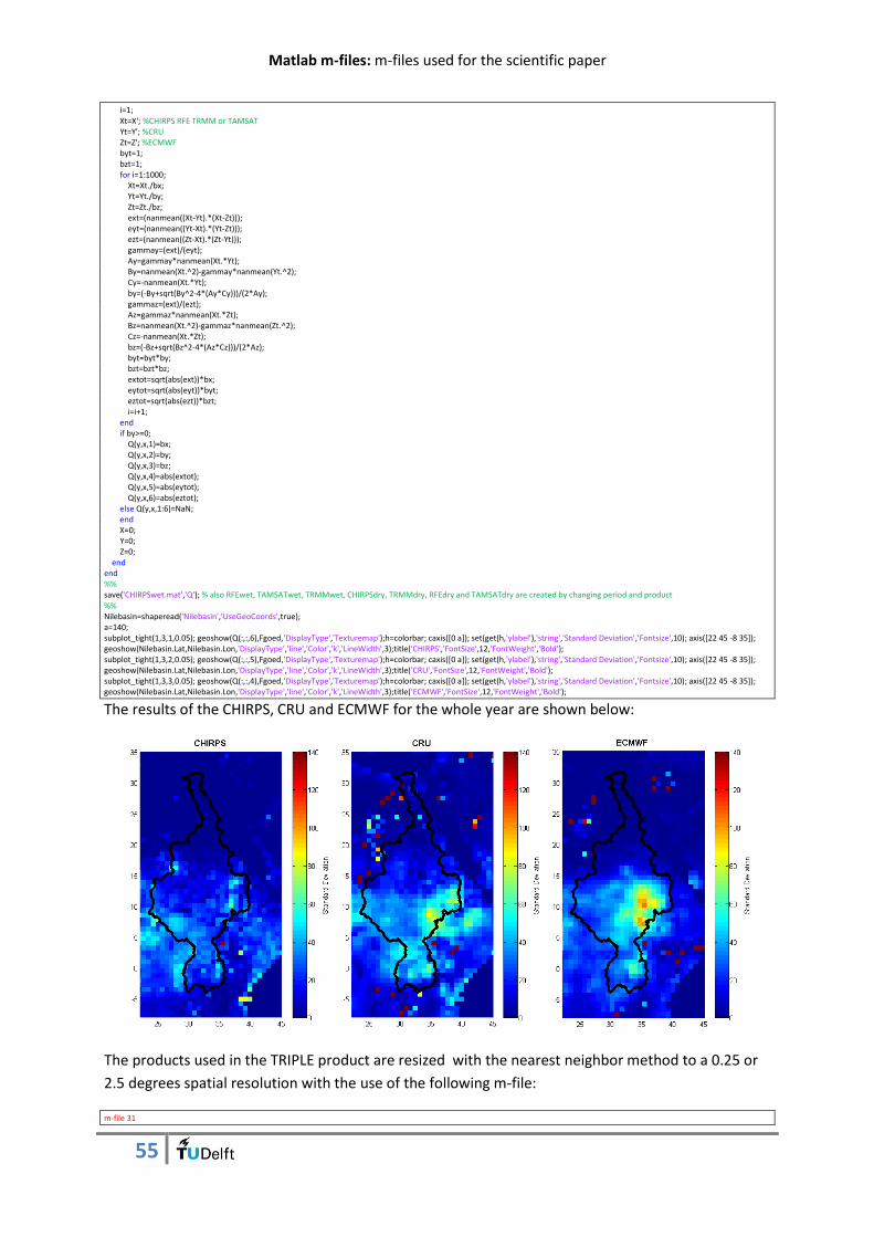
Matlab m-files: m-files used for the scientific paper

55

i=1; Xt=X'; %CHIRPS RFE TRMM or TAMSAT Yt=Y'; %CRU Zt=Z'; %ECMWF byt=1; bzt=1; for i=1:1000; Xt=Xt./bx; Yt=Yt./by; Zt=Zt./bz; ext=(nanmean((Xt-Yt).*(Xt-Zt))); eyt=(nanmean((Yt-Xt).*(Yt-Zt))); ezt=(nanmean((Zt-Xt).*(Zt-Yt))); gammay=(ext)/(eyt); Ay=gammay*nanmean(Xt.*Yt); By=nanmean(Xt.^2)-gammay*nanmean(Yt.^2); Cy=-nanmean(Xt.*Yt); by=(-By+sqrt(By^2-4*(Ay*Cy)))/(2*Ay); gammaz=(ext)/(ezt); Az=gammaz*nanmean(Xt.*Zt); Bz=nanmean(Xt.^2)-gammaz*nanmean(Zt.^2); Cz=-nanmean(Xt.*Zt); bz=(-Bz+sqrt(Bz^2-4*(Az*Cz)))/(2*Az); byt=byt*by; bzt=bzt*bz; extot=sqrt(abs(ext))*bx; eytot=sqrt(abs(eyt))*byt; eztot=sqrt(abs(ezt))*bzt; i=i+1; end if by>=0; Q(y,x,1)=bx; Q(y,x,2)=by; Q(y,x,3)=bz; Q(y,x,4)=abs(extot); Q(y,x,5)=abs(eytot); Q(y,x,6)=abs(eztot); else Q(y,x,1:6)=NaN; end X=0; Y=0; Z=0; end end %% save('CHIRPSwet.mat','Q'); % also RFEwet, TAMSATwet, TRMMwet, CHIRPSdry, TRMMdry, RFEdry and TAMSATdry are created by changing period and product %% Nilebasin=shaperead('Nilebasin','UseGeoCoords',true); a=140; subplot_tight(1,3,1,0.05); geoshow(Q(:,:,6),Fgoed,'DisplayType','Texturemap');h=colorbar; caxis([0 a]); set(get(h,'ylabel'),'string','Standard Deviation','Fontsize',10); axis([22 45 -8 35]); geoshow(Nilebasin.Lat,Nilebasin.Lon,'DisplayType','line','Color','k','LineWidth',3);title('CHIRPS','FontSize',12,'FontWeight','Bold'); subplot_tight(1,3,2,0.05); geoshow(Q(:,:,5),Fgoed,'DisplayType','Texturemap');h=colorbar; caxis([0 a]); set(get(h,'ylabel'),'string','Standard Deviation','Fontsize',10); axis([22 45 -8 35]); geoshow(Nilebasin.Lat,Nilebasin.Lon,'DisplayType','line','Color','k','LineWidth',3);title('CRU','FontSize',12,'FontWeight','Bold'); subplot_tight(1,3,3,0.05); geoshow(Q(:,:,4),Fgoed,'DisplayType','Texturemap');h=colorbar; caxis([0 a]); set(get(h,'ylabel'),'string','Standard Deviation','Fontsize',10); axis([22 45 -8 35]); geoshow(Nilebasin.Lat,Nilebasin.Lon,'DisplayType','line','Color','k','LineWidth',3);title('ECMWF','FontSize',12,'FontWeight','Bold');

The results of the CHIRPS, CRU and ECMWF for the whole year are shown below:

The products used in the TRIPLE product are resized with the nearest neighbor method to a 0.25 or

2.5 degrees spatial resolution with the use of the following m-file:

m-file 31

Matlab m-files: m-files used for the scientific paper

56

clear all; close all; clc; grid=0.25; B=zeros(50/grid,30/grid); maat=025; T(1,:)=[ones(1,80) 0 ones(1,51)]; % TAMSAT T(2,:)=[0 0 0 0 ones(1,127) 0]; % GSMaP T(3,:)=[zeros(1,36) ones(1,96)];% CMORPH T(4,:)=[0 0 ones(1,130)]; % PERSIANN T(5,:)=[zeros(1,12) ones(1,120)]; %RFE 2.0 %% TRMM for y=0:10 for m=1:12 U=sprintf('C:\\Users\\Tim\\Documents\\TU Delft\\Afstuderen\\Data\\20%02d\\%02d\\TRMMclip.tif',y,m); % result m-file 18 [TRMM F1]=geotiffread(U); aveTRMM=TRMM; A=size(B); k=y*12+m; opslaan=sprintf('GridBlock\\Triplekaarten\\TRMM%03d.mat',k); save(opslaan,'aveTRMM'); end end %% GPCP for y=0:10 for m=1:12 U=sprintf('C:\\Users\\Tim\\Documents\\TU Delft\\Afstuderen\\Data\\20%02d\\%02d\\GPCPclip.tif',y,m); % result m-file 18 [GPCP F2]=geotiffread(U); aveGPCP=resizem(GPCP,10,'nearest',0); k=y*12+m; opslaan=sprintf('GridBlock\\Triplekaarten\\GPCP%03d.mat',k); save(opslaan,'aveGPCP'); end end %% GPCP1DD for y=0:10 for m=1:12 U=sprintf('C:\\Users\\Tim\\Documents\\TU Delft\\Afstuderen\\Data\\20%02d\\%02d\\GPCP1DDclip.tif',y,m); % result m-file 18 [GPCP1DD F3]=geotiffread(U); GPCP1DD2=resizem(GPCP1DD,4,'nearest',0); aveGPCP1DD=GPCP1DD2; k=y*12+m; opslaan=sprintf('GridBlock\\Triplekaarten\\GPCP1DD%03d.mat',k); save(opslaan,'aveGPCP1DD'); end end %% CRU for y=0:10 for m=1:12 U=sprintf('C:\\Users\\Tim\\Documents\\TU Delft\\Afstuderen\\Data\\20%02d\\%02d\\CRUclip.tif',y,m); % result m-file 18 [CRU F4]=geotiffread(U); aveCRU=resizem(CRU,2,'nearest',0); k=y*12+m; opslaan=sprintf('GridBlock\\Triplekaarten\\CRU%03d.mat',k); save(opslaan,'aveCRU'); end end %% ECMWF for y=0:10 for m=1:12 U=sprintf('C:\\Users\\Tim\\Documents\\TU Delft\\Afstuderen\\Data\\20%02d\\%02d\\ECMWFclip.tif',y,m); % result m-file 18 [ECMWF F5]=geotiffread(U); ECMWF2=zeros(65,40); for q=1:65 for w=1:40 ECMWF2(q,w)=(ECMWF(q,w)+ECMWF(q+1,w)+ECMWF(q,w+1)+ECMWF(q+1,w+1))/4; end end ECMWF3=zeros(200,121); ECMWF3(1:4,1:121)=NaN; ECMWF3(1:200,1)=NaN; ECMWF3(200,1:121)=NaN; ECMWF3(5:199,2:121)=resizem(ECMWF2,3,'nearest',0); ECMWF4=ECMWF3(1:200,1:120); aveECMWF=ECMWF4; k=y*12+m; opslaan=sprintf('GridBlock\\Triplekaarten\\ECMWF%03d.mat',k); save(opslaan,'aveECMWF'); end end %% ARC 2.0 for y=0:10 for m=1:12 U=sprintf('C:\\Users\\Tim\\Documents\\TU Delft\\Afstuderen\\Data\\20%02d\\%02d\\ARCclip.tif',y,m); % result m-file 18 [ARC F6]=geotiffread(U); ARC2=zeros(500,300); for q=1:500 for w=1:300 ARC2(q,w)=(ARC(q,w)+ARC(q+1,w)+ARC(q,w+1)+ARC(q+1,w+1))/4;

Matlab m-files: m-files used for the scientific paper

57

end end ARC2=resizem(ARC2,2,'nearest',0); aantal=grid/0.05; A=size(B); for i=1:A(1); for j=1:A(2); aveARC(i,j)=nanmean(nanmean(ARC2((i-1)*aantal+1:i*aantal,(j-1)*aantal+1:j*aantal))); end end k=y*12+m; opslaan=sprintf('GridBlock\\Triplekaarten\\ARC%03d.mat',k); save(opslaan,'aveARC'); end end %% CHIRPS for y=0:10 for m=1:12 U=sprintf('C:\\Users\\Tim\\Documents\\TU Delft\\Afstuderen\\Data\\20%02d\\%02d\\CHIRPSclip.tif',y,m); % result m-file 18 [CHIRPS F7]=geotiffread(U); aantal=grid/0.05; A=size(B); for i=1:A(1); for j=1:A(2); aveCHIRPS(i,j)=nanmean(nanmean(CHIRPS((i-1)*aantal+1:i*aantal,(j-1)*aantal+1:j*aantal))); end end k=y*12+m; opslaan=sprintf('GridBlock\\Triplekaarten\\CHIRPS%03d.mat',k); save(opslaan,'aveCHIRPS'); end end %% RFE for y=0:10 for m=1:12 t=y*12+m; k=y*12+m; if T(5,t)==1; U=sprintf('C:\\Users\\Tim\\Documents\\TU Delft\\Afstuderen\\Data\\20%02d\\%02d\\FEWSNETclip.tif',y,m); % result m-file 18 [RFE F8]=geotiffread(U); RFE2=zeros(500,300); for q=1:500 for w=1:300 RFE2(q,w)=(RFE(q,w)+RFE(q+1,w)+RFE(q,w+1)+RFE(q+1,w+1))/4; end end RFE2=resizem(RFE2,2,'nearest',0); aantal=grid/0.05; A=size(B); for i=1:A(1); for j=1:A(2); aveRFE(i,j)=nanmean(nanmean(RFE2((i-1)*aantal+1:i*aantal,(j-1)*aantal+1:j*aantal))); end end k=y*12+m; opslaan=sprintf('GridBlock\\Triplekaarten\\RFE%03d.mat',k); save(opslaan,'aveRFE'); end end end %% PERSIANN for y=0:10 for m=1:12 t=y*12+m; k=y*12+m; if T(4,t)==1; U=sprintf('C:\\Users\\Tim\\Documents\\TU Delft\\Afstuderen\\Data\\20%02d\\%02d\\PERSIANNclip.tif',y,m); % result m-file 18 [PERSIANN F9]=geotiffread(U); avePERSIANN=PERSIANN; k=y*12+m; opslaan=sprintf('GridBlock\\Triplekaarten\\PERSIANN%03d.mat',k); save(opslaan,'avePERSIANN'); end end end %% CMORPH for y=0:10 for m=1:12 t=y*12+m; k=y*12+m; if T(3,t)==1; U=sprintf('C:\\Users\\Tim\\Documents\\TU Delft\\Afstuderen\\Data\\20%02d\\%02d\\CMORPHclip.tif',y,m); % result m-file 18 [CMORPH F10]=geotiffread(U); CMORPH2=zeros(200,120); CMORPH2(1:4,:)=NaN; CMORPH2(5:200,:)=CMORPH; aveCMORPH=CMORPH2; k=y*12+m; opslaan=sprintf('GridBlock\\Triplekaarten\\CMORPH%03d.mat',k); save(opslaan,'aveCMORPH');

Matlab m-files: m-files used for the scientific paper

58

end end end %% GSMaP for y=0:10 for m=1:12 t=y*12+m; k=y*12+m; if T(2,t)==1; U=sprintf('C:\\Users\\Tim\\Documents\\TU Delft\\Afstuderen\\Data\\20%02d\\%02d\\GSMaPclip.tif',y,m); % result m-file 18 [GSMaP F11]=geotiffread(U); GSMaP=resizem(GSMaP,2,'nearest',0); aantal=grid/0.05; A=size(B); for i=1:A(1); for j=1:A(2); aveGSMaP(i,j)=nanmean(nanmean(GSMaP((i-1)*aantal+1:i*aantal,(j-1)*aantal+1:j*aantal))); end end k=y*12+m; opslaan=sprintf('GridBlock\\Triplekaarten\\GSMaP%03d.mat',k); save(opslaan,'aveGSMaP'); end end end clearvars ECMWF ECMWF2 ECMWF3 ECMWF4 GPCP1DD GPCP1DD2 PERSIANN ARC ARC2 CHIRPS CRU F1 F2 F3 F4 F5 GSMaP TRMM %% TAMSAT for y=0:10 for m=1:12 t=y*12+m; k=y*12+m; if T(1,t)==1; U=sprintf('C:\\Users\\Tim\\Documents\\TU Delft\\Afstuderen\\Data\\20%02d\\%02d\\TAMSATclip.tif',y,m); % result m-file 18 [TAMSAT F12]=geotiffread(U); TAMSAT=resizem(TAMSAT,3,'nearest',0); TAMSAT2=zeros(4000,2400); TAMSAT2(1:430,1:2400)=NaN; TAMSAT2(156:end,:)=TAMSAT(1:end-16,17:end-11); aantal=grid/0.0125; A=size(B); for i=1:A(1); for j=1:A(2); aveTAMSAT(i,j)=nanmean(nanmean(TAMSAT2((i-1)*aantal+1:i*aantal,(j-1)*aantal+1:j*aantal))); end end k=y*12+m; opslaan=sprintf('GridBlock\\Triplekaarten\\TAMSAT%03d.mat',k); save(opslaan,'aveTAMSAT'); end end end %% GPCC for y=0:10 for m=1:12 U=sprintf('C:\\Users\\Tim\\Documents\\TU Delft\\Afstuderen\\Data\\20%02d\\%02d\\GPCCclip.tif',y,m); % result m-file 17 [GPCC F2]=geotiffread(U); aveGPCC=resizem(GPCC,2,'nearest',0); k=y*12+m; opslaan=sprintf('GridBlock\\Triplekaarten\\GPCC%03d.mat',k); save(opslaan,'aveGPCC'); end end

By using these errors maps (CHIRPSdry.mat, TAMSATdry.mat, TRMMdry.mat, RFEdry.mat,

CHIRPSwet.mat, TAMSATwet.mat, TRMMwet.mat, and RFEwet.mat), the triple collocation products

was made with the following m-file:

m-file 32 clear all; close all; clc; %calculating the averages over the period, is needed for the relative errors for k=1:132; open=sprintf('C:\\Users\\Tim\\Documents\\TU Delft\\Afstuderen\\Data\\GridBlock\\Triplekaarten\\TRMM%03d',k); % result m-file 31 load(open); TRMM=resizem(aveTRMM,1/3,'nearest'); TRMMtot(:,:,k)=TRMM; end for m=5:10; k=[0+m 12+m 24+m 36+m 48+m 60+m 72+m 84+m 96+m 108+m 120+m]; TRMMwet(:,:)=nanmean(TRMMtot(:,:,k),3); end for m=[1:4 11 12]; o=[0+m 12+m 24+m 36+m 48+m 60+m 72+m 84+m 96+m 108+m 120+m];

Matlab m-files: m-files used for the scientific paper

59

TRMMdry(:,:)=nanmean(TRMMtot(:,:,o),3); end for k=1:132; open=sprintf('C:\\Users\\Tim\\Documents\\TU Delft\\Afstuderen\\Data\\GridBlock\\Triplekaarten\\CRU%03d',k); % result m-file 31 load(open); CRU=resizem(aveCRU,1/3,'nearest'); CRUtot(:,:,k)=CRU; end for m=5:10; k=[0+m 12+m 24+m 36+m 48+m 60+m 72+m 84+m 96+m 108+m 120+m]; CRUwet(:,:)=nanmean(CRUtot(:,:,k),3); end for m=[1:4 11 12]; o=[0+m 12+m 24+m 36+m 48+m 60+m 72+m 84+m 96+m 108+m 120+m]; CRUdry(:,:)=nanmean(CRUtot(:,:,o),3); end for k=1:132; open=sprintf('C:\\Users\\Tim\\Documents\\TU Delft\\Afstuderen\\Data\\GridBlock\\Triplekaarten\\ECMWF%03d',k); % result m-file 31 load(open); ECMWF=resizem(aveECMWF,1/3,'nearest'); ECMWFtot(:,:,k)=ECMWF; end for m=5:10; k=[0+m 12+m 24+m 36+m 48+m 60+m 72+m 84+m 96+m 108+m 120+m]; ECMWFwet(:,:)=nanmean(ECMWFtot(:,:,k),3); end for m=[1:4 11 12]; o=[0+m 12+m 24+m 36+m 48+m 60+m 72+m 84+m 96+m 108+m 120+m]; ECMWFdry(:,:)=nanmean(ECMWFtot(:,:,o),3); end for k=1:132; open=sprintf('C:\\Users\\Tim\\Documents\\TU Delft\\Afstuderen\\Data\\GridBlock\\Triplekaarten\\CHIRPS%03d',k); % result m-file 31 load(open); CHIRPS=resizem(aveCHIRPS,1/3,'nearest'); CHIRPStot(:,:,k)=CHIRPS; end for m=5:10; k=[0+m 12+m 24+m 36+m 48+m 60+m 72+m 84+m 96+m 108+m 120+m]; CHIRPSwet(:,:)=nanmean(CHIRPStot(:,:,k),3); end for m=[1:4 11 12]; o=[0+m 12+m 24+m 36+m 48+m 60+m 72+m 84+m 96+m 108+m 120+m]; CHIRPSdry(:,:)=nanmean(CHIRPStot(:,:,o),3); end RFEtot=zeros(66,40,132); for k=13:132; open=sprintf('C:\\Users\\Tim\\Documents\\TU Delft\\Afstuderen\\Data\\GridBlock\\Triplekaarten\\RFE%03d',k); % result m-file 31 load(open); RFE=resizem(aveRFE,1/3,'nearest'); RFEtot(:,:,1:12)=NaN; RFEtot(:,:,k)=RFE; end for m=5:10; k=[0+m 12+m 24+m 36+m 48+m 60+m 72+m 84+m 96+m 108+m 120+m]; RFEwet(:,:)=nanmean(RFEtot(:,:,k),3); end for m=[1:4 11 12]; o=[0+m 12+m 24+m 36+m 48+m 60+m 72+m 84+m 96+m 108+m 120+m]; RFEdry(:,:)=nanmean(RFEtot(:,:,o),3); end for k=[1:80 82:132]; open=sprintf('C:\\Users\\Tim\\Documents\\TU Delft\\Afstuderen\\Data\\GridBlock\\Triplekaarten\\TAMSAT%03d',k); % result m-file 31 load(open); TAMSAT=resizem(aveTAMSAT,1/3,'nearest'); TAMSATtot(:,:,k)=TAMSAT; end TAMSATtot(:,:,81)=NaN; for m=5:10; k=[0+m 12+m 24+m 36+m 48+m 60+m 72+m 84+m 96+m 108+m 120+m]; TAMSATwet(:,:)=nanmean(TAMSATtot(:,:,k),3); end for m=[1:4 11 12]; o=[0+m 12+m 24+m 36+m 48+m 60+m 72+m 84+m 96+m 108+m 120+m]; TAMSATdry(:,:)=nanmean(TAMSATtot(:,:,o),3); end %% load estimated errors maps load('ProductTriple/RFEwet','Q'); % result m-file 30 Qrfewet(:,:)=Q(:,:,4); Q=0; load('ProductTriple/CHIRPSwet','Q'); % result m-file 30 Qchirpswet(:,:)=Q(:,:,4); Q=0; load('ProductTriple/CHIRPSwet','Q'); % result m-file 30 Qcruwet(:,:)=Q(:,:,5); Q=0; load('ProductTriple/CHIRPSwet','Q'); % result m-file 30 Qecmwfwet(:,:)=Q(:,:,6); Q=0; load('ProductTriple/TAMSATwet','Q'); % result m-file 30 Qtamsatwet(:,:)=Q(:,:,4); Q=0; load('ProductTriple/TRMMwet','Q'); % result m-file 30 Qtrmmwet(:,:)=Q(:,:,4); Q=0;

Matlab m-files: m-files used for the scientific paper

60

load('ProductTriple/RFEdry','Q'); % result m-file 30 Qrfedry(:,:)=Q(:,:,4); Q=0; load('ProductTriple/CHIRPSdry','Q'); % result m-file 30 Qchirpsdry(:,:)=Q(:,:,4); Q=0; load('ProductTriple/CHIRPSdry','Q'); % result m-file 30 Qcrudry(:,:)=Q(:,:,5); Q=0; load('ProductTriple/CHIRPSdry','Q'); % result m-file 30 Qecmwfdry(:,:)=Q(:,:,6); Q=0; load('ProductTriple/TAMSATdry','Q'); % result m-file 30 Qtamsatdry(:,:)=Q(:,:,4); Q=0; load('ProductTriple/TRMMdry','Q'); % result m-file 30 Qtrmmdry(:,:)=Q(:,:,4); Q=0; %calculating relative errors P(:,:,1)=Qrfewet(:,:)./RFEwet(:,:); P(:,:,2)=Qchirpswet(:,:)./CHIRPSwet(:,:); P(:,:,3)=Qcruwet(:,:)./CRUwet(:,:); P(:,:,4)=Qecmwfwet(:,:)./ECMWFwet(:,:); P(:,:,5)=Qtamsatwet(:,:)./TAMSATwet(:,:); P(:,:,6)=Qtrmmwet(:,:)./TRMMwet(:,:); P(:,:,7)=Qrfedry(:,:)./RFEdry(:,:); P(:,:,8)=Qchirpsdry(:,:)./CHIRPSdry(:,:); P(:,:,9)=Qcrudry(:,:)./CRUdry(:,:); P(:,:,10)=Qecmwfdry(:,:)./ECMWFdry(:,:); P(:,:,11)=Qtamsatdry(:,:)./TAMSATdry(:,:); P(:,:,12)=Qtrmmdry(:,:)./TRMMdry(:,:); % assign pixels with the product with the lowest relative error for x=1:66; for y=1:40; minimaalwet(x,y)=nanmin(P(x,y,1:6)); end end for x=1:66; for y=1:40; minimaaldry(x,y)=nanmin(P(x,y,7:12)); end end for x=1:66; for y=1:40; if minimaalwet(x,y)==P(x,y,1); welkewet(x,y)=1; elseif minimaalwet(x,y)==P(x,y,2); welkewet(x,y)=2; elseif minimaalwet(x,y)==P(x,y,3); welkewet(x,y)=3; elseif minimaalwet(x,y)==P(x,y,4); welkewet(x,y)=4; elseif minimaalwet(x,y)==P(x,y,5); welkewet(x,y)=5; elseif minimaalwet(x,y)==P(x,y,6); welkewet(x,y)=6; end end end for x=1:66; for y=1:40; if minimaaldry(x,y)==P(x,y,7); welkedry(x,y)=1; elseif minimaaldry(x,y)==P(x,y,8); welkedry(x,y)=2; elseif minimaaldry(x,y)==P(x,y,9); welkedry(x,y)=3; elseif minimaaldry(x,y)==P(x,y,10); welkedry(x,y)=4; elseif minimaaldry(x,y)==P(x,y,11); welkedry(x,y)=5; elseif minimaaldry(x,y)==P(x,y,12); welkedry(x,y)=6; end end end %% plot map with the assigned product subplot(1,2,1); R2 = georasterref('RasterSize', size(welkewet),'Latlim', [-9.5 40], 'Lonlim', [20 50],'ColumnsStartFrom','north'); h=geoshow(welkewet,R2,'DisplayType','Texturemap'); Nilebasin = shaperead('Layers\Sub\Nilebasin','UseGeoCoords',true); geoshow(Nilebasin.Lat,Nilebasin.Lon,'DisplayType','line','Color','b') subplot(1,2,2); h=geoshow(welkedry,R2,'DisplayType','Texturemap'); Nilebasin = shaperead('Layers\Sub\Nilebasin','UseGeoCoords',true); geoshow(Nilebasin.Lat,Nilebasin.Lon,'DisplayType','line','Color','b') geotiffwrite('nattriple.tif',welkewet,R2); %% Make TRIPLE product

Matlab m-files: m-files used for the scientific paper

61

TRIPLE2=resizem(welkewet,3,'nearest'); TRIPLE3(1:198,:)=TRIPLE2; TRIPLE3(199:200,:)=NaN; welkewet=TRIPLE3; TRIPLE2=resizem(welkedry,3,'nearest'); TRIPLE3(1:198,:)=TRIPLE2; TRIPLE3(199:200,:)=NaN; welkedry=TRIPLE3; for j=0:10; for m=1:12; k=m+j*12; T(1,:)=[zeros(1,12) ones(1,120)]; %RFE 2.0 T(2,:)=[ones(1,80) 0 ones(1,51)]; % TAMSAT U=sprintf('C:\\Users\\Tim\\Documents\\TU Delft\\Afstuderen\\Data\\GridBlock\\Kaarten025\\CHIRPS%03d.mat',k); % result m-file 33 load(U); CHIRPSgoed=aveCHIRPS; U=sprintf('C:\\Users\\Tim\\Documents\\TU Delft\\Afstuderen\\Data\\GridBlock\\Kaarten025\\CRU%03d.mat',k); % result m-file 33 load(U); CRUgoed=aveCRU; if T(1,k)==1 U=sprintf('C:\\Users\\Tim\\Documents\\TU Delft\\Afstuderen\\Data\\GridBlock\\Kaarten025\\RFE%03d.mat',k); % result m-file 33 load(U); RFEgoed=aveRFE; else RFEgoed(:,:)=CHIRPSgoed(:,:); end U=sprintf('C:\\Users\\Tim\\Documents\\TU Delft\\Afstuderen\\Data\\GridBlock\\Kaarten025\\ECMWF%03d.mat',k); % result m-file 33 load(U); ECMWFgoed=aveECMWF; U=sprintf('C:\\Users\\Tim\\Documents\\TU Delft\\Afstuderen\\Data\\GridBlock\\Kaarten025\\TRMM%03d.mat',k); % result m-file 33 load(U); TRMMgoed=aveTRMM; t=j*12+m; k=j*12+m; if T(2,k)==1 U=sprintf('C:\\Users\\Tim\\Documents\\TU Delft\\Afstuderen\\Data\\GridBlock\\Kaarten025\\TAMSAT%03d.mat',k); % result m-file 33 load(U); TAMSATgoed=aveTAMSAT; else TAMSATgoed(:,:)=CHIRPSgoed(:,:); end for x=1:200; for y=1:120; if m>=4.8 && m<=10.2; if welkewet(x,y)==1; producttriple(x,y)=RFEgoed(x,y); elseif welkewet(x,y)==2; producttriple(x,y)=CHIRPSgoed(x,y); elseif welkewet(x,y)==3; producttriple(x,y)=CRUgoed(x,y); elseif welkewet(x,y)==4; producttriple(x,y)=ECMWFgoed(x,y); elseif welkewet(x,y)==5; producttriple(x,y)=TAMSATgoed(x,y); elseif welkewet(x,y)==6; producttriple(x,y)=TRMMgoed(x,y); end else if welkedry(x,y)==1; producttriple(x,y)=RFEgoed(x,y); elseif welkedry(x,y)==2; producttriple(x,y)=CHIRPSgoed(x,y); elseif welkedry(x,y)==3; producttriple(x,y)=CRUgoed(x,y); elseif welkedry(x,y)==4; producttriple(x,y)=ECMWFgoed(x,y); elseif welkedry(x,y)==5; producttriple(x,y)=TAMSATgoed(x,y); elseif welkedry(x,y)==6; producttriple(x,y)=TRMMgoed(x,y); end end end end Eindproduct(:,:,k)=producttriple(:,:); end end Eindproduct(199:200,:,:)=NaN; save('Eindproduct.mat');

The TRIPLE endproduct is saved and also the map with the assigned products are made. This map is

shown below for the wet and dry period.

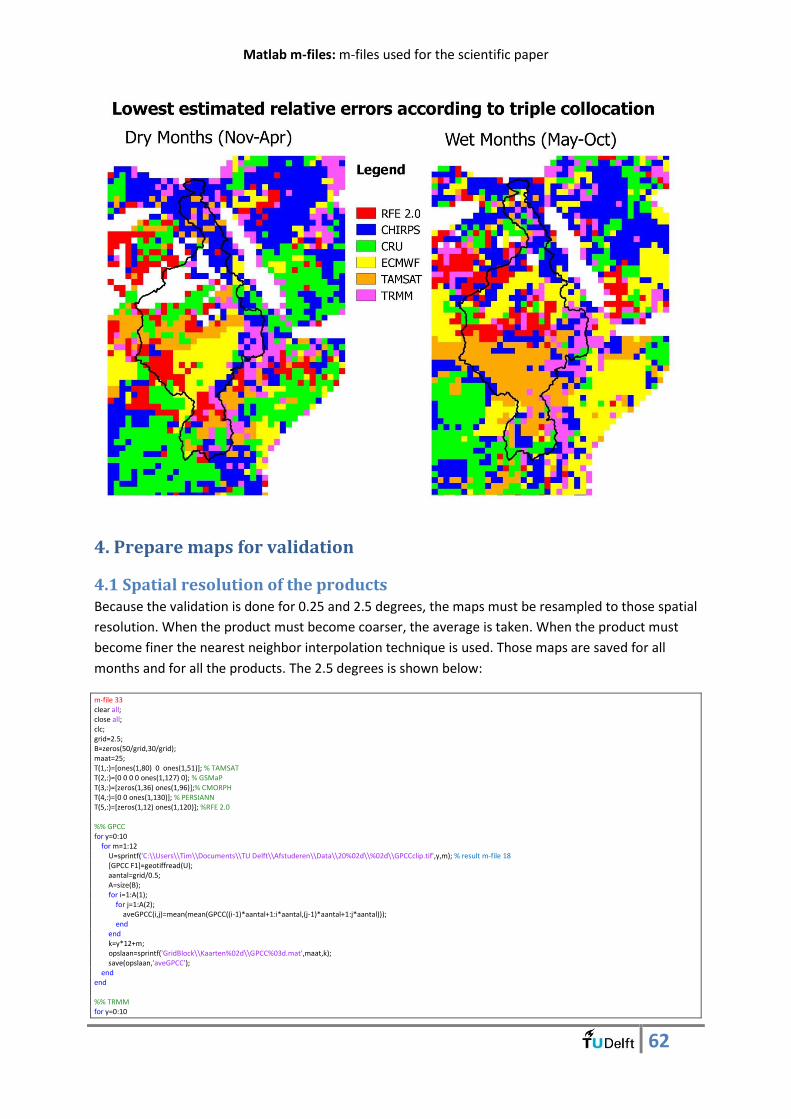
Matlab m-files: m-files used for the scientific paper

62

4. Prepare maps for validation

4.1 Spatial resolution of the products Because the validation is done for 0.25 and 2.5 degrees, the maps must be resampled to those spatial

resolution. When the product must become coarser, the average is taken. When the product must

become finer the nearest neighbor interpolation technique is used. Those maps are saved for all

months and for all the products. The 2.5 degrees is shown below:

m-file 33 clear all; close all; clc; grid=2.5; B=zeros(50/grid,30/grid); maat=25; T(1,:)=[ones(1,80) 0 ones(1,51)]; % TAMSAT T(2,:)=[0 0 0 0 ones(1,127) 0]; % GSMaP T(3,:)=[zeros(1,36) ones(1,96)];% CMORPH T(4,:)=[0 0 ones(1,130)]; % PERSIANN T(5,:)=[zeros(1,12) ones(1,120)]; %RFE 2.0 %% GPCC for y=0:10 for m=1:12 U=sprintf('C:\\Users\\Tim\\Documents\\TU Delft\\Afstuderen\\Data\\20%02d\\%02d\\GPCCclip.tif',y,m); % result m-file 18 [GPCC F1]=geotiffread(U); aantal=grid/0.5; A=size(B); for i=1:A(1); for j=1:A(2); aveGPCC(i,j)=mean(mean(GPCC((i-1)*aantal+1:i*aantal,(j-1)*aantal+1:j*aantal))); end end k=y*12+m; opslaan=sprintf('GridBlock\\Kaarten%02d\\GPCC%03d.mat',maat,k); save(opslaan,'aveGPCC'); end end %% TRMM for y=0:10

Matlab m-files: m-files used for the scientific paper

63

for m=1:12 U=sprintf('C:\\Users\\Tim\\Documents\\TU Delft\\Afstuderen\\Data\\20%02d\\%02d\\TRMMclip.tif',y,m); % result m-file 18 [TRMM F1]=geotiffread(U); aantal=grid/0.25; A=size(B); for i=1:A(1); for j=1:A(2); aveTRMM(i,j)=mean(mean(TRMM((i-1)*aantal+1:i*aantal,(j-1)*aantal+1:j*aantal))); end end k=y*12+m; opslaan=sprintf('GridBlock\\Kaarten%02d\\TRMM%03d.mat',maat,k); save(opslaan,'aveTRMM'); end end %% GPCP for y=0:10 for m=1:12 U=sprintf('C:\\Users\\Tim\\Documents\\TU Delft\\Afstuderen\\Data\\20%02d\\%02d\\GPCPclip.tif',y,m); % result m-file 18 [GPCP F2]=geotiffread(U); aveGPCP=GPCP; k=y*12+m; opslaan=sprintf('GridBlock\\Kaarten%02d\\GPCP%03d.mat',maat,k); save(opslaan,'aveGPCP'); end end %% GPCP1DD for y=0:10 for m=1:12 U=sprintf('C:\\Users\\Tim\\Documents\\TU Delft\\Afstuderen\\Data\\20%02d\\%02d\\GPCP1DDclip.tif',y,m); % result m-file 18 [GPCP1DD F3]=geotiffread(U); GPCP1DD2=resizem(GPCP1DD,2,'nearest',0); aantal=grid/0.5; A=size(B); for i=1:A(1); for j=1:A(2); aveGPCP1DD(i,j)=mean(mean(GPCP1DD2((i-1)*aantal+1:i*aantal,(j-1)*aantal+1:j*aantal))); end end k=y*12+m; opslaan=sprintf('GridBlock\\Kaarten%02d\\GPCP1DD%03d.mat',maat,k); save(opslaan,'aveGPCP1DD'); end end %% CRU for y=0:10 for m=1:12 U=sprintf('C:\\Users\\Tim\\Documents\\TU Delft\\Afstuderen\\Data\\20%02d\\%02d\\CRUclip.tif',y,m); % result m-file 18 [CRU F4]=geotiffread(U); aantal=grid/0.5; A=size(B); for i=1:A(1); for j=1:A(2); aveCRU(i,j)=nanmean(nanmean(CRU((i-1)*aantal+1:i*aantal,(j-1)*aantal+1:j*aantal))); end end k=y*12+m; opslaan=sprintf('GridBlock\\Kaarten%02d\\CRU%03d.mat',maat,k); save(opslaan,'aveCRU'); end end %% ECMWF for y=0:10 for m=1:12 U=sprintf('C:\\Users\\Tim\\Documents\\TU Delft\\Afstuderen\\Data\\20%02d\\%02d\\ECMWFclip.tif',y,m); % result m-file 18 [ECMWF F5]=geotiffread(U); ECMWF2=zeros(65,40); for q=1:65 for w=1:40 ECMWF2(q,w)=(ECMWF(q,w)+ECMWF(q+1,w)+ECMWF(q,w+1)+ECMWF(q+1,w+1))/4; end end ECMWF3=zeros(200,121); ECMWF3(1:4,1:121)=NaN; ECMWF3(1:200,1)=NaN; ECMWF3(200,1:121)=NaN; ECMWF3(5:199,2:121)=resizem(ECMWF2,3,'nearest',0); ECMWF4=ECMWF3(1:200,1:120); aantal=grid/0.25; A=size(B); for i=1:A(1); for j=1:A(2); aveECMWF(i,j)=nanmean(nanmean(ECMWF3((i-1)*aantal+1:i*aantal,(j-1)*aantal+1:j*aantal))); end end k=y*12+m; opslaan=sprintf('GridBlock\\Kaarten%02d\\ECMWF%03d.mat',maat,k); save(opslaan,'aveECMWF'); end end

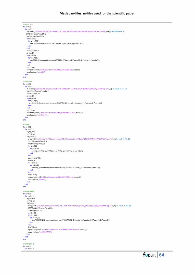
Matlab m-files: m-files used for the scientific paper

64

%% ARC 2.0 for y=0:10 for m=1:12 U=sprintf('C:\\Users\\Tim\\Documents\\TU Delft\\Afstuderen\\Data\\20%02d\\%02d\\ARCclip.tif',y,m); % result m-file 18 [ARC F6]=geotiffread(U); ARC2=zeros(500,300); for q=1:500 for w=1:300 ARC2(q,w)=(ARC(q,w)+ARC(q+1,w)+ARC(q,w+1)+ARC(q+1,w+1))/4; end end aantal=grid/0.1; A=size(B); for i=1:A(1); for j=1:A(2); aveARC(i,j)=nanmean(nanmean(ARC2((i-1)*aantal+1:i*aantal,(j-1)*aantal+1:j*aantal))); end end k=y*12+m; opslaan=sprintf('GridBlock\\Kaarten%02d\\ARC%03d.mat',maat,k); save(opslaan,'aveARC'); end end %% CHIRPS for y=0:10 for m=1:12 U=sprintf('C:\\Users\\Tim\\Documents\\TU Delft\\Afstuderen\\Data\\20%02d\\%02d\\CHIRPSclip.tif',y,m); % result m-file 18 [CHIRPS F7]=geotiffread(U); aantal=grid/0.05; A=size(B); for i=1:A(1); for j=1:A(2); aveCHIRPS(i,j)=nanmean(nanmean(CHIRPS((i-1)*aantal+1:i*aantal,(j-1)*aantal+1:j*aantal))); end end k=y*12+m; opslaan=sprintf('GridBlock\\Kaarten%02d\\CHIRPS%03d.mat',maat,k); save(opslaan,'aveCHIRPS'); end end %% RFE for y=0:10 for m=1:12 t=y*12+m; k=y*12+m; if T(5,t)==1; U=sprintf('C:\\Users\\Tim\\Documents\\TU Delft\\Afstuderen\\Data\\20%02d\\%02d\\FEWSNETclip.tif',y,m); % result m-file 18 [RFE F8]=geotiffread(U); RFE2=zeros(500,300); for q=1:500 for w=1:300 RFE2(q,w)=(RFE(q,w)+RFE(q+1,w)+RFE(q,w+1)+RFE(q+1,w+1))/4; end end aantal=grid/0.1; A=size(B); for i=1:A(1); for j=1:A(2); aveRFE(i,j)=nanmean(nanmean(RFE2((i-1)*aantal+1:i*aantal,(j-1)*aantal+1:j*aantal))); end end k=y*12+m; opslaan=sprintf('GridBlock\\Kaarten%02d\\RFE%03d.mat',maat,k); save(opslaan,'aveRFE'); end end end %% PERSIANN for y=0:10 for m=1:12 t=y*12+m; k=y*12+m; if T(4,t)==1; U=sprintf('C:\\Users\\Tim\\Documents\\TU Delft\\Afstuderen\\Data\\20%02d\\%02d\\PERSIANNclip.tif',y,m); % result m-file 18 [PERSIANN F9]=geotiffread(U); aantal=grid/0.25; A=size(B); for i=1:A(1); for j=1:A(2); avePERSIANN(i,j)=nanmean(nanmean(PERSIANN((i-1)*aantal+1:i*aantal,(j-1)*aantal+1:j*aantal))); end end k=y*12+m; opslaan=sprintf('GridBlock\\Kaarten%02d\\PERSIANN%03d.mat',maat,k); save(opslaan,'avePERSIANN'); end end end %% CMORPH for y=0:10 for m=1:12

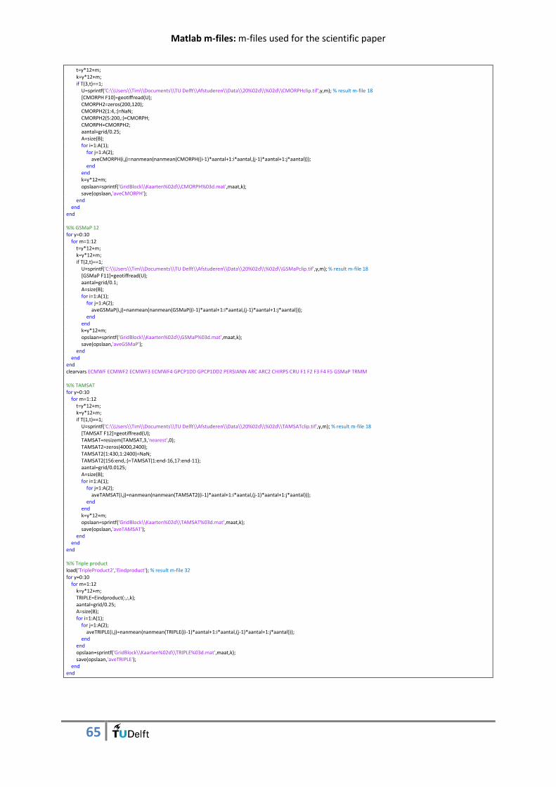
Matlab m-files: m-files used for the scientific paper

65

t=y*12+m; k=y*12+m; if T(3,t)==1; U=sprintf('C:\\Users\\Tim\\Documents\\TU Delft\\Afstuderen\\Data\\20%02d\\%02d\\CMORPHclip.tif',y,m); % result m-file 18 [CMORPH F10]=geotiffread(U); CMORPH2=zeros(200,120); CMORPH2(1:4,:)=NaN; CMORPH2(5:200,:)=CMORPH; CMORPH=CMORPH2; aantal=grid/0.25; A=size(B); for i=1:A(1); for j=1:A(2); aveCMORPH(i,j)=nanmean(nanmean(CMORPH((i-1)*aantal+1:i*aantal,(j-1)*aantal+1:j*aantal))); end end k=y*12+m; opslaan=sprintf('GridBlock\\Kaarten%02d\\CMORPH%03d.mat',maat,k); save(opslaan,'aveCMORPH'); end end end %% GSMaP 12 for y=0:10 for m=1:12 t=y*12+m; k=y*12+m; if T(2,t)==1; U=sprintf('C:\\Users\\Tim\\Documents\\TU Delft\\Afstuderen\\Data\\20%02d\\%02d\\GSMaPclip.tif',y,m); % result m-file 18 [GSMaP F11]=geotiffread(U); aantal=grid/0.1; A=size(B); for i=1:A(1); for j=1:A(2); aveGSMaP(i,j)=nanmean(nanmean(GSMaP((i-1)*aantal+1:i*aantal,(j-1)*aantal+1:j*aantal))); end end k=y*12+m; opslaan=sprintf('GridBlock\\Kaarten%02d\\GSMaP%03d.mat',maat,k); save(opslaan,'aveGSMaP'); end end end clearvars ECMWF ECMWF2 ECMWF3 ECMWF4 GPCP1DD GPCP1DD2 PERSIANN ARC ARC2 CHIRPS CRU F1 F2 F3 F4 F5 GSMaP TRMM %% TAMSAT for y=0:10 for m=1:12 t=y*12+m; k=y*12+m; if T(1,t)==1; U=sprintf('C:\\Users\\Tim\\Documents\\TU Delft\\Afstuderen\\Data\\20%02d\\%02d\\TAMSATclip.tif',y,m); % result m-file 18 [TAMSAT F12]=geotiffread(U); TAMSAT=resizem(TAMSAT,3,'nearest',0); TAMSAT2=zeros(4000,2400); TAMSAT2(1:430,1:2400)=NaN; TAMSAT2(156:end,:)=TAMSAT(1:end-16,17:end-11); aantal=grid/0.0125; A=size(B); for i=1:A(1); for j=1:A(2); aveTAMSAT(i,j)=nanmean(nanmean(TAMSAT2((i-1)*aantal+1:i*aantal,(j-1)*aantal+1:j*aantal))); end end k=y*12+m; opslaan=sprintf('GridBlock\\Kaarten%02d\\TAMSAT%03d.mat',maat,k); save(opslaan,'aveTAMSAT'); end end end %% Triple product load('TripleProduct2','Eindproduct'); % result m-file 32 for y=0:10 for m=1:12 k=y*12+m; TRIPLE=Eindproduct(:,:,k); aantal=grid/0.25; A=size(B); for i=1:A(1); for j=1:A(2); aveTRIPLE(i,j)=nanmean(nanmean(TRIPLE((i-1)*aantal+1:i*aantal,(j-1)*aantal+1:j*aantal))); end end opslaan=sprintf('GridBlock\\Kaarten%02d\\TRIPLE%03d.mat',maat,k); save(opslaan,'aveTRIPLE'); end end

Matlab m-files: m-files used for the scientific paper

66

4.2 Select pixels which are used for the validation Because for some pixel no ground measurements are located, the pixels are selected by using the

following m-file. This is done to make the calculations quicker and the possibility to calculate just a

particular area of the whole basin. So also a subbasin can be calculated. This map creates ones at

grids where a minimum of one ground measurements is located.

m-file 34 clear all close all clc size=0.25; % size selection, also done on 2.5 degrees tekst=['sennar ' ; 'rashad ' ; 'obied ' ; 'nyala ' ; 'nahoud ' ; 'madani ' ; 'kosti ' ; 'khar ' ; 'kasala ' ; 'kadugli ' ; 'atbara ' ; 'gadarf ' ; 'fasher ' ; 'duem ' ; 'damazine ' ; 'babanusa '; 'gondor ';'asswan '; 'cairo ';'luxor ';'qena ';'asyout ';'elminya ';'dangla ';'debretabor ';'addiszemen ';'ayikel '; 'adet ';'gorgora ';'enjibara ';'enfraz ';'wereta ';'zege ';'maksegnit ';'kidmaja ';'kimbaba ';'wetetabay ';'gundil ';'abayshelek ';'urana ';'wau ';'malakal ';'juba ';'yetemen ';'shindi ';'debremarcos';'teppi ';'masha ';'assosa ';'begi ';'sekela ';'motta ';'finote ';'gebeya ';'kitale ';'eldoret ';'kisumu ';'bukoba ';'musoma ';'mwanza ';'kigoma ';'kigali ']; teksttwee=['SENNAR.xls ' ; 'RASHAD.xls ' ; 'OBIED.xls ' ; 'NYALA.xls ' ; 'NAHOUD.xls ' ; 'MADANI.xls ' ; 'kosti.xls ' ; 'KHAR_RAIN.xls ' ; 'KASALA.xls ' ; 'KADUGLI.xls ' ; 'ATBARA.xls ' ; 'GADARF.xls ' ; 'FASHER.xls ' ; 'DUEM.xls ' ; 'DAMAZINE.xls ' ; 'BABANUSARAIN.xls'; 'GONDOR.xlsx '; 'ASSWAN.xlsx '; 'CAIRO.xlsx '; 'LUXOR.xlsx '; 'QENA.xlsx '; 'ASYOUT.xlsx '; 'ELMINYA.xlsx ';'DANGLA.xlsx '; 'DEBRETABOR.xlsx '; 'ADDISZEMEN.xlsx '; 'AYIKEL.xlsx '; 'ADET.xlsx '; 'GORGORA.xlsx ';'ENJIBARA.xlsx ';'ENFRAZ.xlsx '; 'WERETA.xlsx '; 'ZEGE.xlsx '; 'MAKSEGNIT.xlsx '; 'KIDMAJA.xlsx '; 'KIMBABA.xlsx '; 'WETETABAY.xlsx '; 'GUNDIL.xlsx '; 'ABAYSHELEKO.xlsx'; 'URANA.xlsx ';'WAU.xlsx ';'MALAKAL.xlsx ';'JUBA.xlsx '; 'YETEMEN.xlsx ';'SHINDI.xlsx ';'DEBREMARCOS.xlsx';'TEPPI.xlsx ';'MASHA.xlsx ';'ASSOSA.xlsx ';'BEGI.xlsx ';'SEKELA.xlsx ';'MOTTA.xlsx ';'FINOTE.xlsx ';'GEBEYA.xlsx ';'KITALE.xlsx ';'ELDORET.xlsx ';'KISUMU.xlsx ';'BUKOBA.xlsx ';'MUSOMA.xlsx ';'MWANZA.xlsx ';'KIGOMA.xlsx ';'KIGALI.xlsx ' ]; % excel with ground measurement data sizeblock=0.05; sizeblockarea=2.5; for xas=1:30/size; for yas=1:50/size; for j=0:10 for m=1:12; l=m+12*j; beginlon=20+(xas-1)*size; eindlon=20+(xas)*size; beginlat=40-(yas-1)*size; eindlat=40-(yas)*size; beginlonpunt=20+(xas-1)*size-sizeblockarea; eindlonpunt=20+(xas)*size+sizeblockarea; beginlatpunt=40-(yas-1)*size+sizeblockarea; eindlatpunt=40-(yas)*size-sizeblockarea; x1=linspace(beginlon+sizeblock/2,eindlon-sizeblock/2,size/sizeblock); y1=linspace(beginlat-sizeblock/2,eindlat+sizeblock/2,size/sizeblock); hoeveel=1; hoeveelpunt=1; for meting=1:62 Meting(1).Lat=13.33; Meting(1).Lon=33.37; Meting(1).Name='Sennar'; Meting(2).Lat=11.52; Meting(2).Lon=31.03; Meting(2).Name='Rashad'; Meting(3).Lat=13.10; Meting(3).Lon=30.14; Meting(3).Name='Obied'; Meting(4).Lat=12.03; Meting(4).Lon=24.53; Meting(4).Name='Nyala'; Meting(5).Lat=12.42; Meting(5).Lon=28.26; Meting(5).Name='Nahoud'; Meting(6).Lat=14.24; Meting(6).Lon=33.29; Meting(6).Name='Madini'; Meting(7).Lat=13.10; Meting(7).Lon=32.40; Meting(7).Name='Kosti'; Meting(8).Lat=15.6; Meting(8).Lon=32.549; Meting(8).Name='Khar'; Meting(9).Lat=15.28; Meting(9).Lon=36.24; Meting(9).Name='Kasala'; Meting(10).Lat=11; Meting(10).Lon=29.43; Meting(10).Name='Kadugli'; Meting(11).Lat=17.42; Meting(11).Lon=33.58; Meting(11).Name='Atbara'; Meting(12).Lat=14.02; Meting(12).Lon=35.24; Meting(12).Name='Gadarf'; Meting(13).Lat=13.37; Meting(13).Lon=25.20; Meting(13).Name='Fasher'; Meting(14).Lat=14; Meting(14).Lon=32.20; Meting(14).Name='Duem'; Meting(15).Lat=11.47; Meting(15).Lon=34.23; Meting(15).Name='Damazine'; Meting(16).Lat=11.20; Meting(16).Lon=27.49; Meting(16).Name='Babanusarai'; Meting(17).Lat=12.32; Meting(17).Lon=37.26; Meting(17).Name='Gondor'; Meting(18).Lat=23.58; Meting(18).Lon=32.47; Meting(18).Name='Asswan'; Meting(19).Lat=30.08; Meting(19).Lon=31.24; Meting(19).Name='Cairo'; Meting(20).Lat=25.40; Meting(20).Lon=32.42; Meting(20).Name='Luxor'; Meting(21).Lat=26.2; Meting(21).Lon=32.75; Meting(21).Name='Qena'; Meting(22).Lat=27.03; Meting(22).Lon=31.01; Meting(22).Name='Asyout'; Meting(23).Lat=28.05; Meting(23).Lon=30.44; Meting(23).Name='Elminya'; Meting(24).Lat=11.117; Meting(24).Lon=36.417; Meting(24).Name='Dangla'; Meting(25).Lat=11.883; Meting(25).Lon=38.033; Meting(25).Name='Debretabor'; Meting(26).Lat=12.117; Meting(26).Lon=37.867; Meting(26).Name='Addiszemen'; Meting(27).Lat=12.533; Meting(27).Lon=37.050; Meting(27).Name='Ayikel'; Meting(28).Lat=11.267; Meting(28).Lon=37.467; Meting(28).Name='Adet'; Meting(29).Lat=12.250; Meting(29).Lon=37.300; Meting(29).Name='Gorgora'; Meting(30).Lat=11.000; Meting(30).Lon=37.000; Meting(30).Name='Enjibara'; Meting(31).Lat=12.183; Meting(31).Lon=37.683; Meting(31).Name='Enfraz'; Meting(32).Lat=11.917; Meting(32).Lon=37.683; Meting(32).Name='Wereta'; Meting(33).Lat=11.683; Meting(33).Lon=37.317; Meting(33).Name='Zege'; Meting(34).Lat=12.367; Meting(34).Lon=37.550; Meting(34).Name='Maksegnit'; Meting(35).Lat=11.000; Meting(35).Lon=36.800; Meting(35).Name='Kidmaja'; Meting(36).Lat=11.550; Meting(36).Lon=37.380; Meting(36).Name='Kimbaba'; Meting(37).Lat=11.367; Meting(37).Lon=37.050; Meting(37).Name='Wetetabay'; Meting(38).Lat=10.950; Meting(38).Lon=37.070; Meting(38).Name='Gundil'; Meting(39).Lat=11.383; Meting(39).Lon=36.870; Meting(39).Name='AbaySheleko'; Meting(40).Lat=10.892; Meting(40).Lon=36.856; Meting(40).Name='Urana'; Meting(41).Lat=7.42; Meting(41).Lon=28.01; Meting(41).Name='Wau'; Meting(42).Lat=9.33; Meting(42).Lon=31.39; Meting(42).Name='Malakal'; Meting(43).Lat=4.52; Meting(43).Lon=31.36; Meting(43).Name='Juba';

Matlab m-files: m-files used for the scientific paper

67

Meting(44).Lat=10.33; Meting(44).Lon=38.13; Meting(44).Name='Yetemen'; Meting(45).Lat=10.43; Meting(45).Lon=36.57; Meting(45).Name='Shindi'; Meting(46).Lat=10.21; Meting(46).Lon=37.43; Meting(46).Name='Debremarcos'; Meting(47).Lat=7.2; Meting(47).Lon=35.42; Meting(47).Name='Teppi'; Meting(48).Lat=7.73; Meting(48).Lon=35.48; Meting(48).Name='Masha'; Meting(49).Lat=10.02; Meting(49).Lon=34.32; Meting(49).Name='Assosa'; Meting(50).Lat=9.35; Meting(50).Lon=34.53; Meting(50).Name='Begi'; Meting(51).Lat=11; Meting(51).Lon=37.13; Meting(51).Name='Sekela'; Meting(52).Lat=11.083; Meting(52).Lon=37.867; Meting(52).Name='Motta'; Meting(53).Lat=10.41; Meting(53).Lon=37.16; Meting(53).Name='Finote'; Meting(54).Lat=9.2; Meting(54).Lon=39.38; Meting(54).Name='Gebeya'; Meting(55).Lat=1.016; Meting(55).Lon=35; Meting(55).Name='Kitale'; Meting(56).Lat=0.405; Meting(56).Lon=35.224; Meting(56).Name='Eldoret'; Meting(57).Lat=-0.1; Meting(57).Lon=34.75; Meting(57).Name='Kisumu'; Meting(58).Lat=-1.333; Meting(58).Lon=31.817; Meting(58).Name='Bukoba'; Meting(59).Lat=-1.5; Meting(59).Lon=33.8; Meting(59).Name='Musoma'; Meting(60).Lat=-2.467; Meting(60).Lon=32.917; Meting(60).Name='Mwanza'; Meting(61).Lat=-4.88; Meting(61).Lon=29.63; Meting(61).Name='Kigoma'; Meting(62).Lat=-1.96; Meting(62).Lon=30.13; Meting(62).Name='Kigali'; if Meting(meting).Lat<=beginlat && Meting(meting).Lat>=eindlat && Meting(meting).Lon>=beginlon && Meting(meting).Lon<=eindlon IN(1:3,hoeveel)=[Meting(meting).Lat Meting(meting).Lon meting]; hoeveel=hoeveel+1; end if Meting(meting).Lat<=beginlatpunt && Meting(meting).Lat>=eindlatpunt && Meting(meting).Lon>=beginlonpunt && Meting(meting).Lon<=eindlonpunt INpunt(1:3,hoeveelpunt)=[Meting(meting).Lat Meting(meting).Lon meting]; hoeveelpunt=hoeveelpunt+1; end end if hoeveel>1 A=zeros(length(x1)); Coord=[]; if hoeveelpunt>1; i=1; P(xas,yas,l)=1; else P(xas,yas,l)=0; end else P(xas,yas,l)=0; end clearvars -except ResultZ Resultsigma j m xas yas size tekst teksttwee sizeblock l sizeblockarea end end end end save('GridBlock\Pixels025.mat','P');

A certain area is selected with the use of th following m-file.

m-file 35 clear all; close all; clc; %% selecting the pixel size and the area grid=2.5; method=sprintf('nearest'); %bicubic nearest or bilinear gebied=sprintf('C:\\Users\\Tim\\Documents\\TU Delft\\Afstuderen\\Data\\Layers\\sub\\bluenile'); % shapefile with the subbasins or basins % Nilebasin, albertnilebahraljabal, bahrelghazal, baroakobosobat, % bluenile,kagera, lakevictoria, lowerwhitenile, mainnile1, mainnile2, % mainnile3, mainnile4, semlikilalbert, sudd, tekezzeatbara or % victorianile %% make a mask of the selected area for the selected spatial resolution Nilebasin = shaperead(gebied,'UseGeoCoords',true); inLat=Nilebasin.Lat; inLon=Nilebasin.Lon; gridDensity=10; [inGrid,InRefVec]=vec2mtx(inLat,inLon,gridDensity); Masker=zeros(500,300); Mask = imfill(inGrid,'holes'); a1=floor(Nilebasin.BoundingBox(1,2)*10)/10-0.2; a2=floor(Nilebasin.BoundingBox(2,2)*10)/10+0.2; a3=floor(Nilebasin.BoundingBox(1,1)*10)/10-0.2; a4=floor(Nilebasin.BoundingBox(2,1)*10)/10+0.2; R1 = georasterref('RasterSize', size(Mask),'Latlim', [a1 a2], 'Lonlim', [a3 a4],'ColumnsStartFrom','south'); geoshow(Mask,R1,'DisplayType', 'Texturemap'); geoshow(Nilebasin.Lat,Nilebasin.Lon,'DisplayType','line','Color','k') grote=size(Mask); b1=grote(1)-1; b2=grote(2)-1; c1=(a1+10)*10+1; c2=(a3-20)*10+1; Masker(c1:c1+b1,c2:c2+b2)=Masker(c1:c1+b1,c2:c2+b2)+Mask; R2 = georasterref('RasterSize', size(Masker),'Latlim', [-10 40], 'Lonlim', [20 50],'ColumnsStartFrom','South'); geoshow(Masker,R2,'DisplayType', 'Texturemap'); geoshow(Nilebasin.Lat,Nilebasin.Lon,'DisplayType','line','Color','k') Gebied=zeros(50/grid,30/grid); aantal=grid/0.1; A=size(Gebied); for i=1:A(1); for j=1:A(2); aveMasker(i,j)=nanmean(nanmean(Masker((i-1)*aantal+1:i*aantal,(j-1)*aantal+1:j*aantal))); if aveMasker(i,j)>0; Gebiedtot(i,j)=1;

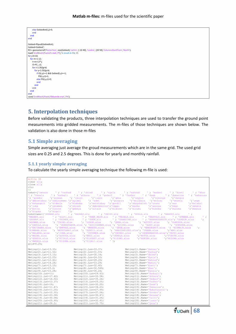
Matlab m-files: m-files used for the scientific paper

68

else Gebiedtot(i,j)=0; end end end Gebied=flipud(Gebiedtot); Gebied=Gebied'; R3 = georasterref('RasterSize', size(Gebied),'Latlim', [-10 40], 'Lonlim', [20 50],'ColumnsStartFrom','North'); load('GridBlock\Pixels25.mat','P'); % result m-file 35 for j=0:10; for m=1:12; t=m+12*j; O=P(:,:,t); for i=1:30/grid; for y=1:50/grid; if O(i,y)==1 && Gebied(i,y)==1; PX(i,y,t)=1; else PX(i,y,t)=0; end end end end end save('GridBlock\Pixels25bluenile.mat','PX');

5. Interpolation techniques Before validating the products, three interpolation techniques are used to transfer the ground point

measurements into gridded measurements. The m-files of those techniques are shown below. The

validation is also done in those m-files

5.1 Simple averaging Simple averaging just average the groud measurements which are in the same grid. The used grid

sizes are 0.25 and 2.5 degrees. This is done for yearly and monthly rainfall.

5.1.1 yearly simple averaging

To calculate the yearly simple averaging technique the following m-file is used:

m-file 36

clear all;

close all;

clc;

%%

tekst=['sennar ' ; 'rashad ' ; 'obied ' ; 'nyala ' ; 'nahoud ' ; 'madani ' ; 'kosti ' ; 'khar

' ; 'kasala ' ; 'kadugli ' ; 'atbara ' ; 'gadarf ' ; 'fasher ' ; 'duem ' ; 'damazine ' ; 'babanusa

'; 'gondor ';'asswan '; 'cairo ';'luxor ';'qena ';'asyout ';'elminya ';'dangla

';'debretabor ';'addiszemen ';'ayikel '; 'adet ';'gorgora ';'enjibara ';'enfraz ';'wereta ';'zege

';'maksegnit ';'kidmaja ';'kimbaba ';'wetetabay ';'gundil ';'abayshelek ';'urana ';'wau ';'malakal

';'juba ';'yetemen ';'shindi ';'debremarcos';'teppi ';'masha ';'assosa ';'begi ';'sekela

';'motta ';'finote ';'gebeya ';'kitale ';'eldoret ';'kisumu ';'bukoba ';'musoma ';'mwanza

';'kigoma ';'kigali '];

teksttwee=['SENNAR.xls ' ; 'RASHAD.xls ' ; 'OBIED.xls ' ; 'NYALA.xls ' ; 'NAHOUD.xls ' ;

'MADANI.xls ' ; 'kosti.xls ' ; 'KHAR_RAIN.xls ' ; 'KASALA.xls ' ; 'KADUGLI.xls ' ; 'ATBARA.xls ' ;

'GADARF.xls ' ; 'FASHER.xls ' ; 'DUEM.xls ' ; 'DAMAZINE.xls ' ; 'BABANUSARAIN.xls'; 'GONDOR.xlsx ';

'ASSWAN.xlsx '; 'CAIRO.xlsx '; 'LUXOR.xlsx '; 'QENA.xlsx '; 'ASYOUT.xlsx '; 'ELMINYA.xlsx

';'DANGLA.xlsx '; 'DEBRETABOR.xlsx '; 'ADDISZEMEN.xlsx '; 'AYIKEL.xlsx '; 'ADET.xlsx '; 'GORGORA.xlsx

';'ENJIBARA.xlsx ';'ENFRAZ.xlsx '; 'WERETA.xlsx '; 'ZEGE.xlsx '; 'MAKSEGNIT.xlsx '; 'KIDMAJA.xlsx ';

'KIMBABA.xlsx '; 'WETETABAY.xlsx '; 'GUNDIL.xlsx '; 'ABAYSHELEKO.xlsx'; 'URANA.xlsx ';'WAU.xlsx

';'MALAKAL.xlsx ';'JUBA.xlsx '; 'YETEMEN.xlsx ';'SHINDI.xlsx ';'DEBREMARCOS.xlsx';'TEPPI.xlsx

';'MASHA.xlsx ';'ASSOSA.xlsx ';'BEGI.xlsx ';'SEKELA.xlsx ';'MOTTA.xlsx ';'FINOTE.xlsx

';'GEBEYA.xlsx ';'KITALE.xlsx ';'ELDORET.xlsx ';'KISUMU.xlsx ';'BUKOBA.xlsx ';'MUSOMA.xlsx

';'MWANZA.xlsx ';'KIGOMA.xlsx ';'KIGALI.xlsx ' ];

grid=0.25;

Meting(1).Lat=13.33; Meting(1).Lon=33.37; Meting(1).Name='Sennar';

Meting(2).Lat=11.52; Meting(2).Lon=31.03; Meting(2).Name='Rashad';

Meting(3).Lat=13.10; Meting(3).Lon=30.14; Meting(3).Name='Obied';

Meting(4).Lat=12.03; Meting(4).Lon=24.53; Meting(4).Name='Nyala';

Meting(5).Lat=12.42; Meting(5).Lon=28.26; Meting(5).Name='Nahoud';

Meting(6).Lat=14.24; Meting(6).Lon=33.29; Meting(6).Name='Madini';

Meting(7).Lat=13.10; Meting(7).Lon=32.40; Meting(7).Name='Kosti';

Meting(8).Lat=15.6; Meting(8).Lon=32.549; Meting(8).Name='Khar';

Meting(9).Lat=15.28; Meting(9).Lon=36.24; Meting(9).Name='Kasala';

Meting(10).Lat=11; Meting(10).Lon=29.43; Meting(10).Name='Kadugli';

Meting(11).Lat=17.42; Meting(11).Lon=33.58; Meting(11).Name='Atbara';

Meting(12).Lat=14.02; Meting(12).Lon=35.24; Meting(12).Name='Gadarf';

Meting(13).Lat=13.37; Meting(13).Lon=25.20; Meting(13).Name='Fasher';

Meting(14).Lat=14; Meting(14).Lon=32.20; Meting(14).Name='Duem';

Meting(15).Lat=11.47; Meting(15).Lon=34.23; Meting(15).Name='Damazine';

Meting(16).Lat=11.20; Meting(16).Lon=27.49; Meting(16).Name='Babanusarai';

Meting(17).Lat=12.32; Meting(17).Lon=37.26; Meting(17).Name='Gondor';

Meting(18).Lat=23.58; Meting(18).Lon=32.47; Meting(18).Name='Asswan';

Meting(19).Lat=30.08; Meting(19).Lon=31.24; Meting(19).Name='Cairo';

Meting(20).Lat=25.40; Meting(20).Lon=32.42; Meting(20).Name='Luxor';

Meting(21).Lat=26.2; Meting(21).Lon=32.75; Meting(21).Name='Qena';

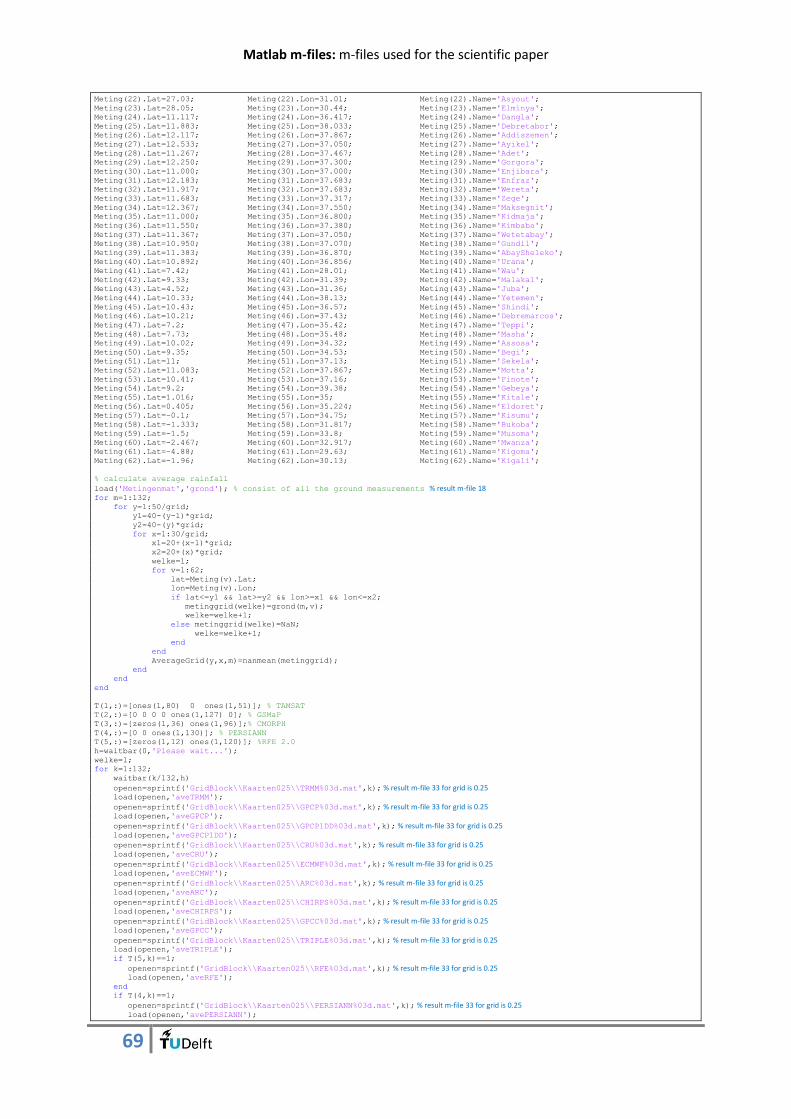
Matlab m-files: m-files used for the scientific paper

69

Meting(22).Lat=27.03; Meting(22).Lon=31.01; Meting(22).Name='Asyout';

Meting(23).Lat=28.05; Meting(23).Lon=30.44; Meting(23).Name='Elminya';

Meting(24).Lat=11.117; Meting(24).Lon=36.417; Meting(24).Name='Dangla';

Meting(25).Lat=11.883; Meting(25).Lon=38.033; Meting(25).Name='Debretabor';

Meting(26).Lat=12.117; Meting(26).Lon=37.867; Meting(26).Name='Addiszemen';

Meting(27).Lat=12.533; Meting(27).Lon=37.050; Meting(27).Name='Ayikel';

Meting(28).Lat=11.267; Meting(28).Lon=37.467; Meting(28).Name='Adet';

Meting(29).Lat=12.250; Meting(29).Lon=37.300; Meting(29).Name='Gorgora';

Meting(30).Lat=11.000; Meting(30).Lon=37.000; Meting(30).Name='Enjibara';

Meting(31).Lat=12.183; Meting(31).Lon=37.683; Meting(31).Name='Enfraz';

Meting(32).Lat=11.917; Meting(32).Lon=37.683; Meting(32).Name='Wereta';

Meting(33).Lat=11.683; Meting(33).Lon=37.317; Meting(33).Name='Zege';

Meting(34).Lat=12.367; Meting(34).Lon=37.550; Meting(34).Name='Maksegnit';

Meting(35).Lat=11.000; Meting(35).Lon=36.800; Meting(35).Name='Kidmaja';

Meting(36).Lat=11.550; Meting(36).Lon=37.380; Meting(36).Name='Kimbaba';

Meting(37).Lat=11.367; Meting(37).Lon=37.050; Meting(37).Name='Wetetabay';

Meting(38).Lat=10.950; Meting(38).Lon=37.070; Meting(38).Name='Gundil';

Meting(39).Lat=11.383; Meting(39).Lon=36.870; Meting(39).Name='AbaySheleko';

Meting(40).Lat=10.892; Meting(40).Lon=36.856; Meting(40).Name='Urana';

Meting(41).Lat=7.42; Meting(41).Lon=28.01; Meting(41).Name='Wau';

Meting(42).Lat=9.33; Meting(42).Lon=31.39; Meting(42).Name='Malakal';

Meting(43).Lat=4.52; Meting(43).Lon=31.36; Meting(43).Name='Juba';

Meting(44).Lat=10.33; Meting(44).Lon=38.13; Meting(44).Name='Yetemen';

Meting(45).Lat=10.43; Meting(45).Lon=36.57; Meting(45).Name='Shindi';

Meting(46).Lat=10.21; Meting(46).Lon=37.43; Meting(46).Name='Debremarcos';

Meting(47).Lat=7.2; Meting(47).Lon=35.42; Meting(47).Name='Teppi';

Meting(48).Lat=7.73; Meting(48).Lon=35.48; Meting(48).Name='Masha';

Meting(49).Lat=10.02; Meting(49).Lon=34.32; Meting(49).Name='Assosa';

Meting(50).Lat=9.35; Meting(50).Lon=34.53; Meting(50).Name='Begi';

Meting(51).Lat=11; Meting(51).Lon=37.13; Meting(51).Name='Sekela';

Meting(52).Lat=11.083; Meting(52).Lon=37.867; Meting(52).Name='Motta';

Meting(53).Lat=10.41; Meting(53).Lon=37.16; Meting(53).Name='Finote';

Meting(54).Lat=9.2; Meting(54).Lon=39.38; Meting(54).Name='Gebeya';

Meting(55).Lat=1.016; Meting(55).Lon=35; Meting(55).Name='Kitale';

Meting(56).Lat=0.405; Meting(56).Lon=35.224; Meting(56).Name='Eldoret';

Meting(57).Lat=-0.1; Meting(57).Lon=34.75; Meting(57).Name='Kisumu';

Meting(58).Lat=-1.333; Meting(58).Lon=31.817; Meting(58).Name='Bukoba';

Meting(59).Lat=-1.5; Meting(59).Lon=33.8; Meting(59).Name='Musoma';

Meting(60).Lat=-2.467; Meting(60).Lon=32.917; Meting(60).Name='Mwanza';

Meting(61).Lat=-4.88; Meting(61).Lon=29.63; Meting(61).Name='Kigoma';

Meting(62).Lat=-1.96; Meting(62).Lon=30.13; Meting(62).Name='Kigali';

% calculate average rainfall

load('Metingenmat','grond'); % consist of all the ground measurements % result m-file 18 for m=1:132;

for y=1:50/grid;

y1=40-(y-1)*grid;

y2=40-(y)*grid;

for x=1:30/grid;

x1=20+(x-1)*grid;

x2=20+(x)*grid;

welke=1;

for v=1:62;

lat=Meting(v).Lat;

lon=Meting(v).Lon;

if lat<=y1 && lat>=y2 && lon>=x1 && lon<=x2;

metinggrid(welke)=grond(m,v);

welke=welke+1;

else metinggrid(welke)=NaN;

welke=welke+1;

end

end

AverageGrid(y,x,m)=nanmean(metinggrid);

end

end

end

T(1,:)=[ones(1,80) 0 ones(1,51)]; % TAMSAT

T(2,:)=[0 0 0 0 ones(1,127) 0]; % GSMaP

T(3,:)=[zeros(1,36) ones(1,96)];% CMORPH

T(4,:)=[0 0 ones(1,130)]; % PERSIANN

T(5,:)=[zeros(1,12) ones(1,120)]; %RFE 2.0

h=waitbar(0,'Please wait...');

welke=1;

for k=1:132;

waitbar(k/132,h)

openen=sprintf('GridBlock\\Kaarten025\\TRMM%03d.mat',k); % result m-file 33 for grid is 0.25 load(openen,'aveTRMM');

openen=sprintf('GridBlock\\Kaarten025\\GPCP%03d.mat',k); % result m-file 33 for grid is 0.25 load(openen,'aveGPCP');

openen=sprintf('GridBlock\\Kaarten025\\GPCP1DD%03d.mat',k); % result m-file 33 for grid is 0.25 load(openen,'aveGPCP1DD');

openen=sprintf('GridBlock\\Kaarten025\\CRU%03d.mat',k); % result m-file 33 for grid is 0.25 load(openen,'aveCRU');

openen=sprintf('GridBlock\\Kaarten025\\ECMWF%03d.mat',k); % result m-file 33 for grid is 0.25 load(openen,'aveECMWF');

openen=sprintf('GridBlock\\Kaarten025\\ARC%03d.mat',k); % result m-file 33 for grid is 0.25 load(openen,'aveARC');

openen=sprintf('GridBlock\\Kaarten025\\CHIRPS%03d.mat',k); % result m-file 33 for grid is 0.25 load(openen,'aveCHIRPS');

openen=sprintf('GridBlock\\Kaarten025\\GPCC%03d.mat',k); % result m-file 33 for grid is 0.25 load(openen,'aveGPCC');

openen=sprintf('GridBlock\\Kaarten025\\TRIPLE%03d.mat',k); % result m-file 33 for grid is 0.25 load(openen,'aveTRIPLE');

if T(5,k)==1;

openen=sprintf('GridBlock\\Kaarten025\\RFE%03d.mat',k); % result m-file 33 for grid is 0.25 load(openen,'aveRFE');

end

if T(4,k)==1;

openen=sprintf('GridBlock\\Kaarten025\\PERSIANN%03d.mat',k); % result m-file 33 for grid is 0.25 load(openen,'avePERSIANN');

Matlab m-files: m-files used for the scientific paper

70

end

if T(3,k)==1;

openen=sprintf('GridBlock\\Kaarten025\\CMORPH%03d.mat',k); % result m-file 33 for grid is 0.25 load(openen,'aveCMORPH');

end

if T(2,k)==1;

openen=sprintf('GridBlock\\Kaarten025\\GSMaP%03d.mat',k); % result m-file 33 for grid is 0.25 load(openen,'aveGSMaP');

end

if T(1,k)==1;

openen=sprintf('GridBlock\\Kaarten025\\TAMSAT%03d.mat',k); % result m-file 33 for grid is 0.25 load(openen,'aveTAMSAT');

end

% load('GridBlock\Pixels25bluenile.mat','PX'); %PX for subbasin

% K=PX;%PX for subbasin

% PX=0;%PX for subbasin

load('GridBlock\Pixels025.mat','P') % result m-file 35 K=P;

K=permute(K,[2 1 3]);

P=0;

for i=1:50/grid;

for j=1:30/grid;

if K(i,j,k)==1;

Vergelijken(1,welke)=AverageGrid(i,j,k);

Vergelijken(2,welke)=aveTRMM(i,j);

Vergelijken(3,welke)=aveGPCP(i,j);

Vergelijken(4,welke)=aveGPCP1DD(i,j);

Vergelijken(5,welke)=aveCRU(i,j);

Vergelijken(6,welke)=aveECMWF(i,j);

Vergelijken(7,welke)=aveARC(i,j);

Vergelijken(8,welke)=aveCHIRPS(i,j);

Vergelijken(14,welke)=aveGPCC(i,j);

Vergelijken(15,welke)=aveTRIPLE(i,j);

Vergelijken(16,welke)=max(Vergelijken(2:14,welke));

if T(5,k)==1;

Vergelijken(9,welke)=aveRFE(i,j);

else Vergelijken(9,welke)=NaN;

end

if T(4,k)==1;

Vergelijken(10,welke)=avePERSIANN(i,j);

else Vergelijken(10,welke)=NaN;

end

if T(3,k)==1;

Vergelijken(11,welke)=aveCMORPH(i,j);

else Vergelijken(11,welke)=NaN;

end

if T(2,k)==1;

Vergelijken(12,welke)=aveGSMaP(i,j);

else Vergelijken(12,welke)=NaN;

end

if T(1,k)==1;

Vergelijken(13,welke)=aveTAMSAT(i,j);

else Vergelijken(13,welke)=NaN;

end

welke=welke+1;

end

end

end

end

tekst3=['TRMM ';'GPCP ';'GPCP1DD ';'CRU ';'ECMWF ';'ARC ';'CHIRPS ';'RFE ';'PERSIANN';'CMORPH ';'GSMaP

';'TAMSAT ';'GPCC ';'TRIPLE '];

letters=[4 4 7 3 5 3 6 3 8 6 5 6 4 6];

for welkproduct=1:15;

Vergelijktwee=[];

Vergelijktwee(1,:)=Vergelijken(1,:);

Vergelijktwee(2,:)=Vergelijken((welkproduct+1),:);

for i=1:length(Vergelijktwee);

if Vergelijktwee(1,i)<=0;

Vergelijktwee(1,i)=NaN;

end

end

for i=1:length(Vergelijktwee);

if Vergelijktwee(2,i)<=0;

Vergelijktwee(2,i)=NaN;

end

end

Vergelijktwee=Vergelijktwee(:,all(~isnan(Vergelijktwee)));

for i=1:length(Vergelijktwee);

if Vergelijktwee(1,i)<=0;

Vergelijktwee(1,i)=NaN;

end

end

Grond=Vergelijktwee(1,:);

Product=Vergelijktwee(2,:);

gemGrond=nanmean(Grond);

gemProduct=nanmean(Product);

sumGrond=sum(Grond);

sumProduct=sum(Product);

boven=sum((Grond-gemGrond).*(Product-gemProduct));

onder=sqrt(sum((Grond-gemGrond).^2))*sqrt(sum((Product-gemProduct).^2));

Corr(welkproduct)=boven/onder;

Verschil=Product-Grond;

Bias(welkproduct)=sum(Verschil)/length(Vergelijktwee);

Bias2(welkproduct)=sumProduct/sumGrond;

RMSE(welkproduct)=100*sqrt(nanmean(Verschil.^2))/gemGrond;

end

%% make scatter figure

welkproduct=10; %fill in the product 1=TRMM 2=GPCP 3=GPCP1DD 4=CRU 5=ECMWF 6=ARC 7=CHIRPS 8=RFE 9=PERSIANN 10=CMORPH 11=GSMaP

12=TAMSAT 13=GPCC 14=TRIPLE

Matlab m-files: m-files used for the scientific paper

71

figure(1);

Vergelijktwee=[];

Vergelijktwee(1,:)=Vergelijken(1,:);

Vergelijktwee(2,:)=Vergelijken((welkproduct+1),:);

for i=1:length(Vergelijktwee);

if Vergelijktwee(1,i)<=0;

Vergelijktwee(1,i)=NaN;

end

end

for i=1:length(Vergelijktwee);

if Vergelijktwee(2,i)<=0;

Vergelijktwee(2,i)=NaN;

end

end

Vergelijktwee=Vergelijktwee(:,all(~isnan(Vergelijktwee)));

for i=1:length(Vergelijktwee);

if Vergelijktwee(1,i)<=0;

Vergelijktwee(1,i)=NaN;

end

end

Grond=Vergelijktwee(1,:);

Product=Vergelijktwee(2,:);

plot(1:10,1:10);

hold on;

plot(1:6,1:6);

h=legend('test ','test2 ','Location','NorthWest')

handle = get(h);

close(figure(1));

p=figure(2);

p=figure('units','normalized','outerposition',[0 0 1 1]);

hold on;

str={sprintf('Corr = %0.03f',Corr(welkproduct)),sprintf('RMSE =

%0.2f',RMSE(welkproduct)),sprintf('Bias=%0.2f',Bias(welkproduct))};

fw=@(x) x;

fplot(fw,[0 max(Product)],'c--');

hold on

plot(Grond,Product,'.');

xlabel('Ground Measurement');

ylabel('Product Estimation');

annotation('textbox',handle.UserData.LegendPosition,'String',str,'EdgeColor','none');

titel=sprintf('%s Nile Basin 2.5 degree',tekst3(welkproduct,1:letters(welkproduct)));

title(titel);

5.1.2 Monthly simple averaging

To calculate the monthly simple averaging technique the following m-file is used:

m-file 37 clear all; close all; clc; grid=2.5; % grid 0.25 degrees getal=25; % 025 if 0.25 degrees is done %% tekst=['sennar ' ; 'rashad ' ; 'obied ' ; 'nyala ' ; 'nahoud ' ; 'madani ' ; 'kosti ' ; 'khar ' ; 'kasala ' ; 'kadugli ' ; 'atbara ' ; 'gadarf ' ; 'fasher ' ; 'duem ' ; 'damazine ' ; 'babanusa '; 'gondor ';'asswan '; 'cairo ';'luxor ';'qena ';'asyout ';'elminya ';'dangla ';'debretabor ';'addiszemen ';'ayikel '; 'adet ';'gorgora ';'enjibara ';'enfraz ';'wereta ';'zege ';'maksegnit ';'kidmaja ';'kimbaba ';'wetetabay ';'gundil ';'abayshelek ';'urana ';'wau ';'malakal ';'juba ';'yetemen ';'shindi ';'debremarcos';'teppi ';'masha ';'assosa ';'begi ';'sekela ';'motta ';'finote ';'gebeya ';'kitale ';'eldoret ';'kisumu ';'bukoba ';'musoma ';'mwanza ';'kigoma ';'kigali ']; teksttwee=['SENNAR.xls ' ; 'RASHAD.xls ' ; 'OBIED.xls ' ; 'NYALA.xls ' ; 'NAHOUD.xls ' ; 'MADANI.xls ' ; 'kosti.xls ' ; 'KHAR_RAIN.xls ' ; 'KASALA.xls ' ; 'KADUGLI.xls ' ; 'ATBARA.xls ' ; 'GADARF.xls ' ; 'FASHER.xls ' ; 'DUEM.xls ' ; 'DAMAZINE.xls ' ; 'BABANUSARAIN.xls'; 'GONDOR.xlsx '; 'ASSWAN.xlsx '; 'CAIRO.xlsx '; 'LUXOR.xlsx '; 'QENA.xlsx '; 'ASYOUT.xlsx '; 'ELMINYA.xlsx ';'DANGLA.xlsx '; 'DEBRETABOR.xlsx '; 'ADDISZEMEN.xlsx '; 'AYIKEL.xlsx '; 'ADET.xlsx '; 'GORGORA.xlsx ';'ENJIBARA.xlsx ';'ENFRAZ.xlsx '; 'WERETA.xlsx '; 'ZEGE.xlsx '; 'MAKSEGNIT.xlsx '; 'KIDMAJA.xlsx '; 'KIMBABA.xlsx '; 'WETETABAY.xlsx '; 'GUNDIL.xlsx '; 'ABAYSHELEKO.xlsx'; 'URANA.xlsx ';'WAU.xlsx ';'MALAKAL.xlsx ';'JUBA.xlsx '; 'YETEMEN.xlsx ';'SHINDI.xlsx ';'DEBREMARCOS.xlsx';'TEPPI.xlsx ';'MASHA.xlsx ';'ASSOSA.xlsx ';'BEGI.xlsx ';'SEKELA.xlsx ';'MOTTA.xlsx ';'FINOTE.xlsx ';'GEBEYA.xlsx ';'KITALE.xlsx ';'ELDORET.xlsx ';'KISUMU.xlsx ';'BUKOBA.xlsx ';'MUSOMA.xlsx ';'MWANZA.xlsx ';'KIGOMA.xlsx ';'KIGALI.xlsx ' ]; Meting(1).Lat=13.33; Meting(1).Lon=33.37; Meting(1).Name='Sennar'; Meting(2).Lat=11.52; Meting(2).Lon=31.03; Meting(2).Name='Rashad'; Meting(3).Lat=13.10; Meting(3).Lon=30.14; Meting(3).Name='Obied'; Meting(4).Lat=12.03; Meting(4).Lon=24.53; Meting(4).Name='Nyala'; Meting(5).Lat=12.42; Meting(5).Lon=28.26; Meting(5).Name='Nahoud'; Meting(6).Lat=14.24; Meting(6).Lon=33.29; Meting(6).Name='Madini'; Meting(7).Lat=13.10; Meting(7).Lon=32.40; Meting(7).Name='Kosti'; Meting(8).Lat=15.6; Meting(8).Lon=32.549; Meting(8).Name='Khar'; Meting(9).Lat=15.28; Meting(9).Lon=36.24; Meting(9).Name='Kasala'; Meting(10).Lat=11; Meting(10).Lon=29.43; Meting(10).Name='Kadugli'; Meting(11).Lat=17.42; Meting(11).Lon=33.58; Meting(11).Name='Atbara'; Meting(12).Lat=14.02; Meting(12).Lon=35.24; Meting(12).Name='Gadarf'; Meting(13).Lat=13.37; Meting(13).Lon=25.20; Meting(13).Name='Fasher'; Meting(14).Lat=14; Meting(14).Lon=32.20; Meting(14).Name='Duem'; Meting(15).Lat=11.47; Meting(15).Lon=34.23; Meting(15).Name='Damazine'; Meting(16).Lat=11.20; Meting(16).Lon=27.49; Meting(16).Name='Babanusarai'; Meting(17).Lat=12.32; Meting(17).Lon=37.26; Meting(17).Name='Gondor'; Meting(18).Lat=23.58; Meting(18).Lon=32.47; Meting(18).Name='Asswan'; Meting(19).Lat=30.08; Meting(19).Lon=31.24; Meting(19).Name='Cairo'; Meting(20).Lat=25.40; Meting(20).Lon=32.42; Meting(20).Name='Luxor'; Meting(21).Lat=26.2; Meting(21).Lon=32.75; Meting(21).Name='Qena'; Meting(22).Lat=27.03; Meting(22).Lon=31.01; Meting(22).Name='Asyout'; Meting(23).Lat=28.05; Meting(23).Lon=30.44; Meting(23).Name='Elminya'; Meting(24).Lat=11.117; Meting(24).Lon=36.417; Meting(24).Name='Dangla'; Meting(25).Lat=11.883; Meting(25).Lon=38.033; Meting(25).Name='Debretabor'; Meting(26).Lat=12.117; Meting(26).Lon=37.867; Meting(26).Name='Addiszemen';

Matlab m-files: m-files used for the scientific paper

72

Meting(27).Lat=12.533; Meting(27).Lon=37.050; Meting(27).Name='Ayikel'; Meting(28).Lat=11.267; Meting(28).Lon=37.467; Meting(28).Name='Adet'; Meting(29).Lat=12.250; Meting(29).Lon=37.300; Meting(29).Name='Gorgora'; Meting(30).Lat=11.000; Meting(30).Lon=37.000; Meting(30).Name='Enjibara'; Meting(31).Lat=12.183; Meting(31).Lon=37.683; Meting(31).Name='Enfraz'; Meting(32).Lat=11.917; Meting(32).Lon=37.683; Meting(32).Name='Wereta'; Meting(33).Lat=11.683; Meting(33).Lon=37.317; Meting(33).Name='Zege'; Meting(34).Lat=12.367; Meting(34).Lon=37.550; Meting(34).Name='Maksegnit'; Meting(35).Lat=11.000; Meting(35).Lon=36.800; Meting(35).Name='Kidmaja'; Meting(36).Lat=11.550; Meting(36).Lon=37.380; Meting(36).Name='Kimbaba'; Meting(37).Lat=11.367; Meting(37).Lon=37.050; Meting(37).Name='Wetetabay'; Meting(38).Lat=10.950; Meting(38).Lon=37.070; Meting(38).Name='Gundil'; Meting(39).Lat=11.383; Meting(39).Lon=36.870; Meting(39).Name='AbaySheleko'; Meting(40).Lat=10.892; Meting(40).Lon=36.856; Meting(40).Name='Urana'; Meting(41).Lat=7.42; Meting(41).Lon=28.01; Meting(41).Name='Wau'; Meting(42).Lat=9.33; Meting(42).Lon=31.39; Meting(42).Name='Malakal'; Meting(43).Lat=4.52; Meting(43).Lon=31.36; Meting(43).Name='Juba'; Meting(44).Lat=10.33; Meting(44).Lon=38.13; Meting(44).Name='Yetemen'; Meting(45).Lat=10.43; Meting(45).Lon=36.57; Meting(45).Name='Shindi'; Meting(46).Lat=10.21; Meting(46).Lon=37.43; Meting(46).Name='Debremarcos'; Meting(47).Lat=7.2; Meting(47).Lon=35.42; Meting(47).Name='Teppi'; Meting(48).Lat=7.73; Meting(48).Lon=35.48; Meting(48).Name='Masha'; Meting(49).Lat=10.02; Meting(49).Lon=34.32; Meting(49).Name='Assosa'; Meting(50).Lat=9.35; Meting(50).Lon=34.53; Meting(50).Name='Begi'; Meting(51).Lat=11; Meting(51).Lon=37.13; Meting(51).Name='Sekela'; Meting(52).Lat=11.083; Meting(52).Lon=37.867; Meting(52).Name='Motta'; Meting(53).Lat=10.41; Meting(53).Lon=37.16; Meting(53).Name='Finote'; Meting(54).Lat=9.2; Meting(54).Lon=39.38; Meting(54).Name='Gebeya'; Meting(55).Lat=1.016; Meting(55).Lon=35; Meting(55).Name='Kitale'; Meting(56).Lat=0.405; Meting(56).Lon=35.224; Meting(56).Name='Eldoret'; Meting(57).Lat=-0.1; Meting(57).Lon=34.75; Meting(57).Name='Kisumu'; Meting(58).Lat=-1.333; Meting(58).Lon=31.817; Meting(58).Name='Bukoba'; Meting(59).Lat=-1.5; Meting(59).Lon=33.8; Meting(59).Name='Musoma'; Meting(60).Lat=-2.467; Meting(60).Lon=32.917; Meting(60).Name='Mwanza'; Meting(61).Lat=-4.88; Meting(61).Lon=29.63; Meting(61).Name='Kigoma'; Meting(62).Lat=-1.96; Meting(62).Lon=30.13; Meting(62).Name='Kigali'; %% load('Metingenmat','grond'); % result m-file 26 for j=0:10; for v=1:62; grondjaar(j+1,v)=nanmean(grond(j*12+1:j*12+12,v))*12; end end for j=0:10; k=j+1; aantal(k)=1; for v=1:62; bi=isnan(grondjaar(k,v)); if bi==0; doen(k,aantal(k))=v; aantal(k)=aantal(k)+1; end end end %% for j=0:10; for k=1:12; m=k+j*12; for y=1:50/grid; y1=40-(y-1)*grid; y2=40-(y)*grid; for x=1:30/grid; x1=20+(x-1)*grid; x2=20+(x)*grid; welke=1; for v=1:62; lat=Meting(v).Lat; lon=Meting(v).Lon; if lat<=y1 && lat>=y2 && lon>=x1 && lon<=x2; metinggrid(welke)=grondjaar(j+1,v); welke=welke+1; else metinggrid(welke)=NaN; welke=welke+1; end end AverageGrid(y,x,j+1)=nanmean(metinggrid); end end end end %% % T(1,:)=[ones(1,80) 0 ones(1,51)]; % TAMSAT % T(2,:)=[0 0 0 0 ones(1,127) 0]; % GSMaP % T(3,:)=[zeros(1,36) ones(1,96)];% CMORPH % T(4,:)=[0 0 ones(1,130)]; % PERSIANN % T(5,:)=[zeros(1,12) ones(1,120)]; %RFE 2.0 T(1,:)=[1 1 1 1 1 1 0 1 1 1 1]; % TAMSAT T(2,:)=[0 1 1 1 1 1 1 1 1 1 0]; % GSMaP T(3,:)=[0 0 0 1 1 1 1 1 1 1 1];% CMORPH T(4,:)=[0 1 1 1 1 1 1 1 1 1 1]; % PERSIANN T(5,:)=[0 1 1 1 1 1 1 1 1 1 1]; %RFE 2.0 h=waitbar(0,'Please wait...'); welke=1; %%

Matlab m-files: m-files used for the scientific paper

73

for j=1:11; for m=1:12; k=12*(j-1)+m; waitbar(j/11,h) openen=sprintf('GridBlock\\Kaarten%02d\\TRMM%03d.mat',getal,k); % result m-file 33 for grid is 0.25 load(openen,'aveTRMM'); T1(k,:,:)=aveTRMM; openen=sprintf('GridBlock\\Kaarten%02d\\GPCP%03d.mat',getal,k); % result m-file 33 for grid is 0.25 load(openen,'aveGPCP'); T2(k,:,:)=aveGPCP; openen=sprintf('GridBlock\\Kaarten%02d\\GPCP1DD%03d.mat',getal,k); % result m-file 33 for grid is 0.25 load(openen,'aveGPCP1DD'); T3(k,:,:)=aveGPCP1DD; openen=sprintf('GridBlock\\Kaarten%02d\\CRU%03d.mat',getal,k); % result m-file 33 for grid is 0.25 load(openen,'aveCRU'); T4(k,:,:)=aveCRU; openen=sprintf('GridBlock\\Kaarten%02d\\ECMWF%03d.mat',getal,k); % result m-file 33 for grid is 0.25 load(openen,'aveECMWF'); T5(k,:,:)=aveECMWF; openen=sprintf('GridBlock\\Kaarten%02d\\ARC%03d.mat',getal,k); % result m-file 33 for grid is 0.25 load(openen,'aveARC'); T6(k,:,:)=aveARC; openen=sprintf('GridBlock\\Kaarten%02d\\CHIRPS%03d.mat',getal,k); % result m-file 33 for grid is 0.25 load(openen,'aveCHIRPS'); T7(k,:,:)=aveCHIRPS; openen=sprintf('GridBlock\\Kaarten%02d\\GPCC%03d.mat',getal,k); % result m-file 33 for grid is 0.25 load(openen,'aveGPCC'); T13(k,:,:)=aveGPCC; openen=sprintf('GridBlock\\Kaarten%02d\\TRIPLE%03d.mat',getal,k); % result m-file 33 for grid is 0.25 load(openen,'aveTRIPLE'); T14(k,:,:)=aveTRIPLE; if T(5,j)==1; openen=sprintf('GridBlock\\Kaarten%02d\\RFE%03d.mat',getal,k); % result m-file 33 for grid is 0.25 load(openen,'aveRFE'); T8(k,:,:)=aveRFE; end if T(4,j)==1; openen=sprintf('GridBlock\\Kaarten%02d\\PERSIANN%03d.mat',getal,k); % result m-file 33 for grid is 0.25 load(openen,'avePERSIANN'); T9(k,:,:)=avePERSIANN; end if T(3,j)==1; openen=sprintf('GridBlock\\Kaarten%02d\\CMORPH%03d.mat',getal,k); % result m-file 33 for grid is 0.25 load(openen,'aveCMORPH'); T10(k,:,:)=aveCMORPH; end if T(2,j)==1; openen=sprintf('GridBlock\\Kaarten%02d\\GSMaP%03d.mat',getal,k); % result m-file 33 for grid is 0.25 load(openen,'aveGSMaP'); T11(k,:,:)=aveGSMaP; end if T(1,j)==1; openen=sprintf('GridBlock\\Kaarten%02d\\TAMSAT%03d.mat',getal,k); % result m-file 33 for grid is 0.25 load(openen,'aveTAMSAT'); T12(k,:,:)=aveTAMSAT; end end end %% for j=1:11; aveTRMM=[]; aveGPCP=[]; aveGPCP1DD=[]; aveCRU=[]; aveECMWF=[]; aveARC=[]; aveCHIRPS=[]; aveRFE=[]; avePERSIANN=[]; aveCMORPH=[]; aveGSMaP=[]; aveTAMSAT=[]; aveGPCC=[]; aveTRIPLE=[]; aveTRMM=nanmean(T1(1+(j-1)*12:(j-1)*12+12,:,:),1)*12; aveGPCP=nanmean(T2(1+(j-1)*12:(j-1)*12+12,:,:),1)*12; aveGPCP1DD=nanmean(T3(1+(j-1)*12:(j-1)*12+12,:,:),1)*12; aveCRU=nanmean(T4(1+(j-1)*12:(j-1)*12+12,:,:),1)*12; aveECMWF=nanmean(T5(1+(j-1)*12:(j-1)*12+12,:,:),1)*12; aveARC=nanmean(T6(1+(j-1)*12:(j-1)*12+12,:,:),1)*12; aveCHIRPS=nanmean(T7(1+(j-1)*12:(j-1)*12+12,:,:),1)*12; aveGPCC=nanmean(T13(1+(j-1)*12:(j-1)*12+12,:,:),1)*12; aveTRIPLE=nanmean(T14(1+(j-1)*12:(j-1)*12+12,:,:),1)*12; if T(5,j)==1; aveRFE=nanmean(T8(1+(j-1)*12:(j-1)*12+12,:,:),1)*12; end if T(4,j)==1; avePERSIANN=nanmean(T9(1+(j-1)*12:(j-1)*12+12,:,:),1)*12; end if T(3,j)==1; aveCMORPH=nanmean(T10(1+(j-1)*12:(j-1)*12+12,:,:),1)*12; end if T(2,j)==1; aveGSMaP=nanmean(T11(1+(j-1)*12:(j-1)*12+12,:,:),1)*12; end

Matlab m-files: m-files used for the scientific paper

74

if T(1,j)==1; aveTAMSAT=nanmean(T12(1+(j-1)*12:(j-1)*12+12,:,:),1)*12; end load('GridBlock\Pixels25bluenile.mat','PX') % Is Pixels025bluenile.mat if grid is 0.25 is chosen % result m-file 35 K=PX; K=permute(K,[2 1 3]); PX=0; for x=1:50/grid; for y=1:30/grid; if K(x,y,j)==1; Vergelijken(1,welke)=AverageGrid(x,y,j); Vergelijken(2,welke)=aveTRMM(1,x,y); Vergelijken(3,welke)=aveGPCP(1,x,y); Vergelijken(4,welke)=aveGPCP1DD(1,x,y); Vergelijken(5,welke)=aveCRU(1,x,y); Vergelijken(6,welke)=aveECMWF(1,x,y); Vergelijken(7,welke)=aveARC(1,x,y); Vergelijken(8,welke)=aveCHIRPS(1,x,y); Vergelijken(14,welke)=aveGPCC(1,x,y); Vergelijken(15,welke)=aveTRIPLE(1,x,y); if T(5,j)==1; Vergelijken(9,welke)=aveRFE(1,x,y); else Vergelijken(9,welke)=NaN; end if T(4,j)==1; Vergelijken(10,welke)=avePERSIANN(1,x,y); else Vergelijken(10,welke)=NaN; end if T(3,j)==1; Vergelijken(11,welke)=aveCMORPH(1,x,y); else Vergelijken(11,welke)=NaN; end if T(2,j)==1; Vergelijken(12,welke)=aveGSMaP(1,x,y); else Vergelijken(12,welke)=NaN; end if T(1,j)==1; Vergelijken(13,welke)=aveTAMSAT(1,x,y); else Vergelijken(13,welke)=NaN; end welke=welke+1; end end end end tekst3=['TRMM ';'GPCP ';'GPCP1DD ';'CRU ';'ECMWF ';'ARC ';'CHIRPS ';'RFE ';'PERSIANN';'CMORPH ';'GSMaP ';'TAMSAT ';'GPCC ';'TRIPLE ']; letters=[4 4 7 3 5 3 6 3 8 6 5 6 4 6]; for welkproduct=1:14; Vergelijktwee=[]; Vergelijktwee(1,:)=Vergelijken(1,:); Vergelijktwee(2,:)=Vergelijken((welkproduct+1),:); for i=1:length(Vergelijktwee); if Vergelijktwee(1,i)<=0; Vergelijktwee(1,i)=NaN; end end for i=1:length(Vergelijktwee); if Vergelijktwee(2,i)<=0; Vergelijktwee(2,i)=NaN; end end Vergelijktwee=Vergelijktwee(:,all(~isnan(Vergelijktwee))); for i=1:length(Vergelijktwee); if Vergelijktwee(1,i)<=0; Vergelijktwee(1,i)=NaN; end end Grond=Vergelijktwee(1,:); Product=Vergelijktwee(2,:); gemGrond=nanmean(Grond); gemProduct=nanmean(Product); sumGrond=sum(Grond); sumProduct=sum(Product); boven=sum((Grond-gemGrond).*(Product-gemProduct)); onder=sqrt(sum((Grond-gemGrond).^2))*sqrt(sum((Product-gemProduct).^2)); Corr(welkproduct)=boven/onder; Verschil=Product-Grond; Bias(welkproduct)=sum(Verschil)/length(Vergelijktwee); Bias2(welkproduct)=sumProduct/sumGrond; RMSE(welkproduct)=100*sqrt(nanmean(Verschil.^2))/gemGrond; end %% Make figure welkproduct=8; % 1=TRMM 2=GPCP 3=GPCP1DD 4=CRU 5=ECMWF 6=ARC 7=CHIRPS 8=RFE 9=PERSIANN 10=CMORPH 11=GSMaP 12=TAMSAT 13=GPCC 14=TRIPLE figure(1); Vergelijktwee=[]; Vergelijktwee(1,:)=Vergelijken(1,:); Vergelijktwee(2,:)=Vergelijken((welkproduct+1),:); for i=1:length(Vergelijktwee); if Vergelijktwee(1,i)<=0; Vergelijktwee(1,i)=NaN; end end for i=1:length(Vergelijktwee);

Matlab m-files: m-files used for the scientific paper

75

if Vergelijktwee(2,i)<=0; Vergelijktwee(2,i)=NaN; end end Vergelijktwee=Vergelijktwee(:,all(~isnan(Vergelijktwee))); for i=1:length(Vergelijktwee); if Vergelijktwee(1,i)<=0; Vergelijktwee(1,i)=NaN; end end Grond=Vergelijktwee(1,:); Product=Vergelijktwee(2,:); plot(1:10,1:10); hold on; plot(1:6,1:6); h=legend('test ','test2 ','Location','NorthWest') handle = get(h); close(figure(1)); p=figure(2); p=figure('units','normalized','outerposition',[0 0 1 1]); hold on; str={sprintf('Corr = %0.03f',Corr(welkproduct)),sprintf('RMSE = %0.2f',RMSE(welkproduct)),sprintf('Bias=%0.2f',Bias(welkproduct))}; fw=@(x) x; fplot(fw,[0 max(Product)],'c--'); hold on plot(Grond,Product,'r.'); xlabel('Ground Measurement'); ylabel('Product Estimation'); annotation('textbox',handle.UserData.LegendPosition,'String',str,'EdgeColor','none'); titel=sprintf('%s Nile Basin 2.5 degree',tekst3(welkproduct,1:letters(welkproduct))); title(titel); hold on;

5.1.3 Visualizing monthly rainfall correlation, RMSE, and bias

With these calculated ground measurements for every pixel, the correlation, RMSE, and bias of the

products are calculated for each pixel and for each product and shown in a map.

m-file 38 clear all; close all; clc; %% tekst=['sennar ' ; 'rashad ' ; 'obied ' ; 'nyala ' ; 'nahoud ' ; 'madani ' ; 'kosti ' ; 'khar ' ; 'kasala ' ; 'kadugli ' ; 'atbara ' ; 'gadarf ' ; 'fasher ' ; 'duem ' ; 'damazine ' ; 'babanusa '; 'gondor ';'asswan '; 'cairo ';'luxor ';'qena ';'asyout ';'elminya ';'dangla ';'debretabor ';'addiszemen ';'ayikel '; 'adet ';'gorgora ';'enjibara ';'enfraz ';'wereta ';'zege ';'maksegnit ';'kidmaja ';'kimbaba ';'wetetabay ';'gundil ';'abayshelek ';'urana ';'wau ';'malakal ';'juba ';'yetemen ';'shindi ';'debremarcos';'teppi ';'masha ';'assosa ';'begi ';'sekela ';'motta ';'finote ';'gebeya ';'kitale ';'eldoret ';'kisumu ';'bukoba ';'musoma ';'mwanza ';'kigoma ';'kigali ']; teksttwee=['SENNAR.xls ' ; 'RASHAD.xls ' ; 'OBIED.xls ' ; 'NYALA.xls ' ; 'NAHOUD.xls ' ; 'MADANI.xls ' ; 'kosti.xls ' ; 'KHAR_RAIN.xls ' ; 'KASALA.xls ' ; 'KADUGLI.xls ' ; 'ATBARA.xls ' ; 'GADARF.xls ' ; 'FASHER.xls ' ; 'DUEM.xls ' ; 'DAMAZINE.xls ' ; 'BABANUSARAIN.xls'; 'GONDOR.xlsx '; 'ASSWAN.xlsx '; 'CAIRO.xlsx '; 'LUXOR.xlsx '; 'QENA.xlsx '; 'ASYOUT.xlsx '; 'ELMINYA.xlsx ';'DANGLA.xlsx '; 'DEBRETABOR.xlsx '; 'ADDISZEMEN.xlsx '; 'AYIKEL.xlsx '; 'ADET.xlsx '; 'GORGORA.xlsx ';'ENJIBARA.xlsx ';'ENFRAZ.xlsx '; 'WERETA.xlsx '; 'ZEGE.xlsx '; 'MAKSEGNIT.xlsx '; 'KIDMAJA.xlsx '; 'KIMBABA.xlsx '; 'WETETABAY.xlsx '; 'GUNDIL.xlsx '; 'ABAYSHELEKO.xlsx'; 'URANA.xlsx ';'WAU.xlsx ';'MALAKAL.xlsx ';'JUBA.xlsx '; 'YETEMEN.xlsx ';'SHINDI.xlsx ';'DEBREMARCOS.xlsx';'TEPPI.xlsx ';'MASHA.xlsx ';'ASSOSA.xlsx ';'BEGI.xlsx ';'SEKELA.xlsx ';'MOTTA.xlsx ';'FINOTE.xlsx ';'GEBEYA.xlsx ';'KITALE.xlsx ';'ELDORET.xlsx ';'KISUMU.xlsx ';'BUKOBA.xlsx ';'MUSOMA.xlsx ';'MWANZA.xlsx ';'KIGOMA.xlsx ';'KIGALI.xlsx ' ]; Meting(1).Lat=13.33; Meting(1).Lon=33.37; Meting(1).Name='Sennar'; Meting(2).Lat=11.52; Meting(2).Lon=31.03; Meting(2).Name='Rashad'; Meting(3).Lat=13.10; Meting(3).Lon=30.14; Meting(3).Name='Obied'; Meting(4).Lat=12.03; Meting(4).Lon=24.53; Meting(4).Name='Nyala'; Meting(5).Lat=12.42; Meting(5).Lon=28.26; Meting(5).Name='Nahoud'; Meting(6).Lat=14.24; Meting(6).Lon=33.29; Meting(6).Name='Madini'; Meting(7).Lat=13.10; Meting(7).Lon=32.40; Meting(7).Name='Kosti'; Meting(8).Lat=15.6; Meting(8).Lon=32.549; Meting(8).Name='Khar'; Meting(9).Lat=15.28; Meting(9).Lon=36.24; Meting(9).Name='Kasala'; Meting(10).Lat=11; Meting(10).Lon=29.43; Meting(10).Name='Kadugli'; Meting(11).Lat=17.42; Meting(11).Lon=33.58; Meting(11).Name='Atbara'; Meting(12).Lat=14.02; Meting(12).Lon=35.24; Meting(12).Name='Gadarf'; Meting(13).Lat=13.37; Meting(13).Lon=25.20; Meting(13).Name='Fasher'; Meting(14).Lat=14; Meting(14).Lon=32.20; Meting(14).Name='Duem'; Meting(15).Lat=11.47; Meting(15).Lon=34.23; Meting(15).Name='Damazine'; Meting(16).Lat=11.20; Meting(16).Lon=27.49; Meting(16).Name='Babanusarai'; Meting(17).Lat=12.32; Meting(17).Lon=37.26; Meting(17).Name='Gondor'; Meting(18).Lat=23.58; Meting(18).Lon=32.47; Meting(18).Name='Asswan'; Meting(19).Lat=30.08; Meting(19).Lon=31.24; Meting(19).Name='Cairo'; Meting(20).Lat=25.40; Meting(20).Lon=32.42; Meting(20).Name='Luxor'; Meting(21).Lat=26.2; Meting(21).Lon=32.75; Meting(21).Name='Qena'; Meting(22).Lat=27.03; Meting(22).Lon=31.01; Meting(22).Name='Asyout'; Meting(23).Lat=28.05; Meting(23).Lon=30.44; Meting(23).Name='Elminya'; Meting(24).Lat=11.117; Meting(24).Lon=36.417; Meting(24).Name='Dangla'; Meting(25).Lat=11.883; Meting(25).Lon=38.033; Meting(25).Name='Debretabor'; Meting(26).Lat=12.117; Meting(26).Lon=37.867; Meting(26).Name='Addiszemen'; Meting(27).Lat=12.533; Meting(27).Lon=37.050; Meting(27).Name='Ayikel'; Meting(28).Lat=11.267; Meting(28).Lon=37.467; Meting(28).Name='Adet'; Meting(29).Lat=12.250; Meting(29).Lon=37.300; Meting(29).Name='Gorgora'; Meting(30).Lat=11.000; Meting(30).Lon=37.000; Meting(30).Name='Enjibara'; Meting(31).Lat=12.183; Meting(31).Lon=37.683; Meting(31).Name='Enfraz'; Meting(32).Lat=11.917; Meting(32).Lon=37.683; Meting(32).Name='Wereta'; Meting(33).Lat=11.683; Meting(33).Lon=37.317; Meting(33).Name='Zege';

Matlab m-files: m-files used for the scientific paper

76

Meting(34).Lat=12.367; Meting(34).Lon=37.550; Meting(34).Name='Maksegnit'; Meting(35).Lat=11.000; Meting(35).Lon=36.800; Meting(35).Name='Kidmaja'; Meting(36).Lat=11.550; Meting(36).Lon=37.380; Meting(36).Name='Kimbaba'; Meting(37).Lat=11.367; Meting(37).Lon=37.050; Meting(37).Name='Wetetabay'; Meting(38).Lat=10.950; Meting(38).Lon=37.070; Meting(38).Name='Gundil'; Meting(39).Lat=11.383; Meting(39).Lon=36.870; Meting(39).Name='AbaySheleko'; Meting(40).Lat=10.892; Meting(40).Lon=36.856; Meting(40).Name='Urana'; Meting(41).Lat=7.42; Meting(41).Lon=28.01; Meting(41).Name='Wau'; Meting(42).Lat=9.33; Meting(42).Lon=31.39; Meting(42).Name='Malakal'; Meting(43).Lat=4.52; Meting(43).Lon=31.36; Meting(43).Name='Juba'; Meting(44).Lat=10.33; Meting(44).Lon=38.13; Meting(44).Name='Yetemen'; Meting(45).Lat=10.43; Meting(45).Lon=36.57; Meting(45).Name='Shindi'; Meting(46).Lat=10.21; Meting(46).Lon=37.43; Meting(46).Name='Debremarcos'; Meting(47).Lat=7.2; Meting(47).Lon=35.42; Meting(47).Name='Teppi'; Meting(48).Lat=7.73; Meting(48).Lon=35.48; Meting(48).Name='Masha'; Meting(49).Lat=10.02; Meting(49).Lon=34.32; Meting(49).Name='Assosa'; Meting(50).Lat=9.35; Meting(50).Lon=34.53; Meting(50).Name='Begi'; Meting(51).Lat=11; Meting(51).Lon=37.13; Meting(51).Name='Sekela'; Meting(52).Lat=11.083; Meting(52).Lon=37.867; Meting(52).Name='Motta'; Meting(53).Lat=10.41; Meting(53).Lon=37.16; Meting(53).Name='Finote'; Meting(54).Lat=9.2; Meting(54).Lon=39.38; Meting(54).Name='Gebeya'; Meting(55).Lat=1.016; Meting(55).Lon=35; Meting(55).Name='Kitale'; Meting(56).Lat=0.405; Meting(56).Lon=35.224; Meting(56).Name='Eldoret'; Meting(57).Lat=-0.1; Meting(57).Lon=34.75; Meting(57).Name='Kisumu'; Meting(58).Lat=-1.333; Meting(58).Lon=31.817; Meting(58).Name='Bukoba'; Meting(59).Lat=-1.5; Meting(59).Lon=33.8; Meting(59).Name='Musoma'; Meting(60).Lat=-2.467; Meting(60).Lon=32.917; Meting(60).Name='Mwanza'; Meting(61).Lat=-4.88; Meting(61).Lon=29.63; Meting(61).Name='Kigoma'; Meting(62).Lat=-1.96; Meting(62).Lon=30.13; Meting(62).Name='Kigali'; load('Metingenmat','grond'); % result m-file 26 Aantal=zeros(20,12); for m=1:132; for y=1:20; y1=40-(y-1)*2.5; y2=40-(y)*2.5; for x=1:12; x1=20+(x-1)*2.5; x2=20+(x)*2.5; welke=1; for v=1:62; lat=Meting(v).Lat; lon=Meting(v).Lon; if lat<=y1 && lat>=y2 && lon>=x1 && lon<=x2; metinggrid(welke)=grond(m,v); Aantal(y,x)=Aantal(y,x)+1; welke=welke+1; else metinggrid(welke)=NaN; welke=welke+1; end end AverageGrid(y,x,m)=nanmean(metinggrid); end end end %% T(1,:)=[ones(1,80) 0 ones(1,51)]; % TAMSAT T(2,:)=[0 0 0 0 ones(1,127) 0]; % GSMaP T(3,:)=[zeros(1,36) ones(1,96)];% CMORPH T(4,:)=[0 0 ones(1,130)]; % PERSIANN T(5,:)=[zeros(1,12) ones(1,120)]; %RFE 2.0 h=waitbar(0,'Please wait...'); welke=1; for k=1:132; waitbar(k/132,h) openen=sprintf('GridBlock\\Kaarten25\\TRMM%03d.mat',k); % result m-file 33 load(openen,'aveTRMM'); aveTRMMtot(1:20,1:12,k)=aveTRMM; openen=sprintf('GridBlock\\Kaarten25\\GPCP%03d.mat',k); % result m-file 33 load(openen,'aveGPCP'); aveGPCPtot(1:20,1:12,k)=aveGPCP; openen=sprintf('GridBlock\\Kaarten25\\GPCP1DD%03d.mat',k); % result m-file 33 load(openen,'aveGPCP1DD'); aveGPCP1DDtot(1:20,1:12,k)=aveGPCP1DD; openen=sprintf('GridBlock\\Kaarten25\\CRU%03d.mat',k); % result m-file 33 load(openen,'aveCRU'); aveCRUtot(1:20,1:12,k)=aveCRU; openen=sprintf('GridBlock\\Kaarten25\\ECMWF%03d.mat',k); % result m-file 33 load(openen,'aveECMWF'); aveECMWFtot(1:20,1:12,k)=aveECMWF; openen=sprintf('GridBlock\\Kaarten25\\ARC%03d.mat',k); % result m-file 33 load(openen,'aveARC'); aveARCtot(1:20,1:12,k)=aveARC; openen=sprintf('GridBlock\\Kaarten25\\CHIRPS%03d.mat',k); % result m-file 33 load(openen,'aveCHIRPS'); aveCHIRPStot(1:20,1:12,k)=aveCHIRPS; if T(5,k)==1; openen=sprintf('GridBlock\\Kaarten25\\RFE%03d.mat',k); % result m-file 33 load(openen,'aveRFE'); aveRFEtot(1:20,1:12,k)=aveRFE; else aveRFEtot(1:20,1:12,k)=NaN; end if T(4,k)==1; openen=sprintf('GridBlock\\Kaarten25\\PERSIANN%03d.mat',k); % result m-file 33

Matlab m-files: m-files used for the scientific paper

77

load(openen,'avePERSIANN'); avePERSIANNtot(1:20,1:12,k)=avePERSIANN; else avePERSIANNtot(1:20,1:12,k)=NaN; end if T(3,k)==1; openen=sprintf('GridBlock\\Kaarten25\\CMORPH%03d.mat',k); % result m-file 33 load(openen,'aveCMORPH'); aveCMORPHtot(1:20,1:12,k)=aveCMORPH; else aveCMORPHtot(1:20,1:12,k)=NaN; end if T(2,k)==1; openen=sprintf('GridBlock\\Kaarten25\\GSMaP%03d.mat',k); % result m-file 33 load(openen,'aveGSMaP'); aveGSMaPtot(1:20,1:12,k)=aveGSMaP; else aveGSMaPtot(1:20,1:12,k)=NaN; end if T(1,k)==1; openen=sprintf('GridBlock\\Kaarten25\\TAMSAT%03d.mat',k); % result m-file 33 load(openen,'aveTAMSAT'); aveTAMSATtot(1:20,1:12,k)=aveTAMSAT; else aveTAMSATtot(1:20,1:12,k)=NaN; end openen=sprintf('GridBlock\\Triplekaarten\\TRIPLE%03d.mat',k); % result m-file 33 load(openen,'aveTRIPLE'); for y=1:20; for x=1:12; TRIPLE(y,x,k)=nanmean(nanmean(aveTRIPLE((y-1)*10+1:y*10,(x-1)*10+1:x*10))); end end aveTRIPLEtot(1:20,1:12,k)=TRIPLE(:,:,k); end %% Calculate correlation, RMSE and bias for each pixel Corr=zeros(20,12); RMSE=zeros(20,12); Bias=zeros(20,12); for i=1:20; for j=1:12; welke=1; Vergelijktwee=[]; for k=1:132; Vergelijken(1,welke)=AverageGrid(i,j,k); Vergelijken(2,welke)=aveTRMMtot(i,j,k); Vergelijken(3,welke)=aveGPCPtot(i,j,k); Vergelijken(4,welke)=aveGPCP1DDtot(i,j,k); Vergelijken(5,welke)=aveCRUtot(i,j,k); Vergelijken(6,welke)=aveECMWFtot(i,j,k); Vergelijken(7,welke)=aveARCtot(i,j,k); Vergelijken(8,welke)=aveCHIRPStot(i,j,k); Vergelijken(14,welke)=aveTRIPLEtot(i,j,k); if T(5,k)==1; Vergelijken(9,welke)=aveRFEtot(i,j,k); else Vergelijken(9,welke)=NaN; end if T(4,k)==1; Vergelijken(10,welke)=avePERSIANNtot(i,j,k); else Vergelijken(10,welke)=NaN; end if T(3,k)==1; Vergelijken(11,welke)=aveCMORPHtot(i,j,k); else Vergelijken(11,welke)=NaN; end if T(2,k)==1; Vergelijken(12,welke)=aveGSMaPtot(i,j,k); else Vergelijken(12,welke)=NaN; end if T(1,k)==1; Vergelijken(13,welke)=aveTAMSATtot(i,j,k); else Vergelijken(13,welke)=NaN; end welke=welke+1; end Vergelijktwee(1,:)=Vergelijken(1,:); Vergelijktwee(2,:)=Vergelijken(13,:); % one can choose the product over here. 2=TRMM 3=GPCP … 15=TRIPLE TF=isempty(Vergelijktwee); if TF==0; for p=1:size(Vergelijktwee,2); if Vergelijktwee(1,p)<=0; Vergelijktwee(1,p)=NaN; end end for p=1:size(Vergelijktwee,2); if Vergelijktwee(2,p)<=0; Vergelijktwee(2,p)=NaN; end end Vergelijktwee=Vergelijktwee(:,all(~isnan(Vergelijktwee))); end TF=isempty(Vergelijktwee); if TF==0; Grond=Vergelijktwee(1,:); Product=Vergelijktwee(2,:); gemGrond=nanmean(Grond); gemProduct=nanmean(Product); boven=sum((Grond-gemGrond).*(Product-gemProduct)); onder=sqrt(sum((Grond-gemGrond).^2))*sqrt(sum((Product-gemProduct).^2));

Matlab m-files: m-files used for the scientific paper

78

Corr(i,j)=boven/onder; Verschil=Product-Grond; Bias(i,j)=sum(Verschil)/length(Vergelijktwee); RMSE(i,j)=sqrt(nanmean(Verschil.^2)); else Corr(i,j)=NaN; Bias(i,j)=NaN; RMSE(i,j)=NaN; end end end Biascolor=zeros(20,12); Biascolor(1,:)=min(Bias(:)-10); Biascolor(2,:)=max(Bias(:)+10); %% Make figure q1=imagescwithnan(Biascolor,jet,[1 1 1]) save mycolormap q1 Nilebasin = shaperead('Layers\Sub\Nilebasin','UseGeoCoords',true); h=subplot_tight(1,3,1,0.05); Corr(1,1)=min(Corr(:))-0.1; R1 = georasterref('RasterSize', size(Bias),'Latlim', [-10 40], 'Lonlim', [20 50],'ColumnsStartFrom','north'); geoshow(Corr,R1,'DisplayType', 'Texturemap'); geoshow(Nilebasin.Lat,Nilebasin.Lon,'DisplayType','line','Color','k') title('Correlation'); colorbar; h=subplot_tight(1,3,2,0.05); R1 = georasterref('RasterSize', size(Bias),'Latlim', [-10 40], 'Lonlim', [20 50],'ColumnsStartFrom','north'); Bias(1,1)=min(Bias(:))-10; geoshow(Bias,R1,'DisplayType', 'Texturemap'); geoshow(Nilebasin.Lat,Nilebasin.Lon,'DisplayType','line','Color','k') title('Bias'); colorbar; h=subplot_tight(1,3,3,0.05); R1 = georasterref('RasterSize', size(Bias),'Latlim', [-10 40], 'Lonlim', [20 50],'ColumnsStartFrom','north'); RMSE(1,1)=min(RMSE(:))-10; geoshow(RMSE,R1,'DisplayType', 'Texturemap'); geoshow(Nilebasin.Lat,Nilebasin.Lon,'DisplayType','line','Color','k') title('RMSE'); colorbar; suptitle('TAMSAT');

The results are maps for each product which shows the correlation, RMSE, and the bias of the product over the Nile Basin. For RFE the following map is obtained.

Matlab m-files: m-files used for the scientific paper

79

5.2 Variable averaging This technique has a variable grid size, but every grid consist of 5 ground measurements. The

maximum grid size is 5 degrees. The grid gets the mean of the 5 ground measurements as rainfall

amount.

5.2.1 Yearly variable averaging m-file 39 clear all; close all; clc; load('Metingenmat','grond'); for j=0:10; for v=1:62; grondjaar(j+1,v)=nanmean(grond(j*12+1:j*12+12,v))*12; end end %% for j=0:10; k=j+1; aantal(k)=1; for v=1:62; bi=isnan(grondjaar(k,v)); if bi==0; doen(k,aantal(k))=v; aantal(k)=aantal(k)+1; end end end %% Meting(1).Lat=13.33; Meting(1).Lon=33.37; Meting(1).Name='Sennar'; Meting(2).Lat=11.52; Meting(2).Lon=31.03; Meting(2).Name='Rashad'; Meting(3).Lat=13.10; Meting(3).Lon=30.14; Meting(3).Name='Obied'; Meting(4).Lat=12.03; Meting(4).Lon=24.53; Meting(4).Name='Nyala'; Meting(5).Lat=12.42; Meting(5).Lon=28.26; Meting(5).Name='Nahoud'; Meting(6).Lat=14.24; Meting(6).Lon=33.29; Meting(6).Name='Madini'; Meting(7).Lat=13.10; Meting(7).Lon=32.40; Meting(7).Name='Kosti'; Meting(8).Lat=15.6; Meting(8).Lon=32.549; Meting(8).Name='Khar'; Meting(9).Lat=15.28; Meting(9).Lon=36.24; Meting(9).Name='Kasala'; Meting(10).Lat=11; Meting(10).Lon=29.43; Meting(10).Name='Kadugli'; Meting(11).Lat=17.42; Meting(11).Lon=33.58; Meting(11).Name='Atbara'; Meting(12).Lat=14.02; Meting(12).Lon=35.24; Meting(12).Name='Gadarf'; Meting(13).Lat=13.37; Meting(13).Lon=25.20; Meting(13).Name='Fasher'; Meting(14).Lat=14; Meting(14).Lon=32.20; Meting(14).Name='Duem'; Meting(15).Lat=11.47; Meting(15).Lon=34.23; Meting(15).Name='Damazine'; Meting(16).Lat=11.20; Meting(16).Lon=27.49; Meting(16).Name='Babanusarai'; Meting(17).Lat=12.32; Meting(17).Lon=37.26; Meting(17).Name='Gondor'; Meting(18).Lat=23.58; Meting(18).Lon=32.47; Meting(18).Name='Asswan'; Meting(19).Lat=30.08; Meting(19).Lon=31.24; Meting(19).Name='Cairo'; Meting(20).Lat=25.40; Meting(20).Lon=32.42; Meting(20).Name='Luxor'; Meting(21).Lat=26.2; Meting(21).Lon=32.75; Meting(21).Name='Qena'; Meting(22).Lat=27.03; Meting(22).Lon=31.01; Meting(22).Name='Asyout'; Meting(23).Lat=28.05; Meting(23).Lon=30.44; Meting(23).Name='Elminya'; Meting(24).Lat=11.117; Meting(24).Lon=36.417; Meting(24).Name='Dangla';

Matlab m-files: m-files used for the scientific paper

80

Meting(25).Lat=11.883; Meting(25).Lon=38.033; Meting(25).Name='Debretabor'; Meting(26).Lat=12.117; Meting(26).Lon=37.867; Meting(26).Name='Addiszemen'; Meting(27).Lat=12.533; Meting(27).Lon=37.050; Meting(27).Name='Ayikel'; Meting(28).Lat=11.267; Meting(28).Lon=37.467; Meting(28).Name='Adet'; Meting(29).Lat=12.250; Meting(29).Lon=37.300; Meting(29).Name='Gorgora'; Meting(30).Lat=11.000; Meting(30).Lon=37.000; Meting(30).Name='Enjibara'; Meting(31).Lat=12.183; Meting(31).Lon=37.683; Meting(31).Name='Enfraz'; Meting(32).Lat=11.917; Meting(32).Lon=37.683; Meting(32).Name='Wereta'; Meting(33).Lat=11.683; Meting(33).Lon=37.317; Meting(33).Name='Zege'; Meting(34).Lat=12.367; Meting(34).Lon=37.550; Meting(34).Name='Maksegnit'; Meting(35).Lat=11.000; Meting(35).Lon=36.800; Meting(35).Name='Kidmaja'; Meting(36).Lat=11.550; Meting(36).Lon=37.380; Meting(36).Name='Kimbaba'; Meting(37).Lat=11.367; Meting(37).Lon=37.050; Meting(37).Name='Wetetabay'; Meting(38).Lat=10.950; Meting(38).Lon=37.070; Meting(38).Name='Gundil'; Meting(39).Lat=11.383; Meting(39).Lon=36.870; Meting(39).Name='AbaySheleko'; Meting(40).Lat=10.892; Meting(40).Lon=36.856; Meting(40).Name='Urana'; Meting(41).Lat=7.42; Meting(41).Lon=28.01; Meting(41).Name='Wau'; Meting(42).Lat=9.33; Meting(42).Lon=31.39; Meting(42).Name='Malakal'; Meting(43).Lat=4.52; Meting(43).Lon=31.36; Meting(43).Name='Juba'; Meting(44).Lat=10.33; Meting(44).Lon=38.13; Meting(44).Name='Yetemen'; Meting(45).Lat=10.43; Meting(45).Lon=36.57; Meting(45).Name='Shindi'; Meting(46).Lat=10.21; Meting(46).Lon=37.43; Meting(46).Name='Debremarcos'; Meting(47).Lat=7.2; Meting(47).Lon=35.42; Meting(47).Name='Teppi'; Meting(48).Lat=7.73; Meting(48).Lon=35.48; Meting(48).Name='Masha'; Meting(49).Lat=10.02; Meting(49).Lon=34.32; Meting(49).Name='Assosa'; Meting(50).Lat=9.35; Meting(50).Lon=34.53; Meting(50).Name='Begi'; Meting(51).Lat=11; Meting(51).Lon=37.13; Meting(51).Name='Sekela'; Meting(52).Lat=11.083; Meting(52).Lon=37.867; Meting(52).Name='Motta'; Meting(53).Lat=10.41; Meting(53).Lon=37.16; Meting(53).Name='Finote'; Meting(54).Lat=9.2; Meting(54).Lon=39.38; Meting(54).Name='Gebeya'; Meting(55).Lat=1.016; Meting(55).Lon=35; Meting(55).Name='Kitale'; Meting(56).Lat=0.405; Meting(56).Lon=35.224; Meting(56).Name='Eldoret'; Meting(57).Lat=-0.1; Meting(57).Lon=34.75; Meting(57).Name='Kisumu'; Meting(58).Lat=-1.333; Meting(58).Lon=31.817; Meting(58).Name='Bukoba'; Meting(59).Lat=-1.5; Meting(59).Lon=33.8; Meting(59).Name='Musoma'; Meting(60).Lat=-2.467; Meting(60).Lon=32.917; Meting(60).Name='Mwanza'; Meting(61).Lat=-4.88; Meting(61).Lon=29.63; Meting(61).Name='Kigoma'; Meting(62).Lat=-1.96; Meting(62).Lon=30.13; Meting(62).Name='Kigali'; y1=Meting(v).Lat; x1=Meting(v).Lon; %% find all grid possibilities with the amount of ground stations in it for j=0:10; k=j+1; hoeveel=aantal(k)-1; punten=doen(k,1:hoeveel); welke=1; for p1=[punten]; y1=Meting(p1).Lat; x1=Meting(p1).Lon; for p2=[punten]; y2=Meting(p2).Lat; x2=Meting(p2).Lon; if p1==p2; Conclusie(welke,1,k)=1; Conclusie(welke,2,k)=y1; Conclusie(welke,3,k)=y1; Conclusie(welke,4,k)=x1; Conclusie(welke,5,k)=x1; Conclusie(welke,6,k)=1; Conclusie(welke,7,k)=0; Conclusie(welke,8,k)=0; Conclusie(welke,9,k)=Conclusie(welke,8,k)-Conclusie(welke,7,k); welke=welke+1; elseif p1<=p2; Conclusie(welke,1,k)=2; if y1>=y2; yas1=ceil(y1/0.25)*0.25; yas2=floor(y2/0.25)*0.25; afstandygroot=yas1-yas2; if x1<=x2; xas1=floor(x1/0.25)*0.25; xas2=xas1+afstandygroot; else xas2=ceil(x1/0.25)*0.25; xas1=xas2-afstandygroot; end Conclusie(welke,2,k)=yas1; Conclusie(welke,3,k)=yas2; Conclusie(welke,4,k)=xas1; Conclusie(welke,5,k)=xas2; aantalpunten=1; for p3=[punten]; if p3~=p1; y3=Meting(p3).Lat; x3=Meting(p3).Lon; if y3<=yas1 && y3>=yas2 && x3>=xas1 && x3<=xas2; aantalpunten=1+aantalpunten; end end end Conclusie(welke,6,k)=aantalpunten; Conclusie(welke,7,k)=yas1-yas2; Conclusie(welke,8,k)=xas2-xas1; Conclusie(welke,9,k)=Conclusie(welke,8,k)-Conclusie(welke,7,k); welke=welke+1;

Matlab m-files: m-files used for the scientific paper

81

else yas2=floor(y1/0.25)*0.25; yas1=ceil(y2/0.25)*0.25; afstandygroot=yas1-yas2; if x1<=x2; xas1=floor(x1/0.25)*0.25; xas2=xas1+afstandygroot; else xas2=ceil(x1/0.25)*0.25; xas1=xas2-afstandygroot; end Conclusie(welke,2,k)=yas1; Conclusie(welke,3,k)=yas2; Conclusie(welke,4,k)=xas1; Conclusie(welke,5,k)=xas2; aantalpunten=1; for p3=[punten]; if p3~=p1; y3=Meting(p3).Lat; x3=Meting(p3).Lon; if y3<=yas1 && y3>=yas2 && x3>=xas1 && x3<=xas2; aantalpunten=1+aantalpunten; end end end Conclusie(welke,6,k)=aantalpunten; Conclusie(welke,7,k)=yas1-yas2; Conclusie(welke,8,k)=xas2-xas1; Conclusie(welke,9,k)=Conclusie(welke,8,k)-Conclusie(welke,7,k); welke=welke+1; end elseif p1>=p2; Conclusie(welke,1,k)=3; if x1>=x2; xas2=ceil(x1/0.25)*0.25; xas1=floor(x2/0.25)*0.25; afstandxgroot=xas2-xas1; if y1<=y2; yas2=floor(y1/0.25)*0.25; yas1=yas2+afstandxgroot; else yas1=ceil(y1/0.25)*0.25; yas2=yas1-afstandxgroot; end Conclusie(welke,2,k)=yas1; Conclusie(welke,3,k)=yas2; Conclusie(welke,4,k)=xas1; Conclusie(welke,5,k)=xas2; aantalpunten=1; for p3=[punten]; if p3~=p1; y3=Meting(p3).Lat; x3=Meting(p3).Lon; if y3<=yas1 && y3>=yas2 && x3>=xas1 && x3<=xas2; aantalpunten=1+aantalpunten; end end end Conclusie(welke,6,k)=aantalpunten; Conclusie(welke,7,k)=yas1-yas2; Conclusie(welke,8,k)=xas2-xas1; Conclusie(welke,9,k)=Conclusie(welke,8,k)-Conclusie(welke,7,k); welke=welke+1; else xas1=floor(x1/0.25)*0.25; xas2=ceil(x2/0.25)*0.25; afstandxgroot=xas2-xas1; if y1<=y2; yas2=floor(y1/0.25)*0.25; yas1=yas2+afstandxgroot; else yas1=ceil(y1/0.25)*0.25; yas2=yas1-afstandxgroot; end Conclusie(welke,2,k)=yas1; Conclusie(welke,3,k)=yas2; Conclusie(welke,4,k)=xas1; Conclusie(welke,5,k)=xas2; aantalpunten=1; for p3=[punten]; if p3~=p1; y3=Meting(p3).Lat; x3=Meting(p3).Lon; if y3<=yas1 && y3>=yas2 && x3>=xas1 && x3<=xas2; aantalpunten=1+aantalpunten; end end end Conclusie(welke,6,k)=aantalpunten; Conclusie(welke,7,k)=yas1-yas2; Conclusie(welke,8,k)=xas2-xas1; Conclusie(welke,9,k)=Conclusie(welke,8,k)-Conclusie(welke,7,k); welke=welke+1; end end end end end

Matlab m-files: m-files used for the scientific paper

82

%% setting some requirements: 5 ground measurements and maximum of 5 degrees for k=1:11; welke=1; for i=1:size(Conclusie,1); if Conclusie(i,6,k)==5; Conclusie5(welke,:,k)=Conclusie(i,:,k); welke=welke+1; end end end for k=1:11; welke=1; for i=1:size(Conclusie5,1); if Conclusie5(i,7,k)<=5; Conclusie55(welke,:,k)=Conclusie5(i,:,k); welke=welke+1; end end end for k=1:11; hoeveel=aantal(k)-1; punten=doen(k,1:hoeveel); for punt=1:size(Conclusie55,1); welke=1; for p3=[punten]; if p3~=p1; y3=Meting(p3).Lat; x3=Meting(p3).Lon; if y3<=Conclusie55(punt,2,k) && y3>=Conclusie55(punt,3,k) && x3>=Conclusie55(punt,4,k) && x3<=Conclusie55(punt,5,k); gempunt(punt,welke,k)=p3; gempunt(punt,6,k)=Conclusie55(punt,2,k); gempunt(punt,7,k)=Conclusie55(punt,4,k); gempunt(punt,8,k)=Conclusie55(punt,7,k); welke=1+welke; end end end end end %% for k=1:size(gempunt,3); A=gempunt(:,:,k); A1=gempunt(:,1:5,k); B=unique(A1,'rows'); for b=2:size(B,1); for a=1:size(A,1); if B(b,1)==A(a,1) && B(b,2)==A(a,2) && B(b,3)==A(a,3) && B(b,4)==A(a,4) && B(b,5)==A(a,5); C(b-1,1:5,k)=B(b,1:5); C(b-1,6:8,k)=A(a,6:8); end end end end %% for k=1:size(gempunt,3); j=1; for i=1:size(C,1); if C(i,5,k)~=0; D(j,:,k)=C(i,:,k); j=j+1; end end end %% for k=1:size(gempunt,3); for i=1:size(D,1); n=1; if D(i,2,k)>=0.1; for v=[D(i,1:5,k)]; P(n)=grondjaar(k,v); n=1+n; end gemiddeld(i,1,k)=mean(P); gemiddeld(i,2:4,k)=D(i,6:8,k); P=0; else gemiddeld(i,1,k)=0; gemiddeld(i,2:4,k)=[0 0 0]; P=0; end end end %% find the rainfall values of the products for the formed grids T(1,:)=[1 1 1 1 1 1 0 1 1 1 1]; % TAMSAT T(2,:)=[0 1 1 1 1 1 1 1 1 1 0]; % GSMaP T(3,:)=[0 0 0 1 1 1 1 1 1 1 1];% CMORPH T(4,:)=[0 1 1 1 1 1 1 1 1 1 1]; % PERSIANN T(5,:)=[0 1 1 1 1 1 1 1 1 1 1]; %RFE 2.0 h=waitbar(0,'Please wait...'); for j=1:size(gempunt,3); waitbar(j/11,h) for m=1:12;

Matlab m-files: m-files used for the scientific paper

83

k=m+12*(j-1); openen=sprintf('GridBlock\\Triplekaarten\\TRMM%03d.mat',k); % result m-file 31 load(openen,'aveTRMM'); T1(k,:,:)=aveTRMM; openen=sprintf('GridBlock\\Triplekaarten\\GPCP%03d.mat',k); % result m-file 31 load(openen,'aveGPCP'); T2(k,:,:)=aveGPCP; openen=sprintf('GridBlock\\Triplekaarten\\GPCP1DD%03d.mat',k); % result m-file 31 load(openen,'aveGPCP1DD'); T3(k,:,:)=aveGPCP1DD; openen=sprintf('GridBlock\\Triplekaarten\\CRU%03d.mat',k); % result m-file 31 load(openen,'aveCRU'); T4(k,:,:)=aveCRU; openen=sprintf('GridBlock\\Triplekaarten\\ECMWF%03d.mat',k); % result m-file 31 load(openen,'aveECMWF'); T5(k,:,:)=aveECMWF; openen=sprintf('GridBlock\\Triplekaarten\\ARC%03d.mat',k); % result m-file 31 load(openen,'aveARC'); T6(k,:,:)=aveARC; openen=sprintf('GridBlock\\Triplekaarten\\CHIRPS%03d.mat',k); % result m-file 31 load(openen,'aveCHIRPS'); T7(k,:,:)=aveCHIRPS; if T(5,j)==1; openen=sprintf('GridBlock\\Triplekaarten\\RFE%03d.mat',k); % result m-file 31 load(openen,'aveRFE'); T8(k,:,:)=aveRFE; end if T(4,j)==1; openen=sprintf('GridBlock\\Triplekaarten\\PERSIANN%03d.mat',k); % result m-file 31 load(openen,'avePERSIANN'); T9(k,:,:)=avePERSIANN; end if T(3,j)==1; openen=sprintf('GridBlock\\Triplekaarten\\CMORPH%03d.mat',k); % result m-file 31 load(openen,'aveCMORPH'); T10(k,:,:)=aveCMORPH; end if T(2,j)==1; openen=sprintf('GridBlock\\Triplekaarten\\GSMaP%03d.mat',k); % result m-file 31 load(openen,'aveGSMaP'); T11(k,:,:)=aveGSMaP; end if T(1,j)==1; openen=sprintf('GridBlock\\Triplekaarten\\TAMSAT%03d.mat',k); % result m-file 31 load(openen,'aveTAMSAT'); T12(k,:,:)=aveTAMSAT; end openen=sprintf('GridBlock\\Triplekaarten\\TRIPLE%03d.mat',k); % result m-file 33 load(openen,'aveTRIPLE'); T14(k,:,:)=aveTRIPLE; openen=sprintf('GridBlock\\Triplekaarten\\GPCC%03d.mat',k); % result m-file 31 load(openen,'aveGPCC'); T13(k,:,:)=aveGPCC; end end %% making yearly values for j=1:11; aveTRMM=nanmean(T1(1+(j-1)*12:(j-1)*12+12,:,:),1)*12; aveGPCP=nanmean(T2(1+(j-1)*12:(j-1)*12+12,:,:),1)*12; aveGPCP1DD=nanmean(T3(1+(j-1)*12:(j-1)*12+12,:,:),1)*12; aveCRU=nanmean(T4(1+(j-1)*12:(j-1)*12+12,:,:),1)*12; aveECMWF=nanmean(T5(1+(j-1)*12:(j-1)*12+12,:,:),1)*12; aveARC=nanmean(T6(1+(j-1)*12:(j-1)*12+12,:,:),1)*12; aveCHIRPS=nanmean(T7(1+(j-1)*12:(j-1)*12+12,:,:),1)*12; if T(5,j)==1; aveRFE=nanmean(T8(1+(j-1)*12:(j-1)*12+12,:,:),1)*12; end if T(4,j)==1; avePERSIANN=nanmean(T9(1+(j-1)*12:(j-1)*12+12,:,:),1)*12; end if T(3,j)==1; aveCMORPH=nanmean(T10(1+(j-1)*12:(j-1)*12+12,:,:),1)*12; end if T(2,j)==1; aveGSMaP=nanmean(T11(1+(j-1)*12:(j-1)*12+12,:,:),1)*12; end if T(1,j)==1; aveTAMSAT=nanmean(T12(1+(j-1)*12:(j-1)*12+12,:,:),1)*12; end aveGPCC=nanmean(T13(1+(j-1)*12:(j-1)*12+12,:,:),1)*12; aveTRIPLE=nanmean(T14(1+(j-1)*12:(j-1)*12+12,:,:),1)*12; for i=1:size(gemiddeld,1); if gemiddeld(i,2,j)~=0; yas=(40-gemiddeld(i,2,j))/0.25; xas=(gemiddeld(i,3,j)-20)/0.25; aan=gemiddeld(i,4,j)/0.25-1; Vergelijk(i,1,j)=gemiddeld(i,1,j); TRMM=nanmean(nanmean(aveTRMM(1,yas:yas+aan,xas:xas+aan))); Vergelijk(i,2,j)=TRMM; GPCP=nanmean(nanmean(aveGPCP(1,yas:yas+aan,xas:xas+aan))); Vergelijk(i,3,j)=GPCP; GPCP1DD=nanmean(nanmean(aveGPCP1DD(1,yas:yas+aan,xas:xas+aan))); Vergelijk(i,4,j)=GPCP1DD; CRU=nanmean(nanmean(aveCRU(1,yas:yas+aan,xas:xas+aan)));

Matlab m-files: m-files used for the scientific paper

84

Vergelijk(i,5,j)=CRU; ECMWF=nanmean(nanmean(aveECMWF(1,yas:yas+aan,xas:xas+aan))); Vergelijk(i,6,j)=ECMWF; ARC=nanmean(nanmean(aveARC(1,yas:yas+aan,xas:xas+aan))); Vergelijk(i,7,j)=ARC; CHIRPS=nanmean(nanmean(aveCHIRPS(1,yas:yas+aan,xas:xas+aan))); Vergelijk(i,8,j)=CHIRPS; if T(5,j)==1; RFE=nanmean(nanmean(aveRFE(1,yas:yas+aan,xas:xas+aan))); Vergelijk(i,9,j)=RFE; else Vergelijk(i,9,j)=NaN; end if T(4,j)==1; PERSIANN=nanmean(nanmean(avePERSIANN(1,yas:yas+aan,xas:xas+aan))); Vergelijk(i,10,j)=PERSIANN; else Vergelijk(i,10,j)=NaN; end if T(3,j)==1; CMORPH=nanmean(nanmean(aveCMORPH(1,yas:yas+aan,xas:xas+aan))); Vergelijk(i,11,j)=CMORPH; else Vergelijk(i,11,j)=NaN; end if T(2,j)==1; GSMaP=nanmean(nanmean(aveGSMaP(1,yas:yas+aan,xas:xas+aan))); Vergelijk(i,12,j)=GSMaP; else Vergelijk(i,12,j)=NaN; end if T(1,j)==1; TAMSAT=nanmean(nanmean(aveTAMSAT(1,yas:yas+aan,xas:xas+aan))); Vergelijk(i,13,j)=TAMSAT; else Vergelijk(i,13,j)=NaN; end GPCC=nanmean(nanmean(aveGPCC(1,yas:yas+aan,xas:xas+aan))); Vergelijk(i,14,j)=GPCC; TRIPLE=nanmean(nanmean(aveTRIPLE(1,yas:yas+aan,xas:xas+aan))); Vergelijk(i,15,j)=TRIPLE; else Vergelijk(i,:,j)=NaN; end end end %% j=1; for k=1:size(gempunt,3); for i=1:size(Vergelijk,1); if Vergelijk(i,1,k)~=0; Vergelijksamen(j,:)=Vergelijk(i,:,k); j=j+1; end end end %% make scatter figure tekst3=['TRMM ';'GPCP ';'GPCP1DD ';'CRU ';'ECMWF ';'ARC ';'CHIRPS ';'RFE ';'PERSIANN';'CMORPH ';'GSMaP ';'TAMSAT ';'GPCC ';'TRIPLE ']; letters=[4 4 7 3 5 3 6 3 8 6 5 6 4 6]; Vergelijksamen=Vergelijksamen'; for welkproduct=1:14; Vergelijktwee=[]; Vergelijktwee(1,:)=Vergelijksamen(1,:); Vergelijktwee(2,:)=Vergelijksamen((welkproduct+1),:); for i=1:length(Vergelijktwee); if Vergelijktwee(1,i)<=0; Vergelijktwee(1,i)=NaN; end end for i=1:length(Vergelijktwee); if Vergelijktwee(2,i)<=0; Vergelijktwee(2,i)=NaN; end end Vergelijktwee=Vergelijktwee(:,all(~isnan(Vergelijktwee))); for i=1:length(Vergelijktwee); if Vergelijktwee(1,i)<=0; Vergelijktwee(1,i)=NaN; end end Grond=Vergelijktwee(1,:); Product=Vergelijktwee(2,:); gemGrond=nanmean(Grond); gemProduct=nanmean(Product); sumGrond=sum(Grond); sumProduct=sum(Product); boven=sum((Grond-gemGrond).*(Product-gemProduct)); onder=sqrt(sum((Grond-gemGrond).^2))*sqrt(sum((Product-gemProduct).^2)); Corr(welkproduct)=boven/onder; Verschil=Product-Grond; Bias(welkproduct)=sum(Verschil)/length(Vergelijktwee); Bias2(welkproduct)=sumProduct/sumGrond; RMSE(welkproduct)=100*sqrt(nanmean(Verschil.^2))/gemGrond; end

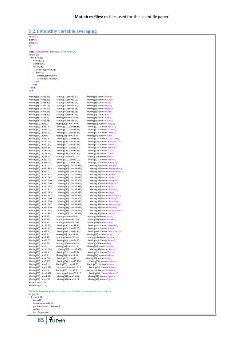
Matlab m-files: m-files used for the scientific paper

85

5.2.1 Monthly variable averaging m-file 40 clear all; close all; clc; load('Metingenmat','grond'); % result m-file 26 for j=0:10; for m=1:12; k=m+12*j; aantal(k)=1; for v=1:62; bi=isnan(grond(k,v)); if bi==0; doen(k,aantal(k))=v; aantal(k)=aantal(k)+1; end end end end Meting(1).Lat=13.33; Meting(1).Lon=33.37; Meting(1).Name='Sennar'; Meting(2).Lat=11.52; Meting(2).Lon=31.03; Meting(2).Name='Rashad'; Meting(3).Lat=13.10; Meting(3).Lon=30.14; Meting(3).Name='Obied'; Meting(4).Lat=12.03; Meting(4).Lon=24.53; Meting(4).Name='Nyala'; Meting(5).Lat=12.42; Meting(5).Lon=28.26; Meting(5).Name='Nahoud'; Meting(6).Lat=14.24; Meting(6).Lon=33.29; Meting(6).Name='Madini'; Meting(7).Lat=13.10; Meting(7).Lon=32.40; Meting(7).Name='Kosti'; Meting(8).Lat=15.6; Meting(8).Lon=32.549; Meting(8).Name='Khar'; Meting(9).Lat=15.28; Meting(9).Lon=36.24; Meting(9).Name='Kasala'; Meting(10).Lat=11; Meting(10).Lon=29.43; Meting(10).Name='Kadugli'; Meting(11).Lat=17.42; Meting(11).Lon=33.58; Meting(11).Name='Atbara'; Meting(12).Lat=14.02; Meting(12).Lon=35.24; Meting(12).Name='Gadarf'; Meting(13).Lat=13.37; Meting(13).Lon=25.20; Meting(13).Name='Fasher'; Meting(14).Lat=14; Meting(14).Lon=32.20; Meting(14).Name='Duem'; Meting(15).Lat=11.47; Meting(15).Lon=34.23; Meting(15).Name='Damazine'; Meting(16).Lat=11.20; Meting(16).Lon=27.49; Meting(16).Name='Babanusarai'; Meting(17).Lat=12.32; Meting(17).Lon=37.26; Meting(17).Name='Gondor'; Meting(18).Lat=23.58; Meting(18).Lon=32.47; Meting(18).Name='Asswan'; Meting(19).Lat=30.08; Meting(19).Lon=31.24; Meting(19).Name='Cairo'; Meting(20).Lat=25.40; Meting(20).Lon=32.42; Meting(20).Name='Luxor'; Meting(21).Lat=26.2; Meting(21).Lon=32.75; Meting(21).Name='Qena'; Meting(22).Lat=27.03; Meting(22).Lon=31.01; Meting(22).Name='Asyout'; Meting(23).Lat=28.05; Meting(23).Lon=30.44; Meting(23).Name='Elminya'; Meting(24).Lat=11.117; Meting(24).Lon=36.417; Meting(24).Name='Dangla'; Meting(25).Lat=11.883; Meting(25).Lon=38.033; Meting(25).Name='Debretabor'; Meting(26).Lat=12.117; Meting(26).Lon=37.867; Meting(26).Name='Addiszemen'; Meting(27).Lat=12.533; Meting(27).Lon=37.050; Meting(27).Name='Ayikel'; Meting(28).Lat=11.267; Meting(28).Lon=37.467; Meting(28).Name='Adet'; Meting(29).Lat=12.250; Meting(29).Lon=37.300; Meting(29).Name='Gorgora'; Meting(30).Lat=11.000; Meting(30).Lon=37.000; Meting(30).Name='Enjibara'; Meting(31).Lat=12.183; Meting(31).Lon=37.683; Meting(31).Name='Enfraz'; Meting(32).Lat=11.917; Meting(32).Lon=37.683; Meting(32).Name='Wereta'; Meting(33).Lat=11.683; Meting(33).Lon=37.317; Meting(33).Name='Zege'; Meting(34).Lat=12.367; Meting(34).Lon=37.550; Meting(34).Name='Maksegnit'; Meting(35).Lat=11.000; Meting(35).Lon=36.800; Meting(35).Name='Kidmaja'; Meting(36).Lat=11.550; Meting(36).Lon=37.380; Meting(36).Name='Kimbaba'; Meting(37).Lat=11.367; Meting(37).Lon=37.050; Meting(37).Name='Wetetabay'; Meting(38).Lat=10.950; Meting(38).Lon=37.070; Meting(38).Name='Gundil'; Meting(39).Lat=11.383; Meting(39).Lon=36.870; Meting(39).Name='AbaySheleko'; Meting(40).Lat=10.892; Meting(40).Lon=36.856; Meting(40).Name='Urana'; Meting(41).Lat=7.42; Meting(41).Lon=28.01; Meting(41).Name='Wau'; Meting(42).Lat=9.33; Meting(42).Lon=31.39; Meting(42).Name='Malakal'; Meting(43).Lat=4.52; Meting(43).Lon=31.36; Meting(43).Name='Juba'; Meting(44).Lat=10.33; Meting(44).Lon=38.13; Meting(44).Name='Yetemen'; Meting(45).Lat=10.43; Meting(45).Lon=36.57; Meting(45).Name='Shindi'; Meting(46).Lat=10.21; Meting(46).Lon=37.43; Meting(46).Name='Debremarcos'; Meting(47).Lat=7.2; Meting(47).Lon=35.42; Meting(47).Name='Teppi'; Meting(48).Lat=7.73; Meting(48).Lon=35.48; Meting(48).Name='Masha'; Meting(49).Lat=10.02; Meting(49).Lon=34.32; Meting(49).Name='Assosa'; Meting(50).Lat=9.35; Meting(50).Lon=34.53; Meting(50).Name='Begi'; Meting(51).Lat=11; Meting(51).Lon=37.13; Meting(51).Name='Sekela'; Meting(52).Lat=11.083; Meting(52).Lon=37.867; Meting(52).Name='Motta'; Meting(53).Lat=10.41; Meting(53).Lon=37.16; Meting(53).Name='Finote'; Meting(54).Lat=9.2; Meting(54).Lon=39.38; Meting(54).Name='Gebeya'; Meting(55).Lat=1.016; Meting(55).Lon=35; Meting(55).Name='Kitale'; Meting(56).Lat=0.405; Meting(56).Lon=35.224; Meting(56).Name='Eldoret'; Meting(57).Lat=-0.1; Meting(57).Lon=34.75; Meting(57).Name='Kisumu'; Meting(58).Lat=-1.333; Meting(58).Lon=31.817; Meting(58).Name='Bukoba'; Meting(59).Lat=-1.5; Meting(59).Lon=33.8; Meting(59).Name='Musoma'; Meting(60).Lat=-2.467; Meting(60).Lon=32.917; Meting(60).Name='Mwanza'; Meting(61).Lat=-4.88; Meting(61).Lon=29.63; Meting(61).Name='Kigoma'; Meting(62).Lat=-1.96; Meting(62).Lon=30.13; Meting(62).Name='Kigali'; y1=Meting(v).Lat; x1=Meting(v).Lon; %% find all possible grids and the amount of rainfall measurements inside that grid for j=0:10; for m=1:12; k=m+12*j; hoeveel=aantal(k)-1; punten=doen(k,1:hoeveel); welke=1; for p1=[punten];

Matlab m-files: m-files used for the scientific paper

86

y1=Meting(p1).Lat; x1=Meting(p1).Lon; for p2=[punten]; y2=Meting(p2).Lat; x2=Meting(p2).Lon; if p1==p2; Conclusie(welke,1,k)=1; Conclusie(welke,2,k)=y1; Conclusie(welke,3,k)=y1; Conclusie(welke,4,k)=x1; Conclusie(welke,5,k)=x1; Conclusie(welke,6,k)=1; Conclusie(welke,7,k)=0; Conclusie(welke,8,k)=0; Conclusie(welke,9,k)=Conclusie(welke,8,k)-Conclusie(welke,7,k); welke=welke+1; elseif p1<=p2; Conclusie(welke,1,k)=2; if y1>=y2; yas1=ceil(y1/0.25)*0.25; yas2=floor(y2/0.25)*0.25; afstandygroot=yas1-yas2; if x1<=x2; xas1=floor(x1/0.25)*0.25; xas2=xas1+afstandygroot; else xas2=ceil(x1/0.25)*0.25; xas1=xas2-afstandygroot; end Conclusie(welke,2,k)=yas1; Conclusie(welke,3,k)=yas2; Conclusie(welke,4,k)=xas1; Conclusie(welke,5,k)=xas2; aantalpunten=1; for p3=[punten]; if p3~=p1; y3=Meting(p3).Lat; x3=Meting(p3).Lon; if y3<=yas1 && y3>=yas2 && x3>=xas1 && x3<=xas2; aantalpunten=1+aantalpunten; end end end Conclusie(welke,6,k)=aantalpunten; Conclusie(welke,7,k)=yas1-yas2; Conclusie(welke,8,k)=xas2-xas1; Conclusie(welke,9,k)=Conclusie(welke,8,k)-Conclusie(welke,7,k); welke=welke+1; else yas2=floor(y1/0.25)*0.25; yas1=ceil(y2/0.25)*0.25; afstandygroot=yas1-yas2; if x1<=x2; xas1=floor(x1/0.25)*0.25; xas2=xas1+afstandygroot; else xas2=ceil(x1/0.25)*0.25; xas1=xas2-afstandygroot; end Conclusie(welke,2,k)=yas1; Conclusie(welke,3,k)=yas2; Conclusie(welke,4,k)=xas1; Conclusie(welke,5,k)=xas2; aantalpunten=1; for p3=[punten]; if p3~=p1; y3=Meting(p3).Lat; x3=Meting(p3).Lon; if y3<=yas1 && y3>=yas2 && x3>=xas1 && x3<=xas2; aantalpunten=1+aantalpunten; end end end Conclusie(welke,6,k)=aantalpunten; Conclusie(welke,7,k)=yas1-yas2; Conclusie(welke,8,k)=xas2-xas1; Conclusie(welke,9,k)=Conclusie(welke,8,k)-Conclusie(welke,7,k); welke=welke+1; end elseif p1>=p2; Conclusie(welke,1,k)=3; if x1>=x2; xas2=ceil(x1/0.25)*0.25; xas1=floor(x2/0.25)*0.25; afstandxgroot=xas2-xas1; if y1<=y2; yas2=floor(y1/0.25)*0.25; yas1=yas2+afstandxgroot; else yas1=ceil(y1/0.25)*0.25; yas2=yas1-afstandxgroot; end Conclusie(welke,2,k)=yas1; Conclusie(welke,3,k)=yas2; Conclusie(welke,4,k)=xas1; Conclusie(welke,5,k)=xas2; aantalpunten=1; for p3=[punten]; if p3~=p1;

Matlab m-files: m-files used for the scientific paper

87

y3=Meting(p3).Lat; x3=Meting(p3).Lon; if y3<=yas1 && y3>=yas2 && x3>=xas1 && x3<=xas2; aantalpunten=1+aantalpunten; end end end Conclusie(welke,6,k)=aantalpunten; Conclusie(welke,7,k)=yas1-yas2; Conclusie(welke,8,k)=xas2-xas1; Conclusie(welke,9,k)=Conclusie(welke,8,k)-Conclusie(welke,7,k); welke=welke+1; else xas1=floor(x1/0.25)*0.25; xas2=ceil(x2/0.25)*0.25; afstandxgroot=xas2-xas1; if y1<=y2; yas2=floor(y1/0.25)*0.25; yas1=yas2+afstandxgroot; else yas1=ceil(y1/0.25)*0.25; yas2=yas1-afstandxgroot; end Conclusie(welke,2,k)=yas1; Conclusie(welke,3,k)=yas2; Conclusie(welke,4,k)=xas1; Conclusie(welke,5,k)=xas2; aantalpunten=1; for p3=[punten]; if p3~=p1; y3=Meting(p3).Lat; x3=Meting(p3).Lon; if y3<=yas1 && y3>=yas2 && x3>=xas1 && x3<=xas2; aantalpunten=1+aantalpunten; end end end Conclusie(welke,6,k)=aantalpunten; Conclusie(welke,7,k)=yas1-yas2; Conclusie(welke,8,k)=xas2-xas1; Conclusie(welke,9,k)=Conclusie(welke,8,k)-Conclusie(welke,7,k); welke=welke+1; end end end end end end %% setting the requirements: 5 ground measurements and maximum of 5 degrees for k=1:132; welke=1; for i=1:size(Conclusie,1); if Conclusie(i,6,k)==5; Conclusie5(welke,:,k)=Conclusie(i,:,k); welke=welke+1; end end end for k=1:132; welke=1; for i=1:size(Conclusie5,1); if Conclusie5(i,7,k)<=5; Conclusie55(welke,:,k)=Conclusie5(i,:,k); welke=welke+1; end end end %% for k=1:132; hoeveel=aantal(k)-1; punten=doen(k,1:hoeveel); for punt=1:size(Conclusie55,1); welke=1; for p3=[punten]; if p3~=p1; y3=Meting(p3).Lat; x3=Meting(p3).Lon; if y3<=Conclusie55(punt,2,k) && y3>=Conclusie55(punt,3,k) && x3>=Conclusie55(punt,4,k) && x3<=Conclusie55(punt,5,k); gempunt(punt,welke,k)=p3; gempunt(punt,6,k)=Conclusie55(punt,2,k); gempunt(punt,7,k)=Conclusie55(punt,4,k); gempunt(punt,8,k)=Conclusie55(punt,7,k); welke=1+welke; end end end end end %% for k=1:size(gempunt,3);

Matlab m-files: m-files used for the scientific paper

88

A=gempunt(:,:,k); A1=gempunt(:,1:5,k); B=unique(A1,'rows'); for b=2:size(B,1); for a=1:size(A,1); if B(b,1)==A(a,1) && B(b,2)==A(a,2) && B(b,3)==A(a,3) && B(b,4)==A(a,4) && B(b,5)==A(a,5); C(b-1,1:5,k)=B(b,1:5); C(b-1,6:8,k)=A(a,6:8); end end end end %% for k=1:size(gempunt,3); j=1; for i=1:size(C,1); if C(i,5,k)~=0; D(j,:,k)=C(i,:,k); j=j+1; end end end %% for k=1:size(gempunt,3); for i=1:size(D,1); n=1; if D(i,2,k)>=0.1; for v=[D(i,1:5,k)]; P(n)=grond(k,v); n=1+n; end gemiddeld(i,1,k)=mean(P); gemiddeld(i,2:4,k)=D(i,6:8,k); P=0; else gemiddeld(i,1,k)=0; gemiddeld(i,2:4,k)=[0 0 0]; P=0; end end end %% finding the rainfall values of the products T(1,:)=[ones(1,80) 0 ones(1,51)]; % TAMSAT T(2,:)=[0 0 0 0 ones(1,127) 0]; % GSMaP T(3,:)=[zeros(1,36) ones(1,96)];% CMORPH T(4,:)=[0 0 ones(1,130)]; % PERSIANN T(5,:)=[zeros(1,12) ones(1,120)]; %RFE 2.0 h=waitbar(0,'Please wait...'); for k=1:size(gempunt,3); waitbar(k/132,h) openen=sprintf('GridBlock\\Triplekaarten\\TRMM%03d.mat',k); % result m-file 31 load(openen,'aveTRMM'); openen=sprintf('GridBlock\\Triplekaarten\\GPCP%03d.mat',k); % result m-file 31 load(openen,'aveGPCP'); openen=sprintf('GridBlock\\Triplekaarten\\GPCP1DD%03d.mat',k); % result m-file 31 load(openen,'aveGPCP1DD'); openen=sprintf('GridBlock\\Triplekaarten\\CRU%03d.mat',k); % result m-file 31 load(openen,'aveCRU'); openen=sprintf('GridBlock\\Triplekaarten\\ECMWF%03d.mat',k); % result m-file 31 load(openen,'aveECMWF'); openen=sprintf('GridBlock\\Triplekaarten\\ARC%03d.mat',k); % result m-file 31 load(openen,'aveARC'); openen=sprintf('GridBlock\\Triplekaarten\\CHIRPS%03d.mat',k); % result m-file 31 load(openen,'aveCHIRPS'); if T(5,k)==1; openen=sprintf('GridBlock\\Triplekaarten\\RFE%03d.mat',k); % result m-file 31 load(openen,'aveRFE'); end if T(4,k)==1; openen=sprintf('GridBlock\\Triplekaarten\\PERSIANN%03d.mat',k); % result m-file 31 load(openen,'avePERSIANN'); end if T(3,k)==1; openen=sprintf('GridBlock\\Triplekaarten\\CMORPH%03d.mat',k); % result m-file 31 load(openen,'aveCMORPH'); end if T(2,k)==1; openen=sprintf('GridBlock\\Triplekaarten\\GSMaP%03d.mat',k); % result m-file 31 load(openen,'aveGSMaP'); end if T(1,k)==1; openen=sprintf('GridBlock\\Triplekaarten\\TAMSAT%03d.mat',k); % result m-file 31 load(openen,'aveTAMSAT'); end openen=sprintf('GridBlock\\Triplekaarten\\TRIPLE%03d.mat',k); % result m-file 33 load(openen,'aveTRIPLE'); openen=sprintf('GridBlock\\Triplekaarten\\GPCC%03d.mat',k); % result m-file 31 load(openen,'aveGPCC'); for i=1:size(gemiddeld,1); if gemiddeld(i,2,k)~=0; yas=(40-gemiddeld(i,2,k))/0.25; xas=(gemiddeld(i,3,k)-20)/0.25;

Matlab m-files: m-files used for the scientific paper

89

aan=gemiddeld(i,4,k)/0.25-1; Vergelijk(i,1,k)=gemiddeld(i,1,k); TRMM=nanmean(nanmean(aveTRMM(yas:yas+aan,xas:xas+aan))); Vergelijk(i,2,k)=TRMM; GPCP=nanmean(nanmean(aveGPCP(yas:yas+aan,xas:xas+aan))); Vergelijk(i,3,k)=GPCP; GPCP1DD=nanmean(nanmean(aveGPCP1DD(yas:yas+aan,xas:xas+aan))); Vergelijk(i,4,k)=GPCP1DD; CRU=nanmean(nanmean(aveCRU(yas:yas+aan,xas:xas+aan))); Vergelijk(i,5,k)=CRU; ECMWF=nanmean(nanmean(aveECMWF(yas:yas+aan,xas:xas+aan))); Vergelijk(i,6,k)=ECMWF; ARC=nanmean(nanmean(aveARC(yas:yas+aan,xas:xas+aan))); Vergelijk(i,7,k)=ARC; CHIRPS=nanmean(nanmean(aveCHIRPS(yas:yas+aan,xas:xas+aan))); Vergelijk(i,8,k)=CHIRPS; if T(5,k)==1; RFE=nanmean(nanmean(aveRFE(yas:yas+aan,xas:xas+aan))); Vergelijk(i,9,k)=RFE; else Vergelijk(i,9,k)=NaN; end if T(4,k)==1; PERSIANN=nanmean(nanmean(avePERSIANN(yas:yas+aan,xas:xas+aan))); Vergelijk(i,10,k)=PERSIANN; else Vergelijk(i,10,k)=NaN; end if T(3,k)==1; CMORPH=nanmean(nanmean(aveCMORPH(yas:yas+aan,xas:xas+aan))); Vergelijk(i,11,k)=CMORPH; else Vergelijk(i,11,k)=NaN; end if T(2,k)==1; GSMaP=nanmean(nanmean(aveGSMaP(yas:yas+aan,xas:xas+aan))); Vergelijk(i,12,k)=GSMaP; else Vergelijk(i,12,k)=NaN; end if T(1,k)==1; TAMSAT=nanmean(nanmean(aveTAMSAT(yas:yas+aan,xas:xas+aan))); Vergelijk(i,13,k)=TAMSAT; else Vergelijk(i,13,k)=NaN; end TRIPLE=nanmean(nanmean(aveTRIPLE(yas:yas+aan,xas:xas+aan))); Vergelijk(i,15,k)=TRIPLE; GPCC=nanmean(nanmean(aveGPCC(yas:yas+aan,xas:xas+aan))); Vergelijk(i,14,k)=GPCC; else Vergelijk(i,:,k)=NaN; end end end %% j=1; for k=1:size(gempunt,3); for i=1:size(Vergelijk,1); if Vergelijk(i,1,k)~=0; Vergelijksamen(j,:)=Vergelijk(i,:,k); j=j+1; end end end Vergelijksamen=Vergelijksamen'; %% make scatter figure tekst3=['TRMM ';'GPCP ';'GPCP1DD ';'CRU ';'ECMWF ';'ARC ';'CHIRPS ';'RFE ';'PERSIANN';'CMORPH ';'GSMaP ';'TAMSAT ';'GPCC ';'TRIPLE ']; letters=[4 4 7 3 5 3 6 3 8 6 5 6 4 6]; for welkproduct=1:14; Vergelijktwee=[]; Vergelijktwee(1,:)=Vergelijksamen(1,:); Vergelijktwee(2,:)=Vergelijksamen((welkproduct+1),:); for i=1:length(Vergelijktwee); if Vergelijktwee(1,i)<=0; Vergelijktwee(1,i)=NaN; end end for i=1:length(Vergelijktwee); if Vergelijktwee(2,i)<=0; Vergelijktwee(2,i)=NaN; end end Vergelijktwee=Vergelijktwee(:,all(~isnan(Vergelijktwee))); for i=1:length(Vergelijktwee); if Vergelijktwee(1,i)<=0; Vergelijktwee(1,i)=NaN; end end Grond=Vergelijktwee(1,:); Product=Vergelijktwee(2,:); gemGrond=nanmean(Grond); gemProduct=nanmean(Product); sumGrond=sum(Grond); sumProduct=sum(Product); boven=sum((Grond-gemGrond).*(Product-gemProduct)); onder=sqrt(sum((Grond-gemGrond).^2))*sqrt(sum((Product-gemProduct).^2)); Corr(welkproduct)=boven/onder; Verschil=Product-Grond; Bias(welkproduct)=sum(Verschil)/length(Vergelijktwee);

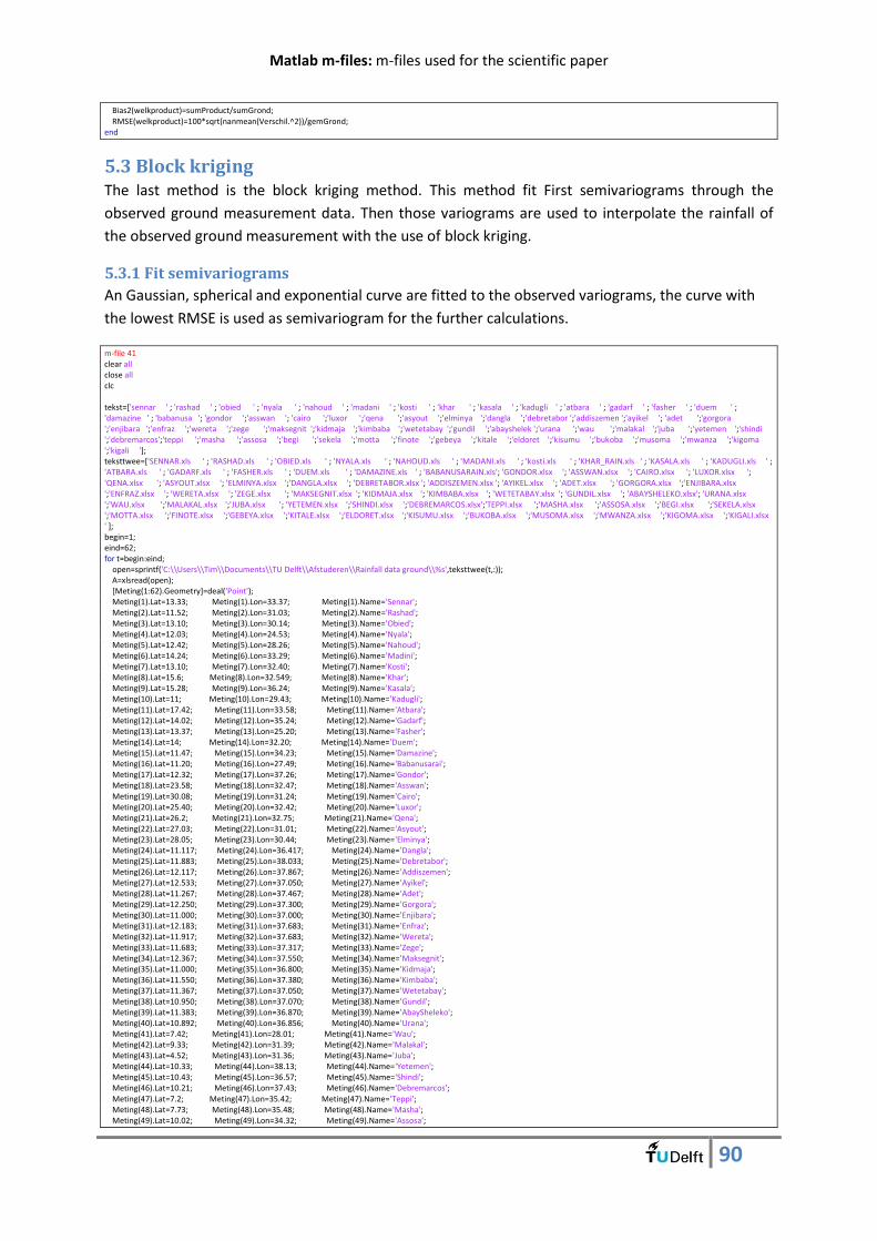
Matlab m-files: m-files used for the scientific paper

90

Bias2(welkproduct)=sumProduct/sumGrond; RMSE(welkproduct)=100*sqrt(nanmean(Verschil.^2))/gemGrond; end

5.3 Block kriging The last method is the block kriging method. This method fit First semivariograms through the

observed ground measurement data. Then those variograms are used to interpolate the rainfall of

the observed ground measurement with the use of block kriging.

5.3.1 Fit semivariograms

An Gaussian, spherical and exponential curve are fitted to the observed variograms, the curve with

the lowest RMSE is used as semivariogram for the further calculations.

m-file 41 clear all close all clc tekst=['sennar ' ; 'rashad ' ; 'obied ' ; 'nyala ' ; 'nahoud ' ; 'madani ' ; 'kosti ' ; 'khar ' ; 'kasala ' ; 'kadugli ' ; 'atbara ' ; 'gadarf ' ; 'fasher ' ; 'duem ' ; 'damazine ' ; 'babanusa '; 'gondor ';'asswan '; 'cairo ';'luxor ';'qena ';'asyout ';'elminya ';'dangla ';'debretabor ';'addiszemen ';'ayikel '; 'adet ';'gorgora ';'enjibara ';'enfraz ';'wereta ';'zege ';'maksegnit ';'kidmaja ';'kimbaba ';'wetetabay ';'gundil ';'abayshelek ';'urana ';'wau ';'malakal ';'juba ';'yetemen ';'shindi ';'debremarcos';'teppi ';'masha ';'assosa ';'begi ';'sekela ';'motta ';'finote ';'gebeya ';'kitale ';'eldoret ';'kisumu ';'bukoba ';'musoma ';'mwanza ';'kigoma ';'kigali ']; teksttwee=['SENNAR.xls ' ; 'RASHAD.xls ' ; 'OBIED.xls ' ; 'NYALA.xls ' ; 'NAHOUD.xls ' ; 'MADANI.xls ' ; 'kosti.xls ' ; 'KHAR_RAIN.xls ' ; 'KASALA.xls ' ; 'KADUGLI.xls ' ; 'ATBARA.xls ' ; 'GADARF.xls ' ; 'FASHER.xls ' ; 'DUEM.xls ' ; 'DAMAZINE.xls ' ; 'BABANUSARAIN.xls'; 'GONDOR.xlsx '; 'ASSWAN.xlsx '; 'CAIRO.xlsx '; 'LUXOR.xlsx '; 'QENA.xlsx '; 'ASYOUT.xlsx '; 'ELMINYA.xlsx ';'DANGLA.xlsx '; 'DEBRETABOR.xlsx '; 'ADDISZEMEN.xlsx '; 'AYIKEL.xlsx '; 'ADET.xlsx '; 'GORGORA.xlsx ';'ENJIBARA.xlsx ';'ENFRAZ.xlsx '; 'WERETA.xlsx '; 'ZEGE.xlsx '; 'MAKSEGNIT.xlsx '; 'KIDMAJA.xlsx '; 'KIMBABA.xlsx '; 'WETETABAY.xlsx '; 'GUNDIL.xlsx '; 'ABAYSHELEKO.xlsx'; 'URANA.xlsx ';'WAU.xlsx ';'MALAKAL.xlsx ';'JUBA.xlsx '; 'YETEMEN.xlsx ';'SHINDI.xlsx ';'DEBREMARCOS.xlsx';'TEPPI.xlsx ';'MASHA.xlsx ';'ASSOSA.xlsx ';'BEGI.xlsx ';'SEKELA.xlsx ';'MOTTA.xlsx ';'FINOTE.xlsx ';'GEBEYA.xlsx ';'KITALE.xlsx ';'ELDORET.xlsx ';'KISUMU.xlsx ';'BUKOBA.xlsx ';'MUSOMA.xlsx ';'MWANZA.xlsx ';'KIGOMA.xlsx ';'KIGALI.xlsx ' ]; begin=1; eind=62; for t=begin:eind; open=sprintf('C:\\Users\\Tim\\Documents\\TU Delft\\Afstuderen\\Rainfall data ground\\%s',teksttwee(t,:)); A=xlsread(open); [Meting(1:62).Geometry]=deal('Point'); Meting(1).Lat=13.33; Meting(1).Lon=33.37; Meting(1).Name='Sennar'; Meting(2).Lat=11.52; Meting(2).Lon=31.03; Meting(2).Name='Rashad'; Meting(3).Lat=13.10; Meting(3).Lon=30.14; Meting(3).Name='Obied'; Meting(4).Lat=12.03; Meting(4).Lon=24.53; Meting(4).Name='Nyala'; Meting(5).Lat=12.42; Meting(5).Lon=28.26; Meting(5).Name='Nahoud'; Meting(6).Lat=14.24; Meting(6).Lon=33.29; Meting(6).Name='Madini'; Meting(7).Lat=13.10; Meting(7).Lon=32.40; Meting(7).Name='Kosti'; Meting(8).Lat=15.6; Meting(8).Lon=32.549; Meting(8).Name='Khar'; Meting(9).Lat=15.28; Meting(9).Lon=36.24; Meting(9).Name='Kasala'; Meting(10).Lat=11; Meting(10).Lon=29.43; Meting(10).Name='Kadugli'; Meting(11).Lat=17.42; Meting(11).Lon=33.58; Meting(11).Name='Atbara'; Meting(12).Lat=14.02; Meting(12).Lon=35.24; Meting(12).Name='Gadarf'; Meting(13).Lat=13.37; Meting(13).Lon=25.20; Meting(13).Name='Fasher'; Meting(14).Lat=14; Meting(14).Lon=32.20; Meting(14).Name='Duem'; Meting(15).Lat=11.47; Meting(15).Lon=34.23; Meting(15).Name='Damazine'; Meting(16).Lat=11.20; Meting(16).Lon=27.49; Meting(16).Name='Babanusarai'; Meting(17).Lat=12.32; Meting(17).Lon=37.26; Meting(17).Name='Gondor'; Meting(18).Lat=23.58; Meting(18).Lon=32.47; Meting(18).Name='Asswan'; Meting(19).Lat=30.08; Meting(19).Lon=31.24; Meting(19).Name='Cairo'; Meting(20).Lat=25.40; Meting(20).Lon=32.42; Meting(20).Name='Luxor'; Meting(21).Lat=26.2; Meting(21).Lon=32.75; Meting(21).Name='Qena'; Meting(22).Lat=27.03; Meting(22).Lon=31.01; Meting(22).Name='Asyout'; Meting(23).Lat=28.05; Meting(23).Lon=30.44; Meting(23).Name='Elminya'; Meting(24).Lat=11.117; Meting(24).Lon=36.417; Meting(24).Name='Dangla'; Meting(25).Lat=11.883; Meting(25).Lon=38.033; Meting(25).Name='Debretabor'; Meting(26).Lat=12.117; Meting(26).Lon=37.867; Meting(26).Name='Addiszemen'; Meting(27).Lat=12.533; Meting(27).Lon=37.050; Meting(27).Name='Ayikel'; Meting(28).Lat=11.267; Meting(28).Lon=37.467; Meting(28).Name='Adet'; Meting(29).Lat=12.250; Meting(29).Lon=37.300; Meting(29).Name='Gorgora'; Meting(30).Lat=11.000; Meting(30).Lon=37.000; Meting(30).Name='Enjibara'; Meting(31).Lat=12.183; Meting(31).Lon=37.683; Meting(31).Name='Enfraz'; Meting(32).Lat=11.917; Meting(32).Lon=37.683; Meting(32).Name='Wereta'; Meting(33).Lat=11.683; Meting(33).Lon=37.317; Meting(33).Name='Zege'; Meting(34).Lat=12.367; Meting(34).Lon=37.550; Meting(34).Name='Maksegnit'; Meting(35).Lat=11.000; Meting(35).Lon=36.800; Meting(35).Name='Kidmaja'; Meting(36).Lat=11.550; Meting(36).Lon=37.380; Meting(36).Name='Kimbaba'; Meting(37).Lat=11.367; Meting(37).Lon=37.050; Meting(37).Name='Wetetabay'; Meting(38).Lat=10.950; Meting(38).Lon=37.070; Meting(38).Name='Gundil'; Meting(39).Lat=11.383; Meting(39).Lon=36.870; Meting(39).Name='AbaySheleko'; Meting(40).Lat=10.892; Meting(40).Lon=36.856; Meting(40).Name='Urana'; Meting(41).Lat=7.42; Meting(41).Lon=28.01; Meting(41).Name='Wau'; Meting(42).Lat=9.33; Meting(42).Lon=31.39; Meting(42).Name='Malakal'; Meting(43).Lat=4.52; Meting(43).Lon=31.36; Meting(43).Name='Juba'; Meting(44).Lat=10.33; Meting(44).Lon=38.13; Meting(44).Name='Yetemen'; Meting(45).Lat=10.43; Meting(45).Lon=36.57; Meting(45).Name='Shindi'; Meting(46).Lat=10.21; Meting(46).Lon=37.43; Meting(46).Name='Debremarcos'; Meting(47).Lat=7.2; Meting(47).Lon=35.42; Meting(47).Name='Teppi'; Meting(48).Lat=7.73; Meting(48).Lon=35.48; Meting(48).Name='Masha'; Meting(49).Lat=10.02; Meting(49).Lon=34.32; Meting(49).Name='Assosa';

Matlab m-files: m-files used for the scientific paper

91

Meting(50).Lat=9.35; Meting(50).Lon=34.53; Meting(50).Name='Begi'; Meting(51).Lat=11; Meting(51).Lon=37.13; Meting(51).Name='Sekela'; Meting(52).Lat=11.083; Meting(52).Lon=37.867; Meting(52).Name='Motta'; Meting(53).Lat=10.41; Meting(53).Lon=37.16; Meting(53).Name='Finote'; Meting(54).Lat=9.2; Meting(54).Lon=39.38; Meting(54).Name='Gebeya'; Meting(55).Lat=1.016; Meting(55).Lon=35; Meting(55).Name='Kitale'; Meting(56).Lat=0.405; Meting(56).Lon=35.224; Meting(56).Name='Eldoret'; Meting(57).Lat=-0.1; Meting(57).Lon=34.75; Meting(57).Name='Kisumu'; Meting(58).Lat=-1.333; Meting(58).Lon=31.817; Meting(58).Name='Bukoba'; Meting(59).Lat=-1.5; Meting(59).Lon=33.8; Meting(59).Name='Musoma'; Meting(60).Lat=-2.467; Meting(60).Lon=32.917; Meting(60).Name='Mwanza'; Meting(61).Lat=-4.88; Meting(61).Lon=29.63; Meting(61).Name='Kigoma'; Meting(62).Lat=-1.96; Meting(62).Lon=30.13; Meting(62).Name='Kigali'; y1=Meting(t).Lat; x1=Meting(t).Lon; B=A(1:11,2:13); B=B'; C=reshape(B,1,132); D(:,:,t)=C; end %% calculate the distance between 2 measurements load('O:\Metingenmat','grond'); % result m-file 26 D(:,:)=grond; for m=1:12; %months for x=1:62; % ground measurement point x0=Meting(x).Lon; y0=Meting(x).Lat; stappen=0.25; %step size of the intervals for y=1:62; if x==y; r(y)=0; else afy=abs(Meting(x).Lat-Meting(y).Lat); afx=abs(Meting(x).Lon-Meting(y).Lon); r(y)=sqrt(afx^2+afy^2); end end doen=zeros(30,10); for i=1:30; % calculate an inner and an outer circle with a maximum of 7.5 degrees welke=1; for y=1:62; r1=(i-1)*0.25; r2=i*0.25; if r(1,y)<=r2 && r(1,y)>=r1; % search for points within this range from the ground measurement point doen(i,welke)=y; welke=welke+1; end end end for i=1:30; r1=(i-1)*0.25; gebruiken=[]; gebruik=doen(i,:); welke=1; for j=1:10; if gebruik(1,j)>=0.1; gebruiken(1,welke)=gebruik(1,j); welke=welke+1; end end welke=1; TF=isempty(gebruiken); j=[0:10]; maanden=[m+[j]*12]; if TF~=1; for y=[gebruiken]; P(:,welke)=D(maanden,y); welke=welke+1; end E(:,1)=D(maanden,x); E(:,2)=nanmean(P,2); E=E'; E=E(:,all(~isnan(E))); TF=isempty(E); if TF~=1; Semivario=mean(E(1,:).^2)-2*mean(E(1,:).*E(2,:))+mean(E(2,:).^2); Vario(i,1)=0.5*Semivario; Afstand(i,1)=r1+stappen/2; else Vario(i,1)=NaN; Afstand(i,1)=NaN; end else Vario(i,1)=NaN; Afstand(i,1)=NaN; end E=[]; C=[]; end for q=1:length(Afstand); if Afstand(q,1)==0; Afstand(q,1)=NaN; end end R(1,:)=Afstand; R(2,:)=Vario;

Matlab m-files: m-files used for the scientific paper

92

R=R(:,all(~isnan(R))); Distance=R(1,:); TF=isempty(R); if TF~=1; if max(R(2,:))~=0; Variogram=R(2,:)/max(R(2,:)); Variogram2=R(2,:); else Variogram=R(2,:); Variogram2=R(2,:); end %% fit a Gaussian, spherical and exponential curve myfittype1=fittype('(c-c*exp((-x^2/b^2)))','dependent',{'y'},'independent',{'x'},'coefficients',{'b','c'}); myfittype2=fittype('(c*(((3/2)*(x/b)-0.5*(x^3/b^3))))','dependent',{'y'},'independent',{'x'},'coefficients',{'b','c'}); myfittype3=fittype('(c*(1-exp((-x/b))))','dependent',{'y'},'independent',{'x'},'coefficients',{'b','c'}); [myfit1,gof1]=fit(Distance',Variogram',myfittype1); [myfit2,gof2]=fit(Distance',Variogram',myfittype2); if m==5 && x==39 ||m==6 && x==40 ||m==10 && x==40;% some exceptions, was not possible to fit this curve myfit3.b=NaN; myfit3.c=NaN; gof3.rmse=NaN; else [myfit3,gof3]=fit(Distance',Variogram',myfittype3); end figure; fh1=@(x) (myfit1.c-myfit1.c*exp(-(x^2/(myfit1.b)^2))); fh2=@(x) (myfit2.c*((3/2)*(x/myfit2.b)-0.5*(x^3/myfit2.b^3))); fh3=@(x) (myfit3.c*(1-exp(-(x/(myfit3.b)^2)))); fplot(fh1,[0 20]); hold on; fplot(fh2,[0 20],'y'); fplot(fh3,[0 20],'c'); h=scatter(Distance,Variogram,'c'); A(x,1,m)=myfit1.b; A(x,2,m)=myfit1.c; A(x,3,m)=max(R(2,:)); A(x,4,m)=gof1.rmse; A(x,5,m)=myfit2.b; A(x,6,m)=myfit2.c; A(x,7,m)=max(R(2,:)); A(x,8,m)=gof2.rmse; A(x,9,m)=myfit3.b; A(x,10,m)=myfit3.c; A(x,11,m)=max(R(2,:)); A(x,12,m)=gof3.rmse; rmse(x,1:3)=A(x,[4 8 12],m); if min(rmse(x,:))==A(x,4,m); F(x,1,m)=A(x,4,m); F(x,2,m)=1; F(x,3,m)=A(x,1,m); F(x,4,m)=A(x,2,m); elseif min(rmse(x,:))==A(x,8,m); F(x,1,m)=A(x,8,m); F(x,2,m)=2; F(x,3,m)=A(x,5,m); F(x,4,m)=A(x,6,m); elseif min(rmse(x,:))==A(x,12,m); F(x,1,m)=A(x,12,m); F(x,2,m)=3; F(x,3,m)=A(x,9,m); F(x,4,m)=A(x,10,m); end F(x,5,m)=max(R(2,:)); else F(x,1:5,m)=NaN; end clearvars -except A F rmse m Meting D end end opslaan1=sprintf('O:\\Variancefitnieuw\\variancenieuwmaand.mat'); opslaan2=sprintf('O:\\Variancefitnieuw\\allevariancenieuwmaand.mat'); save(opslaan1,'F') save(opslaan2,'A')

5.3.2 Interpolate ground measurements using block kriging

Now this variogram is used in the block kriging method.

m-file 42 clear all close all clc for j=0:10; for m=1:12; l=m+12*j; size=0.25; %or grid 2.5 tekst=['sennar ' ; 'rashad ' ; 'obied ' ; 'nyala ' ; 'nahoud ' ; 'madani ' ; 'kosti ' ; 'khar ' ; 'kasala ' ; 'kadugli ' ; 'atbara ' ; 'gadarf ' ; 'fasher ' ; 'duem ' ; 'damazine ' ; 'babanusa '; 'gondor ';'asswan '; 'cairo ';'luxor ';'qena ';'asyout ';'elminya ';'dangla ';'debretabor ';'addiszemen ';'ayikel '; 'adet ';'gorgora ';'enjibara ';'enfraz ';'wereta ';'zege ';'maksegnit ';'kidmaja ';'kimbaba ';'wetetabay ';'gundil ';'abayshelek ';'urana ';'wau ';'malakal ';'juba ';'yetemen ';'shindi

Matlab m-files: m-files used for the scientific paper

93

';'debremarcos';'teppi ';'masha ';'assosa ';'begi ';'sekela ';'motta ';'finote ';'gebeya ';'kitale ';'eldoret ';'kisumu ';'bukoba ';'musoma ';'mwanza ';'kigoma ';'kigali ']; teksttwee=['SENNAR.xls ' ; 'RASHAD.xls ' ; 'OBIED.xls ' ; 'NYALA.xls ' ; 'NAHOUD.xls ' ; 'MADANI.xls ' ; 'kosti.xls ' ; 'KHAR_RAIN.xls ' ; 'KASALA.xls ' ; 'KADUGLI.xls ' ; 'ATBARA.xls ' ; 'GADARF.xls ' ; 'FASHER.xls ' ; 'DUEM.xls ' ; 'DAMAZINE.xls ' ; 'BABANUSARAIN.xls'; 'GONDOR.xlsx '; 'ASSWAN.xlsx '; 'CAIRO.xlsx '; 'LUXOR.xlsx '; 'QENA.xlsx '; 'ASYOUT.xlsx '; 'ELMINYA.xlsx ';'DANGLA.xlsx '; 'DEBRETABOR.xlsx '; 'ADDISZEMEN.xlsx '; 'AYIKEL.xlsx '; 'ADET.xlsx '; 'GORGORA.xlsx ';'ENJIBARA.xlsx ';'ENFRAZ.xlsx '; 'WERETA.xlsx '; 'ZEGE.xlsx '; 'MAKSEGNIT.xlsx '; 'KIDMAJA.xlsx '; 'KIMBABA.xlsx '; 'WETETABAY.xlsx '; 'GUNDIL.xlsx '; 'ABAYSHELEKO.xlsx'; 'URANA.xlsx ';'WAU.xlsx ';'MALAKAL.xlsx ';'JUBA.xlsx '; 'YETEMEN.xlsx ';'SHINDI.xlsx ';'DEBREMARCOS.xlsx';'TEPPI.xlsx ';'MASHA.xlsx ';'ASSOSA.xlsx ';'BEGI.xlsx ';'SEKELA.xlsx ';'MOTTA.xlsx ';'FINOTE.xlsx ';'GEBEYA.xlsx ';'KITALE.xlsx ';'ELDORET.xlsx ';'KISUMU.xlsx ';'BUKOBA.xlsx ';'MUSOMA.xlsx ';'MWANZA.xlsx ';'KIGOMA.xlsx ';'KIGALI.xlsx ' ]; sizeblock=0.05; %size block kringing sizeblockarea=2.5;% area which is taken into account for xas=1:30/size; % grid kolom for yas=1:50/size; % grid rij beginlon=20+(xas-1)*size; eindlon=20+(xas)*size; beginlat=40-(yas-1)*size; eindlat=40-(yas)*size; beginlonpunt=20+(xas-1)*size-sizeblockarea; eindlonpunt=20+(xas)*size+sizeblockarea; beginlatpunt=40-(yas-1)*size+sizeblockarea; eindlatpunt=40-(yas)*size-sizeblockarea; x1=linspace(beginlon+sizeblock/2,eindlon-sizeblock/2,size/sizeblock); y1=linspace(beginlat-sizeblock/2,eindlat+sizeblock/2,size/sizeblock); hoeveel=1; hoeveelpunt=1; for meting=1:62 % ground measurements Meting(1).Lat=13.33; Meting(1).Lon=33.37; Meting(1).Name='Sennar'; Meting(2).Lat=11.52; Meting(2).Lon=31.03; Meting(2).Name='Rashad'; Meting(3).Lat=13.10; Meting(3).Lon=30.14; Meting(3).Name='Obied'; Meting(4).Lat=12.03; Meting(4).Lon=24.53; Meting(4).Name='Nyala'; Meting(5).Lat=12.42; Meting(5).Lon=28.26; Meting(5).Name='Nahoud'; Meting(6).Lat=14.24; Meting(6).Lon=33.29; Meting(6).Name='Madini'; Meting(7).Lat=13.10; Meting(7).Lon=32.40; Meting(7).Name='Kosti'; Meting(8).Lat=15.6; Meting(8).Lon=32.549; Meting(8).Name='Khar'; Meting(9).Lat=15.28; Meting(9).Lon=36.24; Meting(9).Name='Kasala'; Meting(10).Lat=11; Meting(10).Lon=29.43; Meting(10).Name='Kadugli'; Meting(11).Lat=17.42; Meting(11).Lon=33.58; Meting(11).Name='Atbara'; Meting(12).Lat=14.02; Meting(12).Lon=35.24; Meting(12).Name='Gadarf'; Meting(13).Lat=13.37; Meting(13).Lon=25.20; Meting(13).Name='Fasher'; Meting(14).Lat=14; Meting(14).Lon=32.20; Meting(14).Name='Duem'; Meting(15).Lat=11.47; Meting(15).Lon=34.23; Meting(15).Name='Damazine'; Meting(16).Lat=11.20; Meting(16).Lon=27.49; Meting(16).Name='Babanusarai'; Meting(17).Lat=12.32; Meting(17).Lon=37.26; Meting(17).Name='Gondor'; Meting(18).Lat=23.58; Meting(18).Lon=32.47; Meting(18).Name='Asswan'; Meting(19).Lat=30.08; Meting(19).Lon=31.24; Meting(19).Name='Cairo'; Meting(20).Lat=25.40; Meting(20).Lon=32.42; Meting(20).Name='Luxor'; Meting(21).Lat=26.2; Meting(21).Lon=32.75; Meting(21).Name='Qena'; Meting(22).Lat=27.03; Meting(22).Lon=31.01; Meting(22).Name='Asyout'; Meting(23).Lat=28.05; Meting(23).Lon=30.44; Meting(23).Name='Elminya'; Meting(24).Lat=11.117; Meting(24).Lon=36.417; Meting(24).Name='Dangla'; Meting(25).Lat=11.883; Meting(25).Lon=38.033; Meting(25).Name='Debretabor'; Meting(26).Lat=12.117; Meting(26).Lon=37.867; Meting(26).Name='Addiszemen'; Meting(27).Lat=12.533; Meting(27).Lon=37.050; Meting(27).Name='Ayikel'; Meting(28).Lat=11.267; Meting(28).Lon=37.467; Meting(28).Name='Adet'; Meting(29).Lat=12.250; Meting(29).Lon=37.300; Meting(29).Name='Gorgora'; Meting(30).Lat=11.000; Meting(30).Lon=37.000; Meting(30).Name='Enjibara'; Meting(31).Lat=12.183; Meting(31).Lon=37.683; Meting(31).Name='Enfraz'; Meting(32).Lat=11.917; Meting(32).Lon=37.683; Meting(32).Name='Wereta'; Meting(33).Lat=11.683; Meting(33).Lon=37.317; Meting(33).Name='Zege'; Meting(34).Lat=12.367; Meting(34).Lon=37.550; Meting(34).Name='Maksegnit'; Meting(35).Lat=11.000; Meting(35).Lon=36.800; Meting(35).Name='Kidmaja'; Meting(36).Lat=11.550; Meting(36).Lon=37.380; Meting(36).Name='Kimbaba'; Meting(37).Lat=11.367; Meting(37).Lon=37.050; Meting(37).Name='Wetetabay'; Meting(38).Lat=10.950; Meting(38).Lon=37.070; Meting(38).Name='Gundil'; Meting(39).Lat=11.383; Meting(39).Lon=36.870; Meting(39).Name='AbaySheleko'; Meting(40).Lat=10.892; Meting(40).Lon=36.856; Meting(40).Name='Urana'; Meting(41).Lat=7.42; Meting(41).Lon=28.01; Meting(41).Name='Wau'; Meting(42).Lat=9.33; Meting(42).Lon=31.39; Meting(42).Name='Malakal'; Meting(43).Lat=4.52; Meting(43).Lon=31.36; Meting(43).Name='Juba'; Meting(44).Lat=10.33; Meting(44).Lon=38.13; Meting(44).Name='Yetemen'; Meting(45).Lat=10.43; Meting(45).Lon=36.57; Meting(45).Name='Shindi'; Meting(46).Lat=10.21; Meting(46).Lon=37.43; Meting(46).Name='Debremarcos'; Meting(47).Lat=7.2; Meting(47).Lon=35.42; Meting(47).Name='Teppi'; Meting(48).Lat=7.73; Meting(48).Lon=35.48; Meting(48).Name='Masha'; Meting(49).Lat=10.02; Meting(49).Lon=34.32; Meting(49).Name='Assosa'; Meting(50).Lat=9.35; Meting(50).Lon=34.53; Meting(50).Name='Begi'; Meting(51).Lat=11; Meting(51).Lon=37.13; Meting(51).Name='Sekela'; Meting(52).Lat=11.083; Meting(52).Lon=37.867; Meting(52).Name='Motta'; Meting(53).Lat=10.41; Meting(53).Lon=37.16; Meting(53).Name='Finote'; Meting(54).Lat=9.2; Meting(54).Lon=39.38; Meting(54).Name='Gebeya'; Meting(55).Lat=1.016; Meting(55).Lon=35; Meting(55).Name='Kitale'; Meting(56).Lat=0.405; Meting(56).Lon=35.224; Meting(56).Name='Eldoret'; Meting(57).Lat=-0.1; Meting(57).Lon=34.75; Meting(57).Name='Kisumu'; Meting(58).Lat=-1.333; Meting(58).Lon=31.817; Meting(58).Name='Bukoba'; Meting(59).Lat=-1.5; Meting(59).Lon=33.8; Meting(59).Name='Musoma'; Meting(60).Lat=-2.467; Meting(60).Lon=32.917; Meting(60).Name='Mwanza'; Meting(61).Lat=-4.88; Meting(61).Lon=29.63; Meting(61).Name='Kigoma'; Meting(62).Lat=-1.96; Meting(62).Lon=30.13; Meting(62).Name='Kigali'; if Meting(meting).Lat<=beginlat && Meting(meting).Lat>=eindlat && Meting(meting).Lon>=beginlon && Meting(meting).Lon<=eindlon IN(1:3,hoeveel)=[Meting(meting).Lat Meting(meting).Lon meting]; hoeveel=hoeveel+1; end if Meting(meting).Lat<=beginlatpunt && Meting(meting).Lat>=eindlatpunt && Meting(meting).Lon>=beginlonpunt && Meting(meting).Lon<=eindlonpunt

Matlab m-files: m-files used for the scientific paper

94

INpunt(1:3,hoeveelpunt)=[Meting(meting).Lat Meting(meting).Lon meting]; hoeveelpunt=hoeveelpunt+1; end end if hoeveel>1 A=zeros(length(x1)); Coord=[]; if hoeveel>1; i=1; for x=1:length(x1); for y=1:length(y1); Coord(i,1:2)=[x1(x) y1(y)]; i=i+1; end end i=i-1; if i>1; for x=1:i; for y=1:i; if x==y; A(x,y)=0; else x1=abs(Coord(x,1)-Coord(y,1)); y1=abs(Coord(x,2)-Coord(y,2)); A(x,y)=sqrt(x1^2+y1^2); end end end end else break end M=INpunt(3,:); for xl=1:length(M); open=sprintf('Rainfall data ground\\%s',teksttwee(M(xl),:)); data=xlsread(open); data=data(1:11,2:13); data=data'; data=reshape(data,1,132); Data(xl,1)=data(l); Data(xl,2)=INpunt(3,xl); Data(xl,3)=INpunt(1,xl); Data(xl,4)=INpunt(2,xl); Data1=Data'; Data2=Data1(:,all(~isnan(Data1))); end gebruikt=Data2(2,:); clear Data1 Data data M=IN(3,:); for xl=1:length(M); open=sprintf('Rainfall data ground\\%s',teksttwee(M(xl),:)); data=xlsread(open); data=data(1:11,2:13); data=data'; data=reshape(data,1,132); Data(xl,1)=data(l); Data(xl,2)=IN(3,xl); Data(xl,3)=IN(1,xl); Data(xl,4)=IN(2,xl); Data1=Data'; Data3=Data1(:,all(~isnan(Data1))); end gebruiktvar=Data3(2,:); Datadoor=Data1(1,:); i=1; if ((sum(isnan(Datadoor))))~=length(Datadoor); for p=[gebruikt]; lon(i)=Meting(p).Lon; lat(i)=Meting(p).Lat; i=i+1; end if length(lon)>=1; for x=1:length(lon); for y=1:length(lat); if x==y; D(x,y)=0; else x1=abs(lon(x)-lon(y)); y1=abs(lat(x)-lat(y)); D(x,y)=sqrt(x1^2+y1^2); end end end end x=1; y=1; for y=1:length(D); for x=1:length(A); x1=abs(Coord(x,1)-lon(y)); y1=abs(Coord(x,2)-lat(y)); B(x,y)=sqrt(x1^2+y1^2); end end C=B'; E=[A B;C D]; clear A B C D Coord Data Data1

Matlab m-files: m-files used for the scientific paper

95

o=1; for d=gebruikt; open=sprintf('Variancefitnieuw\\variancenieuwmaand.mat'); % result m-file 41 load(open,'F'); Coeff(1:5,o)=F(d,1:5,m); o=o+1; end o=o-1; for p=1:o; if Coeff(2,p)==1; hoogte(p)=Coeff(5,p)*Coeff(4,p); if (1-exp((-E.^2/Coeff(3,p)^2)))>=1; Ecov(:,:,p)=0; else Ecov(:,:,p)=1-1*(1-exp((-E.^2/Coeff(3,p)^2))); end elseif Coeff(2,Cop)==2; hoogte(p)=Coeff(5,p)*Coeff(4,p); if diff(1*(((3/2)*(E./Coeff(3,p))-0.5*(E.^3/Coeff(3,p)^3))))<0; Ecov(:,:,p)=0; else if (((3/2)*(E./Coeff(3,p))-0.5*(E.^3/Coeff(3,p)^3)))>=1; Ecov(:,:,p)=0; else Ecov(:,:,p)=1-1*(((3/2)*(E./Coeff(3,p))-0.5*(E.^3/Coeff(3,p)^3))); end end elseif Coeff(2,p)==3; hoogte(p)=Coeff(5,p)*Coeff(4,p); if diff(1*(1-exp((-E./Coeff(3,p)))))<0; Ecov(:,:,p)=0; else if 1*(1-exp((-E./Coeff(3,p))))>=1; Ecov(:,:,p)=0; else Ecov(:,:,p)=1-1*(1-exp((-E./Coeff(3,p)))); end end end end i=i-1; Ecovariance=mean(Ecov,3)*mean(hoogte(p)); D=ones(i+1); D(1:i,1:i)=Ecovariance(end-i+1:end,end-i+1:end); D(end,end)=0; for g=1:i; C(g)=mean(Ecovariance(length(Ecovariance)-i+g,1:length(Ecovariance)-i)); end C(i+1)=1; C=C'; W=D\C; regen=Data2(1,:)'; Z=sum(W(1:length(W)-1).*regen); Ca=mean(Ecovariance(1:length(Ecovariance)-i,1:length(Ecovariance)-i)); Caa=mean(Ca); deel2=sum(W(1:i).*C(1:i))+W(i+1); sigma=sqrt(abs(Caa-(deel2))); ResultZ(xas,yas,l)=Z; Resultsigma(xas,yas,l)=sigma; else ResultZ(xas,yas,l)=NaN; Resultsigma(xas,yas,l)=NaN; end else ResultZ(xas,yas,l)=NaN; Resultsigma(xas,yas,l)=NaN; end clearvars -except Ecovariance ResultZ Resultsigma j m xas yas size tekst teksttwee sizeblock l sizeblockarea end end end end save('Meetpuntennieuw\\sigma025meet25grid.mat','Resultsigma'); save('Meetpuntennieuw\\Z025meet25grid.mat','ResultZ');

5.3.3 Comparison between Block kriging and products

This m-file makes for every pixel a .mat file which consists of all the values of all the products and the

ground measurements interpolated with block kriging. The m-file below is for the 0.25 degrees

resolution, almost the same format is used for the 2.5 degree resolution

m-file 43 clear all; close all; clc; load('GridBlock\Pixels025.mat','P'); % selection of which pixel must be calculated % result m-file 34 method=sprintf('nearest'); for Kolom=1:120; % 12 for 2.5 degrees resolution for Rij=1:200; % 20 for 2.5 degrees resolution

Matlab m-files: m-files used for the scientific paper

96

grid=0.25; B=zeros(50/grid,30/grid); for y=0:10; for m=1:12; k=y*12+m; if P(Kolom,Rij,k)==1; open=sprintf('GridBlock\\Meetpunten025\\Z025meet25grid.mat'); % result m-file 43 load(open,'ResultZ'); if isnan(ResultZ(Kolom,Rij,k)); P(k,1)=NaN; else E=ResultZ(Kolom,Rij,k); P(k,1)=E; T(1,:)=[ones(1,80) 0 ones(1,51)]; % TAMSAT T(2,:)=[0 0 0 0 ones(1,127) 0]; % GSMaP T(3,:)=[zeros(1,36) ones(1,96)];% CMORPH T(4,:)=[0 0 ones(1,130)]; % PERSIANN T(5,:)=[zeros(1,12) ones(1,120)]; %RFE 2.0 end %% TRMM k=y*12+m; openen=sprintf('GridBlock\\Kaarten025\\TRMM%03d.mat',k); % result m-file 31 load(openen,'aveTRMM'); D=aveTRMM(Rij,Kolom); P(k,2)=D; D=0; %% GPCP k=y*12+m; openen=sprintf('GridBlock\\Kaarten025\\GPCP%03d.mat',k); % result m-file 31 load(openen,'aveGPCP'); D=aveGPCP(Rij,Kolom); P(k,3)=D; %% GPCP1DD k=y*12+m; openen=sprintf('GridBlock\\Kaarten025\\GPCP1DD%03d.mat',k); % result m-file 31 load(openen,'aveGPCP1DD'); D=aveGPCP1DD(Rij,Kolom); P(k,4)=D; %% CRU k=y*12+m; openen=sprintf('GridBlock\\Kaarten025\\CRU%03d.mat',k); % result m-file 31 load(openen,'aveCRU'); D=aveCRU(Rij,Kolom); P(k,5)=D; %% ECMWF k=y*12+m; openen=sprintf('GridBlock\\Kaarten025\\ECMWF%03d.mat',k); % result m-file 31 load(openen,'aveECMWF'); D=aveECMWF(Rij,Kolom); P(k,6)=D; %% ARC 2.0 k=y*12+m; openen=sprintf('GridBlock\\Kaarten025\\ARC%03d.mat',k); % result m-file 31 load(openen,'aveARC'); D=aveARC(Rij,Kolom); P(k,7)=D; %% CHIRPS 8 k=y*12+m; openen=sprintf('GridBlock\\Kaarten025\\CHIRPS%03d.mat',k); % result m-file 31 load(openen,'aveCHIRPS'); D=aveCHIRPS(Rij,Kolom); P(k,8)=D; %% RFE 9 t=y*12+m; k=y*12+m; if T(5,t)==1; k=y*12+m; openen=sprintf('GridBlock\\Kaarten025\\RFE%03d.mat',k); % result m-file 31 load(openen,'aveRFE'); D=aveRFE(Rij,Kolom); P(k,9)=D; else P(k,9)=NaN; end %% PERSIANN 10 t=y*12+m; k=y*12+m; if T(4,t)==1; k=y*12+m; openen=sprintf('GridBlock\\Kaarten025\\PERSIANN%03d.mat',k); % result m-file 31 load(openen,'avePERSIANN'); D=avePERSIANN(Rij,Kolom); k=y*12+m; P(k,10)=D; else P(k,10)=NaN; end

Matlab m-files: m-files used for the scientific paper

97

%% CMORPH 11 t=y*12+m; k=y*12+m; if T(3,t)==1; k=y*12+m; openen=sprintf('GridBlock\\Kaarten025\\CMORPH%03d.mat',k); % result m-file 31 load(openen,'aveCMORPH'); D=aveCMORPH(Rij,Kolom); k=y*12+m; P(k,11)=D; else P(k,11)=NaN; end %% GSMaP 12 t=y*12+m; k=y*12+m; if T(2,t)==1; k=y*12+m; openen=sprintf('GridBlock\\Kaarten025\\GSMaP%03d.mat',k); % result m-file 31 load(openen,'aveGSMaP'); D=aveGSMaP(Rij,Kolom); P(k,12)=D; else P(k,12)=NaN; end %% TAMSAT t=y*12+m; k=y*12+m; if T(1,t)==1; k=y*12+m; openen=sprintf('GridBlock\\Kaarten025\\TAMSAT%03d.mat',k); % result m-file 31 load(openen,'aveTAMSAT'); D=aveTAMSAT(Rij,Kolom); k=y*12+m; P(k,13)=D; else P(k,13)=NaN; end %% GPCC k=y*12+m; openen=sprintf('GridBlock\\Kaarten025\\GPCC%03d.mat',k); % result m-file 31 load(openen,'aveGPCC'); D=aveGPCC(Rij,Kolom); P(k,14)=D; %% Triple t=y*12+m; k=y*12+m; openen=sprintf('GridBlock\\Kaarten025\\TRIPLE%03d.mat',k); % result m-file 33 load(openen,'aveTRIPLE'); D=aveTRIPLE(Rij,Kolom); k=y*12+m; P(k,15)=D; else P(k,1:13)=NaN; end end end opslaan=sprintf('GridBlock\\025meet\\x%02dy%02d.mat',Kolom,Rij); save(opslaan,'P'); end end

5.3.4 Validation using the block kriging method

The last m-file calculates the correlation, bias, and the RMSE of the products. This is done for the

monthly and yearly rainfall values. Different areas can be calculated by using different pixel selection

maps.

Yearly:

m-file 44 clear all; close all; clc; tekst3=['TRMM ';'GPCP ';'GPCP1DD ';'CRU ';'ECMWF ';'ARC ';'CHIRPS ';'RFE ';'PERSIANN';'CMORPH ';'GSMaP ';'TAMSAT ']; letters=[4 4 7 3 5 3 6 3 8 6 5 6]; grid=2.5; getal=25; load('GridBlock\Pixels25bluenile.mat','PX'); %pixel selection:P for whole basin % result m-file 35 K=PX;%P for whole basin PX=0;%P for whole basin for welkproduct=1:14; Vergelijk=[]; Vergelijktwee=[]; aantal=1; for x=1:30/grid; for y=1:50/grid;

Matlab m-files: m-files used for the scientific paper

98

for j=0:10; for m=1:12;%1:132; l=m+12*j; if K(x,y,l)==1; openen=sprintf('GridBlock\\%dmeet\\x%02dy%02d.mat',getal,x,y); % result m-file 43 load(openen,'P'); P1(m)=P(l,1); P2(m)=P(l,welkproduct+1); Vergelijk(1,aantal)=mean(P1)*12; Vergelijk(2,aantal)=mean(P2)*12; Vergelijk(3,aantal)=x; Vergelijk(4,aantal)=y; aantal=aantal+1; end end end end end for i=1:length(Vergelijk); if Vergelijk(1,i)<=0; Vergelijk(1,i)=NaN; end end for i=1:length(Vergelijk); if Vergelijk(2,i)<=0; Vergelijk(2,i)=NaN; end end Vergelijk=Vergelijk(:,all(~isnan(Vergelijk))); for i=1:length(Vergelijk); if Vergelijk(1,i)<=0; Vergelijk(1,i)=NaN; end end Grond=Vergelijk(1,:); Product=Vergelijk(2,:); Vergelijktwee(1,:)=Vergelijk(1,:); Vergelijktwee(2,:)=Vergelijk(2,:); gemGrond=nanmean(Grond); gemProduct=nanmean(Product); sumGrond=sum(Grond); sumProduct=sum(Product); boven=sum((Grond-gemGrond).*(Product-gemProduct)); onder=sqrt(sum((Grond-gemGrond).^2))*sqrt(sum((Product-gemProduct).^2)); Corr2(welkproduct)=(length(Grond)*sum(Grond.*Product)-sumGrond*sumProduct)/(sqrt(length(Grond)*sum(Grond.^2)-sum(Grond)^2)*sqrt(length(Grond)*sum(Product.^2)-sum(Product)^2)); Corr(welkproduct)=boven/onder; Verschil=Product-Grond; Bias(welkproduct)=sum(Verschil)/length(Vergelijktwee); Bias2(welkproduct)=sumProduct/sumGrond; RMSE(welkproduct)=100*sqrt(nanmean(Verschil.^2))/gemGrond; end %% for scatter plot figure(1); plot(1:10,1:10); hold on; plot(1:6,1:6); h=legend('test ','test2 ','Location','NorthWest') handle = get(h); close(figure(1)); Grond=Vergelijk(1,:); Product=Vergelijk(2,:); % fill in product number p=figure(2) p=figure('units','normalized','outerposition',[0 0 1 1]); gemGrond=nanmean(Grond); gemProduct=nanmean(Product); boven=sum((Grond-gemGrond).*(Product-gemProduct)); onder=sqrt(sum((Grond-gemGrond).^2))*sqrt(sum((Product-gemProduct).^2)); Corr=boven/onder; Verschil=Product-Grond; Bias=sum(Verschil)/length(Vergelijk); RMSE=sqrt(nanmean(Verschil.^2)); str={sprintf('Corr = %0.03f',Corr),sprintf('RMSE = %0.2f',RMSE),sprintf('Bias=%0.2f',Bias)}; fw=@(x) x; fplot(fw,[0 3000],'c--'); hold on plot(Grond,Product,'.'); xlabel('Ground Measurement'); ylabel('Product Estimation'); annotation('textbox',handle.UserData.LegendPosition,'String',str,'EdgeColor','none'); titel=sprintf('%s Yearly Nile Basin %0.2f degrees',tekst3(welkproduct,1:letters(welkproduct)),grid); title(titel);

Monthly:

m-file 45 clear all; close all; clc;

Matlab m-files: m-files used for the scientific paper

99

tekst3=['TRMM ';'GPCP ';'GPCP1DD ';'CRU ';'ECMWF ';'ARC ';'CHIRPS ';'RFE ';'PERSIANN';'CMORPH ';'GSMaP ';'TAMSAT ';'GPCC ';'TRIPLE ']; letters=[4 4 7 3 5 3 6 3 8 6 5 6 4 6]; grid=0.25; % if 2.5degrees than grid =2.5 getal=25; load('GridBlock\Pixels025.mat','P'); %pixel selection: PX for subbasin % result m-file 34 K=P;%PX for subbasin P=0;%PX for subbasin for welkproduct=1:14; aantal=1; Vergelijk=[]; Vergelijktwee=[]; for x=1:30/grid; for y=1:50/grid; for l=1:132; if K(x,y,l)==1; openen=sprintf('GridBlock\\0%dmeet\\x%02dy%02d.mat',getal,x,y); % result m-file 43 load(openen,'P'); Vergelijk(1,aantal)=P(l,1); Vergelijk(2,aantal)=P(l,welkproduct+1); aantal=aantal+1; end end end end for i=1:length(Vergelijk); if Vergelijk(1,i)<=0; Vergelijk(1,i)=NaN; end end for i=1:length(Vergelijk); if Vergelijk(2,i)<=0; Vergelijk(2,i)=NaN; end end Vergelijk=Vergelijk(:,all(~isnan(Vergelijk))); for i=1:length(Vergelijk); if Vergelijk(1,i)<=0; Vergelijk(1,i)=NaN; end end Grond=Vergelijk(1,:); Product=Vergelijk(2,:); Vergelijktwee(1,:)=Vergelijk(1,:); Vergelijktwee(2,:)=Vergelijk(2,:); gemGrond=nanmean(Grond); gemProduct=nanmean(Product); sumGrond=sum(Grond); sumProduct=sum(Product); boven=sum((Grond-gemGrond).*(Product-gemProduct)); onder=sqrt(sum((Grond-gemGrond).^2))*sqrt(sum((Product-gemProduct).^2)); Corr(welkproduct)=boven/onder; Verschil=Product-Grond; Bias(welkproduct)=sum(Verschil)/length(Vergelijktwee); Bias2(welkproduct)=sumProduct/sumGrond; RMSE(welkproduct)=100*sqrt(nanmean(Verschil.^2))/gemGrond; end %% for scatter plot welkeproduct=6; %fill in the product 1=TRMM 2=GPCP 3=GPCP1DD 4=CRU 5=ECMWF 6=ARC 7=CHIRPS 8=RFE 9=PERSIANN 10=CMORPH 11=GSMaP 12=TAMSAT 13=GPCC 14=TRIPLE

Vergelijktwee(1,:)=Vergelijk(1,:); Vergelijktwee(2,:)=Vergelijk(welkeproduct+1,:); figure(1); plot(1:10,1:10); hold on; plot(1:6,1:6); h=legend('test ','test2 ','Location','NorthWest') handle = get(h); close(figure(1)); Grond=Vergelijktwee(1,:); Product=Vergelijktwee(2,:); p=figure(2) p=figure('units','normalized','outerposition',[0 0 1 1]); gemGrond=nanmean(Grond); gemProduct=nanmean(Product); boven=sum((Grond-gemGrond).*(Product-gemProduct)); onder=sqrt(sum((Grond-gemGrond).^2))*sqrt(sum((Product-gemProduct).^2)); Corr=boven/onder; Verschil=Product-Grond; Bias=sum(Verschil)/length(Vergelijk); RMSE=sqrt(nanmean(Verschil.^2)); str={sprintf('Corr = %0.03f',Corr),sprintf('RMSE = %0.2f',RMSE),sprintf('Bias=%0.2f',Bias)}; fw=@(x) x; fplot(fw,[0 max(Product)],'c--'); hold on plot(Grond,Product,'.'); xlabel('Ground Measurement'); ylabel('Product Estimation'); annotation('textbox',handle.UserData.LegendPosition,'String',str,'EdgeColor','none'); titel=sprintf('%s Nile Basin %0.2f degrees',tekst3(welkproduct,1:letters(welkproduct)),grid); title(titel);

Matlab m-files: m-files used for the scientific paper

100

6. Pictures in paper

6.1 Figure 1: Made with QGIS. (A) is the DEM map clipped for the Nile Basin. The river is found by using r.watershed en the lake is made by using r.lake. The editing is done in the editor of QGIS. (B) averaging the yearly rainfall from the TRMM product which was calculated in m-file 24. This averaging is done in QGIS. Also the editing is done in QGIS. (C) plotting the subbasins shapefiles in QGIS and edited in the editor of QGIS. The picture is made in adobe illustrator.

6.2 Figure 2: This picture is made with QGIS, with the shapefiles for the point measurements made in Matlab, see m-file 27 by saving the Meting parameter as a shapefile. The editing part is done in adobe illustrator.

6.3 Figure 3: The maps are made in matlab with m-file 31. The editing is done in QGIS and adobe illustrator.

6.4 Figure 4: Is made with the following m-file: m-file 46 clear all; close all; clc; %% load('Balkplaatje.mat'); % made in excel with the use of the results of m-file 20 Jaar=zeros(14,11); for y=0:10; for m=1:14; Jaar(m,y+1)=sum(T(m,y*12+1:y*12+12)); end end for m=1:14; gem(m)=nanmean(Jaar(m,4:10)); max(m)=nanmean(Jaar(m,8)); min(m)=nanmean(Jaar(m,5)); end figure(1); %% fh=bar(gem,0.9,'k'); set(gca,'Box','off'); set(gcf,'units','centimeters'); set(gcf,'papersize',[30,50]); set(gcf,'paperposition',[0,0,38,20]); set(gca,'XTickLabel',{'TRMM','GPCP','GPCP1DD','CRU','ECMWF','ARC 2.0','CHIRPS','RFE 2.0','PERSIANN','CMORPH','GSMaP','TAMSAT','GPCC','TRIPLE'},'FontSize',7); xticklabel_rotate([1 2 3 4 5 6 7 8 9 10 11 12 13 14],90,{'TRMM','GPCP','GPCP1DD','CRU','ECMWF','ARC 2.0','CHIRPS','RFE 2.0','PERSIANN','CMORPH','GSMaP','TAMSAT','GPCC','TRIPLE'},'FontSize',9); titel=sprintf('Mean Rainfall of the products 2003-2009 over the Nile Basin'); title(titel,'FontSize',14); ylabel('Precipitation in millimeters','FontSize',9); %set(fh,'color','white'); saveas(fh,'meanrainfallnilebasin','epsc'); %% fh=bar(max,0.9,'k'); set(gca,'Box','off'); set(gcf,'units','centimeters'); set(gcf,'papersize',[30,50]); set(gcf,'paperposition',[0,0,38,20]); set(gca,'XTickLabel',{'TRMM','GPCP','GPCP1DD','CRU','ECMWF','ARC 2.0','CHIRPS','RFE 2.0','PERSIANN','CMORPH','GSMaP','TAMSAT','GPCC','TRIPLE'},'FontSize',7); xticklabel_rotate([1 2 3 4 5 6 7 8 9 10 11 12 13 14],90,{'TRMM','GPCP','GPCP1DD','CRU','ECMWF','ARC 2.0','CHIRPS','RFE 2.0','PERSIANN','CMORPH','GSMaP','TAMSAT','GPCC','TRIPLE'},'FontSize',9); titel=sprintf('Rainfall of the products over the Nile Basin during wet year 2007'); title(titel,'FontSize',14); ylabel('Precipitation in millimeters','FontSize',9); saveas(fh,'wetrainfallnilebasin','epsc'); %% x=[1,2,3,4,5,6,7,8,9,10,11,12,13,14]; fh=bar(x,min,0.9,'k'); set(gca,'Box','off'); set(gcf,'units','centimeters'); set(gcf,'papersize',[30,50]); set(gcf,'paperposition',[0,0,38,20]); set(gca,'XTickLabel',{'TRMM','GPCP','GPCP1DD','CRU','ECMWF','ARC 2.0','CHIRPS','RFE 2.0','PERSIANN','CMORPH','GSMaP','TAMSAT','GPCC','TRIPLE'},'FontSize',7); xticklabel_rotate([1 2 3 4 5 6 7 8 9 10 11 12 13 14],90,{'TRMM','GPCP','GPCP1DD','CRU','ECMWF','ARC 2.0','CHIRPS','RFE 2.0','PERSIANN','CMORPH','GSMaP','TAMSAT','GPCC','TRIPLE'},'FontSize',9); titel=sprintf('Rainfall of the products over the Nile Basin during dry year 2004');

Matlab m-files: m-files used for the scientific paper

101

title(titel,'FontSize',14); ylabel('Precipitation in millimeters','FontSize',9); set(fh,'color','white'); saveas(fh,'dryrainfallnilebasin','epsc');

Some editing is done in adobe illustrator.

6.5 Figure 5: The boxplots are made with the following m-file:

m-file 47

clear all;

close all;

clc;

%%

A=xlsread('nilebasinrainfall20032010.xlsx'); % yearly results for the nile calculated with m-file 20

Jaar=zeros(14,11);

for maand=1:12;

for m=1:14;

y=[0:7];

maandwelke=[36+y*12+maand];

maandmean(m,maand)=nanmean(A(m,maandwelke));

end

end

for m=1:14;

for y=1:8;

for maand=1:12;

i=24+maand+y*12;

maandannomalies(m,i-36)=100*(A(m,i)/maandmean(m,maand));

end

end

end

for m=1:14;

for y=1:8;

for maand=1:12;

i=24+maand+y*12;

maandannomalies2(m,i-36)=(A(m,i)-maandmean(m,maand));

end

end

end

for maand=6:9

h=figure(maand);

y=[0:7];

box=maandannomalies(:,[y*12+maand]);

box=box';

for m=1:14;

y=[0:7];

h=plot(m,box(:,m),'b+');

hold on;

minima=min(box(:,m));

maxima=max(box(:,m));

h=plot(m,minima,'ko','linewidth',3);

h=plot(m,maxima,'ko','linewidth',3);

hold on;

labels={'TRMM' 'GPCP' 'GPCP1DD' 'CRU' 'ECMWF' 'ARC' 'CHIRPS' 'RFE' 'PERSIANN' 'CMORPH' 'GSMaP' 'TAMSAT' 'GPCC'

'TRIPLE'};

set(gca, 'XTick',1:14,'XTickLabel',labels);

end

end

for maand=6:9

h=figure(maand);

y=[0:7];

box=maandannomalies2(:,[y*12+maand]);

box=box';

for m=1:14;

y=[0:7];

h=plot(m,box(:,m),'b+');

hold on;

minima=min(box(:,m));

maxima=max(box(:,m));

h=plot(m,minima,'ko','linewidth',3);

h=plot(m,maxima,'ko','linewidth',3);

hold on;

labels={'TRMM' 'GPCP' 'GPCP1DD' 'CRU' 'ECMWF' 'ARC' 'CHIRPS' 'RFE' 'PERSIANN' 'CMORPH' 'GSMaP' 'TAMSAT' 'GPCC'

'TRIPLE'};

set(gca, 'XTick',1:14,'XTickLabel',labels);

end

end

for maand=6:9

h=figure(maand);

y=[0:7];

box=maandannomalies(:,[y*12+maand]);

box=box';

boxplot(box(:,:),'Labels',{'TRMM','GPCP','GPCP1DD','CRU','ECMWF','ARC','CHIRPS','RFE','PERSIANN','CMORPH','GSMaP','TAMSAT','G

PCC','TRIPLE'});

end

Matlab m-files: m-files used for the scientific paper

102

Editing is done in adobe illustrator

6.6 Figure 6: Is made with the following m-file:

m-file 48 clear all;

close all;

clc;

%%

for t=1:16;%which basin

method=sprintf('nearest'); %bicubic nearest or bilinear

basin=['Nilebasin.shp ';'albertnilebahraljabal.shp';'bahrelghazal.shp ';'baroakobosobat.shp

';'bluenile.shp ';'kagera.shp ';'lakevictoria.shp ';'lowerwhitenile.shp

';'mainnile1.shp ';'mainnile2.shp ';'mainnile3.shp ';'mainnile4.shp

';'semlikilalbert.shp ';'sudd.shp ';'tekezzeatbara.shp ';'victorianile.shp '];

U=[13 25 16 18 12 10 16 18 13 13 13 13 18 8 17 16];

gebied=sprintf('C:\\Users\\Tim\\Documents\\TU Delft\\Afstuderen\\Data\\Layers\\sub\\%s',basin(t,1:U(t)));

% Nilebasin, albertnilebahraljabal, bahrelghazal, baroakobosobat,

% bluenile,kagera, lakevictoria, lowerwhitenile, mainnile1, mainnile2,

% mainnile3, mainnile4, semlikilalbert, sudd, tekezzeatbara or

% victorianile

%% maken masker gebied

Nilebasin = shaperead(gebied,'UseGeoCoords',true);

inLat=Nilebasin.Lat;

inLon=Nilebasin.Lon;

gridDensity=10;

[inGrid,InRefVec]=vec2mtx(inLat,inLon,gridDensity);

Masker=zeros(500,300);

Mask = imfill(inGrid,'holes');

a1=floor(Nilebasin.BoundingBox(1,2)*10)/10-0.2;

a2=floor(Nilebasin.BoundingBox(2,2)*10)/10+0.2;

a3=floor(Nilebasin.BoundingBox(1,1)*10)/10-0.2;

a4=floor(Nilebasin.BoundingBox(2,1)*10)/10+0.2;

R1 = georasterref('RasterSize', size(Mask),'Latlim', [a1 a2], 'Lonlim', [a3 a4],'ColumnsStartFrom','south');

%geoshow(Mask,R1,'DisplayType', 'Texturemap');

%geoshow(Nilebasin.Lat,Nilebasin.Lon,'DisplayType','line','Color','k')

grote=size(Mask);

b1=grote(1)-1;

b2=grote(2)-1;

c1=(a1+10)*10+1;

c2=(a3-20)*10+1;

Masker(c1:c1+b1,c2:c2+b2)=Masker(c1:c1+b1,c2:c2+b2)+Mask;

R2 = georasterref('RasterSize', size(Masker),'Latlim', [-10 40], 'Lonlim', [20 50],'ColumnsStartFrom','south');

geoshow(Masker,R2,'DisplayType', 'Texturemap');

geoshow(Nilebasin.Lat,Nilebasin.Lon,'DisplayType','line','Color','k')

%Masker=flipud(Masker); was fout

inLat=Nilebasin.Lat;

inLon=Nilebasin.Lon;

gridDensity=10;

[inGrid,InRefVec]=vec2mtx(inLat,inLon,gridDensity);

Masker=flipud(Masker);

MaskerECMWF=Masker(14:end,:);

MaskerCMORPH=Masker(11:end,:);

MaskerTAMSAT=Masker(21:end,:);

R1 = georasterref('RasterSize', size(Mask),'Latlim', [-4.3 31.8], 'Lonlim', [23.2 40],'ColumnsStartFrom','south');

R2 = georasterref('RasterSize', size(Masker),'Latlim', [-10 40], 'Lonlim', [20 50],'ColumnsStartFrom','south');

%%

load('area.mat', 'B'); % result of m-file 19

B=flipud(B);

B=B.*Masker;

for q=1:500

for w=1:300

if isnan(B(q,w));

B(q,w)=0;

end

end

end

count=sum(Masker==1);

totalcount=sum(count);

C=max(B,[],1);

C=max(C,[],2);

B(:,:)=(B(:,:)./C(1,1));

BECMWF=Masker(14:end,:);

BCMORPH=Masker(11:end,:);

BTAMSAT=Masker(21:end,:);

clearvars -except Masker totalcount t basin Box U MaskerECMWF MaskerCMORPH MaskerTAMSAT BECMWF BCMORPH BTAMSAT method R1

R2 B;

%% maak array voor regenval gemiddeldes en defineerd wanneer welke product toegepast moet worden

T=zeros(12,132);

P=zeros(6,132);

P(1,:)=ones(1,132); %TRMM,CRU,GPCP,ECMWF,ARC 2.0, GPCP1DD,CHIRPS

P(2,:)=[ones(1,80) 0 ones(1,51)]; % TAMSAT

P(3,:)=[0 0 0 0 ones(1,127) 0]; % GSMaP

P(4,:)=[zeros(1,36) ones(1,96)];% CMORPH

P(5,:)=[0 0 ones(1,130)]; % PERSIANN

P(6,:)=[zeros(1,12) ones(1,120)]; %RFE 2.0

%% TRMM

for y=0:10

for m=1:12

Matlab m-files: m-files used for the scientific paper

103

U=sprintf('C:\\Users\\Tim\\Documents\\TU Delft\\Afstuderen\\Data\\20%02d\\%02d\\TRMMclip.tif',y,m);% Result m-file

[TRMM F1]=geotiffread(U); %18

TRMM=resizem(TRMM,2.5,method,0);

PTRMM=TRMM.*Masker;

PTRMM=PTRMM.*B;

PaveTRMM=sum(PTRMM);

Pgem=sum(PaveTRMM)/totalcount;

k=m+y*12;

T(1,k)=Pgem;

end

end

clear k m y U TRMM PaveTRMM Pgem PTRMM

%% GPCP

for y=0:10

for m=1:12

U=sprintf('C:\\Users\\Tim\\Documents\\TU Delft\\Afstuderen\\Data\\20%02d\\%02d\\GPCPclip.tif',y,m);% result m-file

[GPCP F2]=geotiffread(U); %18

GPCP=resizem(GPCP,25,method,0);

PGPCP=GPCP.*Masker;

PGPCP=PGPCP.*B;

PaveGPCP=sum(PGPCP);

Pgem=sum(PaveGPCP)/totalcount;

k=m+y*12;

T(2,k)=Pgem;

end

end

clear k m y U GPCP PaveGPCP PGPCP Pgem

%% GPCP 1DD

for y=0:10

for m=1:12

U=sprintf('C:\\Users\\Tim\\Documents\\TU Delft\\Afstuderen\\Data\\20%02d\\%02d\\GPCP1DDclip.tif',y,m); % result

[GPCP1DD F3]=geotiffread(U); % m-file 18

GPCP1DD=resizem(GPCP1DD,10,method,0);

PGPCP1DD=GPCP1DD.*Masker;

PGPCP1DD=PGPCP1DD.*B;

PaveGPCP1DD=sum(PGPCP1DD);

Pgem=sum(PaveGPCP1DD)/totalcount;

k=m+y*12;

T(3,k)=Pgem;

end

end

clear k m y U GPCP1DD PaveGPCP1DD PGPCP1DD Pgem

%% CRU

for y=0:10

for m=1:12

U=sprintf('C:\\Users\\Tim\\Documents\\TU Delft\\Afstuderen\\Data\\20%02d\\%02d\\CRUclip.tif',y,m); % result m-file

[CRU F4]=geotiffread(U); %18

for q=1:100

for w=1:60

if isnan(CRU(q,w));

CRU(q,w)=0;

end

end

end

CRU=resizem(CRU,5,method,0);

PCRU=CRU.*Masker;

PCRU=PCRU.*B;

PaveCRU=sum(PCRU);

Pgem=sum(PaveCRU)/totalcount;

k=m+y*12;

T(4,k)=Pgem;

end

end

clear k m y U CRU PaveCRU PCRU Pgem

%% ECMWF

for y=0:10

for m=1:12

U=sprintf('C:\\Users\\Tim\\Documents\\TU Delft\\Afstuderen\\Data\\20%02d\\%02d\\ECMWFclip.tif',y,m); % result

[ECMWF F5]=geotiffread(U); % m-file 18

ECMWF2=zeros(65,40);

for q=1:65

for w=1:40

ECMWF2(q,w)=(ECMWF(q,w)+ECMWF(q+1,w)+ECMWF(q,w+1)+ECMWF(q+1,w+1))/4;

end

end

ECMWF2=resizem(ECMWF2,7.5,method,0);

PECMWF=ECMWF2.*MaskerECMWF;

PECMWF=PECMWF.*BECMWF;

PaveECMWF=sum(PECMWF);

Pgem=sum(PaveECMWF)/totalcount;

k=m+y*12;

T(5,k)=Pgem;

end

end

clear k m y U ECMWF ECMWF2 PaveECMWF PECMWF Pgem

%% ARC 2.0

for y=0:10

for m=1:12

U=sprintf('C:\\Users\\Tim\\Documents\\TU Delft\\Afstuderen\\Data\\20%02d\\%02d\\ARCclip.tif',y,m);% result m-file

[ARC F6]=geotiffread(U); %18

ARC2=zeros(500,300);

for q=1:500

for w=1:300

ARC2(q,w)=(ARC(q,w)+ARC(q+1,w)+ARC(q,w+1)+ARC(q+1,w+1))/4;

end

end

PARC=ARC2.*Masker;

PARC=PARC.*B;

PaveARC=sum(PARC);

Pgem=sum(PaveARC)/totalcount;

k=m+y*12;

T(6,k)=Pgem;

Matlab m-files: m-files used for the scientific paper

104

end

end

clear k m y U ARC ARC2 PaveARC PARC Pgem

%% CHIRPS

for y=0:10

for m=1:12

U=sprintf('C:\\Users\\Tim\\Documents\\TU Delft\\Afstuderen\\Data\\20%02d\\%02d\\CHIRPSclip.tif',y,m);% result

[CHIRPS F7]=geotiffread(U); % m-file 18

CHIRPS=resizem(CHIRPS,0.5,method,0);

for q=1:500

for w=1:300

if isnan(CHIRPS(q,w));

CHIRPS(q,w)=0;

end

end

end

PCHIRPS=CHIRPS.*Masker;

PCHIRPS=PCHIRPS.*B;

PaveCHIRPS=sum(PCHIRPS);

Pgem=sum(PaveCHIRPS)/totalcount;

k=m+y*12;

T(7,k)=Pgem;

end

end

clear k m y U CHIRPS PaveCHIRPS PCHIRPS Pgem

%% RFE 2.0

for i=1:132

if P(6,i)==1

y=floor(i/12.00001);

m=i-(y*12);

U=sprintf('C:\\Users\\Tim\\Documents\\TU Delft\\Afstuderen\\Data\\20%02d\\%02d\\FEWSNETclip.tif',y,m);

[RFE F8]=geotiffread(U); % result m-file 18

RFE2=zeros(500,300);

for q=1:500

for w=1:300

RFE2(q,w)=(RFE(q,w)+RFE(q+1,w)+RFE(q,w+1)+RFE(q+1,w+1))/4;

end

end

PRFE=RFE2.*Masker;

PaveRFE=sum(PRFE);

Pgem=sum(PaveRFE)/totalcount;

k=m+y*12;

T(8,k)=Pgem;

else T(8,i)=NaN;

end

end

clear k m y U RFE RFE2 PaveRFE PRFE Pgem

%% PERSIANN

for i=1:132

if P(5,i)==1

y=floor(i/12.00001);

m=i-(y*12);

U=sprintf('C:\\Users\\Tim\\Documents\\TU Delft\\Afstuderen\\Data\\20%02d\\%02d\\PERSIANNclip.tif',y,m);

[PERSIANN F9]=geotiffread(U); % result m-file 18

PERSIANN=resizem(PERSIANN,2.5,method,0);

PPERSIANN=PERSIANN.*Masker;

PPERSIANN=PPERSIANN.*B;

PavePERSIANN=sum(PPERSIANN);

Pgem=sum(PavePERSIANN)/totalcount;

k=m+y*12;

T(9,k)=Pgem;

else T(9,i)=NaN;

end

end

clear PERSIANN PavePERSIANN PPERSIANN Pgem i k m y U

%% CMORPH

for i=1:132

if P(4,i)==1

y=floor(i/12.00001);

m=i-(y*12);

U=sprintf('C:\\Users\\Tim\\Documents\\TU Delft\\Afstuderen\\Data\\20%02d\\%02d\\CMORPHclip.tif',y,m);% Result

[CMORPH F10]=geotiffread(U); % m-file 18

CMORPH=resizem(CMORPH,2.5,method,0);

for q=1:490

for w=1:300

if isnan(CMORPH(q,w));

CMORPH(q,w)=0;

end

end

end

PCMORPH=CMORPH.*MaskerCMORPH;

PCMORPH=PCMORPH.*BCMORPH;

PaveCMORPH=sum(PCMORPH);

Pgem=sum(PaveCMORPH)/totalcount;

k=m+y*12;

T(10,k)=Pgem;

else T(10,i)=NaN;

end

end

clear CMORPH PaveCMORPH PCMORPH Pgem i k m y U

%% GSMaP

for i=1:132

if P(3,i)==1

y=floor(i/12.00001);

m=i-(y*12);

U=sprintf('C:\\Users\\Tim\\Documents\\TU Delft\\Afstuderen\\Data\\20%02d\\%02d\\GSMaPclip.tif',y,m);

[GSMaP F11]=geotiffread(U); % result m-file 18

Matlab m-files: m-files used for the scientific paper

105

PGSMaP=GSMaP.*Masker;

PGSMaP=PGSMaP.*B;

PaveGSMaP=sum(PGSMaP);

Pgem=sum(PaveGSMaP)/totalcount;

k=m+y*12;

T(11,k)=Pgem;

else T(11,i)=NaN;

end

end

clear GSMaP PaveGSMaP PGSMaP Pgem i k m y U

%% TAMSAT

for i=1:132

if P(2,i)==1

y=floor(i/12.00001);

m=i-(y*12);

U=sprintf('C:\\Users\\Tim\\Documents\\TU Delft\\Afstuderen\\Data\\20%02d\\%02d\\TAMSATclip.tif',y,m);

[TAMSAT F12]=geotiffread(U); % result m-file 18

TAMSAT=resizem(TAMSAT,0.375,method,0);

TAMSAT2(:,:)=TAMSAT(3:end,3:end-1);

for q=1:480

for w=1:300

if isnan(TAMSAT2(q,w));

TAMSAT2(q,w)=0;

end

end

end

PTAMSAT=TAMSAT2.*MaskerTAMSAT;

PTAMSAT=PTAMSAT.*BTAMSAT;

PaveTAMSAT=sum(PTAMSAT);

Pgem=sum(PaveTAMSAT)/totalcount;

k=m+y*12;

T(12,k)=Pgem;

else T(12,i)=NaN;

end

end

clear TAMSAT TAMSAT2 PaveTAMSAT PTAMSAT Pgem i k m y U

%%

%% CRU

for y=0:10

for m=1:12

U=sprintf('C:\\Users\\Tim\\Documents\\TU Delft\\Afstuderen\\Data\\20%02d\\%02d\\GPCCclip.tif',y,m);% result m-file

[GPCC F12]=geotiffread(U); %18

for q=1:100

for w=1:60

if isnan(GPCC(q,w));

GPCC(q,w)=0;

end

end

end

GPCC=resizem(GPCC,5,method,0);

PGPCC=GPCC.*Masker;

PGPCC=PGPCC.*B;

PaveGPCC=sum(PGPCC);

Pgem=sum(PaveGPCC)/totalcount;

k=m+y*12;

T(13,k)=Pgem;

end

end

clear k m y U GPCC PaveGPCC PGPCC Pgem

%%

for j=0:10;

jaarT=T(:,1+j*12:12+j*12);

totaal(j+1,:)=mean(jaarT,2)*12;

end

Box(1:11,1:13,t)=totaal(:,:);

% for saving automatically:

% for i=1:11

% h=figure(i);

% data=totaal(i,:);

% bar(data,1);

% set(gca,'XTickLabel',{'TRMM','GPCP','GPCP1DD','CRU','ECMWF','ARC 2.0','CHIRPS','RFE

2.0','PERSIANN','CMORPH','GSMaP','TAMSAT'},'FontSize',7);

% xticklabel_rotate([1 2 3 4 5 6 7 8 9 10 11 12],90,{'TRMM','GPCP','GPCP1DD','CRU','ECMWF','ARC 2.0','CHIRPS','RFE

2.0','PERSIANN','CMORPH','GSMaP','TAMSAT'});

% titel=sprintf('20%02d',(i-1));

% title(titel);

% suptitle('Total yearly rain Victoria Nile');

% %K=sprintf('C:\\Users\\Tim\\Documents\\TU Delft\\Afstuderen\\Data\\Plaatjes\\Jaarbalken\\Victoria Nile %s',titel(:));

% %saveas(h,K,'png');

%

% end

end

%% for plotting just 1 boxplot

for y=2 %fill in the year you want 0= 2000 1= 2001

A(:,:)=Box(y+1,:,:);

h=figure(2);

h=figure('units','normalized','outerposition',[0 0 1 1]);

boxplot(A);

hold on;

set(gca,'XTickLabel',{'Nilebasin','albertnilebahraljabal','bahrelghazal','baroakobosobat','bluenile','kagera','lakevictoria',

'lowerwhitenile','mainnile1','mainnile2','mainnile3','mainnile4','semlikilalbert','sudd','tekezzeatbara','victorianile'},'Fon

tSize',8);

Matlab m-files: m-files used for the scientific paper

106

xticklabel_rotate([1 2 3 4 5 6 7 8 9 10 11 12 13 14 15 16],90,{'Nile Basin','Albert Nile','Bahr El Ghazal','Baro Akobo

Sobat','Blue Nile','Kagera','Lake Victoria','Lower White Nile','Main Nile 1','Main Nile 2','Main Nile 3','Main Nile

4','Semliki','Sudd','Tekezze Atbara','Victoria Nile'});

titel=sprintf('20%02d',y);

title(titel);

%K=sprintf('C:\\Users\\Tim\\Documents\\TU Delft\\Afstuderen\\Data\\Plaatjes\\Boxplot\\%s',titel);

%saveas(h,K,'png');

end

6.7 Figure 7: The correlation, bias, and RMSE calculated with m-file 44. Are saved in a .mat file with the use of excel. This .mat file is used to make a picture with the following m-file: m-file 49 clear all; close all; clc; A=xlsread('corrrmsebias.xlsx'); %made with excel from the calculated results from m-files 44 and 45 bias1=A(1:14,6); bias2=A(17:30,6); bias3=A(33:46,6); bias4=A(49:62,6); x=1:14; figure(1); h=plot(x,bias1,'.','MarkerSize',18,'LineWidth',1); hold on; h=plot(x,bias2,'r+','MarkerSize',8,'LineWidth',2); h=plot(x,bias3,'k*','MarkerSize',8,'LineWidth',1); h=plot(x,bias4,'go','MarkerSize',8,'LineWidth',2); fw=@(x) 100; fplot(fw,[0 15],'m--'); title('Bias in % for Nile Basin') legend('Yearly 2.5 degree','Yearly 0.25 degree','Monthly 2.5 degree','Monthly 0.25 degree','Location','northwest'); set(gca,'XTickLabel',{'TRMM','GPCP','GPCP1DD','CRU','ECMWF','ARC 2.0','CHIRPS','RFE 2.0','TAMSAT','GPCC','TRIPLE','PERSIANN','CMORPH','GSMaP'},'FontSize',7); xticklabel_rotate([1 2 3 4 5 6 7 8 9 10 11 12 13 14],90,{'TRMM','GPCP','GPCP1DD','CRU','ECMWF','ARC 2.0','CHIRPS','RFE 2.0','TAMSAT','GPCC','TRIPLE','PERSIANN','CMORPH','GSMaP'}); ylabel('Bias in percentage of total ground measurements'); rmse1=A(1:14,5); rmse2=A(17:30,5); rmse3=A(33:46,5); rmse4=A(49:62,5); figure(2) h=plot(x,rmse1,'.','MarkerSize',18,'LineWidth',1); hold on; h=plot(x,rmse2,'r+','MarkerSize',8,'LineWidth',2); h=plot(x,rmse3,'k*','MarkerSize',8,'LineWidth',1); h=plot(x,rmse4,'go','MarkerSize',8,'LineWidth',2); fw=@(x) 97; fplot(fw,[0 15],'w--'); title('RMSE in % for Nile Basin') legend('Yearly 2.5 degree','Yearly 0.25 degree','Monthly 2.5 degree','Monthly 0.25 degree','Location','northwest'); set(gca,'XTickLabel',{'TRMM','GPCP','GPCP1DD','CRU','ECMWF','ARC 2.0','CHIRPS','RFE 2.0','TAMSAT','GPCC','TRIPLE','PERSIANN','CMORPH','GSMaP'},'FontSize',7); xticklabel_rotate([1 2 3 4 5 6 7 8 9 10 11 12 13 14],90,{'TRMM','GPCP','GPCP1DD','CRU','ECMWF','ARC 2.0','CHIRPS','RFE 2.0','TAMSAT','GPCC','TRIPLE','PERSIANN','CMORPH','GSMaP'}); ylabel('RMSE in percentage of mean ground measurements'); corr1=A(1:14,4); corr2=A(17:30,4); corr3=A(33:46,4); corr4=A(49:62,4); figure(3) h=plot(x,corr1,'.','MarkerSize',18,'LineWidth',1); hold on; h=plot(x,corr2,'r+','MarkerSize',8,'LineWidth',2); h=plot(x,corr3,'k*','MarkerSize',8,'LineWidth',1); h=plot(x,corr4,'go','MarkerSize',8,'LineWidth',2); fw=@(x) 1; fplot(fw,[0 15],'w--'); title('Correlation for Nile Basin') legend('Yearly 2.5 degree','Yearly 0.25 degree','Monthly 2.5 degree','Monthly 0.25 degree','Location','southwest'); set(gca,'XTickLabel',{'TRMM','GPCP','GPCP1DD','CRU','ECMWF','ARC 2.0','CHIRPS','RFE 2.0','TAMSAT','GPCC','TRIPLE','PERSIANN','CMORPH','GSMaP'},'FontSize',7); xticklabel_rotate([1 2 3 4 5 6 7 8 9 10 11 12 13 14],90,{'TRMM','GPCP','GPCP1DD','CRU','ECMWF','ARC 2.0','CHIRPS','RFE 2.0','TAMSAT','GPCC','TRIPLE','PERSIANN','CMORPH','GSMaP'}); ylabel('Correlation (-)'); biasbn1=A(1:14,12); biasbn2=A(17:30,12); biasbn3=A(33:46,12); biasbn4=A(49:62,12); figure(4); h=plot(x,biasbn1,'.','MarkerSize',18,'LineWidth',1); hold on; h=plot(x,biasbn2,'r+','MarkerSize',8,'LineWidth',2); h=plot(x,biasbn3,'k*','MarkerSize',8,'LineWidth',1); h=plot(x,biasbn4,'go','MarkerSize',8,'LineWidth',2); fw=@(x) 100; fplot(fw,[0 15],'m--'); title('Bias in % for Blue Nile') legend('Yearly 2.5 degree','Yearly 0.25 degree','Monthly 2.5 degree','Monthly 0.25 degree','Location','northwest'); set(gca,'XTickLabel',{'TRMM','GPCP','GPCP1DD','CRU','ECMWF','ARC 2.0','CHIRPS','RFE 2.0','TAMSAT','GPCC','TRIPLE','PERSIANN','CMORPH','GSMaP'},'FontSize',7); xticklabel_rotate([1 2 3 4 5 6 7 8 9 10 11 12 13 14],90,{'TRMM','GPCP','GPCP1DD','CRU','ECMWF','ARC 2.0','CHIRPS','RFE 2.0','TAMSAT','GPCC','TRIPLE','PERSIANN','CMORPH','GSMaP'}); ylabel('Bias in percentage of total ground measurements');

Matlab m-files: m-files used for the scientific paper

107

rmsebn1=A(1:14,11); rmsebn2=A(17:30,11); rmsebn3=A(33:46,11); rmsebn4=A(49:62,11); figure(5) h=plot(x,rmsebn1,'.','MarkerSize',18,'LineWidth',1); hold on; h=plot(x,rmsebn2,'r+','MarkerSize',8,'LineWidth',2); h=plot(x,rmsebn3,'k*','MarkerSize',8,'LineWidth',1); h=plot(x,rmsebn4,'go','MarkerSize',8,'LineWidth',2); title('RMSE in % for Blue Nile') fw=@(x) 97; fplot(fw,[0 15],'w--'); legend('Yearly 2.5 degree','Yearly 0.25 degree','Monthly 2.5 degree','Monthly 0.25 degree','Location','northwest'); set(gca,'XTickLabel',{'TRMM','GPCP','GPCP1DD','CRU','ECMWF','ARC 2.0','CHIRPS','RFE 2.0','TAMSAT','GPCC','TRIPLE','PERSIANN','CMORPH','GSMaP'},'FontSize',7); xticklabel_rotate([1 2 3 4 5 6 7 8 9 10 11 12 13 14],90,{'TRMM','GPCP','GPCP1DD','CRU','ECMWF','ARC 2.0','CHIRPS','RFE 2.0','TAMSAT','GPCC','TRIPLE','PERSIANN','CMORPH','GSMaP'}); ylabel('RMSE in percentage of mean ground measurements'); corrbn1=A(1:14,10); corrbn2=A(17:30,10); corrbn3=A(33:46,10); corrbn4=A(49:62,10); figure(6) h=plot(x,corrbn1,'.','MarkerSize',18,'LineWidth',1); hold on; h=plot(x,corrbn2,'r+','MarkerSize',8,'LineWidth',2); h=plot(x,corrbn3,'k*','MarkerSize',8,'LineWidth',1); h=plot(x,corrbn4,'go','MarkerSize',8,'LineWidth',2); title('Correlation for Blue Nile') fw=@(x) 1; fplot(fw,[0 15],'w--'); legend('Yearly 2.5 degree','Yearly 0.25 degree','Monthly 2.5 degree','Monthly 0.25 degree','Location','southwest'); set(gca,'XTickLabel',{'TRMM','GPCP','GPCP1DD','CRU','ECMWF','ARC 2.0','CHIRPS','RFE 2.0','TAMSAT','GPCC','TRIPLE','PERSIANN','CMORPH','GSMaP'},'FontSize',7); xticklabel_rotate([1 2 3 4 5 6 7 8 9 10 11 12 13 14],90,{'TRMM','GPCP','GPCP1DD','CRU','ECMWF','ARC 2.0','CHIRPS','RFE 2.0','TAMSAT','GPCC','TRIPLE','PERSIANN','CMORPH','GSMaP'}); ylabel('Correlation (-)');

6.8 Figure 8: The Vergelijkentwee parameter which is calculated in m-file 44 is saved as a .mat file.

(A) Is the result of the scatter figure (last part of m-file 44) when the welkeproduct parameter is 6 and grid parameter is 0.25.

(B) Is the result of the scatter figure (last part of m-file 44) when the welkeproduct parameter is 8 and grid parameter is 0.25.

(C) Is the result of the scatter figure (last part of m-file 44) when the welkeproduct parameter is 5 and grid parameter is 0.25.

(D) Is the result of the scatter figure (last part of m-file 44) when the welkeproduct parameter is 7 and grid parameter is 0.25.

Hereafter, the following m-file is used to make these graphs and saved as a .eps format. Those .eps

files were edited in adobe illustrator.

m-file 50

clear all;

close all;

clc;

welkproduct=5;

load('O:\nieuwekaart\grondproductECMWF.mat','grondproductECMWF'); %result of m-file 44 (parameter Vergelijkentwee)

tekst3=['TRMM ';'GPCP ';'GPCP1DD ';'CRU ';'ECMWF ';'ARC ';'CHIRPS ';'RFE ';'PERSIANN';'CMORPH ';'GSMaP

';'TAMSAT ';'GPCC ';'TRIPLE '];

letters=[4 4 7 3 5 3 6 3 8 6 5 6 4 6];

grondproduct=grondproductECMWF;

stappen=50;

grid=0.25;

for i=1:30;

begin=(i-1)*stappen;

gebruik=[];

welke=1;

for p=1:length(grondproduct);

if grondproduct(1,p)>=begin && grondproduct(1,p)<=begin+stappen;

gebruik(welke)=grondproduct(2,p);

welke=welke+1;

end

kaart(1,i)=mean(gebruik);

kaart(2,i)=std(gebruik);

kaart(3,i)=begin+0.5*stappen;

end

end

kaart=kaart(:,all(~isnan(kaart)));

Matlab m-files: m-files used for the scientific paper

108

helekaart(:,2:length(kaart))=kaart(:,1:end-1);

%%

Vergelijktwee(1,:)=grondproduct(1,:);

Vergelijktwee(2,:)=grondproduct(2,:);

figure(1);

plot(1:10,1:10);

hold on;

plot(1:6,1:6);

h=legend('test ','test2 ','Location','NorthWest')

handle = get(h);

close(figure(1));

Grond=Vergelijktwee(1,:);

Product=Vergelijktwee(2,:);

p=figure(2)

p=figure('units','normalized','outerposition',[0 0 1 1]);

gemGrond=nanmean(Grond);

gemProduct=nanmean(Product);

boven=sum((Grond-gemGrond).*(Product-gemProduct));

onder=sqrt(sum((Grond-gemGrond).^2))*sqrt(sum((Product-gemProduct).^2));

Corr=boven/onder;

Verschil=Product-Grond;

Bias=sum(Verschil)/length(Vergelijktwee);

RMSE=sqrt(nanmean(Verschil.^2));

str={sprintf('Corr = %0.03f',Corr),sprintf('RMSE = %0.2f',RMSE),sprintf('Bias=%0.2f',Bias)};

fw=@(x) x;

[x,y]=fplot(fw,[0 max(Product)],'k--');

plot(x,y,'k','linewidth',3);

set(gca,'xlim',xlim);

hold on

onder=helekaart(1,:)-helekaart(2,:);

for i=1:length(onder);

if onder(i)<0;

onder(i)=0;

end

end

plot(Grond,Product,'o','MarkerSize',2.5,'MarkerEdgeColor',[0.4 0.4 0.4] , 'MarkerFaceColor',[0.4 0.4 0.4]);

plot(helekaart(3,:),helekaart(1,:),'-k','LineWidth' ,2);

plot(helekaart(3,:),onder(:),'--');

plot(helekaart(3,:),helekaart(1,:)+helekaart(2,:),'--');

x=helekaart(3,:);

a=helekaart(1,:)+helekaart(2,:);

b=onder(:);

patch([x(:); flipud(x(:))],[a(:); flipud(b(:))],[0.8 0.8 0.8])

xlim([0,400])

xlabel('Ground Measurement');

ylabel('Product Estimation');

annotation('textbox',handle.UserData.LegendPosition,'String',str,'EdgeColor','none');

titel=sprintf('%s Nile Basin %0.2f degrees',tekst3(welkproduct,1:letters(welkproduct)),grid);

title(titel);

7. Webpages for downloading rainfall data

FTP servers:

TRMM: trmmopen.gsfc.nasa.gov RFE: ftp.cpc.ncep.noaa.gov ARC: ftp.cpc.ncep.noaa.gov CHIRPS: chg-ftpout.geog.ucsb.edu GPCP: rsd.gsfc.nasa.gov GPCP1DD: rsd.gsfc.nasa.gov PERSIANN: chrs.web.uci.edu GSMaP: hokusai.eorc.jaxa.jp Password required > make account on http://sharaku.eorc.jaxa.jp/GSMaP/index.htm

Matlab m-files: m-files used for the scientific paper

109

Webites: CRU: https://badc.nerc.ac.uk/sso/wayf?r=aHR0cHM6Ly9iYWRjLm5lcmMuYWMudWsvYnJvd3NlL2JhZGMvY3J1 Account needed. When you have an accound you can download the data by following this path: http://badc.nerc.ac.uk/browse/badc/cru/data/cru_ts/cru_ts_3.21/data/pre TAMSAT: http://www.met.reading.ac.uk/~tamsat/cgi-bin/data/rfe.cgi GPCC: ftp://ftp-anon.dwd.de/pub/data/gpcc/html/fulldata_v6_doi_download.html Is also an ftp server: ftp-anon.dwd.de ECMWF: http://apps.ecmwf.int/datasets/data/interim_full_mnth/ Account needed CMORPH: http://rda.ucar.edu/datasets/ds502.0/#!access Account needed and you have to sent a request to download a certain dataset.

Matlab m-files: m-files used for the scientific paper

110