Comparison and improvement of algorithms for computing minimal cut sets

Jungreuthmayer et al. BMC Bioinformatics 2013, 14:318http://www.biomedcentral.com/1471-2105/14/318

METHODOLOGY ARTICLE Open Access

Comparison and improvement of algorithmsfor computing minimal cut setsChristian Jungreuthmayer1,2, Govind Nair1,2, Steffen Klamt3 and Jürgen Zanghellini1,2*

Abstract

Background: Constrained minimal cut sets (cMCSs) have recently been introduced as a framework to enumerateminimal genetic intervention strategies for targeted optimization of metabolic networks. Two different algorithmicschemes (adapted Berge algorithm and binary integer programming) have been proposed to compute cMCSs fromelementary modes. However, in their original formulation both algorithms are not fully comparable.

Results: Here we show that by a small extension to the integer program both methods become equivalent.Furthermore, based on well-known preprocessing procedures for integer programming we present efficientpreprocessing steps which can be used for both algorithms. We then benchmark the numerical performance of thealgorithms in several realistic medium-scale metabolic models. The benchmark calculations reveal (i) that thesepreprocessing steps can lead to an enormous speed-up under both algorithms, and (ii) that the adapted Bergealgorithm outperforms the binary integer approach.

Conclusions: Generally, both of our new implementations are by at least one order of magnitude faster than othercurrently available implementations.

Keywords: Metabolic network analysis, Elementary modes, Minimal cut sets, Knockout strategies, Integerprogramming, Berge’s algorithm

BackgroundThe aim of metabolic engineering is to (re-)allocate avail-able cellular resources in order to induce/stimulate cellsto produce substances of interest. For instance, by redi-recting intracellular carbon fluxes, product yields canbe boosted and optimized [1,2]. However, the identifi-cation of engineering targets is not straight-forward ascellular metabolism is a highly interconnected and regu-lated system of reactions. Consequently, naïve interven-tions sometimes are ineffective or worse, adversely affectother, even quite distant cellular functions. To deal withthe complex interactions in cellular metabolism and toidentify promising engineering targets several in silicoapproaches have been developed [3-9]. Here we are par-ticularly concerned with two algorithms [10,11], whichare based on elementary mode (EM) analysis [12,13] and

*Correspondence: [email protected] Centre of Industrial Biotechnology, Vienna, Austria2Department of Biotechnology, University of Natural Resources and LifeSciences, Vienna, AustriaFull list of author information is available at the end of the article

eventually compute intervention strategies as minimalcut sets.

EM analysis was successfully used to identify engi-neering targets for the production of amino acids [14],biofuels [15,16], and secondary metabolites [17] in variousorganisms from C. glutamicum [14] to E. coli [15,16]to S. cerevisiae [18] to A. niger [19]. In fact, EM analy-sis is ideally suited for metabolic engineering [20,21] asit allows for an unambiguous and unbiased decomposi-tion of the analyzed network into inseparable, biologicallymeaningful steady-state pathways. Any intracellular fluxdistribution can be represented as a properly weightedcombination of these EMs. Thus, the full set of EMsdescribes all possible steady-state functions. Conversely,the cell’s metabolic capabilities can be restricted if EMsare removed from the network. To remove an EM fromthe network it suffices to delete at least one contributingreaction [12,13]. However, as each reaction supports morethan one EM, other network functionality will be affected,too. Now the question may be phrased as an optimizationproblem. The task is to find a minimal intervention strat-egy, which removes all unwanted functionality from the

© 2013 Jungreuthmayer et al.; licensee BioMed Central Ltd. This is an Open Access article distributed under the terms of theCreative Commons Attribution License (http://creativecommons.org/licenses/by/2.0), which permits unrestricted use,distribution, and reproduction in any medium, provided the original work is properly cited.

Jungreuthmayer et al. BMC Bioinformatics 2013, 14:318 Page 2 of 12http://www.biomedcentral.com/1471-2105/14/318

network while, at the same time, keeps desirable networkproperties.

Recently, Hädicke and Klamt [11] introduced theconcept of constrained minimal cut sets (cMCSs) topredict suitable minimal intervention strategies for agiven design criterion. They also presented an algorithm(adapted Berge algorithm [11]; see also [22,23]) by whichcMCSs can be computed from EMs. Jungreuthmayer andZanghellini [10] conceived an alternative method to com-pute cMCSs by solving a binary integer program (BIP)over the EMs.

By adapting the BIP originally presented in [10] wefirst demonstrate that both algorithms deliver indeedequivalent results. Inspired by the theory of integer pro-gramming, we then develop efficient preprocessing pro-cedures, which allow both methods to handle problemswith hundreds of millions of EMs. Finally, by computingintervention strategies in several realistic networks, webenchmark and compare the computational performanceof both algorithms.

MethodsEMs are an unbiased way to characterize metabolic net-works. An EM is defined by three properties [12,13]: (i) itis a non-trivial, steady state flux distribution through thenetwork, (ii) it obeys all thermodynamic constraints onreaction reversibilities, and (iii) no subset of an EM existswhich also is an admissible flux distribution and obeys (i)and (ii). By this definition, an EM is a minimal, biologicallymeaningful, steady-state pathway through a network. AnEM can be represented as a (flux) vector or by the set ofactive reactions in the EM. Herein we will mainly use thelatter.

In the following we assume that all EMs are known.Several tools to calculate EMs are freely available [24-27].

cMCS theoryHädicke and Klamt [11] defined cMCSs as solutions I ofan intervention problem

I = I(T , D, n). (1)

Here, D and T denote sets of desired and target modes,respectively. The latter contains all EMs, which need to beremoved from the network. The former contains all EMswith favorable functionality. An intervention I will be a setof reactions that are deleted (knocked-out) in the network.An EM is hit (and becomes inoperable) if at least one reac-tion of I is part of the EM. The variable n denotes theminimum number of desired EMs, which have to “survive”the intervention. For a given intervention I, we collect allthe surviving desired modes in the set DI .

A proper solution I of equation (1) is a set of reactionsobeying two conditions: First, the removal of the reac-

tions in I will delete the complete target set, T , from thenetwork

t ∩ I �= ∅ ∀t ∈ T , (2)

and no subset of I will do so. This is the MCS property. Tobe a constrained MCS the intervention I will keep at leastn desirable EMs unaffected, i.e.

|DI | ≥ n. (3)

As each EM represents a unique pathway through a net-work, removing it from the network means to block thatpath, which is easily doable by deleting at least one con-tributing reaction. Thus, to meet condition (2), the taskis to find a (minimal) hitting set such that all pathwaysin T are blocked [see equation (2)]. Mathematically, thisproblem is also known as dualization of a (hyper-)graph,a fundamental problem in discrete mathematics [28]. Sev-eral algorithms for calculating hitting sets are available, ofwhich the Berge algorithm [22] has been shown to per-form favorably for the problems considered herein [23].However, minimal hitting sets ensure only that all targetmodes are hit but do not per se ensure the constraint (3),i.e. the survival of n desired modes.

A simple strategy to fulfill equation (2) in combinationwith the constraint in equation (3), is to first calculate allpossible minimal hitting sets and then, in a second step,to only select those solutions which also obey equation(3). However, the computational performance can be opti-mized if the constraint equation (3) is checked “on the fly”,leading to the adapted Berge algorithm presented in [11].

A pseudo-code of the adapted Berge algorithm can befound in [11], in the following we give a small example toexplain basic principles of the Berge algorithm. Considera hypergraph with hyperedges ε1 = {a, b} and ε2 = {a, c}(in our application, ε1 and ε2 would represent target EMs).The algorithm finds first all minimal hitting sets (cut sets)for the first edge, i.e. γ1 = {a} and γ2 = {b}. It then addsthe next edge, ε2, and checks whether the already calcu-lated cut sets are also cut sets for the current edge. Sinceγ1 is hitting ε2, γ1 is kept unchanged. However, γ2 is nota cut set for ε2 and, thus, is removed from the list of cutsets. Instead, two new cut sets are created by individu-ally adding each element of ε2 to γ2, i.e. γ3 = {b, a} andγ4 = {b, c}. To guarantee minimality the algorithm checksif a newly created cut set is a superset of an already exist-ing one. That is, γ3 gets removed from the set of cut sets asit is a superset of γ1. Next, a new edge is added to the sys-tem and the calculation cycle starts over. Execution stopswhen all hyperedges are processed. To account for theintervention problem and accelerate the classic algorithm,Hädicke and Klamt suggested to first check if a newly gen-erated cut set is consistent with the constraint (3) and only

Jungreuthmayer et al. BMC Bioinformatics 2013, 14:318 Page 3 of 12http://www.biomedcentral.com/1471-2105/14/318

then check its minimality against all previously calculatedcut sets [11]. This modification leads to the adapted Bergealgorithm [11] which will be used in the following.

cMCSs can be formulated as a BIPIn a recent paper [10] we showed that if |D| = n then theintervention I = I(T , D, n) is representable as a BIP. How-ever, even the general problem that at least n out of |D|modes need to survive the intervention can be formulatedas a BIP.

Let e be an EM of a metabolic network with m reac-tions, fulfilling the steady state condition, and b = b(e) itsbinary representation,

bi := bi(ei) ={

1 if ei �= 00 if ei = 0 , i = {1, . . . , m}. (4)

bi indicates whether reaction i is part of the EM e.A solution x to equation (1) can be found by solving the

following BIP:

max ||x|| (5a)

s.t. bTd x ≥ ||bd||yd, d ∈ {1, .., |D|}, (5b)

bTd x ≤ ||bd||(1 + yd) − 1, (5c)

bTt x ≤ ||bt|| − 1, t ∈ {1, .., |T |}, (5d)

||y|| ≥ n, (5e)

x = (x1, . . . , xm)T, xi ∈ {0, 1}∀i, (5f)

y = (y1, . . . , y|D|)T, yi ∈ {0, 1}∀i. (5g)

Here we used the indices d and t as a reminder that theEM vectors, bi, are elements of the sets D and T , respec-tively. The solution vector, x, is the binary representationof a single cMCS, where xi = 0 marks reactions whichget deleted, while xi = 1 stands for reactions that remainunaffected by the genetic intervention. The elements ofthe binary, auxiliary vector, y, indicate whether or not adesirable mode survives the intervention (1 and 0, respec-tively). Note that our notation uses superscripts to denotecoordinates of vectors and subscripts to denote differentvectors. Finally, ||x|| := ∑m

i=1 xi represents the multilinearnorm of x.

Suppose yd = 1, then equation (5c) always holds andcan be omitted. Equation (5b) requires that xi ≥ bi

d,∀i ∈ {1, . . . , m}. Only then the product of bT

d and x isequal to the norm of bd. Thus, bd is included in the finaldesign. In contrast to bd, bt will be removed from the net-work as equation (5d) requires that the product bT

t x issmaller than the ||bt||. This is the case only if at least onereaction in bt is deleted. Except for equation (5e), the sys-tems of equations in this case resembles the BIP problempresented in Jungreuthmayer and Zanghellini [10].

If yd = 0, then equation (5b) is ineffective. Equation (5c)however simplifies into a “kill constraint”, thus eliminatingbd from the surviving modes.

The binary auxiliary variables y = (y1, . . . , y|D|)T wereintroduced to guarantee that at least n out of |D| modessurvive the intervention. In both cases ||y|| counts thenumber of surviving desired modes, and equation (5e)makes sure that at least n desired modes survive theintervention.

Alternative MCSs may be calculated by excluding exist-ing solutions xj by adding the following constraints [10] tothe set of equations (5a)-(5g):

xTj x ≤ ||xj|| − 1, (6a)

[ 1 − xj]T x ≥ 1, (6b)

where we used 1 to denote an all-one-vector. Equation (6a)guarantees that new solutions are found in subsequentsteps, whereas equation (6b) prevents the calculation ofsolutions that are supersets of already existing solutions.Note that the term 1 − xj represents the binary comple-ment of xj.

The number of constraints added to the BIP can almostbe cut in half (in fact, n/2 − 1) by keeping in mind that thenorm of the current solution xj will never be larger thanthe previous optimum xj−1. To sequentially calculate allMCSs the full BIP reads

max ||xj|| (7a)

s.t. bTd xj ≥ ||bd||yd , d ∈ {1, .., |D|}, (7b)

bTd xj ≤ ||bd||(1 + yd) − 1, (7c)

bTt xj ≥ ||bt|| − 1, t ∈ {1, .., |T |}, (7d)

||xj|| ≤ ||xj−1||, ||x0|| = m, (7e)

[1−xk]Txj ≥ 1, k ∈ {0, .., j−1}, (7f)||y|| ≥ n, (7g)

xj = (x1j , . . . , xm

j )T, xi ∈ {0, 1}∀i, (7h)

y = (y1, . . . , y|D|)T, yi ∈ {0, 1}∀i. (7i)

If iteratively applied, the BIP in equation (7) returns allMCSs, xj, sorted in increasing order of deletions. Notethat although the constraint in equation (7e) is redundant,it significantly enhances the computational performanceof the BIP solver.

Preprocessing methodsMathematically, BIPs are classified as NP-hard problems.However, extensive research has focused on improving theformulation of BIPs. The basic idea is to use simple logicrules which turn a BIP into a “better” formulation, whichis easier to solve [29]. Standard BIP preprocessing rules

Jungreuthmayer et al. BMC Bioinformatics 2013, 14:318 Page 4 of 12http://www.biomedcentral.com/1471-2105/14/318

essentially fix variables, improve bounds or detect inactiveconstraints [29].

In the following we will be concerned with standard BIPpreprocessing methods to reduce the size of the interven-tion problem in equation (1) but not with the internalstructure of the algorithms. These preprocessing proce-dures will allow to reduce the size of the interventionproblem in equation (1), which can then be solved by theBerge algorithm or a BIP. In the following, by “Berge algo-rithm” we mean the adapted Berge algorithm reported byHädicke and Klamt [11] which extends the standard Bergealgorithm to compute only minimal hitting sets (cut sets)that comply with the constraint (3) on the desired modes[11].

We assume that all EMs are converted to their binaryrepresentation according to equation (4). Furthermore, wesplit the complete set of EMs in three sets, D, N , and T .Here the neutral set, N , contains all (binary) EMs, whichare neither element of D nor T .

Step 1. First, we remove all reactions that are simultane-ously zero in all EMs of T . These reactions do not supportany EM in T . Deleting them will not remove any unwantedmode.

Step 2. Next, essential reactions are identified. If delet-ing a reaction reduces the number of surviving modes in Dto less than n [i.e. violates equation (3)], then this reactionis considered to be essential and cannot be knocked out.A reaction i is essential if |D| − si < n, with si = ∑|D|

j=1 xij .

Consider the example in Table 1 with |D| = 5 and n = 3.R1 and R7 are essential reactions, as for them |D| − si =5 − 3 = 2 < 3 = n, which indicates that knocking outR1 or R7 will kill more desirable modes than allowed. Wenote that if |D| = n, all active reactions are essential.

In general, the more essential reactions we find, themore the system can be reduced. Consequently, it is ben-eficial if n is large (ideally n = |D|), as this results inthe maximum number of essential reactions. Removing allessential reactions from the system is a critical step thatopens the possibility to apply several other preprocessingprocedures.

The removal of all essential reactions results in animportant change of the system. By definition EMs are

Table 1 Example of determining essential reactions

R1 R2 R3 R4 R5 R6 R7 R8

dT1 0 1 0 0 1 0 1 0

dT2 0 0 0 0 0 1 0 0

dT3 1 0 1 0 1 0 0 0

dT4 1 1 0 0 0 0 1 0

dT5 1 0 1 0 0 0 1 0

s 3 2 2 0 2 1 3 0

non-decomposable, i.e. an EM is not a subset of any otherEM. However, if the essential reactions are removed thenthe residual EMs may become subsets or duplicates ofother modes. Hence, the next step is to find all duplicatemodes in T and to remove them from the system.

Step 3. Next, we screen T to find and remove resid-ual EMs that are supersets of other residual EMs in T .Consider the target set (of residual EMs), T , shown inTable 2. The modes are sorted in order of ascending norm.The example illustrates that mode t1 can be removed byknocking out reaction R2. However, knocking out reactionR2 also kills t2, as t2 is a superset of t1.

The same procedure can be applied to the other modesas well. Mode t3 has a norm of 2 and is killed either byknocking out reaction R4 or reaction R7. As both reac-tions are part of t4 and t5, they are certainly removed ifmode t3 is killed.

Step 4. In a final preprocessing step, we remove dupli-cate reactions across all EMs in both sets, D and T . Usingthe illustration in Table 2, this would mean that we removeduplicate columns. Note that this step is most effectiveafter all supersets were removed. For instance, in Table 2columns R1, R3 and R8 are identical only if t2, t4, and t5are removed. In this step it is not possible to analyze D andT separately. Reactions need to be identical in both sets,D and T , in order to be removed.

ImplementationWe implemented the BIP algorithm in C using GurobiOptimizer 5.0, http://www.gurobi.com/ for solving theBIP problem. The adapted Berge algorithm was imple-mented in C. The software is available from the authors onrequest. The simulations were all carried out on an IntelXeon CPU X5650 @ 2.67GHz under a Linux operatingsystem.

Test casesWe used the E. coli core model, E0, [30] and two smallermodels, E1 and E2, which were derived from the E0 model

Table 2 Set of (residual) target modes before and aftersubset-superset elimination

R1 R2 R3 R4 R5 R6 R7 R8 ||ti||tT

1 0 1 0 0 0 0 0 0 1

tT2 0 1 0 0 1 0 0 0 2 *

tT3 0 0 0 1 0 0 1 0 2

tT4 1 0 0 1 0 0 1 0 3 *

tT5 0 0 0 1 0 0 1 1 3 *

tT6 1 0 1 0 0 0 1 1 3

Modes which are removed during the preprocessing, are marked by *. Note thatthe residual target modes t1 , . . ., t6 are no longer EMs, as they have already gonethrough step 1 and 2 of our preprocessing procedure.

Jungreuthmayer et al. BMC Bioinformatics 2013, 14:318 Page 5 of 12http://www.biomedcentral.com/1471-2105/14/318

Figure 1 Overview of the different E. coli models. For simplicity we only show pathways. Cofactors etc. are suppressed. Metabolites contributingto the biomass are depicted in yellow. Pathways included in the E2 model are indicated in red. E1 contains the red and blue pathways only, while E0[30] incloses all reactions, including the non-colored pathways. A detailed listing of all models may be found in the Additional file 1.

Jungreuthmayer et al. BMC Bioinformatics 2013, 14:318 Page 6 of 12http://www.biomedcentral.com/1471-2105/14/318

Table 3 Topological properties of the E. coli models used

E2 E1 E0

Metabolites 63 64 74

- Internal 49 50 52

- External 14 14 22

Reactions 60 64 75

- Irreversible 26 30 36

- Reversible 34 34 39

Elementary modes 55,666 485,169 124,341,216

by removing several reactions. Compared to the E0 model,glucose was considered as the only carbon substrate forE1 and exchange of α-ketoglutarate, acetaldehyde, acetate,formate, lactate, and pyruvate was not allowed. In addi-tion to these modifications we also removed the glyoxy-late shunt and the (NAD and NADP dependent) malicenzymes to obtain the E2 model from E1. All three modelsare illustrated in Figure 1. Their main topological proper-ties are summarized in Table 3. A list of reactions for thesemodels may be found in the (Additional file 1).

To test the numerical efficiency of the implementedMCS algorithms we set up the following interventionproblems: We first identify the most efficient EMs inall models. Efficiency is defined as the product betweengrowth rate and ethanol secretion. Next, we classify allEMs to be desirable, whose ethanol secretion is larger orequal than the excretion of the most efficient EMs. Tar-gets are all other modes that do not utilize ethanol. Modeswhich take up ethanol (negative secretion) are consideredneutral, as ethanol uptake is repressed in the presence

of glucose in the growth medium [31]. Therefore thesemodes do not need to be targeted. In Figure 2 we illustratethe intervention problem and the choice of D, N , and T forthe E2 model. The major properties of the design criteriafor the different E. coli models are listed in Table 4.

ResultsBerge algorithm outperforms the BIPFigure 3 shows the computation time to calculate allMCSs using either method as a function of the mini-mally required number n of surviving desired EMs. Weused the design criteria outlined above. At n = 2 wefound 81,168 and 441,095 MCSs in E2 and E1, respec-tively. (The number of MCSs as function of n may befound in Additional file 2: Figure S1.) In all tested situa-tions the adapted Berge algorithm clearly outperforms theBIP. Even in the most demanding case (n = 2), the Bergealgorithm calculated all MCSs in E1 in less than 10 min.On the other hand, it already took the BIP 22 hours to cal-culate all 331 MCSs for n = 85 in the smaller E2 model. Inthe same situation the Berge implementation finished in0.4 sec.

It is interesting to observe that over a wide range of val-ues for n the runtime in both methods changes accordingto a power law (see Figure 3). However, only for the Bergealgorithm the exponent remained approximately constantin both test cases.

Preprocessing-times are essentially independent of nand only scale with the total number of processed EMs.For cases with very few MCSs (see Additional file 2:Figure S1) the Berge algorithm took even less time thanthe preprocessing.

D

T

N

0 0.002 0.004 0.006 0.008 0.01 0.012 0.014 0.016 0.018

growth / C-fluxin

-0.5

-0.4

-0.3

-0.2

-0.1

0

0.1

0.2

0.3

0.4

etoh

out /

C-f

lux i

n

0

0.2

0.4

0.6

0.8

1.0

1.2

1.4

1,00

0 e

ffici

ency

Figure 2 Phenotypic plot of all EMs in E2. Flux values are normalized to the total carbon influx (C-fluxin). EMs are color coded with respectto the modes’ efficiency, defined as the product between normalized growth and normalized ethanol secretion (etohout). The most efficient EM ismarked by an arrow. The areas D, N, and T indicate the corresponding sets of EMs for the intervention problem In(T , D, n) with n ∈ {1, . . . , nmax}.

Jungreuthmayer et al. BMC Bioinformatics 2013, 14:318 Page 7 of 12http://www.biomedcentral.com/1471-2105/14/318

Table 4 Cardinalities for the sets involved in theintervention problem In(T , D, n) with n ∈ {1, . . ., nmax}

E2 E1

|D| 5,132 (9%) 46,254 (10%)

|N | 18,447 (33%) 217,877 (45%)

|T| 32,087 (58%) 221,038 (45%)

nmax 1,120 (2%) 11,436 (2%)

nmax denotes the maximum number of “surviving” modes for a given set of Tand D. That is, for n > nmax the intervention In is infeasible. Numbers in bracketsgive the cardinality in percent of the total number of EMs.

Preprocessing reduces overall computation timeTo test the impact of our preprocessing procedures we setup identical intervention problems for all models. Thatis, we solved I0 = I(T0, D, n), I1 = I(T1, D, n), andI2 = I(T2, D, n), where we used the indices 0, 1, and 2to denote the dependence on the models E0, E1, and E2,respectively. We used identical sets of desired EMs in allmodels, i.e. D0 = D1 = D2 = D and n0 = n1 = n2 = n.T i, i ∈ {0, 1, 2} consisted of all EMs not contained in D.Values for D, n, T i and the runtimes for the Berge algo-rithm in two different cases (n/|D| ≈ 1 and n/|D| 1)may be found in Table 5.

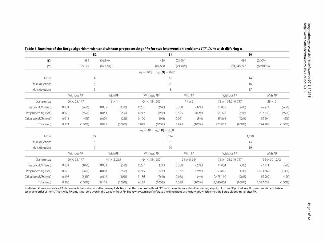
In the most demanding case (n/|D| 1), the Bergealgorithm with preprocessing identified 1,720 MCSs inless than 30 minutes in the large E0 model with its 124million EMs (see Table 5). Only 1% of the computation

time was used for the Berge algorithm. Ninety-four per-cent of the computation is spent on preprocessing. Afterpreprocessing the initial system of 124 million EMs wasreduced to approximately 300,000 modes. In all testedcases with enhanced preprocessing, reading EMs and pre-processing took at least 90% of the total computation time.We repeated the same simulation without preprocessing.While the total runtime with and without preprocessingis comparable if only a few MCSs are found, the runtimesavings in MCS calculation more than outweigh the run-time losses due to preprocessing if many MCSs solve anintervention problem. To emphasize this point we showthe total runtime as function of the number of MCSs forFigure 3 in the Additional file 2: Figure S1.

Finally in Table 6 we show several examples from the lit-erature, which can be easily and efficiently solved by eithermethod. As a comparison we have also listed runtimesusing the current version (version 2012.1) of CellNetAna-lyzer (CNA) [32]. CNA uses a MATLAB implementationof the Berge algorithm. However, its preprocessing capa-bilities are less developed. That is why both programs, ourBerge-algorithm and BIP, outperform CNA in all instancesby at least one order of magnitude. Note however thatCNA uses a MATLAB script, while our programs areimplemented in C. A significant part of the performancedifference may therefore be attributed to the slower per-formance of MATLAB compared to native executableswritten in C.

10-2

10-1

100

101

102

103

104

105

106

1 10 100 1000 10000

10-3

10-2

10-1

100

101

102

103

104

runt

ime

/ [se

c]

n

1 sec

1 min

1 hour

1 day

1 week

10-3

10-2

10-1

100

101

102

103

104

1 10 100 1000 1000010-2

10-1

100

101

102

103

104

105

106

runt

ime

/ [m

in]

runt

ime

/ [se

c]

n

1 sec

1 min

1 hour

1 day

1 week

Figure 3 Runtime for the Berge algorithm (left panel) and the BIP (right panel) for the models E2 (red) and E1 (blue), respectively. Theruntimes for preprocessing (circles) and calculating MCSs are plotted as function of n. n is the lower bound of desired EMs, which must survive theintervention. Table 4 gives the size of the intervention problem for both models. As the trend is clearly visible, we did not evaluate the BIP for n < 80.

Jungreuthmayeretal.BM

CBioinform

atics2013,14:318

Page8

of12http

://ww

w.b

iomedcentral.com

/1471-2105/14/318

Table 5 Runtime of the Berge algorithm with and without preprocessing (PP) for two intervention problems I(T , D, n) with differing nE2 E1 E0

|D| 489 (0.88%) 489 (0.10%) 489 (0.00%)

|T | 55,177 (99.12%) 484,680 (99.90%) 124,340,727 (100.00%)

n1 = 400; n1/|D| = 0.82

MCSs 4 11 44

Min. deletions 5 8 16

Max. deletions 5 8 17

Without PP With PP Without PP With PP Without PP With PP

System size 60 × 55, 177 13 × 1 64 × 484, 680 17 × 3 75 × 124, 340, 727 28 × 6

Reading EMs (sec) 0.031 (26%) 0.035 (43%) 0.281 (26%) 0.308 (37%) 71.858 (24%) 76.274 (26%)

Preprocessing (sec) 0.078 (65%) 0.044 (55%) 0.717 (65%) 0.495 (60%) 194.328 (64%) 202.539 (69%)

Calculate MCSs (sec) 0.011 (9%) 0.001 (2%) 0.100 (9%) 0.021 (3%) 35.866 (12%) 15.294 (5%)

Total (sec) 0.121 (100%) 0.081 (100%) 1.099 (100%) 0.823 (100%) 302.053 (100%) 294.108 (100%)

n2 = 40; n2/|D| = 0.08

MCSs 72 274 1,720

Min. deletions 5 6 14

Max. deletions 7 10 19

Without PP With PP Without PP With PP Without PP With PP

System size 60 × 55, 177 47 × 2, 295 64 × 484, 680 51 × 8, 664 75 × 124, 340, 727 62 × 321, 272

Reading EMs (sec) 0.031 (10%) 0.033 (25%) 0.277 (7%) 0.308 (20%) 71.084 (3%) 77.771 (5%)

Preprocessing (sec) 0.078 (26%) 0.083 (65%) 0.715 (17%) 1.162 (76%) 193.805 (7%) 1,493.367 (94%)

Calculate MCSs (sec) 0.196 (64%) 0.012 (10%) 3.136 (76%) 0.068 (4%) 2,475.110 (90%) 15.909 (1%)

Total (sec) 0.306 (100%) 0.128 (100%) 4.129 (100%) 1.539 (100%) 2,740.004 (100%) 1,587.053 (100%)

In all cases D are identical and T chosen such that it contains all remaining EMs. Note that the columns “without PP” state the runtimes without performing step 1 to 4 of our PP procedures. However, we still sort EMs inascending order of norm. This is why PP-time is not zero even in the cases without PP. The row “system size” refers to the dimensions of the network, which enters the Berge-algorithm, i.e. after PP.

Jungreuthmayer et al. BMC Bioinformatics 2013, 14:318 Page 9 of 12http://www.biomedcentral.com/1471-2105/14/318

Table 6 Runtime analysis for the Berge algorithm and BIP using several examples from the literature with differentdesign objectives

Runtime (sec)

Organism Objective |D| |T| # MCS Min. � Max. � Berge BIP CNA

E. coli [16] (anaerobic) ethanol 12 4,998 1,048 6 9 0.011 0.287 2.83

E. coli [16] (aerobic) ethanol 12 429,264 55,488 11 15 0.883 2.174 547.61

E. coli [15] (anaerobic) isobutanol 7 5,615 760 7 10 0.011 0.233 2.69

E. coli [33] (anaerobic) n-butanol 7 7,341 2,280 7 10 0.015 0.226 3.43

Both algorithms use all preprocessing procedures. For comparison we also use the program package CellNetAnalyzer [32] which uses a MATLAB script of the Bergealgorithm. (Abbreviations: #MCS, number of MCS; min. �, minimal number of deletions; max. �, maximal number of deletions; CNA, CellNetAnalyzer).

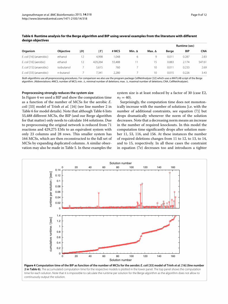
Preprocessing strongly reduces the system sizeIn Figure 4 we used a BIP and show the computation timeas a function of the number of MCSs for the aerobic E.coli [33] model of Trinh et al. [16] (see line number 2 inTable 6 for model details). Note that although Table 6 lists55,488 different MCSs, the BIP (and our Berge algorithmfor that matter) only needs to calculate 164 solutions. Dueto preprocessing the original network is reduced from 71reactions and 429,275 EMs to an equivalent system withonly 23 columns and 28 rows. This smaller system has164 MCSs, which are then reconstructed to the full set ofMCSs by expanding duplicated columns. A similar obser-vation may also be made in Table 5. In these examples the

system size is at least reduced by a factor of 30 (case E2,n2 = 40).

Surprisingly, the computation time does not monoton-ically increase with the number of solutions [i.e. with thenumber of additional constraints, see equation (7)] butdrops dramatically whenever the norm of the solutiondecreases. Note that a decreasing norm means an increasein the number of required knockouts. In this model thecomputation time significantly drops after solution num-ber 11, 53, 116, and 156. At these instances the numberof required deletions changes from 11 to 12, to 13, to 14,and to 15, respectively. In all these cases the constraintin equation (7e) decreases too and introduces a tighter

0

0.2

0.4

0.6

0.8

1

1.2

1.4

0 20 40 60 80 100 120 140 160

cum

ulat

ive

runt

ime

/ [se

c]

Solution number

0

0.02

0.04

0.06

0.08

0.1

0.12

0.14 0 20 40 60 80 100 120 140 160

runt

ime

per

solu

tion

/ [se

c]

Solution number

Figure 4 Computation time of the BIP as function of the number of MCSs for the aerobic E. coli [33] model of Trinh et al. [16] (line number2 in Table 6). The accumulated computation time for the respective models is plotted in the lower panel. The top panel shows the computationtime for each solution. Note that it is impossible to calculate the runtime per solution for the Berge algorithm as the algorithm does not allow tocontinuously output the solution.

Jungreuthmayer et al. BMC Bioinformatics 2013, 14:318 Page 10 of 12http://www.biomedcentral.com/1471-2105/14/318

bound on the system. This allows the solver’s internal pre-processing to more efficiently compress the system, whichin turn brings down the computation time. If, however,the norm of the solution does not change then the com-putation time scales approximately exponentially with thenumber of MCSs. This behavior is expected as each solu-tion adds a new constrain to the system, which makes itharder to solve.

DiscussionRecently cMCSs have been introduced to predict opti-mal intervention strategies in order to achieve an arbitrarymetabolic objective [11]. Two algorithmic approacheshave been published for their calculation [10,11]. Here weshowed that both methods are equivalent. We addressedthe numerical efficiency of both methods in typical designproblems and found that in terms of runtime the Bergealgorithm is superior compared to BIP.

It may appear as a surprise that the Berge algorithmperforms so well even for the large cases presented inthis study, especially since the Berge method is knownfor its unfavorable performance in huge networks [34].However, here we showed that efficient preprocessing candramatically reduce the size of the networks. The adaptedBerge algorithm could then be run on the reduced sys-tems. Apparently, for small systems the Berge algorithm iseffective.

The importance of preprocessing in the calculation ofMCSs has been stressed earlier [23]. The preprocessingstrategies introduced herein focus especially on the addi-tional constraints posed by cMCSs, whereas [23] dealtonly with (unconstrained) MCSs. We were able to showthat our implementation outperforms the currently avail-able tool for computing (c)MCSs (see Table 6). The per-formance gain can be attributed to both the improvedpreprocessing and the efficient implementation in C.Herein we used standard preprocessing routines, whichare frequently applied in BIP [29]. Extensive literatureon preprocessing in binary and integer programming isavailable, see for instance Savelsbergh [35] for a good sum-mary of basic ideas. Since cMCSs can be stated as a BIP,these methods are readily adoptable. However, due to thealgorithmic complexity of BIP (solving numerous linearoptimizations as part of one BIP, etc.), a full enumerationbased on BIP seems not be competitive compared to theBerge algorithm (see Figure 3). Rather the usage of BIPpreprocessing rules followed by the Berge algorithm tocalculate cMCSs is suggested as an optimal computationstrategy.

The efficiency of preprocessing is dependent on theimposed design criterion. In the worst case the set ofdesired modes is empty (D = ∅) and T contains all EMsof a network. This situation corresponds to unconstrainedMCSs and thus to a full dualization of the hypergraph

spanned by the target modes. Except for step 4, none ofour preprocessing routines then provides an advantageand other solvers may be more appropriate [34]. Howeversuch cases are not relevant in the context of metabolicengineering, where we want to optimize favorable func-tionality. To fully utilize the potential of preprocessing theratio n/|D| should be close to one. This means that manyessential reactions will be removed from the system, andas a result of that many supersets will be detected, too.However, in practice it may suffice if only a few EMs outof the set of desired modes survive, i.e. n/|D| 1. Still,preprocessing provides a significant performance gain asindicated in Table 5. The runtime costs of preprocess-ing will be outweighed by the savings in MCS calculation,if the intervention problem has many solutions. In prac-tice, preprocessing will therefore be favorable, as typicalapplications have a few thousand solutions (see Table 6).

In our paper [10] we used weights in the objective func-tion of the BIP to take experimental difficulties in thedeletion of reactions into account. For instance, somereactions cannot be deleted as they are driven by diffu-sion, rather than catalyzed by an enzyme. Other reactions,on the other hand, may require the deletion of multiplegenes as they are catalyzed by different enzymes in paral-lel. By an appropriate choice of the weights in the objectivefunction BIP is able to predict the experimentally easiestdeletion strategies first [10]. However, in the preprocess-ing procedures above we did not consider weights in theobjective function. Identifying particular solutions in thecomplete list of MCSs has to be done in a separate post-processing step (for example by appropriately sorting theoutput, which can be done quite fast). Thus even withan additional post-processing step our implementation ofBerge’s algorithm will be faster than BIP. Note howeverthat the integration of regulatory information into thecMCS framework is a unique feature of the BIP approach[10].

Both methods, the Berge algorithm as well as BIP, stillshow room for computational improvements. In the caseof the Berge algorithm the computational bottleneck sitsin the filtering of potential MCSs to determine if theyare, in fact, true MCSs and not supersets of true MCSs[23]. Generating new MCS-candidates, however, is veryquick. Therefore ways of enhancing the superset-filteringprocedure will be the scope of future work.

One disadvantage of the Berge algorithm is its inabilityto predict MCSs continuously during the runtime. Duringexecution all MCSs remain candidate-MCSs. Only upontermination, when the minimality of all candidate MCSshas been checked against each other, candidate-MCSsbecome MCSs and can be outputted. Thus, even if wewere interested in only one solution, the Berge algorithmwill – in general – return more than one MCS upon ter-mination. However, other solvers are available [34]. Their

Jungreuthmayer et al. BMC Bioinformatics 2013, 14:318 Page 11 of 12http://www.biomedcentral.com/1471-2105/14/318

adaption for the current situation is the scope of furtherwork.

BIP on the other hand, is able to predict a single solu-tion without the need to enumerate all. In fact, due to theoptimization principle only one MCS with a smallest orlargest number of deletions can be calculated. In Figure 4we illustrated the runtime per solution as function ofthe number of MCSs. The drop in runtime after cer-tain solutions indicates that more advanced preprocessingprocedures may further reduce the runtime significantly.In fact, our preprocessing focused on standard procedureslike variable fixing. More advanced methods will furtherreduce the runtime for both the Berge algorithm and theBIP. Additionally we used GUROBI, a commercially avail-able multi-purpose optimization toolbox, to solve the BIP.However, a specialized knapsack solver may potentiallyboost the performance.

ConclusionsWe predicted minimal metabolic intervention strate-gies in typical metabolic engineering problems usingtwo different methods (an adapted Berge algorithm anda BIP). We investigated the numerical performance ofthese approaches. Both methods significantly profitedfrom the enhanced preprocessing procedures developedhere. Under the tested conditions, our implementationof Berge’s algorithm performed best even outperformingother, currently available software.

Additional files

Additional file 1: tar gzipped archive of the SBML files for the modelsE0, E1, and E2.

Additional file 2: Total runtime with and without preprocessing forthe Berge algorithm.

AbbreviationsBIP: Binary integer program; cMCS: Constrained minimal cut set; CNA:CellNetAnalyzer; EM: Elementary mode; MCS: Minimal cut set; PP:Preprocessing.

Competing interestsThe authors declare that they have no competing interests.

Authors’ contributionsCJ implemented the algorithms and participated in the design of the study.GN coded the models and helped in running the analysis. SK participated inthe design of the study. JZ conceived of the study, and participated in itsdesign and coordination. CJ, SK and JZ wrote the manuscript. All authors readand approved the final manuscript.

AcknowledgementsC.J., G.N., and J.Z. gratefully acknowledge the support by the Federal Ministryof Economy, Family and Youth (BMWFJ), the Federal Ministry of Traffic,Innovation and Technology (bmvit), the Styrian Business Promotion AgencySFG, the Standortagentur Tirol and ZIT - Technology Agency of the City ofVienna through the COMET-Funding Program managed by the AustrianResearch Promotion Agency FFG.S.K. acknowledges funding by the German Federal Ministry of Education andResearch(e:Bio - 0316183D) and by the Ministry of Education and Research ofSaxony-Anhalt (Research Center “Dynamic Systems: Biosystems Engineering”).

Author details1Austrian Centre of Industrial Biotechnology, Vienna, Austria. 2Department ofBiotechnology, University of Natural Resources and Life Sciences, Vienna,Austria. 3Max Planck Institute for Dynamics of Complex Technical Systems,Magdeburg, Germany.

Received: 18 January 2013 Accepted: 30 October 2013Published: 6 November 2013

References1. Lee JW, Na D, Park JM, Lee J, Choi S, Lee SY: Systems metabolic

engineering of microorganisms for natural and non-naturalchemicals. Nat Chem Biol 2012, 8(6):536–546.

2. Xu P, Ranganathan S, Fowler ZL, Maranas CD, Koffas MA: Genome-scalemetabolic network modeling results in minimal interventions thatcooperatively force carbon flux towards malonyl-CoA. Metab Eng2011, 13(5):578–587.

3. Zomorrodi AR, Suthers PF, Ranganathan S, Maranas CD: Mathematicaloptimization applications in metabolic networks. Metab Eng 2012,14(6):672–686.

4. Kim J, Reed J: OptORF: Optimal metabolic and regulatoryperturbations for metabolic engineering of microbial strains.BMC Syst Biol 2010, 4:53.

5. Choi HS, Lee SY, Kim TY, Woo HM: In Silico identification of geneamplification targets for improvement of lycopene production.Appl Environ Microbiolo 2010, 76(10):3097–3105.

6. Ranganathan S, Suthers PF, Maranas CD: OptForce: An optimizationprocedure for identifying all genetic manipulations leading totargeted overproductions. PLoS Comput Biol 2010, 6(4):e1000744.

7. Pharkya P, Burgard AP, Maranas CD: OptStrain: A computationalframework for redesign of microbial production systems. GenomeRes 2004, 14(11):2367–2376.

8. Burgard AP, Pharkya P, Maranas CD: Optknock: A bilevel programmingframework for identifying gene knockout strategies for microbialstrain optimization. Biotechnol Bioeng 2003, 84(6):647–657.

9. Segrè D, Vitkup D, Church GM: Analysis of optimality in natural andperturbed metabolic networks. Proc Natl Acad Sci 2002,99(23):15112–15117.

10. Jungreuthmayer C, Zanghellini J: Designing optimal cell factories:Integer programing couples elementary mode analysis withregulation. BMC Syst Biol 2012, 6:103.

11. Hädicke O, Klamt S: Computing complex metabolic interventionstrategies using constrained minimal cut sets. Metab Eng 2011,13(2):204–213. http://www.ncbi.nlm.nih.gov/pubmed/21147248.

12. Schuster S, Fell DA, Dandekar T: A general definition of metabolicpathways useful for systematic organization and analysis ofcomplex metabolic networks. Nat Biotech 2000, 18(3):326–332.http://dx.doi.org/10.1038/73786.

13. Schuster S, Dandekar T, Fell DA: Detection of elementary flux modes inbiochemical networks: a promising tool for pathway analysis andmetabolic engineering. Trends Biotechnol 1999, 17(2):53–60.http://www.ncbi.nlm.nih.gov/pubmed/10087604.

14. Becker J, Zelder O, Häfner S, Schröder H, Wittmann C: From zero to hero–design-based systems metabolic engineering of Corynebacteriumglutamicum for L-lysine production. Metab Eng 2011, 13(2):159–168.

15. Trinh CT, Li J, Blanch HW, Clark DS: Redesigning Escherichia colimetabolism for Anaerobic production of Isobutanol. Appl EnvironMicrobiol 2011, 77(14):4894–4904.

16. Trinh CT, Unrean P, Srienc F: Minimal Escherichia coli cell for the mostefficient production of ethanol from Hexoses and Pentoses. ApplEnviron Microbiol 2008, 74(12):3634–3643. http://aem.asm.org/content/74/12/3634.abstract.

17. Unrean P, Trinh CT, Srienc F: Rational design and construction of anefficient E. coli for production of diapolycopendioic acid. Metab Eng2010, 12(2):112–122.

18. Xu X, Cao L, Chen X: Elementary flux mode analysis for optimizedethanol yield in anaerobic fermentation of glucose withsaccharomyces cerevisiae. Chin J Chem Eng 2008, 16:135–142.

19. Driouch H, Melzer G, Wittmann C: Integration of in vivo and in silicometabolic fluxes for improvement of recombinant proteinproduction. Metab Eng 2012, 14:47–58.

Jungreuthmayer et al. BMC Bioinformatics 2013, 14:318 Page 12 of 12http://www.biomedcentral.com/1471-2105/14/318

20. Zanghellini J, Ruckerbauer DE, Hanscho M, Jungreuthmayer C:Elementary flux modes in a nutshell: properties, calculation andapplications. Biotechnol J 2013, 8(9):1009–1016.

21. Trinh C, Wlaschin A, Srienc F: Elementary mode analysis: a usefulmetabolic pathway analysis tool for characterizing cellularmetabolism. Appl Microbiol Biotechnol 2009, 81(5):813–826.

22. Berge C: Hypergraphs: Combinatorics of Finite Sets. (North-Hollandmathematical library: Volume 45.) Amsterdam: Elsevier SciencePublishers; 1989.

23. Haus UU, Klamt S, Stephen T: Computing knock-out strategies inmetabolic networks. J Comput Biol 2008, 15(3):259–268.

24. Jungreuthmayer C, Ruckerbauer DE, Zanghellini J: regEfmtool:Speeding up elementary flux mode calculation usingtranscriptional regulatory rules in the form of three-state logic.Biosystems 2013, 113:37–39.

25. Jevremovic D, Trinh CT, Srienc F, Sosa CP, Boley D: Parallelization ofNullspace algorithm for the computation of metabolic pathways.Parallel Comput 2011, 37(6-7):261–278.

26. Terzer M, Stelling J: Large-scale computation of elementary fluxmodes with bit pattern trees. Bioinformatics 2008, 24(19):2229–2235.

27. Kamp Av, Schuster S: Metatool 5.0: fast and flexible elementarymodes analysis. Bioinformatics 2006, 22(15):1930–1931.

28. Eiter T, Makino K, Gottlob G: Computational aspects of monotonedualization: A brief survey. Discrete Appl Math 2008, 156(11):2035–2049.

29. Chen DS, Batson RG, Dang Y: Applied Integer Programming: Modeling andSolution. Hoboken: John Wiley & Sons, Inc.; 2010.

30. Orth JD, Fleming RMT, Palsson BØ: Reconstruction and use of microbialmetabolic networks: the core escherichia coli metabolic model as aneducational guide. In EcoSal-Escherichia coli and Salmonella: Cellular andMolecular Biology. Edited by Böck A, Curtiss IIIR, Kaper JB, Karp PD,Neidhardt FC, Nyström T, Slauch JM, Squires CL, Ussery D. Washington:ASM Press; 2009:56–99. chapter 10.2.1.

31. Deutscher J: The mechanisms of carbon catabolite repression inbacteria. Curr Opin Microbiol 2008, 11(2):87–93.

32. Klamt S, Saez-Rodriguez J, Gilles E: Structural and functional analysis ofcellular networks with CellNetAnalyzer. BMC Syst Biol 2007, 1:2.

33. Trinh CT: Elucidating and reprogramming Escherichia colimetabolisms for obligate anaerobic n-butanol and isobutanolproduction. Appl Microbiol Biotechnol 2012, 95(4):1083–1094.

34. Murakami K, Uno T: Efficient algorithms for dualizing large-scalehypergraphs. arXiv:1102.3813 2011. http://arxiv.org/abs/1102.3813.

35. Savelsbergh MWP: Preprocessing and probing techniques for mixedinteger programming problems. ORSA J Comput 1994, 6(4):445–454.

doi:10.1186/1471-2105-14-318Cite this article as: Jungreuthmayer et al.: Comparison and improvement ofalgorithms for computing minimal cut sets. BMC Bioinformatics 2013 14:318.

Submit your next manuscript to BioMed Centraland take full advantage of:

• Convenient online submission

• Thorough peer review

• No space constraints or color figure charges

• Immediate publication on acceptance

• Inclusion in PubMed, CAS, Scopus and Google Scholar

• Research which is freely available for redistribution

Submit your manuscript at www.biomedcentral.com/submit