Comparing responses of freshwater fish and invertebrate community integrity along multiple environmental gradients

Page 1

Ci

ASa

b

c

a

ARRA

KBSBCLMO

1

ioilunas2sd

h1

Ecological Indicators 43 (2014) 215–226

Contents lists available at ScienceDirect

Ecological Indicators

j o ur na l ho me page: www.elsev ier .com/ locate /eco l ind

omparing responses of freshwater fish and invertebrate communityntegrity along multiple environmental gradients

nne Pilièrea,∗, Aafke M. Schippera, Anton M. Breurea,b, Leo Posthumab, Dick de Zwartb,cott D. Dyerc, Mark A.J. Huijbregtsa

Radboud University Nijmegen, Institute for Water and Wetland Research, P.O. Box 9010, 6500 GL Nijmegen, The NetherlandsNational Institute for Public Health and the Environment (RIVM), PO Box 1, 3720 BA Bilthoven, The NetherlandsThe Procter & Gamble Company, P.O. Box 599, Cincinnati A., Ohio 45202, United States

r t i c l e i n f o

rticle history:eceived 3 June 2013eceived in revised form 2 February 2014ccepted 10 February 2014

eywords:iotic integritytressor–response relationshipsoosted Regression Treesommunity concordanceotic ecosystemsultimetric indiceshio

a b s t r a c t

Multimetric indices of biotic integrity provide a quantitative measure of biological quality and have beendeveloped for several taxonomic groups. Community integrity for fish is typically represented by the mul-timetric Index of Biotic Integrity (IBI), while for macroinverterates the Invertebrate Community Index(ICI) can be applied. Given the considerable sampling efforts required for biomonitoring, it is important toknow the extent to which indices based on particular taxonomic groups respond differently to (anthro-pogenic) stressors in the environment. The three goals of our study were (1) to assess the concordanceof freshwater fish and macroinvertebrate communities, (2) to derive stressor–response relationships forIBI and ICI pertaining to multiple environmental factors and (3) to compare the responses of IBI and ICI tothese environmental factors in the state of Ohio (USA). We used a database containing abiotic as well asbiotic information for 545 local catchments located across Ohio (USA). Our 22 environmental factors cov-ered physiography, water chemistry, physical habitat quality and toxic pressure. Concordance betweenthe fish and invertebrate communities was assessed using a Mantel test. Response patterns of IBI and ICI toeach of the environmental factors were analyzed by constructing stressor–response curves with Boosted

Regression Trees (BRT). Fish community integrity was primarily related to physical characteristics ofthe stream (channel- and riffle quality) and latitude, whereas invertebrate community integrity mainlyresponded to the phosphorus concentration. Response curves showed that the two indices respondedsimilarly to most of the water chemistry variables, while responses differed for physiographical andphysical habitat quality variables.

. Introduction

In biomonitoring, the environmental quality of a given sites judged from its species assemblages, based on knowledgef environment–biota relationships. In this context, multimetricndices of biotic integrity are widely used to evaluate the bio-ogical and thus environmental quality of a site. Integrity indicesse multiple characteristics of biotic communities (e.g., the rich-ess and or abundance of specific taxonomic or functional groups)nd measure their deviation from values observed in referenceites (Joy and De’ath, 2004; Weigel et al., 2006; Whittier et al.,

007). Reference sites are usually defined as the least disturbedites in a given ecoregion, and serve as the basis for evaluating theegree of anthropogenic disturbance of sites belonging to the same

∗ Corresponding author. Tel.: +31 0243652066.E-mail address: [email protected] (A. Pilière).

ttp://dx.doi.org/10.1016/j.ecolind.2014.02.019470-160X/© 2014 Elsevier Ltd. All rights reserved.

© 2014 Elsevier Ltd. All rights reserved.

ecoregion. Various biotic integrity indices exist, based on differ-ent taxonomic groups, such as fish, invertebrates, birds, terrestrialarthropods and wetland plant communities, and adapted to spe-cific geographic areas (Bryce et al., 2002; DeKeyser et al., 2003; Karrand Kimberling, 2003; Klemm et al., 2003; Joy and De’ath, 2004).Given the considerable investments in time and money requiredto conduct detailed field ecological assessments, an importantquestion is whether the biotic integrity of particular taxonomicgroups can be used to predict that of other groups, particularly inresponse to (anthropogenic) stressors in the environment (Heino,2010).

Predicting the composition and integrity of one group accord-ing to another’s requires strong community concordance, definedas the degree of similarity in assemblage structure patterns among

taxonomic groups (Paavola et al., 2006). Recently, several studieshave investigated community concordance among different tax-onomic groups used in ecological assessments, but they obtainedcontradicting results. For example, freshwater fish and invertebrate

Page 2

2 l Indic

ceRit2cm(Gtccbeail(Tittm

atcatdccBag(tmmRwnitb

2

btEdlww(Ewaad

16 A. Pilière et al. / Ecologica

ommunities appeared concordant in some studies and not in oth-rs (Paavola et al., 2006; Infante et al., 2009; Dolph et al., 2011;ooney and Bayley, 2012). Community concordance values were

nfluenced by the study’s spatial scale (Paavola et al., 2006) and byhe biological traits of the organisms of concern (Grenouillet et al.,008). Studies addressing the underlying causes of community con-ordance found that similarities in assemblage structure patternsay originate from similar responses to environmental gradients

e.g. Neff and Jackson, 2013), but also from biotic interactions (e.g.renouillet et al., 2008; Larsen et al., 2012). Most studies conclude

hat the concordance between fish and invertebrates is not suffi-ient to use those two taxa as surrogates for each other, even inase of strong concordance, because the two groups are not driveny the same environmental factors (Grenouillet et al., 2008; Infantet al., 2009; Dolph et al., 2011; Padial et al., 2012). However, studiesddressing differences in environmental drivers between fish andnvertebrates typically quantify these in terms of the overall corre-ation between the response and a particular environmental drivere.g. Bedoya et al., 2011; Infante et al., 2009; Neff and Jackson, 2013).hus, these studies do not provide detailed information on changesn the responses along the environmental gradients. Such informa-ion is especially relevant as it would allow to identify where onhe environmental gradient management measures would be the

ost effective.The three goals of our study were (1) to assess the concord-

nce of freshwater fish and macroinvertebrate communities, (2)o derive stressor–response relationships for fish and invertebrateommunity integrity pertaining to multiple environmental factorsnd (3) to compare the environmental responses of fish and inver-ebrate community integrity in the state of Ohio (USA). Using aatabase containing biotic and abiotic information for 545 localatchments across the state of Ohio (USA), we first quantified theoncordance between fish and invertebrate communities usingray–Curtis dissimilarity matrices and a Mantel test. Then, wessessed changes in the integrity of the two communities along theradients of 22 environmental factors belonging to four categoriesphysiography, physical stream habitat, water chemistry and mix-ure toxic pressure). Community integrity was represented by the

ultimetric Index of Biotic Integrity (IBI) and the Invertebrate Com-unity Index (ICI) for the fish and the invertebrates, respectively.

esponses of IBI and ICI to environmental factors were analyzedith Boosted Regression Trees (BRT). We determined the mag-itude of the effect of each environmental predictor on the two

ndices, and extracted response curves for each environmental fac-or to visualize potential differences in environmental responsesetween IBI and ICI.

. Methods

The dataset used in our study is part of a database developedy a consortium of companies and institutes including The Proc-er & Gamble Co., the Dutch Institute for Public Health and thenvironment (RIVM) and Waterborne Environmental, Inc. Bioticata were available from 545 biomonitoring sites of the Ohio EPA

ocated across the state of Ohio (Fig. 1). Each biomonitoring siteas sampled once during the period 2000–2008. Local catchmentsere delineated based on the National Hydrography Dataset Plus

NHD Plus, USEPA and USGS, 2005), such that there was one OhioPA biomonitoring site within each catchment. Abiotic variables

ere measured within each local catchment during the same year

s biotic data. Below, we provide a brief description of the bioticnd abiotic variables included in our study. More details on theata collection and processing are given in Appendix A.

ators 43 (2014) 215–226

2.1. Biotic indices

Fish were sampled by either boat-mounted or wading elec-trofishing methods (Sportyak generator or long-line generator).The invertebrates were collected with Hester-Dendy artificial sub-strates and D-net kicks (Ohio EPA, 1989). Fishes were all identifiedat species level, while invertebrates were identified at species levelwhenever possible, else at genus or family level. Presence–absencedata were available for 736 invertebrate taxa and 129 fish taxa. Inaddition, the database contained two multimetric indices repre-senting the integrity of the fish and invertebrate communities. TheIndex of Biotic Integrity (IBI) measures the biological integrity ofthe fish community by quantifying the deviation from communi-ties observed in minimally disturbed reference sites. It is composedof 12 submetrics describing structural (e.g., species richness or pro-portion of individuals from given taxonomic groups) and functional(e.g., pollution-tolerant taxa, trophic groups) aspects of the fishcommunity. The raw values of the submetrics, as obtained fromfield data, are assigned scores according to the degree of deviationfrom the values expected at a reference site, located in a stream ofsimilar size in a similar ecoregion. The reference sites for each of thefive ecoregions of Ohio were defined by expert judgment as siteswith minimum human influence (Ohio EPA, 1987). Each metric cantake a value of 1, 3 or 5; the higher the deviation from referenceconditions, the lower the score. The overall IBI score is obtainedby summing all submetric scores and ranges from 12 (integrityhighly deviating from reference conditions) to 60 (integrity similarto reference conditions). The Invertebrate Community Index (ICI) isquantified according to a similar procedure. It includes 10 submet-rics which can take values of 0, 2, 4 or 6. Hence, the overall indexranges from 0 to 60 (Ohio EPA, 1987). For reasons of comparability,we rescaled both indices to a 0–100 range.

2.2. Environmental predictors

The 22 environmental predictors we included belong to fourcategories: physiography, physical habitat quality, water chem-istry and toxic pressure (Table 1). Watershed area was used asa surrogate for discharge volume, altitude accounted for climaticparameters and slope for flow velocity. We included latitude andlongitude to account for spatial autocorrelation, large-scale bio-geographical patterns and unmeasured but potentially relevantenvironmental variables. Examples include precipitation or anthro-pogenic factors like impervious cover of the soil, which influencesthe hydrological regime. The stream physical habitat quality wasexpressed by the seven submetrics of the Qualitative Habitat Eval-uation Index (QHEI; Ohio EPA, 2006) (Table 1). The QHEI is amultimetric index evaluating the physical macrohabitat quality inrunning waters. Its submetrics are related to particular character-istics of the stream habitat, such as substrate quality or channelmorphology. Based on expert judgment, scores are assigned toeach submetric, which are then summed to arrive at an overallscore ranging from 0 (poorest quality) to 100 (maximum qual-ity). Nine water chemistry predictors were included: pH, oxygendemand (biological and chemical), nutrient concentrations (totalnitrogen and total phosphorus), total dissolved and total suspendedsolids, conductivity and hardness (Table 1). Toxic pressure wasexpressed as the multi-substance Potentially Affected Fraction ofspecies (msPAF) due to the combined impacts of several groupsof toxicants: industrial products, household products, synthetic

estrogens and pharmaceuticals. The msPAF was calculated basedon environmental concentrations of the substances combined withbioavailability assessments, ecotoxicity data and mixture toxicitymodels (Posthuma et al., 2002; De Zwart et al., 2006; Posthuma

Page 3

A. Pilière et al. / Ecological Indicators 43 (2014) 215–226 217

Table 1Description of the environmental predictors and response variables, with their mean and range across the 545 sampled sites.

Unit Mean Minimum 1st quartile 2nd quartile 3rd quartile Maximum

Environmental factorsPhysiography

Watershed area upstream ofthe sampled point

km2 263.4 1.0 28.0 67.5 213.0 7995.0

Latitude degree 40.2 38.7 39.6 40.1 40.9 41.8Longitude degree −82.8 −84.8 −83.7 −82.9 −81.9 −80.7Altitude m 248.2 138.9 212.0 243.0 286.0 370.5Average slope of the

catchment% 5.5 0.5 2.5 3.9 6.7 31.6

Physical habitat quality (metrics of the Ohio-specific qualitative habitat evaluation index)Channel – 13.9 4.0 12.0 14.5 16.5 20.0Cover – 13.5 1.0 12.0 14.0 16.0 21.0Gradient metric – 8.0 2.0 6.0 8.0 10.0 10.0Pool – 9.0 2.0 7.6 9.3 11.0 12.0Riffle – 3.8 −1.0 2.0 4.0 6.0 8.0Riparian – 6.1 1.0 5.0 6.0 7.0 10.0Substrate – 13.9 −1.5 12.0 14.5 16.5 21.5

Water chemistryBiological oxygen demand on

five daysmg/L 2.5 1.0 1.0 1.0 3.3 21.0

Chemical oxygen demand mg/L 27.1 5.0 16.0 22.0 30.0 258.0Specific conductance �S/cm 815.1 122.0 599.0 734.0 909.0 5060.0Hardness (total CaCO3

concentration)mg/L 324.1 51.0 243.0 318.0 373.0 1700.0

Total nitrogen concentration mg/L 1.0 0.1 0.5 0.7 1.0 33.5Total phosphorus

concentrationmg/L 3.5 0.0 0.1 0.2 0.4 128.0

pH SU 7.9 3.2 7.7 7.9 8.1 9.7Total dissolved solids mg/L 515.0 86.0 362.0 452.0 582.0 3910.0Total suspended solids mg/L 63.1 2.5 12.0 27.0 63.0 1590.0

Toxic pressureMulti-substances potentially

affected fraction of speciesfraction 0.1 0.0 0.0 0.0 0.1 0.9

Biological endpointsOhio-specific index of

biological integrity for fishcommunities

– 43.1 12.0 37.0 45.0 50.4 58.0

Ohio-specific index of – 42.0 0.0 37.3 44.0 50.0 60.0

aa

2

isusnptb

mB(F(neaadal

biological integrity formacroinvertebratecommunities

nd De Zwart, 2006). More details about the msPAF calculationsre provided in Appendix A.

.3. Statistical analyses

We assessed the concordance of the freshwater fish andnvertebrate communities with a Mantel (1967) test applied to dis-imilarity matrices derived from the presence–absence data. Wesed the Bray–Curtis distance as a measure of dissimilarity amongites and Pearson’s correlation coefficient as a measure of commu-ity concordance (Grenouillet et al., 2008). We used a Monte-Carloermutation test with 5000 repetitions to assess the significance ofhe Mantel test results. In addition, we calculated the associationetween ICI and IBI with Pearson’s correlation coefficient.

To investigate the responses of IBI and ICI to the environ-ental predictors, we applied Boosted Regression Trees (BRT).

RT are an improvement of classification and regression treesDe’ath and Fabricius, 2000). The principle of BRT is described byriedman (2001), Friedman and Meulman (2003) and Elith et al.2008). BRT constitute a relatively new machine-learning tech-ique able to model a large variety of ecological responses (Knudbyt al., 2010; Williams and Poff, 2006; Snelder et al., 2012). Theirdvantages include the stability of the model in case of outliers,

utomatic fitting of predictors’ interactions, and ability to han-le missing values (Elith et al., 2008). They provide an efficientpproach to investigate biota-environment relationships in eco-ogical databases (Cappo et al., 2005; Hopkins and Whiles, 2011;

Leclere et al., 2011; Waite et al., 2012). BRT determine the optimalprediction of a response variable given a set of predictors, and therelative importance of each predictor in predicting the response. Inaddition, BRT provide information on the marginal effect of eachpredictor, as they generate matrices containing predictor valuesacross the gradient and the associated response values given aver-aged influences of all other predictors. This information can beused to derive predictor–response curves that illustrate the direc-tion (positive or negative) and shape (linear, unimodal, multimodal,presence of thresholds) of the relationship between a response anda particular predictor.

Parameterization of the BRT models requires to set values fordifferent parameters. The BRT algorithm will automatically stopadding trees when the predictive power of the overall model nolonger improves. The learning rate (�) controls the gain in predic-tive power to achieve at each step so that addition of trees is allowedto go on. The smaller the learning rate, the lower the threshold, andthe higher the final number of trees. The tree complexity repre-sents the maximum number of splits in each individual tree, whichcorresponds to the maximum order of predictor interactions thatcan be fitted by the model, provided the data support the fitting ofsuch interactions. Finally, the bag-fraction represents the fractionof the dataset to be randomly drawn and used for model training

at each step. For more details on BRT functioning and parameter-ization, see Elith et al. (2008). For each BRT model, we selectedoptimal parameter values by systematically varying (i) the learn-ing rate, taking the values 0.001, 0.005, 0.01 and 0.05, (ii) the tree

Page 4

2 l Indicators 43 (2014) 215–226

ctbo4vWtIwirTrttadb

psdast(

Q

wvs

vetPr

Rc(B

3

fl(wefpcnw(

mcdtt

Table 2Results of the Boosted Regression Trees Models. The contribution of each environ-mental predictor is expressed as the contribution to the overall predictive power ofthe best BRT model for the biotic endpoint of concern. Contributions of at least 5%and corresponding predictors are depicted in bold. Partial dependency plots for allpredictors are shown in Fig. 2.

Biotic endpoints

IBI ICIq2 q2

PhysiographyWatershed area (km2) 1.1 1.7Latitude (degree) 5.9 2.1Longitude (degree) 2.6 0.9Altitude (m) 1.9 0.8Slope 1.5 1.4

Physical habitat qualityChannel 6.6 1.6Cover 1.1 0.7Gradient 0.3 0.9Pool 2.4 0.7Riffle 8.1 1.9Riparian 0.3 0.9Substrate 1.8 2.4

Water chemistryBOD5 (mg/L) 0.2 1.8COD (mg/L) 0.7 1.2Conductance (mS/cm) 3.3 1.1Hardness (mg/L CaCO3) 1.3 1.2N (mg/L) 1.6 2.0P (mg/L) 5.4 4.9pH (SU) 2.1 2.6Total dissolved solids (mg/L) 1.6 1.2Total suspended solids(mg/L)

0.4 1.2

Toxic pressureMsPAF (%) 0.7 0.7

Total predictive power of themodel (%)

50.7 33.9

18 A. Pilière et al. / Ecologica

omplexity, taking the values 1–7, and (iii) the bag-fraction, takinghe values of 0.55, 0.65 and 0.75. For each of the two indices, we thusuilt 7 × 3 × 4 = 84 models, representing all possible combinationsf 10 different tree complexity values, 3 different bag-fractions, and

different learning rates. The maximum number of trees per indi-idual model was set at 50,000, and this number was never reached.e eliminated a posteriori the models based on fewer than 1000

rees, following the rule of thumb suggested by Elith et al. (2008).n order to prevent overfitting, each of the 84 models per index

as built following a ten-fold cross-validation procedure. Accord-ng to this procedure, 10 BRT models are built in parallel using 10andom subsets of the data, each comprising 9/10th of the dataset.he predictive performance of each of these models is tested on theemaining 1/10th of the dataset (i.e., the validation data), wherebyhe 10 validation datasets are mutually exclusive (i.e., each observa-ion is used for testing only once). The predictive power is assessedfter each addition of trees and addition of trees stops when the pre-ictive power no longer improves. The final BRT model is obtainedy averaging the predictive power and predictions of the 10 models.

The predictive power of the BRT models, assessed as the totalercentage of deviation explained, was given by the predictivequared correlation coefficient Q2 (Eq. (1)) of the regression of pre-icted values against observed ones (Legates and McCabe, 1999),veraged across the cross-validation models. For each index, weelected the ‘best’ model as the model with the highest predic-ive power among the 84 different combinations of parametersFriedman, 2001; Elith et al., 2008).

2 = 1 −∑N

i=1(ypred,i − yi)2

∑Ni=1(yi − ymean)2

(1)

here N represents the number of data points, ypred,i the predictedalue for point i, yi the observed value for point i of the validationet, and ymean the mean of observed values in the validation set.

The relative importance of a predictor for a particular responseariable was calculated by summing the deviation explained byach split the predictor was involved in, relative to the total devia-ion explained by the model, averaged across cross-validation sets.artial dependency plots illustrating single predictor–responseelationships were constructed based on the best model per index.

For all analyses we used the freely available statistical software version 2.14.0 (R Development Core Team, 2008). Communityoncordance was tested using functions from the vegan packageOksanen et al., 2013). BRT required the gbm package and additionalRT functions (Elith et al., 2008).

. Results

The Mantel test yielded a value of rM = 0.53 (p-value < 0.001)or the state-wide community concordance. The Pearson corre-ation between the two integrity indices, IBI and ICI, was r = 0.49p-value < 0.001). The IBI was on average higher than the ICI,ith respective average scores of 59.3 and 51.7. The BRT mod-

ls had a higher predictive power for the IBI (Q2 = 0.51) thanor the ICI (Q2 = 0.34, Table 2). The relative importance of theredictors differed between the fish and the invertebrates. Fishommunity integrity was mainly correlated to riffle quality, chan-el quality and latitude, while invertebrate community integrityas primarily correlated to phosphorus, pH and substrate quality

Table 2).According to the response curves, fish and invertebrate com-

unity integrity responded similarly to the majority of the water

hemistry parameters, with most curves having the same shapeespite differences in amplitude (Fig. 2). Yet, ICI was nega-ively correlated with BOD5, while IBI showed no response. Thewo groups responded differently to physiographical variables,

Standard deviation acrosscross-validation sets (%)

8.3 8.6

with curves showing different amplitudes (e.g., watershed area),different maxima (e.g., altitude) or different trends (e.g., latitude,slope). Differences were also observed in the responses to habitatquality metrics (Fig. 2). The IBI was positively correlated to chan-nel, pool and riffle scores, whereas ICI was less or not correlatedto these metrics. Finally, ICI showed a stronger response to bothriparian and substrate scores than IBI.

4. Discussion

4.1. Community concordance and index correlation

In our study, we observed a significant concordance betweenfish and invertebrate communities across the state of Ohio. Someauthors suggest however to focus on the value of concordancerather than on the significance (e.g. Heino, 2010), because thepermutation test used to assess the significance of the Manteltest results is increasingly likely to indicate significant concord-ance with an increasing number of samples. Our concordancevalue was slightly higher than what Heino (2010) defined as low(rM < 0.5), and well below the threshold of rM > 0.7 that was sug-gested for strong concordance. It was nevertheless higher thanthe values of concordance observed in several former studies (e.g.Grenouillet et al., 2008; Infante et al., 2009; Larsen et al., 2012;Padial et al., 2012). Several factors, however, make it difficult

to compare our results with former studies. For example, con-cordance values obtained from presence–absence data are mostlyhigher than values based on abundance data, as variability is highlyreduced by the transformation of continuous data into binary

Page 5

A. Pilière et al. / Ecological Indicators 43 (2014) 215–226 219

Fig. 1. Location of the biomonitoring locations (n = 545) across the state of Ohio (USA).

Fig. 2. Partial dependency plots illustrating the response of the IBI (black) and ICI (dotted gray) to each single environmental predictor. The x-axis represents the gradientof the predictor across the sampled sites. The y-axis represents the variation in the IBI and ICI in relation to the predictor of concern given averaged influences of the otherpredictors. For each predictor–response curve, the response values were transformed by subtracting the minimum from every value, so that the lowest point of the responsevariable across the predictor’s gradient was given the value 0.

Page 6

2 l Indic

vtsopmcFnc2c

4f

wartbBp

uiBaptooetwqcfittspqr

twTffnbwawofimtltw

m

in review). Apart from the altitude data, which we added to thedataset ourselves (see Physiography), all data used in our studywere retrieved from this database. The database was assembledfrom data collected by the US Environmental Protection Agency

20 A. Pilière et al. / Ecologica

ariables. Our community concordance value is indeed higherhan the abundance-based concordance values reported in severaltudies reviewed by Heino (2010). However, Larsen et al. (2012)bserved a much lower concordance than ours while also usingresence–absence data. The differences in the scale of the studyay also influence the observed concordance values, with larger

oncordance values observed at larger scales (Paavola et al., 2006).inally, the techniques used differ, as some authors first use ordi-ation techniques on the stream assemblage data before assessingommunity concordance (e.g. Dolph et al., 2011, Neff and Jackson,013). Our medium concordance value was in line with a mediumorrelation between IBI and ICI.

.2. Response patterns of fish and invertebrates to environmentalactors

The BRT analyses identified a few main predictors for each index,ith different rankings for IBI and ICI. Our predictor ranking results

re in line with previous studies indicating that the main envi-onmental drivers differ for fish and invertebrates, and especiallyhat fish are more impacted by physical habitat and invertebratesy water chemistry (e.g. Bae et al., 2011; Neff and Jackson, 2013).elow we discuss the relative importance of the predictors and theredictor–response curves for IBI and ICI per predictor group.

The physical habitat quality components together contributedp to 28% of the BRT model’s predictive power for the IBI. This is

n agreement with the results from Manolakos et al. (2007) andedoya et al. (2011) for Ohio. Bedoya et al. (2011) used clusternalysis to link IBI to various environmental factors and mentionedhysical habitat quality, including riffle and channel scores, amonghe main predictors of the IBI. Furthermore, the higher sensitivityf ICI to substrate and riparian quality also matches the findingsf Manolakos et al. (2007). Life-history traits of organisms mayxplain the different responses of the two groups to physical habi-at factors (Grenouillet et al., 2008). Benthic macroinvertebrates,hich are largely restricted to the stream bed, depend on substrate

uality, while fish also depend on the characteristics of the waterolumn habitats. Only one component metric of the IBI relates tosh with distinct substrate-dependent life-history strategies (i.e.he percentage of simple lithophilic species), which may explainhe low contribution of substrate quality to the IBI model. It wasuggested that the lower dispersal abilities of invertebrates com-ared to fish make them more sensitive to local factors, such asuality of the microhabitat, which is linked to the substrate andiparian submetrics (LeRoy Poff, 1997).

In our study, phosphorus concentration appeared as an impor-ant predictor for both invertebrate and fish community integrity,hile nitrogen had a smaller predictive power for both indices.

his is in contrast with the findings of Bedoya et al. (2011), whoound a higher contribution of nitrogen to the predictive poweror IBI and ICI compared to phosphorus. A difference in the tech-ique employed might explain this, as the sites clustering usedy those authors reduces the influence of extreme values, whichere not ignored in our case. In our study, the responses of IBI

nd ICI to other water chemistry predictors and to toxic pressureere comparable, both in terms of magnitude and in terms of shape

f the response curves. This goes against the commonly acceptednding that organisms with a smaller surface/volume ratio areore exposed and thus more sensitive to water chemistry parame-

ers and especially pollutants (Neumann et al., 2005). Possibly, thearge gradients of the chemical predictors in our study overcomehe differences in tolerance range between fish and invertebrates,

hich would appear on a more subtle gradient (Schipper et al.,

2010).The generally low contribution of geographical factors to our

odels can be explained by the index calculation processes. The

ators 43 (2014) 215–226

integrity indices values are obtained by comparison with the valuesobtained in reference sites (i.e., minimally disturbed sites) locatedin a similar ecoregion. The ecoregions in Ohio were defined in sucha way that they exhibit similar characteristics for several terrestrialvariables, including land surface form, land use, soil characteristicsand potential natural vegetation (Ohio EPA, 1987). Thus, theintegrity index calculation aims to assess the degree of anthro-pogenic disturbance by eliminating most of the natural backgroundvariation. The very low contribution of watershed area to our mod-els, while fish and invertebrates have been shown to be stronglyaffected by the longitudinal gradient in streams, indicates thatnational background variation is efficiently removed during indexvalue calculation. The high contribution of latitude is likely due tocorrelation with external factors not included in our study, such asland use or impervious cover of the soil.

4.3. Implications for biomonitoring and environmentalmanagement

Our results showed that fish and invertebrate communities inOhio streams are moderately concordant, which was in line withthe correlation between the biotic indices of integrity derived fromthose two groups. The results of our BRT models explained thosefindings, at least partly, by showing that the two taxonomic groupsdiffer in their sensitivities to specific environmental factors, notablyphysical habitat quality characteristics. The differences emphasizethat one taxonomic group cannot be directly used as surrogatefor another to assess the influence of environmental factors onoverall biotic integrity. In our case, similar responses to waterchemistry, however, suggest that it is possible to use only one ofthe two taxonomic groups for biomonitoring if water chemistry isthe focus. The differences in the predictor ranking between fish andinvertebrates imply that, depending on the taxa of concern, differ-ent priorities can be set concerning environmental managementmeasures: improving stream physical habitat quality (particularlypool, riffle and channel quality) for fish, and water chemistryparameters (particularly phosphorus), along with substrate qual-ity for invertebrates. Finally, our stressor–response curves showedthat not only the amplitude, but also the direction of the effect of apredictor can differ between taxonomic groups.

Acknowledgements

We would like to thank Dennies Mischne (Ohio EPA), CharlotteWhite-Hull (P&G-retired), Katherine Kapo (Waterborne Environ-mental, Inc.), and Christopher Holmes (Waterborne Environmental,Inc.) for providing us with the Ohio data.

Appendix A. Data collection and processing

The dataset used in our study is part of a database developed bya consortium of companies and institutes including The Procter &Gamble Co., the Dutch Institute for Public Health and the Environ-ment (RIVM) and Waterborne Environmental, Inc. (see Kapo et al.,

(USEPA), Ohio Environmental Protection Agency (Ohio EPA) andthe US Geological Survey (USGS). Local catchments form the basicgeographical unit of the dataset. Local catchments were delineatedbased on the National HydrographyDataset Plus (NHD Plus, USEPA

Page 7

l Indic

aici2iwrudottlwnp

B

ptsaEEmcb

JstTtstc(baatfllmhmIa

atiInimopnavs

A. Pilière et al. / Ecologica

nd USGS, 2005), such that there was one Ohio EPA biomonitor-ng site within each catchment. The dataset used in our studyomprised 545 local catchments with an average size of approx-mately 2 km2. Each local catchment was sampled once during the000–2008 period. Biotic data were collected from the biomonitor-

ng sites. The watershed area, latitude, longitude and altitude valuesere measured based on the biomonitoring locations. Other envi-

onmental variables were measured within the local catchmentpstream of the biomonitoring location. Thus, each entry of theataset corresponds to a local catchment, with all biotic and abi-tic variables having been measured within this catchment duringhe same year. If there were multiple measurements per catchment,he values were aggregated as described later into a single value perocal catchment. Some variables (physical habitat quality, slope)

ere not measured for every local catchment in the dataset. Theumber of local catchments with data available for each variable isrovided in Table A1.

iotic endpoints

Field data for fish and invertebrate communities for the timeeriod 2000–2007 were obtained from the Ohio EPA. Withinhe Ohio EPA’s Biological Monitoring and Assessment program,tatewide biosurveys to assess the ecological status of Ohio riversnd streams are conducted every 5–10 years (see for example OhioPA, 2012). The state of Ohio is divided into 25 hydrological units.ach year, five of those units are monitored by sampling approxi-ately 400–500 sites in total. Methods were designed to obtain as

omplete a picture of the community as possible, partial collectionseing insufficient for the IBI and ICI calculation (Ohio EPA, 1989a,b).

Fish and macroinvertebrate sampling took place between mid-une and end of September, in appropriate climatic conditions. Fishampling was conducted by either boat-mounted or wading elec-rofishing methods (Sportyak generator or long-line generator).he appropriate standardized sampling gear was used accordingo stream size, and two or three passes were conducted for eachite, with a minimum of three weeks interval in between to ensurehat communities have the time to recover from the perturbationaused by sampling. All fish species were identified at species levelOhio EPA, 1989a,b). The quantitative collection of macroinverte-rates was conducted primarily using multi-plates Hester-Dendyrtificial substrates. Artificial substrates are colonized instream for

period of six weeks, with special care given to the location ofhe artificial substrates and the physical instream conditions (e.g.ow velocity) to ensure comparable conditions and optimal col-

ection. In addition, a qualitative (presence-absence) collection ofacroinvertebrates with D-net kicks takes place in all the natural

abitats present instream at the sampled location. Voucher speci-ens are retained for laboratory identification (Ohio EPA, 1989a,b).

nvertebrates are identified at species level whenever possible, elset genus or family level.

The database includes abundance of 736 invertebrate taxand 129 fish taxa for all of the 545 biomonitoring sites. Further,he database contains two multimetric indices to represent thentegrity of freshwater communities: IBI and ICI. The Index of Bioticntegrity (IBI) measures the biological integrity of the fish commu-ity by quantifying the deviation from fish communities observed

n minimally disturbed reference areas. It is composed of 12 sub-etrics describing structural (e.g., species richness or proportion

f individuals from given taxonomic groups) and functional (e.g.,ollution-tolerant taxa, trophic groups) aspects of the fish commu-

ity. The raw values of the submetrics, as obtained from field data,re assigned scores according to the degree of deviation from thealue expected at a reference site, located in a stream of similarize in a similar geographic area with minimal human influence.

ators 43 (2014) 215–226 221

Each metric can take a value of 1, 3 or 5; the higher the devia-tion from reference conditions, the lower the score. The overall IBIscore is obtained by summing all submetric scores and ranges from12 (integrity highly deviating from reference) to 60 (reference-condition like integrity). The Invertebrate Community Index (ICI)is quantified according to a similar procedure. It includes 10 sub-metrics which can take values of 0, 2, 4 or 6: the overall index thusranges from 0 to 60 (Ohio EPA, 1989a,b).

Environmental variables

Physiography

The entire watershed area upstream of each biomonitoring loca-tion was delineated by identifying and aggregating all upstreamlocal catchments, including the catchment of the biomonitoringsite itself, using GIS tools and the NHD Plus dataset (see McKayet al., 2012). Latitude and longitude for each biomonitoring locationwere provided by the Ohio EPA. Using the latitude and longi-tude, we retrieved the altitude of each biomonitoring locationfrom the National Elevation Dataset of the USGS, with an accu-racy of approximately 3 meters of altitude. The slope value for localcatchments was obtained from the Natural Resources ConservationService (NRCS) in the form of the Soil Survey Geographic database(SSURGO; USDA-NCRS, 2009).

Physical habitat quality

Physical habitat quality was represented by the QualitativeHabitat Evaluation Index (QHEI) and its associated submetrics, col-lected as part of the Ohio EPA’s monitoring program during the2000–2007 period (Ohio EPA, 1989c). The QHEI is a multimet-ric index evaluating the physical macrohabitat quality in runningwaters, originally developed for fish. It is composed of seven metricsrelated to particular characteristics of the stream habitat: substratetype and quality, type and amount of instream cover, channel mor-phology, riparian zone and bank erosion, pool and glide quality,riffle and run quality, and local gradient (elevation drop throughthe sampling area) (Ohio EPA, 1989c). Those metrics are evaluatedby expert judgment in the field according to a standard evaluationsheet, and their scores are summed to arrive at an overall scoreranging from 0 (poorest quality) to 100 (maximum quality). A scoreof 60 is typically required as a minimum to observe a ‘good’ fishcommunity as represented by the score of the Index of BiologicalIntegrity (IBI). The scores attributed to each submetric of the QHEIfor a given year were aggregated by computing the average valuefor each component metric per local catchment, i.e. by averagingall values of the submetric measured within the local catchment.The averaged metric scores were then summed to obtain the QHEIindex value per local catchment.

Water chemistry

Water chemistry data were collected by the Ohio EPA andcorrespond to the data submitted to the USGS National WaterInformation System (NWIS) database (USGS, 2001). Sampling andmeasurement procedures are described by the Ohio EPA (2009).

In the database, each water chemistry variable is represented asthe maximum value for a given local catchment, i.e. the maximumvalue measured for this variable in the local catchment during thegiven year.

Page 8

222 A. Pilière et al. / Ecological Indicators 43 (2014) 215–226

Table A1List of predictor variables.

Category Variable Description and origin Number of entries withavailable data

Biotic responsesIBI Index of Biotic Integrity, fish (OEPA) 545ICI Invertebrate Community Index (OEPA) 545

Physiography

Latitude Latitude (degree) 545Longitude Longitude (degree) 545Drainage area Drainage area in km2 (OEPA) 545Altitude Altitude in m (GPS data) 545Slope Soil slope (NCRS SSURGO) 518

Toxic pressure msPAF Combined toxic pressure of 13 industrialtoxicants, 7 household products constituents, 3estrogenic endocrine disruptors and 49pharmaceuticals 11 metals, ammonia andnitrite (OEPA, NWIS, modeled GIS-ROUT)

545

Water chemistry

BOD Biological oxygen demand on 5 days (mg/L;OEPA, NWISNWIS)

545

COD Chemical oxygen demand (mg/L; OEPA, NWIS) 545pH pH (SU; OEPA, NWIS) 545N Total nitrogen concentration (mg/L; OEPA,

NWIS)545

P Total phosphorus concentration (mg/L; OEPA,NWIS)

545

TDS Total dissolved solids (mg/L; OEPA, NWIS) 545TSS Total suspended solids (mg/L; OEPA, NWIS) 545Conductance Specific conductance (mS/cm; OEPA, NWIS) 545Hardness Ha rdness (CaCO3 concentration in mg/L;

OEPA, NWIS)545

Physical habitat quality

Quantitative habitat evaluation index (QHEI) component metricsChannel Channel morphology quality (OEPA) 535Cover Instream cover quality (OEPA) 535Pool Pool habitats quality (OEPA) 535Riparian Riparian area quality (OEPA) 535Riffle Riffle habitats quality (OEPA) 535Substrate Stream substrate quality (OEPA) 535

Table A2Toxicity data for industrial toxicants. The average of the log10-values of toxic concentrations � and the standard deviation of the log10-values of toxic concentrations � arethe parameters of the lognormal function for Species Sensitivity Distributions models.

Chemical CAS number � � Unit (log10 of) Toxic mode of action

Arsenic, total 7440-38-2 3.4 0.4 �g/L AsBarium, total 7440-36-0 5.6 0.6 �g/L BaCadmium, total 7440-39-3 2.9 1.2 �g/L CdChromium, total 7440-47-3 3.8 1.1 �g/L CrCopper, total 7440-50-8 2.2 0.9 �g/L CuIron, total 7439-89-6 4.8 0.9 �g/L FeLead, total 7439-92-1 3.7 0.7 �g/L PbNickel, total 7440-02-0 3.7 0.9 �g/L NiZinc, total 7440-66-6 3.3 1.0 �g/L ZnAluminum, total 7429-90-5 3.2 0.5 �g/L AlNitrogen (ammonia), total 7664-41-7 0.8 0.8 mg/L NH3

Nitrogen (nitrite), total 14797-65-0 3.0 0.7 mg/L NO2

Mercury, total 7439-97-6 2.4 0.9 �g/L Hg

Table A3Toxicity data for household products and estrogens. The average of the log10-values of toxic concentrations � and the standard deviation of the log10-values of toxicconcentrations � are the parameters of the lognormal function for Species Sensitivity Distributions models.

Chemical CAS number � � Unit (log10 of) Toxic mode of action

Triclosan 3380-34-5 −1.8 0.8 �g/L BiocideLinear alkyl sulfonate – C12 −0.2 0.5 �g/L DetergentAlcohol ethoxylate sulfonate −0.3 0.6 �g/L DetergentAlcohol ethoxylate −0.2 0.6 �g/L DetergentBoron 7440-42-8 1.2 0.7 �g/L BiocideAmine oxide −0.7 0.6 �g/L DetergentTriclocarban 101-20-2 −1.0 2.1 �g/L BiocideEthinylestradiol 77538-56-8 −4.5 1.8 �g/L EstrogenConjugated estrogens 12126-59-9 −0.4 0.9 �g/L EstrogenEstradiol 50-28-2 −0.7 0.9 �g/L Estrogen

Page 9

A. Pilière et al. / Ecological Indicators 43 (2014) 215–226 223

Table A4Toxicity data for pharmaceuticals. The average of the log10-values of toxic concentrations � and the standard deviation of the log10-values of toxic concentrations � are theparameters of the lognormal function for Species Sensitivity Distributions models.

Pharmaceutical CAS number � � Unit (log10 of) Toxic mode of action

Acetaminophen 000103-90-2 1.4 0.7 mg/L AcetaminophenAlbuterol 018559-94-9 1.1 0.7 mg/L AlbuterolAllopurinol 000315-30-0 2.5 0.6 mg/L AllopurinolAlprazolam 028981-97-7 0.8 0.9 mg/L AlprazolamAmitriptyline 000050-48-6 0.3 1.0 mg/L AmitriptylineAmlodipine 088150-42-9 0.9 0.9 mg/L AmlodipineAmphetamine 000300-62-9 1.2 0.7 mg/L AmphetamineAtenolol 029122-68-7 2.4 0.6 mg/L AtenololAtorvastatin 134523-00-5 −0.2 1.2 mg/L AtorvastatinBenztropine 000132-17-2 0.8 0.8 mg/L BenztropineBetamethasone 000378-44-9 1.8 0.8 mg/L BetamethasoneCarbamazepine 000298-46-4 1.4 0.8 mg/L CarbamazepineClonidine 004205-91-8 1.3 0.7 mg/L ClonidineDigoxin 020830-75-5 1.6 1.0 mg/L DigoxinDiltiazem 033286-22-5 1.0 0.8 mg/L DiltiazemEnalapril 075847-73-3 2.0 0.6 mg/L EnalaprilFluocinonide 000365-12-7 1.4 0.8 mg/L FluocinonideFluticasone 90566-53-3 1.5 0.8 mg/L FluticasoneFurosemide 000054-31-9 2.0 0.6 mg/L FurosemideGlipizide 029094-61-9 0.7 0.9 mg/L GlipizideGlyburide 010238-21-8 −0.1 1.1 mg/L GlyburideHydrochlorothiazide 000058-93-5 2.6 0.6 mg/L HydrochlorothiazideHydrocodone 000125-29-1 1.3 0.7 mg/L HydrocodoneHydrocortisone 000050-23-7 1.8 0.8 mg/L HydrocortisoneIbuprofen 015687-27-1 1.6 0.8 mg/L IbuprofenIsosorbide mononitrate 016051-77-7 3.4 0.7 mg/L Isosorbide mononitrateLevothyroxine 000055-03-8 1.1 0.7 mg/L LevothyroxineLiothyronine 006893-02-3 1.7 0.6 mg/L LiothyronineLisinopril 083915-83-7 3.6 0.8 mg/L LisinoprilMetformin 000657-24-9 2.9 1.0 mg/L MetforminMetoprolol 037350-58-6 1.7 0.7 mg/L MetoprololNitroglycerin 000055-63-0 2.3 0.6 mg/L NitroglycerinNorethindrone 000068-22-4 1.5 0.7 mg/L NorethindroneMethylprednisolone 000083-43-2 1.8 0.8 mg/L MethylprednisolonePrednisolone 000050-24-8 2.0 0.8 mg/L PrednisolonePrednisone 000053-03-2 1.8 0.8 mg/L PrednisonePromethazine 000060-87-7 0.18 0.9 mg/L PromethazinePropoxyphene 000469-62-5 −0.1 1.0 mg/L PropoxyphenePropranolol 000525-66-6 0.4 0.9 mg/L PropranololSertraline 079559-97-0 −0.2 1.0 mg/L SertralineSimvastatin 079992-63-9 0.2 1.0 mg/L SimvastatinTheophylline 000058-55-9 2.6 0.6 mg/L TheophyllineTriamterene 000396-01-0 1.9 0.8 mg/L Triamterene

T

G

sfar

1

2

Valsartan 137862-53-4 1.4

Verapamil 000152-11-4 0.5

Warfarin 000129-06-6 1.1

oxic pressure (msPAF)

eneral approachToxic pressure of multiple toxicants was expressed as the multi-

ubstance potentially affected fraction (msPAF) of species, i.e. theraction of the biological community which is expected to beffected by a given toxic mixture. The calculation of the msPAFequires the following steps:

. Quantification of field toxicant concentrations and correction forbioavailability.

. Calculation of single-substance potentially affected fraction ofspecies at field concentration for each toxicant, using SpeciesSensitivity Distribution models (SSDs) and toxicity data. SpeciesSensitivity Distributions (Posthuma, Suter and Traas, 2002)are statistical models describing the relationship between thepotentially affected fraction of species (PAF) and the environ-mental concentration of a given toxicant. The method originated

from the observation that inter-species variation in sensitivity totoxicants can be described by a log-normal distribution (see Eq.(A1)). SSDs are based on single species, single compound labo-ratory toxicity tests. EC50 values, i.e. the concentration at which

0.8 mg/L Valsartan1.0 mg/L Verapamil1.2 mg/L Warfarin

50% of individuals of a given species are affected by the toxicant,were used to describe the toxicity of the different substances.

PAFj = f (Cj|�, �) (A1)

where PAFj is the potentially affected fraction of species at sitej for a given log-transformed concentration Cj of the toxicant ofconcern, � is the average- and � is the standard deviation ofthe log-transformed toxicity values for the given toxicant (e.g.EC50 toxicity values for different species), and f is the lognormalfunction.

3. Calculation of the multi-substance potentially affected fractionof species, using concentration addition (for toxicants with thesame toxic mode of action – TMoA) or response addition (fortoxicants with different TMoA, see Eq. (A2)) models (de Zwartet al., 2006).

msPAFj = 1 −N∏

(1 − PAFi,j) (A2)

i=1

where msPAFj is the multi-substance potentially affected fractionof species at site j, N is the number of toxicants taken into account

Page 10

2 l Indic

tcctcd

D

a2tesRnpwuitflaiutwA(

D

bis(attaafBattw

T

ciI(pe2(

U.S. Environmental Protection Agency (USEPA), 1999.

24 A. Pilière et al. / Ecologica

in the msPAF calculation, and PAFi,j is the potentially affectedfraction of species for toxicant i at site j.

Three groups of toxicants were included in the calculation ofhe msPAF: industrial toxicants, household products, and pharma-euticals, including estrogens. Lists of the substances included andorresponding toxicity data are provided in Tables A2–A4. Indus-rial toxicants concentrations were measured in the field, whileoncentrations for household products and pharmaceuticals wereerived from exposure models (see below).

etermination of total environmental concentrationsField concentrations of 13 industrial toxicants, mainly metals

nd ammonia (Table A2), were obtained from the Ohio EPA (USGS,001). Like for water chemistry, each variable was represented ashe maximum value for each local catchment/year combination. Anxposure model for “down-the drain” chemicals in effluent for Ohiourface waters was developed, that used the algorithms of the GIS-OUT approach applied at the resolution of the NHD Plus hydrologicetwork. The local concentrations of seven common householdroducts, and 49 pharmaceuticals and estrogens (Tables A3 and A4)ere modeled according to this approach. Based on the per capitase of each chemical in combination with population served, facil-

ty flow, substance-specific removal rate (accounting for facilityreatment type provided in the USEPA, 2004), instream loss, streamow, velocity and segment length, the GIS-ROUT approach yieldsn estimate of the average concentration for each stream segmentncorporating any cumulative upstream concentrations. Per capitase rates, removal rates and instream loss rates are dependent uponhe fate and transport properties of each particular chemical andere assigned using software tools (EPI Suite version 4.0, U.S. EPA;STREAT software, McAvoy 1999) and/or values from the literature

De Zwart et al., 2006; IUCLID, 2002; Kostich and Lazorchak, 2008).

etermination of bioavailable environmental concentrationsUsing measured or modeled environmental concentrations, the

ioavailable concentrations of chemicals were determined accord-ng to the following assumptions. The bioavailability of metals istrongly associated with the dissolved fraction in ionized formSorensen, 1991), which depends on water hardness. The bioavail-ble fraction for each chemical was estimated in each reach givenhe water hardness. Unionized ammonia (NH3) is 100 times moreoxic for fish than the ammonium ion (NH4

+) (USEPA, 1999). Totalmmonia was expressed as the 90th percentile value of totalmmonia values measured at a local catchment. NH3 was estimatedrom total ammonia following methods given in USEPA (1999).ecause ionization of ammonia is dependent on pH and temper-ture, we used site-specific median pH and assumed a constantemperature of 12 ◦C in the calculations. The modeled concentra-ions of the household-products chemicals and pharmaceuticalsere considered to be entirely bioavailable.

oxicity dataEmpirical acute (industrial toxicants and pharmaceuticals) or

hronic (household product constituents and estrogens) toxic-ty data (see Tables A2–A4) were taken from the Dutch Nationalnstitute for Public Health and the Environment e-tox Basewww.e-toxbase.com). Insufficient toxicity data were available for

harmaceuticals. Additional values were generated based on QSARstimates for algae, daphnia and fish (Sanderson and Thomsen,007) and the Web-Interspecies Correlation Estimation programRaimondo, Vivian and Barron, 2010).

ators 43 (2014) 215–226

References of Appendix A

De Zwart, D., Dyer, S.D., Posthuma, L., Hawkins, C.P., 2006.Predictive models attribute effects on fish assemblages totoxicity and habitat alteration. Ecological Applications 16,1295–1310.Dyer, S.D., Caprara, R.J., 1997. A method for evaluating consumerproduct ingredient contributions to surface and drinking water:Boron as a test case. Environmental Toxicology and Chemistry 16,2070–2081.E-tox Base (www.e-toxbase.com), Dutch National Institute forPublic Health and the Environment (RIVM).European Chemicals Agency, 2002. International uniform chemi-cal information database (IUCLID).Kostich, M., Lazorchak, J.M., 2008. Risk to aquatic organisms posedby human pharmaceutical use. Science of the Total Environment389, 329–339.McAvoy, D.C., 1999. ASTREAT: A Model for Calculating ChemicalLoss Within an Activated Sludge Treatment System. Version. 1.The Procter & Gamble Company.McKay, L., Bondelid, T., Dewald, T., Rea, A., Johnston, C., Moore, R.NHDPlus Version 2: User Guide, 2012.Ohio Environmental Protection Agency, 1989a. Biological crite-ria for the protection of aquatic life: Volume II. Users manualfor biological field assessment of Ohio surface waters. Division ofWater Quality Monitoring and Assessment, Surface Water Section,Colombus, OH, USA.Ohio Environmental Protection Agency, 1989b Biologicalcriteria for the protection of aquatic life: Volume III. Stan-dardized biological field sampling and laboratory methodsfor assessing fish and macroinvertebrates communities.State of Ohio Environmental Protection Agency, EcologicalAssessment Section, Division of Water Quality, Planning andAssessment.Ohio Environmental Protection Agency, 1989c. The QualitativeHabitat Evaluation Index [QHEI]: Rationale. Methods, and Appli-cation. Ecological Assessment Division, Division of Water QualityPlanning and Assessment, Colombus, OH.Ohio Environmental Protection Agency, 2009. Manual of Ohio EPASurveillance Methods and Quality Assurance Practices. Division ofSurface Water, Colombus, OH.Ohio Environmental Protection Agency, 2012. Ohio 2012 Inte-grated Water Quality Monitoring and Assessment Report. Divisionof Surface Water, Colombus, OH.Posthuma, L., Suter, G.W., Traas, T.P., 2002. Species sensitivity dis-tributions in ecotoxicology. Lewis Publishers.Raimondo, S., Vivian, D.N., Barron, M.G., 2010. Web-based inter-species correlation estimation (Web-ICE) for acute toxicity: Usermanual, Vol. EPA/600R–1-10/004. Office of Research and Devel-opment, U.S. Environmental Protection Agency, Gulf Breeze,FL.Sanderson, H., Thomsen, M., 2007. Ecotoxicological quantita-tive structure-activity relationships for pharmaceuticals. Bulletinof Environmental Contamination and Toxicology 79, 331–335.Sorensen, E.M.B., 1991. Metal poisoning in fish CRC Press, BocaRaton, FL, USA.U.S. Department of Agriculture—Natural Resources ConservationService (USDA-NRCS), 2009. Soil Geographic Database—SSURGO.(http://soildatamart.nrcs.usda.gov/). USDA system backup copy ofApril 2009.

Update of ambient water quality criteria for ammo-nia. EPA-822-R-99–014. Office of Water, Washington,DC.

Page 11

l Indic

A. Pilière et al. / Ecologica

U.S. Environmental Protection Agency (USEPA), 2004. CleanWatershed Needs Survey (CWNS). Office of Water, Washington,DC.U.S. Environmental Protection Agency (USEPA) and U.S. Geolog-ical Survey (USGS), 2005. National Hydrography Dataset Plus– NHDPlus Edition 1.0. Published by U.S. Environmental Pro-

tection Agency (USEPA) and U.S. Geological Survey (USGS).http://www.horizon-systems.com/nhdplus/U.S. Environmental Protection Agency (USEPA). Estimation Pro-grams Interface (EPI) Suite, version 4.0.

ators 43 (2014) 215–226 225

U.S. Geological Survey (USGS), 2001. National Water Informa-tion System data available on the World Wide Web at URLhttp://waterdata.usgs.gov/nwis/.

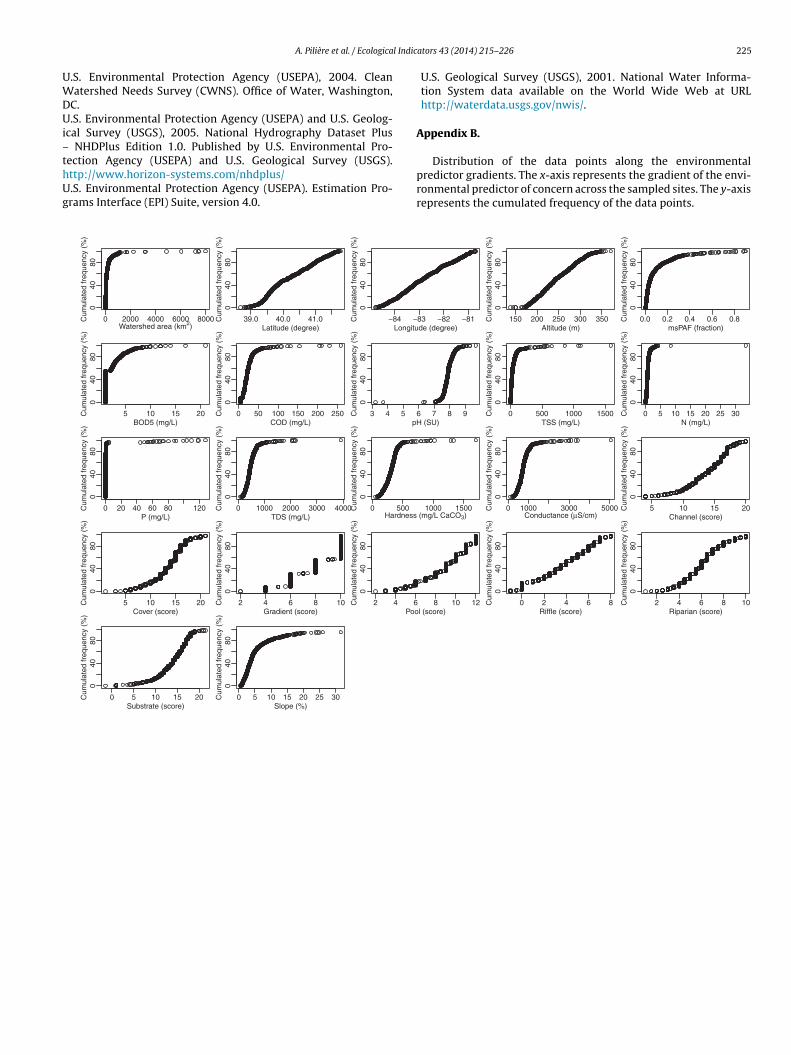
Appendix B.

Distribution of the data points along the environmentalpredictor gradients. The x-axis represents the gradient of the envi-ronmental predictor of concern across the sampled sites. The y-axisrepresents the cumulated frequency of the data points.

Page 12

2 l Indic

R

B

B

B

C

D

D

D

D

E

F

F

G

H

H

I

J

K

K

K

L

L

L

2007. A structured approach for developing indices of biotic integrity: threeexamples from streams and rivers in the western USA. Trans. Am. Fish. Soc. 136,718–735.

26 A. Pilière et al. / Ecologica

eferences

ae, M.J., Kwon, Y., Hwang, S.J., Chon, T.S., Yang, H.J., Kwak, I.S., Park, J.H., Ham,S.A., Park, Y.S., 2011. Relationships between three major assemblages and theirenvironmental factors in multiple spatial scales. Ann. Limnol. – Int. J. Limnol. 47,S91–S105.

edoya, D., Manolakos, E.S., Novotny, V., 2011. Characterization of biologicalresponses under different environmental conditions: a hierarchical modellingapproach. Ecol. Model. 222, 532–545.

ryce, S.A., Hughes, R.M., Kaufmann, P.R., 2002. Development of a bird integrityindex: using birds assemblages as indicators of riparian condition. Environ.Manage. 30, 294–310.

appo, M., De’ath, G., Boyle, S., Aumend, J., Olbrich, R., Hoedt, F., Perna, C., Brun-skill, G., 2005. Development of a robust classifier of freshwater residence inbarramundi (Lates calcarifer) life histories using elemental ratios in scales andboosted regression trees. Marine Freshw. Res. 56, 713–723.

e Zwart, D., Dyer, S.D., Posthuma, L., Hawkins, C.P., 2006. Predictive modelsattribute effects on fish assemblages to toxicity and habitat alteration. Ecol. Appl.16, 1295–1310.

e’ath, G., Fabricius, K.E., 2000. Classification and regression trees: a powerful yetsimple technique for ecological data analysis. Ecology 81, 3178–3192.

eKeyser, E.S., Kirby, D.R., Ell, M.J., 2003. An index of plant community integrity:development of the methodology for assessing prairie wetland plant communi-ties. Ecol. Indic. 3, 119–133.

olph, C.L., Huff, D.D., Chizinski, C.J., Vondracek, B., 2011. Implications of commu-nity concordance for assessing stream integrity at three nested spatial scales inMinnesota. USA. Freshw. Biol. 56, 1652–1669.

lith, J., Leathwick, J.R., Hastie, T., 2008. A working guide to boosted regression trees.J. Anim. Ecol. 77, 802–813.

riedman, J.H., 2001. Greedy function approximation: a gradient boosting machine.Ann. Stat. 29, 1189–1232.

riedman, J.H., Meulman, J.J., 2003. Multiple additive regression trees with applica-tion in epidemiology. Stat. Med. 22, 1365–1381.

renouillet, G., Brosse, S., Tudesque, L., Lek, S., Baraillé, Y., Loot, G., 2008. Concord-ance among stream assemblages and spatial autocorrelation along a fragmentedgradient. Divers. Distrib. 14, 592–603.

eino, J., 2010. Are indicator groups and cross-taxon congruence useful for predict-ing biodiversity in aquatic ecosystems? Ecol. Indic. 10, 112–117.

opkins, R.L., Whiles, M.R., 2011. The importance of land use/land cover data in fishand mussel conservation planning. Ann. Limnol. – Int. J. Limnol. 47, 199–209.

nfante, D.M., Allan, J.D., Linke, S., Norris, R.H., 2009. Relationship of fish and macroin-vertebrate assemblages to environmental factors: implications for communityconcordance. Hydrobiologia 623, 87–103.

oy, M.K., De’ath, R.G., 2004. Application of the Index of Biotic Integrity methodologyto New-Zealand freshwater fish communities. Environ. Manage. 34, 415–428.

arr, J.R., Kimberling, D.N., 2003. A terrestrial arthropod index of biological integrityfor shrub-steppe landscapes. Northwest Sci. 77, 202–213.

lemm, D.J., Blocksom, K.A., Fulk, F.A., Herlihy, A.T., Hughes, R.M., Kaufmann, P.R.,Peck, D.V., Stoddard, J.L., Thoeny, W.T., Griffith, M.B., Davis, W.S., 2003. Devel-opment and evaluation of a Macroinvertebrate Biotic Integrity Index (MBII)for regionally assessing Mid-Atlantic Highlands streams. Environ. Manage. 31,656–669.

nudby, A., Brenning, A., LeDrew, E., 2010. New approaches to modelling fish-habitatrelationships. Ecol. Modell. 221, 503–511.

arsen, S., Mancini, L., Pace, G., Scalici, M., Tancioni, L., 2012. Weak concordancebetween fish and macroinvertebrates in Mediterranean streams. PLoS ONE 7.(12).

eclere, J., Oberdorff, T., Belliard, J., Leprieur, F., 2011. A comparison of modeling

techiques to predict juvenile 0 + fish species occurrences in a large river system.Ecol. Inform. 6, 276–285.

eRoy Poff, N., 1997. Landscape filters and species traits: towards mechanisticunderstanding and prediction in stream ecology. J. North Am. Benthol. Soc. 16,391–409.

ators 43 (2014) 215–226

Manolakos, E., Virani, H., Novotny, V., 2007. Extracting knowledge on the linksbetween the water body stressors and biotic integrity. Water Res. 41,4041–4050.

Mantel, N., 1967. The detection of disease clustering and a generalized regressionapproach. Cancer Res. 27, 209–220.

Neff, M.R., Jackson, D.A., 2013. Regional-scale patterns in community concordance:testing the roles of historical biogeography versus contemporary abiotic con-trols in determining stream community composition. Can. J. Fish. Aquat. Sci. 70,1141–1150.

Neumann, G., Veeranagouda, Y., Karegoudar, T.B., Sahin, Ö., Mäusezahl, I., Kabelitz,N., Kappelmeyer, U., Heipieper, H.J., 2005. Cells of Pseudomonas putida andEnterobacter sp. adapt to toxic organic compounds by increasing their size.Extremophiles 9, 163–168.

Oksanen, J., Blanchet, G.F., Kindt, R., Legendre, P., Minchin, P.R., O’hara, R.B., Simpson,G.L., Solymos, P., Henry, M.H.H., Wagner, H., 2013. vegan: community ecologypackage. R package version 2.0-9.

Ohio EPA, 1987. Biological Criteria for the Protection of Aquatic Life: Volume II. UsersManual for Biological Field Assessment of Ohio Surface Waters. Division of WaterQuality Monitoring and Assessment, Surface Water Section, Colombus, OH.

Ohio EPA, 1989. Biological Criteria for the Protection of Aquatic Life: Volume III.Standardized Biological Field Sampling and Laboratory Methods for AssessingFish and Macroinvertebrate Communities. Division of Water Quality Monitoringand Assessment, Colombus, OH.

Ohio EPA, 2006. Methods for Assessing Habitat in Flowing Waters: Using theQualitative Habitat Evaluation Index (QHEI). OHIO EPA Technical BulletinEAS/2006/06/1.

Paavola, R., Muotka, T., Virtanen, R., Heino, J., Jackson, D., Maki-Petays, A., 2006.Spatial scale affects community concordance among fishes, benthic macroin-vertebrates, and bryophytes in streams. Ecol. Appl. 16, 368–379.

Padial, A.A., Declerck, S.A.J., De Meester, L., Bonecker, C.C., Lansac-Tôha, F.A.,Rodrigues, L.C., Takeda, A., Train, S., Velho, L.F.M., Bini, L.M., 2012. Evidenceagainst the use of surrogates for biomonitoring of Neotropical floodplains.Freshw. Biol. 57, 2411–2423.

Posthuma, L., Suter, G.W., Traas, T.P., 2002. Species Sensitivity Distributions in Eco-toxicology. Lewis Publishers, CRC Press, New York, NY.

Posthuma, L., De Zwart, D., 2006. Predicted effects of toxicant mixtures are confirmedby changes in fish species assemblages in Ohio, USA. Environ. Toxicol. Chem. 25,1094–1105.

Rooney, R.C., Bayley, S.E., 2012. Community congruence of plants, invertebrates andbirds in natural and constructed open-water wetlands: do we need to monitormultiple assemblages? Ecol. Indic. 20, 42–50.

Schipper, A.M., Lotterman, K., Geertsma, M., Leuven, R.S.E.W., Hendriks, A.J., 2010.Using datasets of different taxonomic detail to assess the influence of flood-plain characteristics on terrestrial arthropod assemblages. Biodivers. Conserv.19, 2087–2110.

Snelder, T., Barquín Ortiz, J., Booker, D., Lamouroux, N., Pella, H., Shankar, U., 2012.Can bottom-up procedures improve the performance of stream classifications?Aquat. Sci. 74, 45–59.

Waite, I.R., Kennen, J.G., May, J.T., Brown, L.R., Cuffney, T.F., Jones, K.A., Orlando, J.L.,2012. Comparison of stream invertebrate response models for bioassessmentmetrics. J. Am. Water Resour. Assoc. 48, 57–583.

Weigel, B.M., Lyons, J., Rasmussen, P.W., 2006. Fish assemblages and biotic integrityof a highly modified floodplain river, the Upper Mississipi, and a large, relativelyunimpacted tributary, the Lower Wisconsin. River Res. Appl. 22, 923–936.

Whittier, T.R., Hughes, R.M., Stoddard, J.L., Lomnicky, G.A., Peck, D.V., Herlihy, A.T.,

Williams, J.B., Poff, N.L., 2006. Informatics software for the ecologist’s toolbox: abasic example. Ecol. Inform. 1, 325–329.