COMPARING METHODS FOR MEASURING THE …oaktrust.library.tamu.edu/bitstream/handle/1969.1/ETD-TAMU-2009-12... · iii ABSTRACT Comparing Methods for Measuring the Volume of Sand Excavated

COMPARING METHODS FOR MEASURING THE VOLUME OF SAND EXCAVATED

BY A LABORATORY CUTTER SUCTION DREDGE USING AN INSTRUMENTED

HOPPER BARGE AND A LASER PROFILER

A Thesis

by

ARUN KUMAR MANIKANTAN

Submitted to the Office of Graduate Studies of Texas A&M University

in partial fulfillment of the requirements for the degree of

MASTER OF SCIENCE

December 2009

Major Subject: Ocean Engineering

COMPARING METHODS FOR MEASURING THE VOLUME OF SAND EXCAVATED

BY A LABORATORY CUTTER SUCTION DREDGE USING AN INSTRUMENTED

HOPPER BARGE AND A LASER PROFILER

A Thesis

by

ARUN KUMAR MANIKANTAN

Submitted to the Office of Graduate Studies of Texas A&M University

in partial fulfillment of the requirements for the degree of

MASTER OF SCIENCE

Approved by:

Co-Chairs of Committee, Robert E Randall David Brooks Committee Member, Billy Edge Head of Department, John Niedzwecki

December 2009

Major Subject: Ocean Engineering

iii

ABSTRACT

Comparing Methods for Measuring the Volume of Sand Excavated by a Laboratory

Cutter Suction Dredge Using an Instrumented Hopper Barge and a Laser Profiler.

(December 2009)

Arun Kumar Manikantan, B.E., Mumbai University

Co-Chairs of Advisory Committee: Dr. Robert Randall Dr. David Brooks

The research focuses on the various methods that could be used in the laboratory

to determine the values of production from a model cutter suction dredge. The values of

production obtained from different methods are compared to estimate the best value. The

tests were conducted in an attempt to pave the way to find spillage from the cutter

suction dredge. The development of these methods is useful for evaluating the sediment

spillage and residuals during dredging. The more accurate the values of production the

more accurate would be the values of spillage. For this purpose, the laboratory dredge

carriage and dredge/tow tank located at the Haynes Coastal Engineering Laboratory at

Texas A&M University is used. During the summer of 2007 and 2008, the laboratory

dredge carriage was used to dredge sand (d50 = 0.27 mm) in the sediment pit that is 7.6

m (25 feet) long, 3.7 m (12 feet) wide and 1.5 m (5 feet) deep. A laser profiler, a model

hopper barge attached with pressure gauges, a flowmeter and density gauge aid in

determining the production from the laboratory model of the cutter suction dredge were

used. The before and after bathymetry measurements using a laser profiling system are

used to determine the amount of sediment remaining after dredging. The hopper is

iv

instrumented with pressure gauges to measure the amount of sediment contained in the

hopper. The laboratory dredge system has a magnetic flowmeter and nuclear density

gauge that provide data to calculate the amount of sand delivered to the hopper. The

difference between the sand volume from the before and after bathymetry is the amount

of sand that is resuspended and subsequently resettles in the dredging area (residual) and

the sand that is not picked up by the dredge (spillage). Many issues in laboratory testing

were found during the course of testing and solutions were found. The production values

are compared with reasoning as to why the differences occur. The results demonstrate

the ability and difficulty of measuring the amount of material that is dredged and the

amount of spillage and residuals that occurs during dredging.

v

ACKNOWLEDGEMENTS

The author would like to express his deepest gratitude to Dr. Robert E. Randall

and Dr. David Brooks, the Co-Chairs for the Committee, for their support,

encouragement and direction, without which this would be next to impossible. The

author would also like to thank John Henriksen and Dustin Young for their invaluable

support during testing in the laboratory. The author is also grateful to Dr. Billy Edge for

serving as the committee member. The author would also like to thank Dr. Scott

Socolofsky for his timely and valuable support.

The author acknowledges the partial support for the research reported in this

paper through Dr. Joe Gailani of the US Army Engineering Research and Development

Center in Vicksburg, MS.

The author also wants to thank his parents for standing by him through the trials

and decisions of his educational career. 

vi

TABLE OF CONTENTS Page

ABSTRACT ...................................................................................................................... iii

ACKNOWLEDGEMENTS ............................................................................................... v

TABLE OF CONTENTS .................................................................................................. vi

LIST OF FIGURES......................................................................................................... viii

LIST OF TABLES ............................................................................................................. x

NOMENCLATURE .......................................................................................................... xi

CHAPTER I INTRODUCTION ........................................................................................ 1

1.1 Organization ........................................................................................................ 1 1.2 Introduction ......................................................................................................... 2

CHAPTER II LITERATURE REVIEW ............................................................................ 7

CHAPTER III SCALING LAWS .................................................................................... 14

3.1 Review ............................................................................................................... 14 3.2 Scaling of the model hydraulic dredge at Texas A&M. .................................... 17

CHAPTER IV EQUIPMENT DESCRIPTION ............................................................... 19

4.1 Laser profiler ..................................................................................................... 19 4.2 Model hopper barge ........................................................................................... 20 4.3 Pressure sensors ................................................................................................. 25 4.4 Data acquisition system ..................................................................................... 28 4.5 Data logger ........................................................................................................ 30 4.6 Magnetic flowmeter and nuclear density gauge ................................................ 31

CHAPTER V EXPERIMENTAL PROCEDURES ......................................................... 33

5.1 Procedures for experimental measurements ...................................................... 33 5.2 Calculation of time required .............................................................................. 38 5.3 Problems during set up and testing .................................................................... 39 5.4 Experimental methods ....................................................................................... 41

vii

Page

CHAPTER VI DATA ANALYSIS ................................................................................. 42

6.1 Method A: Using the laser profiler over the sediment pit. ................................ 42 6.2 Method B: Using the laser profiler over the sediments placed on the surface of the tow tank from the hopper. ........................................................... 44 6.3 Method C: Using pressure gauges attached to the model hopper barge. ........... 45 6.4 Method D: Using the flow meter and the density gauge on the carriage .......... 49

CHAPTER VII SUMMARY AND DISCUSSION OF RESULTS ................................. 52

7.1 Summary and discussions of results from all the tests. ..................................... 52

CHAPTER VIII CONCLUSIONS AND RECOMMENDATIONS ............................... 55

REFERENCES ................................................................................................................. 57

APPENDIX ...................................................................................................................... 59

VITA ................................................................................................................................ 63

viii

LIST OF FIGURES Page

Figure 1: A 3-D sketch of the dredge tow tank ................................................................ 3

Figure 2: Different views of carriage mounted on the rails of the tow tank with cutter seen in the bottom (right) ............................................................... 5

Figure 3: Profile laser (a) and the laser mounting system (b) ........................................ 19

Figure 4: User interface with the laser (c) ..................................................................... 20

Figure 5: Hopper barge resting on jacks (left) rubber tire act as fenders (right) ............. 22

Figure 6: Dimensions of the hopper barge. .................................................................... 23

Figure 7: Hopper attached to the carriage using a 10 feet long rod (left) and hopper doors closed and caulked before the dredging operation and a scale is shown that is used to measure the volume in the hopper (right). ................................................................................................. 24

Figure 8: General set up of the hopper ........................................................................... 24

Figure 9: The pressure sensor. ........................................................................................ 25

Figure 10: Example pressure calibration, depth vs voltage (Sensor1) ........................... 27

Figure 11: Example pressure sensor PVC tube (left) and pressure sensor at bottom of tube (right). .................................................................................... 27

Figure 12: Manual control system (left) next to PC automation system (right). ............. 29

Figure 13: The dredge carriage graphical user interface. ................................................. 29

Figure 14: Schematic of the data acquisition and control setup for the dredge/tow carriage. ....................................................................................... 30

Figure 15: Picture of the horizontal position laser mounted on the dredge/tow carriage ........................................................................................................... 30

Figure 16: Picture of the data logger. ............................................................................... 31

Figure 17: Two way valve, with the nuclear density gage and flowmeter attached to it. .................................................................................................. 32 

ix

Page

Figure 18: General set up of the experiment. ................................................................... 33

Figure 19: Schematic of the volume of sand removed when moving from A to B (left) motion of the cutter suction dredge (right). ....................................... 35

Figure 20: Blown up view of cutter in the sediment pit .................................................. 37

Figure 21: The filter being placed between the hopper and sediment pit (left) the bottom of the tow tank after the filter is removed (right) ......................... 40

Figure 22: Laser Profiler on the frame, hanging from the top of the tow tank (left) hose attached to the hopper barge (right) ............................................ 41

Figure 23: A profile of the sediment pit (left), generated by MATLAB; the eight cuts can be distinctly seen. (Test 7) ...................................................... 42

Figure 24: A profile of the dropped sediments generated by MATLAB; the eight cuts can be distinctly seen. .................................................................... 44

Figure 25: The two way valve on the carriage (left) schematic of model hopper (right). ............................................................................................. 46

Figure 26: Graph showing the increase in weight of the hopper as draft (h) changes. .......................................................................................................... 47

Figure 27: Graph showing the change in volume of the hopper as Im changes............... 48

Figure 28: An example of the production plot while discharging slurry into hopper barge during dredging with model cutter suction dredge. ................. 51 

x

LIST OF TABLES Page

Table 1: Specifications of the model dredge carriage. ..................................................... 4

Table 2: Parameters of the model dredge at the facility, (scale of 1:6) ...........................18

Table 3: Specifications of the pressure sensor. .............................................................. 26

Table 4: The test matrix for the 7 day testing period ..................................................... 34

Table 5: The expected time required for testing............................................................. 38

Table 6: Volume of sand removed using the laser profiler over the pit. ........................ 43

Table 7: Volume of sand removed using the laser profiler over the pile. ...................... 45

Table 8: Example calculation of dredged sand volume for pressure sensor #1 ............. 49

Table 9: Values of production in Cu Yd for different values of SG ................................ 51

Table 10: Summary of results from all the methods ........................................................ 52

xi

NOMENCLATURE

= Cutterhead angular velocity....rad/s

= Diameter of cutter head....m (in)

= Average suction pipe flow velocity....m/s (ft/s)

C = Concentration factor..

cutter

cutter

suction

v

D

U

ω

..-

= Specific Gravity of mixture (sand and water)....-

= Specific Gravity of fluid (water)....-

= Specific Gravity of solids (sa nd)....-

= Velocit

m

f

velocity

s

SG

SG

H

SG

3 3

y head....m (ft)

= Volumetric flowrate through suction /

discharge pipe....m /s (ft /s)

= Cutterhead swing velocity....m/s (ft/min)

= Gravitatio

nal accelerat

ion c

suction

swing

Q

V

g 2 2onstant....m/s (ft/s )

= Settling velocity....mm/s (ft/s)

= Internal height of the hopper....mm (in)

= Draft of the hopper....mm (in)

= Total weight of the h

settling

m

t

V

I

h

W opper....kg (lb)

= Weight of the empty hopper....kg (lb)

= Weight of the slurry in the hopper....kg (lb)

= Specific Gravity of water....-

= Displaced volume of

e

i

w

d

W

W

V

γ

the hopper....cu.m (cu.yd)

= Volume of slurry in the hopper....cu.m (cu.yd)

= Volume of the cuboid....cu.m (cu.yd)

= Volume of the frustrum of a pyramid....cu.m (cu.yd)

s

c

p

m

V

V

V

I = Height of the frustrum of a pyramid....mm (in)

= Height of the cuboid....mm (in)

p

mcI    

1

CHAPTER I

INTRODUCTION

1.1 Organization

The Haynes Coastal Engineering Laboratory hosts a Dredge Tow Tank where the

experiments were conducted for measuring the production of the spillage of sand

resulting from a model cutter suction dredge. Different methods were used so as to

calculate the production resulting from the model cutter suction dredge. The thesis starts

with introducing the facility at Texas A&M University where the experiments were

conducted. This section is followed by a literature review, which encompasses the

previous research and discusses the results. The different dredging parameters and

scaling laws applicable to the experiment are discussed in Chapter III. The various

equipments available at the laboratory and their usability are discussed in chapter IV.

Chapter V describes the experimental setup procedure and chapter VI discusses the

different methods of calculating the dredge production, the instrumentation used on the

hopper barge and the laser profiler. Finally the thesis describes the experimental data and

discusses the results from all four different types of dredge production calculations used

in the experiment.

___________ This thesis follows the style of Journal of Dredging Engineering.

2

1.2 Introduction

The quantification of the amount of material dredged has always been very

difficult. The resuspension, spillage and turbidity are a few of the many reasons why the

quantification becomes difficult. In this experiment, various types of attempts have been

made to quantify the amount of sand dredged, and the quantities are compared which

helps to determine the approximate quantity of sand removed, using a cutter suction

dredge.

The dredge/tow tank facility at the Haynes Coastal Engineering Laboratory

(Figure 1) at Texas A&M University has been utilized for this purpose. The installation

of the basic dredge tow carriage in Haynes Laboratory was completed in 2005. Several

model tests have been conducted and finished in this laboratory dredge/tow tank,

including: modeling of simulated oil spills, scouring around bridge structures, modeling

forces on strakes, resuspension of dredged material by cutter suction dredge, effect of

debris on dredging production, measurement of cutter force, operation of bed levelers

and others. The laboratory houses a state-of-the- art model cutter suction dredge. The

model dredge comprises of a carriage, ladder, and cradle. The entire assembly is

mounted rails attached to the tow tank walls. The model cutter suction dredge, as shown

in Figure 2, is supported by a carriage that runs on the rails of a 45.72 m (150 ft) long,

3.657m (12 ft) wide, and 3.353mt (11 ft) deep dredge/tow flume. The 0.3 m (12 in)

cutter is mounted on an articulating ladder, attached to a vertical ladder that runs

transverse to the carriage. The upward and the downward movement of the cutter are

facilitated using the vertical and articulating ladder.

3

The towing carriage traverses on the steel flume rails using polyurethane rimmed steel

wheels along the top of the tow tank side walls, while the cradle moves in a direction

perpendicular to the movement of the carriage. The vertical ladder is on the upper side

while the articulating ladder is in the lower side of the carriage. These allow both

vertical translation and an adjustable angle of the lower ladder between 0 and 50 degrees

with the horizontal, respectively. The cutter is attached to the end of the articulating

ladder and the suction inlet is located directly behind the cutter. The dredge/tow tank

also has an additional 7.62 m (25 ft) long by 1.524 m (5 ft) deep sediment pit. The

sediment pit is covered when the experiments are not using the sediment pit. A

maximum of 2.233 L/s (35,000 GPM) of water can be pumped through the flume using

the four axial flow pumps. For a dredging production test, the tow tank is filled with up

to 6 feet of water. The specifications of the carriage are tabulated in Table 1.

Figure 1: A 3-D sketch of the dredge tow tank.

4

Table 1: Specifications of the model dredge carriage

Category Characteristic

Maximum Carriage Speed 2 m/s (6.6 feet/s)

Total Dredge/Tow Carriage Weight 4545 kg (10,000 lb)

Cradle Weight 1364 kg (3,000 lb)

Ladder Weight 909 kg (2,000 lb)

Carriage Power Two 3.8 kW (5 hp) motors

Cutter Power 7.5 kW (10 hp)

Pump Power 14.9 kW (20 hp)

Side to Side Cradle Motor Power 1.1 kW (1.5 hp)

Vertical Ladder Motor Power 1.1 kW (1.5 hp)

Articulating Ladder Position Motor Power 0.5 kW (0.8 hp)

Dredge Pump Flow Rate Maximum 1893 LPM (500 GPM)

Dredge Pump Size 10.4 cm ( 4 in), suction; 7.62 cm (3 in), discharge

Control System Ethernet PLC Automated and manual operation

Data Acquisition Real-time display and data storage

Swing Travel 1.6 m (5.3 feet) on either side of flume centerline

Ladder Angle 0 to 50 degrees from horizontal

5

Figure 2: Different views of carriage mounted on the rails of the tow tank with cutter seen in the bottom (right).

Apart from the testing of production from the model cutter, the facility is used for

efficient testing of different drag heads, suction heads, cutterheads, and hopper

placement of dredged material. Real time experiments like studies on the effects of bed

leveling on model turtles or of mangrove roots on production have been simulated in the

dredge/tow tank.

A sand/water separation system was also installed on the Dredge/Tow Carriage.

The Tri-Flo model 300 sand/water separation unit is designed to have a storage tank with

a capacity of 1136 liters (300 gallons). The system is able to handle separation of solids

and water at a pumping load of up to 454 liters per minute (120 gallons per minute). If

allowed to pump back into the tank, the discharge pump can also act as a “bottom

agitator”. A 1136 liter (300 gallon) tank, a scalping shaker, a mud cleaner consisting of

two 10.2 cm (4 in) hydro cyclones mounted on a drying shaker, a mud gun, two 5.1 cm

by 7.6 cm (2 in by 3 in) closed coupled centrifugal pumps, and solid slides to deliver

6

solids to holding bins comprise the sand/water separation system. It is 157.5 cm (62 in)

wide, 226 cm (89 in) long, and 233.7 cm (92 in) in height. The total empty weight is

1225 kg (2700 lb) and the total full weight is 2858 kg (6300 lb).  

A magnetic flow meter and a nuclear density gauge are additional instruments on

the carriage, and they facilitate measuring the instantaneous flow and specific gravities

of the slurry, respectively. The laboratory also has a model hopper barge that is used to

study the production. The hopper is instrumented with pressure gauges to study the

production of sand from the model cutter suction dredge. This process is accomplished

using draft measurements. The laboratory also has a Laser profiler that is used to

calculate the volume of sediments dredged by knowing the before and after bathymetry

of the sediment pit.

7

CHAPTER II

LITERATURE REVIEW

Tests were conducted using a cutter suction dredge on the Corpus Christi Ship

Channel on a clay sediment bed by Huston and Huston (1976). They concluded that the

level of turbidity increases in the immediate vicinity of the cutter and the increased

levels of turbidity (variable) are due to an increase in the suspension of fine grained

material created from cutter turbulence. The variability of the turbidity is inconsistent in

the immediate vicinity of the cutter, possibly due to cutter generated turbulence which

increases the turbidity at higher rpm. This inconsistency could also be influenced by the

variability of the material being dredged and/or the suction velocity. They also

concluded that very little turbidity created by the cutter rises into the water column (9 to

12 m deep). This is proven by the fact that no substantial visible surface turbidity was

observed.

Herbich and Brahme (1983), conducted studies on conventional and

unconventional dredges, their dredging techniques, turbidity generation and ways to

improve these dredges so as to reduce the environmental impact. Turbidity is also one of

the results of the sediments that have not been picked up by the dredge (resuspension).

The authors have discussed turbidity and its effects (physical, chemical and biological)

on the environment, turbidity generation, turbidity generation potential of sediments and

prediction of turbidity due to different dredges. Finally, the authors have suggested

methods to reduce the turbidity in various dredges using different techniques. According

to the authors, given a set of conditions, the dredging equipment, skill of the operator

8

and the type of dredge create different levels of turbidity. The cutterhead dredge is the

most commonly used dredge in the United States, and the typical solid contents of the

sediments pumped is 10 to 20 percent by volume, for a pipeline size that varies from 15

cm to 112 cm (6 in to 44 in). Most of the resuspension for the cutter suction dredge

occurs in the vicinity of the cutter. The rate of cutter rotation, the vertical thickness of

the dredge cut, the velocity (horizontal) of the cutter moving across the cut, and the skill

of operator greatly influence the amount of resuspension. Field data for sediment

resuspension was collected under low current conditions, and the concentrations in the

vicinity of the cutter (3m) are highly variable (as much as 10s of grams per liter). These

concentrations are observed to decrease exponentially towards the surface and are in the

order of a few hundred milligrams per liter at distances of a few hundred meters from a

cutter. An improperly designed cutter creates greater turbulence which in turn affects

resuspension. Excessive cutter rotation speed also tends to throw the sediments away

from the cutter.

Resuspension from a cutter suction dredge is a process wherein some amount of

the dredged material is suspended back into the vicinity of dredging. Schroeder (2009),

discusses, the 3Rs of dredging namely Resuspension, Release and Residuals.

Resuspension, is defined, as the dislodgement and dispersal of sediments into the water

column where finer sediment particles and floccus are subject to transport and dispersion

by currents, and residuals are defined as the sediments dislodged but not removed by

dredging, which falls back (spillage), or settles in or near dredging foot print and forms a

new sediment layer. Resuspension is often characterized by dispersion of sediment

9

(turbidity). Herbich (2000) discusses the resuspension of sediments during the dredging

operation and indicates that the factors causing dispersion depends upon the type of

dredge, method of dredging and the environmental conditions. But the degree of

resuspension is largely governed by the size of sediment particles being dredged.

Extremely fine particles have a higher tendency to go into suspension as they are

supported by buoyancy. He also talks about the composition of solids and water mixture

which gives us an approach to measure the volume of solids in the hopper. The

composition of the mixture is the ratio of the volume of solids to the volume of the

mixture. Concentration by volume of solids in a mixture, Cv, is the ratio of volume of

solids to volume of mixture and is expressed as

C SG SGSG SG 1

where, SGm SGs and SGw are the specific gravities of the mixture, solids and water

respectively.

Glover and Randall (2004), based on previous model studies, develop grounds

for scaling the model dredge operating parameters at the Texas A&M University’s Reta

and Bill Haynes ’46 Coastal Engineering Laboratory. They have demonstrated how the

similitude criteria can be used in an actual model dredge study. Performance of a model

dredge depends on the extent to which the kinematic, dynamic and geometric similarities

are attained between the model and the prototype. Hypothetical model studies on a cutter

suction dredge were conducted to show how effectively the similitude criteria could be

used. For this purpose, numerous model studies were reviewed, such as model dredge

10

studies, flow visualization studies, model cutterhead studies, flow field studies and

sediment pick up behavior, cavitations and cutterhead dynamics. The scaling laws for

modeling the hydraulic dredging operation were reviewed and suggest that the best

method to model the dredge in a laboratory facility is based on the sediment pick up

behavior. It also suggests that the velocity fields must all be scaled in accordance with

the geometric scale ratio and normalized to the sediment settling velocity. Experiments

are conducted on the model dredge facility to determine the effect of swing speeds on

the production for a given cutterhead design, and the swing speeds are varied and all

other parameters are kept constant. It was found that the higher swing speeds result in

lower production because of spillage. Also, some of the recorded quantities, such as the

cutterhead forces, cutterhead power and pump characteristics like the pump power, head

and slurry specific gravity, are not easily scalable. However, the effect of the swing

speed on these parameters can be observed. One of the limitations observed here was

that the dynamic similarity cannot be attained simultaneously with the hydraulic

similarity. This would mean if the cutterhead speeds and the swing speeds are increased,

so as to obtain similarity with respect to cavitation, then, the similarity due to sediment

pick up behavior would have to be compromised.

Burger, Vlasbom and Talmon (2005) conducted experiments at the Delft

University to improve the cutterhead design so as to minimize the spillage, which would

help increase production. The efficiency of the cutterhead varies based on the type of

bed being dredged. Experiments are conducted to observe the amount of spillage for

various speeds of the cutterhead and solutions are recommended based on the

11

observations. The experiment consists of a prototype whose size compared to the

working model is a ratio of 1:8 with the cutterhead shaft at an angle of 45 degrees. The

experiment focuses on mixture formation processes while dredging a rock/hard clay bed.

A prototype bed that would replicate similar effects while dredging rock/hard clay bed is

prepared by weakly cemented gravel of density 2650 Kg/m3.The results show that

production increases with an increase in rotational speed but decreases with further

increase in speed. The reason for the first phenomena is observed as low rotational speed

leads to the accumulation of particles at the lowest point of the cutterhead due to the

dominance of gravitational force. The second phenomena where there is a reduction of

production with higher rotational speed is explained as an increase in centrifugal force,

which leads to particles being thrown away from the cutter. This also necessitates an

increase in pump capacity to capture the remaining particles by maintaining a constant

suction flow. With the above results, a graph for optimum cutterhead speed and optimum

pump capacity for a given cutterhead dimension is drafted. The article further concludes

that low efficiency of the cutterheads can be improved by redefining the pump capacity

and cutterhead dimensions based on the graph.

Palermo and Randall (1990) investigated the overflow characteristics of a

hopper, to load the hoppers economically. The resource agencies have put restrictions on

the overflow. However, the need for restriction or data that technically supports

overflow need to be found. Palermo and Randall (1989) recommended the development

of techniques that would predict the potential load gain in hoppers and scows. This

knowledge would provide guidance on when the overflow could potentially achieve load

12

gains. Also, they recommend the development of equipment to aid in the retention of

material in the hopper and scows. Miller, Palemro, and Groff (2001) studied the hopper

overflow for the Delaware River, wherein they have sampled the hopper inflow to

analyze the grain size distribution, particle size distribution of fines and chemical

concentrations. Similar analysis in the experiment could render a basis for the estimate

of the percentage of sand removed during dredging. Hopper contents are also sampled

here so as to know the concentrations of suspended solids. Studies of this nature

necessitate the need to know the amount of sediments dredged into the hopper.

Fortino (1966) describes the pneumatic and electrical methods to measure the

flow of the dredged materials from the pump. This method can be used to measure the

sediments in the hopper Over the years, many attempts to measure the amount of

sediments in the hopper have been made. Armstong and Grant (1977) designed a float

that was used to measure the sediment in a hopper to determine the pay load of a trailer

suction dredge. This measurement device is mechanical and gives a continuous record of

the dredged sediments in the hopper, based on the relative density for which it is set.

Rokosch, Van Vechgel and Van der Veen (1986) investigated the challenges to measure

the optimum load for mixed loads. Mixed load is a combination of settled and suspended

materials. They examined the ‘Displacement and Pressure’ based measurements and

found that the total load and suspended material in a mixed load can be separately

determined. This result can be used to determine the continuation of loading the material

in the hopper. A different approach was used by Meyer et al (1986) to measure the

sediments in the hopper. They stated that dredge displacement is insufficient to

13

measure optimum load for fine sediments as it fails to determine the distribution of load

from fore to aft of the hopper. They suggested the use of a gamma emitting probe that

helps to show material build up in the hopper as a function of time for fine sediments. It

also determines the distribution of load throughout the hopper. However, this method is

inadequate to measure the load for fine grained sediments, but it is adequate enough for

sandy sediments.

14

CHAPTER III

SCALING LAWS

3.1 Review

This chapter describes the scaling relationships between operating parameters for

the hydraulic dredge model studies. The degree of geometric, kinematic and dynamic

similarity determines the usefulness of the hydraulic model dredge. Glover (2002)

studied the modeling of a model dredge facility in a laboratory. Even though the process

of modeling is extremely difficult, researchers have tried to isolate the different

processes. Evaluation of the scale effects is determined by different model scales.

Sometimes the models are as close as possible to the prototype, where in the errors due

to scale effects are minimized. Scales of 1:10 or sometimes 1:6 are better for model

dredging studies. According to Glover and Randall (2004), based on previous model

hydraulic dredge studies, the scaling laws can be divided into the following three

categories:

i. Similarity based on the sediment pick up behavior

ii. Similarity based on the cavitation during the cutting process

iii. Similarity based on the Froude or Reynolds number

It is stated that all of the above criteria cannot be satisfied by using one set of

operating parameters. It is well proven by researchers, such as Slotta (1968), J oanknecht

(1976), Brahme (1983), Herbich and Herbich (1983), and Burger (1997) that the similarity

based on the sediment pick up behavior is the most effective one. To model the

15

hydraulic dredge based on the Froude or Reynolds number or on the cavitation during

the cutting process requires parameters such as higher speeds (cavitation) and excessive

cutting swing speeds. These parameters are not realistically attainable in the laboratory.

Slotta (1968) developed relationships by dimensionless analysis of the cutterhead

and suction pipe parameters. The following equations were found to accurately correlate

the data for volumetric flow rate, suction velocity and cutterhead speeds.

model prototype

cutter cutter cutter cutter

suction suction

D DU U

ω ω⎡ ⎤ ⎡ ⎤⎢ ⎥ ⎢ ⎥⎢ ⎥ ⎢ ⎥⎣ ⎦ ⎣ ⎦

=                                                   (2) 

( ) ( )3 34 4

model prototype

cutter cuttersuction suction

velocity velocity

Q Q

H H

ω ω⎡ ⎤ ⎡ ⎤⎢ ⎥ ⎢ ⎥⎢ ⎥ ⎢ ⎥⎢ ⎥ ⎢ ⎥⎢ ⎥ ⎢ ⎥⎣ ⎦ ⎣ ⎦

=                                           (3)  

 In another instance, Joanknecht (1976) uses scaling of cutter forces without

taking sediment pick up, production or cavitations into consideration to model the

prototype. The equations are:

model prototypecutter cutter

swing swing

g gD DV V⎡ ⎤ ⎡ ⎤

⎢ ⎥ ⎢ ⎥⎢ ⎥ ⎢ ⎥⎣ ⎦ ⎣ ⎦

=                                                                    (4)

model prototype

swing swingcutter cutter

V Vg g

N N⎡ ⎤ ⎡ ⎤⎢ ⎥ ⎢ ⎥⎢ ⎥ ⎢ ⎥⎣ ⎦ ⎣ ⎦

= (5) 

16

Glover and Randall (2004) also states that for a similarity between the scale

model and prototype to be attained, with respect to the sediment pick up behavior, the

velocity fields must be normalized to the sediment settling velocity after the velocity

fields are all scaled with the geometric scale ratio. Herbich and Brahme (1986) showed

that the velocity field scaling factor depended on volumetric flow rate as opposed to

velocity at the suction inlet as Slotta (1968) stated. Thus, the equation (2) was rewritten

as equation (6).  

model prototype

cutter cutter cutter cutter

settling settling

N ND DV V

⎡ ⎤ ⎡ ⎤⎢ ⎥ ⎢ ⎥⎢ ⎥ ⎢ ⎥⎢ ⎥ ⎢ ⎥⎣ ⎦ ⎣ ⎦

= (6)

Equation (6) is derived from the fact that a velocity field relative to the

cutterhead is created which interacts with the velocity fields created by the cutterhead

rotation and suction. The velocity field relative to the cutterhead is created due to the

swing speed of the cutterhead. Herbich and Brahme (1983) arrive at Equation 7, based

on studies, with dimensionless velocity field plots, which show that the velocity field

was more a function of the volumetric flowrate through the suction pipe. When the

settling velocity of the model and the speed of the cutterhead are known, the model flow

rate, swing speed and cutterhead rotation speed can be scaled based on equations (6), (7),

and (8).

( ) ( )2 2

model prototype

suction suction

cutter cuttersettling settling

Q QD V D V

⎡ ⎤ ⎡ ⎤⎢ ⎥ ⎢ ⎥⎢ ⎥ ⎢ ⎥⎢ ⎥ ⎢ ⎥⎣ ⎦ ⎣ ⎦

= (7)

17

model prototype

swing swing

settling settlingVV V

V⎡ ⎤ ⎡ ⎤⎢ ⎥ ⎢ ⎥⎢ ⎥ ⎢ ⎥⎣ ⎦ ⎣ ⎦

=                                                                                 (8)

Glover and Randall (2004), also state that the dynamic scaling of cutting forces

depend upon bed sediment compactness ratio, dynamic scaling of particle settling

velocities, void ratio, material density and cohesive / adhesive properties. However,

finding these parameters is a major challenge for researches attempting to calculate

sediment scaling.

3.2 Scaling of the Model Hydraulic Dredge at Texas A&M

The model cutter suction dredge at Texas A&M, where the experiments were

conducted, is modeled using the similitude criteria. Here, again, the sediment pick up

behavior is the basis of the scale laws, while the median grain size and the geometric

scale ratio decide the basis of operating parameters. A chart for selecting the model

dredge operating parameters is used for the selection of geometric scale. The resulting

operating parameters for the model are known if the prototype grain size is known. The

data used to plot the charts are calculated from the equations (6), (7), (8). A deviation

from the model grain size would necessitate the calculation of the model to a prototype

velocity scale based on relative settling velocities.

Table 2 shows the parameters of the prototype and the model with a scale of 1:6. 

18

Table 2: Parameters of the model dredge at the facility, (scale of 1:6)

Parameter Prototype Model Scale

Cutter Diameter 183cm (72in) 30.5cm (12in) 1:6

Water Depth 12.2m (40feet) 3.35m (11feet) Not scaled

Depth of Cut 91.4cm (36in) 15.2cm (6in) 1:6

Sediment Diameter 0.2mm 0.1mm Not scaled

Settling Velocity 22.7mm/s 8.8mm/s 0.388

Suction Diameter 61cm (24in) 7.62cm (3in) 1:8

Suction Flow rate 113,562LPM

(30,000GPM) 1223LPM (323GPM) 0.011

Cutter RPM 40 124 3.104

Max Swing Speed 50cm/s (20in/s) 19.7cm/s (7.76in/s) 0.388

The model dredge is designed on the basis of the hydraulic similarity between the

model and the prototype. This ensures kinematic similarity, which means, according to

scaling laws, the model dredge will geometrically pick up the same amount of material

as that of the prototype. Cavitation coefficients and cutting forces restrict the dynamic

similarity of the dredge.

19

CHAPTER IV

EQUIPMENT DESCRIPTION

4.1 Laser Profiler

An optically safe laser mounted on an aluminum frame is used to aid the

quantification of sediments removed during the dredging process. The laser translates in

the longitudinal (x) and lateral (y) horizontal directions, as it takes the depth readings in

the “z” direction. The laser measures a distance (depth, z) of 200 to 1000 mm with a

resolution of 0.02 - 0.5 mm with an error of +/-2 mm. The laser, in this case, is

programmed to take depth readings at every 5 mm and 20 mm x and y increments,

respectively. The maximum reach of the laser is an area of 5000 mm by 2500 mm.

Pictures of the laser on the aluminum frame are shown in Figure 3.

    (a)                                                                                       (b) 

Figure 3: Profile laser (a), the laser mounting system (b).

20

(c) 

Figure 4: Laser Profiler User interface with the laser (c).  

The laser continuously measures the depth and stores the readings in the form of

both a Notepad (.dat) and a text file (.txt). The interface between the user and the Laser

profiler is as shown in Error! Reference source not found.. The parameters, like the X

and Y increments, absolute positions and the relative positions of the laser head, can be

adjusted using the interface. The .dat file is an input to a MATLAB code that is used to

calculate the volume of the dredged sediment.

4.2 Model Hopper Barge

The model hopper barge is constructed with a 3/32in thick steel plate. The outer

dimensions of the hopper are 73.15 x 40.23 x 18.28m (240 x 132 x 68in), while the

internal volume is 562 ft3 (20.8 yd3). The complete weight of the hopper is 6416 lbs.

21

This is calculated using the draft measurements from the sensors attached to the four

sides of the hopper.

The hopper rests on top of the tow tank on 3 I-beams when experiments are not

being conducted. The hopper is maneuvered by the laboratory’s electric overhead crane,

which has a capacity of 6000 lbs. The hopper doors, which weigh approximately 1000

lbs, are dissembled from the hopper before it is lifted by the crane in order to restrict the

total weight to the 6000 lb crane capacity. The hopper rests on four jacks inside the tow

tank when the tank is not filled with water. Once the hopper is in the tank, the doors are

then fitted. The hopper has two winches mounted on the top of the barge with their

cables and chains attached to the doors at the bow and stern; these winches are used for

the opening and closing of the hopper doors. Rubber tires (Figure 5) are attached on all

four sides of the hopper and act as fenders to prevent the hopper from hitting the walls of

the tank. When the hopper floats in water, the doors do not open completely due to the

buoyancy force of the water acting on the doors. Lead blocks are attached to the doors to

overcome this problem.

22

Figure 5: Hopper barge resting on jacks (left) rubber tires act as fenders (right).

Pressure sensors are housed in water tight PVC pipes and are attached on all four

sides of the hopper. The pressure sensors are used to measure the amount of slurry

collected in the hopper during dredging. A data acquisition system (DAS) captures

pressure variation every second and converts it into an electrical signal. Measuring tapes

attached to the PVC pipes help in knowing the draft of the hopper when empty and full.

The draft of the empty hopper is 17.8cm (7in), and thus the weight of the hopper is

calculated to be 2910kg (6416lb). A linear scale is drawn in the internal volume so as to

give a fair idea of the slurry height in the hopper. This scale is also used to calculate the

volume of sand in the hopper. Before the dredge/tow tank is filled with water, the hopper

doors are completely closed and caulked. The hopper is attached to the carriage by a

3.05m (10ft) long rod and moves in the same direction as the carriage, maintaining a

constant gap between the carriage and the hopper. Once the dredging operation starts,

the slurry is pumped into the hopper. A provision for overflow is provided to drain the

excessive water. After dredging is completed, the carriage and the hopper are moved to

23

the extreme end of the tow tank, away from the pit where the hopper doors are opened to

release the sediment from the hopper. Throughout the dredging operation, the data from

the pressure sensors are continuously recorded and analyzed to acquire the weight of the

sediments in the hopper. The schematic of the hopper is as shown in Figure 6. The

hopper is attached to the carriage by means of a 10ft long tie-rod, maintaining a constant

gap as the carriage moves backward and forward (Figure 7). The attachments to the

hopper are shown in Figure 8.

Figure 6: Dimensions of the hopper barge.

4

Plan View B

L

B

View A-A

AA

C

View B-B

LC240

60

192

44 44132

24 192 24240

8424 24

All dimensions are in inches

24

Figure 7: Hopper attached to the carriage using a 10 feet long rod (left) and hopper doors closed and caulked before the dredging operation and a scale is shown that is

used to measure the volume in the hopper (right).

Figure 8: General set up of the hopper.  

25

4.3 Pressure Sensors

Four pressure sensors (Figure 9) were used in the experiment, each sensor

attached to a different side of the hopper. The pressure sensors used are the Omegadyne

- PX309 015G5V, which are stainless steel high performance pressure transducers.

Ruggedness, solid state design, high stability, and low drift are the characteristics of

these pressure transducers. Figure 9 shows the pressure sensor. These sensors have a

gauge pressure range of 1-15psi and have an electrical cable output. The other end of the

cable is connected to a data logger, which is capable of recording continuous change in

pressure. Table 3 shows the specifications of the Omegadyne - PX309 015G5V sensor.

Figure 9: The pressure sensor.  

26

Table 3: Specifications of the pressure sensor  

Category Characteristic

Excitation: 9 to 30 Vdc (<10 mA) (reverse polarity and overvoltage protected)

Output: 0 to 5 Vdc

Accuracy: ±0.25% includes linearity, hysteresis and repeatability

Operating Temperature: -40 to 85ºC (-40 to 185ºF)

Weight: 155 g (5.4 oz) max

Prior to testing, each of these pressure sensors is housed in water tight PVC pipes

and is calibrated at different depths of water. The PVC pipes were held together and

lowered until the probes just touched the water surface, and the data for the depth of zero

inches was recorded for a period of 30 s. Similar readings were recorded at depths of 5.1

cm, 10.2 cm and so on up to 96.5 cm (i.e. 2 in, 4 in and so on up to 38 in). The pressure

sensor records one signal every second, and thus approximately 30 readings for each

depth were obtained. The calibration curves show the sensors are linear as demonstrated

in Figure 10. These calibrated sensors housed within the PVC pipes are attached to all

four sides of the hopper as shown in Figure 11.

27

Figure 10: Example pressure calibration, depth vs. voltage (Sensor1).

Figure 11: Example pressure sensor PVC tube (left) and pressure sensor at bottom of tube (right).

The four sensors are attached using clamps at the center of all four sides of the

hopper. As the hopper is filled during the dredging operation, the water pressure on the

0

100

200

300

400

500

600

700

800

900

0 5 10 15 20 25 30 35 40

Volta

ge

Draft (in) of the Hopper

Pressure Calibration Curve

28

sensors increases or decreases as the weight on the floating hopper increases or

decreases respectively. Data from each pressure sensor are identified, and the readings

are continuously recorded, using the data logger every second as the hopper is filled.

These data are compared to the calibrated data to determine the draft of the hopper and

the weight of the slurry in the hopper.

4.4 Data Acquisition System

An interactive graphical interface on a personal computer (PC) is used to access a

manual operating station and essential drives to operate Dredge/Tow Carriage. The

operational data from the gauges is recorded in the PC. The last feature includes

programmable dredging simulations replicated through the Graphical User Interface

(GUI). Figure 12, below, illustrates a manual operating station and a dredge automated

PC.

Figure 13 shows diagrammatic presentation of data acquisition system and

dredge carriage operating components, while Figure 14 illustrates the schematic of the

DAS and control setup for the dredge/tow carriage. The carriage movements can be

controlled through GUI or manual controls from the operation station. In both cases, the

data is exchanged between hubs and servo/vector programmable logic computers (PLC).

A servo PLC is used for controlling tower, cradle, and ladder movements, and a vector

PLC is used to control carriage, cutter and pump movements. A laser accompanied with

vector PLC determines the horizontal position of the carriage along the tank as shown in

Figure 15.

29

Figure 12: Manual control system (left) next to PC automation system (right).  

Figure 13: The dredge carriage graphical user interface.

30

Figure 14: Schematic of the data acquisition and control setup for the dredge/tow carriage.

Figure 15: Picture of the horizontal position laser mounted on the dredge/tow carriage.  

4.5 Data Logger

The data logger used is a Campbell Scientific make CR10X-series. It is compact and

has a modular line of data loggers with a measurement and control module, external

power supply, and keyboard display. Figure 16 shows a picture of the data logger.

31

Figure 16: Picture of the data logger.  

4.6 Magnetic Flowmeter and Nuclear Density Gauge

The flowmeter is a Krohne IFC 090 K magnetic flowmeter that is calibrated in

both stagnant and moving water and is mounted inline in a vertical section of the 7.6

cm (3 in) discharge line. Output for the flowmeter is a 4-20 mA signal. In order to

monitor the slurry or water flow, the output data from the flowmeter is sent to the data

acquisition system.

The nuclear density gauge is located below the flowmeter, and it is clamped onto

the 7.6 cm (3 in) vertical discharge pipe. The nuclear density gauge installed on the

Dredge/ Tow Carriage is an Ohmart Vega DSG radiation-based density measurement

system that renders outputs in the range of 4 to 20 mA signal. The gamma-based density

32

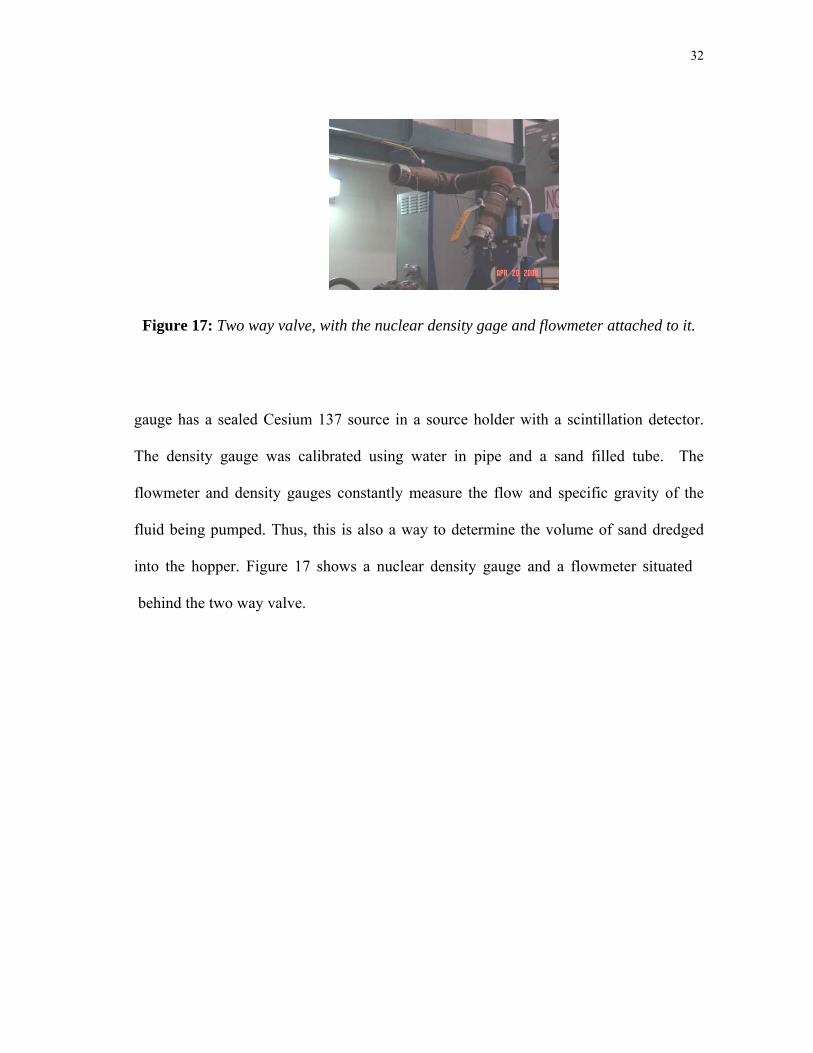
Figure 17: Two way valve, with the nuclear density gage and flowmeter attached to it.  

gauge has a sealed Cesium 137 source in a source holder with a scintillation detector.

The density gauge was calibrated using water in pipe and a sand filled tube. The

flowmeter and density gauges constantly measure the flow and specific gravity of the

fluid being pumped. Thus, this is also a way to determine the volume of sand dredged

into the hopper. Figure 17 shows a nuclear density gauge and a flowmeter situated

behind the two way valve.

33

CHAPTER V

EXPERIMENTAL PROCEDURES

5.1 Procedures for Experimental Measurements

Figure 18: General set up of the experiment.  

The sediment is uniformly spread before every test, and a laser profiler is run

over the sediment pit. The laser profiler records the z-distance from the head (from

where the LASER beam is emitted) to the sediment pit. This data is stored as a text file.

The tank is then filled up to six feet of water. The hopper is kept empty. This is ensured

by using sump pumps to keep the water out of the hopper. The dredge pump on the

34

carriage is then primed, which may take 15 to 20 minutes. After priming, the pump is

kept running until the test is complete. Next, the flow rate is set and the specific gravity

is measured. Once the pumping starts, care is taken such that the suction of the pump is

not above the sediment bed to avoid the suction of sediments before the actual dredging

operation begins. The water from the pump is discharged back to the tow tank initially.

Once the cutter starts dredging, the dredged sediments are directed to the hopper barge.

Table 4 shows the test parameters while Figure 18 shows the experimental set up at the

Haynes Laboratory.

Table 4: The test matrix for the 7 day testing period

DAYS DAY 1

Jul 12

DAY 2

Jul 16

DAY 3

Jul 17

DAY 4

Jul 18

DAY 5

Aug 25

DAY 6

Aug 27

Test Parameters

Flow rate (GPM) 200 200 150 150 200 200

Cutter rpm 86 86 86 86 86 86

Depth of Cut(inches)

8,10,12 8,10,12 8,10,12

8,10,12 8 8

Filled till overflow

Ladder angle (deg) 26 26 26 26 32 32

Once the flow rate and the cutter speed are set, the carriage moves in a

predefined path along the sediment pit. The depth is defined by the operator at the start

of every cut. At the beginning of the dredging process, the slurry is directed into the

35

hopper by using a Y valve, which switches the flow. The dredge carriage was automated

for the last two tests and eight cuts were made along the sediment pit. The motion of the

dredge carriage and the geometry of the cutter are as shown in Figure 19.

Figure 19: Schematic of the volume of sand removed when moving from A to B (left) Motion of the cutter suction dredge (right).

When the hopper is filled to overflow, the ladder is raised and once the Specific

Gravity (SG) goes back to 1.0, the pumping is stopped. The data from the pressure

gauges are measured and the SG is recorded. The hopper is disconnected from the

carriage and moved to the extreme end of the tank. A screen is kept between the

sediment pit and the hopper so as to avoid mixing. The bottom doors of the hopper are

then opened to discharge the sand on the bottom of the tank. The water is then drained

B 

C 

A 

48” 

Tow Tank Wall 

144”

Start 

End 

Initiation of the sediment pit 

33

10.5” 

8” = Depth of Cut 

B

A 

32deg13.5”

6”

10.5”

12.9”

36

and the hopper is rested on the bottom of the tow tank. The sediment pit is dewatered

using sump pumps, so as to run the laser profiler effectively. The laser profiler is run on

the sediment pit as well as the sand dropped from the hopper. The data (text files) from

the laser profiler are inputs to a MATLAB code that determines the volume of sand

removed by the cutter as well as material in the hopper respectively. The hopper is

cleaned, the released sand is shoveled back to the pit, and the tank is ready for the next

test run.

The motion of the dredge as described in Figure 19 gives an idea as to what the

production is even before the tests are conducted. This may not be the actual value of the

production, but is a theoretical estimate based on the geometry of the cut. The distance

that the dredge traverses, depth of cut, the cutter dimensions, and the angle of the

articulating ladder on which the cutter is mounted are the inputs to this calculation.

The tests conducted on August 25 (Day6) and on August 27(Day 7) were tests for

repeatability. The carriage movement was automated. The ladder, as it reached the

position where dredging was initiated, was lowered to a set depth of 8in. The

predetermined path in which the carriage, hence the cutter moved is as shown in Figure

19.

37

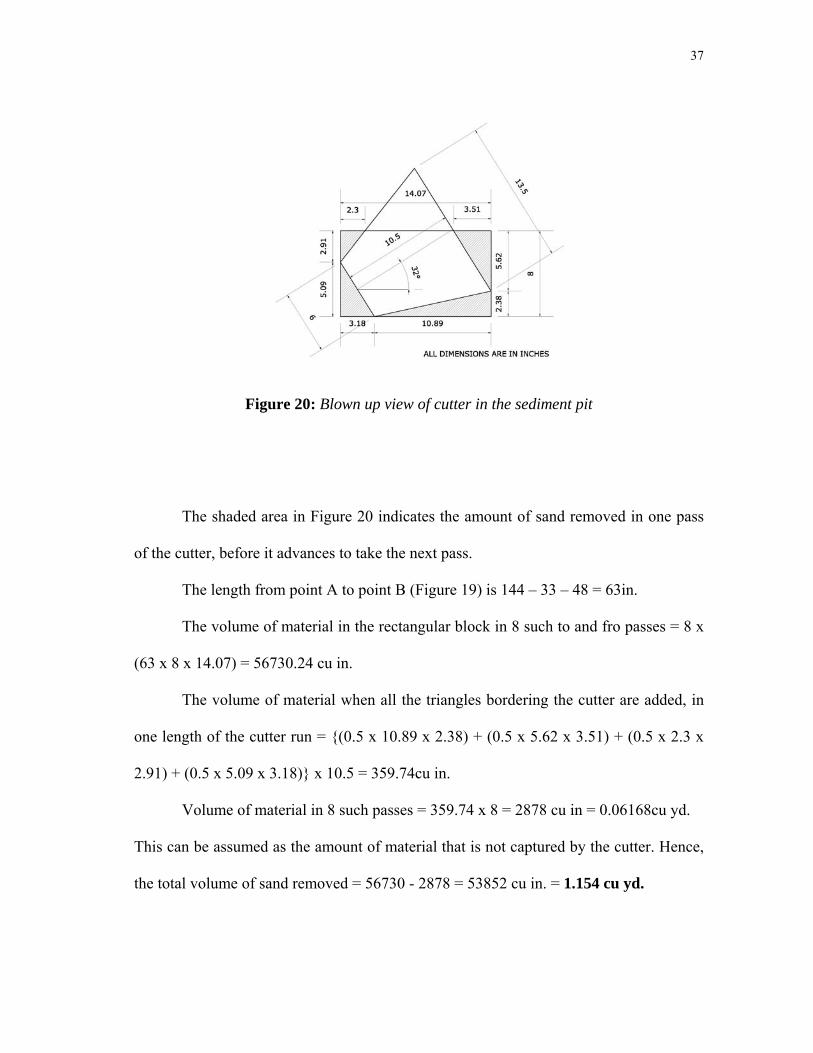
Figure 20: Blown up view of cutter in the sediment pit

The shaded area in Figure 20 indicates the amount of sand removed in one pass

of the cutter, before it advances to take the next pass.

The length from point A to point B (Figure 19) is 144 – 33 – 48 = 63in.

The volume of material in the rectangular block in 8 such to and fro passes = 8 x

(63 x 8 x 14.07) = 56730.24 cu in.

The volume of material when all the triangles bordering the cutter are added, in

one length of the cutter run = {(0.5 x 10.89 x 2.38) + (0.5 x 5.62 x 3.51) + (0.5 x 2.3 x

2.91) + (0.5 x 5.09 x 3.18)} x 10.5 = 359.74cu in.

Volume of material in 8 such passes = 359.74 x 8 = 2878 cu in = 0.06168cu yd.

This can be assumed as the amount of material that is not captured by the cutter. Hence,

the total volume of sand removed = 56730 - 2878 = 53852 cu in. = 1.154 cu yd.

38

The volume of sand removed calculated is the amount of material “supposed” to be

removed by the dredging process. There are losses due to turbidity and resuspension,

residuals, spillage, etc which results in lesser volume of material being actually removed.

This value may vary largely based on the cutter speed and the direction of the cut.

5.2 Calculation of Time Required

Before the test, the expected time required to run the test is calculated. If the

slurry is pumped at a rate of 300gpm (i.e. 0.024cu yd/sec), then, the time experiment was

calculated. This calculation was in line with the actual run time for the experiment. The

capacity of the hopper is 20.81cubic yards. If the slurry is pumped at a rate of 20gpm

(i.e. 0.0161cu yd/s), then, the time required for the hopper to fill up is 22 minutes

required for the hopper to fill up is 15 minutes. The additional standard set up times that

are added to the time required to fill the hopper up are listed in Table 5 below.

Table 5: The expected time required for testing  

Activity Time (min)

Time required for priming the pump 30

Time elapsed by the dredging operation till the time we get slurry in the discharge 30

Time required for removing the water from the sediment pit after dredging 120

Time required for setting and record the quantity of sediments dredged using the laser profile system

60

Time require d for pumping the sediment back to the pit and leveling the sediments 60

Time required for filling the channel back with water 120

39

Total time required for the test is approximately eight to nine hours, including the time

for data Acquisition.

5.3 Problems During Set Up and Testing

When attempting to release the sediments from the bottom of the hopper by

opening the doors, the buoyancy of the doors did not allow them to open. This problem

was overcome by clamping lead blocks to the doors of the hopper. These lead blocks

increased the weight of the doors leading them to open wide when the winches were

lowered during the release of the sediments. The area where the dredged sediments are

dropped from the hopper barge is not too far from the sediment pit. For that reason,

during the first experiment, it was very difficult to determine the boundary between the

sediment pit and the sediments dropped from the hopper. Hence, determining the area

that the laser needs to cover became difficult. This difficulty was overcome by placing a

screen between the sediment pit and the area where the sediments from the hopper were

dropped. The screen thus defined the two areas as shown in Figure 21.

40

Figure 21: The filter being placed between the hopper and sediment pit (left) The bottom of the tow tank after the filter is removed (right).  

Previous experiments by Henriksen and Randall (2007), for calculating

resuspension, suggested the use of a frame for holding the laser profiler so as to avoid

the possibility of the laser profiler sinking into the sediments as the readings are being

taken. Such a frame was fabricated in the laboratory and is shown in Figure 22. As the

sediments were pumped into the hopper the hose had a tendency to sway

dangerously. This problem was solved by attaching the hose rigidly to the hopper by

means of clamps as shown in Figure 22.

41

Figure 22: Laser Profiler on the frame, hanging from the top of the tow tank (left) Hose attached to the hopper barge (right).

5.4 Experimental Methods

Four different approaches were used to find the amount of sediments dredged. The

approaches are the following:

1. Using the Laser profiler over the before (flat) and after (dredged)

bathymetry of the sediment pit.

2. Using the Laser profiler over the sediments placed on the surface of the

tow tank from the hopper.

3. Using pressure gauges attached to the model hopper barge.

4. Using the flow meter and the density gauge on the carriage.

Each of the methods is explained separately in the next section.

42

CHAPTER VI

DATA ANALYSIS

6.1 Method A: Using the Laser Profiler over the Sediment Pit

The sediment pit is smoothened every time prior to the test, and is made flat before

the next test begins. The laser is mounted on the sediment pit such that the laser can

cover the area of the sediment pit that would be dredged. Necessary connections to the

computer are made. Inputs to the laser such as the laser area and the x and y increments

at which the data are recorded are given using computer software. The laser takes the

depth readings at each 5mm and 20 mm x and y increments, respectively. The software

generates a text file and a notepad file for every run of the laser.

Figure 23: A profile of the sediment pit (left), generated by MATLAB; the eight cuts can be distinctly seen (Test 7).

These data are input to the MATLAB code which returns the user with the

volume of sediments dredged. The MATLAB code generates a flat profile of the

43

sediment pit. Similarly, the laser is run to know the new depths of the sediment after the

dredging operation is completed. The depth data before and after the dredging operation

are an input to the MATLAB program, which generates the transect of the sediment pit

and the profiles of the sediment bed before and after the dredging process. The

MATLAB also calculates the volume of the sediments removed. Figure 23 shows the

actual picture of the pit as well as the profile generated by MATLAB after dredging.

The results obtained from this method are shown in Table 6.

Table 6: Volume of sand removed using the laser profiler over the pit

Test Date July 12 July 16 July 17 July 18 August 25 August 27

Volume of sand removed in yd3

0.4432 0.4444 0.8572 0.9894 0.4433 0.4334

Volume of sand removed in m3

0.3388 0.3397 0.6553 0.7564 0.3389 03313

With the parameters changed there is a marked difference in the tests on July 17, July

18 and the tests on July 12, July 16, August 25 and August 27. In the test experiments on

July 12 and July 16 the hopper was filled to overflow. But most of the sediments fell

back to the pit, due to leakage or spillage.

44

6.2 Method B: Using the Laser Profiler over the Sediments Placed on the Surface of the

Tow Tank from the Hopper

The dredged sediments are continuously pumped into the hopper as the dredging

process is conducted. After the dredging operation is completed, the hopper is moved to

the extreme end of the tow tank, and the hopper doors are opened to release the

sediments on the bed of the tank. The hopper is then disengaged from the carriage and

moved to a position over the jacks, where it sets after the water is drained. The water is

then drained and the sand released from the hopper is piled up so that it is contained in

the laser area. The laser area is set and the depth readings are taken using the laser. A

laser run of the flat surface of the tow tank is also taken. This data serves as an input to

the MATLAB code that gives us an output in terms of the volume. The MATLAB

generated image and the actual image are juxtaposed in Figure 24. The results from this

method are shown in Table 7.

Figure 24: A profile of the dropped sediments generated by MATLAB; the eight cuts can be distinctly seen.

45

Table 7: Volume of sand removed using the laser profiler over the pile

Test Date July 12 July 16 July 17 July 18 August 25 August 27

Volume of sand removed in yd3

0.2903 0.4197 0.3263 0.2135 0.2903 0.3927

Volume of sand removed in m3

0.2219 0.3208 0.2494 0.1632 0.2219 0.3002

Similar to the previous method, the differences in volume are seen. There is a

consistent difference seen here too. The reason as why a difference is seen is explained

in the next chapter.

6.3 Method C: Using Pressure Gauges Attached to the Model Hopper Barge

A valve, on the carriage, that was used to pump the dredged sediments was replaced

by the two way valve (Figure 25). Hoses are attached to the two-way valve, and one

hose is directed back to the tow tank (valve 1), while the other is directed to the hopper

(valve 2). The pump is primed with the valve 2 closed and valve 1 open. When the

dredging operation begins, valve 2 is opened and valve 1 is shut simultaneously. This is

done when the density of the dredged sediments increases as the cutter starts to cut into

the sediments. The amount of sand removed during dredging is determined using draft

measurements outside the hopper barge. The amount of sand and water inside the

hopper is determined from the internal height (Im) measured vertically as illustrated in

46

Figure 25. The calibrated pressure gauges provide measurements corresponding to the

variations in the load. The hopper draft (h) is calculated by averaging the values from the

four pressure gauges.

hIm

slurry levelwater level

Figure 25: The two way valve on the carriage (left) Schematic of model hopper (right).

The total weight of the hopper (Wt) is

iet WWW += (9)

where We is the weight calculated from the pressure gauge reading when the hopper is

empty and Wi is the weight of the slurry in the hopper. The total weight of the hopper is

also the displaced volume of the hopper multiplied by the specific weight of the water in

the dredge/tow tank

dwt VγW = (10)

47

where Vd is the displaced volume of the hopper and γw is the specific weight of water.

The draft of the hopper (h) and the weight per unit draft (m1) of the hopper displacement

are defined by

dw1

Vγmh

= (11)

The relationship between the draft (h) and the hopper total weight is illustrated in

Figure 26, where m1 is the slope of the line.

0

5

10

15

20

25

0 5000 10000 15000 20000 25000 30000

Draft of the ho

pper (in)

Total weight of hopper (lbs)

Figure 26: Graph showing the increase in weight of the hopper as draft (h) changes.  

The total weight of the hopper and dredged slurry is

1iet m

hWWW =+= (12)

The volume of the slurry inside the hopper is the sum of the volume of sand (Vs)

and water (Vw), and it is determined by the height of the slurry in the hopper. Based on

48

the geometry of the hopper, the volume of the hopper can be divided into two parts, a

cuboid (Vc) and a frustum of a pyramid (Vp). Imp is the height of the frustum of a

pyramid, while Imc is the height of the slurry in the cuboid.

cmcpmppcws mImIVVVV +=+=+ (13)

The volume Vp and Vc are plotted against the respective heights, Imp and Imc and

the slopes mp and mc are determined (Figure 27).

0

50

100

150

200

250

300

0 10 20 30 40 50 60

Volume (cu ft)

Height  of slurry in the hopper (inches)

Figure 27: Graph showing the change in volume of the hopper as Im changes.  

The volume of sand (Vs) in the hopper is determined using

1SG

ImImγW

mγh

Vmccmpp

w

e

1ws −

−−−= (14)

mp 

mc 

49

where SG is the specific gravity of the sand. An example calculation of the sand volume

using one of the pressure sensors (sensor #1) is shown in Table 8. Similarly, the volume

of sand for sensor #4 was found to be 0.191m3 (0.250yd3). There were four pressure

sensors mounted on the hopper barge with # 1 and #2 at the bow and stern respectively

and #2 and #3 centered at the port and starboard. Pressure sensor #3 malfunctioned

during the tests so only the sensors #1 and #4 (bow and stern) were used, and the

average of the two volumes results in average volume of 0.261m3 (0.342 yd3).

Table 8: Example calculation of dredged sand volume for pressure sensor #1  

Wt

kg

(lb)

h

m

(in)

m1

m/kg

(ft/lb)

Imc

m

(in)

Imp

m

(in)

Vp

m3

(ft3)

Vc

m3

(ft3)

mc

m3/m

(ft3/ft)

mp

m3/m

(ft3/ft)

Vs

m3

(yd3)

21510.1 18.8 7.29E-05 29 15 60.47 140 23.24 112 0.435

9756.83 0.478 4.89E-5 0.737 0.381 1.712 3.96 2.159 10.41 0.332

6.4 Method D: Using the Flow Meter and the Density Gauge on the Carriage

The flowmeter on the carriage is also used to determine the volume of sediments

pumped into the hopper. The flowmeter records the flow in GPM of the sediments while

the density gauge measures the specific gravity of the slurry every second as it is

50

pumped into the hopper. The production (cubic meters/hr or cubic yards/hr) is

calculated using the following equation,

QCP v= (15)

where Cv is the concentration by volume and Q is the flowrate. The concentration by

volume is

1SG1SGC

solids

sv −

−= (16)

where SGs is the measured slurry specific gravity being pumped by the model dredge

and SGsolids is the specific gravity of the insitu sand. This is used to calculate the

instantaneous production of sand and the instantaneous production is integrated over

time to give the total production of insitu sand. This process is illustrated in Figure 28

where the flowrate (red line) and specific gravity (blue line) are used in equations 15 and

16 to calculate the instantaneous production for the slurry (green line) and sand (purple

line). The instantaneous production shown in the graph was integrated using MatLab to

get total production of sand using a specific gravity of 1.65 that resulted in a total insitu

production of 0.196m3 (0.256yd3).

51

‐5

0

5

10

15

20

25

0 50 100 150 200 250 300 350 400 450 500

Time (s)

Flow(ft/s)Production(cu.yd/hr) ‐ slurryProduction(Cu.yd/hr) ‐ sandS G *10

Figure 28: An example of the production plot while discharging slurry into hopper barge during dredging with model cutter suction dredge.

The production values of sand computed using different values of SG in the

expression for calculating the concentration factor (Cv), are listed in Table 9.

Table 9: Values of production in Cu Yd for different values of SG  

Values of SG used in expression for Cv

Test 1

12 July

Test 2

16 July

Test 3

17 July

Test 4

18 July

Test 5

25 August

Test 627 August

2.1 1.083 1.293 0.354 0.315 0.150 0.209

2 1.192 1.422 0.390 0.347 0.165 0.230

1.9 1.324 1.5801 0.433 0.385 0.183 0.256

1.8 1.489 1.778 0.487 0.433 0.194 0.288

1.7 1.702 2.031 0.557 0.495 0.206 0.329

1.6 1.986 2.370 0.649 0.578 0.275 0.384

52

CHAPTER VII

SUMMARY AND DISCUSSION OF RESULTS

7.1 Summary and Discussions of Results from All the Tests  

The Table 10 summarizes all the values from the various methods used in the study

(Method A, Method B, Method C and Method D). A direct comparison can be made

between various methods by looking at the table. 

Table 10: Summary of results from all the methods

Test Date July 12 July 16 July 17 July 18 August 25 August 27

THE VOLUME OF SAND REMOVED IN CUBIC YARDS

Laser over pit (A) 0.443 0.444 0.857 0.989 0.443 0.433

Laser over pile (B) 0.290 0.420 0.326 0.213 0.290 0.392

Hopper draft (C)

4.27 1.117 5.84 5.635 0.343 0.335

Flowmeter and Density Gauge (D)

SG July 12 July 16 July 17 July 18 August 25 August 27

2.1 1.083 1.293 0.354 0.315 0.150 0.209

2.0 1.192 1.422 0.390 0.347 0.165 0.230

1.9 1.324 1.5801 0.433 0.385 0.183 0.256

1.8 1.489 1.778 0.487 0.433 0.194 0.288

1.7 1.702 2.031 0.557 0.495 0.206 0.329

1.6 1.986 2.370 0.649 0.578 0.275 0.384

53

The first set of raw data was processed from tests conducted on July 12, 16, 17 and

18 of 2008. There were some problems and errors found during the tests and, after data

processing, a few others were revealed. These first four tests paved the way for the two

final, successfully completed tests. The tests on the 12 and 16 of July were similar tests

in that their flowrates were set at 200 gpm, and the tests on the 17 and 18 had flowrates

of 150gpm. Amongst all the results obtained from various methods, Method D (using

flow meter and density gauge) shows a fairly accurate value of the sediments dredged,

for the value of SG used in the equation of Cv.

The results from Method C (using the pressure gauges) are not in agreement with

the Method D (using flow meter and density gauge). One of the reasons being, at the

beginning of the dredging process, the recording of data from the pressure gauges was

not simultaneous with the switching of the valves. The first readings from the pressure

gauges were recorded when the team thought that the slurry pumped had enough

sediment or, in other words, the cutter started cutting through sediments. Thus, when the

first reading was taken, the hopper already contained water and sediments and the exact

weight of the empty hopper (We) at the beginning of the experiment was not known.

The leakage of the hopper was evident during the second experiment when the

slurry level inside the hopper kept dropping significantly as the dredging experiment

continued and the hopper was continuously filled. Attempts to prevent leakage by

tightening the winches in the third and fourth tests did not help to reduce the leakage

significantly. Most of the material leaked and was deposited on the bottom of the tank

before the sediments were dropped into the sediment pit. This problem was eliminated in

54

the last two tests by sealing the hopper doors with a simple window sealant. Thus, even

though the hopper was filled up to overflow in the first four tests, the values of the

volume of sediments dredged from method B is too low when compared to the value

from the flow meter and density gauge (method D). While method A shows a lesser

value, it is speculated that some sediments must have deposited back on to the sediment

pit due to leakage.

This experiment experienced problems identifying the sediments that were

originally in the sediment pit after dredging versus sediments from other sources. In the

first four tests, leakage and resuspension were present, creating anomalies. In the final

two tests, the issue of the leaked sediments from the hopper was resolved, but spillage

was still a matter of concern.

The last two tests were completed with all the known problems corrected. In

addition to the changes made, the carriage movement was automated and a uniform cut

depth of 8in was used. The angle of the articulating ladder was also increased from 26

deg to 32 deg. The results obtained from the methods B and C are in close agreement

with each other. They are also in line with the method D, when the Cv is calculated with

an SG in the range of 1.6 to 1.7. However, there is a difference seen in A and the

difference is consistent in both methods. During the dredging operation, spillage occurs

and sand is deposited (piles up) on both the sides of the sediment pit. This increases the

dredged area, which in turn increases the values of sediments dredged from the sediment

pit (Method A), when compared to other methods.  

55

CHAPTER VIII

CONCLUSIONS AND RECOMMENDATIONS

It is seen in the last two tests that the hopper and its instrumentation functioned

well. The results from the pressure gauges attached to the model hopper barge were

more accurate in the last two tests than the first four tests. However, it is recommended

to thoroughly check the pressure gauges for operation and the hopper doors for caulking,

and to take few pressure readings before the water is pumped in the hopper.

The results (volume of sediments dredged) from method D in the tests conducted

on July 12 and 16 is much greater compared to those from July 17 and 18; the reason

being the hopper was filled till overflow in the first two tests. The increase in the angle

in the last two tests, from 26 deg to 32 deg, and the reduction of the depth to 8 inches

also reduced the bulldozing of the cutter in the tests conducted on the 25 & 27 of

August.

As explained in the previous chapter, some sediments fall outside the laser

profiler’s area in the sediment pit once the dredging is done, due to the cutter action.

This increased the amount of sediment dredged from the sediment pit (method A), when

compared to the values obtained from running the laser profiler on the sediments

dropped from the hopper barge (method B). The difference is the spillage that occurs

during dredging. Thus, the laser profiler is a good device in determining the spillage, but

the value of spillage computed by this method need not be completely accurate. The

inaccuracy in the spillage values could be due to the following reasons:

56

1. The specific gravity of the sand in the sediment pit is different from that of the

sediments dropped from the hopper. The sediments dropped from the hopper are

shoveled and moved into the laser profiler area and, in this process, the sand

loses a lot of water content.

2. The laser profiler is subjected to reflection from the water present in the pit, as all

the water could not be pumped out (excessive pumping leads to loss of

sediments). The use of an acoustic profiler should be investigated. Such a system

would not require the water to be removed. This would save water and speed up

the testing procedure.

It is also recommended to reduce the area of the cutter movement (sideways) and

wait until the water in the pit dries up before running the laser profiler. This would

eliminate the issue of sediments settling outside the laser area and avoid the reflection of

the laser from the water. This method is costly in time as well as money; hence, a better

alternative needs to be thought of.

These experiments clarify various aspects of dredging. Many issues in laboratory

testing are pointed out and solutions are provided. The instrumentation on the hopper

was successful. This method also serves as a comparison with various methods of

dredging. The laser profiler also serves instrumental in calculating the spillage of sand.

More experiments with corrected procedures and varying input parameters need to be

conducted. This would clarify the effects of parameter variation on the dredging process.

Due to time constraints and other commitments, the effects of changing input parameters

could not be studied.

57

REFERENCES

Armstrong, P.L. and Grant, M.E. (1977) “Dredging Spoil Measurement Device”, Dock and Harbor Authority, June 1997. Brahme, S.B. (1983). “Environmental Aspects of Suction Cutterheads.” Dissertation, Ocean Engineering Program, Civil Engineering Department, Texas A&M University, College Station, Texas. Burger, M. den, Vlasblom, W.J., Talmon, A.M.(2005) “Design Aspects for Cutterheads Related to the Mixture Forming Process When Cutting Coarse Materials” Terra et Aqua, number 98, mart 2005, blz 12-18 ISSN 0376-6411. Fortino, E.P. (1966) “Flow Measurement Techniques for Hydraulic Dredges”, Journal of the Waterways and Harbors Division, Proceedings of the ASCE, Vol.92, pp 109-125. Glover, G.J., (2002) “Laboratory Modeling of Hydraulic Dredges and Design of Dredge Carriage for Laboratory Facility”, Master of Science Thesis, Texas A&M University, Ocean Engineering Program, Department of Civil Engineering, College Station , TX, December 2002. Glover, G.J. and Randall, R.E., (2004). “Scaling of Model Hydraulic Dredges with Application to Design of a Dredge Modeling Facility”, Journal of Dredging Engineering, Western Dredging Association (WEDA), vol. 6, no. 2, pp. 15-36, September. Henriksen, J., Randall, R.E., deJong, P, and Sonye, S., (2007) “Initial Experiments and Data Acquisition for the Model Dredge Carriage”. Proceedings of the World Dredging Congress XVIII, Paper 6C-6, Lake Buena Vista, FL, USA, May 27-June1. Herbich, J.B., (2000) “Handbook of Dredging Engineering”, Second Edition, McGraw-Hill, New York, NY. Herbich, J.B & Brahme, S.B (1983) - “Literature Review and Technical Evaluation of Sediment Resuspension on During Dredging”, Report No. COE-266, Center for Dredging Studies, Texas A&M University, College Station, Texas. Huston, J.W., and Huston, W.C. (1976) “Techniques for Reducing Turbidity with Present Dredging Procedures and Operation.” Technical Report D-76-4, U.S Army Engineering Waterways Station. Vicksburg, MS.

58

Joanknecht, L.W.F. (1976) “A Review of Dredge Cutterhead Modeling and Performance”, Proceedings of the Seventh World Dredging Congress, WODCON VII, San Fransisco, CA. Meyer, G.M, Meynard, Granboulan and Babylon, (1986) “A Study of Decantation of Fine Sediments in a Trailing Suction Dredging Hopper with the Aid of a Photon Emitting Probe.” Proceedings of the XIth World Dredging Congress, Brighton, United Kingdom. Miller, J., Palmero, M., and Groff, T. (2001), “Hopper Overflow Characteristics of the Delaware River”, Journal of Dredging Engineering, Western Dredging Association (WEDA),. vol.3, no.1, pp.1-20, March. Palermo, M.R. and Randall R.E., (1989) “Economic Loading and Overflow for Dredge Scows and Hoppers”, Proceedings of World Dredging Congress, WODCON XII, Orlando, FL, May 1-5. Rokosch, W.D, Van Vechgel, R.H.L and van der Veen, R. (1986), “Analysis of Mixed Hopper Loads in Dredging.” Proceedings of the XIth World Dredging Congress, Brighton, United Kingdom. Slotta, L.S. (1968) “Flow Visualization Techniques Used in Dredge Cutterhead Evaluation.” Proceedings of the 1968 World Dredging Congress, WODCON XV, Las Vegas, NV. Schroeder, P.R., (2009) “USACE Technical Guidelines for Practicing the 3R’s of Environmental Dredging”, Proceedings of the Western Dredging Association Twenty-ninth Technical Conference and 40th Annual Texas A&M Dredging Seminar, Tempe, AZ, June 2009.  

59

APPENDIX

1. The MATLAB Program for the laser profiler data

clc;clear;

%

xyz1 = load('predredgefinal.dat'); %Topography of pre-run

xyz2 = load('postdredgemonone.dat'); %Topography of post-run

%Input

x_min = 5; x_max = 5000; x_resolution = 5; %1st, end points and Resolution

y_min = 0; y_max = 2500; y_resolution = 20; %1st, end points and Resolution

dh = 20; %Threshold in Despiking

%End of Input

%---------------------------------------------------------------

%MATLAB data structure

flag_x = (x_max-x_min)/x_resolution+1;

flag_y = (y_max-y_min)/y_resolution+1;

for i = 1:flag_x

x(i) = x_resolution*i;

end

for i = 1:flag_y

y(i) = y_resolution*(i-1);

end

% Building the actuall z array for plotting

for j = 1:flag_y

for i = 1:flag_x

60

k = (j-1)*flag_x + i;

z1(j,i) = xyz1(k,3);

z2(j,i) = xyz2(k,3);

end

end

z3 = z2 -z1;

%End of Task

%Despike

nz1 = despike(z1,dh); nz2 = despike(z2,dh); nz3 = despike(z3,dh);

%End of Task

%Output Figures

figure(1)

surf(x,y,nz1)

title('Topography before the Test');

xlabel('x (mm)'); ylabel('y (mm)'); zlabel('z (mm)');

xlim([x_min x_max]); xlim([y_min y_max]);

axis equal

figure(2)

surf(x,y,nz2)

title('Topography after the Test');

xlabel('x (mm)'); ylabel('y (mm)'); zlabel('z (mm)');

xlim([x_min x_max]); xlim([y_min y_max]);

axis equal

figure(3)

surf(x,y,nz3)

title('Topography Changes in the Test');

xlabel('x (mm)'); ylabel('y (mm)'); zlabel('z (mm)');

61

xlim([x_min x_max]); xlim([y_min y_max]);

axis equal

%%%%%%%%%%%%%%%%%%%%%%%%%%%%%%%%%%%%%%%%%%%%%%%%%%%

%%%%%%%%%%%%%%%%%%%%%%%%%%%%%%%

%Now going to calculate the amount of material using an integral

%Lets first create the right matrixs for x and y for the program and

%plotting

for k=1:flag_y

for j=1:flag_x

xmatrix(k,j)=x(j);

end

end

for k=1:flag_x

for j=1:flag_y

ymatrix(j,k)=y(j);

end

end

volume= int_2D_tabulated(xmatrix,ymatrix, nz3 )

%Lets look at a transect of these profiles

for i=1:flag_x

transect1(i)=nz1(75,i);

transect2(i)=nz2(75,i);

end

for i=1:flag_x

xtransect(i)=i*5;

end

figure(4)

62

plot(xtransect,transect1)

title('Transect Profile');

xlabel('x (mm)');ylabel('z (mm)');

%Output File-------If you think it's too slow, you can delete this part.

% for i = 1:flag_y

% for j = 1:flag_x

% k = (i-1)*flag_x + j;

% Outxyz(k,1) = x(j);

% Outxyz(k,2) = y(i);

% Outxyz(k,3) = nz1(i,j);

% Outxyz(k,4) = nz2(i,j);

% Outxyz(k,5) = nz3(i,j);

% end

% end

% save -ascii Outxyz_2.dat Outxyz

63

VITA

Name: Arun Kumar Manikantan

Address: Texas A&M University, Ocean Engineering Program, MS: 3136, College Station, Texas, 77840

Email Address: [email protected]

Education: B.E., Mechanical Engineering, SPCE, Mumbai University, 2005 M.S., Ocean Engineering, Texas A&M University, 2009