Comparing horizontal path C n measurements over 0.6 ... - DTIC

Comparing horizontal path C2n measurements over 0.6 km in

the tropical littoral environment and in the desert

Mark P. J. L. Chang1, Carlos O. Font2, G. Charmaine Gilbreath2, Eun Oh2,Emi Distefano2, Sergio Restaino3, Christopher Wilcox3 and Freddie Santiago4

1Physics Department, University of Puerto Rico, Mayaguez, Puerto Rico 00680.2U.S. Naval Research Laboratory, Washington D.C. 20375.

3U.S. Naval Research Laboratory West, Albuquerque, New Mexico.4P.O. Box 2114, Guaynabo, PR 00970-2114.

ABSTRACT

We have measured the optical turbulence structure parameter, C2n, in two extremely different locations: the first

being the littoral region on the southwest coast of Puerto Rico. The second location is over the dry desert incentral New Mexico. In both cases, the horizontal beam paths are approximately 0.6 km long, within 2 metersof the local surface (Puerto Rico) and varying between 2 to 100 meters (New Mexico). We present our findingsfrom the two datasets.

Keywords: Strength of Turbulence Parameter, Scintillation, Littoral Turbulence, Desert Turbulence

1. INTRODUCTION

We have obtained weak turbulence optical C2n measurements, integrated over 600m horizontal paths in both

the littoral environment in the Caribbean region (southwest Puerto Rico) and in the high desert of central NewMexico. The Puerto Rico littoral data record covers the period between February 4 to March 13, 2007 (yeardays 35 to 72). The New Mexico record is more limited, covering only March 5 to March 9, 2007 (year days 95to 99). The instrument systems used are identical OSI LOA-004s, described in previous reports.1–3

For convenience, we designate the littoral measurement campaign as VIPh in this paper; results of a previous(2006) campaign at the same site have been reported recently.4 The New Mexico measurements took place atthe Starfire Optical Range, Albuquerque and we reference them with the abbreviation SOR.

The robust and repeatable mathematical properties of a variable are sometimes referred to as “stylised facts”.In this paper we seek to establish some of the stylised facts of our observations; the structure of the documentis as follows: In Section 2 we present a summary of the VIPh measurements over the 37 days and what we havelearned from this record. We follow this with a discussion of the 5 days of desert measurements. We observethe expected temperature driven characteristics of weak, clear air turbulence in the time series measurements.In particular, we note that the SOR system exhibits features of a lognormal amplitude distribution throughoutthe entire record whereas the VIPh system is modified by a daytime component. In general we are concernedwith understanding these systems from the perspective of scaling. By identifying characteristic scales or scale–independent features, we will be better placed to discuss the various underlying physical processes contributingto the system variations. Moreover, quantitative comparitive studies between the time series records can bemade. With that in mind, we have analysed first and second order statistics. Specifically, we examine thefirst difference (or single decimation) of the C2

n measurements, the probability distribution function (PDF), theautocorrelation function (ACF) and the Hilbert Huang spectra. We list the observed stylised facts in Section 3and then conclude with Section 4.

Further author information: (Send correspondence to M.P.J.L.C.)M.P.J.L.C.: E-mail: [email protected], Telephone: 1 787 265 3844

Atmospheric Propagation IV, edited by Cynthia Y. Young, G. Charmaine Gilbreath,Proc. of SPIE Vol. 6551, 65510I, (2007) · 0277-786X/07/$18 · doi: 10.1117/12.718257

Proc. of SPIE Vol. 6551 65510I-1

Kate

Text Box

NRL Release Number 07-1226-1133

Report Documentation Page Form ApprovedOMB No. 0704-0188

Public reporting burden for the collection of information is estimated to average 1 hour per response, including the time for reviewing instructions, searching existing data sources, gathering andmaintaining the data needed, and completing and reviewing the collection of information. Send comments regarding this burden estimate or any other aspect of this collection of information,including suggestions for reducing this burden, to Washington Headquarters Services, Directorate for Information Operations and Reports, 1215 Jefferson Davis Highway, Suite 1204, ArlingtonVA 22202-4302. Respondents should be aware that notwithstanding any other provision of law, no person shall be subject to a penalty for failing to comply with a collection of information if itdoes not display a currently valid OMB control number.

1. REPORT DATE 2007 2. REPORT TYPE

3. DATES COVERED 00-00-2007 to 00-00-2007

4. TITLE AND SUBTITLE Comparing horizontal path C2n measurements over 0.6 km in thetropical littoral environment and in the desert

5a. CONTRACT NUMBER

5b. GRANT NUMBER

5c. PROGRAM ELEMENT NUMBER

6. AUTHOR(S) 5d. PROJECT NUMBER

5e. TASK NUMBER

5f. WORK UNIT NUMBER

7. PERFORMING ORGANIZATION NAME(S) AND ADDRESS(ES) Naval Research Laboratory,Code 8123, Advanced Systems TechnologyBranch,4555 Overlook Ave SW,Washington,DC,20375

8. PERFORMING ORGANIZATIONREPORT NUMBER

9. SPONSORING/MONITORING AGENCY NAME(S) AND ADDRESS(ES) 10. SPONSOR/MONITOR’S ACRONYM(S)

11. SPONSOR/MONITOR’S REPORT NUMBER(S)

12. DISTRIBUTION/AVAILABILITY STATEMENT Approved for public release; distribution unlimited

13. SUPPLEMENTARY NOTES

14. ABSTRACT We have measured the optical turbulence structure parameter, C2n , in two extremely different locations:the first being the littoral region on the southwest coast of Puerto Rico. The second location is over the drydesert in central New Mexico. In both cases, the horizontal beam paths are approximately 0.6 km long,within 2 meters of the local surface (Puerto Rico) and varying between 2 to 100 meters (New Mexico). Wepresent our findings from the two datasets.

15. SUBJECT TERMS

16. SECURITY CLASSIFICATION OF: 17. LIMITATION OF ABSTRACT Same as

Report (SAR)

18. NUMBEROF PAGES

9

19a. NAME OFRESPONSIBLE PERSON

a. REPORT unclassified

b. ABSTRACT unclassified

c. THIS PAGE unclassified

Standard Form 298 (Rev. 8-98) Prescribed by ANSI Std Z39-18

Year Day

—9

—10

—Il

C-)

—12

—13

—9

—10

—Ila

IS35 40 45 50 55 60 65 70 75

Year Day

2. DATA

2.1. VIPh (Puerto Rico) record

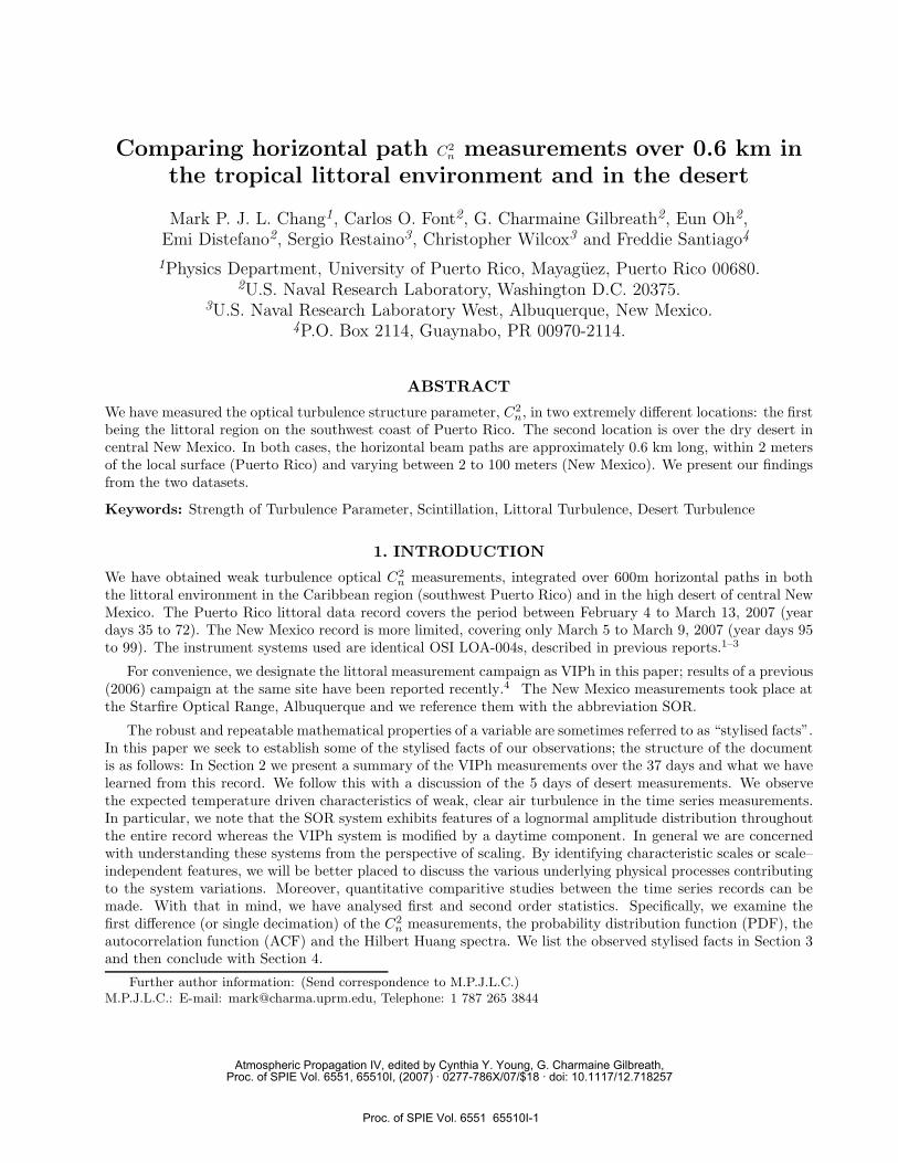
The near–infrared probe beam for these measurements was positioned at a mean height of 1.5 m above sealevel, aligned along a nearly North–South path of approximately 600 m length. The transmitter and receiversystems were placed at fixed locations on jettys for 32 out of the 37 campaign days (for more details on thedockside geometry, see Chang et al (2007)4). During the other 5 days, year days 43 to 47, the receiver systemwas placed on a moored, floating platform within 10 m to the south of its fixed position, with the aim of testingthe stability of its tripod mount in the presence of light tidal and wash effects. Although these 5 days’ worthof readings have a large C2

n baseline offset relative to the remaining days, we nevertheless include them in thediscussion as they provide visual continuity in Figs. 1 and 2.

Figure 1. The complete record of measurements over37 days for the VIPh campaign. Here, as in all subse-quent graphs, the integer day indicates midnight localtime.

Figure 2. The same data as Fig. 1, smoothed witha forward rolling average of 120 points including thedata gaps. Year days 42 to 47 clearly show the ef-fect of placing the scintillometer receiver on a floatingplatform. There is a strong, slow modulation on thebaseline. The physical cause of this modulation willbe explored elsewhere.

2.1.1. First Order Statistics: Differencing and PDF

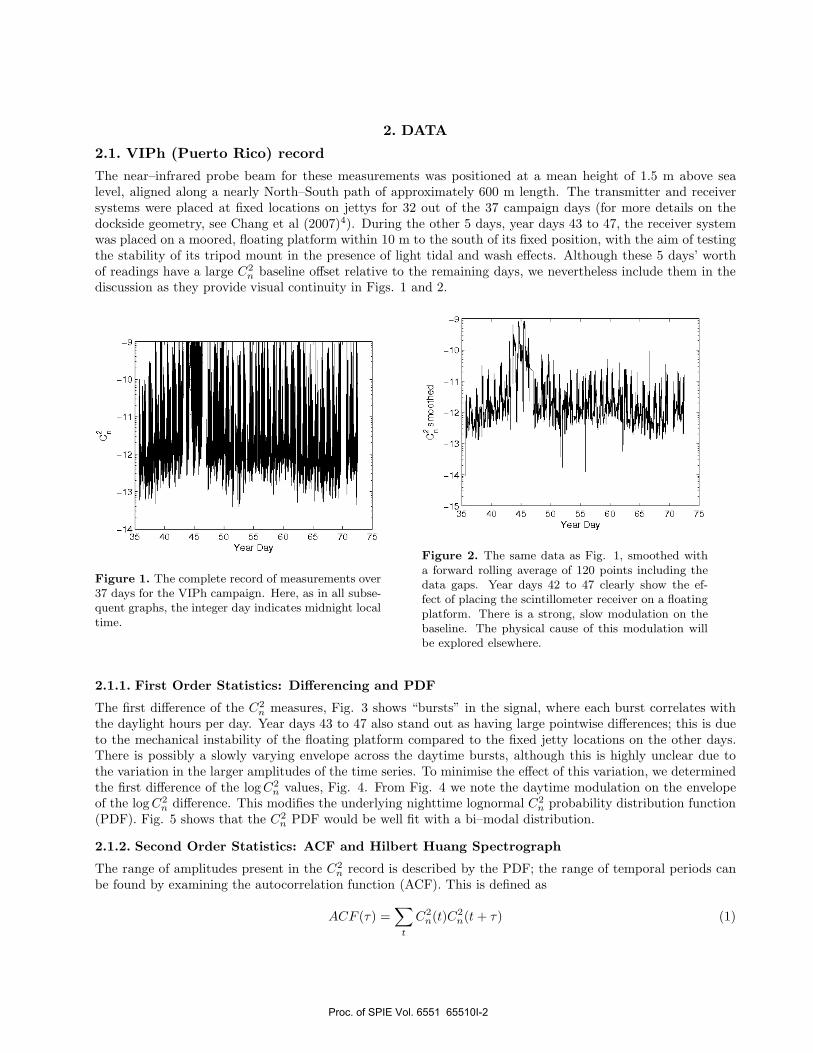
The first difference of the C2n measures, Fig. 3 shows “bursts” in the signal, where each burst correlates with

the daylight hours per day. Year days 43 to 47 also stand out as having large pointwise differences; this is dueto the mechanical instability of the floating platform compared to the fixed jetty locations on the other days.There is possibly a slowly varying envelope across the daytime bursts, although this is highly unclear due tothe variation in the larger amplitudes of the time series. To minimise the effect of this variation, we determinedthe first difference of the log C2

n values, Fig. 4. From Fig. 4 we note the daytime modulation on the envelopeof the log C2

n difference. This modifies the underlying nighttime lognormal C2n probability distribution function

(PDF). Fig. 5 shows that the C2n PDF would be well fit with a bi–modal distribution.

2.1.2. Second Order Statistics: ACF and Hilbert Huang Spectrograph

The range of amplitudes present in the C2n record is described by the PDF; the range of temporal periods can

be found by examining the autocorrelation function (ACF). This is defined as

ACF (τ) =∑

t

C2n(t)C2

n(t + τ) (1)


55

Year Day

i.."tf

40 45 50 55 60 65 70 75Year Day

D(C

2)

0

0 5 10 lb 20 25 30 35 40

Lag in Days

Figure 3. ∆C2n (single sample decimation) for the

VIPh data; note a possible modulation on the ampli-tude envelope.

Figure 4. ∆ log C2n (single sample decimation) for the

VIPh data; a rapidly modulated upper envelope canbe clearly discerned, showing the daytime effects uponthe data.

Figure 5. PDF of the VIPh C2n data record, using 10

000 bins, showing that a bi–modal fit is very appro-priate.

Figure 6. ACF of the VIPh C2n data record, truncated

on the vertical axis.


xl 0"

B10—x 58 80 B10—x 58

2.5 5

2 0

0.5

58 80 82 58 58 80 82

L11 I ILU. I L I 82

We show this in Fig. 6. The modulation atop the basic trend is again due to the solar heating during thedaylight hours. The ACF initially shows a rapidly dropping exponential followed by a long–range tail.

The frequency space version of the ACF is much less trivial to produce. The main obstacle is the non–stationarity of the time series, which does not allow us to use conventional algorithms such as the FourierTransform directly on the data.2 By windowing the data into “stationary” subsets as in Short Time FourierTransform techniques, it is possible to calculate a frequency map with a Fourier basis. However this tendsto have aliasing and resolution problems, since the basis representation is predefined. Fortunately the HilbertHuang Transform5 improves on this by defining the basis adaptively from the given time series via EmpiricalMode Decomposition. The components of the adaptive basis are known as the Intrinsic Mode Functions (IMFs).

The full data set has a large number of data gaps, primarily due to mechanical misalignments as theinstrumentation was unattended for long periods. Rather like the aliasing problem in Fourier methods, EmpiricalMode Decomposition is very sensitive to long breaks in the data stream,6 so the raw data is not ideal for spectralprocessing. We have therefore limited our spectral study to a subsection with few gaps.

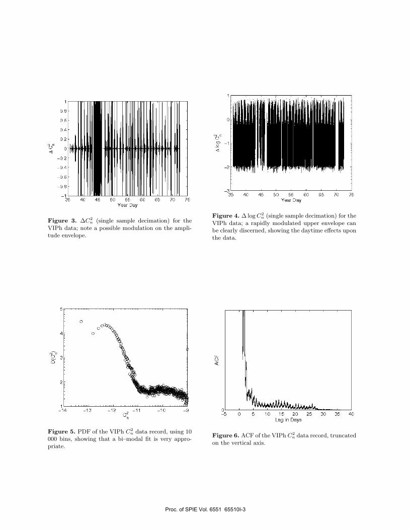
We show a 5 × 105 point subset of the data (covering approximately 6 days) in Fig. 7, in which the levelof lost data is less than 5%. 30 components were determined from the data (29 IMFs and trend), which arenotable by their division into 3 main orders of magnitude amplitude–wise: 10−10 (10 highest frequency IMFs),10−11 (next 15 IMFs) and 10−12 m−2/3 (lowest frequency IMFs and trend). The IMFs allow us to find a map

Figure 7. VIPh C2n data subset: [Upper panel] (Top to bottom, left to right) The trend; trend + lowest frequency IMF;

trend + 2 lowest frequency IMFs; trend + 3 lowest frequency IMFs. [Lower panel] The data subset used for spectralanalysis.

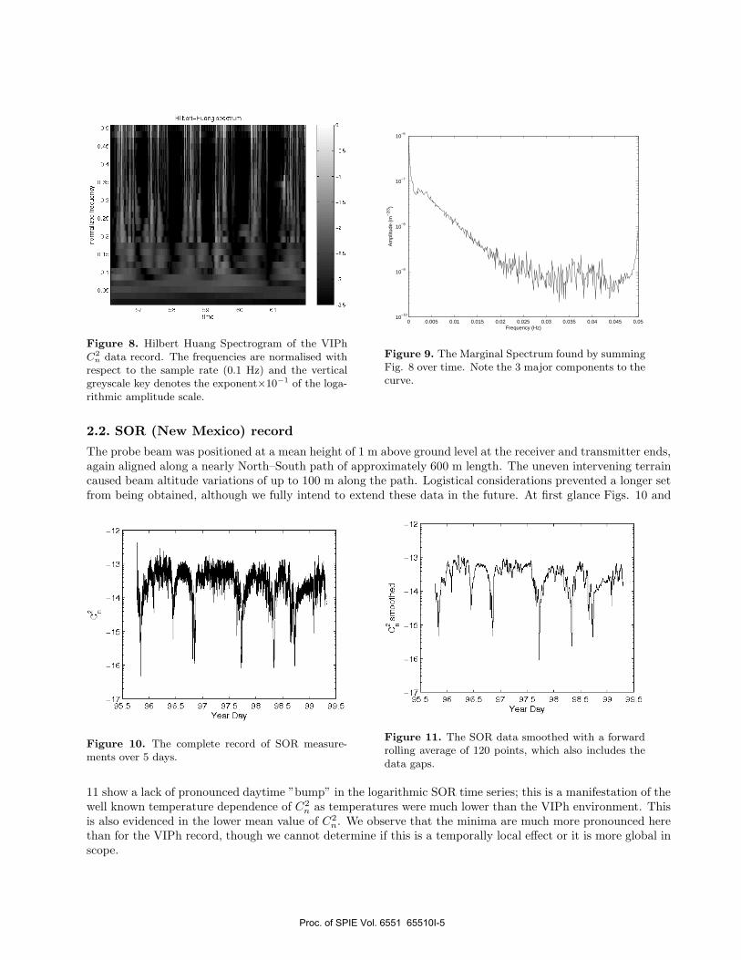
of instantaneous frequencies; this in turn generates the Hilbert Huang spectrogram (HHS). The HHS is a highresolution map in the time–frequency–amplitude domain, similar to a wavelet spectrogram. Fig. 8 shows theHHS for the data subset. We see that below approximately 5×10−3 Hz, the amplitudes are spread evenly acrossall time bins. Above this, the C2

n amplitudes are bunched into what is clearly the effect of solar insolation uponthe distribution.

The HHS map can be simplified by summing over the time axis to produce the (temporal) marginal HilbertHuang spectrum (Fig. 9). Though suggestive of a Fourier power spectrum, the points on the marginal spectrumrepresent the local probability of occurance of the frequencies. The curve has three major regions: (1) adecreasing ramp down to about 0.025 Hz, (2) a floor between 0.025 to 0.045 Hz and (3) a steep rise. Region(1) is potentially representative of the atmospheric activity in the absence of the Sun, being similar to Fig. 18.Region (2) is likely to be the result of the Sun’s action on the airmass. Region (3) is probably the result ofnumerical and/or instrumental noise, including the effect of the data gaps.


Hilben—Huang specifum

—12

—13

—14

—lb

—16

—1795.5 96 96.5 97 97.5 98 98.5 99 99.5

Year Day

—12

—13

—IS

—1796.6 96 96.5 97 97.5 98 98.5 99 99.5

Year Day

Figure 8. Hilbert Huang Spectrogram of the VIPhC2

n data record. The frequencies are normalised withrespect to the sample rate (0.1 Hz) and the verticalgreyscale key denotes the exponent×10−1 of the loga-rithmic amplitude scale.

0 0.005 0.01 0.015 0.02 0.025 0.03 0.035 0.04 0.045 0.0510

−10

10−9

10−8

10−7

10−6

Frequency (Hz)

Am

plitu

de (

m−

2/3 )

Figure 9. The Marginal Spectrum found by summingFig. 8 over time. Note the 3 major components to thecurve.

2.2. SOR (New Mexico) record

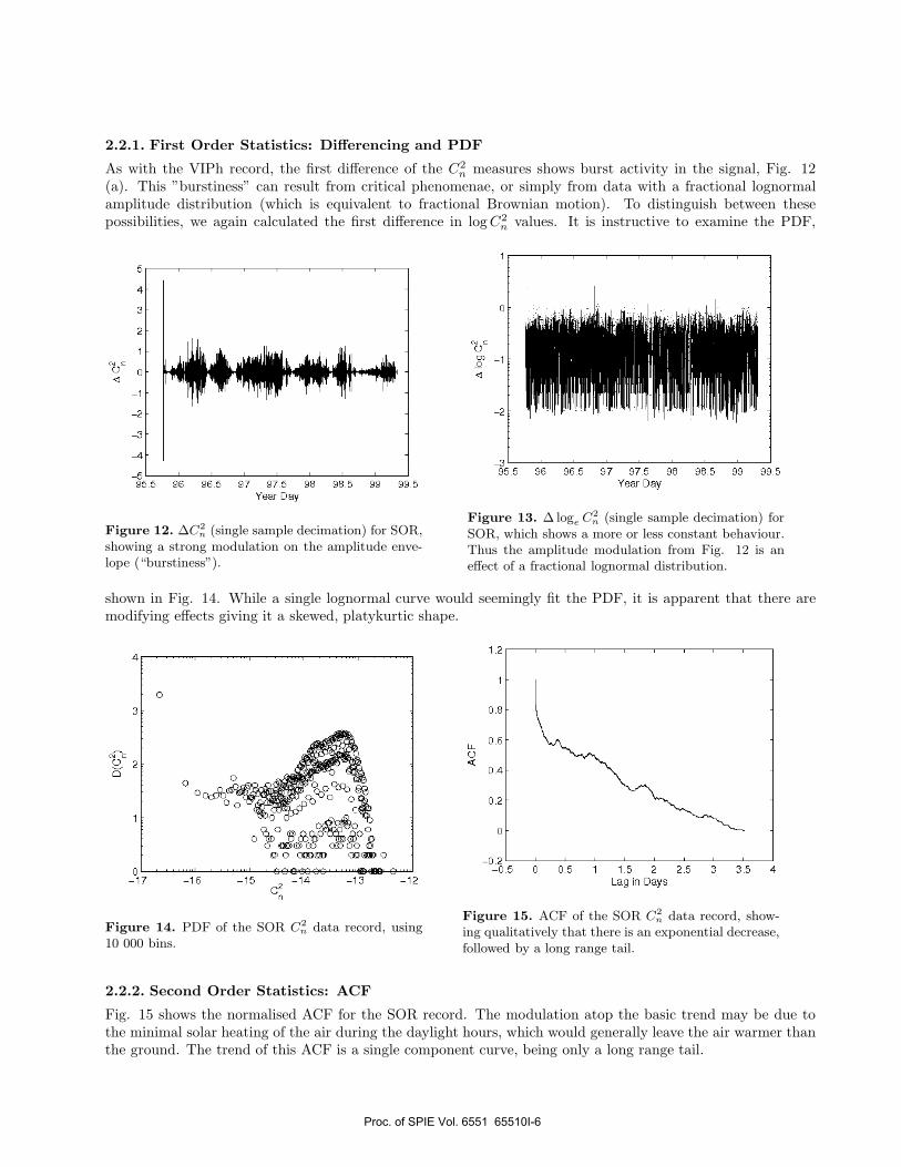
The probe beam was positioned at a mean height of 1 m above ground level at the receiver and transmitter ends,again aligned along a nearly North–South path of approximately 600 m length. The uneven intervening terraincaused beam altitude variations of up to 100 m along the path. Logistical considerations prevented a longer setfrom being obtained, although we fully intend to extend these data in the future. At first glance Figs. 10 and

Figure 10. The complete record of SOR measure-ments over 5 days.

Figure 11. The SOR data smoothed with a forwardrolling average of 120 points, which also includes thedata gaps.

11 show a lack of pronounced daytime ”bump” in the logarithmic SOR time series; this is a manifestation of thewell known temperature dependence of C2

n as temperatures were much lower than the VIPh environment. Thisis also evidenced in the lower mean value of C2

n. We observe that the minima are much more pronounced herethan for the VIPh record, though we cannot determine if this is a temporally local effect or it is more global inscope.


95.5 96 96.5 97 97.5 98 98.5 99 99.5Year Day

4

3

2

c_) 0•1

—l

—2

—3

-4955 96 965 97 975 98 985 99 995

Year Day

-16 -lb TT4C2

—13 —12

0

0 Oc0°& &Yo°a°0

o cE000 00 0 G& G' 0

LI-0.6

C)'C

0.4

0.2

—0.2—0.5 0 0.5 I 1.5 2 2.5 3 3.5 4

Lag in Days

2.2.1. First Order Statistics: Differencing and PDF

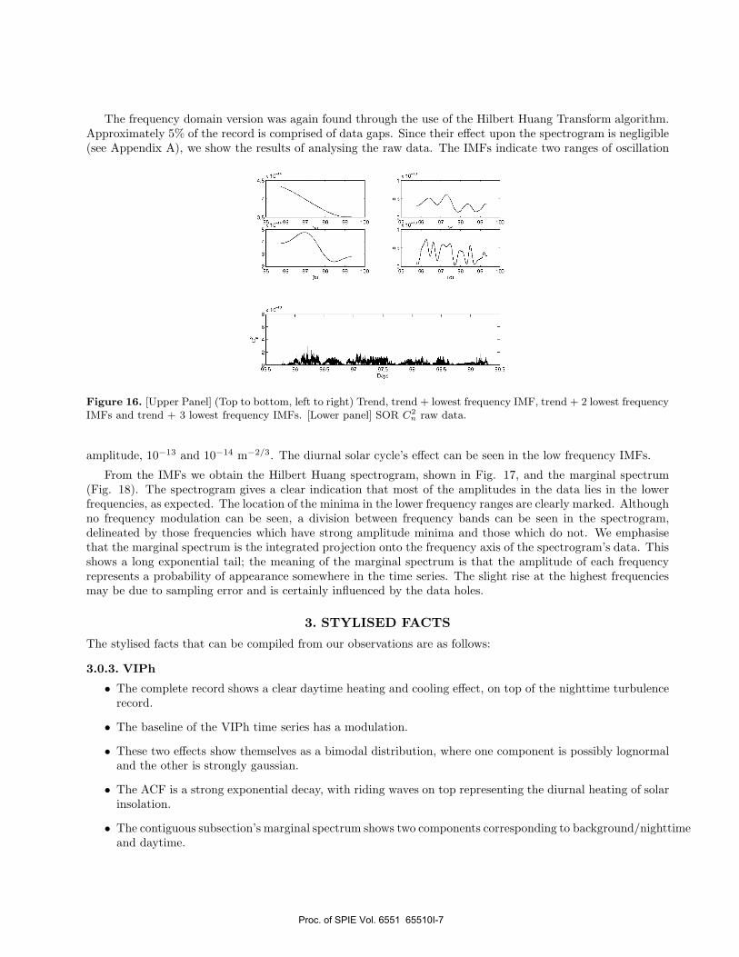
As with the VIPh record, the first difference of the C2n measures shows burst activity in the signal, Fig. 12

(a). This ”burstiness” can result from critical phenomenae, or simply from data with a fractional lognormalamplitude distribution (which is equivalent to fractional Brownian motion). To distinguish between thesepossibilities, we again calculated the first difference in log C2

n values. It is instructive to examine the PDF,

Figure 12. ∆C2n (single sample decimation) for SOR,

showing a strong modulation on the amplitude enve-lope (“burstiness”).

Figure 13. ∆ loge C2n (single sample decimation) for

SOR, which shows a more or less constant behaviour.Thus the amplitude modulation from Fig. 12 is aneffect of a fractional lognormal distribution.

shown in Fig. 14. While a single lognormal curve would seemingly fit the PDF, it is apparent that there aremodifying effects giving it a skewed, platykurtic shape.

Figure 14. PDF of the SOR C2n data record, using

10 000 bins.

Figure 15. ACF of the SOR C2n data record, show-

ing qualitatively that there is an exponential decrease,followed by a long range tail.

2.2.2. Second Order Statistics: ACF

Fig. 15 shows the normalised ACF for the SOR record. The modulation atop the basic trend may be due tothe minimal solar heating of the air during the daylight hours, which would generally leave the air warmer thanthe ground. The trend of this ACF is a single component curve, being only a long range tail.


7.5

55Q_s55 57 55 55 100

05 00 07 00 00 100

(b)

05.5 00 055 07 07.5 00 055 00 055Days

07 00 00 700

0.5

_05 00 07 00 00 700

(7)

The frequency domain version was again found through the use of the Hilbert Huang Transform algorithm.Approximately 5% of the record is comprised of data gaps. Since their effect upon the spectrogram is negligible(see Appendix A), we show the results of analysing the raw data. The IMFs indicate two ranges of oscillation

Figure 16. [Upper Panel] (Top to bottom, left to right) Trend, trend + lowest frequency IMF, trend + 2 lowest frequencyIMFs and trend + 3 lowest frequency IMFs. [Lower panel] SOR C2

n raw data.

amplitude, 10−13 and 10−14 m−2/3. The diurnal solar cycle’s effect can be seen in the low frequency IMFs.

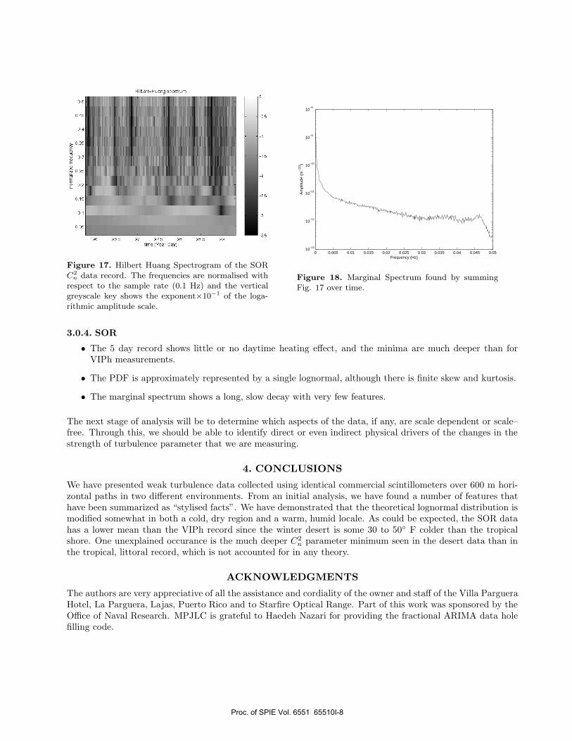
From the IMFs we obtain the Hilbert Huang spectrogram, shown in Fig. 17, and the marginal spectrum(Fig. 18). The spectrogram gives a clear indication that most of the amplitudes in the data lies in the lowerfrequencies, as expected. The location of the minima in the lower frequency ranges are clearly marked. Althoughno frequency modulation can be seen, a division between frequency bands can be seen in the spectrogram,delineated by those frequencies which have strong amplitude minima and those which do not. We emphasisethat the marginal spectrum is the integrated projection onto the frequency axis of the spectrogram’s data. Thisshows a long exponential tail; the meaning of the marginal spectrum is that the amplitude of each frequencyrepresents a probability of appearance somewhere in the time series. The slight rise at the highest frequenciesmay be due to sampling error and is certainly influenced by the data holes.

3. STYLISED FACTS

The stylised facts that can be compiled from our observations are as follows:

3.0.3. VIPh

• The complete record shows a clear daytime heating and cooling effect, on top of the nighttime turbulencerecord.

• The baseline of the VIPh time series has a modulation.

• These two effects show themselves as a bimodal distribution, where one component is possibly lognormaland the other is strongly gaussian.

• The ACF is a strong exponential decay, with riding waves on top representing the diurnal heating of solarinsolation.

• The contiguous subsection’s marginal spectrum shows two components corresponding to background/nighttimeand daytime.


Hilberr—Huang specrrum

SZS 98rime (Year Day)

Figure 17. Hilbert Huang Spectrogram of the SORC2

n data record. The frequencies are normalised withrespect to the sample rate (0.1 Hz) and the verticalgreyscale key shows the exponent×10−1 of the loga-rithmic amplitude scale.

0 0.005 0.01 0.015 0.02 0.025 0.03 0.035 0.04 0.045 0.0510

−13

10−12

10−11

10−10

10−9

10−8

Frequency (Hz)

Am

plitu

de (

m−

2/3 )

Figure 18. Marginal Spectrum found by summingFig. 17 over time.

3.0.4. SOR

• The 5 day record shows little or no daytime heating effect, and the minima are much deeper than forVIPh measurements.

• The PDF is approximately represented by a single lognormal, although there is finite skew and kurtosis.

• The marginal spectrum shows a long, slow decay with very few features.

The next stage of analysis will be to determine which aspects of the data, if any, are scale dependent or scale–free. Through this, we should be able to identify direct or even indirect physical drivers of the changes in thestrength of turbulence parameter that we are measuring.

4. CONCLUSIONS

We have presented weak turbulence data collected using identical commercial scintillometers over 600 m hori-zontal paths in two different environments. From an initial analysis, we have found a number of features thathave been summarized as “stylised facts”. We have demonstrated that the theoretical lognormal distribution ismodified somewhat in both a cold, dry region and a warm, humid locale. As could be expected, the SOR datahas a lower mean than the VIPh record since the winter desert is some 30 to 50◦ F colder than the tropicalshore. One unexplained occurance is the much deeper C2

n parameter minimum seen in the desert data than inthe tropical, littoral record, which is not accounted for in any theory.

ACKNOWLEDGMENTS

The authors are very appreciative of all the assistance and cordiality of the owner and staff of the Villa PargueraHotel, La Parguera, Lajas, Puerto Rico and to Starfire Optical Range. Part of this work was sponsored by theOffice of Naval Research. MPJLC is grateful to Haedeh Nazari for providing the fractional ARIMA data holefilling code.


APPENDIX A.

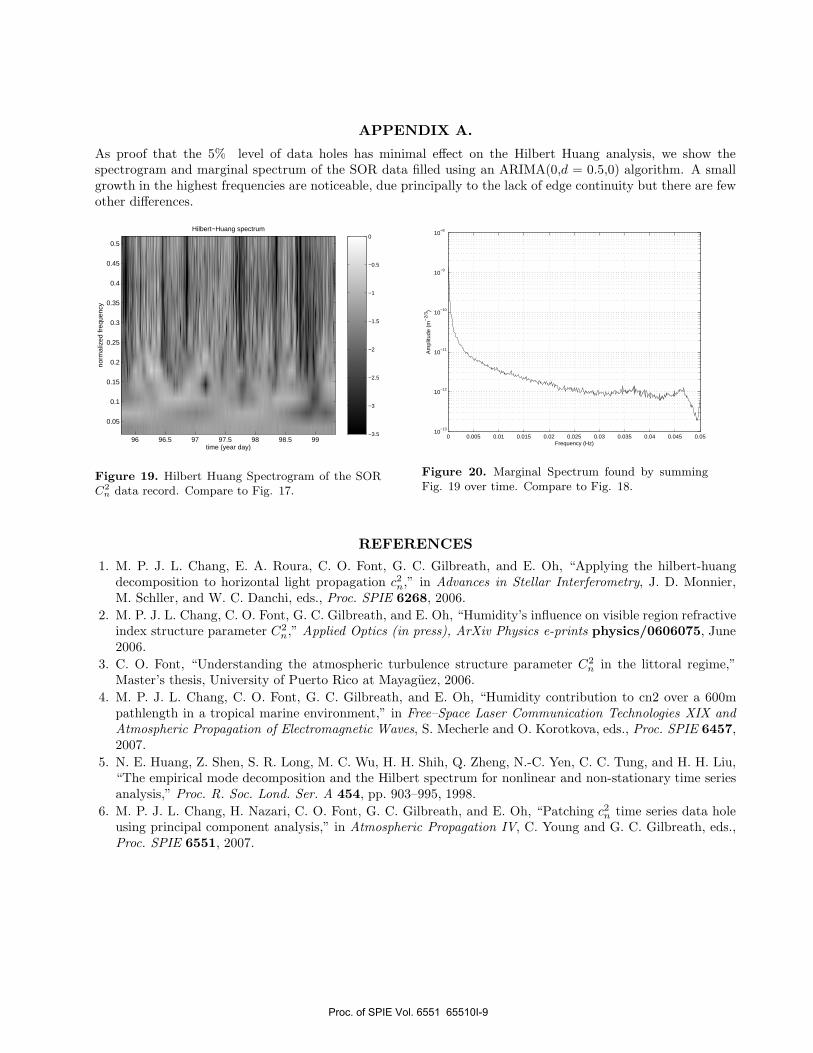
As proof that the 5% level of data holes has minimal effect on the Hilbert Huang analysis, we show thespectrogram and marginal spectrum of the SOR data filled using an ARIMA(0,d = 0.5,0) algorithm. A smallgrowth in the highest frequencies are noticeable, due principally to the lack of edge continuity but there are fewother differences.

time (year day)

norm

aliz

ed fr

eque

ncy

Hilbert−Huang spectrum

96 96.5 97 97.5 98 98.5 99

0.05

0.1

0.15

0.2

0.25

0.3

0.35

0.4

0.45

0.5

−3.5

−3

−2.5

−2

−1.5

−1

−0.5

0

Figure 19. Hilbert Huang Spectrogram of the SORC2

n data record. Compare to Fig. 17.

0 0.005 0.01 0.015 0.02 0.025 0.03 0.035 0.04 0.045 0.0510

−13

10−12

10−11

10−10

10−9

10−8

Frequency (Hz)

Am

plitu

de (

m−

2/3 )

Figure 20. Marginal Spectrum found by summingFig. 19 over time. Compare to Fig. 18.

REFERENCES1. M. P. J. L. Chang, E. A. Roura, C. O. Font, G. C. Gilbreath, and E. Oh, “Applying the hilbert-huang

decomposition to horizontal light propagation c2n,” in Advances in Stellar Interferometry, J. D. Monnier,

M. Schller, and W. C. Danchi, eds., Proc. SPIE 6268, 2006.2. M. P. J. L. Chang, C. O. Font, G. C. Gilbreath, and E. Oh, “Humidity’s influence on visible region refractive

index structure parameter C2n,” Applied Optics (in press), ArXiv Physics e-prints physics/0606075, June

2006.3. C. O. Font, “Understanding the atmospheric turbulence structure parameter C2

n in the littoral regime,”Master’s thesis, University of Puerto Rico at Mayaguez, 2006.

4. M. P. J. L. Chang, C. O. Font, G. C. Gilbreath, and E. Oh, “Humidity contribution to cn2 over a 600mpathlength in a tropical marine environment,” in Free–Space Laser Communication Technologies XIX andAtmospheric Propagation of Electromagnetic Waves, S. Mecherle and O. Korotkova, eds., Proc. SPIE 6457,2007.

5. N. E. Huang, Z. Shen, S. R. Long, M. C. Wu, H. H. Shih, Q. Zheng, N.-C. Yen, C. C. Tung, and H. H. Liu,“The empirical mode decomposition and the Hilbert spectrum for nonlinear and non-stationary time seriesanalysis,” Proc. R. Soc. Lond. Ser. A 454, pp. 903–995, 1998.

6. M. P. J. L. Chang, H. Nazari, C. O. Font, G. C. Gilbreath, and E. Oh, “Patching c2n time series data hole

using principal component analysis,” in Atmospheric Propagation IV, C. Young and G. C. Gilbreath, eds.,Proc. SPIE 6551, 2007.


Comparing horizontal path C n measurements over 0.6 ... - DTIC

Documents