Comparing evolutionary rates for different phenotypic traits on a phylogeny using likelihood

[11:15 30/1/2013 Sysbio-sys083.tex] Page: 181 181–192

Syst. Biol. 62(2):181–192, 2013© The Author(s) 2012. Published by Oxford University Press, on behalf of the Society of Systematic Biologists. All rights reserved.For Permissions, please email: [email protected]:10.1093/sysbio/sys083Advance Access publication September 27, 2012

Comparing Evolutionary Rates for Different Phenotypic Traits on a Phylogeny UsingLikelihood

DEAN C. ADAMS∗

Department of Ecology, Evolution, and Organismal Biology and Department of Statistics, Iowa State University, Ames, IA 50011, USA∗Correspondence to be sent to: E-mail: [email protected].

Received 31 May 2012; reviews returned 14 August 2012; accepted 17 September 2012Associate Editor: Luke Harmon

Abstract.—In recent years, likelihood-based approaches have been used with increasing frequency to evaluatemacroevolutionary hypotheses of phenotypic evolution under distinct evolutionary processes in a phylogenetic context(e.g., Brownian motion, Ornstein-Uhlenbeck, etc.), and to compare one or more evolutionary rates for the same phenotypictrait along a phylogeny. It is also of interest to determine whether one trait evolves at a faster rate than another trait. However,to date no study has compared phylogenetic evolutionary rates between traits using likelihood, because a formal approachhas not yet been proposed. In this article, I describe a new likelihood procedure for comparing evolutionary rates for two ormore phenotypic traits on a phylogeny. This approach compares the likelihood of a model where each trait evolves at a distinctevolutionary rate to the likelihood of a model where all traits are constrained to evolve at a common evolutionary rate. Themethod can also account for within-species measurement error and within-species trait covariation if available. Simulationsrevealed that the method has appropriate Type I error rates and statistical power. Importantly, when compared with existingapproaches based on phylogenetically independent contrasts and methods that compare confidence intervals for modelparameters, the likelihood method displays preferable statistical properties for a wide range of simulated conditions. Thus,this likelihood-based method extends the phylogenetic comparative biology toolkit and provides evolutionary biologistswith a more powerful means of determining when evolutionary rates differ between phenotypic traits. Finally, I providean empirical example illustrating the approach by comparing rates of evolution for several phenotypic traits in Plethodonsalamanders. [Evolutionary rates; macroevolution; morphological evolution; phenotype; phylogenetic comparative method;phylogeny.]

Describing the pace of evolutionary change isessential for understanding how morphological,and ultimately, biological diversity is generatedand maintained. Biologists have often observedthat rates of phenotypic evolution differ acrosstaxonomic groups (e.g., Simpson 1944; Gingerich 1993;Harmon et al. 2003; Hulsey et al. 2010). Furthermore,differences or changes in evolutionary rates may playa significant role generating large-scale phenotypictrends (Foote 1997; Sidlauskas 2008; Ackerly 2009).Indeed, several evolutionary models posit a direct linkbetween contemporary selection pressures, rates ofphenotypic evolution, and macroevolutionary patternsof phenotypic diversification (see Hansen and Martins1996; Schluter 2000; Mahler et al. 2010). However, testingthese hypotheses has remained a challenge, in partbecause methods for assessing rates of phenotypicevolution in a phylogenetic context have only recentlybeen developed (e.g., Garland 1992; O’Meara et al. 2006;Thomas et al. 2006).

Frequently, evolutionary rates are quantified in termsof the amount of phenotypic change between ancestorand descendent lineages, standardized by time. Oneapproach, the “darwin” (Haldane 1949), measuresevolutionary rates in terms of the difference of log-trait values between ancestors and descendents permillion years, and is often used in paleontologicalstudies. Another measure, the “haldane” (Gingerich1983), estimates the evolutionary rate as the change inphenotypic trait values across generations (standardizedfor variation within traits) and is more commonly usedin neontological studies. For sets of traits, Mahalanobis

distance has been used as a multivariate analog of thehaldane (Lerman 1965; Gingerich 2009; Arnegard etal. 2010), although this has sometimes been applied topairs of extant species rather than ancestor–descendentlineages (e.g., Arnegard et al. 2010; Carlson et al. 2011).Both darwins and haldanes have been used extensivelyto estimate the pace of evolutionary change in a widevariety of taxa and traits (for reviews, see Gingerich1983, 1993, 2009; Hendry and Kinnison 1999; Hendry etal. 2008). However, a shortcoming of these measures isthat they only estimate evolutionary rates between pairsof taxa. When the rate of phenotypic evolution for anentire clade of organisms is of interest, methods thatincorporate the phylogenetic relatedness among taxa arerequired.

Over the past several years, likelihood-basedapproaches have been developed for estimatingthe rate of phenotypic change along a phylogenybased on a particular model of evolution. Typically, aBrownian motion (BM) model of evolution is utilized(Edwards and Cavalli-Sforza 1964; Felsenstein 1973,1985), although other models describing alternativescenarios of phenotypic evolution, such as Ornstein-Uhlenbeck (OU: Lande 1976; Hansen and Martins 1996;Hansen 1997; Butler and King 2004) and early-burst (EB)models (Blomberg et al. 2003), can also be examined.In addition, evolutionary models that include distinctevolutionary rates on different parts of the phylogenycan be assessed. Here, likelihood approaches are usedto compare the fit of an evolutionary model with asingle rate to a model containing multiple evolutionaryrates (e.g., O’Meara et al. 2006; Thomas et al. 2006) to

181

at Iowa State U

niversity on February 15, 2013http://sysbio.oxfordjournals.org/

Dow

nloaded from

http://sysbio.oxfordjournals.org/


182 SYSTEMATIC BIOLOGY VOL. 62

determine whether the tempo of phenotypic evolutionhas changed on particular branches of the phylogeny(see also Eastman et al. 2011; Revell et al. 2012). Suchapproaches can provide evidence for differencesin evolutionary rates among clades, or shifts inevolutionary rates within clades (e.g., Collar et al. 2009;Thomas et al. 2009; Hulsey et al. 2010). An increasingnumber of studies have used this approach to examinethe tempo of evolution in various phenotypic traitswithin and among lineages (e.g., Collar et al. 2009;Thomas et al. 2009; Harmon et al. 2010; Mahler et al.2010; Price et al. 2010; Valenzuela and Adams 2011).

Another important question concerning the tempoof evolution is whether one phenotypic trait evolvesat a faster rate than another. Numerous studies haveexamined trait evolution in both fossil and extantlineages, revealing considerable variation in the rateof phenotypic evolution among traits and clades(Gingerich 1983, 1993; Hendry and Kinnison 1999;Hunt 2007; Ackerly 2009). Furthermore, several authorshave suggested that some phenotypic traits, such asbehavioral characteristics, evolve at a faster rate thanother traits, such as morphology (Huey and Bennett1987; Gittleman et al. 1996; Blomberg et al. 2003). Indeed,comparisons of phylogenetically independent contrastsfor different traits have revealed that some traits doevolve faster than others (Garland 1992; Katzourakis et al.2001; Hone et al. 2005; Ackerly 2009), lending support tothis hypothesis. In addition, several recent studies havequantified evolutionary rates for multiple traits usinglikelihood approaches (Adams et al. 2009; Revell andCollar 2009; Harmon et al. 2010; Martin and Wainwright2011). Thus, at first glance it appears conceptuallystraightforward to employ likelihood approaches toidentify differences in evolutionary rates among traits.However, no study has explicitly compared evolutionaryrates between traits in a phylogenetic framework usinglikelihood, because methods have not been developedfor testing the hypothesis that different traits evolveat distinct evolutionary rates. In this article, I extendexisting methods by describing a likelihood procedurethat allows the comparison of evolutionary rates fortwo or more phenotypic traits on a phylogeny. Withthe approach, within-species measurement error andwithin-species trait covariation can also be accounted forwhen these are available. I then compare the statisticalperformance of this method to several alternativeapproaches, and show that the likelihood approach haspreferable statistical properties. I provide a biologicalexample demonstrating the utility of the approach,and computer code written in R for implementing theprocedure.

COMPARING EVOLUTIONARY RATES FOR

DIFFERENT TRAITS

For a single phenotypic trait, the evolutionary rateof change under a BM model of evolution can beestimated using several analytical approaches, such as

phylogenetic generalized least squares (PGLS: Grafen1989; Martins and Hansen 1997), independent contrasts(e.g., Garland and Ives 2000), and maximum likelihood(e.g., O’Meara et al. 2006). Using the PGLS formulation,the least squares and maximum likelihood estimates(MLE) of the evolutionary rate parameter are equivalent(Felsenstein 1973; see also Garland and Ives 2000;O’Meara et al. 2006), and can be found as:

�2 =[Y−E

(Y

)]t C−1[Y−E

(Y

)]N

(1)

where Y is a N × 1 column vector containing thephenotypic values for the N species, and E(Y) is aN × 1 column vector of phylogenetic means, foundas a=(

1tC−11)−1(

1tC−1Y)

(Rohlf 2001; Blomberg et al.2003; O’Meara et al. 2006) [note: matrix notation isretained here for consistency with previous authors(e.g., O’Meara et al. 2006), and because Y could alsorepresent a matrix of phenotypic values, in which case,a would be a vector, see Revell and Collar 2009]. Thephylogenetic relationships among taxa are encoded bythe phylogenetic covariance matrix, C, which is an N × Nmatrix constructed from the phylogenetic tree (Garlandand Ives 2000; Freckleton et al. 2002; O’Meara et al. 2006;Thomas et al. 2006). Notice that equation (1) representsthe MLE of �2, which is slightly downwardly biased (seeO’Meara et al. 2006). To obtain the unbiased estimate of�2, the numerator of equation (1) is divided by (N−1)rather than N. A numerically equivalent estimate of �2

can also be obtained using phylogenetically independentcontrasts rather than PGLS (see e.g., Felsenstein 1985;Garland 1992; Garland and Ives 2000; Ackerly 2009).Finally, for a univariate trait and under a BM modelof evolution, the log likelihood of �2, given thephenotypic data (Y), the ancestral state (a), and thephylogeny (C) is derived from the multivariate normaldistribution (Felsenstein 1973; O’Meara et al. 2006),and is given by:

log(L)=− 1

2

{[Y−E

(Y

)]t(�2C

)−1[Y−E

(Y

)]}

−log∣∣∣�2C

∣∣∣/2−N log(2�)/2. (2)

For a set of traits treated simultaneously (i.e., amultivariate Y matrix), equation (1) results in anevolutionary rate matrix (R: sensu Revell and Harmon2008), which is the algebraic extension of �2 (Freckletonet al. 2002; McPeek et al. 2008; Revell and Harmon2008; Adams et al. 2009). Here, the diagonal elements(�2

ii) represent the evolutionary rates for each of theindividual traits and are identical to the evolutionaryrates estimated for each trait when it is analyzedseparately. The off-diagonal elements (�2

ij) describe theevolutionary covariation between traits, which havebeen interpreted as evolutionary correlations betweencharacters (e.g., Revell and Collar 2009). Under a BMmodel of evolution, the log likelihood of R, given the

at Iowa State U


Dow

nloaded from



2013 ADAMS—COMPARING EVOLUTIONARY RATES AMONG TRAITS 183

phenotypic data (Y), the ancestral state for each of thetraits (a), and the phylogeny (C) is obtained from ageneralization of equation (2):

log(L)=− 1

2

{[Y−E

(Y

)]t (R⊗C)−1[

Y−E(Y

)]}−log|R⊗C|/2−N log(2�)/2 (3)

where the expected evolutionary covariance matrix isfound as the Kronecker product of the evolutionary ratematrix and the phylogenetic covariance matrix (R⊗C=V, see Revell and Harmon 2008).

To determine whether two or more phenotypic traitsdiffer in their evolutionary rates, one can comparethe log likelihoods from two alternative models thatdescribe distinct ways in which phenotypic variationevolves. In the first model, each trait evolves accordingto its own evolutionary rate, whereas in the secondmodel, all phenotypic traits are constrained to evolveat a common evolutionary rate. This procedure isconceptually similar to methods that evaluate changesin evolutionary rates for a single trait on a phylogenyby comparing a model containing one rate to modelscontaining two or more rates in different parts of thetree (e.g., O’Meara et al. 2006; Thomas et al. 2006;Revell 2008; Revell and Harmon 2008; Thomas et al.2009). For the model where all traits evolve at theirown separate rates, the evolutionary rate matrix (R) forall traits is obtained using equation (1), and the loglikelihood of this evolutionary model is found usingequation (3). Next, the alternative evolutionary scenariois examined, where all phenotypic traits are constrainedto evolve at a common rate. For this model, there isa common evolutionary rate along the diagonal of theevolutionary rate matrix (R), but all trait covariancesare left unconstrained. Determining the log likelihood ofthis alternative model requires an optimization routinethat searches over possible rate matrices containing acommon evolutionary rate �2, and selects the rate matrixR that maximizes the joint likelihood for the traits asdescribed in equation (3). Unfortunately, implementingthis procedure is not straightforward due to a numberof computational issues. First, the rate matrix must bepositive semidefinite, as R is a covariance matrix. Thiscriterion can be satisfied by optimizing over parametersof the Cholesky decomposition of R, rather than therates and evolutionary covariances that comprise therate matrix itself (see Revell and Collar 2009; Revell2012). Second, the optimization is further complicatedby the fact that the rate matrix R must be constrainedto have equal values along its diagonals. Typically,parameters from matrix decomposition do not guaranteethis property. However, this mathematical constraintmay be imposed in the Cholesky decomposition of Rby adjusting the manner in which the Cholesky matrixis derived. Appendix 1 provides the algebraic detailsfor obtaining this constrained Cholesky decomposition,which is utilized here.

Using parameters from the constrained Choleskydecomposition, likelihood optimization may proceed

in the usual fashion. First, an initial set of parametersare provided, and used to generate the rate matrixR, which, by construction, is constrained to containequal diagonal elements. The likelihood of this modelis then found using equation (3). Next a quasi-Newtonmethod is used to search an approximation of thelog likelihood surface to identify the parameters thatmaximize the log likelihood as described in equation(3). This approach thus identifies the MLE foundunder the constraint that the diagonal elements ofthe rate matrix R are equal. The two evolutionarymodels are then statistically compared using a likelihoodratio test

[LRT=−2

(logLconstrained −logLobs

)], which is

approximately chi-square distributed with p−1 degreesof freedom (the difference in estimated parametersbetween the observed and constrained models). Asignificant LRT provides support for the hypothesisthat the phenotypic traits evolve at different rates.Additionally, AIC values can be obtained and comparedfor the two models. Computer code written in Rfor implementing the above procedures is found inAppendix 2.

Finally, an alternative implementation of the aboveprocedure may be used to model the scenario where noevolutionary covariation between traits is assumed. Thisis accomplished by setting the off-diagonal elements ofthe rate matrix to zero and maximizing the likelihoodof this model, which is identical to the sum of thelog likelihoods for each trait treated separately (resultsnot shown). In this case, the alternative model ofequal rates for all traits is optimized for the commonevolutionary rate �2, and the value of �2 that maximizesthe joint likelihood for the traits as described in equation(3) is treated as the common evolutionary rate forall traits. Note that although models assuming traitindependence are biologically unrealistic (as phenotypictraits are frequently evolutionarily correlated), thisapproach is analogous to rate comparisons based onphylogenetically independent contrasts (Garland 1992),which are obtained for each trait individually andwithout incorporating evolutionary covariation betweentraits.

Trait ScaleOne important consideration when comparing

evolutionary rates among traits is the effect of traitscale. Trait variation is dependent on both units andscale, with larger traits generally displaying largervariances (Sokal and Rohlf 2011). Evolutionary rates(which are phylogenetically standardized variances)are also scale-dependent (Gingerich 1993; Arnegard etal. 2010); for instance, a trait represented in millimeterswill have a �2 that is 100 times higher than �2 for thesame data represented in centimeters. Similarly, traitsthat differ greatly in their means will have differentper-unit changes, because traits with larger valuesare expected to have larger changes per unit time.As a consequence, comparisons of evolutionary rates

at Iowa State U


Dow

nloaded from




between traits may be compromised if the traits underinvestigation are not in commensurate units. A numberof authors have advocated log-transforming the dataprior to the estimate of evolutionary rates (Felsenstein1985; O’Meara et al. 2006; Ackerly 2009; Gingerich 2009).This provides a scale-free estimate of evolutionaryrates, and has the desirable property that evolutionaryrates are described as the relative rate of change inproportion to the mean for each trait. Furthermore,log-transformation permits the comparison of traitsmeasured in different units, because the resultingevolutionary rates are expressed in terms of the relativechange in proportion to the mean for each trait. In accordwith these suggestions, I recommend that when traits arein different scales, they should be log-transformed priorto the comparison of evolutionary rates. However, forinstances, when scale dependence cannot be accountedfor by log-transformation, alternative transformationsmay be required.

Within-Species Variation and Measurement ErrorAnother important consideration when comparing

evolutionary rates is measurement error. Mostphylogenetic comparative studies assume that within-species variation is negligible. However, within-speciesvariation and measurement error can have a profoundeffect on parameters estimated from evolutionarymodels (Ives et al. 2007; Felsenstein 2008). For instance,increased within-species variation (or sampling error)will cause evolutionary rates to be overestimated(Ives et al. 2007). This can complicate comparisonsof evolutionary rates between traits, as differences insampling error can lead to perceived differences inevolutionary rates. Several methods for incorporatingwithin-species variation in phylogenetic comparativeanalyses have recently been proposed (Ives et al. 2007;Felsenstein 2008; also O’Meara et al. 2006; Harmon et al.2010). For instance, for a single trait, the within-speciesmeasurement error can be accounted for by adding thisvariation to the diagonal of the expected evolutionarycovariance matrix (V) before calculating the likelihood(Harmon et al. 2010; also O’Meara et al. 2006). In thiscase, however, V is of dimension

(pN×pN

), as it is found

through the Kronecker product of the evolutionaryrate matrix and the phylogenetic covariance matrix(R⊗C=V). Therefore, a generalization of the approachdescribed earlier is utilized. Here, the within-speciesmeasurement error vectors for each trait are firstconcatenated into a vector of length pN. This vector isthen added to the diagonal of V prior to the likelihoodcalculations. Additionally, if within-species traitcovariation is available, this can also be incorporatedby adding it to the appropriate subdiagonals of V (i.e.,those elements of V that represent the trait covariationwithin each species for each pair of traits). The approachallowing for within-species measurement error andwithin-species trait covariation is implemented in thecomputer code in Appendix 2.

Additional Tests and Flow of ComputationsWith all analytical approaches, sound biological

inferences are only possible when alternativeexplanations for the observed patterns have beeninvestigated. In this regard, several alternativesshould be considered when testing for differencesin evolutionary rates. First, perceived differencesin evolutionary rates may arise simply because thephenotypic traits are in different scales; as largertraits are expected to have higher rates (see above). Assuch, log transforming the data prior to the estimateof evolutionary rates is recommended for traits thatdiffer notably in scale. Second, measurement errormay generate perceived differences in evolutionaryrates, so when possible, within-species measurementerror should be examined and accounted for (seeabove). Finally, comparisons of evolutionary rates maybe compromised if the traits differ in their degree ofphylogenetic structure (Blomberg et al. 2003), or if theirpatterns of diversification follow distinct models ofevolution (e.g., BM vs. EB). As distinct modes of traitevolution are possible, it is recommended that model-fitting procedures first be used to determine whethera BM model of evolution best describes the observedpatterns of phenotypic diversification for the set of traits,or whether some alternative model is favored. However,it should also be noted that while such proceduresallow the best fitting model to be identified, BM stillprovides a general overall measure of the evolutionaryrate of change of a trait along the phylogeny, and thusremains useful for identifying traits that differ greatlyin their evolutionary rates. In other words, �2 representsthe “effective rate” of trait evolution (see discussion inAckerly 2009), although when models differ markedlybetween traits, comparisons of �2 must be evaluatedmore cautiously.

STATISTICAL PERFORMANCE

To evaluate the performance of the proposedlikelihood procedure, I executed a series of computersimulations. For each simulation, 1000 randomphylogenies containing 32 taxa were generated(results from a wider set of phylogenies underdifferent conditions are found in the SupplementalMaterial, available on Dryad at http://datadryad.org,doi:10.5061/dryad.1117q). Two continuous phenotypictraits were then evolved along each phylogeny under avariety of conditions. Changes in both traits followed aBM model of evolution, with a rate parameter for thefirst trait of �2

1 =1.0, and the rate of the second traitequal to or exceeding that of the first trait, dependingupon simulation conditions. Evolutionary rates for bothtraits were then estimated as described earlier, and alikelihood ratio test was used to determine whetheror not the traits differed in their evolutionary rates(both implementations of the likelihood approachwere evaluated: Supplemental Material). Additionally,

at Iowa State U


Dow

nloaded from




two alternative approaches were used to test fordifferences in evolutionary rates. First, phylogeneticallyindependent contrasts were obtained for each trait, andevolutionary rates for the two traits were comparedusing a t-test on the absolute value of the contrasts(Garland 1992). Second, 95% confidence intervals(CIs) were estimated from the standard errors of eachevolutionary rate as obtained from the Hessian matrix,and these CIs were examined for potential overlap (fordetails, see Supplemental Material). For all approaches,the number of significant results (out of 1000) wastreated as an estimate of Type I error (when �2

1 =�22)

or statistical power (when �22/�

21 >1.0). Results from

additional computer simulations for a wider range ofconditions are found in the Supplemental Material.

Using this procedure, I found that the likelihood-based approach displayed appropriate Type I error rates,and its statistical power increased rapidly as the relativedifference in evolutionary rates between traits increased(Fig. 1). Furthermore, the likelihood-based approachdisplayed higher statistical power than the method basedon independent contrasts (Fig. 1), and this result wasconsistent across all simulation conditions evaluated(Supplemental Figures 1 and 2). Similarly, the likelihood-based approach outperformed the method based on 95%CI. Here, the latter displayed Type I error rates lowerthan expected, and had low power when differencesbetween evolutionary rates were small (Fig. 1). Finally,simulations revealed that the method performed equallywell when traits were simulated with or withoutevolutionary covariation between them (SupplementalFigure 3), and parameter estimates obtained fromthe likelihood approach adequately represented inputrates for the simulations (Supplemental Figure 4).Overall, these results demonstrate that the likelihood-based method exhibits superior statistical propertiesas compared with alternative approaches, and thusprovides a powerful means of detecting differences inevolutionary rates between traits. This represents animportant analytic advance over existing approaches.

A BIOLOGICAL EXAMPLE

To illustrate the methods described earlier, I provide abiological example comparing evolutionary rates amongmultiple phenotypic traits in Plethodon salamanders.Plethodon are long-lived, direct-developing terrestrialsalamanders found in North American forests (Highton1995). Forty-five species inhabit eastern North America,and extensive field collecting at thousands of geographiclocalities has rigorously documented their geographicdistributions. Considerable behavioral and ecologicalresearch has shown that interspecific competition iswidespread (e.g., Jaeger 1971; Hairston 1980; Anthonyet al. 1997; Deitloff et al. 2008), and likely influencescommunity structure at both a local and regional scale(Adams 2007). In Plethodon, interspecific competition isoften mediated through aggressive encounters, in whichagonistic displays (e.g., all-trunk raised: Jaeger and

FIGURE 1. Statistical power curves for tests to compare rates ofevolution revealed by computer simulations based on a phylogenycontaining 32 taxa. The abscissa shows the relative difference inevolutionary rates between the 2 traits, whereas the ordinate displaysthe relative power based on the percentage of 1000 simulations found tobe significant. Results for the likelihood-based approach are shown asblack dots, results for the independent contrasts approach are shownas gray squares, and results from a comparison of 95% CIs of modelparameter are shown as white diamonds. Results from simulationsconduced over a wider set of conditions are found in the SupplementalMaterial.

Forester 1993) and biting (Anthony et al. 1997) frequentlydetermine which individual is competitively superior. Insome instances, interspecific competition has resulted inthe evolution of morphological differences, particularlyin head shape (e.g., Adams 2000, 2004, 2010; Adams andRohlf 2000; Adams et al. 2007; Arif et al. 2007). Further,body size differences are prevalent between species(Adams and Church 2008, 2011), and because Plethodonare generalist predators (Petranka 1998), species ofsimilar size may compete more intensively for similarprey resources (see Kozak et al. 2009). Together, theseobservations suggest the hypothesis that morphologicaltraits associated with species interactions, such asaggressive encounters or differential food acquisition,may have elevated rates of evolution as compared withother phenotypic attributes.

I obtained linear measurements for three phenotypictraits (head length, forelimb length, and body width)from 311 adult individuals, representing 44 of the 45species of eastern Plethodon (Fig. 2a; data from Adamset al. 2009). For these traits, head length is expected tobe related to competitive interactions between species,as an increased head length is correlated with increasedjaw length, which in turn is related to both aggressivebiting and prey acquisition (see e.g., Maglia and Pyles1995; Adams and Rohlf 2000). Similarly, forelimb lengthis expected to be related to competitive interactions, asgreater forelimb length results in greater perceived bodysize during aggressive displays (Jaeger and Forester

at Iowa State U


Dow

nloaded from




FIGURE 2. a) Locations of 3 linear measurements obtained fromadult Plethodon salamanders (HL, head length; FL, forelimb length;BW, body width). b) Estimates of evolutionary rates for 3 linear traitsused in this study, with their 95% CIs.

1993). For these species body width has no knownassociation with selection mediated through competitiveinteractions. For each species, the mean value of eachtrait was obtained, and because all the 3 traits weremeasured in the same units (mm) and of the same scale(similar means and ranges), untransformed values wereused for all analyses. AIC comparisons of evolutionarymodels (BM, OU, and EB) revealed that a BM model wasthe best model (i.e., lowest AIC) for 2 of the 3 phenotypictraits (forelimb length and body width), and had a �AIC<4.0 from the best model for head length. As such, a BMmodel was used in all subsequent analyses (see Burnhamand Anderson 2002, p. 70).

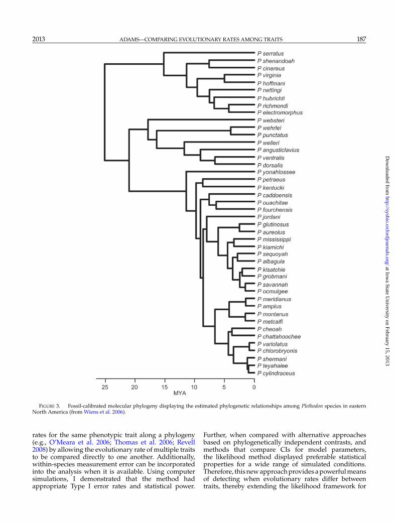
From the species means I estimated the rate ofevolution for each trait under a BM model of evolution(�2) using a multigene, time-calibrated molecularphylogeny (Wiens et al. 2006) for the genus (Fig. 3).Rate assessments were performed on both the set ofmean trait values as described here, as well as the setof mean trait values standardized by the mean bodysize for each species. To determine whether or not thephenotypic traits evolved at similar rates, I used theprocedure described earlier by comparing evolutionaryrates among traits while allowing for evolutionarycovariation between traits. In addition, analyses wereperformed for all pairs of traits to determine whichmorphological traits evolved at different rates. Becauseestimates of within-species variation and within-speciestrait covariation were available, I repeated the primaryanalysis above while accounting for measurement errorin the likelihood calculations. Finally, for comparison, Iexamined the evolutionary rates among the traits under

the model where no evolutionary covariation betweentraits was included. All calculations were performedin R 2.15 (R Development Core Team 2012) using theAPE library (Paradis et al. 2004; Paradis 2012) and newroutines written by the author (Appendix 2).

RESULTS

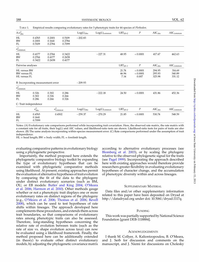
Likelihood ratio tests indicated that the threemorphological traits were not evolving at a commonevolutionary rate (Fig. 2b; Table 1). Further, pairwisecomparisons revealed that both head length andforelimb length displayed considerably higherevolutionary rates than did body width, but theevolutionary rates for head length and forelimb lengthwere not distinguishable from one another (Table 1).Analyses of traits standardized for body size yieldedsimilar results to those described above (results notshown). AIC results were consistent with results foundusing likelihood, and showed that head length andforelimb length did not have appreciably distinctevolutionary rates, as the preferred model for thiscomparison was one with a single evolutionary rate forthe two traits (Table 1). Incorporating within-speciesmeasurement error did not alter the results describedabove, as the likelihood ratio test under this scenarioalso revealed differences in evolutionary rates amongthe traits (Table 1). Similarly, analyses incorporatingwithin-species trait covariation yielded consistentresults with those reported here (not shown). Finally,for this example, statistical results obtained from amodel assuming no evolutionary covariation betweentraits were concordant with results obtained froma model where evolutionary trait covariation wasincorporated (Table 1). Therefore, biological conclusionsfrom both approaches were equivalent. As expected, themodel incorporating trait covariation had considerablybetter AIC and likelihood scores as compared to themodel with no trait covariation, indicating that itprovided a better description of phenotypic variationand evolutionary change in these phenotypic traits(Table 1). Biologically, the results here suggest thatin Plethodon, different morphological traits evolveat distinct evolutionary rates. Further, because headlength and forelimb length are related to competitiveinteractions, these observations are consistent with thehypothesis that selection resulting from interspecificinteractions may increase the evolutionary rate of thosetraits important for such encounters, which may furtherenhance the morphological diversification in Plethodon(see discussion in Adams 2011).

DISCUSSION

In this article, I described an approach for comparingevolutionary rates for two or more phenotypic traitsusing likelihood. The approach extends existingprocedures for comparing one or more evolutionary

at Iowa State U


Dow

nloaded from




FIGURE 3. Fossil-calibrated molecular phylogeny displaying the estimated phylogenetic relationships among Plethodon species in easternNorth America (from Wiens et al. 2006).

rates for the same phenotypic trait along a phylogeny(e.g., O’Meara et al. 2006; Thomas et al. 2006; Revell2008) by allowing the evolutionary rate of multiple traitsto be compared directly to one another. Additionally,within-species measurement error can be incorporatedinto the analysis when it is available. Using computersimulations, I demonstrated that the method hadappropriate Type I error rates and statistical power.

Further, when compared with alternative approachesbased on phylogenetically independent contrasts, andmethods that compare CIs for model parameters,the likelihood method displayed preferable statisticalproperties for a wide range of simulated conditions.Therefore, this new approach provides a powerful meansof detecting when evolutionary rates differ betweentraits, thereby extending the likelihood framework for

at Iowa State U


Dow

nloaded from




TABLE 1. Empirical results comparing evolutionary rates for 3 phenotypic traits for 44 species of Plethodon.

A:�2obs Log(L)obs Log(L)common LRTdf=2 P AICobs AICcommon

HL 0.4765 0.2001 0.5109 −202.83BW 0.2001 0.1641 0.2784FL 0.5109 0.2784 0.7099

�2common

HL 0.4177 0.2744 0.3422 −227.31 48.95 <0.0001 417.67 462.63BW 0.2744 0.4177 0.2658FL 0.3422 0.2658 0.4177

Pairwise analyses LRTdf=1 P AICobs AICcommon

HL versus BW 21.74 <0.0001 294.95 314.69BW versus FL 46.96 <0.0001 295.93 340.89HL versus FL 7.14 0.007 325.98 331.12

B: Incorporating measurement error −209.93

�2common

HL 0.326 0.302 0.286 −222.18 24.50 <0.0001 431.86 452.36BW 0.302 0.326 0.266FL 0.286 0.266 0.326

C: Trait independence

�2obs �2

common Log(L)obs Log(L)common LRTdf=2 P AICobs AICcommon

HL 0.4765 0.4502 −259.37 −270.29 21.85 <0.0001 530.74 548.59BW 0.1641FL 0.7099

Notes: (A) Evolutionary rate comparisons performed while incorporating trait covariation. Here, the observed rate matrix, the rate matrix witha constant rate for all traits, their log(L) and AIC values, and likelihood-ratio tests are shown. Likelihood-ratio tests for pairs of traits are alsoshown. (B) The same analysis incorporating within-species measurement error. (C) Rate comparisons performed under the assumption of traitindependence.HL = head length; BW = body width; FL = forelimb length.

evaluating comparative patterns in evolutionary biologyusing a phylogenetic perspective.

Importantly, the method proposed here extends thephylogenetic comparative biology toolkit by expandingthe type of evolutionary hypotheses that can beexamined with phylogenetic comparative methodsusing likelihood. At present, existing approaches permitthe evaluation of alternative hypotheses of trait evolutionby comparing the fit of the data to the phylogenyunder distinct evolutionary scenarios (such as BM,OU, or EB models: Butler and King 2004; O’Mearaet al. 2006; Harmon et al. 2010). Other methods gaugewhether or not a phenotypic trait displays one or moreevolutionary rates on distinct regions of the phylogeny(e.g., O’Meara et al. 2006; Thomas et al. 2006; Revell2008), which can be used to test hypotheses of rateshifts within lineages. The approach developed herecomplements these procedures, and extends them acrosstrait boundaries, so that comparisons of evolutionaryrates among phenotypic traits can also be assessed.Therefore, long-standing hypotheses concerning therelative rate of evolution between traits (such as therate of size vs. shape evolution across taxa) can nowbe evaluated using a likelihood framework. Finally, themethod proposed here can be additionally extended(in theory) to evaluate other distinct evolutionarymodels, by adjusting the phylogenetic covariance matrix

according to alternative evolutionary processes (seeBlomberg et al. 2003), or by scaling the phylogenyrelative to the observed phylogenetic signal for the traits(see Pagel 1999). Incorporating the approach describedhere with existing approaches would therefore provideresearchers greater flexibility in evaluating evolutionaryhypotheses of character change, and the accumulationof phenotypic diversity within and across lineages.

SUPPLEMENTARY MATERIAL

Data files and/or other supplementary informationrelated to this paper have been deposited on Dryad athttp://datadryad.org under doi: 10.5061/dryad.1117q.

FUNDING

This work was partially supported by National ScienceFoundation [grant DEB-1118884].

ACKNOWLEDGEMENTS

I thank M. Collyer, A. Kaliontzopoulou, B. O’Meara,and J. Serb for discussion and comments on themanuscript, and J. Niemi for discussions on Cholesky

at Iowa State U


Dow

nloaded from




decomopositions of constrained covariance matrices. M.Alfaro, A. Purvis, G. Thomas, and several anonymousreviewers provided extensive constructive comments onprevious versions of this manuscript and offered manyuseful suggestions. Jessica Gassman kindly provided thesalamander illustration in Figure 2.

APPENDIX 1

Cholesky Decomposition of an Equi-Diagonal CovarianceMatrix

For a set of p traits, a p × p covariance matrix � can beconstructed, which is a positive semi-definite matrix. Forany covariance matrix �, the Cholesky decomposition isdefined as:

�=LLt (A.1)

where L is a lower-triangular matrix containing realentries. Suppose that � is constrained such that thediagonal elements of � are equal (�2

11 =�222 =···=�2

pp).Algebraically, this constraint may be represented in theCholesky decomposition of �. For example, when p=2,

L=[

l11 0l21 l22

]. Thus � can be represented as:

[l11 0l21 l22

][l11 l210 l22

]=

[l211 l11

(l21 +l22

)l11

(l21 +l22

)l221 +l222

](A.2)

Under the constraint, �211 =�2

22and thus: l211 = l221 +l222.It therefore follows that given l21 and l22, l11 can bedetermined algebraically as:

l11 =√

l221 +l222 (A.3)

For p>2, the diagonal elements of L can be foundrecursively, such that the constraint of equality of thediagonal elements of � remains satisfied. Required toobtain the diagonal elements of L are the p(p−1)/2 off-diagonal elements, plus one diagonal element (e.g., lpp).Generalizing equation A.3 to more than 2 traits, l11 isfound as the square-root of the sum of squared elementsin the pth row:

l11 =√√√√ p∑

i=1

l2pi (A.4)

Then, for i=2→ (p−1), the remaining diagonal elementsare found as:

lii =√√√√√l211 −

i−1∑j=1

l2ij (A.5)

Numerical Optimization: The Cholesky decompositionabove describes the expected algebraic relationshipsamong the diagonal elements in L given the constraintof equal diagonal elements of �. Algorithmically, this

relationship can be utilized to obtain a � for whichthe diagonal elements are similarly constrained. Toaccomplish this, a vector (b) of length p(p−1)/2 of initialinput parameters is first defined. Here, b1 = log(lpp), andthe remaining p(p−1)/2 elements of b are set to zero(these represent the initial starting values of the off-diagonal elements of L). Next, L is assembled from bfollowing equations A.2–A.5, and � is obtained usingequation A.1. By construction � will contain equaldiagonal elements. For the present application, � is thenincorporated into equation 3 of the main text to obtain thelikelihood of � given the data and the phylogeny. Finally,the parameters in b are optimized until the maximumlikelihood estimate (MLE) is obtained for equation 3.This MLE is found under the constraint that the diagonalelements of � are equal.

APPENDIX 2

Computer Code for RThe function below estimates the Brownian motion

evolutionary rate parameter (�2) for two or morephenotypic traits, as well as their combined likelihood.A second likelihood is then obtained, where theevolutionary rate of each trait is constrained to bethe same. The two models are compared to determinewhether or not the traits exhibit the same evolutionaryrate. The method can be implemented with or withoutwithin-species measurement error. The code requiresas input data a phylogeny (read into R using the APElibrary), a data matrix containing species values for thetraits (where the row names of the data matrix match thespecies names in the phylogeny), and optionally a matrixof within-species measurement estimates for all speciesfor each trait.

CompareRates.multTrait<-function(phy,x,TraitCov=T,ms.err=NULL,ms.cov=NULL){

#Compares LLik of R-matrix vs. LLik of R-matrix withconstrained diagonal

#TraitCov = TRUE assumes covariation among traits(default)

#ms.err allows the incorporation of within-speciesmeasurement error. Input is a matrix of species (rows)by within-species variation for each trait (columns).

#ms.cov allows the incorporation of within-speciescovariation between traits. Input is a matrix of species(rows) by within-species covariation for each pair oftraits (columns). These must be provided in a specificorder, beginning with covariation between trait 1 andthe rest, then trait 2 and the rest, etc. For instance, for 4traits, the columns are: cov_12, cov_13, cov_14, cov_23,cov_24 cov_34.

#Some calculations adapted from ‘evol.vcv’ inphytools (Revell, 2012)

library(MASS)x<-as.matrix(x)N<-nrow(x)p<-ncol(x)

at Iowa State U


Dow

nloaded from




C<-vcv.phylo(phy)C<-C[rownames(x),rownames(x)]

if (is.matrix(ms.err)){ms.err<-as.matrix(ms.err[rownames(x),])}

if (is.matrix(ms.cov)){ms.cov<-as.matrix(ms.cov[rownames(x),])}

#Cholesky decomposition function for diagonal-constrained VCV

build.chol<-function(b){c.mat<-matrix(0,nrow=p,ncol=p)c.mat[lower.tri(c.mat)] <- b[-1]c.mat[p,p]<-exp(b[1])c.mat[1,1]<-sqrt(sum((c.mat[p,])ˆ2))if(p>2){for (i in 2:(p-1)){

c.mat[i,i]<-ifelse((c.mat[1,1]ˆ2-sum((c.mat[i,])ˆ2))>0,

sqrt(c.mat[1,1]ˆ2-sum((c.mat[i,])ˆ2)), 0)}}

return(c.mat)}

#Fit Rate matrix for all traits: follows code of L. Revell(evol.vcv)

a.obs<-colSums(solve(C))%*%x/sum(solve(C))D<-matrix(0,N*p,p)

for(i in1 : (N*p))for(j in1 :p)if((j−1)*N< i&&i<=j*N)D[i,j]=1.0

y<-as.matrix(as.vector(x))one<-matrix(1,N,1)R.obs<-t(x-one%*%a.obs)%*%solve(C)%*%

(x-one%*%a.obs)/Nif (TraitCov==F) #for TraitCov = F{R.obs<-diag(diag(R.obs),p)}

#Calculate observed likelihood with or withoutmeasurement error

LLik.obs<-ifelse(is.matrix(ms.err)==TRUE,-t(y-D%*%t(a.obs))%*%ginv((kronecker(R.obs,C)+

diag(as.vector(ms.err))))%*%(y-D%*%t(a.obs))/2-N*p*log(2*pi)/2-

determinant((kronecker(R.obs,C)+diag(as.vector(ms.err))))$modulus[1]/2 ,

-t(y-D%*%t(a.obs))%*%ginv(kronecker(R.obs,C))%*%(y-D%*%t(a.obs))/2-N*p*log(2*pi)/2-

determinant(kronecker(R.obs,C))$modulus[1]/2)

#Fit common rate for all traits; search over parameterspace

sigma.mn<-mean(diag(R.obs)) #reasonable startvalue for diagonal

#Within-species measurement error matrixif(is.matrix(ms.err)){m.e<-diag(as.vector(ms.err))}

#Within-species measurement error and traitcovariation matrix

if (is.matrix(ms.err) && is.matrix(ms.cov)){within.spp<-cbind(ms.err,ms.cov)rc.label<-NULLfor (i in 1:p){ rc.label<-rbind(rc.label,c(i,i)) }

for (i in 1:p){for(j in2 :p){if(i!= j&&i< j){rc.label<

-rbind(rc.label,c(i,j))}}}m.e<-NULLfor (i in 1:p){

tmp<-NULLfor (j in 1:p){

for (k in 1:nrow(rc.label)){if(setequal(c(i,j),rc.label[k,])==T)

{tmp<-cbind(tmp,diag(within.spp[,k]))}}

}m.e<-rbind(m.e,tmp)}

}

#likelihood optimizer for no trait covariationlik.covF<-function(sigma){

R<-R.obsdiag(R)<-sigma

LLik<-ifelse(is.matrix(ms.err)==TRUE,-t(y-D%*%t(a.obs))%*%ginv((kronecker(R,C)+

m.e))%*%(y-D%*%t(a.obs))/2-N*p*log(2*pi)/2-determinant((kronecker(R,C)+

m.e))$modulus[1]/2 ,-t(y-D%*%t(a.obs))%*%ginv(kronecker(R,C))%*%(y-

D%*%t(a.obs))/2-N*p*log(2*pi)/2-determinant(kronecker(R,C))$modulus[1]/2

)if (LLik == -Inf) { LLIkk <- -1e+10 }return(-LLik)

}

#likelihood optimizer with trait covariationlik.covT<-function(sigma){

low.chol<-build.chol(sigma)R<-low.chol%*%t(low.chol)

LLik<-ifelse(is.matrix(ms.err)==TRUE,-t(y-D%*%t(a.obs))%*%ginv((kronecker(R,C)+

m.e))%*%(y-D%*%t(a.obs))/2-N*p*log(2*pi)/2-determinant((kronecker(R,C)+

m.e))$modulus[1]/2 ,-t(y-D%*%t(a.obs))%*%ginv(kronecker(R,C))%*%(y-

D%*%t(a.obs))/2-N*p*log(2*pi)/2-determinant(kronecker(R,C))$modulus[1]/2

)if (LLik == -Inf) {LLIkk <- -1e+10 }return(-LLik)

}

at Iowa State U


Dow

nloaded from




##Optimize for no trait covariationif (TraitCov==F)

{ model1<-optim(sigma.mn,fn=lik.covF,method=“L-BFGS-B”,hessian=TRUE,lower=c(0.0))}

##Optimize with trait covariationR.offd<-rep(0,(p*(p-1)/2))if (TraitCov==T){model1<-optim(par=c(sigma.mn,R.offd),fn

=lik.covT,method=“L-BFGS-B”)}

#### Assemble R.constrainedif (TraitCov==F){R.constr<-diag(model1$par,p)}if (TraitCov==T){chol.mat<-build.chol(model1$par)R.constr<-chol.mat%*%t(chol.mat)}

if(model1$convergence==0)message<-“Optimization has converged.”

elsemessage<-“Optim may not have converged.

Consider changing start value or lower/upper limits.”LRT<- (-2*((-model1$value-LLik.obs)))LRT.prob<-pchisq(LRT, (p-1),lower.tail=FALSE)

#df = Nvar-1AIC.obs<- -2*LLik.obs+2*p+2*p #(2p twice: 1x for

rates, 1x for anc. states)AIC.common<- -2*(-model1$value)+2+2*p #(2*1:

for 1 rate 2p for anc. states)return(list(Robs=R.obs,Rconstrained=R.constr,

Lobs=LLik.obs,Lconstrained=(-model1$value),LRTest=LRT,Prob=LRT.prob,

AICc.obs=AIC.obs,AICc.constrained=AIC.common,optimmessage=message))

}

REFERENCES

Ackerly D. 2009. Conservatism and diversification of plant functionaltraits: evolutionary rates versus phylogenetic signal. Proc. Natl.Acad. Sci. USA. 106:19699–19706.

Adams D.C. 2000. Divergence of trophic morphology and resourceuse among populations of Plethodon cinereus and P. hoffmani inPennsylvania: a possible case of character displacement. In: BruceR.C., Jaeger R.J., Houck L.D., editors. The biology of Plethodontidsalamanders. New York: Klewer Academic/Plenum. p. 383–394.

Adams D.C. 2004. Character displacement via aggressive interferencein Appalachian salamanders. Ecology 85:2664–2670.

Adams D.C. 2007. Organization of Plethodon salamandercommunities: guild-based community assembly. Ecology88:1292–1299.

Adams D.C. 2010. Parallel evolution of character displacement drivenby competitive selection in terrestrial salamanders. BMC Evol. Biol.10:1–10.

Adams D.C. 2011. Quantitative genetics and evolution of head shapein Plethodon salamanders. Evol. Biol. 38:278–286.

Adams D.C., Berns C.M., Kozak K.H., Wiens J.J. 2009. Are ratesof species diversification correlated with rates of morphologicalevolution? Proc. R. Soc. B 276:2729–2738.

Adams D.C., Church J.O. 2008. Amphibians do not follow Bergmann’srule. Evolution 62:413–420.

Adams D.C., Church J.O. 2011. The evolution of large-scale body sizeclines in Plethodon: evidence of heat-balance of species-specificartifact? Ecography 34:1067–1075.

Adams D.C., Rohlf F.J. 2000. Ecological character displacementin Plethodon: biomechanical differences found from a geometricmorphometric study. Proc. Natl. Acad. Sci. USA. 97:4106–4111.

Adams D.C., West M.E., Collyer M.L. 2007. Location-specific sympatricmorphological divergence as a possible response to speciesinteractions in West Virginia Plethodon salamander communities.J. Anim. Ecol. 76:289–295.

Anthony C.D., Wicknick J.A., Jaeger R.G. 1997. Social interactions in twosympatric salamanders: effectiveness of a highly aggressive strategy.Behaviour 134:71–88.

Arif S., Adams D.C., Wicknick J.A. 2007. Bioclimatic modelling,morphology, and behaviour reveal alternative mechanismsregulating the distributions of two parapatric salamander species.Evol. Ecol. Res. 9:843–854.

Arnegard M.E., McIntyre P.B., Harmon L.J., Zelditch M.L., CramptonW.G.R., Davis J.K., Sullivan J.P., Lavoue S., Hopkins C.D. 2010.Sexual signal evolution outpaces ecological divergence duringelectric fish species radiation. Am. Nat. 176:335–356.

Blomberg S.P., Garland T., Ives A.R. 2003. Testing for phylogeneticsignal in comparative data: behavioral traits are more labile.Evolution 57:717–745.

Burnham K.P., Anderson D.R. 2002. Model selection and multimodelinference: a practical information-theoretic approach. 2nd ed. NewYork: Springer-Verlag.

Butler M.A., King A.A. 2004. Phylogenetic comparative analysis: amodeling approach for adaptive evolution. Am. Nat. 164:683–695.

Carlson B.A., Hasan S.M., Hollmann M., Miller D.B., HarmonL.J., Arnegard M.E. 2011. Brain evolution triggers increaseddiversification of electric fishes. Science 332:583–596.

Collar D.C., O’Meara B.C., Wainwright P.C., Near T.J. 2009. Piscivorylimits diversification of feeding morphology in centrarchid fishes.Evolution 63:1557–1573.

Deitloff J., Adams D.C., Olechnowski B.F.M., Jaeger R.G. 2008.Interspecific aggression in Ohio Plethodon: implications forcompetition. Herpetologica 64:180–188.

Eastman J.M., Alfaro M.E., Joyce P., Hipp A.L., Harmon L.J. 2011.A novel comparative method for identifying shifts in the rate ofcharacter evolution on trees. Evolution 65:3578–3589.

Edwards A.W.F., Cavalli-Sforza L.L. 1964. Reconstruction ofevolutionary trees. In: Heywood V.H., McNeills J., editors.Phenetic and phylogenetic classification. London: SystematicsAssociation. p. 67–76.

Felsenstein J. 1973. Maximum-likelihood estimation of evolutionarytrees from continuous characters. Am. J. Hum. Genet. 25:471–492.

Felsenstein J. 1985. Phylogenies and the comparative method. Am. Nat.125:1–15.

Felsenstein J. 2008. Comparative methods with sampling error andwithin-species variation: contrasts revisited and revised. Am. Nat.171:713–725.

Foote M. 1997. Evolution of morphological diversity. Annu. Rev. Ecol.Syst. 28:129–152.

Freckleton R.P., Harvey P.H., Pagel M. 2002. Phylogenetic analysis andcomparative data: a test and review of evidence. Am. Nat. 160:712–726.

Garland T.J. 1992. Rate tests for phenotypic evolution usingphylogenetically independent contrasts. Am. Nat. 140:2104–2111.

Garland T.J., Ives A.R. 2000. Using the past to predict the present:confidence intervals for regression equations in phylogeneticcomparative methods. Am. Nat. 155:346–364.

Gingerich P.D. 1983. Rates of evolution: effects of time and temporalscaling. Science 222:159–161.

Gingerich P.D. 1993. Quantification and comparison of evolutionaryrates. Am. J. Sci. 293A:453–478.

Gingerich P.D. 2009. Rates of evolution. Annu. Rev. Ecol. Evol. Syst.40:657–675.

Gittleman J.L., Anderson C.G., Kot M., Luh H.-K. 1996. Phylogeneticlability and rates of evolution: a comparison of behavioral,morphological and life history traits. In: Martins E.P., editor.Phylogenies and the comparative method in animal behavior.Oxford: Oxford University Press. p. 166–205.

at Iowa State U


Dow

nloaded from




Grafen A. 1989. The phylogenetic regression. Philos. Trans. R. Soc.Lond. B Biol. Sci. 326:119–157.

Hairston N.G. 1980. Evolution under interspecific competition: fieldexperiments on terrestrial salamanders. Evolution 34:409–420.

Haldane J.B.S. 1949. Suggestions as to quantitative measurement ofrates of evolution. Evolution 3:51–56.

Hansen T.F. 1997. Stabilizing selection and the comparative analysis ofadaptation. Evolution 51:1341–1351.

Hansen T.F., Martins E.P. 1996. Translating between microevolutionaryprocess and macroevolutionary patterns: the correlation structureof interspecific data. Evolution 50:1404–1417.

Harmon L.J., Losos J.B., Davies T.J., Gillespie R.G., Gittleman J.L.,Jennings W.B., Kozak K.H., McPeek M.A., Moreno-Roark F., NearT.J., Purvis A., Ricklefs R.E., Schluter D., Schulte J.A. II, SeehausenO., Sidlauskas B.L., Torres-Carvajal O., Weir J.T., Mooers A.O. 2010.Early bursts of body size and shape evolution are rare in comparativedata. Evolution 64:2385–2396.

Harmon L.J., Schulte J.A. II, Larson A., Losos J.B. 2003. Tempo andmode of evolutionary radiation in Iguanian lizards. Science 301:961–964.

Hendry A.P., Farrugia T.J., Kinnison M.T. 2008. Human influences onrates of phenotypic change in wild populations. Mol. Ecol. 17:20–29.

Hendry A.P., Kinnison M.T. 1999. The pace of modern life: measuringrates of contemporary microevolution. Evolution 53:1637–1653.

Highton R. 1995. Speciation in eastern North American salamandersof the genus Plethodon. Annu. Rev. Ecol. Syst. 26:579–600.

Hone D.W.E., Keesey T.M., Pisani D., Purvis A. 2005.Macroevolutionary trends in the dinosauria: Cope’s rule. J.Evol. Biol. 18:587–595.

Huey R.B., Bennett A.F. 1987. Phylogenetic studies of coadaptation:preferred temperatures versus optimal performance temperaturesof lizards. Evolution 41:1098–1115.

Hulsey C.D., Mims M.C., Parnell N.F., Streelman J.T. 2010. Comparativerates of lower jaw diversification in cichlid adaptive radiations. J.Evol. Biol. 23:1456–1467.

Hunt G. 2007. The relative importance of directional change, randomwalks, and stasis in the evolution of fossil lineages. Proc. Natl. Acad.Sci. USA. 104:18404–18408.

Ives A.R., Midford P.E., Garland T. Jr. 2007. Within-species variationand measurement error in phylogenetic comparative methods. Syst.Biol. 52:252–270.

Jaeger R.G. 1971. Competitive exclusion as a factor influencing thedistributions of two species of terrestrial salamanders. Ecology52:632–637.

Jaeger R.G., Forester D.C. 1993. Social behavior of plethodontidsalamanders. Herpetologica 49:163–175.

Katzourakis A., Purvis A., Azmeh S., Rotheray G., Gilbert F. 2001.Macroevolution of hoverflies (Diptera: Syrphidae): the effect ofusing higher-level taxa in studies of biodiversity, and correlates ofspecies richness. J. Evol. Biol. 14:219–227.

Kozak K.H., Mendyk R., Wiens J.J. 2009. Can parallel diversificationoccur in sympatry? Repeated patterns of body-size evolution inco-existing clades of North American salamanders. Evolution 63:1769–1784.

Lande R. 1976. Natural selection and random genetic drift inphenotypic evolution. Evolution 30:314–334.

Lerman A. 1965. On rates of evolution of unit characters and charactercomplexes. Evolution 19:16–25.

Maglia A.M., Pyles R.A. 1995. Modulation of prey-capture behaviorin Plethodon cinereus (Green) (Amphibia: Caudata). J. Exp. Zool.272:167–183.

Mahler D.L., Revell L.J., Glor R.E., Losos J.B. 2010. Ecologicalopportunity and the rate of morphological evolution in thediversification of Greater Antillean Anoles. Evolution 64:2731–2745.

Martin C.H., Wainwright P.C. 2011. Trophic novelty is linked toexceptional rates of morphological diversification in two adaptiveradiations of Cyprinodon pupfish. Evolution 65:2197–2212.

Martins E.P., Hansen T.F. 1997. Phylogenies and the comparativemethod: a general approach to incorporating phylogeneticinformation into the analysis of interspecific data1. Am. Nat.149:646–667.

McPeek M.A., Shen L., Torrey J.Z., Farid H. 2008. The tempo and modeof three-dimensional morphological evolution in male reproductivestructures. Am. Nat. 171:E158–E178.

O’Meara B.C., Ane C., Sanderson M.J., Wainwright P.C. 2006. Testingfor different rates of continuous trait evolution using likelihood.Evolution 60:922–933.

Pagel M. 1999. Inferring the historical patterns of biological evolution.Nature 401:877–884.

Paradis E. 2012. Analyses of phylogenetics and evolution with R. 2nded. New York: Springer.

Paradis E., Claude J., Strimmer K. 2004. APE: analyses of phylogeneticsand evolution in R language. Bioinformatics 20:289–290.

Petranka J.W. 1998. Salamanders of the United States and Canada.Washington DC: Smithsonian Institution Press.

Price S.A., Wainwright P.C., Bellwood D.R., Kazancioglu E.,Collar D.C., Near T.J. 2010. Functional innovations andmorphological diversification in parrotfish. Evolution 64:3057–3068.

Revell L.J. 2008. On the analysis of evolutionary change along singlebranches in a phylogeny. Am. Nat. 172:140–147.

Revell L.J. 2012. Phytools: an R package for phylogenetic comparativebiology (and other things). Methods Ecol. Evol. 3:217–223.

Revell L.J., Collar D.C. 2009. Phylogenetic analysis of the evolutionarycorrelation using likelihood. Evolution 63:1090–1100.

Revell L.J., Harmon L.J. 2008. Testing quantitative genetic hypothesesabout the evolutionary rate matrix for continuous characters. Evol.Ecol. Res. 10:311–331.

Revell L.J., Mahler D.L., Peres-Neto P.R., Redelings B.D. 2012. Anew phylogenetic method for identifying exceptional phenotypicdiversification. Evolution 66:135–146.

Rohlf F.J. 2001. Comparative methods for the analysis of continuousvariables: geometric interpretations. Evolution 55:2143–2160.

Schluter D. 2000. The ecology of adaptive radiations. Oxford: OxfordUniversity Press.

Sidlauskas B. 2008. Continuous and arrested morphologicaldiversification in sister clades of characiform fishes: aphylomorphospace approach. Evolution 62:3135–3156.

Simpson G.G. 1944. Tempo and mode in evolution. New York:Columbia University Press.

Sokal R.R., Rohlf F.J. 2011. Biometry. 4th ed. New York: W. H. Freeman.R Development Core Team. 2012. R: a language and environment

for statistical computing, version 2.15 [Internet]. Vienna (Austria):R Foundation for Statistical Computing. Available from: URLhttp://cran.R-project.org.

Thomas G.H., Freckleton R.P., Székely T. 2006. Comparative analyses ofthe influence of developmental mode on phenotypic diversificationrates in shorebirds. Proc. R. Soc. B. 273:1619–1624.

Thomas G.H., Meiri S., Phillimore A.B. 2009. Body size diversificationin Anolis: novel environment and island effects. Evolution 63:2017–2030.

Valenzuela N., Adams D.C. Forthcoming 2011. Chromosome numberand sex determination coevolve in turtles. Evolution 65:1808–1813.

Wiens J.J., Engstrom T.N., Chippendale P.T. 2006. Rapiddiversification, incomplete isolation, and the ’speciation clock’in North American salamanders (genus: Plethodon): testingthe hybrid swarm hypothesis of rapid radiation. Evolution 60:2585–2603.

at Iowa State U


Dow

nloaded from


Comparing evolutionary rates for different phenotypic traits on a phylogeny using likelihood

Documents