Comparing database optimisation techniques in PostgreSQL

INOM EXAMENSARBETE TEKNIK,GRUNDNIVÅ, 15 HP

, STOCKHOLM SVERIGE 2021

Comparing database optimisation techniques in PostgreSQLIndexes, query writing and the query optimiser

ELIZABETH INERSJÖ

KTHSKOLAN FÖR ELEKTROTEKNIK OCH DATAVETENSKAP

© 2021

| 1

AbstractDatabases are all around us, and ensuring their efficiency is of great importance.Database optimisation has many parts and many methods, two of these partsare database tuning and database optimisation. These can then further be splitinto methods such as indexing. These indexing techniques have been studiedand compared between Database Management Systems (DBMSs) to see howmuch they can improve the execution time for queries. And many guideshave been written on how to implement query optimisation and indexes. Inthis thesis, the question "How does indexing and query optimisation affectresponse time in PostgreSQL?" is posed, and was answered by investigatingthese previous studies and theory to find different optimisation techniques andcompare them to each other. The purpose of this research was to providemore information about how optimisation techniques can be implementedand map out when what method should be used. This was partly done toprovide learning material for students, but also people who are starting tolearn PostgreSQL. This was done through a literature study, and an experimentperformed on a database with different table sizes to see how the optimisationscales to larger systems.

What was found was that there are many use cases to optimisation thatmainly depend on the query performed and the type of data. From both theliterature study and the experiment, the main take-away points are that indexescan vastly improve performance, but if used incorrectly can also slow it. Themain use cases for indexes are for short queries and also for queries usingspatio-temporal data - although spatio-temporal data should be researchedmore. Using the DBMS optimiser did not show any difference in executiontime for queries, while correctly implemented query tuning techniques alsovastly improved execution time. The main use cases for query tuning are forlong queries and nested queries. Although, most systems benefit from somesort of query tuning, as it does not have to cost much in terms of memory orCPU cycles, in comparison to how indexes add additional overhead and needsome memory. Implementing proper optimisation techniques could improveboth costs, and help with environmental sustainability by more effectivelyutilising resources.

KeywordsPostgreSQL, Query optimisation, Query tuning, Database indexing, Databasetuning, DBMS

Sammanfattning | 2

SammanfattningDatabaser finns överallt omkring oss, och att ha effektiva databaser är mycketviktigt. Databasoptimering har många olika delar, varav två av dem är databas-justering och SQL optimering. Dessa två delar kan även delas upp i flerametoder, så som indexering. Indexeringsmetoder har studerats tidigare, ochäven jämförts mellan DBMS (Database Management System), för att sehur mycket ett index kan förbättra prestanda. Det har även skrivits mångaböcker om hur man kan implementera index och SQL optimering. I dennakandidatuppsats ställs frågan "Hur påverkar indexering och SQL optimeringprestanda i PostgreSQL?". Detta besvaras genom att undersöka tidigare experi-ment och böcker, för att hitta olika optimeringstekniker och jämföra dem medvarandra. Syftet med detta arbete var att implementera och kartlägga var ochnär dessa metoder kan användas, för att hjälpa studenter och folk som vill lärasig om PostgreSQL. Detta gjordes genom att utföra en litteraturstudie och ettexperiment på en databas med olika tabell storlekar, för att kunna se hur dessametoder skalas till större system.

Resultatet visar att det finns många olika användingsområden för optimer-ing, som beror på SQL-frågor och datatypen i databasen. Från både litteratur-studien och experimentet visade resultatet att indexering kan förbättra prestandatill olika grader, i vissa fall väldigt mycket. Men om de implementeras felkan prestandan bli värre. De huvudsakliga användingsområdena för indexeringär för korta SQL-frågor och för databaser som använder tid- och rum-data- dock bör tid- och rum-data undersökas mer. Att använda databassystemetsoptimerare visade ingen förbättring eller försämring,medan en korrekt omskriv-ning av en SQL fråga kunde förbättra prestandan mycket. The huvudsakligaanvändi-ngsområdet för omskriving av SQL-frågor är för långa SQL-frågoroch för nestlade SQL-frågor. Dock så kan många system ha nytta av att skrivaom SQL-frågor för prestanda, eftersom att det kan kosta väldigt lite när detkommer till minne och CPU. Till skillnad från indexering som behöver merminne och skapar så-kallad överhead". Att implementera optimeringsteknikerkan förbättra både driftkostnad och hjälpa med hållbarhetsutveckling, genomatt mer effektivt använda resuser.

NyckelordPostgreSQL, SQL optimering, DBMS, SQL justering, Databasoptimering,Indexering

Acknowledgements | 3

AcknowledgementsI would like to thank Leif Lindbäck, the supervisor for this thesis, for makingthis thesis possible. You helped me a lot with the planning and narrowingdown of the ideas, as well as provided me with an examiner.

I also would like to thank Thomas Sjöland for agreeing to be my examiner.Lastly, I would like to thank my friend for helping me by answering

questions about report structure, and proofreading.

Thank you.

CONTENTS | 4

Contents

1 Introduction 11.1 Background . . . . . . . . . . . . . . . . . . . . . . . . . . . 21.2 Problem . . . . . . . . . . . . . . . . . . . . . . . . . . . . . 31.3 Purpose . . . . . . . . . . . . . . . . . . . . . . . . . . . . . 31.4 Sustainability and ethics . . . . . . . . . . . . . . . . . . . . 41.5 Research Methodology . . . . . . . . . . . . . . . . . . . . . 41.6 Delimitations . . . . . . . . . . . . . . . . . . . . . . . . . . 41.7 Structure of the thesis . . . . . . . . . . . . . . . . . . . . . . 5

2 Background 62.1 Database systems . . . . . . . . . . . . . . . . . . . . . . . . 6

2.1.1 Relational databases . . . . . . . . . . . . . . . . . . 62.1.2 Database management systems . . . . . . . . . . . . . 7

2.2 Structured query language . . . . . . . . . . . . . . . . . . . 82.2.1 Relational algebra . . . . . . . . . . . . . . . . . . . 82.2.2 PostgreSQL . . . . . . . . . . . . . . . . . . . . . . . 92.2.3 Queries . . . . . . . . . . . . . . . . . . . . . . . . . 102.2.4 Views and materialised views . . . . . . . . . . . . . 11

2.3 Database tuning . . . . . . . . . . . . . . . . . . . . . . . . . 112.3.1 Database memory . . . . . . . . . . . . . . . . . . . 112.3.2 Indexing . . . . . . . . . . . . . . . . . . . . . . . . 142.3.3 Index types . . . . . . . . . . . . . . . . . . . . . . . 162.3.4 Tuning variables . . . . . . . . . . . . . . . . . . . . 21

2.4 Query optimisation . . . . . . . . . . . . . . . . . . . . . . . 222.4.1 The query optimiser . . . . . . . . . . . . . . . . . . 232.4.2 The PostgreSQL optimiser . . . . . . . . . . . . . . . 23

2.5 Related works . . . . . . . . . . . . . . . . . . . . . . . . . . 262.5.1 Database performance tuning and query

optimization . . . . . . . . . . . . . . . . . . . . . . 26

CONTENTS | 5

2.5.2 Database tuning principles, experiments, and troubleshootingtechniques . . . . . . . . . . . . . . . . . . . . . . . 27

2.5.3 PostgreSQL query optimization: the ultimate guide tobuilding efficient queries . . . . . . . . . . . . . . . . 30

2.5.4 Comparison of physical tuning techniquesimplemented in two opensource DBMSs . . . . . . . . 33

2.5.5 PostgreSQL database performance optimization . . . . 332.5.6 MongoDB vs PostgreSQL: a comparative study on

performance aspects . . . . . . . . . . . . . . . . . . 342.5.7 Comparing Oracle and PostgreSQL, performance and

optimization . . . . . . . . . . . . . . . . . . . . . . 352.5.8 Space-partitioning Trees in PostgreSQL:

Realization and Performance . . . . . . . . . . . . . . 35

3 Method 373.1 Research methods . . . . . . . . . . . . . . . . . . . . . . . . 37

3.1.1 Quantitative and qualitative methods . . . . . . . . . . 373.1.2 Inductive and deductive approach . . . . . . . . . . . 383.1.3 Subquestions . . . . . . . . . . . . . . . . . . . . . . 38

3.2 Applied methods and research process . . . . . . . . . . . . . 393.2.1 The chosen methods . . . . . . . . . . . . . . . . . . 393.2.2 The process . . . . . . . . . . . . . . . . . . . . . . . 403.2.3 Quality assurance . . . . . . . . . . . . . . . . . . . . 41

4 Experiment 424.1 Experiment design . . . . . . . . . . . . . . . . . . . . . . . 42

4.1.1 Hardware . . . . . . . . . . . . . . . . . . . . . . . . 424.1.2 Docker and the docker environment . . . . . . . . . . 434.1.3 Other software . . . . . . . . . . . . . . . . . . . . . 444.1.4 Method and purpose . . . . . . . . . . . . . . . . . . 444.1.5 Database design . . . . . . . . . . . . . . . . . . . . 444.1.6 Queries . . . . . . . . . . . . . . . . . . . . . . . . . 474.1.7 Improved queries . . . . . . . . . . . . . . . . . . . . 494.1.8 Keys and indexing structure . . . . . . . . . . . . . . 504.1.9 The experiment tests . . . . . . . . . . . . . . . . . . 51

5 Results and Analysis 525.1 Literature study result . . . . . . . . . . . . . . . . . . . . . . 52

5.1.1 Theory . . . . . . . . . . . . . . . . . . . . . . . . . 525.1.2 Other experiments . . . . . . . . . . . . . . . . . . . 56

Contents | 6

5.2 Results . . . . . . . . . . . . . . . . . . . . . . . . . . . . . . 575.2.1 Other results . . . . . . . . . . . . . . . . . . . . . . 57

6 Discussion 636.1 The result . . . . . . . . . . . . . . . . . . . . . . . . . . . . 63

6.1.1 Reliability Analysis . . . . . . . . . . . . . . . . . . . 686.1.2 Dependability Analysis . . . . . . . . . . . . . . . . . 696.1.3 Validity Analysis . . . . . . . . . . . . . . . . . . . . 69

6.2 Problems and sources of error . . . . . . . . . . . . . . . . . 696.2.1 Problems . . . . . . . . . . . . . . . . . . . . . . . . 696.2.2 Sources of error . . . . . . . . . . . . . . . . . . . . . 70

6.3 Limitations . . . . . . . . . . . . . . . . . . . . . . . . . . . 716.4 Sustainability . . . . . . . . . . . . . . . . . . . . . . . . . . 72

7 Conclusions and Future work 737.1 Conclusion . . . . . . . . . . . . . . . . . . . . . . . . . . . 73

7.1.1 Answering the subquestions . . . . . . . . . . . . . . 737.1.2 The research question . . . . . . . . . . . . . . . . . . 77

7.2 Future work . . . . . . . . . . . . . . . . . . . . . . . . . . . 777.3 Reflections . . . . . . . . . . . . . . . . . . . . . . . . . . . 78

7.3.1 Thoughts about the work . . . . . . . . . . . . . . . . 787.3.2 Impact . . . . . . . . . . . . . . . . . . . . . . . . . 79

References 80

A The database schema 85

B The script template 89

C Indexes 91

D Detailed graphs 93D.0.1 Baseline test . . . . . . . . . . . . . . . . . . . . . . 93D.0.2 Improved queries . . . . . . . . . . . . . . . . . . . . 96D.0.3 Hash index . . . . . . . . . . . . . . . . . . . . . . . 99D.0.4 B-tree index . . . . . . . . . . . . . . . . . . . . . . . 100

E EXPLAIN output 104

F Database link 112

LIST OF FIGURES | 7

List of Figures

1.1 The three tier database design. . . . . . . . . . . . . . . . . . 2

2.1 A B-tree index. . . . . . . . . . . . . . . . . . . . . . . . . . 172.2 Hash index. . . . . . . . . . . . . . . . . . . . . . . . . . . . 182.3 Table of collected data for execution time of queries with and

without indexes. . . . . . . . . . . . . . . . . . . . . . . . . . 34

3.1 Flowchart of the method. . . . . . . . . . . . . . . . . . . . . 40

4.1 Comparison of containers and virtual machine. . . . . . . . . 434.2 The IMDb-database table relations. . . . . . . . . . . . . . . . 464.3 The table sizes in the database. . . . . . . . . . . . . . . . . . 47

5.1 Execution time comparison for query 1 versions. . . . . . . . 585.2 Execution time comparison for query 2 versions. . . . . . . . 595.3 Execution time comparison for query 3 versions. . . . . . . . 605.4 Execution time comparison for query 4 versions. . . . . . . . 615.5 Execution time comparison for query 5 versions. . . . . . . . 62

D.1 Execution time for query 1. . . . . . . . . . . . . . . . . . . . 93D.2 Execution time for query 2. . . . . . . . . . . . . . . . . . . . 94D.3 Execution time for query 3. . . . . . . . . . . . . . . . . . . . 94D.4 Execution time for query 4. . . . . . . . . . . . . . . . . . . . 95D.5 Execution time for query 5. . . . . . . . . . . . . . . . . . . . 95D.6 Execution time for the improved query 1. . . . . . . . . . . . 96D.7 Execution time for the improved query 2. . . . . . . . . . . . 97D.8 Execution time for the improved query 3. . . . . . . . . . . . 97D.9 Execution time for the improved query 5. . . . . . . . . . . . 98D.10 Execution time for query 3 with Hash index. . . . . . . . . . . 99D.11 Execution time for query 3 with B-tree. . . . . . . . . . . . . 100D.12 Execution time for the B-tree index implemented for query 1. . 101

LIST OF FIGURES | 8

D.13 Execution time for the B-tree index implemented for query 2. . 102D.14 Execution time for the B-tree index implemented for query 3. . 102D.15 Execution time for the B-tree index implemented for query 4. . 103D.16 Execution time for the B-tree index implemented for query 5. . 103

List of acronyms and abbreviations | 9

List of acronyms and abbreviationsBRIN Block Range Index

CD Compact Disk

CPU Central Processing Unit

DAG Directed A-cyclical Graph

DBMS Database Management System

DDL Data Definition Language

DML Data Management Language

GIN Generalised Inverted Index

GiST Generalised Search Tree

HDD Hard Disk Drive

I/O Input/Output

ID Identity Document

MCV Most Common Value

MVCC Multi-Version Concurrency Control

RAM Random Access Memory

SP-GiST Space Partitioned Generalised Search Tree

SQL Structured Query Language

SSD Solid State Drive

Introduction | 1

Chapter 1

Introduction

Traditionally, a database is a collection of related data that has inherentmeaning. What does this mean? For example, in a university, the databasekeeps track of all the students registered to the university, their courses, andother things related to the students and the university. This data can be storedin different ways, like in a file or an excel sheet. Therefore, the database is theinformation in it, and what the data’s value is in the real world [1, pg.3]. Thedatabase needs to represent aspects of the real world. These aspects that buildup the database are called a miniworld. Changes that happen in the miniworldneed to be reflected in the database. The database also has other definingtraits such as the data it contains need to have logical coherence and inherentmeaning. As well as a purpose. A database cannot exist without being used,as its purpose is to store data that can be retrieved, and for the database to havemeaning it needs to reflect changes that happen to its miniworld [1, pg.4-5].

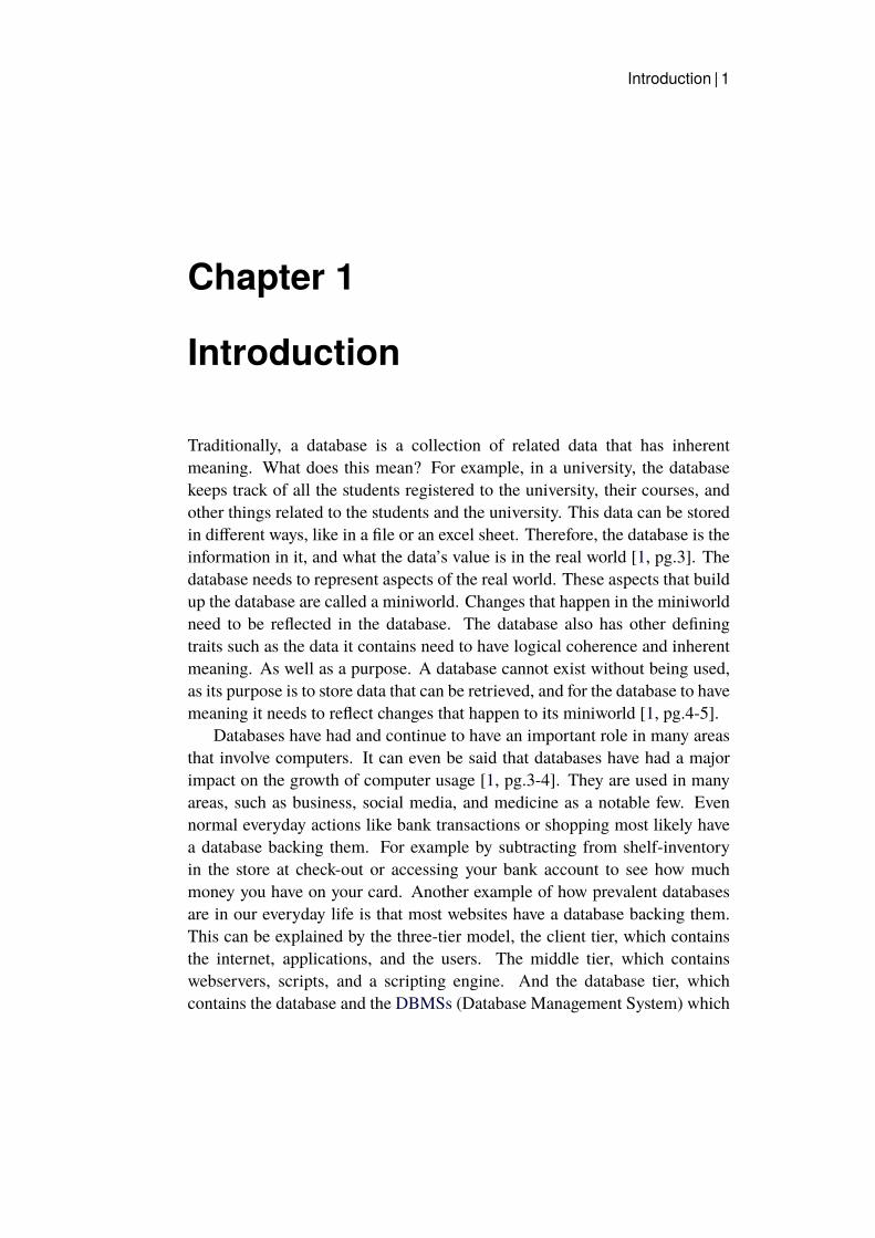
Databases have had and continue to have an important role in many areasthat involve computers. It can even be said that databases have had a majorimpact on the growth of computer usage [1, pg.3-4]. They are used in manyareas, such as business, social media, and medicine as a notable few. Evennormal everyday actions like bank transactions or shopping most likely havea database backing them. For example by subtracting from shelf-inventoryin the store at check-out or accessing your bank account to see how muchmoney you have on your card. Another example of how prevalent databasesare in our everyday life is that most websites have a database backing them.This can be explained by the three-tier model, the client tier, which containsthe internet, applications, and the users. The middle tier, which containswebservers, scripts, and a scripting engine. And the database tier, whichcontains the database and the DBMSs (Database Management System) which

Introduction | 2

Figure 1.1: The three tier database design.[3]

is used to handle the database [2]. The three-tier architecture can be seen inFigure 1.1.

What does this look like in practice? Whenever a user requests a website,the request gets sent to the webserver that requests the database to retrieveor operate on necessary data, and then finally display the results to the user[2]. Applying this logic to a social media application, logging into an accountrequires access to a database, loading the post history, or even message historyalso needs access to a database. The database is used to store the related dataand efficiently retrieve it [1, pg.4].

1.1 BackgroundNow that it has been concluded that databases are all around us and used invariety of situations, it would be very noticeable if they were slow. This isdue to how it takes just three seconds for users to drop a website if it’s stillloading, according to Sitechecker [4], which is a company that offers resourcesto analyse statistics on web pages. Their target audience is other companiesthat have some type of web traffic to monitor, and offer customer stories andratings to prove that the product they are selling is reliable.

Databases are often connected to applications - which are called databaseapplications [1, pg.9] - such as for social media. As development has broughtus faster and faster internet, internet speed can no longer be blamed for slow

Introduction | 3

access to information [5]. Therefore, it is important to maintain efficientsoftware, to have speedy responses for a good user experience. But how dowe optimise database systems for efficiency? And what is a database system?

A database system is the combination of a database and a DBMS. TheDBMS is a database software program that is often used to control the database[6]. It generally serves as an interface between the database and its usersby performing the needed operations on the database and then presenting theresult. It is in the DBMS that performance monitoring and tuning takes placeto optimise the database. The DBMS uses Structured Query Language (SQL)queries to communicate with the database from the user interface [6]. The twomain categories of database system optimisation are database tuning, whichdeals with the database hardware and design. As well as query optimisation,which mostly deals with ensuring how queries are performed in the database,which is why knowledge over SQL is important [1, pg.541, 655].

1.2 ProblemThere are several methods to optimising a database system, as stated in theintroduction, ensuring efficiency and speed is important for many differentreasons. But as there are many methods of optimisation, which ones shouldbe used? That is a question that this thesis aims to provide a starting pointfor. Having a compiled document with methods, their use cases, and howefficient they are in practice could simplify the process of choosing methods.PostgreSQL specifically is a popular open-source DBMS and providing moreinformation to the community could be valuable.

The research question is as follows:

• How do indexing and query optimisation affect response time for aPostgreSQL database?

1.3 PurposeThe purpose of this report is to describe and compare different methods foroptimising database systems. The purpose of the project is to develop anunderstanding of how database tuning and query optimisation operate. It isalso to create material that can be used for teaching purposes in databasecourses. This report should be able to lie as a starting point for furtherexperimentation and research.

Introduction | 4

1.4 Sustainability and ethicsIt can be argued that optimising a database system has an environmental effectas it reduces the resources a database uses. Shorter response time and efficientuse of hardware lead to lessening the total computing time and could reducethe wear on hardware as well as a reduction in energy usage.

An ethical problem that is related to database efficiency, is the potentialthat people more easily can manage to compile data from different data sets.This can then be presented or used to discern information that causes privacyissues.

1.5 Research MethodologyFirstly, a literature study is performed to identify methods for database tuningand query optimisation, and their different use cases. As well as to findresearch that also does these comparisons, to have as a basis for the experimentand conclusions. The study is of qualitative nature, as information that ischosen to be presented is based on what can be found, some areas might havemore information and some less. Every source was carefully examined forrelevance and trustworthiness.

After that, the experiment is planned, in part using the information foundin the literature study so that a meaningful comparison can be made. The usecases for the methods are analysed to see if there is an overlap. Lastly, data isobtained for evaluating the methods by performing an experiment. The resultis compared to the results from the literature study and is compiled in a waythat answers the research question.

1.6 DelimitationsOnly a couple of optimisation methods are chosen to study in detail, thesemethods are chosen based on the availability of information and the delimita-tions of the performed experiment. The chosen areas are database indexing -where indexes are chosen based on the available data - using the PostgreSQLoptimiser, as well as query tuning.

The delimitations of the experiment are to use PostgreSQL for the databasesystem and as a query language, the methods evaluated are limited to softwareimprovement. The database has a simple design but contains much data, andthe number of queries, indexes, and query improvements are based on the

Introduction | 5

information found, and limited to a couple of methods. The chosen methodsare based on found information and best suited for the data types used in thedatabase. These delimitations are chosen to get precise data and to ensure thatthe project will be finished in the amount of time specified for it.

1.7 Structure of the thesisChapter two presents the relevant theoretical background to understand the restof the report. As well as introduces the findings from related studies.

Chapter three describes the research methods used.

Chapter four describes the experiment parameters and how it was performed.

Chapter five compiles the results for the experiment and the literature study.

Chapter six discusses the result and the evaluation of the result and methods.

Chapter seven contains the conclusion, answers to the research question posed,and reflections about the work.

Background | 6

Chapter 2

Background

This chapter provides the basic information needed to understand the rest ofthe report, as well as some related works for the literature study. It startswith briefly going over some basics for SQL and database systems and thenmoves on to describing memory aspects of database and indexes to providea background for tuning. As well as explaining what query optimisation is,before moving on to the related works.

2.1 Database systemsThe introductory chapter briefly describes a database system as the combinationof a DBMS and the database. The more detailed description of its parts is asfollows.

2.1.1 Relational databasesA relational database stores and organises data in tables that are linked basedon related data. The purpose of this is to ensure the ability to create a newtable from data in multiple tables with a single query. It can also help withunderstanding how data is related, which could lead to improving decision-making and help identify opportunities. The tables consist of fields (columns)and the set of related data (rows) [7].

Themain benefit of using relational databases is that it reduces redundancyand through that reduces the risk for insert, update, and delete anomalies.Reduced redundancy means that, in many cases, information only appearsin one table and only once. Reducing redundancy often happens duringthe planning stages of a database, and is done by a database designer. The

Background | 7

process of doing this is called normalisation. The database designer oftenuses database schemas to start off building the database. A database schemais the structure of the database defined by formal SQL [7].

2.1.2 Database management systemsThe DBMS is a program that is used to create and maintain a database. It alsosimplifies the process of defining, manipulating, and sharing a database withmultiple users and applications. Defining the database specifies the constraintsaround it. What data types? What data structures are involved? What aresome data constraints? Are all questions that are asked during this stage ofthe process. This information is generally stored as meta-data in the DBMS’scatalogue - which is used by the DBMS software and database users to getinformation about the database’s structure. This is done because of how ageneral-purpose DBMS is not customised for a database application, so thesoftware needs to refer to the meta-data to find out what the structure is like.Constructing the database means storing data in a way that the DBMS cancontrol, and sharing the database means that multiple users and/or applicationscan access and use the database concurrently [1, pg.5-10]. Other aspects thatdefine a DBMS are insulation and the ability to have multiple views over thedata. Insulation is an aspect that ensures that the structure of data - thatis stored by the DBMS - when changed, does not affect how the programworks. This is called program-data independence. The ability to have multipleviews over data means that data from tables can be manipulated and puttogether with other tables to create other views over it. Another importantdatabase definition is the ability to reduce redundancy. Although in somecases, controlled redundancy can be used to improve query performance. Theact of reintroducing redundancy into a database is called denormalisation [1,pg.10-12, 18].

The DBMS is what is used to optimise the database. This can be donethrough the handling of effective query processing - i.e how queries areexecuted and how data is fetched etc. Tuning hardware and creating indexes isdone because of how the database often is stored on disk. This means that theDBMS needs to use special data structures, data types, and search techniquesto quickly find the data that the query is requesting. The most common wayto do this is by using indexes, as when a query is executed data needs to beretrieved from disk to main memory for processing. The entire purpose ofindexes is to improve the search process for finding and retrieving data. Thereare other ways to improve this as well, such as by tuning the hardware or

Background | 8

switching to more efficient parts. For example, the DBMS often uses cachingand buffers to improve performance. Caching means that the data retrievedfrom disk is stored for a while - there are different methods to decide for howlong - with the prediction that it might be used again. This speeds up theprocess as if the cached data gets used again the Central ProcessingUnit (CPU)does not need to wait for retrieval from disk and can just use the cache instead.The buffer helps to pipeline the process of retrieving data from disk to mainmemory, it ensures that while the CPU works on data, the next data set canget loaded into the buffer, so when the CPU is done it can immediately get thenew data. This is especially helpful if more data needs to be fetched than whatcan fit in main memory [1, pg.20, 541-558].

The DBMS consists of multiple parts. One of them is the query optimiser,which ensures that an appropriately effective execution plan is chosen for everyquery, based on some variables, such as storage system and indexes. Theexecution plan is the code that is built for the query, which decides what orderdifferent aspects of the query get executed in [1, pg.655-658]. This will bedescribed further later on in this chapter.

2.2 Structured query languageSQL is the standard language for a relational DBMSs. It is a database languagethat has statements for data definitions, queries, and updates, hence it is bothData Definition Language (DDL) and Data Management Language (DML) [1,pg.178]. DDLmeans that the query language can deal with database schemas,their descriptions, and how the data resides in the database. DML on the otherhand deals with the manipulation of data in the database, it consists of the mostcommon SQL operations [8]. The query language is used to build the databaseschemas, query the relational database, and manage the database [1, ch.6].

A database schema describes the organisation and structure of the database.It contains all the database objects, such as tables, and can be visualised asthe tables, their attributes, and how they are related to each other. In someDBMSs a database and a schema are equivalent and in others it is not [9]. Agood comparison for this can be that the database schema can be seen as a javaclass, while the database objects are the methods in the class.

2.2.1 Relational algebraRelational algebra provides a formal foundation for the relational modeloperations and is used as a basis to implement and optimise queries. It defines

Background | 9

a set of operations that can be used on a relational model. Most relationalsystems are based on relational algebra and some concepts are defined inSQL. Therefore, a query can be translated into a sequence of relational algebraoperations, also called a relational algebra expression [1, ch.8].

It is assumed that the readers are familiar with relational algebra, whichmeans the report will not go into detail about it.

2.2.2 PostgreSQLPostgreSQL is an open-source object-relational database system that usesSQL, and offers features such as foreign keys - reference keys that link tablestogether - updatable views and more [10]. Views will be described in the nextsubsection.

PostgreSQL can also be extended by its users by adding new data types,functions, index methods, and more [10]. Its architecture is a client/servermodel, and a session consists of a server process - that manage databasefiles, accepts connections to the database from the client-side, and performsdatabase operations requested by the clients. And the client application thatrequests database actions for the server to perform. Like a typical client/serverapplication, the server and client do not need to be connected to the samenetwork and can communicate through normal internet procedures. This isimportant to keep in mind as files on the client-side might not be accessibleon the server-side. PostgreSQL can handle multiple client connections to itsservers [11] as most servers can.

Earlier it was mentioned that PostgreSQL is a relational database manage-ment system. This means that it is a system for managing data stored inrelations - the mathematical term for a table. There are multiple ways oforganising databases [12], but relational databases are what is the focus ofthis report. Each table in a relational database system contains a collectionof named rows, and each row has a collection of named columns that containa specified data type. These tables are then grouped into database schemas.There can be multiple databases in one server, just like there can be multipleschemas in a database. A collection of databases managed by one PostgreSQLserver is called a database cluster [12]. Another aspect of PostgreSQL is that itsupports automatic handling of foreign keys, through accepting or rejecting thevalue depending on its uniqueness. This means that PostgreSQL will warn ifthe value in the foreign key column is not unique, which is done to maintain thereferential integrity of the data. The behaviour of the foreign key can be tunedto the application by the developer [13], this can be done through specifying

Background | 10

deletion of referenced objects, the order of deletion, and other things [14].

2.2.3 QueriesHere some query concepts used in the experiment will be explained.

Query operations

Two of the query operations that are used in the experiment need some closerexamination. The LIKE and IN operations. To do this, the PostgreSQLtutorial’s website is used. PostgreSQL tutorial is a website dedicated toteaching PostgreSQL concepts. They show examples and explanations of howto use operations and build a database [15].

The LIKE operation is used to pattern match strings to each other. Thiscan be done using wildcards, which in PostgreSQL is ’%’ for any sequenceof characters and ’_’ for any single character. A wildcard is used for patternmatching, as stated before. For example, matching the string ’Jen%’ couldgive any string that starts with ’Jen’. While using ’Jen_’ could match anystring starting with ’Jen’ and then a single character after [16].

The IN operator is used to match any string within a list of values. It doesthis by returning true if the comparing string matches one of the stated valuesin the IN operation. It is the equivalence of using equals and OR operations,although PostgreSQL executes the IN queries faster than the OR queries [17].

Nested queries

A query that executes multiple queries in one contains an inner query - alsocalled a subquery - and an outer query [18]. Often these types of queries canbe split into multiple separate queries. PostgreSQL executes these queries byfirst, executing the inner query, then getting the result and passing it to theouter query. Lastly, it executes the outer query [18].

A correlated inner query is evaluated for each row that is processed by theouter query, which differs from how a normal nested query executes accordingto Geeks for Geeks, a website dedicated to learning programming languagesthrough examples [19]. As mentioned in the paragraph earlier, in a normalnested query the inner query gets executed first and then the outer query. Itcan also be said that the correlated query is driven by the outer query as theresult of the inner query is dependent on the outer query [19]. This workssimilarly to how nested loops work in any other programming language.

Background | 11

2.2.4 Views and materialised viewsA view is a named query that is often useful to have for queries that are runoften. It is a key aspect of a good SQL database design. Views can be usedin almost any place a real table can, and it is possible to build multiple viewson each other [20]. Although, it is important to note that views are not storedas tables, and are instead stored as references to the queries. This means thatevery time a view is called on, the query that it is based on is executed [21].

The materialised view uses the same system as a view does but stores theresult like a table. Themain difference between amaterialised view and a tableis that the materialised view cannot be updated. Instead, the query that createsthe materialised view is stored, so that it can be refreshed when the data needsto be updated. The data is often faster to access through a materialised viewthan a table, which can be useful in many cases even if the data is not entirelyup to date [22].

2.3 Database tuningThe goal of database tuning is to dynamically evaluate the requirements -sometimes periodically - and to reorganise indexes and the file order to gain thebest over-all performance. This makes changes to the database and its structurethrough normalisation or denormalisation, indexes, and the hardware aspectof the database - such as how files are physically ordered on disk, optimisingInput/Output (I/O) operations, hardware upgrades et cetera [1, pg.459-461,640].

Normalisation, denormalisation, and some aspects of hardware are outsideof the scope of this report and will not be discussed further but some memoryaspects are important to be aware of, this is discussed in the next subsection.

2.3.1 Database memoryA database is often too large to store in main memory, thus to manageperformance a basic understanding of how database hardware works arenecess-ary. The memory structure of a database is usually separated intothree parts [1, pg.542]. The primary storage, which is what the CPU useswhen executing operations. The secondary storage most usually consistsof Hard Disk Drives (HDDs) or Solid State Drives (SSDs), and lastly thetertiary storage, which is offline storage such as Compact Disks (CDs) andmagnetic tapes. The most important aspect for optimisation of memory access

Background | 12

is bringing data to the primary storage from the secondary storage, for theexecution of operations on the database. In some cases, a database can bestored in the primary memory - a so-called main memory database - thisis often done for real-time applications. But because databases often storepersistent data, some of which needs to be read or handled multiple timeswhile it is stored, it needs to use secondary storage. The databases are alsogenerally too big to store on a single disk which means that multiple disks needto be used, and the benefits of secondary storage hardware often outweigh thebenefits of the primary storage ones [1, pg.542-544].

Typically, the database application only needs small amounts of data toprocess from the database, hence, the data needs to be accessed on disk andeffectively moved to main memory to increase the speed of execution. Asmentioned earlier this is partly done through hardware by the use of buffers,as there is a noticeable difference between how quickly the CPU can processdata and the moving of data from disk to main memory. Other ways to do thisrequire a basic understanding of how the data is stored in the database and thehardware.

The data on disks are stored as something called files of records, in which arecord is a set of data values that describe entities, their attributes, and relations- i.e a table [1, pg.560]. Files of records are often stored in data blocks - alsocalled a page - which are fixed sizes of storage on a disk. This is importantto note as the transmission of data from disk to main memory usually is doneon a per-block basis. By physically storing data in contiguous blocks on diskperformance can be improved as it puts related data near each other, which canprevent the arm on the disk (HDD) from having to move longer distances. Thiscan be further improved by prediction, which is done through reading multipleblocks of data at once and putting it in main memory. This can reduce thesearch time on disk access. It only works if the application is likely to needconsecutive blocks and the ordering of the file organisation allows it, though[1, pg.561-563].

How files are ordered in memory can be done in different ways. Storingthe files in a specific order is called the file organisation [23], and it can bedescribed as the auxiliary relationship between the records that build up thefile. It is used to identify and access any given record [1, pg.545-546]. In thedatabase, there are two ways to store files, the primary file organisation andthe secondary file organisation. The primary file organisation decides howfile records are physically placed on disk. This is done by using different datastructures such as heaps, hash structures, and B-trees. For example, a heap filewould not store the records in any particular order and instead place them as a

Background | 13

heapwould order them. Unlike the primary file organisation, the secondary fileorganisation is a logical access structure that improves the access to file recordsbased on other fields than what is used for the primary file organisation. Thisis often done through indexing [1, pg.545-546, 604-611].

There can be different types of records in a file, the type is decided bythe collection of field names and their corresponding data types contained inthe record. This means that records in files can be constant or of variablelength. If a file has variable length records it can affect indexing and searchalgorithms efficiency. This is due to the way files consist of sequences ofrecords. By having a constant length on records it is simpler to calculate thestart of each field in a record based on the relative starting point of the recordin the file. Therefore, algorithms handling variable-length records often needto be more complex, which can affect the speed of execution [1, pg.560-561].The different ways of how variable-length files can look are as follows:

• The file record is of the same type but one or more of the fields havedifferent sizes.

• The file record is of the same type but one or more of the fields havemultiple values for each record, this is called a repeating field.

• The file record is of the same type but one or more of the fields are notmandatory.

• The file contains one or more records of different record types, this leadsto the records being of different sizes. This often happens in clusters ofrelated records.

[6, pg.]60-5611

As mentioned earlier, there are heap files and ordered files, which are themain ways of storing records on a file. The heap files store records in a heapstructure, while the ordered files can use many different data structures forstorage. The main benefit of using ordered files is that other search algorithmsthan linear search can be used when searching for a record. Although, orderedfiles are rarely used unless a primary index is implemented [1, pg.567-572].The main data structures implemented for ordered files are hash tables, hashmaps, and B-trees, which each have their pros and cons and are chosendepending on what the file is used for [1, pg.583]. These data structures aredescribed in more detail later on in this chapter.

Background | 14

2.3.2 IndexingAn index is a supplementary access structure. It is used to quickly find andretrieve a record based on specified requirements. They are stored as files ondisk and contain a secondary access path to reach records without having tophysically order the files [1, pg.601-602]. Without an index, a query wouldhave to scan an entire table to find the entries it is searching for. In a big table,having to go through every element sequentially would be very inefficient,especially in comparison to using an index. For example in a b-tree index, thesearch would only need to go a couple of levels deep in the tree [1, pg.601-602]. The index is handled by the DBMS in PostgreSQL. Which in parthandles the updates for the index when a table changes. The downside tousing indexes is that updating them as the tables change adds an overhead tothe data manipulation operations. This means that updating a table indirectlyadds to the execution time of the data manipulation operations [24], which isan important aspect to keep in mind when deciding if an index should be builton a table or not [1, pg.601].

The indexes are based on an index field, which can be any field in a file ormultiple fields in the file. Multiple indexes can also be created on the samefile. As mentioned earlier, indexes are data structures used to improve searchperformance. Therefore, many data structures can be used to construct them.The data structure is chosen depending on many different factors. One suchfactor is what queries are predicted to be used on the index. Indexes can beseparated into two main areas, single-level indexing and multilevel indexing[1, pg.601], which will be described below.

Single-level indexes

Single-level indexing using ordered elements has the same idea as a bookindex, which has a text title and the page it can be found on. This can becompared to how the index has the index field and the field containing thepointers to where the data can be found on disk. The index field used forbuilding the index on a file - with multiple fields - with a specified recordstructure, is usually only based on one field. Like earlier mentioned, the indexstores the index field and a list of pointers to each disk block that contains arecord with the same index field. The values - index fields - in an orderedindex are also sorted so that a binary search can be performed to quickly findthe desired data. How efficient is this? Well, if a comparison is made in thecase of having both the data file and the index file sorted, the index file is oftensmaller than the data file. This means that searching through the index is still

Background | 15

faster than through the data file [1, pg.602].As stated in the background, the index types are often separated into

primary and secondary indexes. The single-level index can be either of thesetypes [1, pg.602].

A primary index is a file containing ordered keys for a sorted file record.The primary index is used to physically order data on disk, which means thata primary index can only be a single-level index and that there can only be oneprimary index on a table. The field for the key is used to physically order thefiles, each record must have a unique value for that to be possible. The primaryindex only contains two fields, as stated earlier, which makes it effective forsearching for data records in a file. The first field is a primary key and thesecond field is a pointer to a block address on disk. There is one index entryfor each block in the data file. Although, a primary index does not have to usea key for the ordering field, and if it does not use a key it is called a clusteredindex instead [1, pg.602.605].

Indexes can also be defined as compact or sparse indexes. A sparse indexhas fewer entries than there are records on a file, which by definition makes aprimary index a sparse index. The main issue with a primary index - as is theissue for most sorted data structures - is the insertion and deletion of elements.For example, inserting a new element in a filled array requires expansion of thearray, and in a linked list, searching for where to insert the element takes time.Cluster indexes are used to quickly find groups of data. It is also an orderedindex that has to deal with the issues of insertion and deletion of records.To solve this, clustered indexes often reserve space in blocks for insertion.Both cluster and primary indexes assume that the field for physical orderingof records on disk is the same as the index field [1, pg.602-605].

A secondary index offers a second logical ordering alternative for accessinga file when a primary option already exists. The records on the data file can beordered, unordered, or hashed, as it does not deal with the physical orderingof records. The secondary index is also an ordered file with two fields, like aprimary index. But it is created on a field with a candidate key or that has aunique value in each record. A candidate key is a field that could be a primarykey, and a primary key is a field - or fields - that can be used to uniquely identifya row. This can be done by using counters, but also through othermeans. Therecan be multiple candidate keys, but only one primary key, which means thatmultiple secondary indexes can be created for the same file. In practice, itjust adds access paths to the file based on different fields. Secondary indexesoften take more memory space than primary indexes, although searching forarbitrary records is noticeably quicker [1, pg.609-611].

Background | 16

Multi-level indexes

The idea behind a multilevel index is to reduce the part of the index that issearched with the block factor (bfri) - also called the fan-out (fo) - for theindex. During a multilevel index search, the area that is searched is reducedby fo, which if larger than two makes it more efficient than binary search. Theway the multi-level index works is by viewing the index file as an ordered filewith a distinct value for each entry. The index file counts as the first levelof the multi-level index and the second level is defined as the primary indexthat is created on the first level. A block anchor is created for the secondlevel so that it has an entry for each block of the first level. The block factorremains the same for every level of the multi-level index as the size for entriesremains the same - a field value and a block address. This process is then berepeated, level three is another primary index created on the second level, etcetera. More levels are only needed if a level needs more than one block forstorage as each level reduces the number of entries by a factor of fo, this meanseach level requires less storage. This also means that only one disk block isaccessed per level, thus, for a multi-level index with t levels only t disk blocksare accessed during a search. Which increases the speed of searches. Lastly,the last level of the index is called the top index level, and the multi-levelindex can use primary, secondary and cluster indexes [1, pg.613-614]. Multi-level indexes still suffer from the issues of insertion and deletion of records.Dynamic multi-level indexes aim to solve this by leaving space in blocks forinsertion of new entries and using appropriate insertion/deletion algorithmsfor creating/deleting index blocks when the data file grows/shrinks. This isoften done by using B+-trees - which functions like a B-tree but has its leafnodes connected as well - as a data structure [1, pg.613-614].

2.3.3 Index typesPostgreSQL provides multiple index types, among them are B-trees, Hashstructures, Generalised Search Tree (GiST), Space Partitioned GeneralisedSearch Tree (SP-GiST), Generalised Inverted Index (GIN) and Block RangeIndex (BRIN). The index types use different algorithms that are better suitedfor different types of queries. The B-tree usually suits the broadest range ofqueries which is why the default index type used for PostgreSQL is the B-tree[25].

Background | 17

B-trees

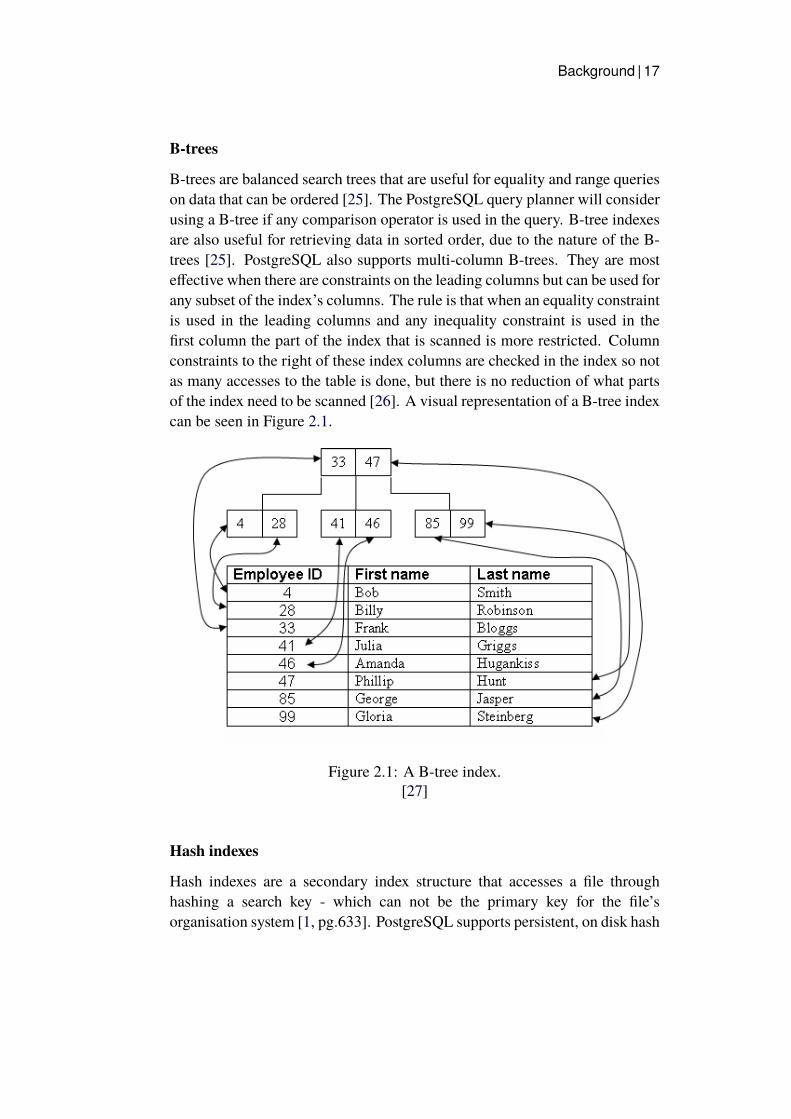
B-trees are balanced search trees that are useful for equality and range querieson data that can be ordered [25]. The PostgreSQL query planner will considerusing a B-tree if any comparison operator is used in the query. B-tree indexesare also useful for retrieving data in sorted order, due to the nature of the B-trees [25]. PostgreSQL also supports multi-column B-trees. They are mosteffective when there are constraints on the leading columns but can be used forany subset of the index’s columns. The rule is that when an equality constraintis used in the leading columns and any inequality constraint is used in thefirst column the part of the index that is scanned is more restricted. Columnconstraints to the right of these index columns are checked in the index so notas many accesses to the table is done, but there is no reduction of what partsof the index need to be scanned [26]. A visual representation of a B-tree indexcan be seen in Figure 2.1.

Figure 2.1: A B-tree index.[27]

Hash indexes

Hash indexes are a secondary index structure that accesses a file throughhashing a search key - which can not be the primary key for the file’sorganisation system [1, pg.633]. PostgreSQL supports persistent, on disk hash

Background | 18

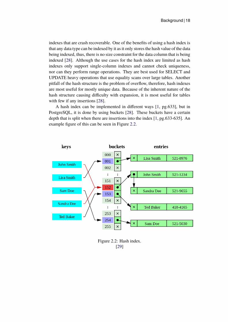
indexes that are crash recoverable. One of the benefits of using a hash index isthat any data type can be indexed by it as it only stores the hash value of the databeing indexed, thus, there is no size constraint for the data column that is beingindexed [28]. Although the use cases for the hash index are limited as hashindexes only support single-column indexes and cannot check uniqueness,nor can they perform range operations. They are best used for SELECT andUPDATE heavy operations that use equality scans over large tables. Anotherpitfall of the hash structure is the problem of overflow, therefore, hash indexesare most useful for mostly unique data. Because of the inherent nature of thehash structure causing difficulty with expansion, it is most useful for tableswith few if any insertions [28].

A hash index can be implemented in different ways [1, pg.633], but inPostgreSQL, it is done by using buckets [28]. These buckets have a certaindepth that is split when there are insertions into the index [1, pg.633-635]. Anexample figure of this can be seen in Figure 2.2.

Figure 2.2: Hash index.[29]

Background | 19

GiST indexes

A GiST index is a type of index that can be tweaked by the developer asthere are many different kinds of index strategies that can be implemented[25]. It is based on the balanced tree access method to use for arbitraryindexing schemes. The main advantage to using GiST is that it allows forthe development of a custom data type with an appropriate access structureby a data type expert - a programmer that does not have to be a databaseadministrator [30]. How the GiST index is used depends on what operatorclass is implemented, but the standard for PostgreSQL is to include severaltwo-dimensional geometric data types [25]. The operator class defines whatoperators can be used on the columns in the index, for example, comparisonoperations between different data types [31]. GiST indexes can optimisenearest-neighbour searches, but this is dependent on the operator classesdefined [25]. A multi-column GiST can be used with query conditions thatuse any subset of the index’s columns. Adding additional columns restrictsthe entries returned by the index. The way this works is that the first columnis used to determine how much of the index need to be scanned. This index isnot very effective if the first column only has a few distinct values [26].

SP-GiST indexes

SP-GiST indexes expand onGiST indexes by permitting the implementation ofdifferent non-balanced disk-based data structures, such as radix trees, tries etcetera [25]. It supports partitioned trees which allow developing non-balancedtree structures. The generally desired feature for the structures is to use it todivide the search into pieces of equal size [32]. The standard operators for anSP-GiST index in PostgreSQL is to use an operator class for two-dimensionalpoints [25].

GIN indexes

GIN indexes are similar to the previous two ones, although it differs by usingthe standard operator class for standard array operators [25]. GIN is speciallydesigned to handle when the items to be indexed are composite values, andthe queries performed need to search for the element values in the compositeitems. The word item refers to the composite values to be indexed and thekey is the element value. The way the GIN works is that it stores sets ofpairs - with the key and the posting list. The posting list is a set of rowsIdentity Documents (IDs) where the keys occur. Each key-value is only stored

Background | 20

once even though the same ID can occur multiple times [33]. Multi-columnGIN indexes work similar to multi-column GiSTs, the main difference is thatthe search effectiveness is not dependent on what index column the queryconditions use [26].

BRIN indexes

BRIN indexes store summaries of the values in a table in consecutive physicalblock ranges [25]. It is designed to handle very large tables that have columnswith some natural correlation to where the columns are physically storedwithin the table. BRIN indexes can perform queries with regular bitmap indexscans which returns all tuples in all pages - within a specified range - if thesummary information stored by the index is part of the query conditions. Thissummary information needs to be updated when new pages of data are filled.This is not done when a new page is created, it is instead created when asummarisation run is invoked. On the other hand, values in a table changingcan also cause the index tuple in the summary to be inaccurate. TO solve this,de-summarisation can be run [34]. The operator class that BRIN uses dependson the implemented strategies. For data with linear store order, the data in theindex usually correspond to theminimum andmaximum values of the columnsfor each block range, which makes some operations more suitable than others.But as different types of data can be stored in this type of index, the operationsneed to be chosen based on the type of data [25]. Multi-column BRIN indexes,like GIN has no dependence on what column is used in the query condition.Although there are few reasons as to why a multi-column BRINwould be used[26].

More about PostgreSQL indexes

PostgreSQL can combine multiple indexes, including multiple uses of thesame type of index. This is useful when there are cases where a single indexscan done by a query cannot directly use the index, which can happen if valuesare missing in the index that the query needs. To combine multiple indexes,the system creates a bitmap over each needed index. It maps the location oftable rows that matches the index conditions, and the table rows are visited inphysical order as that is how a bitmap works. This means that the ordering inthe indexes is lost, and a separate sort needs to be applied if the query requestsordering of elements [35]. Another index that is supported by PostgreSQL isthe partial indexes that are built over a subset of a table, which PostgreSQLalso supports. Another reason to use partial indexes is that it can help avoid

Background | 21

indexing common values, since querying common values most often do notuse indexes anyways. This reduces the size of the index so that many tableoperations are sped up when performed on the index [36].

All indexes are secondary indexes in PostgreSQL. This means that thetable rows that are referenced can be anywhere on the PostgreSQL data heap.To access the data from an index scan, therefore, involves random access.Which depending on the disk drive can be slow. To make this more efficient,something called an index-only scan is supported. What this means is thata query can be answered without accessing the heap. The idea behind itis to return index entries instead of consulting with the heap entries. InPostgreSQL, only B-trees, GiSTs and SP-GiSTs can support index-only scans,and only B-trees always has built-in support for it [37]. One requirement todecide if an index-only scan is possible to form is that the query that wantsto use the index-only scan must only reference columns that are stored inthe index, otherwise, heap access is needed. Another requirement for index-only scans is that each row retrieved is visible to the query’s Multi-VersionConcurrency Control (MVCC) snapshot [37]. The MVCC is something thatPostgreSQL uses for concurrency control. It works by showing each queryand transaction a snapshot of how the database was some time ago, nomatter how the data looks at the exact moment of querying. This protectsthe transaction from seeing inconsistent data that could be caused by otherconcurrent transactions [38]. The visibility information is not stored in theindex, but PostgreSQL keeps track of the data that is old enough that it shouldbe visible for all future transactions. This means that there is a loophole fordata that does not change often to use index-only scans [37]. To effectivelyuse this feature, a covering index can be used. This type of index is designedto include columns needed by a specified query. Sometimes some columnsthat are not part of the result is needed for a query, PostgreSQL supportsthis by adding a payload that is not part of the search key with the commandINCLUDE [37], this can also be used to solve the problem of missing valuesin indexes like discussed for combining indexes.

2.3.4 Tuning variablesThere are many factors to consider when building the physical database designto ensure efficiency. Among them are analysing queries to optimise thestructure of tables and indexes. This is done to ensure that indexes are usedand as efficient as predicted. the variables that each retrieval query looksat to map efficiency are: the relations accessed by the query, the attributes

Background | 22

on which a selection condition is specified, what type of condition it is, theattributes of any join or multiple tables, or objects that are linked and theattributes whose values will be retrieved by the query [1, pg.643-646]. Aswell as for each update operation or transaction: the updated files, the type ofoperations on each file, the attributes that the selection condition specifies, andthe attributes whose values will be changed by the updates need to be assessed.The expected frequency of invocation of queries and transactions, as well asthe time constraints of them also needs to be analysed. These aspects also needto be considered for update operations and uniqueness constraints on attributes[1, pg.643-646].

The initial choice of indexes might need to change for many differentreasons, some of them might be due to the reasons listed in the previousparagraph. Other reasons are listed below:

• Queries might take too long to run due to lack of indexing.

• Some indexes might not be used by the queries.

• Some indexes are updated too frequently because the index attributechanges too often.

[1, pg.640]

To figure out if any of these issues apply to the database, many DBMSs havecommands for tracing how a query is executed. After doing that the issuescan be solved by either dropping, creating, or changing indexes (to or fromcluster indexes), and rebuilding the indexes. All of these options can improveperformance if the tracing is read correctly. The reasonwhy rebuilding indexescan improve performance is because of how in the case of there being manydeletions on the index key the index pages may contain space that is not used.This space can then be reclaimed during a rebuild. Rebuilding can also solveoverflow issues caused by insertions [1, pg.640].

2.4 Query optimisationQuery optimisation is the action of finding the best possible way for a queryto be executed, based on the physical database structure and indexes available.Although optimisation is not the best word for it, as there needs to be a limitfor how long it can take before a query needs to be executed, which means thatthe optimal execution path might not be found. All of this is done by the queryoptimiser in the DBMS and can be implemented in different ways [1, pg.655].

Background | 23

2.4.1 The query optimiserThe purpose of the optimiser is to create a good query plan, as stated earlier.This is done by the DBMS to retrieve results from the database file. This planis then translated to code by the code generator, which is done in three steps:the first step is to scan a query to identify all the query tokens. In the secondstep, the parser checks the syntax, and the validator checks all the attributesand relation names. Thirdly, a query tree structure or a Directed A-cyclicalGraph (DAG) is created as an internal representation of the query. There aremany different execution strategies for a query and the process of choosingone of them is what query optimisation is all about [1, pg.655-658].

As earlier mentioned, optimisation is not the best term for this process,as most of the time, the optimal plan is not chosen. Rather a reasonablyefficient plan is. Finding the optimal strategy is too time-consuming - thereis an exception for simple queries - as there are many variables involved whentrying to find an optimal strategy. Such as detailed information about the sizesof the table, the distributions of column values, and the expected size of theresult. Some of this information is not available for the DBMS. Despite this,optimisation is still needed in relational databases since SQL is a high-levelquery language. This means that there is only a specification of the intendedresult, not how to get there [1, pg.655-658].

To do all this the query optimiser first translates the query into an equivalentextended relational algebra expression. This is the tree mentioned for thequery plan. It is used to transform the query into an optimised one. The waythis is done is most often by deconstructing the query into query blocks, thatthen are translated into algebraic expressions [1]. After that, the optimisercan choose the best query plan for each block. This is done by improving onthe algebraic expressions, and by following a set of heuristic rules. In whichone of the most important rules is to preserve equivalence. This is due tothere being many algebraic expressions to represent the same query. Whilethe query is optimised it is not allowed to get switched into something else.The equivalence preservation rules ensure that the algebraic expressions forqueries remain equivalent [1, ch.18].

2.4.2 The PostgreSQL optimiserThe PostgreSQL optimiser creates a query plan for every query it receives.With the EXPLAIN command, it is possible to access what plans the plannermakes for any query. The structure of the planner is a plan tree with plan nodes,in which the leaf nodes of the tree are scan nodes that return rows from a table.

Background | 24

There are different types of scan nodes depending on the type of scan that isperformed. If the query has other operations such as join, sorting, et ceterathere will be nodes above the scan nodes - which means that the tree growsupwards [39]. As there are different ways to perform these operations, othernodes can also appear. The output of EXPLAIN shows a line for each nodein the plan tree, its type, and the estimated cost of the execution of that node.The costs are estimated in arbitrary units that are dependent on the planner’scost parameters. The cost of an upper level-node includes the cost of all itschildren nodes.

An important thing to keep in mind is that the planner only will considerthings it cares about in the cost, transmitting the result is not one of them. Thisis important to note as there can be other things that affect efficiency that theplanner does not count on [39], which could mean that optimising a query isnot the best solution to all efficiency problems.

To check the accuracy of the planners estimate the command EXPLAINANALYZE can be used. This causes the EXPLAIN command to execute thequery and then display the row count and the run time for each plan nodeas well as their estimates. For the executed plans the unit is in millisecondsinstead of an arbitrary unit, which is used by the statistics that EXPLAINshows. EXPLAIN also has other options, among them is a BUFFER optionthat further can help with analysing run time statistics. This is done throughhelping with analysing what I/O operations are the most sensitive [39].

It is also important to note that with EXPLAINANALYZE the transactionsneed to be rolled back as the query is executed [39]. There are also otherpitfalls to using EXPLAIN ANALYZE, such as the statistics deviating fromnormal run-time execution time. One reason as to why this happens is dueto no output rows being delivered to a client. This means that there isno consideration to transmission time and I/O conversion costs. Anotherissue is that the overhead to EXPLAIN ANALYZE can be significant, thisis because of how different operating systems can have different speeds fortheir gettimeofday() operations, so the operation can take longer than actualexecution time due to this. The last pitfall to keep in mind is that EXPLAINresults cannot be generalised among different tables. This means that the sameresult cannot be expected to apply on a large table when tested on a small table[39].

The query planner looks at statistics to make good estimates, it does thisfor specific variables. For single-column statistics, important factors are thetotal number of entries in each table, and index, as well as the disk blocks theyoccupy. This information is kept as part of the table in the pg_class, under

Background | 25

the names reltuples and relpages. These two columns are not updated veryoften, so they often contain old values. VACUUM or ANALYZE can be usedto update them on a per-use basis, which means that they are incrementallyupdated as they are used [40].

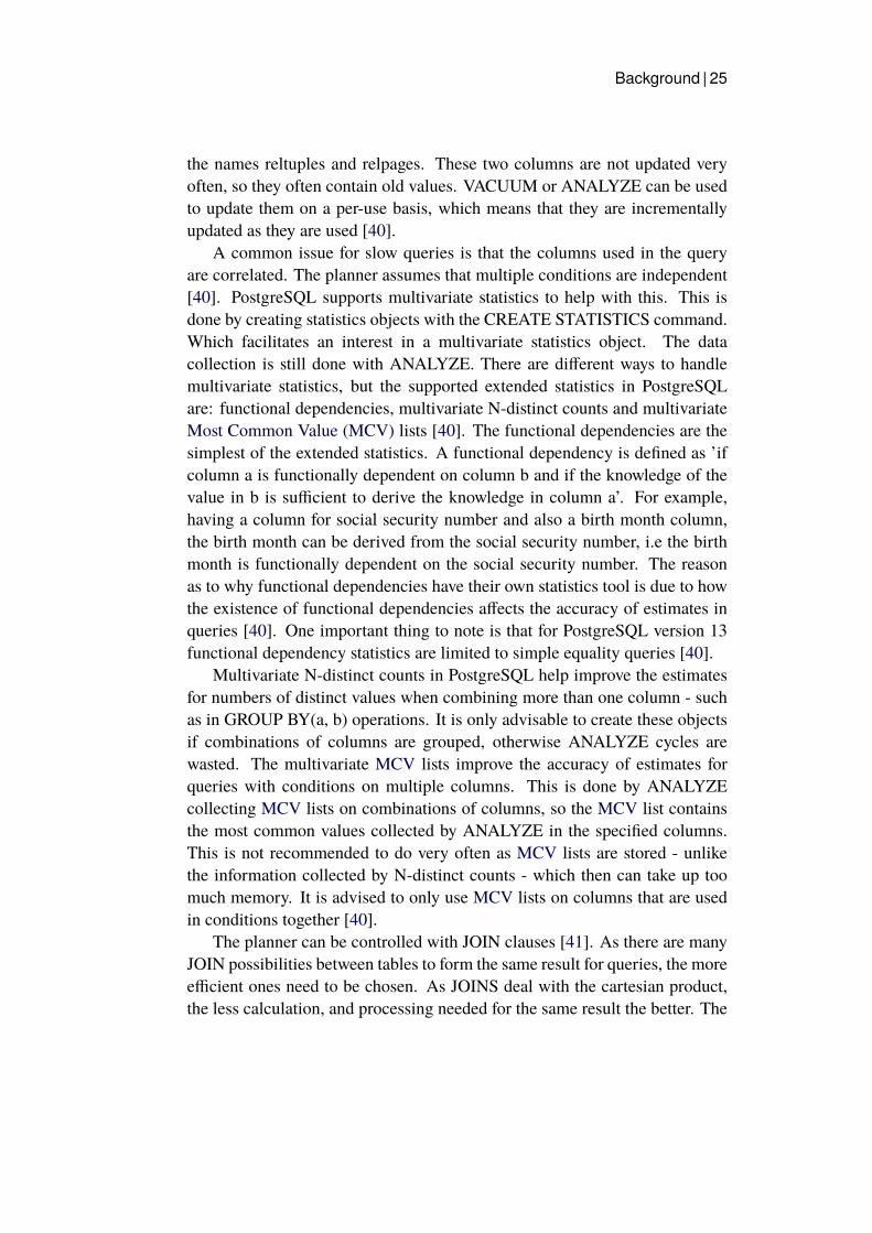
A common issue for slow queries is that the columns used in the queryare correlated. The planner assumes that multiple conditions are independent[40]. PostgreSQL supports multivariate statistics to help with this. This isdone by creating statistics objects with the CREATE STATISTICS command.Which facilitates an interest in a multivariate statistics object. The datacollection is still done with ANALYZE. There are different ways to handlemultivariate statistics, but the supported extended statistics in PostgreSQLare: functional dependencies, multivariate N-distinct counts and multivariateMost Common Value (MCV) lists [40]. The functional dependencies are thesimplest of the extended statistics. A functional dependency is defined as ’ifcolumn a is functionally dependent on column b and if the knowledge of thevalue in b is sufficient to derive the knowledge in column a’. For example,having a column for social security number and also a birth month column,the birth month can be derived from the social security number, i.e the birthmonth is functionally dependent on the social security number. The reasonas to why functional dependencies have their own statistics tool is due to howthe existence of functional dependencies affects the accuracy of estimates inqueries [40]. One important thing to note is that for PostgreSQL version 13functional dependency statistics are limited to simple equality queries [40].

Multivariate N-distinct counts in PostgreSQL help improve the estimatesfor numbers of distinct values when combining more than one column - suchas in GROUP BY(a, b) operations. It is only advisable to create these objectsif combinations of columns are grouped, otherwise ANALYZE cycles arewasted. The multivariate MCV lists improve the accuracy of estimates forqueries with conditions on multiple columns. This is done by ANALYZEcollecting MCV lists on combinations of columns, so the MCV list containsthe most common values collected by ANALYZE in the specified columns.This is not recommended to do very often as MCV lists are stored - unlikethe information collected by N-distinct counts - which then can take up toomuch memory. It is advised to only use MCV lists on columns that are usedin conditions together [40].

The planner can be controlled with JOIN clauses [41]. As there are manyJOIN possibilities between tables to form the same result for queries, the moreefficient ones need to be chosen. As JOINS deal with the cartesian product,the less calculation, and processing needed for the same result the better. The

Background | 26

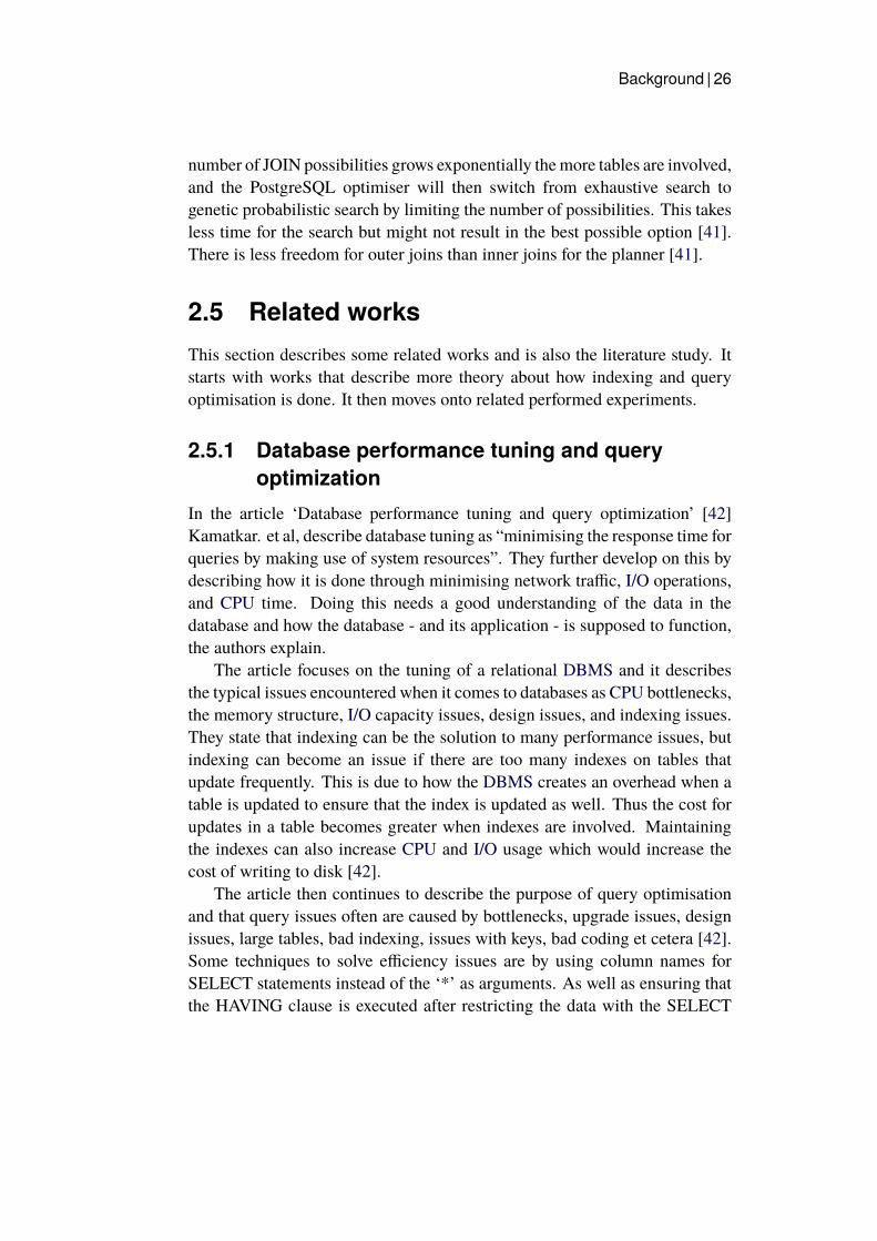
number of JOIN possibilities grows exponentially themore tables are involved,and the PostgreSQL optimiser will then switch from exhaustive search togenetic probabilistic search by limiting the number of possibilities. This takesless time for the search but might not result in the best possible option [41].There is less freedom for outer joins than inner joins for the planner [41].

2.5 Related worksThis section describes some related works and is also the literature study. Itstarts with works that describe more theory about how indexing and queryoptimisation is done. It then moves onto related performed experiments.

2.5.1 Database performance tuning and queryoptimization

In the article ‘Database performance tuning and query optimization’ [42]Kamatkar. et al, describe database tuning as “minimising the response time forqueries by making use of system resources”. They further develop on this bydescribing how it is done through minimising network traffic, I/O operations,and CPU time. Doing this needs a good understanding of the data in thedatabase and how the database - and its application - is supposed to function,the authors explain.

The article focuses on the tuning of a relational DBMS and it describesthe typical issues encountered when it comes to databases as CPU bottlenecks,the memory structure, I/O capacity issues, design issues, and indexing issues.They state that indexing can be the solution to many performance issues, butindexing can become an issue if there are too many indexes on tables thatupdate frequently. This is due to how the DBMS creates an overhead when atable is updated to ensure that the index is updated as well. Thus the cost forupdates in a table becomes greater when indexes are involved. Maintainingthe indexes can also increase CPU and I/O usage which would increase thecost of writing to disk [42].

The article then continues to describe the purpose of query optimisationand that query issues often are caused by bottlenecks, upgrade issues, designissues, large tables, bad indexing, issues with keys, bad coding et cetera [42].Some techniques to solve efficiency issues are by using column names forSELECT statements instead of the ‘*’ as arguments. As well as ensuring thatthe HAVING clause is executed after restricting the data with the SELECT

Background | 27

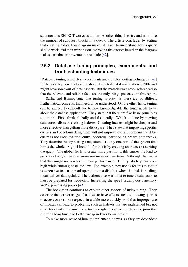
statement, as SELECT works as a filter. Another thing is to try and minimisethe number of subquery blocks in a query. The article concludes by statingthat creating a data flow diagram makes it easier to understand how a queryshould work, and then working on improving the queries based on the diagrammakes sure that improvements are made [42].

2.5.2 Database tuning principles, experiments, andtroubleshooting techniques

‘Database tuning principles, experiments and troubleshooting techniques’ [43]further develops on this topic. It should be noted that it was written in 2002 andmight have some out-of-date aspects. But the material was cross-referenced sothat the relevant and reliable facts are the only things presented in this report.

Sasha and Bonnet state that tuning is easy, as there are no difficultmathematical concepts that need to be understood. On the other hand, tuningcan be incredibly difficult due to how knowledgeable the tuner needs to beabout the database application. They state that there are five basic principlesto tuning. First, think globally and fix locally. Which is done by movingdata across disks or creating indexes. Creating indexes might be cheaper andmore effective than getting more disk space. They state that improving specificqueries and bench-marking them will not improve overall performance if thequery is not executed frequently. Secondly, partitioning breaks bottlenecks.They describe this by stating that, often it is only one part of the system thatlimits the whole. A good local fix for this is by creating an index or rewritingthe query. The global fix is to create more partitions, this causes the load toget spread out, either over more resources or over time. Although they warnthat this might not always improve performance. Thirdly, start-up costs arehigh while running costs are low. The example they use is for this is that itis expensive to start a read operation on a disk but when the disk is reading,it can deliver data quickly. The authors also warn that to tune a database onemust be prepared for trade-offs. Increasing the speed usually costs memoryand/or processing power [43].

The book then continues to explain other aspects of index tuning. Theydescribe the correct usage of indexes to have effects such as allowing queriesto access one or more aspects in a table more quickly. And that improper useof indexes can lead to problems, such as indexes that are maintained but notused, files that are scanned to return a single record, and multi-table joins thatrun for a long time due to the wrong indexes being present.

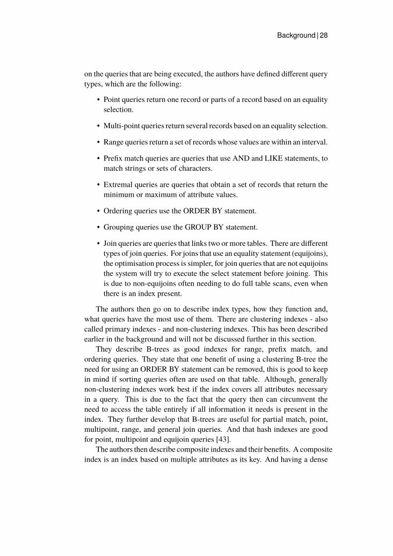
To make more sense of how to implement indexes, as they are dependent

Background | 28

on the queries that are being executed, the authors have defined different querytypes, which are the following:

• Point queries return one record or parts of a record based on an equalityselection.

• Multi-point queries return several records based on an equality selection.

• Range queries return a set of records whose values are within an interval.

• Prefix match queries are queries that use AND and LIKE statements, tomatch strings or sets of characters.

• Extremal queries are queries that obtain a set of records that return theminimum or maximum of attribute values.

• Ordering queries use the ORDER BY statement.

• Grouping queries use the GROUP BY statement.

• Join queries are queries that links two or more tables. There are differenttypes of join queries. For joins that use an equality statement (equijoins),the optimisation process is simpler, for join queries that are not equijoinsthe system will try to execute the select statement before joining. Thisis due to non-equijoins often needing to do full table scans, even whenthere is an index present.

The authors then go on to describe index types, how they function and,what queries have the most use of them. There are clustering indexes - alsocalled primary indexes - and non-clustering indexes. This has been describedearlier in the background and will not be discussed further in this section.

They describe B-trees as good indexes for range, prefix match, andordering queries. They state that one benefit of using a clustering B-tree theneed for using an ORDER BY statement can be removed, this is good to keepin mind if sorting queries often are used on that table. Although, generallynon-clustering indexes work best if the index covers all attributes necessaryin a query. This is due to the fact that the query then can circumvent theneed to access the table entirely if all information it needs is present in theindex. They further develop that B-trees are useful for partial match, point,multipoint, range, and general join queries. And that hash indexes are goodfor point, multipoint and equijoin queries [43].

The authors then describe composite indexes and their benefits. A compositeindex is an index based on multiple attributes as its key. And having a dense

Background | 29

composite index can sometimes entirely answer a query without accessing thetable. It is best used when a query is based on most of the key attributes in theindex, rather than only one or a few of them. The main disadvantage for thistype of index is the large key sizes as there are many more attributes that canpotentially need to get updated when the table is updated. They conclude thechapter by stating that indexes should be avoided on small tables, dense indexesshould be used on critical queries and indexes should not be used when the costof updates and inserts exceed the time saved in queries [43].

The next part of the book describes query tuning and some tips on howto implement optimisation. They promote tuning over indexing by writingthat inserting indexes can have a harmful global effect while rewriting a queryonly can have positive effects if done well. But what is a bad query? Howis that determined? The authors state that a query is bad when it requires toomany disk accesses and that it does not use the relevant indexes. They followthis up by describing some tips to use to improve queries. One of them isto not use DISTINCT as it creates an overhead due to sorting. DISTINCT isonly needed if the fields returned do not contain a key as it then is a subsetof the relation created by the FROM and WHERE clauses. It is not neededwhen every table mentioned returns fields that contain a key of the table bythe select statement - a so-called privileged table. Or if every unprivilegedtable is joined with a privileged one - this is called that the unprivileged tablereaches the privileged one [43]. They also caution that many systems do nothandle subqueries well, and that the use of temporaries can cause operationsto be executed in a sub-optimal manner. Complicated correlation sub-queriescan often execute inefficiently and should be rewritten. But a benefit to usingtemporaries is that it can help with subverting the need of using an ORDERBYstatement when there are queries with slightly different bind variables. Theyalso warn against using HAVING statements if a WHERE statement is enoughand encourage studying the idiosyncrasies of the system. Some systems mightnot use indexes when there is an OR statement involved, to circumvent thisa union could be used. They state that the ordering of tables in the FROMstatement can affect the order of joins, especially if more than five tables areused. They then discourage the use of views as it can lead to writing inefficientqueries [43]. Rewriting nested queries is highly encouraged by the authors asquery optimisers do not perform as well on many nested queries [43].

Background | 30

2.5.3 PostgreSQL query optimization: the ultimateguide to building efficient queries

The book ‘PostgreSQL query optimization: the ultimate guide to buildingefficient queries’ [21] continues to describe query tuning, but this timespecifically for PostgreSQL. Dombrovskaya et al, state that an SQL querycannot be optimised outside the context of its purpose and outside itsenvironment, therefore it is not possible to generalise a perfect method forquery tuning. They also state that as a database application has many parts,optimising one of them might not improve global performance. For example,if network transactions are slow, optimising a query is not what would helpglobal performance themost. They then go on to caution that PostgreSQL doesnot offer optimisation hints, like other DBMSs, but instead it offers one of thebest query optimisers in the industry. This means that queries in PostgreSQLshould be declarative - just stating what should be retrieved, not how to do it -so that the optimiser gets to do its job [21].

How does the PostgreSQL optimiser work though? The authors describeshow it uses a cost theory for optimisation. It does this by using internal metricsthat are based on the resources needed to execute a query or operation withina plan. The planner combines the primary metrics such as CPU cycles andI/O accesses to a single cost unit that is used for comparison of plans. Thereare different ways to access data and depending on different factors, and oneway can be more efficient than another. The main factors used are full tablescan, index-only scan, and index access, they write. For smaller values ofselectivity - the percentage of rows in a table that the query selects - indexaccess is preferable, as it is faster than a full table scan. But the best option isto use an index-only scan if the query allows it. This is not a general rule andis instead entirely dependent on what type of index is used [21].

The book then further develops on how the optimiser works. Such as thetransformation and heuristics it uses to convert one plan to a better one. Thisis done in stages. The optimiser presents the plan as a tree that reads from theleaf nodes to the root. The first step of optimisation is to enhance the code byeliminating sub-queries, substituting views with their textual representationet cetera. The second step is to determine the possible order of operations,what execution algorithms are needed for the operations, and then compare thecosts between the different plans to select the better one. Something specific toPostgreSQL is that it does not perform accessing and joining in the order theyare presented in the FROMclause, so that is not something the query writer hasto consider. The algorithm for the optimiser relies on the optimality principle,

Background | 31

which is that a sub-plan of an optimal plan is optimal for the correspondingsub-query. This means that for the optimisation tree, which consists of leafnodes, - that represent file access - each node level contains more complexsub-queries. Heuristics are used to cut out the branches that are unlikely tobe optimal and the cost for each node is calculated based on statistics that arerepresented as histograms. These histograms contain statistics of the existingdata on tables, indexes, and distribution of values. The optimiser is not alwayscorrect though. Some pitfalls of it are mainly due to the histograms not beingable to produce intermediate results, cost estimates are imprecise, and thatheuristics might cut a plan too early to see if it was not optimal [21].

The authors then go on to describe short and long queries, what they areand how they can be optimised. A short query is a query that only needs a smallnumber of rows to compute its output. This means it can read the entirety ofa small table or about less than 10 % of a large one. Short queries benefitfrom using restrictive indexes and are most efficient with unique indexes, asthese have fewer values to go through. Things to keep in mind when usingshort queries are that column transformations make it so that an index searchcannot be performed on the transformed attribute. This means that in shortqueries column transformations should not be used. LIKE statements also donot utilise indexes, so they should also be avoided and can instead be replacedby equivalent OR statements [21].

Some other PostgreSQL-specific things the authors bring up are thatPostgreSQL supports multi-index searches, which is done by creating bitmapsof blocks with matching records in main memory and then OR or AND-ingthem together. When this is done, only blocks that match the search criterionremain. Since blocks are scanned in the order they are stored, the index order islost. PostgreSQL also supports covering indexes that are used for extra supportfor index-only scans. These indexes are used so that other criteria do not needto be added to the index definition and can instead just INCLUDE the neededattributes. Excessive selection criteria can be added to a query to force theplanner to use indexes or to reduce the size of joins. Another type of indexthat is supported by PostgreSQL is the partial index. It is an index that is builton a subset of a table and is used in a similar way to table partitioning but isinstead to ensure that an index-only scan can be performed [21].

They conclude this chapter by stating that indexes should not be used whenthe table is small, or if the majority of the rows in a table are needed to executea query, or a column transformation is used. To force a query to use an indexthe ORDER BY operation can be used.

A long query is described as when query selectivity is high for at least one

Background | 32

of the large tables. This means that almost all rows contribute to the output,even if the output size is small. The way to optimise these types of queries isby avoiding multiple full table scans and reducing the size of the result as soonas possible. Indexes are not needed here and should not be used, the authorsstate. For joins, a hash join is most likely the better algorithm for the job whendealing with long queries. If GROUP BY is used by a long query, the filteringneeds to be applied first inmost cases, to ensure efficiency. There are times thatGROUPBY can reduce the size of the data-set, but the rule of thumb is to applythe SELECT statements first for the optimiser. Set operations can sometimesbe used to prompt alternative execution plans. This can be done by replacingNOT EXIST and NOT IN with except, EXIST and IN with INTERSECT, anduse UNION instead of multiple complex selection criteria with OR [21].

The authors then describe the pitfalls of views and that their main use,which is for encapsulation purposes. Materialised views on the other hand canhelp improve performance. This is due to the fact that data is actually storedand because indexes can be created on them. A materialised view should becreated if the data it is based on does not update often if it is not very criticalto have up-to-date data, the data in the materialised view is read often, and ifmany queries could make use of it.

After this section, the authors discuss partitioned tables. The main use forthem is to optimise table scanning. If a query uses values in the range of thepartitioning, only one partition would need to get scanned. This means thatthe key should be chosen to satisfy a search condition. Indexes can be appliedon these tables, and they are beneficial for short queries [21].

After this, multidimensional and spatial searches are discussed. Theauthors state that spatial data often require range queries. Whichmeans findingall the data located at a certain distance or closer to a specified point in space.And nearest-neighbour queries, which is to find a variable number of objectsclosest to the specified point. These queries cannot be supported by one-dimensional indexes or even multiple indexes. This is when GiST indexescome into play. They describe GiST indexes as points and search conditionsare represented as a rectangle and that all points within the rectangle or polygonare returned as the result [21].

Lastly, the book concludes with the ultimate optimisation algorithm forqueries which summarises the points brought up in this section.

Background | 33

2.5.4 Comparison of physical tuning techniquesimplemented in two opensource DBMSs

The report ‘Comparison of physical tuning techniques implemented in twoopensource DBMSs [44] questions if there are different tuning techniquesbetween MySQL and PostgreSQL, what techniques they support, and if theyimprove performance. The goal of this study was to compare the two open-source performance tuning techniques with each other and to answer theproblem of if there are any significant differences in the tuned and untunedperformance of queries between MySQL and PostgreSQL with regards toindexes, BLOB management, and denormalisation. Only indexes are relevantfor this report so the other aspects of the result will be omitted. It is alsoworth noting that this report was written in 2005 some aspects of it might beoutdated.

Only b-tree indexes and hash indexes were investigated as those were theonly indexes that the DBMSs had in common. The result showed that theaverage time reduced for PostgreSQL with a B-tree index was 67.4% and thatthe hash index increased query time for the queries tested [44].

2.5.5 PostgreSQLdatabase performance optimizationIn the report ‘PostgreSQL database performance optimization’ [45], thequestion of how well indexes perform for certain queries and also if updatingthe query statistic mattered. The result is shown in Figure 2.3.

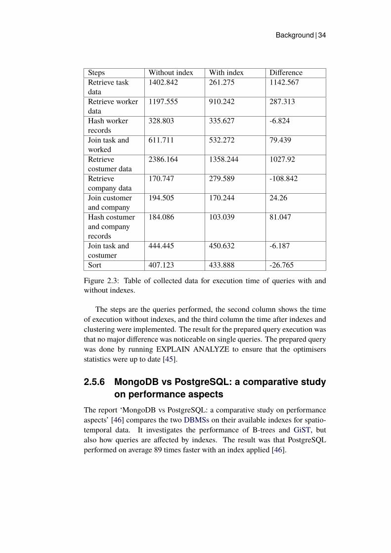
Background | 34

Steps Without index With index DifferenceRetrieve taskdata

1402.842 261.275 1142.567

Retrieve workerdata

1197.555 910.242 287.313

Hash workerrecords

328.803 335.627 -6.824

Join task andworked

611.711 532.272 79.439

Retrievecostumer data

2386.164 1358.244 1027.92

Retrievecompany data

170.747 279.589 -108.842

Join customerand company

194.505 170.244 24.26

Hash costumerand companyrecords

184.086 103.039 81.047

Join task andcostumer

444.445 450.632 -6.187

Sort 407.123 433.888 -26.765

Figure 2.3: Table of collected data for execution time of queries with andwithout indexes.

The steps are the queries performed, the second column shows the timeof execution without indexes, and the third column the time after indexes andclustering were implemented. The result for the prepared query execution wasthat no major difference was noticeable on single queries. The prepared querywas done by running EXPLAIN ANALYZE to ensure that the optimisersstatistics were up to date [45].

2.5.6 MongoDB vs PostgreSQL: a comparative studyon performance aspects

The report ‘MongoDB vs PostgreSQL: a comparative study on performanceaspects’ [46] compares the two DBMSs on their available indexes for spatio-temporal data. It investigates the performance of B-trees and GiST, butalso how queries are affected by indexes. The result was that PostgreSQLperformed on average 89 times faster with an index applied [46].

Background | 35

2.5.7 ComparingOracle andPostgreSQL, performanceand optimization

In the report ‘Comparing Oracle and PostgreSQL, performance and optimi-zation’ [47] the optimisation strategies between theOracleDBMS and Postgre-SQL were compared. This was done using benchmarks with a strategy ofadding column-based indexes to improve query execution. The result showedthat PostgreSQL can improve up to 91% with indexes, which means that it ismore sensitive to optimisation and shows better performance with them. Byonly adding primary and foreign keys the performance was improved by 38%and by adding indexes it was improved by 88% [47].

2.5.8 Space-partitioning Trees in PostgreSQL:Realization and Performance

This report [48] focuses on comparing different implementations of SP-GiSTindexes compared to B+-trees and tries. The SP-GiSTs was implementedwith PostgreSQL was extended to include prefixes and regular expressionmatches, as well as a generic incremental NN search (nearest-neighboursearch). The result showed that a disk based SP-GiST trie performed twoorders of magnitudes better than a B+-tree when it comes to regular expressionmatch searches, while a disk based SP-GiST kd-tree performed more than300% better for a point match than a trie. A disk based suffix tree wasalso implemented for substring match purposes and it performed around threeorders of magnitude better than the existing technique (text scan) at the timeof this report. These implementations were made based on using differentSP-GiST operators, which the report describes as external methods to supportdifferent types of queries.

The SP-GiST trie implementation was compared to the B+-tree in thecontext of text string data, while the SP-GiST kd-tree and PMR quadtree wascompared to R-trees in the context of point and line segment data, respectively.The suffix tree was compared to sequential scanning as there is was no othermethod to support substring matches.

The result shows that a disk based SP-GiST trie performs two orders ofmagnitudes better than a B+-tree when it comes to regular expression matchsearches this was due to how B+-trees are sensitive to where single characterwildcards appear. A wildcard is used with the character ’?’. It retrievesmultiple data sets of a string for example: ?ove = cove, love, dove, etc. Thereason for the result was because the B+-tree used the wildcard in the search,

Background | 36

so if the wildcard appears in the first character then a full table search has to bemade, it explores all the avenues without filtering. The trie on the other handuses non-wildcard characters in the search for filtering.

In this report experimenting, the trie had better search performance thanthe B+-tree when it came to exact match, around 150% better, it also scaledbetter than the B+-tree. For prefix matches the B+-tree outperformed the trie,this was due to the inherent nature of having the keys sorted in the leaf nodes.Which allows the tree to answer prefixmatch queries very efficiently. For exactmatches the B+-tree scales better as well, this is due to how the trie consistsof more nodes and more node splits than the B+-tree.

Kd-tree andR-tree comparisonwas done over a two-dimensional point dataset. The kd-tree performed 300% better than the R-tree when it came to pointsearch and 125% better when it came to range search, although the R-tree hasbetter insertion time and better index size. This is due to how the kd-tree hasa node size (bucket size) of one and every insertion causes a node split. Thisleads to the number of nodes being very large and the clustering technique thatSP-GiST uses to reduce the tree page height costs the index page utilisation.

PMR quadtree in comparison to R-tree for indexing was done on line-segment data sets. The R-tree had better insertion and search performance.

The nearest neighbour search for the kd-tree and the point quadtree wasbetter than for the trie. This is due to how the trie performs the NN searchcharacter by character while for the kd-tree and the point quadtree the NNsearch is based on partitions.

Method | 37

Chapter 3

Method

This chapter describes the research methods and methods used for the testingof optimisation methods. The first section describes the methodologies usedfor the research and how they were used for the project. The sub-questions forthe project are then presented as well as the research approach.

3.1 Research methodsThis section describes the chosen researchmethods and why they were chosen.

3.1.1 Quantitative and qualitative methodsThese two methods are typically applied to projects that are either numericalor non-numerical. Onemethod needs to be chosen to showwhat the research isbased on. Quantitative research verifies or falsifies what is being tested or builtbased on variables that can be measured with quantifications. These methodsneed to use large data sets and use statistics to make the research project valid.Qualitative research on the other hand is used to try and discern meanings todevelop theories for a conclusion. This method uses smaller data sets that aretrustworthy enough to reach a reliable result [49].

Using a qualitativemethod often has the purpose of creating an understand-ing of why things are the way they are. While quantitative methods is aresearch approach that is an objective, formal and systematic process that oftenuses empirical data. It often describes, tests, and examines cause and effect inrelationships by using a deductive process. The difference between qualitativeand quantitative in that sense is that the qualitative approach develops atheory inductively. Other differences can be seen in the sampling of data.

Method | 38

Qualitative methods often choose data sets that are small and selective, whilethe quantitative approach uses large and random data. The purpose of therandom collection of data is to be able to draw general conclusions [50].

3.1.2 Inductive and deductive approachThe inductive approach is used to formulate theories by using explanationsfrom observation. Data is usually collected with qualitative methods andby analysing the data to provide explanations for it, to understand what ishappening. The result is based on experiences and needs to contain enoughdata to explain the phenomenon [49].

The deductive approach is used to verify or falsify a hypothesis, it is mostcommonly used with a quantitative approach. The hypothesis needs to usemeasurable terms and explain the variables measured, as well as express theexpected result. The result from this approach is a generalisation that is basedon the collected data, and the explanation of how variables are related tounderstanding what is happening [49].

The purpose of the inductive approach is to allow findings from frequent,dominant, or significant themes to be found in raw data without putting manyrestrictions on it [51]. Like, for example, when using a deductive approachthe restrictions of the wording formulating the hypotheses can cause the keythemes of the research left invisible or obscured. Therefore the inductiveapproach is better suited to describe the actual effects, not just the plannedeffects. Other purposes of the inductive approach are, to establish clear linksbetween the objectives and the findings from the raw data, and develop a theoryabout the underlying structure that the data shows. In conclusion, the inductiveapproach aims to question the core meanings there are for the research area.This should then be presented by describing the most important themes [51].

3.1.3 SubquestionsThe research question posed in chapter one is "how do indexing and queryoptimisation affect response time for a PostgreSQL database?". To explainwhat this means the question can be divided into sub-questions.

• What methods of indexing are there and what are their use cases?

• How does query optimisation work and how can queries be optimised?

• What is the overlap between indexing and query optimisation?

Method | 39

• How does indexing, the query optimiser, and query tuning compare toeach other?

3.2 Applied methods and research processThis section explains why the methods were chosen, as well as how they areapplied for this thesis by describing the process.

3.2.1 The chosen methodsThe methods chosen for this project is the qualitative and quantitative methodwith an inductive approach.

Finding information for the background and literature has to be donequalitatively as some information is harder to find than others. Making surethat the information is reliable is of higher priority than collecting a largequantity of it. It is also suitable as there are some aspects of the research fieldthat are more explored than others, which means that the sample data in somefields are smaller than others. This is not a big deal in qualitative research aslong as the data is reliable enough and relevant.

The quantitative method is chosen for the experiment. The experimentdeals with a large set of data - although in a specific case - and is performedsimilarly to a laboratory experiment. Such as by including specified variablesto measure, that are measured in a specific environment and with specifiedtools and scripts.

The inductive approach is chosen partly because of the qualitative method,but also because of the purpose of the project. The goal is to observe thebehaviour of indexing and query optimisation to reach an understanding ofwhat is happening. Which matches the purpose of an inductive approach well.Especially when there is no hypothesis and due to the delimitations that restrictthe amount of generalisation that can be made. The theories are formulatedfrom the inductive result are then tested with the quantitative method.

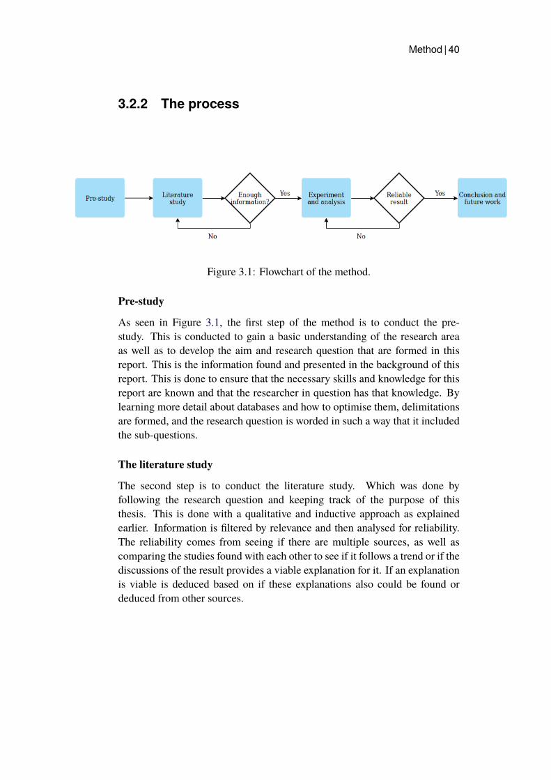
Method | 40

3.2.2 The process

Figure 3.1: Flowchart of the method.

Pre-study

As seen in Figure 3.1, the first step of the method is to conduct the pre-study. This is conducted to gain a basic understanding of the research areaas well as to develop the aim and research question that are formed in thisreport. This is the information found and presented in the background of thisreport. This is done to ensure that the necessary skills and knowledge for thisreport are known and that the researcher in question has that knowledge. Bylearning more detail about databases and how to optimise them, delimitationsare formed, and the research question is worded in such a way that it includedthe sub-questions.

The literature study

The second step is to conduct the literature study. Which was done byfollowing the research question and keeping track of the purpose of thisthesis. This is done with a qualitative and inductive approach as explainedearlier. Information is filtered by relevance and then analysed for reliability.The reliability comes from seeing if there are multiple sources, as well ascomparing the studies found with each other to see if it follows a trend or if thediscussions of the result provides a viable explanation for it. If an explanationis viable is deduced based on if these explanations also could be found ordeduced from other sources.

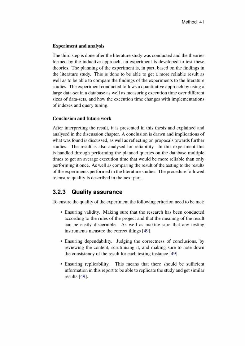
Method | 41

Experiment and analysis

The third step is done after the literature study was conducted and the theoriesformed by the inductive approach, an experiment is developed to test thesetheories. The planning of the experiment is, in part, based on the findings inthe literature study. This is done to be able to get a more reliable result aswell as to be able to compare the findings of the experiments to the literaturestudies. The experiment conducted follows a quantitative approach by using alarge data-set in a database as well as measuring execution time over differentsizes of data-sets, and how the execution time changes with implementationsof indexes and query tuning.

Conclusion and future work

After interpreting the result, it is presented in this thesis and explained andanalysed in the discussion chapter. A conclusion is drawn and implications ofwhat was found is discussed, as well as reflecting on proposals towards furtherstudies. The result is also analysed for reliability. In this experiment thisis handled through performing the planned queries on the database multipletimes to get an average execution time that would be more reliable than onlyperforming it once. As well as comparing the result of the testing to the resultsof the experiments performed in the literature studies. The procedure followedto ensure quality is described in the next part.

3.2.3 Quality assuranceTo ensure the quality of the experiment the following criterion need to be met:

• Ensuring validity. Making sure that the research has been conductedaccording to the rules of the project and that the meaning of the resultcan be easily discernible. As well as making sure that any testinginstruments measure the correct things [49].

• Ensuring dependability. Judging the correctness of conclusions, byreviewing the content, scrutinising it, and making sure to note downthe consistency of the result for each testing instance [49].

• Ensuring replicability. This means that there should be sufficientinformation in this report to be able to replicate the study and get similarresults [49].

Experiment | 42

Chapter 4

Experiment

This chapter goes into detail about the experiment performed for this project.It tells of the hardware and software used, the database design and queriesperformed. The improved queries can be seen in a section below. The databaseschema, and the index design can be found in the appendixes A and C at theend of this report. The details in this chapter should be sufficient enough toensure replicability.

4.1 Experiment designThis section describes under what hardware conditions the experiment wasconducted, as well as what software was used. It then moves onto describinghow the experiment was conducted.

4.1.1 HardwareThe following list presents the relevant hardware used to run the databaseenvironment, for the purpose of replicability of the experiment:

• Motherboard: ROG STRIX X99 gaming

• Random Access Memory (RAM):Corsair Vengeance LED DDR4, 4x8GB, 3400MHz

• CPU:Intel core i7-6850K, 3.6 GHz, 15MB Cache

• SSD: Kingston A400 SSD, 960 GB, 500MB/s read and 450MB/s write

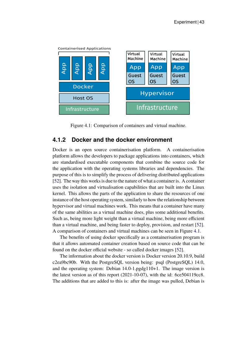
Experiment | 43

Figure 4.1: Comparison of containers and virtual machine.

4.1.2 Docker and the docker environmentDocker is an open source containerisation platform. A containerisationplatform allows the developers to package applications into containers, whichare standardised executable components that combine the source code forthe application with the operating systems libraries and dependencies. Thepurpose of this is to simplify the process of delivering distributed applications[52]. Theway this works is due to the nature of what a container is. A containeruses the isolation and virtualisation capabilities that are built into the Linuxkernel. This allows the parts of the application to share the resources of oneinstance of the host operating system, similarly to how the relationship betweenhypervisor and virtual machines work. This means that a container have manyof the same abilities as a virtual machine does, plus some additional benefits.Such as, being more light weight than a virtual machine, being more efficientthan a virtual machine, and being faster to deploy, provision, and restart [52].A comparison of containers and virtual machines can be seen in Figure 4.1.

The benefits of using docker specifically as a containerisation program isthat it allows automated container creation based on source code that can befound on the docker official website - so called docker images [52].

The information about the docker version is Docker version 20.10.9, buildc2ea9bc90b. With the PostgreSQL version being: psql (PostgreSQL) 14.0,and the operating system: Debian 14.0-1.pgdg110+1. The image version isthe latest version as of this report (2021-10-07), with the id: 6ce504119cc8.The additions that are added to this is: after the image was pulled, Debian is

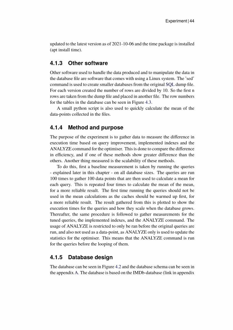
Experiment | 44

updated to the latest version as of 2021-10-06 and the time package is installed(apt install time).

4.1.3 Other softwareOther software used to handle the data produced and to manipulate the data inthe database file are software that comes with using a Linux system. The ’sed’command is used to create smaller databases from the original SQL dump file.For each version created the number of rows are divided by 10. So the first nrows are taken from the dump file and placed in another file. The row numbersfor the tables in the database can be seen in Figure 4.3.

A small python script is also used to quickly calculate the mean of thedata-points collected in the files.

4.1.4 Method and purposeThe purpose of the experiment is to gather data to measure the difference inexecution time based on query improvement, implemented indexes and theANALYZE command for the optimiser. This is done to compare the differencein efficiency, and if one of these methods show greater difference than theothers. Another thing measured is the scalability of these methods.

To do this, first a baseline measurement is taken by running the queries- explained later in this chapter - on all database sizes. The queries are run100 times to gather 100 data points that are then used to calculate a mean foreach query. This is repeated four times to calculate the mean of the mean,for a more reliable result. The first time running the queries should not beused in the mean calculations as the caches should be warmed up first, fora more reliable result. The result gathered from this is plotted to show theexecution times for the queries and how they scale when the database grows.Thereafter, the same procedure is followed to gather measurements for thetuned queries, the implemented indexes, and the ANALYZE command. Theusage of ANALYZE is restricted to only be ran before the original queries arerun, and also not used as a data-point, as ANALYZE only is used to update thestatistics for the optimiser. This means that the ANALYZE command is runfor the queries before the looping of them.

4.1.5 Database designThe database can be seen in Figure 4.2 and the database schema can be seen inthe appendix A. The database is based on the IMDb-database (link in appendix

Experiment | 45

F, which is a database filled with movies, games, tv-shows and other media.It contains information about people who have worked in the media, and howit is rated. The ratings are collected from users on the IMDb website. As thefigure shows, the database only has six tables, with a couple of attributes ineach table. The person table contains the person_id which is just a string ofcharacters to identify the row in the table - and is also the primary key. It alsocontains the surname and last name of the person, their date of birth, and deathdate - which is null if the person is still alive. This table has a one-to-manyrelationship with the crew table as one person can be multiple crew members.The crew table has a title_id - which is the id of the media the crewmemberworked on. The person_id to link to who the person is, a category - which isthe title of their work, i.e actor, director, writer, etc - and job. From lookingat the data in the database file the job column is mostly null values, with theexception for producers who have a repeat of ’producer’, and writers whichhave what they write - poem, play, book - and the title of it in a string.

The next group of tables is the ones that contain information about themedia in the database. The akas table is an overview of the media in thedatabase, it contains the basic information about the media such as the title,the region it was produced in, what language it contains, what type it is - showsIMDb display, original, alternative or null. What attributes it has - informationabout the title, mostly null - and a boolean value for if the title is an originaltitle or not. This then gets further divided into an episodes table, that showsinformation about the episodes in a show, i.e the episode number and seasonnumber. More information about the titles can be found in the titles table. Itshowswhat type ofmedia it is, the original and the primary title of themedia, ifit is adult rated, when it premiered, when it ended (mainly for shows), how longthe runtime for the media is, as well as what genres the media is in. The genrecolumn contains a string of all the genres the media belongs to. The titles tablealso contains the primary key, which is on the title_id column. The last table isthe ratings table, which contains the average rating for the title and how manyvotes it has received, it also has a primary key on the title_id column. Thus,there is a one-to-one relationship between titles and ratings, a one-to-manyrelationship between titles and akas, and a one-to-many relationship betweentitles and episodes.

It is important to note that the database does not contain any foreign keys,the only key constraints that exist are the primary keys that can be seen inFigure 4.2.

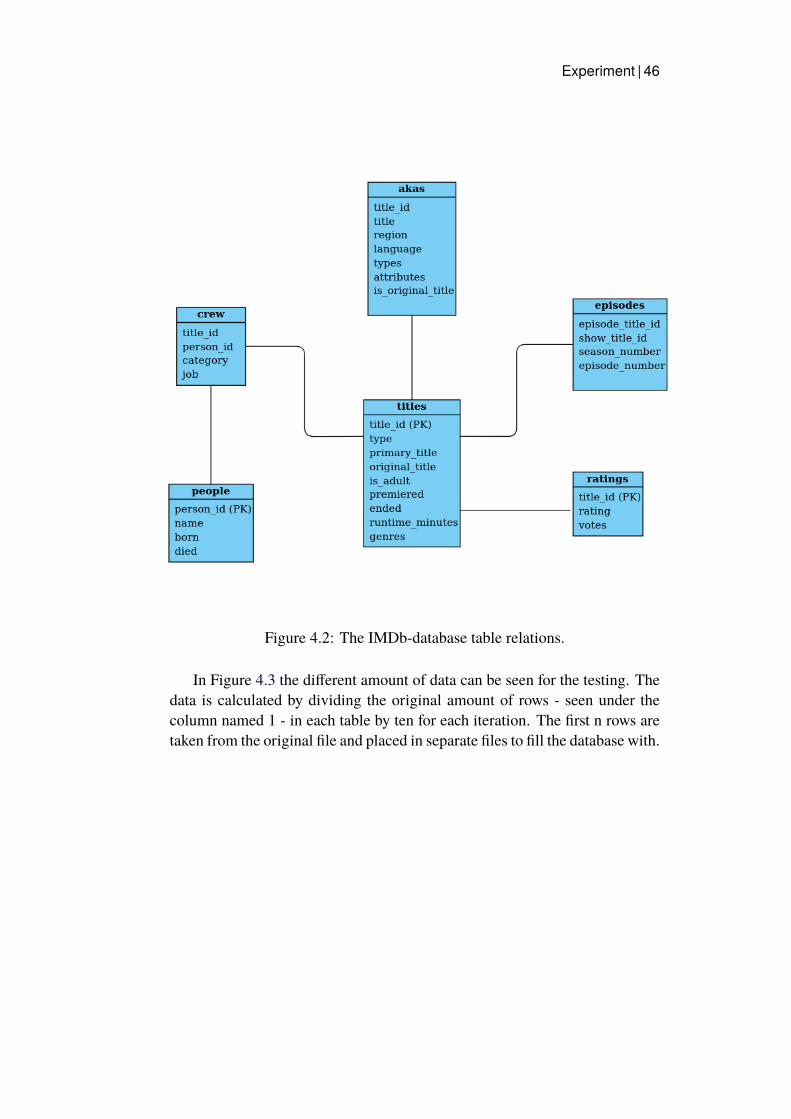
Experiment | 46

Figure 4.2: The IMDb-database table relations.

In Figure 4.3 the different amount of data can be seen for the testing. Thedata is calculated by dividing the original amount of rows - seen under thecolumn named 1 - in each table by ten for each iteration. The first n rows aretaken from the original file and placed in separate files to fill the database with.

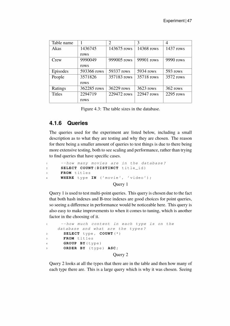
Experiment | 47

Table name 1 2 3 4Akas 1436745

rows143675 rows 14368 rows 1437 rows

Crew 9990049rows

999005 rows 99901 rows 9990 rows

Episodes 593366 rows 59337 rows 5934 rows 593 rowsPeople 3571826

rows357183 rows 35718 rows 3572 rows

Ratings 362285 rows 36229 rows 3623 rows 362 rowsTitles 2294719

rows229472 rows 22947 rows 2295 rows

Figure 4.3: The table sizes in the database.

4.1.6 QueriesThe queries used for the experiment are listed below, including a smalldescription as to what they are testing and why they are chosen. The reasonfor there being a smaller amount of queries to test things is due to there beingmore extensive testing, both to see scaling and performance, rather than tryingto find queries that have specific cases.

1 --how many movies are in the database ?2 SELECT COUNT ( DISTINCT title_id )3 FROM titles4 WHERE type IN (’movie ’, ’video ’);

Query 1

Query 1 is used to test multi-point queries. This query is chosen due to the factthat both hash indexes and B-tree indexes are good choices for point queries,so seeing a difference in performance would be noticeable here. This query isalso easy to make improvements to when it comes to tuning, which is anotherfactor in the choosing of it.

1 --how much content in each type is on thedatabase and what are the types ?

2 SELECT type , COUNT (*)3 FROM titles4 GROUP BY ( type )5 ORDER BY ( type ) ASC ;

Query 2

Query 2 looks at all the types that there are in the table and then how many ofeach type there are. This is a large query which is why it was chosen. Seeing

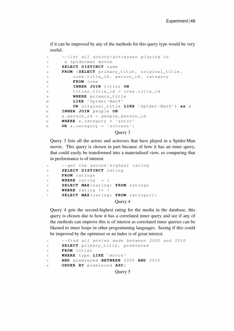
Experiment | 48

if it can be improved by any of the methods for this query type would be veryuseful.

1 -- list all actors / actresses playing in2 a spiderman movie3 SELECT DISTINCT name4 FROM ( SELECT primary_title , original_title ,5 crew . title_id , person_id , category6 FROM crew7 INNER JOIN titles ON8 titles . title_id = crew . title_id9 WHERE primary_title

10 LIKE ’Spider - Man %’11 OR original_title LIKE ’Spider - Man %’) as a12 INNER JOIN people ON13 a. person_id = people . person_id14 WHERE a. category = ’actor ’15 OR a. category = ’ actress ’;

Query 3

Query 3 lists all the actors and actresses that have played in a Spider-Manmovie. This query is chosen in part because of how it has an inner query,that could easily be transformed into a materialised view, so comparing thatin performance is of interest.

1 --get the second - highest rating2 SELECT DISTINCT rating3 FROM ratings4 WHERE rating = (5 SELECT MAX ( rating ) FROM ratings6 WHERE rating != (7 SELECT MAX ( rating ) FROM ratings ));

Query 4

Query 4 gets the second-highest rating for the media in the database, thisquery is chosen due to how it has a correlated inner query and see if any ofthe methods can improve this is of interest as correlated inner queries can belikened to inner loops in other programming languages. Seeing if this couldbe improved by the optimiser or an index is of great interest.

1 -- find all movies made between 2000 and 20102 SELECT primary_title , premiered3 FROM titles4 WHERE type LIKE ’movie ’5 AND premiered BETWEEN 2000 AND 20106 ORDER BY premiered ASC ;

Query 5

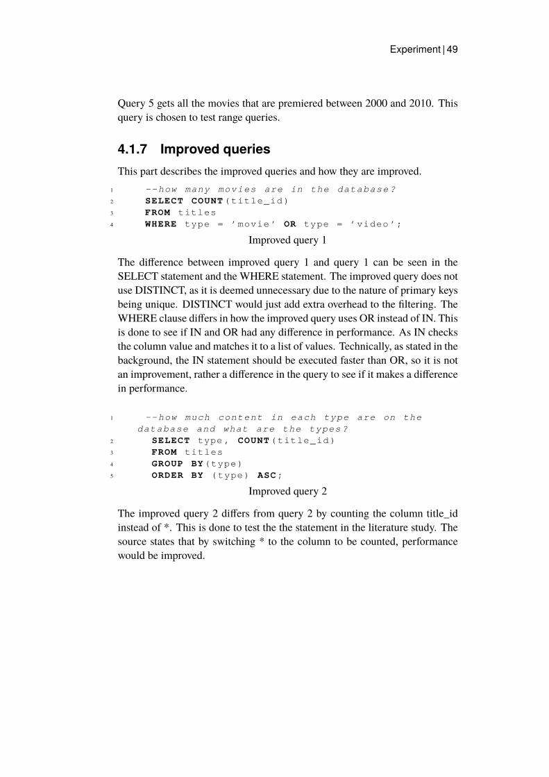
Experiment | 49

Query 5 gets all the movies that are premiered between 2000 and 2010. Thisquery is chosen to test range queries.

4.1.7 Improved queriesThis part describes the improved queries and how they are improved.

1 --how many movies are in the database ?2 SELECT COUNT ( title_id )3 FROM titles4 WHERE type = ’movie ’ OR type = ’video ’;

Improved query 1

The difference between improved query 1 and query 1 can be seen in theSELECT statement and the WHERE statement. The improved query does notuse DISTINCT, as it is deemed unnecessary due to the nature of primary keysbeing unique. DISTINCT would just add extra overhead to the filtering. TheWHERE clause differs in how the improved query uses OR instead of IN. Thisis done to see if IN and OR had any difference in performance. As IN checksthe column value and matches it to a list of values. Technically, as stated in thebackground, the IN statement should be executed faster than OR, so it is notan improvement, rather a difference in the query to see if it makes a differencein performance.

1 --how much content in each type are on thedatabase and what are the types ?

2 SELECT type , COUNT ( title_id )3 FROM titles4 GROUP BY ( type )5 ORDER BY ( type ) ASC ;

Improved query 2

The improved query 2 differs from query 2 by counting the column title_idinstead of *. This is done to test the the statement in the literature study. Thesource states that by switching * to the column to be counted, performancewould be improved.

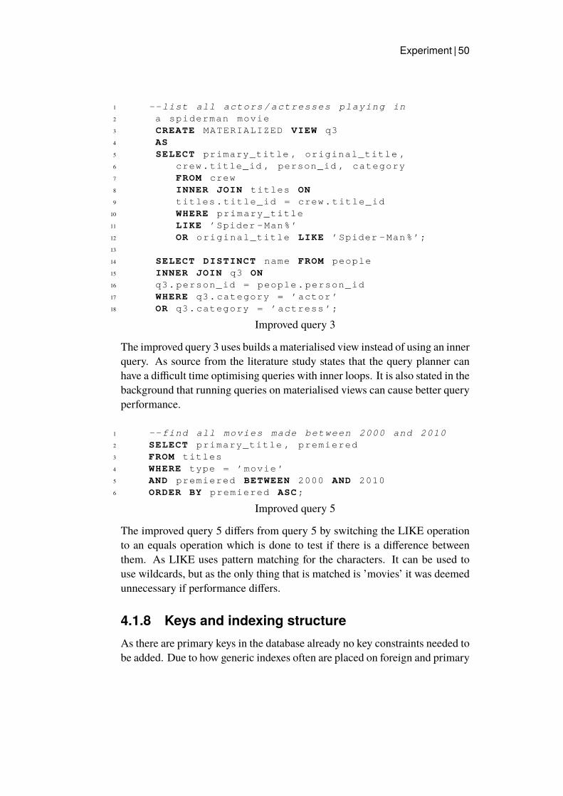
Experiment | 50

1 -- list all actors / actresses playing in2 a spiderman movie3 CREATE MATERIALIZED VIEW q34 AS5 SELECT primary_title , original_title ,6 crew . title_id , person_id , category7 FROM crew8 INNER JOIN titles ON9 titles . title_id = crew . title_id

10 WHERE primary_title11 LIKE ’Spider - Man %’12 OR original_title LIKE ’Spider - Man %’;13

14 SELECT DISTINCT name FROM people15 INNER JOIN q3 ON16 q3. person_id = people . person_id17 WHERE q3. category = ’actor ’18 OR q3. category = ’ actress ’;

Improved query 3

The improved query 3 uses builds a materialised view instead of using an innerquery. As source from the literature study states that the query planner canhave a difficult time optimising queries with inner loops. It is also stated in thebackground that running queries on materialised views can cause better queryperformance.

1 -- find all movies made between 2000 and 20102 SELECT primary_title , premiered3 FROM titles4 WHERE type = ’movie ’5 AND premiered BETWEEN 2000 AND 20106 ORDER BY premiered ASC ;

Improved query 5

The improved query 5 differs from query 5 by switching the LIKE operationto an equals operation which is done to test if there is a difference betweenthem. As LIKE uses pattern matching for the characters. It can be used touse wildcards, but as the only thing that is matched is ’movies’ it was deemedunnecessary if performance differs.

4.1.8 Keys and indexing structureAs there are primary keys in the database already no key constraints needed tobe added. Due to how generic indexes often are placed on foreign and primary

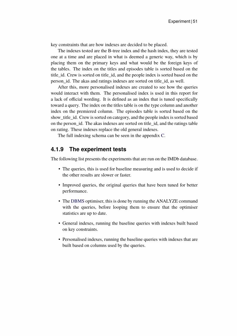
Experiment | 51

key constraints that are how indexes are decided to be placed.The indexes tested are the B-tree index and the hash index, they are tested

one at a time and are placed in what is deemed a generic way, which is byplacing them on the primary keys and what would be the foreign keys ofthe tables. The index on the titles and episodes table is sorted based on thetitle_id. Crew is sorted on title_id, and the people index is sorted based on theperson_id. The akas and ratings indexes are sorted on title_id, as well.

After this, more personalised indexes are created to see how the querieswould interact with them. The personalised index is used in this report fora lack of official wording. It is defined as an index that is tuned specificallytoward a query. The index on the titles table is on the type column and anotherindex on the premiered column. The episodes table is sorted based on theshow_title_id. Crew is sorted on category, and the people index is sorted basedon the person_id. The akas indexes are sorted on title_id, and the ratings tableon rating. These indexes replace the old general indexes.

The full indexing schema can be seen in the appendix C.

4.1.9 The experiment testsThe following list presents the experiments that are run on the IMDb database.

• The queries, this is used for baseline measuring and is used to decide ifthe other results are slower or faster.

• Improved queries, the original queries that have been tuned for betterperformance.

• The DBMS optimiser, this is done by running the ANALYZE commandwith the queries, before looping them to ensure that the optimiserstatistics are up to date.

• General indexes, running the baseline queries with indexes built basedon key constraints.

• Personalised indexes, running the baseline queries with indexes that arebuilt based on columns used by the queries.

Results and Analysis | 52

Chapter 5

Results and Analysis

This chapter summarises the result of the literature study, as well as presentsthe result from the experiment.

5.1 Literature study resultThis section describes the results from the literature study, and can also beseen as a summary of the main points of the Related works section.

5.1.1 TheoryIn the report ’Database performance tuning and query optimization’ [42]the main take-away points are that indexing can be the solution to manyperformance issues, but maintaining an index can cause overhead whenupdating tables. It can also cause CPU and I/O usage to increase whichalso increases the cost of writing data to disk [42]. The book ’Databasetuning principles, experiments, and troubleshooting techniques [43] furtherdevelops on this. First, it describes how a database administrator should thinkto improve a database with a three-step technique:

• Think globally, fix locally: Creating indexes can be a good solution asit can be cheaper than creating more disk space.

• Partitioning break bottlenecks: a local fix to breaking bottlenecks is tocreate indexes.

• Start-up costs are high, running cost is low: improving execution timeoften costs memory or processing power.

Results and Analysis | 53

The book then continues to describe how queries can be divided up into types,and what indexes suit which query type. The query types are described as:

• Point queries return one record or parts of a record based on an equalityselection.

• Multi-point queries return several records based on an equality selection.

• Range queries return a set of records whose values are within an interval.

• Prefix match queries are queries that use AND and LIKE statements, tomatch strings or sets of characters.

• Extremal queries are queries that obtain a set of records that return theminimum or maximum of attribute values.

• Ordering queries use the ORDER BY statement.

• Grouping queries use the GROUP BY statement.

• Join queries are queries that links two or more tables. There are differenttypes of join queries. For joins that use an equality statement (equijoins),the optimisation process is simpler, for join queries that are not equijoinsthe system will try to execute the select statement before joining. Thisis due to non-equijoins often needing to do full table scans, even whenthere is an index present.

B-tree indexes are in particular good for range, prefix match, partial match,point, multipoint, general join, and ordering queries. Clustering B-trees aregood for getting rid of the ORDER BY statement, due to the ordering nature ofB-trees in combination with physical storage. And for non-clustering indexes,covering all the attributes necessary for a query is the best way to use them, asthen it is possible for the DBMS to use an index-only scan. Another type ofindex is the composite index, whose use-cases are mainly to ensure minimaltable accesses for queries that use many of the key attributes in the index.Although, there can become an issue with updates, as this type of index usemany attributes for its key, the chance of the index having to update when thetable does is higher. The major tip from this book is that indexes should beavoided on smaller tables, dense indexes should be used on critical queries tomake use of the index-only scan, and building an index is dependent on if thetime saved in execution time is larger than the cost of updating the index [43].

Some methods for improving queries are getting rid of the * and insteadusing the column name in operations. Make sure that the HAVING clause is

Results and Analysis | 54

executed after restricting the data with the SELECT statements. As well asby minimising the number of subquery blocks that are in a nested query [42].Query tuning should be considered before implementing indexes, as insertingindexes can have harmful global effects. In comparison, rewriting a query canonly have positive effects, if done correctly [43]. Tips for rewriting queriesare:

• Do not use DISTINCT unnecessarily as it creates an overhead due tosorting.

• Avoid subqueries as much as possible, as many systems do not handlethem well.

• Complicated correlation sub-queries can often execute in an inefficientway and should be rewritten.

• The use of temporaries can cause operations to be executed in a sub-optimal manner, but it can also help with subverting the need of usingan ORDER BY statement.

• Do not use HAVING statements if a WHERE statement is enough.

• Study the idiosyncrasies of the system. Some systems might not useindexes when there is an OR statement involved, to circumvent this aunion could be used.

• They state that the ordering of tables in the FROM statement can affectthe order of joins, especially if more than five tables are used.

• The use of views as it can lead to writing inefficient queries.

[43]The book ’PostgreSQL query optimization: the ultimate guide to building

efficient queries’ [21] continues on building the theory for creating optimisedqueries. The book begins by stating that a database application has manyparts, optimising one of them might not improve global performance. Andalso, that PostgreSQL has one of the best query optimisers in the industry, sodeclarative queries should be used. Theway the planner works is by combiningthe primary metrics such as CPU cycles and I/O accesses to a single cost unitthat is used for comparison of plans. Some inaccuracies of the optimiser aremainly due to the stored histograms not being able to produce intermediateresults, cost estimates being imprecise, and that heuristics might cut a plan tooearly to see if it really was not optimal [21].

Results and Analysis | 55

A query can access data in different ways. The main ways are full tablescan, index-only scan, and index access. For smaller values of selectivity,index access is preferable, as it is faster than a full table scan. This also meansthat if selectivity is high, using a full table scan is preferable. But the bestoption is to use an index-only scan if the query allows it. Although this isentirely dependent on the index used [21].

The book then describes short and long queries and how they can be tuned.Short queries benefit from using restrictive indexes and are most efficient withunique indexes, as these have fewer values to go through. Things to keep inmind when using short queries are that column transformations make it sothat an index search cannot be performed on the transformed attribute. LIKEstatements also do not utilise indexes, so they should also be avoided and caninstead be replaced by equivalent OR statements. Some tips for indexing onthe other hand are that indexes should not be used when the table is small, orif the majority of the rows in a table is needed to execute a query, or a columntransformation is used. A tip to force a query to use an index is to use theORDER BY operation [21].

The way to optimise long queries is by avoiding multiple full table scansand reducing the size of the result as soon as possible. Indexes are not neededhere and should not be used. Another tip is that hash join is most likelythe better algorithm for joining long queries. And if GROUP BY is usedby a long query, the filtering needs to be applied first in most cases. Thereare times that GROUP BY can reduce the size of the data-set, but the ruleof thumb is to apply the SELECT statements first for the optimiser. Lastly,set operations can sometimes be used to prompt alternative execution plans.Another tip to improve execution time for queries is to use materialised views,but a materialised view should only be created if the data it is based on doesnot update often. This means that if it is not very critical to have up-to-datedata, the data in the materialised view is read often, and if many queries couldmake use of it [21].

Lastly, multidimensional and spatial searches are discussed. Spatial dataoften require range queries. Which means finding all the data located at acertain distance or closer to a specified point in space. And nearest-neighbourqueries, which is to find a variable number of objects closest to the specifiedpoint. These queries cannot be supported by one-dimensional indexes or evenmultiple indexes, and must instead use special indexes, such as the GiST.

Results and Analysis | 56

5.1.2 Other experimentsIn the report ’Comparison of physical tuning techniques implemented in twoopensource DBMSs’ [44] B-tree indexes and hash indexes were investigatedto see how they affected execution time in two DBMSs. The result showedthat the average time reduced for PostgreSQL with a B-tree index was 67.4%and that the hash index increased execution time for the queries tested [44].This study is complemented by the report ’PostgreSQL database performanceoptimization’ [45], whose result can be seen in Figure 2.3. What can be seen isthat in most cases indexes improved performance, although hashing, joining,retrieving, and sorting sometimes increased execution time. The PostgreSQLoptimiser was also investigated by running the ANALYZE command forqueries, the result was that nomajor difference existed by doing this, comparedto just running the queries [45].

Another study, investigating indexes and how they affect execution time isthe report ’MongoDB vs PostgreSQL: a comparative study on performanceaspects’ [46]. The result showed that PostgreSQL performed on average 89times faster with an index applied [46]. A similar study was done in thereport ’Comparing Oracle and PostgreSQL, performance and optimization’[47] which showed that PostgreSQL can improve up to 91% with indexes andby only adding primary and foreign keys the performance was improved by38% and by adding indexes it was improved by 88% [47].

Lastly, the report ’Space-partitioning Trees in PostgreSQL: Realizationand Performance’ [48] investigated how SP-GiST indexes compared to othertree-based indexes. The result showed that a disk based SP-GiST trie performedtwo orders of magnitudes better than a B+-tree when it comes to regularexpressionmatch searches. The reason for the result was due to the fact that theB+-tree used the wildcard in the search. The trie on the other hand uses non-wildcard characters in the search for filtering. The SP-GiST trie had bettersearch performance than the B+-tree when it came to exact match, around150% better, it also scaled better than the B+-tree. For prefix matches theB+-tree outperformed the SP-GiST trie, this was due to the inherent nature ofhaving the keys sorted in the leaf nodes. Which allows the tree to answer prefixmatch queries very efficiently. For exact matches the B+-tree scales better aswell, this is due to how the SP-GiST trie consists of more nodes and morenode splits than the B+-tree. The SP-GiST kd-tree performed 300% betterthan the R-tree when it came to point search and 125% better when it cameto range search, although the R-tree has better insertion time and better indexsize. This is due to how the kd-tree has a node size (bucket size) of one and

Results and Analysis | 57

every insertion causes a node split. The R-tree had better insertion and searchperformance than the SP-GiST PMR quadtree. Lastly, the nearest neighboursearch for the kd-tree and the point quadtree was better than for the trie. Thisis due to how the trie performs the NN search character by character while forthe kd-tree and the point quadtree the NN search is based on partitions.

5.2 ResultsIn Figure 5.1, Figure 5.2 and, Figure 5.5 the baseline, improved query, andusing the baseline query on the personalised B-tree schema can be seen. Theresult for using the ANALYZE command is omitted due to how it remainedthe same as the query result, the same reason applies to the generic B-tree andHash indexes.

In Figure 5.3 there is also the addition of the generic B-tree and Hashindexes, the optimiser result is once again omitted for the same reason statedbefore.

In Figure 5.4 only the baseline query and the personalised B-tree resultscan be seen. The same reason for omitted results stands as for the firstparagraph. The reason that there is no improved query result, is due to howthat was not tested here.

Detailed results for how the queries were executed, the EXPLAIN output,and more detailed graphs can be seen in the appendix E and D.

5.2.1 Other resultsThe materialised view took less than a minute to build for all data sets. Itshould be noted that different materialised views were tried and some of themtook too long to build in the largest data set. Towards 6 minutes before beingmanually terminated.

Using the ANALYZE command for the optimiser did not show a very bigdifference compared to executing the queries normally. Some queries on somedata sets had the same execution time, others were a millisecond more or less.

The Hash index could not be built for certain columns, due to the nature ofHash structures, so that could not be tested. And for the general indexes, theindex was not used in most queries, which is why that result is omitted.

Further information about the result can be seen in the appendix, bothmoredetailed graphs -in appendix D - for each query executed and the explanationfrom the DBMS, using the EXPLAIN command - in appendix E.

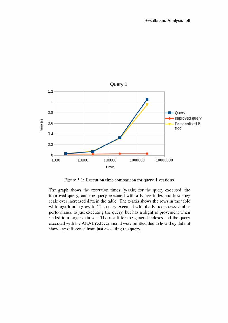
Results and Analysis | 58

Figure 5.1: Execution time comparison for query 1 versions.

The graph shows the execution times (y-axis) for the query executed, theimproved query, and the query executed with a B-tree index and how theyscale over increased data in the table. The x-axis shows the rows in the tablewith logarithmic growth. The query executed with the B-tree shows similarperformance to just executing the query, but has a slight improvement whenscaled to a larger data set. The result for the general indexes and the queryexecuted with the ANALYZE command were omitted due to how they did notshow any difference from just executing the query.

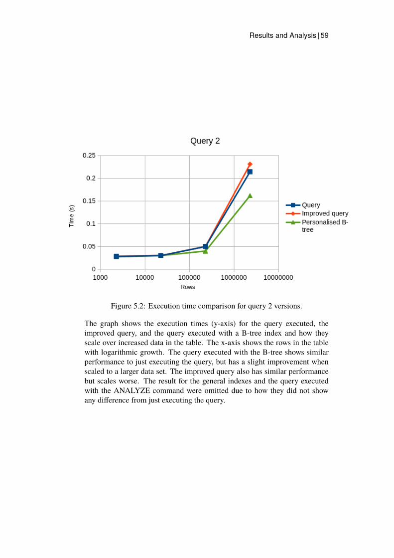
Results and Analysis | 59

Figure 5.2: Execution time comparison for query 2 versions.

The graph shows the execution times (y-axis) for the query executed, theimproved query, and the query executed with a B-tree index and how theyscale over increased data in the table. The x-axis shows the rows in the tablewith logarithmic growth. The query executed with the B-tree shows similarperformance to just executing the query, but has a slight improvement whenscaled to a larger data set. The improved query also has similar performancebut scales worse. The result for the general indexes and the query executedwith the ANALYZE command were omitted due to how they did not showany difference from just executing the query.

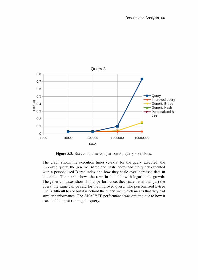
Results and Analysis | 60

Figure 5.3: Execution time comparison for query 3 versions.

The graph shows the execution times (y-axis) for the query executed, theimproved query, the generic B-tree and hash index, and the query executedwith a personalised B-tree index and how they scale over increased data inthe table. The x-axis shows the rows in the table with logarithmic growth.The generic indexes show similar performance, they scale better than just thequery, the same can be said for the improved query. The personalised B-treeline is difficult to see but it is behind the query line, which means that they hadsimilar performance. The ANALYZE performance was omitted due to how itexecuted like just running the query.

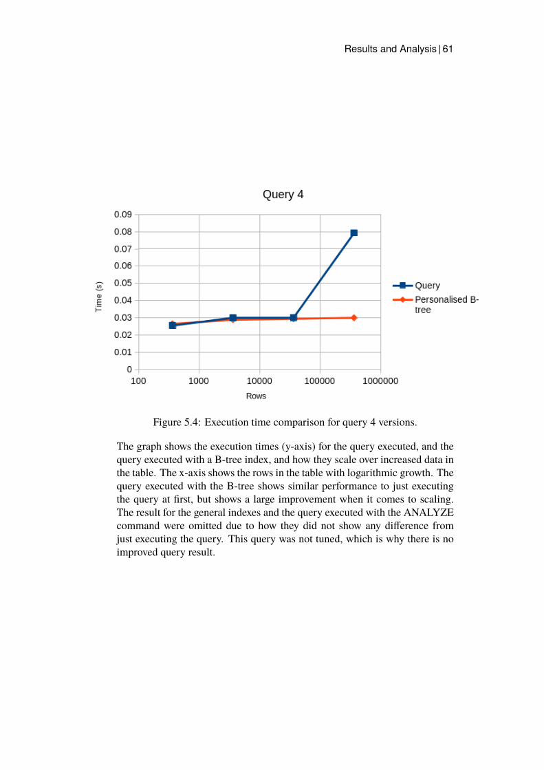
Results and Analysis | 61

Figure 5.4: Execution time comparison for query 4 versions.

The graph shows the execution times (y-axis) for the query executed, and thequery executed with a B-tree index, and how they scale over increased data inthe table. The x-axis shows the rows in the table with logarithmic growth. Thequery executed with the B-tree shows similar performance to just executingthe query at first, but shows a large improvement when it comes to scaling.The result for the general indexes and the query executed with the ANALYZEcommand were omitted due to how they did not show any difference fromjust executing the query. This query was not tuned, which is why there is noimproved query result.

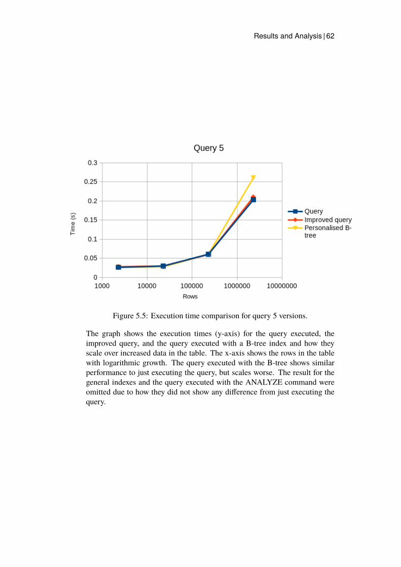
Results and Analysis | 62

Figure 5.5: Execution time comparison for query 5 versions.

The graph shows the execution times (y-axis) for the query executed, theimproved query, and the query executed with a B-tree index and how theyscale over increased data in the table. The x-axis shows the rows in the tablewith logarithmic growth. The query executed with the B-tree shows similarperformance to just executing the query, but scales worse. The result for thegeneral indexes and the query executed with the ANALYZE command wereomitted due to how they did not show any difference from just executing thequery.

Discussion | 63

Chapter 6

Discussion

This chapter discusses and provides explanations for the result in the experi-ment by using the information provided in the background as well as theappendix. It compares the result to the literature studies and analyses thereliability and validity of the result. It also discusses the problems faced duringthe thesis, how they were solved and what problems could not be solved. Itbrings up the sources of errors to consider as well as the limitations of the resultand reiterates what sustainability and ethical effects this result may have.

6.1 The resultThis section describes the result of the experiment, combines it with theEXPLAIN output to shine light onto why the result looks like it does, andcompares it to other the result from the literature study.

As mentioned in the background, EXPLAIN is used to provide an outputof the query plan that the query planner in the DBMS has provided. The outputis read bottom-up, and it uses an abstract measurement

Query 1

As can be seen in Figure 5.1, the query and the query executed on the B-treehave similar execution times, but the B-tree query scales slightly better. Theimproved query on the other hand shows a very big improvement. To bettersee the result see Figure D.6 in the appendix D. The difference between thenormal query and the improved query is the usage of DISTINCT, and IN andOR. From the EXPLAIN output file (in the appendix E), it shows that it filtersthe IN statement first for any strings that contain any of ’movie’ or ’video’, as

Discussion | 64

it contains it as listed values. Then a sequential scan is performed on titles.In comparison, the improved query filters the text using OR statements. Aparallel sequential scan is run with two workers, which means that it mostlikely uses one worker each to scan for either movie or video at the same time.The OR statement seemed to have allowed the planner to use two workersinstead of one, which could have led to better performance, or the lack ofDISTINCT could have done this further tests would be needed to be sure ofwhat the cause was.

The query using the B-tree index functions similarly to how just runningthe query works. What differs is how the query uses the B-tree index byperforming a bitmap index scan followed by a bitmap heap scan rather thana sequential scan. The index it uses has the column type on the table titles asthe indexing column, which means that it has a faster time finding where thecorrect rows are placed on file, but it still needs to access the data, which iswhy the bitmap heap scan also is performed.

The Hash index could not be implemented on the types column, mainlydue to the nature of Hash structures and how they do not work well with manyentries that use the same hash key. The result for the generalised indexes wasalso omitted from the result as the query did not use the index.

Query 2

In Figure 5.2 the result for executing the query, the improved query, and thequery on the B-tree index can be seen. What is most notable is that theimproved query was not improved at all. The query differs from the originalquery by using SELECT(title_id) instead of SELECT(*). The difference inperformance is minimal, yet the sources from the literature study stated thatchanging the * should improve performance. The query performed on theindex scaled better.

The EXPLAIN output shows that for the query first a parallel sequentialscan is performed, then it is partially hashed based on type, this is then sortedon the type as well, and then finallymerged into the result. The improved queryshows the same output as the normal query, which means that technically bothof them should have the same performance. This can be noted as until thelargest data-set was used, the performance was incredibly similar, and for thelargest data-set, the performance only differs by less than amillisecond. Whichcould be a source of error, potentially due to caching. Or it could be an effectof having implemented a materialised view, which might be hogging somememory.

Discussion | 65

The query performed on the B-tree index uses the index with the typescolumn as the indexing column. It first performs an index-only scan, thengroups the types, and finally merges the result. It does this with two workersas well. This explains why this is faster than performing the query withoutindexes, as an index-only scan is faster than a sequential scan. It also does notperform any type of sorting as the B-tree already has the data sorted whichalso saves time.

As stated before, the Hash index could not be implemented on the typescolumn, mainly due to the nature of Hash structures and how they do notwork well with many entries that use the same Hash key. The result for thegeneralised indexes was also omitted from the result as the query did not usethe index.

Query 3

As Figure 5.3 states, the query executed on the generic B-tree and Hashindexes have the same execution times, and they both show slight improvementcompared to executing the querywithout an index. The tuned query also showsslight improvement when it comes to scaling. The other B-tree index has thesame performance as just executing the query. The improved query showsa big improvement compared to the other tests. It should also be noted thatbuilding the materialised view for the improved query took less than a minute.

The EXPLAIN output is quite long but can be summarised as the following.The query uses an index condition on the primary key for the people table, itthen does an index scan using the primary key on people. After this, the queryfilters the movie titles and gathers the titles that are searched for. This is donewith a parallel sequential scan on titles and then hashed. Another parallelsequential scan is run on crew, the result is then hashed and then a hash join isapplied to form the result of the nested loop. This is then sorted by name andthe result is merged.

The improved query on the other hand uses an index scan on the primarykey for the people table, it uses the cached key for the materialised view(as it also contains person_id) for memoisation purposes. The set is thenfiltered on the crew conditions and a nested sequential scan is performed onthe materialised view. The result is then sorted.

The query on the generic B-tree and Hash index shows similar outputs.They both do an index scan based on the person_id column, they then filterthe category on the crew table and use the index condition for title_id (as it isa primary key for titles). They then both do a parallel sequential scan on titles

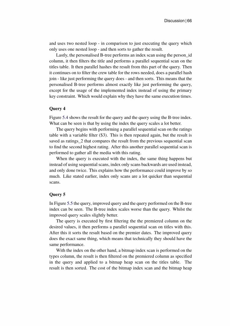
Discussion | 66

and uses two nested loop - in comparison to just executing the query whichonly uses one nested loop - and then sorts to gather the result.

Lastly, the personalised B-tree performs an index scan using the person_idcolumn, it then filters the title and performs a parallel sequential scan on thetitles table. It then parallel hashes the result from this part of the query. Thenit continues on to filter the crew table for the rows needed, does a parallel hashjoin - like just performing the query does - and then sorts. This means that thepersonalised B-tree performs almost exactly like just performing the query,except for the usage of the implemented index instead of using the primarykey constraint. Which would explain why they have the same execution times.

Query 4

Figure 5.4 shows the result for the query and the query using the B-tree index.What can be seen is that by using the index the query scales a lot better.

The query begins with performing a parallel sequential scan on the ratingstable with a variable filter ($3). This is then repeated again, but the result issaved as ratings_2 that compares the result from the previous sequential scanto find the second highest rating. After this another parallel sequential scan isperformed to gather all the media with this rating.

When the query is executed with the index, the same thing happens butinstead of using sequential scans, index only scans backwards are used instead,and only done twice. This explains how the performance could improve by somuch. Like stated earlier, index only scans are a lot quicker than sequentialscans.

Query 5

In Figure 5.5 the query, improved query and the query performed on the B-treeindex can be seen. The B-tree index scales worse than the query. Whilst theimproved query scales slightly better.

The query is executed by first filtering the the premiered column on thedesired values, it then performs a parallel sequential scan on titles with this.After this it sorts the result based on the premier dates. The improved querydoes the exact same thing, which means that technically they should have thesame performance.

With the index on the other hand, a bitmap index scan is performed on thetypes column, the result is then filtered on the premiered column as specifiedin the query and applied to a bitmap heap scan on the titles table. Theresult is then sorted. The cost of the bitmap index scan and the bitmap heap

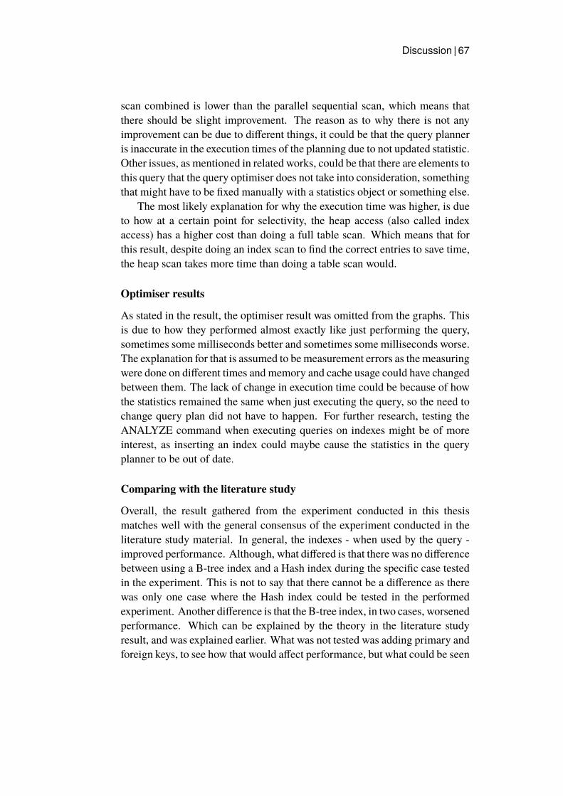
Discussion | 67

scan combined is lower than the parallel sequential scan, which means thatthere should be slight improvement. The reason as to why there is not anyimprovement can be due to different things, it could be that the query planneris inaccurate in the execution times of the planning due to not updated statistic.Other issues, as mentioned in related works, could be that there are elements tothis query that the query optimiser does not take into consideration, somethingthat might have to be fixed manually with a statistics object or something else.

The most likely explanation for why the execution time was higher, is dueto how at a certain point for selectivity, the heap access (also called indexaccess) has a higher cost than doing a full table scan. Which means that forthis result, despite doing an index scan to find the correct entries to save time,the heap scan takes more time than doing a table scan would.

Optimiser results

As stated in the result, the optimiser result was omitted from the graphs. Thisis due to how they performed almost exactly like just performing the query,sometimes some milliseconds better and sometimes some milliseconds worse.The explanation for that is assumed to be measurement errors as the measuringwere done on different times and memory and cache usage could have changedbetween them. The lack of change in execution time could be because of howthe statistics remained the same when just executing the query, so the need tochange query plan did not have to happen. For further research, testing theANALYZE command when executing queries on indexes might be of moreinterest, as inserting an index could maybe cause the statistics in the queryplanner to be out of date.

Comparing with the literature study

Overall, the result gathered from the experiment conducted in this thesismatches well with the general consensus of the experiment conducted in theliterature study material. In general, the indexes - when used by the query -improved performance. Although, what differed is that there was no differencebetween using a B-tree index and a Hash index during the specific case testedin the experiment. This is not to say that there cannot be a difference as therewas only one case where the Hash index could be tested in the performedexperiment. Another difference is that the B-tree index, in two cases, worsenedperformance. Which can be explained by the theory in the literature studyresult, and was explained earlier. What was not tested was adding primary andforeign keys, to see how that would affect performance, but what could be seen

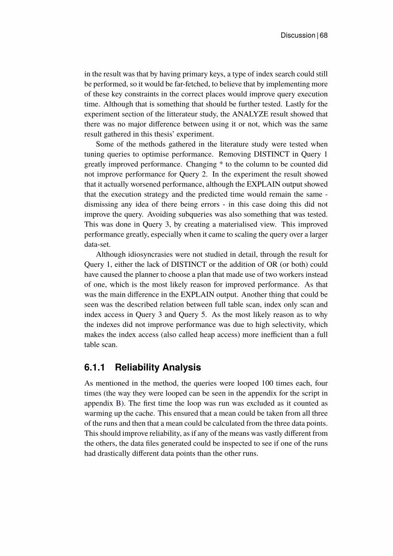
Discussion | 68

in the result was that by having primary keys, a type of index search could stillbe performed, so it would be far-fetched, to believe that by implementing moreof these key constraints in the correct places would improve query executiontime. Although that is something that should be further tested. Lastly for theexperiment section of the litterateur study, the ANALYZE result showed thatthere was no major difference between using it or not, which was the sameresult gathered in this thesis’ experiment.

Some of the methods gathered in the literature study were tested whentuning queries to optimise performance. Removing DISTINCT in Query 1greatly improved performance. Changing * to the column to be counted didnot improve performance for Query 2. In the experiment the result showedthat it actually worsened performance, although the EXPLAIN output showedthat the execution strategy and the predicted time would remain the same -dismissing any idea of there being errors - in this case doing this did notimprove the query. Avoiding subqueries was also something that was tested.This was done in Query 3, by creating a materialised view. This improvedperformance greatly, especially when it came to scaling the query over a largerdata-set.

Although idiosyncrasies were not studied in detail, through the result forQuery 1, either the lack of DISTINCT or the addition of OR (or both) couldhave caused the planner to choose a plan that made use of two workers insteadof one, which is the most likely reason for improved performance. As thatwas the main difference in the EXPLAIN output. Another thing that could beseen was the described relation between full table scan, index only scan andindex access in Query 3 and Query 5. As the most likely reason as to whythe indexes did not improve performance was due to high selectivity, whichmakes the index access (also called heap access) more inefficient than a fulltable scan.

6.1.1 Reliability AnalysisAs mentioned in the method, the queries were looped 100 times each, fourtimes (the way they were looped can be seen in the appendix for the script inappendix B). The first time the loop was run was excluded as it counted aswarming up the cache. This ensured that a mean could be taken from all threeof the runs and then that a mean could be calculated from the three data points.This should improve reliability, as if any of the means was vastly different fromthe others, the data files generated could be inspected to see if one of the runshad drastically different data points than the other runs.

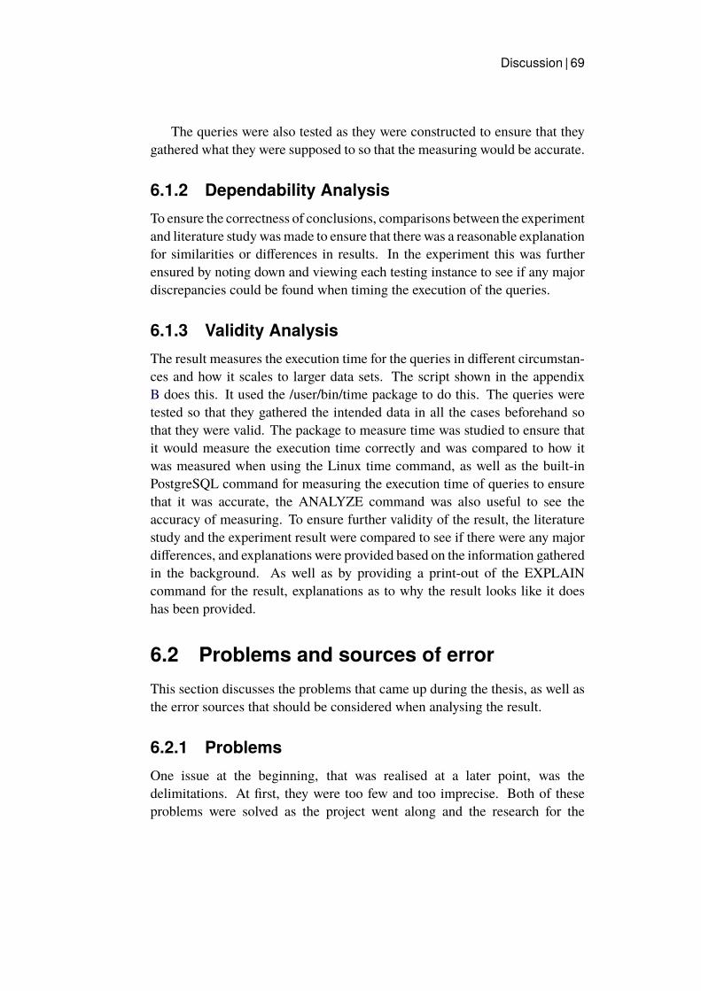
Discussion | 69

The queries were also tested as they were constructed to ensure that theygathered what they were supposed to so that the measuring would be accurate.

6.1.2 Dependability AnalysisTo ensure the correctness of conclusions, comparisons between the experimentand literature studywasmade to ensure that there was a reasonable explanationfor similarities or differences in results. In the experiment this was furtherensured by noting down and viewing each testing instance to see if any majordiscrepancies could be found when timing the execution of the queries.

6.1.3 Validity AnalysisThe result measures the execution time for the queries in different circumstan-ces and how it scales to larger data sets. The script shown in the appendixB does this. It used the /user/bin/time package to do this. The queries weretested so that they gathered the intended data in all the cases beforehand sothat they were valid. The package to measure time was studied to ensure thatit would measure the execution time correctly and was compared to how itwas measured when using the Linux time command, as well as the built-inPostgreSQL command for measuring the execution time of queries to ensurethat it was accurate, the ANALYZE command was also useful to see theaccuracy of measuring. To ensure further validity of the result, the literaturestudy and the experiment result were compared to see if there were any majordifferences, and explanations were provided based on the information gatheredin the background. As well as by providing a print-out of the EXPLAINcommand for the result, explanations as to why the result looks like it doeshas been provided.

6.2 Problems and sources of errorThis section discusses the problems that came up during the thesis, as well asthe error sources that should be considered when analysing the result.

6.2.1 ProblemsOne issue at the beginning, that was realised at a later point, was thedelimitations. At first, they were too few and too imprecise. Both of theseproblems were solved as the project went along and the research for the

Discussion | 70

background and the literature study was found and analysed. The backgroundshowed the extent of the area of database optimisation, which caused moredelimitations to be formed, and the literature study showed how other studiedformulated problems and described the problem area which made it easier toform the research questions for this thesis.

Another issue found during this study was that there are many differentindexes for PostgreSQL, as mentioned in the background. The issue was thatthe information found about them pointed towards their main use case is fora specific type of data - spatio-temporal - or specific types of operations -nearest neighbour search, find coordinates within an area, etc. Due to thetime constraints of this thesis, there was no time to experiment with thesetypes of indexes which meant that they were also put as a delimitation forthe experiment. Although, a couple of research papers were found within thearea of spatio-temporal indexing, in which a few of them contained tests donewith PostgreSQL. One of these reports was more relevant than the others andwas then put in the literature study result. This was done to have some relevantinformation about the use cases of one of the indexes, and also how it comparesto other indexes used in the same problem area.

More problems were found when the experiment was being planned. First,there was no documentation of the data in the database, therefore, some ofthe data was looked over to check what each attribute actually meant. Aswell as to see if there were any key constraints. At first, the constraints werenot found at all, because they were at the end of the file. When they werefound a plan was made to test to see if they could be changed to includemore foreign keys. Due to the nature of the data in the database, and that thedata was decided to be split for the multiple versions of the database, makingforeign keys was difficult, and had to be foregone entirely. Which meant thatonly the original key constraints were used for the database and the indexesimplemented. Another issue found was some issues with query tuning, sincethat was somewhat of a novel concept, formulating better queries was a bitdifficult and in some cases almost impossible. This can be seen in the case ofQuery 4, which was not tuned due to a lack of knowledge.

6.2.2 Sources of errorOne major source of an error discovered was the lack of ability to clear thecache between query runs. In reality, a database would not be running the samequeries on loop, whichmeans that the cachemay not have the data needed at alltimes. There was not a way to do this, due to the nature of Docker only having

Discussion | 71

a readable operating system environment, which is why the exact times shouldbe taken with a grain of salt. Clearing the cache between queries would notsimulate a real database, but would insteadmeasure the worst-case benchmark,which would mean that most likely in a real-life scenario the benchmark wouldbe better than measured. Which means that the result would be more accurate.As mentioned earlier, there were also issues with query tuning, which meansthat the queries might not have been tuned very well, which means that theresult might not show the extent of how the query tuning can improve executiontime.

Another smaller source of error is that the running of tests happened duringdifferent days, and times of days (query and improved query on one day, andindex and optimiser on another). This could cause errors in that cache andmemory performance can differ, which could lead to minor execution timedifferences.

It should also be noted that for Query 3 the two smaller data sets did notreturn any result, so the scaling could be inaccurate for them. And for Query 4,the ratings table is a lot smaller than the other tables, which means that scalingdifferences, in the beginning, could be a lot smaller than for the other results.It would be of interest to have a larger ratings table to see if that reasoning iscorrect or not.

6.3 LimitationsThere are some limitations to the result that areworthmentioning. One of themis what was brought up in the background. As mentioned, a database is oftennot a standalone product, it most often is connected to some sort of applicationas an interface of sorts, and a server. The result of this thesis does not take intoaccount how application or server issues play into efficiency. Neither doesit test hardware, to see how that affects efficiency. Both are limitations thatshould be taken into consideration when optimising a database.

Another limitation is the fact that other PostgreSQL indexes than the B-tree and Hash index could not be tested. The Hash index could not be tested inall cases either. This means that the extent of improvement that indexes haveon a database could not be accurately measured. Although it could be arguedthat by PostgreSQL using the B-tree as the standard indexing structure, therecould be something in that the B-tree most often is suitable for indexing.

Discussion | 72

6.4 SustainabilityAs mentioned in the introduction, optimising a database system has anenvironmental effect as it reduces the resources a database uses. Shorterresponse time and efficient use of hardware lead to lessening the total computingtime and could reduce the wear on hardware as well as a reduction in energyusage. And an ethical problem that is related to database efficiency, is thepotential that people more easily can manage to compile data from differentdata sets. This can then be presented or used to discern information that cancause privacy issues.

Conclusions and Future work | 73

Chapter 7

Conclusions and Future work

This chapter summarises the result and the information discussed in thediscussion chapter, as well as answering the research questions, and sub-questions posed.

7.1 ConclusionThe purpose of this thesis was to investigate how indexing and query optimisationaffect the response time for a PostgreSQL database, with the purpose offurthering research in the area, as well as providing information for databaseadministrators and students alike. As one of the aims was to provide coursematerial for database courses.

To summarise the findings of the experiment and the literature study, theresearch question and the subquestions are answered below.

7.1.1 Answering the subquestionsThe subquestions posed for this thesis is the following:

1. What methods of indexing are there and what are their use cases?

2. How does query optimisation work and how can queries be optimised?

3. What is the overlap between indexing and query optimisation?

4. How does indexing, the query optimiser, and query tuning compare toeach other?

Conclusions and Future work | 74

Subquestion 1

As discovered in the background and literature study, there are many typesof indexes in PostgreSQL. The methods of implementing indexes differdepending on if they are primary or secondary indexes. As in PostgreSQL,only secondary indexes are used, the focus will lay there to answer thisquestion. The method to implement indexes is to look at the queries, analysetheir frequency, and what type of queries they are. As well as looking atthe table to see what type of data there is on there and how often it getsupdated. Depending on the data types and index structure that should bechosen, this also depends on the types of queries that are supposed to usethe index. Thereafter it can be determined what should go into the index ifit should be sparse or dense. And also if the index needs to index all data ina table, if it does not a partial index can be used. If the query uses multipletables, or other columns than what is indexed, determine if a composite indexcan be used.

The use-cases of indexes aremainly determined bywhat indexing structuresare used. In most cases, the type of query or data type can determine whatindex should be used. For example, as mentioned in the background, theHash index is suitable for point, and multi-point queries. Which B-trees alsoare good for but are also extended to include range queries, prefix matches,and ordering queries. SP-GiST, GiST, GIN and BRIN are mostly used forimplementing special data-types into a database. In the literature study SP-GiSTwas described to mainly be used for spatio-temporal data, and dependingon how these indexes are implemented - i.e what data structures are used -they can be useful for different types of queries. This result recommendedtheir implementations of SP-GiST trie for regular expression matches, exactmatches B+-trees for prefix match queries, the SP-GiST kd-tree for pointsearch and range searches, but if insertion and index size is of critical nature,the R-tree works better. This also is the reason to use an R-tree over a SP-GiSTPMR quadtree. Nearest neighbour searches also benefit from using a kd-treeimplementation.

A generalisation based on the gathered result would be that using a B-treeindex is more versatile and suits more situations than using a hash index wouldbe, but if implemented incorrectly could instead slow down the execution time.Removing DISTINCT from a query where possible makes the scaling of aquery a lot better than using the operation. On smaller data sets (in this thesistables with less than 100 000 rows) rarely show a difference in execution timeno matter if an index is implemented or if a query is tuned.

Conclusions and Future work | 75

Subquestion 2

Query optimisation can be separated into two parts, query tuning, and usingthe query optimiser. The query optimiser is part of the DBMS and workswith statistics over the database, and the query planner to ensure that a goodquery plan is chosen. This is done by looking at specific factors, such as CPUcycles and I/O accesses, combining them to a single unit, and then comparingthis unit between plans. The PostgreSQL optimiser can update the statisticsby running the ANALYZE command for a query, as well as be improved byimplementing supported statistical objects - for multivariate statistics. This isnecessary as there are use cases where the optimiser does not work well, suchas for correlated columns in queries, etc. The query planner optimises a queryby setting up a plan tree, with plan nodes, in which each plan node containsthe cost of planned execution (in the special unit). To not have infinite plans,and ensure that the optimised query is the equivalent of the starting query,heuristics rules are used.

Query tuning on the other hand uses techniques and the skills of the querywriter. It is done by manually rewriting queries, to better make use of thedatabase resources. This is entirely based on the knowledge that the querywriter has about the database and the query language used. As differenttypes of queries benefit from different optimisation techniques. Summarisedtechniques from the literature study result are:

• Do not use DISTINCT unless necessary.

• Avoid subqueries as much as possible, especially correlated subqueries.

• Temporaries can cause execution to be slow, but can also subvert theneed for using ORDER BY operations.

• Do not use HAVING if WHERE is enough.

• Depending on the system, some operations can cause the query to notuse indexes. These idiosyncrasies need to be studied.

• Ordering in the FROM statement can influence the ordering of JOINs,especially if more than five tables are joined.

• The use of views can lead to writing inefficient queries.

• Index-only scans are always faster than full table scans, but index accesscan be slower than full table scans if the selectivity of the query is high.

Conclusions and Future work | 76

• Short queries benefit from using restrictive indexes, especially when theindexes are unique as well.

• Doing a column transformation can cause indexes to not be used.

• ORDER BY can force the query to use an index.

• Long queries, do not benefit from indexes, and instead are optimised byensuring that few full table scans are done. It is also beneficial to reducethe size of the result as soon as possible.

• Materialised views are good for improving execution time if it is notcritical for the query to have fully up-to-date data.

Based on the experiment result, using an OR statement instead of an INoperation could also potentially improve performance, although more testswould be needed to verify that.

Subquestion 3

From the information stated, indexing and queries are incredibly entwined.The purpose of both query optimisation and indexing is to improve efficiency.Although, this can be done in different ways. Indexing can be used for theordering of files, which would be one of the main differences. Anotherdifference is that because of how indexes need to be implemented on thedatabase as an auxiliary structure, query optimisation can be a less invasiveprocedure to use when improving execution time on a sensitive database. Suchas for databases that cannot affordmorememory allocation, or have their tableschanging often. From the experiment, it can also be seen that, in the case of theexperiment, it is only so much an index can do if the query is bad. So queryoptimisation and indexing have areas where they both are entwined to havegood execution time. The query optimiser is always running as well, althoughthe accuracy can be improved by specific operations based on data type, query,and other factors. This means that the optimiser overlap with both indexes andquery tuning.

Subquestion 4

From subquestion 3, it can then be argued to mean that one method cannotbe superior to the others, as something like this cannot be generalised. It alldepends on the situation. How the database looks if the database structurecan change, how much memory is available, and if there is a priority to

Conclusions and Future work | 77

queries. Although, based on the result we can split it up into some cases.Implementing indexes for spatio-temporal data improves execution time forqueries - this should be complemented with seeing how query optimisationaffects it though. B-tree indexes are more well-rounded in their use cases, andfrom the experiment worked really well for improving a correlated subquery.Query tuning worked really well for a nested query (by using a materialisedview), as well as for a large query (selecting many rows in a table) - whichwas also stated in the literature study as long queries benefit more from queryoptimisation than indexes. Based on the literature study result, in cases ofcolumn transformation query optimisation works better. And for short queries,using indexes is more beneficial.

7.1.2 The research questionThe research question summarises the subquestions. Indexing and queryoptimisations affect the response time positively if implemented correctly, ascan be seen, both in the literature study and the experiment conducted for thisthesis report. Although, there are cases where indexes can increase executiontime. In the literature study, this happened during hashing records, retrievingrecords from a specific table, joining certain tables, and sorting. In the caseof the experiment conducted in this thesis: Query 5 (range query) and also, inpart Query 3 (nested join query), which happened due to incorrect usage ofindexes. Tuning queries, on the other hand, had two cases of showing greatperformance improvement, one of them being Query 3 (with the materialisedview) and Query 1 (removing DISTINCT), which concludes that materialisedviews improves the execution time, and scales very well, but needs to beweighed against the cost of creating and maintaining it. The other two casesshowed a lack of improvement, but this most likely was due to a lack of tuningknowledge. The query optimiser (ANALYZE) on the other hand did not affectresponse time majorly. This means that depending on the case response timecan be affected positively or negatively - or not at all - by implementing indexesor query optimisation techniques.

7.2 Future workFor further research, ideas of interest can be seen in the following list.

• Testing more of the different query types that are mentioned in [43], tosee how they interact with indexes, the optimiser, and query tuning.

Conclusions and Future work | 78

• Testing the different statistical elements in the optimiser.

• Have larger data sets and different types of data, to be able to generaliseconclusions.

• See how normalisation affects execution time.

• See how key constraints affect execution time.

• Implement one of the other PostgreSQL indexes, to see how they affectperformance.

• Testing the cost of indexes by using update or remove operations on atable, as well as testing the cost of updating a materialised view. Tobetter understand their use-cases.

This is mainly motivated by filling in the gaps for the limitations of the resultin this thesis. Having this information, and more information in general,would make a stronger case for the conclusions of this thesis. As wellas, further mapping out more information about optimisation techniques ingeneral. As of this thesis, it was somewhat difficult to find other publishedresearch focusing specifically on PostgreSQL and how to optimise a databasewithin it. Complementing this thesis with any of the above suggestionswould contribute to having more detailed and specific information for thePostgreSQL community.

7.3 ReflectionsThis chapter describes some reflections of the works, suggestions towardsothers, what I would change about the works, and the impact of the work done.As well as some other thoughts about the project.

7.3.1 Thoughts about the workDuring the course of this works, I found out and learned a lot more in-depthabout databases, as well as how to conduct a research project. What I alsofound, was a lack of official, or published research about this area in particular.It was difficult to conduct the literature study as most materials were notvery similar to the work being done in this thesis. So my suggestion forothers working within database systems would be to publish more detailedinformation about optimisation techniques and their explanations. I would

Conclusions and Future work | 79

say that doing the pre-study was an integral part of this thesis, so for otherthesis students, I would recommend conducting a pre-study to collect basicknowledge about what information is out there within their research area. Toensure that what they are doing is possible, and within the delimitations.

Some things I would change if I were to redo this work are to summarisethe literature study result before conducting the experiment, as it would havesaved me more time than having to go back and forth in the report to findthe information I need. As well as, when writing, spending that time actuallyformulating and editing as I go, instead of writing the necessary informationand then having to go back and edit large sections at a time. I believe that itwould have been faster if I had spent the time writing it better the first time.This potentially could have given me more time for the experiment, so that Icould have tested more scenarios.

7.3.2 ImpactThe impact of the result of this thesis, I believe is somewhat small on asocio-econimic scale. I think it could have a larger impact on students as itsummarises a lot of information, and test it on a specified database language.Which they then could use for their own learning purposes. I also believethat it could potentially help database administrators that have started workingwith PostgreSQL. I believe that if continued, this research has the potential ofhaving a high impact on the PostgreSQL community in the sense of makingit even more available. This could lead to more people, and companies usingPostgreSQL for their relational databases.

Asmentioned in the discussion and the background, the impact of optimisationcan improve environmental costs. Partly by less usage of hardware leads toless wear, and also software optimisation could lead to needing to upgradehardware less. Another environmental improvement would be that needingless time for execution could lead to less energy usage overall. This could alsobe argued to help companies to keep unnecessary costs down.

REFERENCES | 80

References

[1] R. Elmazri and N. B. Shamkant, The fundamentals of database systems.Pearson, 2016.

[2] H. E. Williams and D. Lane, Web Database Applications withPHP & MySQL. O’Reilly Media, 2002-04-16, [Online]https://www.oreilly.com/library/view/web-database-applications/0596005431/ch01.html, (Accessed: 2021-09-01).

[3] M. Bakni. (2017-08-02) Client-server 3-tier architecture. [Online]https://commons.wikimedia.org/wiki/File:Client-Server_3-tier_architecture_-_en.png, (Accessed: 2021-10-06).

[4] N. Fialkovskaya. (2021-01-08) Speed test. [Online] https://sitechecker.pro/speed-test/, (Accessed: 2021-09-01).

[5] S. O’dea. Average internet connection speed in theus. [Online] https://www.statista.com/statistics/616210/average-internet-connection-speed-in-the-us/, (Accessed: 2021-08-24).

[6] Oracle. What is a database? [Online] https://www.oracle.com/database/what-is-database/, (Accessed: 2021-08-25).

[7] IBM Cloud Education. Relational databases. [Online] https://www.ibm.com/cloud/learn/relational-databases, (Accessed: 2021-09-01).

[8] GeeksforGeeks. (2021-06-28) Dbms set1. [Online] https://www.geeksforgeeks.org/introduction-of-dbms-database-management-system-set-1/, (Accessed:2021-09-17).

[9] Ian. (2016-06-06) What is a database schema? [Online] https://database.guide/what-is-a-database-schema/, (Accessed: 2021-09-17).

REFERENCES | 81

[10] PostgreSQL Global Development Group. Postgresql documentationintroduction. [Online] https://www.postgresql.org/docs/13/intro-whatis.html, (Accessed: 2021-09-03).

[11] ——. Architectural fundamentals. [Online] https://www.postgresql.org/docs/13/tutorial-arch.html, (Accessed: 2021-09-03).

[12] ——. Sql concepts. [Online] https://www.postgresql.org/docs/13/tutorial-concepts.html, (Accessed: 2021-09-03).

[13] ——.Advanced features: foreign keys. [Online] https://www.postgresql.org/docs/13/tutorial-fk.html, (Accessed: 2021-09-03).

[14] ——. Constraints. [Online] https://www.postgresql.org/docs/8.3/ddl-constraints.html#DDL-CONSTRAINTS-FK, (Accessed: 2021-09-17).

[15] PostgreSQL Tutorial. Postgresql tutorial. [Online] https://www.postgresqltutorial.com/, (Accessed: 2021-10-21).

[16] ——. Postgresql like. [Online] https://www.postgresqltutorial.com/postgresql-like/, (Accessed: 2021-10-21).

[17] ——. Postgresql in. [Online] https://www.postgresqltutorial.com/postgresql-in/, (Accessed: 2021-10-21).

[18] ——. Postgresql subquery. [Online] https://www.postgresqltutorial.com/postgresql-subquery/, (Accessed: 2021-10-21).

[19] Geeks for geeks. Sql correlated subqueries. [Online] https://www.geeksforgeeks.org/sql-correlated-subqueries/, (Accessed: 2021-10-21).

[20] PostgreSQL Global Development Group. Views. [Online] https://www.postgresql.org/docs/13/tutorial-views.html, (Accessed: 2021-09-04).

[21] H. Dombrovskaya, B. Novikov, and A. Bailliekova, PostgreSQL queryoptimization: the ultimate guide to building efficient queries. Apress,2021.

[22] PostgreSQL Global Development Group. Materialised views. [Online]https://www.postgresql.org/docs/current/rules-materializedviews.html,(Accessed: 2021-09-04).

REFERENCES | 82

[23] GeeksforGeeks. (2021-09-07) File organization in dbms. [Online] https://www.geeksforgeeks.org/file-organization-in-dbms-set-1/, (Accessed:2021-09-17).

[24] PostgreSQL Global Development Group. Indexes: introduction.[Online] https://www.postgresql.org/docs/13/indexes-intro.html,(Accessed: 2021-09-03).

[25] ——. Index types. [Online] https://www.postgresql.org/docs/13/indexes-types.html, (Accessed: 2021-09-03).

[26] ——. Multicolumn indexes. [Online] https://www.postgresql.org/docs/13/indexes-multicolumn.html, (Accessed: 2021-09-03).

[27] Ta bu shi da yu . (2005-06-17) B-tree index. [Online] https://en.wikipedia.org/wiki/File:Btree_index.PNG, (Accessed: 2021-09-27).

[28] PostgreSQL Global Development Group. Hash indexes. [Online] https://www.postgresql.org/docs/13/hash-intro.html, (Accessed: 2021-09-04).

[29] J. Stolfi. (2009-04-10) Hash table. [Online] https://commons.wikimedia.org/wiki/File:Hash_table_5_0_1_1_1_1_1_LL.svg, (Accessed: 2021-10-06).

[30] PostgreSQL Global Development Group. Gist indexes. [Online] https://www.postgresql.org/docs/13/gist-intro.html, (Accessed: 2021-09-03).

[31] ——. Operator classes and operator families. [Online] https://www.postgresql.org/docs/9.5/indexes-opclass.html, (Accessed: 2021-09-18).

[32] ——. Sp-gist indexes. [Online] https://www.postgresql.org/docs/13/spgist-intro.html, (Accessed: 2021-09-03).

[33] ——. Gin indexes. [Online] https://www.postgresql.org/docs/13/gin-intro.html, (Accessed: 2021-09-03).

[34] ——. Brin indexes. [Online] https://www.postgresql.org/docs/13/brin-intro.html, (Accessed: 2021-09-03).

[35] ——.Combining indexes. [Online] https://www.postgresql.org/docs/13/indexes-bitmap-scans.html, (Accessed: 2021-09-03).

[36] ——. Partial indexes. [Online] https://www.postgresql.org/docs/13/indexes-partial.html, (Accessed: 2021-09-03).

REFERENCES | 83

[37] ——. Index-only scans. [Online] https://www.postgresql.org/docs/13/indexes-index-only-scans.html, (Accessed: 2021-09-03).

[38] ——. Multi-version concurrency control. [Online] https://www.postgresql.org/docs/7.1/mvcc.html, (Accessed: 2021-09-18).

[39] ——. Query planner. [Online] https://www.postgresql.org/docs/13/using-explain.html, (Accessed: 2021-09-04).

[40] ——. Query planner statistics. [Online] https://www.postgresql.org/docs/13/planner-stats.html, (Accessed: 2021-09-04).

[41] ——. Oins and the query planner. [Online] https://www.postgresql.org/docs/13/explicit-joins.html, (Accessed: 2021-09-04).

[42] S. J. Kamatkar, A. Kamble, A. Viloria, L. Hernandez-Fernandez, andE. Garcia, “Database performance tuning and query optimization,” inLecture notes in computer science 10943 - Data mining and big data,2018, pp. 3–11.

[43] D. Sasha and P. Bonnet, Database tuning principles, experiments andtroubleshooting techniques. Morgan Kaufman, 2002.

[44] F. Oyvind, “Comparison of physical tuning techniques implemented intwo open source dbmss,” 2005.

[45] Q. Wang, “Postgresql database performance optimization,” 2011.

[46] A. Makris, K. Tserpes, G. Spiliopoulus, D. Zissis, andD. Anagnostopoulos, “Mongodb vs postgresql: a comparative study onperfomance aspects,” 2020.

[47] P. Martins, P. Tomé, C. Wanzeller, F. A. Sá, and M. Abbasi, “Comparingoracle and postgresql, performance and optimization,” in Trends andapplications in information systems and technologies, vol. II, 2021, pp.3–11.

[48] M. Y. Eltabakh, R. Eltarras, and W. G. Aref, “Space-partitioning treesin postgresql: Realization and performance,” in Proceedings of the 22ndInternational Conference on Data Engineering, 2006, [Online] https://www.cerias.purdue.edu/assets/pdf/bibtex_archive/01617468.pdf,(Accessed: 2021-10-21).

REFERENCES | 84

[49] A. Håkansson, “Portal of research methods and methodologies forresearch projects and degree projects,” in WORLDCOMP’13 - The2013 World Congress in Computer Science, Computer Engineering, andApplied Computing, 2013.

[50] N. B. Nkomo and J. Lihanda, “Qualitative and quantitativemethodology,” 2010-05-21, [Online] https://www.academia.edu/44204575/QUALITATIVE_AND_QUANTITATIVE_METHODOLOGY, (Accessed: 2021-09-21).

[51] D. R. Tomas, “A general inductive approach for analyzing qualitativeevaluation data,” 2006-06, [Online] https://journals.sagepub.com/doi/pdf/10.1177/1098214005283748, (Accessed: 2021-09-21).

[52] IBM Cloud Education. (2021-06-23) Docker. [Online] https://www.ibm.com/cloud/learn/docker, (Accessed: 2021-10-07).

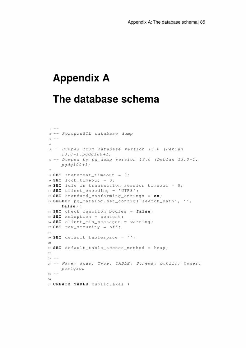
Appendix A: The database schema | 85

Appendix A

The database schema

1 --2 -- PostgreSQL database dump3 --4

5 -- Dumped from database version 13.0 ( Debian13.0 -1. pgdg100 +1)

6 -- Dumped by pg_dump version 13.0 ( Debian 13.0 -1.pgdg100 +1)

7

8 SET statement_timeout = 0;9 SET lock_timeout = 0;

10 SET idle_in_transaction_session_timeout = 0;11 SET client_encoding = ’UTF8 ’;12 SET standard_conforming_strings = on ;13 SELECT pg_catalog . set_config (’ search_path ’, ’’,

false );14 SET check_function_bodies = false ;15 SET xmloption = content ;16 SET client_min_messages = warning ;17 SET row_security = off ;18

19 SET default_tablespace = ’’;20

21 SET default_table_access_method = heap ;22

23 --24 -- Name : akas ; Type : TABLE ; Schema : public ; Owner :

postgres25 --26

27 CREATE TABLE public . akas (

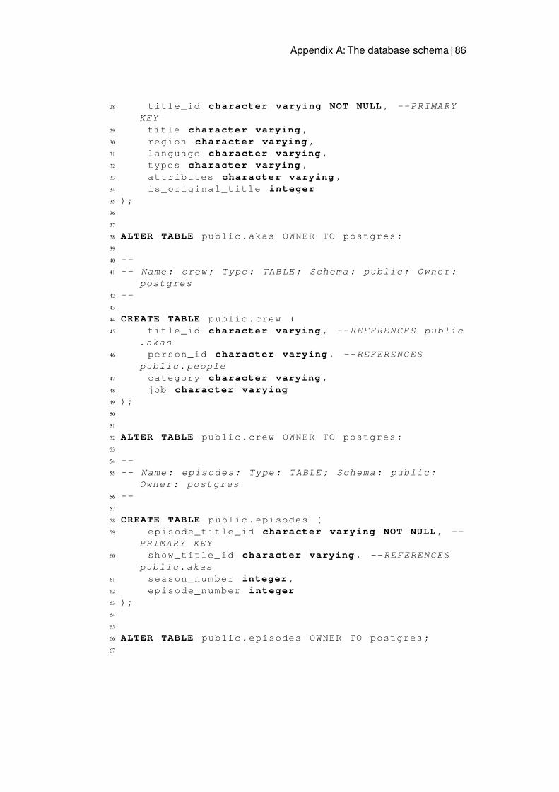
Appendix A: The database schema | 86

28 title_id character varying NOT NULL , -- PRIMARYKEY

29 title character varying ,30 region character varying ,31 language character varying ,32 types character varying ,33 attributes character varying ,34 is_original_title integer35 );36

37

38 ALTER TABLE public . akas OWNER TO postgres ;39

40 --41 -- Name : crew ; Type : TABLE ; Schema : public ; Owner :

postgres42 --43

44 CREATE TABLE public . crew (45 title_id character varying , -- REFERENCES public

. akas46 person_id character varying , -- REFERENCES

public . people47 category character varying ,48 job character varying49 );50

51

52 ALTER TABLE public . crew OWNER TO postgres ;53

54 --55 -- Name : episodes ; Type : TABLE ; Schema : public ;

Owner : postgres56 --57

58 CREATE TABLE public . episodes (59 episode_title_id character varying NOT NULL , --

PRIMARY KEY60 show_title_id character varying , -- REFERENCES

public . akas61 season_number integer ,62 episode_number integer63 );64

65

66 ALTER TABLE public . episodes OWNER TO postgres ;67

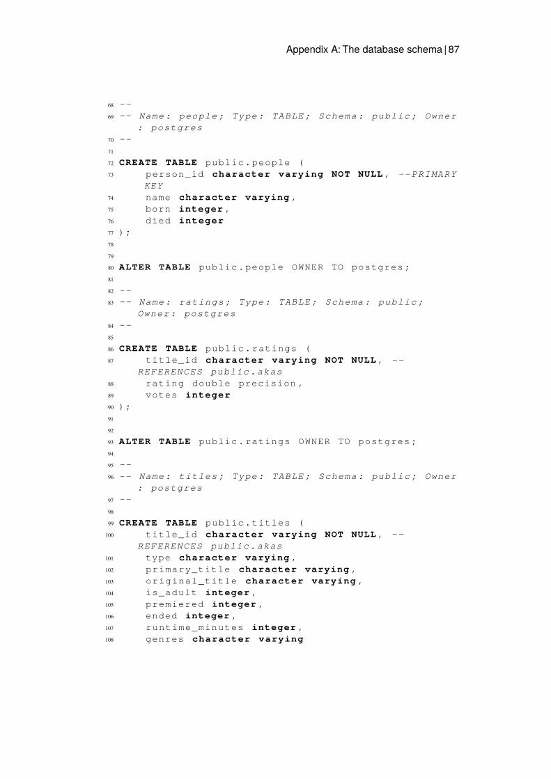
Appendix A: The database schema | 87

68 --69 -- Name : people ; Type : TABLE ; Schema : public ; Owner

: postgres70 --71

72 CREATE TABLE public . people (73 person_id character varying NOT NULL , -- PRIMARY

KEY74 name character varying ,75 born integer ,76 died integer77 );78

79

80 ALTER TABLE public . people OWNER TO postgres ;81

82 --83 -- Name : ratings ; Type : TABLE ; Schema : public ;

Owner : postgres84 --85

86 CREATE TABLE public . ratings (87 title_id character varying NOT NULL , --

REFERENCES public . akas88 rating double precision ,89 votes integer90 );91

92

93 ALTER TABLE public . ratings OWNER TO postgres ;94

95 --96 -- Name : titles ; Type : TABLE ; Schema : public ; Owner

: postgres97 --98

99 CREATE TABLE public . titles (100 title_id character varying NOT NULL , --

REFERENCES public . akas101 type character varying ,102 primary_title character varying ,103 original_title character varying ,104 is_adult integer ,105 premiered integer ,106 ended integer ,107 runtime_minutes integer ,108 genres character varying

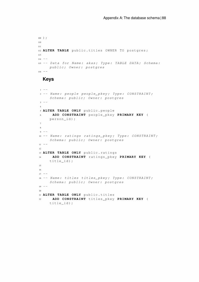
Appendix A: The database schema | 88

109 );110

111

112 ALTER TABLE public . titles OWNER TO postgres ;113

114 --115 -- Data for Name : akas ; Type : TABLE DATA ; Schema :

public ; Owner : postgres116 --

Keys

1 --2 -- Name : people people_pkey ; Type : CONSTRAINT ;

Schema : public ; Owner : postgres3 --4

5 ALTER TABLE ONLY public . people6 ADD CONSTRAINT people_pkey PRIMARY KEY (

person_id );7

8

9 --10 -- Name : ratings ratings_pkey ; Type : CONSTRAINT ;

Schema : public ; Owner : postgres11 --12

13 ALTER TABLE ONLY public . ratings14 ADD CONSTRAINT ratings_pkey PRIMARY KEY (

title_id );15

16

17 --18 -- Name : titles titles_pkey ; Type : CONSTRAINT ;

Schema : public ; Owner : postgres19 --20

21 ALTER TABLE ONLY public . titles22 ADD CONSTRAINT titles_pkey PRIMARY KEY (

title_id );

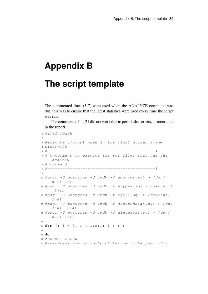
Appendix B: The script template | 89

Appendix B

The script template

The commented lines (5-7) were used when the ANALYZE command wasrun, this was to ensure that the latest statistics were used every time the scriptwas run.

The commented line 21 did not work due to permission errors, asmentionedin the report.

1 #!/ bin / bash2

3 # execute ./ loop1 when in the right docker image4 LIMIT =1005 # -------------------------------------------#6 # Uncomment to execute the sql files that has the

ANALYZE7 # command8 # -------------------------------------------#9

10 # psql -U postgres -d imdb -f amovies . sql > / dev /null 2 >&1

11 # psql -U postgres -d imdb -f atypes . sql > / dev / null2 >&1

12 # psql -U postgres -d imdb -f ajoin . sql > / dev / null2 >&1

13 # psql -U postgres -d imdb -f asecondhigh . sql > / dev/ null 2 >&1

14 # psql -U postgres -d imdb -f ainterval . sql > / dev /null 2 >&1

15

16 for (( i = 0; i < LIMIT ; i++ ));17

18 do19 # FORMAT BELOW20 #/ usr / bin / time -o <outputfile > -a -f %e psql -U <

Appendix B: The script template | 90

username docker > -d < database name in docker > -f<name of query file > > / dev / null 2 >&1

21 #-a -f %e flags has to do with the / usr / bin / timepackage and how it formats time output

22 # > / dev / null 2 >&1 throws the sql output into null ,so it does not show in the terminal

23

24 / usr / bin / time -o movies1 . txt -a -f %e psql -Upostgres -d imdb -f movies . sql > / dev / null 2 >&1

25 / usr / bin / time -o types1 . txt -a -f %e psql -Upostgres -d imdb -f types . sql > / dev / null 2 >&1

26 / usr / bin / time -o join1 . txt -a -f %e psql -Upostgres -d imdb -f join . sql > / dev / null 2 >&1

27 / usr / bin / time -o secondhigh1 . txt -a -f %e psql -Upostgres -d imdb -f secondhigh . sql > / dev / null2 >&1

28 / usr / bin / time -o interval1 . txt -a -f %e psql -Upostgres -d imdb -f interval . sql > / dev / null2 >&1

29

30 # sync && echo 1 > / proc / sys /vm/ drop_caches # dropscache ?

31 done ;32 echo -ne ’\n’

Appendix C: Indexes | 91

Appendix C

Indexes

B-tree indexesThe commented indexes are the generic indexes that were first tested.

1 -- CREATE INDEX titles_b ON public . titles USINGBTREE ( title_id );

2 -- CREATE INDEX akas_b ON public . akas USING BTREE (title_id );

3 -- CREATE INDEX crew_b ON public . crew USING BTREE (title_id );

4 -- CREATE INDEX people_b ON public . people USINGBTREE ( person_id );

5 -- CREATE INDEX ratings_b ON public . ratings USINGBTREE ( title_id );

6 -- CREATE INDEX episodes_b ON public . episodes USINGBTREE ( show_title_id );

7

8 CREATE INDEX titles_b ON public . titles USING BTREE (type );

9 CREATE INDEX titlesprem_b ON public . titles USINGBTREE ( premiered );

10 CREATE INDEX akas_b ON public . akas USING BTREE (title_id );

11 CREATE INDEX crew_b ON public . crew USING BTREE (category );

12 CREATE INDEX people_b ON public . people USING BTREE (person_id );

13 CREATE INDEX ratings_b ON public . ratings USINGBTREE ( rating );

14 CREATE INDEX episodes_b ON public . episodes USINGBTREE ( show_title_id );

Appendix C: Indexes | 92

Hash indexesThe commented indexes are the personalised indexes that could not be generatedfor the large database.

1 CREATE INDEX titles_b ON public . titles USING HASH (title_id );

2 CREATE INDEX akas_b ON public . akas USING HASH (title_id );

3 CREATE INDEX crew_b ON public . crew USING HASH (title_id );

4 CREATE INDEX people_b ON public . people USING HASH (person_id );

5 CREATE INDEX ratings_b ON public . ratings USING HASH( title_id );

6 CREATE INDEX episodes_b ON public . episodes USINGHASH ( show_title_id );

7

8 -- CREATE INDEX titles_b ON public . titles USING HASH( type );

9 -- CREATE INDEX titlesprem_b ON public . titles USINGHASH ( premiered );

10 -- CREATE INDEX akas_b ON public . akas USING HASH (title_id );

11 -- CREATE INDEX crew_b ON public . crew USING HASH (category );

12 -- CREATE INDEX people_b ON public . people USING HASH( person_id );

13 -- CREATE INDEX ratings_b ON public . ratings USINGHASH ( rating );

14 -- CREATE INDEX episodes_b ON public . episodes USINGHASH ( show_title_id );

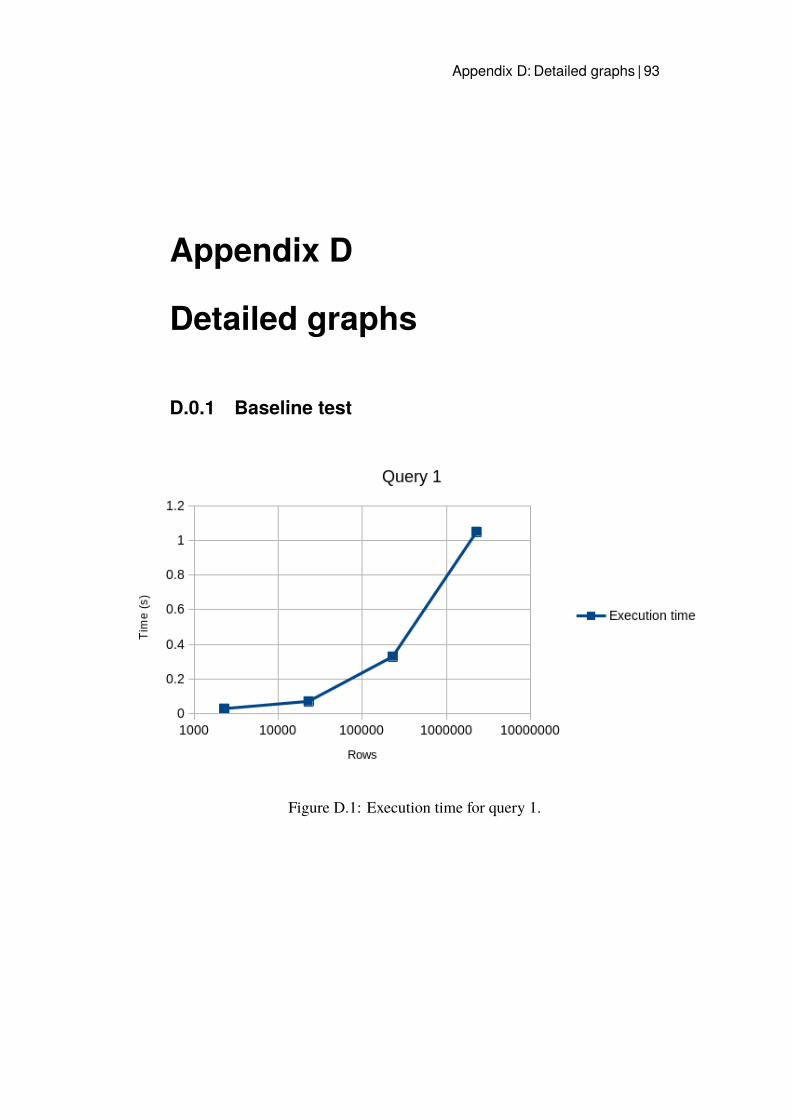
Appendix D: Detailed graphs | 93

Appendix D

Detailed graphs

D.0.1 Baseline test

Figure D.1: Execution time for query 1.

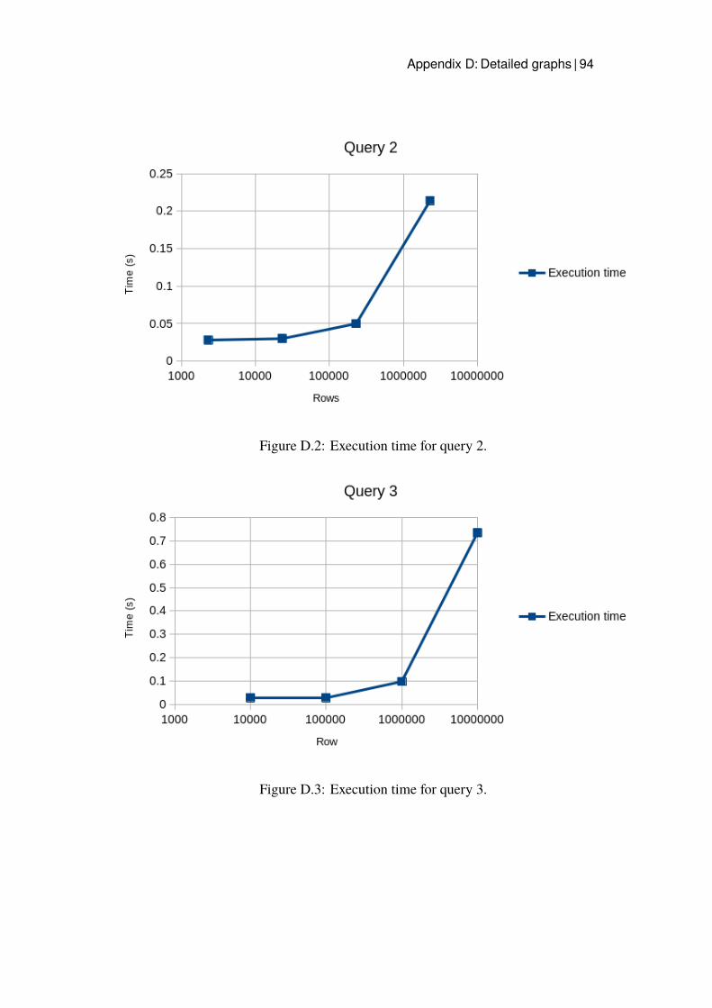
Appendix D: Detailed graphs | 94

Figure D.2: Execution time for query 2.

Figure D.3: Execution time for query 3.

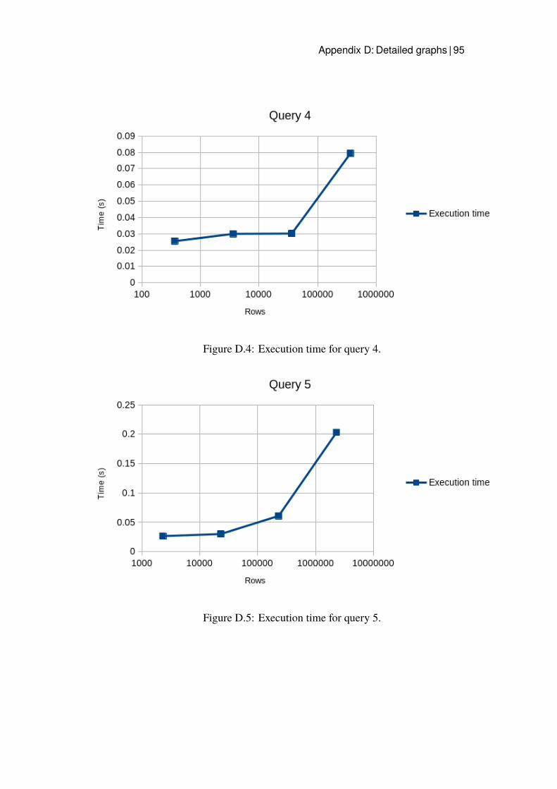
Appendix D: Detailed graphs | 95

Figure D.4: Execution time for query 4.

Figure D.5: Execution time for query 5.

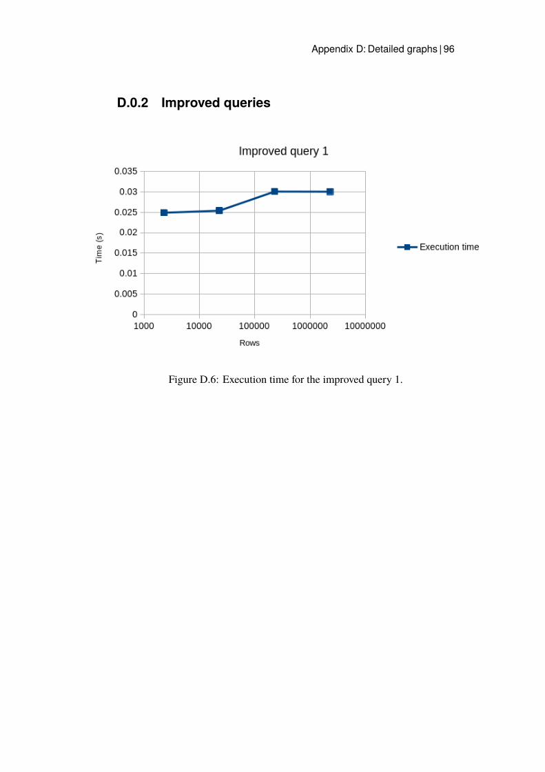
Appendix D: Detailed graphs | 96

D.0.2 Improved queries

Figure D.6: Execution time for the improved query 1.

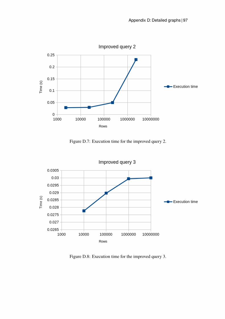
Appendix D: Detailed graphs | 97

Figure D.7: Execution time for the improved query 2.

Figure D.8: Execution time for the improved query 3.

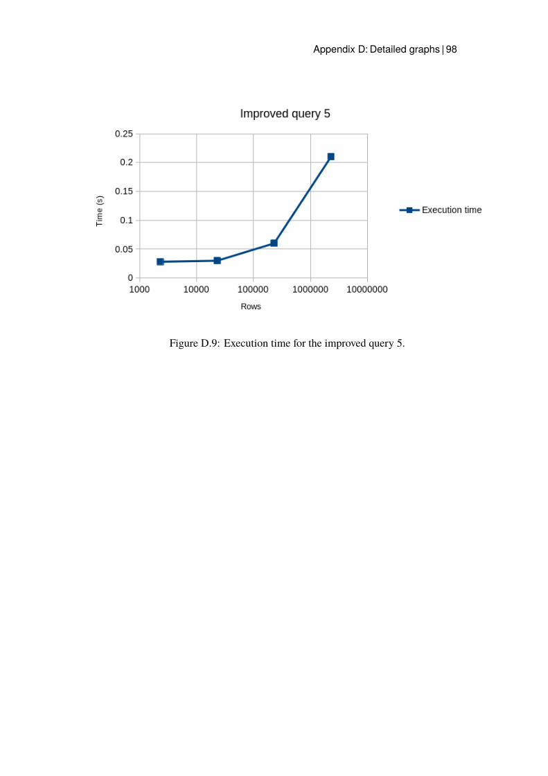
Appendix D: Detailed graphs | 98

Figure D.9: Execution time for the improved query 5.

Appendix D: Detailed graphs | 99

D.0.3 Hash index

Figure D.10: Execution time for query 3 with Hash index.

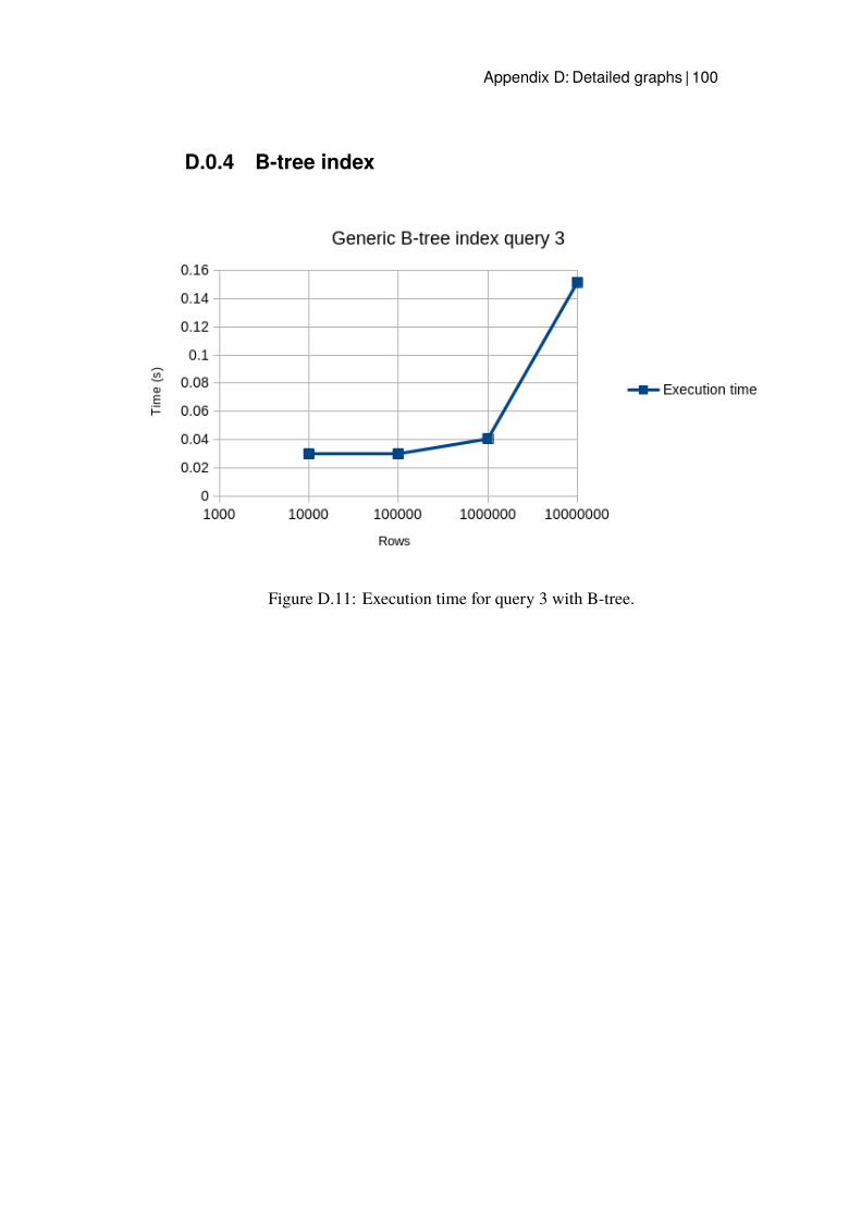
Appendix D: Detailed graphs | 100

D.0.4 B-tree index

Figure D.11: Execution time for query 3 with B-tree.

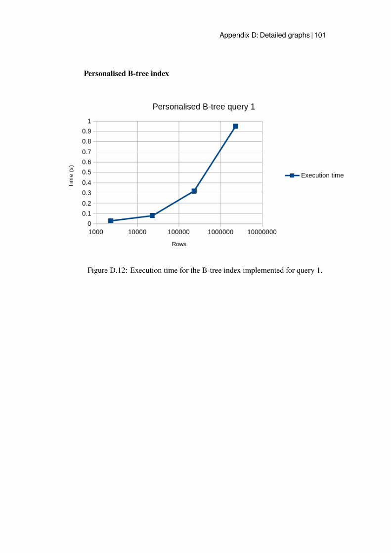
Appendix D: Detailed graphs | 101

Personalised B-tree index

Figure D.12: Execution time for the B-tree index implemented for query 1.

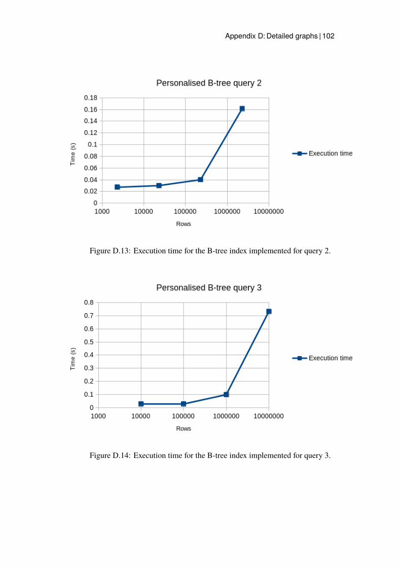
Appendix D: Detailed graphs | 102

Figure D.13: Execution time for the B-tree index implemented for query 2.

Figure D.14: Execution time for the B-tree index implemented for query 3.

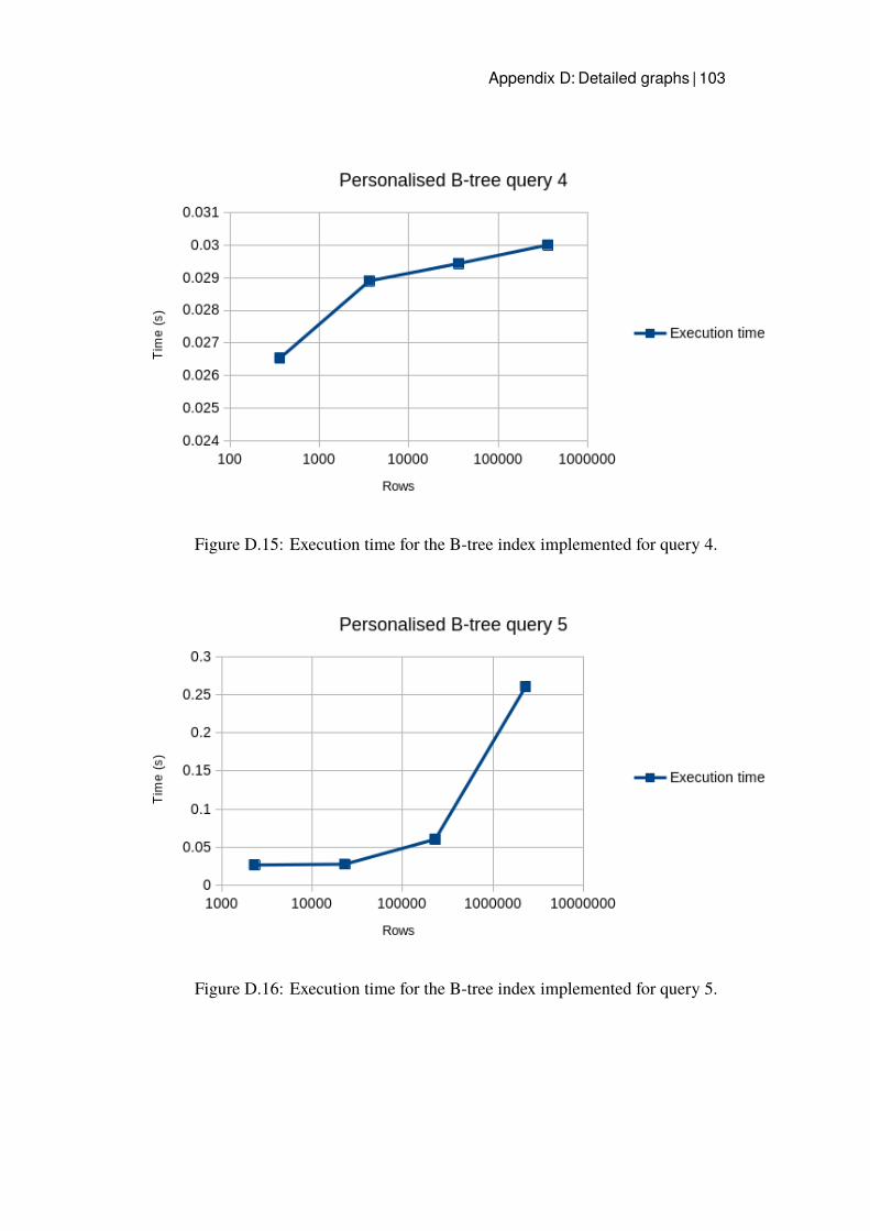
Appendix D: Detailed graphs | 103

Figure D.15: Execution time for the B-tree index implemented for query 4.

Figure D.16: Execution time for the B-tree index implemented for query 5.

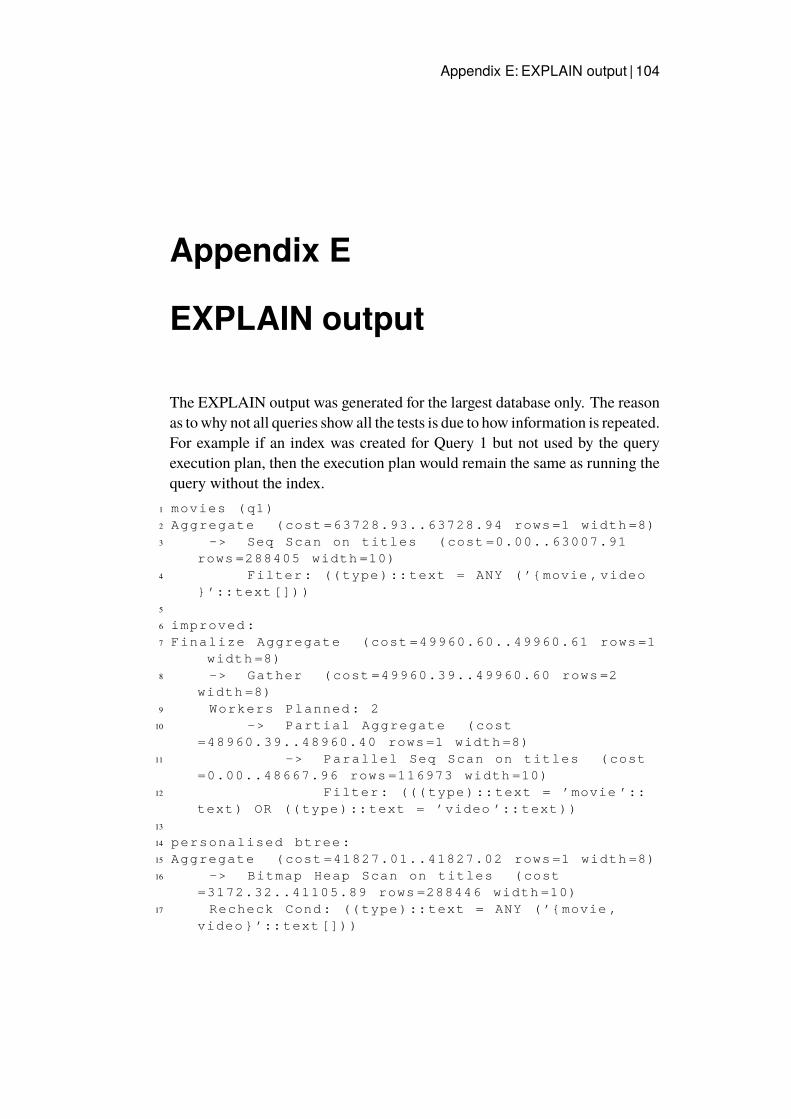
Appendix E: EXPLAIN output | 104

Appendix E

EXPLAIN output

The EXPLAIN output was generated for the largest database only. The reasonas towhy not all queries show all the tests is due to how information is repeated.For example if an index was created for Query 1 but not used by the queryexecution plan, then the execution plan would remain the same as running thequery without the index.

1 movies (q1)2 Aggregate ( cost =63728.93..63728.94 rows =1 width =8)3 -> Seq Scan on titles ( cost =0.00..63007.91

rows =288405 width =10)4 Filter : (( type ):: text = ANY ( ’{ movie , video

} ’:: text []) )5

6 improved :7 Finalize Aggregate ( cost =49960.60..49960.61 rows =1

width =8)8 -> Gather ( cost =49960.39..49960.60 rows =2

width =8)9 Workers Planned : 2

10 -> Partial Aggregate ( cost=48960.39..48960.40 rows =1 width =8)

11 -> Parallel Seq Scan on titles ( cost=0.00..48667.96 rows =116973 width =10)

12 Filter : ((( type ):: text = ’movie ’::text ) OR (( type ):: text = ’video ’:: text ))

13

14 personalised btree :15 Aggregate ( cost =41827.01..41827.02 rows =1 width =8)16 -> Bitmap Heap Scan on titles ( cost

=3172.32..41105.89 rows =288446 width =10)17 Recheck Cond : (( type ):: text = ANY ( ’{ movie ,

video } ’:: text []) )

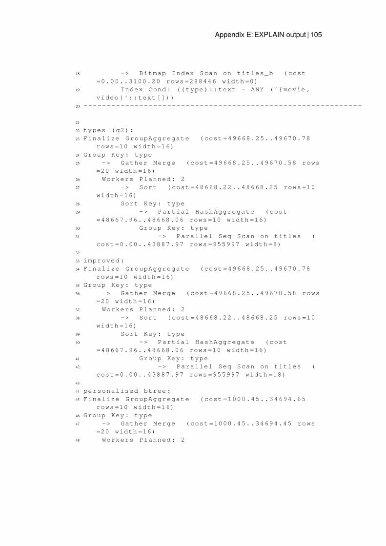
Appendix E: EXPLAIN output | 105

18 -> Bitmap Index Scan on titles_b ( cost=0.00..3100.20 rows =288446 width =0)

19 Index Cond : (( type ):: text = ANY ( ’{ movie ,video } ’:: text []) )

20 ------------------------------------------------------------

21

22 types (q2):23 Finalize GroupAggregate ( cost =49668.25..49670.78

rows =10 width =16)24 Group Key : type25 -> Gather Merge ( cost =49668.25..49670.58 rows

=20 width =16)26 Workers Planned : 227 -> Sort ( cost =48668.22..48668.25 rows =10

width =16)28 Sort Key : type29 -> Partial HashAggregate ( cost

=48667.96..48668.06 rows =10 width =16)30 Group Key : type31 -> Parallel Seq Scan on titles (

cost =0.00..43887.97 rows =955997 width =8)32

33 improved :34 Finalize GroupAggregate ( cost =49668.25..49670.78

rows =10 width =16)35 Group Key : type36 -> Gather Merge ( cost =49668.25..49670.58 rows

=20 width =16)37 Workers Planned : 238 -> Sort ( cost =48668.22..48668.25 rows =10

width =16)39 Sort Key : type40 -> Partial HashAggregate ( cost

=48667.96..48668.06 rows =10 width =16)41 Group Key : type42 -> Parallel Seq Scan on titles (

cost =0.00..43887.97 rows =955997 width =18)43

44 personalised btree :45 Finalize GroupAggregate ( cost =1000.45..34694.65

rows =10 width =16)46 Group Key : type47 -> Gather Merge ( cost =1000.45..34694.45 rows

=20 width =16)48 Workers Planned : 2

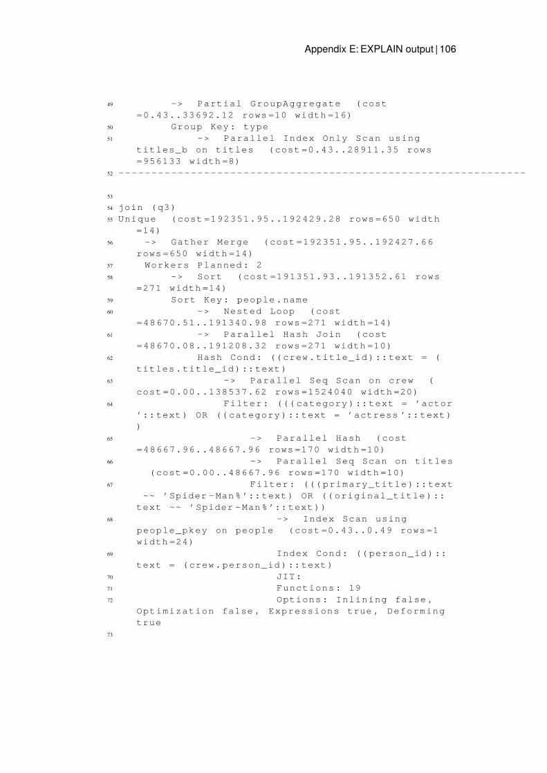
Appendix E: EXPLAIN output | 106

49 -> Partial GroupAggregate ( cost=0.43..33692.12 rows =10 width =16)

50 Group Key : type51 -> Parallel Index Only Scan using

titles_b on titles ( cost =0.43..28911.35 rows=956133 width =8)

52 --------------------------------------------------------------

53

54 join (q3)55 Unique ( cost =192351.95..192429.28 rows =650 width

=14)56 -> Gather Merge ( cost =192351.95..192427.66

rows =650 width =14)57 Workers Planned : 258 -> Sort ( cost =191351.93..191352.61 rows

=271 width =14)59 Sort Key : people . name60 -> Nested Loop ( cost

=48670.51..191340.98 rows =271 width =14)61 -> Parallel Hash Join ( cost

=48670.08..191208.32 rows =271 width =10)62 Hash Cond : (( crew . title_id ):: text = (

titles . title_id ):: text )63 -> Parallel Seq Scan on crew (

cost =0.00..138537.62 rows =1524040 width =20)64 Filter : ((( category ):: text = ’actor

’:: text ) OR (( category ):: text = ’actress ’:: text ))

65 -> Parallel Hash ( cost=48667.96..48667.96 rows =170 width =10)

66 -> Parallel Seq Scan on titles( cost =0.00..48667.96 rows =170 width =10)

67 Filter : ((( primary_title ):: text~~ ’Spider - Man % ’:: text ) OR (( original_title )::

text ~~ ’Spider - Man % ’:: text ))68 -> Index Scan using

people_pkey on people ( cost =0.43..0.49 rows =1width =24)

69 Index Cond : (( person_id )::text = ( crew . person_id ):: text )

70 JIT :71 Functions : 1972 Options : Inlining false ,

Optimization false , Expressions true , Deformingtrue

73

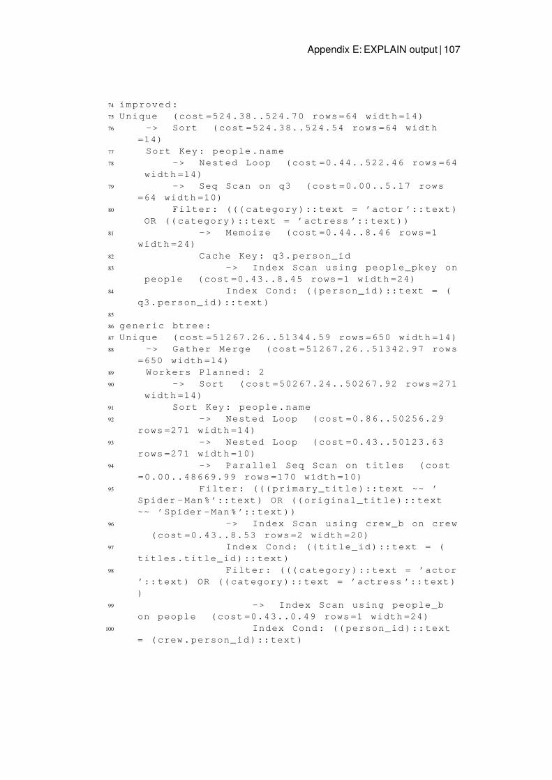
Appendix E: EXPLAIN output | 107

74 improved :75 Unique ( cost =524.38..524.70 rows =64 width =14)76 -> Sort ( cost =524.38..524.54 rows =64 width

=14)77 Sort Key : people . name78 -> Nested Loop ( cost =0.44..522.46 rows =64

width =14)79 -> Seq Scan on q3 ( cost =0.00..5.17 rows

=64 width =10)80 Filter : ((( category ):: text = ’actor ’:: text )

OR (( category ):: text = ’actress ’:: text ))81 -> Memoize ( cost =0.44..8.46 rows =1

width =24)82 Cache Key : q3. person_id83 -> Index Scan using people_pkey on

people ( cost =0.43..8.45 rows =1 width =24)84 Index Cond : (( person_id ):: text = (

q3. person_id ):: text )85

86 generic btree :87 Unique ( cost =51267.26..51344.59 rows =650 width =14)88 -> Gather Merge ( cost =51267.26..51342.97 rows

=650 width =14)89 Workers Planned : 290 -> Sort ( cost =50267.24..50267.92 rows =271

width =14)91 Sort Key : people . name92 -> Nested Loop ( cost =0.86..50256.29

rows =271 width =14)93 -> Nested Loop ( cost =0.43..50123.63

rows =271 width =10)94 -> Parallel Seq Scan on titles ( cost

=0.00..48669.99 rows =170 width =10)95 Filter : ((( primary_title ):: text ~~ ’

Spider - Man % ’:: text ) OR (( original_title ):: text~~ ’Spider - Man % ’:: text ))

96 -> Index Scan using crew_b on crew( cost =0.43..8.53 rows =2 width =20)

97 Index Cond : (( title_id ):: text = (titles . title_id ):: text )

98 Filter : ((( category ):: text = ’actor’:: text ) OR (( category ):: text = ’actress ’:: text ))

99 -> Index Scan using people_bon people ( cost =0.43..0.49 rows =1 width =24)

100 Index Cond : (( person_id ):: text= ( crew . person_id ):: text )

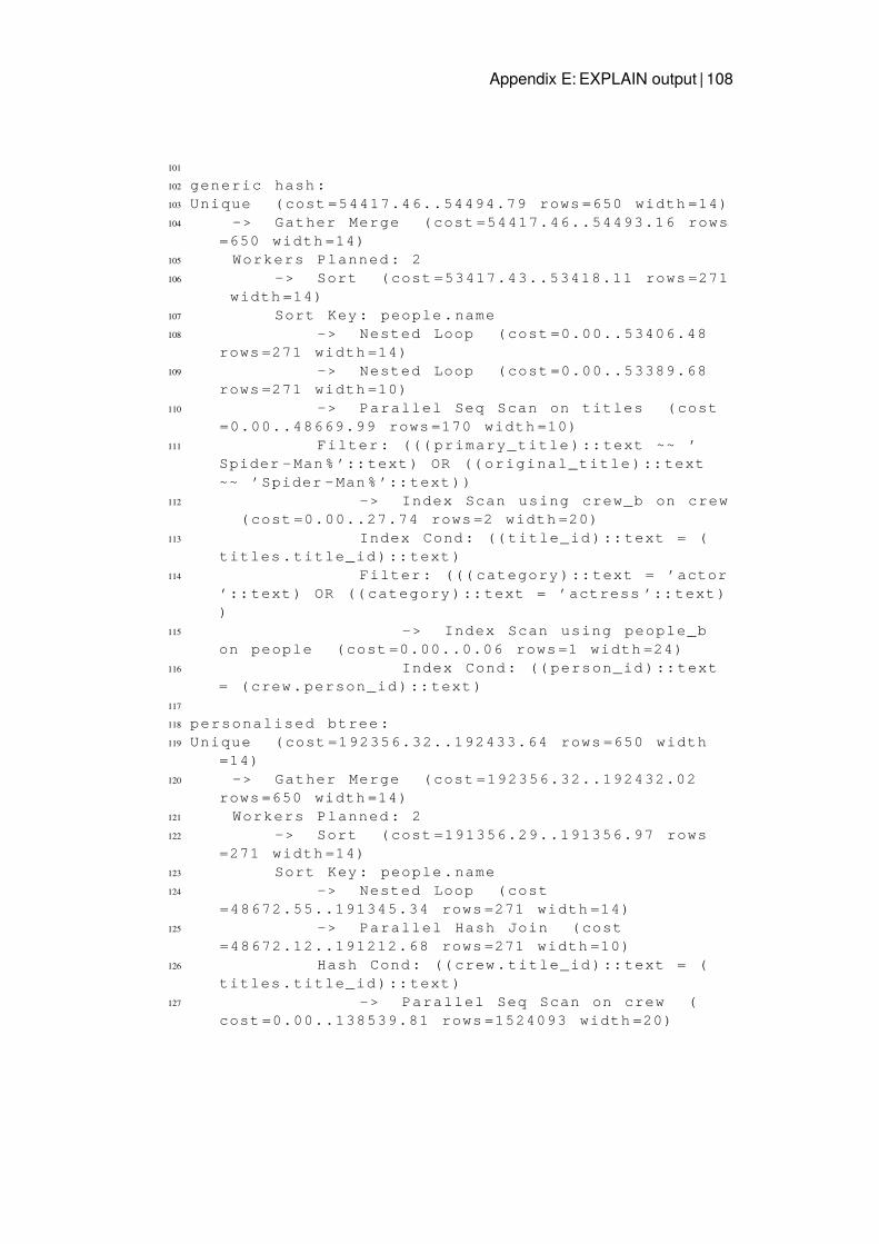
Appendix E: EXPLAIN output | 108

101

102 generic hash :103 Unique ( cost =54417.46..54494.79 rows =650 width =14)104 -> Gather Merge ( cost =54417.46..54493.16 rows

=650 width =14)105 Workers Planned : 2106 -> Sort ( cost =53417.43..53418.11 rows =271

width =14)107 Sort Key : people . name108 -> Nested Loop ( cost =0.00..53406.48

rows =271 width =14)109 -> Nested Loop ( cost =0.00..53389.68

rows =271 width =10)110 -> Parallel Seq Scan on titles ( cost

=0.00..48669.99 rows =170 width =10)111 Filter : ((( primary_title ):: text ~~ ’

Spider - Man % ’:: text ) OR (( original_title ):: text~~ ’Spider - Man % ’:: text ))

112 -> Index Scan using crew_b on crew( cost =0.00..27.74 rows =2 width =20)

113 Index Cond : (( title_id ):: text = (titles . title_id ):: text )

114 Filter : ((( category ):: text = ’actor’:: text ) OR (( category ):: text = ’actress ’:: text ))

115 -> Index Scan using people_bon people ( cost =0.00..0.06 rows =1 width =24)

116 Index Cond : (( person_id ):: text= ( crew . person_id ):: text )

117

118 personalised btree :119 Unique ( cost =192356.32..192433.64 rows =650 width

=14)120 -> Gather Merge ( cost =192356.32..192432.02

rows =650 width =14)121 Workers Planned : 2122 -> Sort ( cost =191356.29..191356.97 rows

=271 width =14)123 Sort Key : people . name124 -> Nested Loop ( cost

=48672.55..191345.34 rows =271 width =14)125 -> Parallel Hash Join ( cost

=48672.12..191212.68 rows =271 width =10)126 Hash Cond : (( crew . title_id ):: text = (

titles . title_id ):: text )127 -> Parallel Seq Scan on crew (

cost =0.00..138539.81 rows =1524093 width =20)

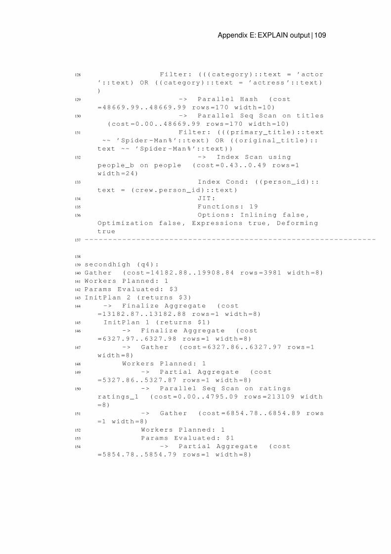
Appendix E: EXPLAIN output | 109

128 Filter : ((( category ):: text = ’actor’:: text ) OR (( category ):: text = ’actress ’:: text ))

129 -> Parallel Hash ( cost=48669.99..48669.99 rows =170 width =10)

130 -> Parallel Seq Scan on titles( cost =0.00..48669.99 rows =170 width =10)

131 Filter : ((( primary_title ):: text~~ ’Spider - Man % ’:: text ) OR (( original_title )::

text ~~ ’Spider - Man % ’:: text ))132 -> Index Scan using

people_b on people ( cost =0.43..0.49 rows =1width =24)

133 Index Cond : (( person_id )::text = ( crew . person_id ):: text )

134 JIT :135 Functions : 19136 Options : Inlining false ,

Optimization false , Expressions true , Deformingtrue

137 --------------------------------------------------------------

138

139 secondhigh (q4):140 Gather ( cost =14182.88..19908.84 rows =3981 width =8)141 Workers Planned : 1142 Params Evaluated : $3143 InitPlan 2 ( returns $3)144 -> Finalize Aggregate ( cost

=13182.87..13182.88 rows =1 width =8)145 InitPlan 1 ( returns $1)146 -> Finalize Aggregate ( cost

=6327.97..6327.98 rows =1 width =8)147 -> Gather ( cost =6327.86..6327.97 rows =1

width =8)148 Workers Planned : 1149 -> Partial Aggregate ( cost

=5327.86..5327.87 rows =1 width =8)150 -> Parallel Seq Scan on ratings

ratings_1 ( cost =0.00..4795.09 rows =213109 width=8)

151 -> Gather ( cost =6854.78..6854.89 rows=1 width =8)

152 Workers Planned : 1153 Params Evaluated : $1154 -> Partial Aggregate ( cost

=5854.78..5854.79 rows =1 width =8)

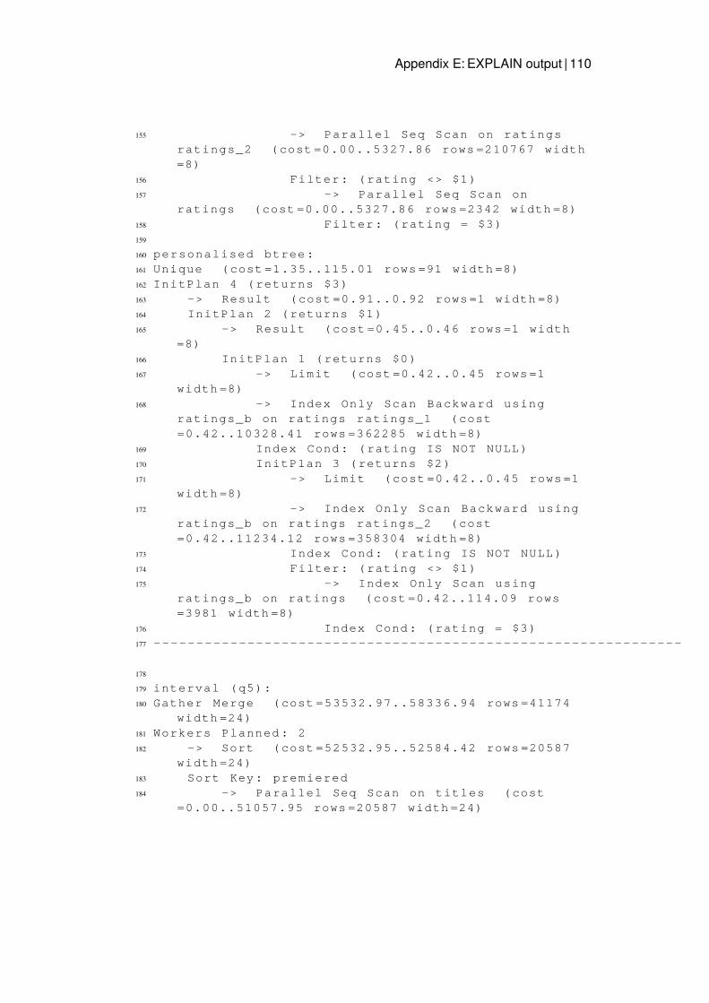
Appendix E: EXPLAIN output | 110

155 -> Parallel Seq Scan on ratingsratings_2 ( cost =0.00..5327.86 rows =210767 width=8)

156 Filter : ( rating <> $1)157 -> Parallel Seq Scan on

ratings ( cost =0.00..5327.86 rows =2342 width =8)158 Filter : ( rating = $3)159

160 personalised btree :161 Unique ( cost =1.35..115.01 rows =91 width =8)162 InitPlan 4 ( returns $3)163 -> Result ( cost =0.91..0.92 rows =1 width =8)164 InitPlan 2 ( returns $1)165 -> Result ( cost =0.45..0.46 rows =1 width

=8)166 InitPlan 1 ( returns $0)167 -> Limit ( cost =0.42..0.45 rows =1

width =8)168 -> Index Only Scan Backward using

ratings_b on ratings ratings_1 ( cost=0.42..10328.41 rows =362285 width =8)

169 Index Cond : ( rating IS NOT NULL )170 InitPlan 3 ( returns $2)171 -> Limit ( cost =0.42..0.45 rows =1

width =8)172 -> Index Only Scan Backward using

ratings_b on ratings ratings_2 ( cost=0.42..11234.12 rows =358304 width =8)

173 Index Cond : ( rating IS NOT NULL )174 Filter : ( rating <> $1)175 -> Index Only Scan using

ratings_b on ratings ( cost =0.42..114.09 rows=3981 width =8)

176 Index Cond : ( rating = $3)177 --------------------------------------------------------------

178

179 interval (q5):180 Gather Merge ( cost =53532.97..58336.94 rows =41174

width =24)181 Workers Planned : 2182 -> Sort ( cost =52532.95..52584.42 rows =20587

width =24)183 Sort Key : premiered184 -> Parallel Seq Scan on titles ( cost

=0.00..51057.95 rows =20587 width =24)

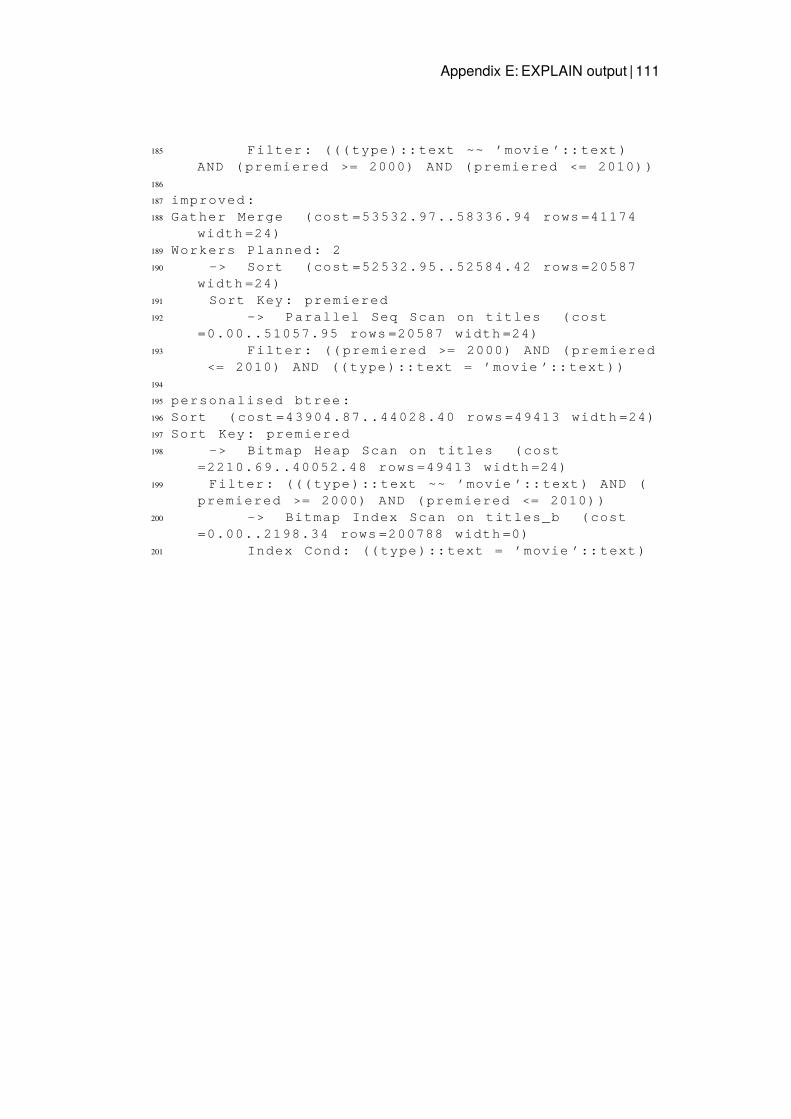
Appendix E: EXPLAIN output | 111

185 Filter : ((( type ):: text ~~ ’movie ’:: text )AND ( premiered >= 2000) AND ( premiered <= 2010) )

186

187 improved :188 Gather Merge ( cost =53532.97..58336.94 rows =41174

width =24)189 Workers Planned : 2190 -> Sort ( cost =52532.95..52584.42 rows =20587

width =24)191 Sort Key : premiered192 -> Parallel Seq Scan on titles ( cost

=0.00..51057.95 rows =20587 width =24)193 Filter : (( premiered >= 2000) AND ( premiered

<= 2010) AND (( type ):: text = ’movie ’:: text ))194

195 personalised btree :196 Sort ( cost =43904.87..44028.40 rows =49413 width =24)197 Sort Key : premiered198 -> Bitmap Heap Scan on titles ( cost

=2210.69..40052.48 rows =49413 width =24)199 Filter : ((( type ):: text ~~ ’movie ’:: text ) AND (

premiered >= 2000) AND ( premiered <= 2010) )200 -> Bitmap Index Scan on titles_b ( cost

=0.00..2198.34 rows =200788 width =0)201 Index Cond : (( type ):: text = ’movie ’:: text )

Appendix F: Database link | 112

Appendix F

Database link

https://canvas.kth.se/courses/19966/files/3413108/download

TRITA-EECS-EX-2021:821

www.kth.se