Comparing Classes of Finite Structures

arX

iv:0

803.

3291

v1 [

mat

h.L

O]

22

Mar

200

8

Comparing classes of finite structures

W. Calvert, D. Cummins, J. F. Knight, and S. Miller

December 7, 2013

1 Introduction

In many branches of mathematics, there is work classifying a collection of ob-jects, up to isomorphism or other important equivalence, in terms of nice in-variants. In descriptive set theory, there is a body of work using a notion of“Borel embedding” to compare the classification problems for various classes ofstructures (fields, graphs, groups, etc.) [7], [3], [11], [12], [13]. In this work, eachclass consists of structures with the same countable universe, say ω, and withthe same language, usually finite. For a given finite language L, the class of allL-structures with universe ω has a natural topological structure, and the otherclasses of L-structures being considered are normally Borel subclasses of these.

A Borel embedding of one class K into another class K ′ is a Borel functionfrom K to K ′ that is well defined and 1−1 on isomorphism types. The notationK ≤B K ′ indicates that there is such an embedding. If K ≤B K ′, then the clas-sification problem for K reduces to that for K ′. If K ′ has nice invariants, thenwe may describe A ∈ K, up to isomorphism, by determining the correspondingB ∈ K ′ and giving its invariants. If there is no nice classification for K, thenthe same must be true for K ′.

Example: Friedman and Stanley [7] described an embedding of the class ofundirected graphs in the class of fields of characteristic 0. The edge relation onan undirected graph is assumed to be irreflexive. For an undirected graph G,the corresponding field is obtained by first taking an algebraically closed field ofcharacteristic 0, with a transcendence base G, identified with the set of graphelements, and then restricting to the subfield that is generated by the algebraicclosures of the single elements b ∈ G, and the elements

√b1 + b2, where b1, b2

are joined by an edge in G.

In the present paper, our goal is to compare classes of structures using anotion of computable embedding. Like the relation ≤B, our relation ≤c is apartial order on classes of structures. We focus mainly, but not exclusively,on classes of finite structures. We have some “landmark” classes—finite primefields, finite linear orders, finite dimensional vector spaces over the rationals, andarbitrary linear orders—forming a strictly increasing sequence. If we restrict ourattention to classes of finite structures, then the class of finite linear orders lies on

1

top, along with the class of finite cyclic groups and the class of finite undirectedgraphs. There are many incomparable classes below the class of finite primefields, and between that and the class of finite linear orders. If we allow classesthat contain infinite structures, then the class of undirected graphs lies on top.The Friedman-Stanley embedding can be turned into a computable embedding,showing that the class of fields of characteristic 0 is also on top. There aremany incomparable classes between the class of finite linear orders and the classof finite dimensional vector spaces, and between this class and the class of alllinear orders.

In the remainder of the present section, we give some conventions and defi-nitions. In Section 2, we discuss various natural examples of classes. We showthat any class of finite structures can be computably embedded in the class offinite undirected graphs, and this can be computably embedded in the class offinite linear orders. In Section 3, we characterize the classes that can be com-putably embedded in the finite prime fields, and those that can be computablyembedded in the finite linear orders. In Section 4, we show that the class offinite dimensional vector spaces over the rationals lies strictly above the classof finite linear orders. Using notions related to immunity, we construct fami-lies of 2ℵ0 incomparable classes in various intervals. We also produce infiniteincreasing chains of classes. Finally, in Section 5, we state some open problems.

1.1 Conventions

We begin with some conventions. The structures that we consider all have afinite relational language, and all have universe a subset of ω. The classes thatwe consider all consist of structures for a single language. Moreover, all classesare closed under isomorphism, modulo the restriction that each structure hasuniverse a subset of ω. We will sometimes identify a structure A with its atomicdiagram D(A). We will also identify finite sequences, sentences, etc., with theirGodel numbers. Thus, we may say that a structure is computable, meaning thatthe set of codes for sentences in D(A) is computable. All finite structures arecomputable, but the infinite structures that we consider may or may not becomputable.

1.2 Basic definitions

There are several possible notions of computable transformation from one classof structures to another. The one that we have chosen is essentially uniformenumeration reducibility. Recall that for A, B ⊆ ω, B is enumeration reducibleto A if there is a computably enumerable (c.e.) set Φ of pairs (α, b), where α isa finite subset of ω and b ∈ ω, such that

B = {b|(∃α ⊆ A) (α, b) ∈ Φ} .

For a given Φ and A, the set B is unique, and we may denote it by Φ(A). (Formore on enumeration reducibility, see Rogers [19].)

Here is the definition of computable transformation that we shall use.

2

Definition 1. Let K and K ′ be classes of structures, and let Φ be a c.e. set ofpairs (α, ϕ), where α is a subset of the atomic diagram of a finite structure forthe language of K, and ϕ is an atomic sentence, or the negation of one, in thelanguage of K ′. We say that Φ is a computable transformation from K to K ′

if for all A ∈ K, Φ(D(A)) has the form D(B), for some B ∈ K ′. We may writeΦ(A) = B (identifying the structures with their atomic diagrams).

Note that in this definition, the output D(B) depends only on the inputD(A), not on the order in which it is examined.

Proposition 1.1. Let K, K ′ be classes of structures, and let Φ be a computabletransformation from K to K ′. If A,A′ ∈ K, where A ⊆ A′, then Φ(A) ⊆ Φ(A′).

Proof. Let B = Φ(A), and let B′ = Φ(A′). If ϕ ∈ D(B), then there is a finite setα ⊆ D(A) such that (α, ϕ) ∈ Φ. Then since α ⊆ D(A′), we have ϕ ∈ D(B′).

It follows from Proposition 1.1 that if K contains an infinite strictly increas-ing chain of structures (increasing under the substructure relation), then so doesK ′. More generally, we have the following.

Corollary 1.2. Let K, K ′ be classes of structures such that there is a com-putable transformation from K to K ′. If K contains a strictly increasing chainof structures having order type ρ, then so does K ′.

We are interested in computable transformations that respect isomorphism,mapping K/∼= into K ′/∼= in a 1 − 1 way.

Definition 2. Let K, K ′ be classes of structures.

1. A computable embedding of K in K ′ is a computable transformation Φfrom K to K ′ such that for all A,A′ ∈ K, A ∼= A′ iff Φ(A) ∼= Φ(A′).

2. If there is a computable embedding of K in K ′, then we write K ≤c K ′.

The following proposition records two obvious, but useful, facts.

Proposition 1.3. Let K1, K2, K′1, K

′2 be classes of structures, with K ′

1 ⊆ K1

and K ′2 ⊇ K2. If K1 ≤c K2, via Φ, then K ′

1 ≤c K ′2, via the same Φ.

To illustrate what a computable embedding actually looks like, we return tothe motivating example.

Proposition 1.4 (Friedman and Stanley). If K is the class of undirectedgraphs, and K ′ is the class of fields of characteristic 0, then K ≤c K ′.

Sketch of proof. We describe the computable embedding Φ. First, let F bea computable algebraically closed field of characteristic 0, with a computablesequence (bk)k∈ω of elements that are algebraically independent. For an undi-rected graph G (with universe a subset of ω), let F(G) be the subfield of Fgenerated by the elements that are either in the algebraic closure of bk, for somegraph element k, or else have the form

√

bi + bj , where i, j are distinct graph

3

elements joined by an edge. Now, let Φ consist of the pairs (α, ϕ), where α isthe atomic diagram of some finite undirected graph G and ϕ is a sentence inthe atomic diagram of F(G). Clearly, Φ is c.e. For any A ∈ K, Φ(A) = F(A).Therefore, Φ is a computable transformation from K to K ′. The fact that Φ is1−1 on isomorphism types takes some effort. (It must be shown that for i, j ∈ G,if i, j are not joined by an edge, then

√

bi + bj is not present in F(G).)

Notation: We write C for the set of all classes of structures satisfying ourconventions, and FC for the restriction to classes of finite structures. Therelation ≤c is a partial order on C, and as always, we get an equivalence relation≡c, where K ≡c K ′ iff both K ≤c K ′ and K ′ ≤c K. The equivalence classesunder ≡c are called c-degrees. The relation ≤c on C induces a partial orderon c-degrees, which we denote also by ≤c. We write C for the degree structure(C/≡c

,≤c), and we write FC for the restriction of C to the c-degrees that containelements of FC.

1.3 Alternative definitions

Effective transformations between classes of structures, of one kind or another,occur in many places in the literature. We mention only a sample. First, thereare notions that involve interpretation, in which the universe and basic rela-tions of a structure A ∈ K are defined, in a uniform way, in the correspondingstructure B ∈ K ′. This approach has been used to show that certain theoriesare undecidable—see, for example, the unpublished typescript of Rabin andScott [18], or the more recent paper of Nies [17]. Sometimes, it is necessaryto have the interpretation go both ways. This happens, for example, in thepaper of Hirschfeldt, Khoussainov, Shore, and Slinko [10], with results on “com-putable dimension” (the number of isomorphic members not isomorphic by acomputable function) and “degree spectra” (the set of possible degrees of a re-lation in isomorphic copies of a computable structure). Some of our computableembeddings involve interpretions, but others do not.

Another kind of effective transformation, which is used in connection withcomputable structures, is a partial computable function taking indices for com-putable members of one class K to indices for computable members of anotherclass K ′. This approach occurs, for example, in the usual proof that the set ofcomputable indices for computable well orderings is Π1

1 complete (see Rogers[19]). More recently, the approach is used in [4], [5], in results on the complexityof the isomorphism relation. We deal directly with structures, not with indices,and the infinite structures that we consider are not necessarily computable.

We state two alternative notions of computable transformation that we triedworking with, and then discarded in favor of the one in Definition 1. In thedefinition below, enumeration reducibility is replaced by Turing reducibility.

Definition 1′: Let K, K ′ be classes of structures. Then Φ = ϕe (the computableoperator given by oracle machine e) is a computable transformation of K into

4

K ′ if for all A ∈ K, ϕD(A)e is the characteristic function of D(B), for some

B ∈ K ′.

Definition 1′ would be equivalent to Definition 1 if our structures all haduniverse ω. However, for most structures, there will be numbers not in theuniverse. Definition 1′ would have us use information about these numbers,which strikes us as not “structural”.

The other alternative definition has the feature that for a given input struc-ture A, the output structure B depends not just on D(A), but on the order inwhich we look at the information.

Definition 1′′: Let K, K ′ be classes of structures. An effective transformationof K into K ′ is a partial computable function f such that for all A ∈ K, andall chains (αs)s∈ω of finite sets such that D(A) = ∪sαs, there is a structureB ∈ K ′ such that D(B) is the union of a corresponding chain (βs)s∈ω of finitesets, where β0 = ∅, and for all s, βs+1 = f(βs, αs).

From Definition 1′, and also from Definition 1′′, we obtain obvious alternativeversions of Definition 2, and we get further partial orders on C and FC. UsingDefinition 1′′, we would produce transformations that respect isomorphism byguessing at the “global” structure. Definition 1′′ may be interesting from thepoint of view of computability theory, especially for classes of infinite structures.There is a great deal of guessing at global structure in known arguments showingthat the set of indices of computable copies of various structures is Σ1

1 completeor Π0

α-complete (see [4], [5]). We chose Definition 1 as representing a moredirect computable transformation of one structure into another, based on “local”structure. Proposition 1.1 seems intuitively right to us, and it fails for thealternative definitions.

1.4 Related reducibilities

There is quite a lot of work on the Medvedev lattice and Medvedev degrees(see [16], [22], [20]). The setting resembles ours in some ways. In both cases,the basic objects are classes, and the reducibility takes members of one classto members of another in a uniform effective way. Our reducibility relation isuniform enumeration reducibility, while Medvedev reducibility is uniform Tur-ing reducibility. Dyment developed a variant of the Medvedev lattice based onenumeration reducibility (see [22],[6]). In the Medvedev lattice, the points areclasses of functions, while we consider classes of structures, closed under isomor-phism. Moreover, our computable reductions are supposed to be well definedand 1 − 1 on isomorphism types. This makes our setting quite different. It willbe shown in [14] that C is not a lattice.

5

2 Examples

Having defined the notion of a computable embedding from one class of struc-tures into another, we will now investigate some natural examples of classes ofstructures. If we restrict our attention to classes of finite structures, we findthat there are two distinct c-degrees into which almost all natural examplesof classes of finite structures fall. One of these c-degrees is made up of thoseclasses that are computably equivalent to the prime fields, while the other con-tains classes of structures that are computably equivalent to finite linear orders(we will call these classes PF and FLO, respectively). We prove that these arein fact different c-degrees:

Proposition 2.1. PF �c FLO (i.e., PF ≤c FLO and FLO 6≤c PF ).

Proof. To show PF ≤c FLO, we construct a computable embedding Φ. Foreach n, let Ln, be the the usual linear order on the first n elements of the naturalnumbers. Let Φ be the set of pairs (α, ϕ) such that, for some n, α is the atomicdiagram of a field of size pn (where pn is the nth prime), and ϕ ∈ D(Ln). Thisset of pairs is clearly c.e. Note that, for all A,A′ ∈ PF , we have A ∼= A′ iffΦ(A) ∼= Φ(A′). Therefore, PF is computably embedded in PF .

To show that FLO �c PF , assume for a contradiction that FLO ≤c PF .Say Φ is a computable embedding. Let A,A′ be two nonisomorphic membersof FLO. Suppose A has fewer elements than A′. Then A is clearly isomorphicto a substructure of A′. We may suppose that A ⊆ A′. By Proposition 1.1,Φ(A) ⊆ Φ(A′). We also know from Definition 2 that Φ(A) ≇ Φ(A′). Since noprime field is a substructure of another, nonisomorphic prime field, we concludethat FLO �c PF .

We note that in the proof of Proposition 2.1 above, showing FLO �c PFonly used the fact that FLO contains two nonisomorphic finite linear orders.The same proof yields the following.

Corollary 2.2. If K is a class containing two nonisomorphic finite linear or-ders, then K 6≤c PF .

We have seen that there are at least two distinct c-degrees in FC. Mostnatural examples of classes of finite structures fit into one of these two c-degrees,but before we discuss some of these examples, it will be convienent to prove that,for classes of finite structures, the c-degree of FLO is the maximum element ofFC. We first prove the following lemma.

Lemma 2.3. For any class of structures K in a finite relational language,K ≤c UG, where UG is the class of undirected graphs. Moreover, if K consistsof finite structures, then K ≤c FUG, where FUG is the class of finite undirectedgraphs.

Proof. For each finite relational language L, we describe a computable embed-ding Φ of the class of all L-structures into UG. Thus, for an arbitrary class ofL-structures whose universes are subsets of the natural numbers, Φ embeds the

6

✉ ✉

✉g(1)

✡✡✡❏

❏❏ ✉ ✉

✉g(2)

✡✡✡❏

❏❏ ✉ ✉

✉g(3)

✡✡✡❏

❏❏

Figure 1: Representing the elements 1, 2, 3

✉

✉

✉✉

✉

g✚

✚✚

❚❚❚☞

☞☞

❩❩❩

✧✧

✧✧

✧✧

✧✧✧❜

❜❜

❜❜

❜❜

❜❜

✉ ✉

✉g(1)

✡✡✡❏

❏❏

✉

✉

✉

✉ ✉

✉g(2)

✡✡✡❏

❏❏ ✉ ✉

✉g(3)

✡✡✡❏

❏❏

Figure 2: Representing R(1, 2, 3), where R corresponds to 5

given class in UG. The embedding Φ will have the feature that if A is a finiteL-structure, then Φ(A) is also finite.

We begin by describing a large undirected graph G, with finite subgraphsthat represent possible elements of L-structures, and further finite subgraphsthat represent sentences R(a1, . . . , ar) which may occur in the atomic diagramsof L-structures. The graph G will be computable.

Subgraphs representing possible elements

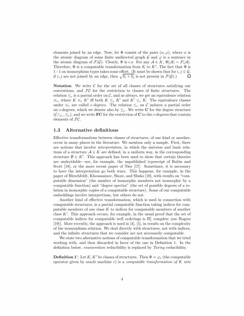
For each a ∈ ω, we put into G a 3-cycle Ta. We arrange that the cycles Ta

are all disjoint, and we can pass effectively from a to Ta. Let g(a) be the leastelement of Ta. (Figure 1 shows T1, T2, and T3.)

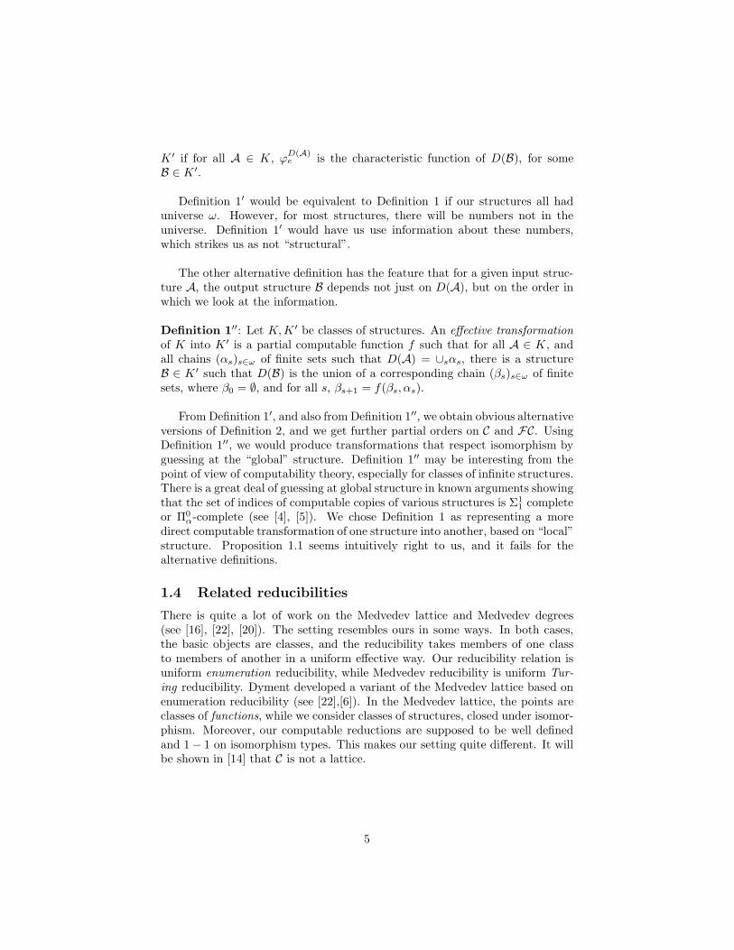
Subgraphs representing possible atomic sentences

We assign to the relation symbols of L distinct numbers greater than 3.Suppose R is assigned the number k. Then for each atomic sentence of the formρ = R(a1, . . . , ar), we put into G a subgraph Gρ consisting of a k-cycle togetherwith some connecting chains. Say g is the least element of the k-cycle. Weconnect g to g(a1) by a chain of length 1, adding just an edge. We connect gto g(a2) by a chain of length 2, adding an intermediate point, and, in general,we connect g to ai by a chain of length i, adding i − 1 intermediate points.All of the points that we have described as making up the subgraph Gρ are

7

distinct, and for distinct ρ, the subgraphs Gρ are disjoint, except possibly forthe elements g(a) (in the 3-cycles. We arrange the construction so that we canpass effectively from an atomic sentence ρ to the subgraph Gρ. (Figure 2 givesa sample Gρ.)

The graph G is generated by the two families of subgraphs described above.For each L-structure A, there is a corresponding graph G(A) ⊆ G, generated bythe subgraphs Ta, where a ∈ A, and Gρ, where ρ is a sentence in D(A) of theform R(a1, . . . , an). We note that if A is finite, then G(A) is also finite. Now,we are ready to define the computable embedding Φ. This consists of the pairs(α, ϕ) such that for some finite L-structure A, α = D(A) and ϕ ∈ D(G(A)).

The set Φ is c.e. For any L-structure A, Φ(A) = G(A). It should be clearthat if A ∼= A′,then Φ(A) ∼= Φ(A′). Conversely, ifΦ(A) ∼= Φ(A′), then the 3-cycles in Φ(A) must correspond to the 3-cycles in Φ(A′). So, the isomorphismfrom Φ(A) onto Φ(A′) induces a 1−1 function from A onto A′. Moreover, if forsome atomic sentence ρ = R(a1, . . . , ar), the 3-cycles in Φ(A) corresponding toa1, . . . , ar are attached to the subgraph Gρ, indicating that A |= R(a1, . . . , ar),then the corresponding 3-cycles in Φ(A′) are attached to a copy of Gρ, indicatingthat A′ |= R(f(a1), . . . , f(ar)). It follows that A ∼= A′. Therefore, Φ is acomputable embedding of the class of all L-structures into UG.

Definition 3.

1. A computable enumeration of a class K is a c.e. set E of pairs (n, ϕ)where n ∈ ω and ϕ is an atomic sentence or the negation of one, and

(a) for each n, {ϕ|(n, ϕ) ∈ E} = D(An), for some An ∈ K,

(b) for each A ∈ K, there is some n such that An∼= A.

We may write (An)n∈ω instead of E for the enumeration, indicating thatit really is a list.

2. An enumeration (An)n∈ω of a class K is Friedberg if each isomorphismtype in K is represented just once on the list.

The following lemma says that FUG has a computable Friedberg enumera-tion of a special kind.

Lemma 2.4. There is a computable Friedberg enumeration (Gn)n∈ω of FUGwith the feature that if G ∼= Gm and G′ ∼= Gn, where G′ is a proper extension ofG, then m < n.

Proof. To prove the lemma, we first define a partial order on the class of finiteundirected graphs as follows. One graph is greater than another if it has morevertices than the other. If two graphs have the same number of vertices, but onehas more edges than the other, the one with more edges is greater. Two graphs

8

are said to be equivalent if they agree in number of vertices and in number ofedges—equivalent graphs need not be isomorphic. Since, for a given set numberof vertices and set number of edges, there will only be a finite number of differentways to arrange the edges, it is obvious that any equivalence class on this partialorder will only have a finite number of members. Also, since the number of edgesa graph may contain is bounded by the number of pairs of vertices the graphcontains, for graphs of a given number of vertices, there will only be a finitenumber of equivalence classes.

To build the Friedberg enumeration, we run through the equivalence classes,in increasing order, and within a given equivalence class, we choose a singlerepresentative of each isomorphism type to put into our list. Since, for eachequivalence class, we have only a finite number of possible edge arrangements,we can do this effectively. Since every finite undirected graph falls into one ofthe equivalence classes, our enumeration will include every isomprphism typeof finite undirected graphs. It is a Friedberg enumeration since if two membersof FUG are isomorphic, they will be in the same equivalence class, and foreach equivalence class we included just one representative of each isomorphismtype.

Using Lemma 2.4, we can prove the following.

Theorem 2.5. FUG ≡c FLO

Proof. We must define a computable embedding Φ of FUG into FLO. Take thecomputable Friedberg enumeration (Gn)n∈ω of FUG with the special feature inLemma 2.4. For each n, let Ln be the usual linear ordering of {0, 1, 2...n− 1}.Let Φ be the set of pairs (α, ϕ) such that for some n, α is the atomic diagram ofa copy of Gn and ϕ ∈ D(Ln). This set of pairs is clearly c.e. For each G ∈ FUG,there is a unique n such that G ∼= Gn. Then we have Φ(G) = Ln—here we areusing the special feature of our Friedberg enumeration, which guarantees thatif G′ ⊆ G, where G′ ∼= Gm, then m ≤ n. It follows that Φ is well defined and1 − 1 on isomorphism types. We have shown that FUG ≤c FLO. We get thefact that FLO ≤c FUG directly from Lemma 2.3 and Proposition 1.3.

Having shown that the c-degree of FLO is at the top of the FC, we go on toshow that there are further c-degrees (containing classes of infinite structures)that lie above that of FLO.

Theorem 2.6. The class FV S of finite dimensional vector spaces over therationals lies strictly above FLO; that is, FLO � FV S.

Proof. Before proving the result, we should specify the language we are usingfor vector spaces. It is L = {V, F, 0F , 1F , +F , ∗F , 0V , +V , ∗V}, where 0F , 1F ,+F , ∗F are zero, one, addition and mulitplication in the rationals, and 0V , +V ,and ∗V are the zero vector, vector addition, and multiplication of a scalar bya vector, respectively. Inlcuding the field symbols in our language allows us toavoid including a separate symbol for multiplication by each scalar (a common

9

approach). Thus, our language is finite. We make it relational by thinking ofthe binary operations and constants as relations.

To prove that FLO ≤c FDS, let V be a computable vector space over therationals, with a computable sequence of basis elements b1, b2, . . .. For each n,let Vn be the subspace of V with basis {b1, . . . , bn}. Let Φ be the set of pairs,(α, ϕ) such that for some n, α is the atomic diagram of a linear ordering of sizen and ϕ ∈ D(Vn). The set Φ is clearly c.e. Note that, for all A,A′ ∈ FLO,A ∼= A′ iff Φ(A) ∼= Φ(A′). Only the number of elements in A was consideredin the construction of Φ, so Φ will map every member of a given isomorphismtype of FLO to the same member of FDS.

To prove that FDS �c FLO, we first observe that for any finite set of atomicsentences α in the language of rational vector spaces, plus natural numbers, α isa subset of the atomic diagram of a vector space of any given finite dimension.If α describes n independent vectors in a vector space V , it is obvious that αis a subset of atomic diagrams of vector spaces of dimension greater than n,but it is also true that α is a subset of the atomic diagrams of vector spaces ofdimension less than n. This is because, since α is finite, the sentences it containscan only describe a finite number of linear combinations of the n vectors, sayingthat these are not 0. We may extend α to β, with a sentence saying that somefurther linear combination of two of the vectors is 0, so that β is a subset of thediagram of a vector space V ′ of dimension n − 1.

To show that FDS �c FLO, assume towards a contradiction that thereexists a Φ witnessing FDS ≤c FLO. Let V be a two-dimensional member ofFDS, and say that Φ(V) = L, where L is an ordering of type n. There is a finiteset of pairs (α1, ϕ1), . . . , (αr, ϕr) in Φ such that D(L) = {ϕ1, . . . , ϕr}. Thenα = ∪1≤i≤rαi is a finite subset of D(V). We saw above that the set α is alsoa subset of the atomic diagram of a rational vector space V ′ of dimension one.Since α ⊆ D(V ′), Φ(V ′) must be a linear order, say L′, such that D(L) ⊆ D(L′).Therefore, either L′ ∼= L, or L ⊂ L′. If L′ ∼= L, then Φ is not one to one onisomorphism types. If L ⊂ L′, then Proposition 1.1 would fail for Φ. Eitherway, we have our contradiction.

Note that in the proof that FDS 6≤c FLO, where we used dimensions oneand two, we could have substituted any two different dimensions.

Corollary 2.7. If K is a class containing vector spaces of two different dimen-sions, then K 6≤c FLO.

3 General Characteristics

The natural examples of classes described in Section 2 give rise to broaderquestions regarding our ability to determine what key characteristics of thoseclasses are essential for their placement in our structure. Our goal was to givegeneral results that determine where an arbitrary class lies in relation to thelandmark examples, and then manipulate those results in order to constructmore examples to fill in our partial order. For simplicity, we now will refer to

10

the c-degree containing finite prime fields as Type I and the c-degree containingfinite linear orders and finite undirected graphs as Type II. Most generally, weknow that all classes of finite structures will embed into a class of Type II, fromLemma 2.3. We would like to know what is required for an arbitrary class (ofpossibly infinite structures) to embed in a class of Type II. We would also liketo know which classes lie above and below those of Type I.

3.1 Results relating to Type I

Our examples in Section 2 suggested the abstract conditions on a class of struc-tures K that are required for Type I ≤c K. The conditions involve computableFriedberg enumerations (defined in Section 2). It is well-known that there areclasses with a computable enumeration but no computable Friedberg enumera-tion, although we have not been able to determine who first showed this. Thereare familiar examples, such as the class of computable linear orderings. Below,we construct a simple example, consisting of finite structures.

Proposition 3.1. There is a class of finite structures K that has a computableenumeration but no computable Friedberg enumeration.

Proof. We want to create a class K with a computable enumeration E . Foreach n, the set {ϕ|(n, ϕ) ∈ E} should be the diagram of some An ∈ K, and eachelement of K should be isomorphic to An, for some n. For each e, we have arequirement Re stating that We is not a computable Friedberg enumeration ofK; either We fails to be an enumeration of K, or else it repeats isomorphismtypes.

At each stage s, we have enumerated a finite subset of E , attempting to takecare of the first s requirements. Our strategy for Re is as follows: Let C be ane-cycle, and let C− be the result of adding to C an extra “tail”—that is, an extravertex connected to exactly one vertex of the cycle. We initiate the requirementby putting into E pairs (2e, ϕ) for all ϕ ∈ D(C) and (2e+1, ϕ) for all ϕ ∈ D(C−).Suppose at some later stage t, we see, for some B ∼= C and B− ∼= C−, and forsome m, n,

{(m, ϕ)|ϕ ∈ D(B)} ∪ {(n, ϕ)|ϕ ∈ D(B−)} ⊆ We,t .

Then we put into E any missing pairs (2e, ϕ) for ϕ ∈ D(C−). Thus, eitherC and C− both appear in our enumeration, while We fails to enumerate both,or else C− appears twice in our enumeration, and if We is Friedberg, then inincludes some extension of C not on our list. Note that at each stage s we initiateRequirement Rs, and we also look at We,s to see if any requirements Re, fore < s, require our adjustment. This procedure clearly yields a class K with acomputable enumeration E but with no computable Friedberg enumeration.

Now we have the following requirement for Type I ≤c K.

Theorem 3.2. For any class K, Type I ≤c K iff there is an infinite computableFriedberg enumeration (An)n∈ω of a subclass of K.

11

Proof. First, suppose Type I ≤c K, witnessed by the compuable embedding Φof finite prime fields to elements of K. For each n ∈ ω, we effectively produce aprime field of size pn (where pn is the nth prime), and we let An be the output ofΦ on this field. Then (An)n∈ω is an infinite computable Friedberg enumerationof a subclass of K.

Now, suppose that(An)n∈ω is an infinite computable Friedberg enumerationof a subclass of K. Then Type I ≤c K, witnessed by the computable embeddingΦ that takes the prime field of size pn to An. Clearly, Φ is well-defined and one-to-one on isomorphism types because the enumeration of the subclass of K wasFriedberg.

Now, we know what is required for a class K to have a class of Type I embedin it, but we would like to know what is required for K to embed into a class ofType I. Our observation of the structure of the representatives of the Type Iclasses motivated the following definition.

Definition 4. We say that K has the substructure property if no A1 ∈ K isisomorphic to a substructure of A2 ∈ K unless A1

∼= A2.

Proposition 3.3. If K is a class of structures and K ≤c Type I, then K hasthe substructure property.

Proof. Say Φ witnesses the embedding, and suppose that we have A1 ⊆ A2,both in K, with Φ(A1) = B1 and Φ(A2) = B2. By Proposition 1.1, B1 ⊆ B2.Since A1 ≇ A2, we have B1 ≇ B2.

The converse of Proposition 3.3 does not hold. More is needed for K toembed into Type I than just having the substructure property. The difficultyencountered in trying to embed a class of structures into Type I, even withthe substructure property, was that nonisomorphic structures may still have acommon substructure. In understanding the classes of Type I, the followingdefinition is helpful.

Definition 5. For A a structure in the language of K, B ∈ K, A is a charac-teristic substructure of B for K if and only if A is a substructure of B and forany C ∈ K with A isomorphic to a substructure of C, we have B ∼= C. Whenthis holds, we write A ⊑ B.

The idea is that when we have seen a characteristic substructure, no furtherinformation is needed. With this definition, we develop the following result.

Theorem 3.4. Let K be a class of structures. Then the following are equivalent:

1. K ≤c Type I.

2. There is a computably enumerable set S of pairs (A, n), where A is a finitestructure in the language of K, n ∈ ω, and the following conditions hold.

(a) For all B ∈ K there is a pair (A, n) ∈ S such that A ⊆ B.

12

(b) If (A, n), (A′, n′) ∈ S and B,B′ ∈ K, with A ⊆ B and A′ ⊆ B′, thenn = n′ if and only if B ∼= B′.

3. There is a c.e. set S∗ of pairs (ϕ, n), where ϕ is an existential sentencein the language of K, n ∈ ω, and

(a) for each B ∈ K there exists (ϕ, n) ∈ S∗ such that B |= ϕ,

(b) if (ϕ, n), (ϕ′, n′) ∈ S∗ and B,B′ ∈ K, with B |= ϕ and B′ |= ϕ′, thenn = n′ if and only if B ∼= B′.

4. There is a computable sequence (ϕn)n∈ω, where each ϕi is a computableΣ1 sentence, such that

(a) for all B ∈ K there exists n such that B |= ϕn,

(b) if B,B′ ∈ K, with B |= ϕn and B′ |= ϕn′ , then B ∼= B′ if and only ifn = n′.

Remark: Note that item 2 is stating that if we see (A, n) ∈ S and A ⊆ B, thenA ⊑ B.

Proof. First, to show that 1 ⇒ 2, we suppose (without loss of generality) thatK ≤c PF . Let Φ witness the embedding. We look for (α1, ϕ1), ..., (αk, ϕk) ∈ Φwhere {ϕ1, ..., ϕk} = D(F) for F ∼= Fpn

and where there is a finite structure Ain the language of K such that ∪αi ⊆ D(A). Then we put (A, n) ∈ S. This Ssatisfies the desired properties. Next, to show 2 ⇒ 3, we convert the given Sinto the required S∗ as follows. Whenever (A, n) ∈ S, put (ϕ, n) ∈ S∗ where ϕis a natural existential sentence saying that there exist elements forming a copyof A.

We get 3 ⇒ 4 immediately, letting ϕn be the disjunction of the existentialsentences such that (ϕ, n) is in the given S∗. Finally, we show 4 ⇒ 1. Let(Bn)n∈ω be a uniformly computable family of fields, where Bn

∼= Fpn. Let Φ

consist of the pairs (α(~c), b), where α(c) is obtained from a disjunct (∃u)α(u)of ϕn, by replacing the tuple of variables u by a tuple of constants from ω, andϕ ∈ D(Bn). Then Φ witnesses K ≤c Type I.

Motivated by the fact that many of our natural examples of classes of struc-tures had computable enumerations, we considered how Theorem 3.4 wouldchange if we considered only classes with this feature. We obtained the follow-ing simpler result.

Theorem 3.5. Suppose K is a class of structures with a computable enumera-tion. Then the following are equivalent:

1. K ≤c Type I.

2. There is a computable sequence (An)n∈ω such that for all n, there existsA ∈ K such that An ⊑ A, and for all A ∈ K, there is a unique n suchthat An ⊆ A.

13

Proof. To show 1 ⇒ 2, we start with the set of pairs E forming an enumerationof K. Say Em is the structure with

D(Em) = {ϕ|(m, ϕ) ∈ E} .

Let Φ be a computable embedding of K into PF . For each m, we look for a finiteset of pairs in Φ, say (α1, ϕ1), . . . , (αk, ϕk), such that An |= αk, for 1 ≤ k ≤ n,and {ϕ1, . . . , ϕk} = D(F) where F is a finite prime field. Assuming that theprime field is new; i.e., for all k < m, Φ(Em) is not isomorphic to F , we takea finite substructure of En satisfying all αk, and we add this to our list. Thesequence (An)n∈ω has the desired properties. To show 2 ⇒ 1, we start with asequence (An)n∈ω as in 2, and we let S consist of the pairs (α, n), where α is theatomic diagram of a copy of An. Now, by Theorem 3.4, we have K ≤c PF .

Together, Theorems 3.2 and 3.4 give us a clear picture of the requirementsfor a class K to have Type I ≤c K and K ≤c Type I.

3.2 Results relating to Type II

We would like a result saying when a class of possibly infinite structures willembed in a class of Type II. The next result is similar to Theorem 3.4 in thatthe structures are distinguished by sentences describing isomorphism types ofsubstructures. To state the new result, we need the following definition (see [2],[9], or the book [1]).

Definition 6. A computable Σ1 formula is a c.e. disjunction of finitary exis-tential forumulas, with a fixed tuple of free variables. A computable Σ1 sentenceis a computable Σ1 formula with no free variables.

Theorem 3.6. Let K be a class of structures for the finite relational language L.Then the following are equivalent:

1. K ≤c Type II.

2. There is a c.e. set S of pairs (A,B) where A is a finite L-structure and Bis a finite linear ordering, such that

(a) for any C ∈ K, there exists (A,B) ∈ S such that A ⊆ C, and (A,B)is sufficient for C, in the sense that for (A′,B′) ∈ S, if A′ ⊆ C, thenB′ ⊆ B,

(b) for C, C′ ∈ K, if(A,B), (A′,B′) are elements of S sufficient for C, C′,respectively, then C ∼= C′ iff B ∼= B′.

3. There is a computable sequence (ϕn)n∈ω of computable Σ1 sentences suchthat

(a) for all A ∈ K, there is some n such that A |= ϕn & ¬ϕn+1,

(b) for all A ∈ K and all n, A |= ϕn+1 → ϕn,

14

(c) for all A,A′ ∈ K, if A ≇ A′, then there is some n such that ϕn istrue in only one of A,A′.

Proof. To show 1 ⇒ 2, suppose we have some Φ witnessing the embedding. Weput into S the pairs (A,B), where A is a finite L-structure and B is a finitelinear ordering such that if D(B) = {ϕ1, ..., ϕk}, there are pairs (Ai, ϕi) ∈ Φwith Ai ⊆ A. Now S is a c.e. set of pairs with the properties needed for 2.

To show 2 ⇒ 3, we take the given S, and for each n, we let ϕn be thedisjunction, over the pairs (A,B) ∈ S such that B has order type at least n,of existential sentences saying that there are elements forming a copy of A.This gives a computable sequence of computable Σ1 sentences with the desiredproperties.

Finally, to show 3 ⇒ 1, suppose that we have a computable sequence (ϕn)n∈ω

of computable Σ1 sentences satisfying the three properties in 3. Let Ln be theusual ordering on {0, 1, . . . , n− 1} (as before). Let Φ consist of the pairs (α, ϕ)such that for some n,

1. α = D(A), for some finite structure A in the language of K,

2. A |= ϕn, and

3. ϕ ∈ D(Ln).

Clearly, Φ is c.e. Moreover, we can see that K ≤c FLO via Φ. We note that ifA ∈ K, then Φ(A) = Ln, where n is greatest such that A |= ϕn.

Using these results, in the next section we will construct examples of classesthat fall into places in our partial order that no previous example occupied.

4 The structure of the partial order ≤c

In this section, we look at the partial order ≤c on FC (classes of finite structures)and C (all classes). We begin with FC. It may not have been clear, at firstface, that FC should have more than one ≡c-class. However, we showed inProposition 2.1 that there are at least two, which we called Types I and II. Weare about to describe many, many more, showing that the partial order (FC,≤c)is not only nontrivial, but highly complex.

Definition 7. We say that the classes K and K ′ are incomparable, and wewrite K ⊥ K, if K �c K ′ and K ′ �c K.

The result below says that there are many inequivalent classes below Type I.

Proposition 4.1. There is a family of classes (Kf )f∈2ω such that for allf ∈ 2ω, Kf ≤c PF , and for f, g ∈ 2ω, if f 6= g, then Kf ⊥ Kg.

Proof. We assure that Kf ≤c PF by making Kf ⊆ PF (see Proposition 1.3).There is a natural 1 − 1 correspondence between natural numbers and isomor-phism types of prime fields—let the number n correspond to the type of Fpn

.

15

Then each set A ⊆ ω corresponds to the class KA ⊆ PF consisting of the fieldsof type Fpn

, for n ∈ A.To obtain a family (Kf )f∈2ω of incomparable subclasses of PF , we shall

construct a family (Af )f∈ω of subsets of ω with some special properties relatedto immunity. Recall that a set A ⊆ ω is immune if it is infinite and has noinfinite c.e. subset (see Soare [21]). We now define a stronger property, for pairsof sets.

Definition 8. Let X ⊆ ω. For A, B ⊆ ω, we say that A and B are X bi-immuneprovided that for any X-computable function f with infinite range, there is somea ∈ A such that f(a) /∈ B, and there is some b ∈ B such that f(b) /∈ A. We saythat A and B are bi-immune if they are X bi-immune for computable X.

If A and B are X bi-immune, then it is clear that neither has any infiniteX-computably enumerable subset, and further that no partial X-computablefunction takes one to an infinite subset of the other. In a sense, A and B areX-immune with respect to each other. We obtain a pair of incomparable classesbelow PF by taking a bi-immune pair of sets A, B and forming the classesKA, KB. It is not difficult to see that KA ⊥ KB. Suppose KA ≤c KB via Φ.We could convert Φ into a partial computable function f that maps A injectivelyinto B. Let (An)n∈ω be a uniformly computable sequence of fields such that An

has type Fpn. Let f(a) = b iff when we apply Φ to the input Aa, we get output

describing a field of type Fpb.

To produce the family of classes (Kf )f∈2ω required for Proposition 4.1, it isenough to produce a family of sets (Af )f∈2ω which are pairwise bi-immune. Weprove the following.

Lemma 4.2. For any set X, there exists a family (Af )f∈2ω such that for anydistinct f, g ∈ 2ω, Af and Ag are X bi-immune.

Proof. We determine the sets Af in stages. At stage s, we associate with eachτ ∈ 2s a disjoint pair of finite sets Aτ , A∗

τ , such that if ν ⊆ τ , then Aν ⊆ Aτ

and A∗ν ⊆ A∗

τ . For each f ∈ 2ω, we will take Af to be the union of the sets Aτ ,for τ ⊆ f . We have the following requirements.

Qe: For all f ∈ 2ω, |Af | ≥ eR<e,σ>: For all f, g ∈ 2ω such that f ⊇ σˆ0 and g ⊇ σˆ1, if ran(ϕX

e ) isinfinite, then ϕX

e [Af ] * ϕXe [Ag], and ϕX

e [Ag] * ϕXe [Af ]

We make a list of these requirements, with the feature that if Requirement shas the form R<e,σ>, then |σ| ≤ s. At stage s, we will determine Aτ and A∗

τ

for all τ of length s, so as to guarantee satisfaction of the first s requirements.We begin by letting A∅ = A∗

∅ = ∅. At stage s+1, we consider Requirement s.If it has the form Qe, then for each τ of length s, we take a number k not inAτ ∪A∗

τ . We let Aτˆ0 = Aτˆ1 = Aτ ∪{k}, and A∗τˆ0 = A∗

τˆ1 = A∗τ . Now, suppose

Requirement s has the form R<e,σ>, where |σ| ≤ s. For each τ of length s,we let Aτˆ0 and Aτˆ1 include the elements of Aτ , and we let A∗

τˆ0 and A∗τˆ1

include the elements of A∗τ . We may add further elements as follows. Suppose

16

there exist k, k′, m, m′ such that ϕXe (k) = m and ϕX

e (m′) = k′, where k 6= k′,m 6= m′, and k, k′, m, m′ are not in any of the sets Aτ , A∗

τ , for τ of length s. Ifran(ϕX

e ) is infinite, then there will exist such k, k′, m, m′. For each pair τ ⊇ σ 0,τ ′ ⊇ σ 1 at level s, we add k to A∗

τˆ0 and A∗τˆ1, and we add m to A∗

τ ′ˆ0 andA∗

τ ′ˆ1. Similarly, we add m′ to Aτ ′ˆ0 and Aτ ′ˆ1, and we add k′ to A∗τˆ0, A

∗τˆ1.

We have described the construction. When we form the sets Af = ∪σ⊆fAσ,as planned, each of the requirements is satisfied, and the conclusion of the lemmaholds. We note that the construction could be carried out using a ∆0

2(X) oracle,so that the assignment of finite sets Aτ and A∗

τ to τ ∈ 2<ω is ∆02(X).

Having completed the proof of Lemma 4.2, we have also completed the proofof Proposition 4.1.

There are also incomparable degrees that are not below Type I. Thesemay be obtained by using ∆0

2 bi-immune sets and letting them determine linearorders instead of prime fields.

Proposition 4.3. There is a family of classes (Kf )f∈2ω such that for allf ∈ 2ω, Kf ≤c FLO and Kf ⊥ PF , and for distinct f, g ∈ 2ω, Kf ⊥ Kg.

Proof. We show that any pair of ∆02 bi-immune sets gives rise to a pair of

subclasses of LO that are incomparable with each other and with PF . Thento obtain the family of classes (Kf )f∈2ω with the required properties, we applyLemma 4.2 to get a family (Af )f∈2ω of pairwise ∆0

2 bi-immune sets, and let Kf

be the set of linear orders whose sizes are in Af .Let A and B be ∆0

2 bi-immune sets. Let K1 be the class of linear orderswhose sizes are members of A, and let K2 be the class of linear orders whosesizes are members of B. By Proposition 1.3, Ki ≤c FLO. We must show thatK1 ⊥ K2. Suppose not, say K1 ≤c K2 via Φ. We convert Φ into a partial∆0

2 function f that maps A injectively into B. Let (Ln)n∈ω be a uniformlycomputable family of orderings, where Ln has type n. We let f(a) = b if Φtakes La to an ordering of type b. Using ∆0

2, we can determine, for each inputstructure Aa, the full atomic diagram of the output structure Φ(La). Now,f maps A injectively into B, contradicting the assumption that A, B are ∆0

2

bi-immune.We must show that Ki ⊥ PF . The fact that Ki �c PF follows from Corol-

lary 2.2. Suppose PF ≤c K1 via Φ. Let (An)n∈ω be a uniformly computablesequence of fields, where An has type Fpn

. Then we have an injective ∆02 func-

tion g from ω into A, defined so that g(n) is the number of elements in Φ(An).This contradicts the immunity assumptions. Therefore, PF �c Ki.

We still have not shown that there are classes properly between Types I andII. On one hand, it seems that the only difference between these two types iswhether, in building the structure, we can tell whether we’re done or not. Thus,it would not be surprising to see that there was simply nothing in between. Onthe other hand, there is a sense in which Type I looks analogous to a computabledegree, and Type II to a complete c.e. degree, so it is also reasonable to think

17

that there are things between them. It turns out that this second argumentmay be closer to the truth.

Proposition 4.4. There is a pairwise incomparable family of classses (Kf)f∈2ω

such that PF �c K �c FUG, where FUG is the class of finite undirected graphs.

Proof. For simplicity, the discussion here will show only how to produce a singleclass K. The construction of 2ℵ0 incomparable classes Kf would follow the

outline of Lemma 4.2. The class K will be made up of finite graphs. Thisguarantees that K ⊆ FUG. Let (Cn)n∈ω be a uniformly computuble sequenceof cyclic graphs of size n. To guarantee that PF ≤c K, we include the graphs ofisomorphism type C2n, for all n ∈ ω. This suffices, since we have a computableembedding that takes fields of type Fpn

to C2n.

To guarantee that K �c PF , we satisfy the following requirements.

Re: We does not witness that K ≤c PF .

The strategy for Re is as follows. We give We = Φ input C2e+1, and see if itproduces a prime field as output (we could determine this using a ∆0

2 oracle). Ifnot, then we put all copies of C2e+1 into K. If, given input C2e+1, Φ producesas output some finite prime field, then we do not put copies of C2e+1 into K.Instead, we add all copies of two different extensions of C2e+1. We could takethese to be the result of adding a single new vertex, and either connecting it toone of the vertices of C2e+1, or not.

We have described all elements of the class K. We have satisfied each re-quirement Re—either C2e+1 ∈ K, and Φ does not map it to a finite prime field,or else K contains two nonisomorphic extensions of C2e+1 (neither isomorphicto a substructure of the other), and Φ fails to map them to nonisomorphic primefields, since the diagram of Φ(C2e+1) is contained in the output for both exten-sions. Finally, we must show that FUG �c K. For this, we use Corollary 1.2,noting that there are arbitrarily large finite increasing chains of graphs, andthere are no chains of structures in K of length greater than one.

In fact, there is an infinite chain of classes between Types I and II, all in-comparable with K. These, and more examples to come, are formed by startingwith a class of Type I (for aesthetic reasons, usually cyclic graphs) and adjoin-ing subclasses of a Type II class. For instance, we can build all the examplesconstructed here using only cyclic graphs and chains (simply connected graphsin which each vertex is connected to at most two others). The following will beuseful. Clearly any class containing only these elements is a subclass of the setof finite graphs, and is thus reducible to Type II.

Proposition 4.5. Let K be as in Proposition 4.4. Then there is a sequence ofclasses (Kn)n ∈ ω such that

PF ≡c K0 �c K1 �c K2 �c . . . ≤c FLO ,

and for all n > 0, Kn ⊥ K.

18

Proof. For the moment, we let Kn consist of all finite prime fields and all chainsof length j for j ≤ 2n. This will make it easier for us to refer back to theconstruction of K in the proof of Proposition 4.4. At the end of the proof, weshall replace the prime fields by cyclic graphs.

Since PF = K0, we have PF ≡c K0. For all n, we have Kn ≤c Kn+1,since Kn ⊆ Kn+1 (using Proposition 1.3). We must show that Kn+1 �c Kn. IfKn+1 ≤c Kn, witnessed by Φ, then Φ maps at least two nonisomorphic chainsto finite prime fields. We may suppose that one of these chains is a substructureof the other. Since no prime field is a substructure of another, Corollary 1.2gives a contradiction. Thus, there is no such Φ, and Kn �c Kn+1. We haveKn ≤c FLO, for all n, just because all of the structures in Kn are finite—in Section 2, we saw that all classes of finite structures can be computablyembedded in FLO.

We must show that for all n > 0, Kn ⊥ K. We get the fact that Kn �c Kusing Corollary 1.2. The class Kn contains a chain of structures of length atleast 2, while K has no such chains. Finally, we show that K � Kn. Suppose

K ≤c Kn, witnessed by Φ = We. We constructed K so that either C2e+1 isin K and Φ fails to map C2e+1 to a finite prime field, or else K contains twononisomorphic extensions of C2e+1, while Φ gives output for both that containsthe diagram of the same finite prime field (so Φ cannot map these extensions toeither finite prime fields or chains).

Now, Φ cannot map C2e+1 to a finite prime field, and must instead map it toone of the chains in Kn. Recall that there are infinitely many different indicese′ for the same c.e. set Φ. If Φ = W ′

e, then the argument above shows thatΦ must map C2e′+1 to one of the chains in Kn. Since there are only finitelymany isomorphism types of chains in Kn, and Φ must map infinitely manynonisomorphic cyclic graphs to them, Φ cannot be 1− 1 on isomorphism types.Thus, K �c Kn.

At this point, we replace the finite prime fields in each class Kn by thefinite cyclic graphs. The resulting class is computably equivalent to Kn, butit satisfies the convention that all structures in a class have the same finiterelational language. We justify the temporary violation of our convention thatall members of a class have a common language by noting that we could havehave substituted finite cyclic graphs for the prime fields in the construction inProposition 4.4, and in the classes Kn.

Now, any class consisting of all finite cyclic graphs and infinitely many finitechains will lie strictly above Kn, for all n, and will be bounded above by Type II.We will use exactly this sort of class to produce many more incomparable classesbetween the chain of Kn’s and Type II.

Proposition 4.6. Let (Kn)n∈ω be as in Proposition 4.5. Then there is a familyof pairwise incomparable classes (Hf )f∈2ω lying above all Kn and below Type II.

Proof. We show how to produce two classes H, H ′. Each class will contain allfinite cyclic graphs. We add finite chains so as to satisfy the following require-ments:

19

Re: We does not witness H ≤c H ′

R′e: We does not witness H ′ ≤c H

We make a list of the requirements and satisfy them in order. The strategy forRe is as follows. Let Φ = We. For earlier requirements, we will have decided,for finitely many k, whether or not to put chains of length k into H, H ′. Taken greater than any of these k. Then n is also an upper bound on the number ofchains already in H ′. We add chains to H so that there is an increasing sequenceL0 ⊆ . . . ⊆ Ln of length n + 1. If Φ does not map these Li to an increasingsequence of chains, then the requirement is already satisfied. (If Φ maps someLi to a prime field, then we would have a contradiction of Corollary 1.2.) IfΦ maps the Li to an increasing sequence of chains, then at least one, say thechain of length m, is not already in H ′. We satisfy the requirement by keepingchains of length m out of H ′. The strategy for R′

e is the same, so it is clear thatwe can produce two incomparable classes H, H ′, lying above all Kn and belowType II.

In satisfying any one requirement, we make only finitely many decisionsabout which chains do and do not belong to a given class. Therefore, we coulduse the same strategy to produce a family (Kf )f∈2ω of incomparable classes.We would follow the outline in the proof of Lemma 4.2.

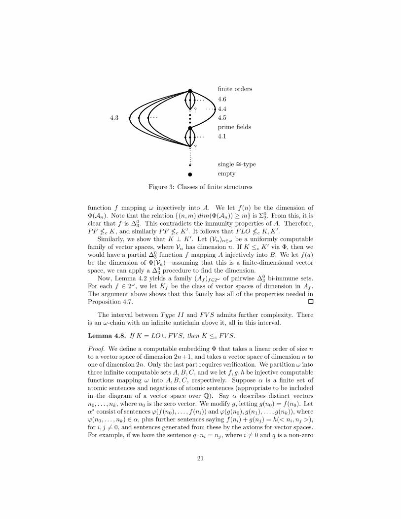
The results so far, for classes of finite structures, are summarized in Figure 3.Finite orders lie at the top, along with finite undirected graphs. Finite cyclicgroups, and finite simple groups lie there too. Prime fields lie strictly lower.The empty class obviously lies on the bottom. The classes consisting of copiesof a single finite structure lie just above that—equivalent to classes consistingof copies of a single computable structure. The numbers 4.3, 4.6, 4.1 refer topropositions showing the existence of large incomparable families, and 4.5 refersto the proposition producing a chain. The question marks indicate places wherethere may or may not be a class, lying below certain classes and above certainothers.

Of course, the structure is dramatically enriched when we also considerclasses containing infinite structures. We have seen that the class FV S of finitedimensional vector spaces over the rationals sits strictly above Type II. First,let us show that there are classes below FV S that are not below Type II.

Proposition 4.7. There is a family of classes (Kf )f∈2ω , such that for allf ∈ 2ω, Kf ≤c FV S and Kf is incomparable with Types I and II, and fordistinct f, g ∈ 2ω, Kf ⊥ Kg.

Proof. Let A, B ⊆ ω be a pair of ∆03 bi-immune sets, and let K, K ′ be the classes

of Q-vector spaces whose dimensions are members of A, B, respectively. We haveK, K ′ ≤c FV S, by Proposition 1.3. Next, we show that K, K ′ are incomparablewith Types I and II. By Corollary 2.7, no class containing vector spaces of twodifferent dimensions embeds in FLO. Therefore K, K ′ �c FLO, and it followsthat K, K ′ �c PF . Let (An)n∈ω be a uniformly computable sequence of fields,where An

∼= Fpn. Suppose PF ≤c K via Φ. From Φ, we will obtain a ∆0

3

20

✉ finite orders

r r r. . . 4.6

❜ ? . . . r4.4rrr

4.54.3

✉ prime fields

r r r. . . 4.1

❜ ?

r r r. . .

r

✉

single ∼=-type

empty

Figure 3: Classes of finite structures

function f mapping ω injectively into A. We let f(n) be the dimension ofΦ(An). Note that the relation {(n, m)|dim(Φ(An)) ≥ m} is Σ0

2. From this, it isclear that f is ∆0

3. This contradicts the immunity properties of A. Therefore,PF �c K, and similarly PF �c K ′. It follows that FLO �c K, K ′.

Similarly, we show that K ⊥ K ′. Let (Vn)n∈ω be a uniformly computablefamily of vector spaces, where Vn has dimension n. If K ≤c K ′ via Φ, then wewould have a partial ∆0

3 function f mapping A injectively into B. We let f(a)be the dimension of Φ(Va)—assuming that this is a finite-dimensional vectorspace, we can apply a ∆0

3 procedure to find the dimension.Now, Lemma 4.2 yields a family (Af )f∈2ω of pairwise ∆0

3 bi-immune sets.For each f ∈ 2ω, we let Kf be the class of vector spaces of dimension in Af .The argument above shows that this family has all of the properties needed inProposition 4.7.

The interval between Type II and FV S admits further complexity. Thereis an ω-chain with an infinite antichain above it, all in this interval.

Lemma 4.8. If K = LO ∪ FV S, then K ≤c FV S.

Proof. We define a computable embedding Φ that takes a linear order of size nto a vector space of dimension 2n+1, and takes a vector space of dimension n toone of dimension 2n. Only the last part requires verification. We partition ω intothree infinite computable sets A, B, C, and we let f, g, h be injective computablefunctions mapping ω into A, B, C, respectively. Suppose α is a finite set ofatomic sentences and negations of atomic sentences (appropriate to be includedin the diagram of a vector space over Q). Say α describes distinct vectorsn0, . . . , nk, where n0 is the zero vector. We modify g, letting g(n0) = f(n0). Letα∗ consist of sentences ϕ(f(n0), . . . , f(ni)) and ϕ(g(n0), g(n1), . . . , g(nk)), whereϕ(n0, . . . , nk) ∈ α, plus further sentences saying f(ni) + g(nj) = h(< ni, nj >),for i, j 6= 0, and sentences generated from these by the axioms for vector spaces.For example, if we have the sentence q ·ni = nj , where i 6= 0 and q is a non-zero

21

rational, then we obtain the sentence q · h(< ni, ni >) = h(< nj, hj >). We putinto Φ the pairs (α, ϕ), where α is as described, and ϕ is in the correspondingset α∗.

Proposition 4.9. There is a sequence of classes (Jn)n∈ω such that

LO ≤c J0 �c J1 �c J2 . . . ≤c FV S .

Proof. We define Jn to be the class containing all finite linear orders and allrational vector spaces of dimension at most 2n. If we wish, we can consider theseas structures in a single language, one that enables us to distinguish a linearorder from a vector space. Clearly, LO = J0. The proof that FV S �c LO (fromTheorem 2.6) shows that J1 �c LO. By Proposition 1.3, we have Jn ≤c Jn+1.Finally, if Jn+1 ≤c Jn via Φ, then Φ would map at least two isomorphismclasses of vector spaces to isomorphism classes of linear orders, which is againimpossible.

In Proposition 4.6, we obtained incomparable classes strictly between Types Iand II by adding to the class all of finite prime fields the linear orders of selectedsizes. Below, we use the same idea to obtain incomparable classes above all Jn

and below FV S.

Proposition 4.10. Let (Jn)n∈ω be as in Proposition 4.9. There exist pairwiseincomparable classes (Gf )f∈2omega such that for all n ∈ ω and all f ∈ 2ω, wehave Jn ≤c Gf ≤c FV S. (Then Jn �c Gf �c FV S.)

Proof. Each class Gn will contain all finite linear orders. We add vector spacesof selected dimensions so as to satisfy the following requirements.

R〈e,σ〉: for all f ⊇ σ 0, g ⊇ σ 1, We does not witness Gf ≤c Gg.

R′〈e,σ〉: for all f ⊇ σ 0, g ⊇ σ 1, We does not witness Gg ≤c Gf .

We have a list of all requirements. At each stage s, we have decided, for finitelymany pairs (i, n), whether to put vector spaces of dimension n in Gf , for f ⊇ τ ,for τ of length s. We write Gτ for the class reflecting the decisions made up tostage s. In the end, we will let Gf be the union of the sets Gτ , for τ ⊆ f .

We satisfy the requirements in order. At stage s + 1, we consider Require-ment s. Say this is R〈e,σ〉, and let Φ = We. Take n greater than the dimensionof any vector spaces considered so far. For all τ ⊇ σ 0 of length s + 1, we putinto Gτ the vector spaces of dimension n + i for i ≤ n. If Φ does not mapone of the newly added vector spaces to anything in FLO ∪ FV S, then therequirement is trivially satisfied. If Φ embeds Gτ into FLO∪FV S, then by theargument in Theorem 2.6 or Corollary 2.7, since Gτ contains vector spaces ofat least two different finite dimensions, Φ cannot map any vector space in Gτ

to a finite linear order. Thus, Φ must map one of the n + 1 new vector spacesto a vector space of dimension greater than n. We satisfy the requirement bykeeping the vector spaces of this dimension out of Gν , for all ν ⊇ σ 1 of lengths + 1.

22

✉ undirected graphs≡c?✉ linear orders

4.12✉ vector spaces

r r r...4.10

❜ ?rrr

4.9

✉ finite ordersrrr

4.11

✉ prime fieldsr r r. . .

4.7

✉ empty

Figure 4: Classes of structures, possibly infinite

There are other classes not below FV S. Of course, any class is embeddablein the class of infinite graphs. Also, we have an increasing sequence of classesthat is not below FV S. For each ordinal α < ω1, let LOα denote the set of wellorders of order type less than α.

Proposition 4.11. If α < β < ω1, then LOα �c LOβ. Also, for ω < α,LOα �c FV S.

Proof. If α < β, then Proposition 1.3 yields the fact that LOα ≤c LOβ . Thereare representatives of the order types in LOα forming a chain of structures oflength α. Then by Corollary 1.2, if α < β, Lβ � Lα, and if α > ω, thenLα � FV S.

This result also suffices to show that the class of infinite linear orders does notlie below the finite dimensional vector spaces. However, we have the following:

Proposition 4.12. If LO is the class of linear orders (possibly infinite), andFV S is the class of finite dimensional Q-vector spaces, then FV S ≤c LO.

Proof. Each vector space V will correspond to a substructure of ω·η, in which foreach n ≤ dim(V), we have densely many copies of the finite linear order of sizen, and also densely many copies of ω. Clearly if we can describe a computabletransformation that behaves this way, it will be well-defined and injective onisomorphism types.

Let B be the lexicographic ordering on Q × ω. We partition Q computablyinto dense subsets Q~a, corresponding to finite sequences ~a of natural numbers.Given a finite set α of atomic sentences and negations of atomic sentences de-scribing an n-tuple of vectors ~a, let α∗ describe the restriction of B to Q~a ×ω, ifα contains evidence that ~a is dependent, and Q~a × n, otherwise. Let Φ consistof the pairs (α, ϕ), where ϕ ∈ α∗.

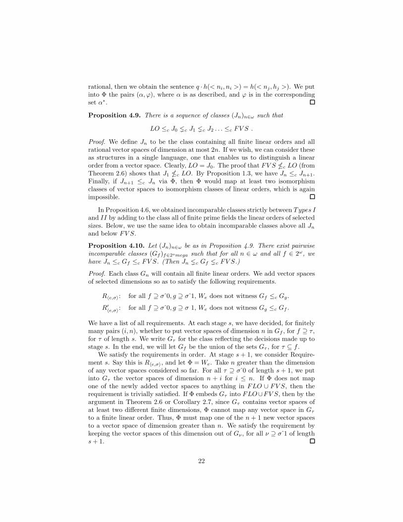
Thus, the situation when we include classes containing infinite structureslooks something like Figure 4. Undirected graphs lie on top. Linear orders

23

may or may not be equivalent to undirected graphs. Finite dimensional vectorspaces over Q lie strictly below linear orders, and finite linear orders lie strictlybelow vector spaces. The numbers 4.7, 4.10, etc., indicate the propositions beingillustrated.

5 Problems

In this section, we list some open problems.

Problem 1. Is the class of graphs computably equivalent to the class of linearorderings?

The class of graphs (including infinite as well as finite ones) lies at the top ofour partial ordering. Problem 1 asks whether there is a computable embeddingof graphs in linear orderings.

Problem 2. Is there a “natural” class K, consisting of finite structures of in-finitely many different isomorphism types, such that K is not computably equiv-alent to either finite prime fields or finite linear orderings? In particular, isthere a natural example of a class properly between these two?

We have results characterizing those classes that computably embed in thefinite prime fields, and also in the finite linear orderings. For classes that embedin the finite dimensional vector spaces over Q, we can give some necessaryconditions, but we have no characterization.

Problem 3. Characterize the classes K such that K ≤c FV S.

We have not entirely sorted out the differences between the definition of ≤c

that we chose and the two alternative definitions. We can show that the partialordering obtained from Definition 1′′ differs from ≤c. We do not know aboutthe partial ordering obtained from Definition 1′.

Problem 4. Is it true that for any classes of structures K, K ′, K ≤c K ′ iffthere is a computable operator Φ = ϕe of the kind in Definition 1′, taking A ∈ K

to B ∈ K ′ such that ϕD(A)e = χD(B), in a way that is well-defined and 1 − 1 on

isomorphism types?

References

[1] Ash, C. J., and J. F. Knight, Computable Structures and the Hyperarith-metical Hierarchy, Elsevier Science, 2000.

[2] Ash, C. J., and A. Nerode, “Intrinsically recursive relations”, in Aspects ofEffective Algebra, ed. by J. N. Crossley, Upside Down A Book Co., Steel’sCreek, Australia, pp. 26–41.

24

[3] Becker, H., and A. S. Kechris, The descriptive set theory of Polish groupactions, London Math. Soc. Lecture Note Series, vol. 232, CambridgeUniv. Press, 1996.

[4] Calvert, W., “The isomorphism problem for classes of computable fields”,preprint.

[5] Calvert, W., “The isomorphism problem for classes of computable Abeliangroups”, preprint.

[6] Dyment, E. Z., “Certain properties of the Medvedev lattice”,Matematiceskii Sbornik, vol. 101(143)(1976), pp. 360-379 (Russian); En-glish translation, Mathematics of the USSR Sbornik, vol. 30(1976), pp.321–340.

[7] Friedman, H., and L. Stanley, “A Borel reducibility theory for classes ofcountable structures”, J. Symb. Logic, vol. 54(1989), pp. 894–914.

[8] Goncharov, S. S., and J. F. Knight, “Computable structure and non-structure theorems”, Algebra and Logic, vol. 41(2002), pp. 351–373.

[9] Harizanov, V. S., “Some effects of Ash-Nerode and other decidabilityconditions on degree spectra”, Annals of Pure and Applied Logic, vol.55(1991), pp. 51–65.

[10] Hirschfeldt, D., B. Khoussainov, R. Shore and A. M. Slinko, “Degreespectra and computable dimensions in algebraic structures”, Annals ofPure and Appl. Logic, vol. 115(2002), pp. 71–113”.

[11] Hjorth, G., Classification and Orbit Equivalence Relations, Amer. Math.Society, 1999.

[12] Hjorth, G., and A. S. Kechris, “Recent developments in the theory ofBorel reducibility”, Fund. Math., vol. 170(2001), pp. 21–52.

[13] Hjorth, G., and A. S. Kechris, “Analytic equivalence relations and Ulm-type classifications”, J. Symb. Logic, vol. 60(1995), pp. 1273–1300.

[14] Knight, J. F., “Algebraic structure of classes under computable embed-ding”, in preparation.

[15] Marker, D., Model theory: An Introduction, Springer-Verlag, 2002.

[16] Medvedev, Yu. T, “Degrees of difficulty of the mass problems”, DokladyAkademii Nauk SSSR, vol. 104(1955), pp. 501–504 (Russian).

[17] Nies, A., “Undecidable fragments of elementary theories”, Algebra Uni-versalis, vol. 35(1996), pp. 8–33.

[18] Rabin, M. O., and D. Scott, “The undecidability of some simple theories”,preprint.

25

[19] Rogers, H., Theory of Recursive Functions and Effective Computability,MIT Press,1987.

[20] Simpson, S., and S. Binns, “Embeddings into the Medvedev and Muchniklattices of Π0

1 classes, preprint.

[21] Soare, R. I., Recursively Enumerable Sets and Degrees, Springer-Verlag,1987.

[22] Sorbi, A., “Some remarks on the algebraic structure of the Medvedevlattice”, J. Symb. Logic, vol. 55(1990), pp. 831–853.

26