Comparing Categorization Models

Comparing Categorization Models

Jeffrey N. Rouder andUniversity of Missouri—Columbia

Roger RatcliffThe Ohio State University

AbstractFour experiments are presented that competitively test rule- and exemplar-based models of humancategorization behavior. Participants classified stimuli that varied on a unidimensional axis into 2categories. The stimuli did not consistently belong to a category; instead, they were probabilisticallyassigned. By manipulating these assignment probabilities, it was possible to produce stimuli forwhich exemplar- and rule-based explanations made qualitatively different predictions.F. G. Ashbyand J. T. Townsend’s (1986) rule-based general recognition theory provided a better account of thedata than R. M. Nosofsky’s (1986) exemplar-based generalized context model in conditions in whichthe to-be-classified stimuli were relatively confusable. However, generalized context model provideda better account when the stimuli were relatively few and distinct. These findings are consistent withmultiple process accounts of categorization and demonstrate that stimulus confusion is a determiningfactor as to which process mediates categorization.

In this article we present an empirical paradigm to test different theories of categorizationbehavior. One theory we test is the exemplar-based theory in which categories are representedby sets of stored exemplars. Category membership of a stimulus is determined by similarityof the stimulus to these exemplars (e.g., Medin & Schaffer, 1978; Nosofsky, 1986, 1987,1991). An exemplar-based process relies on retrieval of specific trace-based informationwithout further abstraction; for example, a person is judged as “tall” if he or she is similar inheight to others who are considered “tall.” The other theory we test is rule-based or decision-bound theory. Decisions are based on an abstracted rule. The relevant space is segmented intoregions by bounds, and each region is assigned to a specific category (e.g., Ashby & Gott,1988; Ashby & Maddox, 1992, 1993; Ashby & Perrin, 1988; Ashby & Townsend, 1986;Trabasso & Bower, 1968). For example, a person might be considered tall if he or she isperceived as being over 6 ft (1.83 m). The essence of a rule-based process is that processingis based on greatly simplified abstractions or rules but not on the specific trace-basedinformation itself.

Both rule- and exemplar-based theories have gained a large degree of support in theexperimental literature. There are both exemplar-based models (e.g., generalized contextmodel; Nosofsky, 1986) and rule-based models (e.g., general recognition theory; Ashby &Gott, 1988; Ashby & Townsend, 1986) that can explain a wide array of behavioral data acrossseveral domains. Despite the many attempts to discriminate between these two explanations,there have been few decisive tests. Across several paradigms and domains, rule- and exemplar-based predictions often mimic each other.

Correspondence concerning this article should be addressed to Jeffrey N. Rouder, Department of Psychological Sciences, 210 McAlesterHall, University of Missouri, Columbia, MO 65211. E-mail: [email protected] N. Rouder, Department of Psychological Sciences, University of Missouri—Columbia; Roger Ratcliff, Psychology Department,The Ohio State University.

NIH Public AccessAuthor ManuscriptJ Exp Psychol Gen. Author manuscript; available in PMC 2006 March 20.

Published in final edited form as:J Exp Psychol Gen. 2004 March ; 133(1): 63–82.

NIH

-PA Author Manuscript

NIH

-PA Author Manuscript

NIH

-PA Author Manuscript

Roughly speaking, there are two main experimental paradigms for testing the above theoriesof categorization. One is a probabilistic assignment paradigm: Stimuli do not always belongto the same category. Instead, a stimulus is probabilistically assigned to categories by theexperimenter. Probabilistic assignment is meant to capture the uncertainty in many real-lifedecision-making contexts. For example, consider the problem of interpreting imperfectmedical tests. The test result may indicate the presence of a disease, but there is some chanceof a false positive. Examples of the use of probabilistic assignment in categorization tasksinclude the studies of Ashby and Gott (1988), Espinoza-Varas and Watson (1994), Kalish andKruschke (1997), McKinley and Nosofsky (1995), Ratcliff, Van Zandt, and McKoon (1999),and Thomas (1998). The other main paradigms for testing categorization models are transferparadigms. In these paradigms, participants first learn a set of stimulus–category assignments.Afterward, they are given novel stimuli to categorize, and the pattern of responses to thesenovel stimuli serves as the main dependent measure. Examples of the use of transfer includethe studies of Erickson and Kruschke (1998), Medin and Schaffer (1978), and Nosofsky,Palmeri, and McKinley (1994).

Both transfer and probabilistic assignment paradigms offer unique advantages anddisadvantages. In this article, we are concerned with probabilistic assignment. We first showthat the main drawback with probabilistic assignment is that in many paradigms, rule- andexemplar-based theories yield similar predictions—that is, they mimic each other. We thenpresent a novel method of assigning categories to stimuli that mitigates this problem andprovides for a differential test of the theories.

We report the results of four categorization experiments with simple, unidimensional stimuli.The results point to stimulus confusion as a salient variable. Stimulus confusion is the inabilityto identify stimuli in an absolute identification task. When stimuli are confusable, the resultsare consistent with rule-based models and inconsistent with exemplar models. When the stimuliare clear and distinct, however, the pattern favors an exemplar-based interpretation. The findingthat both exemplar- and rule-based processes may be used in the same task is compatible withrecent work in multiple-process and multiple-system frameworks (e.g., Ashby & Ell, 2002;Erickson & Kruschke, 1998; Nosofsky et al., 1994). The results provide guidance as to the typeof information that determines which system or process will mediate categorization.

Perhaps the best way to illustrate exemplar- and rule-based theories and their similarpredictions is with a simple experiment. Ratcliff and Rouder (1998) asked participants toclassify squares of varying luminance into one of two categories (denoted Category A andCategory B). For each trial, luminance of the stimulus was chosen from one of the twocategories. The stimuli from a given category were selected from a normal distribution on aluminance scale. The two categories had the same standard deviation but different means (seeFigure 1A). Feedback was given after each trial to tell the participants whether the decisionhad correctly indicated the category from which the stimulus had been drawn. Because thecategories overlapped substantially, participants could not be highly accurate. For example, astimulus of moderate luminance might have come from Category A on one trial and fromCategory B on another. But overall, dark stimuli tended to come from Category A and lightstimuli from Category B.

According to rule-based explanations, participants partition the luminance dimension intoregions and associate these regions with certain categories. The dotted line in Figure 1A denotesa possible criterion placement that partitions the luminance domain into two regions. If theparticipant perceives the stimulus as having luminance greater than the criterion, the participantproduces the Category B response; otherwise the participant produces the Category A response.A participant may not perfectly perceive the luminance of a stimulus, and perceptual noise canexplain gradations in the participant’s empirical response proportions. Alternatively, there may

Rouder and Ratcliff Page 2

J Exp Psychol Gen. Author manuscript; available in PMC 2006 March 20.

NIH

-PA Author Manuscript

NIH

-PA Author Manuscript

NIH

-PA Author Manuscript

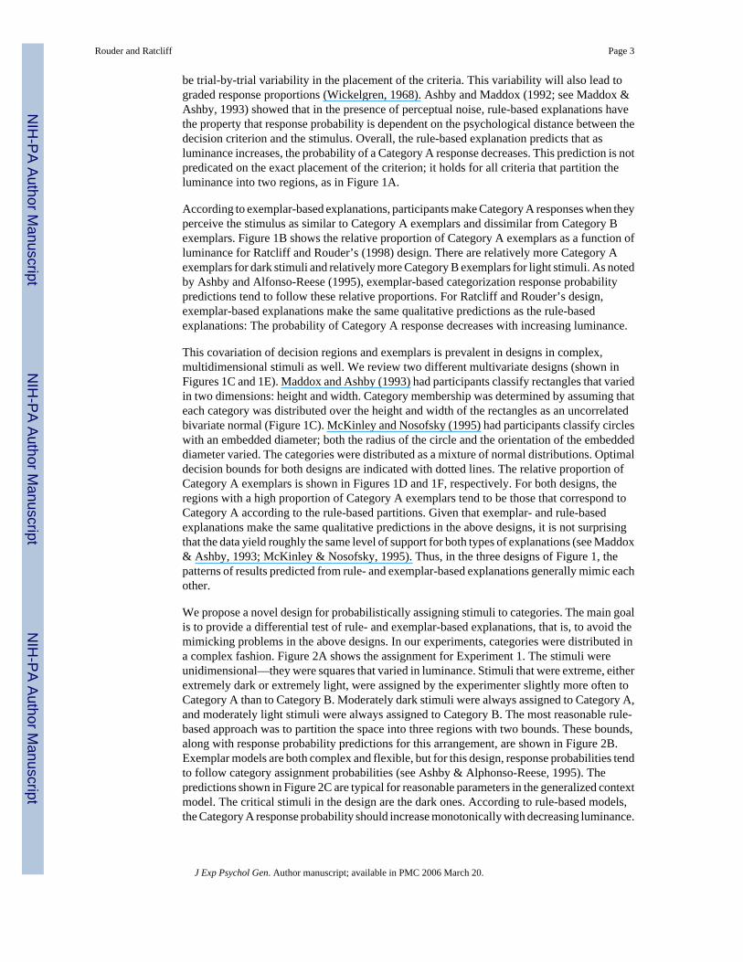
be trial-by-trial variability in the placement of the criteria. This variability will also lead tograded response proportions (Wickelgren, 1968). Ashby and Maddox (1992; see Maddox &Ashby, 1993) showed that in the presence of perceptual noise, rule-based explanations havethe property that response probability is dependent on the psychological distance between thedecision criterion and the stimulus. Overall, the rule-based explanation predicts that asluminance increases, the probability of a Category A response decreases. This prediction is notpredicated on the exact placement of the criterion; it holds for all criteria that partition theluminance into two regions, as in Figure 1A.

According to exemplar-based explanations, participants make Category A responses when theyperceive the stimulus as similar to Category A exemplars and dissimilar from Category Bexemplars. Figure 1B shows the relative proportion of Category A exemplars as a function ofluminance for Ratcliff and Rouder’s (1998) design. There are relatively more Category Aexemplars for dark stimuli and relatively more Category B exemplars for light stimuli. As notedby Ashby and Alfonso-Reese (1995), exemplar-based categorization response probabilitypredictions tend to follow these relative proportions. For Ratcliff and Rouder’s design,exemplar-based explanations make the same qualitative predictions as the rule-basedexplanations: The probability of Category A response decreases with increasing luminance.

This covariation of decision regions and exemplars is prevalent in designs in complex,multidimensional stimuli as well. We review two different multivariate designs (shown inFigures 1C and 1E). Maddox and Ashby (1993) had participants classify rectangles that variedin two dimensions: height and width. Category membership was determined by assuming thateach category was distributed over the height and width of the rectangles as an uncorrelatedbivariate normal (Figure 1C). McKinley and Nosofsky (1995) had participants classify circleswith an embedded diameter; both the radius of the circle and the orientation of the embeddeddiameter varied. The categories were distributed as a mixture of normal distributions. Optimaldecision bounds for both designs are indicated with dotted lines. The relative proportion ofCategory A exemplars is shown in Figures 1D and 1F, respectively. For both designs, theregions with a high proportion of Category A exemplars tend to be those that correspond toCategory A according to the rule-based partitions. Given that exemplar- and rule-basedexplanations make the same qualitative predictions in the above designs, it is not surprisingthat the data yield roughly the same level of support for both types of explanations (see Maddox& Ashby, 1993; McKinley & Nosofsky, 1995). Thus, in the three designs of Figure 1, thepatterns of results predicted from rule- and exemplar-based explanations generally mimic eachother.

We propose a novel design for probabilistically assigning stimuli to categories. The main goalis to provide a differential test of rule- and exemplar-based explanations, that is, to avoid themimicking problems in the above designs. In our experiments, categories were distributed ina complex fashion. Figure 2A shows the assignment for Experiment 1. The stimuli wereunidimensional—they were squares that varied in luminance. Stimuli that were extreme, eitherextremely dark or extremely light, were assigned by the experimenter slightly more often toCategory A than to Category B. Moderately dark stimuli were always assigned to Category A,and moderately light stimuli were always assigned to Category B. The most reasonable rule-based approach was to partition the space into three regions with two bounds. These bounds,along with response probability predictions for this arrangement, are shown in Figure 2B.Exemplar models are both complex and flexible, but for this design, response probabilities tendto follow category assignment probabilities (see Ashby & Alphonso-Reese, 1995). Thepredictions shown in Figure 2C are typical for reasonable parameters in the generalized contextmodel. The critical stimuli in the design are the dark ones. According to rule-based models,the Category A response probability should increase monotonically with decreasing luminance.

Rouder and Ratcliff Page 3

J Exp Psychol Gen. Author manuscript; available in PMC 2006 March 20.

NIH

-PA Author Manuscript

NIH

-PA Author Manuscript

NIH

-PA Author Manuscript

According to the exemplar-based models, the Category A response probability should decreasewith decreasing luminance.

Unlike previous designs, our relatively simple design, shown in Figure 2, has the ability todistinguish between exemplar- and rule-based explanations. The use of unidimensional stimulirestricts the complexity of exemplar- and rule-based models. Exemplar-based models ofmultidimensional stimuli often have adjustable attentional weights on the dimensions. Byselectively tuning these weights, the model becomes very flexible (see, e.g., Kruschke,1992;Nosofsky & Johansen, 2000). But with unidimensional stimuli, attention is set to thesingle dimension rather than tuned. Likewise, rule-based models are also constrained in onedimension; the set of plausible rules is greatly simplified.

Generalized Context Model (GCM)GCM is a well-known exemplar model that has had much success in accounting for data fromcategorization experiments (Nosofsky, 1986; Nosofsky & Johansen, 2000). According toGCM, participants make category decisions by comparing the similarity of the presentedstimulus to each of several stored category exemplars. In general, both the stimuli andexemplars are represented in a multidimensional space. But in Experiment 1, the stimuli variedon a single dimension: luminance. Therefore, we implement a version of the GCM in whichstimuli are represented on a unidimensional line termed perceived luminance.

In GCM performance is governed by the similarity of the perceived stimulus to storedexemplars. Each exemplar is represented as a point on the perceived-luminance line. Let xjdenote the perceived luminance of the jth exemplar, and let y denote the perceived luminanceof the presented stimulus. The distance between exemplar j and the stimulus on the perceived-luminance line is simply dj = |xj − y|. In GCM, the similarity of a stimulus to an exemplar j isrelated to this distance (see also Shepard, 1957, 1987) as

s j = exp( − λd jk), λ > 0. (1)

The exponent k describes the shape of the similarity gradient. Smaller values of k correspondto a sharper decrease in similarity with distance, whereas higher values correspond to ashallowed decrease. Two values of k are traditionally chosen: k = 1 corresponds to anexponential similarity gradient, and k = 2 corresponds to a Gaussian similarity gradient. In theanalyses presented here, we separately fit GCM with both the exponential (k = 1) and Gaussian(k = 2) gradients. Although the value of k is critically important in determining thecategorization of novel stimuli far in distance from previous exemplars (Nosofsky & Johansen,2000), it is less critical in the probabilistic assignment paradigms in which each stimulus isnearby to several exemplars. In our analyses, varying k only marginally affected model fits.The parameter λ is referred to as the sensitivity, and it describes how similarity linearly scaleswith distance. If λ is large, then similarity decreases rapidly with increasing distance. However,if λ is small, similarity decreases slowly with increasing distance.

The pivotal quantity in determining the response probabilities is the similarity of the stimulusto all of the exemplars. Each exemplar is associated with one or the other category. Let A beall of the exemplars associated with Category A, and let B be all of the exemplars associatedwith Category B. In GCM, the activation of a category is the sum of similarities of the stimulusto exemplars associated with that category. The activation of Category A to the stimulus isdenoted by a and given by

a = ∑j∈A

si. (2)

Rouder and Ratcliff Page 4

J Exp Psychol Gen. Author manuscript; available in PMC 2006 March 20.

NIH

-PA Author Manuscript

NIH

-PA Author Manuscript

NIH

-PA Author Manuscript

Likewise, the activation of Category B is denoted by b and given by

b = ∑j∈ℬ

s j. (3)

Response probabilities are based on the category activations. Let P(A) denote the probabilitythat the participant places the stimulus into Category A:

P(A) = aγ

aγ + bγ + φ, γ > 0. (4)

Parameter φ is a response bias. If φ is positive, then there is a response bias toward CategoryA. If φ is negative, then there is a response bias toward Category B. The parameter γ is theconsistency of response. If γ is large, responses tend to be consistent; stimuli are classified intoCategory A if a > b and into Category B if b > a. As γ decreases, responses are less consistent;participants sometimes choose Category B even when a > b. Parameter γ was not part of GCMin its original formulation (e.g., Nosofsky, 1986) but was added by Ashby and Maddox(1993) for generality.

In GCM, each trial generates a new exemplar (e.g., Nosofsky, 1986). The feedback on the trialdictates the category membership of the new exemplar, and the new exemplar’s position inpsychological space is that of the stimulus. In our experiments, we used eight differentluminance levels, and hence all of the exemplars fall on one of eight points on the perceivedluminance dimension. We denote the category assignment probability, the probability that theexperimenter assigns a stimulus with luminance i into Category A as φi. The proportion ofexemplars for Category A at a perceived luminance depends on the corresponding categoryassignment probability. Although this proportion may vary, as the number of trials increasesthis proportion converges to the category assignment probability. The category activations canbe expressed in terms of the category assignment probabilities (π). For luminance level i, thenumber of Category A exemplars is approximately Nπi, and each of these exemplars has asimilarity to the current stimulus given by si. Hence in the asymptotic limit of many trials,

a =∑iNπisi (5a)

and

b =∑iN (1 − πi)si. (5b)

The model specified by Equations 1, 4, 5a, and 5b was fit in the following experiments. Thethree free parameters were λ, γ, and π.

In subsequent exemplar models (e.g., Kruschke, 1992), exemplars could be forgotten. Althoughthe equations were derived for the case where exemplars are perfectly retained in memory,they still apply for this version as well, providing that forgetting occurs at an equal rate for allexemplars and exemplars are presented randomly.

General Recognition Theory (GRT)GRT is based on the assumption that people use decision rules to solve categorization problems.In GRT, perception is assumed to be inherently variable. For example, the perceived luminanceof a stimulus is assumed to vary from trial to trial, even for the same stimulus. In general, theperceptual effects of stimuli in GRT can be represented in a multidimensional psychologicalspace. For the squares of varying luminance in Experiment 1, the appropriate psychological

Rouder and Ratcliff Page 5

J Exp Psychol Gen. Author manuscript; available in PMC 2006 March 20.

NIH

-PA Author Manuscript

NIH

-PA Author Manuscript

NIH

-PA Author Manuscript

space is the perceived luminance line. Participants use decision criteria to partition theperceived luminance line into line segments. Each segment is associated with a category, andthe categorization response on a given trial depends on which segment contains the stimulus’sperceived luminance.

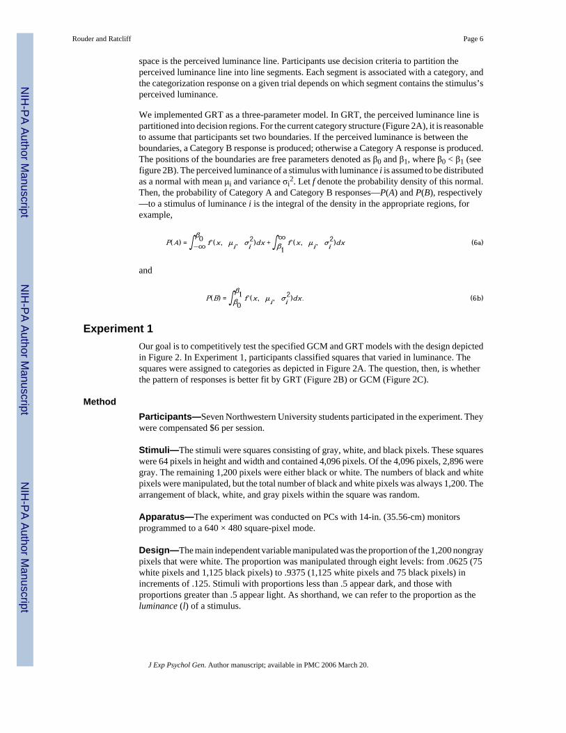
We implemented GRT as a three-parameter model. In GRT, the perceived luminance line ispartitioned into decision regions. For the current category structure (Figure 2A), it is reasonableto assume that participants set two boundaries. If the perceived luminance is between theboundaries, a Category B response is produced; otherwise a Category A response is produced.The positions of the boundaries are free parameters denoted as β0 and β1, where β0 < β1 (seefigure 2B). The perceived luminance of a stimulus with luminance i is assumed to be distributedas a normal with mean μi and variance σi

2. Let f denote the probability density of this normal.Then, the probability of Category A and Category B responses—P(A) and P(B), respectively—to a stimulus of luminance i is the integral of the density in the appropriate regions, forexample,

P(A) = ∫−∞β0 f (x, μi, σi

2)dx + ∫β1∞f (x, μi, σi

2)dx (6a)

and

P(B) = ∫β0β1 f (x, μi, σi

2)dx. (6b)

Experiment 1Our goal is to competitively test the specified GCM and GRT models with the design depictedin Figure 2. In Experiment 1, participants classified squares that varied in luminance. Thesquares were assigned to categories as depicted in Figure 2A. The question, then, is whetherthe pattern of responses is better fit by GRT (Figure 2B) or GCM (Figure 2C).

MethodParticipants—Seven Northwestern University students participated in the experiment. Theywere compensated $6 per session.

Stimuli—The stimuli were squares consisting of gray, white, and black pixels. These squareswere 64 pixels in height and width and contained 4,096 pixels. Of the 4,096 pixels, 2,896 weregray. The remaining 1,200 pixels were either black or white. The numbers of black and whitepixels were manipulated, but the total number of black and white pixels was always 1,200. Thearrangement of black, white, and gray pixels within the square was random.

Apparatus—The experiment was conducted on PCs with 14-in. (35.56-cm) monitorsprogrammed to a 640 × 480 square-pixel mode.

Design—The main independent variable manipulated was the proportion of the 1,200 nongraypixels that were white. The proportion was manipulated through eight levels: from .0625 (75white pixels and 1,125 black pixels) to .9375 (1,125 white pixels and 75 black pixels) inincrements of .125. Stimuli with proportions less than .5 appear dark, and those withproportions greater than .5 appear light. As shorthand, we can refer to the proportion as theluminance (l) of a stimulus.

Rouder and Ratcliff Page 6

J Exp Psychol Gen. Author manuscript; available in PMC 2006 March 20.

NIH

-PA Author Manuscript

NIH

-PA Author Manuscript

NIH

-PA Author Manuscript

Procedure—Each trial began with the presentation of a large gray background of 320 × 200square pixels. Then, 500 ms later, the square of black, gray, and white pixels was placed in thecenter of the gray background. The square remained present until 400 ms after the participanthad responded. Participants pressed the z key to indicate that the square belonged in CategoryA and the / key to indicate that the square belonged in Category B. Category assignmentprobability is depicted in Figure 2A. Very black and very white stimuli (e.g., stimuli withextreme proportions) were assigned to Category A with a probability of π = .6. Moderatelyblack stimuli were always assigned to Category A (π = 1.0), and moderately white stimuli werealways assigned to Category B (π = 0). If the participant’s response did not match the categoryassignment, an error message was presented after the participant’s response, and it remainedon the monitor for 400 ms. A block consisted of 96 such trials. After each block, the participantwas given a short break. There were 10 blocks in a session, and each session took about 35min to complete. Participants were tested until the response probabilities were fairly stableacross three consecutive sessions; this took between four and six sessions. Stability wasassessed by visual inspection of the day-to-day plots or response proportions.

Instructions—Participants were instructed that category assignment was a function of thenumber of black and white pixels but not the arrangement of black, white, and gray pixels.They were told to learn which stimulus belonged to which category by paying careful attentionto the feedback. They were also informed that the feedback was probabilistic in nature, andthat they could not avoid receiving error messages on some trials. They were instructed to tryto keep errors to a minimum. To explain probabilistic feedback, we provided participants withthe following example from reading medical x-rays: A doctor sees a suspicious spot on an x-ray and orders a biopsy. The biopsy reveals a malignancy. In this case the doctor has correctlyclassified the x-ray as “problematic.” The same doctor sees another x-ray from a differentpatient with the same type of suspicious spot. But the biopsy on this second patient reveals nomalignancy; the spot is due to naturally occurring variation in tissue density. Here the doctorhas classified the same stimulus (the suspicious spot) as “problematic” but is in error as thereis no malignancy. Because life is variable, a response in a situation at one time is correct butthe same response at another time is wrong. Participants were told that there were “tendencies”;certain luminances were more likely to belong to one category than the other. Participants werealso told that the order of presentation was random and that only the luminance on the currenttrial determined the probability that the stimulus belongs to one or the other category. If aparticipant’s data for the first session showed a monotonic pattern in which dark stimuli wereplaced into Category A and light stimuli into Category B, the participant was instructed thatthere was a better solution and was asked to find it.

ResultsOne of the 7 participants withdrew after three sessions. The data are analyzed for each of theremaining 6 participants individually and are from the last three sessions. Response probability,the probability that the participant classified a stimulus into Category A, is plotted as a functionof luminance in Figure 3. Each of the six graphs corresponds to data from a different participant.Empirical response proportions are plotted with circles and error bars (which denote standarderrors1). The lines are model fits, to be discussed later.

Overall, there are some aspects of the response probability data that were common to severalparticipants. Four of the 6 participants (B.G., N.C., S.E.H., and S.B.) produced response

1The standard errors in the figures were calculated by computing response proportions on a block-by-block basis (a block is 96 trials andconsists of 12 observations at each luminance level). The variability of these response proportions across blocks was then used incalculating standard errors. This method was implemented because it is conceivable that true underlying response probabilities are notconstant across different blocks or sessions. Factors that could increase the variability in response probability are variability in attentionand strategy. The current method assumes that response proportions are constant within a block but vary across blocks.

Rouder and Ratcliff Page 7

J Exp Psychol Gen. Author manuscript; available in PMC 2006 March 20.

NIH

-PA Author Manuscript

NIH

-PA Author Manuscript

NIH

-PA Author Manuscript

probabilities that were similar to the rules pattern in Figure 2B. Extreme stimuli (very dark orvery light) were more often classified in Category A and moderate stimuli in Category B.Participants V.B. and L.T. differed from the other 4 in that their Category A responseproportions were higher for moderately dark stimuli than for the darkest stimuli. ParticipantV.B.’s data resemble the exemplar pattern in Figure 2C. Participant L.T.’s data do not resembleeither the rule or the exemplar pattern. To better gain insight on how these patterns can beinterpreted in a competitive test, we fit GRT and GCM.

Model-Based Analyses of Experiment 1Parameter Estimation—We fit models to data by minimizing the chi-square goodness-of-fit statistic with repeated application of the Simplex algorithm (Nelder & Mead, 1965). TheSimplex algorithm is a local minimization routine and is susceptible to settling on a localminimum. To help find a global minimum, we constructed an iterative form of Simplex. Thebest fitting parameters from one cycle were perturbed and then used as the starting value forthe next cycle. Cycling continued until 500 such cycles resulted in the same minimum. Theamount of perturbation between cycles increased each time the routine yielded the sameminimum as the previous cycle.

There are some difficulties introduced by adopting a chi-square fit criterion having to do withsmall predicted frequencies. For several response patterns, reasonable parameters yieldexceedingly small predictions, for example, .01 of a count. These small numeric values werethe denominator of the chi-square statistic and led to unstable values. It is often difficult tominimize functions with such instabilities. As a compromise, the denominator of the chi-squarestatistic was set to the larger of 5 or the predicted frequency value.2 Although this modificationallows for more robust and stable parameter estimates, it renders the chi-square testinappropriate for formal tests. In this report, we use the chi-square fit statistic as both adescriptive index and a metric for assessing the relative fit of comparable models rather thanas an index of the absolute goodness of fit of a model. We still report p < .05 significance valuesthroughout for rough comparisons of fit.

Experiment 1A: Scaling Luminance To fit both GCM and GRT, it is necessary to scalethe physical domain (luminance) into a psychological domain (perceived luminance). Toprovide data for scaling luminance, we performed Experiment 1A, which consisted of anabsolute-identification and a similarity-ratings task.

Participants Three Northwestern University students served as participants and received $8in compensation. Two of the 3 participants had also participated, about 6 months earlier, inExperiment 1.

2As this minimum value of the denominator is decreased, responses with probability near 0 or 1 have increasingly greater leverage indetermining the fit. To see how this works, consider the case in which the predicted response probability is .5 versus the case where itis .001 (assuming no minimum denominator). There are about 300 observations per condition in the reported experiments. Therefore,the predicted frequencies are 150 and .3 for predicted probabilities of .5 and .001, respectively. Because these predicted frequencies enterin the denominator of the chi-square fit statistic, the net effect is a differential weighting of the squared difference between observed andpredicted frequencies. In the case for which the predicted frequency is .3, the squared differences are weighted by a factor of 500 morethan the case for which the predicted value is 150. Having a minimum value eliminates the case in which squared differences from smallpredicted response frequencies receive such extreme weightings. In the current example, the minimum value of 5 would be used in thechi-square denominator instead of the predicted frequency of .3. In this case, the relative weighting of the extreme response probabilityis only 30 times that of intermediary response probability. An alternative approach is to minimize the root-mean-square error of theresponse proportion predictions (see Massaro, Cohen, Campbell, & Rodriguez, 2001; Rouder & Gomez, 2001). This approach placesequal weights on deviations from all response probabilities. The disadvantage of this approach is that such a method fails to take intoaccount that extreme response proportions are associated with smaller error bars. The current technique of using a chi-square fit statisticwith a minimum strives at a compromise. Extreme responses with smaller standard errors carry greater weight in determining modelparameters than moderate response proportions. Because a minimum is used in the denominator, extreme response proportions do notfully determine the fit.

Rouder and Ratcliff Page 8

J Exp Psychol Gen. Author manuscript; available in PMC 2006 March 20.

NIH

-PA Author Manuscript

NIH

-PA Author Manuscript

NIH

-PA Author Manuscript

Stimuli Stimuli were the eight square patches of varying luminances used in Experiment 1.

Design and procedure Each participant first performed the similarity-ratings task and thenperformed the absolute-identification task. In the similarity-ratings task, the 3 participants weregiven pairs of square stimuli and asked to judge the similarity of the pair using a 10-point scale.Participants observed all possible pairings five times. After completing the similarity task,participants were given an absolute-identification task in which they had to identify the eightdifferent luminance levels by selecting a response from 1 (darkest) to 8 (brightest). After eachresponse, participants were shown the correct response. Participants observed three blocks of120 trials each. The last two blocks (240 trials, or 30 trials per stimulus) were retained forconstructing perceived luminance scales.

Scale Construction—The data from the 3 participants in Experiment 1A were used toconstruct five scales of perceived luminance (presented below). Multiple scales wereconstructed so that we could determine whether a failure of a model was due to misspecificationof scale. To foreshadow, when a model failed, it failed for all applicable scales. Hence, thesefailures may be attributed to structural properties of the models rather than scalemisspecifications.

Similarity-Ratings Scale for GCM In GCM, categorization decisions are determined bysimilarity. Data from the similarity task were converted to distance (d = ln[s − 1]; Shepard,1957, 1987) and scaled with a classic multidimensional scaling routine. Scaling was done oneach of the 3 participants’ data separately. For each participant, the first dimension accountedfor an overwhelming amount of variance—eigenvalues of the first dimension were more thanseven times greater than those of the second. Therefore, a unidimensional scale is justified,and the coordinates on the first dimension were averaged across participants to produce theSimilarity-Ratings Scale.

Absolute-Identification Scale for GCM The absolute-identification data can also be used toconstruct a perceived luminance scale. To construct such a scale for GCM, we followedNosofsky (1986) and used a variant of Luce’s similarity choice model (Luce, 1959, 1963).3

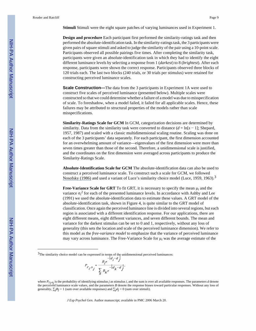
Free-Variance Scale for GRT To fit GRT, it is necessary to specify the mean μi and thevariance σi

2 for each of the presented luminance levels. In accordance with Ashby and Lee(1991) we used the absolute-identification data to estimate these values. A GRT model of theabsolute-identification task, shown in Figure 4, is quite similar to the GRT model ofclassification. Once again the perceived luminance line is divided into several regions, but eachregion is associated with a different identification response. For our applications, there areeight different means, eight different variances, and seven different bounds. The mean andvariance for the darkest stimulus can be set to 0 and 1, respectively, without any loss ofgenerality (this sets the location and scale of the perceived luminance dimension). We refer tothis model as the free-variance model to emphasize that the variance of perceived luminancemay vary across luminance. The Free-Variance Scale for μi was the average estimate of the

3The similarity choice model can be expressed in terms of the unidimensional perceived luminances:

Pri,s j=

Bie−|di−d j|

∑k

Bke−|dk−d j| ,

where Pri,sj is the probability of identifying stimulus j as stimulus i, and the sum is over all available responses. The parameters d denotethe perceived luminance scale values, and the parameters B denote the response biases toward particular responses. Without any loss ofgenerality, ∑jBj = 1 (sum over available responses) and ∑jdj = 0 (sum over stimuli).

Rouder and Ratcliff Page 9

J Exp Psychol Gen. Author manuscript; available in PMC 2006 March 20.

NIH

-PA Author Manuscript

NIH

-PA Author Manuscript

NIH

-PA Author Manuscript

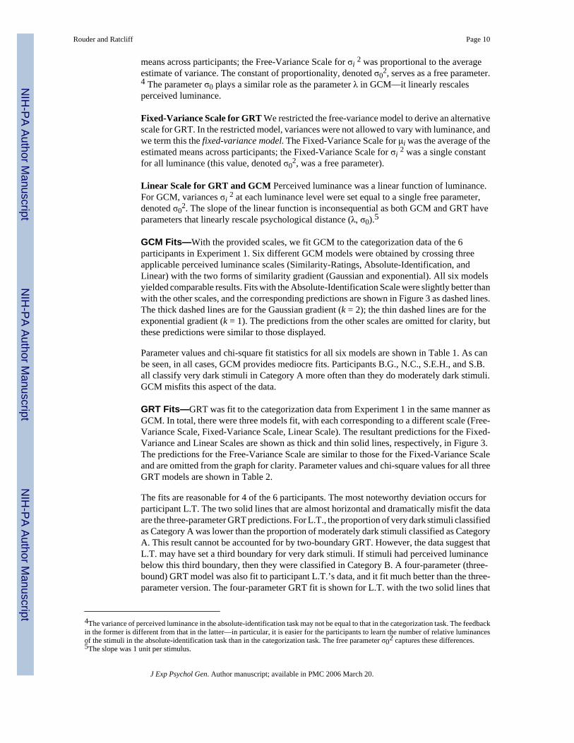
means across participants; the Free-Variance Scale for σi 2 was proportional to the averageestimate of variance. The constant of proportionality, denoted σ0

2, serves as a free parameter.4 The parameter σ0 plays a similar role as the parameter λ in GCM—it linearly rescalesperceived luminance.

Fixed-Variance Scale for GRT We restricted the free-variance model to derive an alternativescale for GRT. In the restricted model, variances were not allowed to vary with luminance, andwe term this the fixed-variance model. The Fixed-Variance Scale for μi was the average of theestimated means across participants; the Fixed-Variance Scale for σi 2 was a single constantfor all luminance (this value, denoted σ0

2, was a free parameter).

Linear Scale for GRT and GCM Perceived luminance was a linear function of luminance.For GCM, variances σi 2 at each luminance level were set equal to a single free parameter,denoted σ0

2. The slope of the linear function is inconsequential as both GCM and GRT haveparameters that linearly rescale psychological distance (λ, σ0).5

GCM Fits—With the provided scales, we fit GCM to the categorization data of the 6participants in Experiment 1. Six different GCM models were obtained by crossing threeapplicable perceived luminance scales (Similarity-Ratings, Absolute-Identification, andLinear) with the two forms of similarity gradient (Gaussian and exponential). All six modelsyielded comparable results. Fits with the Absolute-Identification Scale were slightly better thanwith the other scales, and the corresponding predictions are shown in Figure 3 as dashed lines.The thick dashed lines are for the Gaussian gradient (k = 2); the thin dashed lines are for theexponential gradient (k = 1). The predictions from the other scales are omitted for clarity, butthese predictions were similar to those displayed.

Parameter values and chi-square fit statistics for all six models are shown in Table 1. As canbe seen, in all cases, GCM provides mediocre fits. Participants B.G., N.C., S.E.H., and S.B.all classify very dark stimuli in Category A more often than they do moderately dark stimuli.GCM misfits this aspect of the data.

GRT Fits—GRT was fit to the categorization data from Experiment 1 in the same manner asGCM. In total, there were three models fit, with each corresponding to a different scale (Free-Variance Scale, Fixed-Variance Scale, Linear Scale). The resultant predictions for the Fixed-Variance and Linear Scales are shown as thick and thin solid lines, respectively, in Figure 3.The predictions for the Free-Variance Scale are similar to those for the Fixed-Variance Scaleand are omitted from the graph for clarity. Parameter values and chi-square values for all threeGRT models are shown in Table 2.

The fits are reasonable for 4 of the 6 participants. The most noteworthy deviation occurs forparticipant L.T. The two solid lines that are almost horizontal and dramatically misfit the dataare the three-parameter GRT predictions. For L.T., the proportion of very dark stimuli classifiedas Category A was lower than the proportion of moderately dark stimuli classified as CategoryA. This result cannot be accounted for by two-boundary GRT. However, the data suggest thatL.T. may have set a third boundary for very dark stimuli. If stimuli had perceived luminancebelow this third boundary, then they were classified in Category B. A four-parameter (three-bound) GRT model was also fit to participant L.T.’s data, and it fit much better than the three-parameter version. The four-parameter GRT fit is shown for L.T. with the two solid lines that

4The variance of perceived luminance in the absolute-identification task may not be equal to that in the categorization task. The feedbackin the former is different from that in the latter—in particular, it is easier for the participants to learn the number of relative luminancesof the stimuli in the absolute-identification task than in the categorization task. The free parameter σ02 captures these differences.5The slope was 1 unit per stimulus.

Rouder and Ratcliff Page 10

J Exp Psychol Gen. Author manuscript; available in PMC 2006 March 20.

NIH

-PA Author Manuscript

NIH

-PA Author Manuscript

NIH

-PA Author Manuscript

fit the data reasonably well. For the remaining participant, V.B., GRT fit well but failed tocapture the small downturn for the darkest stimuli.

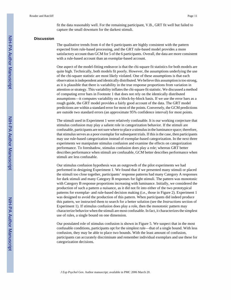
DiscussionThe qualitative trends from 4 of the 6 participants are highly consistent with the patternexpected from rule-based processing, and the GRT rule-based model provides a moresatisfactory account than GCM for 5 of the 6 participants. Overall, the data are more consistentwith a rule-based account than an exemplar-based account.

One aspect of the model-fitting endeavor is that the chi-square fit statistics for both models arequite high. Technically, both models fit poorly. However, the assumptions underlying the useof the chi-square statistic are most likely violated. One of these assumptions is that eachobservation is independent and identically distributed. We believe this assumption is too strong,as it is plausible that there is variability in the true response proportions from variation inattention or strategy. This variability inflates the chi-square fit statistic. We discussed a methodof computing error bars in Footnote 1 that does not rely on the identically distributedassumptions—it computes variability on a block-by-block basis. If we use the error bars as arough guide, the GRT model provides a fairly good account of the data. The GRT modelpredictions are within a standard error for most of the points. Conversely, the GCM predictionsare outside two standard errors (an approximate 95% confidence interval) for most points.

The stimuli used in Experiment 1 were relatively confusable. It is our working conjecture thatstimulus confusion may play a salient role in categorization behavior. If the stimuli areconfusable, participants are not sure where to place a stimulus in the luminance space; therefore,that stimulus serves as a poor exemplar for subsequent trials. If this is the case, then participantsmay use rule-based categorization instead of exemplar-based categorization. In the next threeexperiments we manipulate stimulus confusion and examine the effects on categorizationperformance. To foreshadow, stimulus confusion does play a role; whereas GRT betterdescribes performance when stimuli are confusable, GCM better describes performance whenstimuli are less confusable.

Our stimulus confusion hypothesis was an outgrowth of the pilot experiments we hadperformed in designing Experiment 1. We found that if we presented many stimuli or placedthe stimuli too close together, participants’ response patterns had many Category A responsesfor dark stimuli and many Category B responses for light stimuli. The pattern was monotonicwith Category B response proportions increasing with luminance. Initially, we considered theproduction of such a pattern a nuisance, as it did not fit into either of the two prototypicalpatterns for exemplar- and rule-based decision making (i.e., those in Figure 2). Experiment 1was designed to avoid the production of this pattern. When participants did indeed producethis pattern, we instructed them to search for a better solution (see the Instructions section ofExperiment 1). If stimulus confusion does play a role, then the monotonic pattern maycharacterize behavior when the stimuli are most confusable. In fact, it characterizes the simplestuse of rules, a single bound on one dimension.

Our postulated role of stimulus confusion is shown in Figure 5. We suspect that in the mostconfusable conditions, participants opt for the simplest rule—that of a single bound. With lessconfusion, they may be able to place two bounds. With the least amount of confusion,participants can accurately discriminate and remember individual exemplars and use these forcategorization decisions.

Rouder and Ratcliff Page 11

J Exp Psychol Gen. Author manuscript; available in PMC 2006 March 20.

NIH

-PA Author Manuscript

NIH

-PA Author Manuscript

NIH

-PA Author Manuscript

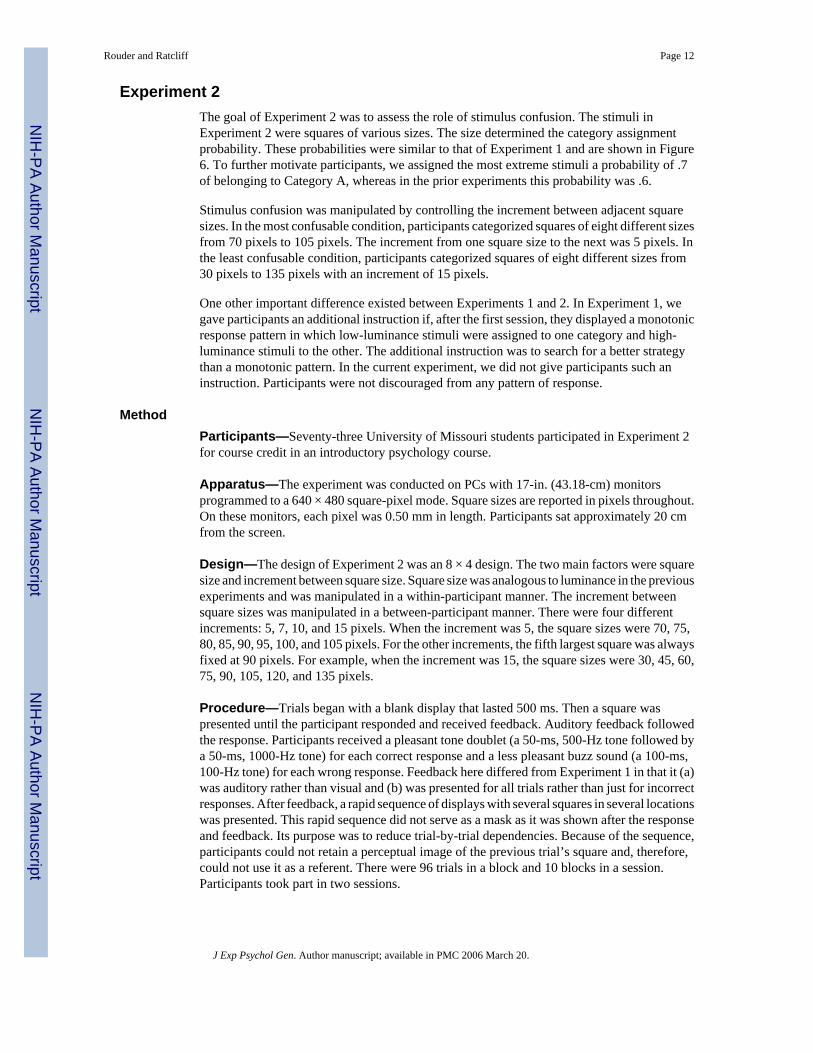
Experiment 2The goal of Experiment 2 was to assess the role of stimulus confusion. The stimuli inExperiment 2 were squares of various sizes. The size determined the category assignmentprobability. These probabilities were similar to that of Experiment 1 and are shown in Figure6. To further motivate participants, we assigned the most extreme stimuli a probability of .7of belonging to Category A, whereas in the prior experiments this probability was .6.

Stimulus confusion was manipulated by controlling the increment between adjacent squaresizes. In the most confusable condition, participants categorized squares of eight different sizesfrom 70 pixels to 105 pixels. The increment from one square size to the next was 5 pixels. Inthe least confusable condition, participants categorized squares of eight different sizes from30 pixels to 135 pixels with an increment of 15 pixels.

One other important difference existed between Experiments 1 and 2. In Experiment 1, wegave participants an additional instruction if, after the first session, they displayed a monotonicresponse pattern in which low-luminance stimuli were assigned to one category and high-luminance stimuli to the other. The additional instruction was to search for a better strategythan a monotonic pattern. In the current experiment, we did not give participants such aninstruction. Participants were not discouraged from any pattern of response.

MethodParticipants—Seventy-three University of Missouri students participated in Experiment 2for course credit in an introductory psychology course.

Apparatus—The experiment was conducted on PCs with 17-in. (43.18-cm) monitorsprogrammed to a 640 × 480 square-pixel mode. Square sizes are reported in pixels throughout.On these monitors, each pixel was 0.50 mm in length. Participants sat approximately 20 cmfrom the screen.

Design—The design of Experiment 2 was an 8 × 4 design. The two main factors were squaresize and increment between square size. Square size was analogous to luminance in the previousexperiments and was manipulated in a within-participant manner. The increment betweensquare sizes was manipulated in a between-participant manner. There were four differentincrements: 5, 7, 10, and 15 pixels. When the increment was 5, the square sizes were 70, 75,80, 85, 90, 95, 100, and 105 pixels. For the other increments, the fifth largest square was alwaysfixed at 90 pixels. For example, when the increment was 15, the square sizes were 30, 45, 60,75, 90, 105, 120, and 135 pixels.

Procedure—Trials began with a blank display that lasted 500 ms. Then a square waspresented until the participant responded and received feedback. Auditory feedback followedthe response. Participants received a pleasant tone doublet (a 50-ms, 500-Hz tone followed bya 50-ms, 1000-Hz tone) for each correct response and a less pleasant buzz sound (a 100-ms,100-Hz tone) for each wrong response. Feedback here differed from Experiment 1 in that it (a)was auditory rather than visual and (b) was presented for all trials rather than just for incorrectresponses. After feedback, a rapid sequence of displays with several squares in several locationswas presented. This rapid sequence did not serve as a mask as it was shown after the responseand feedback. Its purpose was to reduce trial-by-trial dependencies. Because of the sequence,participants could not retain a perceptual image of the previous trial’s square and, therefore,could not use it as a referent. There were 96 trials in a block and 10 blocks in a session.Participants took part in two sessions.

Rouder and Ratcliff Page 12

J Exp Psychol Gen. Author manuscript; available in PMC 2006 March 20.

NIH

-PA Author Manuscript

NIH

-PA Author Manuscript

NIH

-PA Author Manuscript

Participants were told not to dwell on any one trial but not to go so fast as to make carelessmotor errors. As in Experiment 1, participants were given a short story about probabilisticoutcomes in medical tests. Unlike Experiment 1, they were not instructed about the reliabilityof feedback across the range of square sizes.

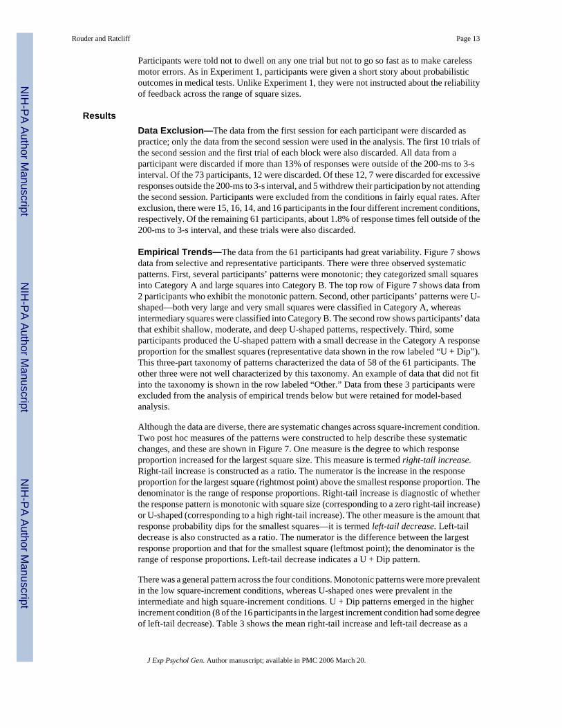
ResultsData Exclusion—The data from the first session for each participant were discarded aspractice; only the data from the second session were used in the analysis. The first 10 trials ofthe second session and the first trial of each block were also discarded. All data from aparticipant were discarded if more than 13% of responses were outside of the 200-ms to 3-sinterval. Of the 73 participants, 12 were discarded. Of these 12, 7 were discarded for excessiveresponses outside the 200-ms to 3-s interval, and 5 withdrew their participation by not attendingthe second session. Participants were excluded from the conditions in fairly equal rates. Afterexclusion, there were 15, 16, 14, and 16 participants in the four different increment conditions,respectively. Of the remaining 61 participants, about 1.8% of response times fell outside of the200-ms to 3-s interval, and these trials were also discarded.

Empirical Trends—The data from the 61 participants had great variability. Figure 7 showsdata from selective and representative participants. There were three observed systematicpatterns. First, several participants’ patterns were monotonic; they categorized small squaresinto Category A and large squares into Category B. The top row of Figure 7 shows data from2 participants who exhibit the monotonic pattern. Second, other participants’ patterns were U-shaped—both very large and very small squares were classified in Category A, whereasintermediary squares were classified into Category B. The second row shows participants’ datathat exhibit shallow, moderate, and deep U-shaped patterns, respectively. Third, someparticipants produced the U-shaped pattern with a small decrease in the Category A responseproportion for the smallest squares (representative data shown in the row labeled “U + Dip”).This three-part taxonomy of patterns characterized the data of 58 of the 61 participants. Theother three were not well characterized by this taxonomy. An example of data that did not fitinto the taxonomy is shown in the row labeled “Other.” Data from these 3 participants wereexcluded from the analysis of empirical trends below but were retained for model-basedanalysis.

Although the data are diverse, there are systematic changes across square-increment condition.Two post hoc measures of the patterns were constructed to help describe these systematicchanges, and these are shown in Figure 7. One measure is the degree to which responseproportion increased for the largest square size. This measure is termed right-tail increase.Right-tail increase is constructed as a ratio. The numerator is the increase in the responseproportion for the largest square (rightmost point) above the smallest response proportion. Thedenominator is the range of response proportions. Right-tail increase is diagnostic of whetherthe response pattern is monotonic with square size (corresponding to a zero right-tail increase)or U-shaped (corresponding to a high right-tail increase). The other measure is the amount thatresponse probability dips for the smallest squares—it is termed left-tail decrease. Left-taildecrease is also constructed as a ratio. The numerator is the difference between the largestresponse proportion and that for the smallest square (leftmost point); the denominator is therange of response proportions. Left-tail decrease indicates a U + Dip pattern.

There was a general pattern across the four conditions. Monotonic patterns were more prevalentin the low square-increment conditions, whereas U-shaped ones were prevalent in theintermediate and high square-increment conditions. U + Dip patterns emerged in the higherincrement condition (8 of the 16 participants in the largest increment condition had some degreeof left-tail decrease). Table 3 shows the mean right-tail increase and left-tail decrease as a

Rouder and Ratcliff Page 13

J Exp Psychol Gen. Author manuscript; available in PMC 2006 March 20.

NIH

-PA Author Manuscript

NIH

-PA Author Manuscript

NIH

-PA Author Manuscript

function of condition. Although these measures are continuous in nature, there are manyparticipants who scored near the bounds of one and zero. In this case, nonparametric statisticsare useful in assessing trends. Each participant was ranked on both measures. Table 3 alsoshows the mean ranks for each increment condition (each mean rank is from 58 participants).Both right-tail increase and left-tail decrease increase with increment. The direction andmonotonicity of these trends support the hypothesis that stimulus confusion affectscategorization behavior with a progression from simple rules to more complicated rules toexemplar storage with increased stimulus confusion. To assess the statistical significance ofthese trends, we performed a planned comparison in which ranks in the two low-incrementconditions were compared against ranks in the high-increment conditions with a Mann–Whitney U test (Hayes, 1994). The changes were significant (right-tail increase: U = 242.5,p ≤ .05; left-tail decrease: U = 296, p ≤ .05). To further test the working hypothesis about therole of stimulus confusion, we conducted model-based analyses.

Model-Based Analyses of Experiment 2To perform model analyses, it is necessary to scale the square sizes into a psychological spaceof perceived size. Fifteen University of Missouri undergraduates performed an absolute-identification task similar to that of Experiment 1A for this purpose. With these absolute-identification data, Absolute-Identification, Free-Variance, and Fixed-Variance Scales wereconstructed as previously discussed.

Four GCM models were fit to the categorization data of Experiment 2. These models wereobtained by crossing the two perceived-size scales (Absolute-Identification Scale and LinearScale) with the similarity gradients (exponential and Gaussian). Although all four model fitswere fairly similar, GCM with the Gaussian similarity gradient and Absolute-IdentificationScale fit the best for three of the four increment conditions. To keep the graphs less cluttered,only these predictions are shown (Figure 7, dashed lines). GCM models not displayed yieldedqualitatively similar predictions and misfit aspects of the data in the same manner as thedisplayed predictions. Three GRT models were fit (Fixed-Variance Scale, Free-Variance Scale,and Linear Scale). The fit with the Linear Scale was best in each of the four incrementconditions. The corresponding predictions are shown (Figure 7, solid lines). GRT fits withFixed-Variance and Free-Variance Scales were similar to that with the Linear Scale; misfitsoccurred at the same points and in the same direction.

The results of the model-based analyses are fairly straightforward. If a participant displayed amonotonic pattern with smaller squares placed in Category A and larger squares placed inCategory B, then only the GRT model provided a satisfactory fit. GRT in these cases reducedto a one-bound model as the estimated upper bounds were much greater than the largest squaresize. The fits to the U-shaped pattern were more complex. If the U-shaped pattern was relativelyshallow without extreme response proportions, then GRT tended to fit better than GCM.However, if the U-shaped pattern was relatively deep with extreme response proportions, thenboth GCM and GRT fit well. If there was some degree of left-tail decrease, then GCMoutperformed GRT.

Overall, GRT fit better in the small increment, high stimulus-confusion conditions, asparticipants exhibit monotonic and U-shaped patterns. But in the lowest stimulus-confusioncondition, a substantial number of participants demonstrate left-tail decrease, and theseparticipants’ data are best fit with GCM. Figure 8 graphically depicts these trends. It showsthe distributions of the chi-square fit statistics as empirical cumulative distribution functions.The chi-square values of each participant were ordered from smallest to largest; the logarithmsof these values are plotted on the x-axis. The y-axis is the proportion of fits less than or equalto a certain value. The cumulative distribution functions of chi-square statistics from well-fitting models tend to dominate those from poor-fitting models. In the top panel, for a square

Rouder and Ratcliff Page 14

J Exp Psychol Gen. Author manuscript; available in PMC 2006 March 20.

NIH

-PA Author Manuscript

NIH

-PA Author Manuscript

NIH

-PA Author Manuscript

size increment of 5, the distribution of chi-square values from the three GRT models is shownas solid lines. These dominate the four dashed lines from the four GCM models. Thisdominance indicates a better fit for GRT than for GCM. But for an increment of 15, none ofthe three GRT models dominates the four GCM models. For this condition, 10 participants arebetter fit by GCM, whereas 6 are better fit by GRT. Those participants better fit with GCMtend to have substantial left-tail decrease.

DiscussionParticipants exhibited a wide variety of categorization behavior. Even so, the empirical trendsand model-based analysis tell a consistent story: Stimulus confusion affects categorizationperformance. When the stimuli are most confusable, participants tend to produce a monotonicpattern that is better fit by GRT. These good-fitting GRT models have a single bound. Asstimulus confusion is lessened, more participants tend to produce more U-shaped patterns.These U-shaped patterns also tend to be better fit with GRT. In the least confusable conditions,there is a left-tail decrease for some participants, and these patterns are better fit by GCM thanby GRT. The main caveat is that there is much individual variability. A set of stimuli that areconfusable for one participant may not be for another. Hence, these two participants may usedifferent strategies. Our finding that different individuals are better fit by different models isnot too surprising and is in accordance with the results of Nosofsky et al. (1994) and Thomas(1998).

We suspect that stimuli in the least confusable condition were still somewhat confusable. Thereis a well-known processing limitation in absolute identification with unidimensional stimuli.Pollack (1952) found that participants were only 80% accurate in identifying 14 tones between500 Hz and 1000 Hz. Pollack then increased the range (14 tones were placed between 500 Hzand 5000 Hz) but still obtained only 80% accuracy. This result, along with several similar onesin different unidimensional domains, suggests that there is a mnemonic limitation in the abilityto identify unidimensional stimuli that cannot be abrogated by increasing the physicalseparation between stimuli (see Miller, 1956; Shiffrin & Nosofsky, 1994). Rouder (2001) foundthat absolute identification with line lengths is fairly limited with six lines. These studies, takentogether, indicate that there may be some mnemonic confusion for a set of eight square sizes,even for arbitrarily large increments. Stimulus confusion reflects contributions from perceptualvariability and mnemonic limits. In short, stimulus confusion is tantamount to the ability toabsolutely identify stimuli. If stimuli cannot be identified in an absolute sense, then there is atleast some degree of stimulus confusion. To further explore the role of stimulus confusion, wemade the stimuli less confusable in Experiment 3 by using only four well-spaced squares. Thisstimulus set yields reliable absolute identification and greatly reduced stimulus confusion.

Experiment 3Experiment 3 was designed to assess categorization performance when stimulus confusion isgreatly reduced. Reduction in stimulus confusion was obtained by using four well-spacedsquares. The category assignment probabilities for the squares are shown in Figure 9. Althoughthis assignment pattern differs from the previous experiment, it retains the important propertyof providing for differential predictions. Exemplar-based models predict that there should bemore Category A responses to Stimulus II than to Stimulus I because there are more CategoryA exemplars for Stimulus II. Rule-based models predict a bound between Stimulus III andStimulus IV. Stimuli smaller than the bound (Stimuli I, II, and III) should be classified intoCategory A on a majority of trials, whereas Stimulus IV, the sole stimulus larger than the bound,should be classified into Category B on a majority of the trials. Stimulus II is closer to thebound than is Stimulus I. Accordingly, there should be more Category A responses for StimulusI than for Stimulus II.

Rouder and Ratcliff Page 15

J Exp Psychol Gen. Author manuscript; available in PMC 2006 March 20.

NIH

-PA Author Manuscript

NIH

-PA Author Manuscript

NIH

-PA Author Manuscript

MethodParticipants—Six University of Missouri students participated in the experiment. They werecompensated $7.50 per experimental session. They each participated in two sessions.

Stimuli and Design—The size of the square was manipulated (within block) through fourlevels: 15 pixels, 35 pixels, 60 pixels, and 90 pixels. The category assignment probabilities forStimuli I, II, II, and IV were .583, .767, .933, and .067, respectively.

Procedure—The procedure was nearly identical to that of Experiment 2. Participantsobserved twice as many trials per stimulus as in Experiment 2, as there were half as manystimuli.

ResultsAnalysis was on data from the second session. The first 10 responses and the first response ofeach block were discarded. About .3% of the remaining responses fell outside of the 200-msto 3-s interval. These responses were also discarded. The resulting response proportions forthe four size conditions are shown in Figure 10. All 6 participants classified Stimulus II inCategory A more often than they did Stimulus I, hence qualitatively violating the decision-bound model. Consider as a null hypothesis that participants were as likely to classify StimulusI into Category A as they were to classify Stimulus II. The probability that all 6 participantswould classify Stimulus I into Category A more often than they did Stimulus II under this nullhypothesis is less than .016. Hence, we can generalize the result even though it was obtainedwith a relatively small sample size.

Model-Based Analyses of Experiment 3Scaling Luminance—To fit both GCM and GRT, it is necessary to scale the stimuli into apsychological space. Three undergraduates served as participants in exchange for course credit.They performed similarity-ratings and absolute-identification tasks similar to those inExperiment 1A. A Similarity-Ratings Scale was constructed with the same method as inExperiment 1A. We were not successful in scaling the stimuli with the absolute-identificationtask and could not produce Absolute-Identification, Free-Variance, or Fixed-Variance Scales.The reason for this failure is that participants performed near ceiling (.98) in the absolute-identification task. The lack of confusions made distance estimates unreliable. Of course, thisis expected, as the stimuli were so few in number and distinct. The use of a single task-basedmeasure is not problematic, as the model-based conclusions in the previous experiments havebeen robust to differences in the scales.

In addition to the Similarity-Ratings Scale, two other scales were constructed. One was theLinear Scale, in which perceived size was linear with veridical size. The other scale was linearwith stimulus’s ordinal position (i.e., 1, 2, 3, 4) and is termed the Ordinal-Position Scale. Inthe previous experiments, the Linear Scale and the Ordinal-Position Scale were the same, assquare size (luminance) was linearly related to ordinal position. In this experiment, the squareswere not sized in a linear fashion; instead, the difference between consecutive squares increasedwith square size.

GRT Fits—The optimal solution from the GRT perspective is to use a single bound (it shouldbe set between Stimuli III and IV). We used this solution as guidance and implemented a one-bound, two-parameter GRT model. Two such models were fit: one with the Linear Scale andthe other with the Ordinal-Position Scale. The model fared poorly with both scales (chi-squaregoodness-of-fit values are shown in Table 4). The GRT predictions (with the Linear Scale) areshown as solid lines in Figure 10. The predictions for the Ordinal-Position Scale are similar inthat they misfit the same points and in the same directions.

Rouder and Ratcliff Page 16

J Exp Psychol Gen. Author manuscript; available in PMC 2006 March 20.

NIH

-PA Author Manuscript

NIH

-PA Author Manuscript

NIH

-PA Author Manuscript

GCM Fits—We used a two-parameter version of GCM. This was to equate the number ofparameters in both GCM and GRT. Model comparisons are easier to make if both models havethe same number of parameters. A two-parameter GCM model was implemented by settingresponse bias (φ) to zero. Six GCM models were fit; these were obtained by crossing the threescales (Similarity-Ratings, Linear, and Ordinal-Position) with the two similarity gradients(exponential and Gaussian). It mattered little which GCM models we fit. GCM predictions(Gaussian similarity and Linear Scale) are shown as dashed lines in Figure 10, and the chi-square goodness-of-fit values are shown in Table 4. As can be seen, GCM does a better job offitting the data than GRT. This relation holds regardless of the scale or similarity gradient.

DiscussionThe results and model analysis show that Experiment 3 is more consistent with GCM thanGRT. The most salient difference between this experiment and the previous ones is the reducednumber of stimuli and subsequent reduced stimulus confusion. As is consistent with theprevious results, this reduction in confusion allows for the placement of exemplars and a shiftto exemplar-based categorization.

It may be possible to account for the data with GRT in a post hoc fashion. Perhaps participantsadopted a second decision bound below the smallest square size. If this is the case, due toperceptual variability, some of the presentations from the smallest square stimulus may fallbelow this bound and elicit a Category B response. This two-bound GRT model can accountfor the left-tail decrease exhibited by the participants. But such an explanation seemsimplausible as it postulates a decision bound in a region of the space in which no stimuli arepresented. The following experiment was designed to further test the stimulus confusionhypothesis. It was also designed in a manner to preclude a bound placement outside the stimulusrange.

Experiment 4The results of the preceding experiments provide evidence for the hypothesis that stimulusconfusion plays a role in determining the mode of categorization. The goal of Experiment 4 isto provide further evidence for the working hypothesis, and stimulus confusion was againmanipulated. In contrast to Experiment 2, the main manipulation of stimulus confusion wasthe addition of a line with tick marks under the to-be-classified square. With this line, an astuteobserver could determine the size of the square without perceptual variability and presumablywithout much stimulus confusion. To draw comparisons, there was a control condition in whichthe tick-marked line was not provided.

Participants categorized squares of six different sizes into two categories. The categoryassignment probabilities are shown in Figure 11. In this paradigm, the appropriate strategy inthe decision-bound approach is to place a single bound. If the perceived size of a square issmaller than the bound, the square should be classified into Category A; otherwise it shouldbe classified into Category B. The predictions for the GCM model are qualitatively moreflexible; it can account for the monotonic pattern. But GCM can account for a pattern GRTcannot: the one with more moderate classification probabilities for the second and fifth stimulithan for the third and fourth stimuli. One of the advantages of this design is that the extremestimuli also have extreme categorization probabilities. Hence, it is unreasonable to think thatparticipants adopted bounds outside of the range of presented square sizes. According to thestimulus-confusion hypothesis, the data will be differentially better accounted with GCM thanGRT in the experimental condition (with the tick-marked line placed under stimuli) than in thecontrol condition.

Rouder and Ratcliff Page 17

J Exp Psychol Gen. Author manuscript; available in PMC 2006 March 20.

NIH

-PA Author Manuscript

NIH

-PA Author Manuscript

NIH

-PA Author Manuscript

MethodParticipants—Twenty-four University of Missouri undergraduate students served asparticipants for course credit in an introductory psychology course. Fourteen served in theexperimental condition, 9 served in the control condition, and 1 was eliminated because theresulting data showed no variation across different square sizes.

Design—The design was a 6 × 2 mixed-factorial design. Square size was manipulated withinparticipants. The six square sizes ranged from 10 pixels to 160 pixels in increments of 30 pixels.There were two levels of confusion: experimental condition, with the tick-marked line, andcontrol condition, without the tick-marked line. Confusion was manipulated betweenparticipants.

Procedure—The procedure was identical to that in Experiments 2 and 3 with the followingexception. In the experimental condition, the line with the tick mark appeared 10 pixels belowthe bottom edge of the to-be-classified square. The line was centered under the square.Participants in the experimental condition were instructed to use the line in making theircategorization decisions. There were equal numbers of all six stimuli. As before, sessionsconsisted of 10 blocks of 96 trials each.

ResultsData exclusion followed previous guidelines. The first 50 trials were discarded as practicetrials, as was the first trial of each block. Two participants were discarded for excessiveresponses outside of the 200-ms to 3-s interval. For the remaining participants, 2.0% of theresponse times fell outside of the interval, and these trials were discarded. The averagedcategorization proportions are shown in Figure 12. In contrast with the previous three studies,data from individual participants were sufficiently similar to warrant averaging. In the controlcondition, participants’ categorization proportions followed a monotonic pattern even thoughthe assigned categorization proportions were nonmonotonic. By contrast, in the experimentalcondition, participants’ categorization proportions reflected the nonmonotonicities in theassigned categorization probabilities. Analysis of individuals (Figures 13 and 14) shows thatall 9 participants in the control condition exhibited strict monotonicity in response proportionas a function of size, whereas 10 of the 12 participants in the experimental condition exhibitedat least one violation of monotonicity.

Scale Construction and Model-Based AnalysesThe previous experiments indicate that the Linear Scale provides for a fair and representativecomparison of the models with these stimuli. It was the only scale used in fitting the data fromExperiment 4. As in Experiment 3, we fit a two-parameter version of each categorization model.For GRT, there was a single bound, and for GCM, bias was set to zero.6 We fit two GCMmodels (one for each gradient) and one GRT model. Predictions are shown in Figures 13 and14. The displayed GCM fit (dashed lines) is for the Gaussian similarity gradient; predictionsfrom the exponential similarity gradient are nearly identical and are omitted for clarity.

The distributions of the chi-square fit statistics across participants are plotted as cumulativedistribution functions in Figure 15. Overall, GCM fits the data better than GRT in bothconditions. The difference in fits is much larger in the experimental condition than in the control

6We encountered a new difficulty in fitting GCM in this experiment. The model fit well, but for some participants it yielded a very highestimate for parameter γ. This in itself is not problematic, as parameter γ denotes the degree of stochasticity in the response. High valuesindicate that participants are very consistent in their answers. To speed convergence, we capped the estimate of γ to be less than or equalto a value of 500, which is exceptionally high.

Rouder and Ratcliff Page 18

J Exp Psychol Gen. Author manuscript; available in PMC 2006 March 20.

NIH

-PA Author Manuscript

NIH

-PA Author Manuscript

NIH

-PA Author Manuscript

condition. Only GCM can account for the nonmonotonic pattern that resulted from adding thetick-marked line.

It was expected that GCM would fit better than GRT in the experimental condition as therewas little stimulus confusion, but GCM also fit better in the control condition. This is notsurprising, as the stimuli are relatively low in number and distinct. In support of the hypothesis,GCM differentially fit better when stimulus confusion was reduced by the addition of the tick-marked line.

As noted previously, GCM is more flexible than GRT for this design, and flexibility has becomea topical issue in model selection (e.g., Kass & Raftery, 1995; Myung & Pitt, 1997; Pitt, Myung,& Zhang, 2003). Although this difference in flexibility makes model selection complicated incases in which both GRT and GCM qualitatively account for the data, it is of little concern forcases in which one model clearly fails. Therefore, whereas the small advantage of GCM overGRT in the control condition may be accounted for in terms of increased flexibility, the largeadvantage of GCM over GRT in the experimental condition may not.

General DiscussionWe have presented a paradigm for contrasting rule- and exemplar-based theories ofcategorization behavior. The paradigm is based on probabilistic assignment—and theassignment is complex and nonlinear. Importantly, categorization theories yield differentialpredictions in this paradigm. The results from the four experiments, taken together, yieldconsistent findings. First, for any given experiment, there is a large degree of individualvariability. Often, some participants produce data that are better fit by GCM, and others producedata that are better fit by GRT. This degree of participant-level variability is present in similarstudies (e.g., Nosofsky et al., 1994; Thomas, 1998). Second, and more important, the degreeto which GCM and GRT held varied systematically with stimulus confusion. GRT betterdescribes categorization with confusable stimuli; GCM better describes categorization withdistinct stimuli. The rationale offered is that when the stimuli are too confusable, placementof exemplars may not be sufficiently reliable for use on subsequent categorization trials. InExperiment 1, there was a moderate degree of stimulus confusion, mostly due to the use ofeight, unidimensional stimuli. GRT fit better than GCM. In Experiment 2, the distance betweenstimuli was manipulated. Although the data were variable, the evidence suggests that ruleswere used in the more confusable conditions but that rules and exemplars were used in the leastconfusable condition. We speculate that stimuli in the least confusable condition were stillconfusable—owing to the nature of processing limits with unidimensional stimuli. InExperiment 3, stimulus confusion was reduced by using only four well-spaced stimuli, and aspredicted, GCM better described categorization performance. Finally, in Experiment 4,stimulus confusion was reduced by presenting participants a tick-marked line such that theycould “measure” the stimuli. Although GCM fit better than GRT in both conditions, itdifferentially fit better in the reduced-confusion condition.

There are a number of models derived from GCM and GRT. Kruschke’s (1992) attentionlearning covering map (ALCOVE) is a neural network instantiation of GCM that models trial-by-trial learning. As participants reach asymptotic performance, GCM and ALCOVE yieldequivalent predictions. ALCOVE is challenged in the conditions in which GCM fails, notablywhen there is a moderate to large degree of stimulus confusion. Another model derived fromGCM is Nosofsky and Palmeri’s exemplar-based random walk (EBRW; Nosofsky & Palmeri,1997). EBRW makes qualitatively similar accuracy predictions to GCM in the limit ofasymptotic performance and is challenged by results GCM fails to predict. GRT hasgeneralizations, too. Ashby (2000) recently proposed a stochastic version of GRT that accounts

Rouder and Ratcliff Page 19

J Exp Psychol Gen. Author manuscript; available in PMC 2006 March 20.

NIH

-PA Author Manuscript

NIH

-PA Author Manuscript

NIH

-PA Author Manuscript

for response choice and response time. But this model is also challenged by the data from thelow stimulus-confusion conditions that follow exemplar-like patterns.

Dual-Process/Dual-System Categorization ModelsRecently, a number of researchers have advanced dual-process or dual-system categorizationmodels, models that posit two distinct processing modes for categorization. Nosofsky andcolleagues’ rule-plus-exception model (RULEX) is an example of a categorization model thathas both rule- and exemplar-based mechanisms (Nosofsky et al., 1994; Nosofsky & Palmeri,1998). According to RULEX, people first use simple, one-bound, dimensional rules to solvecategorization problems. If this strategy fails (i.e., if the participants believe they are makingan unacceptable proportion of errors), then participants adopt more complex conjunctions ofsimple rules. If this strategy fails, participants may supplement the rules by memorizing a fewexceptions in addition to the rules. RULEX can certainly account for the rulelike behaviorobserved in the experiments. But RULEX can also store exemplars and does so in a regionwhere rules produce too many errors. For example, it is within the spirit of RULEX to positexemplars for the extreme stimuli in Experiments 1 and 2—those with intermediate categoryassignment probabilities. In this manner, the model can qualitatively predict the exemplar-based data pattern. The only difficulty with RULEX is that there are no mechanisms to explainthe effects of stimulus confusion. One extension would have the choice of strategy (whetherto use simple rules, complex rules, or complex rules and exemplars) be dependent on stimulusconfusion. With very confusable stimuli, participants expect and tolerate more errors.Therefore, they may be content with only single-criterion rules. With moderately confusablestimuli, the tolerance for error decreases and the rules become more complex. With the lessconfusable stimuli, tolerance of errors is at its lowest, and the rules are supplemented withexceptions.

Erickson and Kruschke’s (1998) ATRIUM is another dual-process model of categorization.According to ATRIUM, participants use a rule-based module and an exemplar-based modulein parallel. On each trial, both modules compute category activations. A gate then determinesthe net influence of each module on the categorization decision. The gate is complex and isdifferentially set depending on the stimulus. For stimuli that are correctly classified by a simpledimensional rule, the gate favors the rule-based module; for stimuli that are correctly classifiedby an exemplar, the gate favors the exemplar-based module. ATRIUM incorporates learningmechanisms for training the gate and the modules. ATRIUM can theoretically account for allthree of the patterns presented in Figure 5. The single-bound solution (left panel) can beobtained by biasing the gate toward the rule-based mechanism. The exemplar-based solution(right panel) can be obtained by biasing the gate toward the exemplar-based mechanism. Thetwo-bound solution (center panel) can be obtained by using the simple rule represented by theleft bound and Category A exemplars for large square sizes (high luminance). The model isrichly parameterized, and there has yet to be a discussion of how specific learning parametersinfluence the emergence of predictive patterns. It is unclear whether the model could predictthe observed data.

ATRIUM, like RULEX, does not explicitly account for changes in classification data as afunction of stimulus confusion. Erickson and Kruschke (2002) provide an informal discussionof when rules are induced in ATRIUM. They state that rules are more likely to be inducedwhen the categorization problem is easier. Their argument goes as follows: Learning anapplicable rule is a beneficial strategy because if the rule is correct, then the participant haslearned the correct categorization strategy for several stimuli at once. Learning exemplars,while guaranteed to provide good categorization decisions for repeated stimuli, takes moretime, effort, and resources. In ATRIUM, learning is competitive; learning rules reduce theability to learn with exemplars and vice versa. Erickson and Kruschke argue that in the face of

Rouder and Ratcliff Page 20

J Exp Psychol Gen. Author manuscript; available in PMC 2006 March 20.

NIH

-PA Author Manuscript

NIH

-PA Author Manuscript

NIH

-PA Author Manuscript

this trade-off, participants should adopt rules for easy tasks (presumably those without stimulusconfusion) while relying on exemplars for difficult tasks (presumably those with stimulusconfusion).

Although we agree that learning both rules and exemplars will happen differentially acrossdifferent conditions, our account differs from that of Erickson and Kruschke (2002). We findthat exemplars are used for easy tasks whereas rules are used for more difficult ones. Ourexplanation is in accordance with Erickson and Kruschke’s observation that learning rules doessimplify categorization problems greatly. We suspect that because rules do simplify problems,they will be invoked when simplification is needed most, that is, when the task is difficult (withstimulus confusion). In cases in which stimuli are distinct, then, eventually exemplars may bereliably placed and used.

Ashby and colleagues (e.g., Ashby, Alfonso-Reese, Turken, & Waldron, 1998; Ashby & Ell,2001, 2002; Waldron & Ashby, 2001) have also been persuasive in proposing a two-systemcategorization model. One system, the explicit system, makes categorization decisions basedon simple, easy-to-verbalize rules. An example of an easy-to-verbalize rule comes fromMaddox and Ashby’s (1993) categorization problem for rectangles (see Figure 1C of thisarticle). This problem can be solved with the verbal rule of classifying rectangles with heightsgreater than widths into Category A and those with widths greater than heights into CategoryB. The explicit system corresponds well with theories that participants are forming and testingdifferent explicit hypotheses to solve the categorization task. Participants consciously maintainthese rules in the explicit system; its locus is assumed to be in the frontal lobes. The secondcategorization system is the implicit system. Participants do not have conscious access to thissystem; its locus is in the basal ganglia. The implicit system works through slower, Hebbian-like, associative learning. It can learn solutions that need not be stated verbally. For example,it is impossible to verbalize a rule that captures a reasonable decision bound in McKinley andNosofsky’s (1995) experiment depicted in Figure 1E. This problem is solved with the implicitsystem and not the verbal explicit system. Ashby et al. (1998) have implemented this two-system theory as both a neuropsychological model and a formal mathematical model. Bothimplementations are termed competition between verbal and implicit systems (COVIS).

COVIS receives support from several domains. First, it accounts for dissociations in behavioraleffects. For example, the time to learn a categorization problem depends on whether the rulecan be verbalized (Maddox & Ashby, 1993). It also accounts for the differential effect ofStroop-like interference (Waldron & Ashby, 2001). This interference occurs for simplecategorization problems with verbalizable solutions but not for more complex ones withnonverbalizable solutions. A second line of support comes from dissociations among clinicalpopulations. Patients with basal ganglia disease, frontal lobe damage, and temporal lobedamage show different patterns of categorization impairment (Ashby & Ell, 2001, 2002;Knowlton, Mangels, & Squire, 1996; Knowlton & Squire, 1993; Knowlton, Squire et al.,1996; Maddox & Filoteo, 2001). Finally, neuroimaging studies have shown differentialpatterns in brain activation depending on the particular categorization task (Patalano, Smith,Jonides, & Koeppe, 2002; Poldrack, Prabhakaran, Seger, & Gabrielli, 1999; Reber, Stark, &Squire, 1998). Each of these lines of support, however, has been critiqued in some part onlogical grounds (e.g., Nosofsky & Johansen, 2000; Nosofsky & Zaki, 1998; Zaki & Nosofsky,2002).

The question of interest is whether the exemplar pattern of results in Experiments 3 and 4challenges COVIS, the formal implementation of Ashby’s dual-system theory. Technically, itdoes. Both systems are rule based, and neither can account for the observed behavior that isinconsistent with GRT. But Ashby and Ell (2001, 2002) present an informal alternative—theybelieve it is possible to consciously remember a few stimulus–category pairings. Of course,

Rouder and Ratcliff Page 21

J Exp Psychol Gen. Author manuscript; available in PMC 2006 March 20.

NIH

-PA Author Manuscript

NIH

-PA Author Manuscript

NIH

-PA Author Manuscript

remembering a stimulus–category pairing, whether conscious or not, is an exemplar process.In essence, then, Ashby and Ell describe a three-system account: an explicit rule system, animplicit rule system, and an exemplar system for a small number of stimulus–category pairings.For unidimensional stimuli, our proposal about the role of exemplars is fairly concordant withthat of Ashby and Ell’s alternative. If there are a few distinct stimuli, categorization will bemediated by exemplars. Alternatively, if there are several confusable stimuli, categorization ismediated by one or both of the rule-based systems. In the next section, we discuss the case ofcomplex multidimensional stimuli. For these cases, our approach differs from that of Ashbyand Ell.

Stimulus DimensionalityOur results were obtained in a unidimensional paradigm. Although this paradigm is simple andinformative, the complexity of the results makes generalization complicated. In this article, weused the term stimulus confusion as a proxy for absolute identification. It is well known thatidentification with unidimensional and low-dimensional stimuli is limited, even after extensivepractice (Hartman, 1954; Miller, 1956; Rouder, Morey, Cowan, & Pfaltz, in press; Shiffrin &Nosofsky, 1994). For example, people can identify only seven or so tones and line lengths.According to our results, exemplar-based results hold only if there are less than a handful ofunidimensional stimuli. If there are more than seven, then participants may not be able to placeexemplars and may only use rules. The number of stimuli people can recognize in a domaindoes indeed increase with additional dimensions. There are a variety of estimates of how manytwo-dimensional stimuli people can identify. Although these estimates vary depending onprocedure and stimuli, the limit of identification is less than 25 stimuli (Eriksen & Hake,1955; Lockhead, 1970). This limit is greater than that with unidimensional stimuli, but it isstill a severe limit. We hypothesize that exemplar-based performance will be seen below thelimit, whereas rule-based performance will be seen above it. Accordingly, rule-basedperformance will be observed for categorization problems with stimulus confusion—cases inwhich there are many low-dimensional stimuli such as simple geometric shapes, colors, orpatches of luminance.

The limitations in identification can be contrasted to domains in which stimuli are complex.People can identify as many as 100,000 different words (Landauer, 1986) and probably just asmany objects. It is helpful to dichotomize domains into those that are “simple,” such as linelengths, tones, colors, and other simple geometric objects, and those that are “complex,” suchas faces, words, and objects. With appropriate practice, absolute identification is not limitedfor complex stimuli under normal viewing conditions. For example, there is no magic numberthat describes the maximum number of words one can learn. Participants learn to minimizestimulus confusion for complex stimuli (Gibson & Gibson, 1955), whereas they do not forunidimensional stimuli. We speculate that for distinct, well-learned complex stimuli,participants can use exemplars—even when there are tens, hundreds, or thousands of stimuli.In this sense, our proposal differs from that of Ashby and Ell (2001, 2002) who believe thatexemplars are used when there are only a few stimulus–category mappings. It is hoped that theparadigms presented here may be adapted for use with complex stimuli, for example, withfaces or words. If so, the generality of the role of rules and exemplars in categorization maybe further elucidated.

Acknowledgements

This research was supported by National Science Foundation Grant BCS-9817561 and University of MissouriResearch Board Grant 00-77 to Jeffrey N. Rouder, National Institute of Mental Health Grants R37-MH44640 andK05-MH01891 to Roger Ratcliff, and National Institute on Deafness and Other Communication Disorders Grant R01-DC01240 to Gail M. McKoon. We are grateful to Tonya Cottrell, Leslie Henry, and Laura White for assistance inrunning the reported experiments.

Rouder and Ratcliff Page 22

J Exp Psychol Gen. Author manuscript; available in PMC 2006 March 20.

NIH

-PA Author Manuscript

NIH

-PA Author Manuscript

NIH

-PA Author Manuscript

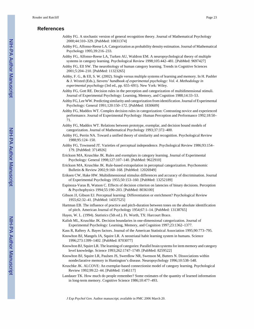
ReferencesAshby FG. A stochastic version of general recognition theory. Journal of Mathematical Psychology

2000;44:310–329. [PubMed: 10831374]Ashby FG, Alfonso-Reese LA. Categorization as probability density estimation. Journal of Mathematical

Psychology 1995;39:216–233.Ashby FG, Alfonso-Reese LA, Turken AU, Waldron EM. A neuropsychological theory of multiple

systems in category learning. Psychological Review 1998;105:442–481. [PubMed: 9697427]Ashby FG, Ell SW. The neurobiology of human category learning. Trends in Cognitive Sciences

2001;5:204–210. [PubMed: 11323265]Ashby, F. G., & Ell, S. W. (2002). Single versus multiple systems of learning and memory. In H. Pashler

& J. Wixted (Eds.), Stevens’ handbook of experimental psychology: Vol. 4. Methodology inexperimental psychology (3rd ed., pp. 655–691). New York: Wiley.

Ashby FG, Gott RE. Decision rules in the perception and categorization of multidimensional stimuli.Journal of Experimental Psychology: Learning, Memory, and Cognition 1988;14:33–53.

Ashby FG, Lee WW. Predicting similarity and categorization from identification. Journal of ExperimentalPsychology: General 1991;120:150–172. [PubMed: 1830609]

Ashby FG, Maddox WT. Complex decision rules in categorization: Contrasting novice and experiencedperformance. Journal of Experimental Psychology: Human Perception and Performance 1992;18:50–71.

Ashby FG, Maddox WT. Relations between prototype, exemplar, and decision bound models ofcategorization. Journal of Mathematical Psychology 1993;37:372–400.

Ashby FG, Perrin NA. Toward a unified theory of similarity and recognition. Psychological Review1988;95:124–150.

Ashby FG, Townsend JT. Varieties of perceptual independence. Psychological Review 1986;93:154–179. [PubMed: 3714926]

Erickson MA, Kruschke JK. Rules and exemplars in category learning. Journal of ExperimentalPsychology: General 1998;127:107–140. [PubMed: 9622910]

Erickson MA, Kruschke JK. Rule-based extrapolation in perceptual categorization. PsychonomicBulletin & Review 2002;9:160–168. [PubMed: 12026949]

Eriksen CW, Hake HW. Multidimensional stimulus differences and accuracy of discrimination. Journalof Experimental Psychology 1955;50:153–160. [PubMed: 13252189]

Espinoza-Varas B, Watson C. Effects of decision criterion on latencies of binary decisions. Perception& Psychophysics 1994;55:190–203. [PubMed: 8036100]

Gibson JJ, Gibson EJ. Perceptual learning: Differentiation or enrichment? Psychological Review1955;62:32–41. [PubMed: 14357525]

Hartman EB. The influence of practice and pitch-duration between tones on the absolute identificationof pitch. American Journal of Psychology 1954;67:1–14. [PubMed: 13138765]

Hayes, W. L. (1994). Statistics (5th ed.). Ft. Worth, TX: Harcourt Brace.Kalish ML, Kruschke JK. Decision boundaries in one-dimensional categorization. Journal of

Experimental Psychology: Learning, Memory, and Cognition 1997;23:1362–1377.Kass R, Raftery A. Bayes factors. Journal of the American Statistical Association 1995;90:773–795.Knowlton BJ, Mangels JA, Squire LR. A neostriatal habit learning system in humans. Science

1996;273:1399–1402. [PubMed: 8703077]Knowlton BJ, Squire LR. The learning of categories: Parallel brain systems for item memory and category

level knowledge. Science 1993;262:1747–1749. [PubMed: 8259522]Knowlton BJ, Squire LR, Paulsen JS, Swerdlow NR, Swenson M, Butters N. Dissociations within

nondeclarative memory in Huntington’s disease. Neuropsychology 1996;10:538–548.Kruschke JK. ALCOVE: An exemplar-based connectionist model of category learning. Psychological

Review 1992;99:22–44. [PubMed: 1546117]Landauer TK. How much do people remember? Some estimates of the quantity of learned information

in long-term memory. Cognitive Science 1986;10:477–493.

Rouder and Ratcliff Page 23

J Exp Psychol Gen. Author manuscript; available in PMC 2006 March 20.

NIH

-PA Author Manuscript

NIH

-PA Author Manuscript

NIH

-PA Author Manuscript

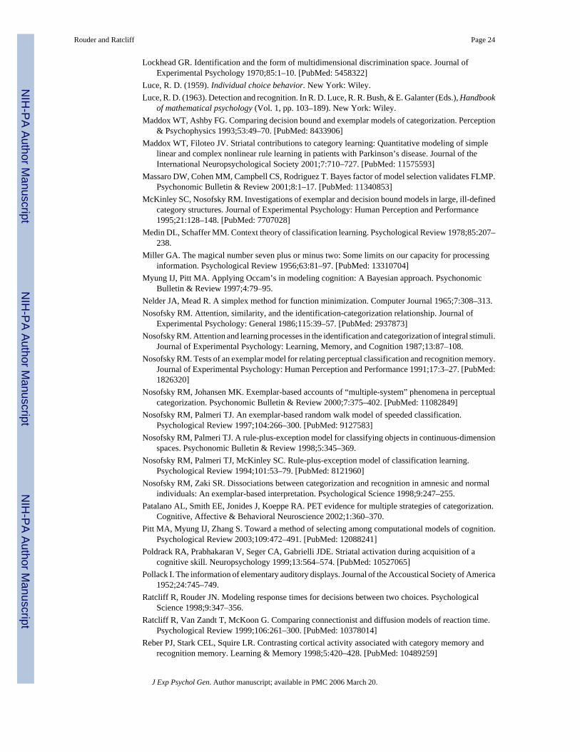
Lockhead GR. Identification and the form of multidimensional discrimination space. Journal ofExperimental Psychology 1970;85:1–10. [PubMed: 5458322]

Luce, R. D. (1959). Individual choice behavior. New York: Wiley.Luce, R. D. (1963). Detection and recognition. In R. D. Luce, R. R. Bush, & E. Galanter (Eds.), Handbook

of mathematical psychology (Vol. 1, pp. 103–189). New York: Wiley.Maddox WT, Ashby FG. Comparing decision bound and exemplar models of categorization. Perception

& Psychophysics 1993;53:49–70. [PubMed: 8433906]Maddox WT, Filoteo JV. Striatal contributions to category learning: Quantitative modeling of simple

linear and complex nonlinear rule learning in patients with Parkinson’s disease. Journal of theInternational Neuropsychological Society 2001;7:710–727. [PubMed: 11575593]

Massaro DW, Cohen MM, Campbell CS, Rodriguez T. Bayes factor of model selection validates FLMP.Psychonomic Bulletin & Review 2001;8:1–17. [PubMed: 11340853]

McKinley SC, Nosofsky RM. Investigations of exemplar and decision bound models in large, ill-definedcategory structures. Journal of Experimental Psychology: Human Perception and Performance1995;21:128–148. [PubMed: 7707028]

Medin DL, Schaffer MM. Context theory of classification learning. Psychological Review 1978;85:207–238.

Miller GA. The magical number seven plus or minus two: Some limits on our capacity for processinginformation. Psychological Review 1956;63:81–97. [PubMed: 13310704]

Myung IJ, Pitt MA. Applying Occam’s in modeling cognition: A Bayesian approach. PsychonomicBulletin & Review 1997;4:79–95.

Nelder JA, Mead R. A simplex method for function minimization. Computer Journal 1965;7:308–313.Nosofsky RM. Attention, similarity, and the identification-categorization relationship. Journal of

Experimental Psychology: General 1986;115:39–57. [PubMed: 2937873]Nosofsky RM. Attention and learning processes in the identification and categorization of integral stimuli.

Journal of Experimental Psychology: Learning, Memory, and Cognition 1987;13:87–108.Nosofsky RM. Tests of an exemplar model for relating perceptual classification and recognition memory.

Journal of Experimental Psychology: Human Perception and Performance 1991;17:3–27. [PubMed:1826320]

Nosofsky RM, Johansen MK. Exemplar-based accounts of “multiple-system” phenomena in perceptualcategorization. Psychonomic Bulletin & Review 2000;7:375–402. [PubMed: 11082849]

Nosofsky RM, Palmeri TJ. An exemplar-based random walk model of speeded classification.Psychological Review 1997;104:266–300. [PubMed: 9127583]

Nosofsky RM, Palmeri TJ. A rule-plus-exception model for classifying objects in continuous-dimensionspaces. Psychonomic Bulletin & Review 1998;5:345–369.

Nosofsky RM, Palmeri TJ, McKinley SC. Rule-plus-exception model of classification learning.Psychological Review 1994;101:53–79. [PubMed: 8121960]

Nosofsky RM, Zaki SR. Dissociations between categorization and recognition in amnesic and normalindividuals: An exemplar-based interpretation. Psychological Science 1998;9:247–255.

Patalano AL, Smith EE, Jonides J, Koeppe RA. PET evidence for multiple strategies of categorization.Cognitive, Affective & Behavioral Neuroscience 2002;1:360–370.

Pitt MA, Myung IJ, Zhang S. Toward a method of selecting among computational models of cognition.Psychological Review 2003;109:472–491. [PubMed: 12088241]

Poldrack RA, Prabhakaran V, Seger CA, Gabrielli JDE. Striatal activation during acquisition of acognitive skill. Neuropsychology 1999;13:564–574. [PubMed: 10527065]

Pollack I. The information of elementary auditory displays. Journal of the Accoustical Society of America1952;24:745–749.

Ratcliff R, Rouder JN. Modeling response times for decisions between two choices. PsychologicalScience 1998;9:347–356.

Ratcliff R, Van Zandt T, McKoon G. Comparing connectionist and diffusion models of reaction time.Psychological Review 1999;106:261–300. [PubMed: 10378014]

Reber PJ, Stark CEL, Squire LR. Contrasting cortical activity associated with category memory andrecognition memory. Learning & Memory 1998;5:420–428. [PubMed: 10489259]

Rouder and Ratcliff Page 24

J Exp Psychol Gen. Author manuscript; available in PMC 2006 March 20.

NIH

-PA Author Manuscript

NIH

-PA Author Manuscript

NIH

-PA Author Manuscript

Rouder JN. Absolute identification with simple and complex stimuli. Psychological Science2001;12:318–322. [PubMed: 11476099]

Rouder JN, Gomez P. Modeling serial position curves with temporal distinctiveness. Memory2001;9:301–311.

Rouder, J. N., Morey, R. D., Cowan, N., & Pfaltz, M. (in press). Learning in a unidimensional absoluteidentification task. Psychonomic Bulletin & Review.

Shepard RN. Stimulus and response generation: A stochastic model relating generalization to distancein a psychological space. Psychometrika 1957;22:325–345.

Shepard RN. Toward a universal law of generalization for psychological science. Science1987;237:1317–1323. [PubMed: 3629243]

Shiffrin RM, Nosofsky RM. Seven plus or minus two: A commentary on capacity limitations.Psychological Review 1994;101:357–361. [PubMed: 8022968]

Thomas RD. Learning correlations in categorization tasks using large, ill-defined categories. Journal ofExperimental Psychology: Learning, Memory, and Cognition 1998;24:119–143.

Trabasso, T., & Bower, G. H. (1968). Attention in learning: Theory and research. New York: Wiley.Waldron EM, Ashby FG. The effects of concurrent task interference on category learning: Evidence for

multiple category learning systems. Psychonomic Bulletin & Review 2001;8:168–176. [PubMed:11340863]

Wickelgren WA. Unidimensional strength theory and component analysis of noise in absolute andcomparative judgments. Journal of Mathematical Psychology 1968;5:102–122.

Zaki SR, Nosofsky RM. A single-system interpretation of dissociations between recognition andcategorization in a task involving object-like stimuli. Cognitive, Affective & BehavioralNeuroscience 2002;1:344–359.

Rouder and Ratcliff Page 25

J Exp Psychol Gen. Author manuscript; available in PMC 2006 March 20.

NIH

-PA Author Manuscript

NIH

-PA Author Manuscript

NIH

-PA Author Manuscript

Figure 1.A: Category structure and decision bound for Ratcliff and Rouder’s (1998) univariate design.B: Relative proportion of Category A exemplars for Ratcliff and Rouder’s design. C: Categorystructure and decision bound for Maddox and Ashby’s (1993) design. Categories werecomposed of bivariate normal distributions, which are represented as ellipses. D: Relativeproportion of Category A exemplars for Maddox and Ashby’s design. Lighter areas correspondto higher proportions. E and F: Category structure, decision bounds, and relative proportion ofCategory A exemplars for McKinley and Nosofsky’s (1995) design. Categories were composedof mixtures of bivariate normal distributions; each component is represented with an ellipse.Panel A is from “Modeling Response Times for Decisions Between Two Choices,” by R.Ratcliff and J. N. Rouder, 1998, Psychological Science, 9, p. 350. Copyright 1998 by BlackwellPublishing. Adapted with permission. Panel C is from “Comparing Decision Bound andExemplar Models of Categorization,” by W. T. Maddox and F. G. Ashby, 1993, Perception &Psychophysics, 53, p. 55. Copyright 1993 by the Psychonomic Society. Adapted withpermission. Panel E is from “Investigations of Exemplar and Decision Bound Models in Large,Ill-Defined Category Structures,” by S. C. McKinley and R. M. Nosofsky, 1995, Journal ofExperimental Psychology: Human Perception and Performance, 21, p. 135. Copyright 1995by the American Psychological Association. Adapted with permission of the author.

Rouder and Ratcliff Page 26

J Exp Psychol Gen. Author manuscript; available in PMC 2006 March 20.

NIH

-PA Author Manuscript

NIH

-PA Author Manuscript

NIH

-PA Author Manuscript

Figure 2.A: Category assignment probabilities as a function of luminance. B: Typical rule-basedpredictions. C: Typical exemplar-based predictions.

Rouder and Ratcliff Page 27

J Exp Psychol Gen. Author manuscript; available in PMC 2006 March 20.

NIH

-PA Author Manuscript

NIH

-PA Author Manuscript

NIH

-PA Author Manuscript

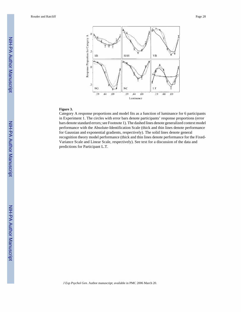
Figure 3.Category A response proportions and model fits as a function of luminance for 6 participantsin Experiment 1. The circles with error bars denote participants’ response proportions (errorbars denote standard errors; see Footnote 1). The dashed lines denote generalized context modelperformance with the Absolute-Identification Scale (thick and thin lines denote performancefor Gaussian and exponential gradients, respectively). The solid lines denote generalrecognition theory model performance (thick and thin lines denote performance for the Fixed-Variance Scale and Linear Scale, respectively). See text for a discussion of the data andpredictions for Participant L.T.

Rouder and Ratcliff Page 28

J Exp Psychol Gen. Author manuscript; available in PMC 2006 March 20.

NIH

-PA Author Manuscript

NIH

-PA Author Manuscript

NIH

-PA Author Manuscript

Figure 4.A general recognition theory model for absolute identification. The perceived luminance scaleis partitioned into regions corresponding to the eight different stimuli.’

Rouder and Ratcliff Page 29

J Exp Psychol Gen. Author manuscript; available in PMC 2006 March 20.

NIH

-PA Author Manuscript

NIH

-PA Author Manuscript

NIH

-PA Author Manuscript

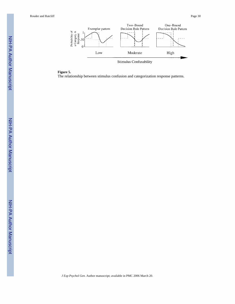
Figure 5.The relationship between stimulus confusion and categorization response patterns.

Rouder and Ratcliff Page 30

J Exp Psychol Gen. Author manuscript; available in PMC 2006 March 20.

NIH

-PA Author Manuscript

NIH

-PA Author Manuscript

NIH

-PA Author Manuscript

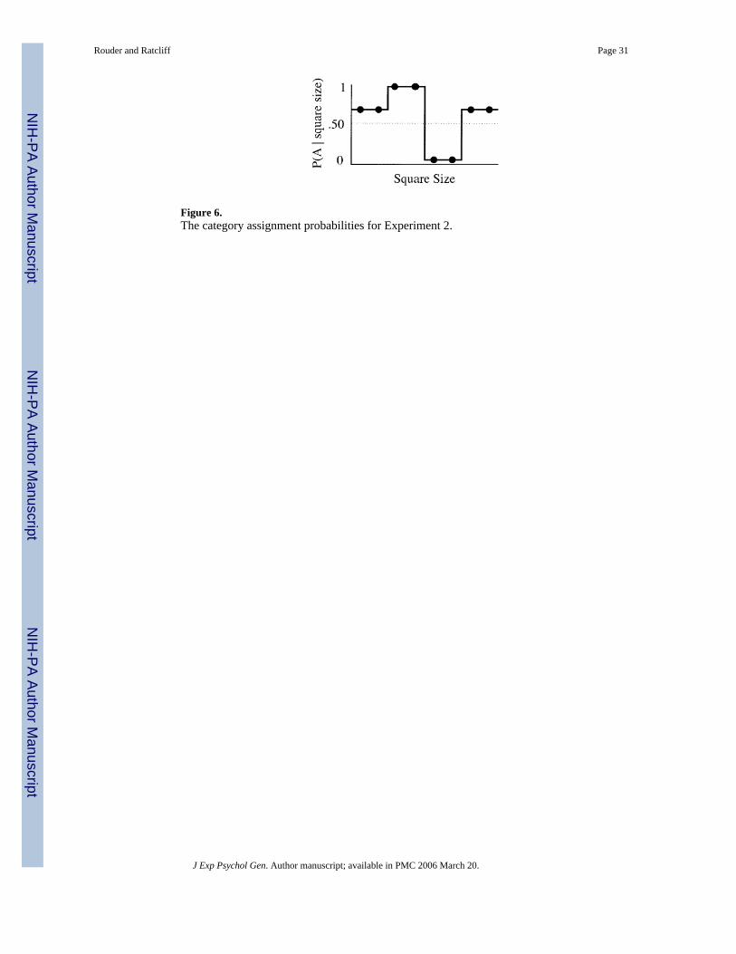
Figure 6.The category assignment probabilities for Experiment 2.

Rouder and Ratcliff Page 31

J Exp Psychol Gen. Author manuscript; available in PMC 2006 March 20.

NIH

-PA Author Manuscript

NIH

-PA Author Manuscript

NIH

-PA Author Manuscript

Figure 7.The types of response patterns observed in Experiment 2. Each panel shows responseproportions and model predictions for selected participants. Circles with error bars denoteresponse proportions and standard errors, respectively. The solid lines denote predictions froma general recognition theory model with the Linear Scale. The dashed lines denote predictionsfrom a generalized context model with the Gaussian similarity gradient and the Absolute-Identification Scale.

Rouder and Ratcliff Page 32

J Exp Psychol Gen. Author manuscript; available in PMC 2006 March 20.

NIH

-PA Author Manuscript

NIH

-PA Author Manuscript

NIH

-PA Author Manuscript

Figure 8.Cumulative distribution functions of the natural logarithm of chi-square fit statistics for square-size increment conditions of 5 and 15 in Experiment 2. The cumulative probability is obtainedby ordering participants’ chi-square fit statistics. The three thick lines denote generalrecognition theory (GRT) model fits; the four thin lines denote generalized context model(GCM) fits.

Rouder and Ratcliff Page 33

J Exp Psychol Gen. Author manuscript; available in PMC 2006 March 20.

NIH

-PA Author Manuscript

NIH

-PA Author Manuscript

NIH

-PA Author Manuscript

Figure 9.Category assignment probabilities for Experiment 3.

Rouder and Ratcliff Page 34

J Exp Psychol Gen. Author manuscript; available in PMC 2006 March 20.

NIH

-PA Author Manuscript

NIH

-PA Author Manuscript

NIH

-PA Author Manuscript

Figure 10.Category A response proportions and model fits as a function of square size for 6 participantsin Experiment 3. The circles with error bars denote participants’ response proportions (errorbars denote standard errors; see Footnote 1). The solid lines denote predictions from a generalrecognition theory model with the Linear Scale. The dashed lines denote predictions from ageneralized context model with the Gaussian similarity gradient and the Linear Scale.

Rouder and Ratcliff Page 35

J Exp Psychol Gen. Author manuscript; available in PMC 2006 March 20.

NIH

-PA Author Manuscript

NIH

-PA Author Manuscript

NIH

-PA Author Manuscript

Figure 11.Category assignment probabilities for Experiment 4.

Rouder and Ratcliff Page 36

J Exp Psychol Gen. Author manuscript; available in PMC 2006 March 20.

NIH

-PA Author Manuscript

NIH

-PA Author Manuscript

NIH

-PA Author Manuscript

Figure 12.Results from Experiment 4. Data are means over all participants. Error bars denote standarderrors and were calculated across participants.

Rouder and Ratcliff Page 37

J Exp Psychol Gen. Author manuscript; available in PMC 2006 March 20.

NIH

-PA Author Manuscript

NIH

-PA Author Manuscript

NIH

-PA Author Manuscript

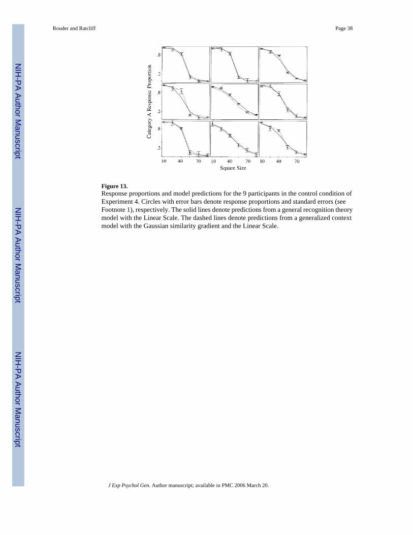
Figure 13.Response proportions and model predictions for the 9 participants in the control condition ofExperiment 4. Circles with error bars denote response proportions and standard errors (seeFootnote 1), respectively. The solid lines denote predictions from a general recognition theorymodel with the Linear Scale. The dashed lines denote predictions from a generalized contextmodel with the Gaussian similarity gradient and the Linear Scale.

Rouder and Ratcliff Page 38

J Exp Psychol Gen. Author manuscript; available in PMC 2006 March 20.

NIH

-PA Author Manuscript

NIH

-PA Author Manuscript

NIH

-PA Author Manuscript

Figure 14.Response proportions and model predictions for the 12 participants in the experimentalcondition of Experiment 4. Circles with error bars denote response proportions and standarderrors (see Footnote 1), respectively. Solid and dashed lines denote general recognition theory(GRT) and generalized context model (GCM) predictions, respectively. The solid lines denotepredictions from a GRT model with the Linear Scale. The dashed lines denote predictions froma GCM model with the Gaussian similarity gradient and the Linear Scale.

Rouder and Ratcliff Page 39

J Exp Psychol Gen. Author manuscript; available in PMC 2006 March 20.

NIH

-PA Author Manuscript

NIH

-PA Author Manuscript

NIH

-PA Author Manuscript

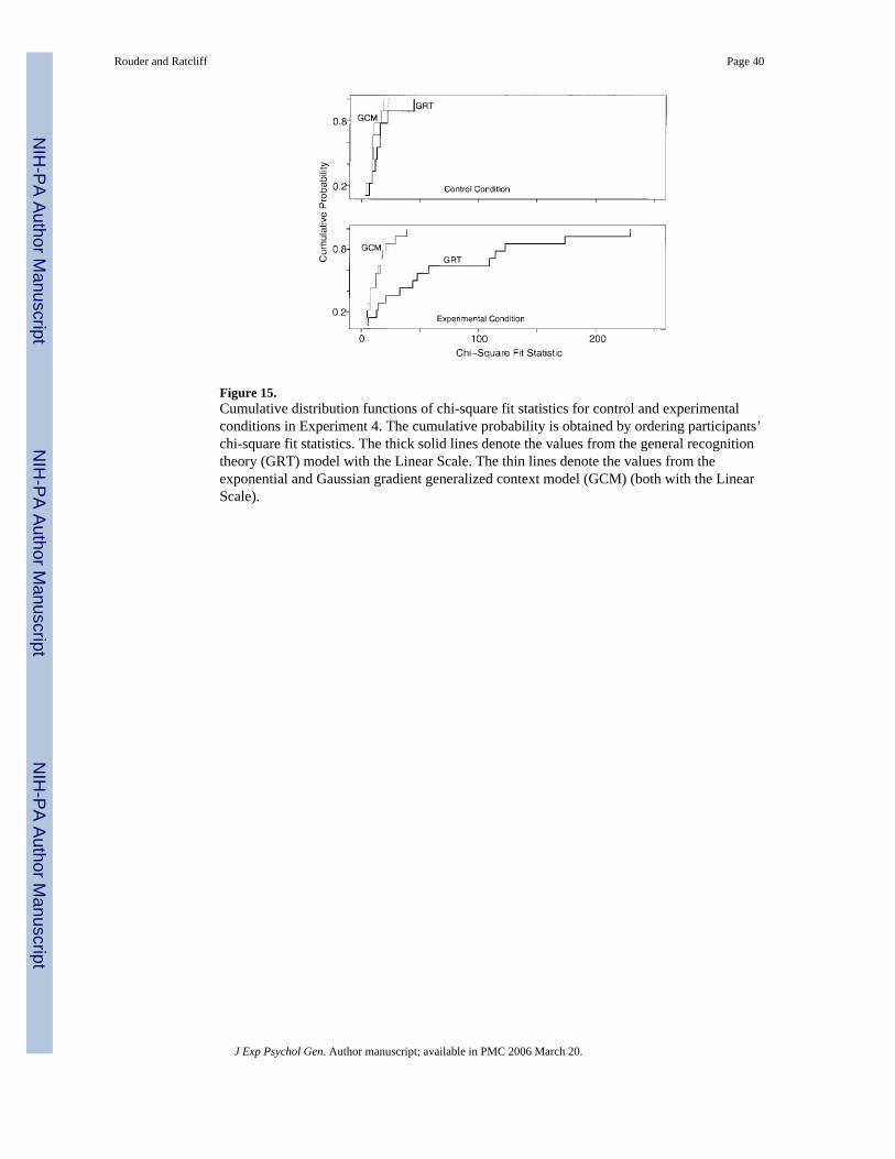
Figure 15.Cumulative distribution functions of chi-square fit statistics for control and experimentalconditions in Experiment 4. The cumulative probability is obtained by ordering participants’chi-square fit statistics. The thick solid lines denote the values from the general recognitiontheory (GRT) model with the Linear Scale. The thin lines denote the values from theexponential and Gaussian gradient generalized context model (GCM) (both with the LinearScale).

Rouder and Ratcliff Page 40

J Exp Psychol Gen. Author manuscript; available in PMC 2006 March 20.

NIH

-PA Author Manuscript

NIH

-PA Author Manuscript

NIH

-PA Author Manuscript

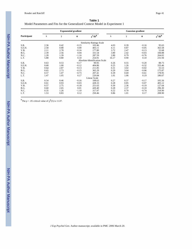
NIH

-PA Author Manuscript

NIH

-PA Author Manuscript

NIH

-PA Author Manuscript

Rouder and Ratcliff Page 41

Table 1Model Parameters and Fits for the Generalized Context Model in Experiment 1

Exponential gradient Gaussian gradient

Participant λ γ φ χ2 fita λ γ φ χ2 fita

Similarity-Ratings ScaleS.B. 2.36 0.42 −0.15 103.46 4.03 0.39 −0.16 95.63S.E.H. 2.58 0.88 0.00 403.11 4.11 0.87 −0.05 363.58V.B. 2.11 2.78 −0.16 177.80 3.72 2.47 −0.13 52.68B.G. 2.39 2.56 0.04 331.54 3.80 2.42 −0.03 184.88N.C. 1.28 1.39 −1.16 287.59 2.80 0.79 −0.76 264.02L.T. 5.88 0.80 0.10 254.91 16.17 0.90 0.10 231.94

Absolute-Identification ScaleS.B. 0.63 0.53 −0.17 99.95 0.26 0.55 −0.20 88.73S.E.H. 0.68 1.00 −0.12 404.86 0.25 1.26 −0.32 333.46V.B. 0.64 2.87 −0.13 211.85 0.31 3.02 −0.02 55.53B.G. 0.65 2.73 −0.15 365.29 0.29 3.04 −0.06 175.87N.C. 0.57 1.07 −0.73 207.41 0.39 0.69 −0.61 178.95L.T. 1.47 1.05 0.17 220.84 1.01 1.06 0.19 186.67

Linear ScaleS.B. 0.54 0.46 −0.16 108.63 0.27 0.37 −0.17 105.56S.E.H. 0.61 0.93 −0.03 428.33 0.28 0.85 −0.07 405.12V.B. 0.57 2.75 −0.18 251.63 0.30 2.36 −0.19 127.64B.G. 0.60 2.65 0.01 420.40 0.28 2.37 −0.10 296.30N.C. 0.35 1.26 −1.10 317.97 0.22 0.70 −0.74 318.90L.T. 1.53 0.83 0.12 250.46 0.86 1.01 0.17 208.90

aThe p < .05 critical value of χ2(5) is 11.07.

J Exp Psychol Gen. Author manuscript; available in PMC 2006 March 20.

NIH

-PA Author Manuscript

NIH

-PA Author Manuscript

NIH

-PA Author Manuscript

Rouder and Ratcliff Page 42

Table 2Model Parameters and Fits for the General Recognition Theory in Experiment 1

Participant Lower bound Upper bound σ0 Additional third bound χ2 fita

Luminance scaled by free-variance modelS.B. −2.34 2.54 2.53 43.1S.E.H. −1.72 2.71 1.48 42.9V.B. −0.68 4.33 1.82 265.7B.G. −0.57 3.96 1.15 73.5N.C. −0.76 1.71 1.28 66.2L.T. −0.16 3.25 1.19 −3.56 138.7b

Luminance scaled by fixed-variance modelS.B. −1.93 3.09 3.13 21.7S.E.H. −1.43 2.93 1.74 45.4V.B. −0.60 4.41 1.85 259.4B.G. −0.53 4.23 1.12 36.3N.C. −0.60 1.53 1.22 77.6L.T. −0.19 3.67 1.41 −3.40 97.9b

Linear ScaleS.B. −1.73 2.35 2.35 7.5S.E.H. −1.34 2.45 1.34 8.0V.B. −0.12 3.21 0.97 239.3B.G. −0.43 3.32 1.04 114.1N.C. −0.58 1.69 1.27 39.1L.T. 0.00 2.93 0.94 −2.89 7.0b

aThe p < .05 critical value of χ2(5) is 11.07.

bFits to L.T. were with additional third bound.

J Exp Psychol Gen. Author manuscript; available in PMC 2006 March 20.

NIH

-PA Author Manuscript

NIH

-PA Author Manuscript

NIH

-PA Author Manuscript

Rouder and Ratcliff Page 43

Table 3Effect of Increment Conditions in Experiment 2

Increment

Measure 5 7 10 15

MeansRight-tail increase .31 .45 .67 .65Left-tail decrease .01 .01 .03 .05

Mean ranksRight-tail increase 20.0 26.5 35.5 35.8Left-tail decrease 24.8 25.6 29.8 37.1

J Exp Psychol Gen. Author manuscript; available in PMC 2006 March 20.

NIH

-PA Author Manuscript

NIH

-PA Author Manuscript

NIH

-PA Author Manuscript

Rouder and Ratcliff Page 44

Table 4Chi-Square Goodness-of-Fit Values for Experiment 3

Participant

Model Gradient Scale 1 2 3 4 5 6

GCM Gaussian Similarity 3.3 8.5 5.7 12.0 0.8 1.5GCM Gaussian Linear/

Ordinal Position2.9 8.4 5.7 11.4 0.6 1.7

GCM Gaussian Linear/Square Size 13.0 21.1 3.4 33.9 18.1 5.7GCM Exponential Similarity 3.8 5.0 8.4 15.8 3.1 2.3GCM Exponential Linear/

Ordinal Position3.6 4.9 8.4 15.4 2.9 2.4

GCM Exponential Linear/Square Size 12.7 8.3 7.7 24.9 8.0 1.3GRT Linear/

Ordinal Position321.3 46.2 1.0 364.0 327.1 86.8

GRT Linear/Square Size 171.6 46.0 1.1 232.8 190.5 82.1

Note. GCM = generalized context model; GRT = general recognition theory.

J Exp Psychol Gen. Author manuscript; available in PMC 2006 March 20.