Comparative Study on Spatial Digital Mapping Methods of Soil ...

sustainability

Article

Comparative Study on Spatial Digital Mapping Methods ofSoil Nutrients Based on Different Geospatial Technologies

Li Gao 1 , Mingjing Huang 2, Wuping Zhang 3,*, Lei Qiao 1, Guofang Wang 1 and Xumeng Zhang 1

�����������������

Citation: Gao, L.; Huang, M.; Zhang,

W.; Qiao, L.; Wang, G.; Zhang, X.

Comparative Study on Spatial Digital

Mapping Methods of Soil Nutrients

Based on Different Geospatial

Technologies. Sustainability 2021, 13,

3270. https://doi.org/10.3390/

su13063270

Academic Editor: Clara Celauro

Received: 21 January 2021

Accepted: 12 March 2021

Published: 16 March 2021

Publisher’s Note: MDPI stays neutral

with regard to jurisdictional claims in

published maps and institutional affil-

iations.

Copyright: © 2021 by the authors.

Licensee MDPI, Basel, Switzerland.

This article is an open access article

distributed under the terms and

conditions of the Creative Commons

Attribution (CC BY) license (https://

creativecommons.org/licenses/by/

4.0/).

1 College of Resources and Environment, Shanxi Agricultural University, Taigu 030801, China;[email protected] (L.G.); [email protected] (L.Q.); [email protected] (G.W.);[email protected] (X.Z.)

2 Dryland Agriculture Research Center, Shanxi Agricultural University, Taiyuan 030031, China;[email protected]

3 College of Software, Shanxi Agricultural University, Taigu 030801, China* Correspondence: [email protected]

Abstract: Soil organic matter (SOM), total nitrogen (TN), available phosphorus (AP), and availablepotassium (AK) are important indicators of soil fertility when undertaking a quality evaluation.Obtaining a high-precision spatial distribution map of soil nutrients is of great significance for thedifferentiated management of nutrient resources and reducing non-point source pollution. How-ever, the spatial heterogeneity of soil nutrients lead to uncertainty in the modeling process. To deter-mine the best interpolation method, terrain, climate, and vegetation factors were used as auxiliaryvariables to participate in the investigation of soil nutrient spatial modeling in the present study. Weused the mean error (ME), mean absolute error (MAE), root mean square error (RMSE), and accuracy(Acc) of a dataset to comprehensively compare the performance of four different geospatial tech-niques: ordinary kriging (OK), regression kriging (RK), geographically weighted regression kriging(GWRK), and multiscale geographically weighted regression kriging (MGWRK). The results showedthat the hybrid methods (RK, GWRK, and MGWRK) could improve the prediction accuracy to acertain extent when the residuals were spatially correlated; however, this improvement was notsignificant. The new MGWRK model has certain advantages in reducing the overall residual level,but it failed to achieve the desired accuracy. Considering the cost of modeling, the OK method stillprovides an interpolation method with a relatively simple analysis process and relatively reliableresults. Therefore, it may be more beneficial to design soil sampling rationally and obtain higher-quality auxiliary variable data than to seek complex statistical methods to improve spatial predictionaccuracy. This research provides a reference for the spatial mapping of soil nutrients at the farmlandscale.

Keywords: soil nutrients; spatial non-stationarity; multiscale; MGWRK; soil digital mapping

1. Introduction

Soil nutrient indicators are key indicators for the evaluation of soil quality. Study-ing the spatial distribution of soil nutrients is the basis for understanding regional soilquality conditions, adjusting management measures and various material inputs, and ob-taining maximum benefits [1–3]. However, due to the combined effect of structure andrandomness [4,5], soil nutrients have a high degree of spatial heterogeneity and depen-dence [6]. Therefore, it is necessary but difficult to obtain more accurate spatial distributioninformation of soil nutrients in different regions.

In the past few decades, scholars have developed and applied many spatial inter-polation methods, including deterministic interpolation methods (e.g., inverse distanceweighted (IDW), radial basis function (RBF), global polynomial interpolation, and localpolynomial interpolation), geostatistical methods (e.g., ordinary kriging (OK), simplekriging, and CoKriging (COK)), and hybrid techniques (e.g., regression kriging (RK) and

Sustainability 2021, 13, 3270. https://doi.org/10.3390/su13063270 https://www.mdpi.com/journal/sustainability

Sustainability 2021, 13, 3270 2 of 19

geographically weighted regression kriging (GWRK)) [7]. Among these methods, the OKmethod is the most widely used geostatistical method. Through intensive field sampling,OK makes full use of the data information of the sample point, and can provide an estima-tion error for the interpolation results [8]. However, OK would consume large amountsof labor, material, and financial resources [9]. The sampling density and method have aconsiderable influence on the interpolation accuracy of OK [10]. Moreover, this methoddoes not incorporate environmental factors into the model, which are closely related tosoil nutrients. These limitations lead to the simulation of the spatial distribution of soilproperties in complex landscapes being greatly restricted [11,12].

With the rapid development of geographic information technology and remote sensingtechnology, other environmental factors that have the advantages of high accuracy andeasy access have gradually been incorporated into spatial modeling analyses. Many studieshave shown that methods that use environmental covariates (e.g., RK) usually producemore accurate simulations than OK. Watt and Palmer [13] used RK to draw a surface mapof New Zealand’s carbon/nitrogen ratio. Bangroo et al. [14] used RK to study the influenceof topographic factors on the spatial distribution of soil organic carbon (SOC) and totalsoil nitrogen (TSN); the authors found that the RK method was significantly better thanthe OK model in predicting SOC and TSN in the case of residuals with a moderate degreeof spatial autocorrelation. Mondal et al. [15] selected eight variables to predict SOC; theRK method also provided satisfactory results from the accuracy point of view due to theintroduction of additional auxiliary information. The RK method combines the trend itemand kriging residual item generated by global regression fitting [16,17]. Thus, it has theadvantages of easy implementation, detailed results, and high prediction accuracy [18].

However, the relationships between soil nutrients and environmental covariatesare always non-stationary over space, but the RK method assumes that the relationshipbetween soil properties and environmental covariates is constant globally [12,19]. As aresult, RK cannot capture the local characteristics of the spatial variation of soil nutrients,and the improvement of interpolation accuracy is again restricted. To solve this problem,the local model GWRK has been applied. As a combination of geographically weightedregression (GWR) and kriging, this method embeds the spatial position into the regressionparameters through the idea of local weighted least squares [20,21]. It not only considersthe non-stationarity of the spatial parameters and the local relationship between the targetvariable and the explanatory variable, but also the spatial autocorrelation of the regressionresiduals [22]. The GWRK method provides good prediction results in most cases [23–25].

However, GWR also has certain limitations. The method uses a single bandwidthfor all variables, ignoring the different scales of the relationship between the independentvariable and the dependent variable. This may cause a lot of noise and bias in the regressioncoefficient, which may lead to unstable regression coefficients [26]. Nevertheless, scale isan important term in geographic research [27,28], and spatial phenomenon are inherentlyaffected by scale effects [29]. Therefore, the change in scale has a considerable impacton the model performance [30,31]. Murakami et al. [32] also emphasized the importanceof scale in local regression modeling. The first model to consider multi-scale effects wasthe hybrid GWR model. The regression coefficients of some parameters in this model areglobally fixed, while the remaining parameters are spatially variable [33–36]. However, thehybrid GWR is limited; it can only distinguish the scale influence of different variablesinto global and local scales, but the local coefficients of the variables still change within thesame scale [37]. Fotheringham et al. [38] proposed the multi-scale geographic weightedregression (MGWR) method in 2017 to allow multi-scale modeling, which allows the modelto run at different spatial scales by introducing a specific bandwidth for each variable.As an extension of MGWR, MGWRK [39] is similar to other hybrid methods. It not onlyretains the characteristics of MGWR, but also accounts for the relevance of the regressionresiduals; thus, it appears to be a promising method.

In summary, scholars have carried out a lot of research on the digital mapping of soilnutrients. Although the emergence of different methods is necessary, the portability of

Sustainability 2021, 13, 3270 3 of 19

these methods is generally poor. The selected explanatory variables differ between researchareas and for various scales, the best interpolation method may also differ between targetvariables. At the same time, as an emerging model, few studies have reported on theapplication of MGWRK at the farmland scale. Therefore, the main aims of the presentstudy are to select environmental factors such as, vegetation, terrain, and climate factors formodeling, and to compare the performance of different geospatial technologies (OK, RK,GWRK, and MGWRK) in soil nutrient mapping.

2. Materials and Methods2.1. Study Area

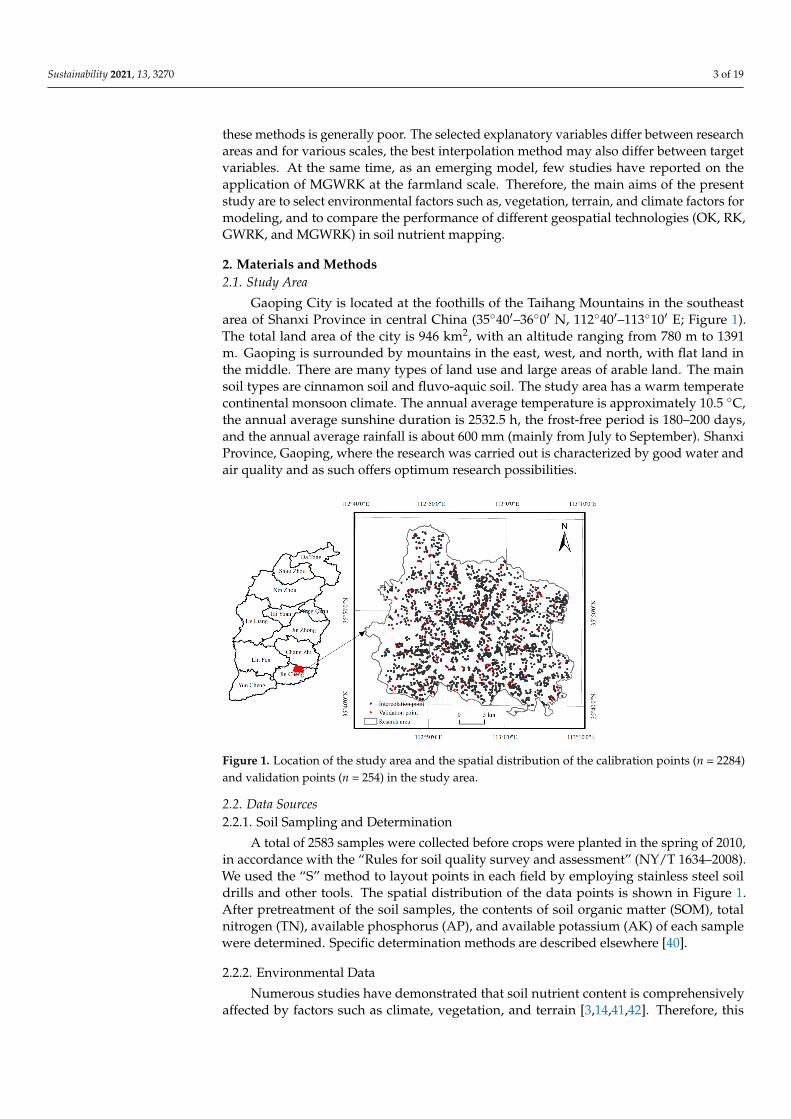
Gaoping City is located at the foothills of the Taihang Mountains in the southeastarea of Shanxi Province in central China (35◦40′–36◦0′ N, 112◦40′–113◦10′ E; Figure 1).The total land area of the city is 946 km2, with an altitude ranging from 780 m to 1391m. Gaoping is surrounded by mountains in the east, west, and north, with flat land inthe middle. There are many types of land use and large areas of arable land. The mainsoil types are cinnamon soil and fluvo-aquic soil. The study area has a warm temperatecontinental monsoon climate. The annual average temperature is approximately 10.5 ◦C,the annual average sunshine duration is 2532.5 h, the frost-free period is 180–200 days,and the annual average rainfall is about 600 mm (mainly from July to September). ShanxiProvince, Gaoping, where the research was carried out is characterized by good water andair quality and as such offers optimum research possibilities.

Figure 1. Location of the study area and the spatial distribution of the calibration points (n = 2284)and validation points (n = 254) in the study area.

2.2. Data Sources2.2.1. Soil Sampling and Determination

A total of 2583 samples were collected before crops were planted in the spring of 2010,in accordance with the “Rules for soil quality survey and assessment” (NY/T 1634–2008).We used the “S” method to layout points in each field by employing stainless steel soildrills and other tools. The spatial distribution of the data points is shown in Figure 1.After pretreatment of the soil samples, the contents of soil organic matter (SOM), totalnitrogen (TN), available phosphorus (AP), and available potassium (AK) of each samplewere determined. Specific determination methods are described elsewhere [40].

2.2.2. Environmental Data

Numerous studies have demonstrated that soil nutrient content is comprehensivelyaffected by factors such as climate, vegetation, and terrain [3,14,41,42]. Therefore, this

Sustainability 2021, 13, 3270 4 of 19

paper selected these factors as auxiliary variables to participate in the investigation of soilnutrient spatial modeling.

The climate factors included mean annual precipitation (MAP) and mean annualtemperature (MAT), which were obtained from National Meteorological Information Cen-ter [43]. We downloaded the precipitation and temperature data of local meteorologicalstations from 1980 to 2010. By calculating the average multi-year precipitation and averagemulti-year temperature, and by performing kriging interpolation, meteorological data ateach soil sampling point in Gaoping City were extracted.

The topographic factors were derived from the DEM (30 m spatial resolution) obtainedfrom Geospatial Data Cloud [44]. Based on the DEM data, we obtained various compositeterrain factor indicators in the SAGA-GIS software.

The remote-sensing data include the NDVI and vegetation coverage (VC), which werealso derived from Geospatial Data Cloud [44]. We downloaded Landsat 8 remote sensingimages that were consistent with the sampling time. After preprocessing the image, weused the band calculator to calculate the NDVI and VC to reflect the growth status offarmland vegetation in that year. The data of various environmental covariates are shownin Table 1.

Table 1. List of environmental covariate data.

Data Type Index

Terrain data

ElevationSlope

AspectPlane curvature, PC

Topographic relief, TRSurface roughness, SR

Topographic wetness index, TWI

Meteorological data Mean average precipitation, MAPMean average temperature, MAT

Remote sensing dataNormalized differential vegetation index,

NDVIVegetation coverage, VC

2.3. Geospatial Techniques2.3.1. Ordinary Kriging (OK)

The OK model is based on spatial autocorrelation and second-order stationary as-sumptions. It uses the semivariogram theory as a tool to analyze its spatial structure,and realizes the optimal unbiased linear estimation of the unknown area based on theexisting sampling point data in a limited area [11]. The semivariance function equation isdescribed as Equation (1).

γ(h) =1

2N(h)

N(h)

∑i=1

[Z(xi)− Z(xi + h)]2 (1)

where γ(h) is the semivariogram value; h is the lag; N(h) is the total number of point pairswith an interval of h; Z(xi) and Z(xi + h) are the measured values of regionalized variablesat positions xi and xi + h, respectively.

2.3.2. Regression Kriging (RK)

Regression kriging combines multiple linear regression (MLR) and kriging interpo-lation. The steps for establishing this method are as follows: a stepwise MLR analysis isperformed between the target variable and its highly correlated auxiliary variables to obtainthe trend item and residual item, which represent certainty and randomness, respectively.Then, OK is applied to interpolate the residual item of the regression model before finally

Sustainability 2021, 13, 3270 5 of 19

summing them up [16,18]. The fundamental equation of the RK model is described asEquation (2):

yRK(xi) = yMLR(xi) + yOK(xi) (2)

where yRK(xi) denotes the predicted value of the RK model at the point xi; yMLR(xi) is thetrend value of MLR at point xi; yOK(xi) is the residual item estimated by the OK method atthe point xi.

2.3.3. Geographically Weighted Regression Kriging (GWRK)

As a hybrid method, the modeling process of GWRK [25] is similar to that of RK,with the exception of the fact that the global fitting in RK is replaced with the local fittingin GWR. The GWR approach is used to deal with spatial non-stationarity by introducing aspatial location into regression coefficients [21].

Assuming that there is a total of n observation points, the location of each observationpoint is (ui, vi), and there is a total of m independent variables involved in modeling.The expression of the GWR model is shown in Equation (3):

yi =n

∑i=0

m

∑j=0

β j(ui, vi)xij + εi (3)

where xij is the jth independent variable at the observation point; βi(ui, vi) is the regressioncoefficient of the jth independent variable at the position (ui, vi); εi is the random errorterm; yi is dependent variable.

Two types of spatial weight function methods, the Gaussian function and Bi-squarefunction, are usually used to determine the spatial weight in GWR analysis. Differenttypes of kernel functions can be used during operation, including fixed kernel functionsand adaptive kernel functions. Research has shown that an adaptive kernel is arguablymore favorable when dealing with non-uniform spatial distributions [21,24]. Because thesampling points are not uniformly distributed, this study selects an adaptive Gaussiankernel function for modeling. In addition, geographic weighted regression analysis is verysensitive to the bandwidth selection of a specific weight function [45]. This study uses thecorrected Akaike information criterion (AICc) to determine the model bandwidth, wherethe principle is to minimize the AICc. This approach helps to evaluate whether the GWRmodel simulates the data better than the MLR model.

2.3.4. Multiscale Geographically Weighted Regression Kriging (MGWRK)

As mentioned, MGWRK [39] is a combination of MGWR and kriging interpolation.The MGWR model can be expressed as Equation (4):

yi =n

∑i=0

m

∑j=0

βbwj(ui, vi)xij + εi (4)

where βbwj is the regression coefficient corrected by the effective bandwidth of the jthindependent variable. In our study, the kernel functions and kernel types of MGWR andGWR models are consistent.

The MGWR model accounts for the spatial scale effect of the influence of different inde-pendent variables on the dependent variable, and provides different independent variableswith different bandwidths. This is the main difference between the MGWR model and theGWR model. All independent variables in the GWR model share a bandwidth, which can beregarded as a weighted average of different levels of spatial heterogeneity [38,46].

2.4. Model Validation and Evaluation

Ninety percent of sampling points (2284) were randomly selected from the originaldata as the prediction set to build the model, and the remaining 10% samples (254) wereused as the verification set to test the model’s prediction accuracy. We evaluated the

Sustainability 2021, 13, 3270 6 of 19

performance of different models by calculating the mean error (ME), mean absolute error(MAE), root mean square error (RMSE), and prediction accuracy (Acc) of the validationset [33,47]. These four indices can be written as Equations (5)–(8):

ME =1n

n

∑i=1

[Z(xi)− Z(xi)

](5)

MAE =1n

n

∑i=1

[∣∣Z(xi)− Z(xi)∣∣] (6)

RMSE =

√1n

n

∑i=1

[Z(xi)− Z(xi)

]2 (7)

Acc =

[1− 1

n

n

∑i=1

∣∣∣∣ Z(xi)− Z(xi)

Z(xi)

∣∣∣∣]

(8)

where Z(xi) is the predicted value at position xi; Z(xi) is the measured value at position xi;n is the number of samples.

In general, ME, MAE, and RMSE values closer to zero and a higher Acc give a betterprediction.

3. Results3.1. Descriptive Statistics

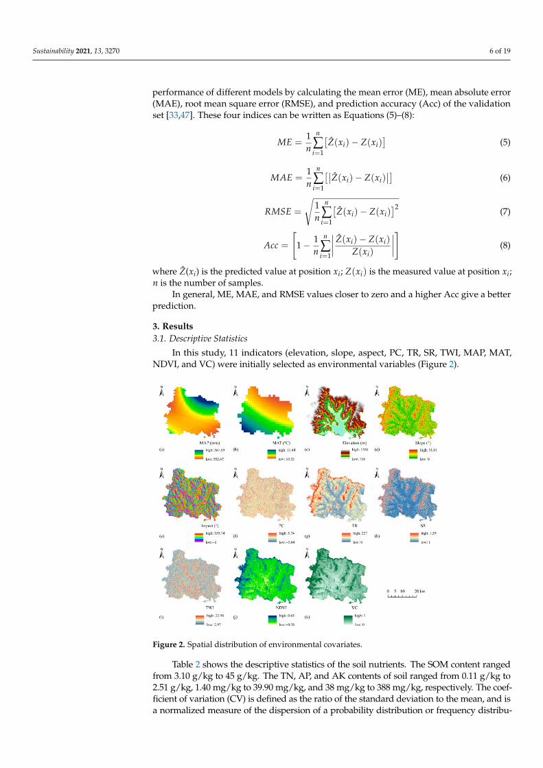
In this study, 11 indicators (elevation, slope, aspect, PC, TR, SR, TWI, MAP, MAT,NDVI, and VC) were initially selected as environmental variables (Figure 2).

Figure 2. Spatial distribution of environmental covariates.

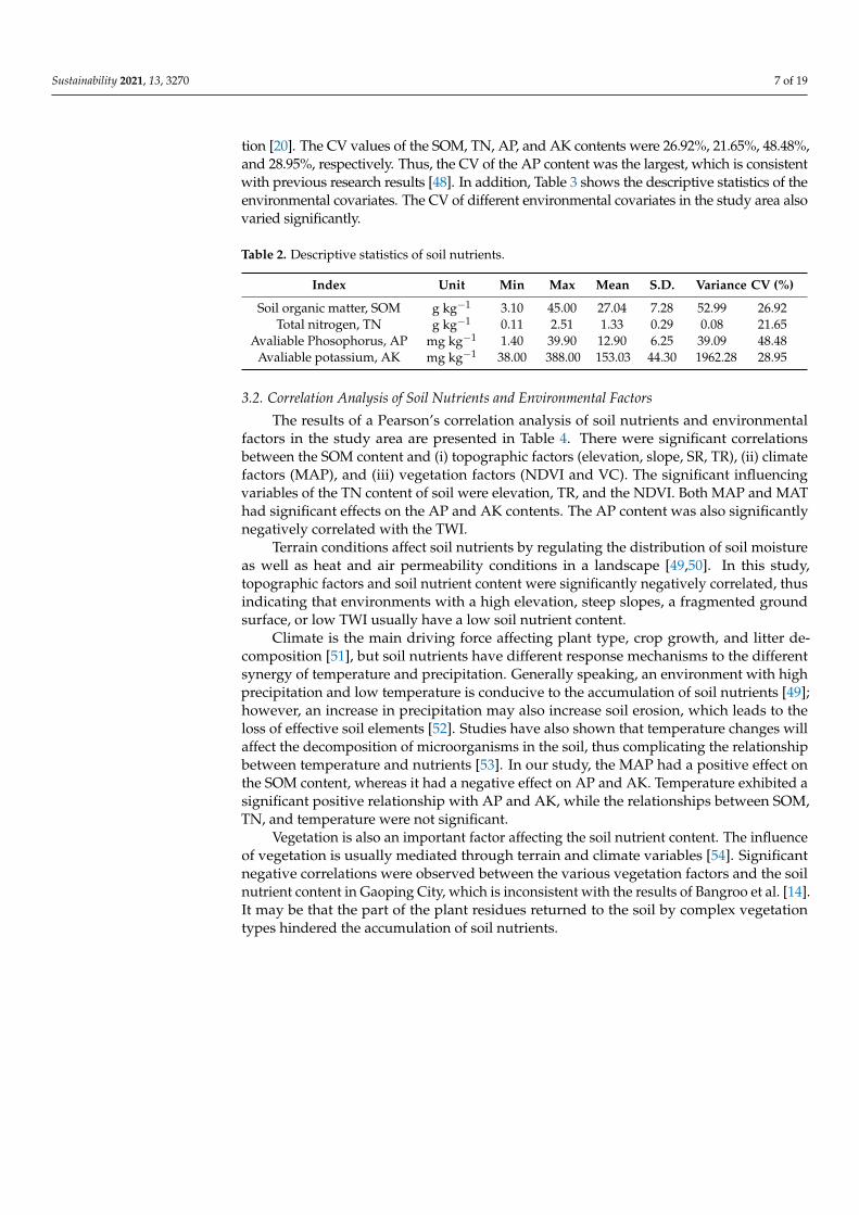
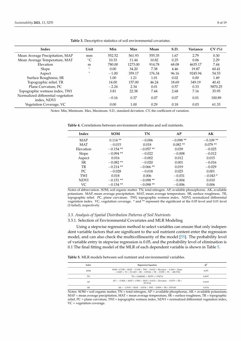
Table 2 shows the descriptive statistics of the soil nutrients. The SOM content rangedfrom 3.10 g/kg to 45 g/kg. The TN, AP, and AK contents of soil ranged from 0.11 g/kg to2.51 g/kg, 1.40 mg/kg to 39.90 mg/kg, and 38 mg/kg to 388 mg/kg, respectively. The coef-ficient of variation (CV) is defined as the ratio of the standard deviation to the mean, and isa normalized measure of the dispersion of a probability distribution or frequency distribu-

Sustainability 2021, 13, 3270 7 of 19

tion [20]. The CV values of the SOM, TN, AP, and AK contents were 26.92%, 21.65%, 48.48%,and 28.95%, respectively. Thus, the CV of the AP content was the largest, which is consistentwith previous research results [48]. In addition, Table 3 shows the descriptive statistics of theenvironmental covariates. The CV of different environmental covariates in the study area alsovaried significantly.

Table 2. Descriptive statistics of soil nutrients.

Index Unit Min Max Mean S.D. Variance CV (%)

Soil organic matter, SOM g kg−1 3.10 45.00 27.04 7.28 52.99 26.92Total nitrogen, TN g kg−1 0.11 2.51 1.33 0.29 0.08 21.65

Avaliable Phosophorus, AP mg kg−1 1.40 39.90 12.90 6.25 39.09 48.48Avaliable potassium, AK mg kg−1 38.00 388.00 153.03 44.30 1962.28 28.95

3.2. Correlation Analysis of Soil Nutrients and Environmental Factors

The results of a Pearson’s correlation analysis of soil nutrients and environmentalfactors in the study area are presented in Table 4. There were significant correlationsbetween the SOM content and (i) topographic factors (elevation, slope, SR, TR), (ii) climatefactors (MAP), and (iii) vegetation factors (NDVI and VC). The significant influencingvariables of the TN content of soil were elevation, TR, and the NDVI. Both MAP and MAThad significant effects on the AP and AK contents. The AP content was also significantlynegatively correlated with the TWI.

Terrain conditions affect soil nutrients by regulating the distribution of soil moistureas well as heat and air permeability conditions in a landscape [49,50]. In this study,topographic factors and soil nutrient content were significantly negatively correlated, thusindicating that environments with a high elevation, steep slopes, a fragmented groundsurface, or low TWI usually have a low soil nutrient content.

Climate is the main driving force affecting plant type, crop growth, and litter de-composition [51], but soil nutrients have different response mechanisms to the differentsynergy of temperature and precipitation. Generally speaking, an environment with highprecipitation and low temperature is conducive to the accumulation of soil nutrients [49];however, an increase in precipitation may also increase soil erosion, which leads to theloss of effective soil elements [52]. Studies have also shown that temperature changes willaffect the decomposition of microorganisms in the soil, thus complicating the relationshipbetween temperature and nutrients [53]. In our study, the MAP had a positive effect onthe SOM content, whereas it had a negative effect on AP and AK. Temperature exhibited asignificant positive relationship with AP and AK, while the relationships between SOM,TN, and temperature were not significant.

Vegetation is also an important factor affecting the soil nutrient content. The influenceof vegetation is usually mediated through terrain and climate variables [54]. Significantnegative correlations were observed between the various vegetation factors and the soilnutrient content in Gaoping City, which is inconsistent with the results of Bangroo et al. [14].It may be that the part of the plant residues returned to the soil by complex vegetationtypes hindered the accumulation of soil nutrients.

Sustainability 2021, 13, 3270 8 of 19

Table 3. Descriptive statistics of soil environmental covariates.

Index Unit Min Max Mean S.D. Variance CV (%)

Mean Average Precipitation, MAP mm 552.52 561.93 555.35 1.67 2.79 0.30Mean Average Temperature, MAT ◦C 10.33 11.44 10.82 0.25 0.06 2.29

Elevation m 780.00 1273.00 914.78 68.08 4635.17 7.44Slope ◦ 0.00 34.20 7.38 4.46 19.87 60.41

Aspect ◦ −1.00 359.17 176.34 96.16 9245.94 54.53Surface Roughness, SR 1.00 1.21 1.01 0.02 0.00 1.49Topographic relief, TR 14.00 157.00 46.24 18.69 349.19 40.41Plane Curvature, PC −2.24 2.34 0.01 0.57 0.33 5870.25

Topographic wetness index, TWI 3.81 22.38 7.44 2.68 7.16 35.95Normalized differential vegetation

index, NDVI −0.16 0.37 0.07 0.07 0.01 100.89

Vegetation Coverage, VC 0.00 1.00 0.29 0.18 0.03 61.33

Notes: Min, Minimum. Max, Maximum. S.D., standard deviation. CV, the coefficient of variation.

Table 4. Correlations between environment attributes and soil nutrients.

Index SOM TN AP AK

MAP 0.114 ** −0.006 −0.098 ** −0.109 **MAT −0.015 0.018 0.082 ** 0.079 **

Elevation −0.154 ** −0.057 ** 0.039 −0.025Slope −0.094 ** −0.022 −0.008 −0.012

Aspect 0.016 −0.002 0.012 0.015SR −0.082 ** −0.020 0.001 −0.016TR −0.214 ** −0.066 ** 0.019 −0.029PC −0.028 −0.018 0.025 0.001

TWI 0.018 0.006 −0.031 −0.043 *NDVI −0.151 ** −0.098 ** −0.004 0.010

VC −0.154 ** −0.098 ** −0.006 0.006Notes of abbreviation. SOM, soil organic matter. TN, total nitrogen. AP, available phosophorus. AK, availablepotassium. MAP, mean average precipitation. MAT, mean average temperature. SR, surface roughness. TR,topographic relief. PC, plane curvature. TWI, topographic wetness index. NDVI, normalized differentialvegetation index. VC, vegetation coverage. * and ** represent the significant at the 0.05 level and 0.01 level(2-tailed), respectively.

3.3. Analysis of Spatial Distribution Patterns of Soil Nutrients3.3.1. Selection of Environmental Covariates and MLR Modeling

Using a stepwise regression method to select variables can ensure that only indepen-dent variable factors that are significant to the soil nutrient content enter the regressionmodel, and can also check the multicollinearity of the model [55]. The probability levelof variable entry in stepwise regression is 0.05, and the probability level of elimination is0.1 The final fitting model of the MLR of each dependent variable is shown in Table 5.

Table 5. MLR models between soil nutrient and environmental variables.

Index Regression Equation R2

SOM SOM = 0.7188 ×MAP − 0.1338 × TWI − 0.0123 × Elevation − 0.1669 × Slope− 2.5425 × VC + 52.1433 × SR − 0.05106 × TR − 0.5255 × PC − 408.3766 0.075

TN TN = 0.4060069 × NDVI + 1.354716 0.0097

AP AP = −0.3824 ×MAP + 1.5562 ×MAT + 0.0123 × Elevation − 0.0170 × TR +197.9734 0.0193

AK AK = −2.9193 ×MAP − 0.8736 × TWI − 0.0909 × TR + 1785.001 0.0154

Notes: SOM = soil organic matter, TN = total nitrogen, AP = available phosphorus, AK = available potassium;MAP = mean average precipitation, MAT = mean average temperature, SR = surface roughness, TR = topographicrelief, PC = plane curvature, TWI = topographic wetness index, NDVI = normalized differential vegetation index,VC = vegetation coverage.

Sustainability 2021, 13, 3270 9 of 19

To further explore the influence of environmental covariates on the soil nutrientcontent in the study area at different locations, and to compare the differences in spatialmapping of different methods, the factors of the MLR model were also applied for GWRand MGWR modeling.

3.3.2. Spatial Variability Characteristics of Soil Nutrients and Residuals of MLR, GWR, andMGWR Models

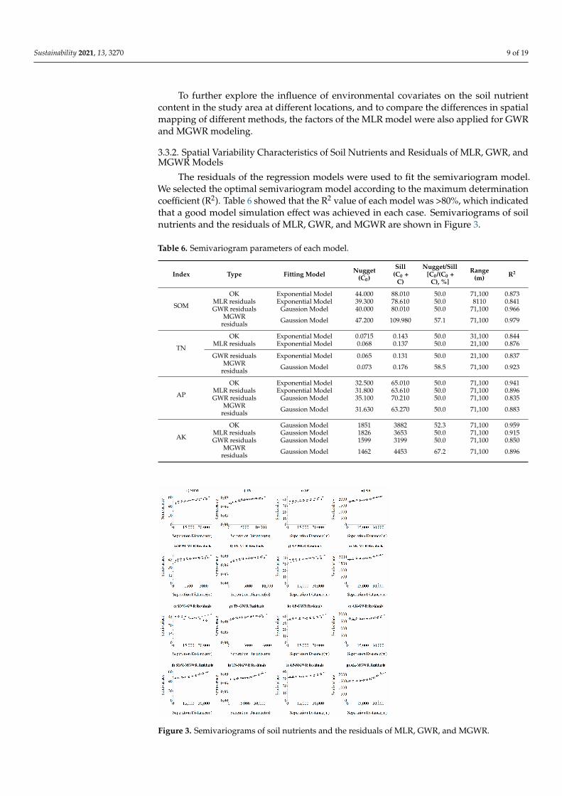
The residuals of the regression models were used to fit the semivariogram model.We selected the optimal semivariogram model according to the maximum determinationcoefficient (R2). Table 6 showed that the R2 value of each model was >80%, which indicatedthat a good model simulation effect was achieved in each case. Semivariograms of soilnutrients and the residuals of MLR, GWR, and MGWR are shown in Figure 3.

Table 6. Semivariogram parameters of each model.

Index Type Fitting Model Nugget(C0)

Sill(C0 +

C)

Nugget/Sill[C0/(C0 +

C), %]

Range(m) R2

SOM

OK Exponential Model 44.000 88.010 50.0 71,100 0.873MLR residuals Exponential Model 39.300 78.610 50.0 8110 0.841GWR residuals Gaussion Model 40.000 80.010 50.0 71,100 0.966

MGWRresiduals Gaussion Model 47.200 109.980 57.1 71,100 0.979

TN

OK Exponential Model 0.0715 0.143 50.0 31,100 0.844MLR residuals Exponential Model 0.068 0.137 50.0 21,100 0.876

GWR residuals Exponential Model 0.065 0.131 50.0 21,100 0.837MGWR

residuals Gaussion Model 0.073 0.176 58.5 71,100 0.923

AP

OK Exponential Model 32.500 65.010 50.0 71,100 0.941MLR residuals Exponential Model 31.800 63.610 50.0 71,100 0.896GWR residuals Gaussion Model 35.100 70.210 50.0 71,100 0.835

MGWRresiduals Gaussion Model 31.630 63.270 50.0 71,100 0.883

AK

OK Gaussion Model 1851 3882 52.3 71,100 0.959MLR residuals Gaussion Model 1826 3653 50.0 71,100 0.915GWR residuals Gaussion Model 1599 3199 50.0 71,100 0.850

MGWRresiduals Gaussion Model 1462 4453 67.2 71,100 0.896

Figure 3. Semivariograms of soil nutrients and the residuals of MLR, GWR, and MGWR.

Sustainability 2021, 13, 3270 10 of 19

The spatial autocorrelation for SOM in the various models ranged from 8110 m to71,100 m. The nugget values were 44 (OK), 39.3 (MLR residuals), 40 (GWR residuals),and 47.2 (MGWR residuals). The spatial autocorrelation for TN ranged up to 31,100m, and the spatial ranges of the residuals for MLR, GWR, and MGWR were 21,100 m,21,100 m, and 71,100 m, respectively. The nugget values were 0.0715 (OK), 0.068 (MLRresiduals), 0.065 (GWR residuals), and 0.073 (MGWR residuals). The spatial autocorrelationfor the AP in each model ranged up to 71,100 m. The nugget values were 32.5 (OK),31.8 (MLR residuals), 35.1 (GWR residuals), and 31.63 (MGWR residuals). The spatialautocorrelation for AK in each model also ranged up to 71,100 m. The nugget values were1851 (OK), 1826 (MLR residuals), 1599 (GWR residuals), and 1462 (MGWR residuals).

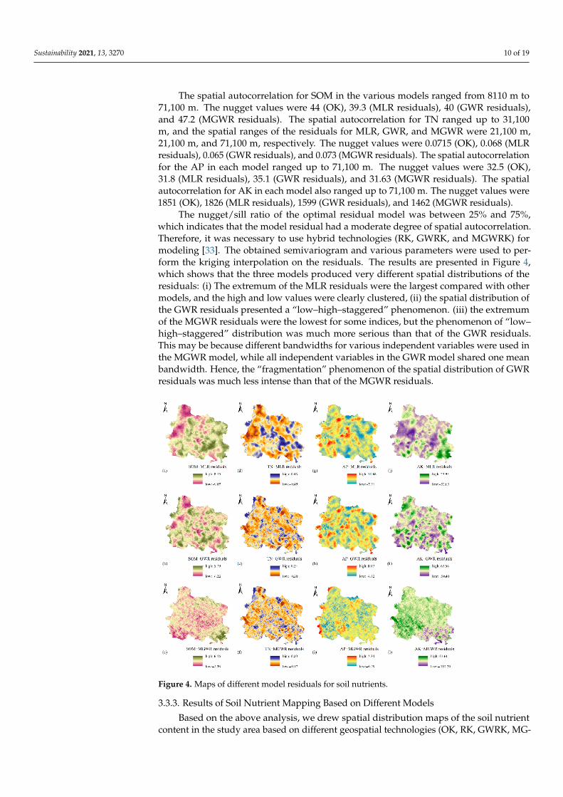
The nugget/sill ratio of the optimal residual model was between 25% and 75%,which indicates that the model residual had a moderate degree of spatial autocorrelation.Therefore, it was necessary to use hybrid technologies (RK, GWRK, and MGWRK) formodeling [33]. The obtained semivariogram and various parameters were used to per-form the kriging interpolation on the residuals. The results are presented in Figure 4,which shows that the three models produced very different spatial distributions of theresiduals: (i) The extremum of the MLR residuals were the largest compared with othermodels, and the high and low values were clearly clustered, (ii) the spatial distribution ofthe GWR residuals presented a “low–high–staggered” phenomenon. (iii) the extremumof the MGWR residuals were the lowest for some indices, but the phenomenon of “low–high–staggered” distribution was much more serious than that of the GWR residuals.This may be because different bandwidths for various independent variables were used inthe MGWR model, while all independent variables in the GWR model shared one meanbandwidth. Hence, the “fragmentation” phenomenon of the spatial distribution of GWRresiduals was much less intense than that of the MGWR residuals.

Figure 4. Maps of different model residuals for soil nutrients.

3.3.3. Results of Soil Nutrient Mapping Based on Different Models

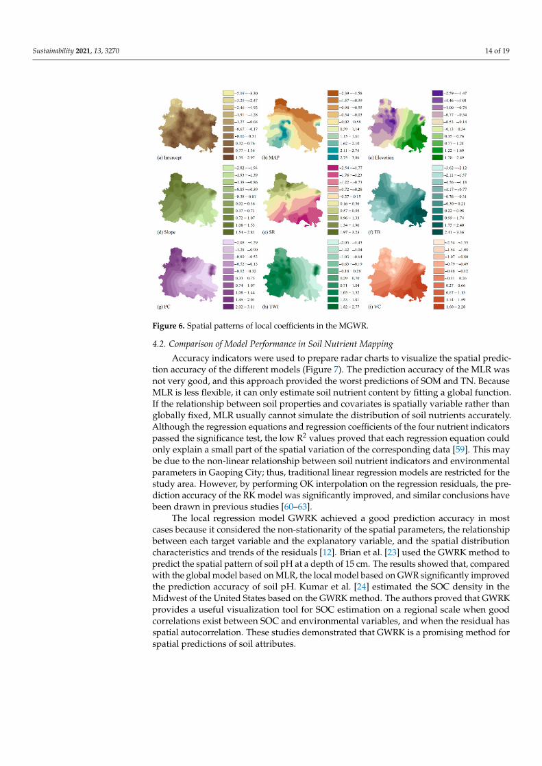
Based on the above analysis, we drew spatial distribution maps of the soil nutrientcontent in the study area based on different geospatial technologies (OK, RK, GWRK, MG-

Sustainability 2021, 13, 3270 11 of 19

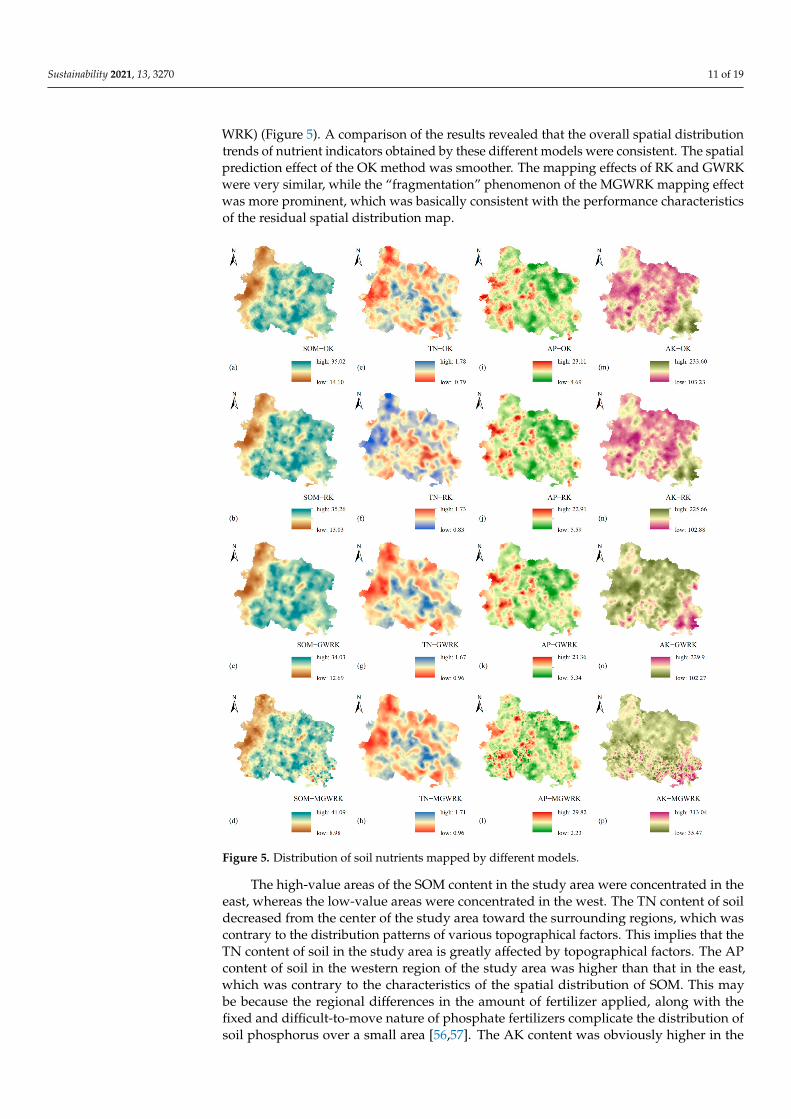
WRK) (Figure 5). A comparison of the results revealed that the overall spatial distributiontrends of nutrient indicators obtained by these different models were consistent. The spatialprediction effect of the OK method was smoother. The mapping effects of RK and GWRKwere very similar, while the “fragmentation” phenomenon of the MGWRK mapping effectwas more prominent, which was basically consistent with the performance characteristicsof the residual spatial distribution map.

Figure 5. Distribution of soil nutrients mapped by different models.

The high-value areas of the SOM content in the study area were concentrated in theeast, whereas the low-value areas were concentrated in the west. The TN content of soildecreased from the center of the study area toward the surrounding regions, which wascontrary to the distribution patterns of various topographical factors. This implies that theTN content of soil in the study area is greatly affected by topographical factors. The APcontent of soil in the western region of the study area was higher than that in the east,which was contrary to the characteristics of the spatial distribution of SOM. This maybe because the regional differences in the amount of fertilizer applied, along with thefixed and difficult-to-move nature of phosphate fertilizers complicate the distribution ofsoil phosphorus over a small area [56,57]. The AK content was obviously higher in the

Sustainability 2021, 13, 3270 12 of 19

southeast region of the study area compared to the northwest. The study also found thatthe soil nutrient content in the river valley is relatively high. This may be due to the flatterrain and convenient irrigation conditions, which is beneficial to the accumulation ofvarious soil nutrient contents while soil nutrients are more likely to be lost in mountainousand hilly areas. At the same time, human activities such as different main crops anddifferent management measures in various towns and small farm families may also causedifferences in the spatial pattern of soil nutrient content.

3.3.4. Evaluation of Model Accuracy

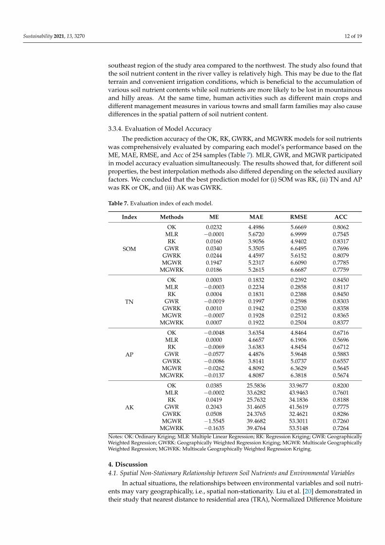
The prediction accuracy of the OK, RK, GWRK, and MGWRK models for soil nutrientswas comprehensively evaluated by comparing each model’s performance based on theME, MAE, RMSE, and Acc of 254 samples (Table 7). MLR, GWR, and MGWR participatedin model accuracy evaluation simultaneously. The results showed that, for different soilproperties, the best interpolation methods also differed depending on the selected auxiliaryfactors. We concluded that the best prediction model for (i) SOM was RK, (ii) TN and APwas RK or OK, and (iii) AK was GWRK.

Table 7. Evaluation index of each model.

Index Methods ME MAE RMSE ACC

SOM

OK 0.0232 4.4986 5.6669 0.8062MLR −0.0001 5.6720 6.9999 0.7545RK 0.0160 3.9056 4.9402 0.8317

GWR 0.0340 5.3505 6.6495 0.7696GWRK 0.0244 4.4597 5.6152 0.8079MGWR 0.1947 5.2317 6.6090 0.7785

MGWRK 0.0186 5.2615 6.6687 0.7759

TN

OK 0.0003 0.1832 0.2392 0.8450MLR −0.0003 0.2234 0.2858 0.8117RK 0.0004 0.1831 0.2388 0.8450

GWR −0.0019 0.1997 0.2598 0.8303GWRK 0.0010 0.1942 0.2530 0.8358MGWR −0.0007 0.1928 0.2512 0.8365

MGWRK 0.0007 0.1922 0.2504 0.8377

AP

OK −0.0048 3.6354 4.8464 0.6716MLR 0.0000 4.6657 6.1906 0.5696RK −0.0069 3.6383 4.8454 0.6712

GWR −0.0577 4.4876 5.9648 0.5883GWRK −0.0086 3.8141 5.0737 0.6557MGWR −0.0262 4.8092 6.3629 0.5645

MGWRK −0.0137 4.8087 6.3818 0.5674

AK

OK 0.0385 25.5836 33.9677 0.8200MLR −0.0002 33.6282 43.9463 0.7601RK 0.0419 25.7632 34.1836 0.8188

GWR 0.2043 31.4605 41.5619 0.7775GWRK 0.0508 24.3765 32.4621 0.8286MGWR −1.5545 39.4682 53.3011 0.7260

MGWRK −0.1635 39.4764 53.5148 0.7264Notes: OK: Ordinary Kriging; MLR: Multiple Linear Regression; RK: Regression Kriging; GWR: GeographicallyWeighted Regression; GWRK: Geographically Weighted Regression Kriging; MGWR: Multiscale GeographicallyWeighted Regression; MGWRK: Multiscale Geographically Weighted Regression Kriging.

4. Discussion4.1. Spatial Non-Stationary Relationship between Soil Nutrients and Environmental Variables

In actual situations, the relationships between environmental variables and soil nutri-ents may vary geographically, i.e., spatial non-stationarity. Liu et al. [20] demonstrated intheir study that nearest distance to residential area (TRA), Normalized Difference Moisture

Sustainability 2021, 13, 3270 13 of 19

Index (NDMI), slope, Normalized Difference Vegetation Index (NDVI), nearest distance toroad (TRD), and elevation were the dominant variables affecting the spatial distributionof SOC stocks; while the other three factors (i.e., nearest distance to river (TRR), aspect,and the land cover degree comprehensive index (LDCI)) did not play a dominant role inany part of the study region.

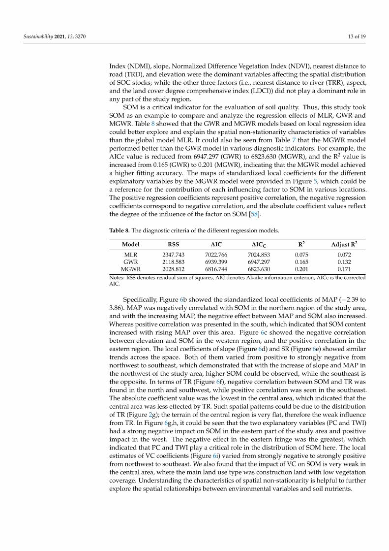
SOM is a critical indicator for the evaluation of soil quality. Thus, this study tookSOM as an example to compare and analyze the regression effects of MLR, GWR andMGWR. Table 8 showed that the GWR and MGWR models based on local regression ideacould better explore and explain the spatial non-stationarity characteristics of variablesthan the global model MLR. It could also be seen from Table 7 that the MGWR modelperformed better than the GWR model in various diagnostic indicators. For example, theAICc value is reduced from 6947.297 (GWR) to 6823.630 (MGWR), and the R2 value isincreased from 0.165 (GWR) to 0.201 (MGWR), indicating that the MGWR model achieveda higher fitting accuracy. The maps of standardized local coefficients for the differentexplanatory variables by the MGWR model were provided in Figure 5, which could bea reference for the contribution of each influencing factor to SOM in various locations.The positive regression coefficients represent positive correlation, the negative regressioncoefficients correspond to negative correlation, and the absolute coefficient values reflectthe degree of the influence of the factor on SOM [58].

Table 8. The diagnostic criteria of the different regression models.

Model RSS AIC AICC R2 Adjust R2

MLR 2347.743 7022.766 7024.853 0.075 0.072GWR 2118.583 6939.399 6947.297 0.165 0.132

MGWR 2028.812 6816.744 6823.630 0.201 0.171Notes: RSS denotes residual sum of squares, AIC denotes Akaike information criterion, AICc is the correctedAIC.

Specifically, Figure 6b showed the standardized local coefficients of MAP (−2.39 to3.86). MAP was negatively correlated with SOM in the northern region of the study area,and with the increasing MAP, the negative effect between MAP and SOM also increased.Whereas positive correlation was presented in the south, which indicated that SOM contentincreased with rising MAP over this area. Figure 6c showed the negative correlationbetween elevation and SOM in the western region, and the positive correlation in theeastern region. The local coefficients of slope (Figure 6d) and SR (Figure 6e) showed similartrends across the space. Both of them varied from positive to strongly negative fromnorthwest to southeast, which demonstrated that with the increase of slope and MAP inthe northwest of the study area, higher SOM could be observed, while the southeast isthe opposite. In terms of TR (Figure 6f), negative correlation between SOM and TR wasfound in the north and southwest, while positive correlation was seen in the southeast.The absolute coefficient value was the lowest in the central area, which indicated that thecentral area was less effected by TR. Such spatial patterns could be due to the distributionof TR (Figure 2g); the terrain of the central region is very flat, therefore the weak influencefrom TR. In Figure 6g,h, it could be seen that the two explanatory variables (PC and TWI)had a strong negative impact on SOM in the eastern part of the study area and positiveimpact in the west. The negative effect in the eastern fringe was the greatest, whichindicated that PC and TWI play a critical role in the distribution of SOM here. The localestimates of VC coefficients (Figure 6i) varied from strongly negative to strongly positivefrom northwest to southeast. We also found that the impact of VC on SOM is very weak inthe central area, where the main land use type was construction land with low vegetationcoverage. Understanding the characteristics of spatial non-stationarity is helpful to furtherexplore the spatial relationships between environmental variables and soil nutrients.

Sustainability 2021, 13, 3270 14 of 19

Figure 6. Spatial patterns of local coefficients in the MGWR.

4.2. Comparison of Model Performance in Soil Nutrient Mapping

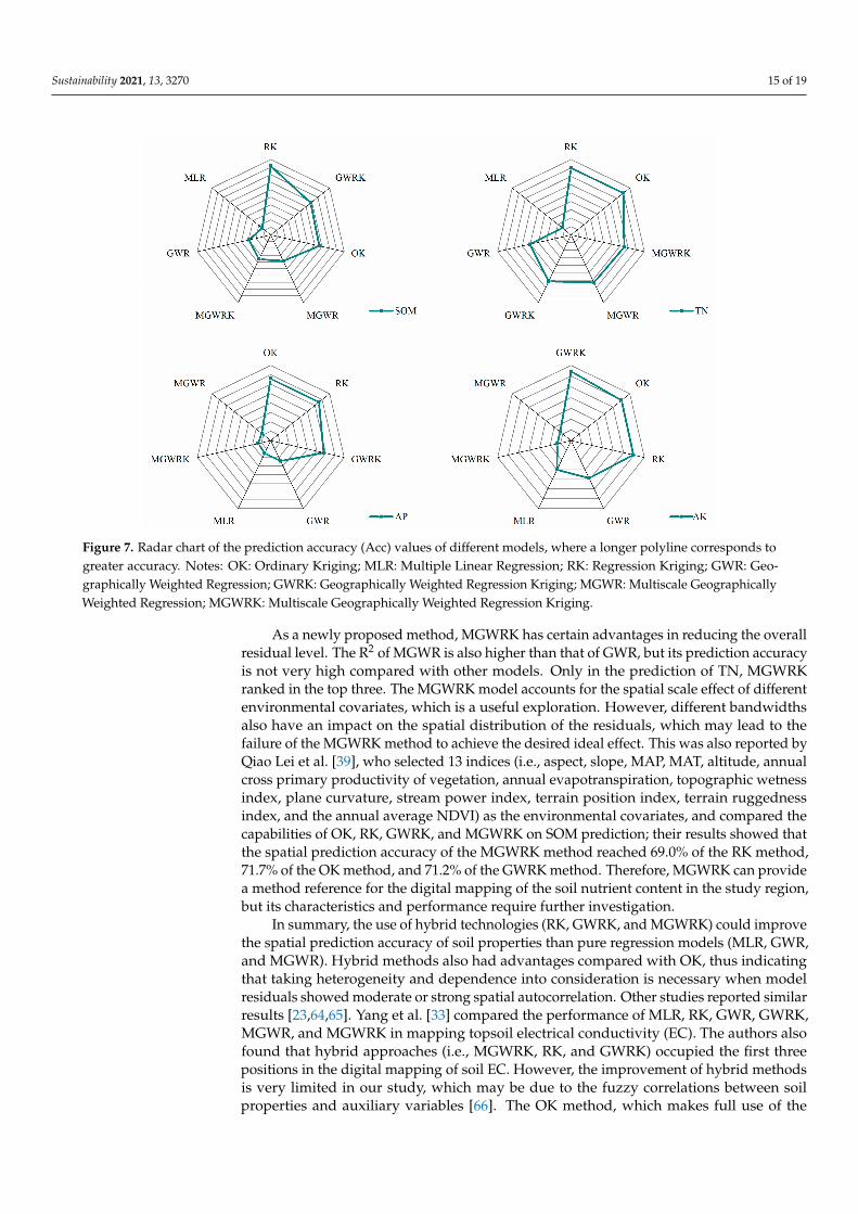
Accuracy indicators were used to prepare radar charts to visualize the spatial predic-tion accuracy of the different models (Figure 7). The prediction accuracy of the MLR wasnot very good, and this approach provided the worst predictions of SOM and TN. BecauseMLR is less flexible, it can only estimate soil nutrient content by fitting a global function.If the relationship between soil properties and covariates is spatially variable rather thanglobally fixed, MLR usually cannot simulate the distribution of soil nutrients accurately.Although the regression equations and regression coefficients of the four nutrient indicatorspassed the significance test, the low R2 values proved that each regression equation couldonly explain a small part of the spatial variation of the corresponding data [59]. This maybe due to the non-linear relationship between soil nutrient indicators and environmentalparameters in Gaoping City; thus, traditional linear regression models are restricted for thestudy area. However, by performing OK interpolation on the regression residuals, the pre-diction accuracy of the RK model was significantly improved, and similar conclusions havebeen drawn in previous studies [60–63].

The local regression model GWRK achieved a good prediction accuracy in mostcases because it considered the non-stationarity of the spatial parameters, the relationshipbetween each target variable and the explanatory variable, and the spatial distributioncharacteristics and trends of the residuals [12]. Brian et al. [23] used the GWRK method topredict the spatial pattern of soil pH at a depth of 15 cm. The results showed that, comparedwith the global model based on MLR, the local model based on GWR significantly improvedthe prediction accuracy of soil pH. Kumar et al. [24] estimated the SOC density in theMidwest of the United States based on the GWRK method. The authors proved that GWRKprovides a useful visualization tool for SOC estimation on a regional scale when goodcorrelations exist between SOC and environmental variables, and when the residual hasspatial autocorrelation. These studies demonstrated that GWRK is a promising method forspatial predictions of soil attributes.

Sustainability 2021, 13, 3270 15 of 19

Figure 7. Radar chart of the prediction accuracy (Acc) values of different models, where a longer polyline corresponds togreater accuracy. Notes: OK: Ordinary Kriging; MLR: Multiple Linear Regression; RK: Regression Kriging; GWR: Geo-graphically Weighted Regression; GWRK: Geographically Weighted Regression Kriging; MGWR: Multiscale GeographicallyWeighted Regression; MGWRK: Multiscale Geographically Weighted Regression Kriging.

As a newly proposed method, MGWRK has certain advantages in reducing the overallresidual level. The R2 of MGWR is also higher than that of GWR, but its prediction accuracyis not very high compared with other models. Only in the prediction of TN, MGWRKranked in the top three. The MGWRK model accounts for the spatial scale effect of differentenvironmental covariates, which is a useful exploration. However, different bandwidthsalso have an impact on the spatial distribution of the residuals, which may lead to thefailure of the MGWRK method to achieve the desired ideal effect. This was also reported byQiao Lei et al. [39], who selected 13 indices (i.e., aspect, slope, MAP, MAT, altitude, annualcross primary productivity of vegetation, annual evapotranspiration, topographic wetnessindex, plane curvature, stream power index, terrain position index, terrain ruggednessindex, and the annual average NDVI) as the environmental covariates, and compared thecapabilities of OK, RK, GWRK, and MGWRK on SOM prediction; their results showed thatthe spatial prediction accuracy of the MGWRK method reached 69.0% of the RK method,71.7% of the OK method, and 71.2% of the GWRK method. Therefore, MGWRK can providea method reference for the digital mapping of the soil nutrient content in the study region,but its characteristics and performance require further investigation.

In summary, the use of hybrid technologies (RK, GWRK, and MGWRK) could improvethe spatial prediction accuracy of soil properties than pure regression models (MLR, GWR,and MGWR). Hybrid methods also had advantages compared with OK, thus indicatingthat taking heterogeneity and dependence into consideration is necessary when modelresiduals showed moderate or strong spatial autocorrelation. Other studies reported similarresults [23,64,65]. Yang et al. [33] compared the performance of MLR, RK, GWR, GWRK,MGWR, and MGWRK in mapping topsoil electrical conductivity (EC). The authors alsofound that hybrid approaches (i.e., MGWRK, RK, and GWRK) occupied the first threepositions in the digital mapping of soil EC. However, the improvement of hybrid methodsis very limited in our study, which may be due to the fuzzy correlations between soilproperties and auxiliary variables [66]. The OK method, which makes full use of the

Sustainability 2021, 13, 3270 16 of 19

spatial structure information of the data, has also achieved a satisfactory accuracy at a highsampling density and with a strong spatial correlation of the sampled data. Therefore,it may be more beneficial to design soil sampling rationally and obtain higher-qualitydata of auxiliary variables than to look for complex statistical methods to improve spatialprediction accuracy [10,67].

5. Conclusions

To summarize, this study compared the performance of OK, MLR, RK, GWR, GWRK,MGWR, and MGWRK for the digital mapping of soil nutrients in Gaoping City, China.The results showed that these models performed differently when predicting various in-dicators. The hybrid methods (RK, GWRK, and MGWRK) improved model predictionaccuracy to a certain extent when the residuals were spatially correlated; however, thisimprovement was not significant. The new method MGWRK has certain advantages inreducing the overall residual level, but it failed to achieve the desired accuracy. Further ver-ification of the applicable conditions and deviations of the MGWRK approach is required.Considering the cost of modeling, the OK method still provided an interpolation methodwith a relatively simple analysis process and relatively reliable results. This does not meanthat more complex models would lead to an improved model performance.

In addition, the prediction accuracy of a spatial regression model largely dependson the correct selection of auxiliary variables. Although all the variables selected in thisstudy were natural factors, soil nutrients are simultaneously affected by five major soil-forming factors and human factors. Human activities in low-altitude areas increase thespatial variability of soil nutrients. Future research should select appropriate methods toquantify management measures (e.g., planting systems, farming measurements), and thenincorporate them into models to further improve prediction accuracy.

Author Contributions: Conceptualization, L.G.; methodology, L.G. and L.Q.; software, L.G. andG.W.; validation, L.G. and L.Q.; formal analysis, G.W. and X.Z.; investigation, L.G. and L.Q.; re-sources, W.Z.; data curation, L.G.; writing—original draft preparation, L.G.; writing—review andediting, W.Z. and L.G.; visualization, L.G.; supervision, W.Z.; project administration, W.Z. and M.H.;funding acquisition, W.Z. and M.H. All authors have read and agreed to the published version of themanuscript.

Funding: This research was funded by the Major Research Plan of Shanxi Province, China, grantnumber 201703D211002-2.

Institutional Review Board Statement: Not applicable.

Informed Consent Statement: Not applicable.

Data Availability Statement: Publicly available datasets were analyzed in this study. These data canbe found here: http://data.cma.cnr (acceded on 15 October 2020); http://www.gscloud.cn (accededon 15 October 2020).

Acknowledgments: The authors thank the reviewers for their helpful comments.

Conflicts of Interest: The authors declare no conflict of interest. The funders had no role in the designof the study; in the collection, analyses, or interpretation of data; in the writing of the manuscript, orin the decision to publish the results.

References1. Mcbratney, A.B.; Odeh, I.O.A.; Bishop, T.F.A.; Dunbar, M.S.; Shatar, T.M. An overview of pedometric techniques for use in soil

survey. Geoderma 2000, 97, 293–327. [CrossRef]2. Sumfleth, K.; Duttmann, R. Prediction of soil property distribution in paddy soil landscapes using terrain data and satellite

information as indicators. Ecol. Indic. 2008, 8, 485–501. [CrossRef]3. John, K.; Isong, I.A.; Kebonye, N.M.; Ayito, E.O.; Agyeman, P.C.; Afu, S.M. Using Machine Learning Algorithms to Estimate

Soil Organic Carbon Variability with Environmental Variables and Soil Nutrient Indicators in an Alluvial Soil. Land 2020, 9, 487.[CrossRef]

Sustainability 2021, 13, 3270 17 of 19

4. Liu, D.; Wang, Z.; Zhang, B.; Song, K.; Duan, H. Spatial distribution of soil organic carbon and analysis of related factors incroplands of the black soil region, Northeast China. Agric. Ecosyst. Environ. 2006, 113, 73–81. [CrossRef]

5. Liu, E.; Yan, C.; Mei, X.; He, W.; Bing, S.H.; Ding, L.; Qin, L.; Shuang, L.; Fan, T. Long-term effect of chemical fertilizer, straw, andmanure on soil chemical and biological properties in northwest China. Geoderma 2010, 158, 173–180. [CrossRef]

6. Cambardella, C.; Moorman, T.B.; Novak, J.M.; Parkin, T.B.; Konopka, A. Field-Scale Variability of Soil Properties in Central IowaSoils. Soilence Soc. Am. J. 1994, 58, 1501–1511. [CrossRef]

7. Wang, K.; Zhang, C.; Li, W. Comparison of Geographically Weighted Regression and Regression Kriging for Estimating theSpatial Distribution of Soil Organic Matter. Mapp. Sci. Remote Sens. 2012, 49, 915–932. [CrossRef]

8. Emadi, M.; Baghernejad, M. Comparison of spatial interpolation techniques for mapping soil pH and salinity in agriculturalcoastal areas, northern Iran. Arch. Agron. Soil Sci. 2014, 60, 1315–1327. [CrossRef]

9. Ye, H.; Huang, W.; Huang, S.; Huang, Y.; Zhang, S.; Dong, Y.; Chen, P. Effects of different sampling densities on geographicallyweighted regression kriging for predicting soil organic carbon. Spat. Stat. 2017, 20, 76–91. [CrossRef]

10. Shen, Q.; Wang, Y.; Wang, X.; Liu, X.; Zhang, X.; Zhang, S. Comparing interpolation methods to predict soil total phosphorus inthe Mollisol area of Northeast China. Catena 2019, 174, 59–72. [CrossRef]

11. Eldeiry, A.A.; Garcia, L.A. Comparison of Ordinary Kriging, Regression Kriging, and Cokriging Techniques to Estimate SoilSalinity Using LANDSAT Images. J. Irrig. Drain. Eng. 2010, 136, 355–364. [CrossRef]

12. Kumar, A.; Lal, R.; Liu, D. A geographically weighted regression kriging approach for mapping soil organic carbon stock.Geoderma 2012, 189–190, 627–634. [CrossRef]

13. Watt, M.S.; Palmer, D.J. Use of regression kriging to develop a Carbon: Nitrogen ratio surface for New Zealand. Geoderma 2012,183–184, 49–57. [CrossRef]

14. Bangroo, S.; Najar, G.; Achin, E.; Truong, P.N. Application of predictor variables in spatial quantification of soil organic carbonand total nitrogen using regression kriging in the North Kashmir forest Himalayas. Catena 2020, 193, 104632. [CrossRef]

15. Mondal, A.; Khare, D.; Kundu, S.; Mondal, S.; Mukherjee, S.; Mukhopadhyay, A. Spatial soil organic carbon (SOC) prediction byregression kriging using remote sensing data. Egypt. J. Remote Sens. Space Sci. 2017, 20, 61–70. [CrossRef]

16. Odeh, I.O.; McBratney, A.B.; Chittleborough, D.J. Further results on prediction of soil properties from terrain attributes: Hetero-topic cokriging and regression-kriging. Geoderma 1995, 67, 215–226. [CrossRef]

17. Hengl, T.; Heuvelink, G.B.; Stein, A. A generic framework for spatial prediction of soil variables based on regression-kriging.Geoderma 2004, 120, 75–93. [CrossRef]

18. Hengl, T.; Heuvelink, G.B.M.; Rossiter, D.G. About regression-kriging: From equations to case studies. Comput. Geosci. 2007, 33,1301–1315. [CrossRef]

19. Walter, C.; Mcbratney, A.B.; Donuaoui, A.; Minasny, B. Spatial prediction of topsoil salinity in the Chelif Valley, Algeria, usinglocal ordinary kriging with local variograms versus whole-area variogram. Soil Res. 2001, 39, 259–272. [CrossRef]

20. Liu, Y.; Guo, L.; Jiang, Q.; Zhang, H.; Chen, Y. Comparing geospatial techniques to predict SOC stocks. Soil Tillage Res. 2015, 148,46–58. [CrossRef]

21. Brunsdon, C.; Fotheringham, A.S.; Charlton, M.E. Geographically Weighted Regression: A Method for Exploring SpatialNonstationarity. Geogr. Anal. 1996, 28, 281–298. [CrossRef]

22. Kumar, S.; Lal, R. Mapping the organic carbon stocks of surface soils using local spatial interpolator. J. Environ. Monit. JEM 2011,13, 3128–3135. [CrossRef]

23. Odhiambo, B.O.; Kenduiywo, B.K.; Were, K. Spatial prediction and mapping of soil pH across a tropical afro-montane landscape.Appl. Geogr. 2020, 114, 102129. [CrossRef]

24. Kumar, S. Estimating spatial distribution of soil organic carbon for the Midwestern United States using historical database.Chemosphere 2015, 127, 49–57. [CrossRef] [PubMed]

25. Mitran, T.; Mishra, U.; Lal, R.; Ravisankar, T.; Sreenivas, K. Spatial distribution of soil carbon stocks in a semi-arid region of India.Geoderma Reg. 2018, 15, e00192. [CrossRef]

26. Yu, H.; Fotheringham, A.S.; Li, Z.; Oshan, T.; Kang, W.; Wolf, L.J. Inference in multiscale geographically weighted regression.Geogr. Anal. 2020, 52, 87–106. [CrossRef]

27. Mcmaster, R.B.; Sheppard, E. Introduction: Scale and Geographic Inquiry; Blackwell Publishing Ltd.: Hoboken, NJ, USA, 2008.28. Lam, N.S.N.; Quattrochi, D.A. On the Issues of Scale, Resolution, and Fractal Analysis in the Mapping Sciences. Prof. Geogr. 1992,

44, 88–98. [CrossRef]29. Peng, G.; Ling, B. Scale Effects on Spatially Embedded Contact Networks. Comput. Environ. Urban Syst. 2016, 59, 142–151.

[CrossRef]30. Cao, C. Detecting the Scale and Resolution Effects in Remote Sensing and GIS; Louisiana State University and Agricultural &

Mechanical College: Baton Rouge, LA, USA, 1992.31. Pan, Y.; Roth, A.; Yu, Z.; Doluschitz, R. The impact of variation in scale on the behavior of a cellular automata used for land use

change modeling. Comput. Environ. Urban Syst. 2010, 34, 400–408. [CrossRef]32. Murakami, D.; Lu, B.; Harris, P.; Brunsdon, C.; Charlton, M.; Nakaya, T.; Griffith, D.A. The importance of scale in spatially

varying coefficient modeling. Ann. Am. Assoc. Geogr. 2019, 109, 50–70. [CrossRef]

Sustainability 2021, 13, 3270 18 of 19

33. Yang, S.-H.; Liu, F.; Song, X.-D.; Lu, Y.-Y.; Li, D.-C.; Zhao, Y.-G.; Zhang, G.-L. Mapping topsoil electrical conductivity by a mixedgeographically weighted regression kriging: A case study in the Heihe River Basin, northwest China. Ecol. Indic. 2019, 102,252–264. [CrossRef]

34. Mei, C.L.; He, S.Y.; Fang, K.T. A Note on the Mixed Geographically Weighted Regression Model. J. Reg. Sci. 2004, 44, 143–157.[CrossRef]

35. McMillen, D.P. Geographically Weighted Regression: The Analysis of Spatially Varying Relationships. Am. J. Agric. Econ. 2004,86, 554–556. [CrossRef]

36. Nakaya, T.; Fotheringham, S.; Charlton, M.; Brunsdon, C. Semiparametric Geographically Weighted Generalised Linear Modellingin GWR 4.0. 2009. Available online: http://www.geocomputation.org/2009/PDF/nakaya_et_al.pdf (accessed on 15 October2020).

37. Wu, C.; Ren, F.; Hu, W.; Du, Q. Multiscale geographically and temporally weighted regression: Exploring the spatiotemporaldeterminants of housing prices. Int. J. Geogr. Inf. Sci. 2019, 33, 489–511. [CrossRef]

38. Fotheringham, A.S.; Yang, W.; Wei, K. Multiscale Geographically Weighted Regression (MGWR). Ann. Am. Assoc. Geogr. 2017,107, 1247–1265. [CrossRef]

39. Qiao, L.; Zhang, W.; Huang, M.; Wang, G.; Ren, J. Mapping of soil organic matter and its driving factors study based on MGWRK.Sci. Agric. Sin. 2020, 53, 1830–1844. [CrossRef]

40. Carter, M.R.; Gregorich, E.G. Soil Sampling and Methods of Analysis; CRC Press: Boca Raton, FL, USA, 2007.41. Yang, S.; Zhang, H.; Zhang, C.; Li, W.; Guo, L.; Chen, J. Predicting soil organic matter content in a plain-to-hill transition belt

using geographically weighted regression with stratification. Arch. Agron. Soil Sci. 2019, 65, 1745–1757. [CrossRef]42. Zeng, C.; Yang, L.; Zhu, A.X.; Rossiter, D.G.; Liu, J.; Liu, J.; Qin, C.; Wang, D. Mapping soil organic matter concentration at

different scales using a mixed geographically weighted regression method. Geoderma 2016, 281, 69–82. [CrossRef]43. National Meteorological Information Center. Available online: http://data.cma.cnr (accessed on 15 October 2020).44. Geospatial Data Cloud. Available online: http://www.gscloud.cn (accessed on 15 October 2020).45. Shabrina, Z.; Buyuklieva, B.; Ng, M.K.M. Short-Term Rental Platform in the Urban Tourism Context: A Geographically Weighted

Regression (GWR) and a Multiscale GWR (MGWR) Approaches. Geogr. Anal. 2020, 1–22. [CrossRef]46. Oshan, T.M.; Li, Z.; Kang, W.; Wolf, L.J.; Fotheringham, A.S. MGWR: A Python Implementation of Multiscale Geographically

Weighted Regression for Investigating Process Spatial Heterogeneity and Scale. Int. J. Geo Inf. 2019, 8, 269. [CrossRef]47. Sun, Y.S.; Wang, W.F.; Li, G.C. Spatial distribution of forest carbon storage in Maoershan region, Northeast China based on

geographically weighted regression kriging model. Chin. J. Appl. Ecol. 2019, 30, 1642–1650. [CrossRef]48. Wang, S.; Hu, K.; Lu, P.; Yu, T. Spatial variability of soil available phosphorus and environmental risk analysis of soil phosphorus

in Pinggu County of Beijing. Sci. Agric. Sin. 2009, 42, 1290–1298. [CrossRef]49. Wang, S.; Adhikari, K.; Wang, Q.; Jin, X.; Li, H. Role of environmental variables in the spatial distribution of soil carbon (C),

nitrogen (N), and C:N ratio from the northeastern coastal agroecosystems in China. Ecol. Indic. Integr. Monit. Assess. Manag. 2018,84, 263–272. [CrossRef]

50. Tu, C.; He, T.; Lu, X.; Luo, Y.; Smith, P. Extent to which pH and topographic factors control soil organic carbon level in dry farmingcropland soils of the mountainous region of Southwest China. Catena 2018, 163, 204–209. [CrossRef]

51. Song, X.D.; Brus, D.J.; Liu, F.; Li, D.C.; Zhao, Y.G.; Yang, J.L.; Zhang, G.L. Mapping soil organic carbon content by geographicallyweighted regression: A case study in the Heihe River Basin, China. Geoderma 2016, 261, 11–12. [CrossRef]

52. Naipal, V.; Ciais, P.; Wang, Y.; Lauerwald, R.; Oost, K.V. Global soil organic carbon removal by water erosion underclimate changeand land use change during 1850–2005 AD. Biogeosci. Discuss. 2018, 4459–4480. [CrossRef]

53. Davidson, E.A.; Janssens, I.A. Temperature sensitivity of soil carbon decomposition and feedbacks to climate change. Nature 2006,440, 165–173. [CrossRef] [PubMed]

54. Schillaci, C.; Acutis, M.; Lombardo, L.; Lipani, A.; Fantappiè, M.; Märker, M.; Saia, S. Spatio-temporal topsoil organic carbonmapping of a semi-arid Mediterranean region: The role of land use, soil texture, topographic indices and the influence of remotesensing data to modelling. Sci. Total Environ. 2017, 601–602, 821–832. [CrossRef]

55. Agostinelli, C. Robust stepwise regression. J. Appl. Stat. 2003, 48, 557–558. [CrossRef]56. Behera, S.K.; Singh, M.V.; Singh, K.N.; Todwal, S. Distribution variability of total and extractable zinc in cultivated acid soils of

India and their relationship with some selected soil properties. Geoderma 2012, 162, 242–250. [CrossRef]57. Zhao, Q.; Zhao, G.; Jiang, H. Study on spatial variability of soil nutrients and reasonable sampling number at county scale. J. Nat.

Resour. 2012, 27, 1382–1391. [CrossRef]58. Qu, M.; Li, W.; Zhang, C.; Huang, B.; Zhao, Y. Spatial assessment of soil nitrogen availability and varying effects of related main

soil factors on soil available nitrogen. Environ. Sci. Process. Impacts 2016, 18, 1449–1457. [CrossRef] [PubMed]59. Hengl, T. A Practical Guide to Geostatistical Mapping of Environmental Variables; European Commission, Joint Research Centre,

Institute for Environment and Sustainability: Ispra, Italy, 2007.60. Zhang, S.; Wang, Z.; Zhang, B.; Song, K.; Liu, D.; Li, F.; Ren, C.; Huang, J.; Zhang, H. Prediction of spatial distribution of soil

nutrients using terrain attributes and remote sensing data. Trans. Chin. Soc. Agric. Eng. 2010, 26, 188–194. [CrossRef]61. Ren, L.; Yang, L.; Wang, H.; Yang, F.; Chen, W.; Zhang, L.; Jinhao, X.U. Spatial prediction of soil organic matter in apple region

based on random forest. Resour. Environ. Arid Region 2018. [CrossRef]

Sustainability 2021, 13, 3270 19 of 19

62. Yang, Q.; Wang, X.Q.; Sun, X.L.; Wang, H.L. Comparing Prediction Accuracies of Ordinary Kriging and Regression Kriging withREML in Soil Properties Mapping. Chin. J. Soil Sci. 2018, 49, 283–292. [CrossRef]

63. Ziadat, M.F. Analyzing Digital Terrain Attributes to Predict Soil Attributes for a Relatively Large Area. Soil Sci. Soc. Am. J. 2005,69, 1590–1599. [CrossRef]

64. Benítez, F.L.; Anderson, L.O.; Formaggio, A.N.R. Evaluation of geostatistical techniques to estimate the spatial distributionof aboveground biomass in the Amazon rainforest using high-resolution remote sensing data. Acta Amaz. 2016, 46, 151–160.[CrossRef]

65. Imran, M.; Stein, A.; Zurita-Milla, R. Using geographically weighted regression kriging for crop yield mapping in West Africa.Int. J. Geogr. Inf. Syst. 2015, 29, 234–257. [CrossRef]

66. Kravchenko, A.N.; Robertson, G.P. Can Topographical and Yield Data Substantially Improve Total Soil Carbon Mapping byRegression Kriging? Agron. J. 2007, 99, 12–17. [CrossRef]

67. Zhang, C.-T.; Yang, Y. Can the spatial prediction of soil organic matter be improved by incorporating multiple regressionconfidence intervals as soft data into BME method? Catena 2019, 178, 322–334. [CrossRef]