TECHNISCHE UNIVERSITÄT MÜNCHEN Fachgebiet für Genomorientierte Bioinformatik Comparative proteomics – methods and applications Thorsten Sven-Olaf Schmidt Vollständiger Abdruck der von der Fakultät Wissenschaftszentrum Weihenstephan für Ernährung, Landnutzung und Umwelt der Technischen Universität München zur Erlangung des akademischen Grades eines Doktor der Naturwissenschaften genehmigten Dissertation. Vorsitzender: Univ.-Prof. B. Küster, Ph.D. Prüfer der Dissertation: 1. Univ.-Prof. Dr. D. Frischmann 2. Univ.-Prof. Dr. H.-W. Mewes 3. Univ.-Prof. Dr. J. Parsch, (Ludwig-Maximilians-Universität München) Die Dissertation wurde am 19.6.2008 bei der Technischen Universität München eingereicht und durch die Fakultät Wissenschaftszentrum Weihenstephan für Ernährung, Landnutzung und Umwelt am 23.10.2008 angenommen.

Welcome message from author
This document is posted to help you gain knowledge. Please leave a comment to let me know what you think about it! Share it to your friends and learn new things together.
Transcript
TECHNISCHE UNIVERSITÄT MÜNCHEN
Fachgebiet für Genomorientierte Bioinformatik
Comparative proteomics – methods and applications
Thorsten Sven-Olaf Schmidt Vollständiger Abdruck der von der Fakultät Wissenschaftszentrum Weihenstephan für Ernährung, Landnutzung und Umwelt der Technischen Universität München zur Erlangung des akademischen Grades eines
Doktor der Naturwissenschaften genehmigten Dissertation.
Vorsitzender: Univ.-Prof. B. Küster, Ph.D. Prüfer der Dissertation: 1. Univ.-Prof. Dr. D. Frischmann
2. Univ.-Prof. Dr. H.-W. Mewes 3. Univ.-Prof. Dr. J. Parsch, (Ludwig-Maximilians-Universität München)
Die Dissertation wurde am 19.6.2008 bei der Technischen Universität München eingereicht und durch die Fakultät Wissenschaftszentrum Weihenstephan für Ernährung, Landnutzung und Umwelt am 23.10.2008 angenommen.
ii
Table of Contents
ZUSAMMENFASSUNG ........................................................................................................... IV
CHAPTER 1 MOTIVATION AND OVERVIEW ................................................................... 6
1.1 GENOME SEQUENCING AND ANNOTATION ............................................................................ 7 1.2 PROTEOMIC MEASUREMENTS ............................................................................................... 8 1.3 GENOME STRUCTURE ........................................................................................................... 9 1.4 COMPARATIVE GENOMICS AND PROTEOMICS IN THE SPACE OF GENE ATTRIBUTES ............. 10 1.5 LACK OF SOFTWARE TOOLS ................................................................................................ 12 1.6 THESIS OUTLINE ................................................................................................................. 13
CHAPTER 2 DATA INTEGRATION, MAPPING AND STATISTICAL ANALYSES ... 15
2.1 PROMPT – PROTEIN MAPPING AND COMPARISON ............................................................ 15
2.1.1 Introduction ............................................................................................................... 15 2.1.2 Material and Methods ............................................................................................... 16 2.1.3 Applications ............................................................................................................... 32 2.1.4 Discussion ................................................................................................................. 39
2.2 INTEGRATION OF FUNCTIONAL AND PHYSICAL ANNOTATIONS ............................................ 40
2.2.1 Introduction ............................................................................................................... 40 2.2.2 Material and Methods ............................................................................................... 41 2.2.3 Results ....................................................................................................................... 43
CHAPTER 3 APPLICATIONS IN COMPARATIVE PROTEOMICS ............................. 45
3.1 DATABASES AND RETRIEVAL SYSTEMS .............................................................................. 45
3.1.1 PEDANT-Webservices ............................................................................................... 45 3.1.2 CORUM- Search and EJB accession ........................................................................ 50
3.2 COMPARATIVE ANALYSES FOR STRUCTURAL BIOINFORMATICS .......................................... 52
3.2.1 Background ............................................................................................................... 52 3.2.2 Material and Methods ............................................................................................... 53 3.2.3 Results ....................................................................................................................... 56
iii
3.3 COMPLEX FUNCTIONAL PROFILING OF PROTEIN AND GENE SETS ......................................... 57
3.3.1 Introduction ............................................................................................................... 57 3.3.2 Methods and Implementation .................................................................................... 58 3.3.3 Results ....................................................................................................................... 59 3.3.4 Discussion ................................................................................................................. 64
CHAPTER 4 GENE AND PROTEIN EXPRESSION .......................................................... 65
4.1 ABUNDANCE PROFILING OF THE E.COLI PROTEOME ............................................................ 65
4.1.1 Introduction ............................................................................................................... 65 4.1.2 Material and Methods ............................................................................................... 66 4.1.3 Results ....................................................................................................................... 72 4.1.4 Discussion ................................................................................................................. 87
4.2 GENOME ARCHITECTURES AND EVALUATION ..................................................................... 88
4.2.1 Introduction ............................................................................................................... 88 4.2.2 Material and Methods ............................................................................................... 89 4.2.3 Results ....................................................................................................................... 93 4.2.4 Discussion ............................................................................................................... 109
CHAPTER 5 CONCLUSIONS AND FUTURE WORK .................................................... 110
SUMMARY .............................................................................................................................. 111
LIST OF TABLES ................................................................................................................... 113
LIST OF FIGURES ................................................................................................................. 114
BIBLIOGRAPHY .................................................................................................................... 116
ACKNOWLEDGEMENTS ..................................................................................................... 130
APPENDIX ............................................................................................................................... 131
PUBLICATIONS ....................................................................................................................... 131 TEACHING EXERCISES ............................................................................................................ 135 CURRICULUM VITAE ............................................................................................................... 137

iv
Zusammenfassung
Schwerpunkt dieser Arbeit ist die Entwicklung von Bioinformatikmethoden sowie deren Anwendung in der vergleichenden Proteomik. Dabei werden die hier neu entwickelten Methoden (Schmidt and Frishman 2006; Antonov, Schmidt et al. 2008; Schmidt and Frishman 2008) auf biologische Fragestellungen angewandt und die Ergebnisse präsentiert (Riley, Schmidt et al. 2005; Schmidt and Frishman 2006; Smialowski, Schmidt et al. 2006; Riley, Schmidt et al. 2007; Ruepp, Brauner et al. 2007; Schmidt, Hombach et al. 2007; Antonov, Schmidt et al. 2008; Irmler, Hartl et al. 2008; Ishihama, Schmidt et al. 2008; Schmidt and Frishman 2008). Die Arbeit gliedert sich – neben einer Einführung und Hintergrundinformation in Kapitel eins - in drei thematische Abschnitte: Kapitel zwei stellt das PROMPT Framework zur vergleichenden Analyse von biologischen Daten insbesondere aus dem Gebiet der Genomik und Proteomik (Schmidt and Frishman 2006) vor. Dabei werden für das häufige Problem der korrekten Zuordnung von Identifiern (dem sogenannten Mapping) sowie für die Integration von funktionellen, strukturellen und weiteren Proteineigenschaften neu entwickelte Lösungen und deren Nutzen präsentiert (Irmler, Hartl et al. 2008; Ishihama, Schmidt et al. 2008). Um die volle Mächtigkeit der in dieser Arbeit entwickelten, evaluierten und angewandten Methoden nutzen zu können, ist eine solide Datenbasis unabdingbar. Zusätzlich werden daher im Rahmen dieser Arbeit Datenbanken und Retrieval Systeme, basierend auf Web Service und J2EE Technologien, entwickelt und vorgestellt (Riley, Schmidt et al. 2005; Riley, Schmidt et al. 2007; Ruepp, Brauner et al. 2007). Kapitel drei gibt hierzu eine kurze Übersicht. Darüber hinaus wird in Kapitel drei demonstriert, wie mittels der eingeführten Datenbanksysteme im Zusammenspiel mit den vorgestellten Methoden - komplexe Funktionen besser beschrieben werden können (Antonov, Schmidt et al. 2008) und ein prediktives Modell hinsichtlich Proteinkristallisierbarkeit erstellt werden kann (Smialowski, Schmidt et al. 2006). In Kapitel vier werden die entwickelten Methoden erstmals in großem Umfang auf Protein-Abundanz Daten angewandt. Im ersten Teil von Kapitel vier werden neue biologische Erkenntnisse im Hinblick auf Funktion, Struktur und weiterer Aspekte in E.coli vorgestellt (Ishihama, Schmidt et al. 2008).
v
Im zweiten Teil von Kapitel vier, wird darüber hinaus die zugrunde liegende Genomarchitektur von höheren Eukaryoten analysiert. Dabei konnten nicht nur Gemeinsamkeiten und Unterschiede zwischen Organismen und Methoden gezeigt werden (Schmidt, Hombach et al. 2007), sondern zusätzlich eine neue Konsensusmethode zur Vorhersage von Isochore-Genomstrukturen für alle vollständig sequenzierten Vetebratengenome etabliert werden (Schmidt and Frishman 2008). Kapitel fünf fasst die wichtigsten Erkenntnisse der Forschungsarbeiten zusammen und gibt einen Ausblick für weitere Fragestellungen. Jedes Kapitel beginnt mit einer Beschreibung des relevanten spezifischen Hintergrundwissens und beschreibt die entwickelten Methoden sowie die Anwendungen und erzielten Ergebnisse.
Chapter 1 Motivation and Overview
Deciphering the mechanisms of any human disease needs a comprehensive analysis of the underlying biological system. For example, complex illnesses like cancer need to be targeted by taking proteomic-, genomic- as well as time- and spatial interplays into account. Threatening viral pandemics, like avian influenza and SARS, require iterated host-pathogen-inference analysis, hypothesis generation and evaluation with experimental- as well as bioinformatics approaches. Moreover, epigenetic - as well as individual- differences will raise the need of further personalized medicine. Bioinformatics modeling of cellular systems promises a solution of these challenges, but clearly depends on a satisfactory amount of knowledge and methods. Although current genomic as well as proteomic high-throughput and large-scale experiments are generating a flood of data, a multitude of essential issues are open yet. For example, protein structure crystallization experiments are seriously hindered by unpredictable outcomes. Moreover, the modeling of biological networks and further exploration of functional modules is hampered by the lack of quantitative information. Beyond, functional analysis of expression data is limited in ways to describe complex functions and relationships and expression analysis usually remains behind its possibilities by neglecting available information like protein structures. Additionally, even trivial data integration tasks are significantly delayed by incompatible formats, identifiers and interfaces. Moreover, general bioinformatics frameworks and methods for basic comparative analyses hardly exist. To put all in a nutshell, biological interdependencies and interactions need a broad system-wide analysis, based upon solid data integration and analysis. In this work, we addressed the outlined questions. We provide new bioinformatics methods for data integration and comparative analysis on the level of genome and proteome data (Schmidt and Frishman 2006; Schmidt and Frishman 2006; Schmidt, Hombach et al. 2007; Schmidt and Frishman 2008). Applying our developed technology, we further revealed novel insights of biological functions and finally provide new data resources and interfaces for free public usage (Riley, Schmidt et al. 2005; Smialowski, Schmidt et al. 2006; Riley, Schmidt et al. 2007; Ruepp, Brauner et al. 2007; Schmidt, Hombach et al. 2007; Antonov, Schmidt et al. 2008; Irmler, Hartl et al. 2008; Ishihama, Schmidt et al. 2008; Schmidt and Frishman
1.1 Genome sequencing and annotation
7
2008). In the following parts of this chapter, an overview of the basic background of each facet is given. Finally an outline of this thesis is presented at the end of this chapter.
1.1 Genome sequencing and annotation
Progress in DNA sequencing and data management made in the last years has generated a wealth of information usable in many scientific fields. Presently, more than 330 annotated genomes are available in the PEDANT database (Riley, Schmidt et al. 2005; Riley, Schmidt et al. 2007) and other data sources like UniProt (Bairoch, Apweiler et al. 2005), EMBL (Kanz, Aldebert et al. 2005) and CORUM (Ruepp, Brauner et al. 2007). Multiple levels of annotation e.g. gene, domain, structure and ontologies like Gene-Ontology and FunCat provide a pledora of data; for a detailed review of the current state of databases and annotations a comprehensive review is given by Frishman (2007). Unfortunately, analysis of the increasingly growing data is complicated by a number of factors. Firstly, knowledge from different resources is not accessible in a standardized way. For example, processing simple sequence information from different sources like GenBank (Benson, Karsch-Mizrachi et al. 2005) entries and Swiss-Prot (Gasteiger, Jung et al. 2001) files needs different parsers. Secondly, linking information of interest together is essential but hampered by differing names and identifiers, e.g. the same gene of Escherichia coli can be referenced in different sources with Blattner-IDs (Blattner, Plunkett et al. 1997), GenBank identifiers or by UniProt entry names. Finally, software to compare protein sets is virtually nonexistent. In addition to large-scale sequencing and automated annotation pipelines, high-through-put technologies like expression arrays and proteomic determination technologies provide a new plethora of data. Current proteomic measurements are in range not only to identify proteins as such, but provide additional information like posttranslational modifications, protein interactions and insights of quantitative protein copy numbers. In consequence proteomics is already discussed to be the “New Genomics” (Cox and Mann 2007). The following section gives a basic introduction into proteomic technology with a focus on estimating protein abundance levels which were used throughout this work. Beyond, detailed guidelines about proteomics experiments and a recent critical review with regard to quantitative proteomics are discussed by Wilkins et al. (2006) and Bantscheff et al. (2007).
1.2 Proteomic measurements
8
1.2 Proteomic measurements
Mass spectrometry (MS), in combination with protein and peptide separation methods, allows the efficient qualitative identification of proteins in complex mixtures. As an alternative to two-dimensional gel electrophoresis (2-DE) and mass spectrometric analysis of the resulting individual spots, shotgun approaches have been developed as suitable tools for large scale proteome analysis (Link, Eng et al. 1999; Peng, Elias et al. 2003). These are based on protease digestion of the sample as a whole and subsequent peptide separation and identification by multidimensional LC-MS/MS. However, in contrast to the 2-DE approaches, information about protein abundances is initially unavailable in the shotgun approaches. Relative quantification for abundance comparison of the same protein in different samples can be realized by incorporation of stable isotopes into the samples (Gygi, Rist et al. 1999; Oda, Huang et al. 1999; Mirgorodskaya, Kozmin et al. 2000) which is utilized in methods like cICAT (Hansen, Schmitt-Ulms et al. 2003), iTRAQTM (Ross, Huang et al. 2004), 18O-labeling (Mirgorodskaya, Kozmin et al. 2000) or SILAC (Ong, Blagoev et al. 2002). Relative changes in concentration of the same protein between different experimental setups can be very accurately determined by these methods, but a major disadvantage is the absence of a direct measure of protein concentrations. Abundance comparison of different proteins is hence not possible. Several mass spectrometric strategies have been reported to overcome this limitation. The more traditional ones utilize internal standards, e.g. spiking the complex mixture with peptides of known concentration (Barr, Maggio et al. 1996; Gerber, Rush et al. 2003), and typically require calibration for each protein to be quantified. A more recently introduced method describes a new parameter to express protein concentrations without the need of introducing labels or internal standards. It is calculated from the averaged ion intensities of the three most intense tryptic peptides per protein, as extracted from the ion current chromatograms. This parameter is called ‘xPAI’ for ‘extracted ion intensity-based protein abundance index’. It has been shown to correlate well with known protein concentrations in the human RNA polymerase II complex (Rappsilber, Ishihama et al. 2003) and rat mitochondria (Forner, Foster et al. 2006). However, xPAI is limited to samples of low complexity since selection of only the three most intense peptides becomes unreliable with an increasing number of different proteins in the sample. Additionally, it is difficult to apply the xPAI approach to samples which were pre-fractionated at the peptide level, due to carry-over effects between the different fractions. A similar method has been described using an alternate scanning LCMS method (LCMS(E)), which is available on certain mass spectrometer instruments (Silva, Gorenstein et al. 2006). Here, all peaks in the MS spectra are selected as precursor ions for subsequent MS/MS scans resulting in lower peak intensity dependence of peptide identification as is the case for conventional data-dependent MS/MS scans. If the MS device allows this kind of
1.3 Genome structure
9
detection mode it is preferable to xPAI, but it is still presented with the mentioned basic challenges of this approach. Other label free ways of large scale protein quantification by MS make use of correlations between the number of actually identified tryptic peptides per protein and the theoretical number of tryptic peptides (Rappsilber, Ryder et al. 2002), or the molecular weight of the proteins (Sanders, Jennings et al. 2002). These ratios have been termed ‘protein abundance index’ (PAI). More recently, we found empirically that PAI correlates better with the logarithm of protein concentration and defined an exponentially modified PAI (emPAI) (Ishihama, Oda et al. 2005). Although such a method of concentration determination may not be expected to be overly precise, the accuracy of emPAI-derived concentration measurements has been shown to lie within an error range of only a factor of maximally 3.4 for 46 proteins in whole cell lysates of murine neuroblastoma (N2A) cells (Ishihama, Oda et al. 2005) and is therefore in the same range or better than protein concentration measurements based on staining methods. A major advantage is that the emPAI based protein concentration is automatically and quickly available for all proteins identified by MS without the need of any additional experimental setup. A similar approach was reported recently for the membrane proteome of S. cerevisiae, where protein concentrations were estimated by using the number of obtained spectra per protein divided by the length of the protein (Zybailov, Mosley et al. 2006). In this work, we used an approach to maximize MS based proteome identification coverage in an application to the E. coli cytosol, in combination with a reliable and quick concentration estimation of the identified proteins. We thus provide data as well as novel significant associations between abundance and protein properties. In addition to an analysis of proteins, we address underlying genomic properties. The direct dependency of biological systems from their genome commits to take all available information under account. For example, recently it was shown that the “genome landscape” of hosts is related to the codon usage of bacteriaphages (Lucks, Nelson et al. 2008). Especially higher organisms as plants and mammalian genomes show specific and clear genome structures. The next section provides a brief overview of the history and of biological properties found to be associated with genome structures.
1.3 Genome structure
More than three decades ago gradient density analyses of fragmented DNA identified long fairly compositionally homogenous regions on mammalian chromosomes, widely known as isochores (Filipski, Thiery et al. 1973; Macaya, Thiery et al. 1976; Thiery, Macaya et al. 1976) or long homogeneous genome
1.4 Comparative genomics and proteomics in the space of gene attributes
10
regions (LHGRs) (Oliver, Carpena et al. 2002), associated with a wide range of important biological properties. Gene density is up to 16 times higher in GC-rich isochores than in GC-poor isochores (Mouchiroud, D'Onofrio et al. 1991), and the genes in the high GC-isochores code for shorter proteins and are more compact with a smaller amount of introns (Duret, Mouchiroud et al. 1995). It was also shown, that the GC-rich codons, such as those coding for alanine and arginine, are more frequent in GC-rich isochores (D'Onofrio, Mouchiroud et al. 1991; Clay, Caccio et al. 1996). The distribution of repeat elements is influenced by the isochore structure of the genome: SINE (short-interspersed nuclear element) sequences tend to be more frequent in GC-rich isochores while the LINE (long-interspersed nuclear elements) sequences are preferentially found in GC-poorer regions (Meunier-Rotival, Soriano et al. 1982; Soriano, Meunier-Rotival et al. 1983; Jabbari and Bernardi 1998). The structure of chromosome bands also correlates with isochores: T-bands predominantly consist of GC-rich isochores, while the GC-poorer isochores are found in G-bands (Saccone, De Sario et al. 1992; Saccone, De Sario et al. 1993; Costantini, Clay et al. 2006). The recombination frequency is higher (Eisenbarth, Beyer et al. 2000; Fullerton, Bernardo Carvalho et al. 2001) and the replication starts up to two hours earlier (Tenzen, Yamagata et al. 1997) in regions with high GC-content. Taking all information on the genomic as well as on the proteomic levels together is destinated to provide further insights into intra- and inter-cellular modes of operations. In the following two sections we will firstly give an overview of here applied comparative approaches and secondly outline the need of general bioinformatic frameworks addressing such problem domains.
1.4 Comparative genomics and proteomics in the space of gene attributes
Molecular bioinformatics was born as a science of comparing individual DNA and amino acid sequences with each other. Over the past three decades important biological insights have been obtained by establishing unexpected sequence similarity between seemingly unrelated proteins e.g. (Koonin, Altschul et al. 1996). More recently, modern high-throughput technologies (genome sequencing, expression profiling, mass spectrometry) injected tremendous amounts of sequence data and associated experimental information into the public databases, creating the need for collective comparisons of large sequence groups (e.g., whole proteomes). The transition from pairwise sequence comparison to comparing large protein datasets against each other is similar to switching from finding differences between individuals to comparing populations of whole countries. Is wine consumption in
1.4 Comparative genomics and proteomics in the space of gene attributes
11
France higher than in England? Do Germans drive faster than Americans? Analogous queries applied to biological molecules prevail in post-genomic bioinformatics. In many genome sequencing papers one finds a bar chart contrasting the new sequence with other genomes in terms of sequence motif composition. While analysing gene clusters obtained by expression analysis it is typical to ask whether one gene group is significantly enriched in certain functional categories with respect to another one. Are proteins with many interaction partners different from less prolific interactors (Pagel, Mewes et al. 2004)? Are essential genes more evolutionary conserved than non-essential ones (Jordan, Rogozin et al. 2002)? The list of such questions is endless. Answering some of them involves a mere counting exercise while others require the application of sophisticated bioinformatics approaches and careful statistical analyses. Mining protein properties at large scale has been especially productive in computational structural genomics where it helped to establish basic facts about structural complements encoded in complete genomes. For example, it was shown that membrane proteins constitute roughly 30% of each proteome (Frishman and Mewes 1997). The patterns of globular fold occurrence in different organism groups were carefully investigated (Gerstein 1997). The mechanisms of protein structure adaptation to extreme environments were revealed by comparing the genomes of thermophilic (Thompson and Eisenberg 1999; Das and Gerstein 2000), halophilic (Kennedy, Ng et al. 2001), psychrophilic (Gianese, Bossa et al. 2002), and barophilic (Di Giulio 2005) species with their counterparts living under normal conditions. Large-scale comparison of protein datasets has the impact to answer a multitude of scientific questions. For example what distinguish crystallizable and non- crystallizable proteins, essential and non-essential ones or abundant and non-abundant proteins? What characterize interactions vs. non interactors, soluble vs. non-soluble, disease related vs. non-disease related, GroEL substrates vs. non-GroEL substrates? For instance, it was shown that the GroEL obligate protein prefer to fold into a TIM-Barrel structure (Kerner, Naylor et al. 2005), translate faster and show a lower folding propensity (Noivirt-Brik, Unger et al. 2007) than non-GroEL substrates. The realm of open questions is almost endless and only restricted by the number of attributes and the amount of available data. In general one would like to compare two or more sets of proteins or genes. These two sets may result of different experiments or of distinct protein groups. Common of such analyses is that – instead of comparing the properties of two single entities – whole populations can be compared.

1.5 Lack of software tools
12
1.5 Lack of software tools
One recurrent bioinformatics task in comparative proteomics involves mapping and integrating information from disparate sources. While reporting experimental results as well as theoretical predictions one may refer to proteins using the UniProt (Bairoch, Apweiler et al. 2005), GenBank (Benson, Karsch-Mizrachi et al. 2005), or RefSeq (Pruitt, Tatusova et al. 2005) nomenclature, or custom IDs for sequences not yet submitted to public databases. The situation is additionally complicated by frequent genome updates which may result in new, previously missed ORFs identified, existing sequences corrected, as well as the removal of misannotated ORFs. As a result, establishing unambiguous correspondence between protein sequence entries and associated experimental data may represent a difficult, albeit trivial challenge. Countless customized software tools with varying degrees of complexity have been independently written in research labs throughout the world to address protein comparison and mapping tasks, although there are significant commonalities in the technical steps that need to be implemented. The authors of this contribution, too, wrote their share of throw-away perl scripts and quick-shot Java programs to compare GroEL substrates with the rest of the Escherichia coli lysate (Kerner, Naylor et al. 2005), crystallizable and non-crystallizable proteins (Smialowski, Schmidt et al. 2006), disease-associated proteins and those without such association (Wong, Fritz et al. 2005), abundant and non-abundant proteins (Ishihama, Schmidt et al. 2008), as well as completely sequenced genomes (Frishman, Albermann et al. 2001) and functional properties of alternatively spliced genes (Neverov, Artamonova et al. 2005). It is precisely the fatigue from re-inventing the wheel over and over again that motivated us to develop a bioinformatics framework for large-scale protein comparisons. Much to our surprise, we realized that general solutions for comparing and analysing large sets of proteins in the space of arbitrary annotation attributes are currently hardly available or limited to certain application areas. We are aware of only two software projects addressing the need for large scale comparative analysis. The comprehensive Genome Properties resource (Haft, Selengut et al. 2005) allows comparing complete prokaryotic genomes based on a multitude of pre-defined property assertions. The system is primarily focused on metabolic information, does not allow user-supplied protein attributes, does not provide statistical tests to validate differences between genomes, and is not available for local installation. GeneMerge (Castillo-Davis and Hartl 2003) is an excellent tool for detecting over-representation of certain functional or categorical descriptors in a given subset of proteins relative to the general set based on rigorous statistical tests, but it provides neither integration with bioinformatics databases nor a graphical user interface.
1.6 Thesis Outline
13
1.6 Thesis Outline
The completion of the sequencing of several mammalian genomes as well as advances in the large-scale measurement of gene expression on transcript and protein levels provide the basis for the emerging field of systems biology. A major challenge towards a comprehensive analysis of biological systems is the integration of data from different “omics” sources and their interpretation on a functional level. In chapter 2, we describe a new platform-independent system named PROMPT (Protein Mapping and Comparison Tool) capable of addressing a wide spectrum of routine tasks in comparative proteomics (Schmidt and Frishman 2006). PROMPT enables the user to compare arbitrary protein sequence sets, revealing statistically significant differences in their annotation features. Protein annotation can be imported from a variety of standard bioinformatics databases as well as from generic XML description files. Facilities are provided for linking experimental information obtained from different sources to appropriate genes despite discrepancies in gene identifiers and minor sequence variation. The entire functionality of the system is available via a full-featured server-independent graphical user interface. At the same time, a Java API is provided for integration with user applications. In chapter 2.2 we demonstrate the advantages of the PROMPT software suite for comparative proteomics by analyzing physical features of regulated gene products from multiple databases (Irmler, Hartl et al. 2008). Chapter 3, starts with a brief description of contributions to the databases PEDANT and CORUM and data retrivial systems that were developed in the context of this work (Riley, Schmidt et al. 2005; Riley, Schmidt et al. 2007; Ruepp, Brauner et al. 2007). In the second section of chapter 3, the the power of comparative proteomics is demonstrated by confronting proteins yielding crystal structures with non-crystallizable proteins (Smialowski, Schmidt et al. 2006). We present newly identified sequence-based features that can predict the outcome of a crystallization experiment with high accuracy. As even small advantages in the field of experimental structure determination directly respond in remarkable time and resource savings a computational estimation of the crystallizability under given experimental settings is very helpful for structure determination experiments. In the third part of chapter three, we extend the comparative approach to a higher level of complexity. In addition to comparing single gene and protein attributes combinations of such information may result in more informative statements. In analogy of a natural language we introduce operators like AND, OR and EXCLUDE to combine annotation terms. Thus, connecting all single functions with operators reveals the previously hidden interplay and relationships. Moreover, we present a web-based service named ProfCom implementing this method. Finally, we
1.6 Thesis Outline
14
demonstrate that ProfCom surpasses current state-of-the-art functional profiling methods and give examples of newly revealed complex functions of genes in multiple human cancer types. We discuss new insights beyond existing co-occurrence approaches into the functions of up-regulated genes in various cancer samples (Antonov, Schmidt et al. 2008). Chapter 4 builds upon all previous chapters and is based on the data resources, integration and methodology developed in this work. In the first part of chapter 4, we present abundance measurements for more than 1000 E.coli proteins and present new significant relations between protein abundance and the properties and functions of proteins. Thus, we give novel insights into the role of protein levels in this model organism. Moreover, we show associations between genetic properties like localization in operons and protein abundance (Ishihama, Schmidt et al. 2008). This leads directly to the inclusion of genome properties and to a more wholistic view of biological systems. In the second part, we present a new method for fully automated isochore assignments. Isochores are long genomic regions with fairly homogenous GC content and were firstly described by ultra-centrifugation experiments (Bernardi 1989). Isochores represent a “fundamental level of genome organization” (Eyre-Walker and Hurst 2001) and are associated with multiple biological properties and epigenetic programming (Vinogradov 2005; Schmegner, Hameister et al. 2007). Several algorithms for compositional segmentation of genomic sequences have recently been proposed. In the second section of chapter 4, we show that although the currently available isochore mapping methods agree on the isochore classification of about two thirds of the human DNA, they produce significantly different results with regard to the location of isochore boundaries and isochore length distribution. We present a new consensus isochore assignment method based on a majority voting and evaluate it against the currently available body of isochore knowledge. The isochores derived by the consensus approach correlate higher with the distribution of gene density and experimental evidence than individual methods. We provide a measure of the isochore assignment confidence based on the number of methods that agree for a given base pair and demonstrate how the confidence depends on GC content and the distance to isochore border regions. Moreover, we provide IsoBase - a comprehensive on-line database of isochore maps for all completely sequenced vertebrate genomes - that enables the user to evaluate statistical distributions of isochore properties and compare isochore assignments between organisms and methods. Finally, chapter 5 gives a concise summary and outlook of this thesis. Each chapter starts with a brief introduction and presents the used methodology in detail. In addition to a general discussion of the results in chapter 5, all results are depicted and discussed exhaustively within the respective chapter.
Chapter 2 Data integration, mapping and statistical analyses
Comparison of large protein datasets has become a standard task in bioinformatics. Typically researchers wish to know whether one group of proteins is significantly enriched in certain annotation attributes or sequence properties compared to another group, and whether this enrichment is statistically significant. In order to conduct such comparisons it is often required to integrate molecular sequence data and experimental information from disparate incompatible sources. While many specialized programs exist for comparisons of this kind in individual problem domains, such as expression data analysis, no generic solution capable of addressing a wide spectrum of routine tasks in comparative proteomics was available yet. In this chapter we present PROMPT – A protein mapping and comparison tool (Schmidt and Frishman 2006). We further show how genomic and proteomic data can be integrated and complemented using the PROMPT software suite (Irmler, Hartl et al. 2008).
2.1 PROMPT – Protein Mapping and Comparison
2.1.1 Introduction
Although a multitude of software is available that calculates many protein features like the Biology Workbench (Subramaniam 1998), solutions to compare and analyse arbitrary sets of proteins are hardly available or limited to narrow application areas. For example, the recently published GenomeProperties (Haft, Selengut et al. 2005) service allows relating various protein properties, but is limited to the investigation of whole prokaryotic genomes and does not provide statistical tests to validate differences or similarities between the genomes. Another approach, the GeneMerge (Castillo-Davis and Hartl 2003) algorithm evades limitations to predefined datasets by requesting a custom input format, and thus shifting the responsibility of data integration to the user. Nevertheless, large scale automatic comparison of protein sets is gaining more and more impact since the amount of biological data is increasing rapidly and manual in-
2.1 PROMPT – Protein Mapping and Comparison
16
depth analysis is not possible in the majority of cases. In particular a multitude of new insights have been achieved due to comparative studies. For example, mechanisms of thermal adaptations have been revealed by comparative genomics showing major factors for protein stability (Thompson and Eisenberg 1999; Das and Gerstein 2000; Saunders, Thomas et al. 2003). Other application domains of comparative analyses are structural and functional genomics. For illustration, Proteome Analyst (Lu, Szafron et al. 2004) predicts functional assignments or sub cellular localizations based on a Support Vector Machine (SVM) classifier utilizing differences in sets of proteins. A similar approach is used in SVM-Prot (Cai, Han et al. 2003), which classifies proteins based on their primary sequence into functional categories.
2.1.2 Material and Methods
Functional overview
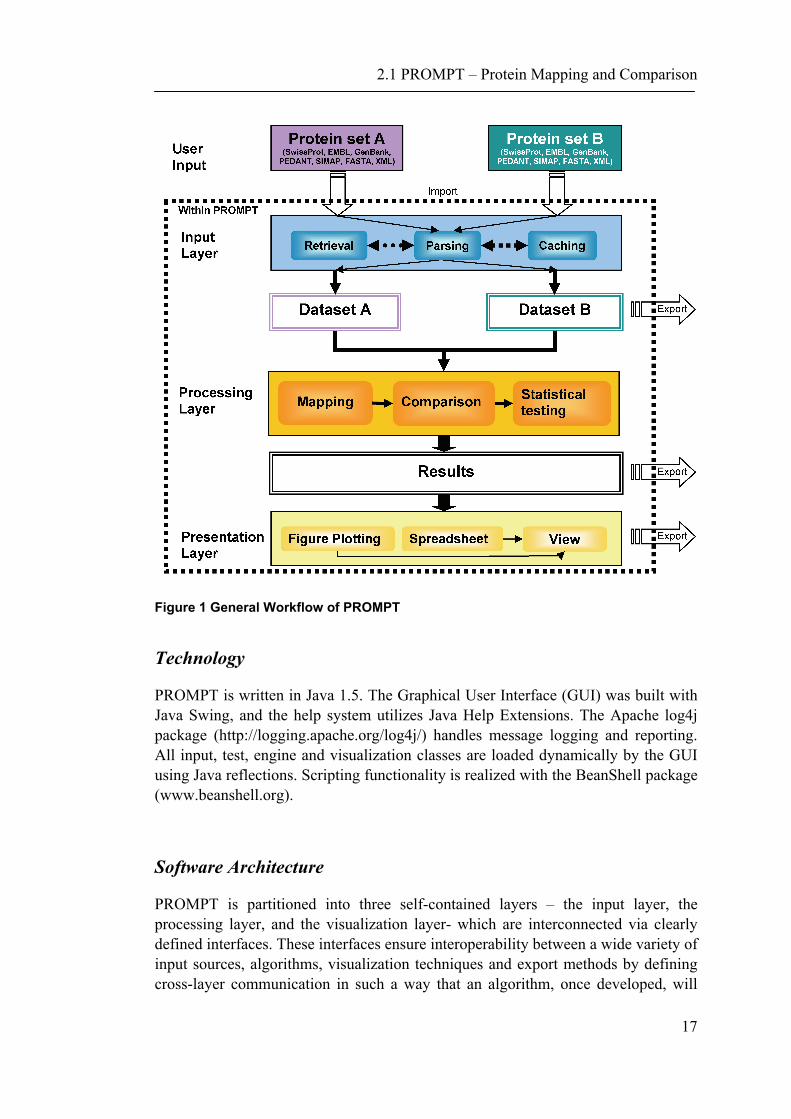
PROMPT operates with three types of information associated with proteins: database IDs, amino acid sequences, and annotation attributes. The latter may be any protein feature manually assigned, experimentally measured, or calculated from sequence; such features may be nominal and/or numeric. Examples of numeric features are molecular weight, pI, abundance, and the number of interaction partners. Nominal features can be sequence motifs, keywords, functional categories, EC numbers, and so on. Sequences are primarily used by PROMPT to establish the correspondence between proteins imported from different sources and thus having incompatible database IDs. This is done by similarity-based mapping and careful handling of exceptions and minor sequence variations. Sequence data can be either obtained directly from public databases, or supplied by the user as flat files using one of the commonly accepted formats as well as a custom XML format. Once annotation features have been imported and assigned to appropriate proteins, actual large scale comparisons of protein properties, data interpretation, and statistical analyses can be conducted. The central task consists of comparing two sets of proteins and finding significantly enriched or depleted features in one of the sets. Results can be viewed in tabular form, visualized by various types of plots, and exported to other applications. As seen in Figure 1, a general PROMPT workflow involves three stages: i) data import, ii) data processing which includes mapping, comparison, and statistical tests, and iii) visualization and presentation of results for subsequent analyses. Additionally, the data can be exported and saved at each step.
2.1 PROMPT – Protein Mapping and Comparison
17
Figure 1 General Workflow of PROMPT
Technology
PROMPT is written in Java 1.5. The Graphical User Interface (GUI) was built with Java Swing, and the help system utilizes Java Help Extensions. The Apache log4j package (http://logging.apache.org/log4j/) handles message logging and reporting. All input, test, engine and visualization classes are loaded dynamically by the GUI using Java reflections. Scripting functionality is realized with the BeanShell package (www.beanshell.org).
Software Architecture
PROMPT is partitioned into three self-contained layers – the input layer, the processing layer, and the visualization layer- which are interconnected via clearly defined interfaces. These interfaces ensure interoperability between a wide variety of input sources, algorithms, visualization techniques and export methods by defining cross-layer communication in such a way that an algorithm, once developed, will

2.1 PROMPT – Protein Mapping and Comparison
18
work with any input module that provides the requested input interface. It does not matter, for example, whether the sequence data comes from a local UniProt XML file (Bairoch, Apweiler et al. 2005), an SQL database or a Web service. This approach allows the application of PROMPT’s algorithms to new and currently unknown data formats and sources. Conversely, newly added algorithms can immediately reuse all of the available input and output modules. The same applies to new import modules that can be used with all applicable algorithms as soon as the required interfaces have been implemented. Similar to the approach adopted in Java Beans (Cochrane, Aldebert et al. 2006) all PROMPT modules are encapsulated by the troika of Init, Run, and GetResults methods that perform initialization, actual computation and the returning of results, respectively. This design pattern provides a comfortable and uniform handling of all parts of the PROMPT framework. Furthermore, the clear separation between individual layers ensures reproducibility of results as the data can be saved and evaluated at every step. An overview of PROMPT’s software architecture is shown in Figure 2.
Figure 2 PROMPT Software architecture.
PROMPT is based on a three-layered architecture namely an input-layer, a processing layer and a visualization layer. The input layer is responsible for reading
2.1 PROMPT – Protein Mapping and Comparison
19
and importing data from a wide variety of sources. The classes of the processing layer are in charge of doing the actual analysis work. Here calculations are performed and statistical tests applied. Finally the visualization layer is responsible for creating figures and presenting results. All layers are independently from each other, but can interact with each other seamlessly by interfaces. Instances of the input layer act as Data Accession Objects (DAOs) and provide methods to access the input independently of the input format or source. New algorithms or input formats can be easily added by implementing, and if desired extending, the respective interfaces. By inheriting from the basic input-interfaces third party parts can be used immediately within the graphical user interface and benefit from the existing framework. Furthermore as long as the interfaces are not changed, the current implementation can be modified without any need to update code that is using the framework objects.
Data retrieval and integration
Data import from flat files is predominantly based on BioJava (Castillo-Davis and Hartl 2003) which is used to parse multi-FASTA, EMBL (Cochrane, Aldebert et al. 2006), Genbank (Benson, Karsch-Mizrachi et al. 2005), and UniProt (Bairoch, Apweiler et al. 2005) formats. In particular, the UniProt XML format is supported. Additionally, data can be directly imported from two MIPS databases - PEDANT (Frishman, Albermann et al. 2001) and SIMAP (Rattei, Arnold et al. 2006) – using data access objects provided by these two resources. User extensions can be easily incorporated by creating Java classes that implement or extend the Java interfaces provided by PROMPT.
2.1 PROMPT – Protein Mapping and Comparison
20
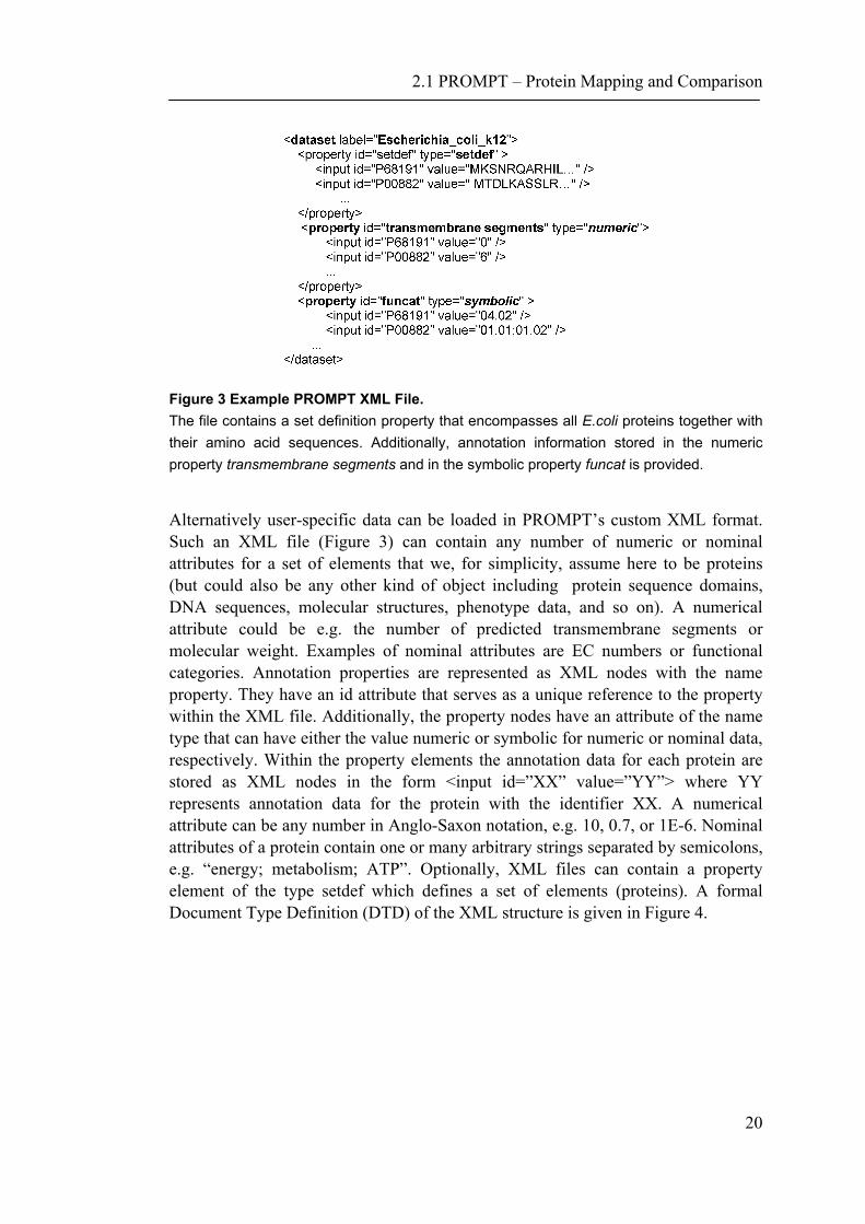
Figure 3 Example PROMPT XML File. The file contains a set definition property that encompasses all E.coli proteins together with their amino acid sequences. Additionally, annotation information stored in the numeric property transmembrane segments and in the symbolic property funcat is provided.
Alternatively user-specific data can be loaded in PROMPT’s custom XML format. Such an XML file (Figure 3) can contain any number of numeric or nominal attributes for a set of elements that we, for simplicity, assume here to be proteins (but could also be any other kind of object including protein sequence domains, DNA sequences, molecular structures, phenotype data, and so on). A numerical attribute could be e.g. the number of predicted transmembrane segments or molecular weight. Examples of nominal attributes are EC numbers or functional categories. Annotation properties are represented as XML nodes with the name property. They have an id attribute that serves as a unique reference to the property within the XML file. Additionally, the property nodes have an attribute of the name type that can have either the value numeric or symbolic for numeric or nominal data, respectively. Within the property elements the annotation data for each protein are stored as XML nodes in the form <input id=”XX” value=”YY”> where YY represents annotation data for the protein with the identifier XX. A numerical attribute can be any number in Anglo-Saxon notation, e.g. 10, 0.7, or 1E-6. Nominal attributes of a protein contain one or many arbitrary strings separated by semicolons, e.g. “energy; metabolism; ATP”. Optionally, XML files can contain a property element of the type setdef which defines a set of elements (proteins). A formal Document Type Definition (DTD) of the XML structure is given in Figure 4.
2.1 PROMPT – Protein Mapping and Comparison
21
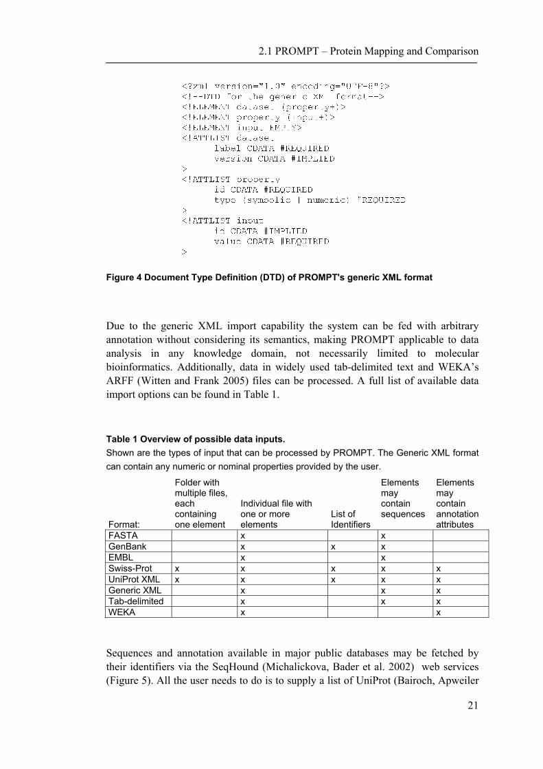
Figure 4 Document Type Definition (DTD) of PROMPT's generic XML format
Due to the generic XML import capability the system can be fed with arbitrary annotation without considering its semantics, making PROMPT applicable to data analysis in any knowledge domain, not necessarily limited to molecular bioinformatics. Additionally, data in widely used tab-delimited text and WEKA’s ARFF (Witten and Frank 2005) files can be processed. A full list of available data import options can be found in Table 1.
Table 1 Overview of possible data inputs. Shown are the types of input that can be processed by PROMPT. The Generic XML format can contain any numeric or nominal properties provided by the user.
Format:
Folder with multiple files, each containing one element
Individual file with one or more elements
List of Identifiers
Elements may contain sequences
Elements may contain annotation attributes
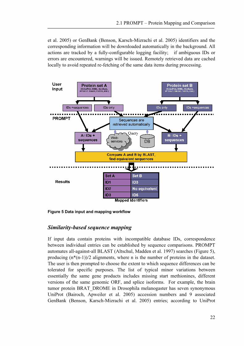
FASTA x x GenBank x x x EMBL x x Swiss-Prot x x x x x UniProt XML x x x x x Generic XML x x x Tab-delimited x x x WEKA x x Sequences and annotation available in major public databases may be fetched by their identifiers via the SeqHound (Michalickova, Bader et al. 2002) web services (Figure 5). All the user needs to do is to supply a list of UniProt (Bairoch, Apweiler
2.1 PROMPT – Protein Mapping and Comparison
22
et al. 2005) or GenBank (Benson, Karsch-Mizrachi et al. 2005) identifiers and the corresponding information will be downloaded automatically in the background. All actions are tracked by a fully-configurable logging facility; if ambiguous IDs or errors are encountered, warnings will be issued. Remotely retrieved data are cached locally to avoid repeated re-fetching of the same data items during processing.
Figure 5 Data input and mapping workflow
Similarity-based sequence mapping
If input data contain proteins with incompatible database IDs, correspondence between individual entries can be established by sequence comparisons. PROMPT automates all-against-all BLAST (Altschul, Madden et al. 1997) searches (Figure 5), producing (n*(n-1))/2 alignments, where n is the number of proteins in the dataset. The user is then prompted to choose the extent to which sequence differences can be tolerated for specific purposes. The list of typical minor variations between essentially the same gene products includes missing start methionines, different versions of the same genomic ORF, and splice isoforms. For example, the brain tumor protein BRAT_DROME in Drosophila melanogaster has seven synonymous UniProt (Bairoch, Apweiler et al. 2005) accession numbers and 9 associated GenBank (Benson, Karsch-Mizrachi et al. 2005) entries; according to UniProt
2.1 PROMPT – Protein Mapping and Comparison
23
(Bairoch, Apweiler et al. 2005) its amino acid sequence has been revised after the primary submission. Using the mechanism described above, a given list of GenBank (Benson, Karsch-Mizrachi et al. 2005) identifiers can be instantly mapped onto UniProt (Bairoch, Apweiler et al. 2005) accession numbers, PEDANT (Frishman, Albermann et al. 2001) protein codes, or EMBL (Cochrane, Aldebert et al. 2006) IDs. The PROMPT software facilitates adding new input data types to the mapping procedure by providing an interface for custom input adapters written in Java.
Computable sequence features
In addition to annotation features contained in input files a number of selected characteristics can be calculated directly from protein sequences, mainly using BioJava (Castillo-Davis and Hartl 2003). These include isoelectric point, the distance of the isoelectric point from neutrality, molecular weight in Daltons, sequence length, grand average hydrophobicity (GRAVY) and the total hydrophobicity of all residues. Additionally the number of alternating hydrophobic/ hydrophilic strands is calculated as described in Wong et al. (Wong, Fritz et al. 2005). We will be gradually adding additional computable sequence properties driven by our own research needs as well as user requests.
Statistical analyses
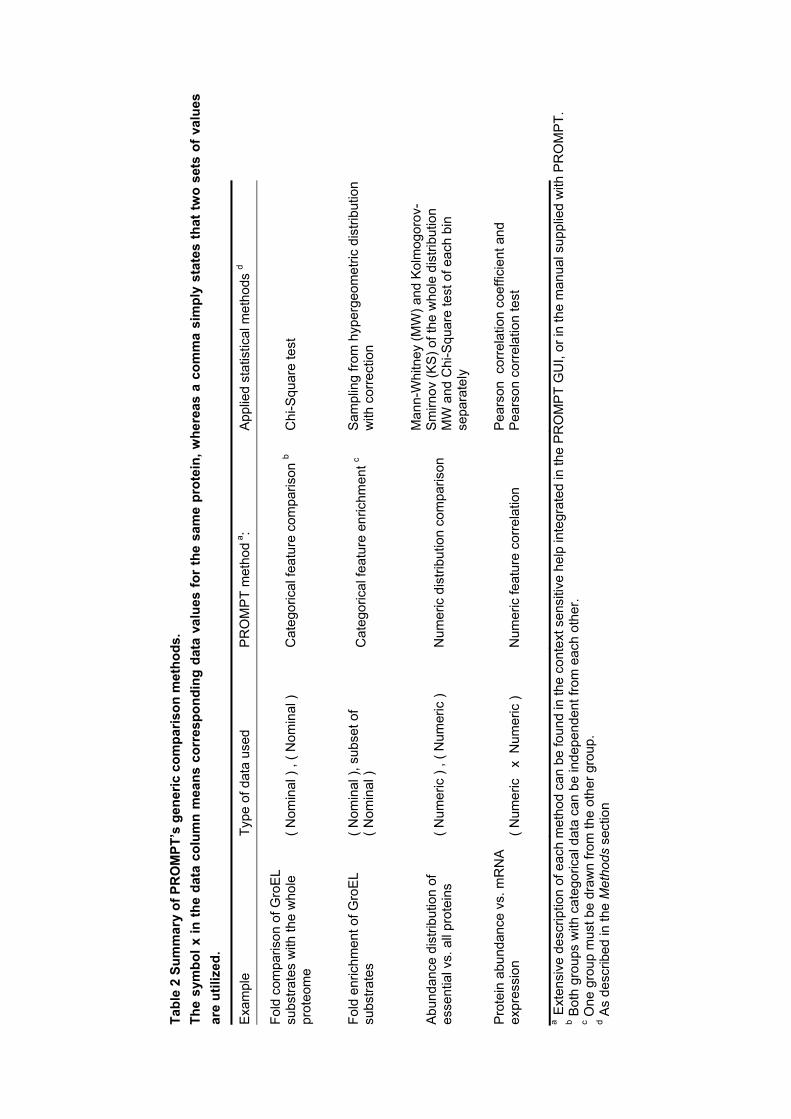
Formally, we are addressing the task of comparing two (protein) datasets in the space of N supplied features. PROMPT contains a set of generic engines to analyze and compare nominal as well as numerical attributes. In addition to generating basic descriptive statistics such as mean, standard deviation and median for the distribution of each feature, statistical tests are performed to determine whether the input sets differ significantly with respect to a feature of interest. All statistical tests are encapsulated as Java classes and predominantly use the free open source statistical software R or its commercial counterpart S-PLUS as reliable calculation engines. The linkage to R/S is accomplished by PROMPT automatically, assuming R/S is installed in default locations. Alternative and detailed R/S configuration settings can be provided by the user via the GUI configuration dialog, the XML configuration file, environmental parameters or by direct API usage. Although all tests can be chosen manually, PROMPT typically applies the appropriate tests automatically depending on the user’s type of input and addressed question. Basically, PROMPT distinguishes four different generic cases: i) comparison of the frequencies of categorical annotations between two sets, ii) enrichment of nominal features in one set with respect to another one, iii) comparison of numeric distributions, and iv) correlation of numeric variables. These four types of analyses are described in more detail below and are also exemplified in Table 2.
Tabl
e 2
Sum
mar
y of
PR
OM
PT’s
gen
eric
com
paris
on m
etho
ds.
The
sym
bol x
in th
e da
ta c
olum
n m
eans
cor
resp
ondi
ng d
ata
valu
es fo
r th
e sa
me
prot
ein,
whe
reas
a c
omm
a si
mpl
y st
ates
that
two
sets
of v
alue
s ar
e ut
ilize
d.
Exa
mpl
e Ty
pe o
f dat
a us
ed
PR
OM
PT
met
hod a
: A
pplie
d st
atis
tical
met
hods
d
Fold
com
paris
on o
f Gro
EL
subs
trate
s w
ith th
e w
hole
pr
oteo
me
( Nom
inal
) , (
Nom
inal
) C
ateg
oric
al fe
atur
e co
mpa
rison
b C
hi-S
quar
e te
st
Fold
enr
ichm
ent o
f Gro
EL
subs
trate
s ( N
omin
al ),
sub
set o
f ( N
omin
al )
Cat
egor
ical
feat
ure
enric
hmen
t c S
ampl
ing
from
hyp
erge
omet
ric d
istri
butio
n w
ith c
orre
ctio
n
Abu
ndan
ce d
istri
butio
n of
es
sent
ial v
s. a
ll pr
otei
ns
( Num
eric
) , (
Num
eric
) N
umer
ic d
istri
butio
n co
mpa
rison
Man
n-W
hitn
ey (M
W) a
nd K
olm
ogor
ov-
Sm
irnov
(KS
) of t
he w
hole
dis
tribu
tion
MW
and
Chi
-Squ
are
test
of e
ach
bin
sepa
rate
ly
Pro
tein
abu
ndan
ce v
s. m
RN
A
expr
essi
on
( N
umer
ic
x N
umer
ic )
Num
eric
feat
ure
corr
elat
ion
Pea
rson
cor
rela
tion
coef
ficie
nt a
nd
Pea
rson
cor
rela
tion
test
a E
xten
sive
des
crip
tion
of e
ach
met
hod
can
be fo
und
in th
e co
ntex
t sen
sitiv
e he
lp in
tegr
ated
in th
e P
RO
MP
T G
UI,
or in
the
man
ual s
uppl
ied
with
PR
OM
PT.
b B
oth
grou
ps w
ith c
ateg
oric
al d
ata
can
be in
depe
nden
t fro
m e
ach
othe
r. c O
ne g
roup
mus
t be
draw
n fro
m th
e ot
her g
roup
. d A
s de
scrib
ed in
the
Met
hods
sec
tion
2.1 PROMPT – Protein Mapping and Comparison
25
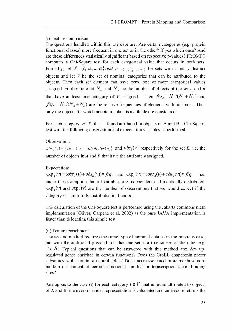
(i) Feature comparison The questions handled within this use case are: Are certain categories (e.g. protein functional classes) more frequent in one set or in the other? If yes which ones? And are these differences statistically significant based on respective p-values? PROMPT computes a Chi-Square test for each categorical value that occurs in both sets. Formally, let 1 2{ , ,..., }iA a a a= and 1 2{ , , ..., }jB b b b= be sets with i and j distinct objects and let V be the set of nominal categories that can be attributed to the objects. Then each set element can have zero, one or more categorical values assigned. Furthermore let aN and bN be the number of objects of the set A and B
that have at least one category of V assigned. Then /( )A A A Bfrq N N N= + and /( )B B A Bfrq N N N= + are the relative frequencies of elements with attributes. Thus
only the objects for which annotation data is available are considered. For each category v V∈ that is found attributed to objects of A and B a Chi-Square test with the following observation and expectation variables is performed: Observation:
{ }( ) | ( )aobs v a A v attributes a= ∈ ∈ and ( )bobs v respectively for the set B, i.e. the
number of objects in A and B that have the attribute v assigned. Expectation: exp ( ) ( ( ) ( ))A A B Av obs v obs v frq= + ∗ and exp ( ) ( ( ) ( ))B A B Bv obs v obs v frq= + ∗ , i.e. under the assumption that all variables are independent and identically distributed, exp ( )A v and exp ( )B v are the number of observations that we would expect if the category v is uniformly distributed in A and B. The calculation of the Chi-Square test is performed using the Jakarta commons math implementation (Oliver, Carpena et al. 2002) as the pure JAVA implementation is faster than delegating this simple test. (ii) Feature enrichment The second method requires the same type of nominal data as in the previous case, but with the additional precondition that one set is a true subset of the other e.g. A B⊂ . Typical questions that can be answered with this method are: Are up-regulated genes enriched in certain functions? Does the GroEL chaperonin prefer substrates with certain structural folds? Do cancer-associated proteins show non-random enrichment of certain functional families or transcription factor binding sites? Analogous to the case (i) for each category v V∈ that is found attributed to objects of A and B, the over- or under representation is calculated and an e-score returns the
2.1 PROMPT – Protein Mapping and Comparison
26
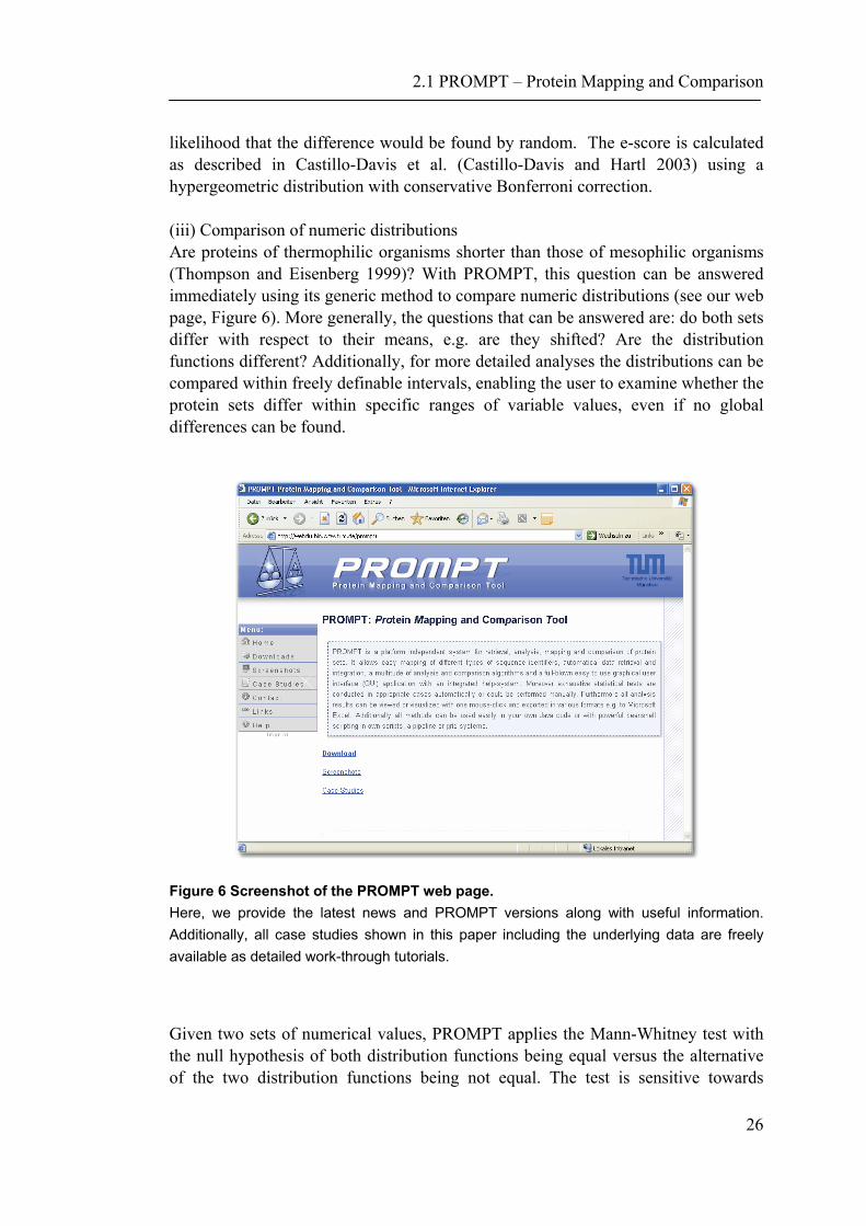
likelihood that the difference would be found by random. The e-score is calculated as described in Castillo-Davis et al. (Castillo-Davis and Hartl 2003) using a hypergeometric distribution with conservative Bonferroni correction. (iii) Comparison of numeric distributions Are proteins of thermophilic organisms shorter than those of mesophilic organisms (Thompson and Eisenberg 1999)? With PROMPT, this question can be answered immediately using its generic method to compare numeric distributions (see our web page, Figure 6). More generally, the questions that can be answered are: do both sets differ with respect to their means, e.g. are they shifted? Are the distribution functions different? Additionally, for more detailed analyses the distributions can be compared within freely definable intervals, enabling the user to examine whether the protein sets differ within specific ranges of variable values, even if no global differences can be found.
Figure 6 Screenshot of the PROMPT web page. Here, we provide the latest news and PROMPT versions along with useful information. Additionally, all case studies shown in this paper including the underlying data are freely available as detailed work-through tutorials.
Given two sets of numerical values, PROMPT applies the Mann-Whitney test with the null hypothesis of both distribution functions being equal versus the alternative of the two distribution functions being not equal. The test is sensitive towards
2.1 PROMPT – Protein Mapping and Comparison
27
differences in the mean, but not towards different variances. Given a continuous distribution function, the two-sample Kolmogorov-Smirnov test checks the null hypothesis that both variables are equally distributed. Both tests can only be applied under the assumption of the variables being independent. They have the advantage that they do not assume the data to follow any specific statistical distribution. By providing the Mann-Whitney and the Kolomogorov-Smirnov test, PROMPT covers both discrete and continuous input data. For both datasets the key statistical values (such as minimum, maximum, mean, median and standard deviation) as well as histograms with equal binning are calculated. The relative difference of observed values is computed and its significance tested by a Chi-Square test. The Mann-Whitney test is applied to the values of all histogram intervals in order to test whether the distribution functions of the two datasets are identical within each bin. (iv) Correlation of numeric variables PROMPT provides a generic method to check for correlation between two numeric variables. First, the Pearson correlation coefficient is calculated which is not based on any assumptions about the variables’ distributions. Secondly, the Pearson correlation test is performed which expects samples from two independent, bivariate normally distributed distributions. The null hypothesis is that no correlation either negative or positive exists.
Graphical user interface and scripting capabilities
All implemented algorithms can be comfortably run via a stand-alone application with a graphical user interface (GUI), as well as from custom scripts or JAVA programs. The GUI provides a dynamical workspace where input data and results can be managed, analyses performed, statistical tests executed and the results examined, visualized or further processed (Figure 7). All available input adapters, statistical tests and algorithms can be accessed through a menu bar. The menu bar and the GUI itself are fully configurable and extensible by new in-house or third-party modules through XML configuration files or configuration dialogs. The GUI workspace allows confident handling of multiple data sources, analyses, and results, and supports saving and loading any of the input or result objects to/from files. Moreover, the entire workspace can be stored in a compressed form and restored later so that the work on a particular project can be suspended and resumed by the user at any time. The workspace files are portable and can be transferred to other computer systems and shared between different users.
2.1 PROMPT – Protein Mapping and Comparison
28
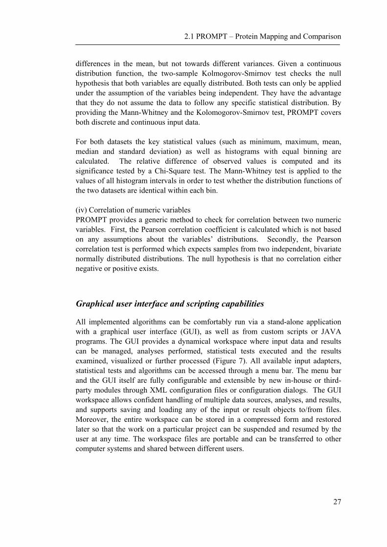
Figure 7 Graphical User Interface (GUI). Shown is a typical workspace session with input data and results. The information panel in the bottom part of the screen provides context sensitive information related to the current user action.
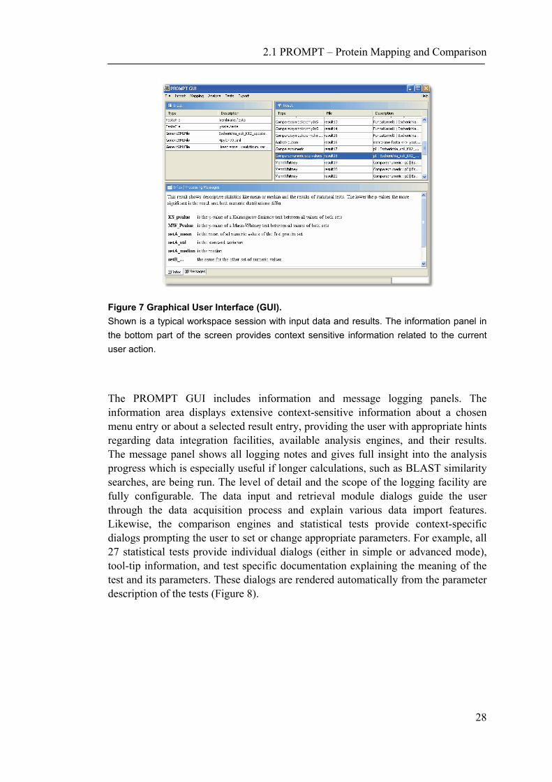
The PROMPT GUI includes information and message logging panels. The information area displays extensive context-sensitive information about a chosen menu entry or about a selected result entry, providing the user with appropriate hints regarding data integration facilities, available analysis engines, and their results. The message panel shows all logging notes and gives full insight into the analysis progress which is especially useful if longer calculations, such as BLAST similarity searches, are being run. The level of detail and the scope of the logging facility are fully configurable. The data input and retrieval module dialogs guide the user through the data acquisition process and explain various data import features. Likewise, the comparison engines and statistical tests provide context-specific dialogs prompting the user to set or change appropriate parameters. For example, all 27 statistical tests provide individual dialogs (either in simple or advanced mode), tool-tip information, and test specific documentation explaining the meaning of the test and its parameters. These dialogs are rendered automatically from the parameter description of the tests (Figure 8).
2.1 PROMPT – Protein Mapping and Comparison
29
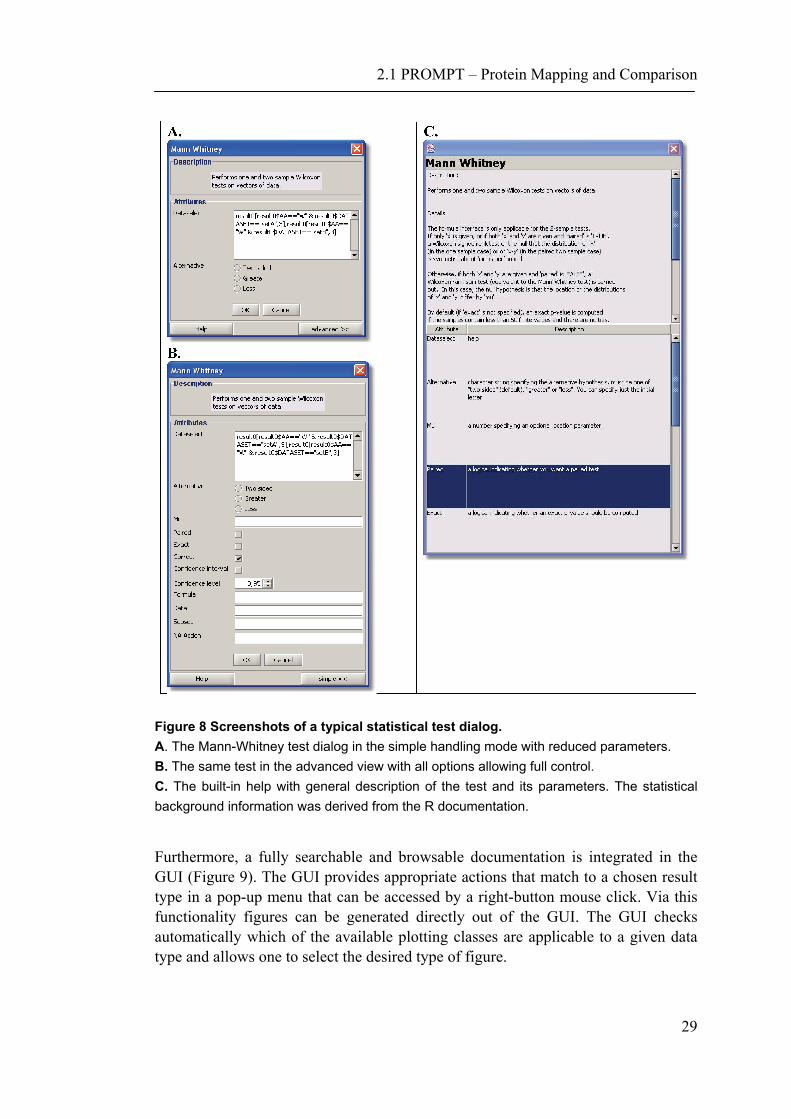
Figure 8 Screenshots of a typical statistical test dialog. A. The Mann-Whitney test dialog in the simple handling mode with reduced parameters. B. The same test in the advanced view with all options allowing full control. C. The built-in help with general description of the test and its parameters. The statistical background information was derived from the R documentation.
Furthermore, a fully searchable and browsable documentation is integrated in the GUI (Figure 9). The GUI provides appropriate actions that match to a chosen result type in a pop-up menu that can be accessed by a right-button mouse click. Via this functionality figures can be generated directly out of the GUI. The GUI checks automatically which of the available plotting classes are applicable to a given data type and allows one to select the desired type of figure.
2.1 PROMPT – Protein Mapping and Comparison
30
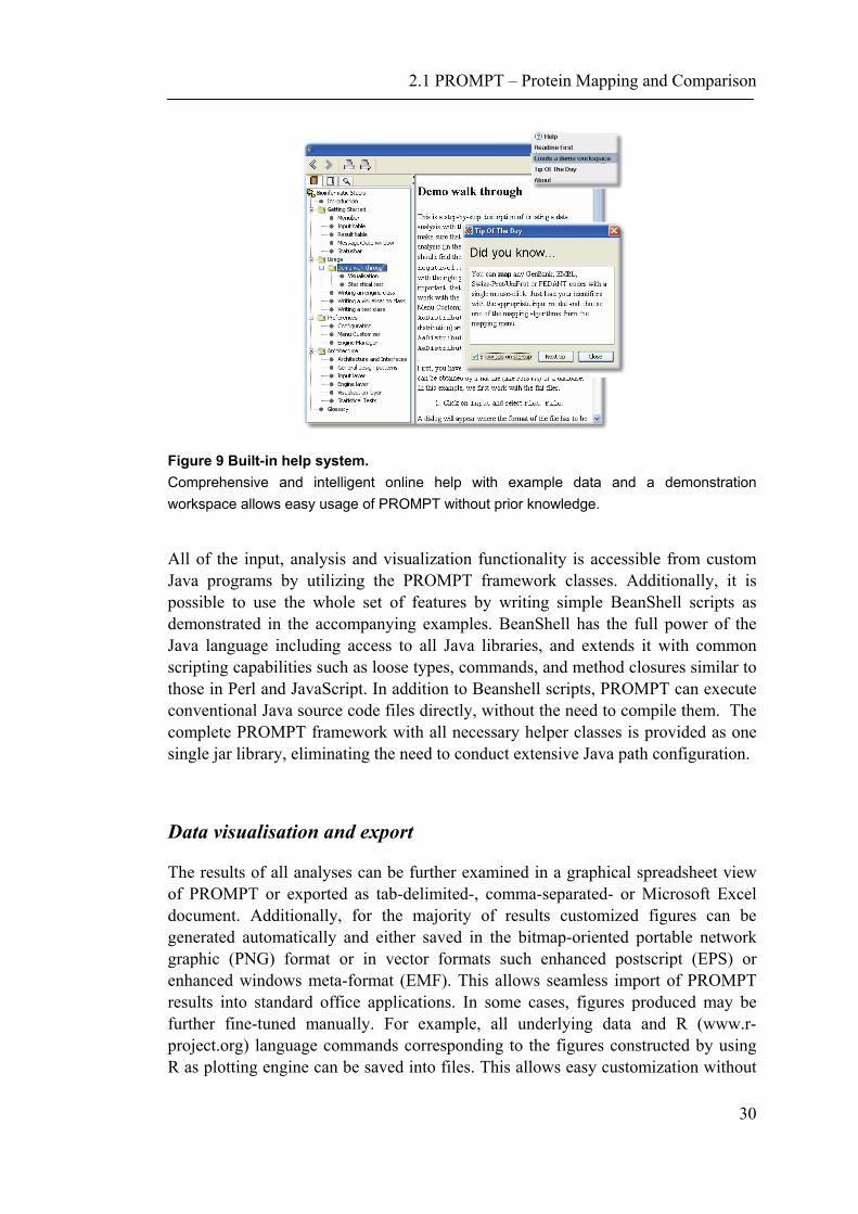
Figure 9 Built-in help system. Comprehensive and intelligent online help with example data and a demonstration workspace allows easy usage of PROMPT without prior knowledge.
All of the input, analysis and visualization functionality is accessible from custom Java programs by utilizing the PROMPT framework classes. Additionally, it is possible to use the whole set of features by writing simple BeanShell scripts as demonstrated in the accompanying examples. BeanShell has the full power of the Java language including access to all Java libraries, and extends it with common scripting capabilities such as loose types, commands, and method closures similar to those in Perl and JavaScript. In addition to Beanshell scripts, PROMPT can execute conventional Java source code files directly, without the need to compile them. The complete PROMPT framework with all necessary helper classes is provided as one single jar library, eliminating the need to conduct extensive Java path configuration.
Data visualisation and export
The results of all analyses can be further examined in a graphical spreadsheet view of PROMPT or exported as tab-delimited-, comma-separated- or Microsoft Excel document. Additionally, for the majority of results customized figures can be generated automatically and either saved in the bitmap-oriented portable network graphic (PNG) format or in vector formats such enhanced postscript (EPS) or enhanced windows meta-format (EMF). This allows seamless import of PROMPT results into standard office applications. In some cases, figures produced may be further fine-tuned manually. For example, all underlying data and R (www.r-project.org) language commands corresponding to the figures constructed by using R as plotting engine can be saved into files. This allows easy customization without
2.1 PROMPT – Protein Mapping and Comparison
31
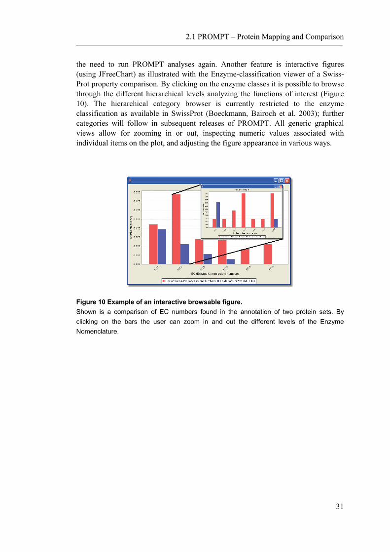
the need to run PROMPT analyses again. Another feature is interactive figures (using JFreeChart) as illustrated with the Enzyme-classification viewer of a Swiss-Prot property comparison. By clicking on the enzyme classes it is possible to browse through the different hierarchical levels analyzing the functions of interest (Figure 10). The hierarchical category browser is currently restricted to the enzyme classification as available in SwissProt (Boeckmann, Bairoch et al. 2003); further categories will follow in subsequent releases of PROMPT. All generic graphical views allow for zooming in or out, inspecting numeric values associated with individual items on the plot, and adjusting the figure appearance in various ways.
Figure 10 Example of an interactive browsable figure. Shown is a comparison of EC numbers found in the annotation of two protein sets. By clicking on the bars the user can zoom in and out the different levels of the Enzyme Nomenclature.
2.1 PROMPT – Protein Mapping and Comparison
32
2.1.3 Applications
Here, we demonstrate the functionality of PROMPT based on three well documented test cases. Each case study highlights different elementary analysis modes of PROMPT. All used data can be found on the PROMPT home page (Figure 6), where we additionally provide detailed step-by-step instructions for all cases along with up-to-date information.
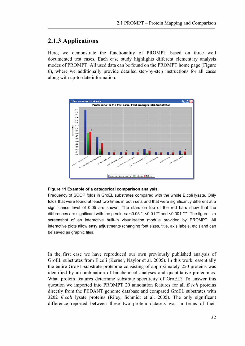
Figure 11 Example of a categorical comparison analysis. Frequency of SCOP folds in GroEL substrates compared with the whole E.coli lysate. Only folds that were found at least two times in both sets and that were significantly different at a significance level of 0.05 are shown. The stars on top of the red bars show that the differences are significant with the p-values: <0.05 *, <0.01 ** and <0.001 ***. The figure is a screenshot of an interactive built-in visualisation module provided by PROMPT. All interactive plots allow easy adjustments (changing font sizes, title, axis labels, etc.) and can be saved as graphic files.
In the first case we have reproduced our own previously published analysis of GroEL substrates from E.coli (Kerner, Naylor et al. 2005). In this work, essentially the entire GroEL-substrate proteome consisting of approximately 250 proteins was identified by a combination of biochemical analyses and quantitative proteomics. What protein features determine substrate specificity of GroEL? To answer this question we imported into PROMPT 20 annotation features for all E.coli proteins directly from the PEDANT genome database and compared GroEL substrates with 3202 E.coli lysate proteins (Riley, Schmidt et al. 2005). The only significant difference reported between these two protein datasets was in terms of their
2.1 PROMPT – Protein Mapping and Comparison
33
structural folds. Using PROMPT’s nominal comparison method we could easily demonstrate that the GroEL substrates are significantly enriched in proteins possessing the TIM-barrel fold (Figure 11). Possible evolutionary implications of this phenomenon are discussed in Kerner et al. (Kerner, Naylor et al. 2005). Thus, PROMPT allows finding significant enrichments and differences of categorical features between two sets of elements. Furthermore, the generic solution allows an analysis independent of the feature semantic and problem domain.
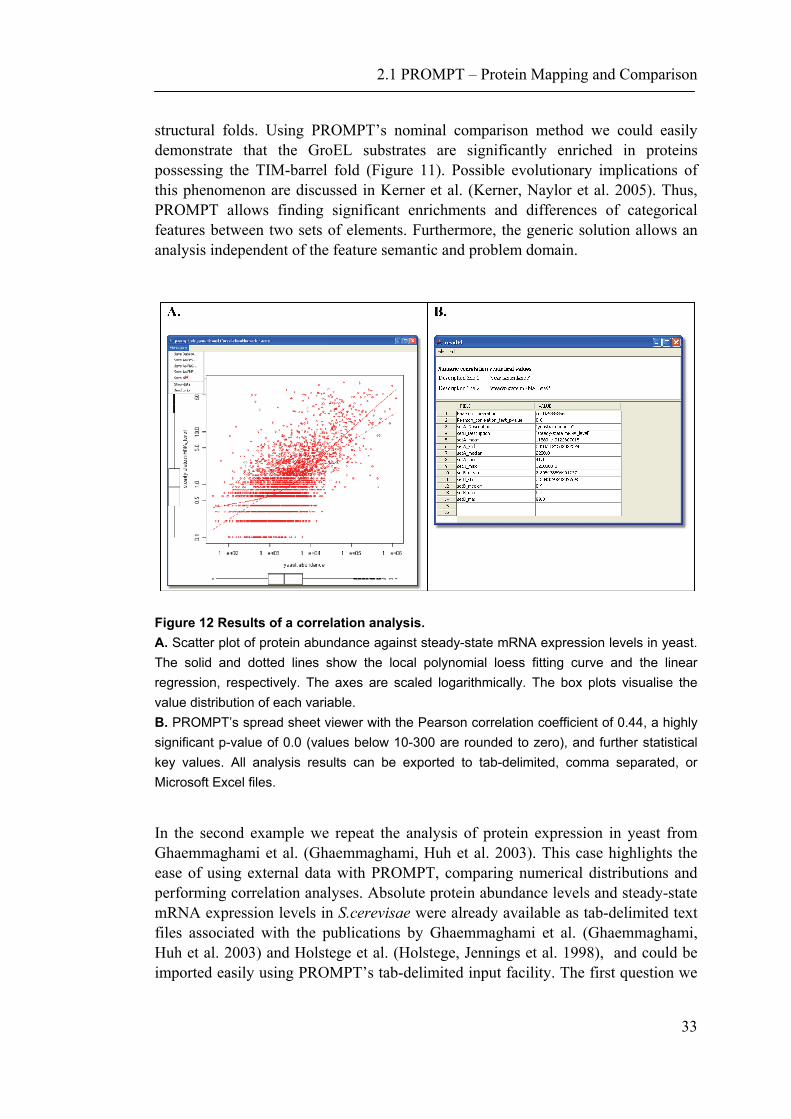
Figure 12 Results of a correlation analysis. A. Scatter plot of protein abundance against steady-state mRNA expression levels in yeast. The solid and dotted lines show the local polynomial loess fitting curve and the linear regression, respectively. The axes are scaled logarithmically. The box plots visualise the value distribution of each variable. B. PROMPT’s spread sheet viewer with the Pearson correlation coefficient of 0.44, a highly significant p-value of 0.0 (values below 10-300 are rounded to zero), and further statistical key values. All analysis results can be exported to tab-delimited, comma separated, or Microsoft Excel files.
In the second example we repeat the analysis of protein expression in yeast from Ghaemmaghami et al. (Ghaemmaghami, Huh et al. 2003). This case highlights the ease of using external data with PROMPT, comparing numerical distributions and performing correlation analyses. Absolute protein abundance levels and steady-state mRNA expression levels in S.cerevisae were already available as tab-delimited text files associated with the publications by Ghaemmaghami et al. (Ghaemmaghami, Huh et al. 2003) and Holstege et al. (Holstege, Jennings et al. 1998), and could be imported easily using PROMPT’s tab-delimited input facility. The first question we
2.1 PROMPT – Protein Mapping and Comparison
34
addressed was whether protein abundance correlates with mRNA expression levels. In addition to calculating the Pearson correlation coefficient PROMPT assesses its statistical significance by performing a correlation test. For visualization of results PROMPT will suggest appropriate options which in this case include a static scatter plot of abundance versus mRNA levels with logarithmic axes and linear- as well as polynomial loess regression lines. Besides the statistical test results, descriptive key data such as minimum, maximum, mean, median and standard deviation are always returned by PROMPT and can be analysed, sorted and further processed within a comfortable spread sheet viewer as seen in Figure 12.
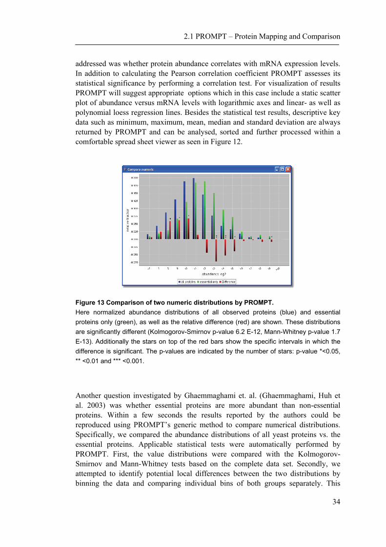
Figure 13 Comparison of two numeric distributions by PROMPT. Here normalized abundance distributions of all observed proteins (blue) and essential proteins only (green), as well as the relative difference (red) are shown. These distributions are significantly different (Kolmogorov-Smirnov p-value 6.2 E-12, Mann-Whitney p-value 1.7 E-13). Additionally the stars on top of the red bars show the specific intervals in which the difference is significant. The p-values are indicated by the number of stars: p-value *<0.05, ** <0.01 and *** <0.001.
Another question investigated by Ghaemmaghami et. al. (Ghaemmaghami, Huh et al. 2003) was whether essential proteins are more abundant than non-essential proteins. Within a few seconds the results reported by the authors could be reproduced using PROMPT’s generic method to compare numerical distributions. Specifically, we compared the abundance distributions of all yeast proteins vs. the essential proteins. Applicable statistical tests were automatically performed by PROMPT. First, the value distributions were compared with the Kolmogorov-Smirnov and Mann-Whitney tests based on the complete data set. Secondly, we attempted to identify potential local differences between the two distributions by binning the data and comparing individual bins of both groups separately. This

2.1 PROMPT – Protein Mapping and Comparison
35
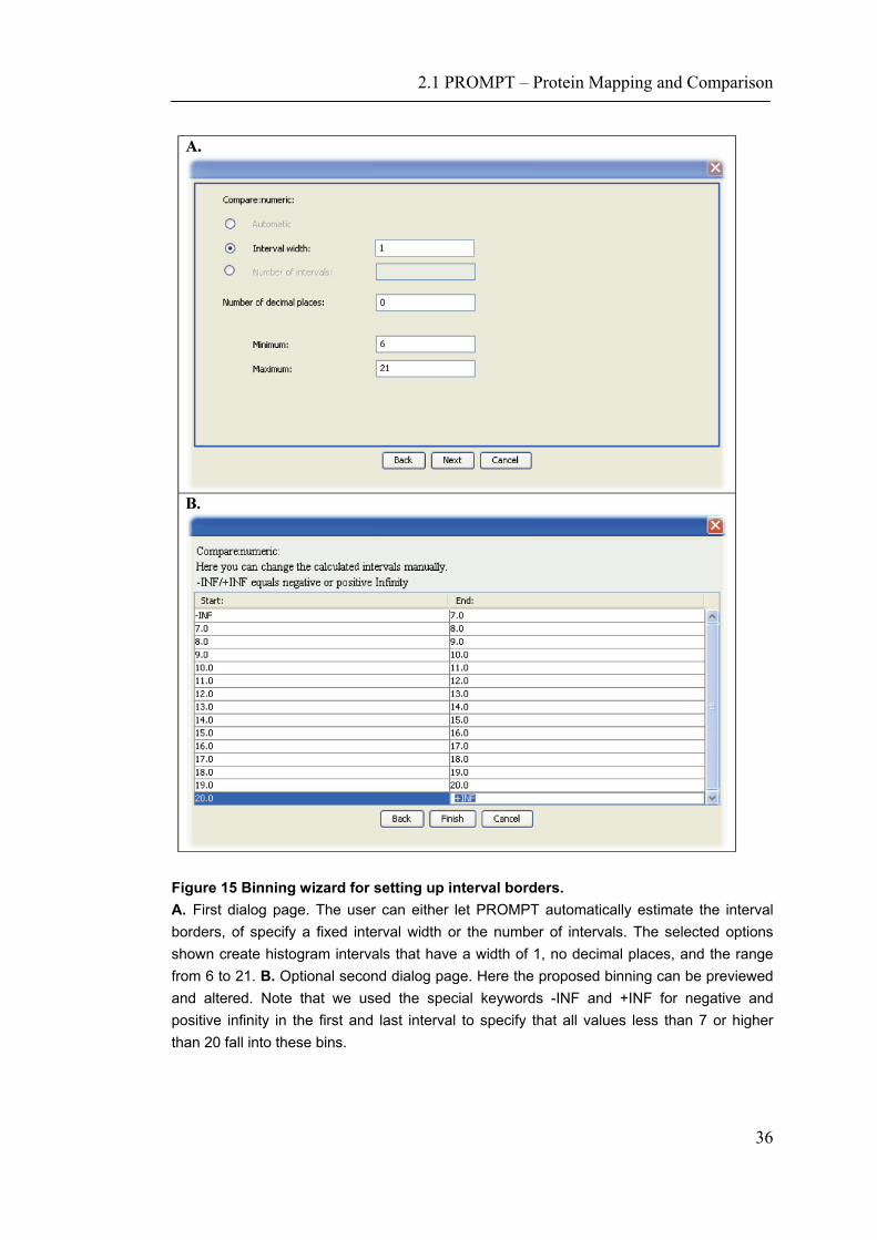
demonstrates that essential proteins are significantly underrepresented within the logarithmic abundance ranges 8 to 11 and significantly overrepresented within the range 13 to 16. The bin intervals can be chosen either automatically or manually guided by a user-friendly graphical dialog box (Figure 15). The resulting comparison of the protein abundance levels of essential proteins versus the complete yeast proteome is shown in Figure 13.
A B
Figure 14 Examples of built-in interactive plots. A. Screenshot of a scatterplot. Protein length of E.coli lysate proteins is plotted against their hydrophobicity. The Pearson correlation coefficient is -0.69 with a p-value of 2.8E-54. By pressing and holding the left mouse button it is possible to zoom in the desired area. Clicking on an individual point on the plot leads to numeric values associated with this point being displayed. B. Usage of derived sequence based properties in a generic analysis of PROMPT. Here the isoelectric point (pI) distributions of the E.coli lysate and membrane proteins are compared using the numeric comparison method. PROMPT calculates the pI values automatically if protein sequences are available.
2.1 PROMPT – Protein Mapping and Comparison
36
Figure 15 Binning wizard for setting up interval borders. A. First dialog page. The user can either let PROMPT automatically estimate the interval borders, of specify a fixed interval width or the number of intervals. The selected options shown create histogram intervals that have a width of 1, no decimal places, and the range from 6 to 21. B. Optional second dialog page. Here the proposed binning can be previewed and altered. Note that we used the special keywords -INF and +INF for negative and positive infinity in the first and last interval to specify that all values less than 7 or higher than 20 fall into these bins.
2.1 PROMPT – Protein Mapping and Comparison
37
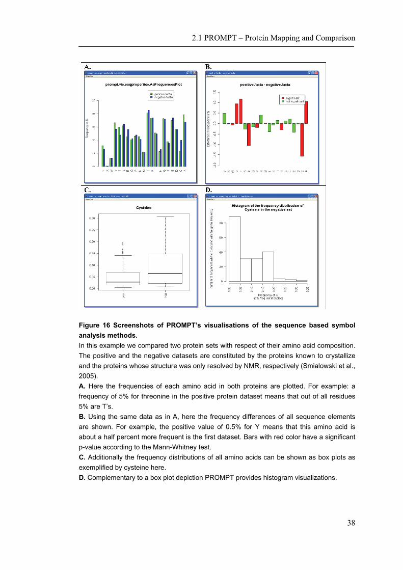
In the final example we use PROMPT to automatically retrieve protein sequences by sequence identifiers from public databases and to calculate some of their basic properties such as the isoelectric point. As input we used two lists of GenBank (Benson, Karsch-Mizrachi et al. 2005) identifiers of membrane and globular proteins of E.coli. In this experiment we use only multi-spanning membrane proteins with more than 6 membrane spanning regions predicted by TMHMM 2.0 (Krogh, Larsson et al. 2001) to avoid any noise from false positive predictions or small membrane-coupled proteins. As seen in Figure 14 A, longer membrane proteins are less hydrophobic than shorter ones. The observed high correlation between the protein length and its hydrophobicity (expressed as the GRAVY index) of -0.7 is significant with a p-value of 3 E-54. Sequence based properties can also be used in any other generic analysis. For example, Figure 14 B shows a comparison of the automatically derived pI values of membrane and lysate proteins. In addition to the methods based on amino acid sequences, PROMPT provides statistical analyses and comparisons of symbol frequencies of arbitrary alphabets. Thus, in addition to finding over- or under-represented amino acids in a given protein dataset (Figure 16), it is also possible to calculate the enrichment/depletion of other symbols such as those taken from the three-state secondary structure alphabet with Helix (H), Strand (E) and Coil (C) as elements.
2.1 PROMPT – Protein Mapping and Comparison
38
Figure 16 Screenshots of PROMPT’s visualisations of the sequence based symbol analysis methods. In this example we compared two protein sets with respect of their amino acid composition. The positive and the negative datasets are constituted by the proteins known to crystallize and the proteins whose structure was only resolved by NMR, respectively (Smialowski et al., 2005). A. Here the frequencies of each amino acid in both proteins are plotted. For example: a frequency of 5% for threonine in the positive protein dataset means that out of all residues 5% are T’s. B. Using the same data as in A, here the frequency differences of all sequence elements are shown. For example, the positive value of 0.5% for Y means that this amino acid is about a half percent more frequent is the first dataset. Bars with red color have a significant p-value according to the Mann-Whitney test. C. Additionally the frequency distributions of all amino acids can be shown as box plots as exemplified by cysteine here. D. Complementary to a box plot depiction PROMPT provides histogram visualizations.
2.1 PROMPT – Protein Mapping and Comparison
39
2.1.4 Discussion
PROMPT is a platform-independent, multi-purpose stand-alone software system for solving a broad spectrum of standard problems in comparative proteomics. It is implemented as a highly-reusable and extensible framework for analysing biological data. With its rich data integration functionality and built-in statistical tests, PROMPT facilitates data mining and hypothesis testing. PROMPT makes possible incorporation of new algorithms by providing hulls, layers and infrastructure. The availability of both scripting-capability and an intuitive GUI with a context-sensitive help system makes PROMPT equally accessible to both professional bioinformaticians and biologically oriented users. The structure of PROMPT is well adapted for batch processing and automation. Unlike the multitude of specialized analytical tools, PROMPT has been designed as a versatile general platform for routine analyses and comparisons in the field of molecular bioinformatics. The current version of PROMPT includes a large set of generic comparison methods and statistical tests applicable to any nominal and numeric data as shown in Table 2. User-specific extensions and custom methods can be seamlessly integrated by providing Java classes that implement the interfaces defined in the PROMPT documentation and by adding additional entries to the application’s configuration file. Although PROMPT is easily extensible by third-parties, we encourage members of the scientific community to suggest new PROMPT features that may be of particular interest to their research. In the long run we hope to make PROMPT a community resource for comparative proteomics (Schmidt and Frishman 2006).
2.2 Integration of functional and physical annotations
40
2.2 Integration of functional and physical annotations
A major challenge towards a comprehensive analysis of biological systems is the integration of data from different “omics” sources and their interpretation at a functional level. Here we address this issue by analysing transcriptomic and proteomic datasets from mouse brain tissue at embryonic days 9.5 and 13.5 provided from (Daniela Hartl). In the following, we give an example how the PROMPT software suite for comparative proteomics is suited to analyse physical features of regulated gene products from multiple databases. This application demonstrate PROMPT’s advantages in integration- and data analysis of experimental expression data (Irmler, Hartl et al. 2008).
2.2.1 Introduction
Since the advent of high-throughput techniques to study gene expression at transcriptome and proteome levels, large datasets are being generated. Generally these datasets are analyzed by distinct tools, each developed for the individual datasets (Meunier, Bouley et al. 2005; Rainer, Sanchez-Cabo et al. 2006; Meunier, Dumas et al. 2007). However, transcriptome and proteome feedback to each other in a highly complex and controlled manner and should therefore be analyzed by integrative approaches. The inclusion of information derived from other resources such as public databases would assist the functional interpretation of expression data and provide a basis for the emerging field of systems biology. However, there is an apparent lack of tools to translate the information from various sources and levels into a common processible format (Hack 2004). Also, standardized methodologies for data analysis, for example for the correct assignment of transcripts to their corresponding proteins, are needed, to allow better comparability of results. Such methods are being developed (Cox, Kislinger et al. 2005; Cox, Kislinger et al. 2007) and make use of hierarchical clustering methods combined with statistical analysis of large datasets. In a recent study, the developing mouse brain at embryonic days 9.5 and 13.5 (E9.5 and E13.5) was analyzed (Daniela Hartl). During these two days the brain undergoes major morphological changes and differentiation processes. Due to these cellular differentiation and patterning processes a high number of genes and proteins undergo changes in expression levels providing a sufficient amount of data for statistical analysis. Here we provide an example of how the PROMPT tool (Schmidt and Frishman 2006) can add to the functional interpretation of such an analysis.
2.2 Integration of functional and physical annotations
41
2.2.2 Material and Methods
Data
The transcriptome and proteome data in this experiment was obtained from (Daniela Hartl). Briefly, for transcript analyses whole genome Affymetrix MOE430 2.0 arrays were used with 45k probe sets. The proteome dataset was derived from 2-dimensional fluorescence difference gel electrophoresis (DIGE). Of about 3,700 distinct protein spots detectable in each gel, 300 spots were identified by mass spectrometry. About 15 % of all transcripts present on the array and 30 % of all DIGE-detectable proteins were significantly regulated between both developmental stages. The resulting gene and protein lists were used for further analysis in this work.
Properties
Functional roles of gene products were described in terms of the manually curated hierarchical functional catalogue (FunCat) developed at MIPS (Ruepp, Zollner et al. 2004). In this catalogue each of the 16 main classes (e.g., metabolism, energy) may contain up to six subclasses. An essential feature of FUNCAT is its multidimensionality, meaning that any protein can be assigned to multiple categories. Carefully verified FunCat assignment as well as enzyme classifications, InterPro domains (Mulder, Apweiler et al. 2002; Mulder, Apweiler et al. 2007) and genomic (e.g. number of exons) as well as sequence information was taken from the Mouse Functional Genome Database (MfunGD) (Ruepp, Doudieu et al. 2006). Gene Ontology (GO) functional annotations (Ashburner, Ball et al. 2000), Mammalian Phenotype (MP) classification (Smith, Goldsmith et al. 2005) and the currently known number of single nucleotide polymorphisms (SNPs) were obtained from The Mouse Genome Database (MGD) (Eppig, Bult et al. 2005) as of June 2007. Disorder, low complexity, probability to be non-globular or adopt a coiled-coiled structure, similarity to clusters of orthologous groups (COGs) (Tatusov, Koonin et al. 1997; Tatusov, Fedorova et al. 2003) and protein structural information were taken from our PEDANT database Mus_musculus_new (Frishman, Mokrejs et al. 2003; Riley, Schmidt et al. 2005; Riley, Schmidt et al. 2007). Disorder attributes were calculated with the software GlobPlot (Linding, Russell et al. 2003). GlobProt utilizes the statistics of proteins known to have unstructured regions (Wright and Dyson 1999; Tompa 2002). Low complexity and non-globular regions were computed with the original SEG algorithm (Wootton 1994). The probability that a protein structure adopts a coiled-coiled structure was calculated with the program COILS program (Lupas, Van Dyke et al. 1991). Protein structures were further
2.2 Integration of functional and physical annotations
42
analyzed with regard of their secondary structure content i.e. percentage of residues that are part of alpha helices, beta sheets or coils and their three dimensional structure folds using the SCOP classification schema. Like FunCat the SCOP database (Murzin, Brenner et al. 1995; Andreeva, Howorth et al. 2004) provides a hierarchical classification of protein structural domains. Data retrieval from PEDANT was accomplished using the protein mapping and comparison tool PROMPT version 0.9.2 (Schmidt and Frishman 2006). SCOP class and COG assignments to M. musculus proteins were based on BLAST (Altschul, Gish et al. 1990) hits with an E-value of 10-4 (PROMPT default thresholds). The number of alternating hydrophobic/hydrophilic stretches was computed as described (Wong, Fritz et al. 2005) using the implementation of PROMPT. The residues A, C, F, G, I, L, M, P, V, W and Y were considered to be hydrophobic and H, Q, N, S, T, K, R, D, E were considered hydrophilic in this thereby. The hydrophobicity of a protein was defined as average of the hydrophobicity values of the amino acids averaged over the complete protein. Hydrophobicity values were calculated using the Kyte-Doolittle scale (Kyte and Doolittle 1982). Molecular protein mass, theoretical isoelectric point (pI) as well the averaged hydrophobicity were calculated with the PROMPT software from the amino acid sequences.
Statistics
All statistical tests and most figures were done using the R software package version 2.5.0 (www.r-project.org) and PROMPT (Schmidt and Frishman 2006). To compare the distributions of two unpaired samples with non-Gaussian or unknown distributions, the rank-sum Mann-Whitney (MW) test and the two sample Kolmogorov-Smirnov (KS) were applied using the significance threshold α=0.05. Briefly spoken, the null hypothesis of the Mann-Whitney test is that the abundance means are equal; the null hypothesis of the Kolmogorov-Smirnov test is that the values of the two samples are drawn from the same continuous distributions. Both tests have the advantage that they make almost no assumptions about the distribution of data.
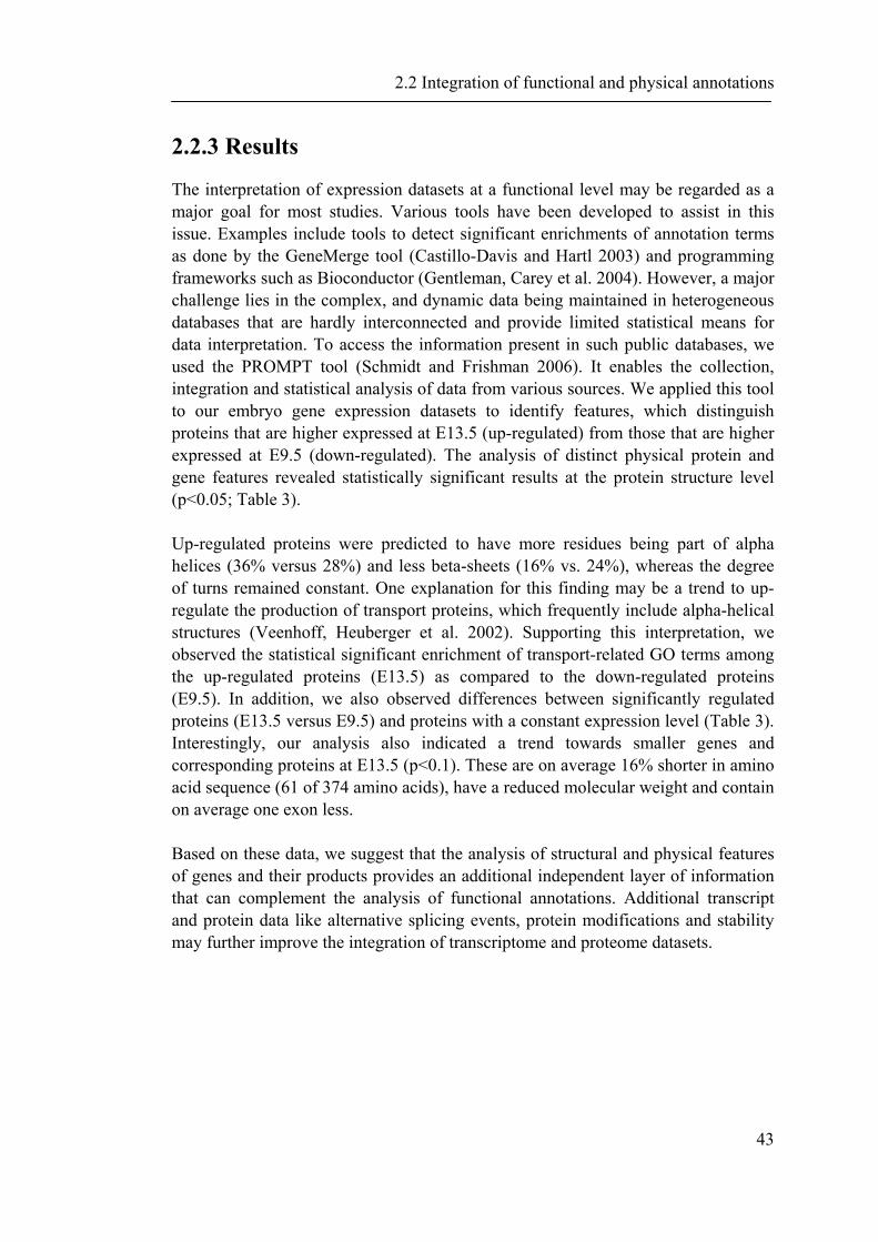
2.2 Integration of functional and physical annotations
43
2.2.3 Results
The interpretation of expression datasets at a functional level may be regarded as a major goal for most studies. Various tools have been developed to assist in this issue. Examples include tools to detect significant enrichments of annotation terms as done by the GeneMerge tool (Castillo-Davis and Hartl 2003) and programming frameworks such as Bioconductor (Gentleman, Carey et al. 2004). However, a major challenge lies in the complex, and dynamic data being maintained in heterogeneous databases that are hardly interconnected and provide limited statistical means for data interpretation. To access the information present in such public databases, we used the PROMPT tool (Schmidt and Frishman 2006). It enables the collection, integration and statistical analysis of data from various sources. We applied this tool to our embryo gene expression datasets to identify features, which distinguish proteins that are higher expressed at E13.5 (up-regulated) from those that are higher expressed at E9.5 (down-regulated). The analysis of distinct physical protein and gene features revealed statistically significant results at the protein structure level (p<0.05; Table 3). Up-regulated proteins were predicted to have more residues being part of alpha helices (36% versus 28%) and less beta-sheets (16% vs. 24%), whereas the degree of turns remained constant. One explanation for this finding may be a trend to up-regulate the production of transport proteins, which frequently include alpha-helical structures (Veenhoff, Heuberger et al. 2002). Supporting this interpretation, we observed the statistical significant enrichment of transport-related GO terms among the up-regulated proteins (E13.5) as compared to the down-regulated proteins (E9.5). In addition, we also observed differences between significantly regulated proteins (E13.5 versus E9.5) and proteins with a constant expression level (Table 3). Interestingly, our analysis also indicated a trend towards smaller genes and corresponding proteins at E13.5 (p<0.1). These are on average 16% shorter in amino acid sequence (61 of 374 amino acids), have a reduced molecular weight and contain on average one exon less. Based on these data, we suggest that the analysis of structural and physical features of genes and their products provides an additional independent layer of information that can complement the analysis of functional annotations. Additional transcript and protein data like alternative splicing events, protein modifications and stability may further improve the integration of transcriptome and proteome datasets.
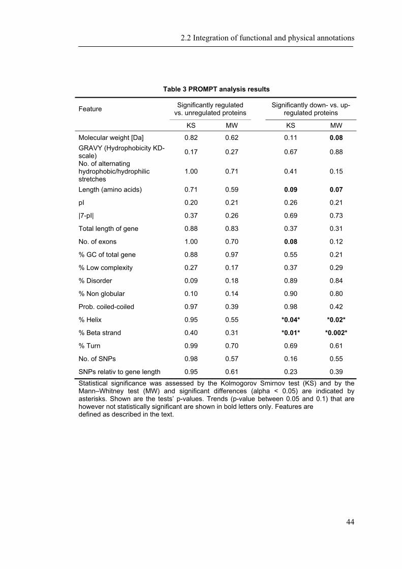
2.2 Integration of functional and physical annotations
44
Table 3 PROMPT analysis results
Feature Significantly regulated vs. unregulated proteins Significantly down- vs. up-
regulated proteins
KS MW KS MW
Molecular weight [Da] 0.82 0.62 0.11 0.08 GRAVY (Hydrophobicity KD-scale) 0.17 0.27 0.67 0.88
No. of alternating hydrophobic/hydrophilic stretches
1.00 0.71 0.41 0.15
Length (amino acids) 0.71 0.59 0.09 0.07
pI 0.20 0.21 0.26 0.21
|7-pI| 0.37 0.26 0.69 0.73
Total length of gene 0.88 0.83 0.37 0.31
No. of exons 1.00 0.70 0.08 0.12
% GC of total gene 0.88 0.97 0.55 0.21
% Low complexity 0.27 0.17 0.37 0.29
% Disorder 0.09 0.18 0.89 0.84
% Non globular 0.10 0.14 0.90 0.80
Prob. coiled-coiled 0.97 0.39 0.98 0.42
% Helix 0.95 0.55 *0.04* *0.02*
% Beta strand 0.40 0.31 *0.01* *0.002*
% Turn 0.99 0.70 0.69 0.61
No. of SNPs 0.98 0.57 0.16 0.55
SNPs relativ to gene length 0.95 0.61 0.23 0.39
Statistical significance was assessed by the Kolmogorov Smirnov test (KS) and by the Mann–Whitney test (MW) and significant differences (alpha < 0.05) are indicated by asterisks. Shown are the tests’ p-values. Trends (p-value between 0.05 and 0.1) that are however not statistically significant are shown in bold letters only. Features are defined as described in the text.
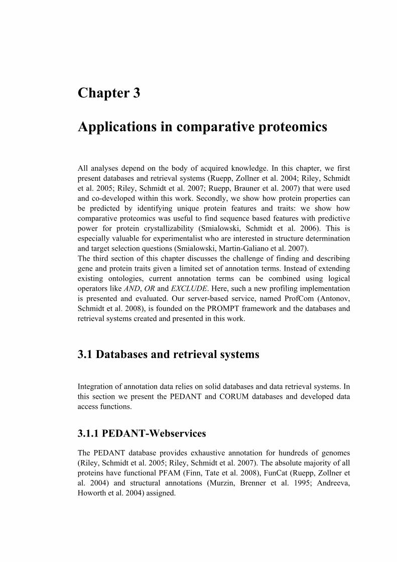
Chapter 3 Applications in comparative proteomics
All analyses depend on the body of acquired knowledge. In this chapter, we first present databases and retrieval systems (Ruepp, Zollner et al. 2004; Riley, Schmidt et al. 2005; Riley, Schmidt et al. 2007; Ruepp, Brauner et al. 2007) that were used and co-developed within this work. Secondly, we show how protein properties can be predicted by identifying unique protein features and traits: we show how comparative proteomics was useful to find sequence based features with predictive power for protein crystallizability (Smialowski, Schmidt et al. 2006). This is especially valuable for experimentalist who are interested in structure determination and target selection questions (Smialowski, Martin-Galiano et al. 2007). The third section of this chapter discusses the challenge of finding and describing gene and protein traits given a limited set of annotation terms. Instead of extending existing ontologies, current annotation terms can be combined using logical operators like AND, OR and EXCLUDE. Here, such a new profiling implementation is presented and evaluated. Our server-based service, named ProfCom (Antonov, Schmidt et al. 2008), is founded on the PROMPT framework and the databases and retrieval systems created and presented in this work.
3.1 Databases and retrieval systems
Integration of annotation data relies on solid databases and data retrieval systems. In this section we present the PEDANT and CORUM databases and developed data access functions.
3.1.1 PEDANT-Webservices
The PEDANT database provides exhaustive annotation for hundreds of genomes (Riley, Schmidt et al. 2005; Riley, Schmidt et al. 2007). The absolute majority of all proteins have functional PFAM (Finn, Tate et al. 2008), FunCat (Ruepp, Zollner et al. 2004) and structural annotations (Murzin, Brenner et al. 1995; Andreeva, Howorth et al. 2004) assigned.
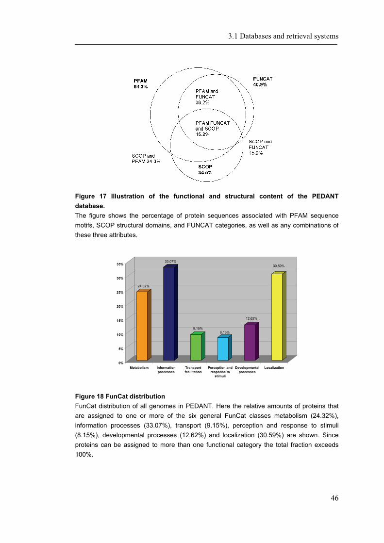
3.1 Databases and retrieval systems
46
Figure 17 Illustration of the functional and structural content of the PEDANT database. The figure shows the percentage of protein sequences associated with PFAM sequence motifs, SCOP structural domains, and FUNCAT categories, as well as any combinations of these three attributes.
Figure 18 FunCat distribution FunCat distribution of all genomes in PEDANT. Here the relative amounts of proteins that are assigned to one or more of the six general FunCat classes metabolism (24.32%), information processes (33.07%), transport (9.15%), perception and response to stimuli (8.15%), developmental processes (12.62%) and localization (30.59%) are shown. Since proteins can be assigned to more than one functional category the total fraction exceeds 100%.
24,32%
33,07%
9,15%8,15%
12,62%
30,59%
0%
5%
10%
15%
20%
25%
30%
35%
Metabolism Informationprocesses
Transportfacilitation
Perception andresponse to
stimuli
Developmentalprocesses
Localization

3.1 Databases and retrieval systems
47
Figure 17 shows a breakdown and contribution of the major information sources. FunCat is a hierarchical multidimensional annotation scheme described in detail in (Ruepp, Zollner et al. 2004). The distribution snap-shot of the major functions attributed to all proteins annotated in the PEDANT database is shown in Figure 18. One of the major practical challenges is to access the wealth of information stored in databases like PEDANT. Due to the mere size and complexity as well as due to the permanent need being up-to-date, such data resources cannot simply being copied and locally installed. Although user-friendly web-interfaces are provided, automated large-scale analyses require programmatic access interfaces to query and retrieve information from the databases. Here, we have developed a set of Web Service methods for the PEDANT databases that allow to query and access all information stored in the PEDANT databases.
Figure 19 Web Service communication schema
Web Services technology is becoming increasingly popular within the bioinformatics community as a means to exploit the large amounts of data, software programs and computing power available at various institutions (Pillai, Silventoinen et al. 2005; Wilkinson, Schoof et al. 2005). According to the World Wide Web Consortium (W3C) a Web Service is a software system designed to support interoperable machine-to-machine interactions over a network (http://www.w3.org/2002/ws/). This technology is based on the eXtensible Markup Language (XML) and open standards, and is platform and programming language independent. This enables clients for a particular service to be written in many
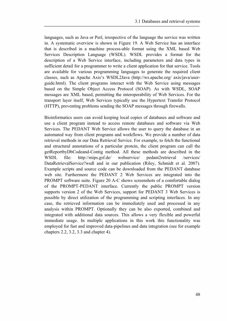
3.1 Databases and retrieval systems
48
languages, such as Java or Perl, irrespective of the language the service was written in. A systematic overview is shown in Figure 19. A Web Service has an interface that is described in a machine process-able format using the XML based Web Services Description Language (WSDL). WSDL provides a format for the description of a Web Service interface, including parameters and data types in sufficient detail for a programmer to write a client application for that service. Tools are available for various programming languages to generate the required client classes, such as Apache Axis’s WSDL2Java (http://ws.apache.org/ axis/java/user-guide.html). The client programs interact with the Web Service using messages based on the Simple Object Access Protocol (SOAP). As with WSDL, SOAP messages are XML based, permitting the interoperability of Web Services. For the transport layer itself, Web Services typically use the Hypertext Transfer Protocol (HTTP), preventing problems sending the SOAP messages through firewalls. Bioinformatics users can avoid keeping local copies of databases and software and use a client program instead to access remote databases and software via Web Services. The PEDANT Web Service allows the user to query the database in an automated way from client programs and workflows. We provide a number of data retrieval methods in our Data Retrieval Service. For example, to fetch the functional and structural annotations of a particular protein, the client program can call the getReportbyDbCodeand-Contig method. All these methods are described in the WSDL file: http://mips.gsf.de/ webservice/ pedant2retrieval /services/ DataRetrievalService?wsdl and in our publication (Riley, Schmidt et al. 2007). Example scripts and source code can be downloaded from the PEDANT database web site. Furthermore the PEDANT 2 Web Services are integrated into the PROMPT software suite. Figure 20 A-C shows screenshots of a comfortable dialog of the PROMPT-PEDANT interface. Currently the public PROMPT version supports version 2 of the Web Services, support for PEDANT 3 Web Services is possible by direct utilization of the programming and scripting interfaces. In any case, the retrieved information can be immediately used and processed in any analysis within PROMPT. Optionally they can be also exported, combined and integrated with additional data sources. This allows a very flexible and powerful immediate usage. In multiple applications in this work this functionality was employed for fast and improved data-pipelines and data integration (see for example chapters 2.2, 3.2, 3.3 and chapter 4).
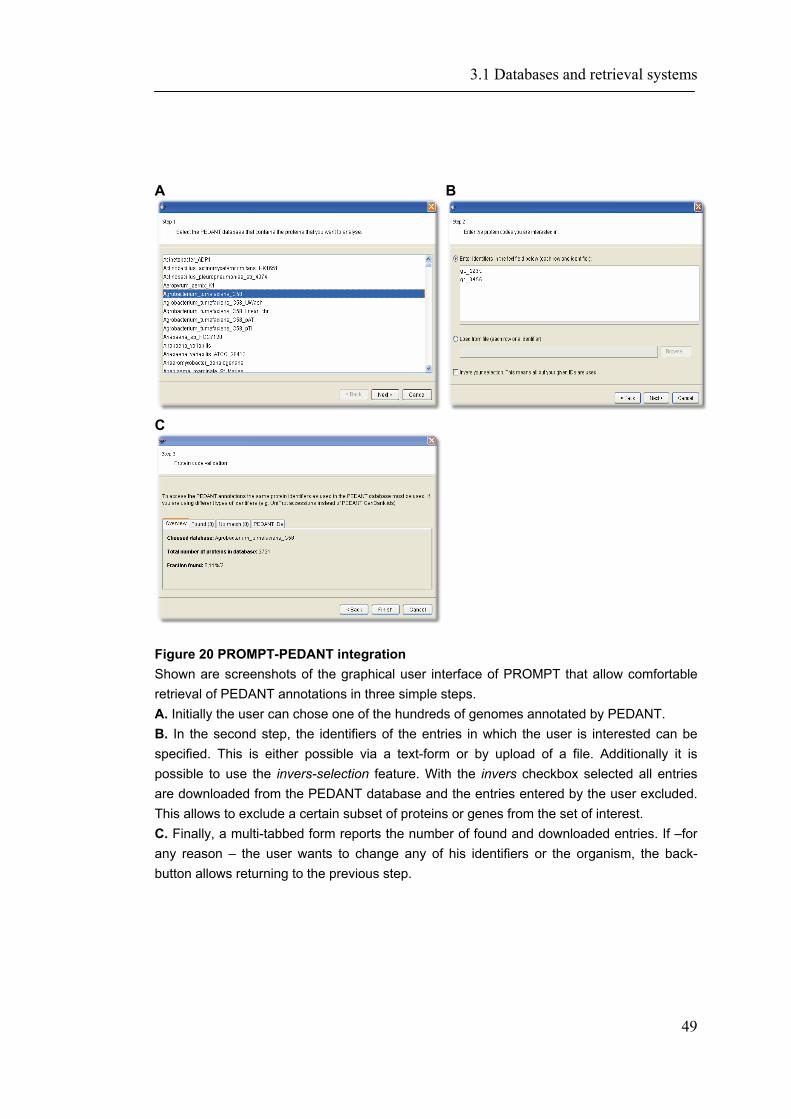
3.1 Databases and retrieval systems
49
A B
C
Figure 20 PROMPT-PEDANT integration Shown are screenshots of the graphical user interface of PROMPT that allow comfortable retrieval of PEDANT annotations in three simple steps. A. Initially the user can chose one of the hundreds of genomes annotated by PEDANT. B. In the second step, the identifiers of the entries in which the user is interested can be specified. This is either possible via a text-form or by upload of a file. Additionally it is possible to use the invers-selection feature. With the invers checkbox selected all entries are downloaded from the PEDANT database and the entries entered by the user excluded. This allows to exclude a certain subset of proteins or genes from the set of interest. C. Finally, a multi-tabbed form reports the number of found and downloaded entries. If –for any reason – the user wants to change any of his identifiers or the organism, the back-button allows returning to the previous step.
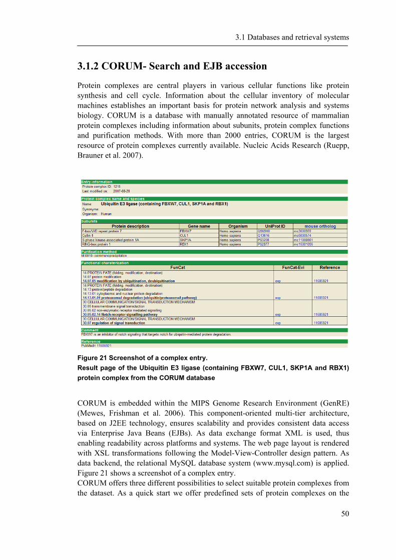
3.1 Databases and retrieval systems
50
3.1.2 CORUM- Search and EJB accession
Protein complexes are central players in various cellular functions like protein synthesis and cell cycle. Information about the cellular inventory of molecular machines establishes an important basis for protein network analysis and systems biology. CORUM is a database with manually annotated resource of mammalian protein complexes including information about subunits, protein complex functions and purification methods. With more than 2000 entries, CORUM is the largest resource of protein complexes currently available. Nucleic Acids Research (Ruepp, Brauner et al. 2007).
Figure 21 Screenshot of a complex entry. Result page of the Ubiquitin E3 ligase (containing FBXW7, CUL1, SKP1A and RBX1) protein complex from the CORUM database
CORUM is embedded within the MIPS Genome Research Environment (GenRE) (Mewes, Frishman et al. 2006). This component-oriented multi-tier architecture, based on J2EE technology, ensures scalability and provides consistent data access via Enterprise Java Beans (EJBs). As data exchange format XML is used, thus enabling readability across platforms and systems. The web page layout is rendered with XSL transformations following the Model-View-Controller design pattern. As data backend, the relational MySQL database system (www.mysql.com) is applied. Figure 21 shows a screenshot of a complex entry. CORUM offers three different possibilities to select suitable protein complexes from the dataset. As a quick start we offer predefined sets of protein complexes on the
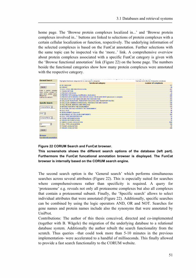
3.1 Databases and retrieval systems
51
home page. The ‘Browse protein complexes localized in...’ and ‘Browse protein complexes involved in..’ buttons are linked to selections of protein complexes with a certain cellular localization or function, respectively. The underlying information of the selected complexes is based on the FunCat annotation. Further selections with the same topic can be inspected via the ‘more..’ link. A comprehensive overview about protein complexes associated with a specific FunCat category is given with the ‘Browse functional annotation’ link (Figure 22) on the home page. The numbers beside the functional categories show how many protein complexes were annotated with the respective category.
Figure 22 CORUM Search and FunCat browser. This screenshots shows the different search options of the database (left part). Furthermore the FunCat funcational annotation browser is displayed. The FunCat browser is internally based on the CORUM search engine.
The second search option is the ‘General search’ which performs simultaneous searches across several attributes (Figure 22). This is especially suited for searches where comprehensiveness rather than specificity is required. A query for ‘proteasome’ e.g. reveals not only all proteasome complexes but also all complexes that contain a proteasomal subunit. Finally, the ‘Specific search’ allows to select individual attributes that were annotated (Figure 22). Additionally, specific searches can be combined by using the logic operators AND, OR and NOT. Searches for gene names and protein names include also the synonyms that were annotated by UniProt. Contributions: The author of this thesis conceived, directed and co-implemented (together with B. Wägele) the migration of the underlying database to a relational database system. Additionally the author rebuilt the search functionality from the scratch. Thus queries –that could took more than 5-10 minutes in the previous implementation- were accelerated to a handful of milliseconds. This finally allowed to provide a fast search functionality to the CORUM website.
3.2 Comparative analyses for structural bioinformatics
In the following section we show the usefulness of comparative approaches to determine features that are relevant for protein structure determination experiments. In this example application, sequence-based features were resolved that allow a prediction of protein crystallizability (Smialowski, Schmidt et al. 2006). This part was done in cooperation with P. Smialowsiki, J. Cox, A. Kirschner and D. Frishman. J. Cox contributed to the machine learning optimization, A. Kirschner provided the secondary structure feature used in this study and P. Smialowski coordinated the project. This section 3.2 demonstrates how the developed methodology (see previous chapters) can yield to new insights. In the subsequent sections we will give a short background about structure determination, limitations and prospects, outline very briefly the basic bioinformatic concepts and conclude with a concise summary of the results.
3.2.1 Background
The ultimate goal of structural genomics is to determine structures for every natural protein through both a large-scale experimental structure characterization and computational analysis. However, in anticipation of the development of cost-effective techniques, current efforts in structural genomics are aimed towards determining structures of limited portion of representative proteins to achieve coverage of the protein structure and function space (Frishman 2002). Nuclear Magnetic Resonance (NMR) spectroscopy and X-ray crystallography are the prevalent methods of structure determination that can contribute to the rapid production of structures. Even though X-ray crystallography is leading technique used for structure elucidation it also has serious deficiencies. A major factor that limits the success of large-scale structure determination efforts is the intrinsic difficulty in obtaining well diffracting crystals for X-ray analysis. The choice of experimental conditions for protein production and crystallization remains a tedious trial-and-error process with uncertain outcome. The preparation of protein samples to yield good quality structural data is considered to be the most time-consuming phase of the structural proteomics program (Yee, Pardee et al. 2003). It was reported (Yee, Pardee et al. 2003) that during pilot Methanobacterium thermoautotrophicum structural genomic project only some 42 % of the purified proteins that went into initial crystallization trials crystallized. Nowadays it is apparent that any structural genomics project would enormously benefit if a rational strategy exist that allows to filter out potentially recalcitrant proteins or, to determine at least in some cases the chances of protein to crystallize. At the current pace of structural genomics even a
3.2 Comparative analyses for structural bioinformatics
53
minimal advance in this direction leading to improvement of success rate by just a few percentage points would translate into significant reduction of cost and yield dozens of additional structures. Although factors determining protein crystallizability are generally poorly understood and elusive, recently there were many attempts to data mine “pipeline” of structural genomics in aim to characterize the differences between proteins which are successfully progressing throughout research stages (cloning, expression, purification, crystallization, structure determination) and those which are recalcitrant (Christendat, Yee et al. 2000; Bertone, Kluger et al. 2001; Goh, Lan et al. 2004). The most comprehensive effort so far was the study of Goh and coworkers (Goh, Lan et al. 2004). Authors made systematic statistical characterization of 27000 proteins from TargetDB (Chen, Oughtred et al. 2004). They calculated average features of proteins from different stages of structural genomics “pipeline” and found that there is a correlation between average proteins characteristics and its progress through each stage of the structural genomics pipeline, from cloning, expression, purification, and ultimately to structural determination. By using tree-based analysis they rate significance of features in protein’s amenability throughout high-throughput experimentation. The most pronounced differences between structurally determined targets and all targets from TargetDB are that the earlier have: higher degree of conservation throughout the organisms; higher percentage composition of charged residues; lower occurrence of hydrophobic patterns; shorter length of hydrophobic stretches; lower number of interacting partners and shorter protein sequence. Unlike research of Goh and coworkers (Goh, Lan et al. 2004) which was primarily analyzing differences among groups of proteins we attempt to developed a general computational technique to classify protein sequences between two groups. We use this method to assess the feasibility of proteins for crystallization solely based on sequence information and independent of protein length.
3.2.2 Material and Methods
Datasets
The primary datasets used for this analysis were collected by P. Smialowski. Briefly, protein sequences with a length range of 30 and 200 amino acids were collected from the PDB database (Berman, Westbrook et al. 2000) and split accordingly to the experimental methods by which the structure was resolved. The resulting datasets XRAY (resolved by X-ray diffraction) and NMR (resolved by Nuclear Magnetic Resonance) were further filtered accordingly to their sequence similarity: NMR sequences without any homology to XRAY sequences (BLAST bit score cut-off less than 30) make up the NMR_ONLY dataset. Proteins with a comparable length (at maximum 10% difference) and high sequence similarity (>75%) build the
3.2 Comparative analyses for structural bioinformatics
54
XRAY_NMR dataset. All datasets were made non-redundant with the tool CD-Hit (Li, Jaroszewski et al. 2001; Li, Jaroszewski et al. 2002) at 50% sequence identity level. Further datasets and details are described in detail in the supplements of our publication (Smialowski, Schmidt et al. 2006).
Adjustment of sequence length distributions
The three raw datasets (NMR_ONLY, XRAY_NMR and XRAY) have significantly different protein length distribution. This is a result of the increasing experimental difficulty to use NMR with larger proteins. To avoid a classifier prediction based on sequence length, the training datasets were adjusted via sampling from the more populated set so that protein length distributions are comparable and not revocable by a Kolmogorov-Smirnov test. This resulted in multiple datasets and combinations thereof. Although P. Smialowski and the author of this thesis evaluated all of them (see our paper and supplements for full details), the following will focus on the smaller but more conceive dataset that was used in the training of the final classifier. An evaluation of all dataset and combinations thereof can be found in the supplements of (Smialowski, Schmidt et al. 2006).
Protein sequence features
Frequencies of mono-, di-, and tri-peptides can be used to represent protein sequences for classification. However, the space of peptide frequencies rapidly becomes very highly-dimensional with growing peptide length. Increasing the peptide size by one, results in multiplying the number of features by a factor of twenty. To reduce the dimensionality of the feature space we decided to cluster the amino acids into groups with similar physico-chemical or structural properties. Given that structural redundancy exists in the amino acid code, it is reasonable to assume that a collapse of the twenty letter alphabet to a suitable condensed version will not lead to a strong loss of information. Utilization of a reduced alphabet also results in larger counts of individual words which increases the signal-to-noise ratio. For the original amino acid alphabet we calculated the frequencies of words of length one and two while for condensed alphabets, words of length one, two, and three were considered. In the following, we describe the alphabets used in this work. All alphabets and groupings are implemented in the PROMPT framework (see chapter 2) and can be used readily in any further application. Counting single amino acid and dipeptides frequencies we obtained attribute spaces of dimensions 20 and 400, respectively. Furthermore the hydrophobicity of amino acids was taken under consideration: Each amino acid sequence was represented in the new alphabet as a sequence of hydrophobicity classes, and the percentages of corresponding words of length one, two, and three were recorded. As a result, each protein was represented by a vector of 3, 9, or 27 numbers for each of the hydrophobicity scales considered. Amino acids were clustered using the
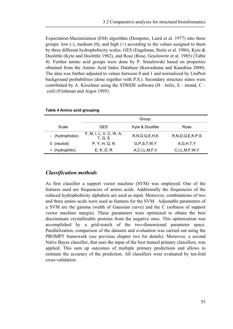
3.2 Comparative analyses for structural bioinformatics
55
Expectation-Maximization (EM) algorithm (Dempster, Laird et al. 1977) into three groups: low (-), medium (0), and high (+) according to the values assigned to them by three different hydrophobicity scales: GES (Engelman, Steitz et al. 1986), Kyte & Doolittle (Kyte and Doolittle 1982), and Rose (Rose, Geselowitz et al. 1985) (Table 4). Further amino acid groups were done by P. Smialowski based on properties obtained from the Amino Acid Index Database (Kawashima and Kanehisa 2000). The data was further adjusted to values between 0 and 1 and normalized by UniProt background probabilities (done together with P.S.). Secondary structure states were contributed by A. Kirschner using the STRIDE software (H – helix, E – strand, C – coil) (Frishman and Argos 1995).
Table 4 Amino acid grouping
Group
Scale GES Kyte & Doolittle Rose
- (hydrophobic) F, M, I, L, V, C, W, A, T, G, S R,N,D,Q,E,H,K R,N,D,Q,E,K,P,S
0 (neutral) P, Y, H, Q, N G,P,S,T,W,Y A,G,H,T,Y
+ (hydrophilic) E, K, D, R A,C,I,L,M,F,V C,I,L,M,F,W,V
Classification methods
As first classifier a support vector machine (SVM) was employed. One of the features used are frequencies of amino acids. Additionally the frequencies of the reduced hydrophobicity alphabets are used as input. Moreover, combinations of two and three amino acids were used as features for the SVM. Adjustable parameters of a SVM are the gamma (width of Gaussian curve) and the C (softness of support vector machine margin). These parameters were optimized to obtain the best discriminate crystallizable proteins from the negative ones. This optimization was accomplished by a grid-search of the two-dimensional parameter space. Parallelization, comparison of the datasets and evaluation was carried out using the PROMPT framework (see previous chapter two for details). Moreover, a second Naïve Bayes classifier, that uses the input of the best trained primary classifiers, was applied. This sum up outcomes of multiple primary predictions and allows to estimate the accuracy of the prediction. All classifiers were evaluated by ten-fold cross-validation.
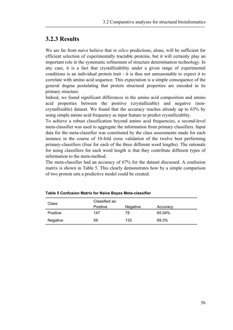
3.2 Comparative analyses for structural bioinformatics
56
3.2.3 Results
We are far from naive believe that in silico predictions, alone, will be sufficient for efficient selection of experimentally tractable proteins, but it will certainly play an important role in the systematic refinement of structure determination technology. In any case, it is a fact that crystallizability under a given range of experimental conditions is an individual protein trait - it is thus not unreasonable to expect it to correlate with amino acid sequence. This expectation is a simple consequence of the general dogma postulating that protein structural properties are encoded in its primary structure. Indeed, we found significant differences in the amino acid composition and amino acid properties between the positive (crystallizable) and negative (non-crystallizable) dataset. We found that the accuracy reaches already up to 63% by using simple amino acid frequency as input feature to predict crystallizablity. To achieve a robust classification beyond amino acid frequencies, a second-level meta-classifier was used to aggregate the information from primary classifiers. Input data for the meta-classifier was constituted by the class assessments made for each instance in the course of 10-fold cross validation of the twelve best performing primary-classifiers (four for each of the three different word lengths). The rationale for using classifiers for each word length is that they contribute different types of information to the meta-method. The meta-classifier had an accuracy of 67% for the dataset discussed. A confusion matrix is shown in Table 5. This clearly demonstrates how by a simple comparison of two protein sets a predictive model could be created.
Table 5 Confusion Matrix for Naive Bayes Meta-classifier
Class Classified as: Positive Negative Accuracy
Positive 147 79 65.04%
Negative 59 133 69.3%
3.3 Complex functional profiling of protein and gene sets
In the previous section we showed how protein crystallizability could be addressed by comparing crystallizable versus non-crystallizable protein sets and described associated protein traits. We thus showed how by comparative approaches and our developed technology difficult problems can be addressed. However, in scientific rationales with increasingly complexity, rare sets of features may not be sufficient for an adequate description of the traits of gene and protein sets. Therefore it is an advantage to combine annotation features using (logical) operators. In the following a system for complex function profiling is described and new significant properties of gene sets related to ovarian and prostate cancer are discussed (Antonov, Schmidt et al. 2008). The presented web-tool is specially suited for a functional analysis of gene and protein sets. Beyond, it allows to analyze any custom datasets and annotation types via additional Web Services. This section starts with a short introduction into the field of functional profiling and outlines how the developed technology is based on- and adds to the PROMPT framework (see chapter 2 for details). Finally new insights into the complex functionality of regulated genes in cancer cells are presented and discussed.
3.3.1 Introduction
Relating experimental data to biological knowledge is a necessity to cope with the data avalanches emerging from recent developments in high-throughput technologies. Automatic functional profiling has become the de facto approach for the secondary analysis of high throughput data. A number of tools employing available gene functional annotations as well as pathway databases have been developed (Khatri, Draghici et al. 2002; Berriz, King et al. 2003; Zeeberg, Feng et al. 2003; Al-Shahrour, az-Uriarte et al. 2004; Khatri, Bhavsar et al. 2004; Martin, Brun et al. 2004; Masseroli, Martucci et al. 2004; Al-Shahrour, Minguez et al. 2005; Zhang, Kirov et al. 2005; Al-Shahrour, Minguez et al. 2006; Antonov and Mewes 2006; Antonov, Tetko et al. 2006; Al-Shahrour, Minguez et al. 2007; Carmona-Saez, Chagoyen et al. 2007; Draghici, Khatri et al. 2007; Goffard and Weiller 2007; Khatri, Voichita et al. 2007; Reimand, Kull et al. 2007). The advantages and limitations of most of these tools are reviewed in (Khatri and Draghici 2005). An important aspect of standard functional profiling methodology is inability to overcome the limits of employed annotation vocabularies. Do current annotation vocabularies cover all possible biological functions? Can they cover them in the future? The space of possible biological functions is almost infinite. However to control it one does not need an infinite number of functional terms. Consider a very
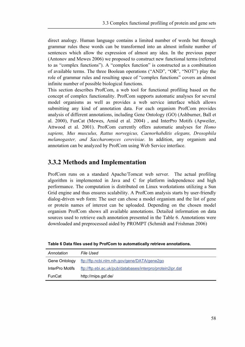
3.3 Complex functional profiling of protein and gene sets
58
direct analogy. Human language contains a limited number of words but through grammar rules these words can be transformed into an almost infinite number of sentences which allow the expression of almost any idea. In the previous paper (Antonov and Mewes 2006) we proposed to construct new functional terms (referred to as “complex functions”). A “complex function” is constructed as a combination of available terms. The three Boolean operations (“AND”, “OR”, “NOT”) play the role of grammar rules and resulting space of “complex functions” covers an almost infinite number of possible biological functions. This section describes ProfCom, a web tool for functional profiling based on the concept of complex functionality. ProfCom supports automatic analyses for several model organisms as well as provides a web service interface which allows submitting any kind of annotation data. For each organism ProfCom provides analysis of different annotations, including Gene Ontology (GO) (Ashburner, Ball et al. 2000), FunCat (Mewes, Amid et al. 2004) , and InterPro Motifs (Apweiler, Attwood et al. 2001). ProfCom currently offers automatic analyses for Homo sapiens, Mus musculus, Rattus norvegicus, Caenorhabditis elegans, Drosophila melanogaster, and Saccharomyces cerevisiae. In addition, any organism and annotation can be analyzed by ProfCom using Web Service interface.
3.3.2 Methods and Implementation
ProfCom runs on a standard Apache/Tomcat web server. The actual profiling algorithm is implemented in Java and C for platform independence and high performance. The computation is distributed on Linux workstations utilizing a Sun Grid engine and thus ensures scalability. A ProfCom analysis starts by user-friendly dialog-driven web form: The user can chose a model organism and the list of gene or protein names of interest can be uploaded. Depending on the chosen model organism ProfCom shows all available annotations. Detailed information on data sources used to retrieve each annotation presented in the Table 6. Annotations were downloaded and preprocessed aided by PROMPT (Schmidt and Frishman 2006)
Table 6 Data files used by ProfCom to automatically retrieve annotations.
Annotation File Used
Gene Ontology ftp://ftp.ncbi.nlm.nih.gov/gene/DATA/gene2go
InterPro Motifs ftp://ftp.ebi.ac.uk/pub/databases/interpro/protein2ipr.dat
FunCat http://mips.gsf.de/

3.3 Complex functional profiling of protein and gene sets
59
ProfCom is resolving synonyms and annotation data automatically and returns the percentage of recognized identifiers immediately using the PROMPT framework as backend. At the first step user supplied gene IDs are mapped to “Entrez Gene” identifiers. For this purpose synonymous list from NCBI and Affymetrix web sites are used. Detailed information on data sources used by ProfCom are shown in Table 7.
Table 7 Types of gene identifiers recognized by ProfCom and data sources used for ID mapping.
Type Of Ids File Used
“Gene Symbol”, “Ensembl”, “LocusTag”
ftp://ftp.ncbi.nlm.nih.gov/gene/DATA/gene_info.gz
“RefSeq Protein ID”, “RefSeq Transcript ID” ftp://ftp.ncbi.nlm.nih.gov/gene/DATA/gene2refseq.gz
“UniProt/Swiss-Prot” ftp://ftp.ncbi.nlm.nih.gov/gene/DATA/gene_refseq_uniprotkb_collab.gz
“UniGene” ftp://ftp.ncbi.nlm.nih.gov/gene/DATA/gene2unigene
“Affymetrix probe codes” http://www.affymetrix.com/ Annotation files
The profiling algorithm is implemented as described in (Antonov and Mewes 2006). Briefly, a greedy-search through the space of annotation tupels is performed. The complex annotation functions’ statistical significance is evaluated by a Monte-Carlo simulation after each level-wise iteration.
3.3.3 Results
Automatically Supported Annotations and Gene Ids
As input ProfCom accepts several types of gene or protein identifiers. For example, for human genome ProfCom supports identifiers of “Entrez Gene”(Wheeler, Barrett et al. 2006), “UniProt/Swiss-Prot” , “Gene Symbol” (Wheeler, Barrett et al. 2006; Wheeler, Barrett et al. 2007), “UniGene”(Wheeler, Barrett et al. 2006), Ensembl”(Birney, Andrews et al. 2006) , “RefSeq Protein ID”, “RefSeq Transcript ID”(Pruitt, Tatusova et al. 2007), and “Affymetrix probe codes” (Liu, Loraine et al. 2003). Additionally a mixture of several identifier types is possible. The user gets full information on mapping of the supplied gene IDs. It includes 4 result tables. The first ProfCom result table reports full mapping details of
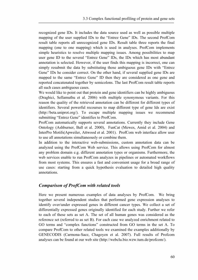
3.3 Complex functional profiling of protein and gene sets
60
recognized gene IDs. It includes the data source used as well as possible multiple mapping of the user supplied IDs to the “Entrez Gene” IDs. The second ProfCom result table reports all unrecognized gene IDs. Result table three reports the final mapping (one to one mapping) which is used in analyses. ProfCom implements simple heuristics to resolve multiple mapping issues. Among possibilities to map user gene ID to the several “Entrez Gene” IDs, the IDs which has most abundant annotation is selected. However, if the user finds this mapping is incorrect, one can simply resubmit the data by substituting those ambiguous gene IDs with “Entrez Gene” IDs he consider correct. On the other hand, if several supplied gene IDs are mapped to the same “Entrez Gene” ID then they are considered as one gene and reported concatenated together by semicolons. The last ProfCom result table reports all such cases ambiguous cases. We would like to point out that protein and gene identifiers can be highly ambiguous (Draghici, Sellamuthu et al. 2006) with multiple synonymous variants. For this reason the quality of the retrieved annotation can be different for different types of identifiers. Several powerful recourses to map different type of gene Ids are exist (http://beta.uniprot.org/). To escape multiple mapping issues we recommend submitting “Entrez Gene” identifies to ProfCom. ProfCom automatically supports several annotations. Currently they include Gene Ontology (Ashburner, Ball et al. 2000), FunCat (Mewes, Amid et al. 2004) and InterPro Motifs(Apweiler, Attwood et al. 2001). ProfCom web interface allow user to use all annotations simultaneously or combine them. In addition to the interactive web-submissions, custom annotation data can be analyzed using the ProfCom Web service. This allows using ProfCom for almost any problem domain e.g. different annotation types or organisms. Furthermore, the web services enable to run ProfCom analyzes in pipelines or automated workflows from most systems. This ensures a fast and convenient usage for a broad range of use cases: starting from a quick hypothesis evaluation to detailed high quality annotations.
Comparison of ProfCom with related tools
Here we present numerous examples of data analyses by ProfCom. We bring together several independent studies that performed gene expression analyses to identify over/under expressed genes in different cancer types. We collect a set of differentially expressed genes originally identified for each study. Further we refer to each of these sets as set A. The set of all human genes was considered as the reference set (referred to as set B). For each case we analyzed enrichment related to GO terms and “complex functions” constructed from GO terms in the set A. To compare ProfCom to other related tools we examined the examples additionally by GENECODIS (Carmona-Saez, Chagoyen et al. 2007). Full results of Profcom analyses can be found at our web site (http://webclu.bio.wzw.tum.de/profcom/).
3.3 Complex functional profiling of protein and gene sets
61
Example 1. Gene Expression in Ovarian Cancer Reflects Both Morphology and Biological Behavior, Distinguishing Clear Cell from Other Poor-Prognosis Ovarian Carcinomas
Gene expression in 113 ovarian epithelial tumors using oligonucleotide microarrays was analyzed (Schwartz, Kardia et al. 2002). In total, 73 genes, expressed 2- to 29-fold higher in clear cell ovarian carcinoma compared with each of the other ovarian carcinoma types, were identified. Standard functional profiling of these genes reveals statistically significant enrichments related to several GO terms. One of the enriched terms was “cell adhesion”. In the set A of 73 up-regulated genes 10 genes belonged to this category while 390 genes classified by this term in all human genome. This group of genes may be of particular interest as it was shown in different studies that cell adhesion molecules can play important role in epithelial ovarian cancer development (Hong, Baudhuin et al. 1999; Spizzo, Went et al. 2006). By analyses of relation between GO terms in the set A, ProfCom classify these genes more specifically. The complex function “cell adhesion EXCLUDING homophilic cell adhesion EXCLUDING structural molecule activity” inferred by ProfCom classifies only 245 (compare to 390) genes in the whole genome and all 10 genes in the set A. The resolved complex function is more specific (the same selectivity with almost 2-fold increase in specificity). In addition, this information may be useful to analyze cancer molecular mechanisms. GENECODIS detects single GO term “cell adhesion” as being overrepresented. However, no other evidences that can be helpful to understand the role of up-regulated “cell adhesion” genes were provided.
Example 2. Comprehensive Gene Expression Analysis of Prostate Cancer Reveals Distinct Transcriptional Programs Associated with Metastatic Disease
The study of LaTulippe and co-workers (LaTulippe, Satagopan et al. 2002) performs a comprehensive gene expression analysis of prostate cancer using oligonucleotide arrays with 63,175 probe sets to identify genes with strong differential expression between non-recurrent primary prostate cancers and metastatic prostate cancers. Among highly ranked over-expressed genes (73 genes selected based on the t test statistic) by manual analyses the authors found genes that participate in cell cycle regulation, DNA replication, and DNA repair. Standard functional profiling of these genes reveals statistically significant enrichments related to several GO terms. For example, a subset of 10 from 73 over-expressed genes was related by term “regulation of progression through cell cycle”. This category may be relevant for understanding of transcriptional programs associated with metastatic disease. According to GO annotation, the term “regulation of progression through cell cycle” unites approximately 160 genes in human genome. It is clear that only a fraction of genes classified by this term may be involved in the molecular model of cancer.
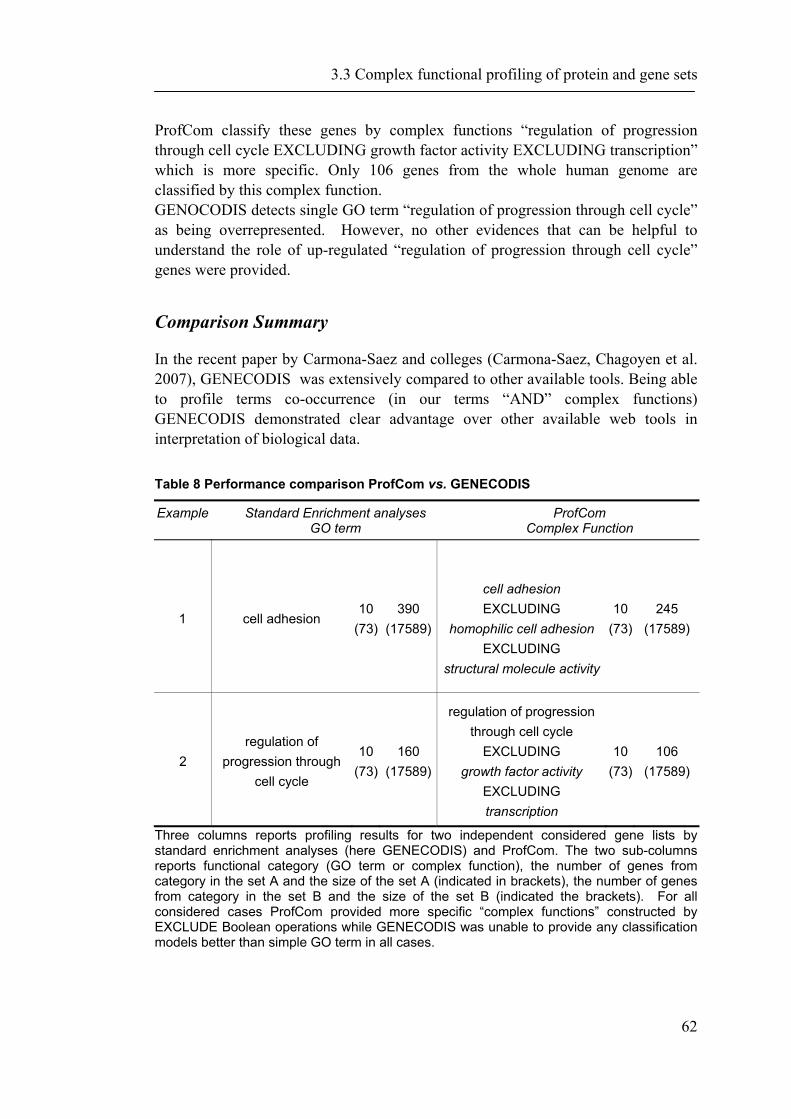
3.3 Complex functional profiling of protein and gene sets
62
ProfCom classify these genes by complex functions “regulation of progression through cell cycle EXCLUDING growth factor activity EXCLUDING transcription” which is more specific. Only 106 genes from the whole human genome are classified by this complex function. GENOCODIS detects single GO term “regulation of progression through cell cycle” as being overrepresented. However, no other evidences that can be helpful to understand the role of up-regulated “regulation of progression through cell cycle” genes were provided.
Comparison Summary
In the recent paper by Carmona-Saez and colleges (Carmona-Saez, Chagoyen et al. 2007), GENECODIS was extensively compared to other available tools. Being able to profile terms co-occurrence (in our terms “AND” complex functions) GENECODIS demonstrated clear advantage over other available web tools in interpretation of biological data.
Table 8 Performance comparison ProfCom vs. GENECODIS
Example
Standard Enrichment analyses GO term
ProfCom Complex Function
1 cell adhesion 10
(73)390
(17589)
cell adhesion EXCLUDING
homophilic cell adhesion EXCLUDING
structural molecule activity
10 (73)
245 (17589)
2 regulation of
progression through cell cycle
10(73)
160 (17589)
regulation of progression through cell cycle
EXCLUDING growth factor activity
EXCLUDING transcription
10 (73)
106 (17589)
Three columns reports profiling results for two independent considered gene lists by standard enrichment analyses (here GENECODIS) and ProfCom. The two sub-columns reports functional category (GO term or complex function), the number of genes from category in the set A and the size of the set A (indicated in brackets), the number of genes from category in the set B and the size of the set B (indicated the brackets). For all considered cases ProfCom provided more specific “complex functions” constructed by EXCLUDE Boolean operations while GENECODIS was unable to provide any classification models better than simple GO term in all cases.
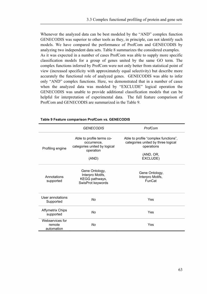
3.3 Complex functional profiling of protein and gene sets
63
Whenever the analyzed data can be best modeled by the “AND” complex function GENECODIS was superior to other tools as they, in principle, can not identify such models. We have compared the performance of ProfCom and GENECODIS by analyzing two independent data sets. Table 8 summarizes the considered examples. As it was expected in a number of cases ProfCom was able to supply more specific classification models for a group of genes united by the same GO term. The complex functions inferred by ProfCom were not only better from statistical point of view (increased specificity with approximately equal selectivity) but describe more accurately the functional role of analyzed genes. GENECODIS was able to infer only “AND” complex functions. Here, we demonstrated that in a number of cases when the analyzed data was modeled by “EXCLUDE” logical operation the GENECODIS was unable to provide additional classification models that can be helpful for interpretation of experimental data. The full feature comparison of ProfCom and GENECODIS are summarized in the Table 9.
Table 9 Feature comparison ProfCom vs. GENECODIS
GENECODIS ProfCom
Profiling engine
Able to profile terms co-occurrence,
categories united by logical operation
(AND)
Able to profile “complex functions”, categories united by three logical
operations
(AND, OR, EXCLUDE)
Annotations supported
Gene Ontology, Interpro Motifs,
KEGG pathways, SwisProt keywords
Gene Ontology, Interpro Motifs,
FunCat
User annotations Supported No Yes
Affymetrix Chips supported No Yes
Webservices for remote
automation No Yes
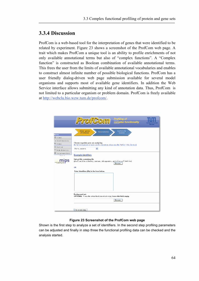
3.3 Complex functional profiling of protein and gene sets
64
3.3.4 Discussion
ProfCom is a web-based tool for the interpretation of genes that were identified to be related by experiment. Figure 23 shows a screenshot of the ProfCom web page. A trait which makes ProfCom a unique tool is an ability to profile enrichments of not only available annotational terms but also of “complex functions”. A “Complex function” is constructed as Boolean combination of available annotational terms. This frees the user from the limits of available annotational vocabularies and enables to construct almost infinite number of possible biological functions. ProfCom has a user friendly dialog-driven web page submission available for several model organisms and supports most of available gene identifiers. In addition the Web Service interface allows submitting any kind of annotation data. Thus, ProfCom is not limited to a particular organism or problem domain. ProfCom is freely available at http://webclu.bio.wzw.tum.de/profcom/.
Figure 23 Screenshot of the ProfCom web page Shown is the first step to analyze a set of identifiers. In the second step profiling parameters can be adjusted and finally in step three the functional profiling data can be checked and the analysis started.
Chapter 4 Gene and protein expression
In this chapter we apply the developed methods and technologies presented the previous chapters at large-scale to biological problem sets. In the first section 4.1 we present the to-date largest protein abundance proteine profiling of the E.coli bacteria. In the second section 4.2 we analyse the structure of underlying genomic archictures that are associated with gene and protein expression.
4.1 Abundance profiling of the E.coli proteome
Knowledge about the abundance of molecular components is an important prerequisite for building quantitative predictive models of cellular behavior. Proteins are central components of these models, since they carry out most of the fundamental processes in the cell. In this section we describe the application of our developed technology at large-scale to protein abundance data of the E.coli proteome (Ishihama, Schmidt et al. 2008).
4.1.1 Introduction
Proteins fulfill a wide variety of functions and are central to almost all processes in living cells. In order to improve our understanding of the complex network of protein interactions in the cell, it is of central importance to obtain information about the activities of the individual components; these are directly linked to their cellular concentrations. The fast development of genomic and proteomic methods has already revealed the basic protein inventory of a few hundred different organisms, but large scale quantitative information on protein concentrations is still largely missing. Comprehensive analyses of cellular mRNA levels have proven to be highly useful tools to monitor the state of a cell, but by design they are missing all influences of the vast amount of posttranscriptional regulations. One of the few organisms where direct protein concentrations are available on a nearly proteome wide level is the yeast Saccharomyces cerevisiae. It has been subject to large scale protein quantification using epitope tagging of virtually the whole proteome followed by quantitative western blotting (Ghaemmaghami, Huh et
4.1 Abundance profiling of the E.coli proteome
66
al. 2003) and to single cell based quantitative proteomic analysis using flow-cell cytometry and a library of GFP-tagged yeast strains (Newman, Ghaemmaghami et al. 2006). While both methods provided high-quality abundance data for nearly the entire proteome, their dependence on the availability of a strain library containing tagged versions of all proteins of interest presents a serious limitation. Depending on the organism under study, to generate such a library may involve an immense amount of work or may even be impossible to achieve. The proteomics field and its key technology mass spectrometry are developing rapidly from qualitative towards quantitative measurements without the need for individual tagging of proteins. These efforts, however, are mostly restricted to the comparison of relative concentrations of the same proteins in different samples. Direct, non-relative abundance data of proteins, allowing a comparison of different proteins within and between samples, are still difficult to obtain on a large scale as reviewed in the first chapter. Here we present a protein abundance analysis of the E.coli proteome with regard to genomic, proteomic, functional and structural features. E. coli is a Gram-negative bacterium of the family Enterobacteriacae. Due to its simple cellular structure and the relative ease of its cultivation and biological modification, it has become the standard ‘workhorse’ of molecular biology, genetics and biotechnology. This resulted in E. coli becoming one of the most completely characterized organisms in biology. The genome of the laboratory strain E. coli K12 has been among the first organisms to be completely sequenced (Blattner, Plunkett et al. 1997). It has a relatively small size of ~ 4.6 Mb, and is predicted to code for approximately 4300 proteins. The genes, proteins, biochemical pathways and molecular interactions in E. coli have been subject to countless experimental studies and the growing number of available information in large scale databases like Genbank and Swiss-Prot, but also in more specialized database projects like e.g. EcoCyc (Keseler, Collado-Vides et al. 2005) or EchoBase (Misra, Horler et al. 2005) allows easy access to a wealth of information. However, in spite of the combined efforts of the scientific community, the complex network of molecular interactions within living organisms, including E. coli, is still far from being fully understood. Deciphering these interaction networks will be a major task of biology in coming years, and the in the following presented detailed knowledge about the concentrations of the individual parts in the system will be an important step on the way to accomplishing this goal.
4.1.2 Material and Methods
Genome data
Amino acid sequences of all proteins identified in this study were obtained from Swiss-Prot (Boeckmann, Bairoch et al. 2003). Throughout this work the primary Swiss-Prot accession code in conjunction with the Swiss-Prot entry name are used as
4.1 Abundance profiling of the E.coli proteome
67
unique protein identifiers. Codon Adaptation Index values (CAI) according to the method of (Sharp and Li 1987) were used as reported by (Blattner, Plunkett et al. 1997). Classification of E. coli genes into three groups - (E) genes essential for cell growth (essential), (N) those dispensable for cell growth (non-essential), and (U) those unknown to be essential or non-essential - was based on the comprehensive experimental analysis of (Gerdes, Scholle et al. 2003). In the latter work, 630 genes were identified as being essential and 3126 as being dispensable using a genetic fingerprinting technique. Data on predicted expression measure of E. coli proteins (Karlin, Mrazek et al. 2001) were downloaded from the genomic.stanford.edu web server. Proteins possessing significant sequence similarity (BLAST (Altschul, Madden et al. 1997) E-value threshold 0.001) to one or several domains of known three-dimensional structure as classified in the SCOP database (Andreeva, Howorth et al. 2004) were attributed to the corresponding SCOP fold. Assignment of genes to functional roles as defined by the MIPS functional catalog version 1.3 (Ruepp, Zollner et al. 2004) was conducted manually at Biomax Informatics AG. Where necessary, correspondence between published protein datasets and the SwissProt database was established based on sequence identity (at least 98%), with some ambiguous cases resolved manually. Minor discrepancies such as a missing methionine at the sequence start or a single amino acid replacement were tolerated.
Abundance data
Protein abundance measurements were obtained from Yasushi Ishihama. Details about the experimental set-up can be found in our publication (Ishihama, Schmidt et al. 2008). Briefly, we employed approximately 200 LC-MS/MS runs in combination with a variety of peptide/protein fractionation methods, different protease digestion schemes, LC-MS conditions and MS/MS fragmentation. This combined and more stringent dataset yielded a total of 1103 proteins, quantified by emPAI, based on 13469 observed peptides with unique parent ions (10339 unique sequences) from 209 LC-MS/MS runs with less than 5% false positive rate. All all identified proteins and peptides can be found in the supplementary material of our publication (Ishihama, Schmidt et al. 2008) in the Tables S2 and S3). The abundance measurements thus provide ~ 32 – 41 % coverage of the approximately 2680 cytosolic proteins in E. coli, depending on the exact definition of the cytosolic dataset.
Coverage of the cytosolic protein content
To compare the coverage of our experimental cytosol sample with the theoretical protein content of cytosol we combined several recent sources of data as well as bioinformatics prediction techniques. For 13% (568 out of 4289) of E. coli proteins experimentally determined cellular localization information has been reported by Lopez-Campistrous et al. (Lopez-Campistrous, Semchuk et al. 2005). We further
4.1 Abundance profiling of the E.coli proteome
68
utilized the PSORT database (Rey, Acab et al. 2005) version 2.0 that provides localization annotation for 62% of the complete E. coli proteome (2678 proteins). The remaining E. coli proteins are classified in the PSORT database as “unknown” or “unknown with multiple possible localizations”. We complemented this information with the number of transmembrane segments predicted using TMHMM (Krogh, Larsson et al. 2001) version 2.0. Proteins with a high number of predicted transmembrane segments can be safely assumed to be not located within the cytosol. However the TMHMM predictions may lead to an over prediction of cytosolic proteins as this method reliably allows to exclude only those proteins that have multiple integral membrane segments. Furthermore, the possibility of falsely predicted membrane segments needs to be considered. We therefore combined the three data sources described above – the number of transmembrane segments, PSORT localization, and experimental localization - to find the most accurate definition of the E. coli cytosol proteome. First we consider all proteins that have at most one membrane predicted region and are annotated as “cytosolic” or “unknown” in the PSORT database. This criterion would predict 61.46% (2636 of 3289) of the E. coli proteome to be cytosolic (Table 10). The advantage of this estimate is twofold. On the one hand a false positive prediction of one membrane region is still tolerated and thus does not lead to loss of information. On the other hand the intersection with the independent PSORT data ensures that an over prediction of cytosolic proteins is avoided as much as possible. Finally we extend our previous definition and add all proteins that were experimentally determined as cytsolic proteins. This results in 2680 proteins that we adopt as our final estimate of the E. coli cytosol proteome. It is notable that the experimental localization data hardly increase the number of the defined cytosolic proteins (plus 1% or 44 of 2680 difference only). This shows the almost complete overlap of the first definition with the experimentally confirmed protein set and confirms the validly of our approach.
Low vs. high abundance proteins
For convenience we considered proteins with copy number values greater than 2050 (emPAI >29.0) highly abundant, while the rest of the proteins were attributed to the low abundance category. This optimal threshold was automatically found by clustering of the log-copy number values using the Expectation Maximization algorithm (Hartigan 1975) as implemented in the WEKA machine learning workbench (Witten and Frank 2005), version 3.5.6 using default parameters with the number of clusters set to two. As the copy number values are distributed according to the extreme value distribution, they were logarithmized to be useable with the Gaussian distribution approximation in the clustering process.
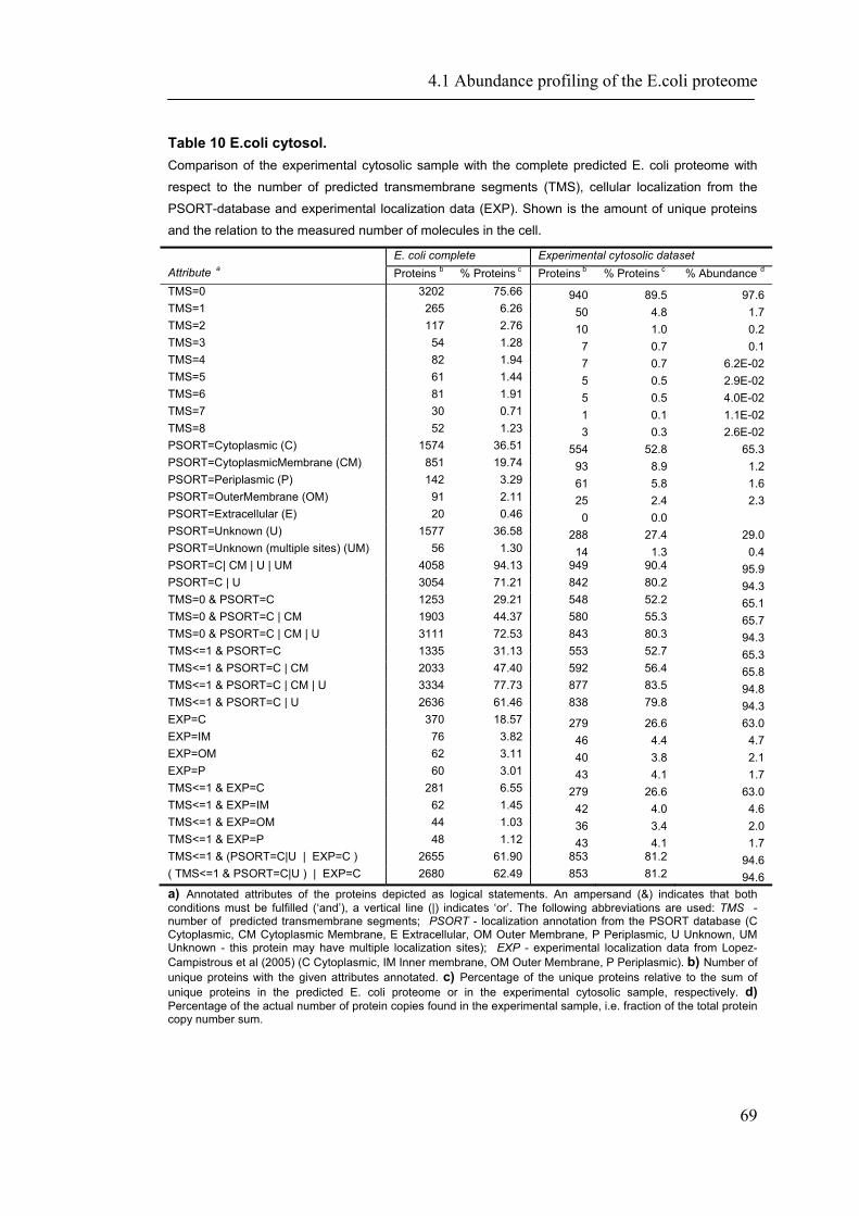
4.1 Abundance profiling of the E.coli proteome
69
Table 10 E.coli cytosol. Comparison of the experimental cytosolic sample with the complete predicted E. coli proteome with
respect to the number of predicted transmembrane segments (TMS), cellular localization from the
PSORT-database and experimental localization data (EXP). Shown is the amount of unique proteins
and the relation to the measured number of molecules in the cell.
Attribute a E. coli complete Experimental cytosolic dataset Proteins b % Proteins c Proteins b % Proteins c % Abundance d
TMS=0 3202 75.66 940 89.5 97.6 TMS=1 265 6.26 50 4.8 1.7 TMS=2 117 2.76 10 1.0 0.2 TMS=3 54 1.28 7 0.7 0.1 TMS=4 82 1.94 7 0.7 6.2E-02 TMS=5 61 1.44 5 0.5 2.9E-02 TMS=6 81 1.91 5 0.5 4.0E-02 TMS=7 30 0.71 1 0.1 1.1E-02 TMS=8 52 1.23 3 0.3 2.6E-02 PSORT=Cytoplasmic (C) 1574 36.51 554 52.8 65.3 PSORT=CytoplasmicMembrane (CM) 851 19.74 93 8.9 1.2 PSORT=Periplasmic (P) 142 3.29 61 5.8 1.6 PSORT=OuterMembrane (OM) 91 2.11 25 2.4 2.3 PSORT=Extracellular (E) 20 0.46 0 0.0 PSORT=Unknown (U) 1577 36.58 288 27.4 29.0 PSORT=Unknown (multiple sites) (UM) 56 1.30 14 1.3 0.4 PSORT=C| CM | U | UM 4058 94.13 949 90.4 95.9 PSORT=C | U 3054 71.21 842 80.2 94.3 TMS=0 & PSORT=C 1253 29.21 548 52.2 65.1 TMS=0 & PSORT=C | CM 1903 44.37 580 55.3 65.7 TMS=0 & PSORT=C | CM | U 3111 72.53 843 80.3 94.3 TMS<=1 & PSORT=C 1335 31.13 553 52.7 65.3 TMS<=1 & PSORT=C | CM 2033 47.40 592 56.4 65.8 TMS<=1 & PSORT=C | CM | U 3334 77.73 877 83.5 94.8 TMS<=1 & PSORT=C | U 2636 61.46 838 79.8 94.3 EXP=C 370 18.57 279 26.6 63.0 EXP=IM 76 3.82 46 4.4 4.7 EXP=OM 62 3.11 40 3.8 2.1 EXP=P 60 3.01 43 4.1 1.7 TMS<=1 & EXP=C 281 6.55 279 26.6 63.0 TMS<=1 & EXP=IM 62 1.45 42 4.0 4.6 TMS<=1 & EXP=OM 44 1.03 36 3.4 2.0 TMS<=1 & EXP=P 48 1.12 43 4.1 1.7 TMS<=1 & (PSORT=C|U | EXP=C ) 2655 61.90 853 81.2 94.6 ( TMS<=1 & PSORT=C|U ) | EXP=C 2680 62.49 853 81.2 94.6 a) Annotated attributes of the proteins depicted as logical statements. An ampersand (&) indicates that both conditions must be fulfilled (‘and’), a vertical line (|) indicates ‘or’. The following abbreviations are used: TMS - number of predicted transmembrane segments; PSORT - localization annotation from the PSORT database (C Cytoplasmic, CM Cytoplasmic Membrane, E Extracellular, OM Outer Membrane, P Periplasmic, U Unknown, UM Unknown - this protein may have multiple localization sites); EXP - experimental localization data from Lopez-Campistrous et al (2005) (C Cytoplasmic, IM Inner membrane, OM Outer Membrane, P Periplasmic). b) Number of unique proteins with the given attributes annotated. c) Percentage of the unique proteins relative to the sum of unique proteins in the predicted E. coli proteome or in the experimental cytosolic sample, respectively. d) Percentage of the actual number of protein copies found in the experimental sample, i.e. fraction of the total protein copy number sum.
4.1 Abundance profiling of the E.coli proteome
70
Statistical methods
All statistical tests and most figures were prepared with the R software package version 2.0 (www.r-project.org) and PROMPT (Schmidt and Frishman 2006). To compare the distributions of two unpaired samples with non-Gaussian or unknown distributions, the rank-sum Mann-Whitney (MW) test and the two sample Kolmogorov-Smirnov (KS) test were applied using the significance threshold α=0.05. The null hypothesis of the Mann-Whitney test is that the abundance means are equal. The null hypothesis of the Kolmogorov-Smirnov test is that the values of the two samples are drawn from the same continuous distributions. Both tests have the advantage that they make no assumptions about the distribution of data. To ensure that our tests are not biased by small sample sizes while comparing essential genes with their counterparts, the test results were verified with additional random sampling whereby each of the applied tests was repeated 105 times with a randomly drawn sample of the associated basic population. Then the p-value of the actual test was compared with the p-value distribution of random samples (data not shown). An observed p-value which lies in the 5% quartile shows a reliable test outcome independently of the sampling bias. Descriptive boxplot distribution statistics such as median, quartiles and outliers were generated with R. According to the canonical statistical definition, values greater than the 3rd quartile plus the inter quartile range (IQR) were considered outliers. The IQR is defined as the 3rd quartile value minus the first quartile value. Relationships between variables were analyzed utilizing the least squares regression, loess estimation and the Pearson or Spearman rank correlation methods implemented in R with default parameters.
Operon structure
A set of known E. coli operons was obtained from RegulonDB (Huerta, Salgado et al. 1998). For all operons with abundance information available for at least 3 proteins the variance of the natural logarithm of the emPAI values was calculated. The variance indicates how similar the abundance of the proteins within each operon is.
Function and structure of proteins
Functional roles of gene products were described in terms of the manually curated hierarchical functional catalog (FUNCAT) (Ruepp, Zollner et al. 2004). In this catalog each of the 16 main classes (e.g., metabolism, energy) may contain up to six subclasses. An essential feature of FUNCAT is its multidimensionality, meaning that any protein can be assigned to multiple categories. Carefully verified manual assignment of E. coli gene products to functional categories was obtained from Biomax Informatics AG (www.biomax.com). Likewise, the SCOP database (Andreeva, Howorth et al. 2004) provides a hierarchical classification of protein
4.1 Abundance profiling of the E.coli proteome
71
structural domains. SCOP fold assignments to gene E. coli products were based on BLAST E-value of 0.001. In this work both FUNCAT and SCOP designators were truncated to include only the two upper levels of hierarchy. Proteins assigned to the same SCOP fold were grouped and the average emPAI value for each group was calculated. To avoid individual outliers with very high or very low expression levels, only groups with 10 or more proteins were considered. The EC Enzyme Nomenclature information was taken from the Swiss-Prot protein descriptions. Disorder predictions were taken from our PEDANT database where they are calculated with the software GlobPlot (Linding, Russell et al. 2003). GlobProt utilizes the statistics of proteins known to have unstructured regions (Wright and Dyson 1999; Tompa 2002). The number of alternating hydrophobic/hydrophilic stretches was computed as described (Wong, Fritz et al. 2005). The residues A, C, F, G, I, L, M, P, V, W and Y were considered to be hydrophobic and H, Q, N, S, T, K, R, D, E were considered hydrophilic in this study. The hydrophobicity of a protein
was defined as n
Hn
i i∑=1 , with iH denoting the hydrophobicity value of the amino
acid at position i of a protein of n amino acids. Hydrophobicity values were calculated using the Kyte-Doolittle scale (Kyte and Doolittle 1982).
4.1 Abundance profiling of the E.coli proteome
72
4.1.3 Results
Large scale determination of protein abundance in the Escherichia coli cytosol.
Approximately 200 individual LC-MS/MS runs were performed of the E. coli MC4100 cytosol, in combination with a variety of protein and peptide separation methods in order to maximize protein identification coverage. A summary and detailed evaluations of the methods employed is given in (Ishihama, Schmidt et al. 2008). The decision to only investigate the cytosol of E. coli, rather than a whole cell lysate, was a direct consequence of our intention to provide reliable concentration estimates of all identified proteins, and avoid technical difficulties frequently arising from the quantitative proteolytic digestion of membrane proteins (Corbin, Paliy et al. 2003; Wu and Yates 2003). In total, 1103 proteins were quantified by emPAI. This result is based on 13469 observed peptides with unique parent ions (10339 unique sequences) from 209 LC-MS/MS runs with less than 5% false positive rate, all data can be found as supplementary material of (Ishihama, Schmidt et al. 2008). Our measurements thus provide ~ 32 – 41 % coverage of the approximately 2680 cytosolic proteins in E. coli, depending on the exact definition of the cytosolic dataset, as defined in Materials and Methods.
Validation of the emPAI-based protein abundance dataset.
To test for potential biases in the peptide identification process we compared a number of physico-chemical properties of the observed peptides with all predicted peptides from the corresponding proteins. These parameters are expected to influence the peptide behavior during many of the employed fractionation and separations steps as for instance chromatography. As listed in Table 11, the two sets did not exhibit a significant difference in peptide length, mass, pI or hydrophobicity. Peptide identification should therefore not be largely influenced by the separation and fractionation methods, which is a basic requirement for valid estimation of protein abundance by the emPAI approach (Ishihama, Oda et al. 2005). Independent measurements of emPAI values from biological replicates revealed a good reproducibility with a Pearson correlation coefficient of 0.78 (Figure 24). To further validate the protein abundance values based on emPAI and also test for potential biases introduced by the protein and peptide fractionation schemes, we compared the emPAI based concentrations of 40 proteins from our final set with independently determined concentrations. This was achieved by isotope dilution with a lysate of the E. coli K12 strain BW25113, for which accurate concentrations of these 40 proteins are known (Ishii, Nakahigashi et al. 2007) (see Materials & Methods for details).
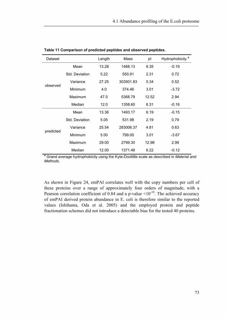
4.1 Abundance profiling of the E.coli proteome
73
Table 11 Comparison of predicted peptides and observed peptides.
Dataset Length Mass pI Hydrophobicity a
observed
Mean 13.28 1468.13 6.35 -0.19
Std. Deviation 5.22 550.91 2.31 0.72
Variance 27.25 303501.83 5.34 0.52
Minimum 4.0 374.46 3.01 -3.72
Maximum 47.0 5368.79 12.52 2.94
Median 12.0 1358.60 6.31 -0.16
predicted
Mean 13.36 1493.17 6.19 -0.15
Std. Deviation 5.05 531.98 2.19 0.79
Variance 25.54 283006.37 4.81 0.63
Minimum 5.00 799.00 3.01 -3.67
Maximum 29.00 2799.30 12.98 2.99
Median 12.00 1371.48 6.22 -0.12 a Grand average hydrophobicity using the Kyte-Doolittle scale as described in Material and Methods.
As shown in Figure 24, emPAI correlates well with the copy numbers per cell of these proteins over a range of approximately four orders of magnitude, with a Pearson correlation coefficient of 0.84 and a p-value <10-10. The achieved accuracy of emPAI derived protein abundance in E. coli is therefore similar to the reported values (Ishihama, Oda et al. 2005) and the employed protein and peptide fractionation schemes did not introduce a detectable bias for the tested 40 proteins.
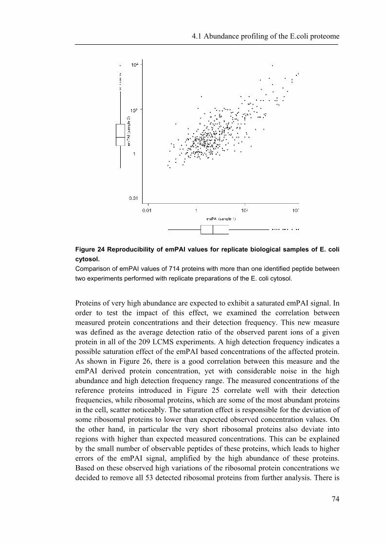
4.1 Abundance profiling of the E.coli proteome
74
Figure 24 Reproducibility of emPAI values for replicate biological samples of E. coli cytosol. Comparison of emPAI values of 714 proteins with more than one identified peptide between two experiments performed with replicate preparations of the E. coli cytosol.
Proteins of very high abundance are expected to exhibit a saturated emPAI signal. In order to test the impact of this effect, we examined the correlation between measured protein concentrations and their detection frequency. This new measure was defined as the average detection ratio of the observed parent ions of a given protein in all of the 209 LCMS experiments. A high detection frequency indicates a possible saturation effect of the emPAI based concentrations of the affected protein. As shown in Figure 26, there is a good correlation between this measure and the emPAI derived protein concentration, yet with considerable noise in the high abundance and high detection frequency range. The measured concentrations of the reference proteins introduced in Figure 25 correlate well with their detection frequencies, while ribosomal proteins, which are some of the most abundant proteins in the cell, scatter noticeably. The saturation effect is responsible for the deviation of some ribosomal proteins to lower than expected observed concentration values. On the other hand, in particular the very short ribosomal proteins also deviate into regions with higher than expected measured concentrations. This can be explained by the small number of observable peptides of these proteins, which leads to higher errors of the emPAI signal, amplified by the high abundance of these proteins. Based on these observed high variations of the ribosomal protein concentrations we decided to remove all 53 detected ribosomal proteins from further analysis. There is

4.1 Abundance profiling of the E.coli proteome
75
a general tendency of other high abundance proteins and small proteins to exhibit emPAI concentrations of limited accuracy, but removal of all these proteins would inevitably lead to other artifacts in the following analysis. We therefore decided to keep these proteins and accept the noise they are introducing.
Figure 25 Correlation between observed emPAI values and independently measured protein copy numbers per cell. Protein abundances in the E. coli cytosol as measured by the emPAI approach correlate well with protein copy numbers per cell measured independently by isotope dilution using spiked E. coli BW25113 cells containing 40 proteins with known amounts (Ishii, Nakahigashi et al. 2007). A dynamic range of approximately 4 orders of magnitude of protein copy numbers per cell is covered. The Pearson correlation coefficient is 0.84 with a p-value < 10-10 for logarithmized and 0.52 (p-value <10-4) for non-logarithmized variables.
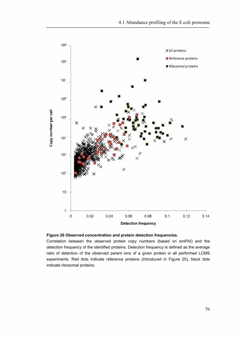
4.1 Abundance profiling of the E.coli proteome
76
Figure 26 Observed concentration and protein detection frequencies. Correlation between the observed protein copy numbers (based on emPAI) and the detection frequency of the identified proteins. Detection frequency is defined as the average ratio of detection of the observed parent ions of a given protein in all performed LCMS experiments. Red dots indicate reference proteins (introduced in Figure 25), black dots indicate ribosomal proteins.
4.1 Abundance profiling of the E.coli proteome
77
Coverage of abundance measurements
In order to assess the coverage of our abundance measurements we compared the final set of 1050 proteins with a set of E. coli proteins known or predicted to be cytosolic. As shown in Table 10, the ratio of uniquely detected cytosolic proteins depends on the definition of this theoretical cytosol. As described in Materials and Methods we combined experimental localization data (Lopez-Campistrous, Semchuk et al. 2005) with data from the PSORT database (Gardy, Laird et al. 2005; Rey, Acab et al. 2005) and computational transmembrane segment predictions. Our cytosol definition – shown in the last row of Table 10– results in 2680 theoretic cytosolic proteins that represent 62.5 % of the complete E. coli proteome. Applying the same strict criteria to the measured samples, 853 of the 1050 identified proteins (81.2%) can be safely considered cytosolic proteins. Under these very conservative assumptions we cover at least 32% (853 of 2680) of the theoretical E. coli cytosol. If, however, we extrapolate the experimental localization data we would cover ~75% (279 of 370) of the theoretical cytosol. Although the number of detected unique proteins that we do not consider as cytosolic is relatively high - 197 out of 1050, or 18.7% - their emPAI derived abundances indicate that these proteins represent only less than 5.4% of all measured protein copies in our sample. If the ribosomal proteins were not excluded, the amount of protein copies of non-cytosolic proteins would be less than 0.1%. This demonstrates the high specificity of our sample preparation and almost all proteins in the sample by mass can be considered cytosolic. Our method is highly sensitive in identifying and quantifying proteins even if they occur only in very low copy numbers. We were able to identify many proteins which are present in low copy number and are hardly detectable by other techniques. For example, the adenylyl protein glnE and members of the fts-family are known to be constitutively expressed at a very low level (van Heeswijk, Rabenberg et al. 1993; Errington, Daniel et al. 2003). Overall, the abundance measurements for 1050 E. coli proteins presented in this work represent the most complete study of protein abundance in a bacterial cell so far, accounting for around one fourth of all E. coli gene products with a specificity of nearly 100% for the targeted cytosolic protein set.
General characteristics of protein abundance in the E. coli cell
The main bulk of E. coli proteins in the cytosolic lysate are found in relatively small amounts, with 75% and 25% of them appearing in copy numbers below 250 and 1160, respectively (Figure 27). At the same time, a sizeable fraction of highly abundant proteins with copy numbers of up to 105 and more was identified. This broad dynamic range of abundance values corresponds to protein copy numbers per cell from ~100 to 105 and is in accordance with previously reported data on yeast in which the number of molecules per cell ranges from 50 to 106 (Ghaemmaghami, Huh et al. 2003). Both E. coli and yeast proteins show an extreme value distribution,
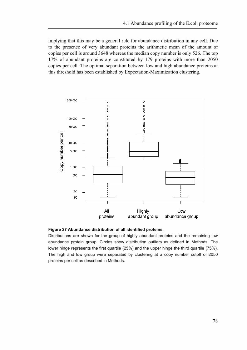
4.1 Abundance profiling of the E.coli proteome
78
implying that this may be a general rule for abundance distribution in any cell. Due to the presence of very abundant proteins the arithmetic mean of the amount of copies per cell is around 3648 whereas the median copy number is only 526. The top 17% of abundant proteins are constituted by 179 proteins with more than 2050 copies per cell. The optimal separation between low and high abundance proteins at this threshold has been established by Expectation-Maximization clustering.
Figure 27 Abundance distribution of all identified proteins. Distributions are shown for the group of highly abundant proteins and the remaining low abundance protein group. Circles show distribution outliers as defined in Methods. The lower hinge represents the first quartile (25%) and the upper hinge the third quartile (75%). The high and low group were separated by clustering at a copy number cutoff of 2050 proteins per cell as described in Methods.
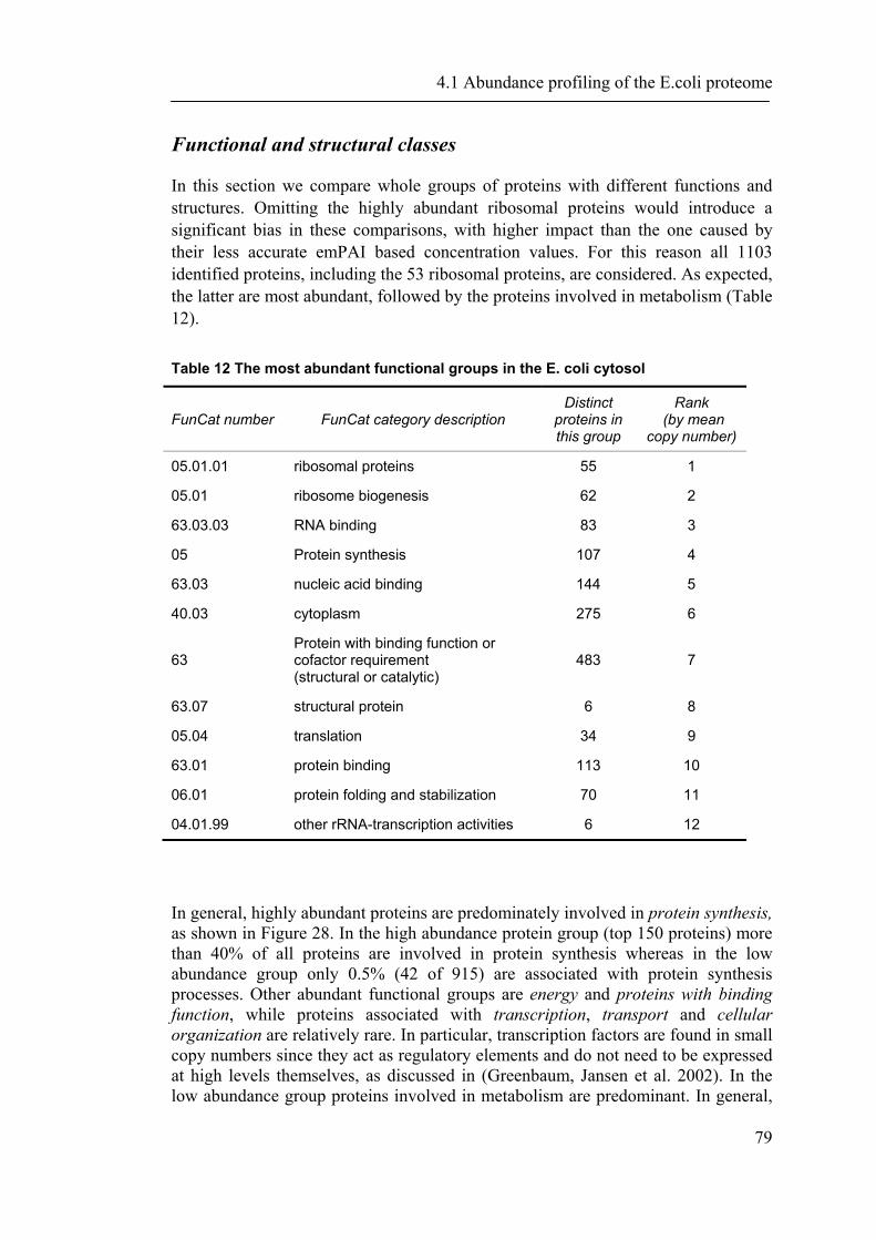
4.1 Abundance profiling of the E.coli proteome
79
Functional and structural classes
In this section we compare whole groups of proteins with different functions and structures. Omitting the highly abundant ribosomal proteins would introduce a significant bias in these comparisons, with higher impact than the one caused by their less accurate emPAI based concentration values. For this reason all 1103 identified proteins, including the 53 ribosomal proteins, are considered. As expected, the latter are most abundant, followed by the proteins involved in metabolism (Table 12).
Table 12 The most abundant functional groups in the E. coli cytosol
FunCat number FunCat category description Distinct
proteins in this group
Rank (by mean
copy number)
05.01.01 ribosomal proteins 55 1
05.01 ribosome biogenesis 62 2
63.03.03 RNA binding 83 3
05 Protein synthesis 107 4
63.03 nucleic acid binding 144 5
40.03 cytoplasm 275 6
63 Protein with binding function or cofactor requirement (structural or catalytic)
483 7
63.07 structural protein 6 8
05.04 translation 34 9
63.01 protein binding 113 10
06.01 protein folding and stabilization 70 11
04.01.99 other rRNA-transcription activities 6 12
In general, highly abundant proteins are predominately involved in protein synthesis, as shown in Figure 28. In the high abundance protein group (top 150 proteins) more than 40% of all proteins are involved in protein synthesis whereas in the low abundance group only 0.5% (42 of 915) are associated with protein synthesis processes. Other abundant functional groups are energy and proteins with binding function, while proteins associated with transcription, transport and cellular organization are relatively rare. In particular, transcription factors are found in small copy numbers since they act as regulatory elements and do not need to be expressed at high levels themselves, as discussed in (Greenbaum, Jansen et al. 2002). In the low abundance group proteins involved in metabolism are predominant. In general,
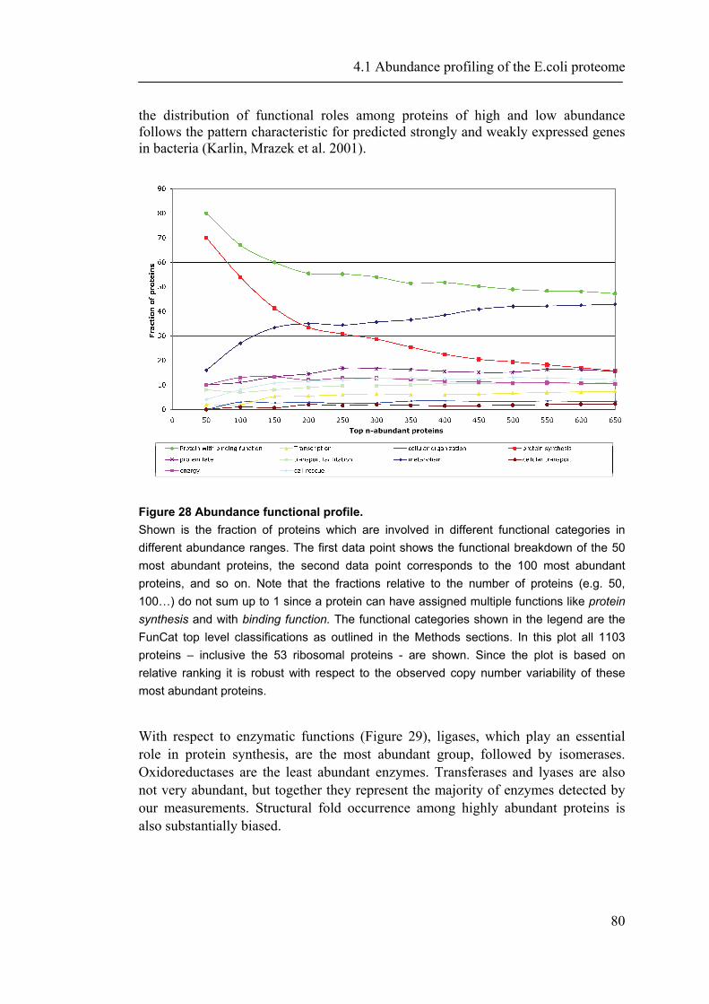
4.1 Abundance profiling of the E.coli proteome
80
the distribution of functional roles among proteins of high and low abundance follows the pattern characteristic for predicted strongly and weakly expressed genes in bacteria (Karlin, Mrazek et al. 2001).
Figure 28 Abundance functional profile. Shown is the fraction of proteins which are involved in different functional categories in different abundance ranges. The first data point shows the functional breakdown of the 50 most abundant proteins, the second data point corresponds to the 100 most abundant proteins, and so on. Note that the fractions relative to the number of proteins (e.g. 50, 100…) do not sum up to 1 since a protein can have assigned multiple functions like protein synthesis and with binding function. The functional categories shown in the legend are the FunCat top level classifications as outlined in the Methods sections. In this plot all 1103 proteins – inclusive the 53 ribosomal proteins - are shown. Since the plot is based on relative ranking it is robust with respect to the observed copy number variability of these most abundant proteins.
With respect to enzymatic functions (Figure 29), ligases, which play an essential role in protein synthesis, are the most abundant group, followed by isomerases. Oxidoreductases are the least abundant enzymes. Transferases and lyases are also not very abundant, but together they represent the majority of enzymes detected by our measurements. Structural fold occurrence among highly abundant proteins is also substantially biased.
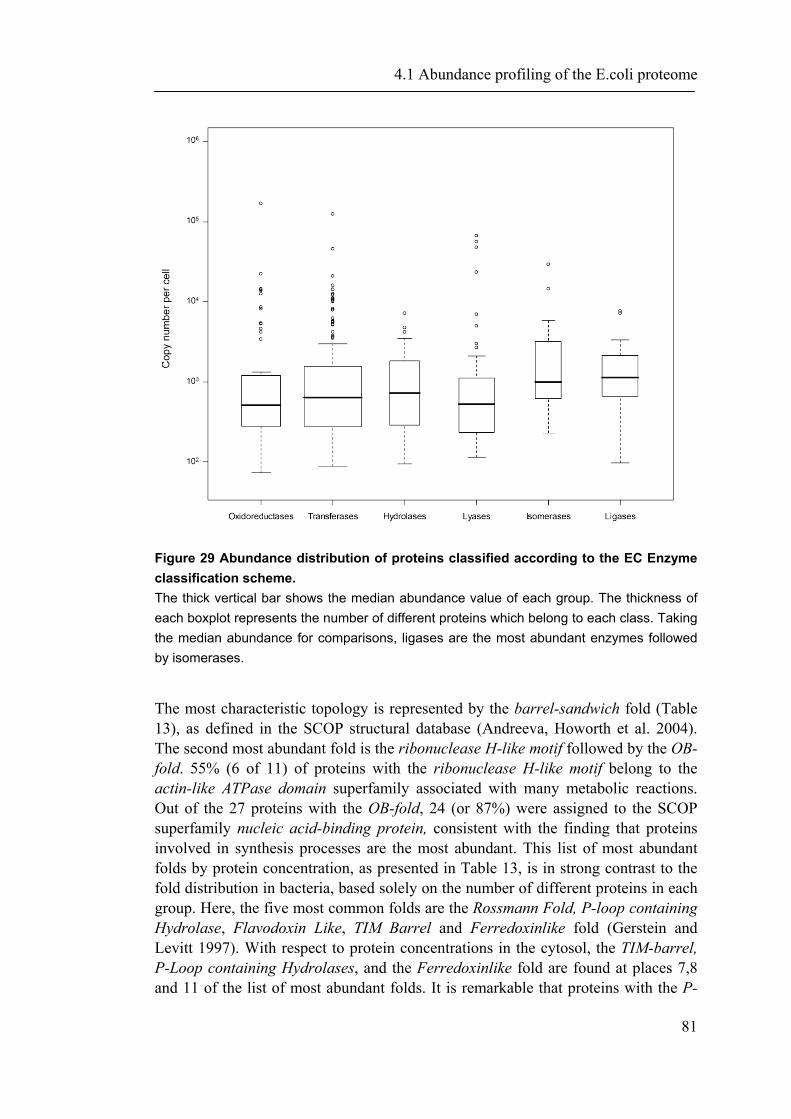
4.1 Abundance profiling of the E.coli proteome
81
Figure 29 Abundance distribution of proteins classified according to the EC Enzyme classification scheme. The thick vertical bar shows the median abundance value of each group. The thickness of each boxplot represents the number of different proteins which belong to each class. Taking the median abundance for comparisons, ligases are the most abundant enzymes followed by isomerases.
The most characteristic topology is represented by the barrel-sandwich fold (Table 13), as defined in the SCOP structural database (Andreeva, Howorth et al. 2004). The second most abundant fold is the ribonuclease H-like motif followed by the OB-fold. 55% (6 of 11) of proteins with the ribonuclease H-like motif belong to the actin-like ATPase domain superfamily associated with many metabolic reactions. Out of the 27 proteins with the OB-fold, 24 (or 87%) were assigned to the SCOP superfamily nucleic acid-binding protein, consistent with the finding that proteins involved in synthesis processes are the most abundant. This list of most abundant folds by protein concentration, as presented in Table 13, is in strong contrast to the fold distribution in bacteria, based solely on the number of different proteins in each group. Here, the five most common folds are the Rossmann Fold, P-loop containing Hydrolase, Flavodoxin Like, TIM Barrel and Ferredoxinlike fold (Gerstein and Levitt 1997). With respect to protein concentrations in the cytosol, the TIM-barrel, P-Loop containing Hydrolases, and the Ferredoxinlike fold are found at places 7,8 and 11 of the list of most abundant folds. It is remarkable that proteins with the P-
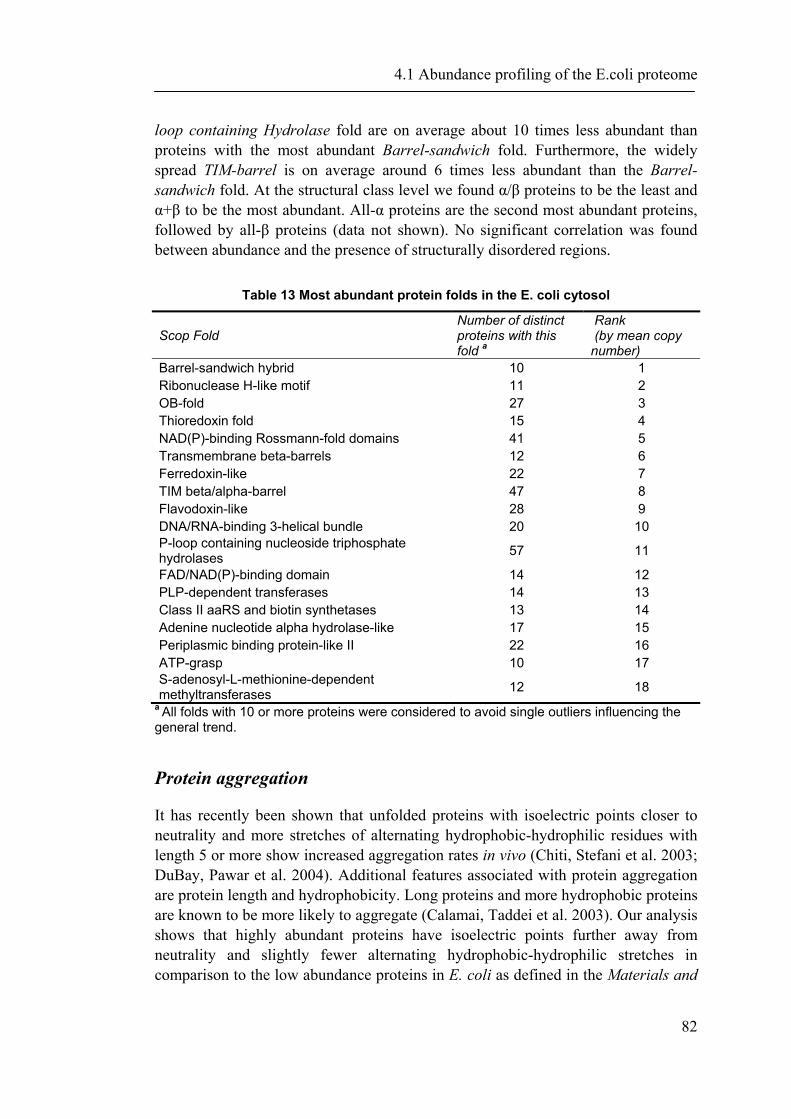
4.1 Abundance profiling of the E.coli proteome
82
loop containing Hydrolase fold are on average about 10 times less abundant than proteins with the most abundant Barrel-sandwich fold. Furthermore, the widely spread TIM-barrel is on average around 6 times less abundant than the Barrel-sandwich fold. At the structural class level we found α/β proteins to be the least and α+β to be the most abundant. All-α proteins are the second most abundant proteins, followed by all-β proteins (data not shown). No significant correlation was found between abundance and the presence of structurally disordered regions.
Table 13 Most abundant protein folds in the E. coli cytosol
Scop Fold Number of distinct proteins with this fold a
Rank (by mean copy number)
Barrel-sandwich hybrid 10 1 Ribonuclease H-like motif 11 2 OB-fold 27 3 Thioredoxin fold 15 4 NAD(P)-binding Rossmann-fold domains 41 5 Transmembrane beta-barrels 12 6 Ferredoxin-like 22 7 TIM beta/alpha-barrel 47 8 Flavodoxin-like 28 9 DNA/RNA-binding 3-helical bundle 20 10 P-loop containing nucleoside triphosphate hydrolases 57 11
FAD/NAD(P)-binding domain 14 12 PLP-dependent transferases 14 13 Class II aaRS and biotin synthetases 13 14 Adenine nucleotide alpha hydrolase-like 17 15 Periplasmic binding protein-like II 22 16 ATP-grasp 10 17 S-adenosyl-L-methionine-dependent methyltransferases 12 18
a All folds with 10 or more proteins were considered to avoid single outliers influencing the general trend.
Protein aggregation
It has recently been shown that unfolded proteins with isoelectric points closer to neutrality and more stretches of alternating hydrophobic-hydrophilic residues with length 5 or more show increased aggregation rates in vivo (Chiti, Stefani et al. 2003; DuBay, Pawar et al. 2004). Additional features associated with protein aggregation are protein length and hydrophobicity. Long proteins and more hydrophobic proteins are known to be more likely to aggregate (Calamai, Taddei et al. 2003). Our analysis shows that highly abundant proteins have isoelectric points further away from neutrality and slightly fewer alternating hydrophobic-hydrophilic stretches in comparison to the low abundance proteins in E. coli as defined in the Materials and

4.1 Abundance profiling of the E.coli proteome
83
Methods section. Additionally we show that highly abundant proteins are on average shorter and less hydrophobic than proteins with low copy numbers (Table 14). Taken together, our data indicate that highly abundant proteins may have evolved to be less prone to aggregation. These observations are further strengthened when ribosomal proteins, known to be highly expressed, are also considered.
Table 14 Comparison of features associated with protein aggregation between high abundant proteins and the remaining detected proteins. The high abundant group is defined as described in Material and Methods.
Property Low abundant
proteins Mean (Median)
High abundant proteins
Mean (Median)
P-value KS-, MW-test
Protein length (in amino acids) 386 (327) 309 (252) 10-6, 10-7
Number of alternating hydrophobic-/hydrophilic stretches (>= 5aa)
11.7 (9.0) 9.5 (8.0) 0.03, 10-4
pI distance from neutrality 1.52 (1.50) 1.69 (1,84) 0.003, 0.01
Hydrophobicity (Kyte-Doolite scale) -0.20 (-0.21) -0.25 (-0.24) 0.17, 0.08
Amino acid composition
In agreement with Greenbaum et al. (2002), greater frequencies of small amino acids Ala, Gly and Val were found in highly abundant proteins. Additionally we determined that Leu, Gln, Pro, Ser and Trp are more common in low abundance proteins whereas Lys and Glu is more common in the high abundance group. These compositional differences are a direct consequence of the functional bias observed in abundant and scarce proteins, as described above. Amino acid preferences in proteins of different functionality have been utilized before for coarse function prediction from sequence alone (e.g. (Cai, Han et al. 2003)).
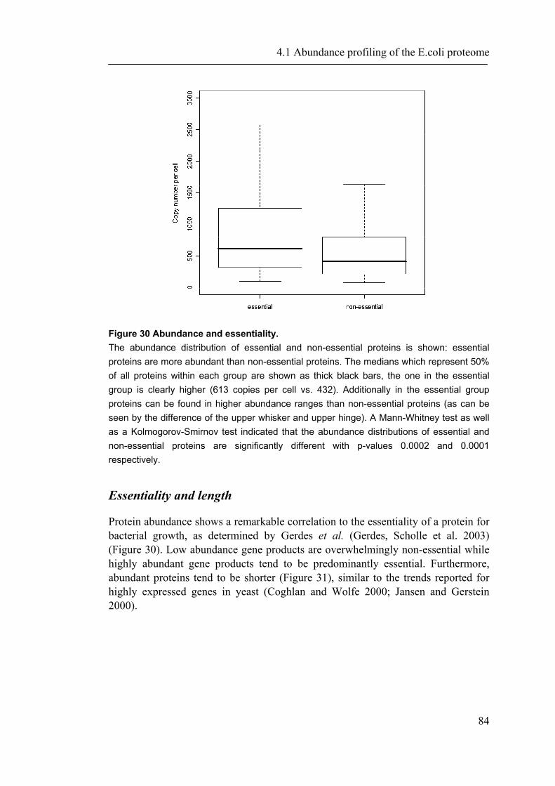
4.1 Abundance profiling of the E.coli proteome
84
Figure 30 Abundance and essentiality. The abundance distribution of essential and non-essential proteins is shown: essential proteins are more abundant than non-essential proteins. The medians which represent 50% of all proteins within each group are shown as thick black bars, the one in the essential group is clearly higher (613 copies per cell vs. 432). Additionally in the essential group proteins can be found in higher abundance ranges than non-essential proteins (as can be seen by the difference of the upper whisker and upper hinge). A Mann-Whitney test as well as a Kolmogorov-Smirnov test indicated that the abundance distributions of essential and non-essential proteins are significantly different with p-values 0.0002 and 0.0001 respectively.
Essentiality and length
Protein abundance shows a remarkable correlation to the essentiality of a protein for bacterial growth, as determined by Gerdes et al. (Gerdes, Scholle et al. 2003) (Figure 30). Low abundance gene products are overwhelmingly non-essential while highly abundant gene products tend to be predominantly essential. Furthermore, abundant proteins tend to be shorter (Figure 31), similar to the trends reported for highly expressed genes in yeast (Coghlan and Wolfe 2000; Jansen and Gerstein 2000).
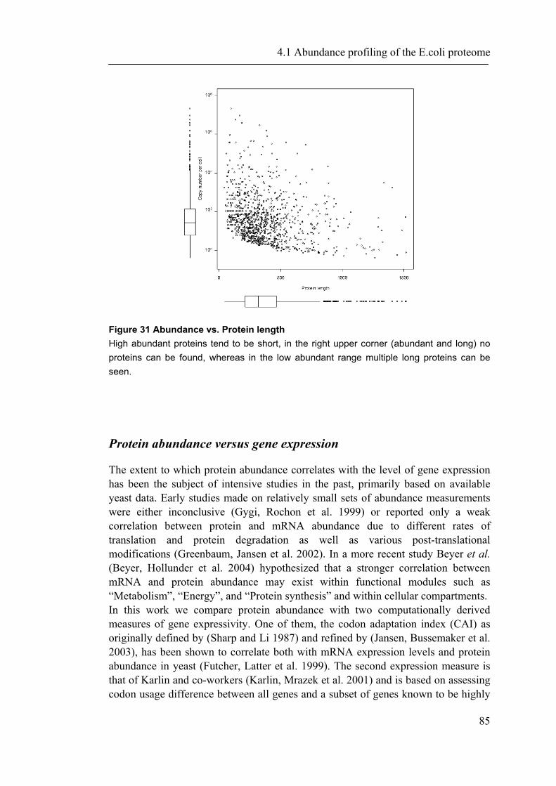
4.1 Abundance profiling of the E.coli proteome
85
Figure 31 Abundance vs. Protein length High abundant proteins tend to be short, in the right upper corner (abundant and long) no proteins can be found, whereas in the low abundant range multiple long proteins can be seen.
Protein abundance versus gene expression
The extent to which protein abundance correlates with the level of gene expression has been the subject of intensive studies in the past, primarily based on available yeast data. Early studies made on relatively small sets of abundance measurements were either inconclusive (Gygi, Rochon et al. 1999) or reported only a weak correlation between protein and mRNA abundance due to different rates of translation and protein degradation as well as various post-translational modifications (Greenbaum, Jansen et al. 2002). In a more recent study Beyer et al. (Beyer, Hollunder et al. 2004) hypothesized that a stronger correlation between mRNA and protein abundance may exist within functional modules such as “Metabolism”, “Energy”, and “Protein synthesis” and within cellular compartments. In this work we compare protein abundance with two computationally derived measures of gene expressivity. One of them, the codon adaptation index (CAI) as originally defined by (Sharp and Li 1987) and refined by (Jansen, Bussemaker et al. 2003), has been shown to correlate both with mRNA expression levels and protein abundance in yeast (Futcher, Latter et al. 1999). The second expression measure is that of Karlin and co-workers (Karlin, Mrazek et al. 2001) and is based on assessing codon usage difference between all genes and a subset of genes known to be highly
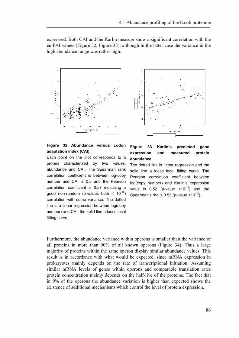
4.1 Abundance profiling of the E.coli proteome
86
expressed. Both CAI and the Karlin measure show a significant correlation with the emPAI values (Figure 32, Figure 33), although in the latter case the variance in the high abundance range was rather high.
Figure 32 Abundance versus codon adaptation index (CAI). Each point on the plot corresponds to a protein characterized by two values: abundance and CAI. The Spearman rank correlation coefficient rs between log-copy number and CAI is 0.5 and the Pearson correlation coefficient is 0.57 indicating a good non-random (p-values both < 10-16) correlation with some variance. The dotted line is a linear regression between log(copy number) and CAI, the solid line a loess local fitting curve.
Figure 33 Karlin’s predicted gene expression and measured protein abundance. The dotted line is linear regression and the solid line a loess local fitting curve. The Pearson correlation coefficient between log(copy number) and Karlin’s expression value is 0.52 (p-value <10-12) and the Spearman’s rho is 0.53 (p-value <10-12).
Furthermore, the abundance variance within operons is smaller than the variance of all proteins in more than 90% of all known operons (Figure 34). Thus a large majority of proteins within the same operon display similar abundance values. This result is in accordance with what would be expected, since mRNA expression in prokaryotes mainly depends on the rate of transcriptional initiation. Assuming similar mRNA levels of genes within operons and comparable translation rates protein concentration mainly depends on the half-live of the proteins. The fact that in 9% of the operons the abundance variation is higher than expected shows the existence of additional mechanisms which control the level of protein expression.
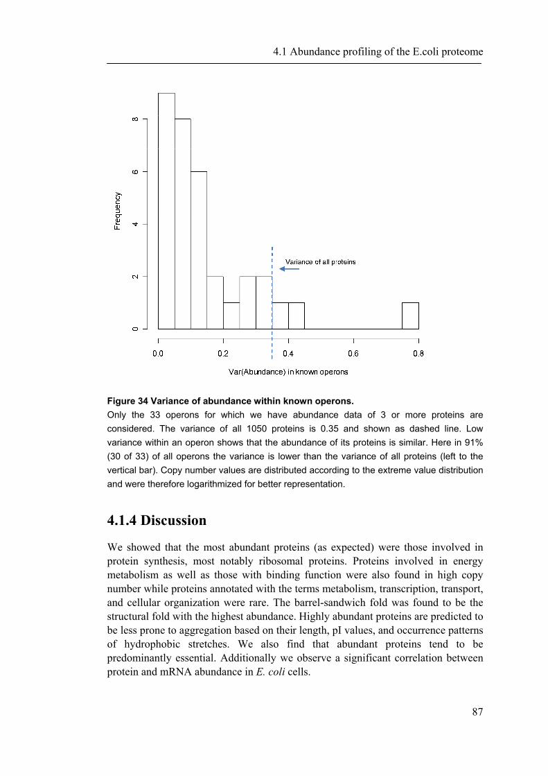
4.1 Abundance profiling of the E.coli proteome
87
Figure 34 Variance of abundance within known operons. Only the 33 operons for which we have abundance data of 3 or more proteins are considered. The variance of all 1050 proteins is 0.35 and shown as dashed line. Low variance within an operon shows that the abundance of its proteins is similar. Here in 91% (30 of 33) of all operons the variance is lower than the variance of all proteins (left to the vertical bar). Copy number values are distributed according to the extreme value distribution and were therefore logarithmized for better representation.
4.1.4 Discussion
We showed that the most abundant proteins (as expected) were those involved in protein synthesis, most notably ribosomal proteins. Proteins involved in energy metabolism as well as those with binding function were also found in high copy number while proteins annotated with the terms metabolism, transcription, transport, and cellular organization were rare. The barrel-sandwich fold was found to be the structural fold with the highest abundance. Highly abundant proteins are predicted to be less prone to aggregation based on their length, pI values, and occurrence patterns of hydrophobic stretches. We also find that abundant proteins tend to be predominantly essential. Additionally we observe a significant correlation between protein and mRNA abundance in E. coli cells.
4.2 Genome architectures and evaluation
88
4.2 Genome architectures and evaluation
In the previous section we analyzed absolute quantities of the E.coli proteome. As next step we further questioned the impact of underlying genome structures. It was reported in various studies that the GC content of genes influences gene expression (Kudla, Lipinski et al. 2006). However, in contrast to bacteria, higher mammalian genomes do not have “one GC content”, but are build up of large regions with fairly homogenous GC content widely known as isochores. In the following section we investigate such higher genome attributes at large-scale and present a new consensus method for fully automated isochore assignment. We show that our new method provides superior explanation of experimental observations than previous approaches. Finally, we present a rich online resource and database for exploration and download of all data.
4.2.1 Introduction
More than three decades ago gradient density analyses of fragmented DNA identified long compositionally homogenous regions on mammalian chromosomes, widely known as isochores (Filipski, Thiery et al. 1973; Macaya, Thiery et al. 1976; Thiery, Macaya et al. 1976) or long homogeneous genome regions (LHGRs) (Oliver, Carpena et al. 2002), associated with a wide range of important biological properties. Gene density is up to 16 times higher in GC-rich isochores than in GC-poor isochores (Mouchiroud, D'Onofrio et al. 1991), and the genes in the high GC-isochores code for shorter proteins and are more compact with a smaller amount of introns (Duret, Mouchiroud et al. 1995). It was also shown that the GC-rich codons, such as those coding for alanine and arginine, are more frequent in GC-rich isochores (D'Onofrio, Mouchiroud et al. 1991; Clay, Caccio et al. 1996). The distribution of repeat elements is influenced by the isochore structure of the genome: SINE (short-interspersed nuclear element) sequences tend to be more frequent in GC-rich isochores while the LINE (long-interspersed nuclear elements) sequences are preferentially found in GC-poorer regions (Meunier-Rotival, Soriano et al. 1982; Soriano, Meunier-Rotival et al. 1983; Jabbari and Bernardi 1998). The structure of chromosome bands also correlates with isochores: T-bands predominantly consist of GC-rich isochores, while the GC-poorer isochores are found in G-bands (Saccone, De Sario et al. 1992; Saccone, De Sario et al. 1993; Costantini, Clay et al. 2006). The recombination frequency is higher (Eisenbarth, Beyer et al. 2000; Fullerton, Bernardo Carvalho et al. 2001) and the replication starts up to 2 hours earlier (Tenzen, Yamagata et al. 1997) in regions with high GC-content. Further progress in understanding the biological role and evolution of long-range variation in base composition is seriously hindered by the lack of objective and
4.2 Genome architectures and evaluation
89
generally accepted isochore assignment methods. A multitude of prediction approaches has been developed by various groups (Ramensky, Makeev et al. 2001; Zhang, Wang et al. 2001; Oliver, Carpena et al. 2004; Zhang, Gao et al. 2005; Costantini, Clay et al. 2006; Haiminen and Mannila 2007), but no single resource allows to access, compare, and combine isochore assignments made by various techniques in different genomes. Here we introduce a new consensus predictor which characterizes the level of support for isochore locations determined by individual methods. We present a database of isochore maps for all completely sequenced vertebrate genomes and interactive viewers that allow to explore this “fundamental level of genome organization” (Eyre-Walker and Hurst 2001) online (http://webclu.bio.wzw.tum.de/isobase).
4.2.2 Material and Methods
Isochore assignments
We refer to the isochore nomenclature as it was first described based on ultra-centrifugation experiments (Bernardi 1989). Bernardi and colleagues defined the isochores according to their GC-content (Costantini, Clay et al. 2006). There are three isochore types with high GC-content: H3 (> 53%), H2 (46% - 53%), H1 (41% - 46%), and two types with low GC-content: L1 (< 37%) and L2 (37% - 41%). The Bernardi group (Costantini, Clay et al. 2006) calculated the GC-content of 100 kb long, non-overlapping sequence windows and then merged the windows if the difference in their GC content was below 1-2%. However, no hard threshold was used, and in many cases subjective decisions were made whether or not to merge windows, making the Constantini method as described in the original publication hardly fully-automatable. In particular, this circumstance makes it impossible to consider the Constantini data for our comparison of isochore assignment methods which is based on a more recent version of the human genome than the one used in the original publication. In this work isochores were predicted by four methods for automatic genome segmentation: GC-Profile (Zhang, Wang et al. 2001; Zhang, Gao et al. 2005), BASIO (Ramensky, Makeev et al. 2001), IsoFinder (Oliver, Carpena et al. 2004), and least squares optimal segmentation (Haiminen and Mannila 2007). Briefly, GC-Profile is a windowless method which recursively partitions the input sequence into two subsequences, left and right, based on the quadratic divergence between statistical measures (such as genome order indices, a2+c2+g2+t2, where a, c, g, and t are occurrences of individual bases) reflecting base composition. IsoFinder moves a sliding pointer along the input DNA sequence and finds a position that maximizes the GC difference between its left and right portions according to the t-Student statistics. Then both portions get split into non-overlapping 300 kb windows, and for

4.2 Genome architectures and evaluation
90
each individual window the GC content is computed. If the mean values of the window GC content on the left and on the right from the pointer position are significantly different, this position becomes the cutting point and the input sequence gets divided into two subsequences. Both GC-Profile and IsoFinder proceed from left to right and may produce different results if the direction is inverted. BASIO calculates Bayesian marginal likelihood for sequence segments and, for reasonably short DNA contigs, attempts to find a global maximum of the overall likelihood over all possible configurations of segment borders using a Viterbi-like dynamic programming algorithm. For large DNA sequences, such as complete chromosomes, BASIO relies on an approximate split-and-merge procedure to find an optimal segmentation. We applied the BASIO method using the default border insertion penalty 3 and 10 kb sequence blocks as initial input. Finally, the Least Squares method calculates GC content in non-overlapping 100 kb windows and then derives optimal segmentation of the resulting array of real values which yields the minimal sum of squares of the Euclidian distance between each value and its segment average. However, the Least Squares algorithm requires the user to provide the expected number of output segments as a parameter. As an estimate of this number for the Least-Squares method we utilized the minimum number of isochores produced by the three other methods - GC-Profile, BASIO, and IsoFinder. This approach makes over-fragmentation unlikely and provides a lower limit for the actual number of isochores. Methods that rely on any information beyond the raw nucleotide sequence for isochore prediction were not considered in this study. For example, the markovian approach of Melodima et al (Melodelima, Gueguen et al. 2006) incorporates information about known biological features such as genes and their properties to create hidden Markov models. By contrast, all the methods in this study are solely based on the GC content and therefore can be used even in the absence of reliable gene models, e.g. in a newly sequenced genome.
Genomic data
We used the human genome as a test case for comparing isochore assignments made by different methods. The latest human genome assembly hg18 (build 36) was obtained from the UCSC genome browser (Karolchik, Kuhn et al. 2008). Further vertebrate genomes were downloaded from UCSC, Ensembl (Flicek, Aken et al. 2008), and the Broad Institute (www.broad.mit.edu) (Mikkelsen, Wakefield et al. 2007). Assembly parts marked as random and short scaffold parts were not considered. The UCSC known genes models were used (Hsu, Kent et al. 2006) for computing the gene density defined as the number of genes per million nucleotides (Mb). To determine the gene density in individual isochores we counted the number of genes that start in each isochore family and divided it by the total amount of genomic DNA classified into the respective isochore family. For the regression
4.2 Genome architectures and evaluation
91
analysis the isochore family lables were translated into their ordinal value: from 1 for the L1-family to 5 for the H3 family. Gene density values were logarithmized (natural logarithm) as they grow polynominally with increasing isochore family number. Statistical tests were performed using PROMPT (Schmidt and Frishman 2006).
Entropy distance
In this study we are measuring the distance between two segmentations P and Q by the entropy distance as described by Haiminen et al. (Haiminen, Mannila et al. 2007). Briefly, the entropy H of a segmentation P with k segments can be defined as
∑=
−=k
iii ppPH
1)Pr(log)Pr()( with
sequencesegmentedtheoflengthtotal
isegmentoflengthpi =)Pr(
The entropy distance is the conditional entropy of P given Q and vice versa. Conditional entropy is thus an information theoretic measure that quantifies the amount of information that one segmentation gives about the other. The lower the entropy distance between the reference isochore segmentation and the prediction, the better is the prediction. As further shown in (Haiminen, Mannila et al. 2007) the conditional probability of the segmentation P given the segmentation Q can be computed with the complexity O(kp+kq) with kp and kq being the number of segments in P and Q. This efficient algorithm uses the fact that H(P|Q) = H(U) – H(Q), with H(U) being the entropy of the union of P and Q. Therefore, the entropy distance of P and Q can be represented as H(P|Q) + H(Q|P) = 2 H(U) – H(Q) – H(P).
Consensus isochore assignments
We sought to integrate several available methods in order to provide more balanced isochore assignments. It is known that GC fluctuations tend to be higher in GC rich regions than in GC poor regions (Clay and Bernardi 2001). This means, for example, that if one chops human DNA sequence into blocks of 100 kb, the GC content variation between such blocks in a GC-rich region will be higher than in a GC-poor region. A segmentation algorithm that aims at partitioning a genome based on the GC variance must be able to handle these differences. If a method is optimized to detect small GC jumps between genomic blocks, it is likely to overfragment GC-rich regions. Conversely, if the cut-off value of the GC content change required to initiate a new segment is too high, GC changes between different isochores in GC-poor regions will not be detected. The significant variety of currently available isochore prediction methods reflects to some degree this difficult challenge.
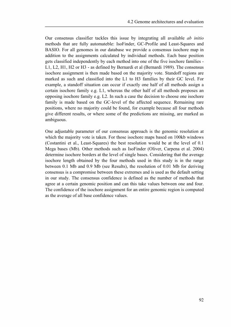
4.2 Genome architectures and evaluation
92
Our consensus classifier tackles this issue by integrating all available ab initio methods that are fully automateble: IsoFinder, GC-Profile and Least-Squares and BASIO. For all genomes in our database we provide a consensus isochore map in addition to the assignments calculated by individual methods. Each base position gets classified independently by each method into one of the five isochore families - L1, L2, H1, H2 or H3 - as defined by Bernardi et al (Bernardi 1989). The consensus isochore assignment is then made based on the majority vote. Standoff regions are marked as such and classified into the L1 to H3 families by their GC level. For example, a standoff situation can occur if exactly one half of all methods assign a certain isochore family e.g. L1, whereas the other half of all methods proposes an opposing isochore family e.g. L2. In such a case the decision to choose one isochore family is made based on the GC-level of the affected sequence. Remaining rare positions, where no majority could be found, for example because all four methods give different results, or where some of the predictions are missing, are marked as ambiguous. One adjustable parameter of our consensus approach is the genomic resolution at which the majority vote is taken. For those isochore maps based on 100kb windows (Costantini et al., Least-Squares) the best resolution would be at the level of 0.1 Mega bases (Mb). Other methods such as IsoFinder (Oliver, Carpena et al. 2004) determine isochore borders at the level of single bases. Considering that the average isochore length obtained by the four methods used in this study is in the range between 0.1 Mb and 0.9 Mb (see Results), the resolution of 0.01 Mb for deriving consensus is a compromise between these extremes and is used as the default setting in our study. The consensus confidence is defined as the number of methods that agree at a certain genomic position and can this take values between one and four. The confidence of the isochore assignment for an entire genomic region is computed as the average of all base confidence values.
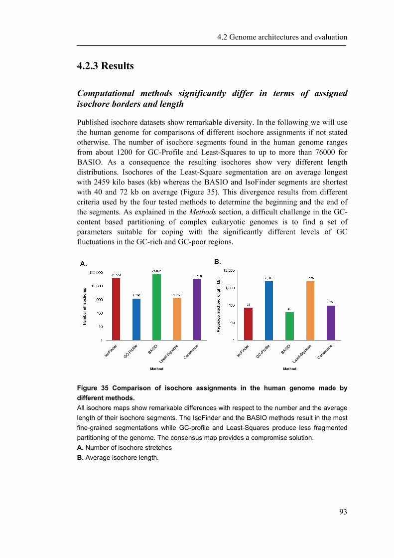
4.2 Genome architectures and evaluation
93
4.2.3 Results
Computational methods significantly differ in terms of assigned isochore borders and length
Published isochore datasets show remarkable diversity. In the following we will use the human genome for comparisons of different isochore assignments if not stated otherwise. The number of isochore segments found in the human genome ranges from about 1200 for GC-Profile and Least-Squares to up to more than 76000 for BASIO. As a consequence the resulting isochores show very different length distributions. Isochores of the Least-Square segmentation are on average longest with 2459 kilo bases (kb) whereas the BASIO and IsoFinder segments are shortest with 40 and 72 kb on average (Figure 35). This divergence results from different criteria used by the four tested methods to determine the beginning and the end of the segments. As explained in the Methods section, a difficult challenge in the GC-content based partitioning of complex eukaryotic genomes is to find a set of parameters suitable for coping with the significantly different levels of GC fluctuations in the GC-rich and GC-poor regions.
Figure 35 Comparison of isochore assignments in the human genome made by different methods. All isochore maps show remarkable differences with respect to the number and the average length of their isochore segments. The IsoFinder and the BASIO methods result in the most fine-grained segmentations while GC-profile and Least-Squares produce less fragmented partitioning of the genome. The consensus map provides a compromise solution. A. Number of isochore stretches B. Average isochore length.
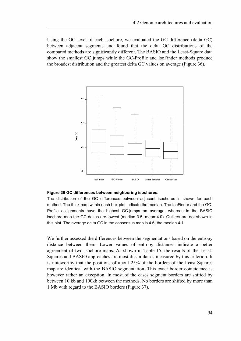
4.2 Genome architectures and evaluation
94
Using the GC level of each isochore, we evaluated the GC difference (delta GC) between adjacent segments and found that the delta GC distributions of the compared methods are significantly different. The BASIO and the Least-Square data show the smallest GC jumps while the GC-Profile and IsoFinder methods produce the broadest distribution and the greatest delta GC values on average (Figure 36).
Figure 36 GC differences between neighboring isochores. The distribution of the GC differences between adjacent isochores is shown for each method. The thick bars within each box plot indicate the median. The IsoFinder and the GC-Profile assignments have the highest GC-jumps on average, whereas in the BASIO isochore map the GC deltas are lowest (median 3.5, mean 4.0). Outliers are not shown in this plot. The average delta GC in the consensus map is 4.6, the median 4.1.
We further assessed the differences between the segmentations based on the entropy distance between them. Lower values of entropy distances indicate a better agreement of two isochore maps. As shown in Table 15, the results of the Least-Squares and BASIO approaches are most dissimilar as measured by this criterion. It is noteworthy that the positions of about 25% of the borders of the Least-Squares map are identical with the BASIO segmentation. This exact border coincidence is however rather an exception. In most of the cases segment borders are shifted by between 10 kb and 100kb between the methods. No borders are shifted by more than 1 Mb with regard to the BASIO borders (Figure 37).
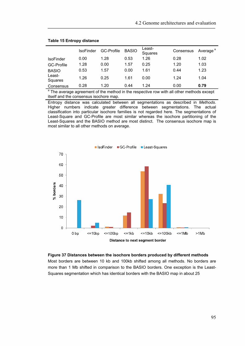
4.2 Genome architectures and evaluation
95
Table 15 Entropy distance
IsoFinder GC-Profile BASIO Least-Squares Consensus Average a
IsoFinder 0.00 1.28 0.53 1.26 0.28 1.02 GC-Profile 1.28 0.00 1.57 0.25 1.20 1.03 BASIO 0.53 1.57 0.00 1.61 0.44 1.23 Least-Squares 1.26 0.25 1.61 0.00 1.24 1.04
Consensus 0.28 1.20 0.44 1.24 0.00 0.79 a The average agreement of the method in the respective row with all other methods except itself and the consensus isochore map. Entropy distance was calculated between all segmentations as described in Methods. Higher numbers indicate greater difference between segmentations. The actual classification into particular isochore families is not regarded here. The segmentations of Least-Square and GC-Profile are most similar whereas the isochore partitioning of the Least-Squares and the BASIO method are most distinct. The consensus isochore map is most similar to all other methods on average.
Figure 37 Distances between the isochore borders produced by different methods Most borders are between 10 kb and 100kb shifted among all methods. No borders are more than 1 Mb shifted in comparison to the BASIO borders. One exception is the Least-Squares segmentation which has identical borders with the BASIO map in about 25
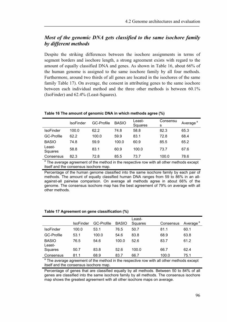
4.2 Genome architectures and evaluation
96
Most of the genomic DNA gets classified to the same isochore family by different methods
Despite the striking differences between the isochore assignments in terms of segment borders and isochore length, a strong agreement exists with regard to the amount of equally classified DNA and genes. As shown in Table 16, about 66% of the human genome is assigned to the same isochore family by all four methods. Furthermore, around two thirds of all genes are located in the isochores of the same family Table 17). On average, the consent in attributing genes to the same isochore between each individual method and the three other methods is between 60.1% (IsoFinder) and 62.4% (Least-Squares).
Table 16 The amount of genomic DNA in which methods agree (%)
IsoFinder GC-Profile BASIO Least-Squares
Consensus Average a
IsoFinder 100.0 62.2 74.8 58.8 82.3 65.3 GC-Profile 62.2 100.0 59.9 83.1 72.8 68.4 BASIO 74.8 59.9 100.0 60.9 85.5 65.2 Least-Squares 58.8 83.1 60.9 100.0 73.7 67.6
Consensus 82.3 72.8 85.5 73.7 100.0 78.6 a The average agreement of the method in the respective row with all other methods except itself and the consensus isochore map. Percentage of the human genome classified into the same isochore family by each pair of methods. The amount of equally classified human DNA ranges from 59 to 86% in an all-against-all pairwise comparison. On average all methods agree in about 66% of the genome. The consensus isochore map has the best agreement of 79% on average with all other methods.
Table 17 Agreement on gene classification (%)
IsoFinder GC-Profile BASIO Least-Squares Consensus Average a
IsoFinder 100.0 53.1 76.5 50.7 81.1 60.1 GC-Profile 53.1 100.0 54.6 83.8 68.9 63.8 BASIO 76.5 54.6 100.0 52.6 83.7 61.2 Least-Squares 50.7 83.8 52.6 100.0 66.7 62.4 Consensus 81.1 68.9 83.7 66.7 100.0 75.1 a The average agreement of the method in the respective row with all other methods except itself and the consensus isochore map. Percentage of genes that are classified equally by all methods. Between 50 to 84% of all genes are classified into the same isochore family by all methods. The consensus isochore map shows the greatest agreement with all other isochore maps on average.
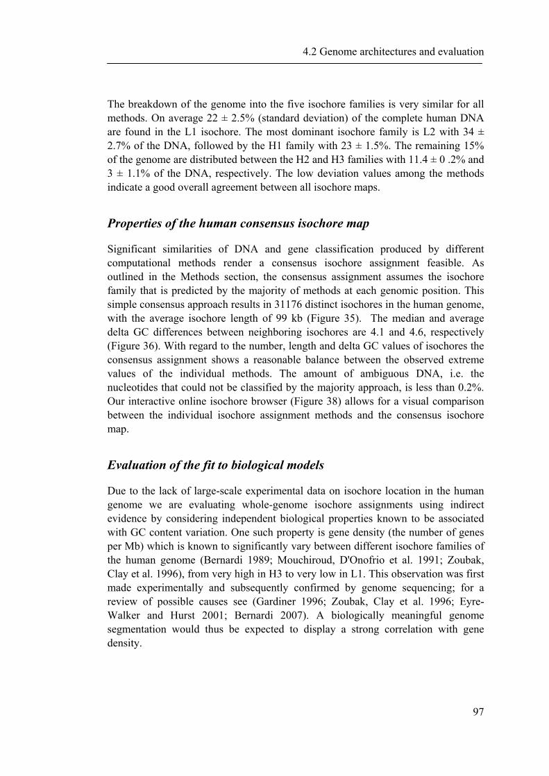
4.2 Genome architectures and evaluation
97
The breakdown of the genome into the five isochore families is very similar for all methods. On average 22 ± 2.5% (standard deviation) of the complete human DNA are found in the L1 isochore. The most dominant isochore family is L2 with 34 ± 2.7% of the DNA, followed by the H1 family with 23 ± 1.5%. The remaining 15% of the genome are distributed between the H2 and H3 families with 11.4 ± 0 .2% and 3 ± 1.1% of the DNA, respectively. The low deviation values among the methods indicate a good overall agreement between all isochore maps.
Properties of the human consensus isochore map
Significant similarities of DNA and gene classification produced by different computational methods render a consensus isochore assignment feasible. As outlined in the Methods section, the consensus assignment assumes the isochore family that is predicted by the majority of methods at each genomic position. This simple consensus approach results in 31176 distinct isochores in the human genome, with the average isochore length of 99 kb (Figure 35). The median and average delta GC differences between neighboring isochores are 4.1 and 4.6, respectively (Figure 36). With regard to the number, length and delta GC values of isochores the consensus assignment shows a reasonable balance between the observed extreme values of the individual methods. The amount of ambiguous DNA, i.e. the nucleotides that could not be classified by the majority approach, is less than 0.2%. Our interactive online isochore browser (Figure 38) allows for a visual comparison between the individual isochore assignment methods and the consensus isochore map.
Evaluation of the fit to biological models
Due to the lack of large-scale experimental data on isochore location in the human genome we are evaluating whole-genome isochore assignments using indirect evidence by considering independent biological properties known to be associated with GC content variation. One such property is gene density (the number of genes per Mb) which is known to significantly vary between different isochore families of the human genome (Bernardi 1989; Mouchiroud, D'Onofrio et al. 1991; Zoubak, Clay et al. 1996), from very high in H3 to very low in L1. This observation was first made experimentally and subsequently confirmed by genome sequencing; for a review of possible causes see (Gardiner 1996; Zoubak, Clay et al. 1996; Eyre-Walker and Hurst 2001; Bernardi 2007). A biologically meaningful genome segmentation would thus be expected to display a strong correlation with gene density.
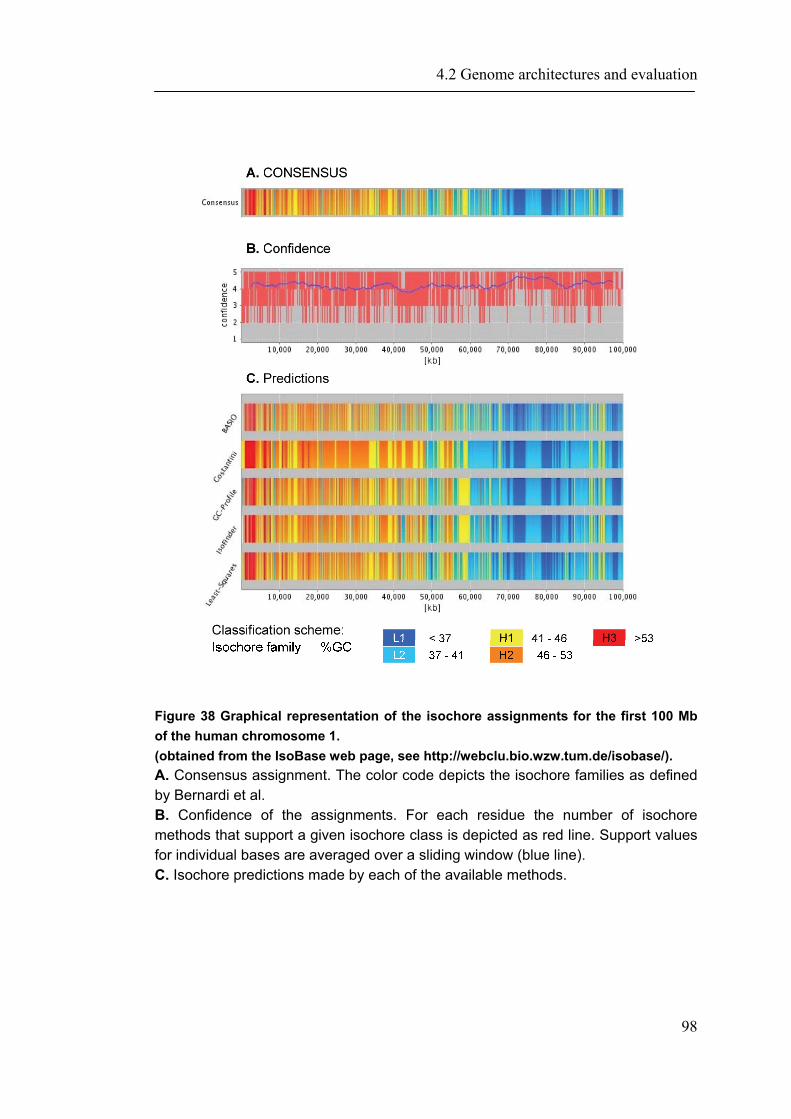
4.2 Genome architectures and evaluation
98
Figure 38 Graphical representation of the isochore assignments for the first 100 Mb of the human chromosome 1. (obtained from the IsoBase web page, see http://webclu.bio.wzw.tum.de/isobase/). A. Consensus assignment. The color code depicts the isochore families as defined by Bernardi et al. B. Confidence of the assignments. For each residue the number of isochore methods that support a given isochore class is depicted as red line. Support values for individual bases are averaged over a sliding window (blue line). C. Isochore predictions made by each of the available methods.
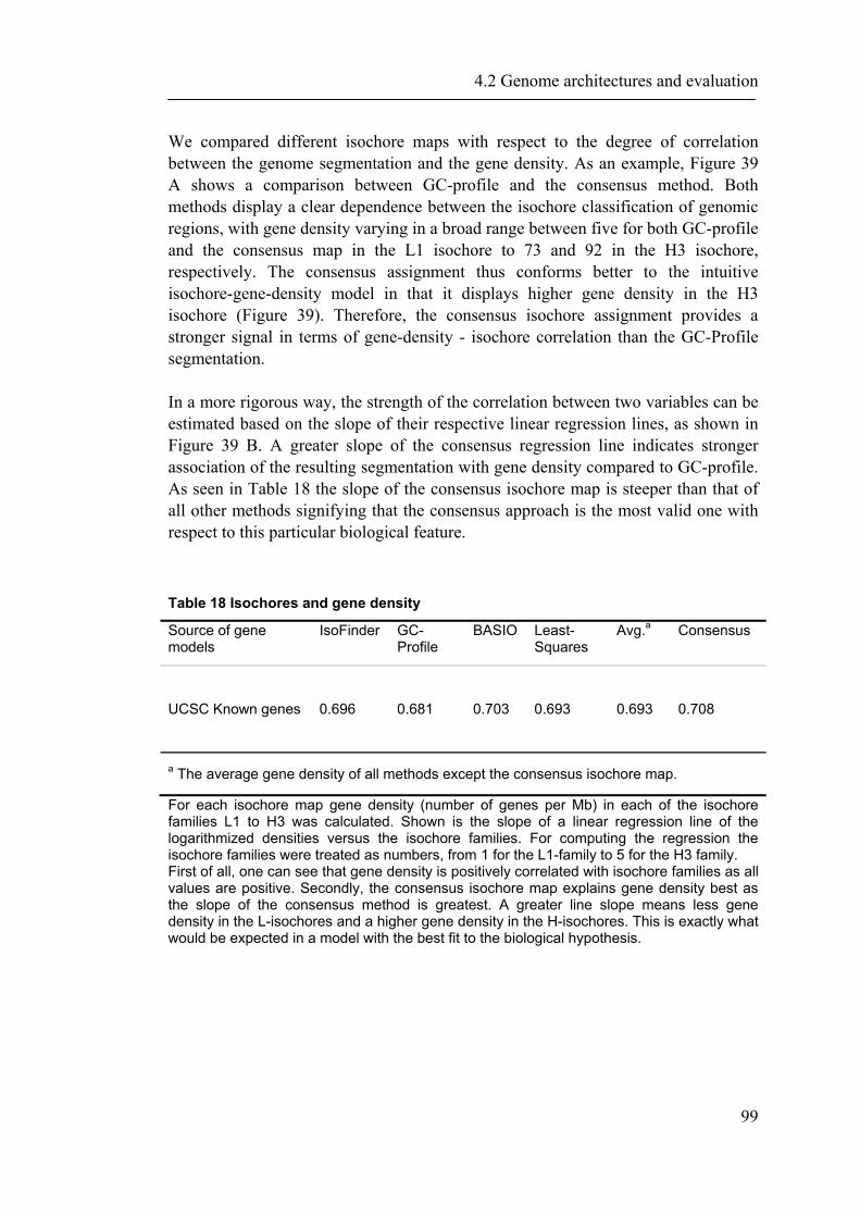
4.2 Genome architectures and evaluation
99
We compared different isochore maps with respect to the degree of correlation between the genome segmentation and the gene density. As an example, Figure 39 A shows a comparison between GC-profile and the consensus method. Both methods display a clear dependence between the isochore classification of genomic regions, with gene density varying in a broad range between five for both GC-profile and the consensus map in the L1 isochore to 73 and 92 in the H3 isochore, respectively. The consensus assignment thus conforms better to the intuitive isochore-gene-density model in that it displays higher gene density in the H3 isochore (Figure 39). Therefore, the consensus isochore assignment provides a stronger signal in terms of gene-density - isochore correlation than the GC-Profile segmentation. In a more rigorous way, the strength of the correlation between two variables can be estimated based on the slope of their respective linear regression lines, as shown in Figure 39 B. A greater slope of the consensus regression line indicates stronger association of the resulting segmentation with gene density compared to GC-profile. As seen in Table 18 the slope of the consensus isochore map is steeper than that of all other methods signifying that the consensus approach is the most valid one with respect to this particular biological feature.
Table 18 Isochores and gene density
Source of gene models
IsoFinder GC-Profile
BASIO Least-Squares
Avg.a Consensus
UCSC Known genes 0.696 0.681 0.703 0.693 0.693 0.708
a The average gene density of all methods except the consensus isochore map.
For each isochore map gene density (number of genes per Mb) in each of the isochore families L1 to H3 was calculated. Shown is the slope of a linear regression line of the logarithmized densities versus the isochore families. For computing the regression the isochore families were treated as numbers, from 1 for the L1-family to 5 for the H3 family. First of all, one can see that gene density is positively correlated with isochore families as all values are positive. Secondly, the consensus isochore map explains gene density best as the slope of the consensus method is greatest. A greater line slope means less gene density in the L-isochores and a higher gene density in the H-isochores. This is exactly what would be expected in a model with the best fit to the biological hypothesis.
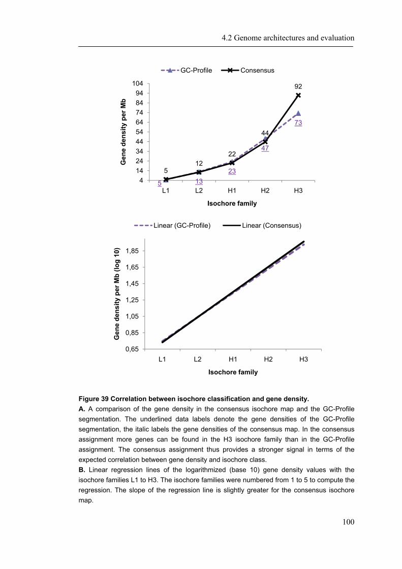
4.2 Genome architectures and evaluation
100
Figure 39 Correlation between isochore classification and gene density. A. A comparison of the gene density in the consensus isochore map and the GC-Profile segmentation. The underlined data labels denote the gene densities of the GC-Profile segmentation, the italic labels the gene densities of the consensus map. In the consensus assignment more genes can be found in the H3 isochore family than in the GC-Profile assignment. The consensus assignment thus provides a stronger signal in terms of the expected correlation between gene density and isochore class. B. Linear regression lines of the logarithmized (base 10) gene density values with the isochore families L1 to H3. The isochore families were numbered from 1 to 5 to compute the regression. The slope of the regression line is slightly greater for the consensus isochore map.
5 1323
47
73
512
22
44
92
4142434445464748494
104
L1 L2 H1 H2 H3
Gen
e de
nsity
per
Mb
Isochore family
GC-Profile Consensus
0,65
0,85
1,05
1,25
1,45
1,65
1,85
L1 L2 H1 H2 H3
Gen
e de
nsity
per
Mb
(log
10)
Isochore family
Linear (GC-Profile) Linear (Consensus)
4.2 Genome architectures and evaluation
101
Evaluation with regard to experimentally confirmed isochore knowledge
In addition to our genome-wide analysis of gene density, we carefully analyzed direct experimental evidence pertinent to isochore properties available to date (Table 19). For each of the five computational methods (IsoFinder, GC-Profile, BASIO, Least-Squares, and the Consensus approach) we investigated whether or not they meet the respective criteria. The first two tests take advantage of the recent experiments of Schmeger et al. (Schmegner, Hameister et al. 2007). In their work, they showed that the human MN1 gene (residing in a GC rich isochore) is replicated several hours earlier (during the S phase of the cell cycle) than the neighboring gene PITPNB from a GC poor isochore. Furthermore, a second isochore border within the human KIAA1043 gene was described and experimentally verified. As seen in Table 19, the first border between MN1 and PITPNB was correctly recognized by all methods except for the Least-Squares approach. The second border in the KIAA1043 gene was not detected by the Least-Squares nor by the GC-Profile assignments. We are aware that these failures may be overcome by further tuning of these methods, however this will give rise to a host of new questions. Yet, all isochore borders are correctly found by the consensus approach. In a further test, we checked the detection of the well known isochore border between the human MHC class II and class III region (Tenzen, Yamagata et al. 1997). This border is correctly found by all methods. This is not surprising as all methods were evaluated against the available body of experimental evidence at time of publication and fine-tuned by their respective authors. Finally, we evaluated the isochore length distributions. Early experiments that applied fragmentations at various scales (Macaya, Thiery et al. 1976; Thiery, Macaya et al. 1976) as well as theoretical studies (Costantini, Clay et al. 2006) suggest a typical isochore length significantly longer than the average size of 72 and 40 kb as predicted by IsoFinder and BASIO in the human genome. GC-Profile and Least-Square meet these isochore length requirements. However, none of the individual methods – except for the consensus - results in an isochore map that shows an isochore length distribution similar to that annotated by the Bernardi group for an outdated human genome assembly (Costantini, Clay et al. 2006). As summarized in Table 19, the consensus approach appears to be more robust in that meets all experimentally verified criteria, while all other methods fail in one or more tests. Furthermore, the quality of the consensus assignments is bound to further improve as more complementary isochore prediction methods get incorporated.
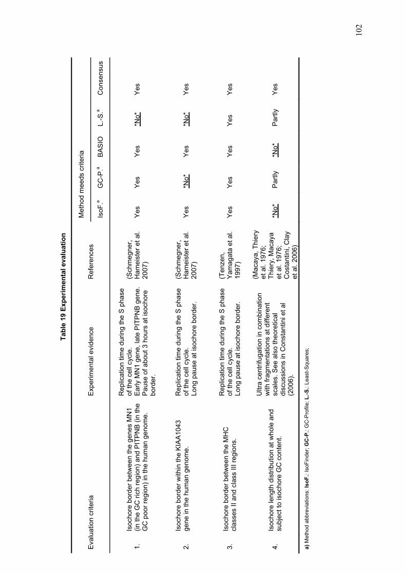
102
Tabl
e 19
Exp
erim
enta
l eva
luat
ion
Eva
luat
ion
crite
ria
Exp
erim
enta
l evi
denc
e R
efer
ence
s M
etho
d m
eeds
crit
eria
IsoF
.a G
C-P
.a B
AS
IO
L.-S
.a C
onse
nsus
1.
Isoc
hore
bor
der b
etw
een
the
gene
s M
N1
(in th
e G
C ri
ch re
gion
) and
PIT
PN
B (i
n th
e G
C p
oor r
egio
n) in
the
hum
an g
enom
e.
Rep
licat
ion
time
durin
g th
e S
pha
se
of th
e ce
ll cy
cle.
E
arly
MN
1 ge
ne, l
ate
PIT
PN
B g
ene.
P
ause
of a
bout
3 h
ours
at i
soch
ore
bord
er.
(Sch
meg
ner,
Ham
eist
er e
t al.
2007
) Y
es
Yes
Y
es
*No*
Ye
s
2.
Isoc
hore
bor
der w
ithin
the
KIA
A10
43
gene
in th
e hu
man
gen
ome.
Rep
licat
ion
time
durin
g th
e S
pha
se
of th
e ce
ll cy
cle.
Lo
ng p
ause
at i
soch
ore
bord
er.
(Sch
meg
ner,
Ham
eist
er e
t al.
2007
) Y
es
*No*
Y
es
*No*
Ye
s
3.
Isoc
hore
bor
der b
etw
een
the
MH
C
clas
ses
II an
d cl
ass
III re
gion
s.
Rep
licat
ion
time
durin
g th
e S
pha
se
of th
e ce
ll cy
cle.
Lo
ng p
ause
at i
soch
ore
bord
er.
(Ten
zen,
Y
amag
ata
et a
l. 19
97)
Yes
Yes
Yes
Yes
Yes
4.
Isoc
hore
leng
th d
istri
butio
n at
who
le a
nd
subj
ect t
o is
ocho
re G
C c
onte
nt.
Ultr
a ce
ntrif
ugat
ion
in c
ombi
natio
n w
ith fr
agm
enta
tions
at d
iffer
ent
scal
es. S
ee a
lso
theo
retic
al
disc
ussi
ons
in C
onst
antin
i et a
l (2
006)
.
(Mac
aya,
Thi
ery
et a
l. 19
76;
Thie
ry, M
acay
a et
al.
1976
; C
osta
ntin
i, C
lay
et a
l. 20
06)
*No*
P
artly
*N
o*
Par
tly
Yes
a) M
etho
d ab
brev
iatio
ns: I
soF.
: Iso
Find
er; G
C-P
.: G
C-P
rofil
e; L
.-S.:
Leas
t-Squ
ares
;
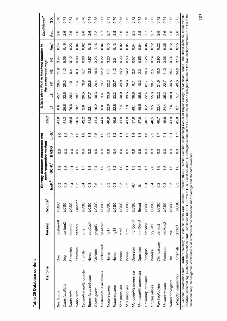
103
Tabl
e 20
Dat
abas
e co
nten
t
Gen
ome
Vers
ion
Sour
cea
Entr
opy
dist
ance
: con
sens
us a
nd
each
resp
ectiv
e m
etho
d %
GC
%
DN
A c
lass
ified
to is
ocho
re fa
mili
es in
th
e co
nsen
sus
map
C
onfid
ence
d
IsoF
.b G
C-P
.b B
ASI
O
L.-S
.b L1
L2
H
1 H
2 H
3 A
m.c
Avg
. SD
.
Bos
taur
us
Cow
bo
stau
4-0
H
GS
C
0.3
1.9
0.3
2.0
41.8
8.
6 45
.1
28.4
11
.9
3.44
0.
14
2.6
0.70
Can
is fa
mili
aris
D
og
canf
am2
U
CSC
0.
3 1.
3 0.
3 1.
2 41
.3
25.8
32
.5
20.3
11
.3
5.05
0.
16
2.6
0.71
Dan
io re
rio
Zebr
afis
h
danr
er4
U
CSC
0.
4 2.
1 0.
4 2.
3 36
.5
76.6
20
.4
1.9
0.4
0.12
0.
23
2.6
0.74
Dan
io re
rio
Zebr
afis
h
danr
er7
En
sem
bl
0.3
1.9
0.5
1.9
36.5
78
.1
20.1
1.
4 0.
3 0.
08
0.04
2.
6 0.
76
Dro
soph
ila m
elan
ogas
ter
Frui
t fly
dm
2
UC
SC
0.
4 1.
7 0.
4 1.
8 42
.2
2.6
20.5
70
.8
5.7
0.06
0.
02
2.6
0.76
Equ
us fe
rus
caba
llus
H
orse
eq
uCab
1
UC
SC
0.3
1.3
0.2
1.4
41.5
22
.1
37.7
22
.8
12.5
4.
57
0.16
2.
6 0.
71
Gal
lus
gallu
s
Chi
cken
ga
lgal
3
UC
SC
0.6
0.4
0.6
0.5
41.3
16
.2
40.3
26
.4
10.6
3.
23
1.16
2.
2 0.
58
Gas
tero
steu
s ac
ulea
tus
S
tickl
ebac
k
gasA
cu1
U
CS
C
0.3
1.9
0.3
1.9
44.6
0.
0 3.
4 73
.7
22.2
0.
22
0.04
2.
7 0.
77
Hom
o sa
pien
s
Hum
an
hg17
U
CS
C
0.3
0.3
0.6
0.3
40.9
22
.6
33.6
22
.2
11.1
3.
20
0.13
2.
7 0.
73
Hom
o sa
pien
s
Hum
an
hg18
U
CS
C
0.3
1.2
0.4
1.2
40.9
22
.8
33.2
22
.7
11.2
3.
01
0.13
2.
5 0.
70
Mus
mus
culu
s
Mou
se
mm
8
UC
SC
0.
3 1.
0 0.
6 1.
1 41
.8
7.4
40.0
34
.9
14.2
0.
33
0.02
2.
6 0.
68
Mus
mus
culu
s
Mou
se
mm
9
UC
SC
0.
3 1.
1 0.
5 1.
2 41
.8
7.9
39.5
34
.6
14.2
0.
50
0.01
2.
6 0.
72
Mon
odel
phis
dom
estic
a
Opo
ssum
m
onD
om4
U
CS
C
-0.1
1.
3 0.
8 1.
4 37
.8
49.1
36
.6
9.7
2.3
0.57
0.
54
2.5
0.72
Mon
odel
phis
dom
estic
a
Opo
ssum
m
onD
om5
B
road
-0
.1
1.3
0.8
1.4
37.8
49
.5
35.8
10
.2
2.3
0.55
0.
64
2.5
0.72
Orn
ithor
hy. a
natin
us
Plat
ypus
or
nAna
1
UC
SC
0.4
1.7
0.3
1.8
45.1
0.
2 22
.4
61.7
14
.3
1.25
0.
06
2.7
0.75
Ory
zias
latip
es
Med
eka
or
yLat
1
UC
SC
0.4
2.0
0.3
2.2
40.5
3.
5 55
.3
30.7
2.
5 0.
14
0.12
2.
7 0.
75
Pan
trog
lody
tes
C
him
panz
ee
pant
ro2
U
CSC
0.
2 1.
6 0.
3 1.
7 40
.7
22.4
32
.2
21.6
10
.5
2.90
0.
22
2.6
0.72
Mac
aca
mul
atta
M
acaq
ue
rheM
ac2
U
CSC
0.
3 1.
8 0.
3 2.
1 40
.6
24.4
35
.2
22.7
11
.0
3.06
0.
35
2.6
0.71
Rat
tus
norv
egic
us
Rat
rn
4
UC
SC
0.
3 1.
9 0.
3 2.
1 41
.9
7.6
38.0
34
.5
15.7
0.
74
0.12
2.
6 0.
72
Tetra
odon
nig
rovi
ridis
P
uffe
rfish
te
tNig
1 U
CS
C
0.3
1.6
0.3
1.7
45.8
0.
1 5.
7 49
.3
34.8
3.
16
0.15
2.
6 0.
75
a) G
enom
e do
wnl
oade
d fro
m:
UC
SC:
Uni
vers
ity o
f C
alifo
rnia
San
ta C
ruz
Gen
ome
Bro
wse
r; H
GSC
: H
uman
Gen
ome
Seq
uenc
ing
Cen
ter
at B
aylo
r C
olle
ge o
f M
edic
ine;
Bro
ad:
The
Bro
ad I
nstit
ute,
bro
ad.m
it.ed
u;
Ense
mbl
: ens
embl
.org
b) M
etho
d ab
brev
iatio
ns: I
soF.
: Iso
Find
er; G
C-P
.: G
C-P
rofil
e; L
.-S.:
Leas
t-Squ
ares
; c)
Am
bigu
ous
amou
nt o
f DN
A th
at c
ould
not
be
assi
gned
to o
ne o
f the
five
isoc
hore
fam
ilies
L1
to H
3 in
the
cons
ensu
s m
ap. d
) Ass
ignm
ent c
onfid
ence
of a
ll st
retc
hes
in th
e co
nsen
sus
map
: ave
rage
and
sta
ndar
d de
viat
ion
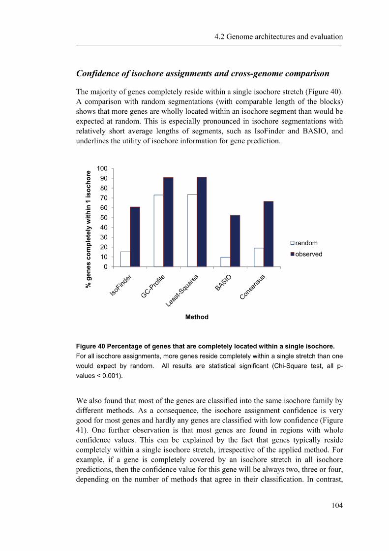
4.2 Genome architectures and evaluation
104
Confidence of isochore assignments and cross-genome comparison
The majority of genes completely reside within a single isochore stretch (Figure 40). A comparison with random segmentations (with comparable length of the blocks) shows that more genes are wholly located within an isochore segment than would be expected at random. This is especially pronounced in isochore segmentations with relatively short average lengths of segments, such as IsoFinder and BASIO, and underlines the utility of isochore information for gene prediction.
Figure 40 Percentage of genes that are completely located within a single isochore. For all isochore assignments, more genes reside completely within a single stretch than one would expect by random. All results are statistical significant (Chi-Square test, all p-values < 0.001).
We also found that most of the genes are classified into the same isochore family by different methods. As a consequence, the isochore assignment confidence is very good for most genes and hardly any genes are classified with low confidence (Figure 41). One further observation is that most genes are found in regions with whole confidence values. This can be explained by the fact that genes typically reside completely within a single isochore stretch, irrespective of the applied method. For example, if a gene is completely covered by an isochore stretch in all isochore predictions, then the confidence value for this gene will be always two, three or four, depending on the number of methods that agree in their classification. In contrast,
0102030405060708090
100
% g
enes
com
plet
ely
with
in 1
isoc
hore
Method
random
observed
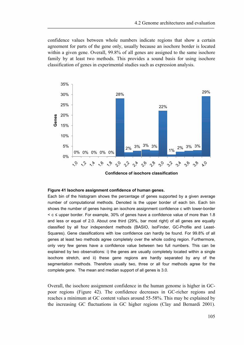
4.2 Genome architectures and evaluation
105
confidence values between whole numbers indicate regions that show a certain agreement for parts of the gene only, usually because an isochore border is located within a given gene. Overall, 99.8% of all genes are assigned to the same isochore family by at least two methods. This provides a sound basis for using isochore classification of genes in experimental studies such as expression analysis.
Figure 41 Isochore assignment confidence of human genes. Each bin of the histogram shows the percentage of genes supported by a given average number of computational methods. Denoted is the upper border of each bin. Each bin shows the number of genes having an isochore assignment confidence c with lower-border < c ≤ upper border. For example, 30% of genes have a confidence value of more than 1.8 and less or equal of 2.0. About one third (29%, bar most right) of all genes are equally classified by all four independent methods (BASIO, IsoFinder, GC-Profile and Least-Squares). Gene classifications with low confidence can hardly be found. For 99.8% of all genes at least two methods agree completely over the whole coding region. Furthermore, only very few genes have a confidence value between two full numbers. This can be explained by two observations: i) the genes are usually completely located within a single isochore stretch, and ii) these gene regions are hardly separated by any of the segmentation methods. Therefore usually two, three or all four methods agree for the complete gene. The mean and median support of all genes is 3.0.
Overall, the isochore assignment confidence in the human genome is higher in GC-poor regions (Figure 42). The confidence decreases in GC-richer regions and reaches a minimum at GC content values around 55-58%. This may be explained by the increasing GC fluctuations in GC higher regions (Clay and Bernardi 2001).
0% 0% 0% 0% 0%
28%
2% 3% 3% 3%
22%
1% 2% 3% 3%
29%
0%
5%
10%
15%
20%
25%
30%
35%
Gen
es
Confidence of isochore classification
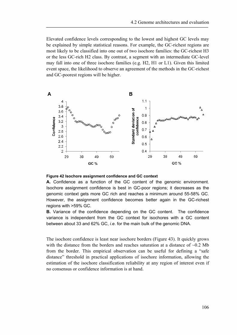
4.2 Genome architectures and evaluation
106
Elevated confidence levels corresponding to the lowest and highest GC levels may be explained by simple statistical reasons. For example, the GC-richest regions are most likely to be classified into one out of two isochore families: the GC-richest H3 or the less GC-rich H2 class. By contrast, a segment with an intermediate GC-level may fall into one of three isochore families (e.g. H2, H1 or L1). Given this limited event space, the likelihood to observe an agreement of the methods in the GC-richest and GC-poorest regions will be higher.
Figure 42 Isochore assignment confidence and GC context A. Confidence as a function of the GC content of the genomic environment. Isochore assignment confidence is best in GC-poor regions; it decreases as the genomic context gets more GC rich and reaches a minimum around 55-58% GC. However, the assignment confidence becomes better again in the GC-richest regions with >59% GC. B. Variance of the confidence depending on the GC content. The confidence variance is independent from the GC context for isochores with a GC content between about 33 and 62% GC, i.e. for the main bulk of the genomic DNA.
The isochore confidence is least near isochore borders (Figure 43). It quickly grows with the distance from the borders and reaches saturation at a distance of ~0.2 Mb from the border. This empirical observation can be useful for defining a “safe distance” threshold in practical applications of isochore information, allowing the estimation of the isochore classification reliability at any region of interest even if no consensus or confidence information is at hand.
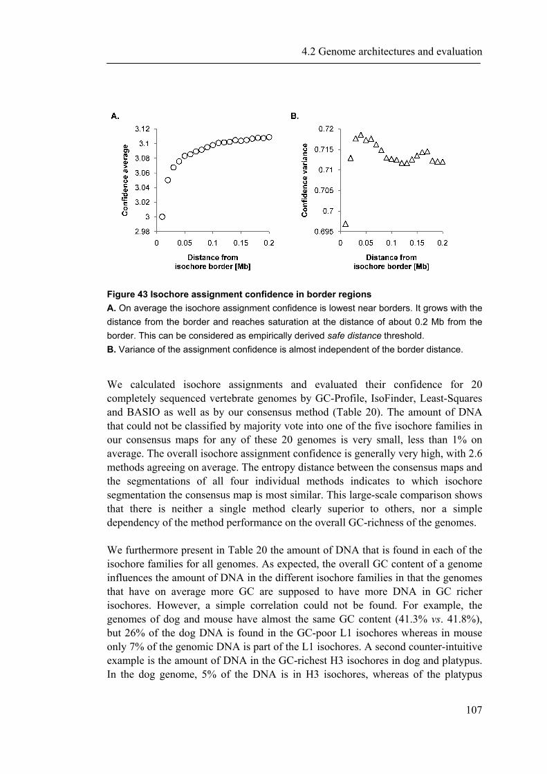
4.2 Genome architectures and evaluation
107
Figure 43 Isochore assignment confidence in border regions A. On average the isochore assignment confidence is lowest near borders. It grows with the distance from the border and reaches saturation at the distance of about 0.2 Mb from the border. This can be considered as empirically derived safe distance threshold. B. Variance of the assignment confidence is almost independent of the border distance.
We calculated isochore assignments and evaluated their confidence for 20 completely sequenced vertebrate genomes by GC-Profile, IsoFinder, Least-Squares and BASIO as well as by our consensus method (Table 20). The amount of DNA that could not be classified by majority vote into one of the five isochore families in our consensus maps for any of these 20 genomes is very small, less than 1% on average. The overall isochore assignment confidence is generally very high, with 2.6 methods agreeing on average. The entropy distance between the consensus maps and the segmentations of all four individual methods indicates to which isochore segmentation the consensus map is most similar. This large-scale comparison shows that there is neither a single method clearly superior to others, nor a simple dependency of the method performance on the overall GC-richness of the genomes. We furthermore present in Table 20 the amount of DNA that is found in each of the isochore families for all genomes. As expected, the overall GC content of a genome influences the amount of DNA in the different isochore families in that the genomes that have on average more GC are supposed to have more DNA in GC richer isochores. However, a simple correlation could not be found. For example, the genomes of dog and mouse have almost the same GC content (41.3% vs. 41.8%), but 26% of the dog DNA is found in the GC-poor L1 isochores whereas in mouse only 7% of the genomic DNA is part of the L1 isochores. A second counter-intuitive example is the amount of DNA in the GC-richest H3 isochores in dog and platypus. In the dog genome, 5% of the DNA is in H3 isochores, whereas of the platypus
4.2 Genome architectures and evaluation
108
genome merely 1% is in the H3 isochores. The opposite would have been expected as the platypus genome has a high overall GC content (46%) in comparison to a much lower GC content (41%) of the dog genome.
Availability and database content
We created an online database IsoBase where all data described in this study are freely accessible. Our website enables the user to evaluate statistical distributions of isochore properties, and compare isochore assignments within and between organisms and methods. Multiple qualitative and quantitative properties of isochore maps can be interactively explored. For each consensus isochore map confidence values of each segment are displayed. Table 20 shows an overview of genomes included in our database and their isochore properties. For convenient usage, we provide two search interfaces at our IsoBase website. The first search feature allows to look-up the genomic positions and the isochore families of genes by free text searches and by multiple identifier types. Currently genes can be looked-up by RefSeq identifiers, UniProt/SwissProt accessions, Ensembl IDs, gene and protein names, as well as by their descriptions, and SwissProt keywords. The second search option allows retrieval of available isochore information for a list of genomic positions in one step. All isochore assignments and the corresponding confidence information can be visualized online and downloaded as tab-delimited data files. In addition, we provide UCSC custom annotation tracks of the consensus isochore assignments for all genomes. All UCSC tracks can be downloaded from our web site. Furthermore, the isochore tracks are integrated into the UCSC view automatically by using the links to the UCSC genome browser at our web site.
4.2 Genome architectures and evaluation
109
4.2.4 Discussion
We have demonstrated that available isochore assignment approaches produce significantly different segmentations in terms of the location of isochore borders and the GC differences between neighboring stretches. At the same time, the total amount of genomic DNA classified into the same isochore family is very large, with all methods being in perfect agreement for more than two thirds of the human genome. The consensus isochore assignment method based on the majority vote at each genomic position has four distinct advantages. First, it provides a more balanced isochore assignment that is more robust against under -and over fragmentation. Secondly, it appears to produce more biologically relevant results as judged by a better correlation between the resulting segmentation and gene density. Thirdly, evaluation based on experimentally derived isochore data shows that our consensus approach is in a better accordance with all criteria than individual methods. Finally, our procedure allows estimating the reliability of the isochore assignments. We suggest that the consensus method has the potential to be further improved in the future by adding more complementary datasets. We have demonstrated that the majority of genes reside within a single isochore stretch and can be classified with high confidence. The isochore assignments become very reliable at the distance of about 0.2 Mb from the isochore borders. This empirical observation allows to estimate the assignment confidence even in the absence of any further knowledge. In conclusion, we recommend using consensus assignments for best confidence and best accordance to biological models that were found to be associated with isochores. We further demonstrated that the consensus approach is more robust than relying on a single method alone. At our website IsoBase, we provide isochore consensus assignments for all completely sequenced vertebrate genomes along with confidence information for visual exploration, search and downloading. We will add isochore consensus maps for new genomes as they become available. We hope that this resource will stimulate further analysis and exploration of the large-scale variation of genome properties.
Chapter 5 Conclusions and future work
The progress towards -and beyond- personalized medicine, epigenetic understanding and systemic analysis of multifactorial diseases results in avalanches of data. For example, a single high-throughput proteomic mass-spec experiment generates billion of data points already. Analyses of metabolite time courses, non-coding RNA, and genomic variants like single nucleotide polymorphism exponentiate our space of information. It is without any doubt, that in-depth manual analysis of the increasing data basis is beyond feasibility. Therefore, fundamental steps, in a typical analysis, are to integrate the knowledge spheres of interest and to deduce new information by contrasting data domains. A classical example would be to compare the change of expression and function over a time course experiment. Actually, comparison of large biological datasets has become a prime task in bioinformatics. In this context and in general, mapping and data integration are essential steps in almost any computational analysis by now. In this work we developed a multitude of new methods for comparative proteomics that intelligibly promote this field of research (Schmidt and Frishman 2006; Schmidt and Frishman 2006; Smialowski, Schmidt et al. 2006; Hager 2007; Schmidt, Hombach et al. 2007; Antonov, Schmidt et al. 2008; Irmler, Hartl et al. 2008; Ishihama, Schmidt et al. 2008; Schmidt and Frishman 2008). We further applied the new technologies to multiple biological questions and thus inferred quite a few new insights (Smialowski, Schmidt et al. 2006; Schmidt, Hombach et al. 2007; Irmler, Hartl et al. 2008; Ishihama, Schmidt et al. 2008; Schmidt and Frishman 2008). Besides we contributed to numerous databases and tools yielding to advances even beyond the scope of work (Riley, Schmidt et al. 2005; Riley, Schmidt et al. 2007; Ruepp, Brauner et al. 2007; Schmidt, Hombach et al. 2007; Irmler, Hartl et al. 2008) . Comparative proteomic analyses can be broken down into a number of subtasks. In the following a short condensation of the main points is outlined. For details about all methodical details, data sources, and full results the reference to the respective chapter of this work is given.
Summary
111
Summary
The new software described in chapter 2, PROMPT (Schmidt and Frishman 2006), is a versatile, platform-independent, easily expandable, stand-alone application. PROMPT proved to be a practical workhorse in analyzing and mining protein sequences and associated annotation. Its availability of a Java Application Programming Interface and scripting capabilities on one hand, and the intuitive Graphical User Interface with context-sensitive help system on the other, make it equally accessible to professional bioinformaticians as well as to biologically-oriented users. In chapter 2.2, we further demonstrated that the PROMPT tool can provide an additional independent layer of evidence to results obtained by existing functional analysis tools. The integration of structural and physical features into data analysis tools provides complementary means for functional interpretation (Irmler, Hartl et al. 2008). The design of PROMPT allows the implementation of additional transcript and protein data in the future. It is freely available for academic users at our web page. More than 6,000 downloads and already 9 citations in high-ranking journals motivated us to constantly improve the functionality of PROMPT. In chapter 3, additionally developed methods, data resources and applications are presented. The first section of chapter 3, showed an outline of co-developed databases (Riley, Schmidt et al. 2005; Riley, Schmidt et al. 2007; Ruepp, Brauner et al. 2007) and powerful data retrieval systems (Schmidt and Frishman 2006; Riley, Schmidt et al. 2007; Ruepp, Brauner et al. 2007). In the second section of chapter 3, we illustrated how the developed comparative approach in conjunction with our data resources can be used for predicting protein properties. As result, we proposed a machine-learning approach to sequence-based prediction of protein crystallizability and demonstrated that small sequence-based features impact the possibility to yield a protein crystal (Smialowski, Schmidt et al. 2006). In the last section of chapter 3, we introduced a new procedure to reveal “complex functions” of gene and protein sets. A so called “complex function” is constructed as Boolean combination of available annotation terms. We described a new web-tool named ProfCom that is able to infer new previously hidden functional roles of gene/protein sets. We showed that we could not only confirm previous theories about up-regulated genes of two human cancer types, but add additional hypotheses that may inspire further experiments (Antonov, Schmidt et al. 2008). Finally, in chapter 4, we present the first large-scale abundance measurement and profiling for more than 1000 E. coli proteins. This represents the most complete study of protein abundance in a bacterial cell so far. We showed significant associations between the abundance of a protein and its properties and functions in
Summary
112
the cell. In this way, we provided both data and novel insights into the role of protein concentration in this model organism (Ishihama, Schmidt et al. 2008). Additionally, in the second part of chapter 4, we further questioned the impact of underlying genome architectures. The genomes of higher organisms show non-random patterns of fairly homogenous GC content that are commonly referred as isochores. Multiple experimental evidences showed the impact of isochores for gene expression, regulation, and replication timing (see chapters 1 and 4 for details). As consequence, we investigated the genome-architecture at large-scale. Here, we presented a new consensus isochore assignment method based on a majority voting and evaluated it against the currently available body of isochore knowledge. The isochores derived by the consensus approach correlate better with the distribution of gene density and experimental evidence than individual methods. We provide a measure of the isochore assignment confidence based on the number of methods that agree for a given base pair and demonstrate how the confidence depends on GC content and the distance to isochore border regions. Finally, we provide IsoBase - a comprehensive on-line database of isochore maps for all completely sequenced vertebrate genomes - that enables the user to evaluate statistical distributions of isochore properties and compare isochore assignments between organisms and methods (Schmidt and Frishman 2008). We showed that the developed tools and methods contribute to the field of comparative proteomics in many ways. The field of applications in this thesis range from proteomic investigations- up to genomic background analyzes. Beyond, this work extended the field of functional profiling and provided new biological insights and hypotheses in E.coli (chapter 4.1), mouse (chapter 2.2) and human (chapter 3.3).
113
List of Tables
Table 1 Overview of possible data inputs. ................................................................ 21 Table 2 Summary of PROMPT’s generic comparison methods. .............................. 24 Table 3 PROMPT analysis results ............................................................................ 44 Table 4 Amino acid grouping ................................................................................... 55 Table 5 Confusion Matrix for Naive Bayes Meta-classifier ..................................... 56 Table 6 Data files used by ProfCom to automatically retrieve annotations. ............. 58 Table 7 Types of gene identifiers recognized by ProfCom and data sources used for ID mapping. ............................................................................................................... 59 Table 8 Performance comparison ProfCom vs. GENECODIS ................................. 62 Table 9 Feature comparison ProfCom vs. GENECODIS ......................................... 63 Table 10 E.coli cytosol. ............................................................................................. 69 Table 11 Comparison of predicted peptides and observed peptides. ........................ 73 Table 12 The most abundant functional groups in the E. coli cytosol ...................... 79 Table 13 Most abundant protein folds in the E. coli cytosol .................................... 82 Table 14 Comparison of features associated with protein aggregation between high abundant proteins and the remaining detected proteins. ........................................... 83 Table 15 Entropy distance ......................................................................................... 95 Table 16 The amount of genomic DNA in which methods agree (%) ...................... 96 Table 17 Agreement on gene classification (%) ....................................................... 96 Table 18 Isochores and gene density ........................................................................ 99 Table 19 Experimental evaluation .......................................................................... 102 Table 20 Database content ...................................................................................... 103

114
List of Figures
Figure 1 General Workflow of PROMPT ................................................................. 17 Figure 2 PROMPT Software architecture. ................................................................ 18 Figure 3 Example PROMPT XML File. ................................................................... 20 Figure 4 Document Type Definition (DTD) of PROMPT's generic XML format ... 21 Figure 5 Data input and mapping workflow ............................................................. 22 Figure 6 Screenshot of the PROMPT web page. ...................................................... 26 Figure 7 Graphical User Interface (GUI). ................................................................. 28 Figure 8 Screenshots of a typical statistical test dialog. ............................................ 29 Figure 9 Built-in help system. ................................................................................... 30 Figure 10 Example of an interactive browsable figure. ............................................ 31 Figure 11 Example of a categorical comparison analysis. ........................................ 32 Figure 12 Results of a correlation analysis. .............................................................. 33 Figure 13 Comparison of two numeric distributions by PROMPT. ......................... 34 Figure 14 Examples of built-in interactive plots. ...................................................... 35 Figure 15 Binning wizard for setting up interval borders. ........................................ 36 Figure 16 Screenshots of PROMPT’s visualisations of the sequence based symbol analysis methods. ...................................................................................................... 38 Figure 17 Illustration of the functional and structural content of the PEDANT database. .................................................................................................................... 46 Figure 18 FunCat distribution ................................................................................... 46 Figure 19 Web Service communication schema ....................................................... 47 Figure 20 PROMPT-PEDANT integration ............................................................... 49 Figure 21 Screenshot of a complex entry. ................................................................. 50 Figure 22 CORUM Search and FunCat browser. ..................................................... 51 Figure 23 Screenshot of the ProfCom web page ....................................................... 64 Figure 24 Reproducibility of emPAI values for replicate biological samples of E. coli cytosol. ............................................................................................................... 74 Figure 25 Correlation between observed emPAI values and independently measured protein copy numbers per cell. .................................................................................. 75 Figure 26 Observed concentration and protein detection frequencies. ..................... 76 Figure 27 Abundance distribution of all identified proteins. .................................... 78 Figure 28 Abundance functional profile. .................................................................. 80 Figure 29 Abundance distribution of proteins classified according to the EC Enzyme classification scheme. ................................................................................................ 81 Figure 30 Abundance and essentiality. ..................................................................... 84 Figure 31 Abundance vs. Protein length ................................................................... 85 Figure 32 Abundance versus codon adaptation index (CAI). ................................... 86
115
Figure 33 Karlin’s predicted gene expression and measured protein abundance. .... 86 Figure 34 Variance of abundance within known operons. ........................................ 87 Figure 35 Comparison of isochore assignments in the human genome made by different methods. ..................................................................................................... 93 Figure 36 GC differences between neighboring isochores. ...................................... 94 Figure 37 Distances between the isochore borders produced by different methods . 95 Figure 38 Graphical representation of the isochore assignments for the first 100 Mb of the human chromosome 1. .................................................................................... 98 Figure 39 Correlation between isochore classification and gene density. .............. 100 Figure 40 Percentage of genes that are completely located within a single isochore. ................................................................................................................................. 104 Figure 41 Isochore assignment confidence of human genes. .................................. 105 Figure 42 Isochore assignment confidence and GC context ................................... 106 Figure 43 Isochore assignment confidence in border regions ................................. 107
116
Bibliography
Al‐Shahrour, F., R. az‐Uriarte and J. Dopazo (2004). "FatiGO: a web tool for finding
significant associations of Gene Ontology terms with groups of genes." Bioinformatics. 20(4): 578‐580.
Al‐Shahrour, F., P. Minguez, J. Tarraga, I. Medina, E. Alloza, D. Montaner and J. Dopazo (2007). "FatiGO +: a functional profiling tool for genomic data. Integration of functional annotation, regulatory motifs and interaction data with microarray experiments." Nucleic Acids Res. 35(Web Server issue): W91‐W96.
Al‐Shahrour, F., P. Minguez, J. Tarraga, D. Montaner, E. Alloza, J. M. Vaquerizas, L. Conde, C. Blaschke, J. Vera and J. Dopazo (2006). "BABELOMICS: a systems biology perspective in the functional annotation of genome‐scale experiments." Nucleic Acids Res. 34(Web Server issue): W472‐W476.
Al‐Shahrour, F., P. Minguez, J. M. Vaquerizas, L. Conde and J. Dopazo (2005). "BABELOMICS: a suite of web tools for functional annotation and analysis of groups of genes in high‐throughput experiments." Nucleic Acids Res. 33(Web Server issue): W460‐W464.
Altschul, S. F., W. Gish, W. Miller, E. W. Myers and D. J. Lipman (1990). "Basic local alignment search tool." J Mol Biol 215(3): 403‐10.
Altschul, S. F., T. L. Madden, A. A. Schaffer, J. Zhang, Z. Zhang, W. Miller and D. J. Lipman (1997). "Gapped BLAST and PSI‐BLAST: a new generation of protein database search programs." Nucleic Acids Res 25(17): 3389‐402.
Andreeva, A., D. Howorth, S. E. Brenner, T. J. Hubbard, C. Chothia and A. G. Murzin (2004). "SCOP database in 2004: refinements integrate structure and sequence family data." Nucleic Acids Res 32(Database issue): D226‐9.
Antonov, A. V. and H. W. Mewes (2006). "BIOREL: the benchmark resource to estimate the relevance of the gene networks." FEBS Lett. 580(3): 844‐848.
Antonov, A. V. and H. W. Mewes (2006). "Complex functionality of gene groups identified from high‐throughput data." J.Mol.Biol. 363(1): 289‐296.
Antonov, A. V., T. Schmidt, Y. Wang and H. W. Mewes (2008). "ProfCom: profiling the complex functionality of gene groups identified from high‐thoughput data." Nucleic Acids Res * joint first authors: in press.
Antonov, A. V., I. V. Tetko and H. W. Mewes (2006). "A systematic approach to infer biological relevance and biases of gene network structures." Nucleic Acids Res. 34(1): e6.
Apweiler, R., T. K. Attwood, A. Bairoch, A. Bateman, E. Birney, M. Biswas, P. Bucher, L. Cerutti, F. Corpet, M. D. Croning, R. Durbin, L. Falquet, W. Fleischmann, J. Gouzy, H. Hermjakob, N. Hulo, I. Jonassen, D. Kahn, A. Kanapin, Y. Karavidopoulou, R. Lopez, B. Marx, N. J. Mulder, T. M. Oinn, M. Pagni, F. Servant, C. J. Sigrist and E. M. Zdobnov (2001). "The InterPro database, an integrated documentation resource for protein families, domains and functional sites." Nucleic Acids Res. 29(1): 37‐40.
Ashburner, M., C. A. Ball, J. A. Blake, D. Botstein, H. Butler, J. M. Cherry, A. P. Davis, K. Dolinski, S. S. Dwight, J. T. Eppig, M. A. Harris, D. P. Hill, L. Issel‐Tarver, A. Kasarskis, S. Lewis, J. C. Matese, J. E. Richardson, M. Ringwald, G. M. Rubin and G. Sherlock (2000). "Gene ontology: tool for the unification of biology. The Gene Ontology
117
Consortium." Nat Genet 25(1): 25‐9. Bairoch, A., R. Apweiler, C. H. Wu, W. C. Barker, B. Boeckmann, S. Ferro, E. Gasteiger, H.
Huang, R. Lopez, M. Magrane, M. J. Martin, D. A. Natale, C. O'Donovan, N. Redaschi and L. S. Yeh (2005). "The Universal Protein Resource (UniProt)." Nucleic Acids Res 33(Database issue): D154‐9.
Bantscheff, M., M. Schirle, G. Sweetman, J. Rick and B. Kuster (2007). "Quantitative mass spectrometry in proteomics: a critical review." Anal Bioanal Chem 389(4): 1017‐31.
Barr, J. R., V. L. Maggio, D. G. Patterson, Jr., G. R. Cooper, L. O. Henderson, W. E. Turner, S. J. Smith, W. H. Hannon, L. L. Needham and E. J. Sampson (1996). "Isotope dilution‐‐mass spectrometric quantification of specific proteins: model application with apolipoprotein A‐I." Clin Chem 42(10): 1676‐82.
Benson, D. A., I. Karsch‐Mizrachi, D. J. Lipman, J. Ostell and D. L. Wheeler (2005). "GenBank." Nucleic Acids Res 33(Database issue): D34‐8.
Berman, H. M., J. Westbrook, Z. Feng, G. Gilliland, T. N. Bhat, H. Weissig, I. N. Shindyalov and P. E. Bourne (2000). "The Protein Data Bank." Nucleic Acids Res 28(1): 235‐42.
Bernardi, G. (1989). "The isochore organization of the human genome." Annu Rev Genet 23: 637‐61.
Bernardi, G. (2007). "The neoselectionist theory of genome evolution." Proc Natl Acad Sci U S A 104(20): 8385‐90.
Berriz, G. F., O. D. King, B. Bryant, C. Sander and F. P. Roth (2003). "Characterizing gene sets with FuncAssociate." Bioinformatics. 19(18): 2502‐2504.
Bertone, P., Y. Kluger, N. Lan, D. Zheng, D. Christendat, A. Yee, A. M. Edwards, C. H. Arrowsmith, G. T. Montelione and M. Gerstein (2001). "SPINE: an integrated tracking database and data mining approach for identifying feasible targets in high‐throughput structural proteomics." Nucleic Acids Res 29(13): 2884‐98.
Beyer, A., J. Hollunder, H. P. Nasheuer and T. Wilhelm (2004). "Post‐transcriptional expression regulation in the yeast Saccharomyces cerevisiae on a genomic scale." Mol Cell Proteomics 3(11): 1083‐92.
Birney, E., D. Andrews, M. Caccamo, Y. Chen, L. Clarke, G. Coates, T. Cox, F. Cunningham, V. Curwen, T. Cutts, T. Down, R. Durbin, X. M. Fernandez‐Suarez, P. Flicek, S. Graf, M. Hammond, J. Herrero, K. Howe, V. Iyer, K. Jekosch, A. Kahari, A. Kasprzyk, D. Keefe, F. Kokocinski, E. Kulesha, D. London, I. Longden, C. Melsopp, P. Meidl, B. Overduin, A. Parker, G. Proctor, A. Prlic, M. Rae, D. Rios, S. Redmond, M. Schuster, I. Sealy, S. Searle, J. Severin, G. Slater, D. Smedley, J. Smith, A. Stabenau, J. Stalker, S. Trevanion, A. Ureta‐Vidal, J. Vogel, S. White, C. Woodwark and T. J. Hubbard (2006). "Ensembl 2006." Nucleic Acids Res. 34(Database issue): D556‐D561.
Blattner, F. R., G. Plunkett, 3rd, C. A. Bloch, N. T. Perna, V. Burland, M. Riley, J. Collado‐Vides, J. D. Glasner, C. K. Rode, G. F. Mayhew, J. Gregor, N. W. Davis, H. A. Kirkpatrick, M. A. Goeden, D. J. Rose, B. Mau and Y. Shao (1997). "The complete genome sequence of Escherichia coli K‐12." Science 277(5331): 1453‐74.
Boeckmann, B., A. Bairoch, R. Apweiler, M. C. Blatter, A. Estreicher, E. Gasteiger, M. J. Martin, K. Michoud, C. O'Donovan, I. Phan, S. Pilbout and M. Schneider (2003). "The SWISS‐PROT protein knowledgebase and its supplement TrEMBL in 2003." Nucleic Acids Res 31(1): 365‐70.
Cai, C. Z., L. Y. Han, Z. L. Ji, X. Chen and Y. Z. Chen (2003). "SVM‐Prot: Web‐based support vector machine software for functional classification of a protein from its primary sequence." Nucleic Acids Res 31(13): 3692‐7.
Calamai, M., N. Taddei, M. Stefani, G. Ramponi and F. Chiti (2003). "Relative influence of hydrophobicity and net charge in the aggregation of two homologous proteins."
118
Biochemistry 42(51): 15078‐83. Carmona‐Saez, P., M. Chagoyen, F. Tirado, J. M. Carazo and A. Pascual‐Montano (2007).
"GENECODIS: a web‐based tool for finding significant concurrent annotations in gene lists." Genome Biol. 8(1): R3.
Carmona‐Saez, P., M. Chagoyen, F. Tirado, J. M. Carazo and A. Pascual‐Montano (2007). "GENECODIS: a web‐based tool for finding significant concurrent annotations in gene lists." Genome Biol 8(1): R3.
Castillo‐Davis, C. I. and D. L. Hartl (2003). "GeneMerge‐‐post‐genomic analysis, data mining, and hypothesis testing." Bioinformatics 19(7): 891‐2.
Chen, L., R. Oughtred, H. M. Berman and J. Westbrook (2004). "TargetDB: a target registration database for structural genomics projects." Bioinformatics 20(16): 2860‐2.
Chiti, F., M. Stefani, N. Taddei, G. Ramponi and C. M. Dobson (2003). "Rationalization of the effects of mutations on peptide and protein aggregation rates." Nature 424(6950): 805‐8.
Christendat, D., A. Yee, A. Dharamsi, Y. Kluger, M. Gerstein, C. H. Arrowsmith and A. M. Edwards (2000). "Structural proteomics: prospects for high throughput sample preparation." Prog Biophys Mol Biol 73(5): 339‐45.
Clay, O. and G. Bernardi (2001). "Compositional heterogeneity within and among isochores in mammalian genomes. II. Some general comments." Gene 276(1‐2): 25‐31.
Clay, O., S. Caccio, S. Zoubak, D. Mouchiroud and G. Bernardi (1996). "Human coding and noncoding DNA: compositional correlations." Mol Phylogenet Evol 5(1): 2‐12.
Cochrane, G., P. Aldebert, N. Althorpe, M. Andersson, W. Baker, A. Baldwin, K. Bates, S. Bhattacharyya, P. Browne, A. van den Broek, M. Castro, K. Duggan, R. Eberhardt, N. Faruque, J. Gamble, C. Kanz, T. Kulikova, C. Lee, R. Leinonen, Q. Lin, V. Lombard, R. Lopez, M. McHale, H. McWilliam, G. Mukherjee, F. Nardone, M. P. Pastor, S. Sobhany, P. Stoehr, K. Tzouvara, R. Vaughan, D. Wu, W. Zhu and R. Apweiler (2006). "EMBL Nucleotide Sequence Database: developments in 2005." Nucleic Acids Res 34(Database issue): D10‐5.
Coghlan, A. and K. H. Wolfe (2000). "Relationship of codon bias to mRNA concentration and protein length in Saccharomyces cerevisiae." Yeast 16(12): 1131‐45.
Corbin, R. W., O. Paliy, F. Yang, J. Shabanowitz, M. Platt, C. E. Lyons, Jr., K. Root, J. McAuliffe, M. I. Jordan, S. Kustu, E. Soupene and D. F. Hunt (2003). "Toward a protein profile of Escherichia coli: comparison to its transcription profile." Proc Natl Acad Sci U S A 100(16): 9232‐7.
Costantini, M., O. Clay, F. Auletta and G. Bernardi (2006). "An isochore map of human chromosomes." Genome Res. 16(4): 536‐541.
Costantini, M., O. Clay, C. Federico, S. Saccone, F. Auletta and G. Bernardi (2006). "Human chromosomal bands: nested structure, high‐definition map and molecular basis." Chromosoma.
Cox, B., T. Kislinger and A. Emili (2005). "Integrating gene and protein expression data: pattern analysis and profile mining." Methods 35(3): 303‐14.
Cox, B., T. Kislinger, D. A. Wigle, A. Kannan, K. Brown, T. Okubo, B. Hogan, I. Jurisica, B. Frey, J. Rossant and A. Emili (2007). "Integrated proteomic and transcriptomic profiling of mouse lung development and Nmyc target genes." Mol Syst Biol 3: 109.
Cox, J. and M. Mann (2007). "Is proteomics the new genomics?" Cell 130(3): 395‐8. D'Onofrio, G., D. Mouchiroud, B. Aissani, C. Gautier and G. Bernardi (1991). "Correlations
between the compositional properties of human genes, codon usage, and amino acid composition of proteins." J Mol Evol 32(6): 504‐10.
119
Daniela Hartl, M. I., Irmgard Römer, Michael T. Mader, Lei Mao, Claus Zabel, Ferdinand von Meyenn, M. Hrabé de Angelis, Johannes Beckers, Joachim Klose "Analysis of mouse brain proteome and transcriptome rearrangement during early embryonic development." Proteomics accepted for publication.
Das, R. and M. Gerstein (2000). "The stability of thermophilic proteins: a study based on comprehensive genome comparison." Funct Integr Genomics 1(1): 76‐88.
Dempster, A. P., N. M. Laird and D. B. Rubin (1977). "Maximum likehood from incomplete data via the EM algorithm." J Roy Statist Soc 39(1): 1‐38.
Di Giulio, M. (2005). "A comparison of proteins from Pyrococcus furiosus and Pyrococcus abyssi: barophily in the physicochemical properties of amino acids and in the genetic code." Gene 346: 1‐6.
Draghici, S., P. Khatri, A. L. Tarca, K. Amin, A. Done, C. Voichita, C. Georgescu and R. Romero (2007). "A systems biology approach for pathway level analysis." Genome Res. 17(10): 1537‐1545.
Draghici, S., S. Sellamuthu and P. Khatri (2006). "Babel's tower revisited: a universal resource for cross‐referencing across annotation databases." Bioinformatics. 22(23): 2934‐2939.
DuBay, K. F., A. P. Pawar, F. Chiti, J. Zurdo, C. M. Dobson and M. Vendruscolo (2004). "Prediction of the absolute aggregation rates of amyloidogenic polypeptide chains." J Mol Biol 341(5): 1317‐26.
Duret, L., D. Mouchiroud and C. Gautier (1995). "Statistical analysis of vertebrate sequences reveals that long genes are scarce in GC‐rich isochores." J Mol Evol 40(3): 308‐17.
Eisenbarth, I., K. Beyer, W. Krone and G. Assum (2000). "Toward a survey of somatic mutation of the NF1 gene in benign neurofibromas of patients with neurofibromatosis type 1." Am J Hum Genet 66(2): 393‐401.
Engelman, D. M., T. A. Steitz and A. Goldman (1986). "Identifying nonpolar transbilayer helices in amino acid sequences of membrane proteins." Annu Rev Biophys Biophys Chem 15: 321‐53.
Eppig, J. T., C. J. Bult, J. A. Kadin, J. E. Richardson, J. A. Blake, A. Anagnostopoulos, R. M. Baldarelli, M. Baya, J. S. Beal, S. M. Bello, W. J. Boddy, D. W. Bradt, D. L. Burkart, N. E. Butler, J. Campbell, M. A. Cassell, L. E. Corbani, S. L. Cousins, D. J. Dahmen, H. Dene, A. D. Diehl, H. J. Drabkin, K. S. Frazer, P. Frost, L. H. Glass, C. W. Goldsmith, P. L. Grant, M. Lennon‐Pierce, J. Lewis, I. Lu, L. J. Maltais, M. McAndrews‐Hill, L. McClellan, D. B. Miers, L. A. Miller, L. Ni, J. E. Ormsby, D. Qi, T. B. Reddy, D. J. Reed, B. Richards‐Smith, D. R. Shaw, R. Sinclair, C. L. Smith, P. Szauter, M. B. Walker, D. O. Walton, L. L. Washburn, I. T. Witham and Y. Zhu (2005). "The Mouse Genome Database (MGD): from genes to mice‐‐a community resource for mouse biology." Nucleic Acids Res 33(Database issue): D471‐5.
Errington, J., R. A. Daniel and D. J. Scheffers (2003). "Cytokinesis in bacteria." Microbiol Mol Biol Rev 67(1): 52‐65.
Eyre‐Walker, A. and L. D. Hurst (2001). "The evolution of isochores." Nat Rev Genet 2(7): 549‐55.
Filipski, J., J. P. Thiery and G. Bernardi (1973). "An analysis of the bovine genome by Cs2SO4‐Ag density gradient centrifugation." J Mol Biol 80(1): 177‐97.
Finn, R. D., J. Tate, J. Mistry, P. C. Coggill, S. J. Sammut, H. R. Hotz, G. Ceric, K. Forslund, S. R. Eddy, E. L. Sonnhammer and A. Bateman (2008). "The Pfam protein families database." Nucleic Acids Res 36(Database issue): D281‐8.
Flicek, P., B. L. Aken, K. Beal, B. Ballester, M. Caccamo, Y. Chen, L. Clarke, G. Coates, F.
120
Cunningham, T. Cutts, T. Down, S. C. Dyer, T. Eyre, S. Fitzgerald, J. Fernandez‐Banet, S. Graf, S. Haider, M. Hammond, R. Holland, K. L. Howe, K. Howe, N. Johnson, A. Jenkinson, A. Kahari, D. Keefe, F. Kokocinski, E. Kulesha, D. Lawson, I. Longden, K. Megy, P. Meidl, B. Overduin, A. Parker, B. Pritchard, A. Prlic, S. Rice, D. Rios, M. Schuster, I. Sealy, G. Slater, D. Smedley, G. Spudich, S. Trevanion, A. J. Vilella, J. Vogel, S. White, M. Wood, E. Birney, T. Cox, V. Curwen, R. Durbin, X. M. Fernandez‐Suarez, J. Herrero, T. J. Hubbard, A. Kasprzyk, G. Proctor, J. Smith, A. Ureta‐Vidal and S. Searle (2008). "Ensembl 2008." Nucleic Acids Res 36(Database issue): D707‐14.
Forner, F., L. J. Foster, S. Campanaro, G. Valle and M. Mann (2006). "Quantitative proteomic comparison of rat mitochondria from muscle, heart, and liver." Mol Cell Proteomics 5(4): 608‐19.
Frishman, D. (2002). "Knowledge‐based selection of targets for structural genomics." Protein Eng 15(3): 169‐83.
Frishman, D. (2007). "Protein annotation at genomic scale: the current status." Chem Rev 107(8): 3448‐66.
Frishman, D., K. Albermann, J. Hani, K. Heumann, A. Metanomski, A. Zollner and H. W. Mewes (2001). "Functional and structural genomics using PEDANT." Bioinformatics 17(1): 44‐57.
Frishman, D. and P. Argos (1995). "Knowledge‐based protein secondary structure assignment." Proteins 23(4): 566‐79.
Frishman, D. and H. W. Mewes (1997). "Protein structural classes in five complete genomes." Nat Struct Biol 4(8): 626‐8.
Frishman, D., M. Mokrejs, D. Kosykh, G. Kastenmuller, G. Kolesov, I. Zubrzycki, C. Gruber, B. Geier, A. Kaps, K. Albermann, A. Volz, C. Wagner, M. Fellenberg, K. Heumann and H. W. Mewes (2003). "The PEDANT genome database." Nucleic Acids Res 31(1): 207‐11.
Fullerton, S. M., A. Bernardo Carvalho and A. G. Clark (2001). "Local rates of recombination are positively correlated with GC content in the human genome." Mol Biol Evol 18(6): 1139‐42.
Futcher, B., G. I. Latter, P. Monardo, C. S. McLaughlin and J. I. Garrels (1999). "A sampling of the yeast proteome." Mol Cell Biol 19(11): 7357‐68.
Gardiner, K. (1996). "Base composition and gene distribution: critical patterns in mammalian genome organization." Trends Genet 12(12): 519‐24.
Gardy, J. L., M. R. Laird, F. Chen, S. Rey, C. J. Walsh, M. Ester and F. S. Brinkman (2005). "PSORTb v.2.0: expanded prediction of bacterial protein subcellular localization and insights gained from comparative proteome analysis." Bioinformatics 21(5): 617‐23.
Gasteiger, E., E. Jung and A. Bairoch (2001). "SWISS‐PROT: connecting biomolecular knowledge via a protein database." Curr Issues Mol Biol 3(3): 47‐55.
Gentleman, R. C., V. J. Carey, D. M. Bates, B. Bolstad, M. Dettling, S. Dudoit, B. Ellis, L. Gautier, Y. Ge, J. Gentry, K. Hornik, T. Hothorn, W. Huber, S. Iacus, R. Irizarry, F. Leisch, C. Li, M. Maechler, A. J. Rossini, G. Sawitzki, C. Smith, G. Smyth, L. Tierney, J. Y. Yang and J. Zhang (2004). "Bioconductor: open software development for computational biology and bioinformatics." Genome Biol 5(10): R80.
Gerber, S. A., J. Rush, O. Stemman, M. W. Kirschner and S. P. Gygi (2003). "Absolute quantification of proteins and phosphoproteins from cell lysates by tandem MS." Proc Natl Acad Sci U S A 100(12): 6940‐5.
Gerdes, S. Y., M. D. Scholle, J. W. Campbell, G. Balazsi, E. Ravasz, M. D. Daugherty, A. L.
121
Somera, N. C. Kyrpides, I. Anderson, M. S. Gelfand, A. Bhattacharya, V. Kapatral, M. D'Souza, M. V. Baev, Y. Grechkin, F. Mseeh, M. Y. Fonstein, R. Overbeek, A. L. Barabasi, Z. N. Oltvai and A. L. Osterman (2003). "Experimental determination and system level analysis of essential genes in Escherichia coli MG1655." J Bacteriol 185(19): 5673‐84.
Gerstein, M. (1997). "A structural census of genomes: comparing bacterial, eukaryotic, and archaeal genomes in terms of protein structure." J Mol Biol 274(4): 562‐76.
Gerstein, M. and M. Levitt (1997). "A structural census of the current population of protein sequences." PNAS 94(22): 11911‐11916.
Ghaemmaghami, S., W.‐K. Huh, K. Bower, R. W. Howson, A. Belle, N. Dephoure, E. K. O'Shea and J. S. Weissman (2003). "Global analysis of protein expression in yeast." Nature 425(6959): 737‐741.
Gianese, G., F. Bossa and S. Pascarella (2002). "Comparative structural analysis of psychrophilic and meso‐ and thermophilic enzymes." Proteins 47(2): 236‐49.
Goffard, N. and G. Weiller (2007). "PathExpress: a web‐based tool to identify relevant pathways in gene expression data." Nucleic Acids Res. 35(Web Server issue): W176‐W181.
Goh, C. S., N. Lan, S. M. Douglas, B. Wu, N. Echols, A. Smith, D. Milburn, G. T. Montelione, H. Zhao and M. Gerstein (2004). "Mining the structural genomics pipeline: identification of protein properties that affect high‐throughput experimental analysis." J Mol Biol 336(1): 115‐30.
Greenbaum, D., R. Jansen and M. Gerstein (2002). "Analysis of mRNA expression and protein abundance data: an approach for the comparison of the enrichment of features in the cellular population of proteins and transcripts." Bioinformatics 18(4): 585‐96.
Gygi, S. P., B. Rist, S. A. Gerber, F. Turecek, M. H. Gelb and R. Aebersold (1999). "Quantitative analysis of complex protein mixtures using isotope‐coded affinity tags." Nat Biotechnol 17(10): 994‐9.
Gygi, S. P., Y. Rochon, B. R. Franza and R. Aebersold (1999). "Correlation between protein and mRNA abundance in yeast." Mol Cell Biol 19(3): 1720‐30.
Hack, C. J. (2004). "Integrated transcriptome and proteome data: the challenges ahead." Brief Funct Genomic Proteomic 3(3): 212‐9.
Haft, D. H., J. D. Selengut, L. M. Brinkac, N. Zafar and O. White (2005). "Genome Properties: a system for the investigation of prokaryotic genetic content for microbiology, genome annotation and comparative genomics." Bioinformatics 21(3): 293‐306.
Hager, F., Schmidt, T. (2007). Heuristic database mapping methods for comparative proteomics. Freising.
Haiminen, N. and H. Mannila (2007). "Discovering isochores by least‐squares optimal segmentation." Gene 394(1‐2): 53‐60.
Haiminen, N., H. Mannila and E. Terzi (2007). "Comparing segmentations by applying randomization techniques." BMC Bioinformatics 8: 171.
Hansen, K. C., G. Schmitt‐Ulms, R. J. Chalkley, J. Hirsch, M. A. Baldwin and A. L. Burlingame (2003). "Mass spectrometric analysis of protein mixtures at low levels using cleavable 13C‐isotope‐coded affinity tag and multidimensional chromatography." Mol Cell Proteomics 2(5): 299‐314.
Hartigan, J. A. (1975). Clustering Algorithms. New York, Wiley. Holstege, F. C., E. G. Jennings, J. J. Wyrick, T. I. Lee, C. J. Hengartner, M. R. Green, T. R.
Golub, E. S. Lander and R. A. Young (1998). "Dissecting the regulatory circuitry of a eukaryotic genome." Cell 95(5): 717‐28.
122
Hong, G., L. M. Baudhuin and Y. Xu (1999). "Sphingosine‐1‐phosphate modulates growth and adhesion of ovarian cancer cells." FEBS Lett 460(3): 513‐8.
Hsu, F., W. J. Kent, H. Clawson, R. M. Kuhn, M. Diekhans and D. Haussler (2006). "The UCSC Known Genes." Bioinformatics 22(9): 1036‐46.
Huerta, A. M., H. Salgado, D. Thieffry and J. Collado‐Vides (1998). "RegulonDB: a database on transcriptional regulation in Escherichia coli." Nucleic Acids Res 26(1): 55‐9.
Irmler, M., D. Hartl, T. Schmidt, J. Schuchhardt, C. Lach, H. E. Meyer, M. Hrabe de Angelis, J. Klose and J. Beckers (2008). "An approach to handling and interpretation of ambiguous data in transcriptome and proteome comparisons." Proteomics.
Ishihama, Y., Y. Oda, T. Tabata, T. Sato, T. Nagasu, J. Rappsilber and M. Mann (2005). "Exponentially modified protein abundance index (emPAI) for estimation of absolute protein amount in proteomics by the number of sequenced peptides per protein." Mol Cell Proteomics 4(9): 1265‐1272.
Ishihama, Y., T. Schmidt, J. Rappsilber, M. Mann, F. U. Hartl, M. J. Kerner and D. Frishman (2008). "Protein abundance profiling of the Escherichia coli cytosol." BMC Genomics 9:102, joint first authors.
Ishii, N., K. Nakahigashi, T. Baba, M. Robert, T. Soga, A. Kanai, T. Hirasawa, M. Naba, K. Hirai, A. Hoque, P. Y. Ho, Y. Kakazu, K. Sugawara, S. Igarashi, S. Harada, T. Masuda, N. Sugiyama, T. Togashi, M. Hasegawa, Y. Takai, K. Yugi, K. Arakawa, N. Iwata, Y. Toya, Y. Nakayama, T. Nishioka, K. Shimizu, H. Mori and M. Tomita (2007). "Multiple high‐throughput analyses monitor the response of E. coli to perturbations." Science 316(5824): 593‐7.
Jabbari, K. and G. Bernardi (1998). "CpG doublets, CpG islands and Alu repeats in long human DNA sequences from different isochore families." Gene 224(1‐2): 123‐7.
Jansen, R., H. J. Bussemaker and M. Gerstein (2003). "Revisiting the codon adaptation index from a whole‐genome perspective: Analyzing the relationship between gene expression and codon occurrence in yeast using a variety of models." Nucleic Acids Res 31(8): 2242‐51.
Jansen, R. and M. Gerstein (2000). "Analysis of the yeast transcriptome with structural and functional categories: characterizing highly expressed proteins." Nucleic Acids Res 28(6): 1481‐8.
Jordan, I. K., I. B. Rogozin, Y. I. Wolf and E. V. Koonin (2002). "Essential genes are more evolutionarily conserved than are nonessential genes in bacteria." Genome Res 12(6): 962‐8.
Kanz, C., P. Aldebert, N. Althorpe, W. Baker, A. Baldwin, K. Bates, P. Browne, A. van den Broek, M. Castro, G. Cochrane, K. Duggan, R. Eberhardt, N. Faruque, J. Gamble, F. G. Diez, N. Harte, T. Kulikova, Q. Lin, V. Lombard, R. Lopez, R. Mancuso, M. McHale, F. Nardone, V. Silventoinen, S. Sobhany, P. Stoehr, M. A. Tuli, K. Tzouvara, R. Vaughan, D. Wu, W. Zhu and R. Apweiler (2005). "The EMBL Nucleotide Sequence Database." Nucleic Acids Res 33(Database issue): D29‐33.
Karlin, S., J. Mrazek, A. Campbell and D. Kaiser (2001). "Characterizations of highly expressed genes of four fast‐growing bacteria." J Bacteriol 183(17): 5025‐40.
Karolchik, D., R. M. Kuhn, R. Baertsch, G. P. Barber, H. Clawson, M. Diekhans, B. Giardine, R. A. Harte, A. S. Hinrichs, F. Hsu, K. M. Kober, W. Miller, J. S. Pedersen, A. Pohl, B. J. Raney, B. Rhead, K. R. Rosenbloom, K. E. Smith, M. Stanke, A. Thakkapallayil, H. Trumbower, T. Wang, A. S. Zweig, D. Haussler and W. J. Kent (2008). "The UCSC Genome Browser Database: 2008 update." Nucleic Acids Res 36(Database issue): D773‐9.
Kawashima, S. and M. Kanehisa (2000). "AAindex: amino acid index database." Nucleic

123
Acids Res 28(1): 374. Kennedy, S. P., W. V. Ng, S. L. Salzberg, L. Hood and S. DasSarma (2001). "Understanding
the adaptation of Halobacterium species NRC‐1 to its extreme environment through computational analysis of its genome sequence." Genome Res 11(10): 1641‐50.
Kerner, M. J., D. J. Naylor, Y. Ishihama, T. Maier, H. C. Chang, A. P. Stines, C. Georgopoulos, D. Frishman, M. Hayer‐Hartl, M. Mann and F. U. Hartl (2005). "Proteome‐wide analysis of chaperonin‐dependent protein folding in Escherichia coli." Cell 122(2): 209‐20.
Keseler, I. M., J. Collado‐Vides, S. Gama‐Castro, J. Ingraham, S. Paley, I. T. Paulsen, M. Peralta‐Gil and P. D. Karp (2005). "EcoCyc: a comprehensive database resource for Escherichia coli." Nucleic Acids Res 33(Database issue): D334‐7.
Khatri, P., P. Bhavsar, G. Bawa and S. Draghici (2004). "Onto‐Tools: an ensemble of web‐accessible, ontology‐based tools for the functional design and interpretation of high‐throughput gene expression experiments." Nucleic Acids Res. 32(Web Server issue): W449‐W456.
Khatri, P. and S. Draghici (2005). "Ontological analysis of gene expression data: current tools, limitations, and open problems." Bioinformatics. 21(18): 3587‐3595.
Khatri, P., S. Draghici, G. C. Ostermeier and S. A. Krawetz (2002). "Profiling gene expression using onto‐express." Genomics 79(2): 266‐270.
Khatri, P., C. Voichita, K. Kattan, N. Ansari, A. Khatri, C. Georgescu, A. L. Tarca and S. Draghici (2007). "Onto‐Tools: new additions and improvements in 2006." Nucleic Acids Res. 35(Web Server issue): W206‐W211.
Koonin, E. V., S. F. Altschul and P. Bork (1996). "BRCA1 protein products ... Functional motifs." Nat Genet 13(3): 266‐8.
Krogh, A., B. Larsson, G. von Heijne and E. L. Sonnhammer (2001). "Predicting transmembrane protein topology with a hidden Markov model: application to complete genomes." J Mol Biol 305(3): 567‐80.
Kudla, G., L. Lipinski, F. Caffin, A. Helwak and M. Zylicz (2006). "High guanine and cytosine content increases mRNA levels in mammalian cells." PLoS Biol 4(6): e180.
Kyte, J. and R. F. Doolittle (1982). "A simple method for displaying the hydropathic character of a protein." J Mol Biol 157(1): 105‐32.
LaTulippe, E., J. Satagopan, A. Smith, H. Scher, P. Scardino, V. Reuter and W. L. Gerald (2002). "Comprehensive gene expression analysis of prostate cancer reveals distinct transcriptional programs associated with metastatic disease." Cancer Res 62(15): 4499‐506.
Li, W., L. Jaroszewski and A. Godzik (2001). "Clustering of highly homologous sequences to reduce the size of large protein databases." Bioinformatics 17(3): 282‐3.
Li, W., L. Jaroszewski and A. Godzik (2002). "Tolerating some redundancy significantly speeds up clustering of large protein databases." Bioinformatics 18(1): 77‐82.
Linding, R., R. B. Russell, V. Neduva and T. J. Gibson (2003). "GlobPlot: exploring protein sequences for globularity and disorder." Nucleic Acids Res 31(13): 3701‐8.
Link, A. J., J. Eng, D. M. Schieltz, E. Carmack, G. J. Mize, D. R. Morris, B. M. Garvik and J. R. Yates, 3rd (1999). "Direct analysis of protein complexes using mass spectrometry." Nature Biotechnology 17(7): 676‐82.
Liu, G., A. E. Loraine, R. Shigeta, M. Cline, J. Cheng, V. Valmeekam, S. Sun, D. Kulp and M. A. Siani‐Rose (2003). "NetAffx: Affymetrix probesets and annotations." Nucleic Acids Res. 31(1): 82‐86.
Lopez‐Campistrous, A., P. Semchuk, L. Burke, T. Palmer‐Stone, S. J. Brokx, G. Broderick, D.
124
Bottorff, S. Bolch, J. H. Weiner and M. J. Ellison (2005). "Localization, annotation, and comparison of the Escherichia coli K‐12 proteome under two states of growth." Mol Cell Proteomics 4(8): 1205‐9.
Lu, Z., D. Szafron, R. Greiner, P. Lu, D. S. Wishart, B. Poulin, J. Anvik, C. Macdonell and R. Eisner (2004). "Predicting subcellular localization of proteins using machine‐learned classifiers." Bioinformatics 20(4): 547‐56.
Lucks, J. B., D. R. Nelson, G. R. Kudla and J. B. Plotkin (2008). "Genome Landscapes and Bacteriophage Codon Usage." PLoS Comput Biol 4(2).
Lupas, A., M. Van Dyke and J. Stock (1991). "Predicting coiled coils from protein sequences." Science 252(5010): 1162‐4.
Macaya, G., J. P. Thiery and G. Bernardi (1976). "An approach to the organization of eukaryotic genomes at a macromolecular level." J Mol Biol 108(1): 237‐54.
Martin, D., C. Brun, E. Remy, P. Mouren, D. Thieffry and B. Jacq (2004). "GOToolBox: functional analysis of gene datasets based on Gene Ontology." Genome Biol. 5(12): R101.
Masseroli, M., D. Martucci and F. Pinciroli (2004). "GFINDer: Genome Function INtegrated Discoverer through dynamic annotation, statistical analysis, and mining." Nucleic Acids Res. 32(Web Server issue): W293‐W300.
Melodelima, C., L. Gueguen, D. Piau and C. Gautier (2006). "A computational prediction of isochores based on hidden Markov models." Gene 385: 41‐9.
Meunier‐Rotival, M., P. Soriano, G. Cuny, F. Strauss and G. Bernardi (1982). "Sequence organization and genomic distribution of the major family of interspersed repeats of mouse DNA." Proc Natl Acad Sci U S A 79(2): 355‐9.
Meunier, B., J. Bouley, I. Piec, C. Bernard, B. Picard and J. F. Hocquette (2005). "Data analysis methods for detection of differential protein expression in two‐dimensional gel electrophoresis." Anal Biochem 340(2): 226‐30.
Meunier, B., E. Dumas, I. Piec, D. Bechet, M. Hebraud and J. F. Hocquette (2007). "Assessment of hierarchical clustering methodologies for proteomic data mining." J Proteome Res 6(1): 358‐66.
Mewes, H. W., C. Amid, R. Arnold, D. Frishman, U. Guldener, G. Mannhaupt, M. Munsterkotter, P. Pagel, N. Strack, V. Stumpflen, J. Warfsmann and A. Ruepp (2004). "MIPS: analysis and annotation of proteins from whole genomes." Nucleic Acids Res. 32(Database issue): D41‐D44.
Mewes, H. W., D. Frishman, K. F. Mayer, M. Munsterkotter, O. Noubibou, P. Pagel, T. Rattei, M. Oesterheld, A. Ruepp and V. Stumpflen (2006). "MIPS: analysis and annotation of proteins from whole genomes in 2005." Nucleic Acids Res 34(Database issue): D169‐72.
Michalickova, K., G. D. Bader, M. Dumontier, H. Lieu, D. Betel, R. Isserlin and C. W. Hogue (2002). "SeqHound: biological sequence and structure database as a platform for bioinformatics research." BMC Bioinformatics 3: 32.
Mikkelsen, T. S., M. J. Wakefield, B. Aken, C. T. Amemiya, J. L. Chang, S. Duke, M. Garber, A. J. Gentles, L. Goodstadt, A. Heger, J. Jurka, M. Kamal, E. Mauceli, S. M. Searle, T. Sharpe, M. L. Baker, M. A. Batzer, P. V. Benos, K. Belov, M. Clamp, A. Cook, J. Cuff, R. Das, L. Davidow, J. E. Deakin, M. J. Fazzari, J. L. Glass, M. Grabherr, J. M. Greally, W. Gu, T. A. Hore, G. A. Huttley, M. Kleber, R. L. Jirtle, E. Koina, J. T. Lee, S. Mahony, M. A. Marra, R. D. Miller, R. D. Nicholls, M. Oda, A. T. Papenfuss, Z. E. Parra, D. D. Pollock, D. A. Ray, J. E. Schein, T. P. Speed, K. Thompson, J. L. VandeBerg, C. M. Wade, J. A. Walker, P. D. Waters, C. Webber, J. R. Weidman, X. Xie, M. C. Zody, J. A. Graves, C. P. Ponting, M. Breen, P. B. Samollow, E. S. Lander
125
and K. Lindblad‐Toh (2007). "Genome of the marsupial Monodelphis domestica reveals innovation in non‐coding sequences." Nature 447(7141): 167‐77.
Mirgorodskaya, O. A., Y. P. Kozmin, M. I. Titov, R. Korner, C. P. Sonksen and P. Roepstorff (2000). "Quantitation of peptides and proteins by matrix‐assisted laser desorption/ionization mass spectrometry using (18)O‐labeled internal standards." Rapid Commun Mass Spectrom 14(14): 1226‐32.
Misra, R. V., R. S. Horler, W. Reindl, Goryanin, II and G. H. Thomas (2005). "EchoBASE: an integrated post‐genomic database for Escherichia coli." Nucleic Acids Res 33(Database issue): D329‐33.
Mouchiroud, D., G. D'Onofrio, B. Aissani, G. Macaya, C. Gautier and G. Bernardi (1991). "The distribution of genes in the human genome." Gene 100: 181‐7.
Mulder, N. J., R. Apweiler, T. K. Attwood, A. Bairoch, A. Bateman, D. Binns, M. Biswas, P. Bradley, P. Bork, P. Bucher, R. Copley, E. Courcelle, R. Durbin, L. Falquet, W. Fleischmann, J. Gouzy, S. Griffith‐Jones, D. Haft, H. Hermjakob, N. Hulo, D. Kahn, A. Kanapin, M. Krestyaninova, R. Lopez, I. Letunic, S. Orchard, M. Pagni, D. Peyruc, C. P. Ponting, F. Servant and C. J. Sigrist (2002). "InterPro: an integrated documentation resource for protein families, domains and functional sites." Brief Bioinform 3(3): 225‐35.
Mulder, N. J., R. Apweiler, T. K. Attwood, A. Bairoch, A. Bateman, D. Binns, P. Bork, V. Buillard, L. Cerutti, R. Copley, E. Courcelle, U. Das, L. Daugherty, M. Dibley, R. Finn, W. Fleischmann, J. Gough, D. Haft, N. Hulo, S. Hunter, D. Kahn, A. Kanapin, A. Kejariwal, A. Labarga, P. S. Langendijk‐Genevaux, D. Lonsdale, R. Lopez, I. Letunic, M. Madera, J. Maslen, C. McAnulla, J. McDowall, J. Mistry, A. Mitchell, A. N. Nikolskaya, S. Orchard, C. Orengo, R. Petryszak, J. D. Selengut, C. J. Sigrist, P. D. Thomas, F. Valentin, D. Wilson, C. H. Wu and C. Yeats (2007). "New developments in the InterPro database." Nucleic Acids Res 35(Database issue): D224‐8.
Murzin, A. G., S. E. Brenner, T. Hubbard and C. Chothia (1995). "SCOP: a structural classification of proteins database for the investigation of sequences and structures." J Mol Biol 247(4): 536‐40.
Neverov, A. D., Artamonova, II, R. N. Nurtdinov, D. Frishman, M. S. Gelfand and A. A. Mironov (2005). "Alternative splicing and protein function." BMC Bioinformatics 6: 266.
Newman, J. R., S. Ghaemmaghami, J. Ihmels, D. K. Breslow, M. Noble, J. L. DeRisi and J. S. Weissman (2006). "Single‐cell proteomic analysis of S. cerevisiae reveals the architecture of biological noise." Nature 441(7095): 840‐6.
Noivirt‐Brik, O., R. Unger and A. Horovitz (2007). "Low folding propensity and high translation efficiency distinguish in vivo substrates of GroEL from other Escherichia coli proteins." Bioinformatics 23(24): 3276‐9.
Oda, Y., K. Huang, F. R. Cross, D. Cowburn and B. T. Chait (1999). "Accurate quantitation of protein expression and site‐specific phosphorylation." Proc Natl Acad Sci U S A 96(12): 6591‐6.
Oliver, J. L., P. Carpena, M. Hackenberg and P. Bernaola‐Galvan (2004). "IsoFinder: computational prediction of isochores in genome sequences." Nucleic Acids Res 32(Web Server issue): W287‐92.
Oliver, J. L., P. Carpena, R. Roman‐Roldan, T. Mata‐Balaguer, A. Mejias‐Romero, M. Hackenberg and P. Bernaola‐Galvan (2002). "Isochore chromosome maps of the human genome." Gene 300(1‐2): 117‐27.
Ong, S. E., B. Blagoev, I. Kratchmarova, D. B. Kristensen, H. Steen, A. Pandey and M. Mann (2002). "Stable isotope labeling by amino acids in cell culture, SILAC, as a simple
126
and accurate approach to expression proteomics." Mol Cell Proteomics 1(5): 376‐86.
Pagel, P., H. W. Mewes and D. Frishman (2004). "Conservation of protein‐protein interactions ‐ lessons from ascomycota." Trends Genet 20(2): 72‐6.
Peng, J., J. E. Elias, C. C. Thoreen, L. J. Licklider and S. P. Gygi (2003). "Evaluation of multidimensional chromatography coupled with tandem mass spectrometry (LC/LC‐MS/MS) for large‐scale protein analysis: the yeast proteome." Journal of Proteome Research 2(1): 43‐50.
Pillai, S., V. Silventoinen, K. Kallio, M. Senger, S. Sobhany, J. Tate, S. Velankar, A. Golovin, K. Henrick, P. Rice, P. Stoehr and R. Lopez (2005). "SOAP‐based services provided by the European Bioinformatics Institute." Nucleic Acids Res 33(Web Server issue): W25‐8.
Pruitt, K. D., T. Tatusova and D. R. Maglott (2005). "NCBI Reference Sequence (RefSeq): a curated non‐redundant sequence database of genomes, transcripts and proteins." Nucleic Acids Res 33(Database issue): D501‐4.
Pruitt, K. D., T. Tatusova and D. R. Maglott (2007). "NCBI reference sequences (RefSeq): a curated non‐redundant sequence database of genomes, transcripts and proteins." Nucleic Acids Res. 35(Database issue): D61‐D65.
Rainer, J., F. Sanchez‐Cabo, G. Stocker, A. Sturn and Z. Trajanoski (2006). "CARMAweb: comprehensive R‐ and bioconductor‐based web service for microarray data analysis." Nucleic Acids Res 34(Web Server issue): W498‐503.
Ramensky, V. E., V. J. Makeev, M. A. Roytberg and V. G. Tumanyan (2001). "Segmentation of long genomic sequences into domains with homogeneous composition with BASIO software." Bioinformatics 17(11): 1065‐6.
Rappsilber, J., Y. Ishihama, L. J. Foster, G. Mittler and M. Mann (2003). Approximate relative abundance of proteins within a mixture determined from LC‐MS data. Abstracts of the 51st American Society for Mass Spectrometry Conference in Mass Spectrometry and Allied Topics, , Santa Fe, NM, Montreal, Canada, American Society for Mass Spectrometry.
Rappsilber, J., U. Ryder, A. I. Lamond and M. Mann (2002). "Large‐scale proteomic analysis of the human spliceosome." Genome Res 12(8): 1231‐45.
Rattei, T., R. Arnold, P. Tischler, D. Lindner, V. Stumpflen and H. W. Mewes (2006). "SIMAP: the similarity matrix of proteins." Nucleic Acids Res 34(Database issue): D252‐6.
Reimand, J., M. Kull, H. Peterson, J. Hansen and J. Vilo (2007). "g:Profiler‐‐a web‐based toolset for functional profiling of gene lists from large‐scale experiments." Nucleic Acids Res. 35(Web Server issue): W193‐W200.
Rey, S., M. Acab, J. L. Gardy, M. R. Laird, K. deFays, C. Lambert and F. S. Brinkman (2005). "PSORTdb: a protein subcellular localization database for bacteria." Nucleic Acids Res 33(Database issue): D164‐8.
Riley, M. L., T. Schmidt, Artamonova, II, C. Wagner, A. Volz, K. Heumann, H. W. Mewes and D. Frishman (2007). "PEDANT genome database: 10 years online." Nucleic Acids Res 35(Database issue): D354‐7.
Riley, M. L., T. Schmidt, C. Wagner, H. W. Mewes and D. Frishman (2005). "The PEDANT genome database in 2005." Nucleic Acids Res 33(Database issue): D308‐10.
Rose, G. D., A. R. Geselowitz, G. J. Lesser, R. H. Lee and M. H. Zehfus (1985). "Hydrophobicity of amino acid residues in globular proteins." Science 229(4716): 834‐8.
Ross, P. L., Y. N. Huang, J. N. Marchese, B. Williamson, K. Parker, S. Hattan, N. Khainovski, S. Pillai, S. Dey, S. Daniels, S. Purkayastha, P. Juhasz, S. Martin, M. Bartlet‐Jones, F.
127
He, A. Jacobson and D. J. Pappin (2004). "Multiplexed protein quantitation in Saccharomyces cerevisiae using amine‐reactive isobaric tagging reagents." Mol Cell Proteomics 3(12): 1154‐69.
Ruepp, A., B. Brauner, I. Dunger‐Kaltenbach, G. Frishman, C. Montrone, M. Stransky, B. Waegele, T. Schmidt, O. N. Doudieu, V. Stumpflen and H. W. Mewes (2007). "CORUM: the comprehensive resource of mammalian protein complexes." Nucleic Acids Res.
Ruepp, A., O. N. Doudieu, J. van den Oever, B. Brauner, I. Dunger‐Kaltenbach, G. Fobo, G. Frishman, C. Montrone, C. Skornia, S. Wanka, T. Rattei, P. Pagel, L. Riley, D. Frishman, D. Surmeli, I. V. Tetko, M. Oesterheld, V. Stumpflen and H. W. Mewes (2006). "The Mouse Functional Genome Database (MfunGD): functional annotation of proteins in the light of their cellular context." Nucleic Acids Res 34(Database issue): D568‐71.
Ruepp, A., A. Zollner, D. Maier, K. Albermann, J. Hani, M. Mokrejs, I. Tetko, U. Guldener, G. Mannhaupt, M. Munsterkotter and H. W. Mewes (2004). "The FunCat, a functional annotation scheme for systematic classification of proteins from whole genomes." Nucleic Acids Res 32(18): 5539‐45.
Saccone, S., A. De Sario, G. Della Valle and G. Bernardi (1992). "The highest gene concentrations in the human genome are in telomeric bands of metaphase chromosomes." Proc Natl Acad Sci U S A 89(11): 4913‐7.
Saccone, S., A. De Sario, J. Wiegant, A. K. Raap, G. Della Valle and G. Bernardi (1993). "Correlations between isochores and chromosomal bands in the human genome." Proc Natl Acad Sci U S A 90(24): 11929‐33.
Sanders, S. L., J. Jennings, A. Canutescu, A. J. Link and P. A. Weil (2002). "Proteomics of the eukaryotic transcription machinery: identification of proteins associated with components of yeast TFIID by multidimensional mass spectrometry." Mol Cell Biol 22(13): 4723‐38.
Saunders, N. F., T. Thomas, P. M. Curmi, J. S. Mattick, E. Kuczek, R. Slade, J. Davis, P. D. Franzmann, D. Boone, K. Rusterholtz, R. Feldman, C. Gates, S. Bench, K. Sowers, K. Kadner, A. Aerts, P. Dehal, C. Detter, T. Glavina, S. Lucas, P. Richardson, F. Larimer, L. Hauser, M. Land and R. Cavicchioli (2003). "Mechanisms of thermal adaptation revealed from the genomes of the Antarctic Archaea Methanogenium frigidum and Methanococcoides burtonii." Genome Res 13(7): 1580‐8.
Schmegner, C., H. Hameister, W. Vogel and G. Assum (2007). "Isochores and replication time zones: a perfect match." Cytogenet Genome Res 116(3): 167‐72.
Schmidt, T. and D. Frishman. (2006). "PROMPT web page." from http://webclu.bio.wzw.tum.de/prompt/.
Schmidt, T. and D. Frishman (2006). "PROMPT: a protein mapping and comparison tool." BMC Bioinformatics 7: 331.
Schmidt, T. and D. Frishman (2008). "Consensus isochore assignments for all completely sequenced vertebrate genomes and evaluation." Nucleic Acids Res submitted.
Schmidt, T., M. Hombach and D. Frishman (2007). Comparative analysis of isochores in mammalian genomes. GCB. Potsdam. 1: 6‐7.
Schwartz, D. R., S. L. Kardia, K. A. Shedden, R. Kuick, G. Michailidis, J. M. Taylor, D. E. Misek, R. Wu, Y. Zhai, D. M. Darrah, H. Reed, L. H. Ellenson, T. J. Giordano, E. R. Fearon, S. M. Hanash and K. R. Cho (2002). "Gene expression in ovarian cancer reflects both morphology and biological behavior, distinguishing clear cell from other poor‐prognosis ovarian carcinomas." Cancer Res 62(16): 4722‐9.
Sharp, P. M. and W. H. Li (1987). "The Codon Adaptation Index ‐ a measure of directional
128
synonymous codon usage bias, and its potential applications." Nucleic Acids Res 15(3): 1281‐95.
Silva, J. C., M. V. Gorenstein, G. Z. Li, J. P. Vissers and S. J. Geromanos (2006). "Absolute quantification of proteins by LCMSE: a virtue of parallel MS acquisition." Mol Cell Proteomics 5(1): 144‐56.
Smialowski, P., A. J. Martin‐Galiano, J. Cox and D. Frishman (2007). "Predicting experimental properties of proteins from sequence by machine learning techniques." Curr Protein Pept Sci 8(2): 121‐33.
Smialowski, P., T. Schmidt, J. Cox, A. Kirschner and D. Frishman (2006). "Will my protein crystallize? A sequence‐based predictor." Proteins 62(2): 343‐55.
Smith, C. L., C. A. Goldsmith and J. T. Eppig (2005). "The Mammalian Phenotype Ontology as a tool for annotating, analyzing and comparing phenotypic information." Genome Biol 6(1): R7.
Soriano, P., M. Meunier‐Rotival and G. Bernardi (1983). "The distribution of interspersed repeats is nonuniform and conserved in the mouse and human genomes." Proc Natl Acad Sci U S A 80(7): 1816‐20.
Spizzo, G., P. Went, S. Dirnhofer, P. Obrist, H. Moch, P. A. Baeuerle, E. Mueller‐Holzner, C. Marth, G. Gastl and A. G. Zeimet (2006). "Overexpression of epithelial cell adhesion molecule (Ep‐CAM) is an independent prognostic marker for reduced survival of patients with epithelial ovarian cancer." Gynecol Oncol 103(2): 483‐8.
Subramaniam, S. (1998). "The Biology Workbench‐‐a seamless database and analysis environment for the biologist." Proteins 32(1): 1‐2.
Tatusov, R. L., N. D. Fedorova, J. D. Jackson, A. R. Jacobs, B. Kiryutin, E. V. Koonin, D. M. Krylov, R. Mazumder, S. L. Mekhedov, A. N. Nikolskaya, B. S. Rao, S. Smirnov, A. V. Sverdlov, S. Vasudevan, Y. I. Wolf, J. J. Yin and D. A. Natale (2003). "The COG database: an updated version includes eukaryotes." BMC Bioinformatics 4: 41.
Tatusov, R. L., E. V. Koonin and D. J. Lipman (1997). "A genomic perspective on protein families." Science 278(5338): 631‐7.
Tenzen, T., T. Yamagata, T. Fukagawa, K. Sugaya, A. Ando, H. Inoko, T. Gojobori, A. Fujiyama, K. Okumura and T. Ikemura (1997). "Precise switching of DNA replication timing in the GC content transition area in the human major histocompatibility complex." Mol Cell Biol 17(7): 4043‐50.
Thiery, J. P., G. Macaya and G. Bernardi (1976). "An analysis of eukaryotic genomes by density gradient centrifugation." J Mol Biol 108(1): 219‐35.
Thompson, M. J. and D. Eisenberg (1999). "Transproteomic evidence of a loop‐deletion mechanism for enhancing protein thermostability." J Mol Biol 290(2): 595‐604.
Tompa, P. (2002). "Intrinsically unstructured proteins." Trends Biochem Sci 27(10): 527‐33. van Heeswijk, W. C., M. Rabenberg, H. V. Westerhoff and D. Kahn (1993). "The genes of the
glutamine synthetase adenylylation cascade are not regulated by nitrogen in Escherichia coli." Mol Microbiol 9(3): 443‐57.
Veenhoff, L. M., E. H. Heuberger and B. Poolman (2002). "Quaternary structure and function of transport proteins." Trends Biochem Sci 27(5): 242‐9.
Vinogradov, A. E. (2005). "Noncoding DNA, isochores and gene expression: nucleosome formation potential." Nucleic Acids Res 33(2): 559‐63.
Wheeler, D. L., T. Barrett, D. A. Benson, S. H. Bryant, K. Canese, V. Chetvernin, D. M. Church, M. DiCuccio, R. Edgar, S. Federhen, L. Y. Geer, W. Helmberg, Y. Kapustin, D. L. Kenton, O. Khovayko, D. J. Lipman, T. L. Madden, D. R. Maglott, J. Ostell, K. D. Pruitt, G. D. Schuler, L. M. Schriml, E. Sequeira, S. T. Sherry, K. Sirotkin, A. Souvorov, G. Starchenko, T. O. Suzek, R. Tatusov, T. A. Tatusova, L. Wagner and E.

129
Yaschenko (2006). "Database resources of the National Center for Biotechnology Information." Nucleic Acids Res. 34(Database issue): D173‐D180.
Wheeler, D. L., T. Barrett, D. A. Benson, S. H. Bryant, K. Canese, V. Chetvernin, D. M. Church, M. DiCuccio, R. Edgar, S. Federhen, L. Y. Geer, Y. Kapustin, O. Khovayko, D. Landsman, D. J. Lipman, T. L. Madden, D. R. Maglott, J. Ostell, V. Miller, K. D. Pruitt, G. D. Schuler, E. Sequeira, S. T. Sherry, K. Sirotkin, A. Souvorov, G. Starchenko, R. L. Tatusov, T. A. Tatusova, L. Wagner and E. Yaschenko (2007). "Database resources of the National Center for Biotechnology Information." Nucleic Acids Res. 35(Database issue): D5‐12.
Wilkins, M. R., R. D. Appel, J. E. Van Eyk, M. C. Chung, A. Gorg, M. Hecker, L. A. Huber, H. Langen, A. J. Link, Y. K. Paik, S. D. Patterson, S. R. Pennington, T. Rabilloud, R. J. Simpson, W. Weiss and M. J. Dunn (2006). "Guidelines for the next 10 years of proteomics." Proteomics 6(1): 4‐8.
Wilkinson, M., H. Schoof, R. Ernst and D. Haase (2005). "BioMOBY successfully integrates distributed heterogeneous bioinformatics Web Services. The PlaNet exemplar case." Plant Physiol 138(1): 5‐17.
Witten, I. H. and E. Frank (2005). Data Mining: Practical machine learning tools and techniques. San Francisco, Morgan Kaufmann.
Wong, P., A. Fritz and D. Frishman (2005). "Designability, aggregation propensity and duplication of disease‐associated proteins." Protein Eng Des Sel 18(10): 503‐8.
Wootton, J. C. (1994). "Non‐globular domains in protein sequences: automated segmentation using complexity measures." Comput Chem 18(3): 269‐85.
Wright, P. E. and H. J. Dyson (1999). "Intrinsically unstructured proteins: re‐assessing the protein structure‐function paradigm." J Mol Biol 293(2): 321‐31.
Wu, C. C. and J. R. Yates, 3rd (2003). "The application of mass spectrometry to membrane proteomics." Nat Biotechnol 21(3): 262‐7.
Yee, A., K. Pardee, D. Christendat, A. Savchenko, A. M. Edwards and C. H. Arrowsmith (2003). "Structural proteomics: toward high‐throughput structural biology as a tool in functional genomics." Acc Chem Res 36(3): 183‐9.
Zeeberg, B. R., W. Feng, G. Wang, M. D. Wang, A. T. Fojo, M. Sunshine, S. Narasimhan, D. W. Kane, W. C. Reinhold, S. Lababidi, K. J. Bussey, J. Riss, J. C. Barrett and J. N. Weinstein (2003). "GoMiner: a resource for biological interpretation of genomic and proteomic data." Genome Biol. 4(4): R28.
Zhang, B., S. Kirov and J. Snoddy (2005). "WebGestalt: an integrated system for exploring gene sets in various biological contexts." Nucleic Acids Res. 33(Web Server issue): W741‐W748.
Zhang, C. T., F. Gao and R. Zhang (2005). "Segmentation algorithm for DNA sequences." Phys Rev E Stat Nonlin Soft Matter Phys 72(4 Pt 1): 041917.
Zhang, C. T., J. Wang and R. Zhang (2001). "A novel method to calculate the G+C content of genomic DNA sequences." J Biomol Struct Dyn 19(2): 333‐41.
Zoubak, S., O. Clay and G. Bernardi (1996). "The gene distribution of the human genome." Gene 174(1): 95‐102.
Zybailov, B., A. L. Mosley, M. E. Sardiu, M. K. Coleman, L. Florens and M. P. Washburn (2006). "Statistical analysis of membrane proteome expression changes in Saccharomyces cerevisiae." J Proteome Res 5(9): 2339‐47.
130
Acknowledgements Primarily, I would like to thank Prof. Dr. Dmitrij Frishman for supervising this thesis as well as for guiding me through to completion with constant and great support. No matter what time or day, he always had an open ear for fruitful open-minded discussions. Besides being a source of inspiration and support, his continuous enthusiasm created the perfect atmosphere inside our group. Just as well, I want to thank Prof. Dr. Hans-Werner Mewes for his extensive support. As his guest at MIPS, I highly appreciate his generosity and encouragement, starting from an office place up to stimulating discussions, seminars, and interactions with scientists at MIPS that resulted in numerous team publications. Additionally, I would like to express my gratitude to all colleagues, especially S. Dietmann, M. Münsterkötter, P. Pagel, A. Ruepp, V. Stümpflen, K. Suhre, I. Tetko, and F. Theis, for stimulating discussions, encouraging feedback and inspirations. As well, I owe thanks to all my further co-workers, either at the TUM or at MIPS, with whom I published one or more papers, especially A. Antonov, J. Cox, A. Kirschner, L. Riley, P. Smialowski, B. Wägele, and Y. Wang. It was a pleasure to work with all of you. Moreover, I would also like to thank R. Arnold, T. Barnickel, F. Büttner, G. Frishman, A. Fuchs, M. Hartsperger, D. Lutter, C. Montrone, K. Nenova, S. Neumann, P. Tischler, M. Walter, and P. Wong for nice and refreshing discussions about science and the world. Furthermore, I want to thank F. Gehrke, P. Gormanns, F. Hager, H. Hartman, M. Hombach, T. Girschick, B. Schrader, and M. Siebert for technical help in one or another way. A special thank at this place, goes to G. Kastenmüller for all constructive discussions around midnight in the MIPS coffee-kitchen. Additionally, I want to thank V. Stümpflen for careful reading of this work and for very helpful comments. Last but not least, thanks go to P. Fuhrmann, L. Corry, F. Moeller-Beau, and E. Noheimer for their friendly help in all administrative issues. Beyond, I am thankful to my family who always supported me in my decision to pursue a career in research. Finally, I want to thank all my friends, especially Christina Samel for the many lovely hours.
131
Appendix
Publications
Parts of this thesis have been or are being published. Articles
1. Smialowski P, Schmidt T, Cox J, Kirschner A, Frishman D. Will my protein crystallize? A sequence-based predictor. Proteins 62 (2) , 343-55
2. Riley M, Schmidt T, Wagner C, Mewes H, Frishman D. The PEDANT genome database in 2005. Nucleic acids research 33 (Database issue) , D308-10
3. Schmidt T, Frishman D. PROMPT: a protein mapping and comparison tool. BMC Bioinformatics 7 , 331 (Epub 04 Jul 2006)
4. Riley M, Schmidt T, Artamonova I, Wagner C, Volz A, Heumann K, Mewes H, Frishman D. PEDANT genome database: 10 years online. Nucleic acids research 35 (Database issue) , D354-7 (Epub 05 Dec 2006)
5. Schmidt T, Hombach M, Frishman D. Comparative analysis of isochores in mammalian genomes German Conference on Bioinformatic 2007,short paper, pp. 6-7 (2007)
6. Irmler M, Hartl D, Schmidt T, Schuchardt J, Lach C, Meyer HE, Hrabé de Angelis M, Klose J, Beckers J An approach to handling and interpretation of ambiguous data in transcriptome and proteome comparisons Proteomics, 2008, Feb 18;8(6):1165-1169
132
7. Ruepp A, Brauner B, Dunger-Kaltenbach I, Frishman G, Montrone C, Stransky M, Waegele B, Schmidt T, Doudieu ON, Stümpflen V, Mewes HW. CORUM: the comprehensive resource of mammalian protein complexes. Nucleic Acid Research 2007 Oct 26;
8. Antonov AV*, Schmidt T*, Wang Y, Mewes HW ProfCom: a web tool for profiling the complex functionality of gene groups identified from high-throughput data Nucleic Acid Research, 2008 Jul 1;36:W347-51 * joint first author
9. Schmidt T, Frishman D Consensus isochore assignments for all completely sequenced vertebrate genomes Genome Biology, 2008, 9:R104
10. Wägele B, Schmidt T, Ruepp A, Mewes HW
OREST: Online Resource for EST Mapping and Analysis Nucleic Acid Research, 2008 Jul 1;36:W140-4
11. Ishihama Y*, Schmidt T*, Rappsilber J, Mann M, Hartl FU, Kerner
MJ, Frishman D Protein abundance profiling of the Escherichia coli cytosol BMC Genomics, 2008, 9:102 * joint first author
133
Talks, Proceedings, Posters, Abstracts (selection):
• Schmidt, T., Hombach M., Frishman D., German Conference on Bioinformatics 2007 (GCB 2007). Potsdam, Germany, September 26-28, 2007 (Talk)
• Schmidt, T., Frishman, D., 5th European Conference on Computational Biology (ECCB 2006), Eilat, Israel, January 21-24 2007, (Poster)
• Schmidt, T., Frishman, D., Bioinformatics Munich Workshop (BIM
2006): From Genomes to Systems Biology, November 9-10, 2006, Munich, Germany (Poster)
• Schmidt, T., German Conference on Bioinformatics 2006 (GCB 2006),
Tübingen, Germany, September 20-22, 2006, Software Demo PROMPT, (Talk)
• Schmidt, T., 5th BioSapiens European School in Bioinformatics (5th
ESB), Sep 4-8 2006, Budapest, Hungary, “Protein Structure Prediction and Analysis”, (Invited Speaker)
• Schmidt, T., PEDANT workshop at the Institute for Bioinformatics,
November 11, 2004, Neuherberg, Germany, “A software system for large-scale comparisons of protein sequence and structure properties” (Talk)
• Pfeiffer, F., Schmidt, T., et al., Max Planck Gesellschaft -
Bioinformatics Meeting: Microbial Genomes, June 25, 2003, RZG at IPP, Garching, Germany, “Halolex”
• Schmidt, T., Konrad Adenauer Stiftung, June 5, 2003 at the Ludwig
Maximilians University Munich, Germany, “Bioinformatic - Problem Sets and Applications” (Invited Speaker)
• Schmidt, T., Max-Planck Institut for Biochemistry meeting, 2002,
Schloß Ringberg, 2002, Germany, „Hidden Markov Models“ (Talk)
• F. Pfeiffer, J. Wolfertz, C. Garcia-Rizo, V. Hickmann, T. Schmidt, M. Falb, D. Oesterhelt, Beilstein-Institut, International Workshop Molecular Informatics: Confronting Complexity, May 13th -16th, 2002, Hotel Schloss Korb, Missian-Eppan, nr. Bozen, Italy, “HaloLex: A Lighthouse in the Flood of Information”
134
Web Service and software publications (selection):
• ProfCom, http://webclu.bio.wzw.tum.de/profcom/
• CORUM, http://mips.gsf.de/genre/proj/corum/
• IsoBase http://webclu.bio.wzw.tum.de/isobase/
• Schmidt, T., Frishman, D., PROMPT: A protein mapping and comparison tool, see BMC Bioinformatics 2006, 7:331
• Schmidt, T., Super Stealther 3.0, (published online 2000, in retail since
2002), publisher: BHV Software Gmbh & Co. KG Verlag, 41564 Kaarst-Büttgen, Germany, ISBN 3-8287-7228-5 Reviewed in PC Professionell as very good; Vol. 10/2001, pp. 132-137, VNU Business Publications Deutschland GmbH, Riesstraße 25, 80992 Munich, Germany, ISSN 0939-5822
• Schmidt, T., Xenon Blast, (1994), published on CD in Power Play 04/94 (german computer magazine), Markt & Technik Verlag AG, Hans-Pinsel-Straße 2, 8013 Haar near Munich
135
Teaching exercises
SS 08
• Lecture Methods in Genome Analysis (5. semester or higher)
WS 07/08
• Lecture Structural Bioinformatics (5. semester or higher) • Lecture Bioinformatics I for biosciences • Practical Genome oriented Bioinformatics (5. semester)
SS 07
• Lecture Methods in Genome Analysis (5. semester or higher) • Advanced course in Bioinformatics ("Blockveranstaltung")
WS 06/07
• Lecture Structural Bioinformatics (5. semester or higher) • Lecture Bioinformatics I for biosciences • Practical Genome oriented Bioinformatics (5. semester)
SS 06
• Lecture Methods in Genome Analysis (5. semester or higher) • Advanced course in Bioinformatics ("Blockveranstaltung") • Practical course in Applied Bioinformatics for Bioscientists
136
WS 05/06
• Lecture Structural Bioinformatics (5. semester or higher) • Lecture Bioinformatics I for biosciences • Practical Genome oriented Bioinformatics (5. semester)
SS 05
• Seminar Bioinformatics (5./6. semester) (2 topics supervised)
WS 04/05
• Lecture Structural Bioinformatics (5. semester or higher)
WS 02/03
• Bioinformatics Programming Course, (Blockteil), LMU Institut für Informatik, Lehrstuhl für Bioinformatik
WS 01/02
• Bioinformatics Programming Course, LMU Institut für Informatik, Lehrstuhl für Bioinformatik
137
Curriculum Vitae
Current position
Since May 2005 Ph.D. student and scientific assistant at the Department of Genome-oriented Bioinformatics of the Technische Universität Munich (TUM) in the group of Prof. D. Frishman
Education
April 2005 Diploma in Bioinformatics Dipl.-Bioinf. (Univ.)
Ludwig-Maximilians-Universität, Munich, Germany (Rating: passed with high distinction, Note 1.1)
January 2005 Diploma Thesis
Large-scale comparison of sequence and structural properties across protein datasets: application to structural genomics (Note 1.0)
May 2000 Abitur Asam Gymnasium, Munich, Germany
(Note 1.3) Scholarships
Oct. 2000 – April 2005 Full scholarship of the Konrad-Adenauer-Foundation (KAS) for the Gifted
July 2000 – April 2005 E-fellows full scholarship for the Gifted
January 2007 Travel fellowship to the 5th European
Conference on Computational Biology (ECCB)
138
Professional and research experience
Oct. 2004 – May 2005 Teaching assistant, Technische Universität München (TUM), Prof. D. Frishman, Computational Genomics Research Group
Sep. 2003 – April 2004 Internship, TUM, Prof. D. Frishman,
Computational Genomics Research Group Jan. 2002 – April 2002 Student assistant at the Ludwig Maximilians
Universität in the group of Prof. R. Zimmer, Chair for practical computer science and
bioinformatics Oct. 2001 – June 2003 Internship in the Bioinformatic group of
F. Pfeiffer, Max-Planck-Institut for Biochemistry, Department of Prof. Dr. Oesterhelt
Other
Member of Mensa in Deutschland e.V. (http://www.mensa.de, http://www.mensa.org)
Related Documents