Comparative Microbial Genome Visualization Using GenomeViz

6

Comparative Microbial Genome VisualizationUsing GenomeViz

Rohit Ghai and Trinad Chakraborty

Summary

Recent years have brought a tremendous increase in the amount of sequence data fromvarious bacterial genome sequencing projects, an increase that is projected to accelerate overthe next years. Comparative genomics of microbial strains has provided us with unprecedentedinformation to describe a bacterial species and examine for microbial diversity. This has allowedus to define core genomes based on genes commonly present in all strains of a species or genusand to identify dispensable regions in the genome harboring genus-, species-, and even strain-specific genes. Nevertheless, the task of organizing and summarizing the data to extract the mostinformative features remains a challenging yet critical endeavor. Visualization is an effective wayof structuring and presenting such information effectively, in a concise and eloquent fashion. Thelarge-scale views unveil commonalities and differences between the genomes that may shed lighton their evolutionary relationships and define characteristics that are typical of pathogenicity orother ecological adaptations. We describe GenomeViz, a tool for comparative visualization ofbacterial genomes that allows the user to actively create, modify and query a genome plot in avisually compact, user-friendly, and interactive manner.

Key Words: Genome visualization; circular genome plots; comparative genomics; horizontalgene transfer; whole genome alignments.

1. IntroductionSeveral circular genome visualization tools have been developed, and offer a

wide variety of features. The Microbial Genome Viewer (1) is one such onlinetool. Users can choose from several genomes and create plots within the web

From: Methods in Molecular Biology, vol. 395: Comparative Genomics, Volume 1Edited by: N. H. Bergman © Humana Press Inc., Totowa, NJ

97

98 Ghai and Chakraborty

browser. It also offers a data upload facility to plot experimental data. However,the plot customization is tedious, and if a mistake is made it is not possibleto undo and repeat without destroying the entire plot. Search functionalityis limited and the plot is not interactive enough. Genomap (2) provides thefunctionality to create circular maps and offers a large number of customizablefeatures, but little help in creating plots quickly and easily. Also, the plotinteractivity is limited. BugView (3) also allows some comparative analysis,but is limited to only two genomes. Though the abilities in linear comparisonare useful, the circular plots are static. GenomePlot (4) provides a user-friendlytab-delimited file format for easy modification by users, but the plot must becustomized for each genome, and once again, no interaction is possible withthe resulting plot. CGView (5) offers much functionality, which makes it easyto create and customize the plots and provides excellent hyperlinked circularplots. But the search ability is limited, and no markup is possible on the plotafter it has been created.

GenomeViz (6) offers several advantages to the user. It uses a simple tab-delimited file format that can be readily modified by the user. It providesusers with several premade files ready for beginning plotting immediately.Features like “tagging” provide the user with complete control over the colorsof each gene. It also offers several different plotting methods for numericaldata. Moreover, the plot is interactive (albeit with limited zooming ability),and it is easy to locate genes in one or all the genomes plotted, and extractdata from either selected regions or parts of the plot. Creating the plot isitself an interactive process providing the user with complete control over theplot appearance. The resulting figures (Fig. 1) are publication quality. Somescripts are also provided to make the common tasks simpler for the user (seeNotes 1, 2, 3)

There are two types of information that a visualization program must becapable of displaying; qualitative and quantitative. It is important to be ableto visualize both qualitative and quantitative data from microbial genomes.Functional classifications (like Clusters of Orthologous Groups [COGs]) andidentification of horizontally transferred genes are examples of qualitative data.They allow us to classify genes into different groups. Thus, it is informativeto compare, for example, the distribution of potentially horizontally trans-ferred genes between two related microbial genomes. Such a comparison canprovide us with clues to regions that are more prone to insertion and deletionevents in the coevolution of these two genomes. Quantitative data is simplenumerical data, e.g., gene length, GC skew, GC content, conservation scores,gene expression intensity values, and so on. Quantitative data may be of two

Comparative Microbial Genome Visualization Using GenomeViz 99

Fig. 1. The figure shows a typical GenomeViz plot. Shown in the figure is acomparison between the genomes of Listeria monocytogenes EGDe (pathogenic) andListeria innocua (nonpathogenic). The outermost two circles are both strands ofL. monocytogenes colored according to COG categories. The next two circles show thedistribution of potential horizontally transferred genes in the L. monocytogenes genomeas identified by the SIGI software (7). Shown next are both strands of L. innocua(again colored according to COG), followed by the horizontally transferred genes inthis genome. The next two circles show GC-content plots for L. monocytogenes andL.innocua, respectively, followed by a whole genome alignment of both genomescomputed using AVID. Last, the innermost circle shows the GC-skew plot of theL. monocytogenes genome. It is easy to identify visually the differences in the horizon-tally transferred genes in the two genomes, and correlate it with the GC-plots or the


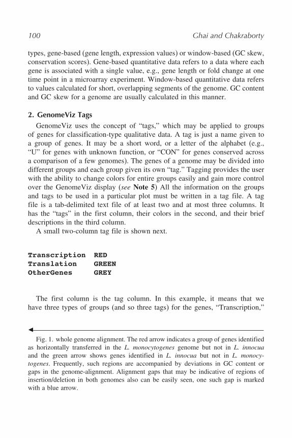
types, gene-based (gene length, expression values) or window-based (GC skew,conservation scores). Gene-based quantitative data refers to a data where eachgene is associated with a single value, e.g., gene length or fold change at onetime point in a microarray experiment. Window-based quantitative data refersto values calculated for short, overlapping segments of the genome. GC contentand GC skew for a genome are usually calculated in this manner.

2. GenomeViz TagsGenomeViz uses the concept of “tags,” which may be applied to groups

of genes for classification-type qualitative data. A tag is just a name given toa group of genes. It may be a short word, or a letter of the alphabet (e.g.,“U” for genes with unknown function, or “CON” for genes conserved acrossa comparison of a few genomes). The genes of a genome may be divided intodifferent groups and each group given its own “tag.” Tagging provides the userwith the ability to change colors for entire groups easily and gain more controlover the GenomeViz display (see Note 5) All the information on the groupsand tags to be used in a particular plot must be written in a tag file. A tagfile is a tab-delimited text file of at least two and at most three columns. Ithas the “tags” in the first column, their colors in the second, and their briefdescriptions in the third column.

A small two-column tag file is shown next.

Transcription REDTranslation GREENOtherGenes GREY

The first column is the tag column. In this example, it means that wehave three types of groups (and so three tags) for the genes, “Transcription,”

�Fig. 1. whole genome alignment. The red arrow indicates a group of genes identified

as horizontally transferred in the L. monocytogenes genome but not in L. innocuaand the green arrow shows genes identified in L. innocua but not in L. monocy-togenes. Frequently, such regions are accompanied by deviations in GC content orgaps in the genome-alignment. Alignment gaps that may be indicative of regions ofinsertion/deletion in both genomes also can be easily seen, one such gap is markedwith a blue arrow.


“Translation,” and “OtherGenes.” The second column simply states the colorthat should be used for coloring each group.

To change the color of the genes involved in “Translation,” simply changethe text GREEN in the second column to say, BLUE. When the plot is reloaded,the new colors will be displayed.

However, a tag file may also have three columns, as shown next.

T orange transcriptionR blue translationM green cell motilityS violet signal transduction- grey function unknown

The third column can be used to describe the tag if we wish. Its purposeis to provide a more informative description. It is recommended that numbers(0, 1, 2, 3 � � �) not be used as tags. The character “–” can also be used as a tag.All these columns must be separated with a “single” tab character only.

When one has a large number of tags, then it is useful to have a short descriptionof the tag. The tag file can be displayed within GenomeViz to read the descriptionsanytime. A tag file with all the COG categories is provided with GenomeViz.

3. GenomeViz Map FileThe file that contains the actual data to be plotted is called the map file. This

has been designed to be a simple format that can be easily edited and modifiedby anyone manually or with a program.

A sample map file is shown next (first few lines from the genome of thehyperthermophilic archaeon Aeropyrum pernix genome).

1669695APE0001 - - 213 938 hypothetical proteinAPE0002 K - 938 1276 hypothetical proteinAPE0004 R - 1260 2174 hypothetical proteinAPE0006 - + 2261 2836 hypothetical proteinAPE0007 - + 3896 5440 hypothetical proteinAPE0009 P - 5774 6091 transport protein


The first line of the map file contains only a single column, and a singlevalue: the total number of bases in the genome, in this case, 1,669,695. Allother lines of the map file contain six tab-delimited columns. The six columnsare described next.

1. A gene identifier or a name. National Center for Biotechnology Information (NCBI)frequently uses a “Locus Tag” feature to describe bacterial gene identifiers. Forexample, APE0001 is the locus tag for the first gene in the A. pernix genome. Thelocus tag for each gene can be seen in the NCBI Gene database. There are somelimitations to this identifier. First, it must be only a single word. Second, it mustnot be entirely a number, e.g., 1, 10, 124, are all invalid gene identifiers. Third,it must be unique for the genome the user is trying to plot. All identifiers for thegenomes provided with GenomeViz follow these three basic rules.

2. The tag/value column. The second column contains the tag that has been appliedto this gene to make it a part of a group of genes. In the example previously listed,four types of tags are visible, “K”, “R”, “P”, and “–”. The colors for these tags (andfor others in the map file) must be described in the tag file. The second columncontains tags in this example because this is an example of a qualitative data file.A map file, which contained the gene lengths for example, would have, in place ofthe tags, integer values for each gene.

3. The strand column. This column simply denotes the strand on which the gene lies.There can be only two values for this column, “+” or “−”. No other values areacceptable.

4. Gene start. This column contains the location of the start of the gene feature.5. Gene end. This column contains the location of the end of the gene feature. Both

the gene start and gene end must be valid integer values.6. Description. The last column of the map file. It contains the description, annotation,

name of the gene, and any other text information.

The only difference between a qualitative data map file and a quantitative datamap file is the values in the second column. All other columns are identicalfor the same genome.

If there is any line in the map file that does not have six columns in thecorrect format, GenomeViz will show an error, point out the incorrect linenumber and the column, and stop the plotting. In such as case, one must identifythe error, correct it, and redo the plot again. The map file format is easy tomaintain and modify in simple text editors or spreadsheets, and the extensiveformat checking performed by GenomeViz before plotting helps identify andcorrect mistakes before they are incorporated in the plot. The map file alone issufficient for plotting numerical data, but both the map and tag files are neededto plot classification-type data. The type of data, qualitative or quantitative, isautomatically detected from the map file.


4. Plotting a Genome Circle4.1. Types of Plots Available in GenomeViz

It is possible to plot data in several ways with GenomeViz. Given next is alist of methods available for plotting.

1. Plotting classification style data (qualitative).

a. Two circles (+ and − strand separately).b. Single circle (both + and − strands as a single circle).

2. Plotting numerical data (quantitative).

a. Gradient style graph with two circles (+ and − strand separately).b. Gradient style graph with single circle (+ and − strands as a single circle).c. One-sided line graph (like a circular bar chart, useful for alignment data).d. Two-sided line graph (useful for GC content and GC skew).

4.2. Plotting Classification-Style Data

Both the tag and map files are needed to create a classification-style plotin GenomeViz. Follow the following steps to create a classification style dataplot in GenomeViz.

4.2.1. Loading a TAG File

1. Go to File in the Main menu.2. Select Load Tag File, and choose for which genome to be loaded a TAG file for

(Genome 1, 2, 3, � � � 8). Choose “Genome 1.”3. Browse to the location of a tag file (say the TAG file supplied with GenomeViz –

tagfiles/COGs.tag).4. Click Open. The tag file COGs.tag is now loaded and this is displayed in a small

frame below the main menu. The loaded tags are also shown in the text displayarea. Now follow the steps next to load a map file and create the plot.

4.2.2. Loading a MAP file

1. Go to File in the Main menu.2. Select “Load Map File 1.”3. Choose “Draw Two Circles.”4. Choose “Classification Style Graph.”5. Browse to the location of a map file (e.g., the map file supplied with Genome Viz

for Escherichia coli K12 in the samples/classification-data directory – Escherichia_coli_K12.map).


6. Click Open.7. The genome of E. coli K12 will be displayed (two circles for two strands) colored

in the COG colors (as specified in the tag file) as Genome 1.

4.3. Plotting Numerical Data

No tag files are needed for plotting numerical data. Only a map file containingquantitative data is sufficient. Follow the following steps to load a map filecontaining numerical data to create a plot.

1. Go to File in the Main menu.2. Select “Load Map File 1.”3. Choose “Draw Two Circles.”4. Choose “One Sided Line Graph.”5. Choose “Blue.”6. Browse to the location of a map file (e.g., the gc-content map file supplied with

GenomeViz for E. coli K12 in the gc-content-mapfiles directory).

The GC content of the E. coli K12 genome in the map file will be displayedas a one-sided line plot colored in blue.

5. Plot Navigation and Highlighting5.1. Using Mouse Over

In all plots, Mouse Over on any gene immediately displays all the informationabout the gene in the display areas just below the Main menu. The line numberin the map file, the gene identifier, the tag/value, strand, gene start, gene end,and description all are displayed.

5.2. Selecting Genes

Clicking on any gene in the plot highlights it in a color called the “SelectionColor.” The default Selection Color is yellow. The information on a selectedgene is also displayed in a text display area on the right side of the drawingarea. Right clicking on a gene deselects it.

5.3. Select COGs

One can select COG categories directly for each genome using this menuprovided they are available in the map file. Thus, Select COGs→Select COGsin Genome 3→K-transcription, selects all genes classified in the categoryTranscription in the Map file for Genome 3. It is possible to select differentcategories in the same genome in different colors by simply changing theselection color before selecting the category. However, it is advisable to use


a neutral background tag file, e.g., COGsGrayScale.tag, to provide a bettercontrast for the categories of the user’s choice. This tag file colors all COGcategories in a neutral gray color. The user may also edit this tag file to reflectany other color as well.

5.4. Searching for Genes of Interest

The complete information in the map file can be searched using the Searchoption. All genomes may be queried independently of one another. Go to Search→ Search Genome 1 (to search in the first genome). A Search window appears.Type in the term to search, and press “search” (see Note 6). After the search iscompleted, a pop-up window appears and lists how many results were found.These results can be examined in the text display area on the right hand side of thedrawing area. The search results may also be saved to a text file. In addition, all thegenes that matched the search pattern are highlighted in the GenomeViz plot inthe “Search Color.” Several different searches (each with a different search color)can be run on the same genome or the plot. In this manner, the search and highlightfunctionality provides one with a rapid overview of distribution of search termsover the genome. A global search function is also available, i.e., all the plottedgenomes may be searched at once for a single pattern. The results are displayedgenome-wise in the text display area.

5.5. Removing a Genome Circle

If there has been an error in plotting a genome circle, this particular circlecan be easily removed without affecting the rest of the plot. Navigate toClear→Genome 1, to remove the outermost circle. Choose File→Clear All, toreset the entire plot.

5.6. Plot Summary

To have a quick overview of which files have been used to create eachgenome circle, one can go to Summary→Plot Details to have look at a tablecontaining the names of all the tag files and map files being used for eachgenome circle in the plot.

5.7. Printing the Plot

It is possible to create publication quality plots with GenomeViz (see Note 4).Once the user is satisfied with the plot created and wants to finally print it, theuser can go to File→Print. A print dialog box appears with several options. Givethe dialog box time to complete its rendering of the print preview plot in the


small window. Choose the paper size and choose “Print to file” option. Providea name for an output file, e.g., myplot.ps. GenomeViz creates postscript outputfiles that can be easily read in by standard graphics programs, and convertedto a PDF if desired.

5.8. The Mask Genome Menu

The search function provides highlighting genes based on a pattern match,and the tag file allows genes to be colored based on the group in whichit belongs. To color genes on a numerical data plot, that do not share anycommon search pattern, it is not possible to color them using these options.However, individual genes of interest in both the classification-style plots andthe quantitative data plots are searchable and can be colored by using the specialmask genome menu. It is somewhat like a multiple search option, but with thefacility of coloring each result in a specific color. It has a simple format, a twocolumn tab-delimited format, as shown next. The first column is the gene ofinterest, and the second column specifies the color it should be displayed in.

Gene1 redGene2 blueGene3 yellow

The Gene1 will be red, Gene2 will be blue, and Gene3 will be yellow. Noformat checking is performed on the mask file. It must be ensured by the userthat the format is correct, all gene identifiers used are present in the map file,and that the colors are valid Tk colors.

6. Implementation6.1. Supported Platforms

GenomeViz has been tested to run successfully on Linux and Solarisoperating systems (see Note 7). Unix systems that have ActiveTcl installedmay also run GenomeViz but we have not tested this.

6.2. ActiveTcl

It is required that the user install ActiveTcl distributed by ActiveState(http://tcl.activestate.com) to run GenomeViz. It is recommended over any otherexisting Tcl installation that the user might have to run GenomeViz. InstallingActiveTcl will not interfere with the user existing Tcl installation and will haveno effects on the user’s Tcl programs, if the user has any.


6.3. Perl

The user will also need Perl to run the scripts that are distributed withGenomeViz (see Note 8 ). Perl is usually installed by default on Linux/Unixsystems in the path/usr/bin/perl. The user can easily check this by typingthe following command on the terminal.which perlThe user may get/usr/bin/perlwhich means the user already has Perl installed, or the user may get

something likeperl not foundwhich means the user does not have Perl and will need to install it.If the user does need to install Perl, once again it is recommended that the

user gets the ActivePerl distribution from ActiveState. It is easy to install andshould not pose any difficulty.

7. Notes1. Use the Perl programs gc2viz and gcskew2viz to compute window-based mapfiles

for plotting in GenomeViz. They use only the nucleotide fasta file as inputand create a mapfile that can be plotted in GenomeViz. The GC content mapfiles supplied with GenomeViz contain only the GC content values of theactual genes themselves. The user can download whole genome nucleotide filesfor any sequenced bacteria genome from NCBI (http://www.ncbi.nlm.nih.gov/genomes/lproks.cgi). The nucleotide sequence files on the NCBI server have the“.fna” file extension.

2. A common application involves a list of genes that one would like to plot andvisualize along with other data. The script “tagit” makes it simple for to create afile that can be plotted and visualized easily with GenomeViz. Suppose the userhas a list of genes that the user is interested in. The user should provide the scriptwith the file containing this gene list and the tag the user wants to attach to thesegenes. The user should also provide the map file to be used (currently GenomeVizprovides 120 map files to choose from). The script creates a new map file, butwith all the genes tagged with the designated custom tag the user provides.

3. Whole genome alignments provide us information on which regions of the genomeshave been conserved and which have been subject to deletion and insertions. Itis easy to get complete genome alignments of bacterial genomes using AVID.Avid also provides a simple format for the representation of such alignments. Thescript avid2viz can reformat genome alignment data from the AVID program to amap file format that can be plotted in GenomeViz. This map file can be used tovisualize conservation data of genomes along with other data such as GC content,Basic Local Alignment Search Tool scores, and so on in GenomeViz.


4. Once a plot has been made, it should be saved to a postscript file. However, whenthe plot needs to be recreated, one needs to use the same input files once again.Use the Summary→Plot details to save the details of the files used to create theuser’s plot in such a case.

5. There are many different ways to specify the colors in the tag file. The colors ina tag file may be written by their name, e.g., Red, red, or RED are all acceptable.Hexadecimal codes are also allowed. Two color browsers are provided withinGenomeViz that can help to select colors and obtain their standard names orhexadecimal codes.

6. The search box supports advanced pattern matching abilities provided by theTcl/Tk regexp. For example, if the user wants to search for genes containing thepattern tRNA or rRNA, the user can type tRNA�rRNA, where the “�” characterdenotes OR. A link to a complete guide for regular expression pattern matchingusing Tcl can be found at the GenomeViz homepage.

7. GenomeViz and accompanying scripts and data can be download at theGenomeViz homepage (http://www.uniklinikum-giessen.de/genome/).

8. If the user can program in Perl, it is easy to modify the scripts provided withGenomeViz to create new programs that can compute parameters using a window-based approach, e.g., dinucleotide content, complexity, and so on.

AcknowledgmentsThe work reported herein is supported by grants from the Deutsche

Forschungsgemeinschaft and the BMBF Network Program Pathogenomics toTC. RG is supported by the Graduate College of Biochemistry of NucleoproteinComplexes (GK370), Justus Liebig University, Giessen, Germany.

References1. Kerkhoven, R., van Enckevort, F. H., Boekhorst, J., Molenaar, D., and Siezen, R. J.

(2004) Visualization for genomics: the Microbial Genome Viewer. Bioinformatics20, 1812–1814.

2. Sato, N. and Ehira, S. (2003) GenoMap, a circular genome data viewer.Bioinformatics 19, 1583–1584.

3. Leader, D. P. (2004) BugView: a browser for comparing genomes. Bioinformatics20, 129–130.

4. Gibson, R. and Smith, D. R. (2003) Genome visualization made fast and simple.Bioinformatics 19, 1449–1450.

5. Stothard, P. and Wishart, D. S. (2005) Circular genome visualization and explorationusing CGView. Bioinformatics 21, 537–539.

6. Ghai, R., Hain, T., and Chakraborty, T. (2004) GenomeViz: visualizing microbialgenomes. BMC Bioinformatics 5, 198.

7. Merkl, R. (2004) SIGI: score-based identification of genomic islands. BMCBioinformatics 5, 22.

Comparative Microbial Genome Visualization Using GenomeViz

Documents