Compact boson stars in K field theories

arX

iv:0

908.

0218

v2 [

hep-

th]

16 S

ep 2

009

Compact boson stars inK field theories

C. Adama∗, N. Grandib∗∗, P. Klimasa∗∗∗, J. Sánchez-Guilléna†, and A.Wereszczynskic††

a)Departamento de Fisica de Particulas, Universidad de Santiagoand Instituto Galego de Fisica de Altas Enerxias (IGFAE)

E-15782 Santiago de Compostela, Spainb) IFLP-CONICET

cc67 CP1900, La Plata, Argentinac)Institute of Physics, Jagiellonian University,

Reymonta 4, 30-059 Kraków, Poland

Abstract

We study a scalar field theory with a non-standard kinetic term mini-mally coupled to gravity. We establish the existence of compact boson stars,that is, static solutions with compact support of the full system with self-gravitation taken into account. Concretely, there exist two types of solutions,namely compact balls on the one hand, and compact shells on the other hand.The compact balls have a naked singularity at the center. Theinner boundaryof the compact shells is singular, as well, but it is, at the same time, a Killinghorizon. These singular, compact shells therefore resemble black holes.

∗[email protected]∗∗[email protected]∗∗∗[email protected]†[email protected]††[email protected]

1 Introduction

This paper investigates self-gravitating compact solutions of a non-linear scalarfield theory with a non-canonical kinetic term. Recently it has been establishedthat relativistic non-linear field theories may have static(solitonic) solutions withcompact support, such that the fields take their vacuum values identically outsidea compact region. Solitons of this type are called "compactons". At the moment,there are two known classes of field theories which may have compacton solu-tions. One possibility is that the (scalar) field of the theory has a potential witha non-continuous first derivative at (some of) its minima, a so-called V-shapedpotential [1] - [10]. The other possibility consists in a non-standard kinetic term(higher than second powers of the first derivatives) in the Lagrangian [11], [12], aso-called K field theory. It may be interesting to mention at this point that K fieldtheories have found some applications already in cosmologyas a candidate fordark energy, where theories of this type are known as "K essence", or "general-ized dynamics", see, e.g., [13] - [18]. They have been also applied to topologicaldefect formation, see, e.g., [19], [20].

In both cases of V-shaped potentials and of K theories, respectively, the expo-nential approach to the vacuum typical for conventional solitons is replaced by apower-like approach. Further, the vacuum value is reached at a finite distance (the"compacton boundary"), and the second derivative of the field is non-continuousat the compacton boundary. In some cases, the compacton solutions are, therefore,weak solutions (i.e., they do not solve the field equations atthe boundary) which,in these cases, is not problematic, because the space of weaksolutions is the ade-quate solution space for the corresponding variational problem. When gravitationis included, the stronger continuity requirements for a space-time manifold mightrender such a behaviour problematic, so let us emphasize already at this point thatthis does not happen for the self-gravitating compact solutions considered in thispaper, i.e., all solutions are strong solutions of the Einstein equations.

Like in the case of conventional solitons, for compactons itis also much sim-pler to find solutions in theories in 1+1 dimensions. We remark that for somenon-relativistic theories (generalizations of the KdV equations) compactons werealready found in [21], [22]. The most direct generalizationof topological com-pactons to higher dimensions faces the same problems like inthe case of con-ventional solitons, and also one possible solution is the same, namely the in-troduction of additional gauge fields, like in the case of vortices and monopoles[23]. Other possibilities to find higher-dimensional compactons consist in choos-ing more complicated topologies for the target space [24] orin allowing for a

1

simple time dependence in the form of Q balls [6], [7].A further natural question to be asked is whether these compactons may be

coupled to gravity and whether such self-gravitating compactons lead to some in-teresting applications. A first application has been to brane cosmology, wherethe self-gravitating compactons provide a model for a thickbrane with a strictlyfinite extension, as well as an automatic confinement of all matter fields to thebrane [25], [26], [27]. As this thick brane is of the domain wall type, the resultingsystem is essentially a one-dimensional problem. The coupling of the 3+1 di-mensional compact Q balls of the V-shaped class of models of [7] to gravity wasrecently studied in [28] mainly using numerical methods.

It is the main purpose of the present paper to study in detail the coupling ofa 3+1 dimensional radially symmetric compacton of a K field theory (with non-standard kinetic term) to gravity. For solutions to a scalarfield plus gravity theorythe notion of a "boson star" has become standard in the literature, therefore wewill call generic solutions of our model "compact boson stars", and reserve morespecific terms ("compact balls", or "singular shells") for the different types ofsolutions we shall encounter. For boson stars with a conventional kinetic term ofthe scalar field, there already exists a large amount of literature. Here one firstcriterion for a classification is whether the scalar field is real or complex. In thecase of a real scalar field, a static, spherically symmetric metric requires a static,spherically symmetric scalar field. The resulting field equations are known not tosupport solutions when gravity is neglected, because theirexistence is forbiddenby the Derrick theorem. For the corresponding system with gravity included, finite(asymptotic) mass solutions do exist, but they are beset by naked singularities,see e.g. [29] - [32]. For a complex scalar field, the Q-ball type ansatzφ(x) =exp(−iωt)f(r) still is compatible with a static, spherically symmetric metric. Inaddition, this ansatz allows for regular, finite energy solutions already in the casewithout gravity. As a consequence, regular finite mass solutions for the full systemwith gravity included do exist and have been widely studied,see e.g. [33] - [35].Reviews on boson stars may be found, e.g., in [36] - [38]. We remark that thesystem studied in the present paper is different in this respect, because, due to thenon-standard kinetic term, static finite energy solutions in the non-gravitationalcase are not excluded by the Derrick theorem, and they do indeed exist, as weshall see in the next section.

Our paper is organized as follows. In a first step, in Section 2we introducethe simplest K field theory which gives rise to non-topological compact balls inflat Minkowski space (i.e., without gravity). We discuss general features of theresulting compact ball solutions and calculate some explicit solutions by numer-

2

ically integrating the ODE for spherically symmetric compact balls. In Section3, we couple the model of the previous section to gravity via the usual, minimalcoupling. We derive the Einstein equations for sphericallysymmetric configura-tions and discuss in detail their properties. We then present some explicit compactboson star solutions by numerically integrating the ODEs for the spherically sym-metric configurations, and, finally, we investigate the singularities which form inthese solutions. We find, in fact, two types of solutions which have two differenttypes of singularities. The first type has naked, point-likesingularities and is, thus,consistent with the "no scalar hair" conjecture. The secondtype has a surface-likesingularity that is, at the same time, a singular boundary ofspace-time, and the lo-cus of a (Killing) horizon. This second type of solution, therefore, exhibits somesimilarity with a black hole. Section 4 contains a discussion of these results aswell as some speculations about possible astrophysical or cosmological applica-tions of compact boson stars of the type studied in this paper.

2 The non-gravitational case

We want to study the simplest possible scalar field theory in3+1 dimensions witha quartic kinetic term and a standard potential which gives rise to the formationof non-topological compact solitons (i.e. compactons). Therefore we choose theLagrangian

L = −X|X| − V (φ), (1)

where

X =1

2gµν∂µφ∂νφ, V (φ) = λφ2. (2)

We remark that, in the case at hand, the Derrick scaling stability criterion doesnot exclude the existence of static solutions, thanks to thenon-standard, quartickinetic term. The absolute value symbol in the kinetic term is necessary to ensureboundedness from below of the energy. For static configurations this absolutevalue symbol is immaterial in the case without gravity, because the metric func-tions are given functions with a fixed sign. For the case with gravitation includedthis is not guaranteed a priori because the metric functionshave to be determinedfrom the Einstein equations and could, in principle, changesign (as happens, e.g.,in the case of the Schwarzschild solution). We will find, however, that such a signchange is not possible in our model.

3

The line elementds2 of flat spacetime in spherical polar coordinates reads

ds2 = −dt2 + dr2 + r2(dθ2 + sin2 θdφ2) (3)

Now we assume spherical symmetryφ = φ(r) then the Euler-Lagrange equationtakes the form

1

r2

(

r2φ′3)′ − 2λφ = 0. (4)

It is convenient to introduce the new variables = r1/3 instead ofr. In the variables equation (4) takes the form

φ′2φ′′ − 54λs8φ = 0. (5)

The advantage of the new variables is that solutions have a power series expansionabout zero in the variables, but not inr. We remark that this will no longer holdin the case with gravitation included. There solutions willhave a regular powerseries expansion aboutr = 0 in the variabler. For brevity, in the sequel we shallcall the variables "radius", as well, and distinguish the two variables only bytheirrespective letters.1

2.1 Expansion at the boundary

As always in the case of compactons, we now assume that there exists a certainradiuss = S where the field takes its vacuum value, and its first derivative van-ishes. Further, the second derivative is nonzero from below(for s < S), whereasit is zero fors > S (such thatφ takes its vacuum value zero fors > S). Indeed,expandingφ(s) arounds = S,

φ(s) =∑

j

fj(s− S)j for s < S (6)

and assuming thatφ(s = S) = φ′(s = S) = 0 we get a cubic equation forf2 withthe three solutions

f2 = (0,±3

2

√3λS4). (7)

1We remark that, in addition to the compacton solutions discussed below, Eq. (5) has the iso-lated (i.e., without free integration constants) analytical solutionφ = ±

√

λ/20s6. This solutiongrows without bound for increasings and, obviously, cannot give rise to a finite energy configura-tion.

4

If we further assume, without loss of generality, thatφ takes the positive valuef2 = +(3/2)

√3λS4 for s < S and the vacuum valuef2 = 0 for s ≥ S then the

higher coefficientsfj are uniquely determined by linear equations and we find theexpansion

φ(s) =3

2

√3λS4(s− S)2 +

12

5

√3λS3(s− S)3 +

2√

3λS2(s− S)4 + O((s− S)5) for s < S

φ(s) = 0 for s ≥ S. (8)

We remark that also in ther variable the functionφ(r) approaches its vacuumvalue quadratically atr = R ≡ S3, because the conditionsφ(S) = φ′(S) = 0 areinvariant under a variable change. Indeed, we find

φ(r) =1

2

√

λ

3(r − R)2 − 1

15R

√

λ

3(r − R)3 +

13

270R2

√

λ

3(r − R)4 + O((r − R)5), for r < R

φ(r) = 0 for r ≥ R.

2.2 Expansion at the center

Plugging a Taylor series expansion arounds = 0 into eq. (5) we find that thefirst two coefficientsφ(s = 0) ≡ φ0 andφ′(s = 0) ≡ α remain undetermined,whereas the higher ones are determined uniquely by linear equations. Due to thestrong suppression factors8 at the r.h.s. of eq. (5) we find that the coefficients ofs2 to s9 are, in fact, zero. Concretely we find

φ(s) = φ0 + αs+3φ0

5α2λs10 +

27

55αλs11 + O(s19). (9)

The three next higher order termsO(s19)−O(s21) include only terms proportionalto λ2.

2.3 Compact ball solutions

We shall find solutions explicitly by numerical integration. But before performingthese calculations we want to discuss some generic featuresof eq. (5) which allow

5

to establish both the existence and several properties of these compact ball solu-tions. A first indication for the existence of solutions can be found by counting thenumber of boundary conditions and free parameters in the numerical integration.There are two possibilities for the numerical integration,namely a shooting fromthe center, or a shooting from the boundary. If we shoot from the center, thereare altogether three free parameters, namelyφ(0) ≡ φ0, φ′(0) ≡ α, and the com-pacton radiusS. On the other hand, there are two boundary conditions that have tobe obeyed for a compacton, namelyφ(S) = φ′(S) = 0. Therefore, we expect theexistence of a one-parameter family of compact balls which may be parametrized,e.g., by the compacton radiusS. If we shoot from the compacton boundary, theonly free parameter is the compacton radiusS. On the other hand, there are noboundary conditions ats = 0, because bothφ(0) andφ′(0) are undetermined bythe expansion ats = 0. So again we expect a one-parameter family of solutions.

Further conclusions may be drawn by a closer inspection of eq. (5). Firstly,we observe that eq. (5) is invariant under the reflectionφ → −φ. Thereforewe may chooseφ0 ≡ φ(0) > 0 without loss of generality. Secondly, it followsimmediately from eq. (5) that away from the center (i.e. fors > 0) it holds thatif φ > 0 thenφ′′ > 0. As a consequence, ifφ0 > 0 andα ≡ φ′(0) > 0 thenthe scalar fieldφ will grow indefinitely and may never reach its vacuum valueφ = 0. We conclude that a compact ball requiresα < 0. Now for genericα < 0the following may happen. If for a fixed value ofφ0 the slope is too weak (i.e.if |α| is too small) thenφ(s) will reach a points0 whereφ′(s0) = 0 before itreachesφ = 0. At this points0 the second derivativeφ′′ (and, consequently, allhigher derivatives) becomes singular and the integration breaks down. On theother hand, if|α| is too big, thenφ will cross the lineφ = 0 instead of touchingit, and then develop towards more and more negative values ofφ indefinitely. Itfollows that there exists an intermediate value ofα such thatφ touches the lineφ = 0 instead of crossing it. This is the compact ball solution, and the points = Swhere the touching occurs is the compacton radius.

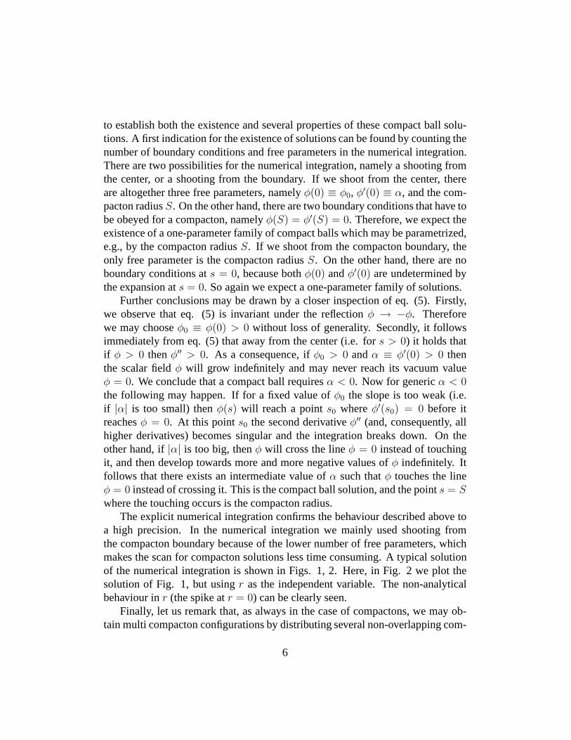
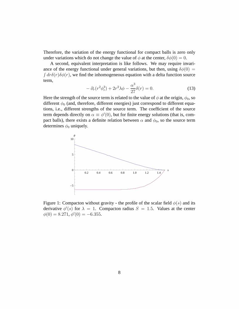
The explicit numerical integration confirms the behaviour described above toa high precision. In the numerical integration we mainly used shooting fromthe compacton boundary because of the lower number of free parameters, whichmakes the scan for compacton solutions less time consuming.A typical solutionof the numerical integration is shown in Figs. 1, 2. Here, in Fig. 2 we plot thesolution of Fig. 1, but usingr as the independent variable. The non-analyticalbehaviour inr (the spike atr = 0) can be clearly seen.

Finally, let us remark that, as always in the case of compactons, we may ob-tain multi compacton configurations by distributing several non-overlapping com-

6

pactons with different centers in flat space.

2.4 Energy functional

We found that there exist compact ball solutions for arbitrary values of the fieldat the centerφ0 (or, equivalently, for arbitrary valuesS of the compacton radius),and it is easy to see that these different values ofφ0 correspond to different valuesof the total energy. Therefore, compact balls do not correspond to genuine criti-cal points of the energy functional, and one may wonder why solutions do existat all. There are two possible ways to understand this puzzle. Starting from thereduced energy functional for radially symmetric fields, the answer is that varia-tions of the energy functional may receive contributions from the boundary, and itis precisely these variations of the boundary which give nonzero contributions tothe energy functional for a compact ball solution. The second, equivalent answeris that the compact balls solve an inhomogeneous equation with a delta functionsource term. This we want to demonstrate explicitly in the sequel. In a first step,we write down the energy functional and then use the principle of symmetric crit-icality to rewrite this energy functional as a functional for radially symmetric fieldconfigurations (the principle of symmetric criticality just states that this reductionof the energy functional to radially symmetric configurations provides the correctradially symmetric field equations if the field equations arecompatible at all withthis symmetry reduction - i.e., with the ansatzφ = φ(r)). We get

E[φ] =∫

r2dr sin θdθdϕ(

1

4((∇φ)2)2 + λφ2

)

= 4π∫ ∞

0r2dr

(

1

4φ4

r + λφ2)

. (10)

For the variation of the functional we find

δE = 4π∫ ∞

0r2dr

(

φ3rδφr + 2λφδφ

)

= 4π∫ ∞

0dr(

−∂r(r2φ3

r) + 2r2λφ)

δφ

+4π(r2φ3rδφ)|R0 (11)

where we performed a partial integration and used the fact thatφ is a compact ballsolution which takes its vacuum value forr ≥ R. Using the smallr behaviourφ(r) ∼ φ0 + αr

1

3 we finally get for the boundary term

4π(r2φ3rδφ)|R0 = −4π

α3

27δφ(0). (12)

7

Therefore, the variation of the energy functional for compact balls is zero onlyunder variations which do not change the value ofφ at the center,δφ(0) = 0.

A second, equivalent interpretation is like follows. We mayrequire invari-ance of the energy functional under general variations, butthen, usingδφ(0) =∫

drδ(r)δφ(r), we find the inhomogeneous equation with a delta function sourceterm,

− ∂r(r2φ3

r) + 2r2λφ− α3

27δ(r) = 0. (13)

Here the strength of the source term is related to the value ofφ at the origin,φ0, sodifferentφ0 (and, therefore, different energies) just correspond to different equa-tions, i.e., different strengths of the source term. The coefficient of the sourceterm depends directly onα ≡ φ′(0), but for finite energy solutions (that is, com-pact balls), there exists a definite relation betweenα andφ0, so the source termdeterminesφ0 uniquely.

0.2 0.4 0.6 0.8 1.0 1.2 1.4s

-5

0

5

10Φ

Figure 1: Compacton without gravity - the profile of the scalar field φ(s) and itsderivativeφ′(s) for λ = 1. Compacton radiusS = 1.5. Values at the centerφ(0) = 8.271, φ′(0) = −6.355.

8

0.5 1.0 1.5 2.0 2.5 3.0r0

2

4

6

8

Φ

Figure 2: Compacton without gravity - the profile of the scalar field of Figure 1,but expressed in the variabler = s3, φ(r). Compacton radiusR = S3 = 3.375.

3 The model with gravity

We now consider the scalar field model of the previous sectioncoupled minimallyto gravity. The action reads

S =∫

d4x√

|g|(

1

κ2R−X|X| − V (φ)

)

, (14)

where, as before,

X =1

2gµν∂µφ∂νφ, V (φ) = λφ2. (15)

Further,R is the curvature scalar, andg is the determinant of the metric tensor.We now assume a spherically symmetric space time, then the line elementds2

may be chosen in the form

ds2 = −A(r)dt2 +B(r)dr2 + r2(dθ2 + sin2 θdφ2) (16)

where for consistency we have to assume thatφ = φ(r) depends on the radialcoordinater only. The Euler-Lagrange equation forφ(r) takes the form

(

|B−1|B−1φ′3)′

+

(

2

r+

1

2

(

A′

A+B′

B

))

|B−1|B−1φ′3 − 2λφ = 0. (17)

9

The Einstein equations may be obtained from the Einstein tensor, which has theindependent components

G00 = A(

(rB2)−1B′ +1

r2(1 − B−1)

)

, (18)

G11 = B(

(rAB)−1A′ − 1

r2(1 −B−1)

)

, (19)

G22 = r2(

1

2(AB)−1/2((AB)−1/2A′)′ +

1

2(rAB)−1A′ − 1

2(rB2)−1B′

)

(20)

(G33 is not independent but obeysG33 = sin2 θG22), and the energy-momentumtensor

Tµν = − ∂L∂(∂µφ)

∂νφ+ gµνL

= 2|X|∂µφ∂νφ− gµν(|X|X + λφ2) (21)

with the independent components

T00 = A(

1

4|B−1|B−1φ′4 + λφ2

)

, (22)

T11 = |B−1|φ′4 −B(

1

4|B−1|B−1φ′4 + λφ2

)

, (23)

T22 = −r2(

1

4|B−1|B−1φ′4 + λφ2

)

. (24)

The Einstein equations read

B′ =1

rB(1 − B) + κ2rB2

(

1

4|B−1|B−1φ′4 + λφ2

)

, (25)

A′

A=

1

r(B − 1) +

3

4κ2r|B−1|φ′4 − κ2λrBφ2, (26)

1

2(AB)−1A′′ − 1

4(AB)−2(AB)′A′ +

1

2(rAB)−1A′ − 1

2(rB2)−1B′ +

+κ2(

1

4|B−1|B−1φ′4 + λφ2

)

= 0. (27)

Here several comments are appropriate. Firstly, there seemto be four equations(the field equation (17) and the three Einstein equations) for three real functionsφ, A andB. As always in the case of one real scalar field, these equations are,

10

however, not independent. The field equation may, in fact, bederived from thethree Einstein equations. Further, in the case at hand, the field equation (17) maybe derived from the three Einstein equations in a purely algebraic fashion (i.e.,without performing additional derivatives). This followseasily from the fact thatboth the field equation (17) and the third Einstein equation (27) are of secondorder. Therefore, the field equation and the third Einstein equation are completelyequivalent, at least in non-vacuum regions whereφ′ 6= 0 (in regions whereφ′ =0 the field equation is more restrictive, because its derivation from the Einsteinequations requires a division byφ′). We remark that the above feature is notalways true (in some cases the Einstein equations are more restrictive and have tobe used, because the derivation of the field equations involves further derivatives).

Secondly, the functionA appears in all equations only in the combination(A′/A) and derivatives thereof (this is also true for Eq. (27), where it is not com-pletely obvious). Therefore, one may eliminate the functionAwith the help of Eq.(26) from all the remaining equations. One may choose a set oftwo independentequations inφ andB from these remaining equations, solve them forφ andB,and determine the correspondingA from Eq. (26) in a second step. It is obviousfrom Eq. (26) thatA is determined up to a multiplicative constant. The choice ofthis constant just corresponds to a constant rescaling of the time coordinate. Thisconstant will be fixed by the condition that asymptotically (that is, forr biggerthan the compacton radiusR ), the metric is equal to the Schwarzschild metric,i.e.,

A(r) = B−1(r) = 1 − Rs

rfor r > R > Rs (28)

(we will find that the compacton radius is always bigger than the Schwarzschildradius,R > Rs, and that a horizon never forms). Concretely, for the two indepen-dent equations forB andφ we choose Eq. (25) forB and the field equation Eq.(17) forφ, where we eliminate both(A′/A) andB′ from the latter equation withthe help of Eqs. (26) and (25). It will be useful for our discussion to display theresulting system of two equations again. We get

B′

B=

1

r(1 −B) + κ2r

(

sign(B)

4Bφ′4 + λBφ2

)

(29)

for B and

3φ′2φ′′ = 2(

κ2λrφ2B − B

r

)

φ′3 + 2λsign(B)B2φ (30)

for φ (heresign(B) ≡ (|B|/B) is the sign function). We remark for later use thatif we forget about the sign function, then the equations for negativeB may be

11

recovered from the equations for positiveB by the combined coupling constanttransformations

λ→ −λ , κ2 → −κ2. (31)

3.1 Qualitative behaviour ofB

Before starting the numerical investigation and the expansions at the compactonboundary and at the center, we want to draw some conclusions on the behaviourof the functionB. Concretely, we want to show that for a nonsingular scalar fieldφ, B(r) cannot approach zero from the inside, that is, from smaller values ofr.This implies that whenB(r) takes the value zero at some radiusr = r0, thenB(r) is not defined forr < r0. Differently stated, if we start the integration atsome valuer > r0 whereB(r) > 0 (this we assume because we want to connectto the Schwarzschild solution), and we then integrate downwards (i.e. towardssmaller values ofr), then the integration breaks down atr = r0. We shall find inthe sequel that at this value a singularity forms, that is, some curvature invariantsbecome infinite atr = r0. Here we have to distinguish two cases, namelyr0 = 0or r0 > 0. In the caser0 = 0 the singularity is just a point at the origin of ourcoordinate system, whereas forr0 > 0 the locus of the singularity is a two-sphereS2, so space has a singular boundary withS2 topology. We shall call solutionsof the first type "compact balls" in the sequel, whereas the second type (with thesingular inner boundary ofS2 shape) are called "singular shells". We discuss thisbehaviour here because it is precisely what is found in the numerical integration(that is, if we start at some compacton boundaryr = R and then integrate towardssmallerr, B will always hit the lineB = 0, either atr = 0 or at some nonzeror = r0).

It remains to demonstrate thatB cannot be continued to the regionr < r0. IfB > 0 for r > r0 and approaches zero atr = r0, then necessarily(B′/B) > 0for r > r0 but sufficiently close tor0. A continuation tor < r0 may either crosszero, in which caseB < 0 andB′ > 0 for r < r0 but sufficiently close tor0.Or the continuation may return to the regionB > 0 for r < r0, in which caseB > 0 andB′ < 0 for r < r0 but sufficiently close tor0. In both cases the ratiobetweenB′ andB is negative,(B′/B) < 0 for r < r0 but sufficiently close tor0.The inequality(B′/B) < 0 is, however, incompatible with Eq. (29) forr < r0and sufficiently close tor0. In fact, the r.h.s. of Eq. (29) is manifestly positivefor r close tor0. The first term(1/r)(1 − B) ∼ (1/r) is positive and not small.The second term,κ2r(φ′4/4|B|), is positive, and its magnitude depends onφ. Thethird term,κ2λrBφ2, may change sign if we assume thatB does. It is, however,

12

small nearr0, because it is proportional toB itself. The conclusion is that theratio (B′/B) is always positive nearr = r0 and, therefore,B cannot be continuedto valuesr < r0.

In a next step, we want to prove that a Schwarzschild type horizon ofB is im-possible for compacton solutions, too. We remind the readerthat the Schwarzschildsolution forB is

BS =(

1 − Rs

r

)−1

=r

r − Rs

=Rs

ǫ+ 1 , ǫ ≡ r −Rs. (32)

For a Schwarzschild type horizon coordinate singularity we, therefore, expand

B(ǫ) =Rs

ǫ+

∞∑

n=0

bnǫn

φ(ǫ) =∞∑

n=0

fnǫn (33)

We now insert this expansion into Eq. (30) where we assume at the moment thatr > Rs, that is,ǫ > 0 and, therefore,B > 0. Eq. (30) then becomes

3φ′2φ′′ = 2(

κ2λ(Rs + ǫ)φ2B − B

Rs + ǫ

)

φ′3 + 2λB2φ (34)

and we immediately find thatf0 = 0 because otherwise the coefficient ofǫ−2 inEq. (34) cannot be set to zero. Forf1 we find a cubic equation with the threesolutions

f1 = (0,±Rs

√λ) (35)

For f1 = 0 it follows easily that all the higherfi are zero, as well, so thatφ ≡ 0takes its vacuum value everywhere, and we are back to the Schwarzschild solutionB = BS for the metric functionB. For non-zerof1 we may choose the positiveroot f1 = Rs

√λ without loss of generality. This choice corresponds to a formal

solution, but the resulting scalar fieldφ grows without bound for increasingǫ, asfollows easily from Eq. (34). Indeed,φ can avoid unbound growth only ifφ′ = 0somewhere in the regionǫ > 0, butφ′ = 0 implies2λB2φ = 0 which is impos-sible (φ is nonzero at its maximum by assumption, whereasB cannot approachzero in the direction of growingr, as we know from the last paragraph). Specif-ically, the formal solution for nonzerof1 can, therefore, never join a compactonwith its compacton boundary somewhere in the regionr > Rs. Reversing theargument, we conclude that a horizon of the Schwarzschild type can never formfor a compact ball solution.

13

We still want to know what happens near a Schwarzschild type horizon forr < Rs, i.e.,ǫ < 0. ThereB < 0, and we remind the fact that solutions forB < 0may be inferred from solutions forB > 0 by the coupling constant transformation(31), specificallyλ → −λ. We therefore find for the linear coefficientf1 =

(0,±iRs

√

λ), and obviously only the trivial vacuum solutionf1 = 0 ⇒ φ = 0is real and, therefore, physically acceptable. We concludethat the only possiblefield configuration inside a horizon is the vacuum configurationφ ≡ 0. We mightstill ask what happens if we try to put a compacton strictly inside the horizon, thatis, at a compacton radiusR < Rs. We will find that the result is the same, i.e.,the nontrivial expansion coefficients forφ become imaginary, and only the trivialvacuum configurationφ ≡ 0 is possible inside the horizon.

We conclude that for compact boson star solutions the functionB can neverbe negative,B ≥ 0.

3.2 Behaviour at the boundary

Now we assume the existence of a compact boson star boundary,that is, a radiusr = R whereφ(R) = φ′(R) = 0, whereas the second derivative is zero fromabove but nonzero from below. Assuming thatB is nonnegative (because wewant to smoothly join it to the Schwarzschild solution forr > R), and pluggingthe power series expansions aroundr = R

φ(r) =∑

k=2

fk(r − R)k, (36)

B(r) =∑

k=0

bk(r −R)k, (37)

into (29) and (30) gives

f2 = 0,±1

2

√

λ

3b0

f3 = 0,∓ 1

15R

√

λ

3b0(4b0 − 3)

f4 = 0,± 1

270R2

√

λ

3b20(47b0 − 34)

. . .

b1 = −b0R

(b0 − 1),

14

b2 =b20R2

(b0 − 1),

b3 = − b30R3

(b0 − 1),

. . .

As expected, we find three roots forf2, so the vacuum solutionf2 = 0 for r > Rmay be smoothly joined to one of the two nontrivial roots off2 at r = R. In thesequel we choose the positive rootf2 = (1/2)

√

λ/3b0 without loss of generality.We remark that for negativeB the nonzero roots of the coefficientf2 becomeimaginary, as already announced in the previous section.

Inserting, further, the power series expansions above and the one forA,

A(r) =∞∑

k=0

ak(r − R)k (38)

into Eq. (26) forA we get

a1 =a0

R(b0 − 1),

a2 = − a0

R2(b0 − 1),

a3 =a0

R3(b0 − 1),

. . .

For the expansion coefficients ofB andA we, therefore, find that also for nonzerofk, the leading behaviour ofA(r) andB(r) close tor = R is like for the vacuum(i.e., Schwarzschild) solution. The first contribution of anonzerof2 appears ina6

and inb5. An easy way to see this is to study the power series expansionof theproductAB for r < R,

A(r)B(r) = a0b0 −R

45κ2λ2a0b

40(R− r)5 + O((R− r)6), (39)

where the positive nontrivial root off2 was inserted. Forr > R, A andB shouldform the Schwarzschild metric, which fixes the constanta0 to the valuea0 = b−1

0 .On the other hand,b0 is a free parameter which is related to the Schwarzschild ra-diusRs or to the asymptotic Schwarzschild massms = (Rs/2) of the asymptoticSchwarzschild metric, as well as to the compacton radius, via

b0 =(

1 − 2ms

R

)−1

. (40)

15

We find that the expansion at the compacton boundary leaves uswith two freeparameters, namelyb0 and the compacton radiusR. Equivalently, we may choosethe Schwarzschild massms ≡ Rs/2 and the compacton radius as free parameters.

Before studying the expansion from the inside, let us discuss briefly what toexpect for an integration which starts at the compacton boundary and proceedstowards smallerr. It holds that atr = R, B(R) > 1 andφ(R) = φ′(R) = 0,thereforeB′(R) is negative andB will at first increase towards smaller values ofr, see Eq. (29). For even smaller values ofr, the additional, positive terms atthe r.h.s. of Eq. (29) start to contribute, soB′ may become positive or negative,depending on the relative strength of the different terms atthe r.h.s. of Eq. (29).It turns out numerically that for a certain radiusB′ always becomes positive suchthatB starts to shrink towards smaller values ofr. OnceB has shrunk sufficientlysuch thatB < 1, then the r.h.s. of Eq. (29) is necessarily positive, such thatB hasno other choice than shrinking further. Numerically, this is exactly what happens,for all possible values of the two free parameters. Therefore, for sufficiently smallr, there are the following three possibilities for the behaviour ofB. It may shrinkto a nonzero value atr = 0, i.e.,B(r = 0) > 0. We will see that there exists onlyone isolated solution forB(0) > 0 (i.e., without free integration constants), andthis solution cannot be connected to a compacton boundary. Or B may go to zeroat r = 0, B(r = 0) = 0. We will see that two different kinds of solutions of thistype may be connected to a compacton boundary. They will formthe solutions ofthe compact ball type. The third possibility is thatB becomes zero already for anonzeror = r0, i.e.,B(r = r0 > 0) = 0. These are the singular shells.

3.3 Expansion at the center

In this section we assume that a solution exists locally nearr = 0. We insert thepower series expansions forφ andB

φ(r) =∑

k=0

fkrk, (41)

B(r) =∑

k=0

bkrk, (42)

into (29) and (30). In a first step we want to assume thatb0 > 0. Cancellation ofthe coefficient ofr−1 in Eq. (29) then requiresb0 = 1, whereas cancellation ofthe coefficients ofr−1 andr0 in Eq. (30) requiref0 = 0 andf1 = 0. All higherexpansion coefficients are uniquely determined (up to an overall sign ofφ), that

16

is, the solution is an isolated one without free integrationconstants. Explicitly, wefind (we choose the plus sign forφ)

φ(r) =

√λ√20r2 + O(r8)

B(s) = 1 +3κ2λ2

350r6 + O(r12) (43)

This solution behaves like at a compacton boundary already at the centerr = 0(i.e. φ(0) = 0, φ′(0) = 0), and the question is whether it can be connected toa compacton boundary at some nonzeror = R. It follows easily from Eq. (30)that this is impossible. Indeed, ifφ takes its vacuum valueφ = 0 at two differentradii, then it must pass through a local maximum at somer = r0 between the tworadii (whereφ(r0) > 0 andφ′(r0) = 0). But the existence of this maximum isincompatible with Eq. (30).

Therefore, we now assumeb0 = 0 and find

φ(r) = f0 + f1r −1

3b1f1r

2 +(

5

27b21f1 −

1

36κ2f 5

1

)

r3 + O(r4)

B(s) = b1r +(

1

4κ2f 4

1 − b21

)

r2 +(

b31 −7

12κ2b1f

41

)

r3 + O(r4). (44)

Here,f0, f1 andb1 are free parameters (integration constants). We remark that forcompact ball solutions (that is, for the correct matching toa compacton boundary)both f0 and f1 have to be nonzero. On the other hand, there will exist solutionswith b1 = 0. In this case the leading terms of the expansion read

φ(r) = f0 + f1r −κ2

36f 5

1 r3 +

κ4f 51 (5f 4

1 + 18λf 20 )

2160r5 + O(s6)

B(s) =κ2

4f 4

1 r2 − 7κ4f 8

1

144r4 +

κ6f 81 (4f 4

1 + 9λf 20 )

432r6 + O(r7) (45)

The power series expansion forA has to be treated independently forb1 6= 0 andb1 = 0, because the leading behaviour for smallr is completely different, beingA(r) ∼ r−1 for b1 6= 0, andA ∼ r2 for b1 = 0, as may be inferred easily from Eq.(26). Forb1 6= 0 the leading terms in the expansion read

A(r) = a−1

(

1

r+

(

b1 +3κ2f 4

1

4b1

)

+κ2f 4

1

16b21

(

4b21 + 3κ2f 41

)

r + O(r2)

)

(46)

17

whereas forb1 = 0 it reads

A(r) = a2

(

r2 − κ2f 41

12r4 +

κ4f 81

108r6 + O(r8)

)

(47)

The leading coefficientsa−1 or a2, respectively, are free parameters in the powerseries expansion. They appear as linear factors also in all higher coefficients, inaccordance with our observation thatA is determined up to a multiplicative con-stant. They cannot be determined from the local analysis atr = 0, but must insteadbe determined from the condition thatA approaches a Schwarzschild metric at thecompacton boundary.

3.4 Selfgravitating compact ball solutions

Before explicitly performing the numerical integration, we again want to deter-mine the number of free parameters and boundary conditions,both for a shootingfrom the boundary and for a shooting from the center. Here we only consider theparameters and boundary conditions forφ andB, because these two can be deter-mined from the system of two equations (29) and (30).Amay then be determinedfrom Eq. (26) in a second step, and we know already that the multiplicative con-stant which is the free parameter ofA must be determined by a matching to theSchwarzschild metric at the compacton boundary.

At the compacton boundary there are two free parameters, namely the com-pacton radiusR and the Schwarzschild (or asymptotic, ADM) massms. Con-cerning the conditions that have to be imposed at the centerr = 0, we have todistinguish the caseb1 6= 0 from the caseb1 = 0. In the caseb1 6= 0, there areno conditions imposed atr = 0, because the first two coefficientsf0 andf1 of φare unrestricted, and the fact thatb0 = 0 does not count as a boundary condition,because it is true for all generic solutions that exist locally nearr = 0 (we remindthe reader that the solution withb0 = 1 is an isolated solution with no free param-eters). We, therefore, expect a two-parameter family of solutions. Specifically, fora fixed Schwarzschild mass we expect to find a one-parameter family of compactball solutions with different radii. We shall call this typeof solutions withb1 > 0"large compactons" in the sequel.

In the caseb1 = 0, this condition provides exactly one boundary conditionat r = 0. In this case we, therefore, expect a one-parameter family of solutions.Specifically, for a fixed Schwarzschild massms we expect only one compact ballwith a fixed radius. We shall refer to this type of solutions as"small compactons".

18

An analysis of the shooting from the center leads to the same results. For thecaseb1 6= 0 (large compactons), there are four free parameters, namelyb1 itself,f0, f1, and the compacton radiusR. Further, there are two boundary conditions atthe compacton boundaryr = R, namely the conditionsφ(R) = 0 andφ′(R) = 0.Therefore, we expect a two-parameter family of compact ballsolutions. In thecaseb1 = 0 (small compactons), we are left with three free parametersf0, f1

andR and the same boundary conditions atr = R, therefore we expect a one-parameter family of solutions.

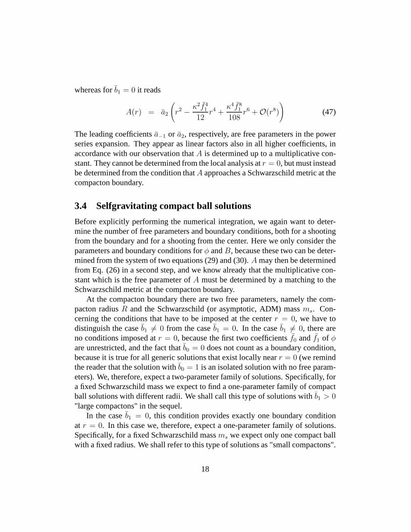
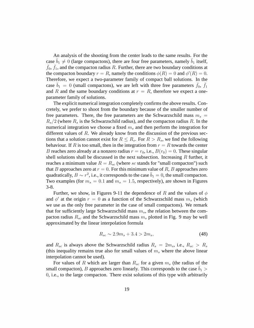
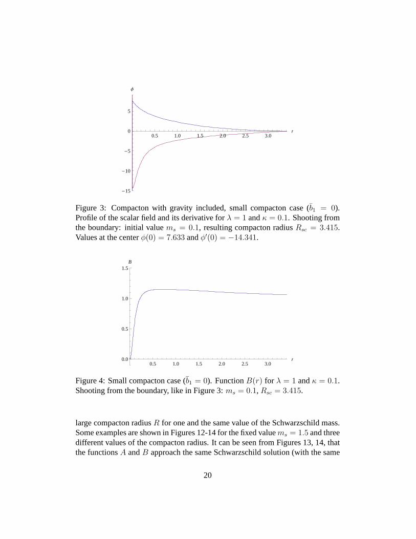
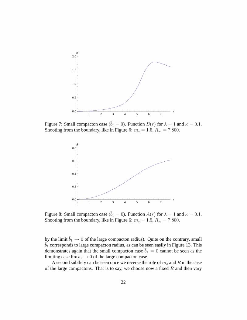
The explicit numerical integration completely confirms theabove results. Con-cretely, we prefer to shoot from the boundary because of the smaller number offree parameters. There, the free parameters are the Schwarzschild massms =Rs/2 (whereRs is the Schwarzschild radius), and the compacton radiusR. In thenumerical integration we choose a fixedms and then perform the integration fordifferent values ofR. We already know from the discussion of the previous sec-tions that a solution cannot exist forR ≤ Rs. ForR > Rs, we find the followingbehaviour. IfR is too small, then in the integration fromr = R towards the centerB reaches zero already at a nonzero radiusr = r0, i.e.,B(r0) = 0. These singularshell solutions shall be discussed in the next subsection. IncreasingR further, itreaches a minimum valueR = Rsc (wheresc stands for "small compacton") suchthatB approaches zero atr = 0. For this minimum value ofR,B approaches zeroquadratically,B ∼ r2, i.e., it corresponds to the caseb1 = 0, the small compacton.Two examples (forms = 0.1 andms = 1.5, respectively), are shown in Figures3-8.

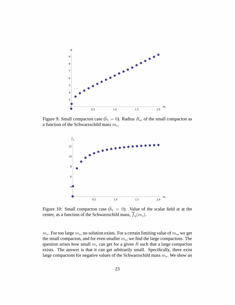
Further, we show, in Figures 9-11 the dependence ofR and the values ofφandφ′ at the originr = 0 as a function of the Schwarzschild massms (whichwe use as the only free parameter in the case of small compactons). We remarkthat for sufficiently large Schwarzschild massms, the relation between the com-pacton radiusRsc and the Schwarzschild massms plotted in Fig. 9 may be wellapproximated by the linear interpolation formula

Rsc ∼ 2.9ms + 3.4 > 2ms, (48)

andRsc is always above the Schwarzschild radiusRs = 2ms, i.e., Rsc > Rs

(this inequality remains true also for small values ofms where the above linearinterpolation cannot be used).

For values ofR which are larger thanRsc for a givenms (the radius of thesmall compacton),B approaches zero linearly. This corresponds to the caseb1 >0, i.e., to the large compacton. There exist solutions of thistype with arbitrarily

19

0.5 1.0 1.5 2.0 2.5 3.0r

-15

-10

-5

0

5

Φ

Figure 3: Compacton with gravity included, small compactoncase (b1 = 0).Profile of the scalar field and its derivative forλ = 1 andκ = 0.1. Shooting fromthe boundary: initial valuems = 0.1, resulting compacton radiusRsc = 3.415.Values at the centerφ(0) = 7.633 andφ′(0) = −14.341.

0.5 1.0 1.5 2.0 2.5 3.0r0.0

0.5

1.0

1.5B

Figure 4: Small compacton case (b1 = 0). FunctionB(r) for λ = 1 andκ = 0.1.Shooting from the boundary, like in Figure 3:ms = 0.1,Rsc = 3.415.

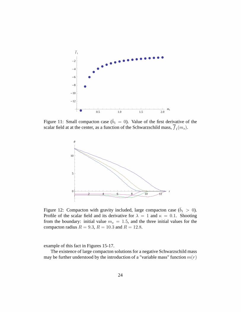
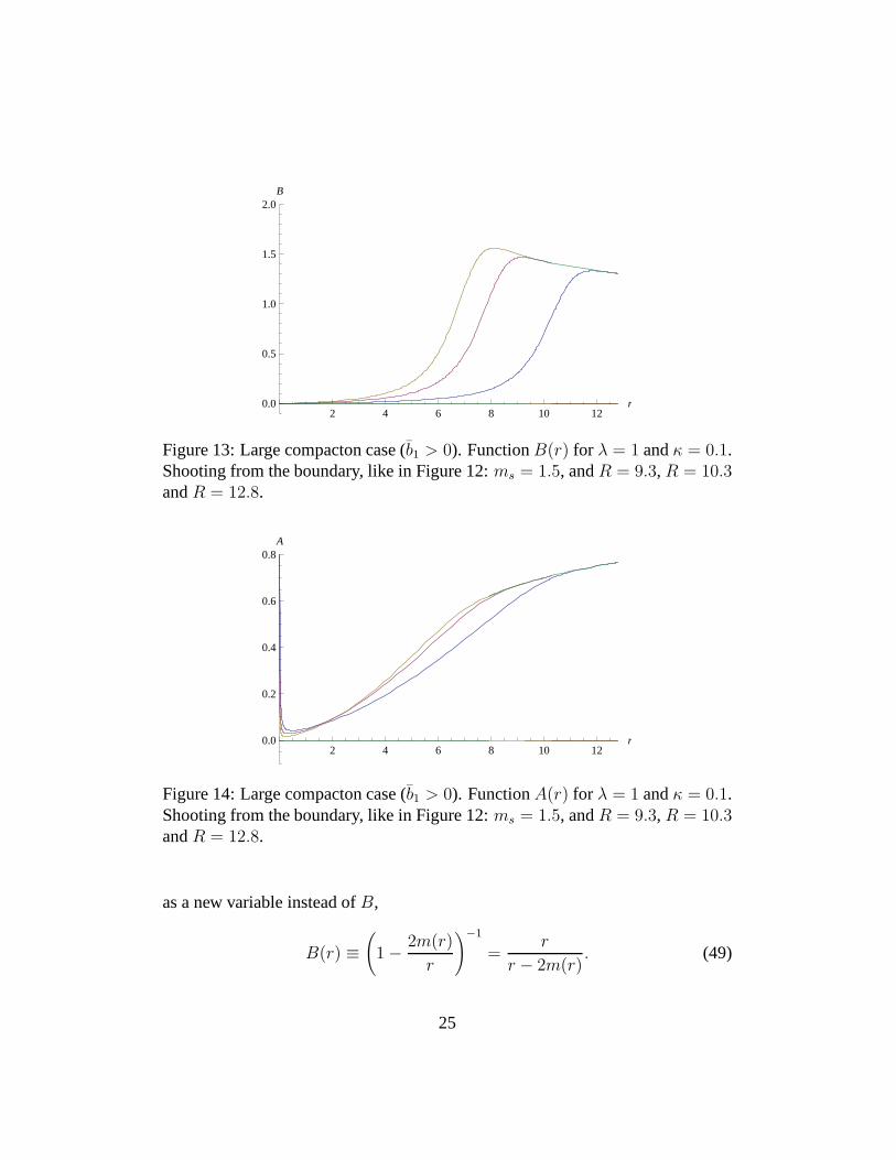
large compacton radiusR for one and the same value of the Schwarzschild mass.Some examples are shown in Figures 12-14 for the fixed valuems = 1.5 and threedifferent values of the compacton radius. It can be seen fromFigures 13, 14, thatthe functionsA andB approach the same Schwarzschild solution (with the same

20

0.5 1.0 1.5 2.0 2.5 3.0r0.0

0.2

0.4

0.6

0.8

1.0

1.2A

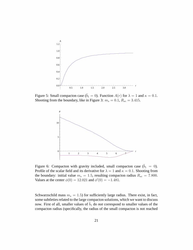
Figure 5: Small compacton case (b1 = 0). FunctionA(r) for λ = 1 andκ = 0.1.Shooting from the boundary, like in Figure 3:ms = 0.1,Rsc = 3.415.

1 2 3 4 5 6 7r0

5

10

Φ

Figure 6: Compacton with gravity included, small compactoncase (b1 = 0).Profile of the scalar field and its derivative forλ = 1 andκ = 0.1. Shooting fromthe boundary: initial valuems = 1.5, resulting compacton radiusRsc = 7.800.Values at the centerφ(0) = 12.021 andφ′(0) = −1.481.

Schwarzschild massms = 1.5) for sufficiently large radius. There exist, in fact,some subtleties related to the large compacton solutions, which we want to discussnow. First of all, smaller values ofb1 do not correspond to smaller values of thecompacton radius (specifically, the radius of the small compacton is not reached

21

1 2 3 4 5 6 7r0.0

0.5

1.0

1.5

2.0B

Figure 7: Small compacton case (b1 = 0). FunctionB(r) for λ = 1 andκ = 0.1.Shooting from the boundary, like in Figure 6:ms = 1.5,Rsc = 7.800.

1 2 3 4 5 6 7r0.0

0.2

0.4

0.6

0.8A

Figure 8: Small compacton case (b1 = 0). FunctionA(r) for λ = 1 andκ = 0.1.Shooting from the boundary, like in Figure 6:ms = 1.5,Rsc = 7.800.

by the limit b1 → 0 of the large compacton radius). Quite on the contrary, smallb1 corresponds to large compacton radius, as can be seen easilyin Figure 13. Thisdemonstrates again that the small compacton caseb1 = 0 cannot be seen as thelimiting caselim b1 → 0 of the large compacton case.

A second subtlety can be seen once we reverse the role ofms andR in the caseof the large compactons. That is to say, we choose now a fixedR and then vary

22

0.5 1.0 1.5 2.0ms

3

4

5

6

7

8

9

R

Figure 9: Small compacton case (b1 = 0). RadiusRsc of the small compacton asa function of the Schwarzschild massms.

0.5 1.0 1.5 2.0ms

4

6

8

10

12

f 0

Figure 10: Small compacton case (b1 = 0). Value of the scalar field at at thecenter, as a function of the Schwarzschild mass,f0(ms).

ms. For too largems, no solution exists. For a certain limiting value ofms, we getthe small compacton, and for even smallerms, we find the large compactons. Thequestion arises how smallms can get for a givenR such that a large compactonexists. The answer is that it can get arbitrarily small. Specifically, there existlarge compactons for negative values of the Schwarzschild massms. We show an

23

0.5 1.0 1.5 2.0ms

-12

-10

-8

-6

-4

-2

f 1

Figure 11: Small compacton case (b1 = 0). Value of the first derivative of thescalar field at at the center, as a function of the Schwarzschild mass,f 1(ms).

2 4 6 8 10 12r0

5

10

Φ

Figure 12: Compacton with gravity included, large compacton case (b1 > 0).Profile of the scalar field and its derivative forλ = 1 andκ = 0.1. Shootingfrom the boundary: initial valuems = 1.5, and the three initial values for thecompacton radiusR = 9.3,R = 10.3 andR = 12.8.

example of this fact in Figures 15-17.The existence of large compacton solutions for a negative Schwarzschild mass

may be further understood by the introduction of a "variablemass" functionm(r)

24

2 4 6 8 10 12r0.0

0.5

1.0

1.5

2.0B

Figure 13: Large compacton case (b1 > 0). FunctionB(r) for λ = 1 andκ = 0.1.Shooting from the boundary, like in Figure 12:ms = 1.5, andR = 9.3,R = 10.3andR = 12.8.

2 4 6 8 10 12r0.0

0.2

0.4

0.6

0.8A

Figure 14: Large compacton case (b1 > 0). FunctionA(r) for λ = 1 andκ = 0.1.Shooting from the boundary, like in Figure 12:ms = 1.5, andR = 9.3,R = 10.3andR = 12.8.

as a new variable instead ofB,

B(r) ≡(

1 − 2m(r)

r

)−1

=r

r − 2m(r). (49)

25

1 2 3 4 5 6r0

5

10

Φ

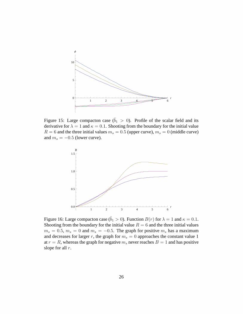
Figure 15: Large compacton case (b1 > 0). Profile of the scalar field and itsderivative forλ = 1 andκ = 0.1. Shooting from the boundary for the initial valueR = 6 and the three initial valuesms = 0.5 (upper curve),ms = 0 (middle curve)andms = −0.5 (lower curve).

1 2 3 4 5 6r0.0

0.5

1.0

1.5B

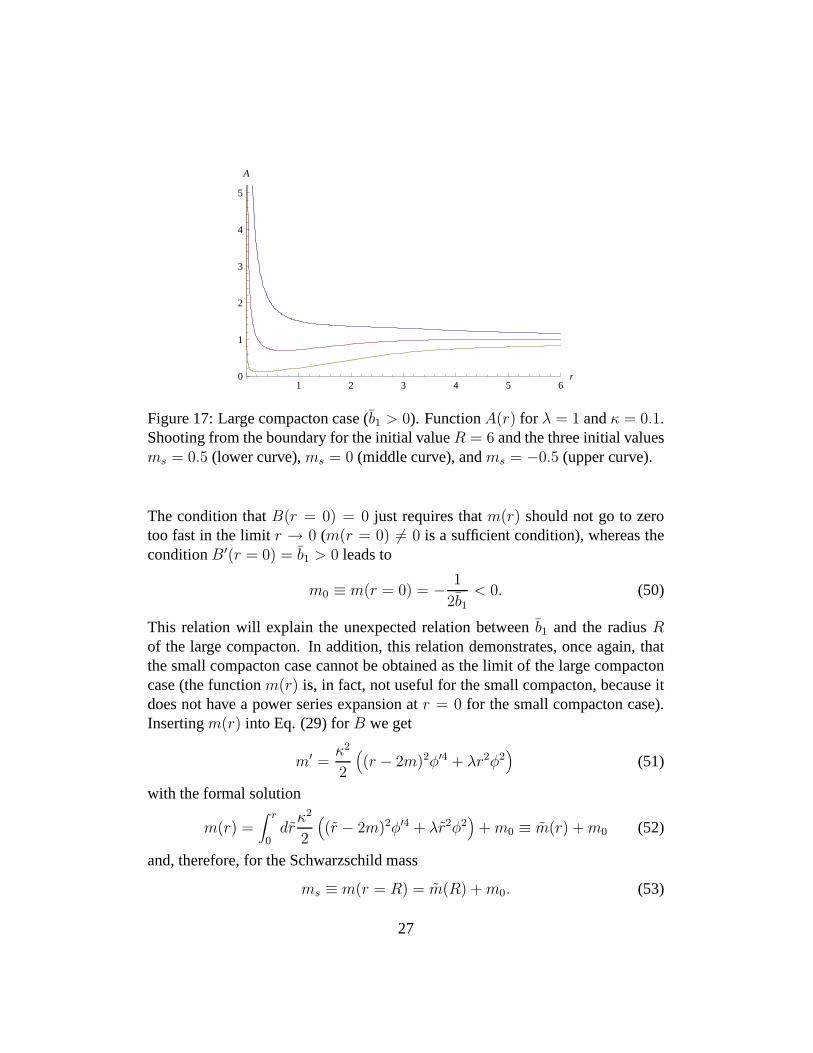
Figure 16: Large compacton case (b1 > 0). FunctionB(r) for λ = 1 andκ = 0.1.Shooting from the boundary for the initial valueR = 6 and the three initial valuesms = 0.5, ms = 0 andms = −0.5. The graph for positivems has a maximumand decreases for largerr, the graph forms = 0 approaches the constant value 1atr = R, whereas the graph for negativems never reachesB = 1 and has positiveslope for allr.

26

1 2 3 4 5 6r0

1

2

3

4

5

A

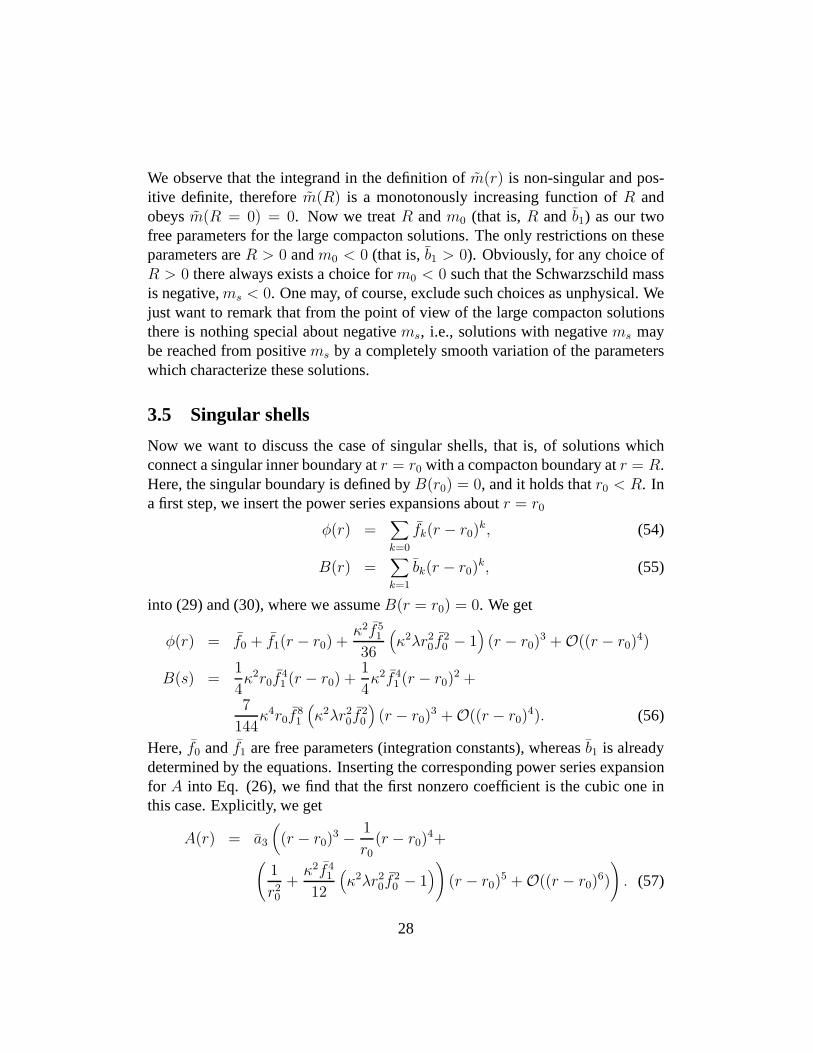
Figure 17: Large compacton case (b1 > 0). FunctionA(r) for λ = 1 andκ = 0.1.Shooting from the boundary for the initial valueR = 6 and the three initial valuesms = 0.5 (lower curve),ms = 0 (middle curve), andms = −0.5 (upper curve).

The condition thatB(r = 0) = 0 just requires thatm(r) should not go to zerotoo fast in the limitr → 0 (m(r = 0) 6= 0 is a sufficient condition), whereas theconditionB′(r = 0) = b1 > 0 leads to

m0 ≡ m(r = 0) = − 1

2b1< 0. (50)

This relation will explain the unexpected relation betweenb1 and the radiusRof the large compacton. In addition, this relation demonstrates, once again, thatthe small compacton case cannot be obtained as the limit of the large compactoncase (the functionm(r) is, in fact, not useful for the small compacton, because itdoes not have a power series expansion atr = 0 for the small compacton case).Insertingm(r) into Eq. (29) forB we get

m′ =κ2

2

(

(r − 2m)2φ′4 + λr2φ2)

(51)

with the formal solution

m(r) =∫ r

0drκ2

2

(

(r − 2m)2φ′4 + λr2φ2)

+m0 ≡ m(r) +m0 (52)

and, therefore, for the Schwarzschild mass

ms ≡ m(r = R) = m(R) +m0. (53)

27

We observe that the integrand in the definition ofm(r) is non-singular and pos-itive definite, thereforem(R) is a monotonously increasing function ofR andobeysm(R = 0) = 0. Now we treatR andm0 (that is,R and b1) as our twofree parameters for the large compacton solutions. The onlyrestrictions on theseparameters areR > 0 andm0 < 0 (that is,b1 > 0). Obviously, for any choice ofR > 0 there always exists a choice form0 < 0 such that the Schwarzschild massis negative,ms < 0. One may, of course, exclude such choices as unphysical. Wejust want to remark that from the point of view of the large compacton solutionsthere is nothing special about negativems, i.e., solutions with negativems maybe reached from positivems by a completely smooth variation of the parameterswhich characterize these solutions.

3.5 Singular shells

Now we want to discuss the case of singular shells, that is, ofsolutions whichconnect a singular inner boundary atr = r0 with a compacton boundary atr = R.Here, the singular boundary is defined byB(r0) = 0, and it holds thatr0 < R. Ina first step, we insert the power series expansions aboutr = r0

φ(r) =∑

k=0

fk(r − r0)k, (54)

B(r) =∑

k=1

bk(r − r0)k, (55)

into (29) and (30), where we assumeB(r = r0) = 0. We get

φ(r) = f0 + f1(r − r0) +κ2f 5

1

36

(

κ2λr20f

20 − 1

)

(r − r0)3 + O((r − r0)

4)

B(s) =1

4κ2r0f

41 (r − r0) +

1

4κ2f 4

1 (r − r0)2 +

7

144κ4r0f

81

(

κ2λr20f

20

)

(r − r0)3 + O((r − r0)

4). (56)

Here,f0 andf1 are free parameters (integration constants), whereasb1 is alreadydetermined by the equations. Inserting the corresponding power series expansionfor A into Eq. (26), we find that the first nonzero coefficient is the cubic one inthis case. Explicitly, we get

A(r) = a3

(

(r − r0)3 − 1

r0(r − r0)

4+(

1

r20

+κ2f 4

1

12

(

κ2λr20f

20 − 1

)

)

(r − r0)5 + O((r − r0)

6)

)

. (57)

28

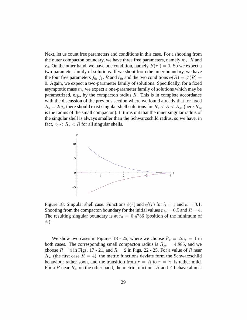
Next, let us count free parameters and conditions in this case. For a shooting fromthe outer compacton boundary, we have three free parameters, namelyms, R andr0. On the other hand, we have one condition, namelyB(r0) = 0. So we expect atwo-parameter family of solutions. If we shoot from the inner boundary, we havethe four free parametersf0, f1,R andr0, and the two conditionsφ(R) = φ′(R) =0. Again, we expect a two-parameter family of solutions. Specifically, for a fixedasymptotic massms we expect a one-parameter family of solutions which may beparametrized, e.g., by the compacton radiusR. This is in complete accordancewith the discussion of the previous section where we found already that for fixedRs ≡ 2ms there should exist singular shell solutions forRs < R < Rsc (hereRsc

is the radius of the small compacton). It turns out that the inner singular radius ofthe singular shell is always smaller than the Schwarzschildradius, so we have, infact,r0 < Rs < R for all singular shells.

1 2 3 4r

-5

0

5

10

Φ

Figure 18: Singular shell case. Functionsφ(r) andφ′(r) for λ = 1 andκ = 0.1.Shooting from the compacton boundary for the initial valuesms = 0.5 andR = 4.The resulting singular boundary is atr0 = 0.4736 (position of the minimum ofφ′).

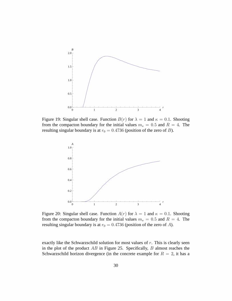
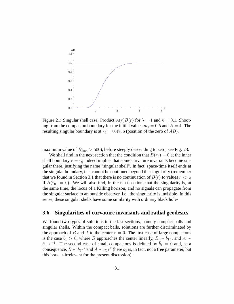
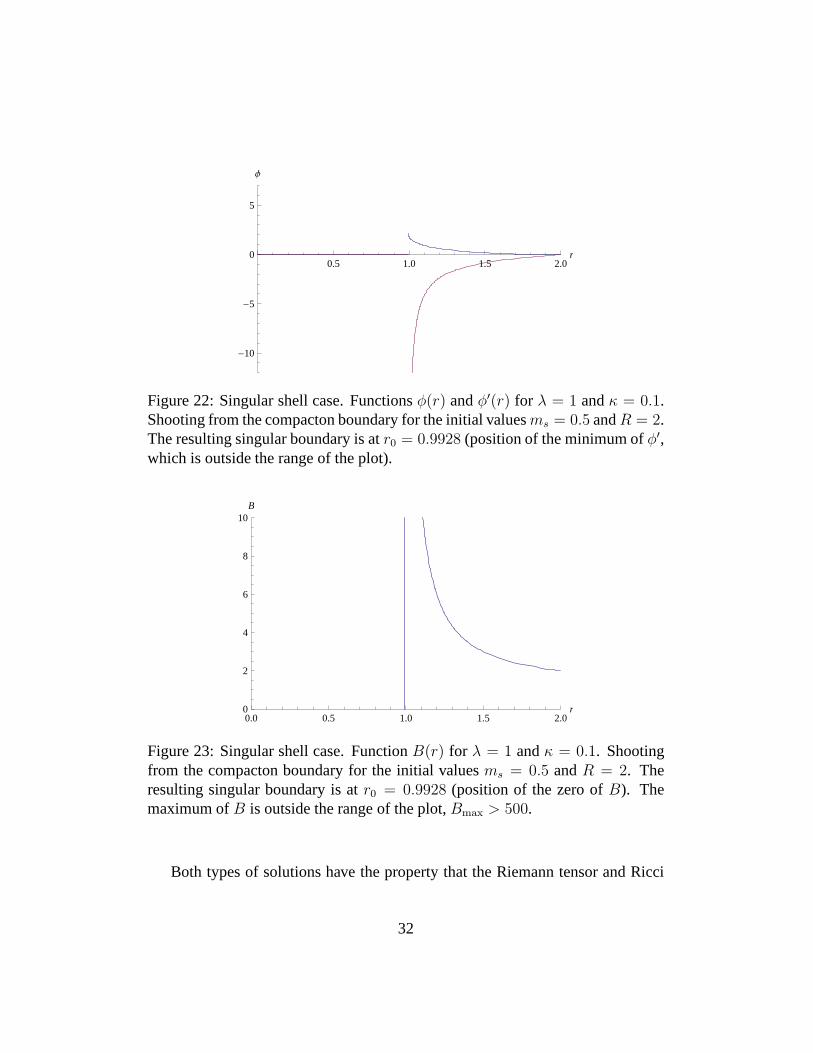
We show two cases in Figures 18 - 25, where we chooseRs ≡ 2ms = 1 inboth cases. The corresponding small compacton radius isRsc = 4.885, and wechooseR = 4 in Figs. 17 - 21, andR = 2 in Figs. 22 - 25. For a value ofR nearRsc (the first caseR = 4), the metric functions deviate form the Schwarzschildbehaviour rather soon, and the transition fromr = R to r = r0 is rather mild.For aR nearRs, on the other hand, the metric functionsB andA behave almost

29

0 1 2 3 4r0.0

0.5

1.0

1.5

2.0B

Figure 19: Singular shell case. FunctionB(r) for λ = 1 andκ = 0.1. Shootingfrom the compacton boundary for the initial valuesms = 0.5 andR = 4. Theresulting singular boundary is atr0 = 0.4736 (position of the zero ofB).

0 1 2 3 4r0.0

0.2

0.4

0.6

0.8

1.0A

Figure 20: Singular shell case. FunctionA(r) for λ = 1 andκ = 0.1. Shootingfrom the compacton boundary for the initial valuesms = 0.5 andR = 4. Theresulting singular boundary is atr0 = 0.4736 (position of the zero ofA).

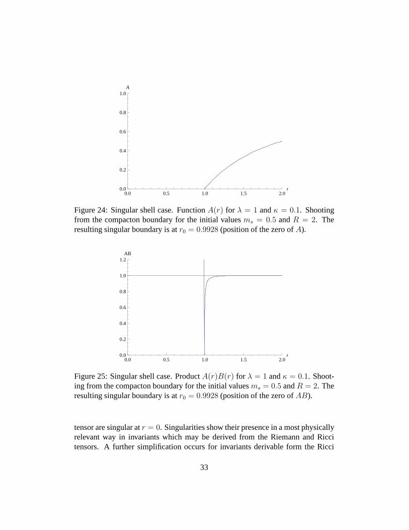
exactly like the Schwarzschild solution for most values ofr. This is clearly seenin the plot of the productAB in Figure 25. Specifically,B almost reaches theSchwarzschild horizon divergence (in the concrete examplefor R = 2, it has a

30

1 2 3 4r0.0

0.2

0.4

0.6

0.8

1.0

1.2AB

Figure 21: Singular shell case. ProductA(r)B(r) for λ = 1 andκ = 0.1. Shoot-ing from the compacton boundary for the initial valuesms = 0.5 andR = 4. Theresulting singular boundary is atr0 = 0.4736 (position of the zero ofAB).

maximum value ofBmax > 500), before steeply descending to zero, see Fig. 23.We shall find in the next section that the condition thatB(r0) = 0 at the inner

shell boundaryr = r0 indeed implies that some curvature invariants become sin-gular there, justifying the name "singular shell". In fact,space-time itself ends atthe singular boundary, i.e., cannot be continued beyond thesingularity (rememberthat we found in Section 3.1 that there is no continuation ofB(r) to valuesr < r0if B(r0) = 0). We will also find, in the next section, that the singularityis, atthe same time, the locus of a Killing horizon, and no signals can propagate fromthe singular surface to an outside observer, i.e., the singularity is invisible. In thissense, these singular shells have some similarity with ordinary black holes.

3.6 Singularities of curvature invariants and radial geodesics

We found two types of solutions in the last sections, namely compact balls andsingular shells. Within the compact balls, solutions are further discriminated bythe approach ofB andA to the centerr = 0. The first case of large compactonsis the caseb1 > 0, whereB approaches the center linearly,B ∼ b1r, andA ∼a−1r

−1. The second case of small compactons is defined byb1 = 0 and, as aconsequence,B ∼ b2r

2 andA ∼ a2r2 (hereb2 is, in fact, not a free parameter, but

this issue is irrelevant for the present discussion).

31

0.5 1.0 1.5 2.0r

-10

-5

0

5

Φ

Figure 22: Singular shell case. Functionsφ(r) andφ′(r) for λ = 1 andκ = 0.1.Shooting from the compacton boundary for the initial valuesms = 0.5 andR = 2.The resulting singular boundary is atr0 = 0.9928 (position of the minimum ofφ′,which is outside the range of the plot).

0.0 0.5 1.0 1.5 2.0r0

2

4

6

8

10B

Figure 23: Singular shell case. FunctionB(r) for λ = 1 andκ = 0.1. Shootingfrom the compacton boundary for the initial valuesms = 0.5 andR = 2. Theresulting singular boundary is atr0 = 0.9928 (position of the zero ofB). Themaximum ofB is outside the range of the plot,Bmax > 500.

Both types of solutions have the property that the Riemann tensor and Ricci

32

0.0 0.5 1.0 1.5 2.0r0.0

0.2

0.4

0.6

0.8

1.0A

Figure 24: Singular shell case. FunctionA(r) for λ = 1 andκ = 0.1. Shootingfrom the compacton boundary for the initial valuesms = 0.5 andR = 2. Theresulting singular boundary is atr0 = 0.9928 (position of the zero ofA).

0.0 0.5 1.0 1.5 2.0r0.0

0.2

0.4

0.6

0.8

1.0

1.2AB

Figure 25: Singular shell case. ProductA(r)B(r) for λ = 1 andκ = 0.1. Shoot-ing from the compacton boundary for the initial valuesms = 0.5 andR = 2. Theresulting singular boundary is atr0 = 0.9928 (position of the zero ofAB).

tensor are singular atr = 0. Singularities show their presence in a most physicallyrelevant way in invariants which may be derived from the Riemann and Riccitensors. A further simplification occurs for invariants derivable form the Ricci

33

tensor alone, because then the Einstein equations may be used. Concretely wefind for the Ricci scalar

R = −κ2T µµ = 4κ2λφ2 (58)

so the Ricci scalar is, in fact, regular at the origin or the singular boundary, becausethe scalar fieldφ is. The Ricci tensor squared may be expressed like

RµνRµν = κ4(

TµνTµν + (T µ

µ )2)

= κ4

(

3

4

φ′8

B4+ 20λ2φ4

)

(59)

where we used

TµνTµν =

3

4

φ′8

B4+ 4λ2φ4. (60)

Here, the first term is singular atr = 0, becauseφ′ is regular and non-zero therewhereasB goes to zero liker (large compacton),r2 (small compacton), or(r −r0) (singular shell), respectively. Therefore, the Ricci tensor squared is alreadysingular. More complicated invariants like, e.g., the Kretschmann invariant, aresingular, as well.

One possible question to be asked in connection with these singularities iswhether they really belong to the space time manifold, that is, whether a freelyfalling particle may reach them in finite proper time. We willfind in all threecases that this is the case, i.e. there exist geodesics whichhit the singularities infinite proper time. For this purpose we have to study the geodesic equation

xµ(τ) + Γµαβ x

αxβ = 0. (61)

HereΓµαβ is the Christoffel connection andτ is the proper time. We shall restrict

to radial geodesics, which is sufficient for our purpose. In this case the geodesicequations reduce to

t+ Γtttt

2 + 2Γttr tr + Γt

rrr2 = 0

r + Γrttt

2 + 2Γrtr tr + Γr

rrr2 = 0 (62)

where the nonzero components of the Christoffel connectionare

Γttr =

1

2gtt∂rgtt =

1

2

A′

A

Γrtt = −1

2grr∂rgtt =

1

2

A′

B

Γrrr =

1

2grr∂rgrr =

1

2

B′

B(63)

34

We are interested in the geodesic motion near the singularity, therefore it is enoughfor our purposes to restrict to the leading behaviour ofA andB. In the largecompacton case , this leading behaviour isA ∼ (a−1/r) andB ∼ b1r and we getthe geodesic equations

t− 1

rtr = 0

r − γ

2r3t2 +

1

2rr2 = 0 (64)

whereγ ≡ (a−1/b1). The equation fort has the solution

t = c1

∫ τ

τ0dτ ′r(τ ′) + c2 (65)

and the equation forr becomes

r − c3r

+1

2rr2 = 0 (66)

wherec3 ≡ (γc21/2) > 0. Under the transformationr = f2

3 the last equation turnsinto

f =3c32f− 1

3 . (67)

This last equation has an easy interpretation in terms of an equivalent mechanicalsystem. It is just the e.o.m. of a nonrelativistic particle in one dimension in therepulsive external potentialU(f) ∼ −f 2

3 . The centerf = 0 of the potential maybe reached despite its repulsive nature because of the positive power(2/3) in thedistance law. However, not all radial geodesics hit the center r = 0, because inthe equivalent mechanical problem the particle needs a sufficient initial velocity.

The small compacton case may be analysed in an equivalent manner. Theleading behaviour isA ∼ a2r

2 andB ∼ b2r2 and we get the geodesic equations

t+2

rtr = 0

r +γ

rt2 +

1

rr2 = 0 (68)

whereγ ≡ (a2/b2). The equation fort has the solution

t = c1

∫ τ

τ0

dτ ′

r2(τ ′)+ c2 (69)

35

and the equation forr becomes

r +c3r5

+1

rr2 = 0 (70)

wherec3 ≡ (γc21/2) > 0. Under the transformationr = f1

2 the last equation turnsinto

f = −2c3f 2. (71)

This is the e.o.m. of a nonrelativistic one-dimensional particle in an attractive1/fpotential. The particle will hit the centerf = 0 unless it has a sufficiently large(outward directed) initial escape velocity.

Finally, for the singular shell it is useful to introduce thevariableu = r − r0.Then the leading behaviour isA ∼ a3u

3 andB ∼ b1u and we get the geodesicequations

t+3

utu = 0

u+3γu

2t2 +

1

2uu2 = 0 (72)

whereγ ≡ (a3/b1). The equation fort has the solution

t = c1

∫ τ

τ0

dτ ′

u3(τ ′)+ c2 (73)

and the equation foru becomes

u+c3u5

+1

2uu2 = 0 (74)

wherec3 ≡ (3γc21/2) > 0. Under the transformationu = f2

3 the last equationturns into

f = − 3c32f 3

. (75)

This is the e.o.m. of a nonrelativistic one-dimensional particle in an attractive1/f 2 potential. The particle will hit the centerf = 0 unless it has a sufficientlylarge (outward directed) initial escape velocity.

We conclude that in all cases there exist radial geodesics which hit the singu-larities atr = 0 or r = r0, respectively, therefore these singularities belong to thecorresponding space time manifolds.

36

The singular shells, however, differ from the compact ballsin one essentialaspect, in that their singular inner boundary is, at the sametime, the locus of aKilling horizon and, therefore, invisible for an outside observer. In a first step, letus consider the equation for a light-like radial geodesic. We find

ds2 = 0 = −Adt2 +Bdr2 ⇒ dt =

√

B

Adr (76)

and withB/A ∼ (c/(r − r0))2 nearr = r0 we find the solution

r(t) − r0 = exp(

t− t0c

)

(77)

wheret0 is an integration constant. Obviously,r = r0 requirest = −∞, so alight ray cannot escape from the singular surface. A slightly more rigorous andless coordinate dependent derivation uses the concept of a Killing horizon. Let usassume the existence of a Killing vectorξ and consider the set of points (hyper-surface)H0 whereξ is null, i.e.,N ≡ (ξ, ξ) = 0. A Killing horizon H is aconnected componentH ∈ H0 which is, at the same time, a null hyper-surface,i.e.,M ≡ (dN, dN) = 0. So let us demonstrate that the inner boundary of thesingular shell is indeed a Killing horizon. For the Killing vector we choose thegenerator of time translationsξ = (∂/∂t) ≡ ∂t, as is obvious for a static space-time. ForN we find

N ≡ (ξ, ξ) = gµνdxµ ⊗ dxν(∂t, ∂t) = −A. (78)

As nearr = r0 A behaves likeA ∼ a3(r − r0)3, it holds thatN(r0) = 0. ForM

we get withdN = −A′dr

M ≡ (dN, dN) = A′2gµν∂µ ⊗ ∂ν(dr, dr) =A′2

B. (79)

With the leading behaviour ofA nearr0 like above andB ∼ b1(r − r0), weeasily conclude that indeedM(r0) = 0, so the singular boundary is a Killinghorizon. We remind the reader that for static space-times every event horizon isa Killing horizon, which makes our result all the more interesting. The singularshell solutions we found are, in fact, quite similar to ordinary black holes in thisrespect.

37

4 Discussion

It has been the main purpose of the present article to investigate in detail the prop-erties of compact boson stars (compact balls or shells minimally coupled to grav-ity) for a theory with a non-standard kinetic term in three plus one dimensions.We chose the simplest possible theory for this purpose, witha purely quartic ki-netic term and the simple quadratic potential, because we wanted to pursue theanalytical investigation as far as possible in order to understand also more genericand qualitative features, in addition to explicit numerical calculations. This theoryhas a one-parameter family of compact ball solutions already in the case withoutgravity. The compact balls in the theory without gravity turn out to be solutionsof the weak type, which solve the field equations everywhere except at the ori-gin. We remark that this fact is not a problem in the case at hand, because theset of weak solutions is the appropriate solution set for variational problems ofthis type, in any case. Alternatively, the compact ball solutions may be extendedto solutions in the whole space by introducing a delta function source term at theorigin. It turned out that these solutions may have arbitrary size and energy.

In the case with gravity, we found two different types of solutions, both ofwhich are of the strong type, i.e., they solve the field equations everywhere. Forcompact balls, we found that the scalar field itself is behaving well at the origin(it has a power series expansion there). The metric coefficients do have a powerseries expansion at the origin, as well, (with the exceptionof ar−1 leading term inone specific case), but nevertheless give rise to a singularity atr = 0. Specifically,some higher invariants of the Riemann tensor, like the Riccitensor squared, orthe Kretschmann invariant, become singular at this point. This singularity is notshielded by any horizon, so it is a naked singularity. In spite of the naked sin-gularity at the center, asymptotically these solutions behave like Schwarzschildsolutions, so they have finite Schwarzschild mass (or asymptotic, ADM mass)ms. In one class of solutions (the large compactons), this ADM mass may takeon negative values, in spite of the positive definite energy density. The theoremsexcluding this type of behaviour are evaded by the presence of naked singularitiesin the case at hand.

In addition, we found another type of solutions in the theorywith gravity,namely the singular shells where a singularity already forms at a finite, nonzerovalue of the radial coordinate. This singularity is a surface in space with finitearea, as may be checked easily by inspecting the corresponding metric (the angu-lar part of the metric is not multiplied by any suppressing factor at the positionr = r0 of the singularity). Further, this singularity is a genuinesingular boundary

38

of space-time, because space-time cannot be continued beyond this boundary. Atthe same time, this singular boundary is a Killing horizon. In addition, the sin-gular shells asymptotically for large radius are Schwarzschild, so they resembleordinary Schwarzschild black holes in many respects. Certainly they are black(i.e., no radiation may escape from the horizon), although the curvature near thehorizon is different from the Schwarzschild black hole case. It is probably morea question of parlance whether these objects should be called genuine black holes- thereby providing a counter-example to the scalar no hair conjecture - or inter-preted as different object which, nevertheless, share manyproperties with ordinaryblack holes. In any case, the existence of these singular shell solutions is interest-ing. On the other hand, ordinary Schwarzschild black hole solutions (where thecurvature near the horizon behaves like in the Schwarzschild case) do not exist inour model, except for the trivial case where the metric is exactly Schwarzschildeverywhere and the scalar field takes its vacuum value in all space-time.

At this point, an obvious question to ask is whether theoriesof the type pre-sented here may be of some relevance in astrophysical or cosmological contexts.The theory presented here is the simplest possible case of the class of theorieshaving a non-standard kinetic term and allowing for compactboson stars. There-fore, an attempt for direct applications would most likely be premature, and weshall focus, instead, on more generic issues. Specifically,we want to commenton some features of these theories which might make them interesting for as-trophysical considerations. A first feature we already mentioned is the fact thatnon-overlapping multi compact ball configurations do not interact at all in thecase without gravity, so the self-gravitating ones only interact via the universalgravitational interaction. A further feature of compact solitons in K field theoriesin general is the fact that linear fluctuations are possible only inside the compactsolitons, whereas they are completely suppressed in the vacuum. This fact is easyto understand. Unlike for the standard kinetic term, in the case of a non-standardK theory the wave operator acting on the fluctuation fieldδφ is multiplied by somepower ofX ≡ ∂µφ∂µφ, whereX has to be evaluated at the background field (i.e.,the compacton). ButX is identically zero outside the compacton (that is, in theregion where the background field takes its vacuum value), which is the reason forthe complete suppression of linear fluctuations in that region. This implies that acompacton in K field theories cannot emit particle type radiation, which makes it arather stable object. These two facts - that compact boson stars only interact grav-itationally, and that particle-like excitations in vacuumdo not exist - might makecompact boson stars of the type discussed in this paper interesting candidates fordark matter. The second fact may, further, give rise to the following speculations.

39

Let us assume for a moment that a universe with a scalar K field theory was areasonably good effective description in a certain (early)stage of the evolution ofthe universe. Then linear fluctuations of the K field which mayact as seeds formatter formation were naturally present in the compacton regions, but absent inthe vacuum regions. The late time remnants of the former would be regions of theuniverse with a higher matter concentration, whereas the latter might have evolvedinto voids (low matter density regions).

Before more convincing conclusions can be drawn with respect to possibleapplications of compact boson stars, one key issue to understand is which featuresof the theory presented in this article are generic and whichare just artifacts of thespecific model. One important feature in this respect obviously is the presence ofnaked singularities in the compact ball type solutions of the model studied in thispaper. Such naked singularities of the point-like type are already present in finitemass solutions (boson stars) for standard self-gravitating scalar fields [29] - [32].Further, it is known that the gravitational collapse of a standard scalar field mayterminate in a naked singularity [39], [40]. Nevertheless,the presence of nakedsingularities is frequently viewed as an unwanted or even unphysical feature and,in any case, the generic or non-generic nature of naked singularities in compactballs is an interesting question. We cannot give a completely mathematically rig-orous answer to this question, but shall try to partially answer it relying on ourexperience and some recent results in the literature. On theone hand, for a static,radially symmetric scalar field, it seems to be a typical feature that non-singularmetric functionsA, B at the originr = 0 require that the scalar field takes itsvacuum value there. Further, these local solutions typically are isolated solutions(i.e., without free integration constants) which makes it difficult to connect themto finite mass (i.e., Schwarzschild) asymptotic solutions.In our specific model,we could exclude this possibility, whereas in more general theories it might stillbe possible to connect a regular center with an asymptotic Schwarzschild solutionprovided thati) the scalar field has more than one vacuum andii) the scalar fieldLagrangian contains sufficiently many coupling constants which may be varied inorder to connect the two local solutions near zero and near infinity.

There exists, however, a class of slightly different but related theories wherethe appearance of compact balls with a regular center seems to be a more genericfeature, namely the class of self-gravitating compact Q balls. A Q ball is a com-plex scalar fieldψ restricted to the ansatzψ = exp(iωt)φ(~x), such that the re-sulting static equations for the real functionφ are quite similar to the static fieldequations of a real scalar field, both with and without gravitation. Q balls (withoutgravitation) were introduced by S. Coleman in [41] and have been widely inves-

40

tigated since then. Systems of self-gravitating Q balls arefrequently subsumedunder the general notion of boson stars. For more details we refer to the reviewarticles [36] - [38]. Compact Q balls (without gravity) for acomplex scalar the-ory with a standard kinetic term but with a V-shaped potential have recently beenfound in [6] and in [7] (the second paper included also an electromagnetic inter-action of the complex scalar, and allows both for ball-shaped and shell-shapedsolutions). The gravitational counterpart of the model studied in [7] was investi-gated in [28], mainly using numerical methods, and the existence of non-singularsolutions (both of the ball type and of the shell type) was established. Therefore,the existence of regular self-gravitating compact solutions seems to be a moregeneric feature for Q balls, analogously to the case of standard (non-compact) Qballs.

In any case, we think that the further study of the interaction between compactobjects (like compact solitons, Q balls, etc.) and gravitation is an interesting en-deavour which may lead to new insights and unexpected phenomena, as well assome applications to astrophysics and cosmology. One future line of investigationwill certainly be the study of Q balls. Another promising direction is the analysisof the symmetries and conservation laws of the corresponding theories, e.g., alongthe lines of [42] - [45], which may lead to a better understanding of more generalsolutions as well as their stability. These issues are undercurrent investigation.

Acknowledgements

C.A., P.K. and J.S.-G. thank MCyT (Spain) and FEDER (FPA2005-01963), andsupport from Xunta de Galicia (grant PGIDIT06PXIB296182PRand Conselleriade Educacion). A.W. acknowledges support from the Foundation for Polish Sci-ence FNP (KOLUMB programme 2008/2009) and Ministry of Science and HigherEducation of Poland grant N N202 126735 (2008-2010). N.E.G.is partially sup-ported by the ANPCyT Grant PICT-2007-00849. He was visitingICTP under theICTP associate program during the late stages of this work, and wants to thankthe ICTP for providing support and an extremely comfortablework environment.

References

[1] H. Arodz, Acta Phys. Polon. B33 (2002) 1241 [arXiv:nlin/0201001].

41

[2] H. Arodz, P. Klimas and T. Tyranowski, Acta Phys. Polon. B36 (2005) 3861[arXiv:hep-th/0510204].

[3] H. Arodz, P. Klimas and T. Tyranowski, Phys. Rev. E73 (2006) 046609[arXiv:hep-th/0511022].

[4] H. Arodz, P. Klimas and T. Tyranowski, Acta Phys. Polon. B38 (2007) 3099[arXiv:hep-th/0701148].

[5] H. Arodz, P. Klimas and T. Tyranowski, Phys. Rev. D77 (2008) 047701[arXiv:0710.2244 [hep-th]].

[6] H. Arodz and J. Lis, Phys. Rev. D77 (2008) 107702 [arXiv:0803.1566 [hep-th]].

[7] H. Arodz and J. Lis, Phys. Rev. D79 (2009) 045002 [arXiv:0812.3284 [hep-th]].

[8] H. Arodz, J. Karkowski and Z. Swierczynski, arXiv:0907.2801 [hep-th].

[9] Gaeta G, Gramchev T and Walcher S 2007 J. Phys. A404493

[10] Kuru S, arXiv:0811.0706

[11] C. Adam, J. Sanchez-Guillen and A. Wereszczynski, J. Phys. A 40 (2007)13625 [Erratum-ibid. A42 (2009) 089801] [arXiv:0705.3554 [hep-th]].

[12] D. Bazeia, L. Losano and R. Menezes, Phys. Lett. B668 (2008) 246[arXiv:0807.0213 [hep-th]].

[13] C. Armendariz-Picon, T. Damour and V. F. Mukhanov, Phys. Lett. B 458(1999) 209 [arXiv:hep-th/9904075].

[14] T. Chiba, T. Okabe and M. Yamaguchi, Phys. Rev. D62 (2000) 023511[arXiv:astro-ph/9912463].

[15] C. Armendariz-Picon, V. F. Mukhanov and P. J. Steinhardt, Phys. Rev. Lett.85 (2000) 4438 [arXiv:astro-ph/0004134].

[16] C. Armendariz-Picon, V. F. Mukhanov and P. J. Steinhardt, Phys. Rev. D63(2001) 103510 [arXiv:astro-ph/0006373].

[17] R. J. Scherrer, Phys. Rev. Lett.93 (2004) 011301 [arXiv:astro-ph/0402316].

42

[18] L. P. Chimento and A. Feinstein, Mod. Phys. Lett. A19 (2004) 761[arXiv:astro-ph/0305007].

[19] E. Babichev, Phys. Rev. D74 (2006) 085004 [arXiv:hep-th/0608071].

[20] E. Babichev, Phys. Rev. D77 (2008) 065021 [arXiv:0711.0376 [hep-th]].

[21] P. Rosenau and J. M. Hyman, Phys. Rev. Lett.70 (1993) 564.

[22] F. Cooper, H. Shepard and P. Sodano, Phys. Rev. E48 (1993) 4027.

[23] C. Adam, P. Klimas, J. Sanchez-Guillen and A. Wereszczynski, J. Phys. A42 (2009) 135401 [arXiv:0811.4503 [hep-th]].

[24] C. Adam, P. Klimas, J. Sanchez-Guillen and A. Wereszczynski,arXiv:0902.0880 [hep-th].

[25] C. Adam, N. Grandi, J. Sanchez-Guillen and A. Wereszczynski, J. Phys.A 41 (2008) 212004 [Erratum-ibid. A42 (2009) 159801] [arXiv:0711.3550[hep-th]].

[26] C. Adam, N. Grandi, P. Klimas, J. Sanchez-Guillen and A.Wereszczynski,J. Phys. A41 (2008) 375401 [arXiv:0805.3278 [hep-th]].

[27] D. Bazeia, A. R. Gomes, L. Losano and R. Menezes, Phys. Lett. B 671(2009) 402 [arXiv:0808.1815 [hep-th]].

[28] B. Kleihaus, J. Kunz, C. Lammerzahl and M. List, arXiv:0902.4799 [gr-qc].

[29] H. A. Buchdahl, Phys. Rev.115(1959) 1325.

[30] M. Wyman, Phys. Rev. D24 (1981) 839.

[31] A. G. Agnese and M. La Camera, Phys. Rev. D31 (1985) 1280.

[32] B. C. Xanthopoulos and T. Zannias, Phys. Rev. D40 (1989) 2564.

[33] D. J. Kaup, Phys. Rev.172(1968) 1331.

[34] R. Ruffini and S. Bonazzola, Phys. Rev.187(1969) 1767.

[35] M. Gleiser, Phys. Rev. D38 (1988) 2376 [Erratum-ibid. D39 (1989) 1258].

[36] P. Jetzer, Phys. Rept.220(1992) 163.

43

[37] T. D. Lee and Y. Pang, Phys. Rept.221(1992) 251.

[38] F. E. Schunck and E. W. Mielke, Class. Quant. Grav.20 (2003) R301[arXiv:0801.0307 [astro-ph]].

[39] D. Christodoulou, Annals Math.140(1994) 607.

[40] I. H. Dwivedi and P. S. Joshi, Commun. Math. Phys.166 (1994) 117[arXiv:gr-qc/9405049].

[41] S. R. Coleman, Nucl. Phys. B262 (1985) 263 [Erratum-ibid. B269 (1986)744].

[42] O. Alvarez, L. A. Ferreira and J. Sanchez Guillen, Nucl.Phys. B529(1998)689 [arXiv:hep-th/9710147].

[43] O. Alvarez, L. A. Ferreira and J. Sanchez-Guillen, Int.J. Mod. Phys. A24(2009) 1825 [arXiv:0901.1654 [hep-th]].

[44] C. Adam and J. Sanchez-Guillen, JHEP0501 (2005) 004[arXiv:hep-th/0412028].

[45] C. Adam, J. Sanchez-Guillen and A. Wereszczynski, J. Math. Phys.48(2007) 032302 [arXiv:hep-th/0610227].

44