COMP60611 Fundamentals of Parallel and Distributed Systems

Combining the strengths of UMIST andThe Victoria University of Manchester

COMP60611 Fundamentals of Paralleland Distributed Systems

Lecture 7

Scalability Analysis

John Gurd, Graham Riley

Centre for Novel Computing

School of Computer Science

University of Manchester

October 2010 2

Scalability

• What do we mean by scalability?

– Scalability applies to an algorithm executing on a parallel computer, not simply to an algorithm!

• How does an algorithm behave for a fixed problem size as the number of processors used increases?

– This is known as strong scaling.

• How does an algorithm behave as the problem size changes, in addition to changing the number of processors?

• A key insight is to look at how efficiency changes.

October 2010 3

Efficiency and Strong Scaling• Typically, for a fixed problem size, N, the efficiency

of an algorithm decreases as P increases. (Why?)

– Overheads typically do not get smaller as P increases. They remain ‘fixed’ or, worse, they may grow with P (e.g. the number of communications may grow – in an all-to-all communication pattern).

• Recall that:

refabs

ref

1.

1 PP

TE

POPTT

October 2010 4

Efficiency and Strong Scaling

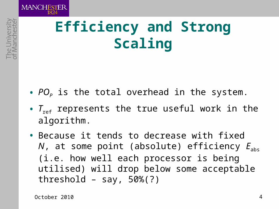
• POP is the total overhead in the system.

• Tref represents the true useful work in the algorithm.

• Because it tends to decrease with fixed N, at some point (absolute) efficiency Eabs (i.e. how well each processor is being utilised) will drop below some acceptable threshold – say, 50%(?)

October 2010 5

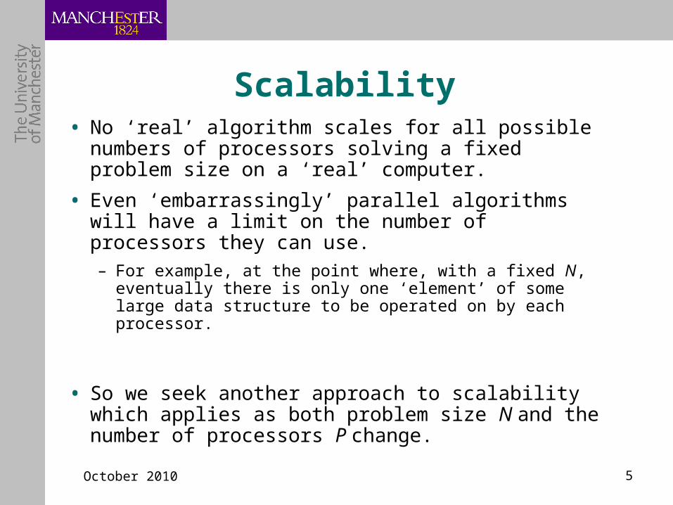
Scalability• No ‘real’ algorithm scales for all possible numbers

of processors solving a fixed problem size on a ‘real’ computer.

• Even ‘embarrassingly’ parallel algorithms will have a limit on the number of processors they can use.– For example, at the point where, with a fixed N, eventually

there is only one ‘element’ of some large data structure to be operated on by each processor.

• So we seek another approach to scalability which applies as both problem size N and the number of processors P change.

October 2010 6

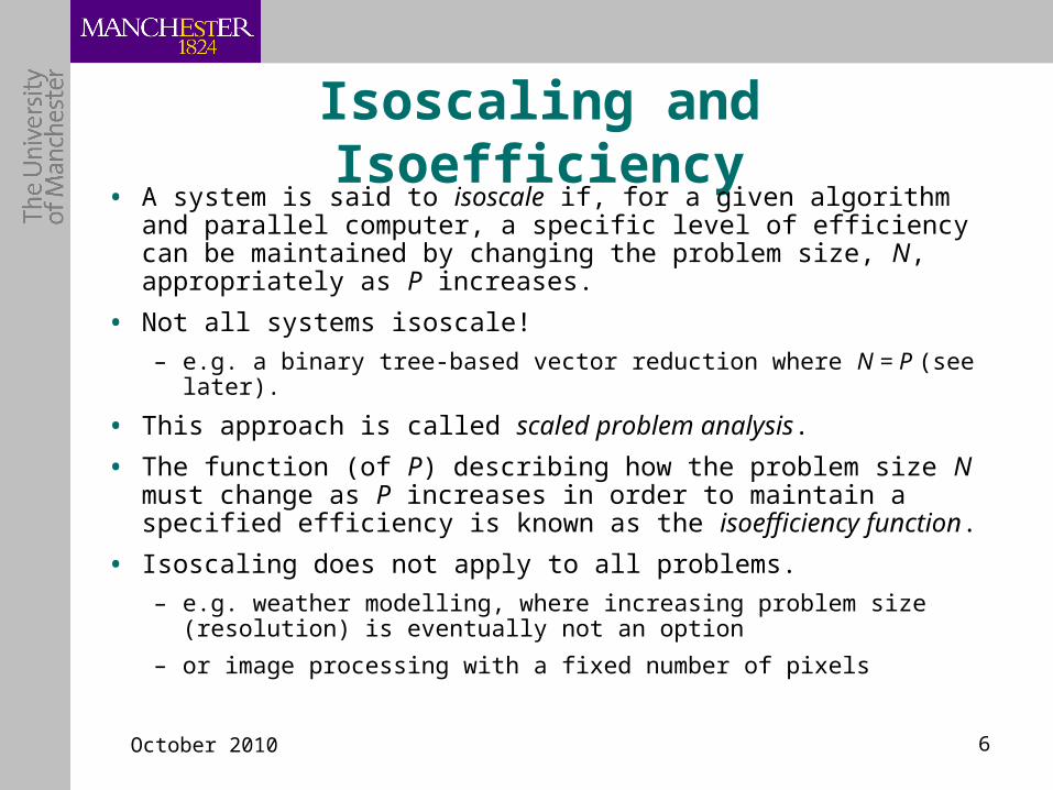
Isoscaling and Isoefficiency• A system is said to isoscale if, for a given algorithm and parallel

computer, a specific level of efficiency can be maintained by changing the problem size, N, appropriately as P increases.

• Not all systems isoscale!

– e.g. a binary tree-based vector reduction where N = P (see later).

• This approach is called scaled problem analysis.

• The function (of P) describing how the problem size N must change as P increases in order to maintain a specified efficiency is known as the isoefficiency function.

• Isoscaling does not apply to all problems.

– e.g. weather modelling, where increasing problem size (resolution) is eventually not an option

– or image processing with a fixed number of pixels

October 2010 7

Weak Scaling• An alternative approach is to keep the problem size per

processor fixed as P increases (total problem size N thus increases linearly with P) and see how the efficiency is affected

– This is known as weak scaling.

• Summary: strong scaling, weak scaling and isoscaling are three different approaches to understanding the scalability of parallel systems (algorithm + machine).

• We will look at an example shortly, but first we need a means of comparing the behaviour of functions, e.g. performance functions and efficiency functions, over their entire domains.

• These concepts will be explored further in lab exercise 2.

October 2010 8

Comparison Functions:Asymptotic Analysis

• Performance models are generally functions of problem size (N) and the number of processors (P).

• We need relatively easy ways to compare models (functions) as N and P vary:

– Model A is ‘at most’ as fast or as big as model B;

– Model A is ‘at least’ as fast or as big as model B;

– Model A is ‘equal’ in performance/size to model B.

• We will see a similar need when comparing efficiencies and in considering scalability.

• These are all examples of comparison functions.

• We are often interested in asymptotic behaviour, i.e. the behaviour as some key parameter (e.g. N or P) increases towards infinity.

October 2010 9

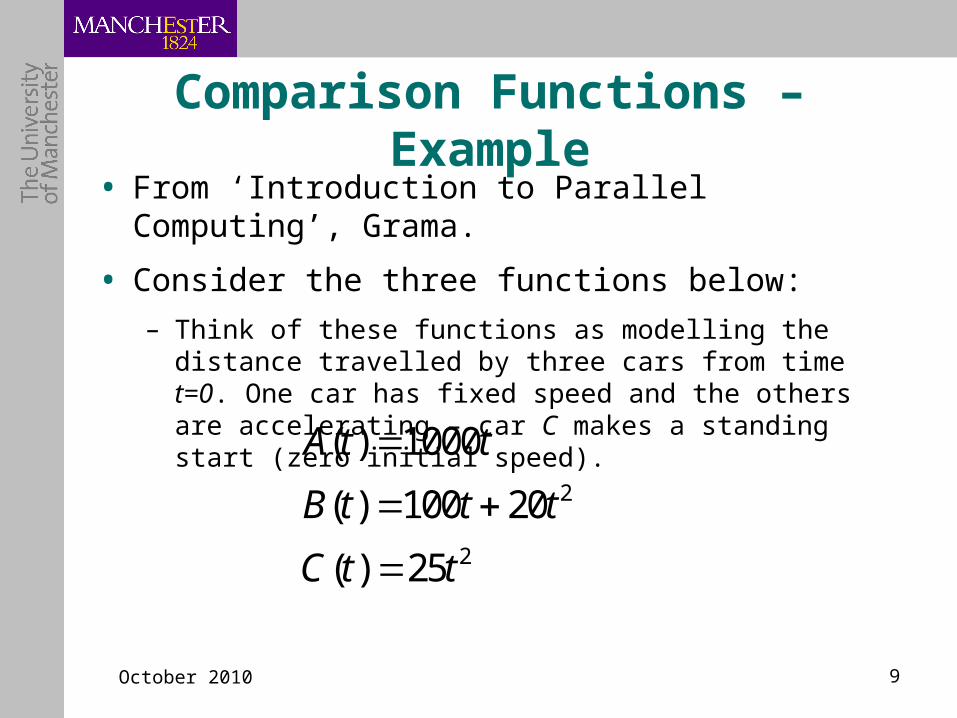
Comparison Functions – Example• From ‘Introduction to Parallel Computing’, Grama.

• Consider the three functions below:

– Think of these functions as modelling the distance travelled by three cars from time t=0. One car has fixed speed and the others are accelerating – car C makes a standing start (zero initial speed).

2

2

( ) 1000

( ) 100 20

( ) 25

A t t

B t t t

C t t

October 2010 10

Graphically

October 2010 11

• We can see that:

– For t > 45, B(t) is always greater than A(t).

– For t > 20, C(t) is always greater than B(t).

– For t > 0, C(t) is always less than 1.25*B(t).

October 2010 12

Introducing ‘big-Oh’ Notation• It is often useful to express a bound on the growth of a particular

function in terms of a simpler function.

• For example, for t > 45, B(t) is always greater than A(t), we can express the relation between A(t) and B(t) using the Ο (Omicron or ‘big-Oh’) notation:

• This means that A(t) is “at most” B(t) beyond some value of t.

• Formally, given functions f(x), g(x),

f(x) = O(g(x))

if there exist positive constants c and x0 such that f(x) ≤ cg(x) for all x ≥ x0 [Definition from JaJa not Grama! – more transparent].

( ) ( ( ))A t B t

October 2010 13

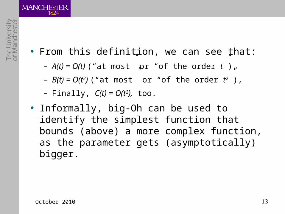
• From this definition, we can see that:

– A(t) = O(t) (“at most” or “of the order t”),

– B(t) = O(t2) (“at most” or “of the order t2”),

– Finally, C(t) = O(t2), too.

• Informally, big-Oh can be used to identify the simplest function that bounds (above) a more complex function, as the parameter gets (asymptotically) bigger.

October 2010 14

Theta and Omega• There are two other useful symbols:

– Omega (Ω) meaning “at least”:

– Theta (Θ) “equals” or “goes as”:

• For formal definitions, see, for example, ‘An Introduction to Parallel Algorithms’ by JaJa or ‘Highly Parallel Computing’ by Almasi and Gottlieb.

• Note that the definitions in Grama et al. are a little misleading!

( ) ( ( ))f x g x

( ) ( ( ))f x g x

October 2010 15

Performance Modelling – Example• The following slides develop performance models for

the example of a vector sum reduction.

• The models are then used to support basic scalability analysis of the resulting parallel systems.

• Consider two parallel systems:– First, a binary tree-based vector sum when the number of

elements (N) is equal to the number of processors (P), N=P.

– Second, a version for which N >> P.

• Develop performance models.– Compare the models.

– Consider the resulting system scalability.

October 2010 16

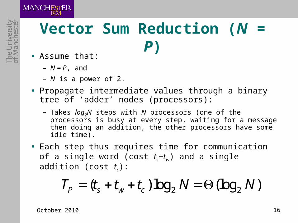
Vector Sum Reduction (N = P)• Assume that:

– N = P, and

– N is a power of 2.

• Propagate intermediate values through a binary tree of ‘adder’ nodes (processors):

– Takes log2N steps with N processors (one of the processors is busy at every step, waiting for a message then doing an addition, the other processors have some idle time).

• Each step thus requires time for communication of a single word (cost ts+tw) and a single addition (cost tc):

2 2( ) log (log )P s w cT t t t N N

October 2010 17

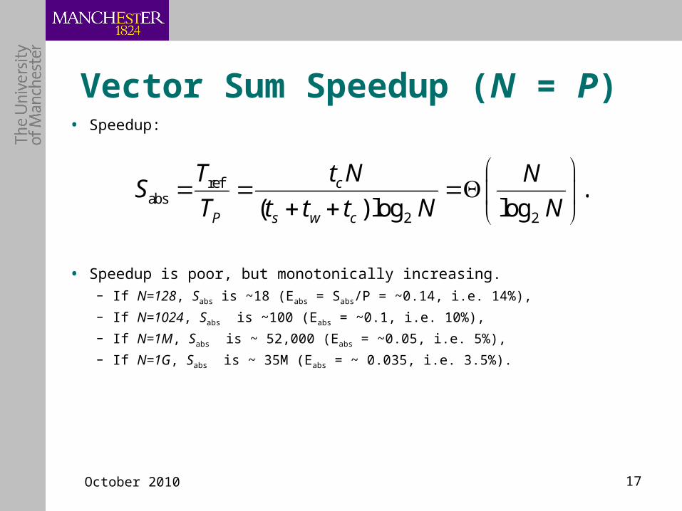
Vector Sum Speedup (N = P)• Speedup:

• Speedup is poor, but monotonically increasing.– If N=128, Sabs is ~18 (Eabs = Sabs/P = ~0.14, i.e. 14%),

– If N=1024, Sabs is ~100 (Eabs = ~0.1, i.e. 10%),

– If N=1M, Sabs is ~ 52,000 (Eabs = ~0.05, i.e. 5%),

– If N=1G, Sabs is ~ 35M (Eabs = ~ 0.035, i.e. 3.5%).

refabs

2 2

.( ) log log

c

P s w c

T t N NS

T t t t N N

October 2010 18

Vector Sum Scalability (N = P)• Efficiency:

• But, N = P in this case, so:

• Strong scaling not ‘good’, as we have seen (Eabs << 0.5).

• Efficiency is monotonically decreasing

– Reaches 50% point, Eabs = 0.5, when log2 P = 2, i.e. when P = 4.

• This does not isoscale, either!

– Eabs gets smaller as P (hence N) increases and P and N must change together.

absabs

2

.log

S NE

P P N

abs2

1.

logE

P

October 2010 19

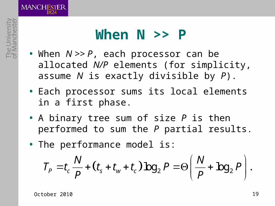
When N >> P• When N >> P, each processor can be allocated N/P

elements (for simplicity, assume N is exactly divisible by P).

• Each processor sums its local elements in a first phase.

• A binary tree sum of size P is then performed to sum the P partial results.

• The performance model is:

2 2log log .P c s w c

N NT t t t t P P

P P

October 2010 20

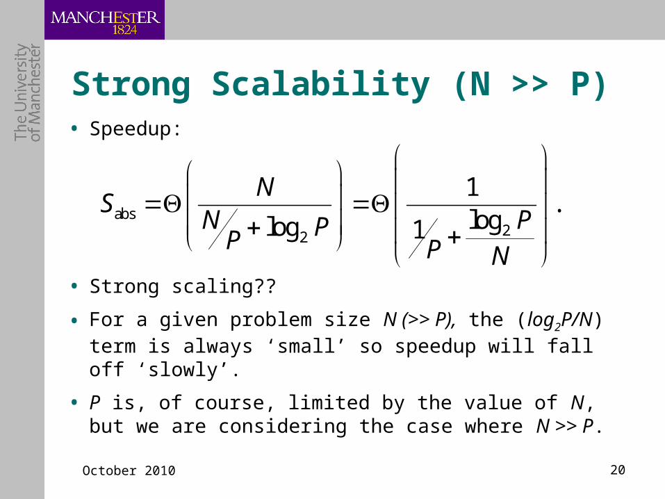
Strong Scalability (N >> P)• Speedup:

• Strong scaling??

• For a given problem size N (>> P), the (log2P/N) term is always ‘small’ so speedup will fall off ‘slowly’.

• P is, of course, limited by the value of N, but we are considering the case where N >> P.

abs22

1.

loglog 1

NS

N PPP P N

October 2010 21

Isoscalability (N >> P)• Efficiency:

• Now, we can always achieve a required efficiency on P processors by a suitable choice of N.

abs2

1.

log1

EP P

N

October 2010 22

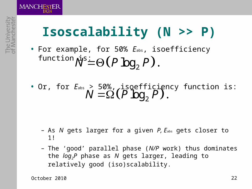
Isoscalability (N >> P)• For example, for 50% Eabs, isoefficiency function is:

• Or, for Eabs > 50%, isoefficiency function is:

– As N gets larger for a given P, Eabs gets closer to 1!

– The ‘good’ parallel phase (N/P work) thus dominates the log2P phase as N gets larger, leading to relatively good (iso)scalability.

2log .N P P

2log .N P P

October 2010 23

Summary of Performance Modelling• Performance modelling provides insight into the behaviour of parallel

systems (parallel algorithms on parallel machines).

• Performance modelling allows the comparison of algorithms and gives insight into their potential scalability.

• Two main forms of scalability:

– Strong scaling (fixed problem size N as P varies)

There is always a limit to strong scaling for real parallel systems (i.e. a value of P at which efficiency falls below an acceptable limit).

– Isoscaling (the ability to maintain a specified level of efficiency by changing N as P varies).

Not all parallel systems isoscale.

• Asymptotic (‘big-Oh’) analysis makes comparison easier, but BEWARE the constants!

• Weak scaling is related to isoscaling – aim to maintain a fixed problem size per processor as P changes and look at the effect on efficiency.