COMP1 5.4. Representing Sound in a ComputerSound Course book - pages 124 - 131.

COMP1 5.4. Representing Sound in a

Computer

Course book - pages 124 - 131

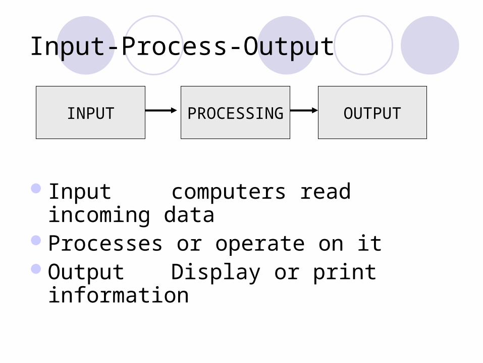
Input-Process-Output

Input computers read incoming data

Processes or operate on itOutput Display or print information

INPUT PROCESSING OUTPUT

Data versus Information

Datathe raw material which a computer

accepts as input and then processes into useful information

Informationprocessed data that provides

understandable and useful information

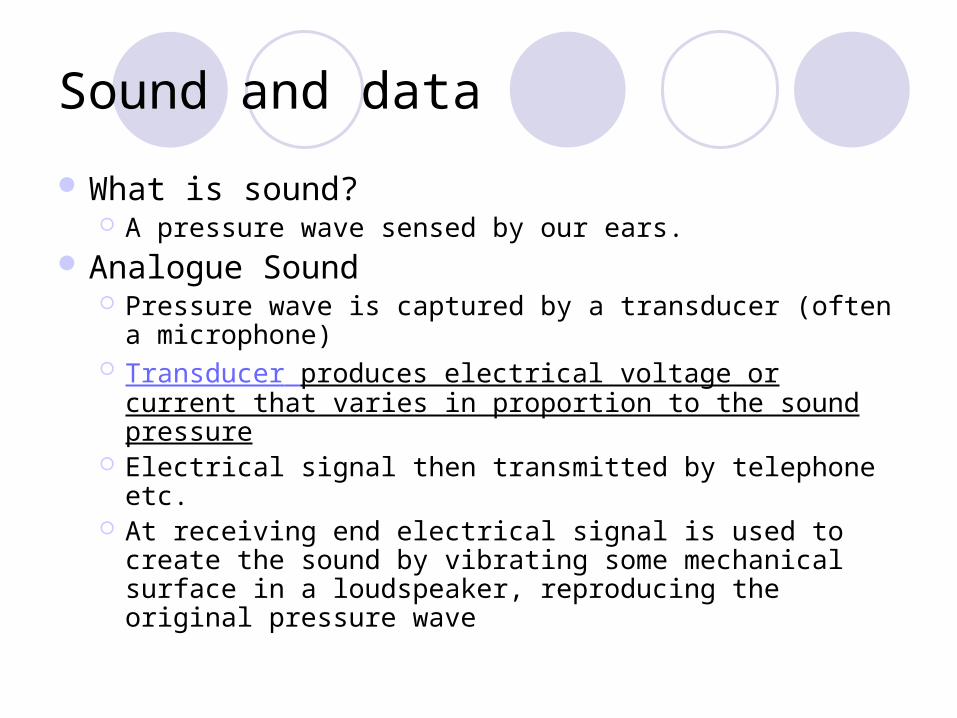
Sound and data

What is sound? A pressure wave sensed by our ears.

Analogue Sound Pressure wave is captured by a transducer (often a

microphone) Transducer produces electrical voltage or current that

varies in proportion to the sound pressure Electrical signal then transmitted by telephone etc. At receiving end electrical signal is used to create the

sound by vibrating some mechanical surface in a loudspeaker, reproducing the original pressure wave

Coding Schemes

Data is represented using various coding schemes. Different forms of information:

ASCII Unicode Binary Numbers Gray Code Boolean Values Digitised Sound Bit-mapped graphics / pixel

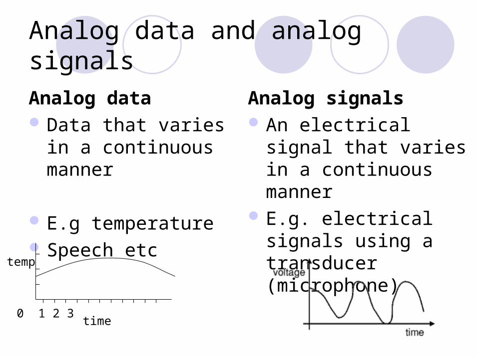
Analog data and analog signals

Analog data Data that varies in a

continuous manner

E.g temperature Speech etc

Analog signals An electrical signal that

varies in a continuous manner

E.g. electrical signals using a transducer (microphone)

temp

time0 1 2 3

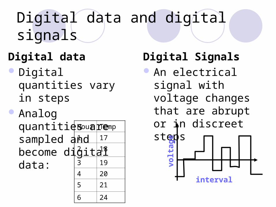
Digital data and digital signals

Digital data Digital quantities vary

in steps Analog quantities are

sampled and become digital data:

Digital Signals An electrical signal

with voltage changes that are abrupt or in discreet steps

Hour Temp

1 17

2 18

3 19

4 20

5 21

6 24

voltage

interval

Sound- key terms

WavelengthSampling rateFrequencyIntervalBit rate

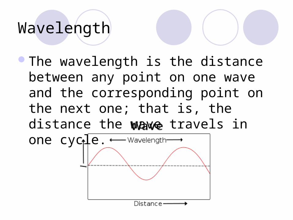
Wavelength

The wavelength is the distance between any point on one wave and the corresponding point on the next one; that is, the distance the wave travels in one cycle.

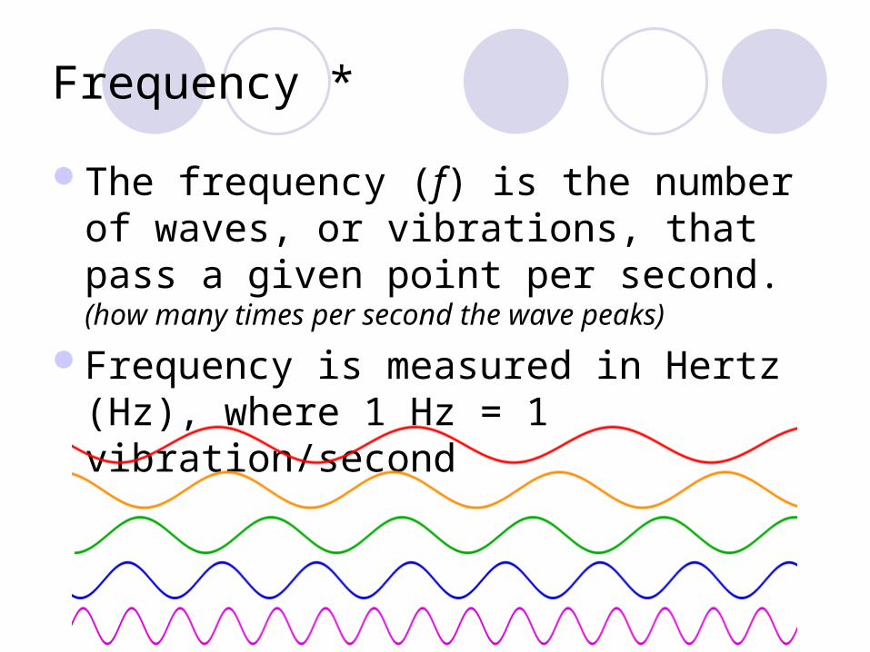
Frequency *

The frequency (f) is the number of waves, or vibrations, that pass a given point per second. (how many times per second the wave peaks)

Frequency is measured in Hertz (Hz), where 1 Hz = 1 vibration/second

Amplitude

The larger the amplitude, the louder the tone; the smaller the amplitude, the softer the tone. Loudness is measure in decibels.

Smaller amplitude (A1) = softer sound Larger amplitude (A2) = louder sound

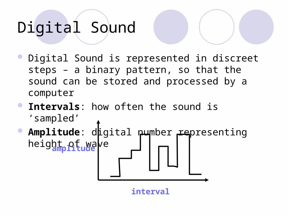
Digital Sound

Digital Sound is represented in discreet steps – a binary pattern, so that the sound can be stored and processed by a computer

Intervals: how often the sound is ‘sampled’ Amplitude: digital number representing height of wave

amplitude

interval

Converting Analogue to Digital Sound *

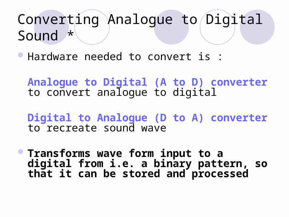
Hardware needed to convert is :

Analogue to Digital (A to D) converter to convert analogue to digital

Digital to Analogue (D to A) converter to recreate sound wave

Transforms wave form input to a digital from i.e. a binary pattern, so that it can be stored and processed

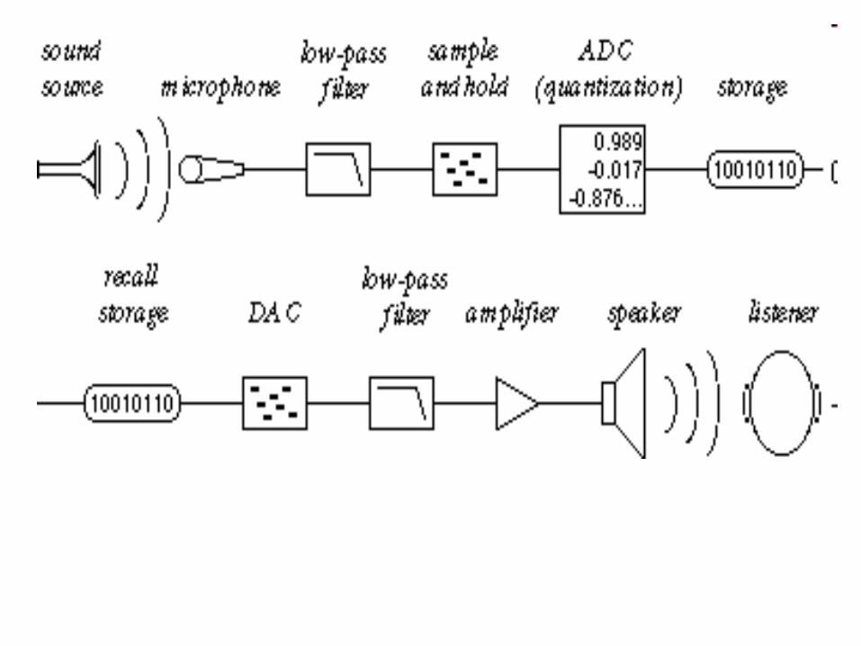
A-to-D Converter

Analogue signals can be converted into digital form by using the variations in frequency (pitch) and the variation in amplitude (loudness) of the sound

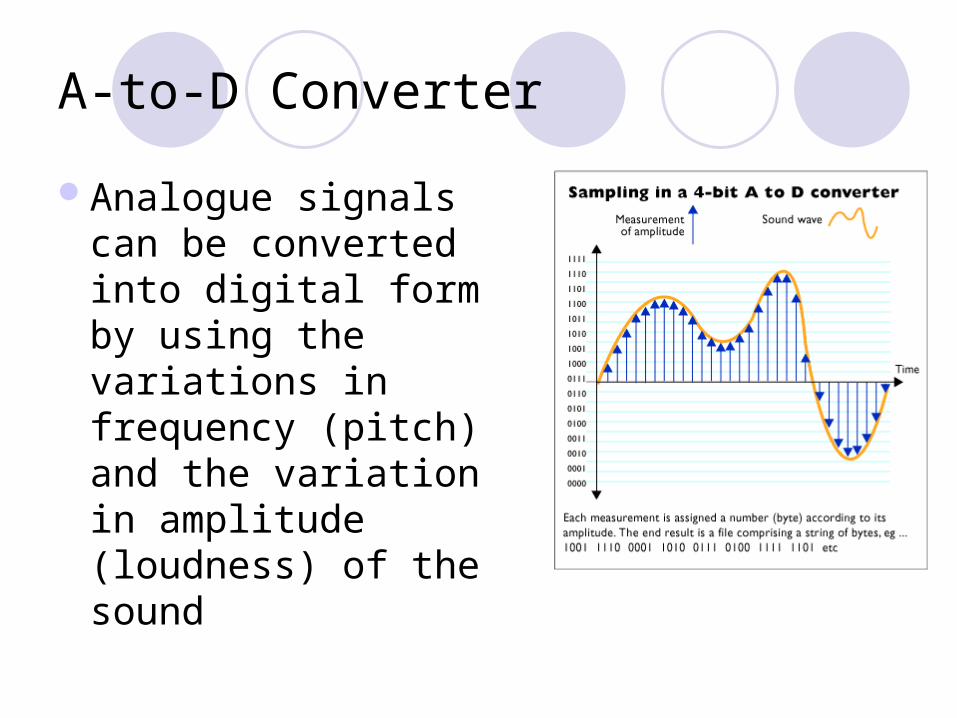
A-to-D Converter and quantisation noise

Height of analogue wave form can be sampled at regular spaced intervals, with the height being represented by say a 16 bit codeSampling resolution: The number of bits used to store one sound sampleSampling rate: * the frequency at which samples are taken, the higher the sampling rate the more faithful the sound is represented

The conversion has three stages:

Sampling of amplitude signals (PAM pulses) – sampling rate at least twice the highest frequency in the analog signal (Nyquist Theorem)

Digitizing of the amplitude signals (PCM pulses) - PAM samples are quantised- the height of each PAM pulse is assigned a digital value.

Encoding of the stream of bits . Each value is translated into e.g. a 7-bit number (8th bit is sign)

Quantisation noise/error

The difference between the original amplitude and its sampled value is known as quantisation noise.

Quantisation error is due either to rounding or truncation

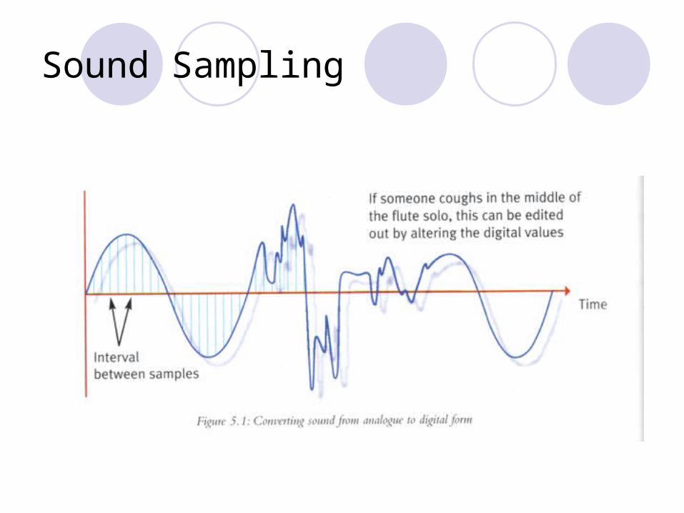
Sound Sampling

Sampled Sound and Nyquist’s Theorem

Sampling at 1 time per cycle

Sampling at 1.5 times per cycle

Sampling at 2 times per cycle

Digital Audio

Is typically created by taking 16-bit samples over a spectrum of 44.1 KHz.

Stereo sound doubles the number of samples taken, with 44,100 samples per second taking 32 bits each.

CD quality sound requires 1,4 million bits of data per second.

Sound Synthesis (sound generation)

Sound can be generated using analogue or digital techniques

Digital sound generation Numbers representing sound waves are

manipulated Sampled sounds as well as pure tones and

arithmetic operations are carried out on the bit patterns representing the sound

MIDI

Musical Instrument Digital InterfaceIs a particular form of serial interface

built into or added to the parts of an electronic music system E.g. Microphone, electronic keyboard with

MIDI

It does not store sound waves but a digital representation of the notes to be played.

Streaming audio

E.g. RealPlayer Streaming client receives the audio data – put

into a buffer until it’s used. The client player reads the data from the buffer

and plays it. As long as player is not trying to access data

that hasn’t been received, the streaming is successful.

Streaming avoids the need to download and store large files. It also prevents copying.

Factors that affect the quality of recorded sound

1) frequency range of the sound which is sampled/played back, The Loudness war*

2) the sample rate at which the sound is initially sampled in the recording process

3) the conversions that occur after sampling to reproduce the final digital sound (characterised by its bitrate) which gets played back.

File formats

WAV format – supported by Windows. 1 minute requires 2.5Mb of disk space

MPEG (Mp2, mpa, mp3, mp4) – is a compression algorithm. It removes frequencies that the brain and ear will not miss (psychoacoustic). 1 minute MP3 requires .25Mb

Example

Analog signal of frequency 1,000 Hz is converted to PCM digital signal by sampling at a frequency of 2,000Hz (2000 samples per second). Each sample uses 8 bits.

How many Bytes are required for the PCM-coded result if recording 10 seconds of analog signal?

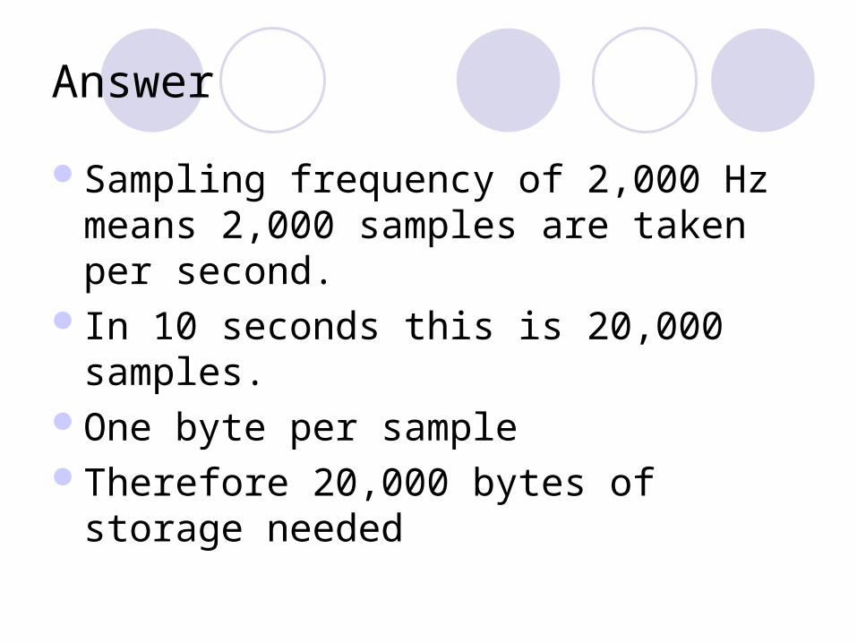
Answer

Sampling frequency of 2,000 Hz means 2,000 samples are taken per second.

In 10 seconds this is 20,000 samples.One byte per sampleTherefore 20,000 bytes of storage needed

Activity -

In pairsEach group creates 2 questions on topic

with a marking schemeQuestion to the rest of the class