COMP 551 – Applied Machine Learning Lecture 6: Performance evaluation. Model assessment and selection. Unless otherwise noted, all material posted for this course are copyright of the instructors, and cannot be reused or reposted without the instructors’ written permission. Instructor: Herke van Hoof ([email protected]) Slides mostly by: Joelle Pineau Class web page: www.cs.mcgill.ca/~hvanho2/comp551

Welcome message from author
This document is posted to help you gain knowledge. Please leave a comment to let me know what you think about it! Share it to your friends and learn new things together.
Transcript
COMP 551 – Applied Machine LearningLecture 6: Performance evaluation. Model
assessment and selection.
Unless otherwise noted, all material posted for this course are copyright of the instructors, and cannot be reused or reposted without the instructors’ written permission.
Instructor: Herke van Hoof ([email protected])
Slides mostly by: Joelle Pineau
Class web page: www.cs.mcgill.ca/~hvanho2/comp551
Joelle Pineau2
Today’s quiz (on myCourses)
• Quiz on classification on myCourses
COMP-551: Applied Machine Learning
Joelle Pineau3
Project questions
• Best place to ask questions: MyCourses forum
• Others can browse questions/answers so everyone can learn
from them
• If you have a specific problem, try to visit the office hour of the
responsible TA (mentioned on exercise) – they are best placed
to help you!
COMP-551: Applied Machine Learning
Joelle Pineau4
Project 1 hand in
• Original data: Jan 26
• We’ll accept submissions until Jan 29, noon (strict deadline)
– Hardcopy (in box) & code/data (on mycourses)
• Late policy: within 1 week late will be accepted with 30% penalty
• Caution: project 2 will still be available from Jan 26!
• Hand-in box:
– Opposite 317 in McConnell building
COMP-551: Applied Machine Learning
Joelle Pineau5
Evaluating performance
• Different objectives:
– Selecting the right model for a problem.
– Testing performance of a new algorithm.
– Evaluating impact on a new application.
COMP-551: Applied Machine Learning
Joelle Pineau6
Performance metrics for classification
• Not all errors have equal impact!
• There are different types of mistakes, particularly in the classification setting.
COMP-551: Applied Machine Learning
Joelle Pineau7
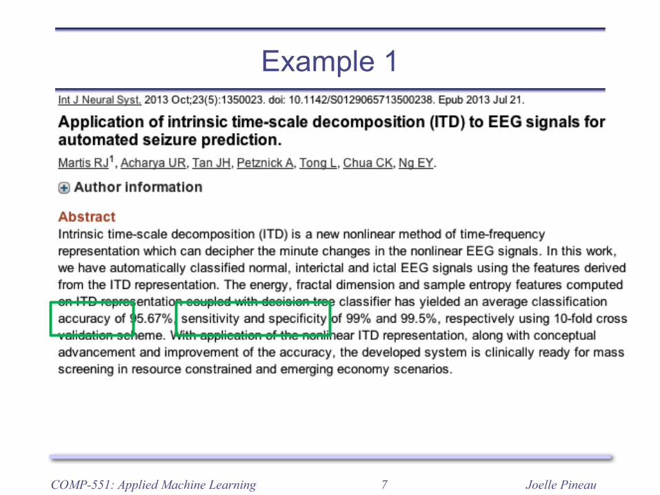
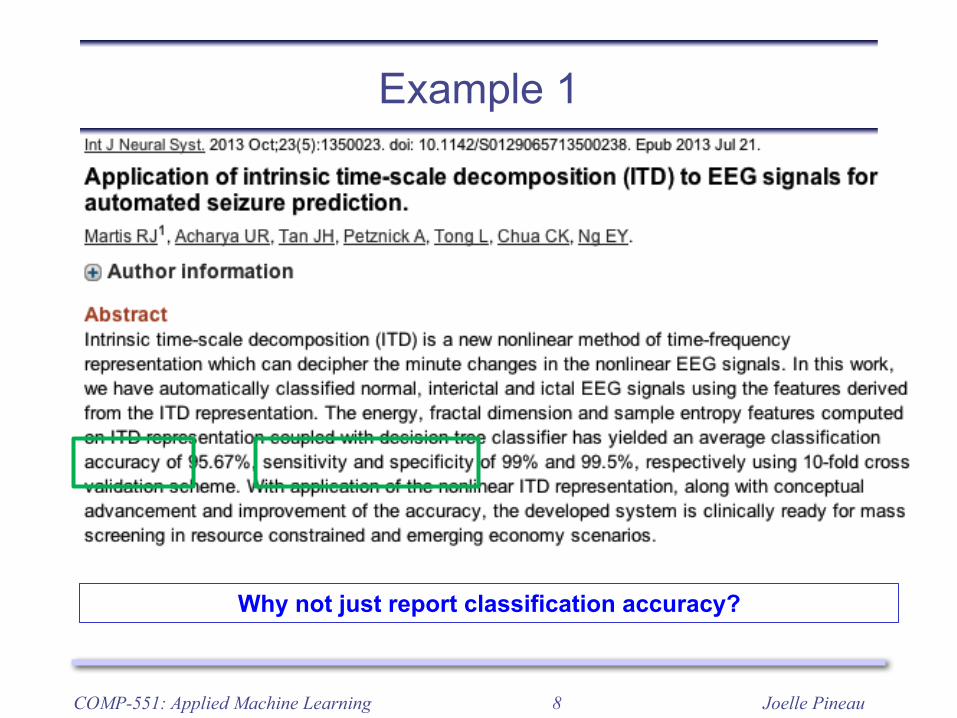
Example 1
COMP-551: Applied Machine Learning
Joelle Pineau8
Example 1
COMP-551: Applied Machine Learning
Why not just report classification accuracy?
Joelle Pineau9
Performance metrics for classification
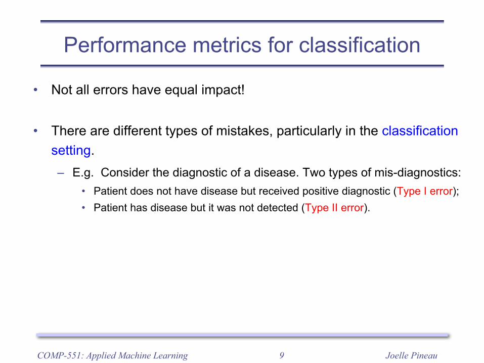
• Not all errors have equal impact!
• There are different types of mistakes, particularly in the classification setting.– E.g. Consider the diagnostic of a disease. Two types of mis-diagnostics:
• Patient does not have disease but received positive diagnostic (Type I error);• Patient has disease but it was not detected (Type II error).
COMP-551: Applied Machine Learning
Joelle Pineau10
Performance metrics for classification
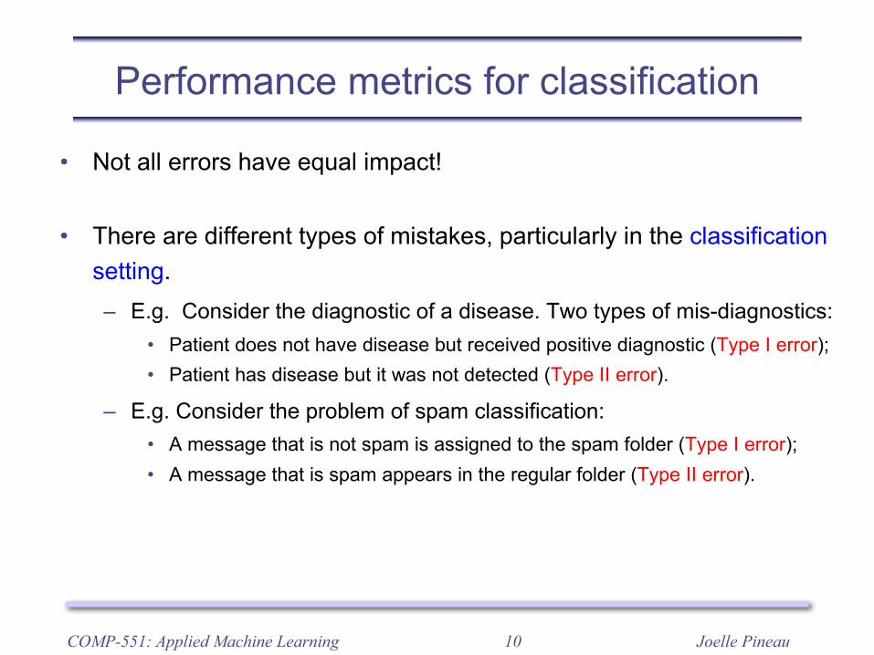
• Not all errors have equal impact!
• There are different types of mistakes, particularly in the classification setting.– E.g. Consider the diagnostic of a disease. Two types of mis-diagnostics:
• Patient does not have disease but received positive diagnostic (Type I error);• Patient has disease but it was not detected (Type II error).
– E.g. Consider the problem of spam classification:• A message that is not spam is assigned to the spam folder (Type I error);• A message that is spam appears in the regular folder (Type II error).
COMP-551: Applied Machine Learning
Joelle Pineau11
Performance metrics for classification
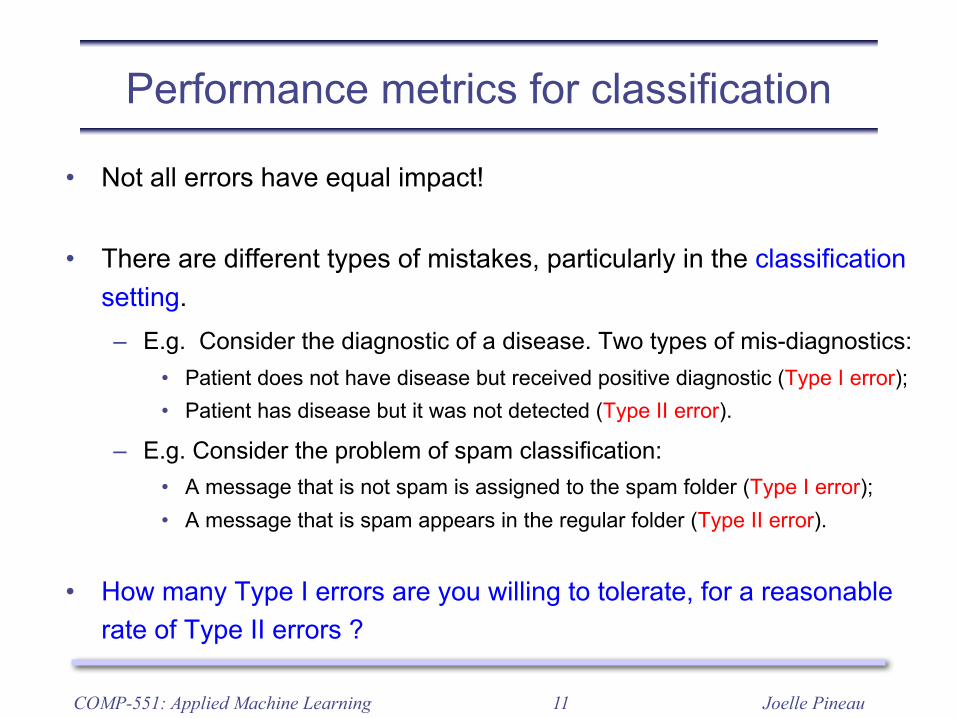
• Not all errors have equal impact!
• There are different types of mistakes, particularly in the classification setting.– E.g. Consider the diagnostic of a disease. Two types of mis-diagnostics:
• Patient does not have disease but received positive diagnostic (Type I error);• Patient has disease but it was not detected (Type II error).
– E.g. Consider the problem of spam classification:• A message that is not spam is assigned to the spam folder (Type I error);• A message that is spam appears in the regular folder (Type II error).
• How many Type I errors are you willing to tolerate, for a reasonable rate of Type II errors ?
COMP-551: Applied Machine Learning
Joelle Pineau12
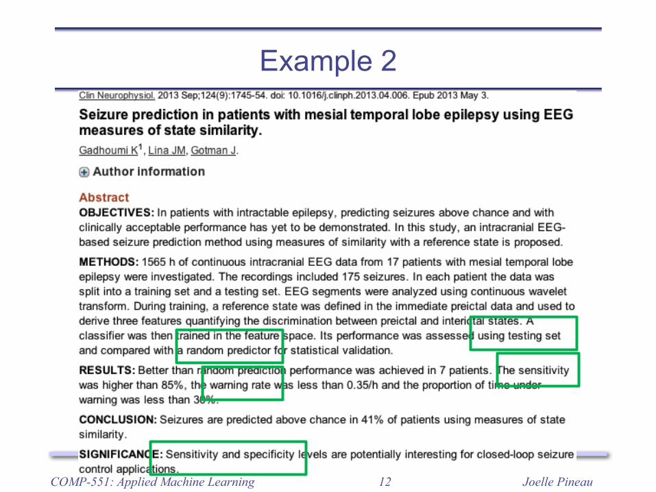
Example 2
COMP-551: Applied Machine Learning
Joelle Pineau13
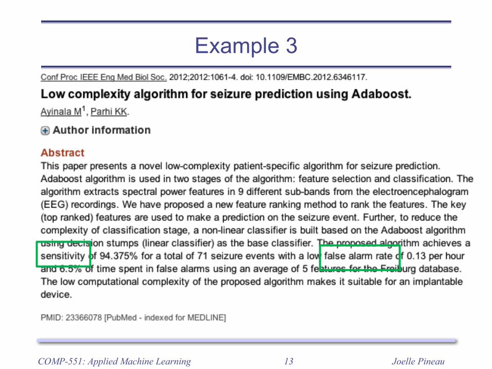
Example 3
COMP-551: Applied Machine Learning
Joelle Pineau14
Terminology
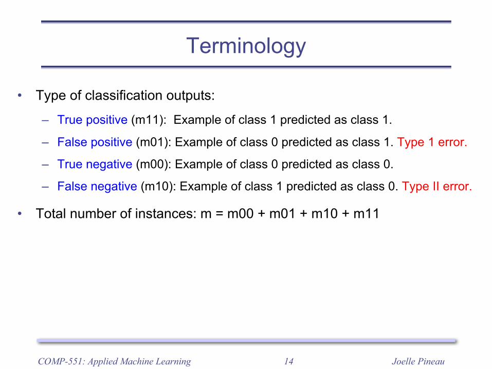
• Type of classification outputs:
– True positive (m11): Example of class 1 predicted as class 1.
– False positive (m01): Example of class 0 predicted as class 1. Type 1 error.
– True negative (m00): Example of class 0 predicted as class 0.
– False negative (m10): Example of class 1 predicted as class 0. Type II error.
• Total number of instances: m = m00 + m01 + m10 + m11
COMP-551: Applied Machine Learning
Joelle Pineau15
Terminology
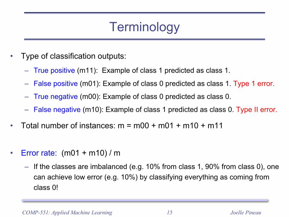
• Type of classification outputs:
– True positive (m11): Example of class 1 predicted as class 1.
– False positive (m01): Example of class 0 predicted as class 1. Type 1 error.
– True negative (m00): Example of class 0 predicted as class 0.
– False negative (m10): Example of class 1 predicted as class 0. Type II error.
• Total number of instances: m = m00 + m01 + m10 + m11
• Error rate: (m01 + m10) / m– If the classes are imbalanced (e.g. 10% from class 1, 90% from class 0), one
can achieve low error (e.g. 10%) by classifying everything as coming from class 0!
COMP-551: Applied Machine Learning
Joelle Pineau16
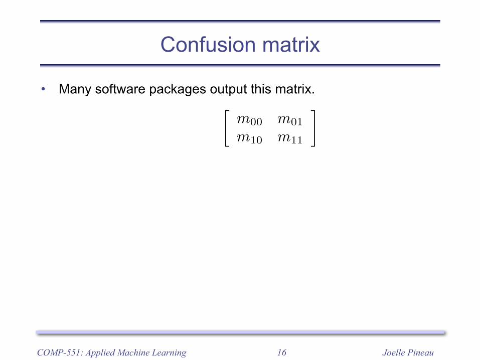
Confusion matrix
• Many software packages output this matrix.
COMP-551: Applied Machine Learning
Confusion matrix
• Confusion matrix gives more information than error rate:
m00 m01
m10 m11
�
• Many software packages (eg. Weka) output this matrix
• Varying the parameter of the algorithm produces a curve
COMP-652, Lecture 12 - October 18, 2012 11

Joelle Pineau17
Confusion matrix
• Many software packages output this matrix.
• Be careful! Sometimes the format is slightly different(E.g. http://en.wikipedia.org/wiki/Precision_and_recall#Definition_.28classification_context.29)
COMP-551: Applied Machine Learning
Confusion matrix
• Confusion matrix gives more information than error rate:
m00 m01
m10 m11
�
• Many software packages (eg. Weka) output this matrix
• Varying the parameter of the algorithm produces a curve
COMP-652, Lecture 12 - October 18, 2012 11
Joelle Pineau18
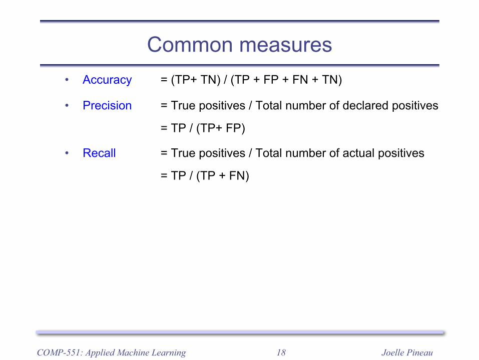
Common measures• Accuracy = (TP+ TN) / (TP + FP + FN + TN)
• Precision = True positives / Total number of declared positives
= TP / (TP+ FP)
• Recall = True positives / Total number of actual positives
= TP / (TP + FN)
COMP-551: Applied Machine Learning
Joelle Pineau19
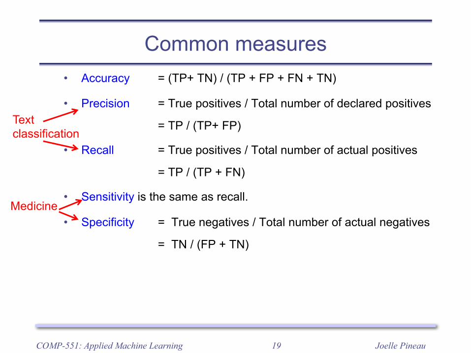
Common measures• Accuracy = (TP+ TN) / (TP + FP + FN + TN)
• Precision = True positives / Total number of declared positives
= TP / (TP+ FP)
• Recall = True positives / Total number of actual positives
= TP / (TP + FN)
• Sensitivity is the same as recall.
• Specificity = True negatives / Total number of actual negatives
= TN / (FP + TN)
COMP-551: Applied Machine Learning
Textclassification
Medicine
Joelle Pineau20
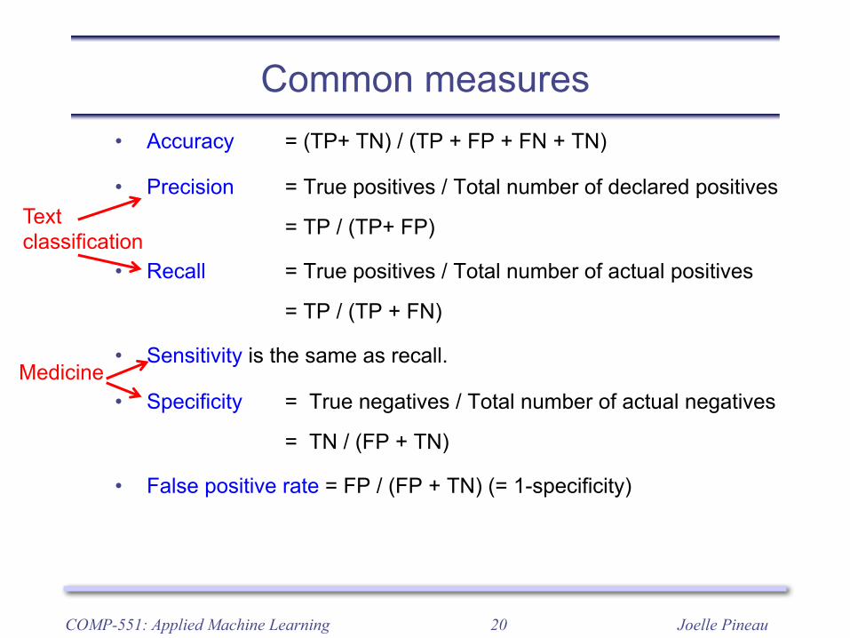
Common measures• Accuracy = (TP+ TN) / (TP + FP + FN + TN)
• Precision = True positives / Total number of declared positives
= TP / (TP+ FP)
• Recall = True positives / Total number of actual positives
= TP / (TP + FN)
• Sensitivity is the same as recall.
• Specificity = True negatives / Total number of actual negatives
= TN / (FP + TN)
• False positive rate = FP / (FP + TN) (= 1-specificity)
COMP-551: Applied Machine Learning
Textclassification
Medicine
Joelle Pineau21
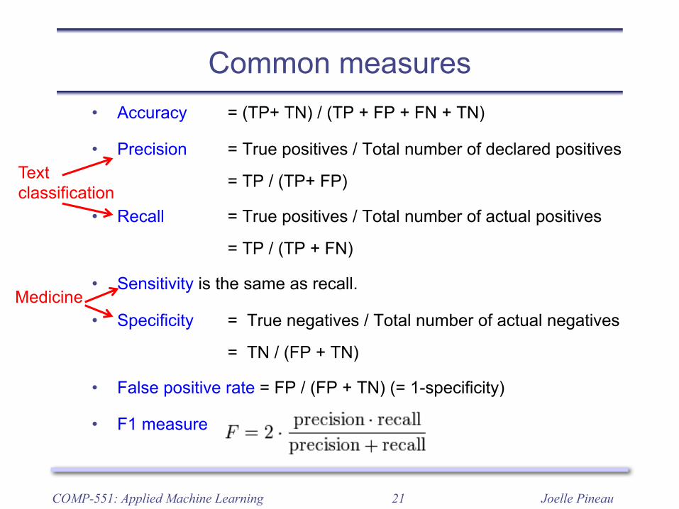
Common measures• Accuracy = (TP+ TN) / (TP + FP + FN + TN)
• Precision = True positives / Total number of declared positives
= TP / (TP+ FP)
• Recall = True positives / Total number of actual positives
= TP / (TP + FN)
• Sensitivity is the same as recall.
• Specificity = True negatives / Total number of actual negatives
= TN / (FP + TN)
• False positive rate = FP / (FP + TN) (= 1-specificity)
• F1 measure
COMP-551: Applied Machine Learning
Textclassification
Medicine
Joelle Pineau22
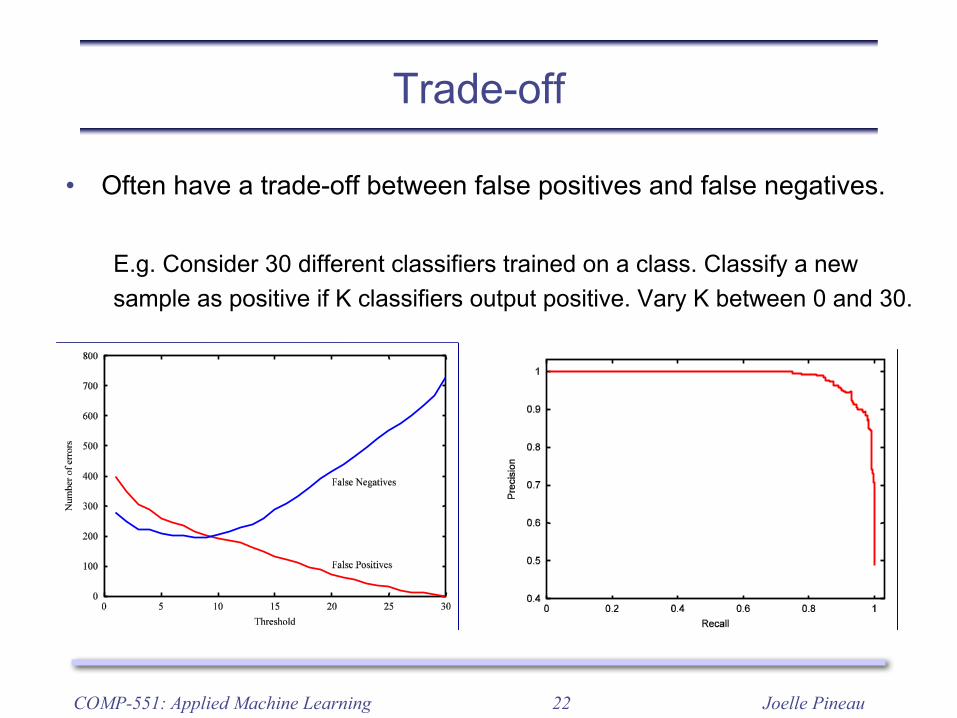
Trade-off
• Often have a trade-off between false positives and false negatives.
E.g. Consider 30 different classifiers trained on a class. Classify a new sample as positive if K classifiers output positive. Vary K between 0 and 30.
COMP-551: Applied Machine Learning
Example: Tree bagging
• 30 decision trees, classify an example as positive if K trees classify it aspositive
• Vary K between 0 and 30
!"#$%&'()*+),'-./.01)23''/)!"#$%&'()*+),'-./.01)23''/)-01/234-2',)56)5#77.17-01/234-2',)56)5#77.17
8&#//.96)#/)%0/.2.:').9);)042)09)*+)23''/)8&#//.96)#/)%0/.2.:').9);)042)09)*+)23''/)%3',.-2)%0/.2.:'<))=#36);<%3',.-2)%0/.2.:'<))=#36);<
COMP-652, Lecture 12 - October 18, 2012 12
Precision-recall
• Similar concept to AUC curves, but used in retrieval tasks
• Precision is true positive / total number of documents retrieved
• Recall is true positives / all positives
• In medical applications we use instead sensitivity and selectivity, whichare the recall for the two classes
!"#$%&%'()*#$+,,)-"+./!"#$%&%'()*#$+,,)-"+./!,'0)"#$+,,)'()/'"%1'(0+,)+2%&3)."#$%&%'()'()!,'0)"#$+,,)'()/'"%1'(0+,)+2%&3)."#$%&%'()'()4#"0%$+,)+2%&3)+(5)4+"6)0/#)0/"#&/',5)7'")8+9%(:)4#"0%$+,)+2%&3)+(5)4+"6)0/#)0/"#&/',5)7'")8+9%(:).'&%0%4#)."#5%$0%'(&);'")4+"6)<=.'&%0%4#)."#5%$0%'(&);'")4+"6)<=
COMP-652, Lecture 12 - October 18, 2012 17
Joelle Pineau23
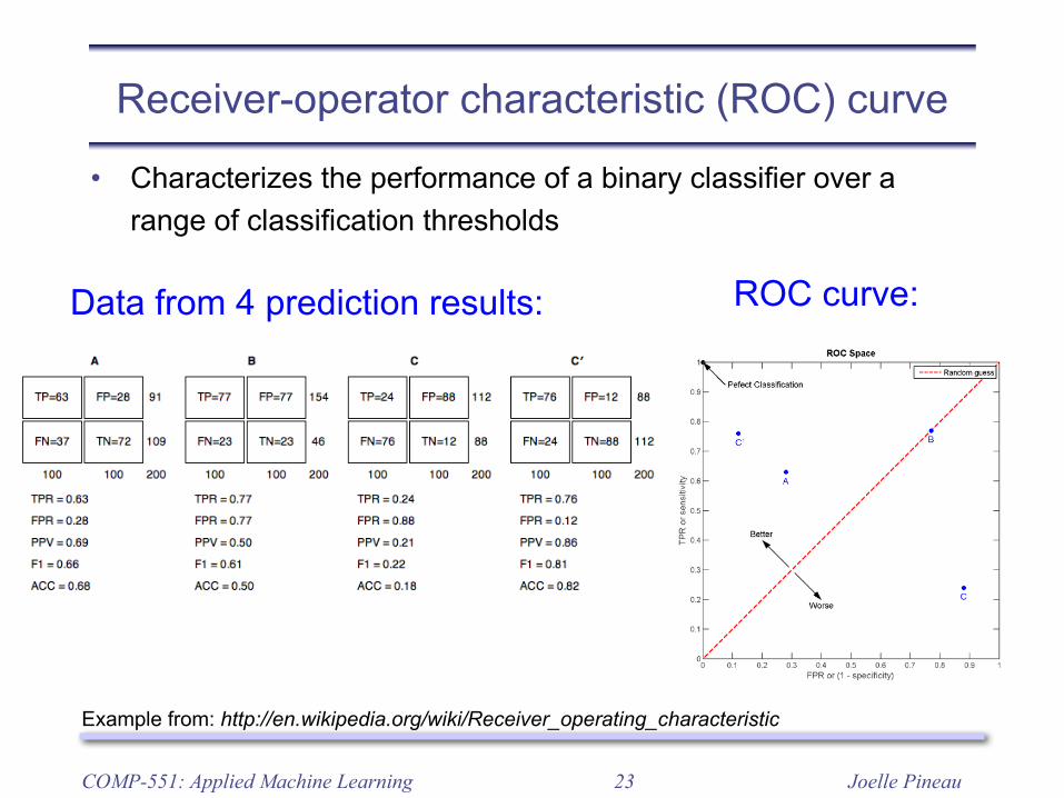
Receiver-operator characteristic (ROC) curve
• Characterizes the performance of a binary classifier over a range of classification thresholds
COMP-551: Applied Machine Learning
Data from 4 prediction results: ROC curve:
Example from: http://en.wikipedia.org/wiki/Receiver_operating_characteristic
Joelle Pineau24
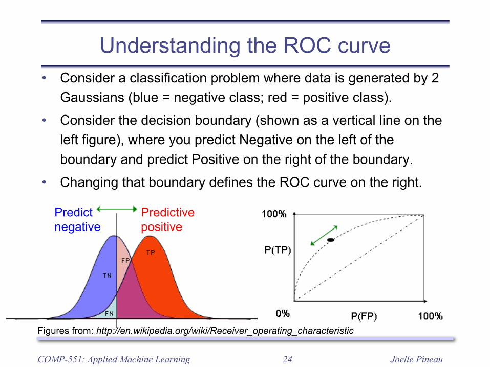
Understanding the ROC curve• Consider a classification problem where data is generated by 2
Gaussians (blue = negative class; red = positive class).• Consider the decision boundary (shown as a vertical line on the
left figure), where you predict Negative on the left of the boundary and predict Positive on the right of the boundary.
• Changing that boundary defines the ROC curve on the right.
COMP-551: Applied Machine Learning
Predictivepositive
Predictnegative
Figures from: http://en.wikipedia.org/wiki/Receiver_operating_characteristic
Joelle Pineau25
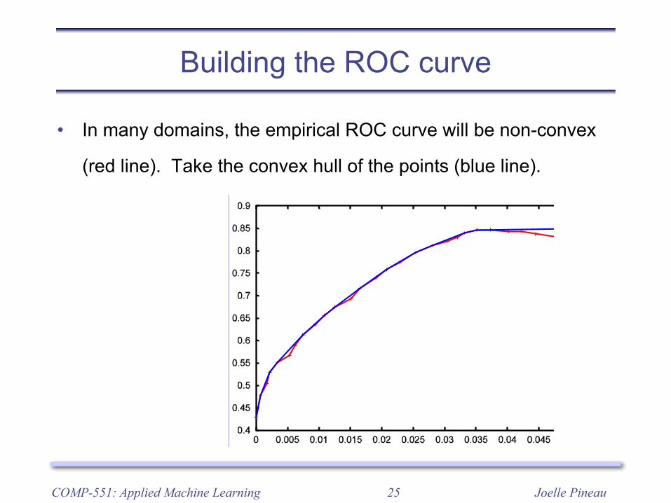
Building the ROC curve
• In many domains, the empirical ROC curve will be non-convex
(red line). Take the convex hull of the points (blue line).
COMP-551: Applied Machine Learning
ROC convex hull
• Suppose we have two hypotheses h1 and h2 along the ROC curve.
• We can always use h1 with probability p and h2 with probability (1 � p)and the performance will interpolate between the two
• So we can always match any point on the convex hull of an empiricalROC curve !"#$#%&'()$*+,,!"#$#%&'()$*+,,
!"#$#%&'()$*+,,
"-./.&0,$!"#$#+-'(
COMP-652, Lecture 12 - October 18, 2012 15
Joelle Pineau26
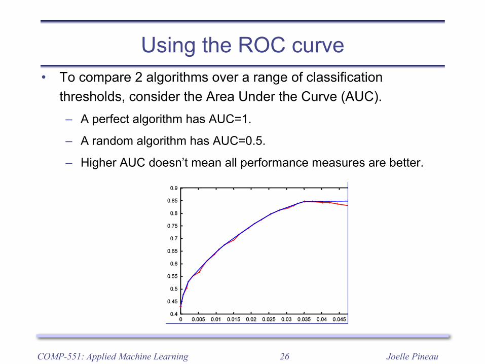
Using the ROC curve• To compare 2 algorithms over a range of classification
thresholds, consider the Area Under the Curve (AUC).– A perfect algorithm has AUC=1.
– A random algorithm has AUC=0.5.
– Higher AUC doesn’t mean all performance measures are better.
COMP-551: Applied Machine Learning
ROC convex hull
• Suppose we have two hypotheses h1 and h2 along the ROC curve.
• We can always use h1 with probability p and h2 with probability (1 � p)and the performance will interpolate between the two
• So we can always match any point on the convex hull of an empiricalROC curve !"#$#%&'()$*+,,!"#$#%&'()$*+,,
!"#$#%&'()$*+,,
"-./.&0,$!"#$#+-'(
COMP-652, Lecture 12 - October 18, 2012 15
Joelle Pineau27
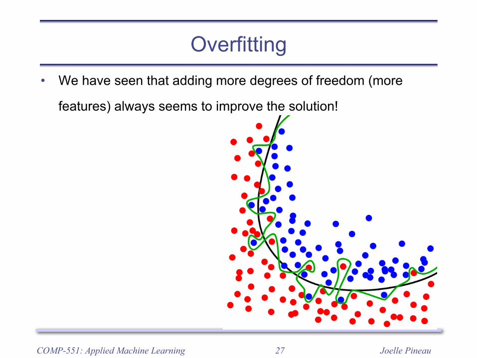
Overfitting• We have seen that adding more degrees of freedom (more
features) always seems to improve the solution!
COMP-551: Applied Machine Learning
Joelle Pineau28
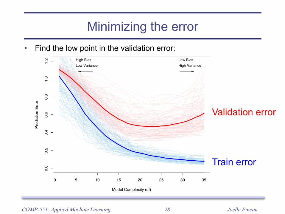
Minimizing the error• Find the low point in the validation error:
COMP-551: Applied Machine Learning
220 7. Model Assessment and Selection
0 5 10 15 20 25 30 35
0.0
0.2
0.4
0.6
0.8
1.0
1.2
Model Complexity (df)
Pred
ictio
n Er
ror
High Bias Low BiasHigh VarianceLow Variance
FIGURE 7.1. Behavior of test sample and training sample error as the modelcomplexity is varied. The light blue curves show the training error err, while thelight red curves show the conditional test error ErrT for 100 training sets of size50 each, as the model complexity is increased. The solid curves show the expectedtest error Err and the expected training error E[err].
Test error, also referred to as generalization error, is the prediction errorover an independent test sample
ErrT = E[L(Y, f̂(X))|T ] (7.2)
where both X and Y are drawn randomly from their joint distribution(population). Here the training set T is fixed, and test error refers to theerror for this specific training set. A related quantity is the expected pre-diction error (or expected test error)
Err = E[L(Y, f̂(X))] = E[ErrT ]. (7.3)
Note that this expectation averages over everything that is random, includ-ing the randomness in the training set that produced f̂ .
Figure 7.1 shows the prediction error (light red curves) ErrT for 100simulated training sets each of size 50. The lasso (Section 3.4.2) was usedto produce the sequence of fits. The solid red curve is the average, andhence an estimate of Err.
Estimation of ErrT will be our goal, although we will see that Err ismore amenable to statistical analysis, and most methods effectively esti-mate the expected error. It does not seem possible to estimate conditional
Train error
Validation error
Joelle Pineau29
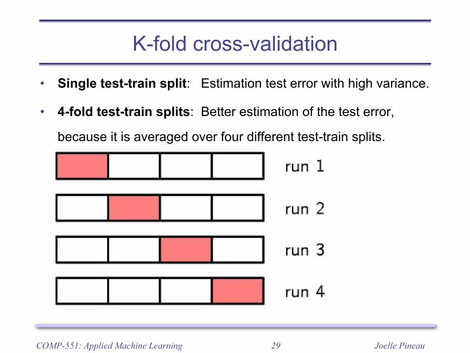
K-fold cross-validation
• Single test-train split: Estimation test error with high variance.
• 4-fold test-train splits: Better estimation of the test error,
because it is averaged over four different test-train splits.
COMP-551: Applied Machine Learning
Joelle Pineau30
K-fold cross-validation
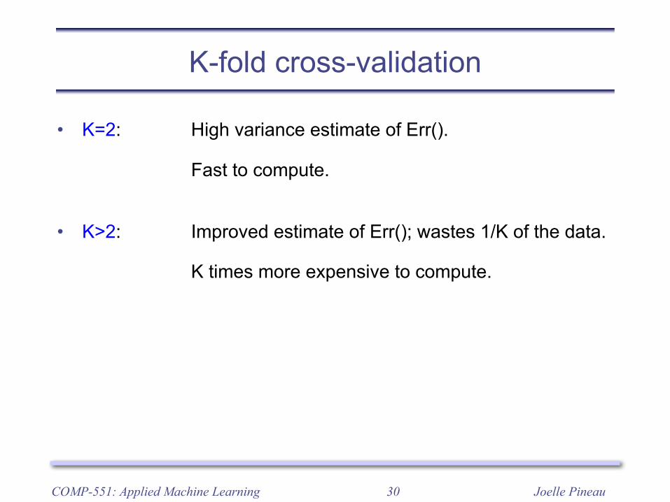
• K=2: High variance estimate of Err().
Fast to compute.
• K>2: Improved estimate of Err(); wastes 1/K of the data.
K times more expensive to compute.
COMP-551: Applied Machine Learning
Joelle Pineau31
K-fold cross-validation
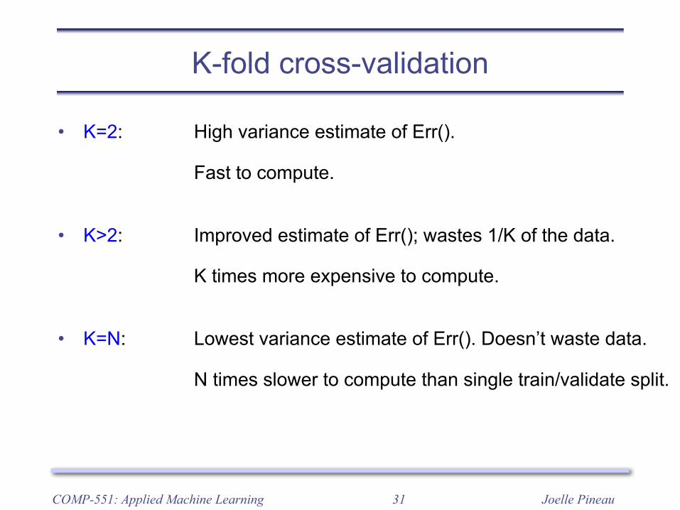
• K=2: High variance estimate of Err().
Fast to compute.
• K>2: Improved estimate of Err(); wastes 1/K of the data.
K times more expensive to compute.
• K=N: Lowest variance estimate of Err(). Doesn’t waste data.
N times slower to compute than single train/validate split.
COMP-551: Applied Machine Learning
Joelle Pineau32
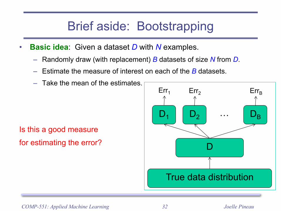
Brief aside: Bootstrapping• Basic idea: Given a dataset D with N examples.
– Randomly draw (with replacement) B datasets of size N from D.– Estimate the measure of interest on each of the B datasets.– Take the mean of the estimates.
Is this a good measurefor estimating the error?
COMP-551: Applied Machine Learning
True data distribution
D
D1 D2 DB…
Err1 Err2 ErrB
Joelle Pineau33
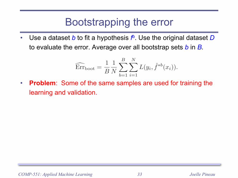
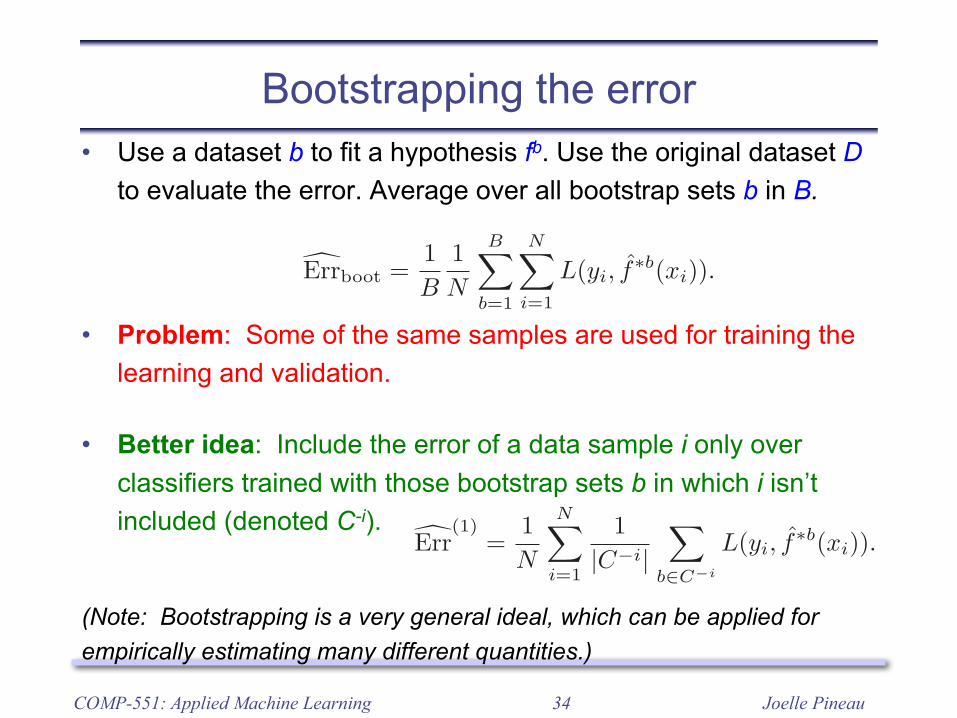
Bootstrapping the error• Use a dataset b to fit a hypothesis fb. Use the original dataset D
to evaluate the error. Average over all bootstrap sets b in B.
• Problem: Some of the same samples are used for training the learning and validation.
COMP-551: Applied Machine Learning
250 7. Model Assessment and Selection
Bootstrap
Bootstrap
replications
samples
sampleTrainingZ = (z1, z2, . . . , zN )
Z∗1 Z∗2 Z∗B
S(Z∗1) S(Z∗2) S(Z∗B)
FIGURE 7.12. Schematic of the bootstrap process. We wish to assess the sta-tistical accuracy of a quantity S(Z) computed from our dataset. B training setsZ∗b, b = 1, . . . , B each of size N are drawn with replacement from the originaldataset. The quantity of interest S(Z) is computed from each bootstrap trainingset, and the values S(Z∗1), . . . , S(Z∗B) are used to assess the statistical accuracyof S(Z).
where S̄∗ =!
b S(Z∗b)/B. Note that "Var[S(Z)] can be thought of as a
Monte-Carlo estimate of the variance of S(Z) under sampling from theempirical distribution function F̂ for the data (z1, z2, . . . , zN ).
How can we apply the bootstrap to estimate prediction error? One ap-proach would be to fit the model in question on a set of bootstrap samples,and then keep track of how well it predicts the original training set. Iff̂∗b(xi) is the predicted value at xi, from the model fitted to the bth boot-strap dataset, our estimate is
"Errboot =1
B
1
N
B#
b=1
N#
i=1
L(yi, f̂∗b(xi)). (7.54)
However, it is easy to see that"Errboot does not provide a good estimate ingeneral. The reason is that the bootstrap datasets are acting as the trainingsamples, while the original training set is acting as the test sample, andthese two samples have observations in common. This overlap can makeoverfit predictions look unrealistically good, and is the reason that cross-validation explicitly uses non-overlapping data for the training and testsamples. Consider for example a 1-nearest neighbor classifier applied to atwo-class classification problem with the same number of observations in
Joelle Pineau34
Bootstrapping the error• Use a dataset b to fit a hypothesis fb. Use the original dataset D
to evaluate the error. Average over all bootstrap sets b in B.
• Problem: Some of the same samples are used for training the learning and validation.
• Better idea: Include the error of a data sample i only over classifiers trained with those bootstrap sets b in which i isn’t included (denoted C-i).
(Note: Bootstrapping is a very general ideal, which can be applied for empirically estimating many different quantities.)
COMP-551: Applied Machine Learning
250 7. Model Assessment and Selection
Bootstrap
Bootstrap
replications
samples
sampleTrainingZ = (z1, z2, . . . , zN )
Z∗1 Z∗2 Z∗B
S(Z∗1) S(Z∗2) S(Z∗B)
FIGURE 7.12. Schematic of the bootstrap process. We wish to assess the sta-tistical accuracy of a quantity S(Z) computed from our dataset. B training setsZ∗b, b = 1, . . . , B each of size N are drawn with replacement from the originaldataset. The quantity of interest S(Z) is computed from each bootstrap trainingset, and the values S(Z∗1), . . . , S(Z∗B) are used to assess the statistical accuracyof S(Z).
where S̄∗ =!
b S(Z∗b)/B. Note that "Var[S(Z)] can be thought of as a
Monte-Carlo estimate of the variance of S(Z) under sampling from theempirical distribution function F̂ for the data (z1, z2, . . . , zN ).
How can we apply the bootstrap to estimate prediction error? One ap-proach would be to fit the model in question on a set of bootstrap samples,and then keep track of how well it predicts the original training set. Iff̂∗b(xi) is the predicted value at xi, from the model fitted to the bth boot-strap dataset, our estimate is
"Errboot =1
B
1
N
B#
b=1
N#
i=1
L(yi, f̂∗b(xi)). (7.54)
However, it is easy to see that"Errboot does not provide a good estimate ingeneral. The reason is that the bootstrap datasets are acting as the trainingsamples, while the original training set is acting as the test sample, andthese two samples have observations in common. This overlap can makeoverfit predictions look unrealistically good, and is the reason that cross-validation explicitly uses non-overlapping data for the training and testsamples. Consider for example a 1-nearest neighbor classifier applied to atwo-class classification problem with the same number of observations in
7.11 Bootstrap Methods 251
each class, in which the predictors and class labels are in fact independent.Then the true error rate is 0.5. But the contributions to the bootstrapestimate!Errboot will be zero unless the observation i does not appear in thebootstrap sample b. In this latter case it will have the correct expectation0.5. Now
Pr{observation i ∈ bootstrap sample b} = 1−"1− 1
N
#N
≈ 1− e−1
= 0.632. (7.55)
Hence the expectation of !Errboot is about 0.5 × 0.368 = 0.184, far belowthe correct error rate 0.5.
By mimicking cross-validation, a better bootstrap estimate can be ob-tained. For each observation, we only keep track of predictions from boot-strap samples not containing that observation. The leave-one-out bootstrapestimate of prediction error is defined by
!Err(1)
=1
N
N$
i=1
1
|C−i|$
b∈C−i
L(yi, f̂∗b(xi)). (7.56)
Here C−i is the set of indices of the bootstrap samples b that do not contain
observation i, and |C−i| is the number of such samples. In computing!Err(1)
,we either have to choose B large enough to ensure that all of the |C−i| aregreater than zero, or we can just leave out the terms in (7.56) correspondingto |C−i|’s that are zero.
The leave-one out bootstrap solves the overfitting problem suffered by!Errboot, but has the training-set-size bias mentioned in the discussion ofcross-validation. The average number of distinct observations in each boot-strap sample is about 0.632 ·N , so its bias will roughly behave like that oftwofold cross-validation. Thus if the learning curve has considerable slopeat sample size N/2, the leave-one out bootstrap will be biased upward asan estimate of the true error.
The “.632 estimator” is designed to alleviate this bias. It is defined by
!Err(.632)
= .368 · err + .632 ·!Err(1)
. (7.57)
The derivation of the .632 estimator is complex; intuitively it pulls theleave-one out bootstrap estimate down toward the training error rate, andhence reduces its upward bias. The use of the constant .632 relates to (7.55).The .632 estimator works well in “light fitting” situations, but can break
down in overfit ones. Here is an example due to Breiman et al. (1984).Suppose we have two equal-size classes, with the targets independent ofthe class labels, and we apply a one-nearest neighbor rule. Then err = 0,
Joelle Pineau35
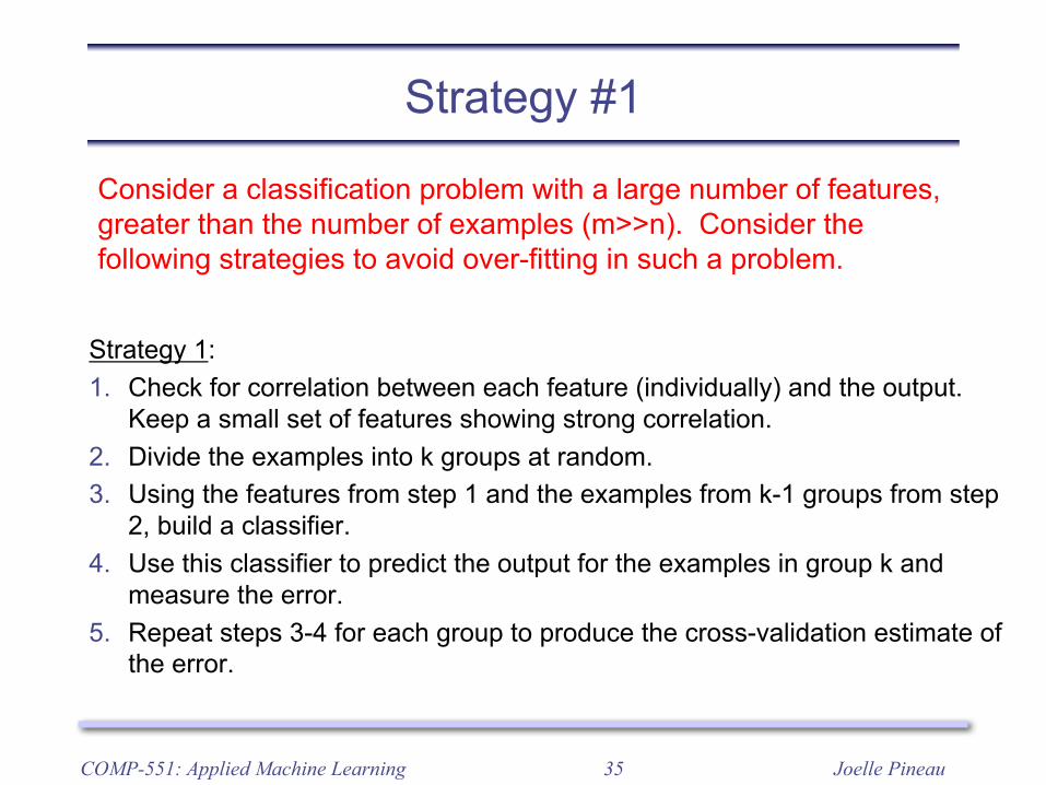
Strategy #1
Strategy 1:1. Check for correlation between each feature (individually) and the output.
Keep a small set of features showing strong correlation.2. Divide the examples into k groups at random.3. Using the features from step 1 and the examples from k-1 groups from step
2, build a classifier.4. Use this classifier to predict the output for the examples in group k and
measure the error.5. Repeat steps 3-4 for each group to produce the cross-validation estimate of
the error.
COMP-551: Applied Machine Learning
Consider a classification problem with a large number of features, greater than the number of examples (m>>n). Consider the following strategies to avoid over-fitting in such a problem.
Joelle Pineau36
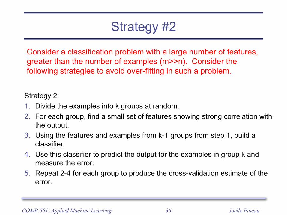
Strategy #2
Strategy 2:1. Divide the examples into k groups at random.2. For each group, find a small set of features showing strong correlation with
the output.3. Using the features and examples from k-1 groups from step 1, build a
classifier.4. Use this classifier to predict the output for the examples in group k and
measure the error.5. Repeat 2-4 for each group to produce the cross-validation estimate of the
error.
COMP-551: Applied Machine Learning
Consider a classification problem with a large number of features, greater than the number of examples (m>>n). Consider the following strategies to avoid over-fitting in such a problem.
Joelle Pineau37
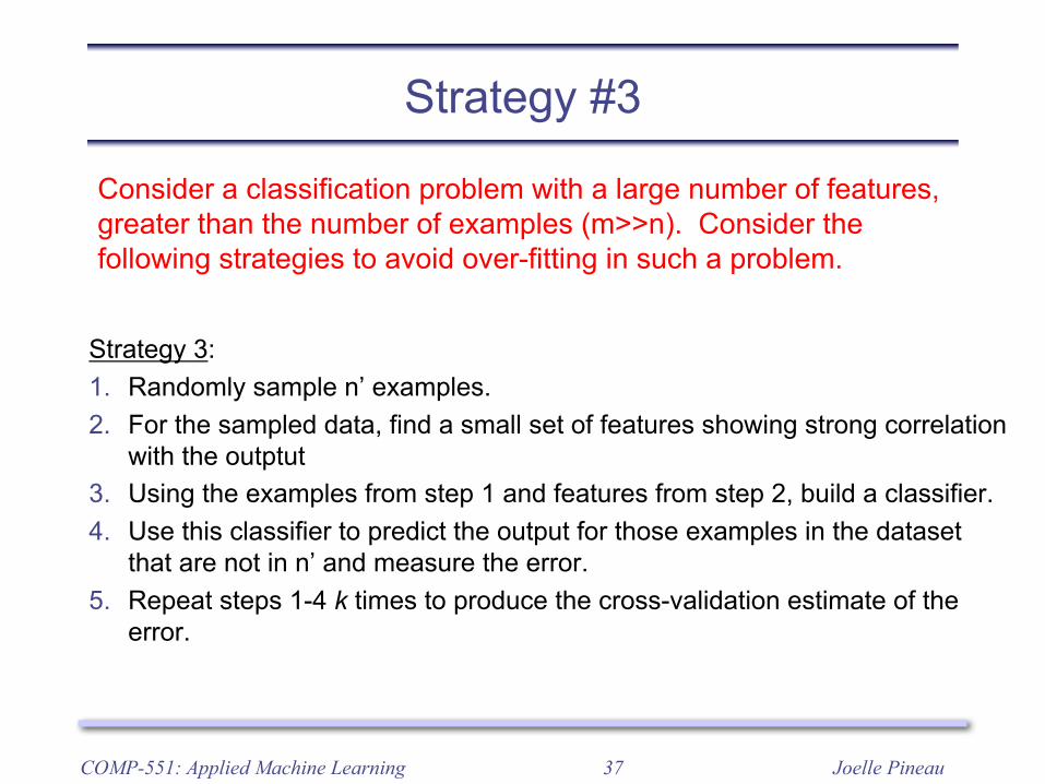
Strategy #3
Strategy 3:1. Randomly sample n’ examples.2. For the sampled data, find a small set of features showing strong correlation
with the outptut3. Using the examples from step 1 and features from step 2, build a classifier.4. Use this classifier to predict the output for those examples in the dataset
that are not in n’ and measure the error.5. Repeat steps 1-4 k times to produce the cross-validation estimate of the
error.
COMP-551: Applied Machine Learning
Consider a classification problem with a large number of features, greater than the number of examples (m>>n). Consider the following strategies to avoid over-fitting in such a problem.
Joelle Pineau38
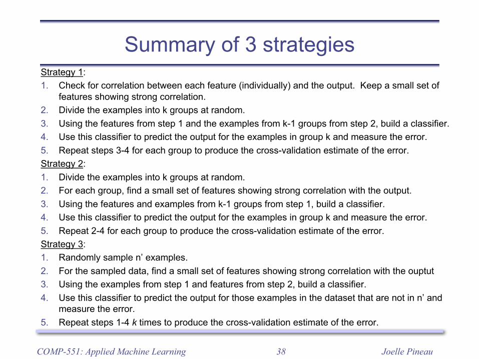
Summary of 3 strategiesStrategy 1:1. Check for correlation between each feature (individually) and the output. Keep a small set of
features showing strong correlation.2. Divide the examples into k groups at random.3. Using the features from step 1 and the examples from k-1 groups from step 2, build a classifier.4. Use this classifier to predict the output for the examples in group k and measure the error.5. Repeat steps 3-4 for each group to produce the cross-validation estimate of the error.Strategy 2:1. Divide the examples into k groups at random.2. For each group, find a small set of features showing strong correlation with the output.3. Using the features and examples from k-1 groups from step 1, build a classifier.4. Use this classifier to predict the output for the examples in group k and measure the error.5. Repeat 2-4 for each group to produce the cross-validation estimate of the error.Strategy 3:1. Randomly sample n’ examples.2. For the sampled data, find a small set of features showing strong correlation with the ouptut3. Using the examples from step 1 and features from step 2, build a classifier.4. Use this classifier to predict the output for those examples in the dataset that are not in n’ and
measure the error.5. Repeat steps 1-4 k times to produce the cross-validation estimate of the error.
COMP-551: Applied Machine Learning
Joelle Pineau39
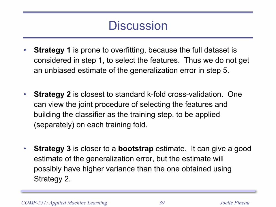
Discussion
• Strategy 1 is prone to overfitting, because the full dataset is considered in step 1, to select the features. Thus we do not get an unbiased estimate of the generalization error in step 5.
• Strategy 2 is closest to standard k-fold cross-validation. One can view the joint procedure of selecting the features and building the classifier as the training step, to be applied (separately) on each training fold.
• Strategy 3 is closer to a bootstrap estimate. It can give a good estimate of the generalization error, but the estimate will possibly have higher variance than the one obtained using Strategy 2.
COMP-551: Applied Machine Learning
Joelle Pineau40
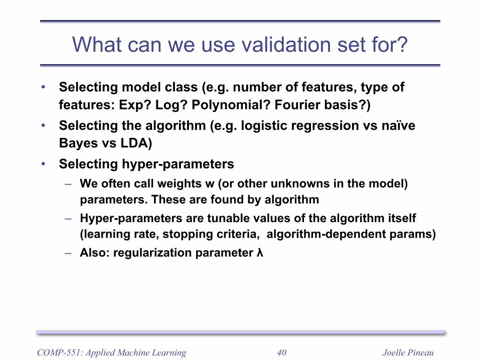
What can we use validation set for?
• Selecting model class (e.g. number of features, type of features: Exp? Log? Polynomial? Fourier basis?)
• Selecting the algorithm (e.g. logistic regression vs naïve Bayes vs LDA)
• Selecting hyper-parameters– We often call weights w (or other unknowns in the model)
parameters. These are found by algorithm– Hyper-parameters are tunable values of the algorithm itself
(learning rate, stopping criteria, algorithm-dependent params)– Also: regularization parameter λ
COMP-551: Applied Machine Learning
Joelle Pineau41
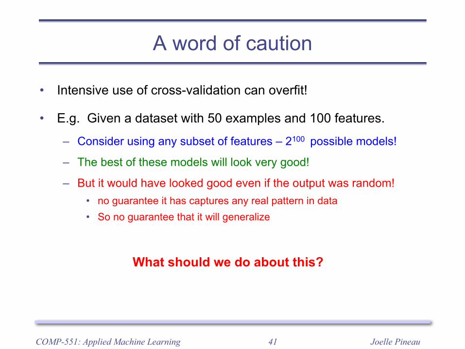
A word of caution
• Intensive use of cross-validation can overfit!
• E.g. Given a dataset with 50 examples and 100 features.
– Consider using any subset of features – 2100 possible models!
– The best of these models will look very good!
– But it would have looked good even if the output was random!• no guarantee it has captures any real pattern in data• So no guarantee that it will generalize
What should we do about this?
COMP-551: Applied Machine Learning
Joelle Pineau42
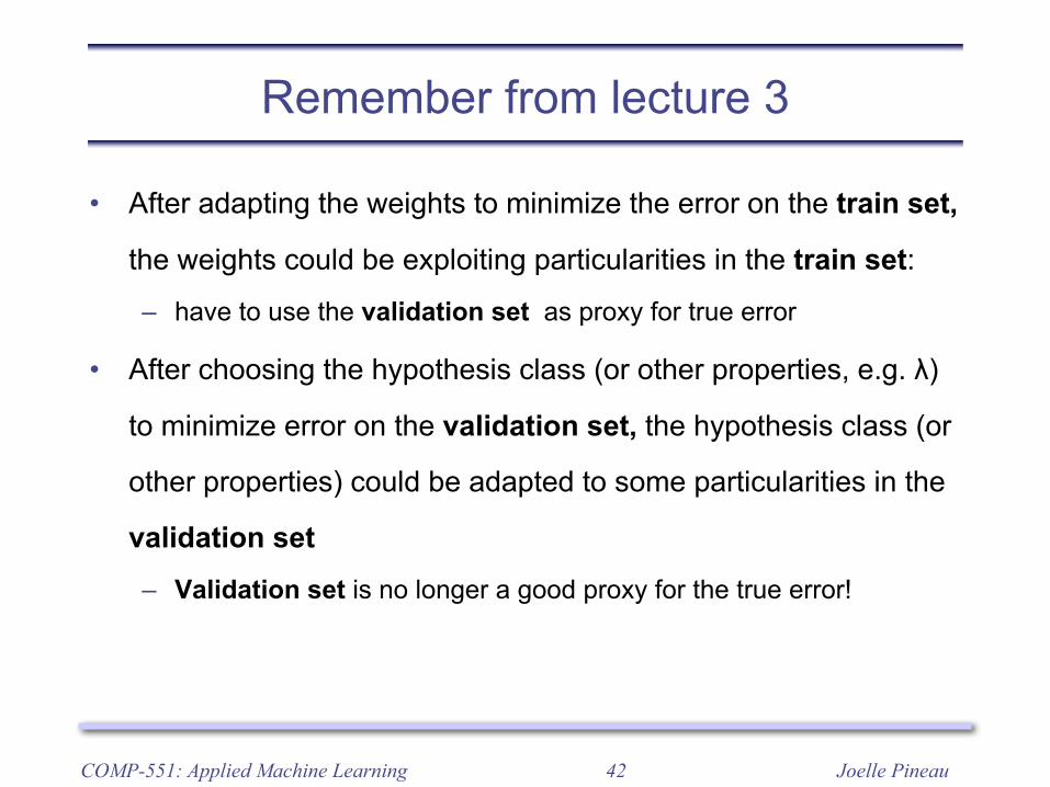
Remember from lecture 3
• After adapting the weights to minimize the error on the train set,
the weights could be exploiting particularities in the train set:– have to use the validation set as proxy for true error
• After choosing the hypothesis class (or other properties, e.g. λ)
to minimize error on the validation set, the hypothesis class (or
other properties) could be adapted to some particularities in the
validation set– Validation set is no longer a good proxy for the true error!
COMP-551: Applied Machine Learning
Joelle Pineau43
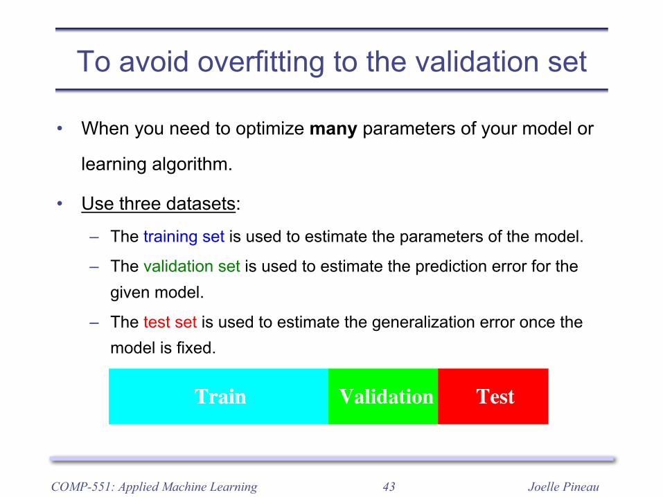
To avoid overfitting to the validation set
• When you need to optimize many parameters of your model or
learning algorithm.
• Use three datasets:
– The training set is used to estimate the parameters of the model.
– The validation set is used to estimate the prediction error for the given model.
– The test set is used to estimate the generalization error once the model is fixed.
COMP-551: Applied Machine Learning
222 7. Model Assessment and Selection
The “−2” in the definition makes the log-likelihood loss for the Gaussiandistribution match squared-error loss.
For ease of exposition, for the remainder of this chapter we will use Y andf(X) to represent all of the above situations, since we focus mainly on thequantitative response (squared-error loss) setting. For the other situations,the appropriate translations are obvious.
In this chapter we describe a number of methods for estimating theexpected test error for a model. Typically our model will have a tuningparameter or parameters α and so we can write our predictions as f̂α(x).The tuning parameter varies the complexity of our model, and we wish tofind the value of α that minimizes error, that is, produces the minimum ofthe average test error curve in Figure 7.1. Having said this, for brevity wewill often suppress the dependence of f̂(x) on α.
It is important to note that there are in fact two separate goals that wemight have in mind:
Model selection: estimating the performance of different models in orderto choose the best one.
Model assessment: having chosen a final model, estimating its predic-tion error (generalization error) on new data.
If we are in a data-rich situation, the best approach for both problems isto randomly divide the dataset into three parts: a training set, a validationset, and a test set. The training set is used to fit the models; the validationset is used to estimate prediction error for model selection; the test set isused for assessment of the generalization error of the final chosen model.Ideally, the test set should be kept in a “vault,” and be brought out onlyat the end of the data analysis. Suppose instead that we use the test-setrepeatedly, choosing the model with smallest test-set error. Then the testset error of the final chosen model will underestimate the true test error,sometimes substantially.
It is difficult to give a general rule on how to choose the number ofobservations in each of the three parts, as this depends on the signal-to-noise ratio in the data and the training sample size. A typical split mightbe 50% for training, and 25% each for validation and testing:
TestTrain Validation TestTrain Validation TestValidationTrain Validation TestTrain
The methods in this chapter are designed for situations where there isinsufficient data to split it into three parts. Again it is too difficult to givea general rule on how much training data is enough; among other things,this depends on the signal-to-noise ratio of the underlying function, andthe complexity of the models being fit to the data.
Joelle Pineau44
What error is measured?
• Scenario: Model selection with validation set. Final evaluation
with test set
• Validation error is unbiased error for the current model class
• Min(validation error) is not an unbiased error for the best model
– Consequence of using same error to select and evaluate model
• Test error is an unbiased estimate for the chosen model
COMP-551: Applied Machine Learning
Joelle Pineau45
What can we use test set for?
• Test set should tell us how well the model performs on unseen instances
• If we use test set for any selection purposes, the selection could be based on accidental properties of test set
• Even if we’re just ‘taking a peak’ during development
• The only way to get an unbiased estimate of true loss if is the test set is only used to measure performance of the final model!
COMP-551: Applied Machine Learning
Joelle Pineau46
What can we use test set for?
COMP-551: Applied Machine Learning
• To prevent overfitting some machine learning competitions limit number of test evaluations
• Imagenet cheating scandal: multiple accounts to try more hyperparameters / models on held out test set
• Not just a theoretical possibilty!
Joelle Pineau47
Validation, test, cross validation
• In principle, could ‘cross-validate’ to get estimate of generalization (test-set error)
• In practice, not done so much– When designing model, one wants to look at data. This would lead
to “strategy 1” from before– Having two “cross validation” loops inside each other would make
running this type of evaluation very costly• So typically:
– Test set held out from very beginning. Shouldn’t even look at it– Validation:
• cross validation if we can afford it• Hold out validation set from training data if we have plenty of data, or
method too expensive for cross validation
COMP-551: Applied Machine Learning

Joelle Pineau48
Kaggle
COMP-551: Applied Machine Learning
http://www.kaggle.com/competitions
Joelle Pineau49
Lessons for evaluating ML algorithms
• Error measures are tricky! Always compare to a simple baseline:
– In classification:• Classify all samples as the majority class.• Classify with a threshold on a single variable.
– In regression:• Predict the average of the output for all samples.• Compare to a simple linear regression.
• Use K-fold cross validation to properly estimate the error. If
necessary, use a validation set to estimate hyper-parameters.
• Consider appropriate measures for fully characterizing the
performance: Accuracy, Precision, Recall, F1, AUC.
COMP-551: Applied Machine Learning
Joelle Pineau50
Machine learning that matters
• What can our algorithms do?
• Help make money? Save lives? Protect the environment?
• Accuracy (etc) does not guarantee our algorithm is useful
• How can we develop algorithms and applications that matter?
K. Wagstaff, “Machine Learning that Matters”, ICML 2012.
http://www.wkiri.com/research/papers/wagstaff-MLmatters-12.pdf
COMP-551: Applied Machine Learning
Joelle Pineau51COMP-551: Applied Machine Learning
What you should know
• Understand the concepts of loss, error function, bias, variance.
• Commit to correctly applying cross-validation.
• Understand the common measures of performance.
• Know how to produce and read ROC curves.
• Understand the use of bootstrapping.
• Be concerned about good practices for machine learning!
Read this paper today!
K. Wagstaff, “Machine Learning that Matters”, ICML 2012.
http://www.wkiri.com/research/papers/wagstaff-MLmatters-12.pdf
Related Documents


