COMP 515: Advanced Compilation for Vector and Parallel Processors

1

COMP 515: Advanced Compilation for Vector and Parallel Processors

Vivek Sarkar Department of Computer Science Rice University [email protected]

COMP 515, Lecture 20 2 April 2009

2

Announcements •  No regular class on April 7 (Tuesday) •  We will resume our regular schedule on April 9 (Thursday)

3

Acknowledgments •  Slides from previous offerings of COMP 515 by Prof. Ken

Kennedy — http://www.cs.rice.edu/~ken/comp515/

4

Scheduling

Chapter 10

Optimizing Compilers for Modern Architectures

5

Introduction •  We shall discuss:

— Straight line scheduling (discussed in previous lecture) — Trace Scheduling — Kernel Scheduling (Software Pipelining) — Vector Unit Scheduling — Cache coherence in coprocessors

6

Trace Scheduling •  Problem with list scheduling: Transition points between basic blocks •  Must insert enough instructions at the end of a basic block to ensure

that results are available on entry into next basic block •  Results in significant overhead!

•  Alternative to list scheduling: trace scheduling •  Trace: a collection of basic blocks that form a single path through all

or part of the program •  Trace Scheduling schedules an entire trace at a time •  Traces are chosen based on their expected frequencies of execution

•  Caveat: Cannot schedule cyclic graphs. Loops must be unrolled

7

Trace Scheduling •  Three steps for trace scheduling:

— Selecting a trace — Scheduling the trace — Inserting fixup code

8

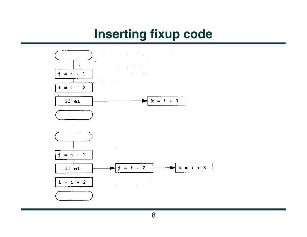
Inserting fixup code

9

Trace Scheduling •  Trace scheduling avoids moving operations above splits or below

joins unless it can prove that other instructions will not be adversely affected

•  Trace scheduling will always converge •  However, in the worst case, a very large amount of fixup code

may result — Worst case: operations increase to O(n en)

10

Straight-line Scheduling: Conclusion •  Issues in straight-line scheduling:

— Relative order of register allocation and instruction scheduling — Dealing with loads and stores: Without sophisticated analysis,

almost no movement is possible among memory references

11

Kernel Scheduling •  Drawback of straight-line scheduling:

— Loops are unrolled. — Ignores parallelism among loop iterations

•  Kernel scheduling: Try to maximize parallelism across loop iterations

12

Kernel Scheduling •  Schedule a loop in three parts:

— a kernel: includes code that must be executed on every cycle of the loop

— a prolog: which includes code that must be performed before steady state can be reached

— an epilog, which contains code that must be executed to finish the loop once the kernel can no longer be executed

•  The kernel scheduling problem seeks to find a minimal-length kernel for a given loop

•  Issue: loops with small iteration counts?

13

Kernel Scheduling: Software Pipelining •  A kernel scheduling problem is a graph:

G = (N, E, delay, type, cross) where cross (n1, n2) defined for each edge in E is the number of iterations crossed by the dependence relating n1 and n2 — Dependence distance

•  Temporal movement of instructions through loop iterations •  Software Pipelining: Body of one loop iteration is pipelined

across multiple iterations.

14

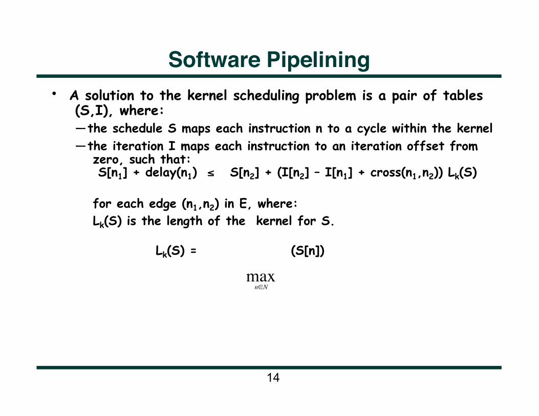
Software Pipelining •  A solution to the kernel scheduling problem is a pair of tables

(S,I), where: — the schedule S maps each instruction n to a cycle within the kernel — the iteration I maps each instruction to an iteration offset from

zero, such that: S[n1] + delay(n1) ≤ S[n2] + (I[n2] – I[n1] + cross(n1,n2)) Lk(S)

for each edge (n1,n2) in E, where: Lk(S) is the length of the kernel for S.

Lk(S) = (S[n])

n∈Nmax

15

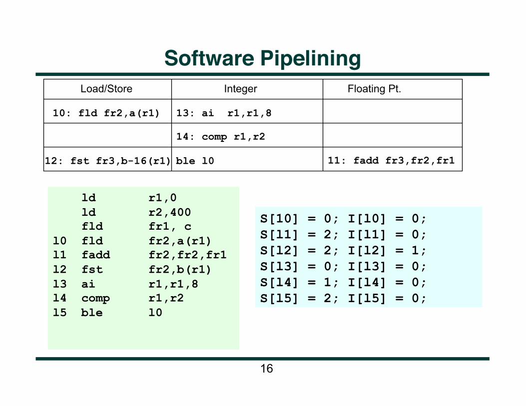
Software Pipelining •  Example: ld r1,0

ld r2,400 fld fr1, c l0 fld fr2,a(r1) l1 fadd fr2,fr2,fr1

l2 fst fr2,b(r1) l3 ai r1,r1,8 l4 comp r1,r2 l5 ble l0

•  A legal schedule:

10: fld fr2,a(r1) 13: ai r1,r1,8

Floating Pt.

14: comp r1,r2

12: fst fr3,b-16(r1) ble l0 11: fadd fr3,fr2,fr1

Integer Load/Store

16

Software Pipelining

ld r1,0 ld r2,400 fld fr1, c l0 fld fr2,a(r1) l1 fadd fr2,fr2,fr1 l2 fst fr2,b(r1) l3 ai r1,r1,8 l4 comp r1,r2 l5 ble l0

S[10] = 0; I[l0] = 0; S[l1] = 2; I[l1] = 0; S[l2] = 2; I[l2] = 1; S[l3] = 0; I[l3] = 0; S[l4] = 1; I[l4] = 0; S[l5] = 2; I[l5] = 0;

10: fld fr2,a(r1) 13: ai r1,r1,8

Floating Pt.

14: comp r1,r2

12: fst fr3,b-16(r1) ble l0 11: fadd fr3,fr2,fr1

Integer Load/Store

17

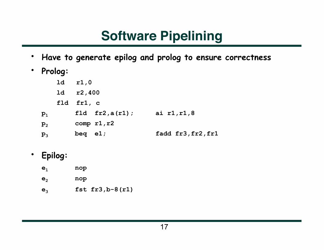
Software Pipelining •  Have to generate epilog and prolog to ensure correctness •  Prolog: ld r1,0

ld r2,400

fld fr1, c

p1 fld fr2,a(r1); ai r1,r1,8

p2 comp r1,r2

p3 beq e1; fadd fr3,fr2,fr1

•  Epilog: e1 nop

e2 nop

e3 fst fr3,b-8(r1)

18

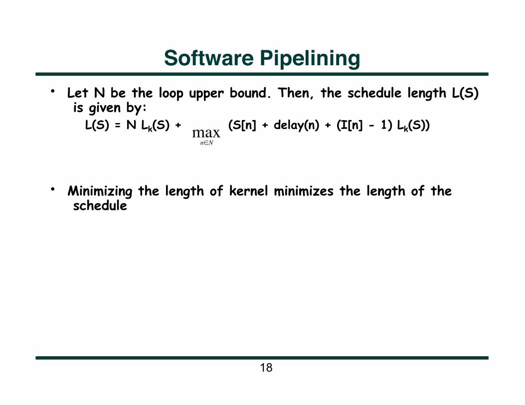
Software Pipelining •  Let N be the loop upper bound. Then, the schedule length L(S)

is given by: L(S) = N Lk(S) + (S[n] + delay(n) + (I[n] - 1) Lk(S))

•  Minimizing the length of kernel minimizes the length of the schedule

n∈Nmax

19

Kernel Scheduling Algorithm •  Is there an optimal kernel scheduling algorithm?

•  Try to establish lower bound on how well scheduling can do: how short can a kernel be? — Based on available resources — Based on data dependences

20

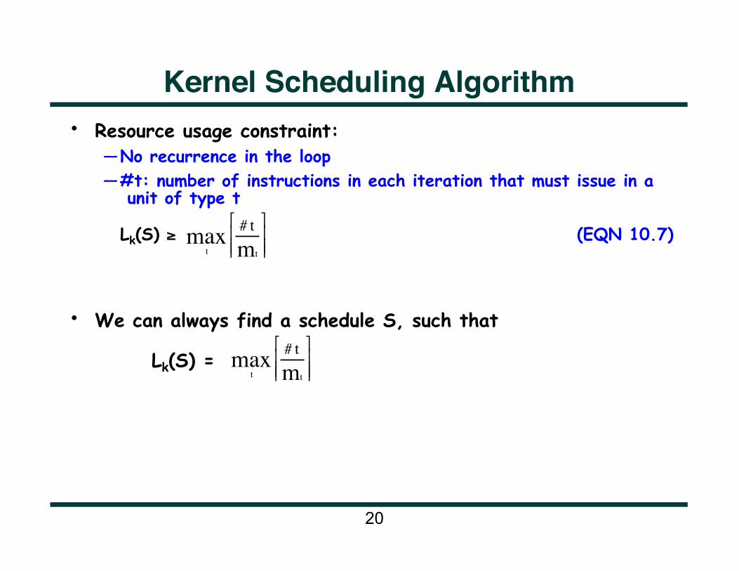
Kernel Scheduling Algorithm •  Resource usage constraint:

— No recurrence in the loop — #t: number of instructions in each iteration that must issue in a

unit of type t

Lk(S) ≥ (EQN 10.7)

•  We can always find a schedule S, such that

Lk(S) =

tmax # t

tm

tmax # t

tm

21

Software Pipelining Algorithm

l0 ld a,x(i)

l1 ai a,a,1

l2 ai a,a,1

l3 ai a,a,1

l4 st a,x(i)

Memory1 Integer1 Integer2 Integer3 Memory2

10: S=0; I=0 11: S=0; I=1 12: S=0; I=2 13: S=0; I=3 14: S=0; I=4

22

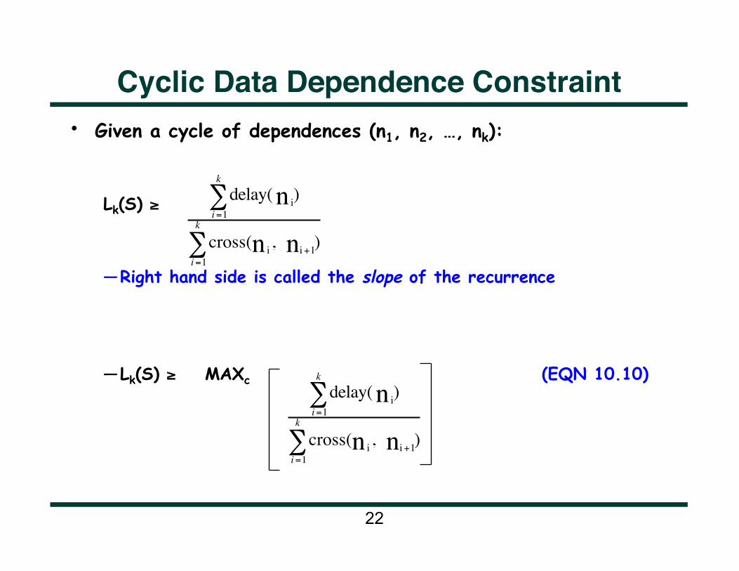
Cyclic Data Dependence Constraint •  Given a cycle of dependences (n1, n2, …, nk):

Lk(S) ≥

— Right hand side is called the slope of the recurrence

— Lk(S) ≥ MAXc (EQN 10.10)

delay( in )i=1

k

∑

cross( in , i+1 n )i=1

k

∑

delay( in )i=1

k

∑

cross( in , i+1 n )i=1

k

∑

23

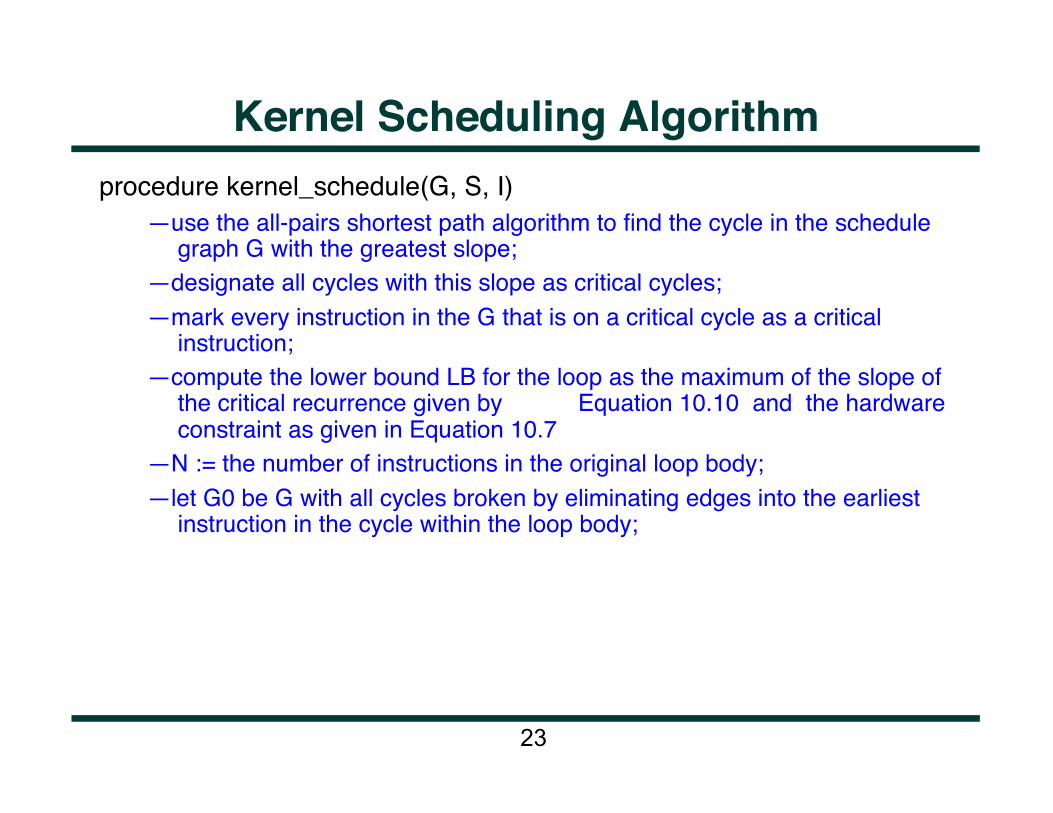
Kernel Scheduling Algorithm procedure kernel_schedule(G, S, I)

— use the all-pairs shortest path algorithm to find the cycle in the schedule graph G with the greatest slope;

— designate all cycles with this slope as critical cycles; — mark every instruction in the G that is on a critical cycle as a critical

instruction; — compute the lower bound LB for the loop as the maximum of the slope of

the critical recurrence given by Equation 10.10 and the hardware constraint as given in Equation 10.7

— N := the number of instructions in the original loop body; — let G0 be G with all cycles broken by eliminating edges into the earliest

instruction in the cycle within the loop body;

24

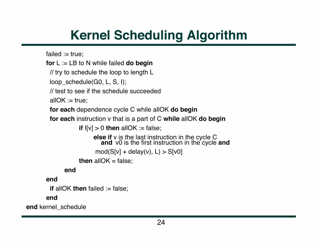
Kernel Scheduling Algorithm failed := true; for L := LB to N while failed do begin // try to schedule the loop to length L loop_schedule(G0, L, S, I); // test to see if the schedule succeeded allOK := true; for each dependence cycle C while allOK do begin for each instruction v that is a part of C while allOK do begin if I[v] > 0 then allOK := false; else if v is the last instruction in the cycle C and v0 is the first instruction in the cycle and mod(S[v] + delay(v), L) > S[v0] then allOK = false; end end if allOK then failed := false; end

end kernel_schedule

25

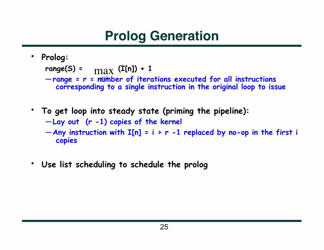
Prolog Generation •  Prolog:

range(S) = (I[n]) + 1 — range = r = number of iterations executed for all instructions

corresponding to a single instruction in the original loop to issue

•  To get loop into steady state (priming the pipeline): — Lay out (r -1) copies of the kernel — Any instruction with I[n] = i > r -1 replaced by no-op in the first i

copies

•  Use list scheduling to schedule the prolog

n∈Nmax

26

Epilog Generation •  After last iteration of kernel, r - 1 iterations are required to

wind down •  However, must also account for last instructions to complete to

ensure all hazards outside the loop are accommodated •  Additional time required:

ΔS = ( (( I[n] - 1)Lk(S) + S[n] + delay(n)) - rLk(S))+

•  Length of epilog: (r - 1) Lk(S) + ΔS

n∈Nmax

27

Software Pipelining: Conclusion •  Issues to consider in software pipelining:

— Increased register pressure: May have to resort to spills

•  Control flow within loops: — Use If-conversion or construct control dependences — Schedule control flow regions using a non-pipelining approach and

treat those areas as black boxes when pipelining

28

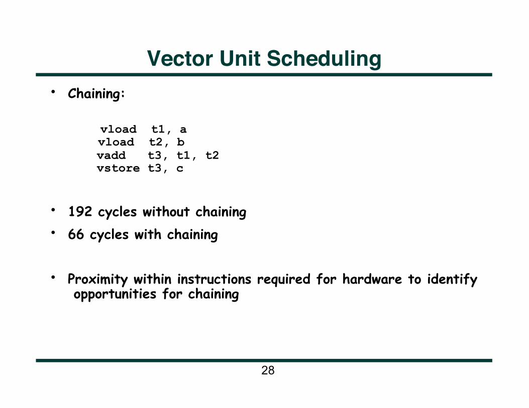
Vector Unit Scheduling •  Chaining:

vload t1, a vload t2, b

vadd t3, t1, t2 vstore t3, c

•  192 cycles without chaining •  66 cycles with chaining

•  Proximity within instructions required for hardware to identify opportunities for chaining

29

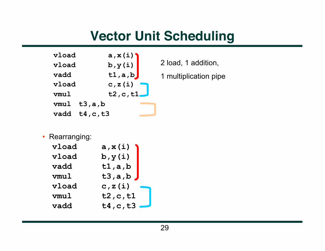
Vector Unit Scheduling vload a,x(i) vload b,y(i) vadd t1,a,b vload c,z(i) vmul t2,c,t1 vmul t3,a,b vadd t4,c,t3

•  Rearranging: vload a,x(i) vload b,y(i) vadd t1,a,b vmul t3,a,b vload c,z(i) vmul t2,c,t1 vadd t4,c,t3

2 load, 1 addition,

1 multiplication pipe

30

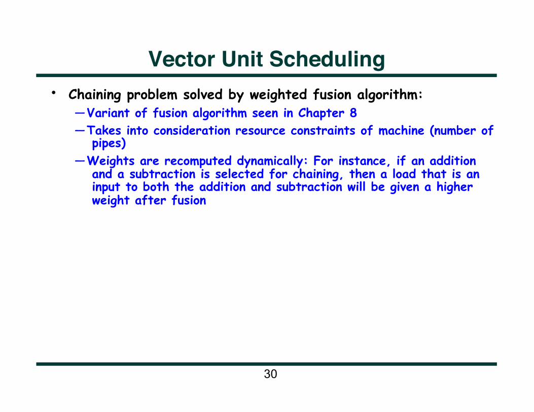
Vector Unit Scheduling •  Chaining problem solved by weighted fusion algorithm:

— Variant of fusion algorithm seen in Chapter 8 — Takes into consideration resource constraints of machine (number of

pipes) — Weights are recomputed dynamically: For instance, if an addition

and a subtraction is selected for chaining, then a load that is an input to both the addition and subtraction will be given a higher weight after fusion

31

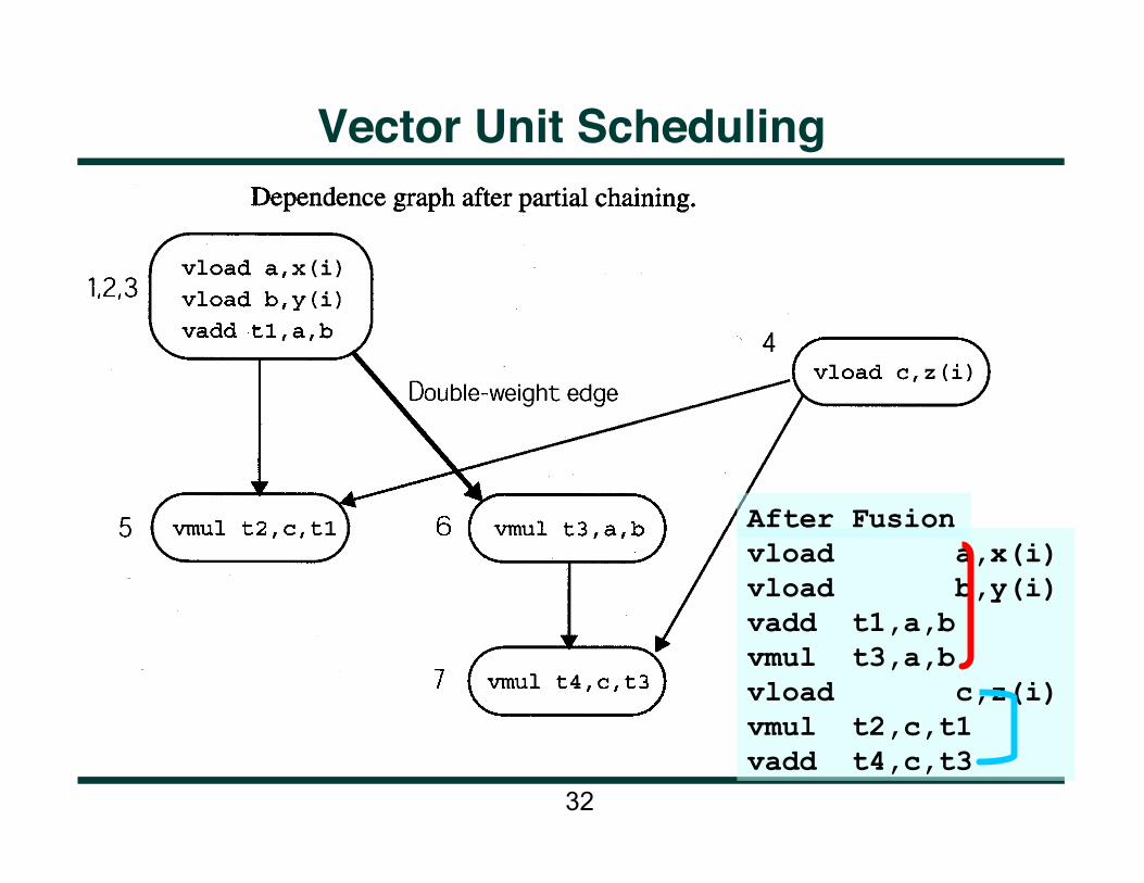
Vector Unit Scheduling

vload a,x(i) vload b,y(i) vadd t1,a,b vload c,z(i) vmul t2,c,t1 vmul t3,a,b vadd t4,c,t3

32

Vector Unit Scheduling

vload a,x(i) vload b,y(i) vadd t1,a,b vmul t3,a,b vload c,z(i) vmul t2,c,t1 vadd t4,c,t3

After Fusion

33

Co-processors •  Co-processor can access main memory,

but cannot see the cache •  Cache coherence problem •  Solutions:

— Special set of memory synchronization operations

— Stall processor on reads and writes (waits)

•  Minimal number of waits essential for fast execution

•  Use data dependence to insert these waits

•  Positioning of waits important to reduce number of waits

•  These techniques also apply to modern accelerators such as GPGPU’s

34

Co-processors •  Algorithm to insert waits:

— Make a single pass starting from the beginning of the block — Note source of edges — When target reached, insert wait

•  Produces minimum number of waits in absence of control flow

•  Minimizing waits in presence of control flow is NP Complete. Compiler must use heuristics

35

Conclusion •  We looked at:

— Straight line scheduling: For basic blocks — Trace Scheduling: Across basic blocks — Kernel Scheduling: Exploit parallelism across loop iterations — Vector Unit Scheduling — Issues in cache coherence for coprocessors