Community Detection applied to Cross-Device Identity Graphs

IN DEGREE PROJECT COMPUTER SCIENCE AND ENGINEERING,SECOND CYCLE, 30 CREDITS

, STOCKHOLM SWEDEN 2017

Community Detection applied to Cross-Device Identity Graphs

VALENTIN GEFFRIER

KTH ROYAL INSTITUTE OF TECHNOLOGYSCHOOL OF COMPUTER SCIENCE AND COMMUNICATION

Abstract

The personalization of online advertising has now become a necessity for mar-keting agencies. The tracking technologies such as third-party cookies givesadvertisers the ability to recognize internet users across different websites, to un-derstand their behavior and to assess their needs and their tastes. The amountof created data and interactions leads to the creation of a large cross-deviceidentity graph that links different identifiers such as emails to different devicesused on different networks. Over time, strongly connected components appearin this graph, too large to represent only the identifiers or devices of only oneperson or household. The aims of this project is to partition these componentsaccording to the structure of the graph and the features associated to the edgeswithout separating identifiers used by a same person. Subsequent to this, thesize reduction of these components leads to the isolation of individuals and theidentifiers associated to them. This thesis presents the design of a bipartitegraph from the available data, the implementation of different community de-tection graphs adapted to this specific case and different validation methodsdesigned to assess the quality of our partition. Different graph metrics are thenused to compare the outputs of the algorithms and we will observe how theadaptation of the algorithm to the bipartite case can lead to better results.

Anpassningen av onlineannonsering har nu blivit en nödvändighet för mark-nadsföringsbyråer. Spårningstekniken som cookies från tredje part ger annon-sörer möjlighet att känna igen internetanvändare på olika webbplatser, för attförstå deras beteende och för att bedöma deras behov och deras smak. Mängdenskapade data och interaktioner leder till skapandet av en stor identitetsgrafik förflera enheter som länkar olika identifierare, t.ex. e-postmeddelanden till olikaenheter som används i olika nätverk. Över tiden visas starkt anslutna kompo-nenter i det här diagrammet, för stora för att endast representera identifierareeller enheter av endast en person eller hushåll. Syftet med detta projekt är attpartitionera dessa komponenter enligt grafens struktur och de egenskaper som ärknutna till kanterna utan att separera identifierare som används av samma per-son. Efter detta leder storleksreduktionen av dessa komponenter till isoleringenav individer och de identifierare som är associerade med dem. Denna avhandlingpresenterar utformningen av en bifogad graf från tillgängliga data, genomföran-det av olika samhällsdetekteringskurvor anpassade till detta specifika fall ocholika valideringsmetoder som är utformade för att bedöma kvaliteten på vårpartition. Olika grafvärden används då för att jämföra algoritmens utgångaroch vi kommer att observera hur anpassningen av algoritmen till tvåpartsfalletkan leda till bättre resultat.

Acknowledgements

I would like first to thank 1000mercis, the company which hosted me for thisproject, who gave me the means and the support I needed. Then the differentsupervisors who helped me during this project.

Pierre Colin and Romain Tailhades both data scientists at 1000mercis fortheir advices and ideas.

Erik Fransén my supervisor at KTH for his availability and his machinelearning knowledge.

Johan Håstad for accepting to examine my thesis.

Thanks also to the rest of the datascience team of 1000mercis for helpingme and creating a perfectly studious atmosphere.

Contents

1 Introduction 31.1 Context . . . . . . . . . . . . . . . . . . . . . . . . . . . . . . . . 31.2 Aim and Scope . . . . . . . . . . . . . . . . . . . . . . . . . . . . 41.3 Ethical Considerations . . . . . . . . . . . . . . . . . . . . . . . . 51.4 Limitations . . . . . . . . . . . . . . . . . . . . . . . . . . . . . . 6

2 Graph clustering 72.1 Graph theory . . . . . . . . . . . . . . . . . . . . . . . . . . . . . 72.2 Community structure . . . . . . . . . . . . . . . . . . . . . . . . 82.3 Algorithms validation, metrics and partition distance . . . . . . . 8

2.3.1 Modularity . . . . . . . . . . . . . . . . . . . . . . . . . . 82.3.2 Bipartite modularity . . . . . . . . . . . . . . . . . . . . . 92.3.3 Local Modularity . . . . . . . . . . . . . . . . . . . . . . . 92.3.4 The resolution parameter . . . . . . . . . . . . . . . . . . 102.3.5 Partition distances . . . . . . . . . . . . . . . . . . . . . . 102.3.6 Rewiring . . . . . . . . . . . . . . . . . . . . . . . . . . . 122.3.7 Without a golden-truth partition . . . . . . . . . . . . . . 12

3 Unsupervised learning and clustering 133.1 Clustering algorithms . . . . . . . . . . . . . . . . . . . . . . . . 133.2 Graph Clustering algorithms . . . . . . . . . . . . . . . . . . . . 143.3 Algorithms in the scope of the project . . . . . . . . . . . . . . . 14

3.3.1 The Louvain Algorithm . . . . . . . . . . . . . . . . . . . 143.3.2 Bipartite Louvain . . . . . . . . . . . . . . . . . . . . . . . 163.3.3 Local Modularity optimization . . . . . . . . . . . . . . . 173.3.4 Infomap . . . . . . . . . . . . . . . . . . . . . . . . . . . . 173.3.5 Markov Clustering Algorithm (MCL) . . . . . . . . . . . . 193.3.6 A sparse version of MCL . . . . . . . . . . . . . . . . . . 203.3.7 Comparison on the karate club graph . . . . . . . . . . . 20

4 Results 224.1 Studied graph . . . . . . . . . . . . . . . . . . . . . . . . . . . . . 224.2 Performances of the Sparse MCL . . . . . . . . . . . . . . . . . . 23

4.2.1 Influence of the inflation factor . . . . . . . . . . . . . . . 23

1

CONTENTS 2

4.3 Measures of modularity . . . . . . . . . . . . . . . . . . . . . . . 244.3.1 Influence of the resolution parameter . . . . . . . . . . . . 25

4.4 Validation . . . . . . . . . . . . . . . . . . . . . . . . . . . . . . . 274.4.1 Partition distance . . . . . . . . . . . . . . . . . . . . . . 274.4.2 IP addresses . . . . . . . . . . . . . . . . . . . . . . . . . 284.4.3 Lifetime of the inter-cluster-edges . . . . . . . . . . . . . . 31

4.5 Time . . . . . . . . . . . . . . . . . . . . . . . . . . . . . . . . . . 324.6 Synthesis . . . . . . . . . . . . . . . . . . . . . . . . . . . . . . . 33

5 Conclusion 34Bibliography . . . . . . . . . . . . . . . . . . . . . . . . . . . . . . . . 38

Chapter 1

Introduction

1.1 Context1000mercis is a French digital marketing company which provides Customer Re-lationship Management (CRM) services and online advertising to a wide panelof clients from different sectors, such as bank, insurance, Consumer PackageGoods brands, NGO,... They allow their clients to target specific groups ofpeople on various channels: emails, online display, texts. This has been madepossible by the use of cookies which are small text files stored on web browser,containing one id unique for each browser of each device. They can be createdwhen a user is exposed to one the marketing campaigns, opens one of the emailsor visits the website of one of the company’s clients. The performances of cam-paign can then be computed by counting the proportion of people who, afterhaving been exposed, purchased a product on the website of the client.

The cookies can then be used to target these specific people with tailoredads according to their customer journey. When the user cookie is observedwith an email address (for example after an email opening or a registrationon a website), the id of the cookie and a hash (for confidentiality reasons) ofthe email address are stored in a database along with the date and time ofthe observation, the IP address of the network and the type of device used bythe user. A graph is built with email addresses and cookies as nodes and theedges represent an observation of this email address on a browser containing thiscookie. This is very useful for companies that have database filled with emailaddresses of former customers they want to reach on a different channel. AsFacebook, Google, Amazon, Liveramp and a lot of other companies, 1000merciscan find the cookies linked to these addresses and target them specifically online.

To measure performances of marketing campaigns, most of the marketingagencies consider that a purchase on a client website can be attributed to theircampaign if at least one banner was shown to the buyer the week before. This

3

CHAPTER 1. INTRODUCTION 4

can maybe not measure the real effect of the campaign because this buyer couldhave made his purchase without advertising. That is why 1000mercis uses aA/B testing protocol to take into account the organic purchases of the web-site. One group of email addresses is exposed, another is not and at the end ofthe campaign, the increment of the banners exposition is measured as an upliftof the buying rate between both groups. This supposes that both groups arestatistically equal and completely independent. To ensure the latter condition,connected components of the graph are computed and groups A and B are builtwith email addresses and cookies belonging to the same connected componentsso that the intersection between groups A and B is empty.

This solution was acceptable as long the groups were statistically close, butafter several years of aggregating online data, components merged into one bigcomponent of millions and emails and dozens of millions of cookies. This hap-pened when devices were shared between different persons, the extreme examplebeing a library computer which can be linked to one cookie and hundreds of dif-ferent email addresses. This component can no longer be included in one groupor another without creating a bias, but removing it is a problem as it containsvery active cookies (very active because they belonged to devices linked directlyand indirectly to a lot of other devices), which would probably have been moreresponsive to a marketing campaign.

1.2 Aim and ScopeUsing connected components gave the same importance to every link betweennodes, and every link were kept in the analysis, which was a simple solutionwhen data was sparse. Now that the graph is more dense and connected, someedges need to be ignored. This can be done by applying community detectionalgorithms on the graph. Furthermore, these algorithms can refine the non-problematic components we had before, in order to keep only trustworthy edgesand be able to identify more clearly the cookies and the email addresses refer-ring to only one person. This would lead to a better understanding of how theseclusters form and how they interact.

Here, the original graph contains almost billions of nodes edges but dueto technical limitations, the different algorithms are applied on a subgraph of100,000 nodes and 120,000 edges here.

The goal of this thesis is to study, in the wide range of graph clusteringmethods, those who would be fit for our goal: for the type of clusters we arelooking for, on large-sized graphs, taking into account the bipartite property ofour graph if possible. In one specific case, we adapt a generic graph clusteringalgorithm in order to optimize a specific bipartite graph metric. We also adaptanother algorithm for large sparse graphs with a more relevant data structure.


After obtaining different partitions as outputs of this graph, we will need toolssuch as graph metrics, partition distances and others to evaluate these parti-tions which can be incomplete in the case of unsupervised learning as ours. Wewill also use the other data available that was not used by the algorithms. Theresults of this comparison will then be presented at the end of the thesis.

1.3 Ethical ConsiderationsWith the emergence of big data, marketers realized what this amount of datacould represent for the understanding of their customers’ behaviour, becausethey could now recognize people on the Internet and target them specifically.In order to protect the confidentiality of the users personal data, rules have beendesigned and ensure that these data are not kept more than a certain amount oftime by companies, only if they are truly needed and if the user gave his consentto this use of their data.

Furthermore, in order to keep tracks of a user without being able to asso-ciate him to a real person, only the hash of email addresses can be stored. Thishash, if it is done with an algorithm complex enough such as SHA-256, en-sures that today’s computers can not trace back an email address from its hash.Even if two strings are really close, their hashes can be completely different.This allows to have data that, if found by a another person, can not be associ-ated to a person. It is also strictly forbidden for someone who has access to thedata to hash an email address and see if it matches some records of the database.

If this data was to fall into the wrong hands, knowing more specific informa-tion about specific people could, with tedious work, lead to a de-anonymizationof the data[1]. This is why the anonymization of data can not be the onlysafeguard before sharing or selling it. As there are still grey areas on the legalaspects, marketing companies should be aware of these limitations and protectmore their user’s data even if they are not shared to others and even if the lawcan sometimes still be lenient about it.

The goal of this kind of data analysis is to group different hashed ids thatwould represent one person in order to consolidate the data and understand bet-ter which ads would be interesting for them. It can be seen as removing a noisefrom observations of different events without looking for the true identity of theusers and therefore remain within the law. This consolidation of the cookiesand email addresses will be used only in the company for analysis purposes andwill be not be shared or sold to other companies.


1.4 LimitationsIn order to use different machine learning libraries, we use Python to implementthe different algorithms and produce these results. Even though this languagecan be less quick than others, we think it is fitter for this kind of study whichaims at choosing one method among a wide panel. After this choice, it canbe interesting to use a different language like C++ to speed up an algorithmor languages such as Scala or Spark that enable distributed computations. Fortechnical reasons, the use of the cluster of the company was not possible duringthis project so we first manage to reduce the size of the graph in order to beable to test different algorithms on a laptop with 16Go of RAM and a processorIntel Core i7-7500U CPU with a 2.70GHz frequency, 2 cores and 4 threads.

Chapter 2

Graph clustering

2.1 Graph theoryA graph is a data structure that is particularly useful to describe links betweendifferent elements. The elements are called nodes or vertices and the links aredescribed by edges, which can be directed. In this thesis, because of the natureof the graph, we will focus on the case of undirected graphs. If the links donot have the same strength, weights can be associated to them and the graph isthen said to be weighted. We can use the notation G “ pW,V,Eq to designatethe graph G where V refers to the set of vertices of the graph, E the set of edgesof the graph and W the set of weights associated to each edge. For all pair ofnodes pna, nbq P V 2, if pna, nbq P E, then wa,b denotes the weight associated tohis edge. If the graph is unweighted, we will consider that all weights equal to 1.

For a node a, the degree is defined as the number of edges linked to a in thecase of an unweighted graph, or the sum of the weights associated to these edgesotherwise. Let n be the number of nodes, m half of the sum of the degrees ofthe nodes, which is the number of edges in the case of an unweighted graph.

A graph is bipartite if the set of nodes can be divided into two subsets suchthat all edges of the graph link one node from one subset to one of the other. Aswe will see later, our graph is bipartite as the edges represent the simultaneousobservation of an email address with a cookie id. The cookie ids will be onesubset and the email addresses another one.

The graph can also be represented by its adjacency matrix A with @pni, njq PV 2, Ai,j “ wi,j if pni, njq P E else 0. In the case of an undirected graph, thismatrix is symmetric, and if the graph is also bipartite, we can keep only therows referring to nodes of one set, and columns referring to nodes of the otherset, as all other elements of the matrix will be 0. This representation is a basisfor several methods and metrics and its eigenvalues and eigenvectors can be

7

CHAPTER 2. GRAPH CLUSTERING 8

interpreted as important indicators on the graph structure.

The output of our algorithms is a clustering of the graph, defined as apartition π of V the set of nodes: π “ pV1, ..., VKq,K ą 0,K ď |V |,YK

i“1Vi “ Vand if i ‰ j, Vi X Vj “ 0.

2.2 Community structureWhat these algorithms see as communities in these graphs are more denselyconnected groups of nodes, where the structure of the subgraph can be quitedifferent from the global graph. These communities should also be quite isolatedfrom each other. For example, in a people-based graph, a family or a group offriends will be represented by a dense part of the graph where most nodes arelinked with an edge because they have interactions with most of the other nodesof the group, whereas they will be less connected to the rest of the graph, ornot with the same people.

This is why community detection is part of unsupervised learning when wedo not have labels on the nodes. As other clustering problems, we need to groupsimilar points that are different from the other points, without a ground-truthpartition. This task is also more difficult when, as in our case, we have a largegraph which should be clustered in small communities containing cookies andemail addresses belonging to only one user, because we do not know the numberof clusters the partition should contain.

In most cases, the problem of finding the partition according to a certaincriterion is NP-hard, and if the complexity of a clustering algorithm is onlyquadratic, its performances can be quite disappointing.

2.3 Algorithms validation, metrics and partitiondistance

To measure the quality of a clustering, several papers have defined tools to ex-press mathematically the idea of community and assess the quality of partitionsgiven by the different algorithms.

2.3.1 ModularityOne of the most famous clustering measure is the modularity, designed by New-man [2], which has been used for more than a decade to compare most of thegraph clustering methods. It is defined as the ratio of edges within communitiesminus its expected value in a random graph where the nodes have the same de-gree as before and the rest is uniformly random, which is the null model. With


our notations:

Q “ 1{2mÿ

i,jPV

pAij ´ kikj{2mqδpCpiq, Cpjqq

Where Cpiq is the cluster containing the node i. It can also be reformulated likethis:

Q “Cÿ

c“1

pec ´ a2cq

where ec is the fraction of edges of the global graph with both ends in thecommunity c whereas ac is the fraction of edges of the global graph with atleast one end in community c. It was defined to be equal to zero in the caseof the null model. It takes values between -1 and 1 but starting from 0.3, thepartition is often considered as relevant which means that there is indeed acommunity structure in the graph and this structure is well represented by thispartition.

2.3.2 Bipartite modularityA variant of modularity has been defined for bipartite graphs by Barber[3] asthe null model can be more precise. Indeed, we know that some nodes can notbe linked together as they belong to the same type and so the expected numberof edges is different. We can then denote the bipartite modularity Qb as follows:

Qb “

Cÿ

c“1

pec ´ ac ˆ bcq

where ac is the fraction of edges of the global graph with the first type nodeend in community c and bc the fraction of edges of the global graph with thesecond type node end in community c.

2.3.3 Local ModularityWidely used, it has been demonstrated that modularity can miss small com-munities in large graph, or embedded in larger communities. Indeed, the as-sumption of the null model is that nodes can be linked to any other node inthe graph whereas in most of the real cases, nodes can only be linked to a localsmall part of the graph. If the network size increases, the expected number ofedges between two clusters decreases and can be less that one which can lead toan automatic merge of small clusters, even if they have a lot of internal edgesand just a few edges linking them because there will still be an increase of themodularity with the merging.

In order to solve this issue, Muff [4] have defined another metric, the localmodularity, similar to the modularity but for each community it only consid-ers the subgraph composed by the edges in the community and its neighbor


communities. This means it considers the ratio of edges inside the communityamong the edges in this subgraph and its expected value in the null model ofthis subgraph. This gives the same formula with:

Q “Cÿ

c“1

pec ´ a2cq

where ac and ec are, this time, the fraction of edges of the subgraph neighboringthe community c. This local version can also be adapted to the bipartite case.

2.3.4 The resolution parameterReichardt[5] introduced a Hamiltonian, generalized version of the modularitywith a resolution parameter r that allows to weigh the different terms of themodularity as follows:

Q “Cÿ

c“1

pr ˆ ec ´ a2cq

Where r is a real number greater than 0. When r is greater than 1, the modular-ity will have higher values with bigger clusters, and vice-versa. When r equals1, we have the original modularity. As we will see later, this parameter can beuseful for modularity optimization algorithm on large graphs as it allows to lookfor partitions with bigger or smaller clusters. Indeed, we might not want to findthe partition with the highest modularity among all possible partitions but onlyamong the partitions that have clusters with specific sizes, for example whenwe look for communities representing only one individual. It is proven that thisversion still has its limits [6].

2.3.5 Partition distancesFor some training graphs, one can have a golden-truth partition which representsthe true underlying partition of the graph. In order to compare the output ofan algorithm on this graph to the real partition, several indexes can be used [7]:

The Rand Index

This index introduced by Rand[8] counts the number of agreements from onepartition to another on each pair of nodes and divide it by the total number ofpairs of nodes. By agreement, we mean that in both partitions X and Y , thenodes a and b are in the same cluster or that in both partitions X and Y , thenodes a and b are in different clusters.

If we note t the number of pairs of nodes that are in the same cluster in Xand in the same cluster in Y , u the number of pairs of nodes that are in differentclusters in X and in different clusters in Y and N the number of nodes, then:

R “t` u

NpN ´ 1q{2


This index takes values between 0 and 1 but one needs to know the value it takesin a random case for it to be relevant. That is why the ARI has been creatednext. As we will see in our case, when there are many clusters, it is easy tohave a Rand index close to one because for example, taking the partition whereall the nodes are separated gives a lot of agreements between the two partitionson nodes that are not together, whereas we should focus on the nodes that aretogether in one of the partitions because they are less frequent.

The ARI or Adjusted Rand Index

This index is the corrected version of the Rand index so that it yields a value of1 if both partitions are identical, and 0 in average over all possible partitions.This means it can take negative values. With X “ tX1, X2, ..., Xru and Y “

tY1, Y2, ..., Ysu, @i, j ni,j “ |Xi

Ş

Yj |, ai “ř

j ni,j and bj “ř

i ni,j it can bewritten as follows:

ARI “R´ Expected R

Max R´ Expected R

“

ř

i,j

ˆ

ni,j2

˙

´

”

ř

i

ˆ

ai2

˙

ř

j

ˆ

bj2

˙

ı

{

ˆ

n

2

˙

1

2

”

ř

i

ˆ

ai2

˙

`ř

j

ˆ

bj2

˙

ı

´

”

ř

i

ˆ

ai2

˙

ř

j

ˆ

bj2

˙

ı

{

ˆ

n

2

˙

This versions corrects the bias we exposed in the former section as a positivevalue of the adjusted index shows a higher similarity compared to the randomcase which was not the case before. Nonetheless, as this method counts numbersof pairs, there is a quadratic relationship between this metric and cluster sizeswhich will affect much more the index when the clusters’ size will vary.

The NMI or normalized mutual information

This index is linked to the information theory and should measure the informa-tion shared by two partitions X and Y , or what we can learn on Y , knowing X.

The Shannon entropy for a partition X is hpXq “ ´ř

xPX ppxqlogpppxqqwhere ppxq is the probability for a node to be labeled as a member of the com-munity x.

We can define the same way hpY q and hpX,Y q “ ´ř

xPX

ř

yPY ppx, yqlogpppx, yqqwhere ppx, yq is the probability for a node to be labeled as a member of the com-munity x in the partition X and a member of the community y in the partitionY .

Then the mutual information [9] is

MIpX,Y q “ hpXq ` hpY q ´ hpX,Y q “ÿ

xPX

ÿ

yPY

ppx, yqlogppx, yq

ppxqppyq


and its normalized version can be obtained as follows:

NMIpX,Y q “MIpX,Y qa

hpXqhpY q

NMI equals 0 when partitions contain no information about one another, 1when they contain perfect information about one another i.e they are identical.

2.3.6 RewiringIn order to be sure that a metric such as modularity has a certain value becauseof an underlying community structure that we have been able to detect and notbecause of wider characteristics such as its degree distribution, one can rewirethe graph [10] [11] by swapping the ends of two edges chosen randomly for alarge enough number of pair of edges. Then the same algorithms are appliedto this new graph and the modularity can be computed to check if its value issignificantly lower than the one we had on the original graph.

2.3.7 Without a golden-truth partitionIf there is no golden-truth partition available, it is still possible to use other datathat would not have been used for the clustering. For example, the authors of theLouvain algorithm [12], have used community detection algorithms on mobileusers graphs where each node is a user and an edge represents a call betweentwo users. In order to test their clustering, they measured the homogeneity ineach cluster of a feature that they had not used before: the language associatedto each user device. The language homogeneity in each cluster showed thatnodes in the same cluster were similar according to a criteria that had not beenused in the clustering. The limit of their method was that nodes from differentclusters can also be similar according to this criteria so the basic partitionwhere all nodes are separated in their own cluster is perfect according only tothis measure. Clustering is also about creating groups that are different to eachother. In our case, we will use the IP address and design a rule in order to assessthe quality of our partition.

Chapter 3

Unsupervised learning andclustering

Clustering is one of the most frequent problems of unsupervised learning. Su-pervised learning actually train models by giving them for each sample theobjective they should tend to. This job can seem easier as the algorithm isgiven the groups from which he should learn and can then understand the sim-ilarities of points inside a group and dissimilarities between groups. Here, wehave to form the groups as well, and cannot as easily validate our results.

3.1 Clustering algorithmsGeneral clustering methods that were designed for vectors in a multi-dimensionalspace cannot be directly applied to graphs. One possibility is to first define adistance between nodes such as the shortest path that respects the definitionof a distance. However this requires to use either the Floyd-Warshall algorithm[13] that runs in Op|V |3q or Djikstra’s algorithm for each node that would thenrun in Op|V ||E| ` |V |2log|V |q which is better in a sparse graph when |E| issignificantly smaller than |V |2. One method for large graphs uses “landmarknodes” to approximate the distance and obtain a linear complexity in the sizeof the graph [14]. From this distance matrix, one can already apply hierarchicalalgorithms such as complete, single and average linkage [15], or Ward’s method[16]. If one wants to use algorithms that need nodes to be represented by vectorssuch as K-means or Mixture Models, finding a multidimensional space where wecan place these nodes and respect the distance we found between nodes is notsimple and can need a lot of dimensions. One solution presented is to use thecolumns of the distance matrix as vectors but this means that we would stillhave as many dimensions as the number of nodes. K-medoids [17] is also anadaptation that can work with the distance matrix as the only input.

13

CHAPTER 3. UNSUPERVISED LEARNING AND CLUSTERING 14

3.2 Graph Clustering algorithmsIn order to address the specific graph partitioning problem, various algorithmshave been designed and a exhaustive survey has been provided by Fortunato[18]. Some are variants of the algorithms presented above: hierarchical cluster-ing that uses graph-based distances, spectral clustering that places the nodes inthe linear span of first eigenvectors of a similarity matrix of the nodes and thenuses the k-means algorithms. Divisive algorithms [19] delete the edges that havethe highest betweenness which is the number of pairs of nodes whose shortestpath joining them contains this edge, until it has separated the graph in thedesired number of clusters. These algorithms were not kept in the scope of thisstudy as their complexity was too high for the size of the graph and most ofthem required the number of clusters as an input parameter whereas it is un-known in our case and can take a wide range of values.

An important aspect of our graph is that it is bipartite. In that case, inorder to avoid an abnormal behaviour of an algorithm because of this speci-ficity, one can use the projection graph which considers only one type of nodesand create edges between them if they had a common neighbour in the originalgraph. This technique reduces the number of nodes but it can also increase thenumber of edges: one second-type node which was linked to 10 first-type nodeswill be replaced by edges between each pair of nodes among these ten, and thiswill give 45 edges. Furthermore, in our case, the data carried by edges in theoriginal graph can no longer be used after the projection.

To detect communities in the graph, we choose to focus on local approaches,algorithms that would build small clusters without requiring the number ofclusters as an input, and with an appropriate scalability on large graphs to beable to test different algorithms with different parameters more quickly.

3.3 Algorithms in the scope of the project

3.3.1 The Louvain AlgorithmAs modularity is widely used to evaluate partitions of graph, some algorithmsfocus on its optimization. The greedy-optimization algorithm will try everypossible partition of the graph and find the one with highest modularity. Thisbecomes quickly unfeasible when the number of nodes increases as the numberof partitions of a graph of size n is the n-th Bell number (for n=19, this numberis already 5,832,742,205,057).

The Louvain algorithm [12] aims at finding local optima of the modularityamong all of the possible partitions by starting from the partition where allnodes are separated and then apply a local moving heuristic that moves onenode to another group as long as these actions make the modularity increase.


When it does not increase anymore, a new graph is built where nodes are thecommunities of the former graph then the local moving heuristic is applied againon these new nodes. The algorithm alternates these two steps until there is nochange in the partition. The advantage of this method is that the modularitydoes not have to be recomputed entirely at each change, only the difference hasto and its computation is easier. Optimizing the modularity is NP - hard butthis heuristic actually quickens the optimization and gives quite good results.This algorithm can be seen as a modularity optimization in the partition spaceswhere community merging between neighbours and moving one node from com-munity to another are the only authorized moves. It runs in Opnlogpnqq.

The algorithm can be written as follows:

input:G: graphc: initial assignment of nodes to communities (in our case, we start with all thenodes in their own cluster, cÐ r1...NumberOfNodespGqsq

output:c: Final assignment of nodes to communities

// Apply the local moving heuristiccÐ LocalMovingHeuristicpG, cq

if NumberOfCommunitiespcq ď NumberOfNodespGq then

// Produce the reduced networkGreduced Ð ReducedNetworkpG, cqcreduced Ð r1...NumberOfNodespGreducedqs

// Recursively call the algorithmcreduced Ð LouvainAlgorithmpGreduced, creducedq

// Merge the commmunities with the partition of the reduced graphcold Ð cfor iÐ 1 to NumberOfCommunitiespcoldq docpcold “ iq Ð creducedpiq

end forend if

Even if there is no self-loop in the original graph, when a new reduced graphis built from the communities, a self loop is added to each new node with aweight equal to the sum of the weights of the edges inside the cluster (includ-ing self loops) associated to this node. Edges between two communities arereplaced by one edge between the two nodes representing these communities


with a weight equal to the sum of the weight of these edges.

The difference of modularity caused by the insertion of the node i in thecommunity c can then be computed with the following formula:

∆Q “

«

ř

in,c`ki,c

2m´

ˆ

ř

tot,c`ki

2m

˙2ff

´

«

ř

in,c

2m´

ˆ

ř

tot,c

2m

˙2

´

ˆ

ki2m

˙2ff

Here,ř

in,c is the sum of all the weights of the links from and to the commu-nity c,

ř

tot,c is the sum of all the weights of the links to nodes of the communityc. ki,self represents the number of self-loops for the node i and is equal to 0 inour case when we have not reduced the graph yet.

This algorithm can also be used with the resolution parameter r and theformula becomes:

∆Q “

«

r

ř

in,c`ki,c

2m´

ˆ

ř

tot,c`ki

2m

˙2ff

´

«

r

ř

in,c

2m`ki,self

2m´

ˆ

ř

tot,c

2m

˙2

´

ˆ

ki2m

˙2ff

Some variants have been designed in order to move more freely in the parti-tions space, test more partitions and reach higher modularity values: Rotta [20]introduced a multilevel refinement that, once the original algorithm has beenapplied, allowed recursively to come back to the previous graphs and applyagain the local moving heuristic at each level which gives another possible movein the partitions space that is moving one node from a community to another.

The SLM algorithm [21] adds a step where before working on the reducedgraph, the first step of the algorithm would first be applied on the nodes of eachcommunity alone as a subgraph to create sub-communities that would then bethe nodes of the reduced graph of the next step which would start already withthe communities as partition. Splitting the communities again is another movepossible to explore the partitions’ space. In the same paper, authors showedthat simple several iterations of the basic Louvain algorithm where the outputof each iteration is used as the input of the next iteration, can still increaseslightly the modularity of the final partition.

3.3.2 Bipartite LouvainThe Louvain algorithm can be adapted to the bipartite version of modularity.The heuristics stay exactly the same, and we adapt the modularity differencecomputation as we need to keep in mind for each community the total degreeof edges with both ends in the community, the total degree of edges with onlythe first-type end in the community and the total degree of edges with onlythe second-type end in the community. We find then the expression of thebipartite modularity difference when inserting a node that was alone in anothercommunity with the following formula:


∆Qb “

„

ř

in,c`2ki,c ` ki,self

2m´

ˆ

ř

tot,c,1`ki,1

2m

ř

tot,2,c`ki,2

2m

˙

´

„

ř

in,c

2m`ki,self

2m´

ˆ

ř

tot,c,1

2m

ř

tot,c,2

2m

˙

´

ˆ

2ki,12m

ki,22m

˙

Here, ki,1 represents the degree of i pointing to first-type nodes, ki,2 repre-sents the degree of i pointing to second-type nodes,

ř

tot,1,c andř

tot,2,c can beunderstood the same way. During the first phase, when the graph has not beenreduced yet, either ki,1 “ 0 or ki,2 “ 0 because our graph is bipartite. When wereduce the graph, we need to pay attention specifically to keep for each clusterwhich part of its degree has first type node in the community and/or a secondtype node in the community.

This algorithm can also be used with the resolution parameter r and itsformula is easily obtained as for the classic Louvain algorithm.

3.3.3 Local Modularity optimizationWe can also adapt the Louvain algorithm with the local version of modularity.However, it is more complex. Indeed, in the cases of the classic and bipartitemodularity, the contribution of each cluster to the modularity depends on thecluster and the rest of the graph as a whole, not on the neighbour clusters. Thismeans that merging two communities or separating them will only change thecontribution of these two communities.

For the local modularity, the contribution of each cluster depends on thesize of its local subgraph and so on the sizes of the neighbour clusters. Thismeans that if we merge two communities, this will change the contribution ofthese two clusters but also the contributions of all of their neighbours. Thisgoes against the advantages of the local moving heuristic: the variation of thelocal modularity for the merging of two communities can not be computed asquickly. This is why we will not study this case in this thesis.

3.3.4 InfomapInfomap [22] uses the local moving heuristic of the Louvain algorithm and canalso be upgraded with its variants, except it optimizes a different score. Thisscore is the map equation, inspired by the information theory, and answers tothe following problem: imagine a random walker on the graph walking fromnode to node. We want to assign codewords to each node so that this walkcan be written as a sequence of these codewords. The codebook gives the cor-respondence between nodes and codewords. In order to minimize the lengthof this message, we use the Huffman code [23] to have one number per nodewritten with its binary notation. The Huffman algorithm ensures that the code


is prefix-free which means one number is not the prefix of another one and themessage can have only one interpretation. As the morse code does, the Huff-man code gives lower numbers to frequently visited nodes in order to reduce thelength of your message.

We do not focus on one walk but on an average walk and the average mes-sage length needed per step. To compute this value, we need the probabilityfor each node, which is in the case of an undirected graph, the relative weight

of the edges linked to this node pl “ř

iPV wilř

i,jPV wi,j. Then, the Shannon’s source

coding theorem gives a lower bound to the average length, which is the entropyof the codeword variable X: hpXq “ ´

ř

iPV pilogppiq.

This method can be optimized further in the specific case of a graph, as code-words can precede and follow only a codewords subgroup. More specifically, wecan see that if we have an underlying community structure in our graph, it isunderstandable that a random walker will more probably stay in a communityat least for a few steps before leaving for another community. It would be thenbe more optimal to have a codebook specifically for this community with shortercodewords for each node, and a codeword for when the walker exits the commu-nity, and a codeword in a global codebook to specify in the message when thewalker enters the community so that the receiver of the message knows when itmust switch to this community codebook (an example showing the benefit fromthe additional codebooks, taken from the original paper, can be found in theappendix).

For one partition of the graph, we can now have one global codebook witha codeword for each community, and a module codebook for each communitywith a codeword for each node and the exit. All of these codebooks are Huff-man codes but one codeword can be present in each of these codebooks withoutcompromising the unicity of the interpretation of the message.

Finding the best communities can now be seen as finding the partition thatgives the minimum length of the average walk description, which is representedby the map equation:

LpP q “ qÑhpQq `ÿ

c

pöc hcpXcq

where hpQq is the frequency-weighted average length of codewords in the globalindex codebook, c is one of the community of the partition P , qÑ “

ř

c qÑc

the probability of switching communities with qÑc the probability to exit thecommunity c. hcpXcq is the frequency-weighted average length of codewords inthe codebook of community c. pö

c “ř

iPc pi ` qÑc the probability of using thecodebook c at each step. This map equation is also the average of the differentcodebooks average length of codewords weighted by their probability of use.


After simplifying the equation, we can write in our case:

LpP q “ pÑlogppÑq´2ÿ

c

pÑc logppÑc q´

ÿ

nPV

pnlogppnq`ÿ

c

ppÑc `pcqlogppÑc `pcq

This is the two-level version of Infomap. The multi-level version of Infomap[24] allows to create a hierarchy with more levels of module codebooks withthe same rules. This can lead to another decrease of the minimum descriptionlength.

3.3.5 Markov Clustering Algorithm (MCL)The Markov Clustering Algorithm [25] also uses the random walker concept todetect communities. The idea is that a random walker will more often stay indense communities, so we study the probability of a random walker startingfrom a node i to arrive at a node j in N steps when N tends to infinity. Inorder to do so, we take the matrix M “ A` I with A the adjacency matrix andI the identity matrix, which allows the random walker to stay on a node and, inthe bipartite case, allows the algorithm to converge. M is then made stochasticby normalizing the columns so that in each column j, the coefficient at the rowj is the probability to be at the node i at the next step. Then the algorithmhave two phases repeated at each iteration:

The expansion takes the matrix to the power two to double the number ofsteps that the walker already took. Then each columns are normalized again.

The inflation takes each coefficient to a certain power (2 usually) which iscalled inflation factor and then normalize again. This step tends to increasethe highest probabilities and decrease the lowest ones which can speed up thealgorithm. Changing the inflation factor can have an influence on clusters’ size:a high inflation factor will disadvantage walks far from the original step and thewalker will more probably stay closer to the departure node, the clusters willthen be smaller. A low inflation factor will inversely give bigger clusters.

The Markov properties ensure that the matrix will converge to a limit, anequilibrium state where nodes will be part of attractor systems or point to oneor several of these attractor systems. This means that in the limit matrix, foreach node the column associated i will have a non zero entry at row i if it isan attractor and maybe others non-entry zero if there are other attractors inthe same attractor system. If not, the node will point to at least one attractorwho will be identified with the non-zero entries of this node’s associated col-umn. Attractors from the same system and nodes pointing to them are groupedinto clusters. Some random perturbations can be added if some nodes point todifferent attractor systems.

In the classic implementation, the algorithm converges when some values gobelow the threshold value for a float (2.210´308 for Python) to be considered as


zero entries. This allows the only non value zero entry left in the column (whenthere is only one left) to become one after normalization.

The disadvantage of this method is that this matrix can take a lot of space(to N2) if the graph has only one connected component, its diameter is low andthe threshold value is also really low as the expansion will populate quickly thematrix with non-zero entries.

3.3.6 A sparse version of MCLThe graph we on is very sparse so even if it has only one connected component,the number of edges is not much higher than the number of nodes, which meansthan the ratio of non-zero entries in the adjacency matrix is close to 1{N . Oneefficient way to store the matrix used by the MCL algorithm is the CSC (com-pressed sparse column) matrix format. This format reads the matrix column bycolumn left-to-right, top-to-bottom and stores only the nnz nonzero entries ofthe original matrix and their positions with three arrays:

1. The values array val of size nnz that stores the values of the entries inthe order of reading.

2. The indices array rowind of size nnz that stores the row index of eachentry in the order of reading.

3. The column pointers array colptr of size N ` 1, with colptrr0s “ 0 andcolptrrjs ´ colptrrj ´ 1s is the number of nonzero entries in the column j,so colptrrjs is the number of elements in the j first rows of the matrix. Itis referred to as the column pointers array because colptrrj´ 1s is also theindex of the val array where the j-th column’s values start to appear.

This format is also used in a recent paper which presents a new distributedversion of the MCL [26]. As long as our matrix is sparse, the space requirementof 2nnz`N`1 stays better. Nonetheless, as said before, the expansion part canat some point fill our entire matrix. To solve this limit, we increase significantlythe zero-value threshold from the default python value, 10´308, to values closerto 10´15 so that smaller values can be pruned earlier.

3.3.7 Comparison on the karate club graphIn order to see how this sparse version of MCL performs, we can use it to detectthe communities of the Karate Club graph [27] and see if it differs from theoriginal version of the algorithm. This comparison is indeed not possible onour graph because the memory space needed to store the adjacency matrix andthen the matrices the algorithm creates exceed the technical limitation of thisproject. For an inflation factor of 2 and zero-thresholds varying from 10´30to 10´2, we find the exact same partition for this graph than with the original


version.

Table 3.3.1: Results of the Sparse MCLMCL Sparse MCL

Threshold p10´238q 10´1 10´2 10´3 10´6 10´7

Iterations 18 9 11 12 12 13Values stored 1156 850 1136 1140 1156 1156Time (ms) 3 13 15 15 16 18

Here, we can see on the chart that the sparse algorithm needs a few less it-erations before the convergence (from 9 to 13 instead of 18), and will also needless memory space as the original version stores the entire adjacency matrix(down to 850 instead of 1156). Much more time is needed on this graph withthe sparse version on the graph but as it is much smaller, it cannot be a proofthat it would also be the case on a bigger graph.

Chapter 4

Results

4.1 Studied graphThe graph we apply these algorithms on is a bipartite graph with cookie idsand email addresses, that have been attributed or observed by the company,each edge representing the observation of an email address on a client’s websitewith the id of the cookie the company put on the user’s browser. It is madeof billions of edges, hundreds of millions of emails and cookies. A first filter isapplied by removing cookies linked to more than 10 emails and emails linked to1000 cookies because they can be considered as outliers and so they are removedfrom the graph. This allows to ignore email addresses such as [email protected], orcookies of computers shared by many people, for example libraries’ computers.Then connected components of the graph are computed and this gives smallcomponents and one mega-component of million of emails, and still a few hun-dreds of millions of cookies and edges. Let us define the lifetime of an edgethe time between the first and the last simultaneous observation of the emailand the cookie linked by this edge. In order to keep only the skeleton of thiscomponent and because it is not possible anymore to consider that all edges canbe considered equally important, we remove all the edges that have a lifetimebelow 24 hours. This can be interpreted as saying: an email and a cookie arelinked only if this email has been used during more than one day on the browserthat contains the cookie. Then we keep only the biggest connected componentwhich is the most problematic one.

This final preprocessing gave one final connected component of 21,884 emails,80,787 cookies and only 122,206 edges which indicates that the graph is not verydensely connected anymore. Visualizations of this graph [28] with force orientedalgorithms to find position for the nodes that can reveal a community patterndo not give any insight or pattern. Other metrics can give a few more informa-tions on the graph. The maximum length of the shortest path between 2 nodesamong all pairs of nodes, i.e the diameter of the graph is 61 in this case. At

22

CHAPTER 4. RESULTS 23

some points, we can also wonder is the graph is made of some kind of chains,long sequences of nodes of degree 2 but most of these chains were not longerthan 3 edges. There is no nodes with very high degrees compared to the othersso the graph can be as a balanced network without clear patterns.

Nodes here carry almost no information. Cookies’ ids are generated ran-domly and email addresses are hashed with the MD5 algorithm for confidential-ity reasons. This algorithm is designed to make finding a string from its hashalmost impossible. Furthermore, with this method, two similar strings will havecompletely different hashes. This makes it impossible to use the domain of theemail addresses or to compute any distance between nodes’ names that wouldbe relevant.

However, edges carry a lot of informations. For each observation of this edge,we have its date and time, the IP address linked to the internet connection, thetype of browser and device. This can be used later for validation.

4.2 Performances of the Sparse MCLAfter comparing the MCL algorithm on the karate club graph, we can see herethe differences on our graph. The normal version of MCL can not be appliedhere because of the memory limit reached by the size of the adjacency matrix.However, the results of the sparse-MCL are much clearer now. Even if the num-ber of iterations does not decrease a lot with the threshold, we can see that forhigh thresholds, the algorithm is much quicker and needs less memory (as itstores only the non-zero values and their positions). Furthermore, in this casetoo, the partitions found with the different thresholds were identical, except forthresholds close to 1 such as 10´1 or 10´2.

Table 4.2.1: Influence of the threshold on the graph of concernThreshold 10´4 10´7 10´10 10´13 10´16

iterations 65 65 67 69 70Non zero values 1.2107 2.4107 1.5108 2.6108 3.0108

Time (ms) 27 51 150 351 512

In the following results, we will keep the threshold of 10´7 and change onlythe inflation factor.

4.2.1 Influence of the inflation factorOne way to obtain different results from the MCL algorithm is to change theinflation factor. Here are the different metrics and performances for inflationfactors from 1.2 to 6.


As expected, the number of clusters increase with the inflation factor, as therandom walker is pressured by the inflation to stay in a closer neighborhood.Then, we can see that the maximum number of non-zero values decrease a lotwhen the inflation factor increase as lower values get below the threshold morequickly. This means that the algorithm converges more quickly so the numberof iterations and the time needed also decrease.

We can even check that the average time by iteration decrease as the numberof values to process is lower with a high inflation factor. We see that we canhave a trade off between different metrics, according to the average size ofcommunities we want. Having a really low inflation factor would also meanthat we need to increase the zero-threshold if we have the same memory limitbecause the maximum number of non-zero-values can be much higher.

4.3 Measures of modularityWe can now compare the algorithms with different measures of modularity:


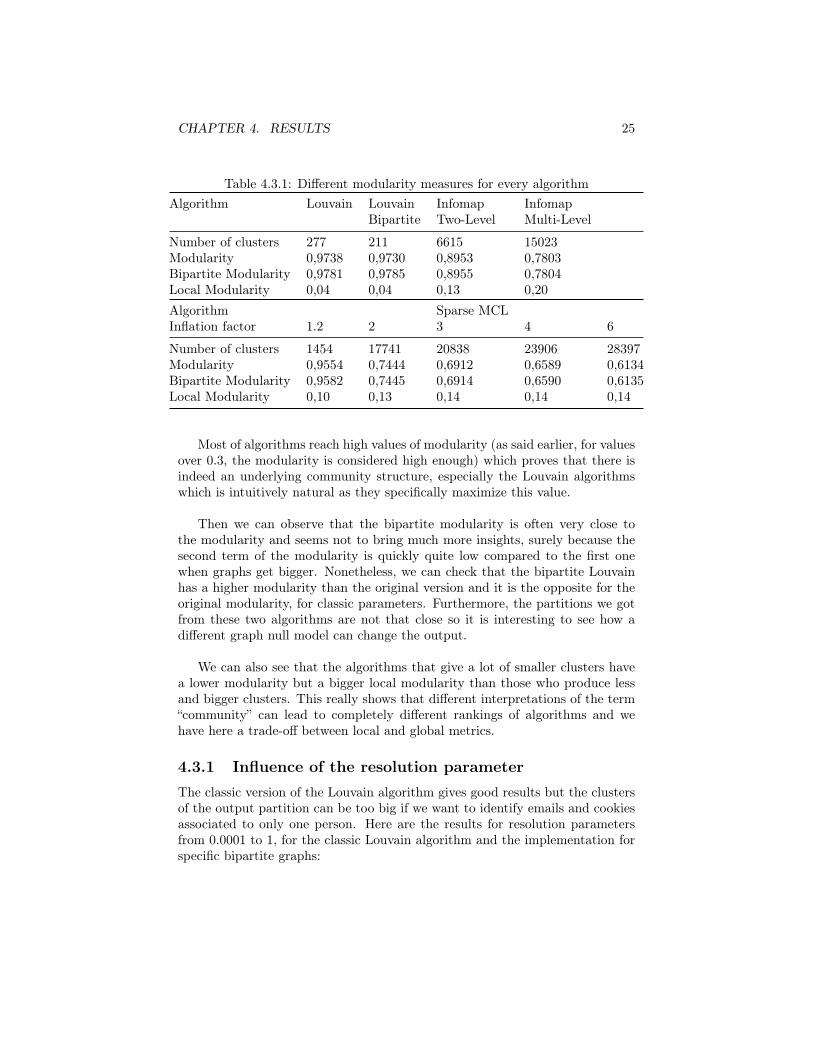
Table 4.3.1: Different modularity measures for every algorithmAlgorithm Louvain Louvain Infomap Infomap

Bipartite Two-Level Multi-Level

Number of clusters 277 211 6615 15023Modularity 0,9738 0,9730 0,8953 0,7803Bipartite Modularity 0,9781 0,9785 0,8955 0,7804Local Modularity 0,04 0,04 0,13 0,20Algorithm Sparse MCLInflation factor 1.2 2 3 4 6

Number of clusters 1454 17741 20838 23906 28397Modularity 0,9554 0,7444 0,6912 0,6589 0,6134Bipartite Modularity 0,9582 0,7445 0,6914 0,6590 0,6135Local Modularity 0,10 0,13 0,14 0,14 0,14

Most of algorithms reach high values of modularity (as said earlier, for valuesover 0.3, the modularity is considered high enough) which proves that there isindeed an underlying community structure, especially the Louvain algorithmswhich is intuitively natural as they specifically maximize this value.

Then we can observe that the bipartite modularity is often very close tothe modularity and seems not to bring much more insights, surely because thesecond term of the modularity is quickly quite low compared to the first onewhen graphs get bigger. Nonetheless, we can check that the bipartite Louvainhas a higher modularity than the original version and it is the opposite for theoriginal modularity, for classic parameters. Furthermore, the partitions we gotfrom these two algorithms are not that close so it is interesting to see how adifferent graph null model can change the output.

We can also see that the algorithms that give a lot of smaller clusters havea lower modularity but a bigger local modularity than those who produce lessand bigger clusters. This really shows that different interpretations of the term“community” can lead to completely different rankings of algorithms and wehave here a trade-off between local and global metrics.

4.3.1 Influence of the resolution parameterThe classic version of the Louvain algorithm gives good results but the clustersof the output partition can be too big if we want to identify emails and cookiesassociated to only one person. Here are the results for resolution parametersfrom 0.0001 to 1, for the classic Louvain algorithm and the implementation forspecific bipartite graphs:


The bipartite modularity is not shown as it was still almost equal to the clas-sic modularity. These values reveal that for smaller resolution parameters, theLouvain algorithm indeed finds smaller communities, but the bipartite imple-mentation which tries to optimize a different score actually gives partitions withhigher modularity values than the classic version, for example for a resolutionparameter of 0.0001, the modularity we get after applying the bipartite Louvainis 0.1 higher. This shows that knowing the graph is bipartite, the algorithmcan actually explore better partitions. Furthermore, even if the modularity andthe bipartite modularity are very close because it is computed on a large graph,when the local moving heuristic is applied, the difference between modularityand bipartite modularity variations will be more significant and it will lead todifferent clusters merging.

For low resolution parameters, we force the Louvain algorithm to optimizea score quite different from the classic modularity that is why the latter can bemuch lower (around 0.5 compared to the almost perfect modularity of 0.974 wehave in the classic case).


4.4 Validation

4.4.1 Partition distanceOne classic way to validate the algorithms is to use a ground truth partition,which would be the solution of our problems that help us validate the outputof an algorithm. In our case, we are able to find a partition for 4410 emailsof our graph. In another database, these emails are associated to names andzip codes. The partition is then defined by groups of emails linked to the samename and the same zip code. This data comes from clients files storing regularclients and these groups are much smaller because of the few interactions thereare, compared to our graph based on web navigations. We can then comparethe partition we had for these emails with the different algorithms to the groundtruth partition, with different indices.

Table 4.4.1: Partition distances to the ground-truth partitionAlgorithm Louvain Louvain Infomap Infomap


Number of clusters 277 211 6615 15023Rand index 0,98797 0,98464 0,99982 0,99994Adjusted Rand Score 0,004 0,003 0,201 0,369Normalized Mutual Information 0,020 0,019 0,134 0,287

Algorithm Sparse MCLInflation Factor 1.2 2 3 4 6

Number of clusters 1454 17741 20838 23906 28397Rand index 0,99090 0,99995 0,99996 0,99997 0,99997Adjusted Rand Score 0,005 0,344 0,266 0,199 0,146Normalized Mutual Information 0,031 0,310 0,268 0,170 0,106

As we can see in the charts, most of the algorithms have an excellent RandIndex (the maximum value being 1 for identical partitions), but it proves howthis index can be irrelevant without normalizing it. In our case, in the golden-truth partition, most of the pairs of emails belong to different clusters. In theoutputs of our algorithms too, but if we had a random algorithm creating verysmall clusters or even a partition where each node is alone in its cluster, wewould still have an index close to 1 as for most of pairs of emails, they aresupposed to be in different clusters.

NMI and ARI gives much more relevant value and take into account the scorethat we would have for random partitions, and weigh more the pair of nodesthat should be together as they are much more rare. The values are now muchlower but different enough to allow us to compare the algorithms. According


to this specific ground-truth partition, the multi-level version of the InfoMapalgorithm and the sparse MCL algorithm with an inflation factor of 2 seems toperform better than the others with respective ARI and NMI of 0.344 and 0.310for the space MCL, and 0.369 and 0.287 for the multi-level Infomap but we canalso check if we can have better results with different resolution parameters forthe Louvain Algorithm.

For the different resolution parameters, we have the following results:

We can see that for low resolution around 0.0005, the Louvain algorithmperforms almost as well because it gets NMI and ARI close to the values we hadfor the Sparse MCL and the multi-level Infomap, up to 0.3.

4.4.2 IP addressesAs our ground-truth partition is not exactly built on the same kind of inter-actions, we validate the results of other algorithms with different methods andwith the data that has not been used yet. The first other data available for eachedge is the different IP addresses for each edge. For each observation, the devicewhere the cookie is stored on accesses the Internet through a connection thatappears with a specific IP address. The device can be connected to differentnetworks so a cookie which is linked to only one device can be observed withdifferent IP addresses. For each edge, if the device linked to the cookie was not


mobile (because mobile can be linked to too many different IP shared by manymobiles using the same carrier in the same zone), we keep the most frequent IPaddress linked to this device and use the following hypothesis, described on thefigure.

If one email has been seen with different cookies but on the same IP, theyshould all three be in the same cluster. Why? Because it probably means thatthe cookies were either stored on the same device but not at the same time, orstored on different devices that used the same network of a household. On thecontrary, two different emails used on the same device and linked to the samecookie with the same address IP do not have to be in the same cluster as thissituation can occur if one uses a friend’s computer and enters an email addressdifferent than his friend’s.


Table 4.4.2: Performance according to the IP adresses ruleAlgorithm Louvain Louvain Infomap Infomap


Number of clusters 277 211 6615 15023Inter-cluster edges 2154 1955 12734 26815Invalid ones 328 304 3042 6488Ratio 15,2% 15,5% 23,9% 24,2%

Algorithm Sparse MCLInflation factor 1.2 2 3 4 6

Number of clusters 1454 17741 20838 23906 28397Inter-cluster edges 13381 31202 37702 41655 47226Invalid ones 2721 6810 8207 8712 9086Ratio 20,3% 21,8% 21,8% 20,9% 19,2%

In order to evaluate a partition, we count the proportion of inter-clusteredges that do not respect this rule. As we can see, the results are not signifi-cantly different, except for the Louvain algorithms that performs slightly better,and even more when the resolution parameter is closer to 0.005, with a ratiohigher than 25%. The limit of this validation is that it can be applied only on


edges linked to desktop devices whereas mobiles represent an important part ofthe devices in the graph.

Furthermore, the IP address of a network can change quite often so this datais not completely reliable. Finally, the value of this ratio should be computed inthe case of a random partition as the expected value of this ratio can probablyalso change depending on the number of clusters.

4.4.3 Lifetime of the inter-cluster-edgesTo overcome the last validation method limit, we use the average lifetime ofthe edges between the clusters, i.e the edges the algorithms considered as linksbetween communities that hase to be removed to view the underlying partitionbut also inside the cluster. The lifetime of each edge is the time between the firstand last observations of a cookie and an email together. The following figurecompares the average lifetime for inter-cluster edges and intra-cluster edges forthe different algorithms output.

Table 4.4.3: Average lifetime of the inter and intra-cluster edgesAlgorithm Louvain Louvain Infomap Infomap


Number of clusters 277 211 6615 15023Inter-cluster edges average lifetime 38,1 39 53,2 68,5Intra-cluster edges average lifetime 80,9 80,8 83,2 83,4


Number of clusters 1454 17741 20838 23906 28397Inter-cluster edges average lifetime 42,8 72,9 77 78,9 79,8Intra-cluster edges average lifetime 81,6 82,6 81,5 80,7 80,2

We can see here that the intra-cluster edges average lifetime is always higherthan the inter-cluster edges average lifetime. However, the difference is muchmore significant for the algorithms that gave less clusters, for example witha minimum value of 38.1 for the Inter-cluster edges average lifetime for theLouvain Algorithm. We can even see a pattern: when the number of clustersincreases, so does the average lifetime of the inter-cluster edges. An interpreta-tion is that the edges between the real communities have low lifetime becausethey occur less as anomalies do. The algorithms that create bigger communitieshave less edges to delete from the original graph in order to obtain the partition,and so they start with the less trustworthy one, which have low lifetimes. Onthe contrary, the ones which give small communities have more edges to cut toreach the final partition and if they approximately cut the edges by ascending


order of lifetime, the average can only be higher.

We can see that with lower values of the resolution parameter, we can getmuch better results as we still keep a low average edge lifetime for inter-clusteredges but a higher average edge lifetime value for the intra-cluster edges whichwas not the case for the other algorithms. This also validates the preprocessingwe did on the graph when we deleted edges with very low lifetimes.For exam-ple, for a resolution parameter of 5, we have 300 clusters and the intra-clusteredges average lifetime is 40 days much lower than the inter-cluster edges av-erage lifetime around 81, very close to the global average. On the opposite,for a resolution parameter of 0.0001 the intra-cluster edges average lifetime isaround 65 days but the inter-cluster edges average lifetime is between 95 and100 days, which is also significantly higher than the global average. This ten-dency confirms that this algorithm also cut edges following the ascending orderof the lifetime edges, when it gives more clusters, but even more than the othersalgorithms.

4.5 TimeMost of these algorithms were implemented with Python. The implementa-tion of Infomap available on http://www.mapequation.org [29] actually usesa wrapper and an implementation in C++. The running times are:

http://www.mapequation.org


Table 4.5.1: Running time of the different algorithmsAlgorithm Louvain Louvain Infomap Infomap


Time (seconds) 28 31 3 9


Time (seconds) 180 34 25 20 19

We can see that Infomap is running in less than 10 seconds so it is muchfaster thanks to the C++. The Louvain algorithm is also quite rapid, and theresolution parameter does not influence significantly the running time for ourrange of values.

4.6 SynthesisThis last validation method let us think that, in order to be cautious, for A/Btesting groups making, it is better to use the Louvain algorithms or the SparseMCL with an inflation factor of 1.2, that both seem to cut fewer but more rele-vant edges and give larger clusters because it is less likely to make mistakes andwe can afford large communities in this context. Louvain is quicker and has alinear memory complexity so it will scale better on larger graphs.

If we need to identify communities that represent individuals and thereforemust be much smaller, we would prefer the bipartite Louvain with a resolutionparameter between 0.001 and 0.005.

Chapter 5

Conclusion

The goal of this project is to find the best algorithms for different tasks on alarge people-based bipartite graph. In order to do so, we choose algorithms witha local approach but with different definitions of a community and different as-sumptions on the graph. We use the Infomap algorithm, the Louvain Algorithmthat are state of the art methods for this kind of objectives. Furthermore weadapt the Louvain algorithm to the specific case of our bipartite graph whichgives significantly better results. We also design a new version of the MarkovClustering algorithm (MCL) for sparse graphs with a fitter data structure whichallows to overcome the memory limit problem that this algorithm can quicklycreate when a graph begins to be too large.

To validate the outputs of the algorithms and compare their results, we usea wide set of indicators that can measure the quality of the partition on differentaspects: the density of the clusters and their interactions but also their closenessto a ground-truth partition. Leveraging the other data that is not used by thealgorithms, we are able to validate the performances of the new algorithms weimplement with an other approach.

Here some algorithms performs better on specific tasks so we can see howone is better for A/B testing groups division than for person-based clusters andvice-versa. This is also understable when observing the tradeoff we have be-tween different indices. This also prevents us from trusting only one indicatorto validate the results.

This work can be continued in many ways. First, a further and more thor-ough validation can be useful, if we had other data that can consolidate ourground-truth partition. A bipartite version of the Infomap algorithm where wecan add codebooks for each type of node in each community can optimize morethe map equation. Adapting Infomap for this kind of graph has partly beenexplored already [30].

34

CHAPTER 5. CONCLUSION 35

Other identifiers such as IDFA and AAID for mobiles can be inserted in thegraph as other node types because they are more reliable than cookies. Indeedthe cookies are not accepted by every user, and most users frequently deletetheir cookies which duplicate nodes and can alter the representation of the re-ality by the graph, the method from [31] can be implemented to overcome thisissue. Furthermore, the preprocessing of the graph to remove outliers can bedone with graph anomaly detection methods such as [32]. The IP address is nota reliable data but it can give information on the location of the networks andhelp for the validation as well.

Finally, a dynamic version of the algorithm can be useful as new nodes andedges appear every day and if the algorithm is going to be applied on the entiregraph, it will be more efficient to use the former outputs of the algorithm toinsert the new nodes in the existing communities or in new ones.

Bibliography

[1] Arvind Narayanan and Vitaly Shmatikov. Robust de-anonymization oflarge sparse datasets. In Security and Privacy, 2008. SP 2008. IEEE Sym-posium on, pages 111–125. IEEE, 2008.

[2] Mark EJ Newman and Michelle Girvan. Finding and evaluating communitystructure in networks. Physical review E, 69(2):026113, 2004.

[3] Michael J Barber. Modularity and community detection in bipartite net-works. Physical Review E, 76(6):066102, 2007.

[4] Stefanie Muff, Francesco Rao, and Amedeo Caflisch. Local modularitymeasure for network clusterizations. Physical Review E, 72(5):056107, 2005.

[5] Jörg Reichardt and Stefan Bornholdt. Detecting fuzzy community struc-tures in complex networks with a potts model. Physical Review Letters,93(21):218701, 2004.

[6] Andrea Lancichinetti and Santo Fortunato. Limits of modularity maxi-mization in community detection. Physical review E, 84(6):066122, 2011.

[7] Lawrence Hubert and Phipps Arabie. Comparing partitions. Journal ofclassification, 2(1):193–218, 1985.

[8] William M Rand. Objective criteria for the evaluation of clustering meth-ods. Journal of the American Statistical association, 66(336):846–850, 1971.

[9] Thomas M Cover. Elements of information theory thomas m. cover, joy a.thomas copyright c© 1991 john wiley & sons, inc. print isbn 0-471-06259-6online isbn 0-471-20061-1. 1991.

[10] Sergei Maslov and Kim Sneppen. Specificity and stability in topology ofprotein networks. Science, 296(5569):910–913, 2002.

[11] Ravi Kannan, Prasad Tetali, and Santosh Vempala. Simple markov-chainalgorithms for generating bipartite graphs and tournaments. RandomStructures and Algorithms, 14(4):293–308, 1999.

36

BIBLIOGRAPHY 37

[12] Vincent D Blondel, Jean-Loup Guillaume, Renaud Lambiotte, and EtienneLefebvre. Fast unfolding of communities in large networks. Journal ofstatistical mechanics: theory and experiment, 2008(10):P10008, 2008.

[13] Robert W Floyd. Algorithm 97: shortest path. Communications of theACM, 5(6):345, 1962.

[14] Zichao Qi, Yanghua Xiao, Bin Shao, and Haixun Wang. Toward a dis-tance oracle for billion-node graphs. Proceedings of the VLDB Endowment,7(1):61–72, 2013.

[15] Fionn Murtagh. A survey of recent advances in hierarchical clusteringalgorithms. The Computer Journal, 26(4):354–359, 1983.

[16] Joe H Ward Jr. Hierarchical grouping to optimize an objective function.Journal of the American statistical association, 58(301):236–244, 1963.

[17] Leonard Kaufman and Peter Rousseeuw. Clustering by means of medoids.North-Holland, 1987.

[18] Santo Fortunato. Community detection in graphs. Physics reports,486(3):75–174, 2010.

[19] Santo Fortunato, Vito Latora, and Massimo Marchiori. Method to findcommunity structures based on information centrality. Physical review E,70(5):056104, 2004.

[20] Randolf Rotta and Andreas Noack. Multilevel local search algorithms formodularity clustering. Journal of Experimental Algorithmics (JEA), 16:2–3, 2011.

[21] Ludo Waltman and Nees Jan van Eck. A smart local moving algorithm forlarge-scale modularity-based community detection. The European PhysicalJournal B, 86(11):471, 2013.

[22] M Rosvall and CT Bergstrom. Maps of information flow reveal communitystructure in complex networks. Technical report, Technical report, 2007.

[23] David A Huffman. A method for the construction of minimum-redundancycodes. Proceedings of the IRE, 40(9):1098–1101, 1952.

[24] Martin Rosvall and Carl T Bergstrom. Multilevel compression of randomwalks on networks reveals hierarchical organization in large integrated sys-tems. PloS one, 6(4):e18209, 2011.

[25] Stijn Marinus Van Dongen. Graph clustering by flow simulation. PhDthesis, 2001.

[26] Luwei He, Lu Lu, and Qiang Wang. An optimal parallel implementationof markov clustering based on the coordination of cpu and gpu. Journal ofIntelligent & Fuzzy Systems, 32(5):3609–3617, 2017.

BIBLIOGRAPHY 38

[27] Wayne W Zachary. An information flow model for conflict and fission insmall groups. Journal of anthropological research, 33(4):452–473, 1977.

[28] Thomas MJ Fruchterman and Edward M Reingold. Graph drawing byforce-directed placement. Software: Practice and experience, 21(11):1129–1164, 1991.

[29] D. Edler and M. Rosvall. The mapequation software package, availableonline at http://www.mapequation.org.

[30] Masoumeh Kheirkhahzadeh, Andrea Lancichinetti, and Martin Rosvall. Ef-ficient community detection of network flows for varying markov times andbipartite networks. Physical Review E, 93(3):032309, 2016.

[31] Anirban Dasgupta, Maxim Gurevich, Liang Zhang, Belle Tseng, andAchint O Thomas. Overcoming browser cookie churn with clustering. InProceedings of the fifth ACM international conference on Web search anddata mining, pages 83–92. ACM, 2012.

[32] Leman Akoglu, Hanghang Tong, and Danai Koutra. Graph based anomalydetection and description: a survey. Data Mining and Knowledge Discov-ery, 29(3):626–688, 2015.

http://www.mapequation.org

BIBLIOGRAPHY 39

These

figures,t

aken

from

theInfomap

original

pape

r[22]r

epresentstheuseof

theHuff

man

code

tocompressthemessage

representing

thespecificwalkof

thefig

ureA.The

figureB

show

stheop

timal

codebo

okwitho

utcommun

itiesan

dthefig

ure

Cshow

sthemod

ulecodebo

okof

each

commun

itiesan

dbe

low

thegrap

h,first

thecode

foreach

commun

ityin

theglob

alcodebo

ok(for

exam

ple111to

sign

alsthat

weentertheredcommun

ity)

andthen

theexit

code

foreach

commun

ityin

its

mod

ulecodebo

ok(for

exam

ple0001

tosign

alsthat

weexit

theredcommun

ity).The

figureD

givestheglob

alcode

book

.We

canverify

that

thesefiv

ecodebo

oksareindeed

prefix-free

andthat

themessage

that

represents

thewalkis

quiteshorterwith

thesead

dition

alcodebo

oks.

www.kth.se

Community Detection applied to Cross-Device Identity Graphs

Documents