Communication Networks · 2014-03-19 · Iterative, asynchronous each local iteration caused by: –local link cost change –distance vector update message from neighbor Distributed

Communication Networks

Routing and Traffic Management

Manuel P. Ricardo

Faculdade de Engenharia da Universidade do Porto

Routing

Graph – Directed and Undirected

Tree

Trees T = (V,E)

» graph with no cycles

» number of edges |E| = |V |−1

» any two vertices of the tree are connected by exactly one path

A tree T is said to span a graph G = (V,E) (spanning tree) if

» T = (V,E′) and E′ ⊆ E

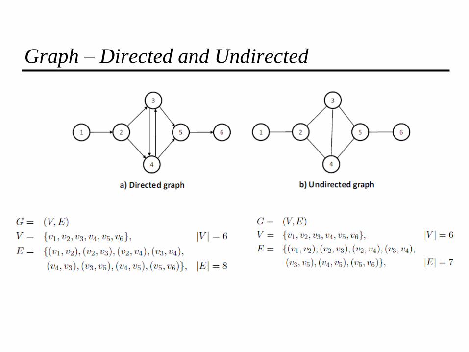
Shortest Path Trees

Graphs and Trees can be weighted » G=(V,E,w)

» T=(V, E’,w)

» w: ER

Total cost of a tree T

Minimum Spanning Tree T* » algorithms used to compute MST: Prism, Kruskal

Shortest Path Tree (SPT) Rooted at Vertex s » tree composed by the

» union of the shortest paths between s and each of other vertices of G

» Algorithms used to compute SPT: Dijkstra, Bellman-Ford

Computer networks use Shortest Path Trees

Routing in Datagram Networks

Forwarding, Routing

Forwarding data plane

» directing packet from input to output link

» using a forwarding table

Routing control plane

» computing paths the packets will follow

» routers exchanging messages

» each router creating its forwarding table

1

2 3

0111

destination

address

routing algorithm

local forwarding table

header value output link

0100

0101

0111

1001

3

2

2

1

Importance of Routing

End-to-end performance

» path affects quality of service

» delay, throughput, packet loss

Usage of network resources

» balance traffic over routers and links

» avoiding congestion by directing traffic to less-loaded links

Transient disruptions

» failures, maintenance

» limiting packet loss and delay during changes

Shortest-Path Routing

Path-selection model

» Destination-based

» Load-insensitive (e.g., static link weights)

» Minimum hop count or minimum sum of link weights

3

2

2

1

1

4

1

4

5

3

Shortest-Path Problem

Given a network topology with link costs

» c(x,y) - link cost from node x to node y

» Infinity - if x and y are not direct neighbors

Compute the least-cost paths from source u to all nodes p(v) - node predecessor of node v in the path to u

3

2

2

1

1

4

1

4

5

3

u

v

p(v)

Dijkstra’s Shortest-Path Algorithm

Iterative algorithm

» After k iterations known least-cost paths to k nodes

S set of nodes whose least-cost path is known

» Initially, S={u}, where u is the source node

» Add one node to S in each iteration

D(v) current cost of path from source to node v

» Initially

– D(v)=c(u,v) for all nodes v adjacent to u

– D(v)=∞ for all other nodes v

» Continually update D(v) when shorter paths are learned

Dijsktra’s Algorithm

1 Initialization:

2 S = {u}

3 for all nodes v

4 if v adjacent to u {

5 D(v) = c(u,v) }

6 else D(v) = ∞

7

8 Loop

9 find node w not in S with the smallest D(w)

10 add w to S

11 update D(v) for all v adjacent to w and not in S:

12 D(v) = min{D(v), D(w) + c(w,v)}

13 until all nodes in S

Dijkstra’s Algorithm - Example

3

2

2

1

1

4

1

4

5

3

3

2

2

1

1

4

1

4

5

3

3

2

2

1

1

4

1

4

5

3

3

2

2

1

1

4

1

4

5

3

Dijkstra’s Algorithm - Example

3

2

2

1

1

4

1

4

5

3

3

2

2

1

1

4

1

4

5

3

3

2

2

1

1

4

1

4

5

3

3

2

2

1

1

4

1

4

5

3

Shortest-Path Tree

Shortest-path tree from u Forwarding table at u

3

2

2

1

1

4

1

4

5

3

u

v

w

x

y

z

s

t

v (u,v)

w (u,w)

x (u,w)

y (u,v)

z (u,v)

link

s (u,w)

t (u,w)

Link-State Routing

Each router keeps track of its incident links

» link up, link down

» cost on the link

Each router broadcasts the link state

every router gets a complete view of the graph

Each router runs Dijkstra’s algorithm, to

» compute the shortest paths

» construct the forwarding table

Example protocols

» Open Shortest Path First (OSPF)

» Intermediate System – Intermediate System (IS-IS)

Detection of Topology Changes

Beacons generated by routers on links

» Periodic “hello” messages in both directions

» few missed “hellos” link failure

17

“hello”

Broadcasting the Link State

How to Flood the link state?

» every node sends link-state information

through adjacent links

» next nodes forward that info to all links

except the one where the information arrived

When to initiate flooding?

» Topology change

– link or node failure/recovery

– link cost change

» Periodically

– refresh link-state information

– typically 30 minutes

X A

C B D

(a)

X A

C B D

(b)

X A

C B D

(c)

X A

C B D

(d)

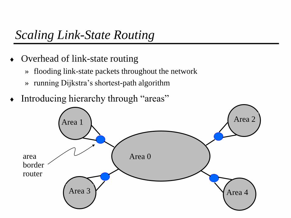
Scaling Link-State Routing

Overhead of link-state routing

» flooding link-state packets throughout the network

» running Dijkstra’s shortest-path algorithm

Introducing hierarchy through “areas”

Area 0

Area 1 Area 2

Area 3 Area 4

area border router

Bellman-Ford Algorithm

Define distances at each node x

» dx(y) = cost of least-cost path from x to y

Update distances based on neighbors

» dx(y) = min {c(x,v) + dv(y)} over all neighbors v

3

2

2

1

1

4

1

4

5

3

u

v

w

x

y

z

s

t du(z) = min{c(u,v) + dv(z), c(u,w) + dw(z)}

Distance Vector Algorithm

c(x,v) = cost for direct link from x to v

node x maintains costs of direct links c(x,v)

Dx(y) = estimate of least cost from x to y

node x maintains distance vector Dx = [Dx(y): y є N ]

Node x maintains also its neighbors’ distance vectors

for each neighbor v, x maintains Dv = [Dv(y): y є N ]

Each node v periodically sends Dv to its neighbors

» and neighbors update their own distance vectors

» Dx(y) ← minv{c(x,v) + Dv(y)} for each node y ∊ N

Over time, the distance vector Dx converges

Distance Vector Algorithm

Iterative, asynchronous

each local iteration caused by: – local link cost change

– distance vector update message from neighbor

Distributed

» node notifies neighbors only when its DV changes

Neighbors then

notify their neighbors,

if necessary

wait for (change in local link cost or

message from neighbor)

recompute estimates

if DV to any destination has

changed, notify neighbors

Each node:

Distance Vector Example - Step 0

A

E

F

C

D

B

2

3

6

4

1

1

1

3

Table for A

Dst Cst Hop

A 0 A

B 4 B

C –

D –

E 2 E

F 6 F

Table for B

Dst Cst Hop

A 4 A

B 0 B

C –

D 3 D

E –

F 1 F

Table for C

Dst Cst Hop

A –

B –

C 0 C

D 1 D

E –

F 1 F

Table for D

Dst Cst Hop

A –

B 3 B

C 1 C

D 0 D

E –

F –

Table for E

Dst Cst Hop

A 2 A

B –

C –

D –

E 0 E

F 3 F

Table for F

Dst Cst Hop

A 6 A

B 1 B

C 1 C

D –

E 3 E

F 0 F

Optimum 1-hop paths

Distance Vector Example - Step 1

Table for A

Dst Cst Hop

A 0 A

B 4 B

C 7 F

D 7 B

E 2 E

F 5 E

Table for B

Dst Cst Hop

A 4 A

B 0 B

C 2 F

D 3 D

E 4 F

F 1 F

Table for C

Dst Cst Hop

A 7 F

B 2 F

C 0 C

D 1 D

E 4 F

F 1 F

Table for D

Dst Cst Hop

A 7 B

B 3 B

C 1 C

D 0 D

E –

F 2 C

Table for E

Dst Cst Hop

A 2 A

B 4 F

C 4 F

D –

E 0 E

F 3 F

Table for F

Dst Cst Hop

A 5 B

B 1 B

C 1 C

D 2 C

E 3 E

F 0 F

Optimum 2-hop paths

A

E

F

C

D

B

2

3

6

4

1

1

1

3

Distance Vector Example - Step 2

Table for A

Dst Cst Hop

A 0 A

B 4 B

C 6 E

D 7 B

E 2 E

F 5 E

Table for B

Dst Cst Hop

A 4 A

B 0 B

C 2 F

D 3 D

E 4 F

F 1 F

Table for C

Dst Cst Hop

A 6 F

B 2 F

C 0 C

D 1 D

E 4 F

F 1 F

Table for D

Dst Cst Hop

A 7 B

B 3 B

C 1 C

D 0 D

E 5 C

F 2 C

Table for E

Dst Cst Hop

A 2 A

B 4 F

C 4 F

D 5 F

E 0 E

F 3 F

Table for F

Dst Cst Hop

A 5 B

B 1 B

C 1 C

D 2 C

E 3 E

F 0 F

Optimum 3-hop paths

A

E

F

C

D

B

2

3

6

4

1

1

1

3

Maximum Flow of a Network

Flow Network Model

Flow network

» source s

» sink t

» nodes a, b and c

Edges are labeled with capacities

» (e.g. bit/s)

Communication networks are not flow networks

» they are queue networks

» flow networks enable to determine limit values

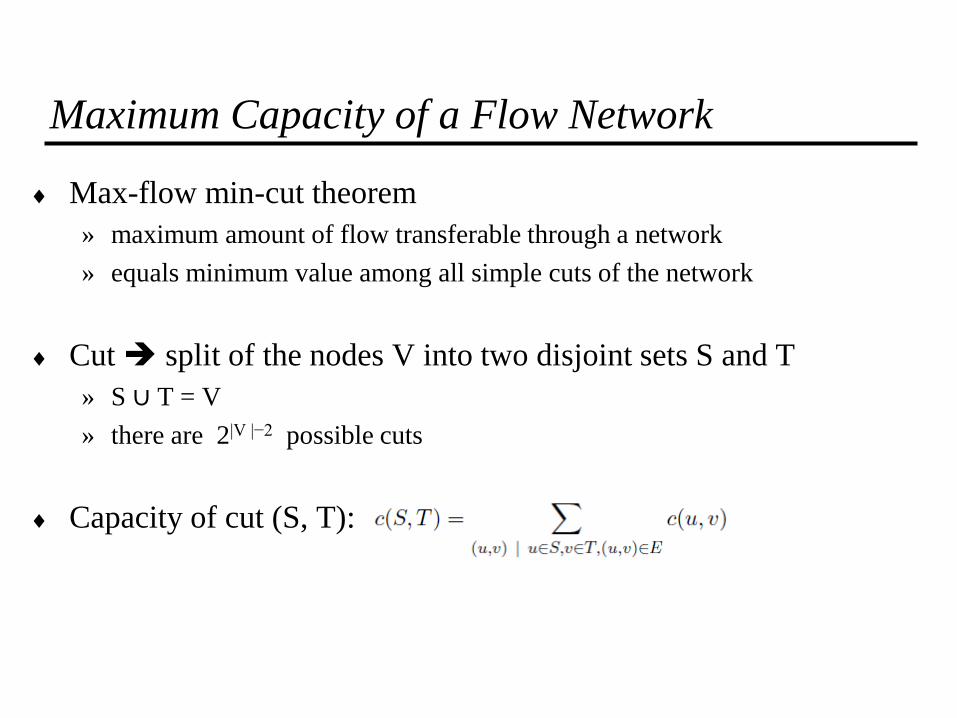
Maximum Capacity of a Flow Network

Max-flow min-cut theorem

» maximum amount of flow transferable through a network

» equals minimum value among all simple cuts of the network

Cut split of the nodes V into two disjoint sets S and T

» S ∪ T = V

» there are 2|V |−2 possible cuts

Capacity of cut (S, T):

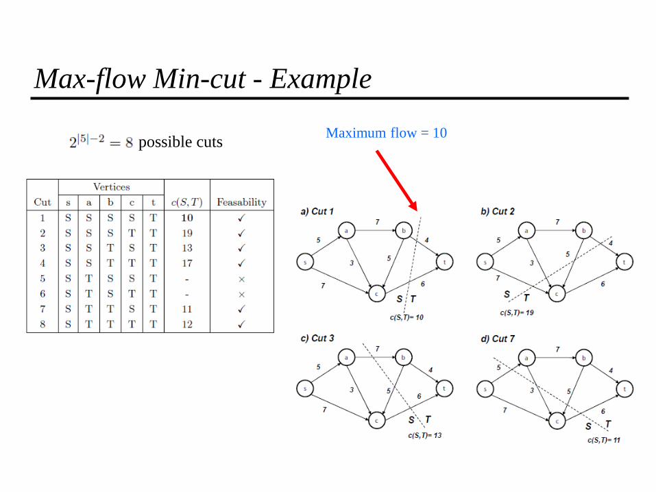
Max-flow Min-cut - Example

Maximum flow = 10 possible cuts

Traffic Management – Packet Level, Flow Level

Time Scales

Packet Level

» Queueing & scheduling at multiplexing points

» Determines performance offered to packets over a short time scale (ms)

Flow Level

» Management of traffic flows & resource allocation ( ms to s)

» Matching traffic flows to available resources

Flow-Aggregate Level

» Routing of aggregate traffic flows across the network (min to days)

» Efficient utilization of resources; meeting of service levels

» Traffic Engineering

1 2 N N – 1

Packet buffer

…

End-to-End QoS

Packet traversing network

» encounters delay and possible loss

» at various multiplexing points

End-to-end performance is the

accumulation of per-hop performances

Quality of Service and Scheduling

End-to-End QoS

» Packet delay, packet loss

» Performance level can be engineered by

– Buffer control, bandwidth control

– Admission control of traffic entering network

Scheduling Concepts: fairness, priority

Fair Queueing

» Weighted Fair Queuing (WFQ)

» Packetized Generalized Processor Sharing (PGPS)

Guaranteed Service: WFQ, Rate-control

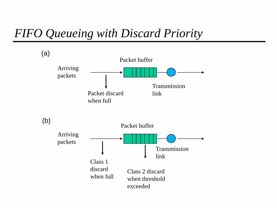
FIFO Queueing

All packet flows share the same buffer

Transmission Discipline: First-In, First-Out

Buffering Discipline » Discard arriving packets if buffer is full

» Random discard

» Discard head-of-line (i.e. oldest, packet)

Packet buffer

Transmission

link

Arriving

packets

Packet discard

when full

FIFO Queueing

Cannot provide differential QoS to different packet flows

Statistical delay guarantees via load control

» Restrict number of flows allowed (connection admission control)

» Difficult to determine performance delivered

Finite buffer determines a maximum possible delay

Buffer size determines loss probability

» Depends on arrival & packet length statistics

Packet buffer

Transmission

link

Arriving

packets

Packet discard

when full

Packet buffer

Transmission

link

Arriving

packets

Class 1

discard

when full Class 2 discard

when threshold

exceeded

(a)

(b)

FIFO Queueing with Discard Priority

Head Of Line (HOL) Priority Queueing

High priority queue serviced until empty

High priority queue has lower waiting time

Buffers can be dimensioned for different loss probabilities

Surge in high priority queue can cause low priority queue to saturate

Transmission

link

Packet discard

when full

High-priority

packets

Low-priority

packets

Packet discard

when full

When

high-priority

queue empty

HOL Priority Features

Provides differential QoS

High-priority classes can

» get all the bandwidth

» starve lower priority classes

De

lay

Per-class loads

Earliest Due Date Scheduling

Queue in order of “due date”

» packets requiring low delay get earlier due date

» packets without delay get indefinite or very long due dates

Sorted packet buffer

Transmission

link

Arriving

packets

Packet discard

when full

Tagging

unit

Fair Queueing /

Generalized Processor Sharing

Each flow has its own logical queue

» prevents hogging; allows differential loss probabilities

C bit/s allocated equally among non-empty queues

» transmission rate = C / n(t), where n(t)= # non-empty queues

Idealized system assumes fluid flow from queues

Implementation requires approximation

» simulate fluid system; sort packets according to completion time in ideal system

C bit/s

Transmission

link

Packet flow 1

Packet flow 2

Packet flow n

Approximated bit-level

round robin service

…

…

Buffer 1

at t=0

Buffer 2

at t=0

1

t 1 2

Fluid-flow system:

both packets served

at rate 1/2

Both packets

complete service

at t = 2

0

1

t 1 2

Packet-by-packet system:

buffer 1 served first at rate 1;

then buffer 2 served at rate 1.

Packet from buffer 2

being served

Packet from

buffer 1 being

served

Packet from

buffer 2 waiting

0

Fluid Flow System

Buffer 1

at t=0

Buffer 2

at t=0

2

1

t

3

Fluid-flow system:

both packets served

at rate 1/2

Packet from buffer 2

served at rate 1

0

2

1

t 1 2

Packet-by-packet fair queueing:

buffer 2 served at rate 1

Packet from

buffer 1 served

at rate 1

Packet from

buffer 2 waiting

0 3

Fluid Flow

Buffer 1

at t=0

Buffer 2

at t=0 1

t

1 2

Fluid-flow system:

packet from buffer 1

served at rate 1/4;

Packet from buffer 1

served at rate 1

Packet from buffer 2

served at rate 3/4 0

1

t

1 2

Packet from buffer 1 served at rate 1

Packet from

buffer 2

served at rate 1

Packet from

buffer 1 waiting

0

Packet-by-packet weighted fair queueing:

buffer 2 served first at rate 1;

then buffer 1 served at rate 1

Fluid Flow with Weights

3/4

1/4

Packetized GPS/WFQ

Compute packet completion time in ideal system

» add tag to packet

» sort packet in queue according to tag

» serve according to HOL

Sorted packet buffer

Transmission

link

Arriving

packets

Packet discard

when full

Tagging

unit

Bit-by-Bit Fair Queueing

Assume n flows, n queues

1 round = 1 cycle serving all n queues

If each queue gets 1 bit per cycle

Round number = number of cycles of service that have been completed

If packet arrives to idle queue:

Finishing time = round number + packet size in bits

If packet arrives to active queue:

Finishing time = finishing time of last packet in queue + packet size

rounds Current Round #

Buffer 1

Buffer 2

Buffer n

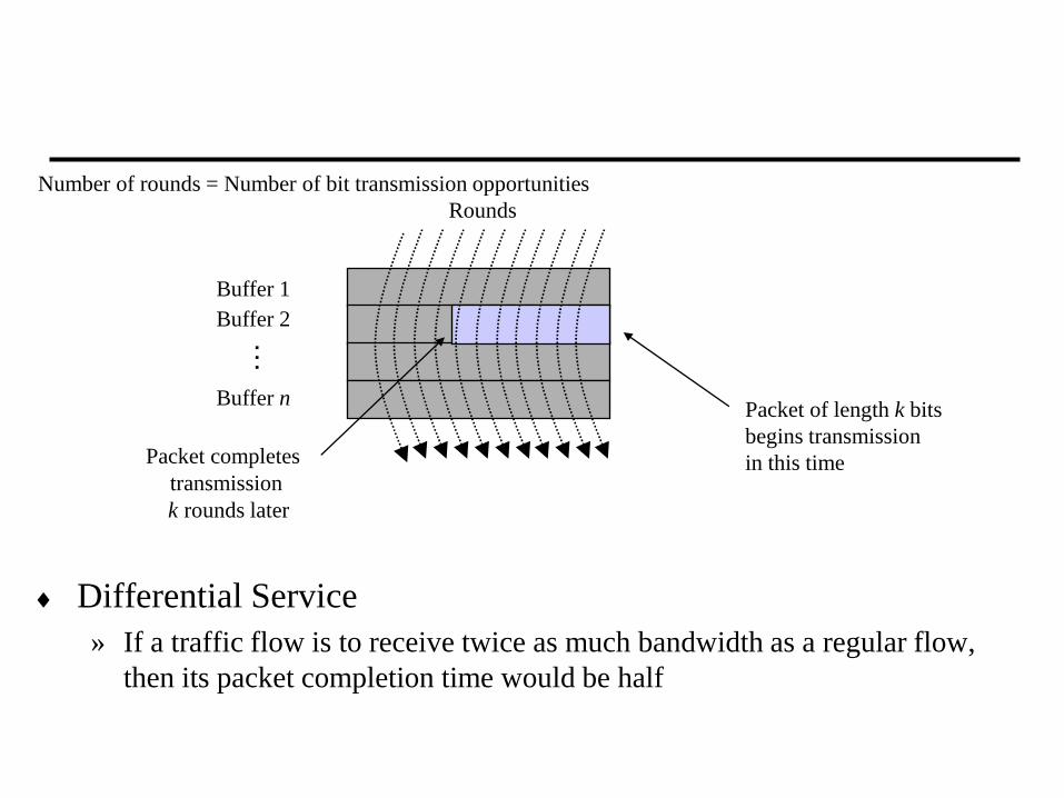
Number of rounds = Number of bit transmission opportunities

Rounds

Packet of length k bits

begins transmission

in this time Packet completes

transmission

k rounds later

…

Differential Service

» If a traffic flow is to receive twice as much bandwidth as a regular flow,

then its packet completion time would be half

F(i,k,t) = finish time of kth packet that arrives at time t to flow i

P(i,k,t) = size of kth packet that arrives at time t to flow i

R(t) = round number at time t

Fair Queueing:(take care of both idle and active cases)

F(i,k,t) = max{F(i,k-1,t), R(t)} + P(i,k,t)

Weighted Fair Queueing:

F(i,k,t) = max{F(i,k-1,t), R(t)} + P(i,k,t)/wi

rounds Generalize so R(t) continuous, not discrete

R(t) grows at rate inversely

proportional to n(t)

Computing the Finishing Time

Traffic Management at the Flow Level

Network Congestion

Congestion Control

» Preventive: Scheduling & Reservations

» Reactive: Detect & Discard

Congestion occurs

when a surge of traffic

overloads network

resources

4

8

6 3

2

1

5 7

Congestion

Offered load

Thro

ughput

Controlled

Uncontrolled

Ideal effect of congestion control:

resources used efficiently up to

capacity available

Ideal Congestion Control

Congestion Control

Open loop

Closed loop

Open-Loop Control

Network performance is guaranteed

to all traffic flows that have been admitted into the network

Initially for connection-oriented networks

Key Mechanisms

» Admission Control

» Policing

» Traffic Shaping

» Traffic Scheduling

Time

Bit

/s

Peak rate

Average rate

Typical bit rate demanded by a

variable bit rate information

source

Admission Control

Flow negotiates contract with network

Specify requirements

» Offered traffic (traffic contract)

– Peak, Average, Min Bit rate

– Maximum burst size

» QoS required – Delay, Loss

Network computes resources needed

» Effective bandwidth

If flow is accepted:

network allocates resources to ensure QoS

as long as source conforms to contract

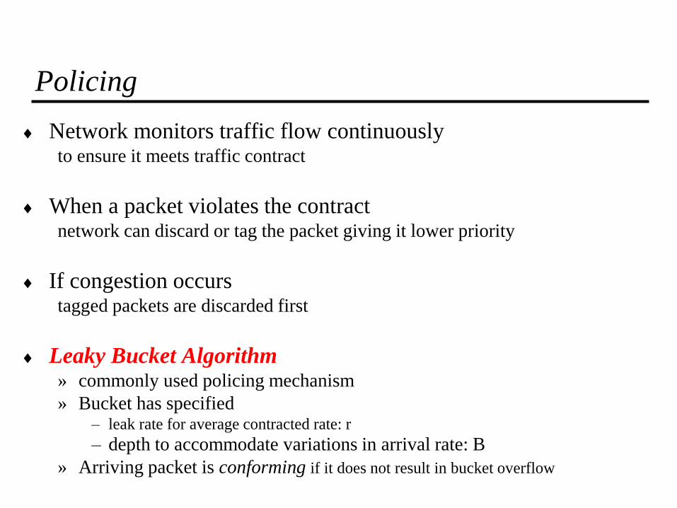
Policing

Network monitors traffic flow continuously to ensure it meets traffic contract

When a packet violates the contract network can discard or tag the packet giving it lower priority

If congestion occurs tagged packets are discarded first

Leaky Bucket Algorithm » commonly used policing mechanism

» Bucket has specified – leak rate for average contracted rate: r

– depth to accommodate variations in arrival rate: B

» Arriving packet is conforming if it does not result in bucket overflow

Leaky Bucket algorithm can be used to police arrival rate of a packet stream

water drains at

a constant rate

leaky bucket

water poured

irregularly Leak rate corresponds to long-

term rate

Bucket depth corresponds to

maximum allowable burst arrival

1 packet per unit time

Assume constant-length packet

Let X = bucket content at last conforming packet arrival

Let ta – last conforming packet arrival time = depletion in bucket

Leaky Bucket Algorithm

I

B

Bucket

content

Time

Time

Packet

arrival

Nonconforming

* * * * * * * * *

I = 4, B=10, L=B-I=6

Non-conforming packets not allowed into bucket, hence not

included in calculations

Leaky Bucket Example

Arrival of a packet at time ta

X’ = X - (ta - LCT)

X’ < 0?

X’ > L?

X = X’ + I

LCT = ta

conforming packet

X’ = 0

Nonconforming

packet

X = value of the leaky bucket counter

X’ = auxiliary variable

LCT = last conformance time

Yes

No

Yes

No

Depletion rate:

1 packet per unit time

L=B-I

I = increment per arrival,

nominal interarrival time

Leaky Bucket Algorithm

Interarrival time Current bucket

content

arriving packet

would cause

overflow

empty

Non-empty

conforming packet

Tagged or

dropped

Untagged traffic

Incoming

traffic

Untagged traffic

PCR = peak cell rate

CDVT = cell delay variation tolerance

SCR = sustainable cell rate

MBS = maximum burst size

Leaky bucket 1

SCR and MBS

Leaky bucket 2

PCR and CDVT

Tagged or

dropped

Dual leaky bucket to police PCR, SCR, and MBS:

Dual Leaky Bucket

Network C Network A Network B

Traffic shaping Traffic shaping Policing Policing

1 2 3 4

Traffic Shaping

Networks police the incoming traffic flow

Traffic shaping is used to ensure that a packet stream

conforms to specific parameters

Networks can shape their traffic prior to passing it to

another network

Incoming traffic Shaped traffic Size N

Packet

Server

Leaky Bucket Traffic Shaper

Buffer incoming packets

Play out periodically to conform to parameters

Surges in arrivals are buffered & smoothed out

Possible packet loss due to buffer overflow

Too restrictive, since » conforming traffic does not need to be completely smooth

Leaky Bucket Traffic Shaper

Controls the maximum instantaneous rate (leak rate) r of a flow

» accepts bursty traffic on its input

» eliminates bursts on the output

While the buffer is not empty

» the output flow is periodic (T = 1 / r),

» with rate r

Maximum accepted Burst Size

» MBS = B * R / (R – r) for R > r

Incoming traffic Shaped traffic Size N

Size b

Tokens arrive

periodically

( r )

Server

Packet

Token

Token Bucket Traffic Shaper

Token rate regulates transfer of packets

If sufficient tokens available, packets enter network without delay

b determines how much burstiness allowed into the network

An incoming packet must

have sufficient tokens

before admission into the

network

The token bucket constrains the traffic from a

source to be limited to b + r t bits in an interval of

length t

b bytes instantly

t

r bytes/second

Token Bucket Shaping Effect

b + r t

Packet transfer with Delay Guarantees

Assume fluid flow for information

Token bucket shaper allows burst of b bytes @1; then r byte/s » Since R>r, buffer content @ 1 never greater than b byte

» Thus, delay @ mux < b/R

Rate into second mux is r<R, so bytes are never delayed

b

R b

R - r

(b) Buffer

occupancy at 1

0

Empty

t t

Buffer

occupancy at 2

A(t) = b+rt

R(t)

No backlog of

packets

(a)

1 2

Token Shaper

Bit rate > R > r

e.g., using WFQ

b

R(t)

Delay Bounds with WFQ / PGPS

Assume

» traffic shaped (token bucket) to parameters b & r

» schedulers give flow at least rate R>r

» H hop path

» m is maximum packet size for the given flow

» M maximum packet size in the network

» Rj transmission rate in jth hop

Maximum end-to-end delay experienced by a packet from flow i is

H

j jR

M

R

mH

R

bD

1

)1(

Scheduling for Guaranteed Service

Suppose guaranteed bounds on end-to-end delay across the

network are to be provided. Then

» Call admission control procedure is required

to allocate resources & set schedulers

» Traffic flows from sources must be shaped/regulated

so that they do not exceed their allocated resources

Strict delay bounds can be met

Classifier

Input

driver Internet

forwarder

Pkt. scheduler

Output driver

Routing

Agent

Reservation

Agent

Mgmt.

Agent

Admission

Control

[Routing database] [Traffic control database]

Current View of Router Functions

Closed-Loop Control

Congestion control

» Feedback information to regulate flow from sources into network

» Based on buffer content, link utilization, …

» Examples: TCP at transport layer; congestion control at ATM level

End-to-end vs. Hop-by-hop

» Delay in effecting control

Implicit vs. Explicit Feedback

» Source deduces congestion from observed behavior

» Routers/switches generate messages alerting to congestion

Source Destination

Feedback information

Packet flow

Source Destination

(a)

(b)

End-to-End vs. Hop-by-Hop Congestion Control

TCP – Congestion Control

End-to-end, Implicit

Main idea » each source determines its capacity

» based on criteria enabling – flow fairness

– efficiency

Received ACKs regulate packet transmission they are the source clock

Additive Increase/Multiplicative Decrease

Changes in channel capacity adjustment of transmission rate

New variable per connection CongestionWindow

Bitrate (byte/s) CongestionWindow/RTT

Objective

» If network congestion decreases CongestionWindow increases

» If network congestion increases CongestionWindow decreases

Additive Increase/Multiplicative Decrease

How does the source know if/when the network is in congestion?

By timeout!

» wired link low BER low FER

» timeout occurrence loss of packet

» packet loss buffer in router is full congestion

Additive Increase/Multiplicative Decrease

Algorithm

» increases CongestionWindow by 1 segment

– for each RTT (Round Trip Time) additive increase

» divide CongestionWindow by 2

– when there is a packet loss multiplicative decrease

Source Destination

…

Additive Increase/Multiplicative Decrease

Saw-tooth behavior

60

20

1.0 2.0 3.0 4.0 5.0 6.0 7.0 8.0 9.0

KB

T ime (seconds)

70

30

40

50

10

10.0

Slow Start

Objective

» determine the available capacity

Behaviour

» start by CongestionWindow = 1 segment

» double CongestionWindow by each RTT

Source Destination

…

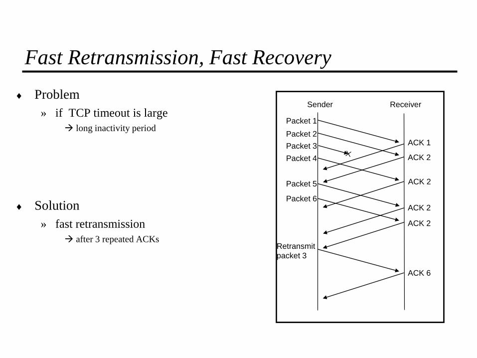
Fast Retransmission, Fast Recovery

Problem

» if TCP timeout is large

long inactivity period

Solution

» fast retransmission

after 3 repeated ACKs

Packet 1

Packet 2

Packet 3

Packet 4

Packet 5

Packet 6

Retransmit

packet 3

ACK 1

ACK 2

ACK 2

ACK 2

ACK 6

ACK 2

Sender Receiver

TCP – Slow Start

Slow Start

» Sender starts with CongestionWindow=1sgm

» Doubles CongestionWindow by RTT

When a segment loss is detected, by timeout

» threshold = ½ congestionWindow(*)

» CongestionWindow=1 sgm

(router gets time to empty queues)

» Lost packet is retransmitted

» Slow start while

congWindow<threshold

» Then Congestion Avoidance phase

Source Destination

…

(*) - in fact FlightSize, the amount of outstanding data

Congestion Avoidance

Congestion Avoidance (additive increase)

» increments congestionWindow by 1 sgm, per RTT

Detection of segment loss, by reception of 3 duplicated ACKs

» Assumes packet is lost,

– Not by severe congestion, because following segments have arrived

» Retransmits lost packet

» CongestionWindow=CongestionWindow/2

» Congestion Avoidance phase

Source Destination

…

60

20

1.0 2.0 3.0 4.0 5.0 6.0 7.0 8.0 9.0

KB

T ime (seconds)

70

30 40 50

10

10.0

Desirable Bandwidth Allocation –

Max-min fairness

Fair use gives bandwidth to all flows (no starvation)

» Max-min fairness gives equal shares of bottleneck

Bottleneck link

max-min fair: maximizes the minimum bandwidth flows get

Desirable Bandwidth Allocation –

Bitrates along the time

CN5E by Tanenbaum & Wetherall, © Pearson Education-Prentice Hall and D. Wetherall, 2011

Bitrates must converge quickly when traffic patterns change

Flow 1 slows quickly

when Flow 2 starts

Flow 1 speeds up

quickly when Flow 2

stops

Homework

Review slides

Read from Leon-Garcia

» Chapter 7 – Packet Switching Networks

Read from Tanenbaum

» TCP – Congestion control

For formal analysis of these topics

» Routing:

– Bertsekas & Gallager, Data Networks

» Traffic and resource management:

– Anurag Kumar, D. Manjunath, Joy Kuri, Communication Networking - An Analytical

Approach, Elsevier, 2004