Commodity Spot Prices: An Exploratory Assessment of Levels and Volatilities 1 Margaret E. Slade Department of Economics The University of Warwick and Henry Thille Department of Economics The University of Guelph November 2002 Abstract: In this paper, we integrate real (product market) and financial (futures market) aspects of commodity trading and assess how the characteristics of each market affect the distribution of commodity prices. In particular, we attempt to explain the level and volatility of the prices of the six commodities that were traded on the London Metal Exchange in the 1990s. The theories that we examine can be grouped into three classes. The first considers how product–market structure and futures– market trading jointly affect spot–price levels, the second assesses whether futures–market trading destabilizes spot–market prices, and the third relates the arrival of new information to both price volaility and the volume of trade. We find support for traditional market–structure models of price levels but not of price stability. In addition, although we find a positive relationship between futures trading and price instability, the link appears to be indirect via a common causal factor. Journal of Economic Literature classification numbers: D43, G13, L13, L71 Keywords: Commodity prices, horizontal concentration, destabilizing speculation, spot markets, futures markets. 1 This research was supported by grants from the Social Sciences and Humanities Research Council of Canada. We would like to thank Joris Pinkse for helpful suggestions, Kazuko Kano for valuable research assistance, and participants in the University of British Columbia’s Finance and Applied Micro workshops and the Gianninni Foundation Lectures at UC Davis and Berkeley for thoughtful comments.

Welcome message from author
This document is posted to help you gain knowledge. Please leave a comment to let me know what you think about it! Share it to your friends and learn new things together.
Transcript
Commodity Spot Prices:An Exploratory Assessment of Levels and Volatilities1
Margaret E. Slade
Department of EconomicsThe University of Warwick
and
Henry Thille
Department of EconomicsThe University of Guelph
November 2002
Abstract:
In this paper, we integrate real (product market) and financial (futures market) aspects of commoditytrading and assess how the characteristics of each market affect the distribution of commodity prices.In particular, we attempt to explain the level and volatility of the prices of the six commoditiesthat were traded on the London Metal Exchange in the 1990s. The theories that we examinecan be grouped into three classes. The first considers how product–market structure and futures–market trading jointly affect spot–price levels, the second assesses whether futures–market tradingdestabilizes spot–market prices, and the third relates the arrival of new information to both pricevolaility and the volume of trade. We find support for traditional market–structure models of pricelevels but not of price stability. In addition, although we find a positive relationship between futurestrading and price instability, the link appears to be indirect via a common causal factor.
Journal of Economic Literature classification numbers: D43, G13, L13, L71
Keywords: Commodity prices, horizontal concentration, destabilizing speculation, spot markets, futures
markets.
1 This research was supported by grants from the Social Sciences and Humanities Research Council of Canada. Wewould like to thank Joris Pinkse for helpful suggestions, Kazuko Kano for valuable research assistance, and participantsin the University of British Columbia’s Finance and Applied Micro workshops and the Gianninni Foundation Lecturesat UC Davis and Berkeley for thoughtful comments.

1 Introduction
The behaviour of commodity prices is a subject that has received considerable attention from aca-demics; it is also a major concern for producers and consumers. Indeed, many producer countriesdepend on revenue from their commodity exports to support their growth and industrialization,whereas consumer countries depend on commodity imports to fuel their production. Moreover, onehas only to look at the history of the formation of stockpiles and other schemes that attempt tostabilize prices, as well as the rise and fall of cartels and producer organizations that attempt to in-crease prices, to realize that the stakes are high.2 It is therefore not surprising that economists havedevised and tested models that explain how commodity–price distributions — means and variances— are determined. Researchers from different subdisciplines, however, model price determinationin very different ways.
Most commodity markets are distinguished by the fact that there is a spot market in whichthe physical product is sold — the real market — as well as a futures market in which contractsfor future delivery of the product are sold — the financial market.3 In this paper, we considerboth real and financial markets, and we look at spot–price formation from several points of view.The theories that we examine can be grouped into three broad classes. The first considers howproduct–market structure and futures–market trading jointly affect spot–price levels, the secondassesses whether futures–market trading destabilizes spot–market prices, and the third relates thearrival of new information to both price volaility and the volume of trade.
We evaluate the models from the three strands of the literature in an integrated framework.However, since there are many theories that attempt to explain commodity–price behavior, theapproach that we take is descriptive rather than structural. In other words, we seek to determinewhich models are consistent with the data and which are not. Furthermore, we ask if there areempirical regularities that cannot be explained by any of the theories.
It is important to disentangle the effects that the two markets have on price levels and volatilities.Indeed, government agencies have some control over the product–market structure and take an activerole in policing concentration in the real market. However, although they regulate the terms of tradein futures markets, governments are usually unwilling to control the volume of trade and tend tointervene in financial markets only in extreme situations.
The markets that we study are for the six metals that were traded on the London Metal Exchange(LME) during the 1990s: aluminum, copper, lead, nickel, tin, and zinc. By considering multiplecommodities, we obtain cross–sectional variation in both product–market structure and financial–market liquidity. By limiting attention to a set of related commodities, however, we are able tohold the financial–market microstructure and the set of contracts under which the commoditieswere traded constant and can thus focus on the variables of interest. With this task in mind, weassembled a panel of data that includes both financial and real variables. This panel allows us toassess the theoretical predictions concerning both time–series and cross–sectional variation in pricedistributions.
Our data come from two sources: financial variables such as turnover and open interest wereobtained from the LME, whereas real data on the activities of firms were provided by the RawMaterials Group. We use the former to characterize the liquidity and depth of the futures market,
2 Perhaps the best example of an organization that attempted to influence the level and stability of the price ofa commodity in recent years is the International Tin Council. See, e.g., Anderson and Gilbert (1988). For a moregeneral account of commodity agreements, see Gordon–Ashworth (1984).
3 We make no distinction between futures and forward markets. The London Metal Exchange has features of both.
1
whereas we use the latter to construct concentration indices and other indicators of the structure ofthe product market.
The first data source is fairly standard. The second, however, is more unusual. Indeed, mostdata–collection agencies publish statistics by geographic region, and those data contain no informa-tion on market structure. The Raw Materials Group, in contrast, keeps track of the activities ofmining companies. In particular, it tracks mergers and other changes in the complex linkages amongmining and refining firms and is consequently a unique source of data on who owns whom.
To anticipate, we find considerable support for traditional market–structure models of pricelevels but not of price stability. In addition, although we find a positive relationship between futurestrading and price instability, there is no evidence of a direct link. Instead, the relationship appearsto be due to a common causal factor such as the arrival of new information.
The organization of the paper is as follows. In the next section, we discuss the theories that formthe basis of our empirical tests and we briefly describe previous tests of those theories. Section 3describes the London Metal Exchange, section 4 discusses the data, section 5 develops the empiricalmodel, and section 6 presents the empirical results. Finally, section 7 concludes.
2 The Models
In this section, we discuss industrial–organization (IO) models of commodity prices, whose principalpredictions are concerned with price levels, and economic and financial models of the volume offutures–market trading, whose principal predictions are concerned with price stability.
2.1 Product–Market Structure
2.1.1 The Price Level
Many IO models predict that, at least when products are homogeneous as is the case with com-modities, the price level (relative to marginal cost) is determined to a large extent by the structureof the industry. Moreover, industry structure is often summarized by some notion of the numberand size distribution of the firms in the market. Nevertheless, the sensitivity of prices to industrystructure depends very much on the game that the firms are assumed to play.
To illustrate, consider the simple Cournot and Bertrand models of spot–market trading. In theCournot model, firms play a quantity game and price rises with industry concentration, whereasin the Bertrand model, firms play a price game and marginal–cost pricing prevails as long as themarket is not monopolized.
More recently, economists have incorporated futures–market trading into spot–market games.4
For example, Allaz (1992) shows that, in a two-period Cournot game with futures trading in the firstperiod and spot trading in the second, the introduction of a futures market causes the spot price tofall from the Cournot level to one that is closer to Betrand. The reason is simple: futures tradingreduces the number of units that are sold in the spot market, which increases the marginal revenuefrom each unit sold and causes firms to increase output. Nevertheless, although the dependence ofthe price level on industry concentration is weakened in this model, the link is still positive.
Allaz and Villa (1993) modify the two–period model to encompass multiple periods of futurestrading followed by a single period of spot trading. They show that as the number of periods
4 For a survey of the earlier literature on this subject, see Anderson (1991).
2

of futures trading increases, or equivalently as the period between trades falls, price approachesmarginal cost. Given that trading in most futures markets is continuous, their model, like theBertrand model, predicts that marginal–cost pricing will prevail, regardless of market structure. Inother words, the price–level/market–structure link is broken.5
2.1.2 The Volatility of Prices
There are many informal models that suggest that prices should be more stable in imperfectlycompetitive markets. For example, firms might refrain from changing prices in response to cost anddemand shocks for fear of triggering price wars, or kinked–demand curves might lead to ranges ofmarginal–cost changes that are not met with price changes. In addition to these informal stories,Newbery develops two formal links between market structure and price stability.
In the first model, Newbery (1984) contrasts the degree of price stabilization (via storage) thatfirms undertake in perfectly competitive markets with that undertaken by a dominant firm. Whenchoosing the amount to store, firms set the marginal cost of storage equal to the marginal benefit.The implications for price stability arise because perfectly competitive firms’ marginal benefits arebased on price, whereas a dominant firm’s benefit is based on marginal revenue. Newbery showsthat, when demand is linear, storage and thus price stability increases with a dominant firm’s marketshare.6
In the second model, Newbery (1990) introduces the possibility of futures trading. He notes that,since futures markets reduce risk, they encourage fringe firms to supply more output and thus reducethe spot price. A dominant firm or cartel might therefore want to undertake excessive storage orprice stabilization in order to undermine the futures market. With both models, therefore, marketconcentration and price instability are negatively related.
2.1.3 The Predictions and Tests of Those Predictions
The testable predictions of the market–structure models of commodity–price determination aresummarized in Table 1. To reiterate, those models predict that prices should not be lower or lessstable in more concentrated industries.
On the empirical side, there is a very large literature on the relationship between product–marketconcentration and firm profitability (see Schmalensee 1989 for a survey). Those studies, which tendto find a positive but weak relationship between the two, do not assess how futures–market tradingaffects that relationship. In addition, if profits are higher in concentrated markets, it could be dueto market power that allows firms to raise prices or to economies of scale that allow them to lowercosts, and it is difficult to disentangle the two effects. Since we assess how market structure is relatedto price levels, we do not confound the effects.
A few empirical researchers have also assessed the relationship between market structure andprice stability.7 Those studies tend to find that price variability is lower in concentrated industries.
5 Thille and Slade (2000) question why the spot market meets just once in the Allaz and Villa model. In particularthey show that, if the inability of firms to change output is due to adjustment costs, output is lower and prices arehigher than in the two–stage game, contrary to the Allaz and Villa finding.
6 More generally, if storage and arbitrage can also be undertaken by competitive intermediaries, the presence ofimperfect competition tends to reduce price instability regardless of the shape of the demand curve.
7 See, e.g., Carlton (1986), Slade (1991), and Domberger and Fiebig (1993).
3

2.2 Futures–Market Trading
2.2.1 The Price Level
There are a number of ways in which the intensity of activity in the financial market can affect thespot–price level. For example, futures markets allow risk–averse participants, both producers andconsumers, to hedge exposure to risk. When hedging is undertaken by producers, the supply of thespot commodity is affected, whereas when it is undertaken by consumers, demand is affected.8 Sincehedging changes both demand and supply, the direction of the net effect is ambiguous. Nevertheless,since producer hedging is apt to be more important than consumer hedging, one might expectincreased trading to lower prices.
In addition, in the absence of futures markets, commodity trading can be very fragmented.Futures markets, however, concentrate trading in one location. They therefore reduce informationand other transactions costs, which can also lead to lower prices.
2.2.2 The Volatility of Prices
(De)stabilizing SpeculationThe introduction of a futures market serves two important functions, it reduces risk and it
increases the amount of information that flows into the market. It is therefore not surprising thateconomists have focused on those two functions in attempting to discover whether futures–markettrading destabilizes spot prices.
Researchers often seek to determine how the introduction of a futures market, which facilitatesthe entry of speculators, affects the spot price of a commodity. In other words, they examine anall–or–nothing situation in which there is either a futures market or there is not. However, as Stein(1987) points out, it is also interesting to ask whether more speculation is better than less. In ourempirical work, we address the second question. However, most of the arguments that are advancedin the all–or–nothing literature extend easily to the more–or–less issue.
Many market participants believe that futures trading is destabilizing. Nevertheless, most ofthe early economic models that examined the issue concluded that the opposite was true. Forexample, Turnovsky (1979) and Turnovsky and Campbell (1985) focus on the risk–reduction effectand note that, since futures markets reduce the price risk of holding inventories, larger inventoriesare held and prices tend to stabilize as a consequence. In their model inventory holding is notstochastic. Kawai (1983), however, shows that when storage is subject to shocks, increased storagecan destabilize prices. Finally, Newbery (1987) builds a model in which risk–reduction encouragesproducers to undertake more risky investment projects, and risky investment destabilizes spot prices.Furthermore, he points out that, in general, futures markets encourage risk taking and that the effecton the spot price depends on whether the risky activity tends to be stabilizing or destabilizing.
Early models of the information effect also led to the conclusion that the introduction of afutures markets stabilizes spot prices. For example, both Cox (1976) and Danthine (1978) notethat speculators arrive with new information and show that better information lowers spot–pricevolatility. However, Stein (1987) points out that a change in the information content of prices inflictsan externality on traders, and that this externality can be either positive or negative. In other words,even when all traders are rational, there can be a misinformation effect that can destabilize prices.
8 Newbery and Stiglitz (1981) show that, for example, in an uncertain environment risk-averse producers increasesupply when a futures market is added, and price falls as a consequence.
4
Financial Volume–Volatility ModelsMost financial models of price volatility attempt to explain the behavior of futures prices. Nev-
ertheless, since spot and futures prices are closely related,9 those models offer insights into thebehavior of the former as well as the latter.
Most theories of price volatility that have been proposed by financial economists are informa-tional models. Those models assess the impact of information arrival on financial markets, whereinformation acquisition can be exogenous or endogenous. Early models focused on the joint distri-bution of price changes and trading volume, where both are determined by the exogenous arrival ofinformation. For example, the ‘Mixture–of–Distributions Hypothesis’ (Clark 1973, Epps and Epps1976) postulates that price changes are sampled from a mixture of normal distributions with thevolume of transactions or the number of information arrivals acting as the mixing variable. In thosemodels, the variance of returns in a period is positively related to the volume of trade in that period,not through any causal link, but because both are determined by an underlying latent variable orcommon causal factor.
More recent models of the volume–volatility relationship, in which information is asymmetric,include both informed (insider) and uninformed (liquidity or noise) traders (e.g., Kyle 1985 and1989, Admati and Pfleiderer 1988, Wang 1994). Admati and Pfleiderer note that if informed anduninformed traders have timing discretion, they will prefer to trade when the volume of transactionsis larger, since the impact of their activity on prices will be smaller. In their model, as with theearlier models, information arrival generates trade and volatility. However, there also exists feedbackbetween volume and volatility, since increased volatility induces more trading and increased liquidity,which in turn affect information acquisition.
Most informational models predict that volume and volatility will be positively related. Onecan, however, also obtain a negative relationship. In particular, Pagano (1989) shows how theinteraction between thinness and volatility can lead to multiple equilibria, some with low trade andhigh volatility and some with the reverse. Indeed, markets are often thin because traders are few,which causes prices to be more sensitive to individual trades. Investors are hesitant to trade in suchmarkets, which exacerbates their thinness. Note that thinness is defined here as few traders, notlow volume per se. However, it is often difficult to distinguish between the two empirically.
2.2.3 The Predictions and Tests of Those Predictions
The testable predictions of the theoretical models of futures trading are summarized in Table 2. Toreiterate, most informal stories lead one to expect lower prices in markets in which trading is intense.As to price stability, the predictions from the destabilizing–speculation literature are very mixed.Most volume–volatility models, in contrast, predict that prices will be more volatile in markets withintense trading.
On the empirical side, the relationship between price levels and futures trading has received littleattention, perhaps because there are no sharp theoretical predictions. Nevertheless, Williams (2001)documents a negative relationship between open interest (one of our measures of trading activity)and price for several commodities.
Several empirical researchers have assessed the destabilizing–speculation issue. In particular,they have examined how the introduction of a futures market affects the spot price, and, like the
9 The prices are related by the fact that, at the time when the futures contract matures, arbitrage assures thatthe contract price equals the spot price.
5
theoretical predictions, the empirical results are mixed. For example, Cox (1976) finds that in manymarkets futures trading is stabilizing, whereas Figlewski (1981) and Simpson and Ireland (1985)conclude that the opposite is true.
A much larger number of empirical researchers have assessed the volume–volatility issue. Al-though there is some variation, like the theoretical models, most empirical studies find a positiverelationship between the two variables (see the survey by Karpoff 1987 and, for more recent work,see Tauchen, Zhang, and Liu 1996 and the references therein).10
3 The London Metal Exchange
The commodities that we examine are the six metals that were traded on the London Metal Exchange(LME) during the 1990s: aluminum, copper, lead, nickel, tin, and zinc.11 The LME is by far themost important market for nonferrous metals, with an annual turnover value of about US $2,000billion.
The LME was formally established in 1877 in the wake of the industrial revolution. It flourishedbecause it established a single marketplace with recognized times of trading and standard contracts.The number and identity of the metals that were sold has varied over time. Copper and tin havetraded since the beginning,12 lead and zinc were introduced in 1920, aluminum was introduced in1978, and nickel started trading in 1979. Finally, a silver contract was launched in 1999.13
The LME underwent a major restructuring in 1987. Prior to that date, it was a principals’ market(a market where members acted as principals for the transactions that they concluded across thering and with their clients), whereas afterwards, it became a clearing–house system. The LMEclearing house is an independent body that guarantees transactions between brokers. In particular,the house assumes one side of all trades.
An unusual feature of LME contracts is that they are for delivery on a specific day, which meansthat every day is a delivery date for some contract. Furthermore, contracts are settled on the daythat they are due. This practice can be contrasted with the continuous–settlement practice that isused by many other exchanges.
In addition to to providing hedging opportunities to producers and consumers, the primaryfunctions of the LME are to establish worldwide reference prices and to enable market participantsto take physical delivery. At the LME, each of the six commodities trades in turn for short (five–minute) periods of open outcry among ring–dealing members. Open outcry or ring trading takesplace four times each day on the market floor. In addition, the LME operates a 24–hour marketthrough inter–office trade. After the second floor–trading period, the LME announces a set of officialprices that are used by industry members to write contracts that govern the movement of physicalmetal. Official prices are determined for both cash settlement and futures trading.
In spite of the fact that only a small fraction of LME contracts result in physical delivery, allcontracts assume delivery. For this reason, the LME has established approved warehouses aroundthe world where large stocks of metal are held. The levels of stocks in those warehouses can be used
10 Most empirical studies assess time–series variation in the volume–volatility relationship. However, the predictionsshould also hold in a cross section of markets. To illustrate, with multiple equilibria one might observe some low–trade,high–volatility markets and other markets with the opposite characteristics.
11 For more information on the LME, see their web page at www.lme.co.uk.12 Tin trading was temporarily suspended after the collapse of the International Tin Council but resumed trading
in 1989.13 This was not the first LME silver contract, however.
6
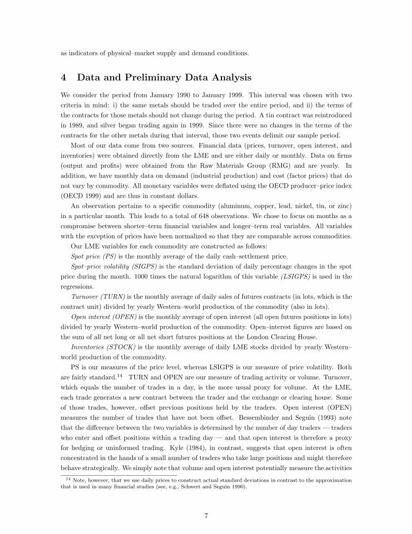
as indicators of physical–market supply and demand conditions.
4 Data and Preliminary Data Analysis
We consider the period from January 1990 to January 1999. This interval was chosen with twocriteria in mind: i) the same metals should be traded over the entire period, and ii) the terms ofthe contracts for those metals should not change during the period. A tin contract was reintroducedin 1989, and silver began trading again in 1999. Since there were no changes in the terms of thecontracts for the other metals during that interval, those two events delimit our sample period.
Most of our data come from two sources. Financial data (prices, turnover, open interest, andinventories) were obtained directly from the LME and are either daily or monthly. Data on firms(output and profits) were obtained from the Raw Materials Group (RMG) and are yearly. Inaddition, we have monthly data on demand (industrial production) and cost (factor prices) that donot vary by commodity. All monetary variables were deflated using the OECD producer–price index(OECD 1999) and are thus in constant dollars.
An observation pertains to a specific commodity (aluminum, copper, lead, nickel, tin, or zinc)in a particular month. This leads to a total of 648 observations. We chose to focus on months as acompromise between shorter–term financial variables and longer–term real variables. All variableswith the exception of prices have been normalized so that they are comparable across commodities.
Our LME variables for each commodity are constructed as follows:Spot price (PS) is the monthly average of the daily cash–settlement price.Spot–price volatility (SIGPS) is the standard deviation of daily percentage changes in the spot
price during the month. 1000 times the natural logarithm of this variable (LSIGPS) is used in theregressions.
Turnover (TURN) is the monthly average of daily sales of futures contracts (in lots, which is thecontract unit) divided by yearly Western–world production of the commodity (also in lots).
Open interest (OPEN) is the monthly average of open interest (all open futures positions in lots)divided by yearly Western–world production of the commodity. Open–interest figures are based onthe sum of all net long or all net short futures positions at the London Clearing House.
Inventories (STOCK) is the monthly average of daily LME stocks divided by yearly Western–world production of the commodity.
PS is our measures of the price level, whereas LSIGPS is our measure of price volatility. Bothare fairly standard.14 TURN and OPEN are our measure of trading activity or volume. Turnover,which equals the number of trades in a day, is the more usual proxy for volume. At the LME,each trade generates a new contract between the trader and the exchange or clearing house. Someof those trades, however, offset previous positions held by the traders. Open interest (OPEN)measures the number of trades that have not been offset. Bessembinder and Seguin (1993) notethat the difference between the two variables is determined by the number of day traders — traderswho enter and offset positions within a trading day — and that open interest is therefore a proxyfor hedging or uninformed trading. Kyle (1984), in contrast, suggests that open interest is oftenconcentrated in the hands of a small number of traders who take large positions and might thereforebehave strategically. We simply note that volume and open interest potentially measure the activities
14 Note, however, that we use daily prices to construct actual standard deviations in contrast to the approximationthat is used in many financial studies (see, e.g., Schwert and Seguin 1990).
7

of different sets of traders and include both measures in our analysis. Finally, STOCK measuressupply/demand imbalance.
Table 3 gives summary statistics for the LME variables. The table shows that daily inventoriesand turnover are very large — on average nearly one tenth of annual world production. The secondhalf of Table 3 presents some statistics of the futures–market data that have been disaggregated bycommodity. Of note is the fact that turnover and open interest are not extremely highly correlated.Furthermore, it is interesting that the two volume measures exhibit different cross–sectional patterns.For example, the commodity with the largest turnover (copper) has only the third largest openinterest. Finally, although there is considerable cross-sectional variation in volatility, there are nomarked cross–sectional patterns in that variable.
The data on firms are more unusual. RMG publishes annual data on the production of eachcommodity by each firm as well as other firm variables such as accounting profits.15 We use thedata for refinery production to construct annual indices of commodity–market concentration as wellas total production. Our annual product–market variables for each commodity are:
Hirschman/Herfindahl index (HHI) is the sum of the squared market shares of individual firms,multiplied by 10,000.
Four–firm concentration ratio (CR4) is the percentage of industry output that is supplied by thefour largest firms in the market.
Western–world production (WWQ) is total annual output of the commodity. This variable isused as a normalization factor (see above).
Summary statistics for the RMG variables also appear in Table 3. The second half of this tableshows that the tin and nickel markets are more concentrated (1000<HHI<1400), whereas the otherfour markets are more competitive (100<HHI<500). Furthermore, turnover is somewhat higher incopper, a relatively competitive industry, whereas open interest is much higher in tin and nickel, therelatively concentrated industries.
We also collected monthly data on demand and supply variables that are common to all com-modities. Except where noted, those variables were found in the OECD Statistics Compendium(1999).
Industrial production (IP) is aggregate industrial output of the OECD countries, 1990 = 100.Energy price (ENP) is an index of energy prices for OECD countries, 1990 = 100.Hourly earnings (WAGE) is an index of hourly earnings for OECD countries, 1990 = 100.Price of mining machinery and equipment (MME) is the US producer–price index for mining
machinery and equipment, 1990 = 100, from CITYBASE.Interest rate (INT) is the average of the following short–term interest rates: US 3–month cer-
tificates of deposit, Japanese 3–month certificates of deposit, French 3–month interbank–loan rate(FIBOR), German 3–month interbank–loan rate, and UK 3–month interbank–loan rate (LIBOR).A real interest rate (RINT) was created by subtracting the rate of inflation in OECD countries fromthe nominal average.
None of the factor–price variables is ideal. Unfortunately, it was not possible to find moredisaggregated monthly data for such a broad geographic region. Summary statistics for the demandand supply variables are also shown in Table 3.
In order to examine time–series patterns in the data, we averaged across commodities using twoweighting schemes — equal and value (revenue) weights. Figures 1 and 2 illustrate the time–series
15 For more information on the Raw Materials Group, see their web page at www.rmg.se.
8

behavior of real spot–price levels and volatilities. There is clearly a downward trend in the price–level series, whereas the volatility graphs are relatively flat. As with volatility, graphs of industryconcentration showed no obvious trend. Both turnover and open interest, however, increased sharplyduring the first half of the decade and flattened out in the second half.
Finally, histograms showed that the price–level distribution is unimodal and symmetric, whereasthe volatility series are skewed to the left. Taking logarithms of volatility, however, removes theskewness.
5 The Empirical Model
5.1 Specification
The general form of the equations that are estimated is
yit = αi + βTmit + γTAit + δTxit + uit, i = 1, . . . , 6, t = 1, . . . , 108, (1)
where i is a commodity, t is a month, yit is a price level or volatility variable (PS or LSIGPS),mit is a vector or scalar of market–structure measures (HHI or CR4), Ait is a vector or scalar offinancial–market–activity variables (TURN or OPEN), xit is a vector of supply/demand variablesthat can include a trend, and uit is a zero–mean random variable. Finally, α = (α1, . . . , α6)T is avector of commodity fixed effects.
There are at least five econometric issues that must be dealt with: the possibility that somevariables might be nonstationary, the issue of endogeneity of some of the explanatory variables, thequestion of whether the specification should be dynamic, the fact that some variables are measuredat monthly intervals whereas others are measured yearly, and the choice of an error–covariancestructure.
First consider the stationarity issue. Of the variables in equation (1), prices are most apt to benonstationary. However, there is little agreement on this issue. In particular, IO researchers oftenassume that prices are stationary, whereas researchers from finance typically assume that they arenot. Furthermore, tests for the presence of unit roots in commodity prices yield conflicting results.16
We do not attempt further tests here. Instead, despite the mixed evidence, we assume that all ofour variables are mean reverting. We do this for two reasons: we feel that the evidence in favorof nonstationarity is not compelling, and we worry that, if we filter our data, our results might besensitive to the filter chosen.
Second, all of the financial variables in our model are apt to be jointly determined and thereforeendogenous. In particular, we believe that trading activity and inventories are jointly determinedwith price levels and volatilities. Furthermore, the endogeneity problem worsens as the periodbetween observations, ∆t, lengthens. We therefore use an instrumental–variables (IV) technique tocorrect for simultaneity.
Although the use of monthly (as opposed to daily or hourly) data exacerbates some problems,it mitigates others. Indeed, many financial models of the volume–volatility relationship focus ondynamic issues. Dynamics can appear in equation (1) in two ways: lagged dependent and explanatoryvariables can be included on the right–hand–side of the equation, and the error, u, can have adynamic specification (e.g., serial correlation and/or heteroskedasticity across time).17 The data
16 Some studies conclude that prices are nonstationary, but others find evidence of mean reversion, e.g., Bessem-binder et. al. (1995), Schwartz (1997), Pindyck (1999), and Slade (2001).
17 In our estimation, we correct for serial correlation of an unknown form.
9

that are used to estimate those financial models, however, are typically daily, and the specificationtypically includes lags of less than two weeks. Furthermore, some researchers find that the temporalrelationship between price variability and trading volume in commodity–futures markets is largelycontemporaneous (e.g., Foster 1995). Given that our data are monthly, dynamics are apt to play aless important role. Furthermore, we face a practical problem in modeling dynamics – most of ourdata are measured at monthly frequencies, but some are measured yearly. Monthly lags of the lattervariables of up to eleven periods could therefore be constant. For these reasons, we specify a staticmodel. Unfortunately, failure to include lagged explanatory variables when appropriate could resultin biased estimates. The use of instruments, however, also overcomes this problem.
To illustrate, consider the possibility that lagged trading activity, Ait−j , j > 0, belongs in (1).If it is inappropriately excluded, it will be incorporated into u. Furthermore, if trading activity isitself autocorrelated, the current value, Ait, will be correlated with u. However, projections of Aitonto the instruments will be not be correlated with u.
Next, consider the frequency of the data. Unlike trading activity, market structure changes veryslowly and can be considered a state variable. Even if we had monthly data on market structure,there would therefore be little month–to–month variation in that data. We model the situation asfollows.
Suppose that there is a single market–structure index18 and that the yearly value of thatindex, M , has two components, one that is specific to commodity i and one that is common toall commodities, MiT = MiT + µT , where T is a particular year. The monthly value is thenmit = MiT +vit, where t is a month in year T , and v is measurement error. Under this specification,equation (1) becomes
yit = αi + βMiT + γTAit + δTxit + ηT + wit, (2)
where ηT is a vector of yearly fixed effects, and wit = uit + βvit. We assume that monthly mea-surement error is mean independent of the yearly market–structure index, E[vit|M ] = 0. However,since contemporaneous correlation between monthly observed activity and unobserved measurementerror, Ait and vit, is likely, the application of OLS to (2) could yield biased estimates. As withdynamic considerations, however, the use of instruments overcomes this problem.
Finally, we must choose a stochastic specification for w. Linkages among commodity marketsimply that shocks to one market can be transmitted to related markets. We therefore expect con-temporaneous correlation in w across commodities, and we specify a full cross–sectional covariancematrix Σ = [σij ], i, j = 1, . . . , 6. The covariance matrix for w is then
Ω = V AR(w) = (Σ⊗ I108), (3)
where ⊗ is the Kronecker product.There are two estimating equations, and one might also want to incorporate correlation in the
shocks across equations (i.e., to estimate a system of seemingly unrelated regressions). However,since the same explanatory variables appear in each equation, estimating a system is no differentfrom estimating each equation separately.
5.2 Estimation
Equation (2) can be written in matrix notation as
y = Zθ + w, (4)18 The same argument holds with a vector of market–structure indices.
10
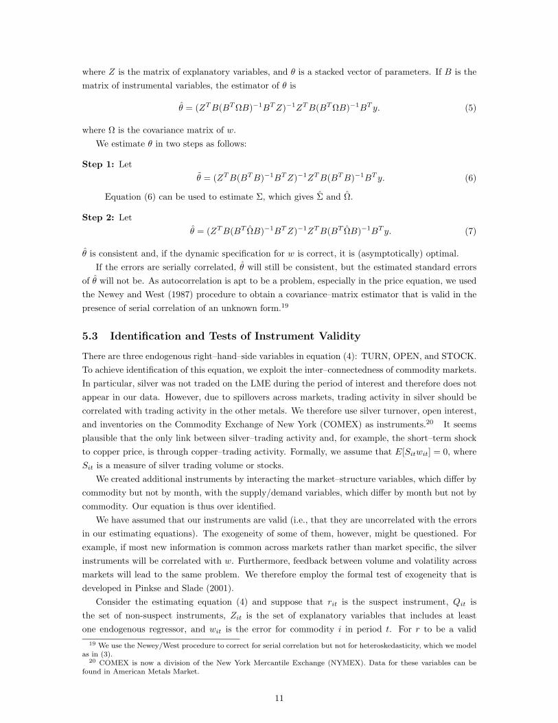
where Z is the matrix of explanatory variables, and θ is a stacked vector of parameters. If B is thematrix of instrumental variables, the estimator of θ is
θ = (ZTB(BTΩB)−1BTZ)−1ZTB(BTΩB)−1BT y. (5)
where Ω is the covariance matrix of w.We estimate θ in two steps as follows:
Step 1: Letθ = (ZTB(BTB)−1BTZ)−1ZTB(BTB)−1BT y. (6)
Equation (6) can be used to estimate Σ, which gives Σ and Ω.
Step 2: Letθ = (ZTB(BT ΩB)−1BTZ)−1ZTB(BT ΩB)−1BT y. (7)
θ is consistent and, if the dynamic specification for w is correct, it is (asymptotically) optimal.If the errors are serially correlated, θ will still be consistent, but the estimated standard errors
of θ will not be. As autocorrelation is apt to be a problem, especially in the price equation, we usedthe Newey and West (1987) procedure to obtain a covariance–matrix estimator that is valid in thepresence of serial correlation of an unknown form.19
5.3 Identification and Tests of Instrument Validity
There are three endogenous right–hand–side variables in equation (4): TURN, OPEN, and STOCK.To achieve identification of this equation, we exploit the inter–connectedness of commodity markets.In particular, silver was not traded on the LME during the period of interest and therefore does notappear in our data. However, due to spillovers across markets, trading activity in silver should becorrelated with trading activity in the other metals. We therefore use silver turnover, open interest,and inventories on the Commodity Exchange of New York (COMEX) as instruments.20 It seemsplausible that the only link between silver–trading activity and, for example, the short–term shockto copper price, is through copper–trading activity. Formally, we assume that E[Sitwit] = 0, whereSit is a measure of silver trading volume or stocks.
We created additional instruments by interacting the market–structure variables, which differ bycommodity but not by month, with the supply/demand variables, which differ by month but not bycommodity. Our equation is thus over identified.
We have assumed that our instruments are valid (i.e., that they are uncorrelated with the errorsin our estimating equations). The exogeneity of some of them, however, might be questioned. Forexample, if most new information is common across markets rather than market specific, the silverinstruments will be correlated with w. Furthermore, feedback between volume and volatility acrossmarkets will lead to the same problem. We therefore employ the formal test of exogeneity that isdeveloped in Pinkse and Slade (2001).
Consider the estimating equation (4) and suppose that rit is the suspect instrument, Qit isthe set of non-suspect instruments, Zit is the set of explanatory variables that includes at leastone endogenous regressor, and wit is the error for commodity i in period t. For r to be a valid
19 We use the Newey/West procedure to correct for serial correlation but not for heteroskedasticity, which we modelas in (3).
20 COMEX is now a division of the New York Mercantile Exchange (NYMEX). Data for these variables can befound in American Metals Market.
11

instrument, w and r must be element–wise uncorrelated, i.e. E[ritwit] = 0. Let PQ = Q(QTQ)−1QT ,M = I−Z(ZTPQZ)−1ZTPQ, V = rTM ΩMT r, where Ω is our estimate of Ω, and w be the residualsfrom an IV estimation using Q (but not r) as instruments. Then, under mild regularity conditionson Ω,
V −1/2rT w = V −1/2rTMw (8)
has a limiting N(0, 1) distribution.If one wants to test more than one instrument at a time, it is possible to use a matrix R instead
of the vector r. Indeed, if V = RTM ΩMTR, the quantity
wTR V −1RT w (9)
has a limiting χ2 distribution with degrees of freedom equal to the number of instruments tested.
5.4 Testing the Theoretical Models
The principal testable predictions of the theoretical models are summarized in Tables 1 and 2.However, unlike the market–structure and destabilizing–speculation models, most of the volume–volatility models were designed to explain trading over very short intervals (hours or days). Con-sequently, one might question whether it is possible to test those models with monthly data. Webelieve that it is possible to rephrase the arguments so that they apply to longer time periods.
To illustrate, consider the Mixture–of–Distributions Hypothesis. Figure 2 shows that somemonths are characterized by high volatility and others by low. Furthermore, if information ar-rival is serially correlated as many believe, there will also be months in which much informationarrives and others in which little arrives. If new information leads to both increased trading activityand larger price changes, volume and volatility will be positively correlated in the monthly data.
It is a little harder to argue that traders with private information or who must hedge for exogenousreasons have timing discretion that extends over months. However, mining and refining companieshedge only a fraction of their output, and the degree to which they hedge is at least partiallyendogenous. They can therefore choose to hedge more intensely when trading is unusually active. Inaddition, most nonferrous mining and refining companies produce more than one metal and can alsochoose which metals to hedge more intensely. They might thus choose to enter those commoditymarkets in which trading activity is heavier. As with intra–day trading, feedback between volumeand volatility can therefore exist in the monthly data. When this is the case, both timing–discretionand endogenous–thinness arguments can be extended to longer periods of time.
Unfortunately, there are more models than testable predictions, which makes it difficult to distin-guish among theories. However, we can exploit our instrumental–variables estimator to distinguishbetween two classes of models that yield the same predictions concerning the relationship betweentrading activity and price volatility. Indeed, with some models (e.g., the destabilizing–speculationand endogenous–timing models) there is a direct link between trading activity and volatility. Fur-thermore, with those models, there can be feedback between the two variables. With other modelssuch as the Mixture–of Distributions, in contrast, there is no direct link between trading and volatil-ity. When the correlation between volume and volatility is driven by an underlying latent variableand there is no direct link, OLS estimates of equation (2) will indicate that volume and volatility arepositively correlated. This correlation will disappear, however, when instruments are used.21 When
21 Our argument assumes that the instruments do not include the latent informational variables, which is apt tobe the case in our application.
12

there is a direct link or feedback, in contrast, the correlation should survive the use of instruments.Figure 3 illustrates our point in the context of an informational model. In this figure, y1 is
volatility, y2 trading activity, and zi is an instrument that shifts yi but not yj , j 6= i. Finally, x isan informational variable that shifts both yi and yj . In the first half of the figure, (A), there is nodirect connection between the two endogenous variables, whereas in the second half, (B), there isfeedback between the two. The figure shows that shifts in one of the instruments (the z’s) will causeboth endogenous variables to move in panel B but not in panel A.
6 Empirical Results
The two equations in the system explain the level and volatility of spot prices. We present two sets ofestimates of each system. The first set consists of OLS regressions, whereas the second is estimatedby the IV method that is described in subsection 5.2. All specifications include cost variables. Tosave on space, however, the coefficients of those variables are not shown.
The price–level equations and some specifications of the volatility equations include commodityfixed effects, which implies that identification is achieved through variation in the time dimension.We also estimate specifications that do not include commodity fixed effects. Those equations areprincipally identified through variation in the cross section. This is true because, with most variables,cross–sectional variation dominates time–series variation.
6.1 The OLS Estimates
The OLS estimates appear in the top halves of Tables 4 and 5. First consider the equations thatexplain spot–price levels (Table 4). Since prices are not comparable across commodities, all spec-ifications for levels include commodity fixed effects that allow means of all variables to differ bycommodity. The four specifications of the equation differ according to the measure of volume ortrading activity that is used and according to the inclusion of yearly fixed effects.22
Table 4 provides strong evidence that a more concentrated industry is associated with higherprices, as the conventional wisdom predicts. Furthermore, prices appear to be higher when tradingactivity and inventories are low, and when industrial production is high, and most of these findingsare significant at conventional levels. The specifications that do not include yearly fixed effects in-clude a trend. The estimated coefficients of that variable show that there was a significant downwardtrend in real prices during the decade, a regularity that can also be detected in Figure 1.
The equations that explain volatility are found in Table 5. Given that volatility is comparableacross commodities, it is possible to estimate specifications of that equation that do not containcommodity fixed effects. There are therefore six specifications of the volatility equation: two containneither commodity nor year fixed effects, two contain only commodity fixed effects, and two containboth sets of fixed effects.
Table 5 shows that the relationship between volume and volatility is positive and highly signifi-cant, regardless of the measure of trading activity that is used. In addition, volatility is significantlyhigher when industrial production is high. Other patterns change, however, according to whetheridentification is achieved through variation in the cross section or in the time series. Indeed, product–market concentration and price volatility are negatively and significantly related in the cross section
22 We do not show equations that use CR4 as a measure of market structure. Those equations are similar to theones that include HHI, but their explanatory power is somewhat lower.
13

(specifications 1 and 4). However, the direction of this effect reverses and loses most of its significancewhen identification is achieved through time–series variation. Furthermore, there is a significant pos-itive relationship between inventory levels and price volatility in the cross section, but much of itssignificance disappears when cross–sectional variation is removed.23
6.2 The IV Estimates
The bottom half of Table 4 contains IV estimates of the price–level equation. The table showsthat, although the significance of the estimated coefficients is sometimes lower, virtually all of theempirical regularities that were found in the OLS estimates persist in the IV estimates.
The situation is very different, however, when we consider the volatility equations in Table 5. Inparticular, several regularities that appear in the OLS estimates fail to persist in the IV estimates.The most important of those pertains to the relationship between trading volume and price volatility.Indeed, when OLS is used, this relationship is positive and highly significant in all specifications.However, when instruments are used, with most specifications the relationship is not significant atconventional levels.
The second difference between the OLS and IV estimates pertains to the relationship betweenproduct–market structure and price volatility. When OLS is used, industry concentration and volatil-ity are negatively and significantly related in the cross section. The relationship looses its signifi-cance, however, when commodity fixed effects are added. When instruments are used, in contrast,the addition of commodity fixed effects causes the relationship to become not only positive but alsostatistically significant.
We performed a number of tests of instrument validity. First, we assessed whether the additionalinstruments (those that are not included in the estimating equation) explain the endogenous right–hand–side variables and found that they have high explanatory power (R2s over 0.5). Second, weassessed whether the instruments are uncorrelated with the errors. When we used equation (8) totest the exogeneity of our instruments, our results were mixed. Specifically, four–firm–concentrationratios and silver stocks failed the exogeneity test. For this reason, we re–estimated the IV specifica-tions using a reduced instrument set. The new estimates, which can be found in the appendix, arevery similar to the original ones. In particular, the qualitative nature of our conclusions is unaffected.
We also assessed robustness by considering alternative normalizations of the price variable. Inparticular, to convince ourselves that the positive relationship between price and market concentra-tion does not depend on our measure of price,24 we estimated price–level equations in which theprice of each commodity was divided by its price in the first period, pit = pit/pi1. We found thatour conclusions, particularly those involving market structure, are robust to this change.
6.3 Comparisons Between Theory and Evidence
We are now in a position to evaluate the comparative–static predictions that are listed in Tables 1and 2. The most important empirical regularities are summarized in those tables under the headingof “In Our Data.”
23 Our finding can be contrasted with that of Brunetti and Gilbert (1996), who find a negative relationship betweenvolatility and inventory levels in time–series data.
24 Our price variable p is not unit free. Our alternative measure p however, is unit free.
14
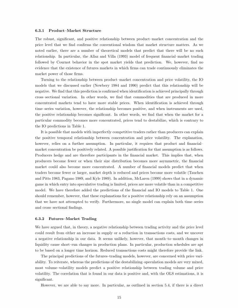
6.3.1 Product–Market Structure
The robust, significant, and positive relationship between product–market concentration and theprice level that we find confirms the conventional wisdom that market structure matters. As wenoted earlier, there are a number of theoretical models that predict that there will be no suchrelationship. In particular, the Allaz and Villa (1993) model of frequent financial–market tradingfollowed by Cournot behavior in the spot market yields that prediction. We, however, find noevidence that the existence of futures markets in which firms can trade continuously eliminates themarket power of those firms.
Turning to the relationship between product–market concentration and price volatility, the IOmodels that we discussed earlier (Newbery 1984 and 1990) predict that this relationship will benegative. We find that this prediction is confirmed when identification is achieved principally throughcross–sectional variation. In other words, we find that commodities that are produced in moreconcentrated markets tend to have more stable prices. When identification is achieved throughtime–series variation, however, the relationship becomes positive, and when instruments are used,the positive relationship becomes significant. In other words, we find that when the market for aparticular commodity becomes more concentrated, prices tend to destabilize, which is contrary tothe IO predictions in Table 1.
It is possible that models with imperfectly competitive traders rather than producers can explainthe positive temporal relationship between concentration and price volatility. The explanation,however, relies on a further assumption. In particular, it requires that product and financial–market concentration be positively related. A possible justification for that assumption is as follows.Producers hedge and are therefore participants in the financial market. This implies that, whenproducers become fewer or when their size distribution becomes more asymmetric, the financialmarket could also become more concentrated. A number of financial models predict that whentraders become fewer or larger, market depth is reduced and prices become more volatile (Tauchenand Pitts 1983, Pagano 1989, and Kyle 1989). In addition, McLaren (1999) shows that in a dynamicgame in which entry into speculative trading is limited, prices are more volatile than in a competitivemodel. We have therefore added the predictions of the financial and IO models to Table 1. Oneshould remember, however, that these explanations for a positive relationship rely on an assumptionthat we have not attempted to verify. Furthermore, no single model can explain both time–seriesand cross–sectional findings.
6.3.2 Futures–Market Trading
We have argued that, in theory, a negative relationship between trading activity and the price levelcould result from either an increase in supply or a reduction in transactions costs, and we uncovera negative relationship in our data. It seems unlikely, however, that month–to–month changes inliquidity cause short–run changes in production plans. In particular, production schedules are aptto be based on a longer time horizon. Reduced transactions costs might therefore provide the link.
The principal predictions of the futures–trading models, however, are concerned with price vari-ability. To reiterate, whereas the predictions of the destabilizing–speculation models are very mixed,most volume–volatility models predict a positive relationship between trading volume and pricevolatility. The correlation that is found in our data is positive and, with the OLS estimations, it issignificant.
However, we are able to say more. In particular, as outlined in section 5.4, if there is a direct
15

link or feedback between volume and volatility, the positive relationship should survive the use ofinstruments. If the correlation is due to a common–causal factor or latent variable, in contrast,the significance of the relationship should disappear when instruments are used. We find that thesignificance of the relationship does indeed disappear when we use instruments. This suggests thatthe link between the two is not direct and that both variables are influenced by a common factorsuch as the exogenous arrival of new information.25 Our findings are thus consistent with simplemodels, such as the Mixture of Distributions, but not with many more sophisticated theories.
7 Conclusions
To summarize, we find that traditional market–structure models in which price levels are positivelyrelated to product–market concentration perform well. In particular, we find no evidence of thecomplete unraveling that is predicted to lead to competitive pricing in commodity markets withcontinuous futures trading (e.g., Allaz and Villa 1993).
Market–structure models of price stability, in contrast, do less well. In particular, no singlemodel that we discuss can explain the existence of a negative relationship between horizontal–market concentration and price volatility that we find in the cross section coupled with a positiverelationship between those variables that we find in the time series.
Turning to financial–market activity, increased liquidity appears to be associated with lowerprices. We argue that this relationship is most likely due to a reduction in the costs of transacting.However, it could also be strategic, as in the Allaz (1992) model.
Finally, as with most empirical studies of financial markets, we find a positive relationship be-tween trading volume and price volatility in the time series. Moreover, since we deal with multiplerelated markets, we are able to assess that relationship in the cross section and we find that it isalso positive. Our findings are thus consistent with the predictions of some destabilizing–speculationand most volume–volatility models. We can, however, go further. Indeed, we are able to exploit ourinstrumental–variables technique to distinguish between broad classes of theories that predict a pos-itive relationship. When we do this, we find evidence that the link is not direct and that there is nofeedback between volume and volatility. Rather the correlation appears to be due to an unobservedvariable such as the arrival of new information that affects volume and volatility simultaneously.
25 One might wonder whether the lack of significance of the coefficients of the measures of volume is due to the useof instruments or to the correction for heteroskedastic and autocorrelated errors. Since the first–step estimates arevery similar to the second, it is clear that the lack of significance is due to the use of instruments.
16
References Cited
Admati, A.R. and Pfleiderer, P. (1988) “A Theory of Intraday Trading,” Review of Financial Stud-ies, 1: 3-40.
American Metals Market (Various years) Metal Statistics: The Statistical Guide to North AmericanMetals.
Anderson, R.W. (1991) “Futures Trading for Imperfect Cash Markets: A Survey,” in CommodityFutures and Financial Markets, L. Phlips (ed.) Kluwer, 207-248.
Anderson, R.W. and Gilbert, C.L. (1988) “Commodity Agreements and Commodity Markets: Lessonsfrom Tin,” Economic Journal, 98: 1-15.
Allaz, B. (1992) “Oligopoly, Uncertainty, and Strategic Forward Transactions,” International Jour-nal of Industrial Organization, 10: 297-308.
Allaz, B. and Villa, J-L. (1993) “Cournot Competition, Forward Markets, and Efficiency,” Journalof Economic Theory, 59: 1-16.
Bessembinder, H. and Seguin, P.J. (1993) “Price Volatility, Trading Volume, and Market Depth:Evidence from Futures Markets,” Journal of Financial and Quantitative Analysis, 28: 21-39.
Bessembinder, H., Coughenour, J.F., Seguin, P.J., and Smoller, M.M. (1995) “ Mean Reversion inEquilibrium Asset Prices: Evidence from Futures Term Structure,” Journal of Finance, 50:361-375.
Brunetti, C. and Gilbert, C.L. (1996) “Metals Price Volatility,” Resources Policy, 21: 237–254.
Carlton, D. (1986) “The Rigidity of Prices,” American Economic Review, 76: 637–658.
Clark, P.K. (1973) “A Subordinated Stochastic Process Model with Finite Variance for SpeculativePrices,” Econometrica, 41: 135-155.
Cox, C.C. (1976) “Futures Trading and Market Information,” Journal of Political Economy, 84:1215–1237.
Danthine, D.-P. (1978) “Information, Futures Prices, and Stabilizing Speculation,” Journal of Eco-nomic Theory, 17: 79–98.
Domberger, S. and Fiebig, D.G. (1993) “The Distribution of Price Changes in Oligopoly,” Journalof Industrial Economics, 41: 295–313.
Epps, T.W. and Epps, M.L. (1976) , “The Stochastic Dependence of Security Price Changes andTransactions Volumes: Implications for the Mixture–of–Distributions Hypothesis,” Economet-rica, 44: 305-321.
Figlewski, S. (1981) “Futures Trading and Volatility in the GNMA Market,” Journal of Finance,36: 445–456.
Foster, A.J. (1995) “Volume–Volatility Relationships for Crude Oil Futures Markets,” Journal ofFutures Markets, 15: 929-951.
17

Gordon–Ashworth, F. (1984) International Commodity Control, Croom, Helm, Beckworth.
Karpoff, J.M. (1987) “The Relationship Between Price Changes and Trading Volume: A Survey,”Journal of Financial and Quantitative Analysis, 22: 109-126.
Kawai, M. (1983) “Price Volatility of Storable Commodities Under Rational Expectations in Spotand Futures Markets,” International Economic Review, 24: 435–459.
Kyle, A.S. (1984) , “Market Structure, Information, Futures Markets, and Price Formation,” inInternational Agricultural Trade: Advanced Readings in Price Formation, Market Structure,and Price Instability, G. Storey, A. Schmitz, and A.H. Sarris (eds.) Boulder: Westview Press,45-64.
Kyle, A.S. (1985) , “Continuous Auctions and Insider Trading,” Econometrica, 53: 1315-1335.
Kyle, A.S. (1989) , “Informed Speculation with Imperfect Competition,” Review of Economic Stud-ies, 56: 317-356.
McLaren, J. (1999) “Speculation on Primary Commodities: The Effects of Restricted Entry,” Re-view of Economic Studies, 66: 853–871.
Newey, W.K. and West, K.D. (1987) “A Simple, Positive Semi-definite, Heteroskedasticity and Au-tocorrelation Consistent Covariance Matrix,” Econometrica, 55: 703-708.
Newbery, D.M. (1984) “Commodity Price Stabilization in Imperfect or Cartelized Markets,” Econo-metrica, 52: 563-578.
Newbery, D.M. (1987) “When Do Futures Destabilize Spot Prices?” International Economic Re-view, 28: 291–297.
Newbery, D.M. (1990) “Cartels, Storage, and the Suppression of Futures Markets,” European Eco-nomic Review, 34: 1041-1060.
Newbery, D.M. and Stiglitz, J.E. (1981) The Theory of Commodity Price Stabilization: A study inthe economics of risk. Oxford: Clarendon Press.
OECD (1999) Statistics Compendium.
Pagano, M. (1989) , “Endogenous Market Thinness and Stock Price Volatility,” Review of EconomicStudies, 56: 269-288.
Pindyck, R.S. (1999) “The Long–Run Evolution of Energy Prices,” Energy Journal, 20: 1-27.
Pinkse, J. and Slade, M.E. (2001) “Mergers, Brand Competition, and the Price of a Pint,” EuropeanEconomic Review, forthcoming.
Schmalensee, R. (1989) “Inter–Industry Studies of Structure and Performance,” in Handbook of In-dustrial Organization, R. Schmalensee and R.D. Willig (eds.) Elsevier, 951–1009.
Schwartz, E.S. (1997) “The Stochastic Behavior of Commodity Prices: Implications for Valuationand Hedging,” Journal of Finance, 52: 923-974.
Schwert, G.W. and Seguin, P.J. (1990) “Heteroskedasticity in Stock Returns,” Journal of Finance,45: 1129-1156.
18

Simpson, W. and Ireland, T. (1985) “The Impact of Financial Futures on the Cash Market for Trea-sury Bills,” Journal of Financial and Quantitative Analysis,” 30: 71–79.
Slade, M.E. (1991) “Market Structure, Marketing Method, and Price Instability,” Quarterly Journalof Economics, 106: 1309-1340.
Slade, M.E. (2001) “Managing Projects Flexibly: An Application of Real-Option Theory,” Journalof Environmental Economics and Management, 41, 193-233.
Stein, J.C. (1987) “Informational Externalities and Welfare-Reducing Speculation,” Journal of Po-litical Economy, 95: 1123–1145.
Tauchen, G.E. and Pitts, M. (1983) “The Price Variability-Volume Relationship on Speculative Mar-kets,” Econometrica, 51: 485-505.
Tauchen, G., Zhang, H., and Liu, M. (1996) “Volume, Volatility, and Leverage: A Dynamic Analy-sis,” Journal of Econometrics, 74: 177-208.
Thille, H. and Slade, M.E. (2000) “Forward Trading and Adjustment Costs in Cournot Markets,”Cahiers d’Economie Politique, 37: 177-195.
Turnovsky, S.J. (1979) “Futures Markets, Private Storage, and Price Stabilization,” Journal of Pub-lic Economics,” 12: 301–327.
Turnovsky, S.J. and Campbell, R.B. (1985) “The Stabilizing and Welfare Properties of Futures Mar-kets: A Simulation Approach,” International Economic Review, 26: 277–303.
Wang, J. (1994) “A Model of Competitive Stock Trading,” Journal of Political Economy, 102: 127-168.
Williams, J.C. (2001) “Commodity Futures and Options,” Chapter 13 in Handbook of AgriculturalEconomics, Vol. 1, B. Gardner and G Rausser (eds.) Elsevier, 746-816.
19

..........................................................................................................................................
................................................................................................................................................................................................................................................................
...............................................................
...............................................................................................................................
........................................................................................................................
.................................................................................................................................................
..............................................................................
.........................................................................................................................................................................................................................................................................................................................................................
.........................................................................................................................
.....................................................................................................................................................................................................
..................................................................................................
...................................................................................................................................................................................................................................................
..............................................................................................................
.......................................................................................................................................................................................
...................................................
...............................................................................................
.................................................................
....................................................................................................................................
..........................................................
..................................................................................
...........................................
...............................................................................................................................................................................................................
..........................................................................................................................................................
........................................................................
..............................
........................................................................................................................................
..................................
...................................
..............................................................
Figure 1: Real Spot Price, Weighted Averages
Time
$ per ton
.......................................................................................................................................................................................................................................................................................................................................................................................................................................................................................................................................................................................................................................................
......................
...........
1990 1992 1994 1996 1998
........
........
........
........
........
........
........
........
........
........
........
........
........
........
........
........
........
........
........
........
........
........
........
........
........
........
........
........
........
........
........
........
........
........
........
........
........
........
........
........
........
........
........
........
........
........
........
........
........
........
........
........
........
........
........
........
........
........
........
........
....
...........
...........
...........
...........
...........
...........
1500
2000
2500
3000
3500
4000
....................................................................................................................................................................................................................................................................................................................................................................................................................................................................................................................................................................................................................................................................................................................................................................................................................................................................................................................................................................................................................................................................................................................................................................................................................................................................................................................................................................................................................................................................................................................................................................................................................................................................................................................................................................................................................................................................................................................................................................................................................................................................................................................................................................................................................................................................................................................................................................................................................................................................................................................................................................................................................................................................................................................
..........................
........... ......
Value weightedEqually weighted
..........................................................................................................................................................................................................................................................................................................................................................................
........
........
........
........
........
........
........
........
........
........
........
........
........
........
......................................................................................................................................................................................................................................................................................................................................................................................................................................................................................................................................................................................................................................................................................................................................................................................................................................................
........
........
........
........
........
........
........
........
........
........
........
........
........
.........................................................................................................................................................................................................................
........
........
........
........
.........
........
........
........
........
........
........
........
........................................................................................................................................................................................................................................................................................................................................................
........
........
........
........
........
........
........
........
........
........
........
........
................................................................................................................................................................................................................................................................................................................................................................................
........
........
........
........
........
........
........
........
........
........
.........................................................................................................................
........
........
........
........
........
........
........
........
........
........
................................................................................................................................................................................................................................................................................................
........
........
........
........
........
........
........
........
........
........
.....................................................................................................................................................................................................
........
........
........
........
........
........
........
........
........
........
.........
........
........
........
........
........
........
........
........
...............................................................................................................................................................................................................................................................................................................................................................................................................................................................................................................................................
........
........
........
........
........
........
........
..........................................................................................................................................................................................................................................................................................
........
........
........
........
........
........
........
........
........
..............................................................................................................................................................................................................................................................................................................................................................................................................................................................................................................................................................................................................................................................................................................................................................................................................................................................................................................................................................................................
........
........
........
........
........
........
........
........
........
........
........
........
........
.......................................................................................................................................................................................
....................................................................................................................................................................................................................
........
........
........
........
........
........
........
........
........
........
........
........
........
........
........
........
........
........
........
........
........
........
..........................................................................................................................................................................................................................................................................................................................................................................................................................................................................................................................................................................................................................................................................................................................................
..................................................................................................................................
..........................................................................................................................................................................................................................................................................................................................................................................................................................................................................................................................................................................................................................................................................................
..................................................................................................................................................................................................................................................................................................................................................................................................................
...
........
...
........
...
.........................................................................................................................................................................................................................................................................................................................................................................................................................................
..........................................................................................................................................................................................................................................
..................................................................................................................
................................................................................................................................................................................................................................................................................................................................................................................................................................................................................................................................................................................................................................................................................................................................................................................................................................................................................................................................................................................................................................................................................................................................................................................................................................................................................................................................................................................................................................................................................................................................................................................................................................................................................................................................................................................................................................................................................................................................................................................................................................................................................
...........................................................................................................
...................
Figure 2: Spot-Price Volatility, Weighted Averages
Time
Percent
.......................................................................................................................................................................................................................................................................................................................................................................................................................................................................................................................................................................................................................................................
......................
...........
1990 1992 1994 1996 1998
........
........
........
........
........
........
........
........
........
........
........
........
........
........
........
........
........
........
........
........
........
........
........
........
........
........
........
........
........
........
........
........
........
........
........
........
........
........
........
........
........
........
........
........
........
........
........
........
........
........
........
........
........
........
........
........
........
........
........
........
....
...........
...........
...........
...........
...........
...........
0.005
0.010
0.015
0.020
0.025
0.030
....................................................................................................................................................................................................................................................................................................................................................................................................................................................................................................................................................................................................................................................................................................................................................................................................................................................................................................................................................................................................................................................................................................................................................................................................................................................................................................................................................................................................................................................................................................................................................................................................................................................................................................................................................................................................................................................................................................................................................................................................................................................................................................................................................................................................................................................................................................................................................................................................................................................................................................................................................................................................................................................................................................................
..........................
........... ......
Value weightedEqually weighted
20

Figure 3Distinguishing Between a Direct Link and a Common Causal Factor
1
)
PPPPPPPPPq
PPPP
PPPP
Pi
x
y1
y2
z1
z2
A
1
)
PPPPPPPPPq
PPPP
PPPP
Pi
?
6
x
y1
y2
z1
z2
B
21

Table 1: Predicted Effects of Product–Market Concentration
Type of Model Effect on Price Level
IO Cournot (1838) +Bertrand (1883) 0
Allaz (1992) +Allaz and Villa (1993) 0
Thille and Slade (2000) +
In Our Data +
Effect On Volatility
IO Newbery (1984a) -Newbery (1990) -
Through trader concentration
Financial Tauchen and Pitts (1983) +Pagano (1989) +
Kyle (1989) +IO McLaren (1999) +
In Our Data - in Cross Section+ Otherwise
22
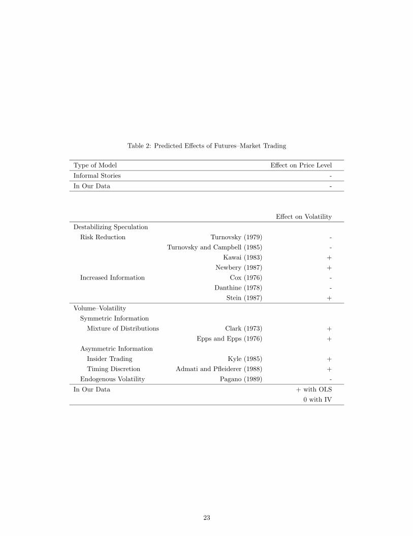
Table 2: Predicted Effects of Futures–Market Trading
Type of Model Effect on Price Level
Informal Stories -
In Our Data -
Effect on Volatility
Destabilizing SpeculationRisk Reduction Turnovsky (1979) -
Turnovsky and Campbell (1985) -Kawai (1983) +
Newbery (1987) +Increased Information Cox (1976) -
Danthine (1978) -Stein (1987) +
Volume–VolatilitySymmetric Information
Mixture of Distributions Clark (1973) +Epps and Epps (1976) +
Asymmetric InformationInsider Trading Kyle (1985) +Timing Discretion Admati and Pfleiderer (1988) +
Endogenous Volatility Pagano (1989) -
In Our Data + with OLS0 with IV
23
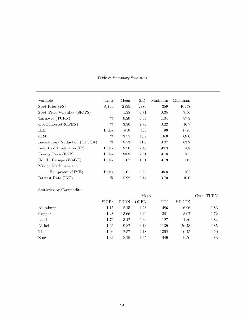
Table 3: Summary Statistics
Variable Units Mean S.D. Minimum MaximumSpot Price (PS) $/ton 2835 2386 359 10958Spot–Price Volatility (SIGPS) 1.38 0.71 0.35 7.56Turnover (TURN) % 9.29 5.64 1.04 37.3Open Interest (OPEN) % 3.36 3.76 0.22 16.7HHI Index 659 463 99 1785CR4 % 37.5 15.2 16.0 69.0Inventories/Production (STOCK) % 9.73 11.6 0.07 63.2Industrial Production (IP) Index 97.6 2.46 93.3 108Energy Price (ENP) Index 99.9 2.01 94.8 105Hourly Earnigs (WAGE) Index 107 4.01 97.9 115Mining Machinery and
Equipment (MME) Index 101 0.85 98.8 103Interest Rate (INT) % 5.92 2.14 3.70 10.0
Statistics by CommodityMean Corr. TURN
SIGPS TURN OPEN HHI STOCKAluminum 1.15 8.15 1.28 486 6.96 0.83Copper 1.48 13.66 1.69 361 3.07 0.72Lead 1.70 3.42 0.60 127 1.30 0.84Nickel 1.61 9.82 6.13 1139 26.73 0.85Tin 1.04 12.57 9.18 1392 10.75 0.90Zinc 1.33 8.15 1.25 449 9.56 0.83
24

Table 4: Price Level Equations
OLS Regressions# HHI TURN OPEN STOCK TREND IP Fixed Effectsa R2
1 0·52∗ −17·8∗ · · · −17·9∗∗ −16·3∗∗ 60·2∗∗ C 0·94(0·23) (8·7) (3·7) (4·8) (15·8)
2 0·60∗∗ −38·5∗∗ · · · −24·5∗∗ · · · 75·5 C&Y 0·95(0·22) (8·5) (3·7) (30·4)
3 1·94∗∗ · · · −177·∗∗ 0·22 −18·4∗∗ 65·2∗∗ C 0·95(0·26) (18·6) (4·0) (4·6) (14·6)
4 2·16∗∗ · · · −209·∗∗ −3·70 · · · 59·0∗ C&Y 0·96(0·24) (17·3) (3·8) (27·8)
IV Regressions# HHI TURN OPEN STOCK TREND IP Fixed Effectsa R2
1 0·21 −36·77 · · · −15·22 −13·78 60·12∗∗ C 0·94(0·35) (24·19) (9·42) (7·64) (19·03)
2 1·18∗ −152·05∗∗ · · · −54·15∗∗ · · · 96·11∗ C&Y 0·93(0·49) (38·11) (12·34) (37·55)
3 1·56∗∗ · · · −194·21∗∗ −0·68 −21·72∗∗ 52·05∗∗ C 0·95(0·49) (39·29) (10·35) (7·42) 15·80
4 2·06∗∗ · · · −244·77∗∗ −16·80 · · · 55·62∗ C&Y 0·96(0·51) (43·38) (11·72) (30·42)
a C means commodity fixed effects and Y means year fixed effects.
Standard errors in parentheses.
* denotes significance at 5%, ** denotes significance at 1%
Factor prices included but not shown.
25
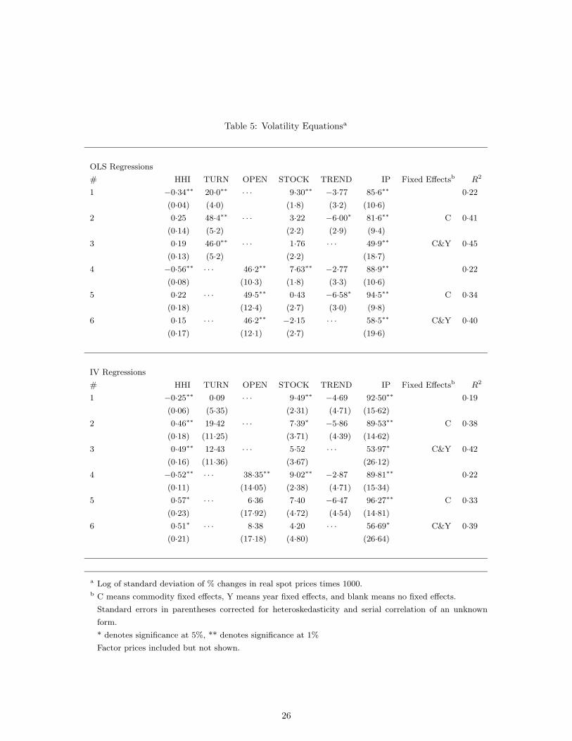
Table 5: Volatility Equationsa
OLS Regressions
# HHI TURN OPEN STOCK TREND IP Fixed Effectsb R2
1 −0·34∗∗ 20·0∗∗ · · · 9·30∗∗ −3·77 85·6∗∗ 0·22
(0·04) (4·0) (1·8) (3·2) (10·6)
2 0·25 48·4∗∗ · · · 3·22 −6·00∗ 81·6∗∗ C 0·41
(0·14) (5·2) (2·2) (2·9) (9·4)
3 0·19 46·0∗∗ · · · 1·76 · · · 49·9∗∗ C&Y 0·45
(0·13) (5·2) (2·2) (18·7)
4 −0·56∗∗ · · · 46·2∗∗ 7·63∗∗ −2·77 88·9∗∗ 0·22
(0·08) (10·3) (1·8) (3·3) (10·6)
5 0·22 · · · 49·5∗∗ 0·43 −6·58∗ 94·5∗∗ C 0·34
(0·18) (12·4) (2·7) (3·0) (9·8)
6 0·15 · · · 46·2∗∗ −2·15 · · · 58·5∗∗ C&Y 0·40
(0·17) (12·1) (2·7) (19·6)
IV Regressions
# HHI TURN OPEN STOCK TREND IP Fixed Effectsb R2
1 −0·25∗∗ 0·09 · · · 9·49∗∗ −4·69 92·50∗∗ 0·19
(0·06) (5·35) (2·31) (4·71) (15·62)
2 0·46∗∗ 19·42 · · · 7·39∗ −5·86 89·53∗∗ C 0·38
(0·18) (11·25) (3·71) (4·39) (14·62)
3 0·49∗∗ 12·43 · · · 5·52 · · · 53·97∗ C&Y 0·42
(0·16) (11·36) (3·67) (26·12)
4 −0·52∗∗ · · · 38·35∗∗ 9·02∗∗ −2·87 89·81∗∗ 0·22
(0·11) (14·05) (2·38) (4·71) (15·34)
5 0·57∗ · · · 6·36 7·40 −6·47 96·27∗∗ C 0·33
(0·23) (17·92) (4·72) (4·54) (14·81)
6 0·51∗ · · · 8·38 4·20 · · · 56·69∗ C&Y 0·39
(0·21) (17·18) (4·80) (26·64)
a Log of standard deviation of % changes in real spot prices times 1000.b C means commodity fixed effects, Y means year fixed effects, and blank means no fixed effects.
Standard errors in parentheses corrected for heteroskedasticity and serial correlation of an unknown
form.
* denotes significance at 5%, ** denotes significance at 1%
Factor prices included but not shown.
26

Appendix:
Table A: IV Regressions with a Smaller Instrument Seta
Price Level
# HHI TURN OPEN STOCK TREND IP Fixed Effectsb R2
1 0·64 −84·27∗∗ · · · −15·20 −17·62∗ 71·16∗∗ C 0·93
(0·44) (31·14) (10·66) (8·35) (21·41)
2 1·98∗∗ −248·22∗∗ · · · −59·54∗∗ · · · 105·75∗ C&Y 0·89
(0·61) (47·97) (15·33) (44·30)
3 2·47∗∗ · · · −252·72∗∗ 9·83 −18·77∗ 41·12∗ C 0·95
(0·57) (44·72) (11·39) (7·71) (17·35)
4 2·94∗∗ · · · −308·23∗∗ −7·64 · · · 44·08 C&Y 0·95
(0·59) (47·79) (13·83) (31·88)
Volatilityc
# HHI TURN OPEN STOCK TREND IP Fixed Effectsb R2
1 −0·25∗∗ −1·47 · · · 10·24∗∗ −4·32 92·44∗∗ 0·19
(0·06) (5·44) (2·41) (4·74) (15·67)
2 0·51∗∗ 14·90 · · · 9·57∗ −5·07 91·24∗∗ C 0·36
(0·18) (12·26) (4·29) (4·47) (14·81)
3 0·55∗∗ 6·00 · · · 6·93 · · · 55·14∗ C&Y 0·40
(0·17) (12·74) (4·33) (26·46)
4 −0·58∗∗ · · · 44·72∗∗ 10·32∗∗ −1·84 88·80∗∗ 0·22
(0·12) (14·69) (2·52) (4·73) (17·36)
5 0·59∗ · · · 5·84 9·40 −5·53 95·88∗∗ C 0·33
(0·24) (18·33) (5·13) (4·60) (14·86)
6 0·55∗ · · · 5·56 6·04 · · · 56·34∗ C&Y 0·39
(0·22) (17·47) (5·28) (26·71)
a Excludes silver inventories and CR4.b C means commodity fixed effects, Y means year fixed effects, and blank means no fixed effects.c Log of standard deviation of % changes in real spot prices times 1000.
Standard errors in parentheses corrected for heteroskedasticity and serial correlation of an unknown form.
* denotes significance at 5%, ** denotes significance at 1%
Factor prices included but not shown.
27
Related Documents