3 Comments About the Strengthening Mechanisms in Commercial Microalloyed Steels and Reaction Kinetics on Tempering in Low-Alloy Steels Eduardo Valencia Morales Department of Physics, Central University of Las Villas, Villa Clara Cuba 1. Introduction It is well known that hot-rolled microalloyed steels derive their overall strength from different strengthening mechanisms that simultaneously operate, such as: solid solution strengthening, hardening by the grain size refinement, precipitation strengthening and transformation induced dislocation strengthening [1]. Precipitation of fine carbonitride particles during thermomechanical processing has been used for many years to improve the mechanical properties of the microalloyed steels, where very small amounts (usually below 0.1 wt%) of strong carbide and nitride forming elements such as niobium, titanium and/or vanadium are added for grain refinement and precipitation strengthening. Both grain refinement and precipitation strengthening in microalloyed steels depend upon the formation of fine carbonitride particles, of about 10 nm or less in diameter, which may form in austenite during hot rolling, along the γ/α interface during the austenite to ferrite transformation ( interphase precipitation), or as semicoherent particles in ferrite during final cooling. Each one of these basic precipitation modes will lead to its own characteristic particle distribution, and to generally different effects on steel properties [2]. First systematic investigations on microalloyed steels were carried out in the early sixties at the University of Sheffield [3,4], including initial observations of carbonitride particles by transmission electron microscopy (TEM). According to the early literature on niobium steels yield strength contribution of about 100 MNm -2 could be obtained in the as rolled condition due to the presence of fine carbonitride particles, which were observable in the TEM [5]. Even larger contributions of up to 200 MNm -2 were reported for niobium/vanadium [6] and titanium steels [7]. In principle, these experimental results appeared to be in good agreement with theoretical predictions, based upon the Orowan-Ashby model of precipitation strengthening with carbonitride particles of about 3 nm in diameter [7,8]. The most of the early results cited above were obtained by the observation in TEM of the carbonitride particles but did not determine the origin of the observed carbonitrides [9]. It was only later that electron diffraction methods were employed to distinguish unequivocally between the three modes of carbonitride precipitation [10], and the importance of carbonitride formation in ferrite for the effectiveness of the precipitation www.intechopen.com

Welcome message from author
This document is posted to help you gain knowledge. Please leave a comment to let me know what you think about it! Share it to your friends and learn new things together.
Transcript

3
Comments About the Strengthening Mechanisms in Commercial Microalloyed
Steels and Reaction Kinetics on Tempering in Low-Alloy Steels
Eduardo Valencia Morales Department of Physics, Central University of Las Villas, Villa Clara
Cuba
1. Introduction
It is well known that hot-rolled microalloyed steels derive their overall strength from different strengthening mechanisms that simultaneously operate, such as: solid solution strengthening, hardening by the grain size refinement, precipitation strengthening and transformation induced dislocation strengthening [1]. Precipitation of fine carbonitride particles during thermomechanical processing has been used for many years to improve the mechanical properties of the microalloyed steels, where very small amounts (usually below 0.1 wt%) of strong carbide and nitride forming elements such as niobium, titanium and/or vanadium are added for grain refinement and precipitation strengthening. Both grain refinement and precipitation strengthening in microalloyed steels depend upon the formation of fine carbonitride particles, of about 10 nm or less in diameter, which may form in austenite during hot rolling, along the γ/α interface during the austenite to ferrite transformation ( interphase precipitation), or as semicoherent particles in ferrite during final cooling. Each one of these basic precipitation modes will lead to its own characteristic particle distribution, and to generally different effects on steel properties [2]. First systematic investigations on microalloyed steels were carried out in the early sixties at the University of Sheffield [3,4], including initial observations of carbonitride particles by transmission electron microscopy (TEM). According to the early literature on niobium steels yield strength contribution of about 100 MNm-2could be obtained in the as rolled condition due to the presence of fine carbonitride particles, which were observable in the TEM [5]. Even larger contributions of up to 200 MNm-2 were reported for niobium/vanadium [6] and titanium steels [7]. In principle, these experimental results appeared to be in good agreement with theoretical predictions, based upon the Orowan-Ashby model of precipitation strengthening with carbonitride particles of about 3 nm in diameter [7,8].
The most of the early results cited above were obtained by the observation in TEM of the carbonitride particles but did not determine the origin of the observed carbonitrides [9]. It was only later that electron diffraction methods were employed to distinguish unequivocally between the three modes of carbonitride precipitation [10], and the importance of carbonitride formation in ferrite for the effectiveness of the precipitation
www.intechopen.com

Alloy Steel – Properties and Use
54
strengthening mechanism was generally realized [11]. Today, most authors agree that a significant strengthening effect can only be obtained when carbonitride particles precipitate semicoherently in the ferrite phase [12], and that such precipitation will be particularly effective in the case of hot strip products where a combination of shorter rolling times, higher finishing temperatures, and rapid cooling rates after rolling should cause a larger amount of microalloying elements to remain in solution before coiling [13]. Then, a larger volume fraction of very fine particles will thus be available for a more efficient precipitation strengthening during final cooling of the coil. However, no ferrite-nucleated carbonitride particles were found in commercial Nb, NbTi and NbTiV microalloyed steels processed under industrial conditions on a hot strip mill [9, 14-16]. Besides, it was demonstrated that all precipitation strengthening will be provided by carbonitrides particles which have nucleated in austenite during finish rolling, or by interphase precipitation nucleated during the ┛┙ transformation. The contribution of dislocation strengthening has been usually neglected in these hot strip steels because of their polygonal ferrite microstructure. In this sense, relatively high dislocation densities were found in hot strip microalloyed steels with higher carbon and manganese contents, although the microstructure had remained polygonal ferrite + pearlite [15].
It should be realized that many of the results which are presented in the literature have been derived from laboratory tests and processing. The characteristic hot strip processing conditions during finish rolling (high strain rates and short interpass times), however, are difficult to simulate in the laboratory [16]. It is therefore important to study the effects of hot strip rolling in industrially processed materials in order to verify whether real results conform to generally accepted expectations.
2. Origin of carbonitrides and strengthening mechanisms in commercial hot strip microalloyed steels
2.1 Nb microalloyed steel
A first study was carried out on commercial hot strip steel where niobium was the only microalloy element with the following chemical composition: 0.07% C, 0.014% Si, 0.68% Mn, 0.035% Al, 0.04% Nb, 0.0096% N and rest of Fe [14]. The processing parameters of industrial hot strip rolling were: Soaking temperature-1150 ºC, finish rolling start temperature-1080 ºC, finish rolling end temperature-890 ºC, cooling rate-10 ºC/s, coiling temperature-650 ºC and final thickness 10 mm.
In austenite, at roughing temperature, the carbonitrides nucleate preferentially on the grain boundaries where simultaneously are occurring the recrystallization processes. During the finish rolling at low temperatures also occurs an extensive precipitation of fine carbonitrides on subgrain boundaries, suggesting that they have nucleated in deformed (unrecrystallised) austenite, although the carbonitrides can also choose the ┛-┛ boundaries as suitable places for nucleation showed in the TEM images by its aligned distribution. Figure 1a shows the extensive precipitation in austenite during the finish rolling (TEM dark field image). The diffraction pattern in this Figure indicates the position of the objective aperture which was used for the dark field illumination of carbonitrides. As can be appreciated, the position of the carbonitride reflection (showed by the aperture objective position) not obeys the Baker-Nutting orientation relationship with respect to the surrounding ferrite, Figure 1b. Thus, the
www.intechopen.com

Comments About the Strengthening Mechanisms in Commercial Microalloyed Steels and Reaction Kinetics on Tempering in Low-Alloy Steels
55
distribution of fine carbonitrides (~10 nm in diameter) decorating the previous subgrain boundaries and not obeying the Baker-Nutting orientation relationship with ferrite suggests that the above precipitation occurred in the austenite phase at finish rolling temperatures where a high plastic deformation has taken place in the microalloyed steel.
(a) (b)
Fig. 1. (a) Nb(CN) precipitation at the austenite boundary cells during last stages of the hot rolling. (b) Composite diffraction pattern of carbonitride precipitation in ferrite phase showing the nearest Baker-Nutting orientation relationship, indicating (by arrow) objetive aperture position [14].
No carbonitrides were found that could have formed from supersaturated ferrite after the phase transformation. On the other hand, clear evidence for the presence of interphase precipitation in the form of row formation (obeying only one variant of the Baker-Nutting orientation relationship) was detected on a coarse scale (not very different from the precipitation in austenite) in only two grains of the twenty grains carefully observed at TEM, Figure 2. Interphase precipitation has been associated previously with a very high strengthening potential [17,18], generating yield strengths of more than 600 MPa in a high-titanium steels after isothermal transformations [17].
Fig. 2. Interphase precipitation in Nb microalloyed steel[15].
www.intechopen.com

Alloy Steel – Properties and Use
56
A normalising treatment at 900 ºC during 30 minutes was conducted in the as coiled samples in order to verify if very fine precipitation had occurred in ferrite during coiling. In this sense, when very fine carbonitrides precipitate semicoherently in ferrite, a higher yield strength in the as rolled and coiled product is manifested, while particle coarsening and loss of particle coherence should lead to a lower yield strength after normalising. Test results indicated yield strength of 310 MPa and 312 MPa before and after the normalising treatment respectively, confirming the absence of fine scale carbonitride precipitation in ferrite during the final cooling and coiling.
According to the literature, a base value for the yield strength which includes the effects of solid solution and grain size hardening can be determined from the well-known structure-property relationship for low carbon steels, originally developed by Pickering and Gladman [19]:
1/2y fMPa 15.4 3.5 2.1 %Mn 5.4 %Si 23 %N 1.13d (1)
where the (%Mn), (%Si) and (%Nf) are the weight percentages of manganese, silicon and free nitrogen dissolved in ferrite, and d is the ferrite grain size in millimeters. The weight percent of free nitrogen that remain in solution was calculated for this microalloyed steel. It resulted to be: 0.0025% [14].
Thus, the additional contributions from dislocations and precipitation strengthening can conveniently be estimated by subtracting the base value from the total yield strength as determined by tensile testing. The results are shown in Table 1 for this Nb microalloyed steel.
Treatment of the Nb Steel
Ferrite Grain Size
(μm)
Yield Strength Calculated
(MPa)
Yield Strength Measured
(MPa)
Additional Strengthening
(MPa)
Coiled 10.0 252 310 58
Normalized 10.0 252 312 60
Table 1. Comparison between yield strength predictions from equation (1) and the results of tensile testing [14].
The results showed in Table 1 give an additional strengthening contribution of about 60 MPa. According to Gladman et al. [7], the Orowan-Ashby model of precipitation strengthening can be expressed quantitatively (in MPa) as:
1/2s 10.8f /D ln 1630D (2)
where represent the precipitation strengthening increment in MPa, f is the precipitate volume fraction and D the mean particle diameter in micrometers. The application of equation (2) to the austenite precipitation gave as result an additional strengthening
www.intechopen.com

Comments About the Strengthening Mechanisms in Commercial Microalloyed Steels and Reaction Kinetics on Tempering in Low-Alloy Steels
57
increment of about 65 MPa. This value seems to agree with the above difference between the measured and calculated yield strength. Quantitative estimates from several grains where the foil thickness has been measured by counting the number of grain boundary fringes under two-beam contrast conditions indicated an average dislocation density of about 108 cm-2 for this Nb microalloyed steel. According to the early literature [20], dislocation strengthening can be quantified by:
1/2m b (3)
where is the dislocation contribution to yield strength, m the appropriate Taylor factor for polycrystals, ┙ a geometrical factor that depends upon the type of dislocation interaction, μ the shear modulus (82,300 MPa for ferrite), b the dislocation Burgers vector (0.25 nm in ferrite), and the measured dislocation density. A value of m┙= 0.38 has been determined experimentally for pure iron [21]. Alternatively, theoretical values of m= 2.733 for bcc crystals [22] and of ┙=1/2 for dislocation forest cutting [23] would give a slightly higher estimate of m┙=0.435. Selecting m┙=0.4 as an intermediate value [15], a dislocation density of 108 cm-2 would contribute with 8 MPa to the strength of the Nb microalloyed steel, which would be considered negligible. As the interphase precipitation has only occurred in a very small fraction of the grains (two of the twenty) and in a coarse scale, their influence on the yield strength is also negligible [14].
2.2 NbTi microalloyed steel
New results were obtained from another commercial NbTi microalloyed hot strip steel [15], which reached a yield strength of 534 MPa and, according to expectations, lost part of that strength during normalizing. A Nb steel, (above referred) which only reached 310 MPa and maintained that strength after normalizing, was used as a reference material. Chemical compositions and industrial processing conditions of this NbTi steel are shown in Tables 2 and 3. Part of the material was normalized at 900 ºC for 30 minutes. Optical and electron microscopy were used to study the microstructure, and yield strength values before and after normalizing were determined as the average of five tensile tests.
Steel C Mn Si P S Al Nb Ti N
NbTi 0.12 1.21 0.33 0.023 0.008 0.048 0.057 0.059 0.008
Table 2. Chemical Composition of Hot Strip NbTi Steel in Weight Percent [15]
Steel Soaking Temperature
Finish Rolling Start End
Cooling Rate
Coiling Temperature
Final Thicknees
NbTi 1150 ºC 1079 ºC 870 ºC 10 ºC/s 650 ºC 7 mm
Table 3. Processing Parameters of Industrial Hot Strip Rolling [15]
www.intechopen.com
Alloy Steel – Properties and Use
58
The NbTi steel exhibited the smaller ferrite grain size than the Nb steel, presumably due to its higher carbon and manganese contents, which should have decreased the transformation temperature. Quantitative metallography, yield strength measurements, and structure-property relationships were used for a quantitative estimate of different strengthening contributions [15]. To begin with, the well-known empirical equation (1) served to calculate the contributions from chemical composition and ferrite grain size. Yield strength predictions from Eq. (1) are compared to tensile test results in Table 4. The difference between calculated and measured strength is usually attributed to some additional strengthening mechanism such as carbonitride precipitation or substructure strengthening. The important point in Table 4 is the very large additional strengthening of 177 MPa in the case of the NbTi steel, which was reduced to 69 MPa after normalizing [15]. As mentioned previously, normalizing did not reduce the yield strength of the Nb steel, and the additional strengthening contribution in this steel remained at around 60 MPa, a level very close to the 69 MPa exhibited by the NbTi steel after normalizing.
Treatment of the NbTi Steel
Ferrite Grain Size (μm)
Yield Strength Calculated (MPa)
Yield Strength Measured (MPa)
Additional Strengthening (MPa)
Coiled 5.0 367 534 177
Normalized 5.5 357 426 69
Table 4. Comparison between yield strength predictions from equation (1) and the results of tensile testing, [15].
Fine carbonitride precipitation was identified in all of the observed grains (twenty) at TEM, but orientation relationships determined from electron diffraction showed that these particles had nucleated in austenite [15]. In addition, carbonitride distributions appeared to be very similar to the distributions observed in a previous investigated steel [9]. In that case, quantitative metallography and the application of the Orowan–Ashby model of precipitation strengthening had indicated a strengthening contribution of about 60 to 80 MPa for carbonitride particles formed in austenite, in good agreement with the additional strengthening shown in Table 1 for the Nb steel and also for the NbTi steel after normalizing, as it is shown in Table 4.
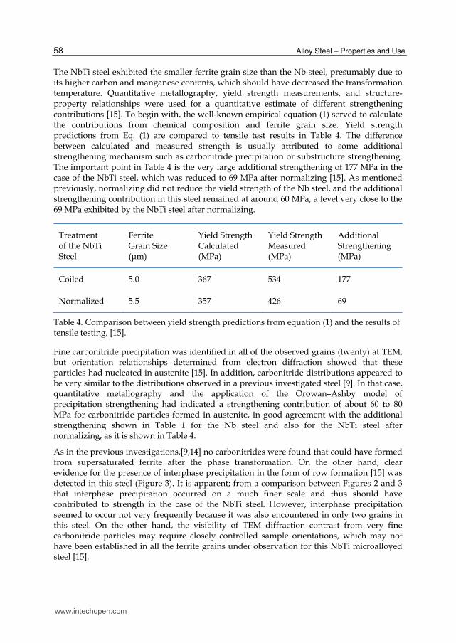
As in the previous investigations,[9,14] no carbonitrides were found that could have formed from supersaturated ferrite after the phase transformation. On the other hand, clear evidence for the presence of interphase precipitation in the form of row formation [15] was detected in this steel (Figure 3). It is apparent; from a comparison between Figures 2 and 3 that interphase precipitation occurred on a much finer scale and thus should have contributed to strength in the case of the NbTi steel. However, interphase precipitation seemed to occur not very frequently because it was also encountered in only two grains in this steel. On the other hand, the visibility of TEM diffraction contrast from very fine carbonitride particles may require closely controlled sample orientations, which may not have been established in all the ferrite grains under observation for this NbTi microalloyed steel [15].
www.intechopen.com
Comments About the Strengthening Mechanisms in Commercial Microalloyed Steels and Reaction Kinetics on Tempering in Low-Alloy Steels
59
Fig. 3. Interphase precipitation in microalloyed steel[15].
As a first approximation, if it is assumed that about one-half of the total microalloy addition would be available for fine-scale carbonitride precipitation during thermo-mechanical processing [9,15] and applying the Orowan–Ashby model, a maximum strengthening contribution of 195 MPa could be predicted for the interphase precipitation of the NbTi steel shown in Figure 3, based upon a particle size of 2.0 nm and a volume fraction of 8x10⁻⁴. If interphase precipitation had occurred in only 25 pct of the ferrite grains, a simple rule of mixtures would thus suggest a strengthening contribution of about 50 MPa in the case of the NbTi steel [15].
Another strengthening contribution could come from the presence of dislocations. In fact, dislocation densities were always higher in the NbTi steel, which again can be explained by its lower transformation temperature in comparison with the Nb steel. Quantitative estimates from several grains where the foil thickness had been measured by counting the number of grain boundary fringes under two-beam contrast conditions indicated an average dislocation density of 5x109 cm-2 for the NbTi steel [15]. Such numbers are in reasonable agreement with previous measurements of dislocation densities in microalloyed steels [24] and confirm the possibility of a transformation-induced dislocation substructure even in the case of polygonal ferrite grains.
According to Eq. (3), a strengthening contribution of 58 MPa due to the dislocation substructure of the NbTi microalloyed steel was obtained. Thus, in the case of the NbTi steel, the individual strengthening contributions from general precipitation in austenite (~70 MPa), localized interphase precipitation (~50 MPa), and dislocation substructure (~60 MPa) would add to a total of 180 MPa, a value which compares very favorably with the additional strengthening contribution found for the NbTi steel [15] in Table 4. During normalising, coarsening of fine interphase precipitate distributions and elimination of the dislocation substructure (which would not form again during air cooling due to a higher transformation temperature) can be expected to reduce the strengthening level to the contribution of austenite precipitation alone (69 MPa according to Table 4). This later strengthening contribution should survive the effect of normalizing because the formation of carbonitride particles during finish rolling occurs within the range of typical normalizing temperatures [15]. In the case of the previous Nb steel, a higher transformation temperature before coiling would leave the carbonitride precipitation in austenite as the only strengthening mechanism before and after normalizing.
www.intechopen.com

Alloy Steel – Properties and Use
60
2.3 Another NbTi and NbTiV microalloyed steels
Strength and microstructures of three new commercial microalloyed steels were investigated as a function of their chemical compositions. They were compared with the above two microalloyed steels [16]. As a common feature, all five steels had been hot rolled under similar thermomechanical processing conditions on an industrial hot strip mill, and each of them exhibited a polygonal ferrite+ pearlite microstructure. In contrast, carbon and manganese contents ranged from 0.05 wt.% to 0.14 wt.% C and from 0.5 wt % to 1.5 wt.% Mn, respectively, and microalloyed additions included pure Nb, Nb-Ti, and Nb-Ti-V combinations. Chemical compositions are shown in Table 5, together with maximum total volume fractions (Vf max) for carbonitride precipitation which were calculated assuming appropriated lattice parameters of 0.445, 0.430 and 0.415 nm for the fcc unit cell of niobium, titanium and vanadium carbonitrides, respectively [16].
Steel C Mn Si P S Al Nb Ti V N Vf max
Nb 0.07 0.68 0.01 0.012 0.009 0.04 0.04 - - 0.009 0.00045
NbTi-1 0.05 0.55 0.02 n.d. n.d. 0.02 0.02 0.06 - 0.006 0.00131
NbTi-2 0.12 1.21 0.33 0.023 0.008 0.048 0.057 0.059 - 0.008 0.00166
NbTi-3 0.11 1.54 0.28 0.026 0.007 0.01 0.04 0.11 - n.d. 0.00261
NbTiV 0.14 1.38 0.25 0.018 0.007 0.07 0.04 0.04 0.03 0.008 0.00174
Table 5. Steel compositions (wt %) and maximum total volume fraction for carbonitride precipitation [16].
Thermomechanical processing conditions are given in Table 6, confirming rather similar processing parameters for all the steels, with the exception of steel NbTiV which was rolled to smaller thickness of 3 mm. The last column in Table 6 shows the yield strength after coiling. Two distinct strength levels can be recognized: Low yield strength values in the range of 300 MPa for steels Nb and NbTi-1, and significantly higher yield strength values in the range of 500 to 600 MPa for steels NbTi-2, NbTi-3 and NbTiV [16].
Steel Soaking
/°C Roughing
/°C
Finishing
/°C
Cooling
/°C*min-1Coiling
/°C
Thickness
/mm
Y. S.
MPa
Nb 1150 ≥1080 890 10 650 10 310
NbTi-1 1230 ≥1100 870 20 630 8 332
NbTi-2 1150 ≥1070 870 10 650 7 534
NbTi-3 1225 ≥1100 895 10 650 8 638
NbTiV 1225 ≥1100 895 10 670 3 599
Table 6. Thermomechanical processing conditions and yield strength after coiling [16].
As it is shown in [16], all steels had transformed to polygonal ferrite+ pearlite. The ferrite grain size decreased from about 10 µm (average diameter) for low strength alloys Nb and NbTi-1, to 5 µm and below for high strength steels NbTi-2, NbTi-3 and NbTiV. Such grain refinement can be related to lower transformation temperatures caused by larger carbon and manganese additions to higher strength materials. Table 7 shows the additional contributions from dislocations and precipitation strengthening by subtracting the base
www.intechopen.com

Comments About the Strengthening Mechanisms in Commercial Microalloyed Steels and Reaction Kinetics on Tempering in Low-Alloy Steels
61
value obtained by Eq. (1) from the total yield strength as determined by tensile testing[16]. The results showed in Table 7, ranging from low additional strengthening contributions below 100 MPa for steels Nb and NbTi-1 to much larger additional strengthening contributions between 150 and 250 MPa for steels NbTi-2, NbTi-3 and NbTiV.
Very low dislocations densities were found in the low strength alloy, with quantitative estimates remaining at about 108 cm-2 which would be typical value for well annealed ferrite steel. On the other hand, distinctly higher dislocation densities in the range of 109 to 1010 cm-2 were encountered in the high strength steels [16]. Such an increase in dislocation density may also be related to lower transformation temperatures, and a sizeable contribution to yield strength may thus be expected to come from transformation-induced dislocations even in the case of polygonal ferrite microstructures. According to the Keh equation [15, 25], this contribution could reach about 50 MPa for dislocation densities in the range of 5x109 cm-2.
In the above steels, two different modes of fine carbonitride precipitation were detected in the as-coiled samples: Precipitation on the deformation-induced dislocation substructure in austenite, and interphase precipitation where carbonitrides had nucleated on the ┛┙ interface during transformation. Carbonitride precipitation in austenite was identified by electron diffraction and was found to be present in all the grains investigated. Mean particle diameters were observed to increase in proportion with the maximum theoretical precipitate volume fraction [16].
Steel Grain Size (µm) (MPa) ( MPa
Nb 10.0 252 58
NbTi-1 9.4 254 78
NbTi-2 5.0 367 167
NbTi-3 4.2 393 245
NbTiV 3.3 421 178
Table 7. Calculation of base yield strength, , and of additional strengthening from dislocations and precipitation, [16].
Interphase precipitation was detected in only a small number of grains, but in most of these observations was recognized through row formation. This mode of carbonitride precipitation may have occurred in other grains as well. Preliminary measurements indicated that mean particle diameters of about 2 nm were associated with the smaller sheet spacing, but reached 5 nm in other samples where the sheet spacing were larger. On one occasion, both larger and smaller sheet spacings were present in the same ferrite grain which probably had transformed during cooling through an extended temperature interval [16]. Quantitative estimates of interphase particles volume fraction gave 3.5x10⁻⁴ in NbTi-2 steel, 4.9x10⁻⁴ in Nb steel, and 7.8x10⁻⁴ in NbTi-3 steel [16].
An Orowan-Ashby analysis showed strengthening contributions of about 60 to 100 MPa from particle volume fractions in austenite in the range of 10-4 as a function of the particle diameter [16]. Local strengthening contributions from practical interphase precipitation phenomena would reach 110 to 180 MPa. But it must be remembered that interphase
www.intechopen.com
Alloy Steel – Properties and Use
62
precipitation does not seem to occur in all the ferrite grains, so that its effective contribution would be reduced through some sort of rule of mixture. It thus appears that carbonitrides nucleated in austenite do make a sizeable contribution to the steel’s yield strength [16].
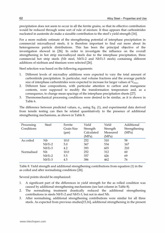
For a more realistic estimate of the strengthening potential of interphase precipitation in commercial microalloyed steels, it is therefore important to find out more about its heterogeneous particle distributions. This has been the principal objective of the investigation showed in [26]. In order to investigate the influence on the overall strengthening in hot strip microalloyed steels due to the interphase precipitation, three commercial hot strip steels (Nb steel, NbTi-2 and NbTi-3 steels) containing different additions of niobium and titanium were selected [26].
Steel selection was based on the following arguments:
1. Different levels of microalloy additions were expected to vary the total amount of carbonitride precipitation. In particular, real volume fractions and the average particle size of interphase carbonitrides were expected to increase for larger values of Vfmax.
2. Different base compositions, with particular attention to carbon and manganese contents, were supposed to modify the transformation temperature and, as a consequence, to change mean spacings of the interphase precipitation sheets [27].
3. Thermomechanical processing conditions were desired to be similar, as it is shown in Table 6.
The difference between predicted values, y, using Eq. (1), and experimental data derived from tensile testing can then be related quantitatively to the presence of additional strengthening mechanisms, as shown in Table 8.
Processing Conditions
Steel Ferrite Grain Size (μm)
Yield Strength Calculated (MPa)
Yield Strength Measured (MPa)
Additional Strengthening (MPa)
As coiled Nb 10.0 252 310 58 NbTi-2
NbTi-3 5.0 4.2
367 393
534 603
167 210
Normalised Nb NbTi-2
10.0 5.5
252 357
312 426
60 69
NbTi-3 4.5 386 462 76
Table 8. Yield strength and additional strengthening contributions from equation (1) in the as coiled and after normalising conditions [26].
Several points should be emphasized:
1. A significant part of the differences in yield strength for the as rolled condition was caused by additional strengthening mechanisms (see last column in Table 8).
2. The normalising treatment drastically reduced the additional strengthening contributions in steels NbTi-2 and NbTi-3, but not in steel Nb.
3. After normalising, additional strengthening contributions were similar for all three steels. As expected from previous studies[15,16], additional strengthening in the present
www.intechopen.com
Comments About the Strengthening Mechanisms in Commercial Microalloyed Steels and Reaction Kinetics on Tempering in Low-Alloy Steels
63
case should have come from carbonitride particles nucleated in austenite, carbonitride particles formed by interphase precipitation, and from dislocations introduced by the ┛→┙ transformation [26].
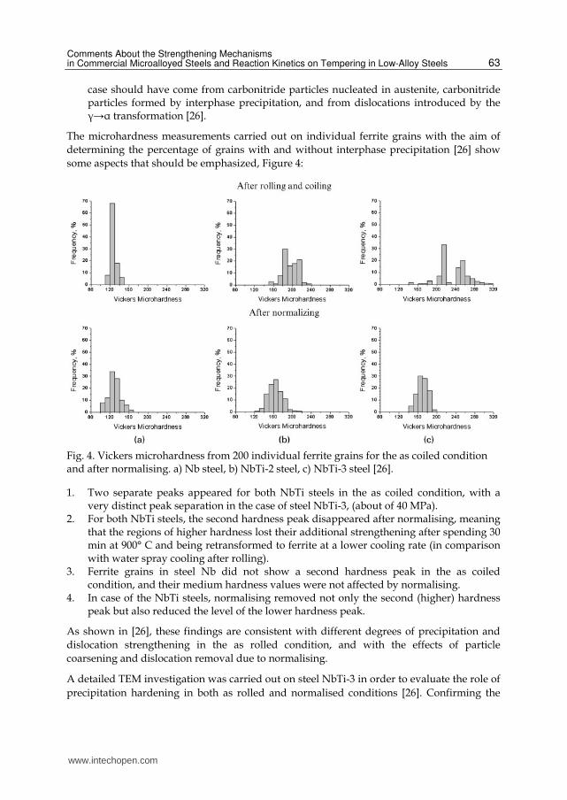
The microhardness measurements carried out on individual ferrite grains with the aim of determining the percentage of grains with and without interphase precipitation [26] show some aspects that should be emphasized, Figure 4:
Fig. 4. Vickers microhardness from 200 individual ferrite grains for the as coiled condition and after normalising. a) Nb steel, b) NbTi-2 steel, c) NbTi-3 steel [26].
1. Two separate peaks appeared for both NbTi steels in the as coiled condition, with a very distinct peak separation in the case of steel NbTi-3, (about of 40 MPa).
2. For both NbTi steels, the second hardness peak disappeared after normalising, meaning that the regions of higher hardness lost their additional strengthening after spending 30 min at 900° C and being retransformed to ferrite at a lower cooling rate (in comparison with water spray cooling after rolling).
3. Ferrite grains in steel Nb did not show a second hardness peak in the as coiled condition, and their medium hardness values were not affected by normalising.
4. In case of the NbTi steels, normalising removed not only the second (higher) hardness peak but also reduced the level of the lower hardness peak.
As shown in [26], these findings are consistent with different degrees of precipitation and dislocation strengthening in the as rolled condition, and with the effects of particle coarsening and dislocation removal due to normalising.
A detailed TEM investigation was carried out on steel NbTi-3 in order to evaluate the role of precipitation hardening in both as rolled and normalised conditions [26]. Confirming the
www.intechopen.com

Alloy Steel – Properties and Use
64
results of our previous studies on commercial hot strip steels [9, 15, 16], all fine carbonitride particles had either formed in austenite during rolling or on ┛/┙ phase boundaries during transformation. No additional carbonitride populations were found that could have formed in supersaturated ferrite, despite the unusually large microalloy addition of 0.04%Nb + 0.11%Ti. On the other hand, interphase carbonitrides were relatively large and observed frequently, indicating that a substantial fraction of the microalloy addition had remained in solution at the time of transformation. Furthermore, some form of austenite precipitation was encountered in all the ferrite grains that were investigated. Interphase precipitation was present in only some of the ferrite grains. Occasionally, grains were found to be covered completely by carbonitrides in a row formation. On other occasions, interphase precipitation would occupy only parts of a particular ferrite grain. The presence of interphase precipitation in only part of a given ferrite grain must therefore be accepted as a real phenomenon [26].
During a TEM study of a large number of grains, of which more than a hundred exhibited interphase precipitation, it was found that random particle distributions were dominant only when thin foils had been prepared parallel to the rolling plane, while row formation was encountered very frequently in longitudinal and transverse sections. Such observations can only be explained by a preferred alignment of the interphase precipitation sheets parallel to the rolling plane.
As a result of this detailed analysis, interphase precipitation was identified in 27 out of a total of 51 ferrite grains that were investigated. Thus, about one half of the grains in steel NbTi-3 should have been strengthened by interphase precipitation [26].
The effects of normalising on the mechanical properties as shown in Table 8, suggest that important changes occurred during this heat treatment with respect to precipitation and/or dislocation hardening. The first important observation, therefore, was that many carbonitrides continued to decorate typical deformation subgrain structures. It can thus be concluded that the normalising treatment did not have a major effect on carbonitride distributions that had been formed in austenite, although the average particle size was increased. The second important observation was that row formation could no longer be detected after normalising. This means that extensive particle coarsening must have occurred during normalising, including the transfer of microalloy atoms from dissolving particles in one of the original interphase precipitation sheets to growing particles located in another sheet [26]. Another important result of normalising was the reduction in dislocation density.
Quantification of local strengthening contributions in the NbTi-3 steel showed two aspects that should be emphasised in those grains strengthened by both austenite and interphase precipitation, Table 9. First, the total carbonitride volume fraction after normalising (13.0x10-
4) was not very far from the combined volume fraction of austenite +interphase precipitation after coiling (6.2 + 5.0=11.2x10⁻⁴), confirming the previous interpretation that, after normalising should have included the coarsened interphase particles. Second, the total level of precipitation strengthening for the as rolled and coiled condition was calculated by using a new average particle size (5.2 nm) determined for both the austenite and interphase precipitate populations [26].
www.intechopen.com

Comments About the Strengthening Mechanisms in Commercial Microalloyed Steels and Reaction Kinetics on Tempering in Low-Alloy Steels
65
Sample
condition
Precipitation strengthening from Eq. (2) Dislocation hardening from Eq(3)
Particle origin D, nm fx10-4 , MPa , cm-2 , MPa
As rolled
after coiling
Austenite 7.2 6.2 92 5.2x10⁹ 64
Interphase 4.0 5.0 112
Total 5.2 11.2 145
After
normalising
Austenite 12.0 6.9 70 108 <10
Total 11.0 13.0 102
Table 9. Substructural strengthening contributions in steel NbTi-3 [26].
It can be seen from Table 9, that the largest individual contribution was associated with the interphase precipitation mode, yielding average values of 112 MPa, against 92 MPa for carbonitride precipitation in austenite and 64 MPa for dislocation hardening. For
the overall strength of the steel, it is claimed in [26] that the interphase precipitation should be less effective, because it occurs only in some fraction of the ferrite grains. In addition, moving dislocations do not distinguish between the origin of the carbonitride obstacles that have to be overcome by Orowan bowing. In the presence of other carbonitride particles nucleated in austenite, therefore, the total contribution of precipitation strengthening will not amount to 92+112=204 MPa but to only 145 MPa as shown in Table 9. As a result, the local contribution of interphase precipitation to the strength of those particular ferrite grains (about 50% in steel NbTi-3) would only be 112(145/204)=79.5 MPa, against a local contribution of 92 (145/204)=65.5 MPa from austenite precipitation in the same ferrite grains [26].
Accepting the idea that austenite precipitation during rolling and dislocation generation during transformation occurred throughout the material whereas interphase precipitation was present in only 50% of the ferrite grains, considering, in addition, that precipitation and dislocation hardening would act independently and adopting a simple rule of mixture for the effects of grains with and without interphase precipitation, the final contributions of the additional ‘substructural’ mechanisms to the yield strength of steel NbTi-3 may be written (see Table 9) as y=0.5(92+64)+ 0.5(145+64)=182.5 MPa, in reasonable agreement with the additional strengthening of 210 MPa derived from tensile testing and the generally accepted structure–property relationship (Eq. (1)) [26] (see Table 8). Following the same lines of argument [26], we would expect steel NbTi-3 to reach an additional ‘substructural’ strengthening contribution of y=92+64=156 MPa without interphase precipitation. The difference, of only 182.5-156=26.5 MPa, would indicate a rather modest contribution of the interphase precipitation mode to the strength of steel NbTi-3.
Microhardness measurements can be used in principle to detect additional strengthening mechanisms which operate in only part of the ferrite grains. In this sense, it is shown in [26] that for an estimated peak separation of 40 HV (Figure 4), the additional strengthening mechanism in 53% of the ferrite grains would have contributed with an average of 99 MPa, a number that is not very far from the 79.5 MPa contribution of interphase precipitation strengthening derived from the TEM observations.
www.intechopen.com

Alloy Steel – Properties and Use
66
3. New kinetic approaches applied to reactions during tempering in low-alloy steels
3.1 Isothermal tempering
3.1.1 Introduction
The precipitation reactions which occur on tempering of low-alloy steels may all be classified as nucleation and growth transformations [28]. Extensive studies have been carried out to understand and to model the mechanisms that take place during the tempering of steels. Although it is well accepted that models based on physical principles rather than empirical data fitting give a better understanding of the individual mechanisms which occur on tempering, these models do not contemplate the complexity with which the reactions proceed in each situation T-t. In this sense, many models do not consider the overlapping of precipitation processes of different chemical natures [29, 30], and when they are taken into account, specific nucleation rates are assessed to fit the entire experimental data without considering the change that the nucleation rate could have during the progress of the reaction [31]. Another situation that commonly occurs when fitting the models, such as Johnson-Mehl-Avrami- Kolmogorov (JMAK)-like models, to the entire curve of the fraction transformed (ξ(t)) vs. lnt, is to discard the experimental uncertainties in the determination of the fraction transformed [31, 32]. Fitting such models to the entire experimental curve of the fraction transformed could therefore, in certain circumstances result in the prediction of unrealistic kinetic parameters [33].
In other works some attempts have been made [34-37] to deconvolute such experimental master curves into components due to individual processes, but it is difficult to see whether some of these fitting parameters have any physical meaning.
Recently, a general modular model for both isothermal and isochronal kinetics of phase transformations in solid state has been published [38, 39]. This model incorporates a choice of nucleation (nucleation of mixed nature) and growth mechanisms, as well as impingement. Also, the JMAK formulation has been deeply modified to suit isochronal case [40-42], but these analytical approaches need of the nucleation protocols in order to provide a suitable description of phase transformation kinetics during both isothermal and isochronal heat treatments.
In the following, an overview is given about the kinetic theory of overlapping phase transformations (KTOPT) [43] which is based on the Avrami model. This new approach permits the determination of the kinetic parameters (n, k) for simultaneous diffusion-controlled precipitation reactions based on the knowledge of a specific macroscopic parameter P(t), chosen to study the ongoing reaction. The present approach does not need to assume nucleation and growth protocols in its formulation to fit the experimental data. This new approach [43] has the particularity of calculating the kinetic parameters in defined work intervals of the fraction transformed curve rather than for the entire curve where the overlapping effect is present. Furthermore, these work intervals are distant from the boundary points ξ=0 and ξ=1in order to minimize the errors [44].
3.1.2 Fundamentals of the kinetic theory of two overlapping processes
In the kinetic theory for two overlapping precipitation processes [43] (in isothermal regime), the real fraction transformed is defined in function of the macroscopic parameter P(t) as:
www.intechopen.com

Comments About the Strengthening Mechanisms in Commercial Microalloyed Steels and Reaction Kinetics on Tempering in Low-Alloy Steels
67
1
( )( )
( )rend
P tt
P t (4)
where tend1 is the time to complete of the first process. tend1 is chosen instead of tend2 because we thus take into account the effect of the first process during the time interval t < tend1 when there is appreciable influence of the second process on the experimental parameter.
It is considered that variations of P(t) associated with each process are independent:
1 2( ) ( ) ( )P t P t P t (5)
then, the real fraction transformed is written as:
1 2
1 1 2 1
( ) ( )( )
( ) ( )rend end
P t P tt
P t P t (6)
As the fraction transformed associated which each elementary process obeys a JMAK kinetic equation, Eq. (6) can be written:
1 2
2 1
( ) ( )( )
1 ( )p
rp end
t tt
t
(7)
where
2 2
1 1
( )( )
endp
end
P t
P t (8)
The magnitude of 2(tend1) measures the degree of overlap (large or small) of the processes. Depending on the choice of P(t), the parameter p may be either positive or negative. When the variation of this parameter, with time, for one of the precipitation processes increases while for the other it decreases p<0 but when P(t) changes in the same sense, p>0.
The experimental determination of r(t) would be possible if we would be able to measure the parameter P(t) from the beginning of the phase transformations (in an isothermal regime). However, the sample takes a certain time to reach the temperature of the isothermal treatment. During this small time interval, the sample is already undergoing heat treatment, so the beginning of the transformations may be prior to that of temperature stabilization corresponding to the isothermal regime, and therefore; the real initiation of the precipitation processes is unknown.
Let us consider two processes that proceed in the same sense during the isothermal treatment (p >0) [33]. Thus, it is necessary to begin the study not from the origin of the data obtained from the measuring equipment but from the moment of time when the isothermal regime is reached. If we take the length of the sample as the macroscopic parameter, then l’(0) will be the initial length of the sample (l’(0)= l(t0)) [43]. Thus, we may compute the fraction transformed by:
1 1
'( ') '(0) ( ) (0)( )
'( ' ) '(0) ( ) (0)end end
p t p l t lt
p t p l t l (9)
www.intechopen.com

Alloy Steel – Properties and Use
68
Since r(t) cannot be obtained directly from experiment (we do not known the actual origin in time of the transformations), a relation between the fraction transformed ’(t’), (that is experimentally measurable) and r(t) is found:
0
0 0
( ) ( )( ) ( )
1 ( ) 1 ( )r r
r r
t tt t
t t
(10)
and a general expression correlating ’(t’) with the fractions transformed for the individual processes (obeying a JMAK expression) is obtained:
0 2 1 1 1 2 2( )
(1 ( ))(1 ( )) ( ) ( )lnr l end l
d tt t n n
d t
(11)
where
11(ln ln )
1( ) (1 )ln(1 )d
d
(12)
Our approach focusses on the behavior of the function Z(ξ) vs. ξ [33, 43]. This function is not symmetrical with reference to its maximum at ξ=0.632. It increases as ξ increase initially, but when ξ→1 it decreases very rapidly. By contrast Z(ξ) is nearly constant for values of ξ in the neighborhood of the point where this function is a maximum. In other words, we have an interval where ξ takes values (far from the boundary points ξ=0 and ξ=1) for which Z(ξ) depends weakly on ξ. If we allow time intervals where ξ1 (t) and ξ2(t) lie far enough from the boundary points ξ=0 and ξ=1, then we may consider that Z(ξ1) and Z(ξ2) are nearly constants.
In order to develop the equations for calculating the kinetic parameters for both processes, it should be kept in mind that ┙
l>0, (processes that progress in the same sense). Thus,
considering the definition of the fraction transformed, Eq.(9), the ξ’(t’)>1 for t′>t′end1. For the time interval (t′>t′end1), the second process (obeying a JMAK-type relation) develops alone, and therefore; the fraction transformed ξ’ (t’) should be normalized as:
2
2
'( ') '( ' )''( ) p ' t ' W
1 '( ' )end
end
t tt
t
(13)
where at t’=t’end1 the ’(t’end1)=’’(t’end1)=1 and for t’=t’end2, ’’(t’end2)=0.
According to reasoning followed in [33], for times t’end1<t’<t’end2, the second process develops alone in this time interval, therefore ξ2’(t’) increases while ξ’’(t’) decreases (for the case where ┙
l>0). Thus, it is possible to find a time interval [t
┙’, t
┚’] where the points
[ ( ''( ')), ''( ')Z t t )] and [ 2 2( '( ')), '( '))t t ] are symmetrically located about the maximum of
the Z(ξ) function (stability region). This enables to consider that 2( '( ')) ( ''( '))t t for the
above time interval and Eq.(11) can be written as:
www.intechopen.com

Comments About the Strengthening Mechanisms in Commercial Microalloyed Steels and Reaction Kinetics on Tempering in Low-Alloy Steels
69
0 2 1 2 2 2( )
(1 ( ))(1 ( )) ( ') ( '')lnr l end l l
d tt t n n
d t
(14)
or:
''( ')
( ''( '))ln '
d tN t
d t
with 2
r 0 2 1(1- ( ))(1 ( )l
l end
p nN
t t
(15)
In the above time interval, the experimental fraction transformed ’’(t’) follows a nearly
JMAK behaviour, where the N value is obtained by linear fitting of the 1
ln ln1 '' vs. lnt’
for the time interval considered.
By considering the kinetics of a second process (t’>t’end1) one may obtain 2’(t’) (or 2(t)) and the corresponding parameters n2 and k2. In this sense Eqs. (7), (10) and Eq. (15) are considered, thus it is obtained:
22 2 2 1( ) ( ) [ '( ') 1] '( ' )end
nt t p t t
N (16)
as for t’=t’end2, the 2’(t’end2)=1, and taking into account the Eq. (13) we obtain:
22 2 2( ) ( ) [ ''( ') ''( ' ) 1end
nt t t t
N (17)
For computing the kinetics of a first process (1’(t’)) at 0<t’<t’end1, Eqs.(16) and (10) are considered, thus the following expression results:
1 1 0 2 1 0 2 1 2( ) ( ) ( )[1 ( )][1 ' ( ' )] ( )[1 ' ( ' )] ' ( ')r l end r l end lt t t t t t t t (18)
We consider two situations of overlapping for the processes [33, 43].
3.1.2.1 Small overlap
A second process occurs, but it manifests itself only weakly during the interval t0<t<tend1(0<t’<t’end1); i.e., 2(tend1) is small so, the second process disturbs the first one. In this case [43]:
11 1( ) ( ) 1 [ '( ') 1]
nt t t
n (19)
where it is assumed that 2(tend1)- 2(t) 0.
3.1.2.2 Large overlap
In this case a second process is manifested strongly during the time when the first one is occurring (t0<t<tend1). As already remarked, it is necessary to pick a time interval such that 2’(t’) >0.25, i.e., Z(2’) is nearly constant and, consequently, 1’(t’) and ’(t’) are below 0.9. Therefore for times far from the boundary points ’=0 and ’=1, the Z(1’)Z(2’)Z(’)constant and Eq.(11) simplifies to:
www.intechopen.com

Alloy Steel – Properties and Use
70
( )
( )ln
d tn
d t
with 1 2
r 0 2 1(1- ( ))(1 ( ))l
l end
n nn
t t
(20)
and according to Eqs.(15) and (20); Eq.(18) reduces to:
1 11 1 2 1 2
2
( ) ( ) 1 [ '( ') 1] [ ' ( ' ) ' ( ')]( ) end
pn n Nt t t t t
pn N n pn N (21)
It is established in [43] that for a time interval t’>t’end1 the ’’ follows a nearly JMAK
behaviour such that N and n2 must be correlated as: N =-n2.
3.1.3 Determination of the kinetic parameters from isothermal dilatometry curves by the use of the KTOPT
In order to exemplify the use of this approach, isothermal dilatometry data corresponding to the tempering treatment of a low-alloy steel were used. The chemical composition of the selected low-alloy steel is: 0.32% C, 1.12% Mn, 0.67% Si, 0.07% Ni, 0.02% P, 0.05% S and the rest of Fe.
Samples of the studied steel, with diameter of 9 mm and 10 cm in length (L0), were austenitized in a vacuum furnace at 900°C for 30 minutes. After this, the samples were quenched in water at ambient temperature. The quenched samples were tempered isothermally at 350°C in a dilatometer manufactured at Havana University, Cuba, with an accuracy of 10-3 mm in length. The isothermal dilatometry data (ΔL/L0) versus time are shown in Figure 5. In this figure the best work interval corresponding to each process (I and II) are shown by applying the KTOPT.
Fig. 5. Isothermal dilatometry data (experimental). shows the best work interval for both processes on
The procedure for computing the kinetic parameters of the second process (┙l>0) begins by calculating the fraction transformed values ξ’’(t’) through Eq.(13) from the dilatometry results. After this, the best time interval, far from the boundary points t’end1
and t’end2, is
www.intechopen.com
Comments About the Strengthening Mechanisms in Commercial Microalloyed Steels and Reaction Kinetics on Tempering in Low-Alloy Steels
71
selected by the best linear fitting values for 1
ln ln1 '' vs. lnt’ for this second process. Thus,
the N value is calculated as the slope of the previous linear fitting. Then, knowing the N , ξ’’(t’end2) and ξ’(t’) (or ξ’’(t’)) values for this best time interval, the fraction transformed values ξ’2 (t’) are calculated by an iterative procedure using Eq. (17) until a desired accuracy is reached: ( N =-n2). In this procedure the first n2
value is arbitrary.
In order to evaluate the kind of processes overlap, ξ’2 (t’) is determined for longer times (t’g) within of the work interval where the kinetic parameters are calculated for the first process. Thus, ξ’2 (t’g) is calculated to be approximately: 0.35, which can be considered as a small perturbation to the first process by the second. In this manner, the kinetic parameters of the first process are obtained initially, by selecting the best linear fitting of the lnln(1/1-ξ’(t’)) versus lnt’, far from the points t’=0 and t’end1.
Then, the n value obtained from the slope of
the above best linear fit, and Eq.(19)(small overlap) are used to generate the ξ’1 (t’) for this time interval using as iterative procedure, as already used in calculating the kinetic parameters for the second process. In this procedure the first n1
value is arbitrary. The
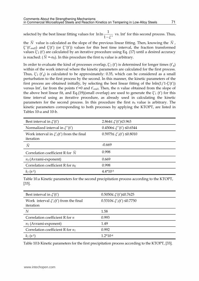
kinetic parameters corresponding to both processes by applying the KTOPT, are listed in Tables 10-a and 10-b.
Best interval in ’(t’) 2.864≤ ’(t’)≤3.963
Normalized interval in ’’(t’) 0.4506≤ ’’(t’) ≤0.6544
Work interval in ’2(t’) from the final iteration
0.5975≤ ’2(t’) ≤0.8010
N -0.669
Correlation coefficient R for N 0.998
n2 (Avrami-exponent) 0.669
Correlation coefficient R for n2 0.998
k2 (s-1) 4.4*10-5
Table 10.a Kinetic parameters for the second precipitation process according to the KTOPT, [33].
Best interval in ’(t’) 0.5050≤ ’(t’)≤0.7625
Work interval ’1(t’) from the final iteration
0.5310≤ ’1(t’) ≤0.7750
N 1.58
Correlation coefficient R for n 0.993
n1 (Avrami-exponent) 1.49
Correlation coefficient R for n1 0.992
k1 (s-1) 1.2*10-4
Table 10.b Kinetic parameters for the first precipitation process according to the KTOPT, [33].
www.intechopen.com

Alloy Steel – Properties and Use
72
3.1.4 Uncertainty in the Avrami-exponent
In order to estimate the error-prone Avrami-exponent (n’), the uncertainty in the fraction transformed ’(t’) for both work interval is determined according to the procedure described in [44], where:
n’=nn with n=[1 ln(1 ')]
'(1 ')ln(1 ')n
(22)
Let us define the parameters: y’=Δl’(t’)/L0=(l’(t’)-L0)/L0, y’1= Δl’(t’end1)/L0, and y’0= Δl’(0)/L0. The uncertainty ’(t’) is obtained by the propagation of the uncertainty corresponding to the length changes measured directly from the dilatometry curve (l’=10-3mm). Then:
1 0 02
0 1 0
2[( ' ' ) ( ' ' )]'( ') '
( ' ' )
y y y yt l
L y y (23)
For the best work interval corresponding to the second process, the selected parameters for calculating the error-prone Avrami-exponent (n’2) are: y’=5.815*10-4, y’1=2.2*10-4 and y’0=0.98*10-4; then ’=0.8. As ┙l>0, the uncertainty n2 for the boundary values of the fraction transformed ’2(t’) in the above selected work interval is: n2=-0.02 for ’2=0.5976 and n2=0.18 for ’2=0.801 [33]. In this manner, the Avrami-exponent n2 with its error bounds can be written as: 0.65<0.67<0.69 or n’2=0.670.02.
In order to calculate the Avrami-exponent corresponding to the first process, a similar procedure to the second one is applied. The same parameters y’1 and y’2 are selected, but the y’ parameter is now 1.91*10-4 as the extreme value of the fraction transformed ’(t’) for the best time interval corresponding to the first process from the dilatometry curve.
The uncertainty ’(t’) according to Eq. (23) for the first process is ’(t’)0.28 and assuming a small overlap situation, ’1=(n1/n)’0.2. The uncertainty in the Avrami exponent n1 resulted to be: n1=-0.2 for ’1(t’)=0.531 and n1=0.4 for ’1(t’)=0.775. The Avrami-exponent for this first process, n1 with its smallest error bounds, can be written as: 1.29<1.49<1.69 or n’1=1.50.2.
3.1.5 Precipitation processes on tempering
The results obtained by the proposed approach (n1=1.5) show that the first process identified in the dilatometry curve (by an initial contraction of length) corresponds to a diffusion-controlled precipitation process during which small particles grow with zero nucleation rate (n1=1.5) [31, 45]. This first stage of tempering is recognized in the literature as the decomposition of martensite into transition carbide (┝ or ┟-carbides) and a less tetragonal martensite [46]. The precipitation of the transition carbide could have occurred in very early stages of tempering or during quenching for this alloy; the Ms temperature is about 365°C [47]. This transition carbide is frequently observed to nucleate uniformly throughout the martensite matrix and some studies [48, 49] have indicated that the nucleation may be influenced by the modulated structure formed by spinodal decomposition that occurs before the first stage. It is also reported in other works [50], that the initial formation of the first transition carbide is due to a shear of the martensite structure which would involve neither
www.intechopen.com

Comments About the Strengthening Mechanisms in Commercial Microalloyed Steels and Reaction Kinetics on Tempering in Low-Alloy Steels
73
carbon diffusion nor a significant initial fall in hardness. According to the literature [46, 48, 51], there is no evidence that the nucleation of the transition carbide (┝ or ┟ carbide) could be related to the dislocations in the martensite.
The second process identified in the dilatometry curve by a second contraction in length, corresponds to the disappearance of the transition carbide and the formation of stable cementite. Many articles [52, 53] report that cementite nucleates on dislocations, inter-lath and grain boundaries. In this sense, an Avrami-exponent n2=0.67 is in agreement with a mechanism that involved precipitation on dislocations and diffusion-controlled growth (n=0.66) [45].
3.2 Non-isothermal tempering
3.2.1 Introduction
In the past, a number of methods have been proposed to describe the progress of a reaction in solid systems from non-isothermal experiments. Although non-isothermal experiments can use any arbitrary thermal history, the most usual in thermal analysis is to employ a constant heating rate, (┚ = dT/dt =const).
In order to study the kinetics of the phase transformations performed at constant heating rates (┚), a wide range of methods has been established for deriving the kinetic parameters of the reactions obeying equations:
( ) ( )d
K T gdt
(24)
and
0( ) exp[ ]E
K T KRT
(25)
where g() is a specific function of the fraction transformed, K(T) is the rate constant of the reaction mechanism and E, K0 and R are the activation energy of the reaction mechanism, the frequency factor and the gas constant respectively [54]. Thus, without recourse to any kinetic model, values for effective activation energy can be obtained upon isochronal experiments from the temperatures T needed to attain a certain fixed value of (temperatures corresponding to the same degree of transformation), as measured for different heating rates (┚)[55]. The procedures that use the above temperatures T for calculating the effective activation energy are known as Kissinger-like methods [54, 55], and these rely on approximating the so-called temperature integral [55-58]. Another set of methods does not use any mathematical approximation for calculating the temperature integral, but instead require determinations of the reaction rates at a stage with the same degree of transformation (it corresponds to an equivalent stage of the reaction) for various heating rates. These procedures are known as the Friedman-like methods [59].
As the determination of g(), E and K0 (the so-called kinetic triplet) is an interlinked problem in non-isothermal experiments[54,60], a deviation in the determination of any of the three will cause a deviation in the other parameters of the triplet. Thus, it is important to start the
www.intechopen.com
Alloy Steel – Properties and Use
74
analysis of a non-isothermal experiment by determining one element of the triplet with high accuracy. In this sense, it is usual to calculate the effective activation energy (E) by a Kissinger-like method for nucleation and growth reactions [55, 61, 62]. This is because the T constitutes a parameter that can be determined with high accuracy in some non-isothermal experiments, such as in non-isothermal dilatometry curves. For nucleation and growth reactions, in general, the effective activation energy is a function of both transformation time and temperature (E does not have to be constant even with constant nucleation and growth mechanisms). Because of this, the above lineal approximation of the Kissinger-like plot will be strictly valid only if the effective activation energy is constant during the entire transformation [62]. This condition is initially ignored in most papers. Thus, this research has been devised to explore the possibilities that combination of the different non-isothermal analysis methods has to obtain the kinetic parameters of the tempering reactions in low-alloy steels using non-isothermal dilatometric data [63].
3.2.2 Non-isothermal dilatometric analysis: Theoretical background and experimental procedure
The precipitation reactions in isothermal conditions are generally described by the JMAK-like relation [64-66]:
1 exp ( )n with ( )K T t (26)
where n is known as the Avrami exponent and t is the time.
In order to maintain the JMAK description under non-isothermal conditions, the formalism of Eq. (26) is accepted for an infinitesimal lapse of time [61, 67]:
0 exp( )E
d K dtRT
(27)
Integration of Eq.(27), resulted in:
2
02
( ) [ exp( )][1 ]T R E RT
T KE RT E
(28)
After deriving 0
1 0
( )p p
pp p
twice with respect to T, evaluating the resulted equation at
temperatures corresponding to the inflection points Ti [55], and taking into account several mathematical approximations, it is obtained the working expression [61, 67]:
2 Re 1 Re 2*
o
ii
RKELn Ln s s
R T ET
(29)
with:
2
2Re 1 iQRTs
n E and
2
2
( )1Re 2 2 * 1 ln i i iT RK T RT
s nE En
(30)
www.intechopen.com

Comments About the Strengthening Mechanisms in Commercial Microalloyed Steels and Reaction Kinetics on Tempering in Low-Alloy Steels
75
here
1 0
1 0
( ) 2p
dp dp
dT dTQ Tp p
Ti (31)
If both residuals are neglected in Eq. (29) (see appendix in [63]), the data points in a plot of the ln┚/Ti2 versus 1/Ti (Kissiger-like plot) are approximated by a straight line, from the slope of which a value for the effective activation energy, E, is obtained. We settle that with the definition of the state variable ┠ (c.f. ref. 55 and 62), the adoption of a specific model of reaction is not a necessary condition to obtain the effective activation energy from the slope of a Kissinger-like plot.
An analytical solution of the JMAK rate equation for the general non-isothermal case at constant heating rate, assuming that the nucleation (N) and growth (G) rates have an Arrhenian dependence of temperature has been published [68]:
01n
E EExp K C P
R RT
(32)
where it is considered that the transformation rate is negligible at the initial temperature of the experiment.
In this expression, P(E/RT) is the exponential integral, and C a constant that depends on n, EN and EG(activation energies for nucleation and growth mechanisms). The constant C reduces to unity in particular situations when the nucleation is completed prior to crystal growth (site saturation situation) or in the isokinetic situation where EN=EG [68].
In order to obtain a suitable Kissinger-like plot (ln[┚/Tp2] versus 1/Tp), the authors [68], without recourse to any kinetic model, obtained the relation:
02
'( )ln ln[ ]p
pp
RK CgE
RT ET
(33)
As a JMAK kinetic model is assumed, then:
1
( ) (1 )[ ln(1 )]n
ng n and 1
( ) 1'( )
1[ ln(1 )]n
dg g ng
d
(34)
It has been demonstrated that in the peak temperature, P=0.632 and therefore g’(Tp)=-1, [68]. Eq.(33) can be now applied to the non-isothermal dilatometry data at temperatures Ti, corresponding to the inflection points for different constant heating rates (the temperatures Ti belong with very good approximation to an equivalent stage of the reaction [55], Ti=0.632).
Then, as it can be seen, Eq.(33) coincides with Eq.(29) in the isokinetic case (EN=EG) , or in the site saturation situation (C=1), if both residuals in Eq.(29) are neglected.
www.intechopen.com

Alloy Steel – Properties and Use
76
In order to calculate the parameters K0 and C a non linear regression analysis is performed using Eq. (33) where Tp has been changed by Ti and g’(Ti)=-1 at the inflection points. Consequently, it is possible to obtain a transcendent equation to find n through the second derivative of Eq.(32):
10 2
( )( ) [ ] [ ( )] exp( ) ( 1) exp( ) 0n n n i
i i i i
EEp
RTE E E R En K C p n
R RT RT E RT RT
(35)
An alternative method to estimate the effective activation energy and other kinetic parameters directly from the non-isothermal dilatometry curves is presented in [69]. Furthermore, this procedure allows analyzing if the effective activation energy, obtained by the above Kissinger-like plot, is constant during the entire transformation. For this, the
fraction untransformed (1-), according to 0
1 0
( )p p
pp p
with p=Δl/l (relative change of
length), is defined as:
0( ) ( ) l(T) ( )
(1 ) [( ) ( ) ]/[( ) ( ) ]lT end end
l T l T l T
l l l (36)
where (Δl(T) /l)0 and (Δl(T) /l)end are the relative length increments of the start and end stages, at temperature T. The (Δl(T) /l)T is the relative length increment on dilatometric curve at temperature T, as it is depicted in Figure 6. According to this definition (1-)=1 and =0 at the start temperature of the transformation T=Ts.
This procedure was applied to nucleation and growth reactions (tempering reactions in
steels) using an expression oversimplified for g()= 0n(1- ) [69]. This way, the analysis is
based on the assumption of homogeneous reactions with a reaction rate:
Fig. 6. Relative length change (Δl(T) / l ) near the inflection point [63]
www.intechopen.com

Comments About the Strengthening Mechanisms in Commercial Microalloyed Steels and Reaction Kinetics on Tempering in Low-Alloy Steels
77
0n(1 )(1- )
dK
dt
(37)
where the order of the tempering reaction under consideration is n0.
Differentiation of Eq.(37) (with ┚ as a constant and exp( / )oK K E RT ), and its evaluation
at the inflection point temperature (Ti) on the curve (1-) versus temperature, the equation for the effective activation energy is obtained:
0
0
12 (1 )(1 )
(1 )
no i Ti
Tin
Ti
dn RT
dTE
(38)
The other kinetic parameters can be calculated through the equations:
0
0(1 )
exp( )(1 ) n
iTi Ti
d EK
dT RT
(39)
and:
0
0
(1 )(1 ) [ ] exp( )n
TT
d E
K dT RT
(40)
Although the above simplification could be questioned, this approximation may be used to investigate the variation of the effective activation energy under different experimental conditions [70]. In order to solve this difficulty it is assumed that the tempering reactions obey a JMAK kinetic model. Therefore, if the above formalism for homogeneous transformations is settled; then, a relationship between the Avrami exponent n and the kinetic order of the reaction n0 can be obtained as a function of the fraction untransformed (1-). Thus, the transformation rate for a reaction that obeys a JMAK relation is:
1
(1 ) (1 ) ( ln(1 ))n
nd
K ndt
(41)
From the Eqs. (37) and (41), the expression that related n, n0 and (1-) resulted to be:
1
0ln[ ( ln(1 )) ]
1ln(1 )
n
nnn
(42)
As it is shown in Figure 7, the behavior of the n0 function depends weakly on (1-) far from the boundary point (1-)=1. As a consequence, n0 can be considered as a constant during the development of the reaction for stages where the fraction transformed is greater than 0.4. Also, the n0 values are lower the greater the Avrami exponent, and when the Avrami exponent takes the value n=1, the reaction is the first order (n0=1). Evaluation of n0 from the different nucleation and growth protocols, given by the n values, makes possible to use the procedure established in [69] to nucleation and growth reactions and therefore to determine
www.intechopen.com

Alloy Steel – Properties and Use
78
if E is constant during the entire transformation. For this, the fraction untransformed values calculated from Eq. (40) (where it is used the E value determined by a Kissinger-like plot) for the entire reaction are compared with the experimental fraction untransformed data obtained from the dilatometric curve.
Fig. 7. Behavior of the n0 parameter versus the fraction untransformed (1-) for different Avrami exponent values [63]
The Friedman-like methods conceived to be used in processing of non-isothermal calorimetric data do not require any mathematical approximation to solve the temperature or exponential integral [54, 59]. This procedure allows obtaining the activation energy of a reaction knowing the reaction rates at a stage with the same degree of transformation for various heating rates. According to the knowledge of the present authors [63], the Friedman-like methods have not been very much used with non-isothermal dilatometry data.
In fact, if d/dt at temperatures corresponding to the inflection points (Ti) is known then, substituting the K(T) expression into dξ/dt equation ( ┚= dT/dt); the following equation results after applying logarithms to both terms:
0ln[ ] ln[ ] ln( ( ))i iT T i
i
d d EK g
dt dT RT
(43)
As in the dilatometry record one has that ( ) tt
l ll
l l
, where l is the initial length of the
sample and lt is the length at any instant, then:
t
t
ldl dl
dT dT l
(44)
Differentiating 0
1 0
( )p p
pp p
with respect to time (with p=l
l
), and taking into account Eq.
(44); Eq. (43) can be written, at temperatures corresponding to the inflection points, as [63]:
www.intechopen.com
Comments About the Strengthening Mechanisms in Commercial Microalloyed Steels and Reaction Kinetics on Tempering in Low-Alloy Steels
79
lniTi
d l EConst
dT l RT
(45)
According to Eq.(45) it is possible to calculate the effective activation energy E, (but not the frequency factor, K0 ).
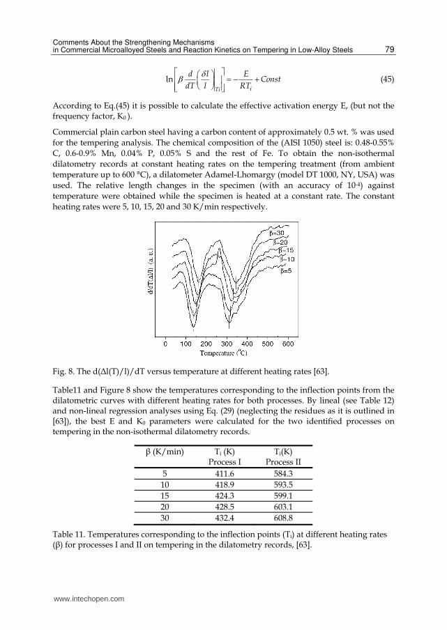
Commercial plain carbon steel having a carbon content of approximately 0.5 wt. % was used for the tempering analysis. The chemical composition of the (AISI 1050) steel is: 0.48-0.55% C, 0.6-0.9% Mn, 0.04% P, 0.05% S and the rest of Fe. To obtain the non-isothermal dilatometry records at constant heating rates on the tempering treatment (from ambient temperature up to 600 °C), a dilatometer Adamel-Lhomargy (model DT 1000, NY, USA) was used. The relative length changes in the specimen (with an accuracy of 10-4) against temperature were obtained while the specimen is heated at a constant rate. The constant heating rates were 5, 10, 15, 20 and 30 K/min respectively.
Fig. 8. The d(Δl(T)/l)/dT versus temperature at different heating rates [63].
Table11 and Figure 8 show the temperatures corresponding to the inflection points from the dilatometric curves with different heating rates for both processes. By lineal (see Table 12) and non-lineal regression analyses using Eq. (29) (neglecting the residues as it is outlined in [63]), the best E and K0 parameters were calculated for the two identified processes on tempering in the non-isothermal dilatometry records.
┚ (K/min) Ti (K) Process I
Ti(K) Process II
5 411.6 584.3 10 418.9 593.5 15 424.3 599.1 20 428.5 603.1 30 432.4 608.8
Table 11. Temperatures corresponding to the inflection points (Ti) at different heating rates (┚) for processes I and II on tempering in the dilatometry records, [63].
www.intechopen.com

Alloy Steel – Properties and Use
80
Process ActivationEnergy, E
KJ/mol
FrequencyFactor, K0
min-1
Confidence Interval for E Regression Coefficient
R
P value for E
I 117 2.99*1014 104< E<130 (*) 116.5<E<117.4 (**)
0.998 (**) 4.8 *10-10 (**)
II 206 9.53*1017 196<E<216 (*)
205.6<E<206.4 (**)
0.999(**) 9.0*10-14 (**)
(*) Lineal regression analysis (**) Non-lineal regression analysis (E and K0 are the fitting parameters) P=Distr. T(T, FD, 2): It represents the probability that a better fit to the same data can be carried out by another model. As the P values are very low, it is not very probable that another model fits the data better than the model here shown.
Table 12. Best parameters E and K0 calculated by linear and non-lineal regression analyses respectively for the two processes on tempering using Eq.(29) where both residuals have been ignored, [63].
Although one has the possibility, with this procedure (Eqs. (29-31)), to obtain a relationship for calculating the Avrami exponent (n) of the reaction, we think that the n values are not very reliable due to the many approximations used to obtain the residues. For this reason, the use of the transcendent equation, Eq.(35), is very much reliable to calculate n, given by much less approximations in their determination. In this sense, as a first step, the K0 and C parameters are calculated according to a procedure detailed in [63]. Table 13 shows the Avrami exponent for each considered process on tempering at different heating rates solving the transcendent equation, Eq. (35).
┚ (K/min) Ti (K) n ├n
5 411.6 1.2 0.2
10 418.9 1.1 0.2
15 424.3 1.0 0.2
20 428.5 1.1 0.2
30 432.4 1.0 0.2
First Process on Tempering
β (K/min) Ti (K) n δn
5 584.3 0.7 0.1
10 593.5 0.7 0.1
15 599.1 0.7 0.1
20 603.1 0.7 0.1
30 608.8 0.7 0.1
Second Process on Tempering
Table 13. The Avrami exponent for the two processes on tempering, [63]
www.intechopen.com

Comments About the Strengthening Mechanisms in Commercial Microalloyed Steels and Reaction Kinetics on Tempering in Low-Alloy Steels
81
The uncertainty showed in each Avrami exponent value (├n) (Table 13) was calculated by the propagation of the uncertainty [44] in temperature (├T=0.1°C) and in the activation energy (E=0.5 KJ/mol calculated by non-linear regression analysis of Eq.(33)) from the transcendent equation F(n, T, E)=0, [63].
After this, it is concluded that the first process on tempering considered by us corresponds to a reaction with n0=1 according to the formalism showed in [69]. On the contrary, the second process (third stage of tempering) that in the literature is identified as the cementite precipitation, the n0 parameter has a value close to 1.4 (n=0.66) according to Eq.(42).
Taking the above n0 values for the first and second processes respectively, the new E values at temperatures of the inflection points can be determined by Eq.(38). As can be seen in Tables 14 and 15, these values are the same, within the error boundary, as those obtained by a Kissinger-like plot. The frequency factors for each heating rate are calculated by the use of Eq.(39).
β Ti(K) n0 K0 (min-1) E(KJ/mol) δE(KJ/mol)
5 411.6 1.0 5.4 *1014 119 6
10 418.9 1.0 6.87 *1013 112 6
15 424.3 1.0 3.3 *1014 117 6
20 428.5 1.0 2.0 *1015 124 7
30 432.4 1.0 1.1*1014 113 6
Table 14. Activation energies (E) and the frequency factors (K0) for the first process on tempering using Eq.(38) and (39), [63].
β Ti(K) n0 K0*1017(min-1) E(KJ/mol) δE(KJ/mol)
5 584.3 1.4 1.3 196 11
10 593.5 1.4 1.2 196 10
15 599.1 1.4 1.3 196 10
20 603.1 1.4 1.6 197 10
30 608.8 1.4 1.3 196 10
Table 15. Activation energies (E) and the frequency factors (K0) for the second process on tempering using Eq.(38) and (39), [63].
According to Eq. (40), the fraction untransformed values are calculated for the entire range of temperatures using the determined E, K0 and n0 values. Only for the above n0 values, the calculated effective activation energy is constant for the entire reaction, Figure 9. Other nucleation and growth protocols, that generate another n0 values, cause appreciable deviations among the experimental and calculated fraction untransformed values for the range of temperatures where the reactions are developed.
www.intechopen.com

Alloy Steel – Properties and Use
82
Fig. 9. Fraction untransformed versus temperature according to Eq. (40): Experimental curves for the first (I) and second (II) processes with a heating rate: ┚=5 0C/min. The symbols: filled triangle and filled circle are the fraction untransformed values calculated by Eq.(40) for different temperatures. Process (I): K0=5.4x10¹⁴ min-1; E=119 KJ/mol; no=1; d(1-) ⁄dT│Ti =-0.032275. Process (II): K0=1.3 x10¹⁷ min-1; E=196 KJ/mol; no=1.4; d(1-) ⁄dT│Ti =-0.0184273 [63].
The d/dT(├l/l) data used in the determination of the effective activation energy by a Friedman-like procedure is shown in [63]. By linear fitting of Eq.(45), the effective activation energy was for both processes: E=127.5 KJ/mol; ├E=32.7 KJ/mol (first process) and E=202.9 KJ/mol; ├E=40 KJ/mol (second process), very close to those determined by a Kissinger-like method.
3.2.3 Precipitation processes on tempering
Considering the chemical composition of steel and the results obtained by the analysis of the dilatometry records, it is assumed that the new nuclei corresponding to the first stage of tempering could have been formed during the quench. This is because in the studied steel, the Ms temperature (martensite start temperature) is closed to 300°C according to the Ms relation for 0.5 wt % C and 0.8 wt % Mn[71], and by the greater mobility of the carbon atoms through the dislocations inherited from the martensite structure[72].
In the temperature range of approximately 100°-200° C (see Figure 8) for the first processes at the non-isothermal dilatometric registers, the transition carbide (epsilon carbide) nuclei that have been formed on quenching are growing. The growth of the transition carbide produces a lost of tetragonality of the martensite matrix by the exit of the interstitial carbon in solution. The above is in agreement with the situation where existing nuclei in form of needles or plates are developed by controlled diffusion growth corresponding to the Avrami exponent close to one (n=1)[45] as it is shown in Table 13 for this first process on tempering.
www.intechopen.com
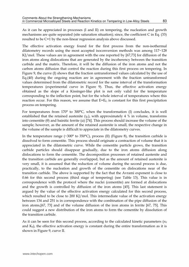
Comments About the Strengthening Mechanisms in Commercial Microalloyed Steels and Reaction Kinetics on Tempering in Low-Alloy Steels
83
As it can be appreciated in processes (I and II) on tempering, the nucleation and growth mechanisms are quite separated (site saturation situation); since, the coefficient C in Eq. (33) resulted to be C=1 by the non-linear regression analysis above discussed.
The effective activation energy found for the first process from the non-isothermal dilatometry records using the most accepted isoconversion methods was among 117~128 KJ/mol. These values are in agreement with the one reported by [67,73] for diffusion of the iron atoms along dislocations that are generated by the incoherency between the transition carbide and the matrix. Therefore, it will be the diffusion of the iron atoms and not the carbon atoms diffusion that control the reaction during this first process on tempering. In Figure 9, the curve (I) shows that the fraction untransformed values calculated by the use of Eq.(40) during the ongoing reaction are in agreement with the fraction untransformed values determined from the dilatometric record for the same interval of the transformation temperatures (experimental curve in Figure 9). Thus, the effective activation energy obtained as the slope of a Kissinger-like plot is not only valid for the temperature corresponding to the inflection point, but for the whole interval of temperatures where this reaction occur. For this reason, we assume that E=EG is constant for this first precipitation process on tempering.
For temperatures from 170° to 300°C, when the transformation (I) concludes, it is well established that the retained austenite (┛r), with approximately 4 % in volume, transforms into cementite (┠) and bainitic ferrite (┙) [74]. This process should increase the volume of the sample; however, as the amount of the retained austenite is small, the respective change in the volume of the sample is difficult to appreciate in the dilatometry curves.
In the temperature range (~300° to 350°C), process (II) (Figure 8), the transition carbide is dissolved to form cementite. This process should originate a contraction of volume that it is appreciated in the dilatometric curve. While the cementite particle grows, the transition carbide particles should disappear gradually, due to the iron atoms diffusion along dislocations to form the cementite. The decomposition processes of retained austenite and the transition carbide are generally overlapped, but as the amount of retained austenite is very small, it is assumed that the reduction of volume during the second process is due, practically, to the nucleation and growth of the cementite on dislocations near of the transition carbide. The above is supported by the fact that the Avrami exponent is close to 0.66 for this second process (third stage of tempering) (see Table 13). This value is in correspondence with the protocol where the nuclei (cementite) are formed at dislocations and the growth is controlled by diffusion of the iron atoms [45]. This last statement is argued by the value of the effective activation energy calculated for this second process, which resulted to be close to 200 KJ/mol. This intermediate value of the activation energy between 134 and 251 is in correspondence with the combination of the pipe diffusion of the iron atoms,[67, 73] and of the volume diffusion of the iron atoms in ferrite [67, 75]. This could suggest a new distribution of the iron atoms to form the cementite by dissolution of the transition carbide.
As it can be seen for this second process, according to the calculated kinetic parameters (n0 and K0), the effective activation energy is constant during the entire transformation as it is shown in Figure 9, curve II.
www.intechopen.com

Alloy Steel – Properties and Use
84
4. References
[1] T. Gladman, The Physical Metallurgy of Microalloyed Steels, The Institute of Materials, London (1997), p 28-57.
[2] H.-J. Kestenbach and E. V. Morales, Transmission Electron Microscopy of Carbonitride Precipitation in Microalloyed Steels, Acta Microscópica, (1998), 7(1): 22-33.
[3] W. B. Morrison and J.H. Woodhead, The influence of small niobium additions on the mechanical properties of commercial mild steels. J. Iron Steel Inst. (1963), 201:43-46.
[4] W. B. Morrison, The influence of small niobium additions on the properties of carbon-manganese steels. J. Iron steel Inst. (1963), 201:317-325.
[5] J. M. Gray, D. Webster, and J. H. Woodhead, J. Iron Steel Inst. (1965), 203:812-818. [6] H.-D. Bartholot, H.-J. Engell, W. Vordemesche, and K. Kaup, Stahl Eisen, (1971), 91:204-
219. [7] T. Gladman, D. Dulieu, and I. D. McIvor, Microalloying 75, Union Carbide Corporation,
New York, (1977), p 32-55. [8] T. Gladman, B. Holmes, and I. D. McIvor, The effects of second phase particles on the
mechanical properties of steel, The Iron and Steel Institute, London, (1971) p 68-78. [9] A. Itman, K. R. Cardoso, and H.-J. Kestenbach, Mater. Sci. Technol. (1997), 13:49-55. [10] A. T. Davenport, L. C. Brossard, and R. E. Miner, J. Met., (1975), 27:21-27. [11] F. B. Pickering, Microalloying 75, Union Carbide Corporation, New York, (1977), p 9-
30. [12] A. J. DeArdo, 8th process technology conference, The Iron and Steel Society,
Warrendale, PA, (1988) p 67-78. [13] L Meyer, C. Strassburger, and C. Schneider, HSLA steels: metallurgy and applications,
American Society for Metals, Metals Park, OH, (1986) p 29-44. [14] E. Valencia Morales, and H.-J. Kestenbach, Rev. Metal. Madrid, (1998), 34(6):488-498. [15] S. S. Campos, E. V. Morales, and H.-J. Kestenbach, Metall. Mater. Trans. (2001),
32A:1245-1248. [16] S. S. Campos, J. Gallego, E. V. Morales, and H.-J. Kestenbach, HSLA Steels 2000, (ed.
Liu Guoquan et al.), Metallurgical Industry Press, Beijing, (2000) p 629-634. [17] S. Freeman, and R. W. K. Honeycombe, Met. Sci., (1977), 11:59-64. [18] R. M. Brito, and H.-J. Kestenbach, J. Mater. Sci., (1981), 16:1257-1263. [19] F. B. Pickering and T. Gladman, Metallurgical Developments in Carbon Steels, Iron
and Steel Institute, Special Report Nº 81, (1963), p 10. [20] M. F. Ashby, Strength Methods in Crystals, A. Kelly and R. B. Nicholson, eds. Elsevier,
London, (1971) p 137. [21] A. S. Keh and S. Weissmann, Electron Microscopy and Strength of Crystals, G. Thomas
and J. Washburn, eds., Interscience Publishers, New York, NY, (1963), p 231. [22] J. M. Rosenberg and H. R. Piehler, Metall. Trans., (1971), 2: 257-259. [23] F. R. N. Nabarro, Z. S. Basinski, and D. B. Holt, Adv. Phys., (1964), 13: 193-198. [24] R. W. K. Honeycombe, HSLA Steels: Metallurgy and Applications, Beijin Conf., ASM,
Metals Park, OH, (1986), p 243-250. [25] A. S. Keh, Direct Observations of Imperfections in Crystals, J. B. Newkirk and J.
H.Wernick, eds., J. Wiley, London, (1962), p. 213. [26] H.-J. Kestenbach, S. S. Campos, and E. V. Morales, Mater. Sci. Technol. (2006),
22(6):615-626. [27] A. D. Batte, and R. W. K. Honeycombe, J. Iron Steel Inst., (1973), 211:284-289.
www.intechopen.com

Comments About the Strengthening Mechanisms in Commercial Microalloyed Steels and Reaction Kinetics on Tempering in Low-Alloy Steels
85
[28] J.D. Robson, Modelling of carbide and laves phase precipitation in 9-12wt% chromium Steels, Ph.D. diss, University of Cambridge, UK, 1996.
[29] P. Wilkes, Met. Sci. J., (1968), 2:8-17. [30] J.K.L. Lai and M. Meshkat, Metal Science, (1978), 9:415-420. [31] M.J. Starink, J. Mater. Sci., (1997), 32:4061-4070. [32] Eon-Sik Lee and Y.G. Kim, Acta Metall. Mater., (1990), 38:1669-1676. [33] E. V. Morales, J. A. Vega-Leiva, H.L. Lopez Salinas, and I. S. Bott, Phase Transitions,
(2011), 84(2):179 -191. [34] K. Hanawaka and T. Mimura, Metall Trans A, (1984), 15:1147-1153. [35] N.J. Luiggi and A. Betancourt, Metall. Trans. B, (1994), 25:917-925. [36] N.J. Luiggi and A. Betancourt, Metall. Trans. B, (1994), 25:927-935. [37] N.J. Luiggi and A. Betancourt, Metall Trans B, (1997), 28:161-168. [38] A.T.W. Kempen, F. Sommer and E.J. Mittemeijer, J. Mater. Sci., (2002), 37:1321-1332. [39] F. Liu, F. Sommer and E.J. Mittemeijer, J. Mater. Sci., (2004), 39:1621-1634. [40] D. Wang, Y. Liu, Z. Gao and Y. Zhang, J. Non-Cryst. Solids, (2008), 354:3990-3999. [41] D. Wang, Y. Liu and Y. Zhang, J. Mater. Sci., (2008), 43:4876-4885. [42] D. Wang, Y. Liu, C. Bao, W. Tan and Z. Gao, Appl. Phys. A, (2009), 96:721-729. [43] E.V. Morales, N.J. Galeano, J.V. Leiva, L.M. Castellanos, C.E. Villar and R.J.
Hernández, Acta Mater., (2004), 52:1083-1088. [44] E.V. Morales, J.V. Leiva, C.E. Villar, M.J. Antiquera and R.C. Fadragas, Scripta Mater.,
(2005), 52:217-219. [45] J.W. Christian, The theory of transformations in metals and alloys, Part I. 2nd ed.
Oxford: Pergamon Press, 1975, p 525-548. [46] Y. Wang, S. Denis, B. Appolaire and P. Archambault, J. Phys. IV, France, (2004), 120:103-
110. [47] E.R. Parker, Metall. Trans. A, (1977), 8A:1025-1042. [48] K.A. Taylor, G.B. Olson, M. Cohen and J.B. Vander Sande, Metall. Trans. A, (1989),
20A:2749-2765. [49] S. Nagakura, Y. Hirotsu, M. Kusunoki, T. Suzuki and Y. Nakamura, Metall. Trans. A,
(1983), 14A:1025-1031. [50] M. Dirand and L. Afqir, Acta Metall., (1983), 31:1089-1107. [51] E. Tekin and P.M. Kelly, Precipitation from iron-base alloys. G.R. Speich and J.B. Clark
Eds. Metall. Soc. Conference. Cleveland, vol. 28, 1963, p 173-229. [52] Y. Imai, T. Ogura and A. Inoue, Trans ISIJ., (1973), 13:183-191. [53] J. Nutting, J.I.S.I., (1969), 207:872-893. [54] M. J. Starink, Thermochim. Acta. (2003), 404:163-176. [55] E.J. Mittemijer, J. Mater. Sci., (1992), 27:3977-3987. [56] H.E. Kissinger, J. Res. Nat. Bur. Stand., (1956), 57:217-221. [57] H.E. Kissinger, Anal. Chem. (1957), 29:1702-1706. [58] Órfáo J.J.M. AIChE Journal, (2007), 53:2905-2915. [59] H.L. Friedman, J. Polym. Sci. (1964), C6:183-195. [60] J.D. Sewry and M.E. Brown, Termochim. Acta, (2002), 390:217-245. [61] E.J. Mittemeijer, A. Van Gent and P.J. Van der Schaaf, Metall. Trans. A, (1986),
17A:1441-1445. [62] F. Liu, F. Sommer, C. Bos and E. J. Mittemeijer, International Mater. Reviews, (2007),
52:193-212.
www.intechopen.com

Alloy Steel – Properties and Use
86
[63] J. A. V. Leiva, E. V. Morales, E. Villar-Cociña, C. A. Donis and Ivani de S. Bott, J. Mater. Sci., (2010), 45:418–428.
[64] A.N. Kolmogorov, Izv. Akad. Nauk. USSR-Ser. Matemat., (1937), 1:355-360. [65] W.A. Johnson and R. F. Mehl, Trans. AIME. (1939), 135:416-460. [66] M. Avrami, J. Chem. Phys. (1939), 7:1103-1112. [67] L. Cheng, C.M. Brakman, B.M. Korevaar and E. J. Mittemeijer, Metall. Trans. A, (1988),
19A:2415-2426. [68] J. Farjas and P. Roura, Acta Mater., (2006), 54:5573-5579. [69] Y. Tomita, J. Mater. Sci., (1989), 24:731-735. [70] J. Sestak, A. Brown, V. Rihak and G.Berggren, (1969), in Thermal Analysis. Academic
Press. N.Y. p 1035. [71] W. Stevens and A.G. Haynes, J. Iron Steel Inst., (1956), 183:349-357. [72] Y. Hirotsu and S. Nagakura, Acta Metall., (1972), 20:645-655. [73] M. Cohen, Trans. J.I.M., (1970), II:145-151. [74] R.W.K. Honeycombe, (1981), Steels Microstructure and Properties, Edward Arnold Editions,
Chapter 8, p 142. [75] F. S. Buffington, K. Hirano and M. Cohen, Acta Metall., (1961), 9:534-539.
www.intechopen.com

Alloy Steel - Properties and UseEdited by Dr. Eduardo Valencia Morales
ISBN 978-953-307-484-9Hard cover, 270 pagesPublisher InTechPublished online 22, December, 2011Published in print edition December, 2011
InTech EuropeUniversity Campus STeP Ri Slavka Krautzeka 83/A 51000 Rijeka, Croatia Phone: +385 (51) 770 447 Fax: +385 (51) 686 166www.intechopen.com
InTech ChinaUnit 405, Office Block, Hotel Equatorial Shanghai No.65, Yan An Road (West), Shanghai, 200040, China
Phone: +86-21-62489820 Fax: +86-21-62489821
The sections in this book are devoted to new approaches and usages of stainless steels, the influence of theenvironments on the behavior of certain classes of steels, new structural concepts to understand some fatigueprocesses, new insight on strengthening mechanisms, and toughness in microalloyed steels. The kineticsduring tempering in low-alloy steels is also discussed through a new set-up that uses a modified Avramiformalism.
How to referenceIn order to correctly reference this scholarly work, feel free to copy and paste the following:
Eduardo Valencia Morales (2011). Comments About the Strengthening Mechanisms in CommercialMicroalloyed Steels and Reaction Kinetics on Tempering in Low-Alloy Steels, Alloy Steel - Properties and Use,Dr. Eduardo Valencia Morales (Ed.), ISBN: 978-953-307-484-9, InTech, Available from:http://www.intechopen.com/books/alloy-steel-properties-and-use/comments-about-the-strengthening-mechanisms-in-commercial-microalloyed-steels-and-reaction-kinetics-

© 2011 The Author(s). Licensee IntechOpen. This is an open access articledistributed under the terms of the Creative Commons Attribution 3.0License, which permits unrestricted use, distribution, and reproduction inany medium, provided the original work is properly cited.
Related Documents