Commentary on the Makridakis Time Series Competition (M

University of Pennsylvania University of Pennsylvania

ScholarlyCommons ScholarlyCommons

Marketing Papers Wharton Faculty Research

1983

Commentary on the Makridakis Time Series Competition (M-Commentary on the Makridakis Time Series Competition (M-

Competition) Competition)

J. Scott Armstrong University of Pennsylvania, [email protected]

Edward J. Lusk

Follow this and additional works at: https://repository.upenn.edu/marketing_papers

Part of the Marketing Commons

Recommended Citation Recommended Citation Armstrong, J. S., & Lusk, E. J. (1983). Commentary on the Makridakis Time Series Competition (M-Competition). Journal of Forecasting, 2 259-311. Retrieved from https://repository.upenn.edu/marketing_papers/226

This paper is posted at ScholarlyCommons. https://repository.upenn.edu/marketing_papers/226 For more information, please contact [email protected].

https://repository.upenn.edu/

https://repository.upenn.edu/marketing_papers

https://repository.upenn.edu/wharton_faculty

https://repository.upenn.edu/marketing_papers?utm_source=repository.upenn.edu%2Fmarketing_papers%2F226&utm_medium=PDF&utm_campaign=PDFCoverPages

http://network.bepress.com/hgg/discipline/638?utm_source=repository.upenn.edu%2Fmarketing_papers%2F226&utm_medium=PDF&utm_campaign=PDFCoverPages

https://repository.upenn.edu/marketing_papers/226?utm_source=repository.upenn.edu%2Fmarketing_papers%2F226&utm_medium=PDF&utm_campaign=PDFCoverPages

https://repository.upenn.edu/marketing_papers/226?utm_source=repository.upenn.edu%2Fmarketing_papers%2F226&utm_medium=PDF&utm_campaign=PDFCoverPages

https://repository.upenn.edu/marketing_papers/226

mailto:[email protected]

Commentary on the Makridakis Time Series Competition (M-Competition) Commentary on the Makridakis Time Series Competition (M-Competition)

Abstract Abstract In 1982, the Journal of Forecasting published the results of a forecasting competition organized by Spyros Makridakis (Makridakis et al., 1982). In this, the ex ante forecast errors of 21 methods were compared for forecasts of a variety of economic time series, generally using 1001 time series. Only extrapolative methods were used, as no data were available on causal variables. The accuracies of methods were compared using a variety of accuracy measures for different types of data and for varying forecast horizons. The original paper did not contain much interpretation or discussion. Partly this was by design, to be unbiased in the presentation. A more important factor, however, was the difficulty in gaining consensus on interpretation and presentation among the diverse group of authors, many of whom have a vested interest in certain methods. In the belief that this study was of major importance, we decided to obtain a more complete discussion of the results. We do not believe that “the data speak for themselves.”

Keywords Keywords Forecasting, extrapolation models, economic time series, M-competition, makridakis

Disciplines Disciplines Business | Marketing

This journal article is available at ScholarlyCommons: https://repository.upenn.edu/marketing_papers/226

https://repository.upenn.edu/marketing_papers/226

1

Published in Journal of Forecasting, 2 (1983), 259-311.

Commentary on the Makridakis Time Series Competition (M-Competition)

Introduction to the Commentary The Accuracy of Alternative Extrapolation Models:

Analysis of a Forecasting Competition through Open Peer Review

J. Scott Armstrong and Edward J. Lusk Wharton School, University of Pennsylvania, U.S.A.

Abstract

In 1982, the Journal of Forecasting published the results of a forecasting competition organized

by Spyros Makridakis (Makridakis et al., 1982). In this, the ex ante forecast errors of 21 methods were compared for forecasts of a variety of economic time series, generally using 1001 time series. Only extrapolative methods were used, as no data were available on causal variables. The accuracies of methods were compared using a variety of accuracy measures for different types of data and for varying forecast horizons.

The original paper did not contain much interpretation or discussion. Partly this was by design, to

be unbiased in the presentation. A more important factor, however, was the difficulty in gaining consensus on interpretation and presentation among the diverse group of authors, many of whom have a vested interest in certain methods.

In the belief that this study was of major importance, we decided to obtain a more complete

discussion of the results. We do not believe that “the data speak for themselves.”

The Ground Rules

In seeking peer review of the Makridakis competition, we drew heavily upon the procedures used by Behavioral and Brain Sciences, a journal that has been one of the pioneers for open peer review (Harnad, 1979).

One objective was to provide a forum for discussion by experts who were likely to have different perspectives. We invited 14 outside experts to write commentaries on the Makridakis competition. Of these, eight agreed and seven completed their papers.

The commentators are all from different organizations. Three are practitioners and four are academicians.

We asked these commentators to address any aspect of the original paper. They were given approximately five months to write their commentary. We reviewed each commentary and made suggestions for change (sometimes with more than one round of revisions). Later, the commentators were provided with papers by the other commentators and were given a further opportunity for revisions. Finally, the commentators and authors were provided with edited versions of all papers and were given an opportunity to clarify their own papers and to suggest clarifications in other papers.

A second objective was to obtain the viewpoints of the original authors speaking freely without any need

for agreement from their co-authors. We also sent the commentaries to each of the nine original authors. We received replies from seven of the nine authors. Received March 1983

Some of the authors of the Makridakis competition were associated with the Journal of Forecasting as editors or associate editors. To provide an independent assessment, these authors removed themselves from editorial decisions.

2

After initiating the idea, our involvement with this commentary was that:

1. We solicited advice to generate a diverse list of potential commentators and selected the final list of 14

experts to invite as commentators. 2. We tried to ensure that the commentaries and replies be free of ad hominem arguments.

3. We acted as referees for each commentary and reply. Although the presumption was that we would publish

the viewpoints of each contributor, we made recommendations to the authors and these led to numerous changes.

4. To economize on space, we edited each paper to remove topics that were not directly relevant to the

Makridakis competition, to reduce overlap among the authors, and to present the ideas concisely. Most of the authors wanted considerably more space than could be allotted. Also, to economize on space, we henceforth use the abbreviation “M-Competition” to denote the Makridakis competition as presented in the 1982 volume of the Journal of Forecasting. (Second place in our abbreviations was to call it the Big-Mak competition.)

We gained agreement from the authors about any significant editorial changes in their papers. Also, our

own paper was circulated among the original authors and commentators.

The Commentaries Consistent with their different backgrounds, the commentators hold widely differing views on the M-Competition. As will be seen, each discusses different aspects of the paper.

David Pack used the Journal of Forecasting’s “Guidelines for Authors” and asked how well the M-Competition met the ideals of the Journal. Intrigued by this idea, we mailed a copy of the JoF’s “Referee's Rating Sheet” to each of the commentators and asked them to complete it as if he or she were a referee for this paper. (For a copy of this rating sheet, see the Appendix to Armstrong, 1982.) We assured the respondents that the results would be reported anonymously. The rating sheet allowed for replies to a common set of rating scales.

The rating sheet was completed by five of the seven commentators. (There was one refusal and one

non-response.) In addition, we independently completed the ratings. This produced a total of seven responses. In general, the ratings were among the highest that we have seen for papers published in the Journal of

Forecasting. Here is a brief summary of the results:

a) The study was done objectively. Five respondents said that the design of the study helped to ensure objectivity (two disagreed).

b) The study provides full disclosure of the method and the data. Although three respondents believed

that the M-Competition (Makridakis et al., 1982) was not adequate in this respect, they were impressed by the willingness of the authors to provide supporting information, and by the fact that they have already answered many requests.

c) The paper is important. Four of the seven respondents rated it as “extremely important” to

practitioners. Furthermore, five of seven rated it as “extremely important” to other researchers. Furthermore, the respondents thought that the results were moderately surprising. All respondents felt that this paper made a significant contribution beyond what the authors had published elsewhere. One respondent wrote: “In my judgment, this is one of the more important studies in any branch of management science that has been published in the last ten years. The details of how each method was used must be preserved for later scientific inquiry.”

3

d) The research was done in a competent manner. Five respondents said that “the research methods were appropriate,” although one disagreed. (One person did not respond to this item.) The commentators found few errors and they were all typographical (Pack alludes to 3 mistakes and Gardner's appendix describes another). As a further check on competency, we examined 18 of the 28 references against their original sources. (We picked the ones that were easiest to check.) Errors in citation seem to occur often in the management science literature, but the M-Competition did well: three errors were found, all minor, and all in the same reference, Armstrong (1978a).

e) The report was presented in a relatively efficient manner. Four of the respondents, however, felt that

space could have been saved had the tables been prepared with fewer insignificant digits.

f) Most of the respondents' criticisms were leveled at the intelligibility of the M-Competition. Some violations of the “Guidelines to Authors” occurred for the presentation of data. The data were not well organized, some of the table headings were confusing, and the printing of some numbers was not legible. One respondent also claimed that the prose was difficult to read and he suggested that the paper had a high fog index. So we calculated the Gunning Fog index. (See item 18 of the JoF “Guidelines for Authors.”) It was about 15, a respectable figure and within the Journal of Forecasting's desired range.

In general, then, most commentators thought the paper did well on all criteria, except for intelligibility.

Further Research This commentary should not be viewed as the last word on the M-Competition. We hope that this competition will provoke others to comment on the results and that such commentary will be submitted for publication in the Journal of Forecasting.

The 1001 data series are still available for use by other researchers. We look forward to replication studies, as well as to studies analyzing new methods. Indeed, we are aware of studies that are currently in progress.

We recommend a slightly different approach to future studies. Knowledge about forecasting methods has

advanced to the point where exploratory research seems less valuable. Specific hypotheses should be formulated and tested to determine which methods will be most effective in given situations. In other words, the goals now should be to find specific guidelines to help make better forecasts in a given situation.

Rather than formulating hypotheses in terms of competitions among the various models that have been

proposed, we suggest that hypotheses be formulated in terms of specific forecasting methods. Each of the existing models is, in effect, made up of a number of different methods. In other words, one would look at the components of the model. Thus, for exponential smoothing, one could study different methods for selecting a starting value, for estimating the average, for estimating trend, or for using seasonal factors. It is not clear, then, which aspects of a model help and which detract. The testing of hypotheses on methods would allow for modifications to the existing models.

Ideally, the hypotheses would provide guidelines to forecasters. Here are examples of hypotheses that we

feel deserve consideration: For short-range extrapolations (defined here as time periods involving small changes).

1. Complexity (beyond the traditional use of an average, trend and seasonal) produces no significant gain in accuracy.

2. Methods with adaptive parameters produce no significant gain in accuracy. 3. For data where high measurement error is expected, accuracy can be improved by attenuating the seasonal

factors.

4

4. Combined methods based on a small number of different approaches to extrapolation will produce small gains in accuracy.

For long-range extrapolations (defined here as time periods involving large changes).

5. Accuracy can be improved by increasing the amount of historical data as the forecast horizon increases. 6. Accuracy can be improved by attenuating the trend factors as the forecast horizon increases.

These types of hypotheses can be studied in various situations. Furthermore, the results could be applied to

a variety of extrapolation approaches. For example, if hypothesis six is supported, it would explain why Lewandowski's model does well in the M-Competition. Furthermore, it would be easier to modify the existing method used by an organization rather than to replace it with a different model. Small modifications of a simple model may allow it to perform well in a variety of situations (e.g. Chatfield, 1978).

We are concerned about the confounding of methods in the models tested by the M-Competition. Some

models might benefit from methods used by other models. We were impressed by the variety of accuracy criteria used in the M-Competition. However, we found it lacking in discussing other criteria. The survey by Carbone and Armstrong (1982) indicated that among the intended audience for the M-Competition, criteria such as ease of interpretation, cost/time, and ease of use/implementation were important. These other criteria take on added importance if you agree with analyses such as McLaughlin's that show little difference among methods with respect to accuracy. With respect to the situation, we are sceptical that some of the existing definitions will prove useful (e.g. macro vs. micro, firm vs. industry data). As alternative descriptors of the situation we suggest “amount of change anticipated” or the “amount of measurement error in the historical data.” We feel that the results would be much easier to interpret if there were prior hypotheses to guide the analysis. Such hypotheses can be tested using results from competitions on real data, as well as from large scale simulation studies, such as the one by Gardner and Dannenbring (1980).

The Commentary and Replies The seven commentaries are presented in alphabetical order. These papers are followed by the replies from the original authors. The replies are also in alphabetical order, with the exception of Makridakis, whose reply is last. All references are provided in one list at the end.

5

Commentaries on the Competition

The Trade-offs in Choosing a Time Series Method

Everette S. Gardner, Jr. Commander, Supply Corps U.S. Navy, Management Information Systems Officer, U.S. Atlantic Fleet Headquarters,

Norfolk, Virginia 23511, U.S.A.

How can the results of the M-Competition be used in practice? This paper attempts to answer that question by generalizing about the relative accuracy of the methods tested. Although there are many objections to such generalizations (see Jenkins, 1982, for example), I can see no other way to develop some principles for model selection. There is certainly no generally accepted theory to guide the applied forecaster.

The first section of the paper reviews the accuracy criteria used in the M-Competition. Next, the performance of each forecasting method is evaluated. Within the group of exponential smoothing methods, I contrast the results with what should be expected—both from simulation work and from theoretical studies of frequency and impulse response functions.

Accuracy Criteria Median APE vs. MAPE

The median APE is the most descriptive measure of the central tendency of errors in the forecasting competition. The error distributions from all methods are badly skewed, which distorts the MA PE. The median APE is less affected. By definition, the median APE falls between the mode and the MAPS in a skewed distribution. The MSE criterion

The ability of a forecasting method to avoid large errors is often more important than the central tendency of errors. The only accuracy criterion used in the M-Competition that gives extra weight to large errors is the MSE. Although the MSE results are difficult to interpret, they should not be overlooked. Several examples will illustrate why the MSE was ranked as the most important accuracy criterion by practitioners in the Carbone and Armstrong (1982) survey.

Consider forecasting for production planning. Large errors can be disastrous, since physical production

capacity (plant and equipment) is fixed in the short run. Some flexibility usually exists to adjust the output rate for forecast errors by overtime, layoffs, subcontracting, and so forth; but large positive errors can result in a significant loss of market share before capacity can catch up to demand. Large negative errors can drive output below the break-even point for a given capacity level.

Forecasting for budgeting is another case where it is important to avoid large errors. Anyone who has had

to manage an operation on a fixed budget can attest to the disruption caused by large forecasting errors. Forecasting for inventory control is the most frequent application of time series methods. Again the MSE is

the most important accuracy criterion. Safety stocks are based on the variability of the forecast errors, as computed by the MSE or equivalent measures.

The MSE results in the forecasting competition are summed across all series, although the levels of the

series vary widely. The series might be sorted into groups with similar levels to make the MSE results easier to interpret, perhaps by using the root MSE. Despite these interpretation problems, the MSE results in their present form do give some idea of the stability of each forecasting method. Some tentative conclusions using the MSE criterion are discussed below.

6

Sophisticated Methods Bayesian forecasting

Among other objectives, the Bayesian multi-state model was designed to avoid large errors. Although its performance was mediocre on other accuracy criteria, the Bayesian model gave the best MSE (average of all horizons) on both 1001 and 111 series. Lewandowski

Lewandowski was the best overall choice on the median APE criterion in the 111 series, was second only to Bayesian forecasting in MSE, and was the best long-range forecaster on any criterion. The major reason for these successes is the manner in which Lewandowski searches among several nonlinear possibilities for trend. This search usually produced a steadily decreasing rate of trend in the forecasts. Most other methods, particularly those based on a linear trend, had a tendency to overshoot the data at longer horizons. Parzen

Parzen may be the most robust method tested, considering all accuracy, criteria, types of data, and horizons. It is unfortunate that this method was run on only 111 series. Robustness would be more convincing on all 1001 series. Box-Jenkins

I can see no important advantage for Box-Jenkins anywhere in the- M-Competition. Although Makridakis places Box-Jenkins in a group of eight unusually robust methods (footnote to Table 33), Parzen is equally robust and has the considerable advantage that it can be used completely automatically.

Combining Methods

Makridakis recommends the Combining A method over any of its components used individually. I disagree. Combining A is superior in MAPS and average ranking to its components, but not in median APE or MSE. Holt or Holt-Winters do about the same as Combining A in median APE at all horizons, using 111 or 1001 series. Any of Holt, Holt-Winters, or Brown consistently beats Combining A in MSE.

The MSE comparisons are surprising. It seems intuitive that a combined forecast would avoid large errors.

The problem is that single smoothing and ARRES are poor choices on the MSE criterion. They inflate the MSE of Combining A to the point where it is worse than the MSE of the other components.

Considering the start-up and maintenance problems associated with running six different methods at once, I

find it difficult to justify combining methods. Maintenance problems are compounded by the fact that four of the six methods use fixed parameters. If repetitive forecasts are made over time, the fixed-parameter methods would have to be refitted periodically. Between refittings, these methods would have to be monitored with tracking signals to adjust for outliers and bias. All this bother is unreasonable in view of the accuracy comparisons. (Editor's note: for alternative viewpoints, see the Commentary by Geurts and the Reply by Winkler.)

Simple Methods Moving averages, quadratic exponential smoothing, linear regression

These methods were the worst forecasters overall. In most cases, one could do better using Naive 2. It is surprising that single exponential smoothing did so much better than moving averages since the two are closely related. Previous research (see Armstrong, 1978b, for a review) has found little difference between exponential smoothing and moving averages.

7

Automatic AEP

Automatic AEP is presently the only reasonable alternative to exponential smoothing in applications where simplicity is important. There is little difference in accuracy between AEP and Holt in non-seasonal data. AEP may be more attractive for large applications in non-seasonal data, since it requires no maintenance. For seasonal data, AEP was one of the worst methods tested. Single smoothing: fixed vs. adaptive parameters (ARRES)

Single smoothing was a good choice for one-step-ahead forecasting on all criteria except the MSE. The trend-adjusted smoothing models gave a better MSE.

Models with adapative smoothing parameters such as ARRES appear to be widely used in practice. However, the empirical evidence indicates that fixed parameters yield more accurate forecasts. Both the forecasting competition and the simulation study by Gardner and Dannenbring (1980) support this conclusion.

Using either 1001 or 111 series in the M-Competition, the overall median APE and MSE favored single

smoothing with a fixed parameter over ARRES. These comparisons were for one-step-ahead forecasting, which is what all these models are designed to do. Within the 111 series, there were 14 one-step-ahead comparisons in average ranking and median APE. Every comparison favored single smoothing with a fixed parameter.

In the Gardner and Dannenbring study, 9000 times series were simulated with a variety of noise levels and

characteristics (constant mean, constant trend, sudden shifts in mean and/or trend, changes in direction of trend). The simulation results showed that ARRES had a tendency to overreact to purely random fluctuations in the time series. This instability usually offset the response rate advantage of ARRES when a sudden shift in the series occurred.

For time series with a constant mean, smoothing with a fixed parameter in the 0.05 to 0.10 range yielded a

significantly smaller MSE than ARRES. For both stable series and those subject to sudden shifts in the mean, there was no significant difference between using a fixed parameter in the 0.30 to 0.40 range and ARRES.

For a discussion of several other empirical studies on adaptive exponential smoothing, see Ekern

(1981,1982). Ekern concludes that there is no evidence that adaptive smoothing models are superior to models with fixed parameters. Trend-adjusted exponential smoothing: Holt vs. Brown

Both the Holt and Brown trend-adjusted smoothing models are widely used in practice. Analysis of frequency and impulse response functions by McClain and Thomas (1973) and by McClain (1974) shows that Brown should be preferred on theoretical grounds. The Brown formulation is critically damped, which means that it gives the most rapid possible response to a change in the time series without overshoot. The Holt model will oscillate badly when many intuitively appealing values of the smoothing parameters are used. One common situation in which the Holt model oscillates is when its smoothing parameters are equal. For example, with both parameters set at 0.1, the Holt model will oscillate for 72 periods after an impulse signal in an otherwise noise-free series.

There is no evidence that Holt's rather obscene response functions have any effect on forecast accuracy In

the Gardner and Dannenbring study, there were rarely any statistically significant differences in MSE between Holt and Brown. However, the Holt model had a small advantage on most series in one-step-ahead forecasting. The reason for this is that the additional parameter in the Holt formulation gives a better fit to many kinds of series. For example, when a series has a negligible trend, the Holt trend parameter can be set near zero. For series subject to sudden changes in level or trend, the corresponding Holt parameter can be increased, while holding the other parameter at a lower, more stable level.

8

The results of the M-Competition also give Holt a small edge over Brown. Holt's overall median APE is better using both 1001 and 111 series. Brown's M SE is better using 1001 series, but Holt is better using 111 series. Within the 111 series, Holt was better than Brown in median APE on most types of data. Smoothing on deseasonalized data vs. the Winters method

McClain (1974) makes a strong case for smoothing with deseasonalized data. Using frequency and impulse response functions, he shows that the Winters method of updating the seasonal factors one at a time through exponential smoothing should make the forecasts highly sensitive to noise.

To illustrate, suppose that a large random impulse occurs in a time series being forecasted with

Holt-Winters. Depending on the set of smoothing parameters used, some portion of this impulse will be misinterpreted as a change in both mean and trend. Fortunately, the distortion will be removed in a reasonable length of time by the smoothing process.

However, some portion of the random impulse will also be absorbed by that period's seasonal factor. If L is

the length of the seasonal cycle, that seasonal factor will not be smoothed again for L time periods. Many years may be necessary to wash out the effects of a single random impulse, which could lead to unstable forecasts.

In the M-Competition, there is no evidence that this problem has any effect on forecast accuracy. Most

comparisons give Holt-Winters some margin over deseasonalized Holt. When storage problems are considered, Holt-Winters has an important advantage. To smooth with deseasonalized data, the raw data from several cycles must be stored in order to update the average seasonal factors. With Holt-Winters, only the seasonal factors themselves have to be stored.

Conclusions The trade-offs in choosing a time series method can be summarized as follows, using the median APE and MSE criteria:

When simplicity is important in the proposed application, the choices can be reduced to Holt or AEP in non-seasonal data. Although single smoothing is a reasonable choice for one-step-ahead forecasting, there is no apparent penalty for using Holt on all series to give some protection against the development of trends. In seasonal data, Holt-Winters is the best choice.

If a specialist is available to support the forecasting system, several sophisticated methods should be

considered. Over all horizons and types of data, Bayesian forecasting or Lewandowski should give the best MSE and Lewandowski the best median. At long horizons, Lewandowski should be the best choice on any criterion. When there is difficulty in finding an adequate model, Parzen should be considered because of its robustness.

There was not much difference in the M-Competition between Holt-Winters and sophisticated methods in

seasonal data. However, it would be foolish to overlook sophisticated methods because most can be used completely automatically.

9

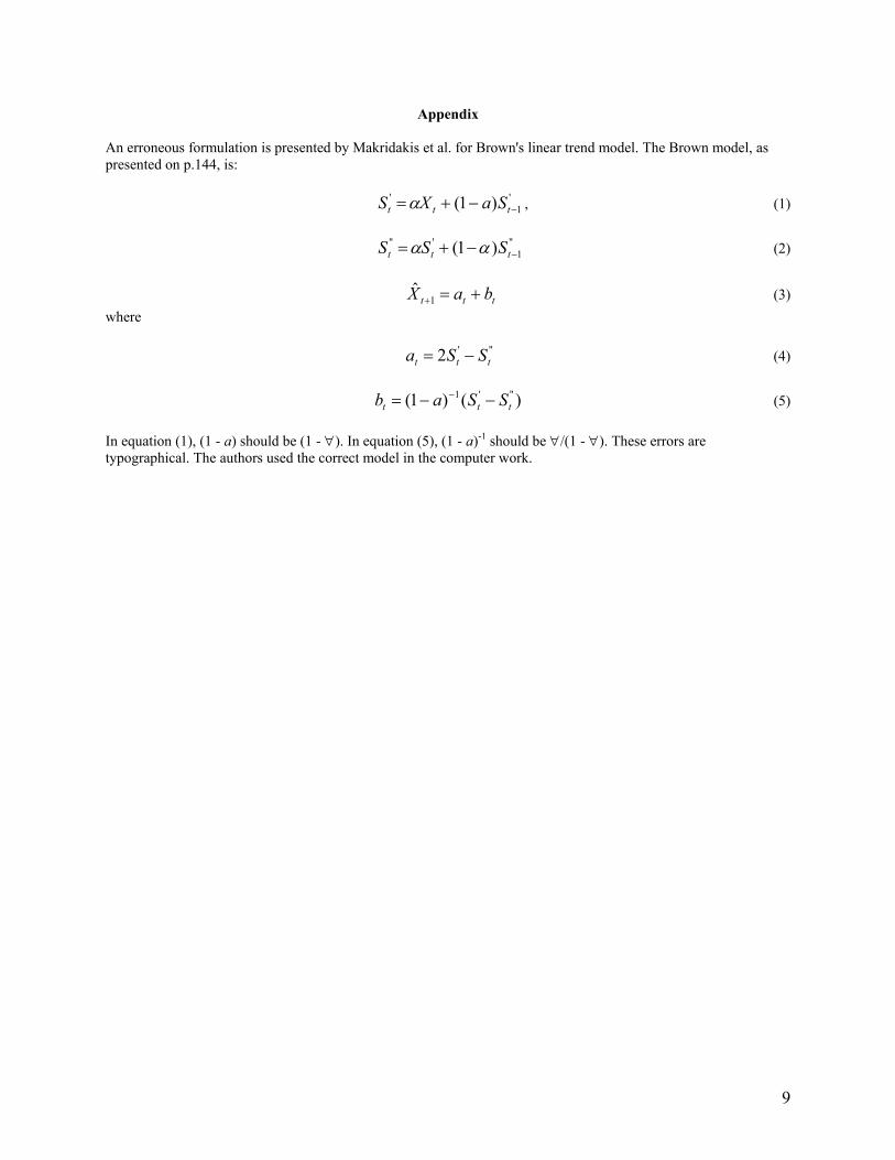
Appendix An erroneous formulation is presented by Makridakis et al. for Brown's linear trend model. The Brown model, as presented on p.144, is:

'1

' )1( −−+= ttt SaXS α , (1)

"1

'" )1( −−+= ttt SSS αα (2)

ttt baX +=+1ˆ (3)

where

"'2 ttt SSa −= (4)

)()1( "'1ttt SSab −−= − (5)

In equation (1), (1 - a) should be (1 - ∀). In equation (5), (1 - a)-1 should be ∀/(1 - ∀). These errors are typographical. The authors used the correct model in the computer work.

10

Evaluating a Forecasting Competition with Emphasis on the Combination of Forecasts

Michael D. Geurts Business Management, Brigham Young University, U.S.A.

The M-Competition extends the work of Makridakis and Hibon (1979), whose paper is the best forecasting

article I have read in the last ten years. In the same issue, the original article was criticized and commented on by several outstanding scholars. The M-Competition has substantial changes that add to the prior work. It incorporated several of the suggestions made by the discussants of the 1979 paper, but it failed to deal completely with some suggestions. Both articles are a replication and extension of the widely cited paper by Newbold and Granger (1974).

The Case For Box-Jenkins

The Box-Jenkins forecasting method has received an enormous amount of attention in the academic literature. A prevalent assumption of the literature was that Box-Jenkins was the best forecasting technique. In contrast to the assumptions and findings of Newbold and Granger (1974), the M-Competition and Makridakis arid Hibon (1979) show Box-Jenkins to be inferior to many other forecasting methods.

One possible explanation of the conflict in findings between Newbold and Granger (1974) and the two

Makridakis papers is that exponential smoothing is a “mechanical” process, whereas Box-Jenkins requires insight and experience to identify the ARIMA underlying process. It is possible in the Box-Jenkins forecasting that the forecaster did not identify the “right” underlying process. In fact, it is probable for two experienced Box-Jenkins forecasters to examine the same autocorrelations, partial autocorrelations, and spectral density estimates, and then to specify different models. The supposition remains that the “best” Box-Jenkins model was not selected for each time series in the current study; but then one could make, such an argument for any competition. In its defense, the M-Competition tried to reduce the criticism of the wrong Box-Jenkins specification by examining the lag residual autocorrelation with the Box-Pierce X statistic.

The conflict with the Newbold and Granger paper could also be the result of Newbold and Granger's using

an inferior exponential smoothing model, or they may have selected a sample of time series that are best forecasted with ARIMA models. In an attempt to solve this problem, the Makridakis projects used two different exponential smoothing models. To eliminate the conflict, the Newbold and Granger procedure could be replicated using the 1001 data series.

The Criteria For Accuracy

Three of the major contributions of the article are its evidence that (1) there is no “best” forecasting technique, (2) the best technique changes from one forecasting horizon to the next, and (3) the best technique changes when different measures of accuracy are used.

A discussion of the advantages and disadvantages of different criteria is given by Makridakis and Hibon

(1979). A criterion used in this study, but not in the 1979 study, was average ranking. Interestingly, for this accuracy measure, combining method A has the lowest value (most accurate) for every time horizon (see Table 4(a) in the M-Competition).

Gilchrist (1979) discussed the problem of averaging the accuracy measure for several time series. This

procedure may mask the ability of some models to forecast some types of time series better than others. In the M-Competition, the time series are categorized and an analysis of errors is carried out for each category. Although this is a substantial improvement over the prior procedure, it is still possible that the best method in a category may not be the best method for an individual case, or that the categories are not properly defined.

The M-Competition did not discuss the problem of averaging MSE across time series. MSE is an excellent

measure of accuracy for evaluating an individual time series. However, it is not useful in an averaging process for several time series; distortion can occur because of the different magnitudes of each series. For example, two widely forecasted time series are the unemployment rate and GNP. Because of the difference in magnitude of the two time

11

series, the average of the mean squared errors favors the model that forecasts GNP best. In other words, a few series might dominate the averages.

Makridakis and Hibon (1979) used the U statistic to evaluate forecasting accuracy. U is a ratio

measurement with MSE as the numerator. This procedure facilitates averaging and removes the problem discussed above. It would have been useful for the M-Competition.

One significant finding in the M-Competition, in contrast to the findings of the 1979 article, is the accuracy

of the naive model (see Tables 5, 7 and 8). In the earlier article, the naive model compared favourably with the other models; however, in the current article, that is not the case (see Tables 5(a), 6(a), 6(b), 7(a) and 7(b)). This might be attributed to the second study's using some forecasting models that were not used in the first study.

The Use of Combinations of Forecasts

The M-Competition included a combination of forecasts that was not used by Makridakis and Hibon

(1979). The combination was, in many cases, the “best” model. In Table 4(a), combining technique A had the lowest average error ranking for the 1001 set. This was true for the forecasts of t + 1 to t + 12 time periods. It also had the lowest MA PE in Table 2(a) for the 1001 time series for many of the forecasted time horizons.

The question addressed in the M-Competition was “What is the best forecasting model?” The answer, from

the empirical research, is the use of a combination of forecasts. A combining technique will usually outperform an individual model. (Editor's note: See Gardner's Commentary and Winkler's Reply for additional viewpoints on this issue.) This raises a new question: What is the best method of combining forecasts? Other combining techniques might produce greater accuracy than the procedures followed in the M-Competition.

Combining technique A was simply the average of forecasts from six models (five exponential smoothing

models and one similar model). The difference is that the weights of past data in the forecasting equation are not necessarily confined to an exponential weighting scheme. Why were ARARMA, FORSYS, Bayesian, and Box-Jenkins excluded from the combination model?

Combining method B used the same six forecasting methods, but weighted the forecasted values based on

the sample covariance matrix of percentage error. I was surprised to find that the combining method B performed less effectively than the equal weighting

combination of method A. If equal weighting were the optimum weighting scheme, then the weights based on the sample covariance should have, in fact, generated the equal weighting scheme.

The combining method might be at a disadvantage because of the inclusion of the single smoothing

forecast, as it performs poorly when trend is present in the time series. It would be interesting to see the combining results with the single smoothing method replaced by the Box-Jenkins or Bayesian methods.

In previous work, the combining of forecasts nearly always improved accuracy (e.g. Bates and Granger,

1969). Newbold and Granger (1974) proposed five weighting techniques; why didn't the researchers in this article try one of these? Bunn (1979) suggested a conditional probability combination technique. Reinmuth and Geurts (1979) suggested using a regression technique, in which the regression coefficients are determined using past actual sales as the dependent variable, and forecasts of different models as independent variables.

12

Pattern, Pattern-Who's Got the Pattern?

LOLA L. LOPES University of Wisconsin, Madison, U.S.A.

Forecasting methods are rather alien turf for cognitive psychologists. Nevertheless, the results of the

M-Competition have caused this cognitive psychologist to wonder whether there might be important similarities between the problems of extrapolative forecasting and certain cognitive problems in ordinary living.

One of the most vital capacities that people have is the ability to learn from experience. Such learning rests

on the ability to distinguish between noise (i.e. randomness) and pattern (i.e. nonrandomness). Gregg Oden and I (Lopes, 1982; Lopes and Oden,1981) have been studying how people's beliefs about randomness affect their proficiency at making this discrimination. The task we have used requires people to judge whether a given event has been produced by a random or a non-random process. To be sure, this cannot be done perfectly, but the judgment situation is not radically different from any situation in which a signal must be discriminated from a noisy background (Green and Swets, 1966).

In our experiments, we varied the type of non-randomness subjects had to detect, and the instructional

conditions under which they worked. Subjects were shown 500 8-character binary strings. They were told that half of the strings would be generated by a random process and half would be generated by a non-random process. The random process was a Bernoulli process with p= 0.5. The non-random process was a stationary Markov process with a repetition probability of 0.8 for the `repetition-biased' condition, and 0.2 for the alternation-based condition. We were particularly interested in the alternation-biased condition since statistically naive people have been shown to have a misconception about randomness that should make alternation especially hard to detect. Specifically, they expect that random strings will alternate more often (i.e. have fewer runs) than they really do (Wagenaar, 1972).

Our instructional manipulation involved how much we told people about the non-random process. In the

“uninformed” condition, subjects were simply told that the process was non-random, and left to their own interpretations: In the “informed” condition, subjects were told that the process had a tendency either to repeat symbols (for the repetition-biased condition) or to alternate symbols (for the alternation-biased condition). In the feedback condition, subjects were given no instruction concerning the non-random process, but after every trial were informed about which process had generated the string.

In a nutshell, our results were: First, the alternation-biased condition was, indeed, more difficult than the repetition-biased condition, particularly when subjects were uninformed. Second, both minimal instruction and feedback were effective in improving subjects' performances, particularly for subjects in the alternation-biased condition.

What has this to do with extrapolative forecasting? The connection I see is that experts who design

forecasting systems are much like subjects in the uninformed conditions of our experiments: they must find ways to discover patterns in noisy data without knowing what kind of pattern to expect. For naive subjects, a critical variable affecting performance is whether their concepts of pattern and noise are in tune with the kind of non-randomness that is actually there. I would expect a similar situation to hold for extrapolative forecasting methods.

Do Programs Have Beliefs? Should Programs Have Beliefs?

Although programs in artificial intelligence are sometimes claimed to have beliefs, I do not think that statistical programs are ever viewed in that light. Nevertheless, it is clear that the people who create programs have beliefs, and it is not too far-fetched to suppose that their programs implicitly embody some of these beliefs.

As McLaughlin points out in his commentary, Naive 1 has the simplest belief possible: the world will be

the same tomorrow as it is today; everything is pattern, nothing is noise. Methods like the simple moving average and single exponential smoothing have somewhat more sophisticated beliefs: the world will be similar tomorrow to what it is today; part is pattern, part is noise. Still other methods have more complicated beliefs about seasonality and trends.

13

Thinking of forecasting methods as having something like implicit beliefs makes it easier to understand why the sophisticated methods did not, in general, outperform the simpler methods. Suppose that among the 1001 time series there are many kinds of pattern represented. For those series in which the implicit beliefs of the sophisticated methods are appropriate, the methods would, presumably, do well; but for series in which the beliefs are inappropriate, the sophisticated methods would fall behind simpler methods that embody less sophisticated but more universally applicable notions of pattern and noise.

In his commentary, Newbold questions whether automatic methods will produce real forecasts without

having a thinking human being serve as the “front end” of the system. But it also seems reasonable to ask whether there are some “front end” functions that might be automated by giving forecasting programs some of the beliefs that knowledgeable forecasters bring to their art.

Two classes of beliefs seem pertinent. The first class are generalized beliefs about what time series are like.

For example, Newbold says that sensible forecasters will graph their data and look for outliers before doing anything else. Presumably they also gauge the variability in the data and get some idea about the overall shape of the series. I see no reason, in principle, why forecasting programs cannot be “taught” to do these things also. Perhaps they will never do them as well as human beings, but they might at least screen series and flag those that seem to require the services of a human forecaster.

The second class of beliefs that might be embodied in forecasting programs are substantive beliefs about

the system that generates the data. Of course, the M-Competition concentrated on exactly those methods that do not make use of causal factors—in other words, on methods that are designed for use in the “uninformed” condition. Nevertheless, given the obvious advantages of knowing something about the patterns to be expected, it seems that extrapolative methods would be strengthened by making provision for causal or explanatory information to be used, when such is available.

I grant that the forecasting programs I envision are artificial intelligence systems and not mere “number

crunchers,” but why not? The sensible forecasters that Newbold describes are in the “informed” condition, so to speak. Why not inform the extrapolative systems as well?

Recursive Analysis

The 34 tables of the M-Competition illustrate the formidable problems of analysing analyses. We learn, as did the sorcerer's apprentice, the limits of our ability to control and comprehend the massive number-generating power that the computer has given us. What is signal, what is noise? Are we going to need yet another computer program to tell us what these 34 tables mean?

Scott Armstrong asked me to comment on whether people are likely to see patterns in these data even where none exist. The question is a good one since, indeed, people do seem to be biased toward seeing patterns. (I have argued elsewhere (Lopes, 1982) that this bias makes sense in our noisy world.) In the present case, however, I am hard pressed to see that people would discover any patterns at all. The pattern-finding process seems often to rest on perceptual cues: we see a curvature in a graph, we hear a rhythm in music. Tables of numbers strip these cues away. For example, one expects forecasting errors to increase as the forecasting horizon gets larger; but how does error grow—linearly, exponentially, as an ogive? Numbers, as symbols, do not encode these relationships directly; thus, we cannot simply “notice” how the errors grow. Instead, we must slowly and explicitly decode the numbers,, checking their values against previously formed hypotheses. The task is hard enough when the numbers are small and written in F-format, as they are in Table 2(a). When the numbers are large and come in tightly packed arrays of F-format, as in Table 3(a), the mind boggles.

Although I do not think that the data of the M-Competition lend themselves to the easy discovery of facts

about forecasting, I think they will be useful if viewed as a database against which forecasters can test the hypotheses and intuitions gleaned from actual practice. For example, the M-Competition noted that a common belief among economic forecasters was that forecasting became more difficult after 1974. The data, however, did not support this belief. Why was this belief so widespread, and why was its falseness not noted before?

14

One possible explanation is that forecasters were misled by an accident of the causal labels they applied to forecasting errors before and after 1974. Presumably, forecasts that failed before 1974 were attributed to a variety of factors; after 1974, however, instability in the price of oil was likely to be cited as an important cause in almost every forecasting failure. This uniformity in causal labeling may well have increased the salience and retrievability of failure in general, making forecasting seem to be more difficult after 1974 (cf. Tversky and Kahneman,1973). I suspect that the impressions we form of whether a pattern-finding method is doing well or poorly depend on the kinds and diversity of “reasons” that we can call upon to account for failures. Given a salient causal theory to “explain” our failures, we may be more likely to detect a pattern in errors, whether one exists or not.

Detecting patterns against noise is a difficult task, made doubly so when, as is the case with economic

forecasting, we cannot even be sure that there is a pattern to be detected. Whether or not we do well depends, at least in part, on a complex interaction between (1) how we define patterns generally, (2) the particular kind of pattern that we expect to find in a given body of data, and (3) the particular kind of pattern that is actually there. Sometimes it is easy to discover patterns even when none exist (Cole, 1957; Slutzky, 1937). At other times the process is made difficult simply because we are looking for the wrong sort of pattern; but despite the difficulties, people seem to do pretty well, as do the forecasting methods they devise.

15

Does the M-Competition Answer the Right Questions?

Robert E. Markland University of South Carolina, U.S.A.

During the past two decades a large number of extrapolation methods have been developed, tested, and

used for forecasting. As each forecasting method has been introduced, there has been a tendency to claim superiority for it, even though it has not yet been tested against other methods in a variety of forecasting situations. Consequently, one is uncertain as to what forecasting technique to use for a particular problem. Makridakis and his group of distinguished forecasting experts are to be congratulated for their comprehensive work concerning the value of specific forecasting methods for particular forecasting situations.

The M-Competition takes a major step towards the much needed broad-based comparison of major

extrapolation methods. It is hoped that its approach and results will encourage further work. The M-Competition benefits practitioners in that it provides a comprehensive evaluation of the accuracy of

a wide range of time series methods in different situations. For researchers, it provides a structure for comparing research methods in a rigorous manner. In addition, provision has been made so that most of the results of this study can be replicated (i.e. the authors will provide computer tapes of the forecasting data tested and computer programs for the forecasting methods and accuracy measures used).

Scope and Nature of the M-Competition

The scope and nature of the M-Competition seem appropriate for the task of deciding which method is most useful in a given situation. They forecasted 1001 time series for six to eighteen time horizons. Although 24 extrapolation methods were tested, and this reviewer could find no important extrapolation method omitted, it may be possible to suggest others. This evaluation is the most exhaustive undertaken to date in terms of the number and variety of extrapolation methods considered.

The accuracy measures employed in comparing the forecasting techniques were also comprehensive. Five

commonly used accuracy measures were computed for each of the time series tested, by each of the forecasting methods. Although the analysis was fairly complete, a coefficient of variation should have been included as a way of facilitating comparison of forecasting results for time series of widely varying magnitudes.

The discussion on the time and cost of running the various forecasting methods was unsatisfactory. It

mentioned only that the Box- Jenkins methodology required the most computer time, and that the Bayesian forecasting procedure required five minutes of an expert's time to decide on the model to be used for each set of data. Computational times or costs were not provided. In my experience in business and government environments, computer time requirement is an important factor in the choice of a forecasting method to be employed. This is especially important in cases where accuracies are comparable, as they were in this study. A summary table on the times and costs for each of the forecasting methods would be desirable.

Interpretation of the Results of the M-Competition

The interpretation of the results of the M-Competition was difficult for me. Initially, the authors presented 40 detailed tables, each with five summary measures of accuracy for each of the forecasting methods. The authors suggested that “the best way to understand the results is to consult the tables carefully.” Only the most dedicated researcher (or perhaps an insomniac) would be likely to do so. The tables are difficult to interpret and understand. Although the M-Competition provided some observations on the performance of the various forecasting methods, I would have preferred a more extensive yet concise summary.

I agree with the authors that there is no one single method that can be used across the board. The forecaster

must consider the time horizon, whether micro or macro data are being forecast, and whether or not seasonality is important.

16

Further analysis of these data and of the forecasting errors may offer insight on the choice of the most appropriate method for each situation.

17

Forecasting Models: Sophisticated or Naive?

Robert L. Mclaughlin Micrometrics, Inc., Cheshire, CT 06410, U.S.A.

The M-Competition is a landmark which we will be studying for years to come. This contribution has

provided excellent material for analyzing extrapolative forecasting methods; but the study cries out for a measure of accuracy that has been available for a long time: what percentage of total change does the forecaster successfully predict?

The Naive Models

In the 1940s, economists suggested “naїve models” as benchmarks of forecasting accuracy. The basic naїve model, known as “Naїve Forecast 1” or simply “NF 1” is defined thus: the next period's level will be the same as that of the preceding period. If our forecasting model cannot do better than NF 1, it should be disqualified. NF 1, then, becomes the benchmark of the worst permissible error. NF 1 can be said to be the ultimate forecast error measurement.

Naїve Forecast l has a long history. Indeed, we might credit its origin to the caveman who predicted that “tomorrow's weather will be the same as today's;” but, if we delve into the literature of forecasting, the earliest documentation belongs to W. Braddock Hickman of the National Bureau of Economic. Research, who, in 1942, built a naive model test (Hickman,1942).1 In 1949, at the National Bureau Conference on Business Cycles, the idea was discussed by Milton Friedman (Christ, 1951). He suggested that no one would take na1ve models as serious forecasting models. Rather, they provide standards of comparison. His comments about NF 1 are universally applicable to forecasting models

. . . The essential objective behind the derivation of econometric models is to construct an hypothesis of economic change; . . . given the existence of economic change, the crucial question is whether the theory implicit in the econometric model abstracts any of the essential forces responsible for the economic changes that actually occur. Is it better that is, than a theory that says there are no forces making for change? Now naїve model 1. . . denies, as it were, the existence of any forces making for changes .... If the econometric model does no better than this naїve model, the implication is that it does not abstract any of the essential forces making for change; that it is of zero value as a theory explaining change. (Friedman, 1951)

Forecasters hope to anticipate change. The U.S. Census Bureau measures change as the “percent change

from the preceding period, averaged without regard to sign.” The computation could not be simpler—if we had a +10 percent change one month and a -10 percent the next, average change ignoring the signs would be 10 per cent. The fact that volume does change is what makes forecasting interesting.

One of the most common ways to calculate forecasting errors is the “percentage error”—if we forecast 100

and the actual turns out to be 110, our error is +10 per cent. Using NF 1, if our latest actual sales level was 100, we predict 100 for the next period. The actual 110 means a 10 per cent change and NF 1 failed to predict any of it. Thus, if NF 1 is a no-change forecast, then actual change is also the error when NF 1 is a forecasting model. Thus, if NF 1 produces an average error of 10 per cent and our error using some other model averages 8 per cent, the latter model forecasted 20 per cent of the total change. CHANGE VERSUS ERROR

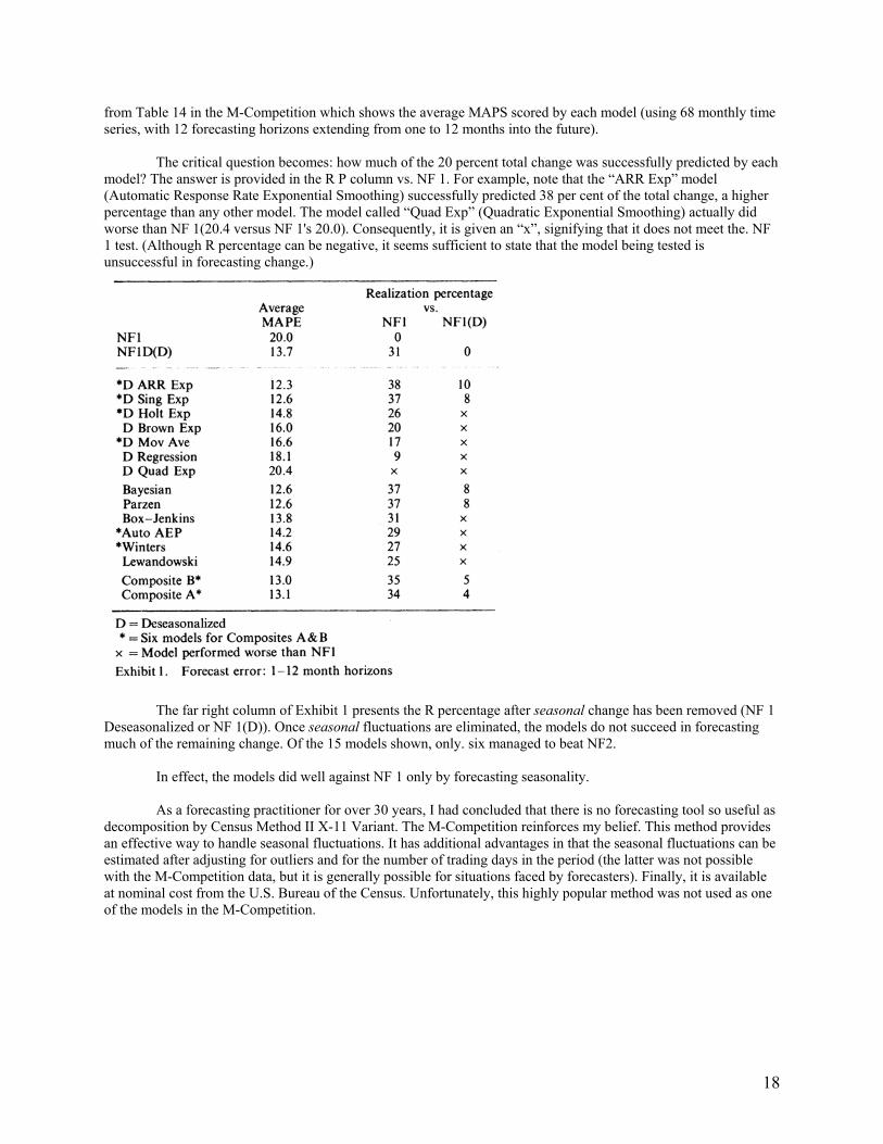
Exhibit 1 provides three measures of forecast error. The second column, the Mean Absolute Percentage Error (MAPS), represents the base data for calculating each “realization percentage” or “R percentage” (proportion of total change successfully predicted) for several of the models shown in the M-Competition. These data come

1 The author is indebted to Dr. Geoffrey H. Moore for help in documenting the historical development of the “naїve models.”

18

from Table 14 in the M-Competition which shows the average MAPS scored by each model (using 68 monthly time series, with 12 forecasting horizons extending from one to 12 months into the future).

The critical question becomes: how much of the 20 percent total change was successfully predicted by each

model? The answer is provided in the R P column vs. NF 1. For example, note that the “ARR Exp” model (Automatic Response Rate Exponential Smoothing) successfully predicted 38 per cent of the total change, a higher percentage than any other model. The model called “Quad Exp” (Quadratic Exponential Smoothing) actually did worse than NF 1(20.4 versus NF 1's 20.0). Consequently, it is given an “x”, signifying that it does not meet the. NF 1 test. (Although R percentage can be negative, it seems sufficient to state that the model being tested is unsuccessful in forecasting change.)

The far right column of Exhibit 1 presents the R percentage after seasonal change has been removed (NF 1 Deseasonalized or NF 1(D)). Once seasonal fluctuations are eliminated, the models do not succeed in forecasting much of the remaining change. Of the 15 models shown, only. six managed to beat NF2.

In effect, the models did well against NF 1 only by forecasting seasonality. As a forecasting practitioner for over 30 years, I had concluded that there is no forecasting tool so useful as

decomposition by Census Method II X-11 Variant. The M-Competition reinforces my belief. This method provides an effective way to handle seasonal fluctuations. It has additional advantages in that the seasonal fluctuations can be estimated after adjusting for outliers and for the number of trading days in the period (the latter was not possible with the M-Competition data, but it is generally possible for situations faced by forecasters). Finally, it is available at nominal cost from the U.S. Bureau of the Census. Unfortunately, this highly popular method was not used as one of the models in the M-Competition.

19

The Competition to End all Competitions

Paul Newbold University of Illinois, Champaign, U.S.A.

When I was asked by Scott Armstrong to comment on the M-Competition, I assumed this was because I

had once co-authored an article on methods of forecast evaluation (Granger and Newbold, 1973). However, upon consulting Armstrong (1978b), it emerged that this was an article that need not be read. This left the possibility that since, in Newbold and Granger (1974), I had organized, on a far more modest scale than this, a “forecasting competition,” I might be expected to be sympathetic to such enterprises. This expectation is not entirely justified. However, Newbold and Granger (1974), together with Makridakis and Hibon (1979) are particularly relevant in the present context, as each was published with a lively discussion. These discussions are worth reading, as many of the points made could apply to the present paper.

In commenting on any paper, the first task is to decide what it is all about. In the present instance, this is

not obvious. The title tells us that we are to learn the “results of a forecasting competition.” Yet, early in the introduction, we are cautioned, sensibly, about naively looking for “winners” and “losers.” However, much of the remainder of the paper is devoted to the “horse race” promised in the title. Perhaps the best tack is to ask what can be learned from the paper, leaving aside the thorny question as to what the authors believed its objective to be. The remainder of my comments will be directed along that avenue.

Before beginning a detailed commentary, I must express my admiration for a group of authors who set out

on such an enormously difficult and time-consuming enterprise. This massive task would have appeared so overwhelmingly daunting that many would have shied away from it. Thus, any subsequent criticism of details of the study must be conditioned by the observation that, not only would I refrain from claiming to be able to do better, but also I doubt whether I would have the stamina or the fortitude, not to mention the inclination, to make the attempt.

That the organization of this competition was time consuming is obvious, even from a casual reading of the

paper. There are tremendous difficulties, not only in problems of organization, but also in trying to synthesize and report the huge amount of numerical results generated. I am not at all convinced that this last problem is soluble. Such is the scale of the present enterprise, that it might be labeled “the forecasting competition to end all forecasting competitions.” I suggest later that this would be a desirable outcome.

Before providing a summary of their findings, the authors discussed certain classifications of forecasting

approaches. I urge a further classification, namely approaches where the forecasters think (about the subject matter area, the data, and anything relevant) and those where they do not. Now, in the real world, I claim that forecasters do think about the series they want to predict. Surely, no one seriously considers generating important forecasts without thought. Even when sales forecasts of a large number of product lines are required for inventory control, the analyst will have some experience of what has worked well in the past, and can look rather carefully at a small sample of the series to be predicted. This being the case for realism, we should not deny the forecaster the right to think. Yet, in this study, for 22 of the 24 approaches, “the various data series were put in the computer, and forecasts were obtained with no human interference.” Do practitioners, charged with the responsibility of producing real forecasts, operate this way? I doubt it. Certainly, I believe they should not. Thus, because the competitive methods are not approaches used in practice, is the comparison not one of “irrelevant alternatives?” We should distinguish carefully between approaches to forecasting, and forecasting methods. I have already argued that individuals approaching a forecasting problem will not deny themselves the right to think. On the other hand, I know that there are forecasting methods that automatically produce predictions of future values of any time series. I know this because I have computer programs into which I can read a data series, and out of which will emerge predictions. Many of these programs require no further information, and, indeed, are incapable of using it. Now, I am not arguing that sensible forecasters will never use such methods. However, surely, before doing so, they will think carefully, considering the data and the environment, about whether this is appropriate. For example, for any number of reasons, not the least of which is a concern about outliers, it is sensible to graph the data against time before doing anything else. Yet, in this competition, even for the approaches where some thought was permitted, it appears that prior examination of the plotted series was not done. Perhaps this conjecture is not correct. It would be interesting to learn from the authors whether they plotted the series, and in what way their subsequent analyses were modified after examination of the graphs.

20

The reservation in the previous paragraph is far from trivial. However, taking the study on its own terms,

the next question that arises is how to evaluate the competitive methods. Here the authors attempt an array of possibilities, presumably on the grounds that no single cost of error function is appropriate for every problem. Consequently, aggregate comparisons are difficult to make. One interesting question concerns the use of absolute forecast errors. Why, if this is the relevant standard, do we use least squares in estimating model parameters? Also, I am concerned about the comparisons of mean squared errors of prediction in Tables 3(a) and 3(b) of the M-Competition. The reported quantities appear to be mean squared errors, averaged over all series. Such comparisons are not scale-invariant, in the sense that, if we multiplied all the observations in some of the series by 1000, different relative values would be found for these averages. It is for this reason that, in Newbold and Granger (1974), we looked at empirical distributions of ratios of mean squared errors for a pairwise comparison of the performances of forecasting methods.

The authors deserve our thanks for providing so much of the numerical output. However, I feel that a more

concise synthesis would also have been valuable. The injunction “that the best way to understand the results is to consult the various tables carefully” leaves us a lot of work to do. Presumably, the authors have already consulted the tables carefully. It would have been helpful had they devoted a little more space to telling us what they learned from doing so. (Editor's note:this is accomplished in the `Reply' where each author presents personal conclusions.) Of course, given any set of data, we are all free to form our own conclusions, but careful synthesis of masses of numerical information is part of the statistician's trade, and more work along these lines might have been useful in the M-Competition. Personally, the most important lesson I learned from careful consultation of Tables 1 to 9 was the value of aspirin.

The summary section, “Some General Observations,” is where I hoped to find a more complete discussion

of what had been learned from the enormous effort in the M-Competition. However, this section of the paper is disappointingly brief, and many of its general conclusions could have been divined without the benefit of such a huge study. For example, it is hardly surprising to learn that the performances of various methods depend on the characteristics of the data and the standard of comparison used. Furthermore, “the greater the randomness of the data, the less important is the use of statistically sophisticated models” is fairly obvious. It would have been interesting here to include a discussion of outliers; this possibility is catered for by just one of the methods examined, Bayesian forecasting, though this possibility would surely not be ignored by approaches to forecasting based on the other methods.

One intriguing question raised in their summary concerns the prior seasonal adjustment of a series before

subsequent analysis. It appears that exponential smoothing of seasonally adjusted series produces good forecasts, compared with methods that attempt explicitly to model seasonality. This being the case, I would conjecture that fitting ARIMA models to seasonally adjusted data would do equally well. I wonder if this was tried. The point was also made by Makridakis and Hibson (1979). Attention was specifically drawn to it by Durbin (1979), who regarded the result as counterintuitive. Certainly, I would support Durbin's plea for more detailed research and exposition on this issue, particularly as we know from the work of Cleveland and Tiao (1976) that the complicated X-11 adjustment procedure can be well approximated by simple members of the seasonal ARI MA class of models.

In this kind of study, it is impossible to draw a random sample of all times series, or a random sample of

series from some identifiable class of interest. Accordingly, formal statistical inference based on the empirical results is not possible. This being the case, it was surprising to see the analysis of variance and other formal tests in the final parts of the paper. The author’s note, in introducing the analysis of variance, that the assumption of normality does not hold true. I wonder, in fact, if any of the necessary assumptions for such an analysis are true.

The second appendix of the paper is valuable. It is extremely useful to have succinct descriptions of all

these forecasting methods, along with references for further details. In our work (Newbold and Granger, 1974), I felt that we had learned more than our readers. This was so

because the paper concentrated on describing the “horse race” aspects of our study. While doing the study, we had the further opportunity to examine individual series in more detail when we found surprising or discrepant results. In doing so, it was sometimes possible to gain more insight into the methods, and to conjecture ways of improving them. For instance, why should ARIMA modeling be seriously out-performed by an exponential smoothing

21

procedure which is really based on a specific ARIMA model, which might have been chosen? Often the answer lay in outlying observations. Ignoring the presence of outliers can lead to the choice of the “wrong” ARIMA structure. Again, we found that rarely, if ever, did the usual portmanteau test indicate model inadequacy, even though many of our initial model identifications were somewhat tenuous. This observation led to the research reported by Davies et al. (1977) and Davies and Newbold (1979) on the small sample properties of this test statistic. It would be extremely useful to hear from the jockeys in this horse race what they learned about their horses. When particular methods performed badly, compared with others, why did this happen? Can modifications be made to pick out and deal with those types of series which cause problems for particular methods? I would this is accomplished in the “Reply” where each author presents personal conclusions.) Of course, given any set of data, we are all free to form our own conclusions, but careful synthesis of masses of numerical information is part of the statistician's trade, and more work along these lines might have been useful in the M-Competition. Personally, the most important lesson I learned from careful consultation of Tables 1 to 9 was the value of aspirin.




subsequent analysis. It appears that exponential smoothing of seasonally adjusted series produces good forecasts, compared with methods that attempt explicitly to model seasonality. This being the case, I would conjecture that fitting ARIMA models to seasonally adjusted data would do equally well. I wonder if this was tried. The point was also made by Makridakis and Hibson (1979). Attention was specifically drawn to it by Durbin (1979), who regarded the result as counterintuitive. Certainly, I would support Durbin's plea for more detailed research and exposition on this issue, particularly as we know from the work of Cleveland and Tiao (1976) that the complicated X-11 adjustment procedure can be well approximated by simple members of the seasonal ARIMA class of models.





because the paper concentrated on describing the “horse race” aspects of our study. While doing the study, we had the further opportunity to examine individual series in more detail when we found surprising or discrepant results. In doing so, it was sometimes possible to gain more insight into the methods, and to conjecture ways of improving them. For instance, why should ARIMA modeling be seriously out-performed by an exponential smoothing procedure which is really based on a specific ARIMA model, which might have been chosen? Often the answer lay in outlying observations. Ignoring the presence of outliers can lead to the choice of the “wrong” ARIMA structure. Again, we found that rarely, if ever, did the usual portmanteau test indicate model inadequacy, even though many of our initial model identifications were somewhat tenuous. This observation led to the research reported by Davies et al. (1977) and Davies and Newbold (1979) on the small sample properties of this test statistic. It would be extremely useful to hear from the jockeys in this horse race what they learned about their horses. When particular methods performed badly, compared with others, why did this happen? Can modifications be made to pick out and deal with those types of series which cause problems for particular methods? I would this is accomplished in the “Reply” where each author presents personal conclusions.) Of course, given any set of data, we are all free to form our own conclusions, but careful synthesis of masses of numerical information is part of the statistician's trade, and more

22

work along these lines might have been useful in the M-Competition. Personally, the most important lesson I learned from careful consultation of Tables 1 to 9 was the value of aspirin.




subsequent analysis. It appears that exponential smoothing of seasonally adjusted series produces good forecasts, compared with methods that attempt explicitly to model seasonality. This being the case, I would conjecture that fitting ARIMA models to seasonally adjusted data would do equally well. I wonder if this was tried. The point was also made by Makridakis and Hibson (1979). Attention was specifically drawn to it by Durbin (1979), who regarded the result as counterintuitive. Certainly, I would support Durbin's plea for more detailed research and exposition on this issue, particularly as we know from the work of Cleveland and Tiao (1976) that the complicated X-11 adjustment procedure can be well approximated by simple members of the seasonal ARI MA class of models.





because the paper concentrated on describing the “horse race” aspects of our study. While doing the study, we had the further opportunity to examine individual series in more detail when we found surprising or discrepant results. In doing so, it was sometimes possible to gain more insight into the methods, and to conjecture ways of improving them. For instance, why should ARIMA modeling be seriously out-performed by an exponential smoothing procedure which is really based on a specific ARIMA model, which might have been chosen? Often the answer lay in outlying observations. Ignoring the presence of outliers can lead to the choice of the “wrong” ARIMA structure. Again, we found that rarely, if ever, did the usual portmanteau test indicate model inadequacy, even though many of our initial model identifications were somewhat tenuous. This observation led to the research reported by Davies et al. (1977) and Davies and Newbold (1979) on the small sample properties of this test statistic. It would be extremely useful to hear from the jockeys in this horse race what they learned about their horses. When particular methods performed badly, compared with others, why did this happen? Can modifications be made to pick out and deal with those types of series which cause problems for particular methods? I would this is accomplished in the “Reply” where each author presents personal conclusions.) Of course, given any set of data, we are all free to form our own conclusions, but careful synthesis of masses of numerical information is part of the statistician's trade, and more work along these lines might have been useful in the M-Competition. Personally, the most important lesson I learned from careful consultation of Tables 1 to 9 was the value of aspirin.


of what had been learned from the enormous effort in the M-Competition. However, this section of the paper is disappointingly brief, and many of its general conclusions could have been divined without the benefit of such a huge study. For example, it is hardly surprising to learn that the performances of various methods depend on the characteristics of the data and the standard of comparison used. Furthermore, “the greater the randomness of the data, the less important is the use of statistically sophisticated models” is fairly obvious. It would have been interesting here to include a discussion of outliers; this possibility is catered for by just one of the methods

23

examined, Bayesian forecasting, though this possibility would surely not be ignored by approaches to forecasting based on the other methods.


subsequent analysis. It appears that exponential smoothing of seasonally adjusted series produces good forecasts, compared with methods that attempt explicitly to model seasonality. This being the case, I would conjecture that fitting ARIMA models to seasonally adjusted data would do equally well. I wonder if this was tried. The point was also made by Makridakis and Hibson (1979). Attention was specifically drawn to it by Durbin (1979), who regarded the result as counterintuitive. Certainly, I would support Durbin's plea for more detailed research and exposition on this issue, particularly as we know from the work of Cleveland and Tiao (1976) that the complicated X-11 adjustment procedure can be well approximated by simple members of the seasonal ARIMA class of models.




these forecasting methods, along with references for further details.

In our work (Newbold and Granger, 1974), I felt that we had learned more than our readers. This was so because the paper concentrated on describing the `horse race' aspects of our study. While doing the study, we had the further opportunity to examine individual series in more detail when we found surprising or discrepant results. In doing so, it was sometimes possible to gain more insight into the methods, and to conjecture ways of improving them. For instance, why should ARIMA modeling be seriously out-performed by an exponential smoothing procedure which is really based on a specific ARIMA model, which might have been chosen? Often the answer lay in outlying observations. Ignoring the presence of outliers can lead to the choice of the “wrong” ARIMA structure. Again, we found that rarely, if ever, did the usual portmanteau test indicate model inadequacy, even though many of our initial model identifications were somewhat tenuous. This observation led to the research reported by Davies et al. (1977) and Davies and Newbold (1979) on the small sample properties of this test statistic. It would be extremely useful to hear from the jockeys in this horse race what they learned about their horses. When particular methods performed badly, compared with others, why did this happen? Can modifications be made to pick out and deal with those types of series which cause problems for particular methods? I would certainly hope to see some discussion along these lines in the forthcoming book, which is to elaborate on the M-Competition.

Finally, I question whether we get the maximum benefit from competitions of this sort, given the amount of

effort involved. More to the point, given what has now been done along these lines, are the marginal benefits to be expected from further such studies high? I think not, and would argue that the development of the art of forecasting would be better served by a concentration of resources elsewhere. Indeed, I believe that much would be gained from a diametrically opposite line of work. In the competitions, a small amount of effort is spent on the analysis of each of a large number of series. The results that are reported are, of necessity, aggregate results, and the forecaster, faced with a specific problem, learns little about how such a problem might be attacked. Suppose, instead, that we were to encourage studies in which a large amount of effort was spent on a single forecasting problem. Good studies of this sort would not be content with the routine application of forecasting methods. Rather, through such case studies, we could learn more about sensible approaches to forecasting problems. I am sure that the Journal of Forecasting could best serve the profession by soliciting, and encouraging the publication of, case studies. Ideally, these should come from practitioners rather than academics, and certainly should be practical rather than academic. In contrast to the competition philosophy, a good case study would inevitably involve a careful discussion of the environment of a specific problem, of all relevant subject matter, theory, and data, and of the specific characteristics of the data at hand. The justification of whatever technical procedures are used to generate forecasts would then be problem-specific, rather than based on aggregate conclusions derived from the analysis of largely unrelated problems.

Space limitations preclude a more detailed specification of the essentials of good case study presentation.

Suffice it to say that, in my view, forecasting is an area in which “learning by case study” is likely to be extremely

24

valuable—far more so, for example, than anything we are likely to learn from further competitions, however grand their scale.

25

What Do These Numbers Tell Us?

David J. Pack Union Carbide Corporation

It is difficult for most readers to appreciate the amount of time invested by the authors of the monumental

M-Competition. Having been an organizer of the 1978 TIMS-ORSA competition, which was based on only four time series, this reviewer knows of the seemingly minor obstacles that become major roadblocks in this kind of endeavour. Whatever else one says, one must give credit to the authors of the M-Competition for their willingness to undertake this enormous 1001 series competition.

I present my commentary on the M-Competition speaking from the three roles my background permits me to adopt in this discussion—that of a statistician, a Box-Jenkins forecaster, and an associate editor of the Journal of Forecasting certainly hope to see some discussion along these lines in the forthcoming book, which is to elaborate on the M-Competition.

Finally, I question whether we get the maximum benefit from competitions of this sort, given the amount of

effort involved. More to the point, given what has now been done along these lines, are the marginal benefits to be expected from further such studies high? I think not, and would argue that the development of the art of forecasting would be better served by a concentration of resources elsewhere. Indeed, I believe that much would be gained from a diametrically opposite line of work. In the competitions, a small amount of effort is spent on the analysis of each of a large number of series. The results that are reported are, of necessity, aggregate results, and the forecaster, faced with a specific problem, learns little about how such a problem might be attacked. Suppose, instead, that we were to encourage studies in which a large amount of effort was spent on a single forecasting problem. Good studies of this sort would not be content with the routine application of forecasting methods. Rather, through such case studies, we could learn more about sensible approaches to forecasting problems. I am sure that the Journal of Forecasting could best serve the profession by soliciting, and encouraging the publication of, case studies. Ideally, these should come from practitioners rather than academics, and certainly should be practical rather than academic. In contrast to the competition philosophy, a good case study would inevitably involve a careful discussion of the environment of a specific problem, of all relevant subject matter, theory, and data, and of the specific characteristics of the data at hand. The justification of whatever technical procedures are used to generate forecasts would then be problem-specific, rather than based on aggregate conclusions derived from the analysis of largely unrelated problems.

Space limitations preclude a more detailed specification of the essentials of good case study presentation.

Suffice it to say that, in my view, forecasting is an area in which `learning by case study' is likely to be extremely valuable—far more so, for example, than anything we are likely to learn from further competitions, however grand their scale.

From A Statistician The problem of numeracy

Tables 1 to 34 of the published results contain approximately 17,000 numbers (exactly 16,710 numbers excluding zero-fillers, but you won't remember the exact figure). What do these numbers tell us? Most readers probably will concede defeat in their attempts to draw inference from these tables.

The problem of numeracy is defined by Ehrenberg (1981):

Lack of numeracy is due mainly to the way data are presented. Most tables of data can be improved by following a few simple rules, such as drastic rounding, ordering the rows of a table by size, and giving a brief verbal summary of the data.

The M-Competition provided an outstanding example of the problem of numeracy.

26

Consider Exhibits 1 and 2. Exhibit 1 is a straight reproduction of the paper's Table 2(b). Exhibit 2 is the

same table with methods ordered to the “average of forecasting horizons 1-12” column and all MAPE's divided by 13.4, the minimum MAPE in the ordering column. All Exhibit 1 numbers are available from Exhibit 2 after a simple multiplication. But much more is available, including at least the following:

(a) a clearer picture of which methods performed better as judged by the MAPE for the 111 series sample

(b) a perception that the poorer methods in average 1-12 MAPE terms deteriorate even more relative

to other methods at lead times of 15 and 18

(c) innumerable simple ratio comparisons, method to method, or horizon to horizon.

27

The cost of going to Exhibit 2 is the somewhat arbitrary selection of the ordering column and the increased difficulty of finding results for a specific method of interest. These costs are well worth the sense of order that flows from Exhibit 2. The properties of forecast accuracy statistics

The M-Competition's discussion of sampling variation in forecast accuracy statistics (MAPS, MSE, etc.), focusing on Table 10, is a necessary beginning to substantial research into the properties of these statistics. Such research is required before empirical forecast comparisons can attain their full value.

Before considering variation, one must consider central tendency. The average-over-horizon statistics of

Exhibits 1 and 2 clearly mix apples and oranges in terms of statistical expectation, or mean value. The single horizon statistics are argued by Jenkins (1982) to involve another mixing of expectations by averaging over different time series. We must seek an accommodation between intuitively appealing statistics and expectationally sound statistics.

Considering variation, let us focus on the MSE (mean square error) forecast accuracy statistic, which is the

preferred accuracy statistic according to the Carbone-Armstrong (1982) survey. Makridakis et al. state that “in general, the MSE fluctuates more than the other measures.” This observation is based on MSEs averaged over all time series in the competition for forecasts from one time origin at individual lead times of 1,2,4,6,8,12,18 and averaged over lead time groups 1-4, 1-12 and 1-18.

This writer (1982) recently studied MSE fluctuation in depth in the context of the ARIMA methodology and the

specific example of the Box-Jenkins (1970) airline passenger data model. The findings were

I. Individual lead time MSEs had coefcients of variation of 1.30,1.35,1.38,1.39,1.40,1.40 and 1.41 for individual lead times 1, 2, 4, 6, 8, 12, 18 respectively.

II. Individual lead time MSEs for forecasts from the same fixed time origin were highly positively correlated. III. Because of II, above, averaged-over-lead-time MSEs did not yield the degree of reduced variability one

normally expects to result from an averaging process. IV. MSEs for different forecast time origins and a fixed lead time will be uncorrelated if the difference in time

origins is at least as large as the fixed lead time.

The possibilities for uncorrelated MSEs for different forecast time origins are shown in Exhibit 3. It contains average-over-lead-time MSE statistics for the airline passenger data for forecasts at seven separate time origins produced by the model Box and Jenkins (1970) describe in their Chapter 9.

The findings quoted above and Exhibit 3 imply a tremendous potential MSE variability in the context of the ARIMA methodology. They direct us to design comparisons around multiple time origins in preference to the M-Competition's design of multiple lead times around a fixed time origin. The direction they give us is important, and such findings need to be generalized to other forecast accuracy statistics and other methodologies.

Exhibit 3. Box-Jenkins airline passenger MSEs (10s) for selected lead time groups at multiple time origins Lead times Time origin Ratio max to min 102 103 104 105 106 107 108 1-12 138 164 196 168 127 123 83 2.4 13-24 363 410 497 367 262 225 101 4.9 25-36 515 574 747 568 404 366 198 3.8 1-24 251 287 347 267 195 174 92 3.8 1-36 339 383 480 368 264 238 127 3.8

28

From A Box-Jenkins Forecaster

What do those of the ARIMA model building school developed by Box and Jenkins think of their method vis-a-vis other methods, empirical comparisons, and related issues? First, be assured that we would accept without reservation and further emphasize the following statement in the M-Competition results paper

It is important to understand that there is no such thing as the best approach or method as there is no such thing as the best car or best hi-fi system. Cars or hi-fis differ among themselves and are bought by people. who have different needs and budgets. What is important, therefore, is not to look for “winners” or “losers” ....

Those who assume a position of uniform superiority should be ignored.

Next be assured that we make no apologies for taking an hour or more to develop a set of forecasts for a single series, or for requiring “human interference” in the process. Sometimes the need is to forecast 1001 substantially different series in two months, and that is a need we cannot readily fulfill. But sometimes the need is to forecast a few very important series in a week, and that is a need we may fulfill if the historical series are informative. In forecasting these “important series,” forecast errors arising from ignorance of the data are potentially much more costly than the forecaster's time. It would often be ludicrous in these cases to tell your boss that such forecasts were produced in five minutes by a computer lacking the power to consider the individual peculiarities of the forecasting situation. Thus, one should no more imply that speed and absence of human interference are uniformly sought goals than one should imply that there is a uniformly best method.

Finally, the Box-Jenkins forecaster need feel no remorse at not appearing to be a winner in the

M-Competition. First, serious questions remain about the validity of the experimental design in this competition as discussed in the previous section of this commentary and, more generally, by Jenkins (1982). These include a single forecast time origin, averaging over different time series, averaging over lead times, and focusing on a sequence of highly positively correlated lead times.

Second, all time series forecasters must face the reality that many variables cannot be forecast adequately

with any single series approach. In the presence of random variation around a mean, random walk movement, or other forms of uncorrelated movement (beyond simple nonstationarities), ARIMA model building and a theoretically less general approach such as single exponential smoothing are going to look the same—bad! To the extent that the M-Competition contained substantial numbers of these uninformative time series, the comparative accuracy statistics tell us little. A Ford and a Jeep may cover flat ground in about the same manner; but, most people would still like to have a Jeep when they come to the rugged, hilly terrain, and some of us would rather not switch cars in the middle of the trip.

From An Associate Editor Armstrong (1982) established the commitment of the new Journal of Forecasting to good writing and careful refereeing, commitments that are reflected in the “Guidelines for Authors” published on the inside-back cover of each journal issue. These ideals should have been carefully established as real in the M-Competition, an important paper by nine authors including six of the Journal's editors and associate editors. Sadly, I felt the paper fell far short of these ideals. (Editor's note: for a summary of how other commentators felt, see the summary in our introduction.)

My feeling is one of cumulative mediocrity. The paper was not badly written and produced. It just wasn't well written and produced. The unimaginative presentation of the tables, which take up so much of the paper, is a significant part of my discontent. In addition, many individually insignificant problems in the paper led to a disappointing final product. The responsibility for writers and referees is cumulative: all writers are guilty of bad writing and misstatements at times. That is one reason journals have referees. The final published product is the cumulative effort of both writers and referees, and they share the blame, the former publicly, the latter privately.

At the risk of hiding the forest behind the trees, some of the individually insignificant problems from this writer's

perspective are

29

English usage

Page 112, end of paragraph two (“so that forecasting users can be able to make rational choices for their situation”). Page 142, end of paragraph two in the Conclusions (“seasonal variations that dominate the remaining of the patterns”). Statements of the obvious

Page 123 [“The performance of various methods differs considerably sometimes, depending upon the accuracy measure (criterion) being used.”] Page 127 [“It is to be expected that methods which do not take trend into account will not do as well as methods which do for data subject to substantial trends (e.g. yearly).”] Page 127 [“It is believed that the greater the randomness in the data, the less important is the use of statistically sophisticated methods.”] Poor definition MAPS is called mean average percentage error on page 114 and mean percentage error on page 143. Neither term is correct. Ignored “Guidelines for Authors” Reference to “tables” rather than “exhibits.” Formula errors b, bottom page 144. Equation (25), page 145. Confusion of a and d, page 148. Cumulatively, the forest is too big for this paper by these authors in a new journal with lofty ideals.

Summary

The M-Competition paper does not do justice to the enormous effort required in the organization of the data, application of forecasting methods, and calculation of forecast errors and measures of accuracy. The tables are poorly presented, telling the reader little, owing to their lack of numeracy. A cumulatively significant collection of errors and disconcerting statements contribute to a general sense of malaise in this reader and (perhaps unfairly) to a lessening of confidence in the care that may have been exercised in the execution of the quantitative tasks underlying the results.

My attitude toward large empirical forecast comparisons continues on a downward trend that started with the TIMS- ORSA competition of 1978. Other fundamental research must be completed before these comparisons can attain their full value. We must gain a better understanding of the statistical properties of forecast accuracy statistics, including their expectational meaning and their likely variability. These properties will usually be methodology dependent (ARIMA, single exponential smoothing, etc.). These properties will lead to the defensible choice of a comparison's relative emphasis on the components of sample size, forecast time origins, forecast lead times, and forecast time series. These properties will allow the determination of the effective sample size implied by the combination of these components that is required to state that two forecast accuracy statistics in a comparison are significantly different.

30

REPLIES TO THE COMMENTARIES

Viewpoint of the Box-Jenkins Analyst in the M-Competition

Allan Andersen University of Sydney, Australia

Over the last fifteen years, the literature on time series forecasting methods has become substantial. As

soon as one method is proposed, modifications appear. An annoying feature of this, however, is that as each new method is presented, it is accompanied by examples in which the new technique substantially outperforms all others!

As I see it, the most important purpose of comparative papers such as the M-Competition is to provide a

setting in which the well known techniques and proposed techniques can be compared in a controlled way. Never again do we need to see the sunspot or lynx data analyzed merely to demonstrate the superiority of one technique over another. Perhaps now the international airlines data may be retired.

Most of the commentators commented on the summary statistics presented in the published version of the

paper. Some suggest there are too many, whereas others suggest even more comparative statistics. Those presented represent a small subset of possibilities; but those who are sufficiently interested have access to all of the data and all of the competing techniques and thus can compute whatever they want from whatever subset of the series interests them most.

My contribution to the M-Competition is the Box-Jenkins analysis of the 111 series. From the beginning, I

realized that the need for analysis places the analyst in a “no-win” situation as demonstrated in the discussion to Makridakis and Hibon (1979). For this reason, I have decided to spend most of these comments on a discussion of the Box-Jenkins technique as applied in the M-Competition. It is also important to mention that the forecasts presented were a result of the technique, not a combination of the method and the analyst's judgment about future values of each series under consideration. The following steps were performed

(a) The sample autocorrelation and partial autocorrelation functions for various differences of the data were calculated.

(b) From this information a tentative model was formulated. Because the identification package used did not

provide plots, this was the first opportunity to graph the data inexpensively. (c) If the data appeared to be growing exponentially or the residuals from the estimated process seemed to be

correlated with the size of the observations, step (a) above was repeated with the natural logarithm of the data. Unfortunately the software required to do analyses of more complex transformations was not available. Generally, models for both the transformed and untransformed series were produced. The final choice for the set of forecasts was made via an eyeball comparison of the “forecasts” together with the actual values of the historical data, that is the estimation data. The model was checked using tests on the individual autocorrelations and the summary Box-Pierce Chi-square statistic. However, the emphasis was placed on the first few autocorrelations and those at the seasonal lags. Some overfitting was also undertaken. Naturally, one cannot claim that every set of forecasts arose from a model in which all the tests are significant. In fact, it may be better that some models be chosen that fail the tests. However, most models passed these tests, and for those which did not, no reasonable alternative was available. If two models for a particular series were considered, both of which produced insignificant test statistics, a decision on which to use was made on the basis of simplicity and low residual mean squared error. Little attention was placed on significance checks, given the short data series.

(d) Finally, the forecasts were produced in accordance with the symmetrical cost function procedure. Although it

is true that here the forecasts were evaluated using MAPS or APE which are not symmetrical, I am not sure how forecasts that minimize these cost functions are produced. At present, these 111 series are being re-analyzed using, as an estimation criterion, whichever forecast evaluation criterion is chosen.

31

The forecasts were graphed with the data, but the forecasts were not modified unless they became negative, in which case an alternative model was chosen. Newbold is correct in stating that every practitioner would certainly wish to modify an “automatic” process. (Editors note: we believe that every statement containing the word “every” is false.) However, practitioners should be warned against this practice (Granger and Newbold, 1977; Armstrong, 1978b, pp. 248-251). In any case, all the models fitted to the 111 series are available. Some recent work (Andersen, 1983) has shown that it does not matter which of the class of “adequate” models is used with the evaluation statistics used in the M-Competition.

Not surprisingly, I also have a pet measure of forecast error. This one, used by Newbold and Granger

(1974), is the geometric mean-squared one-step-ahead error. If one uses this measure in the M-Competition on the quarterly and monthly series, the results are not substantially different from those obtained by Newbold and Granger (1974). That is, for short term forecasts, the more complex techniques, in particular the Box-Jenkins technique, are a little better; whereas for longer term forecasts it does not really matter which method is used.

32

What can be Learned from the Commentaries?

Robert Carbone University of Laval, Quebec, Canada

In his commentary, Newbold asks what can be learned from the M-Competition. An equally important

question is to ask ourselves what can be learned from the commentaries. My reply will focus on this side of the coin. Having been a participant in the 1978 TIMS-ORSA competition mentioned by Pack, I have experienced the

problems associated with an opinionated evaluation and presentation of results. Fortunately, similar problems have not occurred with the M-Competition. No bitter quarrels have arisen among the participants even though we entered with an interest in winning.

I attribute this lack of friction to the roles assumed by the participants and the organizer. As participants,

we perceived our task as one of providing forecasts, not evaluating their accuracy. In summarizing the results, Makridakis did not insert his judgments. He simply reported results, using a variety of accuracy measures, and this at the request of the participants.

It is true that the information presented is voluminous. However, I do not feel that Makridakis and the

participants failed to synthesize the results. The reader should look at Tables 34(a) and (b). It is better to be accused of lack of synthesis than of presenting, in a complex and biased way, a portion of reality in order to prove a point or confirm a belief. Gardner's commentary confirms that a third person can, indeed, reach conclusions on the basis of the so-called “unimaginative” presentation of results. The tone of the commentaries written by Newbold and Pack attest that they also reached conclusions.

The commentators raise several interesting issues:

(a) Is the M-Competition itself a comparison of irrelevant alternatives? The fact that 22 of the 24 methods

were run under an automatic execution mode does not imply that the comparison is irrelevant. First, the degree of automatism varies from one technique to another. The fact that some methods were performed on all 1001 series and others on only 111 attests to that. This fact alone sets methods apart. Second, as noted by Lopes, automatic procedures are reflections of their developers. The internal program-decision rules reflect the philosophy embodied in these methods. Because the purpose of the study was to compare forecasting methods rather than forecasters, it is fortunate that most of the results `were provided by automatic procedures, therefore eliminating subjective adjustments.

(b) Did the design of the M-Competition omit important variables? Carbone et al. (1983) examined the impact

on forecasting accuracy of the type of user (technical expert versus person with limited training), the type of analysis performed (individualized versus automatic), and the method applied (simple versus sophisticated). The results of this study confirmed that neither technical expertise in a sophisticated method such as Box-Jenkins, nor judgmental revision of forecasts, nor individualized analyses (versus automatic approaches) improved forecast accuracy. In addition, simpler methods were found to provide significantly more accurate forecasts than the Box-Jenkins method when applied by typical users.

(c) Are the results of the M-Competition controversial? The results may be interpreted as controversial

because they do not conform to most academicians' theoretical beliefs. For example, Newbold asks “why should ARIMA modeling be seriously out-performed by an exponential smoothing procedure that is really based on a specific ARIMA model?” Similarly, Geurts comments that “combining method B performed less effectively than the equal weighting combination of method A. If equal weighting were the optimum weighting scheme, then the weights based on the sample covariance should have, in fact, generated the equal weighting scheme.” The answer to such questions is that reality sometimes differs from our theories. The often noted inclination to question data, rather than the theory, is unfortunate. Learning from the empirical reality is even more difficult when it threatens our belief system.

(d) Is the observed controversy in the findings due, in part, to the evaluative design? Pack, in his commentary,

casts doubt upon the experimental design with questions about “a single forecast time origin, averaging

33

over different time series, [and] averaging over lead times.” Interestingly; Andersen had made the same statement to me when he first learned about the results. To address the issue of multiple time origins, Andersen and I used the M-Competition's Box- Jenkins and Auto AEP models to generate independent, uncorrelated one-step-ahead forecasts for the sample of 111 series. These were obtained for each series by rolling the time origin for forecasting across the hold-out sample and forecasting the next period without updating or re-estimating the parameters of the respective models. A total of 1528 one-step-ahead-forecast errors were produced for each method. Should we expect the performance over these 1528 forecasts errors (the population of one-step ahead forecasts) to differ from the performance for “forecasting horizon 1” (sample of the 111 one-step ahead forecasts) in the various Tables in the M-Competition? Looking at these

Exhibit 1 Single and multiple time origins one-step-ahead MAPE results for Box-Jenkins and Auto AEP

Single time origin Multiple time origins Box-Jenkins Auto, AEP Box-Jenkins Auto, AEP Yearly 7.2 7.1 7.9 7.2 Quarterly 7.6 8.3 9.7 10.1 Monthly 12.1 11.2 10.0 10.6 All 10.3 9.8 9.8 10.2

Exhibit 2 Single and multiple time origins one-step-ahead Median APE results for Box-Jenkins and Auto AEP

Single time origin Multiple time origins Box-Jenkins Auto, AEP Box-Jenkins Auto, AEP Yearly 2.8 2.3 3.8 2.6 Quarterly 2.6 2.1 3.5 3.5 Monthly 6.9 5.6 5.4 5.8 All 5.3 4.6 5.2 5.4

two exhibits, we note that the findings are summarized in Exhibits 1 and 2, respectively, for the MAPS and Median APE accuracy measures. The percentages reported under “single time origin” are those for “forecasting horizon 1” which can be found in the appropriate tables of the M-Competition. The single time origin and the multiple time origins designs resulted in similar performances for both measures. That the observed differences are minor should not be surprising because many series were involved in the M-Competition. Hence, the sample of 111 one-step ahead forecast errors is a representative sample of the possible population.

(e) Was the time devoted to this study worth the effort? I believe that it was. Forecasting can progress through

repeated confrontations with reality. Its method should be validated on extensive data from the real world. In addition to examining the accuracy of various forecasting methods, the M-Competition provides a valuable information base that can be used to test new methodological developments.

(f) Finally, can the M-Competition lead to methodological innovations resulting in improved accuracy? I believe

it will and I refer the reader to the upcoming book we have coauthored on the M-Competition (Makridakis et al., forthcoming) for evidence on that.

34

A Posteriors Opinions of a Bayesian Forecaster

Robert Fildes Manchester Business School, England

Forecasting competitions are popular, despite their lack of clear purpose. Newbold, one of the early

perpetrators of the genre asked the participants in the Makridakis forecasting competition what were our objectives. No doubt they differed for each one of us. One shared in common, however, was a desire: to replicate, under controlled circumstances, the work done by Makridakis and Hibon (1979). The M-Competition included a larger number of series and a larger number of methods than those considered by Makridakis and Hibon. Also, the Makridakis and Hibon study raised many interesting questions that previously had gone unanswered.

We, as collaborators with Makridakis, shared few other common objectives although, because the majority

met only once, it is a little difficult to be sure. For myself, I wished to have a benchmark comparison far Bayesian forecasting, which had previously only been subject to large scale testing by O.R. workers in industry, and by its two developers, Harrison and Stevens. The results of these tests have not been published. My objective is in accord with the original underlying the Harrison-Stevens formulation of Bayesian forecasting; the development of an automatic method which, once initialized, would produce robust forecasts with minimum human intervention. (It is less compatible with Harrison and Stevens' comments in their 1976 paper, where they advocate individual modeling of time series.)

Pack's comments are generally critical of the Makridakis competition. I agree with many of his comments

although I think that, despite his disclaimer, he underestimates the difficulties that arise in an international collaboration of this nature. However, a vigorous discussion of the M-Competition should help to overcome Pack's objections. Ready access to the data and to the results, as well as a forum for public debate in the Commentary, should ensure that any confusion or poor presentation in the original article is corrected.

Methodological Criticisms Automatic modeling

Newbold says that automatic modeling of data series for forecasting is a task seldom undertaken. I disagree; most forecasting is, and should be, carried out without human intervention. The ideal system for inventory control applications (an application that demands many forecasts per period) should minimize the need for human intervention. It is unlikely to be cost effective to give individual attention to each series, when many thousands of products may need to be forecast each week and the inventory rules in use are not sensitive to forecast error.

Newbold asks how many series were graphed by each of the participants. In applying Bayesian forecasting, perhaps a quarter of the series were graphed. However, Bayesian forecasting is designed to cope with discontinuities automatically. It is also designed to be self-monitoring. Therefore, I feel that this is not a critical issue for the Bayesian approach. Generality

How generalizable are the results? Without a random sample of time series, Newbold argues that “formal statistical inference based on the empirical results is not possible,” reiterating a criticism by Jenkins (1982); but, surely, most experiments suffer from this problem. It is a rare experiment in agriculture, for example, that starts with “random fields” and “random bags of fertilizer.” Instead, the analyst assumes that the non-random components in the experiment are of little importance to the study. Inexplicable results may lead to a revised definition of the population and a more careful definition of treatment. This applies equally to the forecasting competition. Lead time

Of particular interest to me are Pack's comments about correlated forecast error over different lead times, in contrast with forecast error for fixed lead times aver differing databases. I have studied forecast consistency over differing databases. For many applications, consistency is important. Early results suggest that, despite strong

35

evidence for the forecast error variance typically being non-constant, forecast performance is no more variable than would be expected by chance (Fildes, 1979, 1982). (Editor's note: see also the analysis in Carbone's Reply.)

Jenkins (1982) claims that, theoretically, one need only examine one-step-ahead forecast errors. However, an interesting feature of the results of the competition is the differential accuracy found among methods across lead times. The apparent inconsistency arises from a lack of parameter stability. We should not be very surprised, however, to find single exponential smoothing performing well for one lead-time and Box-Jenkins doing better for another. Lopes identified this problem when she noted that models (and their developers) have implicit beliefs about the world. I expand on this idea in the context of modeling the trend (Fildes,1983); my results suggest that trends are typically not persistent. I am intrigued by her idea of developing artificial intelligence systems for forecasting problems. Hill and Woodworth have developed an automatic Box-Jenkins package based on such an approach, and its performance is comparable with the individualized version, at least on the time series analyzed in the M-Competition (Hill and Fildes 1984). Error measures

A final, more technical point, is raised by a number of the commentators and is concerned with the appropriateness of Mean Squared Error as an error measure aggregated across time series. Although I accept Gardner's points about penalizing outliers, the MSE is not scale invariant, and this is a serious shortcoming. Fortunately, it can be corrected by calculating the geometric mean squared error. Bayesian forecasting, which performs so well using MSE, does not outperform exponential smoothing using this latter measure (Fildes, 1983). Bayesian forecasting

To return to Newbold's question, “What have the jockeys learned about their horses?” Much, it seems. Publications on Bayesian forecasting have argued that the choice of pre-set parameters was unimportant. The competition provided limited support (as Gardner notes) for this robustness hypothesis, but in Fildes (1983), I do not recommend the automatic adoption of pre-set parameters.

Unlike ARIMA models, Bayesian models have a fixed structure, so that the relative lack of predictable

structure in the sample (Pack's comments) should not have had a negative effect. My prior expectation for the Bayesian performance gave it a higher ranking. The work reported by Fildes (1983) may help to improve model performance. Working with Bayesian forecasting has convinced me that such extensions are necessary.

Forecasting Competitions—Can They Still Help Us?

Newbold argues that the Makridakis forecasting competition should be competition to end all competitions and that we should use a case oriented approach. I disagree. Those who propose a new extrapolative method will benefit from using the database and the results of the competition as a benchmark for comparison, but I, for one, will not be traveling this research route again for a while.

How to Learn from the M-Competition

Emanuel Parzen H. J. Newton

Institute of Statistics, Texas A&M University, U.S.A.

The significance of the M-Competition is best illustrated by comparing it to horse-racing. One may distinguish two main types of people at the race track. Type A are the betters; they go to the track to bet on the outcomes of the races and are concerned only with predicting winners. Type 8 are bystanders; they go to enjoy the beauty of the horses (and perhaps believe that the purpose of horse-racing is improvement of the breed!), and are satisfied with watching the race.

Translating this to a forecasting competition, Type A people want to know who won. This was not

explicitly reported in the M-Competition. None the less, the M-Competition merits publication as a report of raw summaries of the results. Realistically, the authors are not likely to take any action which implies that half of its members are below average. It is appropriate and desirable to have subsequent papers that analyze and interpret the

36

results of the forecasting competition. We thank the authors who have provided commentaries in this issue for the enlightenment that they have provided.

Our approach to the forecasting process is based on the belief that a forecasting procedure should provide,

in addition to forecasts, knowledge about the “information” in the time series. Important aspects of information are modern versions of the classic idea that a times series can be usefully decomposed into trend, seasonal, and covariance-stationary irregular. Parzen (1981) states that the first step in analysis of a time series is to determine its “memory.” “Short memory” corresponds to a covariance-stationary time series for which there are available semi-automatic model identification criteria for fitting AR, MA, and ARMA schemes, which transform the “short memory” time series to a “no memory” time series (white noise). “Long memory” contains trend and seasonal components which one seeks to model by regression (on other series or on deterministic functions) or non-stationary autoregression on its past (the first AR in ARARMA).

It is our experience that the transformation of a long memory time series to its “no memory form” has the

following “uniqueness” property: if γ1(t) and γ2(t) are the white noise residual time series of two different methods of decomposition, then γ1(·) and γ2(·) are approximately identically distributed. One usually can conceive of several ways of transforming a long memory time series to a short memory time series; the optimal transformation is not a statistical matter, but is dependent on how the final overall model is to be applied and interpreted.

Automatic AR and ARMA model identification algorithms can be used to generate analytically several

models (called “best” and “second best”), and, thus, forecasts based on the information contained in past data.

Forecasters should devise systems for comparisons of forecasts generated by different procedures on the time series of interest to their organization, rather than relying on comparisons of other time series. The publication of such case studies should be encouraged.

Our approach to time series analysis is used in the TIMESBOARD library of time series analysis mainline

programs and computer subroutines (Newton, 1982). TIMESBOARD provides tools for a decision-maker seeking forecasting models developed by identifying the information and memory in the time series. Our program DTFORE produces several sets of forecasts for each time series. Each set is optimal in a statistical sense, depending on how the forecaster desires to interpret the diagnostics concerning information and memory of the series. For example, faced with the problem of forecasting a series that is undergoing explosive growth, one can obtain a set of forecasts for continued growth, for leveling off, and for decline. The forecaster, together with the decision maker, can decide which method to use. Of course, the rules of the competition demanded that we produce a single set of forecasts for each series. This was done automatically.

The question remains, then, how to improve the results of the M-Competition. We have two suggestions.

First, produce plots of the various forecasts appended one above the other, together with the true future values. Obviously, publishing such a graph for 1001 series is impractical. However, a representative sample of each type could be published.

Secondly, forecasting methods are, in our opinion, best compared by forming the time series of forecast

errors and studying them. An approach to studying distributions of errors are the quantile and functional statistical inference methods being developed by Parzen (1979) that compute medians, inter-quartile ranges, and various measures of distributional shape.

Acknowledgement

Research supported in part by the Office of Naval Research.

37

The Effects of Combining Forecasts and the Improvement of the Overall Forecasting Process

Robert L. Winkler

Indiana University, U.S.A.

In years of journal reading, many of the articles that I have found to be the most interesting and informative have been articles published with discussion. Indeed, the discussion is often more illuminating than the original article. The commentaries on the M-Competition are, therefore, most welcome. Important points have been raised by these commentators.

To use Newbold's analogy, my “horse” in this “race” was the combination of forecasts from different

methods. Therefore, my comments concentrate on this particular topic despite the temptation to react to other issues raised in the commentary.

The notion that combining forecasts provides a more informative forecast, with smaller forecast errors,

seems to be borne out by the empirical results. This is contrary to Gardner's claim. Although it is easy to find numerous exceptions in the myriad of possible comparisons with various evaluation measures, both Combining A (the simple average) and Combining B (the weighted average) performed better than virtually all of the individual methods (including the six methods being combined as well as the other methods in the M-Competition). For example, they were at the top in average ranking. In terms of pairwise comparisons with each individual method for 1001 series, the percentage of the time that Combining A was better than a competing method ranged from 53 to 70, averaging 59. For Combining B, the range was 51 to 66 per cent, averaging 56 per cent. Against each individual method, combining was better more often than not. Such pairwise comparisons, which were not included in the original article because of space limitations, indicate that combining forecasts is a promising approach. Furthermore, the performance of the combined forecasts was robust, as good results were obtained for all of the different types of series.

The choice of the methods to be included in Combining A and Combining B was somewhat arbitrary. A

more detailed investigation of simple averages for different methods and combinations of methods is presented by Makridakis and Winkler (1983). The performance of the average improves and the variability among different combinations decreases as more methods are included in the average. Using an average is a practical strategy that is less risky than relying on a single method.

Geurts asks why Combining B seems less effective than Combining A. Perhaps the answer relates to the

way the weights were estimated in Combining B. In a separate study, the weighting techniques of Newbold and Granger (1974) were used to generate combined forecasts for the series used in the competition. The techniques relating the weights to reciprocals of sums of squared errors performed better than those (such as Combining B) basing the weights directly on an estimated covariance matrix of forecast errors. The better weighting schemes yielded weighted averages that outperformed a simple average. For details, see Winkler and Makridakis (1983).

Some of the commentators discuss the role of the forecaster in identifying and applying forecasting

methods on a case-by-case basis. I agree that this can be valuable, but to find a single best method, even on a case-by-case basis, is an overwhelming, if not impossible, task. An analogy with investment analysis might be relevant here. Security analysts put considerable time and effort into identifying promising stocks. Even after extensive analysis, it is widely accepted that the best strategy is to invest in a portfolio, rather than a single stock. Similarly, I think that “hands-on” experience with a series can help a forecaster identify promising methods, but I would rather combine a few of these methods than rely on the chance that the forecaster can isolate a single best method.

Further research is needed into the identification of promising methods and the combination of such

methods. In both steps, the process could include subjective inputs (e.g. studying the series, generating subjective forecasts, choosing parameters of forecasting methods, possibly combining forecasts judgmentally) as well as mechanical inputs (e.g. data analysis, automatic forecasting schemes, combining forecasts mechanically).

38

Theoretical work, large-scale empirical studies such as the M-Competition, and smaller-scale investigations such as case studies can all contribute to the improvement of the overall forecasting process.

Acknowledgement

This research was supported in part by the U.S. National Science Foundation under grant NSF-1 ST8018578.

39

Empirical Evidence versus Personal Experience

Spyros Makridakis INSEAD, France

Imagine you are the senior V. P. in charge of production for a large manufacturer. You produce a variety of

products which, together with the major inventory items, amount to approximately one thousand items. You need so many forecasts for so many items that you must rely on automatic procedures.

Let us say that the cost of goods sold by your company is two billion dollars each year, and that inventory

costs are approximately 25 per cent of the cost of goods sold or about half a billion dollars. This is not an unrealistic situation, is it?

If inventory costs were half a billion dollars a year, a ten percent cost reduction would result in a saving of

$50 million a year. Thus, if we assume that increases in forecasting accuracy would equal decreases in inventories (actually a ten per cent increase in forecasting accuracy will result in more than a ten per cent decrease of inventories), this would mean significant savings for a large company that would adopt a more accurate forecasting method. The M-Competition has shown some methods to be more accurate than others in certain situations. The accuracy of alternative methods sometimes differed by more than ten per cent. If these series were similar to those of the items of your hypothetical company, the reduction in the cost of goods sold would have been extensive had this company used the more accurate methods. Certainly then, the assessment of automatic extrapolation methods is important, and this is precisely what the M-Competition is studying.

If the study of forecasting methods is to be useful there is a need for objectivity. Personal experience may

be useful in the formulation of hypotheses, but it is not a sound approach to scientific studies. This is why empirical studies like the M-Competition are so important. No doubt there are still difficulties, yet as Gardner says in his commentary, “Although there are many objections . . . I can see no other way to develop some principles for model selection.”

I take this opportunity to reply to the commentaries and to express my opinions concerning the

M-Competition. First of all, it must be understood that the paper describing the M-Competition was based on a consensus among the nine authors. It started with considerably fewer tables and more text. Each additional revision, however, included more tables and less text, as the participants objected to interpretations and demanded the table(s) in which their method was doing better. Pack says that it was difficult to manage three participants and four time series in his TIMS-ORSA Los Angeles Competition: I can assure him that it is a nightmare to run a competition involving up to 1001 series and eight participants scattered around the world. Not much could have been done to improve the size, presentation, or number of tables included in the M-Competition paper without angering some of the participants and being subsequently accused of running a biased competition.

This reply will be organized into two sections. The first section will provide an overall reply to the

comments of the respondents. The second section will outline my views on the importance of the M-Competition and the meaning of the results.

Replying To The Comments

The comments of the seven respondents to the M-Competition range from “a landmark which we will be studying for years to come” (McLaughlin), to “the paper does not do justice to the enormous effort required” (Pack). This diversity of opinion is not surprising. People begin with different viewpoints and then search for supporting evidence (Wason, 1960). If the results of the competitions support their previous beliefs they embrace them. If not, there are two types of defense. One can state that those who run the methods are “inexperienced,” or that methodological problems exist in the study which make its results of little value. This is understandable. Publishing evidence that a specific method does not do well in a large scale empirical study is not something to be taken lightly by those who are experts in this method, have specialized in it for years, or make a living from teaching or consulting with the method.

40

When a working paper of the Makridakis and Hibon (1979) study was circulated, I was asked on several occasions by friends and acquaintances, “do you really want to publish this stuff?” Moreover, people have commented that the present competition “is going to kill the field of forecasting.” I find such an attitude utterly ridiculous. Practitioners are interested in obtaining accurate forecasts at the lowest cost. If simple methods do well, so much the better. When sophisticated methods do better, let forecasting users decide if the extra accuracy justifies the extra cost and complexity involved.

The criticism of the M-Competition revealed four major themes. First, the paper was poorly organized and

contained too many tables, which made it difficult to read and interpret. Does this change the basic conclusions of the competition? Even if the data had been presented following Ehrenberg's (1981) rules, the basic conclusions would not have been altered, although I accept that a reader would have been able to comprehend the tables and draw conclusions in less time.

Secondly, it was argued that one cannot average over different series and horizons. Granted that there are

problems with any kind of averaging, I would like to know what is the alternative. Accounting is full of similar problems, but every business and government department uses it. What does it mean that the sales of company XYZ grew 4.5 per cent last year? These percentages are found by averaging tables, chairs, refrigerators, and other very dissimilar objects. Should accounting be abolished because there are problems with averaging? The answer is no. The only alternative is to try to improve the methodology involved. I believe Pack's (1982) effort to examine the various accuracy measures is an attempt in the right direction, as is that of Gardner, who suggests reasons for preferring Median APE and MSE as the two most relevant accuracy measures. I believe that more research is needed before definite statements about the properties of the various accuracy measures can be made.

Understanding and overcoming the problems involved is not going to be an easy undertaking. For the time

being, the best that an organizer of a forecasting competition can do is to present all major accuracy measures and let the readers decide which to use. It is not surprising that McLaughlin and Geurts looked at MAPE, whereas Gardner prefers Median APE and MSE. Furthermore, if one does not like averaging MSE and MAPS, the Average Rankings and the Percentage Better measures were available. Newbold and Granger (1974) used the Percentage Better measure. Furthermore, ranking is used extensively in the social sciences to avoid the problem of averaging. These measures showed that some statistically sophisticated methods did not do well. How can this be explained? In addition, the Median APE avoids some of the problems with averaging; why did some favorite methods not do well with Median APE? In my opinion, it is imperative to find satisfactory explanations. Finally, if averaging MSEs and MAPEs involves problems, these problems exist equally well for all methods.

Different users are concerned with different accuracy measures. In forecasting inventories, large errors are

much more “undesirable” than smaller errors, thus making the MSE more appropriate. Furthermore, the loss function is asymmetric-overestimation of actual values is less desirable than underestimation. In budgets, the MAPS is commonly used. In situations requiring a single forecast (e.g. in bidding for a large contract in, say, the futures market), AR must be used. In continuous situations, where the magnitude of errors is not important but the relative, “typical” error is, the Median APE might be more appropriate. Finally, when only two methods are considered and the size of errors is not important, the Percentage Better method should be employed.

Thirdly, Pack argued that multiple time origin one-period ahead forecasts are more appropriate.

Theoretically, such forecasts are to be preferred, but, practically, it made no difference to forecasting accuracy. I calculated multiple lead time forecasts for the Holt method for all 1001 series, for each of up to eighteen forecasting horizons separately. Much computer time was required to optimize the model parameters for each lead time (e.g. with monthly data this must be done eighteen times). Little difference was found between these multiple lead time forecasts and those with a fixed origin one period ahead. Andersen and Carbone (see Reply by Carbone) found no difference between single and multiple time origin one-step ahead forecasts. It is interesting to note that sophisticated methods do their worst at forecasting one period ahead (see tables in the M-Competition). Ironically, single exponential smoothing is one of the best methods for forecasting one period ahead (see Tables 1, 2 and 3 of this paper). Sophisticated methods, such as Box-Jenkins, Bayesian forecasting and Parzen, do their best on forecasts approximately three to four periods ahead, even though they were designed to minimize the MSE of one-period ahead forecasts. How can this be explained? My opinion is that sophisticated methods correctly identify the overall trend, but cannot follow period-to-period fluctuations because of the high amount of randomness involved. However, I believe that considerable research is needed to understand better why, such an anomaly exists; but the

41

results of the competition indicate that differences in accuracy do not originate because of the single period versus multiple lead times forecasts. There are other reasons, which future research must attempt to solve.

42

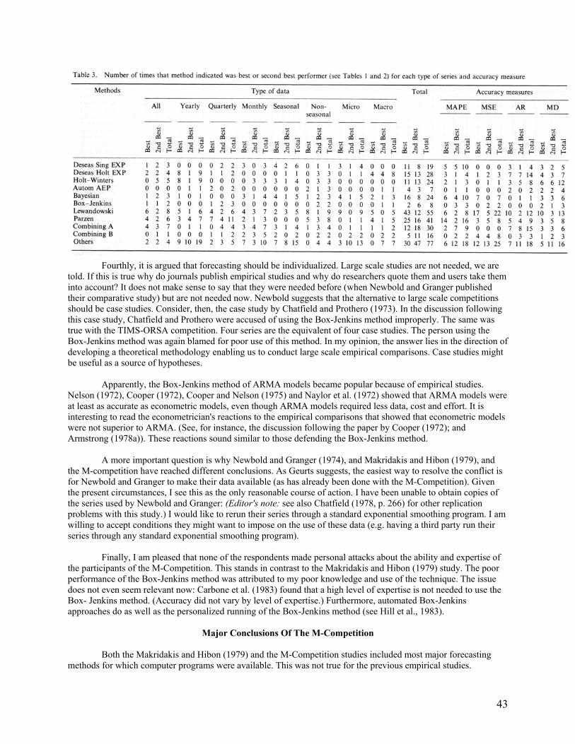
43

Fourthly, it is argued that forecasting should be individualized. Large scale studies are not needed, we are told. If this is true why do journals publish empirical studies and why do researchers quote them and users take them into account? It does not make sense to say that they were needed before (when Newbold and Granger published their comparative study) but are not needed now. Newbold suggests that the alternative to large scale competitions should be case studies. Consider, then, the case study by Chatfield and Prothero (1973). In the discussion following this case study, Chatfield and Prothero were accused of using the Box-Jenkins method improperly. The same was true with the TIMS-ORSA competition. Four series are the equivalent of four case studies. The person using the Box-Jenkins method was again blamed for poor use of this method. In my opinion, the answer lies in the direction of developing a theoretical methodology enabling us to conduct large scale empirical comparisons. Case studies might be useful as a source of hypotheses.

Apparently, the Box-Jenkins method of ARMA models became popular because of empirical studies.

Nelson (1972), Cooper (1972), Cooper and Nelson (1975) and Naylor et al. (1972) showed that ARMA models were at least as accurate as econometric models, even though ARMA models required less data, cost and effort. It is interesting to read the econometrician's reactions to the empirical comparisons that showed that econometric models were not superior to ARMA. (See, for instance, the discussion following the paper by Cooper (1972); and Armstrong (1978a)). These reactions sound similar to those defending the Box-Jenkins method.

A more important question is why Newbold and Granger (1974), and Makridakis and Hibon (1979), and

the M-competition have reached different conclusions. As Geurts suggests, the easiest way to resolve the conflict is for Newbold and Granger to make their data available (as has already been done with the M-Competition). Given the present circumstances, I see this as the only reasonable course of action. I have been unable to obtain copies of the series used by Newbold and Granger: (Editor's note: see also Chatfield (1978, p. 266) for other replication problems with this study.) I would like to rerun their series through a standard exponential smoothing program. I am willing to accept conditions they might want to impose on the use of these data (e.g. having a third party run their series through any standard exponential smoothing program).

Finally, I am pleased that none of the respondents made personal attacks about the ability and expertise of

the participants of the M-Competition. This stands in contrast to the Makridakis and Hibon (1979) study. The poor performance of the Box-Jenkins method was attributed to my poor knowledge and use of the technique. The issue does not even seem relevant now: Carbone et al. (1983) found that a high level of expertise is not needed to use the Box- Jenkins method. (Accuracy did not vary by level of expertise.) Furthermore, automated Box-Jenkins approaches do as well as the personalized running of the Box-Jenkins method (see Hill et al., 1983).

Major Conclusions Of The M-Competition

Both the Makridakis and Hibon (1979) and the M-Competition studies included most major forecasting methods for which computer programs were available. This was not true for the previous empirical studies.

44

Furthermore, special steps were taken in the M-Competition to provide for objectivity and replicability. The conclusions of these two empirical studies are radically changing forecasting practices. Furthermore, some of these conclusions have been obtained independently by other studies (see Gardner and Dannenbring, 1980; Gardner, 1983; Mahmoud, 1984).

In the remaining part of this paper I present my major conclusions from the M-Competition. At the same

time, I suggest how they might affect the field of forecasting. Before the Makridakis and Hibon (1979) study the prevailing opinion among academic forecasters

(including myself; see page 7 of Makridakis and Wheelwright, 1978) was that the BoxJenkins method was the most accurate forecasting technique available. (For an exception to this view see Armstrong, 1978b, p.159.) The prevailing opinion now is that the best method varies depending upon the situation. This is an important change in attitudes. The M-Competition shows that simpler methods should not be dismissed out of hand.

It is not easy to summarize the evidence from the M-Competition. However, one way to summarize the

results is by identifying the best and the second best methods. This has been done in Tables 1 and 2 for the 111 series sample on which all methods were applied. Table 3 is a summary of Tables 1 and 2.

The M-Competition showed three conditions that affect forecasting accuracy: the time horizon of

forecasting, the type of data used, and the accuracy measure computed. Various methods do better or worse depending upon these three conditions. Looking at Table 1, for example, Parzen's method is always the best in MAPS, for quarterly data, for each and all forecasting horizons. However, it does riot do as well in the MSE measure where Lewandowski is best three times and Holt is best the fourth. Similarly, single exponential smoothing is the best method for one-period ahead forecasts but, as it should be expected, does not do well for longer horizons.

Table 1 shows the best (denoted by B) method among those listed. Table 2 shows the second best (denoted

by b). This is only one of the many possible ways to summarize the results. A disadvantage inherent in the use of Tables 1 and 2 is that equal weight is given to all entries. Being the best in the “average of all forecasts” is more important than that of “one period ahead forecast” (which is one of the entries being averaged in the “average of all forecasts”). Another disadvantage is the double counting that occurs in Tables 1 and 2, in that a single series can be monthly, seasonal and micro.

Table 3 is a summary of Tables 1 and 2. It clearly shows that the three best methods for the sample of 111

series are Lewandowski's FORSYS, Parzen's ARARMA, and Holt's exponential smoothing. Two other methods that do well are Bayesian forecasting and single exponential smoothing. Finally, Combining A also does well, trailing only Lewandowski and Parzen.

Tables 1, 2 and 3 provide overall summaries of the results. Looking at these three tables as well as

individual tables published in the M-Competition, I suggest the following hypotheses:

1. Lewandowski's method is the best for longer forecasting horizons (six periods ahead or longer). FORSYS does not extrapolate past trends linearly, but rather it dampens them in a manner determined by the long- term trend of the series (see Lewandowski, 1979). Lewandowski also does well on the MSE criterion, outperforming all other methods. In addition, Lewandowski is the best with monthly and micro data.

2. Deseasonalizing the data through a simple classical decomposition procedure works well. The

deseasonalizing of the data, followed by the use of Holt's linear exponential smoothing, produced more accurate results than Winter's exponential smoothing (which is equivalent to Holt's, except that it takes seasonality directly into account).

3. Deseasonalized single exponential smoothing is the best method overall, when a one-period ahead forecast

is needed. Holt's is the next most appropriate method.

4. For four forecasting horizons ahead, Parzen's method is the best. This is also true with quarterly data.

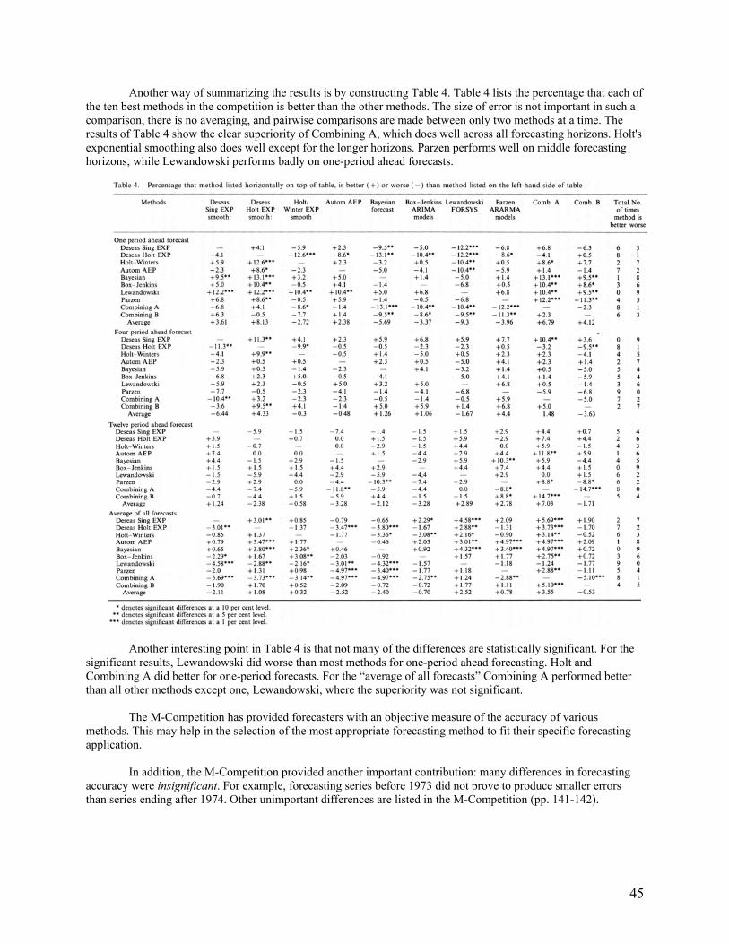
45

Another way of summarizing the results is by constructing Table 4. Table 4 lists the percentage that each of the ten best methods in the competition is better than the other methods. The size of error is not important in such a comparison, there is no averaging, and pairwise comparisons are made between only two methods at a time. The results of Table 4 show the clear superiority of Combining A, which does well across all forecasting horizons. Holt's exponential smoothing also does well except for the longer horizons. Parzen performs well on middle forecasting horizons, while Lewandowski performs badly on one-period ahead forecasts.

Another interesting point in Table 4 is that not many of the differences are statistically significant. For the

significant results, Lewandowski did worse than most methods for one-period ahead forecasting. Holt and Combining A did better for one-period forecasts. For the “average of all forecasts” Combining A performed better than all other methods except one, Lewandowski, where the superiority was not significant.

The M-Competition has provided forecasters with an objective measure of the accuracy of various

methods. This may help in the selection of the most appropriate forecasting method to fit their specific forecasting application.

In addition, the M-Competition provided another important contribution: many differences in forecasting

accuracy were insignificant. For example, forecasting series before 1973 did not prove to produce smaller errors than series ending after 1974. Other unimportant differences are listed in the M-Competition (pp. 141-142).

46

Conclusion

Large-scale empirical studies of forecasting methods are not easy to conduct. They require much time and effort. Problems arise because of a lack of a precise methodology. Furthermore, we need to learn more about the various accuracy measures and their implications. On the other hand, the results of empirical studies are useful for both theoretical and practical work. More studies are needed. Research is required to improve the methodology of empirical comparisons to understand why theoretical predictions such as “ARMA models must be more accurate than exponential smoothing methods since the latter is a special case of the former,” do not hold true. Using Newbold's analogy, we must learn why thoroughbred horses behaved like mules in the “horse-race.”

References

The initials following each reference indicate who cited each of the items. Andersen, A. (1983), “An empirical examination of Box-Jenkins forecasting,” Journal of the Royal Statistical

Society A, 145, 472-475. (AA) Armstrong, J. Scott (1978a), “Forecasting with econometric methods: Folklore vs. fact,” Journal of Business, 51,

549-564. (JSA) (SM) Armstrong, J. Scott (1978b), Long-Range Forecasting: From Crystal Ball to Computer. New York: Wiley. (AA)

(ESG) (SM) (PN) Armstrong, J. Scott (1982), “Research on scientific journals: Implications for editors and authors,” Journal of

Forecasting, 1, 83-104. (JSA) (DJ P) Bates, J. M. and Granger, C. W. J. (1969), “Combination of forecasts,” Operational Research Quarterly, 20

451-468. (MDG) Bunn, Derek W. (1979), “The synthesis of predictive models in marketing research,” Journal of Marketing

Research, 16, May, 280-283. (MDG) Box, G. E. P. and Jenkins, G. M. (1970), Time Series Analysis, Forecasting and Control. San Francisco: Holden

Day. (DJP) Carbone, Robert and Armstrong, J. S. (1982), “Evaluation of extrapolative forecasting methods: Results of a survey

of academicians and practitioners,” Journal of Forecasting, 1, 215-217. (ESG) (DJP) (JSA) Carbone, Robert, et al. (1983), “Comparing for different time series methods the value of technical expertise,

individualized analysis, and judgmental adjustment,” Management Science, 29, 559-566. (RC) (SM) Chatfield, C. (1978), “The Holt-Winters forecasting procedure,” Applied Statistics, 27, 264-279. (SM) (JSA) Chatfield, C. and Prothero, D. L. (1973), “Box- Jenkins seasonal forecasting: Problems in a case study,” Journal of

the Royal Statistical Society A, 136, 295-336. (SM) Christ, Carl (1951), Conference on Business Cycles. Cambridge: National Bureau of Economic Research. (RLM) Cleveland, W. P. and Tiao, G. C. (1976), “Decomposition of seasonal time series: A model for the census X-11

program,” Journal of the American Statistical Association, 71, 581-587. (PN) Cole, LaMont C. (1957), “Biological clock in the unicorn,” Science, 125, 874-876. (LL) Cooper, J. P. and Nelson, C. R. (1975), “The ex ante performance of the St. Louis and FRB-MIT-PENN

econometric models and some results on composite predictors,” Journal of Money, Credit and Banking, 7, 1-32. (SM)

47

Cooper, R. L. (1972), “The predictive performance of quarterly econometric models of the United States,” in

Hickman, B. G. (ed.) Econometric Models of Cyclical Behavior. New York: National Bureau of Economic Research. (SM)

Davies, N. and Newbold, P. (1979), “Some power studies of a portmanteau test of time series model specification,”

Biometrika, 66, 153-155. (PN) Davies, N., Triggs, C. M. and Newbold, P. (1977), “Significance levels of the Box-Pierce portmanteau statistic in

finite samples,” Biometrika, 64, 517-522. (PN) Durbin, J. (1979), “Discussion of paper by Makridakis and Hibon,” Journal of the Royal Statistical Society, A,142,

13, 3-134. (PN) Ehrenberg, A. S. C. (1981), “The problem of numeracy,” The American Statistician, 35(2), May, 67-71. (DJP) (SM) Ekern, S. (1981), “Adaptive exponential smoothing revisited,” Journal of the Operational Research Society, 32,

775-782. (ESG) Ekern, S. (1982), “On simulation studies of adaptive forecasts,” Omega, 10, 91-93. (ESG) Fildes, Robert (1979), “Quantitative forecasting-the state of the art: Extrapolative models,” Journal of the

Operational Research Society, 30, 691-710. (RF) Fildes, Robert (1982), “An evaluation of Bayesian forecasting,” Working Paper, 77, Manchester Business School.

(RF) Fildes, Robert (1983), “An evaluation of Bayesian forecasting,” Journal of Forecasting, 2, 137-150. (RF) Friedman, Milton, Comment on a Test of an Econometric Model. Cambridge: National Bureau of Economic

Research, 1951. (RLM) Gardner, Everette S. Jr. (1983), “Automatic monitoring of forecast errors,” Journal of Forecasting, 2, 1-21. (SM) Gardner, Everette, S. Jr. and Dannenbring, D. G. (1980), “Forecasting with exponential smoothing: Some guidelines

for model selection,” Decision Sciences, 11, 370-383. (JSA) (ESG) (SM) Granger, C. W. J. and Newbold, P. (1977), Forecasting Economic Time Series. New York: Academic Press. (AA) Granger, C. W. J. and Newbold, P. (1973), “Some comments on the evaluation of economic forecasts,” Applied

Economics, 5, 35-47. (PN) Gilchrist, W. G. (1979), “Discussion of the paper by Professor Makridakis and Dr. Hibon,” Journal of the Royal

Statistical Society, A, 142, Part 2, 146-147. (MDG) Green, D. M. and Swets, J. A. (1966), Signal Detection Theory and Psychophysics. New York: Robert E. Krieger.

(LLL) Harnad, Stevan (1979), “Creative disagreement,” The Sciences, 19, 18-20. (JSA) Hickman, W. Braddock (1942), The Term Structure of lnterest Rates. Cambridge: National Bureau of Economic

Research. (RLM) Hill, Gareth and Fildes, Robert, “The accuracy of extrapolation methods; an automatic Box-Jenkins package:

SIFT,” Journal of Forecasting, 3, 319-323. (RF) (SM)

48

Jenkins, Gwilym, M., “Some practical aspects of forecasting in organizations,” Journal of Forecasting, 1 (1982), 3-21. (RF) (ESG) (DJ P)

Lewandowski, R. (1979), La Prevision d Court Terme. Paris: Dunod. (SM) Lopes, Lola L. (1982), “Doing the impossible: A note on induction and the experience of randomness,” Journal of

Experimental Psychology: Learning, Memory, and Cognition, 8, 626-636. (LLL) Lopes, Lola L. and Oden, Gregg C. (1981), “Distinguishing between random and nonrandom events,” paper

presented at Eighth Research Conference on Subjective Probability, Utility, and Decision Making, Budapest, Hungary, August. (LLL)

Mahmoud, Essam (1984), “Accuracy in forecasting: A survey,” Journal of Forecasting, 3, 139-159. (SM) Makridakis, Spyros, Andersen, A., Carbone, R., Fildes, R., Hibon, M., Lewandowski, R., Newton, J., Parzen, E. and

Winkler, R. (1982), “The accuracy of extrapolation (time series) methods: Results of a forecasting competition,” Journal of Forecasting, 1, 111-153. (all)

Makridakis, Spyros, Andersen, A., Carbone, R., Fildes, R., Hibon, M., Lewandowski, R., Newton, J., Parzen, E. and

Winkler, R. (1984), The Accuracy of Time Series Methods. New York, John Wiley. (RC) Makridakis, Spyros and Hibon, Michele (1979), “Accuracy of forecasting: An empirical investigation,” Journal of

the Royal Statistical Society, A, with discussion, 142, 97-145. (AA) (RF) (MDG) (PN) (SM) Makridakis, Spyros and Wheelwright, S. (1978), Interactive Forecasting: Univariate and Multivariate Methods.

San Francisco: Holden-Day. (SM) Makridakis, Spyros and Winkler, Robert, L. (1983), “Averages of forecasts: Some empirical results,” Management

Science, 29, 987-996. (RLW) McClain, J. O. (1974), “Dynamics of exponential smoothing with trend and seasonal terms,” Management Science,

20, 1300-1304. (ESG) McClain, J. O. and Thomas, L. J. (1973), “Response-variance tradeoffs in adaptive forecasting,” Operations

Research, 21, 554-568. (ESG) Naylor, Thomas H. et al. (1972), “Box-Jenkins methods: An alternative to econometric forecasting,” International

Statistical Review, 40, 123-137. (SM) Nelson, C. R. (1972), “The prediction performance of the FRB-MIT-PENN model of the U.S. economy,” American

Economic Review, 62, 902-917. (SM) Newbold, Paul and Granger, C. W. J. (1974), “Experience with forecasting univariate time series and the

combination of forecasts,” Journal of the Royal Statistical Society, A,137, 131-165. (AA) (MDG) (PN) (RLW) (SM)

Newton, H. J., “Using periodic autoregression for multiple spectral estimation,” Technometrics, 24 (1982), 109-116.

(E P) Pack, David J. (1982), “Measures of forecast accuracy,” presented to the ORSA/TIMS 1982 Joint National Meeting,

San Diego, California, October 25-27. (SM) (DJP) Parzen, Emanuel (1979), “Nonparametric statistical data modeling,” Journal of the American Statistical

Association, with discussion, 74, 105-131. (EP)

49

Parzen, Emanuel (1981), “Time series model identification and prediction variance horizon,” Findley, D. (ed.) Applied Time Series Analysis, 11, New York: Academic Press, pp. 415-447. (EP)

Reinmuth, James E. and Geurts, Michael D. (1979), “A multideterministic approach to forecasting,” TIMS Studies

in the Management Sciences, 12, 203-211. (MDG) Slutzky, Eugene (1937), “The summation of random causes as the source of cyclic processes,” Econometrica, 5,

105-146. (LLL) Tversky, A. and Kahneman, D. (1973), “Availability: a heuristic for judging frequency and probability,” Cognitive

Psychology, 5, 207-232. (LLL) Wagenaar, Willem A. (1972), “Generation of random sequences by human subjects: A critical survey of literature,”

Psychological Bulletin, 77, 65-72. (LLL) Wason, P. C. (1960), “On the failure to eliminate hypotheses in a conceptual task,” Quarterly Journal of

Experimental Psychology, 12, 129-140. (SM). Winkler, Robert L. and Makridakis, Spyros (1983), “The combination of forecasts,” Journal of the Royal Statistical

Society, A, 146, 150-157. (RLW)

Commentary on the Makridakis Time Series Competition (M

Documents